Embed Size (px)
Citation preview
Progression of spontaneous in-plane shear faultsfrom sub-Rayleigh to compressional waverupture speedsChao Liu1, Andrea Bizzarri2, and Shamita Das1
1Department of Earth Sciences, University of Oxford, Oxford, UK, 2Istituto Nazionale di Geofisica e Vulcanologia, Bologna, Italy
Abstract We investigate numerically the passage of spontaneous, dynamic in-plane shear ruptures frominitiation to their final rupture speed, using very fine grids. By carrying out more than 120 simulations, weidentify two different mechanisms controlling supershear transition. For relatively weaker faults, the rupturespeed always passes smoothly and continuously through the range of speeds between the Rayleigh and shearwave speeds (the formerly considered forbidden zone of rupture speeds). This, however, occurs in a very shorttime, before the ruptures reach the compressional wave speed. The very short time spent in this range ofspeeds may explain why a jump over these speeds was seen in some earlier numerical and experimentalstudies and confirms that this speed range is an unstable range, as predicted analytically for steady state,singular cracks. On the other hand, for relatively stronger faults, we find that a daughter rupture is initiated bythe main (mother) rupture, ahead of it. The mother rupture continues to propagate at sub-Rayleigh speed andeventually merges with the daughter rupture, whose speed jumps over the Rayleigh to shear wave speedrange. We find that this daughter rupture is essentially a “pseudorupture,” in that the two sides of the fault arealready separated, but the rupture has negligible slip and slip velocity. After the mother rupture merges withit, the slip, the slip velocity, and the rupture speed become dominated by those of the mother rupture. Theresults are independent of grid sizes and of methods used to nucleate the initial rupture.
1. Introduction
It is now known that in-plane shear faults (primarily strike-slip earthquakes) can not only exceed the shear wavespeed of the medium but can even reach the compressional wave speed (this is commonly referred to assupershear earthquakes in the geophysical literature or analogously as intersonic ruptures in the framework offracture mechanics). This result is based on theoretical and numerical studies [Burridge, 1973; Andrews, 1976;Das and Aki, 1977; Burridge et al., 1979; Freund, 1979; Geubelle and Kubair, 2001; Bizzarri et al., 2001; Festa andVilotte, 2006; Dunham, 2007; Liu and Lapusta, 2008; Lu et al., 2009], laboratory experiments [Rosakis et al., 1999;Rosakis, 2002; Xia et al., 2004, 2005; Lu et al., 2007; Rosakis et al., 2007; Passelègue et al., 2013] and indirect evidencebased upon seismic data analysis [Archuleta, 1984; Olsen et al., 1997; Bouchon et al., 2001; Bouchon and Vallée,2003; Dunham and Archuleta, 2004; Ellsworth et al., 2004; Robinson et al., 2006; Bhat et al., 2007; Vallée et al., 2008].
On the other hand, analytical calculations made on steady state singular cracks [Broberg, 1994, 1995, 1999]and numerical studies on spontaneous nonsingular cracks [Andrews, 1976] show that speeds betweenthe Rayleigh and shear wave speeds are not possible. In such a case there is negative energy flux into thefault edge from the surrounding medium. The fault would not absorb strain energy but generate it (seeBroberg [1999] for details). In a pioneering numerical study, Andrews [1976] showed that the forbiddenzone does exist, even for nonsingular, 2-D, in-plane faults which start from rest and spontaneouslyaccelerate to some terminal velocity. The existence of this “forbidden zone” in rupture speed has beensupported by many studies, both analytical [Burridge et al., 1979] and numerical [Liu and Lapusta, 2008;Lu et al., 2009]. Geubelle and Kubair [2001] studied this problem numerically using a spectral boundaryintegral equation method. Though they find similar results as above, they do not find the forbidden zone.Instead, they schematically demonstrate that for most of their cases, the rupture front passes rapidly andsmoothly through the forbidden zone, although the initiation procedure of the rupture is not describedin detail, and the (numerical) resolution of the forbidden zone is not shown. They also do not clarify whythis happens for some configurations and their insights are retrieved from the location (and shape) of therupture front (and not from a formal computation of the rupture speed).
LIU ET AL. ©2014. American Geophysical Union. All Rights Reserved. 1
PUBLICATIONSJournal of Geophysical Research: Solid Earth
RESEARCH ARTICLE10.1002/2014JB011187
Key Points:• Supershear rupture transitionsstudied numerically
• For weaker faults, rupture speedsincrease continuously to supershear
• For stronger faults, the rupture jumpsahead with negligible slip and slip rate
Supporting Information:• Readme• Animation S1• Animation S2• Figure S1• Figure S2
Correspondence to:C. Liu,[email protected]
Citation:Liu, C., A. Bizzarri, and S. Das (2014),Progression of spontaneous in-planeshear faults from sub-Rayleigh tocompressional wave rupture speeds,J. Geophys. Res. Solid Earth, 119,doi:10.1002/2014JB011187.
Received 11 APR 2014Accepted 19 OCT 2014Accepted article online 27 OCT 2014
Recently, Bizzarri and Das [2012] showed that therupture front actually does pass through the [vR, vS]range of speeds, and very fast. Unprecedented finegrids are used in their numerical experiments for atruly 3-D shear ruptures (in which the in-plane(mode II) and the antiplane (mode III) are mixedtogether) propagating on a planar fault and obeyingthe linear slip-weakening governing model.
Motivated by these results, here we examine indetail, using very fine grids, the 2-D pure modeII case to see the passage of the rupture frontfrom sub-Rayleigh to the compressional wavespeeds. The 2-D problem is of interest becausefor very long strike-slip faults in the Earth’s crustthe rupture becomes primarily pure mode II atlarge distances from the hypocenter (that is,when the fault length is much larger than itswidth). In addition to the inherent theoreticalissues, the interest in supershear ruptures ismotivated by very practical implications.Compared to subsonic events, the supershearruptures produce stronger shaking farther from
the fault and are richer in high frequencies [Aagaard and Heaton, 2004; Bhat et al., 2007; Bizzarri andSpudich, 2008; Bizzarri et al., 2010].
To investigate the entire range of possible rupture speeds from rupture initiation to the compressional wavespeed, numerical experiments are carried out to mainly cover the parameter space where supershear rupturepropagation could occur. A few cases where the rupture speed remains below the Rayleigh wave speed are alsostudied. The small grid sizes used in this study provide a very good resolution of the rupture speed, allowing us toexamine the details of the rupture progress from sub-Rayleigh to compressional wave speeds. It is worthwhileto emphasize here that most of the previous studies, instead of showing the actual values of the rupture speedsobtained through numerical calculations, merely plot schematic figures of the rupture speed evolution. Liu andLapusta [2008] and Lu et al. [2009] show the rupture speeds, averaged over a broad moving window.
The present paper is organized as follows. In section 2 we present the geometry of the problem. Thenumerical results are shown in section 3, where we present the two different mechanisms which control thesupershear transition. In section 4 we discuss the distance from the nucleation patch at which the supersheartransition occurs, and we present a phase diagram to compare against previous results of Andrews [1976]and summarize the major conclusions of this study. Technical details on the estimate of the rupture speed,the effect of nucleation methods, and different spatial grid sizes are thoroughly discussed in the threeappendices (Appendix A–Appendix C, respectively).
2. Fault Geometry and Rupture Nucleation
In the present study we consider a 2-D, pure in-plane shear (mode II) rupture problem, as shown in Figure 1. Therupture propagates along x1; the solutions (e.g., the displacement discontinuity) do not depend on x2 and haveonly one component (e.g., u1(x1, t); for the sake of simplicity, in the remainder of the paper we will omit thesubscripts). The elastodynamic problem, in which body forces are neglected, is numerically solved by using thefinite difference code described in Bizzarri et al. [2001], originally developed by Andrews [1973], which uses amesh of triangles and the leap-frog scheme. The code has beenmademore efficient by us using parallelizationthrough the OpenMP paradigm. We assume that the fault obeys the linear slip-weakening friction law [Ida,
1972], which is expressed by the following relation: τ uð Þ ¼ σeffn μu � μu � μfð Þmin u; d0ð Þ=d0½ �, where τ is the
magnitude of the shear stress on the fault, σeffn is the effective normal stress (assumed to be constant throughtime), μu is the static friction coefficient, μf is the dynamic friction coefficient, u is the fault slip, and d0 is thecharacteristic slip-weakening distance. The parameters used in this study are listed in Table 1.
Figure 1. Geometry of the fault. The dotted line indicatesthe fault trace. The rupture begins at the hypocenter H andpropagates bilaterally, as shown by the arrows. Lf is the halflength of the fault. Due to the symmetry of the problem, onlyone half of the fault is considered (as indicated).
Journal of Geophysical Research: Solid Earth 10.1002/2014JB011187
LIU ET AL. ©2014. American Geophysical Union. All Rights Reserved. 2
Choices of the ratio C= vPΔt/Δx andpossible rupture speed values thatcan be resolved numerically arediscussed in detail in the Appendix A(Δt and Δx are the temporal and thespatial grid sizes, respectively). Forthe second-order accurate, explicit,2-D finite difference schemeemployed here, the Courant-Friedrichs-Lewy condition is C ≤ 0.71[Mitchell, 1976] and ensures thestability and the convergence of thenumerical solution. We can choose Cor Δt as small as we like, as long asrounding and magnification errorsremain negligible.
In order to initiate a rupture governed by the linear slip-weakening friction law, we use an (artificial)nucleation procedure to trigger the dynamic propagation. Once the nucleation stage is completed, therupture propagates spontaneously. The rupture speed vr is not prescribed (as for nonspontaneous problems)but is a part of the solution itself. In the present paper we adopt two rupture nucleation strategies withdifferent initial parameters. In the first strategy, called the time-weakening initiation, the rupture is initiallynonspontaneous and it propagates at a constant, prescribed rupture speed vr= vinit [Andrews, 1985; Bizzarri,2010]. Values of vinit equal to 1.2 km/s and 5 km/s are tested. In the second strategy, called the asperityinitiation, a small perturbation in initial shear stress is used to trigger the dynamic rupture [Bizzarri, 2010]. Thesize of the asperity should be small enough to avoid interference with the subsequent spontaneous rupturepropagation. The details of the methods and their effect, if any, are fully discussed and quantitativelycompared in Appendix B.
3. Numerical Results for 2-D Spontaneous Rupture Propagation
One hundred and twenty six numerical experiments are carried out in this study. They are sorted into sixConfigurations, named as A to F. For each configuration we investigate the relation existing between therupture speed and the strength parameter S, originally defined by Hamano [1974] as S= (τu� τ0)/(τ0� τf ),where τu ¼ μuσ
effn is the upper yield stress, τ0 is the initial shear stress, and τf ¼ μfσ
effn is the residual shear
stress. The numerator represents the so-called strength excess (i.e., the amount of stress needed to reachthe failure point) and the denominator represents the dynamic stress drop. Thus, doubling the value of thisstress drop simply reduces S by a factor of 2. In addition, a fault with the same strength would have a differentvalue of S if its initial stress is changed. From here on, we shall refer to weaker/more stressed or a relativelyweaker fault as a “weak fault” and vice versa for a “strong fault.”
We consider 24 values of S in the range between 0.38 and 1.2, and 6 values larger than 1.2. To obtain differentvalues of S, we change the upper yield stress τu, and we keep the other parameters unchanged. Contrary to the3-D case, where the absolute values of the stresses affect the behavior of the propagating rupture (they indeed
Table 1. Parameters Adopted for the 126 Cases in This Studya
Parameter Value
Lamé’s constants, λ = G 35.9 GPaS wave speed, vS 3.464 km/sRayleigh speed, vR 3.184 km/sEshelby speed, vE ¼
ffiffiffi2
pvs 4.899 km/s
P wave speed, vP 6 km/sEffective normal stress, σeffn 120MPaInitial shear stress (prestress), τ0 73.8MPaDynamic friction coefficient, μf 0.46Dynamic friction level, τf 55.2MPaDynamic stress drop, τ0� τf 18.6MPaCharacteristic slip-weakening distance, d0 0.4mC = vPΔt/Δx
b 0.0514
aWe consider homogeneous properties and a constant effective normalstress. Except for C, all parameters are the same as in Bizzarri and Das [2012].
bΔt is the time step and Δx is the spatial grid length.
Table 2. Parameters Used in Configurations A to Ea
Configuration Δx (m) Δt (s) Number Of Cases Nucleation Method
A 40 3.42 × 10�4 24 TWb: vinit = 0.5 km/sB 20 1.71 × 10�4 24 ’’C 10 8.57 × 10�5 24 ’’D 40 3.42 × 10�4 24 TWb: vinit = 1.2 km/sE 40 3.42 × 10�4 24 Asperity
aThe fault half-length Lf = 40 km is used for all the configurations.bTW: Time-weakening with starting speed vinit.
Journal of Geophysical Research: Solid Earth 10.1002/2014JB011187
LIU ET AL. ©2014. American Geophysical Union. All Rights Reserved. 3
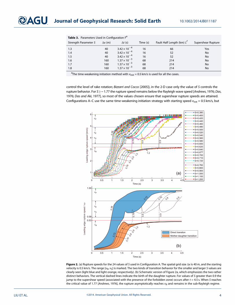
control the level of rake rotation; Bizzarri and Cocco [2005]), in the 2-D case only the value of S controls therupture behavior. For S≥~1.77 the rupture speed remains below the Rayleigh wave speed [Andrews, 1976; Das,1976; Das and Aki, 1977], so most of the values chosen ensure that supershear rupture speeds are attained.Configurations A–C use the same time-weakening initiation strategy with starting speed vinit = 0.5 km/s, but
Table 3. Parameters Used in Configuration Fa
Strength Parameter S Δx (m) Δt (s) Time (s) Fault Half Length (km) Lf Supershear Rupture
1.3 40 3.42 × 10�4 16 66 Yes1.4 40 3.42 × 10�4 16 52 No1.5 40 3.42 × 10�4 16 52 No1.6 160 1.37 × 10�3 68 214 No1.7 160 1.37 × 10�3 68 214 No1.8 160 1.37 × 10�3 68 214 No
aThe time-weakening initiation method with vinit = 0.5 km/s is used for all the cases.
Figure 2. (a) Rupture speeds for the 24 values of S used in Configuration A. The spatial grid size Δx is 40m, and the startingvelocity is 0.5 km/s. The range [vR, vS] is marked. The two kinds of transition behavior for the smaller and larger S values areclearly seen (light blue and light orange, respectively). (b) Schematic version of Figure 2a, which emphasizes the two ratherdistinct behaviors. The vertical dashed lines indicate the birth of the daughter rupture. For values of S greater than 0.9 thejump to the supershear speed (associated with the presence of the forbidden zone) occurs after t = 4.5 s. When S reachesthe critical value of 1.77 [Andrews, 1976], the rupture asymptotically reaches vR and remains in the sub-Rayleigh regime.
Journal of Geophysical Research: Solid Earth 10.1002/2014JB011187
LIU ET AL. ©2014. American Geophysical Union. All Rights Reserved. 4
different spatial grid sizes, Δx = 40m,20m, and 10m. Configurations D and Euse the same spatial grid length Δx =40m as Configuration A, but differentnucleation methods. Configuration Duses the time-weakening initiationstrategy with starting speed vinit =1.2 km/s, and Configuration E uses theasperity initiation strategy. The relevantparameters for these six Configurationsare listed in Table 2. For comparison, wealso study six cases (S> 1.2) where it isdifficult or impossible for the rupturespeed to exceed the Rayleigh wavespeed. These cases are grouped togetherin Configuration F. For the cases withS> 1.6, we used larger spatial grids(Δx = 160m) as it takes longer for therupture to propagate (the parameters aregiven in Table 3).
3.1. Supershear Rupture for WeakerFaults (~0.38 ≤ S ≤~0.72): The DirectTransition Mechanism
For this range of S the fault is relativelyweak and the supershear rupture occurssoon after nucleation. We chooseS ≥ 0.38 as lower boundary of thisinterval simply to give enough time forthe rupture to become spontaneous andto avoid any possible artificial effect ofthe nucleation methods. The rupturespeed versus time for this range of S isshown in Figure 2a, with a schematicsummary version shown in Figure 2b.This figure pertains to Δx = 40m, but theresults for Δx = 20m and Δx = 10m arevery similar (see the results shown inAppendix C), which indicates that ourconclusions are independent of thespatiotemporal grid lengths.
The rupture speed curves for this range of S in Figure 2a form a completely separate group (light blue inFigure 2b) from faults with larger values of S (light orange in Figure 2b). We see that the rupture starts fromrest, accelerates and passes smoothly through the range [vR, vS], and then approaches the compressionalwave speed vP. This direct transition mode has been studied by [Geubelle and Kubair, 2001; Festa and Vilotte,2006; Dunham, 2007; Liu and Lapusta, 2008; Lu et al., 2009]. The prominent result to be highlighted hereis that the forbidden zone has been shown to or implied to exist for this range of S in some of these studies[Liu and Lapusta, 2008; Lu et al., 2009]. The present study—which adopts very fine grids with a properrupture speed resolution in the [vR, vS] (see Appendix A)—quantitatively demonstrates that the rupturespeed evolves continuously and passes through this range of rupture velocities during direct transition. Forsuch faults the rupture speed continuously increases from sub-Rayleigh to supershear without any jump.We also see (Figure S1 in the supporting information) that the time spent in the [vR, vS] regime isindependent of the grid size.
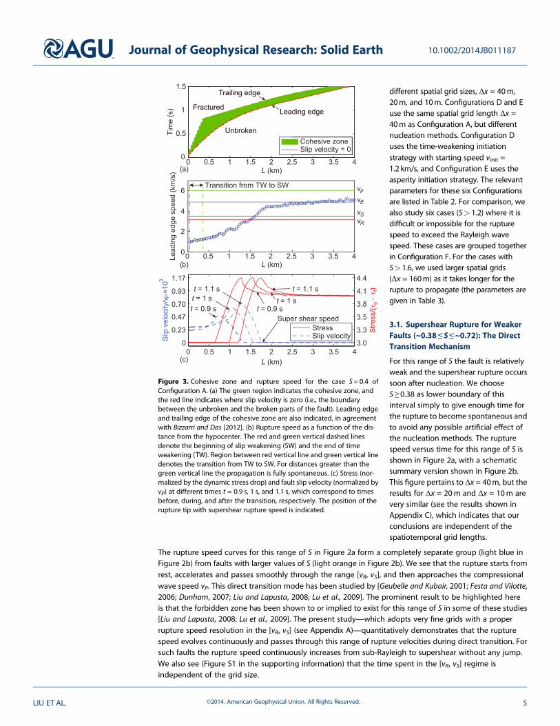
Figure 3. Cohesive zone and rupture speed for the case S = 0.4 ofConfiguration A. (a) The green region indicates the cohesive zone, andthe red line indicates where slip velocity is zero (i.e., the boundarybetween the unbroken and the broken parts of the fault). Leading edgeand trailing edge of the cohesive zone are also indicated, in agreementwith Bizzarri and Das [2012]. (b) Rupture speed as a function of the dis-tance from the hypocenter. The red and green vertical dashed linesdenote the beginning of slip weakening (SW) and the end of timeweakening (TW). Region between red vertical line and green vertical linedenotes the transition from TW to SW. For distances greater than thegreen vertical line the propagation is fully spontaneous. (c) Stress (nor-malized by the dynamic stress drop) and fault slip velocity (normalized byvP) at different times t = 0.9 s, 1 s, and 1.1 s, which correspond to timesbefore, during, and after the transition, respectively. The position of therupture tip with supershear rupture speed is indicated.
Journal of Geophysical Research: Solid Earth 10.1002/2014JB011187
LIU ET AL. ©2014. American Geophysical Union. All Rights Reserved. 5
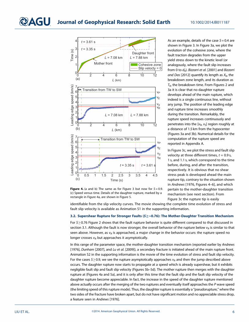
As an example, details of the case S=0.4 areshown in Figure 3. In Figure 3a, we plot theevolution of the cohesive zone, where thefault traction degrades from the upperyield stress down to the kinetic level (oranalogously, where the fault slip increasesfrom 0 to d0). Bizzarri et al. [2001] and Bizzarriand Das [2012] quantify its length as Xb, thebreakdown zone length, and its duration asTb, the breakdown time. From Figures 2 and3a it is clear that no daughter rupturedevelops ahead of the main rupture, whichindeed is a single continuous line, withoutany jump. The position of the leading edgeand rupture time increases smoothlyduring the transition. Remarkably, therupture speed increases continuously andpenetrates into the [vR, vS] region roughly ata distance of 1.5 km from the hypocenter(Figures 3a and 3b). Numerical details for thecomputation of the rupture speed arereported in Appendix A.
In Figure 3c, we plot the stress and fault slipvelocity at three different times, t = 0.9 s,1 s, and 1.1 s, which correspond to the timebefore, during, and after the transition,respectively. It is obvious that no shearstress peak is developed ahead the mainrupture tip, contrary to the situation shownin Andrews [1976, Figures 4–6], and whichpertain to the mother-daughter transitionmechanism (see next section). FromFigure 3c the rupture tip is easily
identifiable from the slip velocity curves. The movie showing the complete time evolution of stress andfault slip velocity is available as Animation S1 in the supporting information.
3.2. Supershear Rupture for Stronger Faults (S ≥~0.76): The Mother-Daughter Transition Mechanism
For S ≥ 0.76 Figure 2 shows that the fault rupture behavior is quite different compared to that discussed insection 3.1. Although the fault is now stronger, the overall behavior of the rupture below vR is similar to thatseen above. However, as vR is approached, a major change in the behavior occurs: the rupture speed nolonger crosses vR but approaches it asymptotically.
In this range of the parameter space, the mother-daughter transition mechanism (reported earlier by Andrews[1976], Dunham [2007], and Lu et al. [2009]), a secondary fracture is initiated ahead of the main rupture front.Animation S2 in the supporting information is the movie of the time evolution of stress and fault slip velocity.For the cases S≥ 0.9, we see the rupture asymptotically approaches vR and then the jump described aboveoccurs. The daughter rupture now starts to propagate at a speed which is already supershear, but it exhibitsnegligible fault slip and fault slip velocity (Figures 5b–5d). The mother rupture then merges with the daughterrupture at (Figures 4a and 5a), and it is only after this time that the fault slip and the fault slip velocity of thedaughter rupture become appreciable. In fact, the increase in the speed of the daughter rupture mentionedabove actually occurs after the merging of the two ruptures and eventually itself approaches the Pwave speed(the limiting speed of this rupturemode). Thus, the daughter rupture is essentially a “pseudorupture,”where thetwo sides of the fracture have broken apart, but do not have significant motion and no appreciable stress drop,a feature seen in Andrews [1976].
Figure 4. (a and b) The same as for Figure 3 but now for S = 0.9.(c) Speed versus time. Details of the daughter rupture, marked by arectangle in Figure 4a, are shown in Figure 5.
Journal of Geophysical Research: Solid Earth 10.1002/2014JB011187
LIU ET AL. ©2014. American Geophysical Union. All Rights Reserved. 6
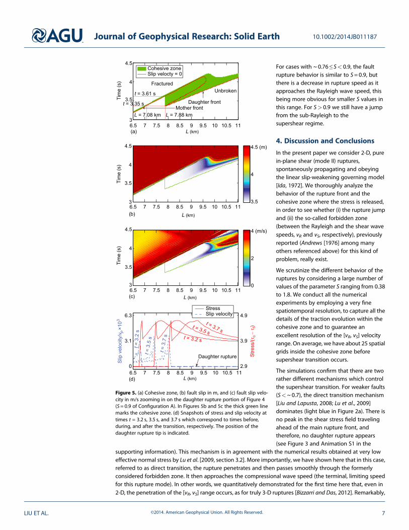
For cases with ~ 0.76 ≤ S< 0.9, the faultrupture behavior is similar to S=0.9, butthere is a decrease in rupture speed as itapproaches the Rayleigh wave speed, thisbeing more obvious for smaller S values inthis range. For S> 0.9 we still have a jumpfrom the sub-Rayleigh to thesupershear regime.
4. Discussion and Conclusions
In the present paper we consider 2-D, purein-plane shear (mode II) ruptures,spontaneously propagating and obeyingthe linear slip-weakening governing model[Ida, 1972]. We thoroughly analyze thebehavior of the rupture front and thecohesive zone where the stress is released,in order to see whether (i) the rupture jumpand (ii) the so-called forbidden zone(between the Rayleigh and the shear wavespeeds, vR and vS, respectively), previouslyreported (Andrews [1976] among manyothers referenced above) for this kind ofproblem, really exist.
We scrutinize the different behavior of theruptures by considering a large number ofvalues of the parameter S ranging from 0.38to 1.8. We conduct all the numericalexperiments by employing a very finespatiotemporal resolution, to capture all thedetails of the traction evolution within thecohesive zone and to guarantee anexcellent resolution of the [vR, vS] velocityrange. On average, we have about 25 spatialgrids inside the cohesive zone beforesupershear transition occurs.
The simulations confirm that there are tworather different mechanisms which controlthe supershear transition. For weaker faults(S<~ 0.7), the direct transition mechanism[Liu and Lapusta, 2008; Lu et al., 2009]dominates (light blue in Figure 2a). There isno peak in the shear stress field travelingahead of the main rupture front, andtherefore, no daughter rupture appears(see Figure 3 and Animation S1 in the
supporting information). This mechanism is in agreement with the numerical results obtained at very loweffective normal stress by Lu et al. [2009, section 3.2]. More importantly, we have shown here that in this case,referred to as direct transition, the rupture penetrates and then passes smoothly through the formerlyconsidered forbidden zone. It then approaches the compressional wave speed (the terminal, limiting speedfor this rupture mode). In other words, we quantitatively demonstrated for the first time here that, even in2-D, the penetration of the [vR, vS] range occurs, as for truly 3-D ruptures [Bizzarri and Das, 2012]. Remarkably,
Figure 5. (a) Cohesive zone, (b) fault slip in m, and (c) fault slip velo-city in m/s zooming in on the daughter rupture portion of Figure 4(S = 0.9 of Configuration A). In Figures 5b and 5c the thick green linemarks the cohesive zone. (d) Snapshots of stress and slip velocity attimes t = 3.2 s, 3.5 s, and 3.7 s which correspond to times before,during, and after the transition, respectively. The position of thedaughter rupture tip is indicated.
Journal of Geophysical Research: Solid Earth 10.1002/2014JB011187
LIU ET AL. ©2014. American Geophysical Union. All Rights Reserved. 7
the forbidden zone can disappear, and it is not auniversal feature of mode II, nonsingular ruptures.The results are accurate and robust; thephenomenon we observe is not an artifact of thenumerical method, the numerical resolution, or themethod employed to nucleate the rupture.
For stronger faults (S>~0.7), the mother-daughter mechanism (also referred to as theBurridge-Andrews mechanism) [Andrews, 1976;Freund, 1979; Abraham and Gao, 2000; Rosakis,2002; Dunham, 2007] dominates in thismechanism. The forbidden zone does exist asthe transition to the intersonic regime involves arupture speed jump.
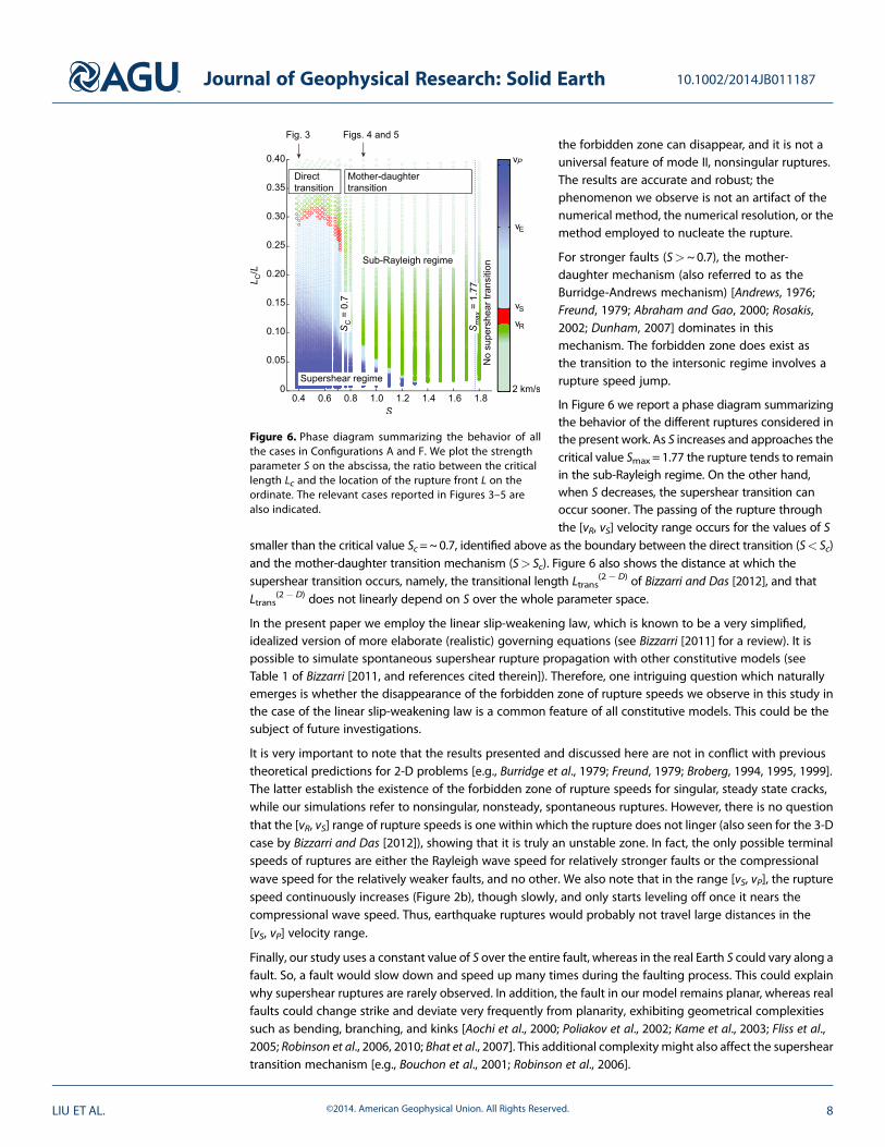
In Figure 6 we report a phase diagram summarizingthe behavior of the different ruptures considered inthe present work. As S increases and approaches thecritical value Smax = 1.77 the rupture tends to remainin the sub-Rayleigh regime. On the other hand,when S decreases, the supershear transition canoccur sooner. The passing of the rupture throughthe [vR, vS] velocity range occurs for the values of S
smaller than the critical value Sc=~0.7, identified above as the boundary between the direct transition (S< Sc)and the mother-daughter transition mechanism (S> Sc). Figure 6 also shows the distance at which thesupershear transition occurs, namely, the transitional length Ltrans
(2� D) of Bizzarri and Das [2012], and thatLtrans
(2� D) does not linearly depend on S over the whole parameter space.
In the present paper we employ the linear slip-weakening law, which is known to be a very simplified,idealized version of more elaborate (realistic) governing equations (see Bizzarri [2011] for a review). It ispossible to simulate spontaneous supershear rupture propagation with other constitutive models (seeTable 1 of Bizzarri [2011, and references cited therein]). Therefore, one intriguing question which naturallyemerges is whether the disappearance of the forbidden zone of rupture speeds we observe in this study inthe case of the linear slip-weakening law is a common feature of all constitutive models. This could be thesubject of future investigations.
It is very important to note that the results presented and discussed here are not in conflict with previoustheoretical predictions for 2-D problems [e.g., Burridge et al., 1979; Freund, 1979; Broberg, 1994, 1995, 1999].The latter establish the existence of the forbidden zone of rupture speeds for singular, steady state cracks,while our simulations refer to nonsingular, nonsteady, spontaneous ruptures. However, there is no questionthat the [vR, vS] range of rupture speeds is one within which the rupture does not linger (also seen for the 3-Dcase by Bizzarri and Das [2012]), showing that it is truly an unstable zone. In fact, the only possible terminalspeeds of ruptures are either the Rayleigh wave speed for relatively stronger faults or the compressionalwave speed for the relatively weaker faults, and no other. We also note that in the range [vS, vP], the rupturespeed continuously increases (Figure 2b), though slowly, and only starts leveling off once it nears thecompressional wave speed. Thus, earthquake ruptures would probably not travel large distances in the[vS, vP] velocity range.
Finally, our study uses a constant value of S over the entire fault, whereas in the real Earth S could vary along afault. So, a fault would slow down and speed up many times during the faulting process. This could explainwhy supershear ruptures are rarely observed. In addition, the fault in our model remains planar, whereas realfaults could change strike and deviate very frequently from planarity, exhibiting geometrical complexitiessuch as bending, branching, and kinks [Aochi et al., 2000; Poliakov et al., 2002; Kame et al., 2003; Fliss et al.,2005; Robinson et al., 2006, 2010; Bhat et al., 2007]. This additional complexity might also affect the supersheartransition mechanism [e.g., Bouchon et al., 2001; Robinson et al., 2006].
Figure 6. Phase diagram summarizing the behavior of allthe cases in Configurations A and F. We plot the strengthparameter S on the abscissa, the ratio between the criticallength Lc and the location of the rupture front L on theordinate. The relevant cases reported in Figures 3–5 arealso indicated.
Journal of Geophysical Research: Solid Earth 10.1002/2014JB011187
LIU ET AL. ©2014. American Geophysical Union. All Rights Reserved. 8
Appendix A: Estimate of theRupture Speed in 2-D NumericalExperiments andIts Limitations
A1. Estimation of the Rupture Speed in 2-D
Rupture speed is an indirect part of thesolution of the spontaneous rupturepropagation problem which has to beretrieved from the rupture times. Such acomputation, although conceptuallystraightforward it is not numerically simple.In this section we test different methods inorder to explore whether the results dependon the assumed numerical algorithm.
By adopting the two-point forwarddifference method, the rupture speed vr(i) ata generic fault node i (having absolutecoordinate xi= iΔx) is
vr ið Þ ¼ i þ 1ð ÞΔx � iΔxtr i þ 1ð Þ � tr ið Þ ¼
Δxtr i þ 1ð Þ � tr ið Þ (A1)
where Δx is the spatial grid length, tr(i) represents the rupture time at node i. According to previous study[Bizzarri and Das, 2012, and references cited therein], the rupture time at node i is defined as the first time atwhich the fault slip velocity in that location exceeds the threshold value vl = 0.01m/s. (Readers can refer tosection 3.1 of Bizzarri [2013] for a discussion.)
Similarly, in the two-point central difference method, the rupture speed vr(i) at node iΔx is
vr ið Þ ¼ i þ 1ð ÞΔx � i � 1ð ÞΔxtr i þ 1ð Þ � tr ið Þ ¼ 2Δx
tr i þ 1ð Þ � tr i � 1ð Þ (A2)
In the five-point stencil difference method, the rupture speed vr(i) at node iΔx is
vr ¼ i � 2ð ÞΔx � 8 i � 1ð ÞΔx þ 8 i þ 1ð ÞΔx � i þ 2ð ÞΔxtr i � 2ð Þ � 8tr i � 1ð Þ þ 8tr i þ 1ð Þ � tr i þ 2ð Þ
¼ 12Δxtr i � 2ð Þ � 8tr i � 1ð Þ þ 8tr i þ 1ð Þ � tr i þ 2ð Þ
(A3)
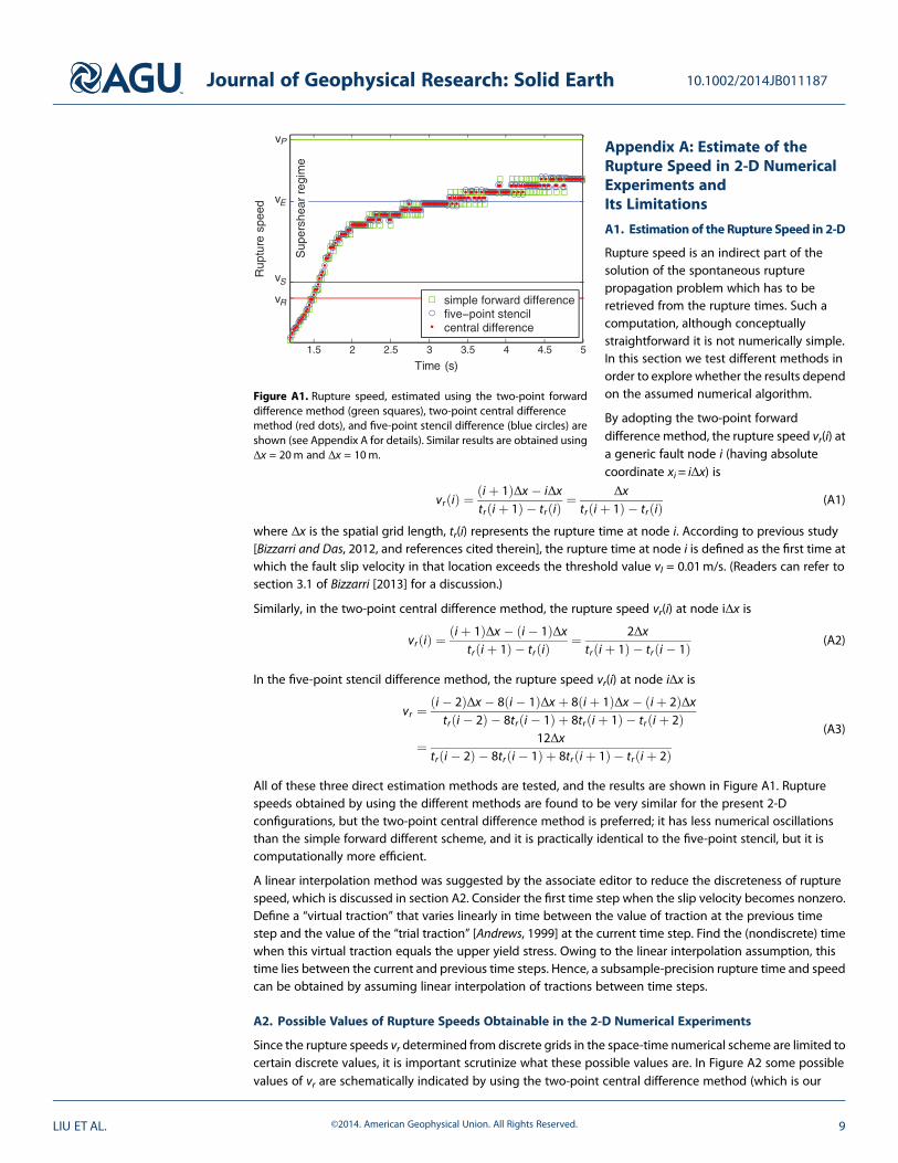
All of these three direct estimation methods are tested, and the results are shown in Figure A1. Rupturespeeds obtained by using the different methods are found to be very similar for the present 2-Dconfigurations, but the two-point central difference method is preferred; it has less numerical oscillationsthan the simple forward different scheme, and it is practically identical to the five-point stencil, but it iscomputationally more efficient.
A linear interpolation method was suggested by the associate editor to reduce the discreteness of rupturespeed, which is discussed in section A2. Consider the first time step when the slip velocity becomes nonzero.Define a “virtual traction” that varies linearly in time between the value of traction at the previous timestep and the value of the “trial traction” [Andrews, 1999] at the current time step. Find the (nondiscrete) timewhen this virtual traction equals the upper yield stress. Owing to the linear interpolation assumption, thistime lies between the current and previous time steps. Hence, a subsample-precision rupture time and speedcan be obtained by assuming linear interpolation of tractions between time steps.
A2. Possible Values of Rupture Speeds Obtainable in the 2-D Numerical Experiments
Since the rupture speeds vr determined from discrete grids in the space-time numerical scheme are limited tocertain discrete values, it is important scrutinize what these possible values are. In Figure A2 some possiblevalues of vr are schematically indicated by using the two-point central difference method (which is our
1.5 2 2.5 3 3.5 4 4.5 5
Time (s)
Rup
ture
spee
d
simple forward differencefive−point stencilcentral difference
srepuS
emig
h
errae
Figure A1. Rupture speed, estimated using the two-point forwarddifference method (green squares), two-point central differencemethod (red dots), and five-point stencil difference (blue circles) areshown (see Appendix A for details). Similar results are obtained usingΔx = 20m and Δx = 10m.
Journal of Geophysical Research: Solid Earth 10.1002/2014JB011187
LIU ET AL. ©2014. American Geophysical Union. All Rights Reserved. 9
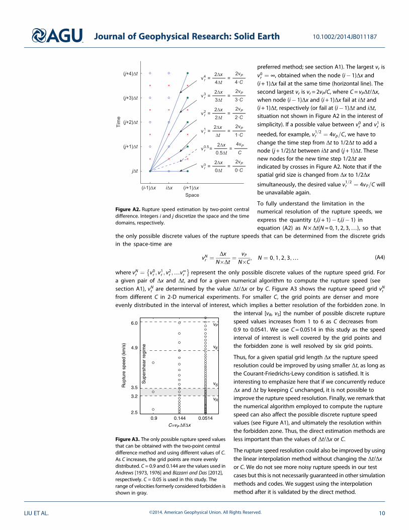
preferred method; see section A1). The largest vr is
v0r ¼ ∞, obtained when the node (i� 1)Δx and(i+ 1)Δx fail at the same time (horizontal line). Thesecond largest vr is vr= 2vP/C, where C= vPΔt/Δx,when node (i� 1)Δx and (i+ 1)Δx fail at iΔt and(i+ 1)Δt, respectively (or fail at (i� 1)Δt and iΔt,situation not shown in Figure A2 in the interest ofsimplicity). If a possible value between v0r and v1r is
needed, for example, v1=2r ¼ 4vp=C, we have tochange the time step from Δt to 1/2Δt to add anode (j+ 1/2)Δt between iΔt and (j+ 1)Δt. Thesenew nodes for the new time step 1/2Δt areindicated by crosses in Figure A2. Note that if thespatial grid size is changed from Δx to 1/2Δx
simultaneously, the desired value v1=2r ¼ 4vP=C willbe unavailable again.
To fully understand the limitation in thenumerical resolution of the rupture speeds, weexpress the quantity tr(i + 1)� tr(i� 1) inequation (A2) as N×Δt(N= 0, 1, 2, 3,…), so that
the only possible discrete values of the rupture speeds that can be determined from the discrete gridsin the space-time are
vNr ¼ ΔxN�Δt
¼ vPN�C
; N ¼ 0; 1; 2; 3;… (A4)
where vNr ¼ v0r ; v1r ; v
2r ;…v∞r
� �represent the only possible discrete values of the rupture speed grid. For
a given pair of Δx and Δt, and for a given numerical algorithm to compute the rupture speed (seesection A1), vNr are determined by the value Δt/Δx or by C. Figure A3 shows the rupture speed grid vNrfrom different C in 2-D numerical experiments. For smaller C, the grid points are denser and moreevenly distributed in the interval of interest, which implies a better resolution of the forbidden zone. In
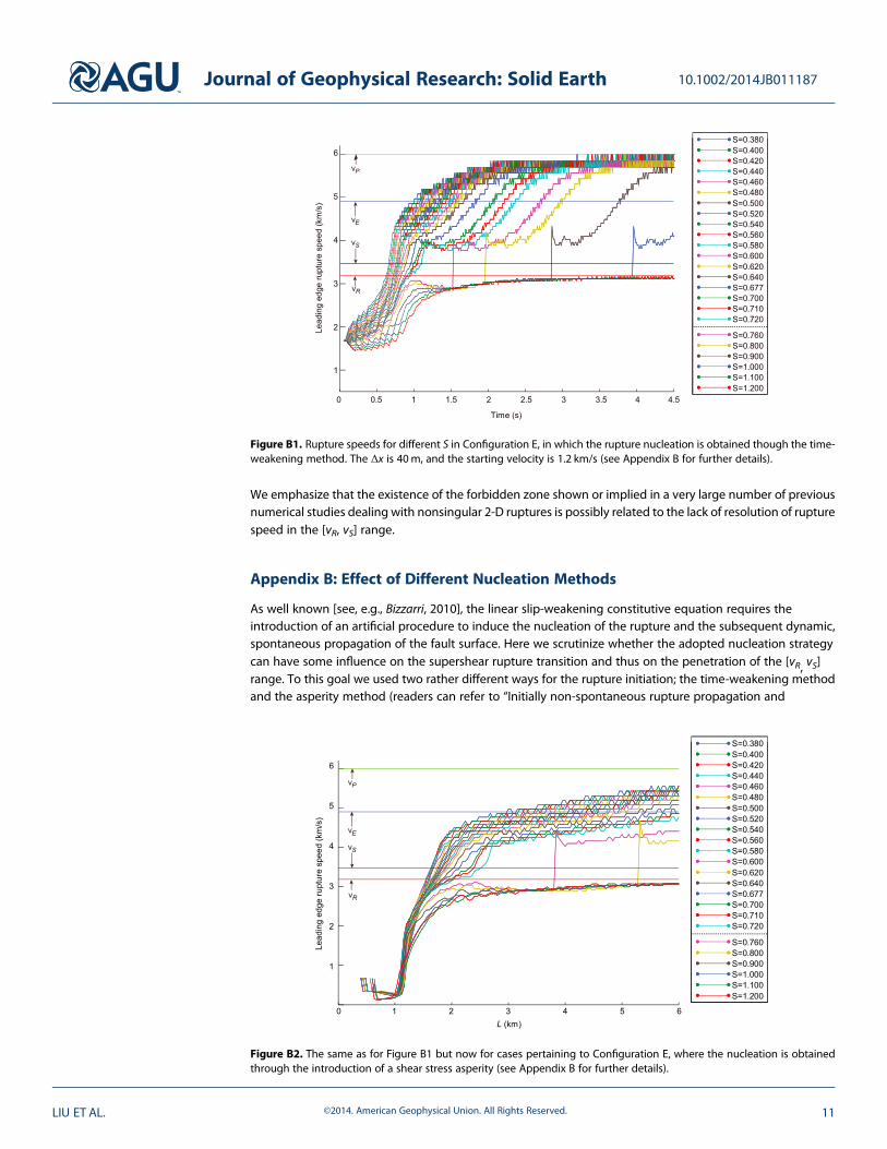
the interval [vR, vS] the number of possible discrete rupturespeed values increases from 1 to 6 as C decreases from0.9 to 0.0541. We use C=0.0514 in this study as the speedinterval of interest is well covered by the grid points andthe forbidden zone is well resolved by six grid points.
Thus, for a given spatial grid length Δx the rupture speedresolution could be improved by using smaller Δt, as long asthe Courant-Friedrichs-Lewy condition is satisfied. It isinteresting to emphasize here that if we concurrently reduceΔx and Δt by keeping C unchanged, it is not possible toimprove the rupture speed resolution. Finally, we remark thatthe numerical algorithm employed to compute the rupturespeed can also affect the possible discrete rupture speedvalues (see Figure A1), and ultimately the resolution withinthe forbidden zone. Thus, the direct estimation methods areless important than the values of Δt/Δx or C.
The rupture speed resolution could also be improved by usingthe linear interpolation method without changing the Δt/Δxor C. We do not see more noisy rupture speeds in our testcases but this is not necessarily guaranteed in other simulationmethods and codes. We suggest using the interpolationmethod after it is validated by the direct method.
C=vP Δt/Δx
Ru
ptur
esp
eed
(km
/s)
2.5
vR
vS
vE
vP
3.2
3.5
6.0
4.9
0.9 0.144 0.0514
srepuS
emiger raeh
Figure A3. The only possible rupture speed valuesthat can be obtained with the two-point centraldifference method and using different values of C.As C increases, the grid points are more evenlydistributed. C = 0.9 and 0.144 are the values used inAndrews [1973, 1976] and Bizzarri and Das [2012],respectively. C = 0.05 is used in this study. Therange of velocities formerly considered forbidden isshown in gray.
Figure A2. Rupture speed estimation by two-point centraldifference. Integers i and j discretize the space and the timedomains, respectively.
Journal of Geophysical Research: Solid Earth 10.1002/2014JB011187
LIU ET AL. ©2014. American Geophysical Union. All Rights Reserved. 10
We emphasize that the existence of the forbidden zone shown or implied in a very large number of previousnumerical studies dealing with nonsingular 2-D ruptures is possibly related to the lack of resolution of rupturespeed in the [vR, vS] range.
Appendix B: Effect of Different Nucleation Methods
As well known [see, e.g., Bizzarri, 2010], the linear slip-weakening constitutive equation requires theintroduction of an artificial procedure to induce the nucleation of the rupture and the subsequent dynamic,spontaneous propagation of the fault surface. Here we scrutinize whether the adopted nucleation strategycan have some influence on the supershear rupture transition and thus on the penetration of the [vR, vS]range. To this goal we used two rather different ways for the rupture initiation; the time-weakening methodand the asperity method (readers can refer to “Initially non-spontaneous rupture propagation and
Figure B1. Rupture speeds for different S in Configuration E, in which the rupture nucleation is obtained though the time-weakening method. The Δx is 40m, and the starting velocity is 1.2 km/s (see Appendix B for further details).
Figure B2. The same as for Figure B1 but now for cases pertaining to Configuration E, where the nucleation is obtainedthrough the introduction of a shear stress asperity (see Appendix B for further details).
Journal of Geophysical Research: Solid Earth 10.1002/2014JB011187
LIU ET AL. ©2014. American Geophysical Union. All Rights Reserved. 11
introduction of an initial shear stress asperitysections” of Bizzarri [2010], respectively, for adetailed discussion of these two strategies).The Configurations D and E (see Table 2) arerelevant to this test.
For the Configuration D, the time-weakeningmethod, a starting speed of vinit = 1.2 km/s isused, and the rupture speed curves are plottedin Figure B1. Compared to Configuration A(Figure 2), the nucleation stages have largerrupture speeds, but the spontaneous rupturebehavior is similar. In particular, we do notobserve any relevant change in thesupershear transition.
For the Configuration E, an asperity nucleationmethod is used. The stress perturbation used toinitialize the rupture is 0.5% greater than theupper yield stress. The asperity size is set to 2 LC,where LC is defined as the half-critical length inAndrews [1976] (see equation (1) of Bizzarri
[2010]), and the entire asperity is allowed to rupture at the first time step to initiate the process. The resultingrupture speed curves are plotted in Figure B2, which shows that after the nucleation stage, the spontaneousrupture behavior is similar to Figures 2 and B1.
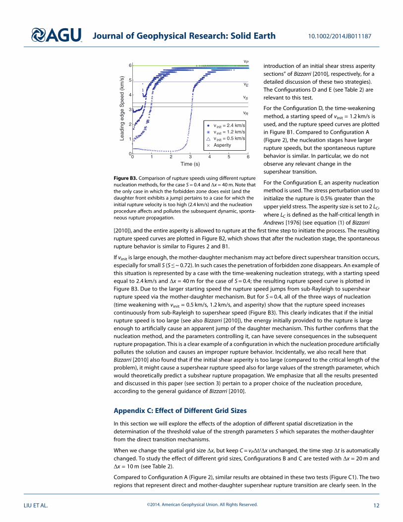
If vinit is large enough, the mother-daughter mechanismmay act before direct supershear transition occurs,especially for small S (S ≤~ 0.72). In such cases the penetration of forbidden zone disappears. An example ofthis situation is represented by a case with the time-weakening nucleation strategy, with a starting speedequal to 2.4 km/s and Δx = 40m for the case of S = 0.4; the resulting rupture speed curve is plotted inFigure B3. Due to the larger starting speed the rupture speed jumps from sub-Rayleigh to supershearrupture speed via the mother-daughter mechanism. But for S = 0.4, all of the three ways of nucleation(time weakening with vinit = 0.5 km/s, 1.2 km/s, and asperity) show that the rupture speed increasescontinuously from sub-Rayleigh to supershear speed (Figure B3). This clearly indicates that if the initialrupture speed is too large (see also Bizzarri [2010]), the energy initially provided to the rupture is largeenough to artificially cause an apparent jump of the daughter mechanism. This further confirms that thenucleation method, and the parameters controlling it, can have severe consequences in the subsequentrupture propagation. This is a clear example of a configuration in which the nucleation procedure artificiallypollutes the solution and causes an improper rupture behavior. Incidentally, we also recall here thatBizzarri [2010] also found that if the initial shear asperity is too large (compared to the critical length of theproblem), it might cause a supershear rupture speed also for large values of the strength parameter, whichwould theoretically predict a subshear rupture propagation. We emphasize that all the results presentedand discussed in this paper (see section 3) pertain to a proper choice of the nucleation procedure,according to the general guidance of Bizzarri [2010].
Appendix C: Effect of Different Grid Sizes
In this section we will explore the effects of the adoption of different spatial discretization in thedetermination of the threshold value of the strength parameters S which separates the mother-daughterfrom the direct transition mechanisms.
When we change the spatial grid size Δx, but keep C= vPΔt/Δx unchanged, the time step Δt is automaticallychanged. To study the effect of different grid sizes, Configurations B and C are tested with Δx = 20m andΔx = 10m (see Table 2).
Compared to Configuration A (Figure 2), similar results are obtained in these two tests (Figure C1). The tworegions that represent direct and mother-daughter supershear rupture transition are clearly seen. In the
0 1 2 3 4 5 60
1
2
3
4
5
6
Time (s)
Lead
ing
edge
Spe
ed (
km/s
)v init = 2.4 km/sv init = 1.2 km/sv init = 0.5 km/sAsperity
Figure B3. Comparison of rupture speeds using different rupturenucleation methods, for the case S = 0.4 and Δx = 40m. Note thatthe only case in which the forbidden zone does exist (and thedaughter front exhibits a jump) pertains to a case for which theinitial rupture velocity is too high (2.4 km/s) and the nucleationprocedure affects and pollutes the subsequent dynamic, sponta-neous rupture propagation.
Journal of Geophysical Research: Solid Earth 10.1002/2014JB011187
LIU ET AL. ©2014. American Geophysical Union. All Rights Reserved. 12
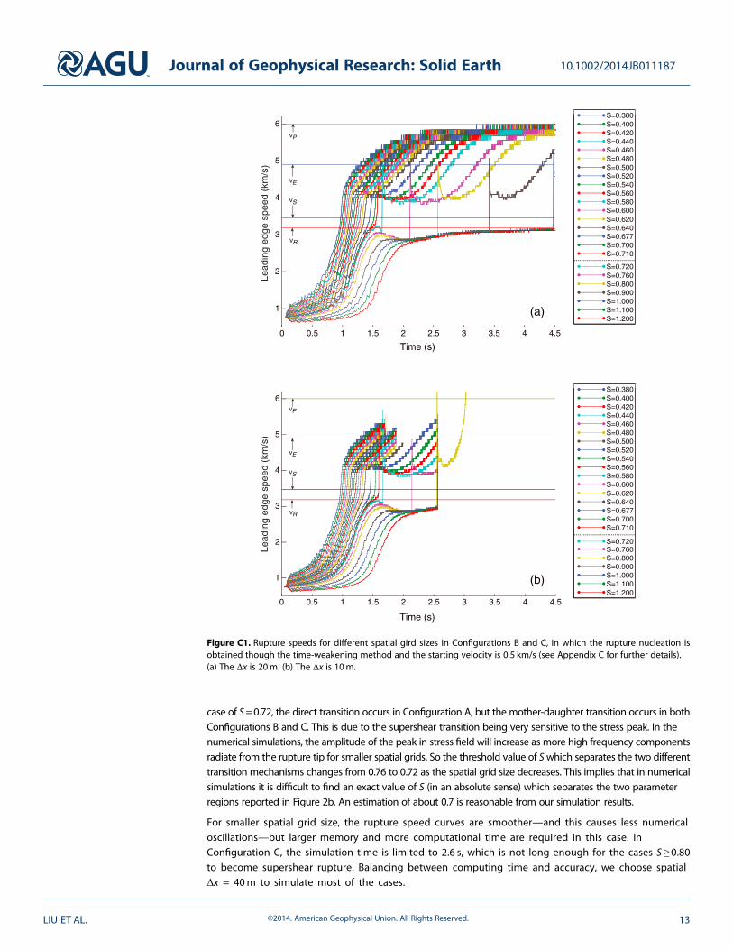
case of S=0.72, the direct transition occurs in Configuration A, but the mother-daughter transition occurs in bothConfigurations B and C. This is due to the supershear transition being very sensitive to the stress peak. In thenumerical simulations, the amplitude of the peak in stress field will increase as more high frequency componentsradiate from the rupture tip for smaller spatial grids. So the threshold value of Swhich separates the two differenttransition mechanisms changes from 0.76 to 0.72 as the spatial grid size decreases. This implies that in numericalsimulations it is difficult to find an exact value of S (in an absolute sense) which separates the two parameterregions reported in Figure 2b. An estimation of about 0.7 is reasonable from our simulation results.
For smaller spatial grid size, the rupture speed curves are smoother—and this causes less numericaloscillations—but larger memory and more computational time are required in this case. InConfiguration C, the simulation time is limited to 2.6 s, which is not long enough for the cases S ≥ 0.80to become supershear rupture. Balancing between computing time and accuracy, we choose spatialΔx = 40m to simulate most of the cases.
Time (s)
1
2
3
4
5
6
vR
vS
vE
vP
Lead
ing
edge
spe
ed (
km/s
)
0 0.5 1 1.5 2 2.5 3 3.5 4 4.5
0 0.5 1 1.5 2 2.5 3 3.5 4 4.5
(a)
1
2
3
4
5
6
Lead
ing
edge
spe
ed (
km/s
)
Time (s)
(b)
S=0.380S=0.400S=0.420S=0.440S=0.460S=0.480S=0.500S=0.520S=0.540S=0.560S=0.580S=0.600S=0.620S=0.640S=0.677S=0.700S=0.710
S=0.720S=0.760S=0.800S=0.900S=1.000S=1.100S=1.200
S=0.380S=0.400S=0.420S=0.440S=0.460S=0.480S=0.500S=0.520S=0.540S=0.560S=0.580S=0.600S=0.620S=0.640S=0.677S=0.700S=0.710
S=0.720S=0.760S=0.800S=0.900S=1.000S=1.100S=1.200
vR
vS
vE
vP
Figure C1. Rupture speeds for different spatial gird sizes in Configurations B and C, in which the rupture nucleation isobtained though the time-weakening method and the starting velocity is 0.5 km/s (see Appendix C for further details).(a) The Δx is 20m. (b) The Δx is 10m.
Journal of Geophysical Research: Solid Earth 10.1002/2014JB011187
LIU ET AL. ©2014. American Geophysical Union. All Rights Reserved. 13
ReferencesAagaard, B. T., and T. H. Heaton (2004), Near-source ground motions from simulations of sustained intersonic and supersonic fault ruptures,
Bull. Seismol. Soc. Am., 94, 2064–2078.Abraham, F. F., and H. Gao (2000), How fast can cracks propagate?, Phys. Rev. Lett., 84, 3113–3116.Andrews, D. J. (1973), A numerical study of tectonic stress release by underground explosions, Bull. Seismol. Soc. Am., 63(4), 1375–1391.Andrews, D. J. (1976), Rupture velocity of plane strain shear cracks, J. Geophys. Res., 81(32), 5679–5687, doi:10.1029/JB081i032p05679.Andrews, D. J. (1985), Dynamic plane-strain shear rupture with a slip-weakening friction law calculated by a boundary integral method, Bull.
Seismol. Soc. Am., 75(1), 1–21.Andrews, D. J. (1999), Test of two methods for faulting in finite-difference calculations, Bull. Seismol. Soc. Am., 89(4), 931–937.Aochi, H., E. Fukuyama, and M. Matsu’ura (2000), Spontaneous rupture propagation on a non–planar fault in 3D elastic medium, Pure Appl.
Geophys., 157, 2003–2027, doi:10.1007/PL00001072.Archuleta, R. J. (1984), A faulting model for the 1979 Imperial Valley earthquake, J. Geophys. Res., 89(B6), 4559–4585, doi:10.1029/
JB089iB06p04559.Bhat, H. S., R. Dmowska, G. C. King, Y. Klinger, and J. R. Rice (2007), Off-fault damage patterns due to supershear ruptures with application to
the 2001 Mw 8.1 Kokoxili (Kunlun) Tibet earthquake, J. Geophys. Res., 112, B06301, doi:10.1029/2006JB004425.Bizzarri, A. (2010), How to promote earthquake ruptures: Different nucleation strategies in a dynamic model with slip-weakening friction,
Bull. Seismol. Soc. Am., 100(3), 923–940, doi:10.1785/0120090179.Bizzarri, A. (2011), On the deterministic description of earthquakes, Rev. Geophys., 49, RG3002, doi:10.1029/2011RG000356.Bizzarri, A. (2013), Calculation of the local rupture speed of dynamically propagating earthquakes, Ann. Geophys., 56(5), S0560, doi:10.4401/
ag-6279.Bizzarri, A., and M. Cocco (2005), 3D dynamic simulations of spontaneous rupture propagation governed by different constitutive laws with
rake rotation allowed, Ann. Geophys., 48(2), 279–299.Bizzarri, A., and S. Das (2012), Mechanics of 3-D shear cracks between Rayleigh and shear wave rupture speeds, Earth Planet. Sci. Lett.,
357-358, 397–404, doi:10.1016/j.epsl.2012.09.053.Bizzarri, A., and P. Spudich (2008), Effects of supershear rupture speed on the high-frequency content of S waves investigated using spon-
taneous dynamic rupture models and isochrone theory, J. Geophys. Res., 113, B05304, doi:10.1029/2007JB005146.Bizzarri, A., M. Cocco, D. Andrews, and E. Boschi (2001), Solving the dynamic rupture problem with different numerical approaches and
constitutive laws, Geophys. J. Int., 144, 656–678, doi:10.1046/j.1365-246x.2001.01363.x.Bizzarri, A., E. M. Dunham, and P. Spudich (2010), Coherence of Mach fronts during heterogeneous supershear earthquake rupture propa-
gation: Simulations and comparison with observations, J. Geophys. Res., 115, B08301, doi:10.1029/2009JB006819.Bouchon, M., and M. Vallée (2003), Observation of long supershear rupture during the magnitude 8.1 Kunlunshan earthquake, Science,
301(5634), 824–826.Bouchon, M., M. P. Bouin, H. Karabulut, M. N. Toksöz, M. Dietrich, and A. J. Rosakis (2001), How fast is rupture during an earthquake? New
insights from the 1999 Turkey earthquakes, Geophys. Res. Lett., 28(14), 2723–2726, doi:10.1029/2001GL013112.Broberg, K. B. (1994), Intersonic bilateral slip, Geophys. J. Int., 119, 706–714.Broberg, K. B. (1995), Intersonic mode II crack expansion, Arch. Mech., 47, 859–871.Broberg, K. B. (1999), Cracks and Fracture, Academic Press, London.Burridge, R. (1973), Admissible speeds for plane-strain self-similar shear cracks with friction but lacking cohesion, Geophys. J. Int., 35(4), 439–455.Burridge, R., G. Conn, and L. B. Freund (1979), The stability of a rapid mode II shear crack with finite cohesive traction, J. Geophys. Res., 84(B5),
2210–2222, doi:10.1029/JB084iB05p02210.Das, S. (1976), A numerical study of rupture propagation and earthquake source mechanism, PhD thesis, Dep. of Earth and Planetary
Sciences, Massachusetts Institute of Technology, Mass.Das, S., and K. Aki (1977), A numerical study of two-dimensional spontaneous rupture propagation, Geophys. J. Int., 50(3), 643–668.Dunham, E. M. (2007), Conditions governing the occurrence of supershear ruptures under slip-weakening friction, J. Geophys. Res., 112,
B07302, doi:10.1029/2006JB004717.Dunham, E. M., and R. J. Archuleta (2004), Evidence for a supershear transient during the 2002 Denali Fault earthquake, Bull. Seismol. Soc. Am.,
94(6B), S256–S268.Ellsworth, W., M. Celebi, J. Evans, E. Jensen, R. Kayen, M. Metz, D. Nyman, J. Roddick, P. Spudich, and C. Stephens (2004), Near-field ground
motion of the 2002 Denali Fault, Alaska, earthquake recorded at Pump Station 10, Earthquake Spectra, 20(3), 597–615.Festa, G., and J. P. Vilotte (2006), Influence of the rupture initiation on the intersonic transition: Crack-like versus pulse-like modes, Geophys.
Res. Lett., 33, L15320, doi:10.1029/2006GL026378.Fliss, S., H. S. Bhat, R. Dmowska, and J. R. Rice (2005), Fault branching and rupture directivity, J. Geophys. Res., 110, B06312, doi:10.1029/
2004JB003368.Freund, L. B. (1979), The mechanics of dynamic shear crack propagation, J. Geophys. Res., 84(B5), 2199–2209, doi:10.1029/JB084iB05p02199.Geubelle, P. H., and D. V. Kubair (2001), Intersonic crack propagation in homogeneous media under shear-dominated loading: Numerical
analysis, J. Mech. Phys. Solids, 49(3), 571–587.Hamano, Y. (1974), Dependence of rupture-time history on heterogeneous distribution of stress and strength on fault plane (abstract), Eos
Trans. AGU, 55, 352.Ida, Y. (1972), Cohesive force across the tip of a longitudinal-shear crack and Griffith’s specific surface energy, J. Geophys. Res., 77(20),
3796–3805, doi:10.1029/JB077i020p03796.Kame, N., J. R. Rice, and R. Dmowska (2003), Effects of prestress state and rupture velocity on dynamic fault branching, J. Geophys. Res.,
108(B5), 2265, doi:10.1029/2002JB002189.Liu, Y., and N. Lapusta (2008), Transition of mode II cracks from sub-Rayleigh to intersonic speeds in the presence of favorable heterogeneity,
J. Mech. Phys. Solids, 56(1), 25–50.Lu, X., N. Lapusta, and A. J. Rosakis (2007), Pulse-like and crack-like ruptures in experiments mimicking crustal earthquakes, Proc. Natl. Acad.
Sci. U.S.A., 104(48), 18,931–18,936.Lu, X., N. Lapusta, and A. J. Rosakis (2009), Analysis of supershear transition regimes in rupture experiments: The effect of nucleation con-
ditions and friction parameters, Geophys. J. Int., 177(2), 717–732.Mitchell, A. R. (1976), Computational Methods in Partial Differential Equations, Wiley, New York.Olsen, K. B., R. Madariaga, and R. J. Archuleta (1997), Three-dimensional dynamic simulation of the 1992 Landers earthquake, Science,
278(5339), 834–838.
Journal of Geophysical Research: Solid Earth 10.1002/2014JB011187
LIU ET AL. ©2014. American Geophysical Union. All Rights Reserved. 14
AcknowledgmentsC.L. is supported by the NewtonInternational Fellowship 2012 of TheRoyal Society (NF120809). The authorswould like to thank the Associate Editorand two anonymous reviewers for themany interesting comments and sug-gestions which improved and clarifiedthe paper.
Passelègue, F. X., A. Schubnel, S. Nielsen, H. S. Bhat, and R. Madariaga (2013), From sub-Rayleigh to supershear ruptures during stick-slipexperiments on crustal rocks, Science, 340(6137), 1208–1211.
Poliakov, A. N. B., R. Dmowska, and J. R. Rice (2002), Dynamic shear rupture interactions with fault bends and off-axis secondary faulting,J. Geophys. Res., 107(B11), 2295, doi:10.1029/2001JB000572.
Robinson, D. P., C. Brough, and S. Das (2006), The Mw 7.8, 2001 Kunlunshan earthquake: Extreme rupture speed variability and effect of faultgeometry, J. Geophys. Res., 111, B08303, doi:10.1029/2005JB004137.
Robinson, D. P., S. Das, and M. P. Searle (2010), Earthquake fault superhighways, Tectonophysics, 493(3), 236–243.Rosakis, A. J. (2002), Intersonic shear cracks and fault ruptures, Adv. Phys., 51(4), 1189–1257.Rosakis, A. J., O. Samudrala, and D. Coker (1999), Cracks faster than the shear wave speed, Science, 284(5418), 1337–1340.Rosakis, A., K. Xia, G. Lykotrafitis, and H. Kanamori (2007), Dynamic shear rupture in frictional interfaces: Speeds, directionality and modes,
Treatise Geophys., 4, 153–192.Vallée, M., M. Landès, N. M. Shapiro, and Y. Klinger (2008), The 14 November 2001 Kokoxili (Tibet) earthquake: High-frequency seismic
radiation originating from the transitions between sub-Rayleigh and supershear rupture velocity regimes, J. Geophys. Res., 113, B07305,doi:10.1029/2007JB005520.
Xia, K., A. J. Rosakis, and H. Kanamori (2004), Laboratory earthquakes: The sub-Rayleigh-to-supershear rupture transition, Science, 303(5665),1859–1861.
Xia, K., A. J. Rosakis, H. Kanamori, and J. R. Rice (2005), Laboratory earthquakes along inhomogeneous faults: Directionality and supershear,Science, 308, 681–684.
Journal of Geophysical Research: Solid Earth 10.1002/2014JB011187
LIU ET AL. ©2014. American Geophysical Union. All Rights Reserved. 15