Embed Size (px)
Citation preview
Abstract
Progress toward Searching for Electron Electric Dipole
Moment using PbO
Yong Jiang
2008
Observation of a non-zero electron electric dipole moment (EDM) will be explicit evidence
for physics beyond the Standard Model. There is significant interest in developing exper
iments that can probe beyond the current limits for the electron EDM. An experiment
to look for the EDM of the electron using the metastable a(l)(3S+) state of the PbO
molecule has been implemented at Yale University. We populate the a(l) [3S+] state of
208PbO using laser-microwave double resonance, and we detect fluorescence, using quan
tum beat spectroscopy to extract minute frequency changes due to the electron EDM. The
experimental method and setup will be described in this thesis. We have demonstrated the
ability to manipulate the internal molecular state in such a way as to produce the desired
states for our EDM experiment. Efforts were carried out to optimize the state excitation
efficiency using an adiabatic following scheme. We performed various experiments to con
firm our understanding of molecular state evolution dynamics in a variety of experimental
configurations. Our experiment improved the accuracy of previously measured molecular
constants of PbO, which cast light on the feasibility of future systematic error checking
and reduction. Due to various technical issues, the sensitivity to an electron EDM in this
generation of EDM experiment is far less than expected. Two novel proposals for a second
generation EDM experiment are considered.

Progress toward Searching for Electron Electric
Dipole Moment using PbO
A Dissertation Presented to the Faculty of the Graduate School
of Yale University
in Candidacy for the Degree of Doctor of Philosophy
by Yong Jiang
Dissertation Director: David DeMille
May 2008

UMI Number: 3317137
INFORMATION TO USERS
The quality of this reproduction is dependent upon the quality of the copy
submitted. Broken or indistinct print, colored or poor quality illustrations and
photographs, print bleed-through, substandard margins, and improper
alignment can adversely affect reproduction.
In the unlikely event that the author did not send a complete manuscript
and there are missing pages, these will be noted. Also, if unauthorized
copyright material had to be removed, a note will indicate the deletion.
®
UMI UMI Microform 3317137
Copyright 2008 by ProQuest LLC.
All rights reserved. This microform edition is protected against
unauthorized copying under Title 17, United States Code.
ProQuest LLC 789 E. Eisenhower Parkway
PO Box 1346 Ann Arbor, Ml 48106-1346
Copyright © 2008 by Yong Jiang
All rights reserved.
Acknowledgements
It is my pleasure to express my thanks to the many people who made this thesis possible.
In the first place I would like to gratefully and sincerely thank my research advisor,
Professor David DeMille, for his advice, guidance, understanding, and patience. With
his enthusiasm, his truly scientist intuition, his inspiration, and his great efforts to explain
things clearly and simply, he provided me sound advice, great ideas, genuine encouragement
and support throughout my PhD life. I could not have imagined having a better advisor
and mentor for my PhD. I am greatly indebted to him more than he knows.
I gratefully acknowledge all the members of my thesis committee for their accessibility
and valuable advice.
Collective and individual acknowledgments are also owed to my colleagues at Yale.
Best regards to all members of Prof. DeMille's research group for their friendship and help.
Especially I gratefully acknowledge Sarah Bickman, Paul Hamilton and Amar Vutha who
provided me with one of the most comfortable working places I have ever had. I would like
to extend my sincerest thanks to my co-workers David Kawall, Richard Paolino, Prederik
Bay, Valmiki Prasad, and etc. There are many others who contributed to this work.
Sidney Cahn offered advice on technical issues and provided some much needed humor
and entertainment in what could have otherwise been a somewhat stressful laboratory
environment. Vincent Bernardo and the entire Gibbs Machine Shop did great jobs on
metal machining. I am grateful to all of the faculty and staff in Department of Physics at
Yale, for assisting me in many different ways and many other issues for their hard work,
iii
expertise and patience.
I am especially indebted to my wife Yi Wang, who has continually offered her ardent
love, selfless dedication, and persistent confidence in me. Her staunch support, quiet pa
tience, and unwavering faith have taken the load off my shoulder. And The birth of our
beautiful baby boy Leon brings an additional and enjoyable dimension to our life. I thank
my parents for their faith in me and allowing me to be as ambitious as I wanted. Also, I
thank Yi's parents. They provided Yi and me with unending encouragement and support.
I wish to thank my entire extended family for providing a loving environment for me.
Finally, I would like to thank everybody who was important to the successful realization
of thesis, as well as expressing my apology that I could not mention personally one by one.
iv
Contents
Acknowledgements iii
1 Introduction 1
1.1 General Introduction to EDM Experiments 1
1.1.1 Motivation for Searches for EDM 1
1.2 Electron EDM Experiments with Atoms or Molecules 4
1.2.1 Atomic EDM Experiments 5
1.2.2 EDM Enhancement in Diatomic Molecules 7
2 Probing the Electron EDM using PbO 10
2.1 Principal Properties of the PbO a(l) State 10
2.2 Experimental Method 15
2.3 Experimental Setup 19
2.4 Quantum Beat Spectroscopy in Fluorescence 22
2.4.1 Quantum Beats 23
2.4.2 Data Analysis 25
2.5 Statistical Sensitivity of EDM Experiment 33
2.6 Overview of Systematic Effects 34
2.6.1 Applied External Field 35
2.6.2 Leakage Current Effects 39
2.6.3 The Internal Co-Magnetometer 40
v
3 Experimental Apparatus 43
3.1 Development of the Vapor Cell 44
3.1.1 Electrodes with Guard Rings 46
3.1.2 Leakage Current Suppression 51
3.2 Development of the Oven 54
3.3 Eddy Current Suppression 57
3.4 Plunger 69
3.5 Non-Magnetic BNC Feedthrough 71
3.6 Magnetic Shield and Magnetic Coils 72
3.7 High Voltage Amplifier 76
3.7.1 Circuit Design 77
3.7.2 Performance Measurement 79
3.8 Laser Excitation and Fluorescence Detection 81
3.8.1 Laser Excitation 81
3.8.2 Beam Homogenizer 82
3.8.3 Fluorescence Collection 84
3.8.4 Fluorescence Detection 86
4 Molecular State Preparation 89
4.1 Previous Attempts using RF Excitation 89
4.1.1 RF Coherent Excitation 91
4.1.2 RF Experimental Setup 93
4.1.3 RF Transition Efficiency 97
4.2 State Population Transfer using Microwave Excitaion 102
4.2.1 a(l) J=2 Rotational State 102
4.2.2 Microwave Coherent Excitation 105
4.2.3 Population Transfer Path 106
4.2.4 Experimental Setup 110
vi
4.2.5 State Preparation by Rabi Oscillation 113
4.3 Adiabatic Following in Microwave Excitation 120
4.3.1 Adiabatic Following 121
4.3.2 Generalized Landau-Zener Model 123
4.3.3 Adiabatic Following Experiment 130
4.3.4 Double Pulsed Adiabatic Following 133
4.3.5 Technical Concern 137
4.3.6 Conclusion 138
5 Measurement of Molecular Parameters 139
5.1 Zeeman Effect Measurement 139
5.2 Stark Effect Measurement 142
5.3 Quantum Beats in Electric Field 143
5.4 Conclusion 155
6 Current Status and Future Directions 156
6.1 Current Status 156
6.2 Future Direction I: Microwave Absorption 162
6.2.1 General Description 162
6.2.2 Absorption Cross Section 162
6.2.3 Signal to Noise 169
6.3 Future Direction II: Beam EDM 172
6.3.1 Cold Beam Experiment 172
6.3.2 Candidates for Cold Molecular Beam EDM Experiment 173
vii
List of Figures
2.1 a(l) J = l State in the Electric Field 16
2.2 Schematic Diagram of Energy Levels of a(l) 3T,^ PbO 17
2.3 Schematic of PbO EDM Experiment Setup 20
2.4 Energy Level Diagram for Quantum Beat 24
2.5 Typical Waveform of Quantum Beat Fluorescence Signals 26
3.1 Vapor Cell and its Cut View 44
3.2 Electric Field in the Cell 48
3.3 Electric Field Inhomogeneity in the Cell 49
3.4 Optimal Voltage Ratio 50
3.5 Bent Quartz Tube and Corner Bracket 53
3.6 Oven inside the Heat Shield 55
3.7 Heater Currents 58
3.8 Network Model of Eddy Current 60
3.9 Heater Current and Frequency Spectrum 61
3.10 Current Loop above a Metal Sheet 63
3.11 Plunger System 70
3.12 Non-Magnetic BNC Feedthrough 73
3.13 Magnetic Shields and Aluminum Supports 75
3.14 Schematic Diagram of High Voltage Amplifier 77
3.15 Performance Measurement of High Voltage Amplifier 80
viii
3.16 Engineered Diffuser 83
3.17 Winston Cones and Support 84
3.18 Schematic Diagram of a Winston Cone 85
3.19 Simulation and Sample of Winston Cone 86
3.20 Simplified Model for Photodiode Transimpedance Amplifier 87
4.1 RF Excitation Scheme and Mechanism for Systematic Suppression 90
4.2 V-Shape Level Structure and Transition Probability 92
4.3 RF Coil and RF Network Scheme 94
4.4 Transmission Line Model 95
4.5 Beat Disappearance Experiment using RF transition 98
4.6 RF Excitation Experiment Result 100
4.7 RF-Excited Beat with Various Guard Ring Voltage 101
4.8 Schematic Diagram of Energy Levels of PbO 103
4.9 Molecular Polarization in Electric Field 105
4.10 Related Level Structure and Transition Probability 107
4.11 Population Transfer Path via J=2 Level 109
4.12 Microwave Experimental Setup 110
4.13 Calibration of Microwave Amplifier Gain and Insertion Loss of Experimental
Apparatus 112
4.14 Transition by Vertical Polarized MW at Zero E Field 114
4.15 Interference of J = l Beat and J=2 Beat 115
4.16 Transition by Vertical Polarized MW in External E Field 116
4.17 Transition Driven by Horizontally Polarized MW 118
4.18 Parametrization of Generalized Landau-Zener Model 124
4.19 Fourier Transform of Frequency-Modulated Sinusoid Pulse 125
4.20 Generalized Landau-Zener Model 128
ix
4.21 Transition Probability at Different Frequency Deviation and Power using
Adiabatic Following 129
4.22 Typical Result using Adiabatic Following 131
4.23 Optimization of Frequency Sweeping Rate 133
4.24 Beat Amplitude at Various Sweeping Rates 134
4.25 Selective Preparation of EDM States using MW Adiabatic Following . . . . 136
5.1 Beat Frequency Change with RF Transition 141
5.2 Resonance Frequency Dependence on Applied Voltage 143
5.3 Beat Lifetime at Level Crossing 145
5.4 J = l Level Crossing in Electric Field 146
5.5 a(l) J = l Beat Amplitude in Electric Field 148
5.6 Beat Amplitude Changes as Electric Field Increases 150
5.7 a(l) J=2 Beat Amplitude in Low Electric Field 151
5.8 Calculated Quantum Beat Frequency Change in the Electric Field 152
5.9 Interference between beats at High Electric Field and High Magnetic Field 154
6.1 PbO Spectrum 158
6.2 Level Scheme for Absorption of Horizontally Polarized Microwave 163
6.3 Current Microwave Absorption Setup 166
6.4 Level Scheme for Absorption of Vertically Polarized Microwave 168
6.5 MW Absorption Setup 170
6.6 Electronic States in HfO and ThO 175
x

List of Tables
1.1 Calculated P,T-odd coefficients of polar diatomic paramagnetic molecules
and molecular ions 9
3.1 Signal to Noise Ratio of Detectors 88
4.1 RF Field Strength at Various Frequencies 96
6.1 Expected and Actual Increase of the Signal, Contrast and Backgrounds . . 160
6.2 Frequency Resolution and eEDM Sensitivities in Beam Experiment 174
XI
Chapter 1
Introduction
1.1 General Introduction to EDM Experiments
Although a half-century of devoted efforts have yielded only null results, there is still
significant interest in developing experiments that can probe beyond the current limits for
the electron electric dipole moment (EDM). Observation of a non-zero electron EDM will
be explicit evidence for physics beyond the Standard Model.
1.1.1 Motivation for Searches for EDM
Symmetries are essential to modern physics. They are related to conservation laws and in
variants to the dynamics of the world. A broken symmetry will be the key to revealing novel
particles or interactions. A non-zero electric dipole moment of a non-degenerate quantum
system directly violates both parity and time-reversal symmetries. Further, through the
CPT theorem, an EDM implies a breakdown of CP symmetry. A non-degenerate system
in its rest frame can be described by the internal angular momentum j . The non-zero
projection d of an EDM along (or opposite to) j is of most interest to theorists, because a
parity transformation reverses the polar vector d yet leaves unchanged the axial vector j ,
yielding the parity symmetry violation; under time reversal transformation, d stays intact,
and j changes sign, so that time reversal is also broken.
1
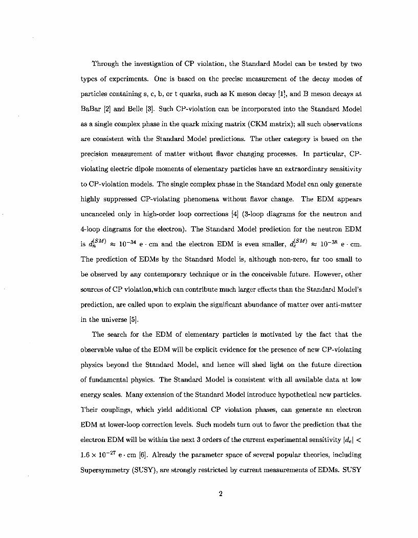
Through the investigation of CP violation, the Standard Model can be tested by two
types of experiments. One is based on the precise measurement of the decay modes of
particles containing s, c, b, or t quarks, such as K meson decay [1], and B meson decays at
BaBar [2] and Belle [3]. Such CP-violation can be incorporated into the Standard Model
as a single complex phase in the quark mixing matrix (CKM matrix); all such observations
are consistent with the Standard Model predictions. The other category is based on the
precision measurement of matter without flavor changing processes. In particular, CP-
violating electric dipole moments of elementary particles have an extraordinary sensitivity
to CP-violation models. The single complex phase in the Standard Model can only generate
highly suppressed CP-violating phenomena without flavor change. The EDM appears
uncanceled only in high-order loop corrections [4] (3-loop diagrams for the neutron and
4-loop diagrams for the electron). The Standard Model prediction for the neutron EDM
is dn « 10~34 e • cm and the electron EDM is even smaller, de ' « 10~38 e • cm.
The prediction of EDMs by the Standard Model is, although non-zero, far too small to
be observed by any contemporary technique or in the conceivable future. However, other
sources of CP violation,which can contribute much larger effects than the Standard Model's
prediction, are called upon to explain the significant abundance of matter over anti-matter
in the universe [5].
The search for the EDM of elementary particles is motivated by the fact that the
observable value of the EDM will be explicit evidence for the presence of new CP-violating
physics beyond the Standard Model, and hence will shed light on the future direction
of fundamental physics. The Standard Model is consistent with all available data at low
energy scales. Many extension of the Standard Model introduce hypothetical new particles.
Their couplings, which yield additional CP violation phases, can generate an electron
EDM at lower-loop correction levels. Such models turn out to favor the prediction that the
electron EDM will be within the next 3 orders of the current experimental sensitivity \de\ <
1.6 x 10 - 2 7 e • cm [6]. Already the parameter space of several popular theories, including
Supersymmetry (SUSY), are strongly restricted by current measurements of EDMs. SUSY
2
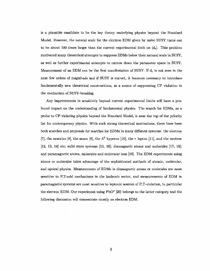
is a plausible candidate to be the key theory underlying physics beyond the Standard
Model. However, the natural scale for the electron EDM given by naive SUSY turns out
to be about 100 times larger than the current experimental limit on \de\. This problem
motivated many theoretical attempts to suppress EDMs below their natural scale in SUSY,
as well as further experimental attempts to narrow down the parameter space in SUSY.
Measurement of an EDM can be the first manifestation of SUSY. If de is not seen in the
next few orders of magnitude and if SUSY is correct, it becomes necessary to introduce
fundamentally new theoretical constructions, as a means of suppressing CP violation in
the mechanism of SUSY-breaking.
Any improvements in sensitivity beyond current experimental limits will have a pro
found impact on the understanding of fundamental physics. The search for EDMs, as a
probe to CP-violating physics beyond the Standard Model, is near the top of the priority
list for contemporary physics. With such strong theoretical motivations, there have been
both searches and proposals for searches for EDMs in many different systems: the electron
[7], the neutrino [8], the muon [9], the A0 hyperon [10], the T lepton [11], and the neutron
[12, 13, 14] etc; solid state systems [15, 16]; diamagnetic atoms and molecules [17, 18];
and paramagnetic atoms, molecules and molecular ions [19]. The EDM experiments using
atoms or molecules takes advantage of the sophisticated methods of atomic, molecular,
and optical physics. Measurements of EDMs in diamagnetic atoms or molecules are most
sensitive to P,T-odd mechanisms in the hadronic sector, and measurements of EDM in
paramagnetic systems are most sensitive to leptonic sources of P,T-violation, in particular
the electron EDM. Our experiment using PbO* [20] belongs to the latter category and the
following discussion will concentrate mostly on electron EDM.
3
1.2 Electron EDM Experiments with Atoms or Molecules
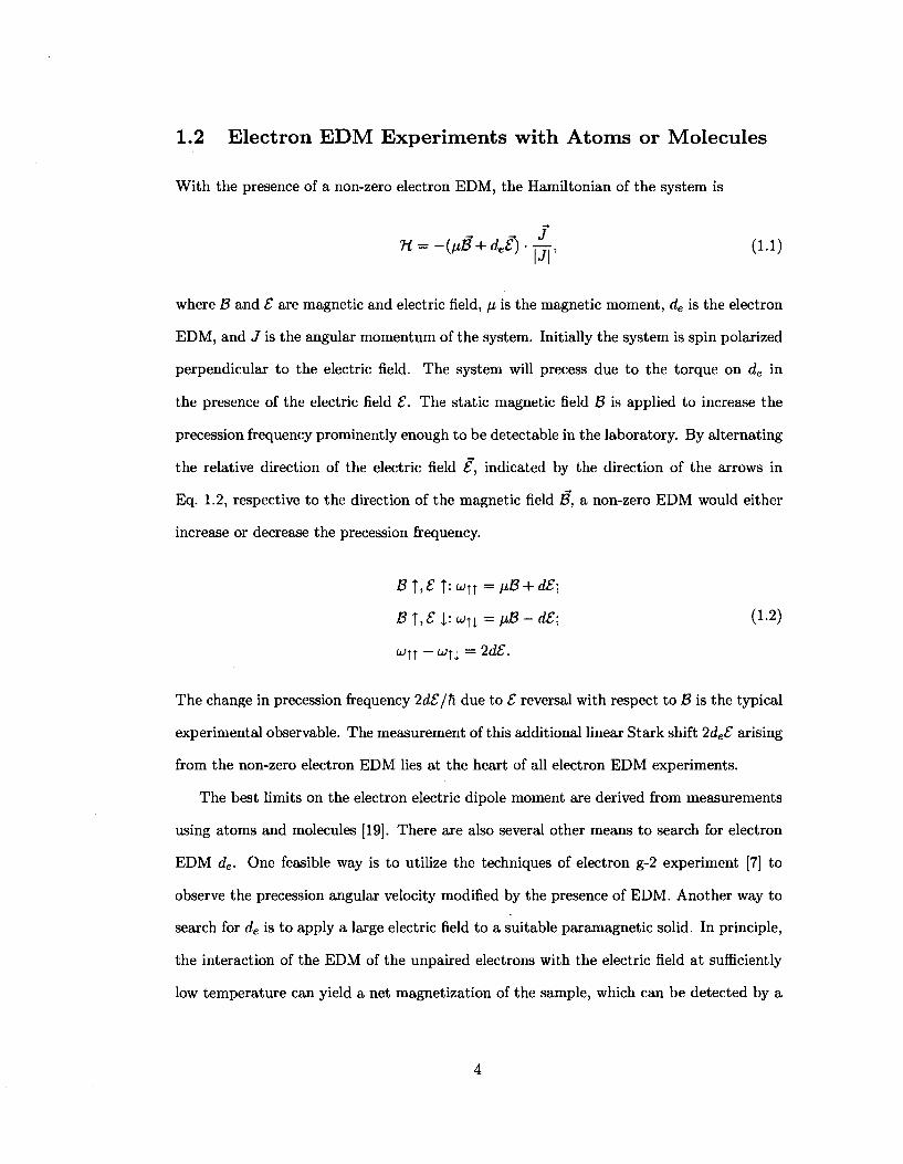
With the presence of a non-zero electron EDM, the Hamiltonian of the system is
« = -(/*£+de^-gp (1.1)
where B and £ are magnetic and electric field, \x is the magnetic moment, de is the electron
EDM, and J is the angular momentum of the system. Initially the system is spin polarized
perpendicular to the electric field. The system will precess due to the torque on de in
the presence of the electric field £. The static magnetic field B is applied to increase the
precession frequency prominently enough to be detectable in the laboratory. By alternating
the relative direction of the electric field £, indicated by the direction of the arrows in
Eq. 1.2, respective to the direction of the magnetic field B, a non-zero EDM would either
increase or decrease the precession frequency.
BT»£T:wTT = A*8 + d£;
B1,£l:un = iJ&-d£; (1-2)
u>f j - u>n = 2d£.
The change in precession frequency 2d£/h due to £ reversal with respect to B is the typical
experimental observable. The measurement of this additional linear Stark shift 2de£ arising
from the non-zero electron EDM lies at the heart of all electron EDM experiments.
The best limits on the electron electric dipole moment are derived from measurements
using atoms and molecules [19]. There are also several other means to search for electron
EDM de. One feasible way is to utilize the techniques of electron g-2 experiment [7] to
observe the precession angular velocity modified by the presence of EDM. Another way to
search for de is to apply a large electric field to a suitable paramagnetic solid. In principle,
the interaction of the EDM of the unpaired electrons with the electric field at sufficiently
low temperature can yield a net magnetization of the sample, which can be detected by a
4
superconducting quantum interference device (SQUID) magnetometer [15]. Alternatively,
application of an external magnetic field to a suitable ferromagnetic solid can yield an
EDM-induced electric polarization of the sample, which is detectable in principle by ultra
sensitive charge measurement techniques [16]. Another approach has been proposed, in
which a sufficiently large external electric field applied to a gaseous sample of diamagnetic
diatomic molecules can generate an observable P,T-odd magnetization [21].
1.2.1 Atomic E D M Experiments
A permanent atomic EDM arises from the intrinsic EDMs of unpaired valence electrons,
neutrons, and protons. However, Schiff's theorem [22] states that an atom or molecule
cannot exhibit a linear Stark effect to first order in the EDM of any constituent particle,
in the limit of non-relativistic quantum mechanics. Since a neutral atom is not accelerated
in an external electric field, the average force on each charged particle in the atom must be
zero, such that, in the non-relativistic limit only including electrostatic force, the average
electric field at each charged particle must vanish. It follows that the externally applied
static electric field must be canceled, on average, by the internal polarizing field.
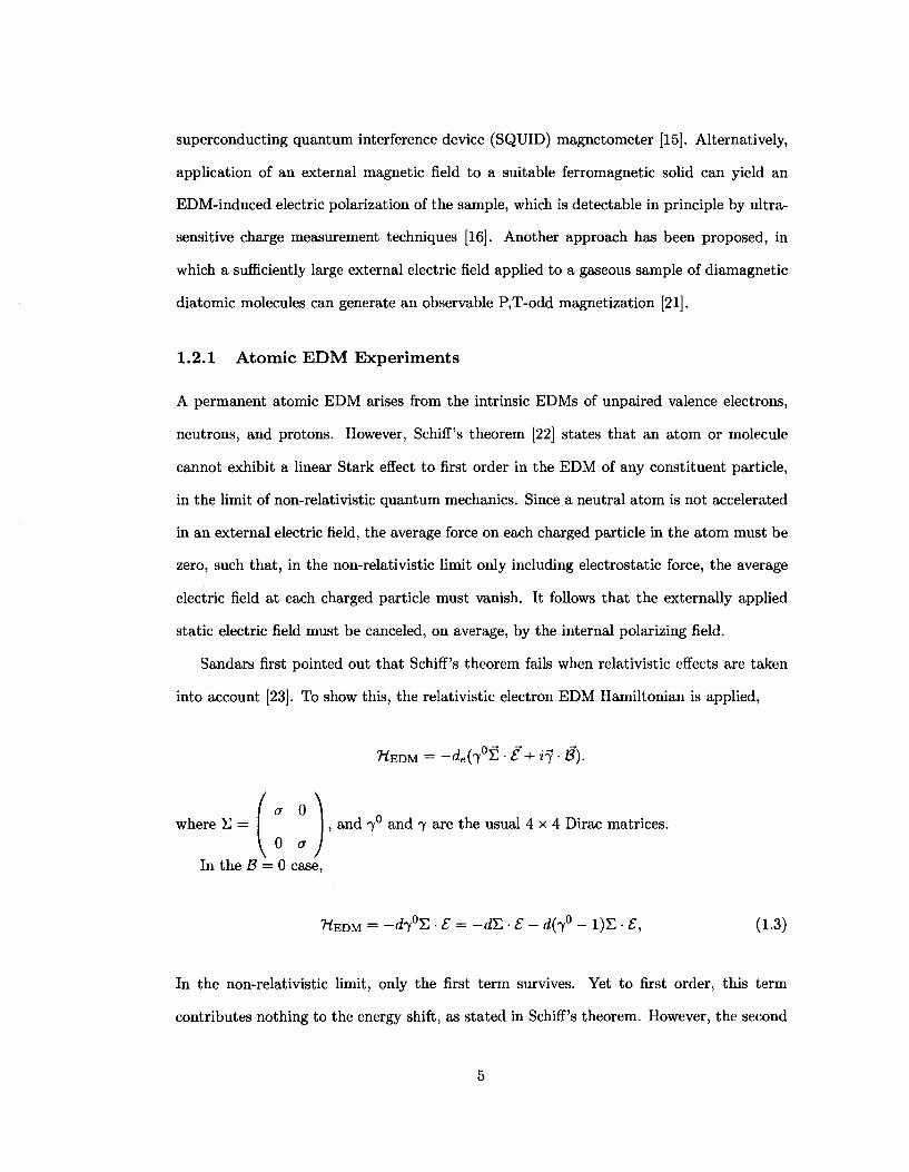
Sandars first pointed out that Schiff's theorem fails when relativistic effects are taken
into account [23]. To show this, the relativistic electron EDM Hamiltonian is applied,
»\ „ , and 7 and 7 are the usual 4 x 4 Dirac matrices.
°) case,
WEDM = -rf7°S • € = -dZ • £ - d{j° - 1)E • S, (1.3)
In the non-relativistic limit, only the first term survives. Yet to first order, this term
contributes nothing to the energy shift, as stated in Schiff's theorem. However, the second
where £ =
v° In the B = 0
5
term gives rise to the linear Stark effect associated with the EDM as the relativistic effect.
Detailed deduction leading to this effect is omitted here (Readers refer to Ref [24]). The
breakdown of Schiff's theorem here is due to the Lorentz contraction of the EDM. The
linear Stark effect due to an EDM can exist even when the expectation value of the total
electric field is actually zero, < £ > = 0. This statement is rather counter-intuitive, and
contradicts to the widespread intuitive explanation for the failure of Schiff's theorem which
assumed that the presence of relativistic effects upset the condition < £ >= 0.
The effects of P,T-violation increase in atoms with:
(i) close levels of opposite parity. The odd parity of £ in the EDM Hamiltonian HEDM
(see Eq. 1.1) requires the mixing of states with different parities. The atomic wave function
of an valence electron \ip) in the presence of an external electric field £ext to the first-order
is given as:
where EQ — En is the energy difference between close levels of opposite parity, and |i/>o)>
(IV'n)} are unperturbed atomic wave functions. The smallness of this energy difference will
increase the portion of opposite parity mixing, thus enhancing the atomic dipole moment
greatly.
(ii) a high nuclear charge Z. The enhancement factor of the effective electric field £es
experienced by de over £ext is usually denned as R = £eff/£ext = da/de, where da is the
atomic dipole moment. The linear Stark energy shift AE due to the EDM de can be written
as AE = de • £eff. The size of the enhancement factor R is determined by the relativistic
effects, the details of atomic structure, and the corresponding degree of polarization P of
the atom by the external field. R is proportional to the matrix element (V ;|^EDM|V ;)» which
receives a dominant contribution from (70 — 1) of order Z2a2 around the region very close
to the nucleus where £ ~ Ze/r2. Hence, R grows rapidly with Z as R oc Z3 approximately.
For thallium (Z=81), i?=-585 [25], and £eff is significantly enhanced over £ext.
The linear Stark shift is measured by observing the change in frequency when the
6
electric field is reversed with respect to the magnetic field. To date, measurement of
permanent EDMs in neutrons, atoms, and molecules only provide null results. The most
precise measurement of an atomic EDM in a paramagnetic system has been obtained for
205T1, giving the current limit on de [6].
1.2.2 EDM Enhancement in Diatomic Molecules
Paramagnetic polar diatomic molecules are attractive for use in the search for an electron
EDM. The strategy is to polarize the molecules along an external electric field, thereby
aligning the enormous intra-molecular field, leading to an effective enhancement of the
external field by several orders of magnitude compared to the case using atoms. This
enhancement is due to the presence of close spin-rotational levels of opposite parity.
As shown in previous section, the EDM sensitivity in the atoms is enhanced by close
levels of opposite parity and a high nuclear charge Z. Polar diatomic molecules containing
a heavy nucleus are chosen in EDM experiments, such as YbF in the ground 2£i/2 state
[26], or PbO in the metastable a(l) 3 £ i state [20]. The approximate relation for the
enhancement factor R oc Z3 also applies for the polar diatomic paramagnetic molecules
with unpaired valence electrons (see Section 1.2.1). However, nearly complete polarization
P « 1 for the polar diatomic molecules can be achieved with only a modest applied electric
field. Hence, the intrinsic sensitivity of heavy polar molecules to an eEDM can be 100~1000
times greater than for atoms.
In a polar diatomic molecule, adjacent spin-rotational states, usually separated by some
small fi-doublet splittings, or at most by energies at the order of the rotational constant
Br, are ideal candidates for the close levels of opposite parity. In the rest frame of the
diatomic molecule, the molecule possesses the axial symmetry and the electron state can be
characterized by the projection fi of electrons' total angular momentum j on the molecular
axis n (if the spin-orbit interaction is quite large). If ignoring the rotation of molecule, the
molecular energy does not change upon reflection of the molecular wavefunction in a plane
passing through the internuclear axis n, while the sign of H = j • n reverses. This indicates
7
that the states |fl > and | — Q > are degenerate, and states of definite parity constructed
as linear combinations of \Q > and | — Q > are naturally degenerate also. However, the
interaction of the electrons with the rotation of the molecule can lift the degeneracy of the
opposite parity levels. The rotational energy of the nuclei is
Hrot = BN2, N = J - j ,
where N, J , and j are the molecular rotational angular momentum, total angular momen
tum, and electron spin, respectively. The effective spin-rotational interaction is
^spin-rot = —2BJ • j .
This gives rise to the fi-doublet splitting of levels of opposite parity for the same \Q\ at
the magnitude AE ~ BJ ~ jjJRy (m and M are the mass of the electron and the
molecule respectively), which is typically 103 ~ 104 times smaller than the normal atomic
energy interval E ~ Ry, where Ry is Rydberg constant. Hence, relatively modest external
fields (« 102 ~ 104 V/cm) can cause nearly complete polarization of n along £ext. The
application of the external electric field is necessary, because otherwise, the internuclear
axis n will just precess about the molecular angular momentum J, leaving the internal
electric field £i„t oriented randomly in space, causing no net molecular EDM.
The contribution of de is included by adding the following effective EDM Hamiltonian
H ' t o VJjpin-rot:
H' = Wddej • h.
Here, Wd = j ^ i (^ I-^EDMI ^) where \l/ is the relativistic molecular electronic wave function
and //EDM = 2de ( 7 - 1 term in Eq. 1.3). The effective molecular field \ 0 a• 4 t J
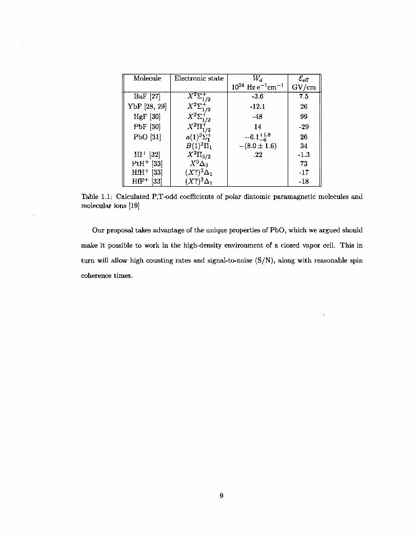
is defined as £,& = W^il. Certain paramagnetic polar diatomic molecules, listed in Table
1.1, have been identified as attractive candidates for experimental electron EDM searches.
8
Molecule
BaF [27] YbF [28, 29]
HgF [30] PbF [30]
PbO [31]
HI+ [32] PtH+ [33] HfH+ [33] HfF+ [33]
Electronic state
X S l / 2 X 2 E + 2
Y2Y+
x 2 n+ 2 a(l)3£+ £(i)3n! x 2n 3 / 2 X 3A 3
(X?)3Ai (*?)3AX
wd 1024 Hz e^cm" 1
-3.6 -12.1
-48 14
-6.1U-8
-(8.0 ±1.6) .22
£eff GV/cm
7.5 26 99 -29 26 34
-1.3 73 -17 -18
Table 1.1: Calculated P,T-odd coefficients of polar diatomic paramagnetic molecules and molecular ions [19]
Our proposal takes advantage of the unique properties of PbO, which we argued should
make it possible to work in the high-density environment of a closed vapor cell. This in
turn will allow high counting rates and signal-to-noise (S/N), along with reasonable spin
coherence times.
9
Chapter 2
Probing the Electron EDM using
PbO
In this chapter, I will describe the principles of the EDM experiment carried out at Yale.
We populate and detect fluorescence from the metastable excited state a(l) [3S+] of 208PbO
to search for an electron EDM. The principal properties of the a(l) state will be described
in Section 2.1. The experimental method and setup will be described in Section 2.2 and 2.3.
Quantum beat spectroscopy used to extract minute frequency change and the associated
data analysis methods will be discussed in Section 2.4. Statistical sensitivity and systematic
errors of the PbO experiment will be discussed in Section 2.5 and 2.6.
2.1 Principal Properties of the PbO a(l) State
Lead monoxide, PbO, is thermodynamically stable, and it is easy to obtain an isotopically
pure sample in fair amounts for research purposes at relatively low cost. The metastable
excited electronic state a(l) [3^f] has the electron configuration O\O\K\-K<I [34, 35] with
o\ and 7Ti centered on O, and oi predominantly of the Pb 6s-type. Spin-orbit interaction
mixes the nominal configuration a\a\^\i^i with configurations a\a2T^\ and a^a^X^l-,
which contain an unpaired a orbital. The unpaired electron in the molecular orbital of
10
a symmetry has no orbital angular momentum about the molecular axis. Thus it can
penetrate close to the nucleus of heavy atom Pb, yielding a significant EDM enhancement
factor [35]. This makes PbO a great candidate for eEDM experiment. The a(l) v' — 5
state can be accessed via laser excitation with laser wavelength 570 nm from the ground
electronic state X(0) ^Eg"] v ~ * vibrational level, or 548 nm from v" = 0 level, without
resort to high temperature chemistry. This wavelength range is within the range of a
tunable dye laser using rhodamine 6G (Rh6G). The a(l) state has a relatively long natural
lifetime r[a(l)] = 82(2) /xs [20]. Thus PbO can be used in a vapor cell at quite a high
density, generating very large signals. Another appealing characteristic of a(l) 3£+ state
is the existence of a very small parity-doublet splitting due to spin-rotation coupling, as
mentioned in the previous chapter. The PbO molecules can be completely polarized with
small external fields (> 15 V/cm). Even this small polarizing field yields the effective
internal electric field £eff > 107 V/cm. All the above properties make the a(l) 3Sjl~ state
of PbO a very good candidate for an EDM search1.
The a(l) state can be categorized in molecular spectroscopy as Hund's case (c)[36].
The i'th molecular electron total angular momentum jj is formed from its coupled orbital
and spin angular momenta, lj and s» respectively. The j ^ couple together to form the total
electronic angular momentum J e . In a diatomic molecule, the internuclear axis n is an
axis of rotational symmetry. J e precesses about n, forming the projection ft on the axis
n. A state with Je = 1 can have projections ft along or against the internuclear axis n:
Q = J e • n = ±1 or 0. ft couples with the rotational angular momentum N to form the
total molecular angular momentum J. Possible values of J are |fi|, |Q| + 1, \ft\ + 2, . . . In
the case of the a(l) state, the states of interest have \fl\ = 1 [36] and J = l o r 2 . J = l states
are the eEDM state and J=2 states are involved as intermediate states for laser-microwave
double resonance to populate J = l states. Two states with fl = ±1 and all other quantum
numbers identical are degenerate in the lowest approximation due to rotational symmetry xThe B(l)[3rii] (ff?ff2TiT2) state has also been considered as an EDM candidate, and the enhancement
factor is shown in Tab. 1.1, but it has a much shorter lifetime than a(l).
11
argument. However, Coriolis coupling of the electron spin to rotational motion breaks this
degeneracy, and causes a splitting ("H-doublet splitting") into two states of opposite parity,
called e and / [37], with parity (—1)J and ( - 1 ) J + 1 respectively. These are separated by
the fairly small interval ASJ(J) = qJ(J+1), where q=5.6(l) MHz is the field-free fl-doublet
splitting for the a(l) (v' = 5) [38, 39].
We can denote a(l) [3S+] using the semi-empirical description of molecular states
in the basis |7, J, M, H), where 7 denotes all the quantum numbers except for angular
momenta, as a(l) states are of Hund's case (c), and 7, J, M, fi are of complete set
of good quantum numbers. The parity of I7, J, M, Q) is characterized by the property
<7„|7, J, M, fi) = (—l)*7-51^, J,M, — fi) [40], where GV is the symmetry operator reflecting
through a plane passing through the internuclear axis. Without the perturbation from the
external electromagnetic fields, e and / components are represented in the basis |7, J, M, il),
\%J,M,e,\n\ = 1) = (|7, J,M,n = 1) - \-y,J,M,Q = - 1 » / V 2 ; (2.1)
h,j,Mj,\n\ = 1) = (|7) J,M,n = 1) + 1 7 ) J ,M,n = - i ) ) / A
with parity ( -1 ) J and (-1) , / + 1 respectively.
Using the Wigner-Eckart theorem, we can transform any operator's matrix elements
between the lab frame and molecule-fixed frame. Such a transformation is necessary be
cause many useful operators are defined in the frame co-rotating with the molecule. The
relevant transformations are
(7 ,J ,M,f i |Tf) |7 ,J ' ,M' ,n ' ) = ( - i ) J - M | J J I <7,J,n| |T( f c>||7 ' , j ' ,n'), -M q M'
(2.2)
and
(7,J ,n | |T( f e) | |7 , ,J ' ,n /)= E ( - i ) J - s V ( 2 J / + i)(2J + i) 9=-fc I - f i q Q' j
(7,0|Tf)|7',n'>.
(2.3)
12
For example, the matrix element of electric dipole moment n{^ to connect e and /
components is denned as (7, J, M, e|/xe>a|7, J, M, / ) . Since fie is defined in molecule-fixed
frame, we need to apply Eq. 2.1, 2.2, 2.3 to evaluate \xe. Because /ie is a vector operator with
rank k = 1, only terms with |Afi| < 1 will survive for (7,Sl|/i.e|'y/,0'). For the a(l) state,
|fi| = 1, hence only Q = Q' = ±1 contribute. Omitting the redundant yet straight-forward
derivation, we can have
^ = (7,J,M,e|/xe>2 |7,J,M,/>
= i ( 7 > J,M,Q = i | ^ | 7 , j,M,n' = 1) - i< 7 , j,M,n = -i\^z\^j,M,n' = -i>
x ((7,n = i|/ie|V,n = 1) + <7,n = -ll^lY.n = - i »
J ( J + 1)'
(2.4)
where / j a = (7, ft = l | /J e |y,n = 1) = (7,Q = - l | ^ e | y , f i = -1) = 1.64(3) MHzV_1cm is
the molecular electric dipole moment in the a(l) state [41].
Similarly, we can calculate the matrix elements of well as \TB • B, in the lab-
frame basis 17, J, M, Q), where /ie and n are electric dipole operator and magnetic dipole
operator respectively. They are all of the form U • V.
(7 , J ,M,n | [ / - l / | 7 , J ' ,M ' ,n ' )
+1 = {y,J,M,il\ £ (-iyUpV.p\'V,J'iM',n!)
P = - i
= (-l)2J-M~lly/(2J + 1)(2J' + l )x
^ ( J 1 J ' \
P = - I \ -M p M' ,
+1
£ 9 = - l
J 1 J'N
. -f t g fi' (7,n|y, |y,Ji '>.
13
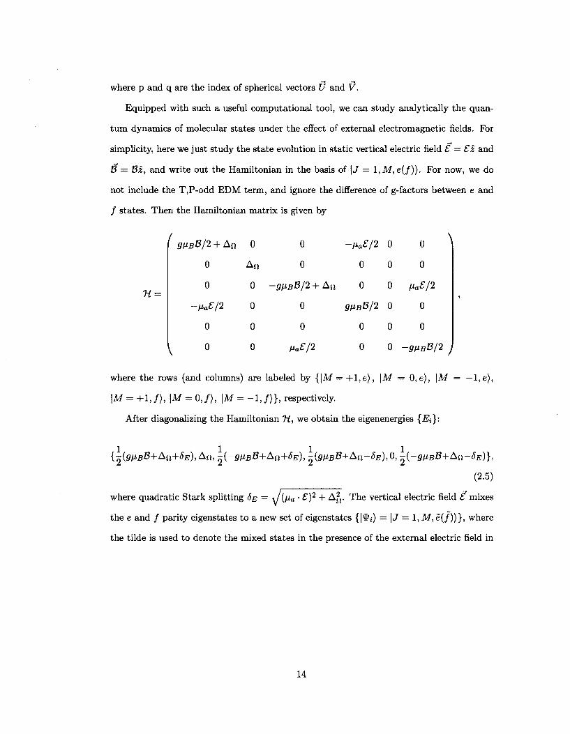
where p and q are the index of spherical vectors U and V.
Equipped with such a useful computational tool, we can study analytically the quan
tum dynamics of molecular states under the effect of external electromagnetic fields. For
simplicity, here we just study the state evolution in static vertical electric field £ — £z and
B = Bz, and write out the Hamiltonian in the basis of \J = 1,M, e(/)). For now, we do
not include the T,P-odd EDM term, and ignore the difference of g-factors between e and
/ states. Then the Hamiltonian matrix is given by
/
H =
gixBB/2 + An 0
V
0
0
-Ma£/2
0
0
A»
0
0
0
0
0 -Ma£/2 0 0
0 0 0 0
-gHBB/2 + kn 0 0 HaS/2
0 gfiBB/2 0 0
0 0 0 0
\
Ma£/2 0 0 -9HBB/2 J
where the rows (and columns) are labeled by {|M = + l , e ) , \M — 0, e), \M = —l,e),
\M = +1 , / ) , \M = 0 , / ) , \M = - 1 , / ) } , respectively.
After diagonalizing the Hamiltonian Ti., we obtain the eigenenergies {Ei}:
1 1 1 1 {^^BB+AH+SE), An, ^{-g^BB+An+SE), ^{gnBB+Au-6E), 0, -{-9HBB+&II-5E)},
(2.5)
where quadratic Stark splitting 8B — \l{^a • £)2 + A u . The vertical electric field £ mixes
the e and / parity eigenstates to a new set of eigenstates {|*j) = | J = 1, M, e(/))}, where
the tilde is used to denote the mixed states in the presence of the external electric field in
14
this literature. For example,
\J = 1 M = 1 e) = {Ail + ^ ) | J =l\M= *'e> ~ ( ^ • £ ) l J = 1.M = 1,/) ^/(An + ^ P + C/Xa^)2
" • • ^ A n - | J = l ,M = l , n = -l>;
.7 1 ^ i ~\ (An + 6E)\J = 1,M = - l , e ) + (Ma • £)j J = 1, M = - 1 , / ) ( 2 ' 6 )
\J = 1,M — — l ,e) = , „ V(A n + ^ ) 2 + (Ma-^)2
The asymptotic convergence of the M ^ 0 energy eigenstates to the molecular states
with definite fi quantum number is the result of molecular polarization in the presence of
external electric field. We can use the molecular polarization P, the ratio of Rabi frequency
fj,a£ over the Stark splitting 5E, as a measure of the Stark mixing of e and / states.
P= . >*a£ = . (2.7) y/iva-sy + Ah
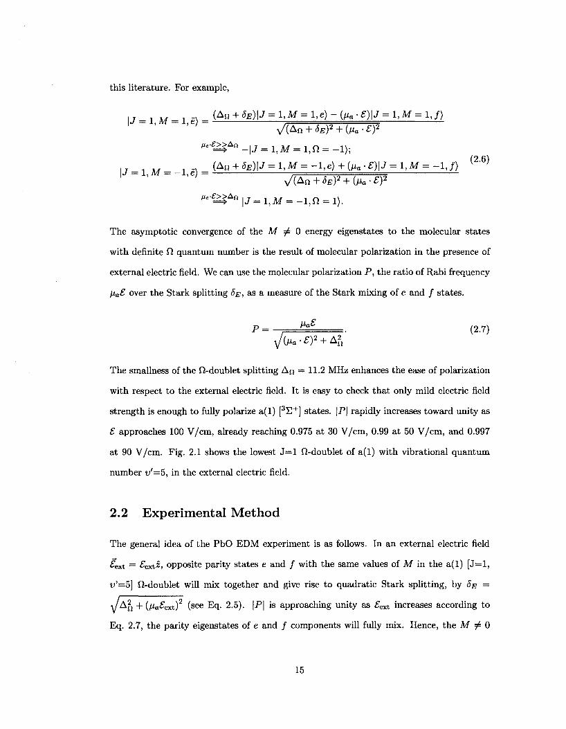
The smallness of the fi-doublet splitting An = 11.2 MHz enhances the ease of polarization
with respect to the external electric field. It is easy to check that only mild electric field
strength is enough to fully polarize a(l) [3S+] states. \P\ rapidly increases toward unity as
€ approaches 100 V/cm, already reaching 0.975 at 30 V/cm, 0.99 at 50 V/cm, and 0.997
at 90 V/cm. Fig. 2.1 shows the lowest J = l fi-doublet of a(l) with vibrational quantum
number v'=b, in the external electric field.
2.2 Experimental Method
The general idea of the PbO EDM experiment is as follows. In an external electric field
£ext = £ext£, opposite parity states e and / with the same values of M in the a(l) [J=l,
D ' = 5 ] H-doublet will mix together and give rise to quadratic Stark splitting, by 5E =
JA2j + (/J.a£ext) (see Eq. 2.5). \P\ is approaching unity as £ext increases according to
Eq. 2.7, the parity eigenstates of e and / components will fully mix. Hence, the M ^ 0
15
N X
c«
90
60
30 A 00 c '£ * - H
o. c« -^
t-H C3
0-
-30-
-60 A
-90-
Voltage across Cell (V) 76 152 229 305 381
E Field (V/cm)
Figure 2.1: a(l) [3£^] ft-Doublet in the Electric Field. The dash line shows the polarization reaches 0.975 at 30 V/cm, 0.986 at 40 V/cm, and 0.99 at 50 V/cm. The energy level diagram shows the Stark splitting at 40 V/cm with 152 V across the electrodes with 1.5" spacing.
16
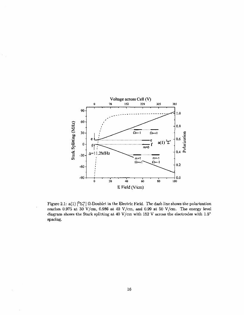
energy eigenstates correspond to definite fi rather than definite parity. The energy of the
molecule can be written as
BrJ(J + 1) + Wdden - /j,e£ext^M/J(J + 1), (2.8)
where Br is the rotational constant and Wd — fi£eff is the EDM enhancement factor for the
PbO a(l) state [35]. The semi-empirical estimate of Ref. [35] is \Wd\ > 1.2x 1025 Hz/(e-cm).
A separate theoretical effort using a configuration interaction calculation concludes Wd =
-(6.1+J;|) x 1024 Hz/(e • cm) [31], agreeing within a factor of 2. As the a(l) 3E+ state
of PbO is the excited states with two unpaired valence electrons, it is difficult to do the
electronic structure calculations on such a molecular system, so the discrepancy within
a factor of 2 is acceptable and further theoretical investigation will be motivated by the
progress of experiment.
i 8B > .
8E
Sd
*
de=0 &#) B
Figure 2.2: Schematic Diagram of Energy Levels of a(l) 3S+ PbO. The shifts in M=±l levels of the upper and lower fi-doublet components of the a(l)[J=l, v'=5] state of PbO in the external fields. In left panel, dotted lines: level positions in the absence of external magnetic field and assuming de=0; solid lines: Zeeman shifts in presence of Bz ^ 0 but de = 0 still assumed. In right panel, additional shift in solid lines, Bz ^ 0 and de ^ 0 assumed.
Hence, there is an additional contribution Sd in the situation de ^ 0, Sd = de£ef[ with
£eff = Wd$l, different sign for the Q, = 1 and D, — — 1 components of the J7-doublet in the
17
polarized state. Such a difference in sign is very significant because it provides an excellent
opportunity for effective diagnostics and suppression of systematic errors. We will discuss
this point further in Section 2.6.3.
To detect this shift Sj in the EDM search, we apply a static magnetic field B — Bz
which shifts the a(l) levels further by gpfj,BBM/J(J + 1), where \IB is the Bohr magneton,
and gp is the effective g-factor of the polarized state taking into account of g-factor intrinsic
difference from different fi-doublet components Sg = ge~gf and perturbed difference due to
the Stark mixing of J=2 rotational level (such effect will be discussed later in Section 2.6.1
and Section 5.2). ge(9f) is the Lande g-factor in the molecule-fixed frame of the e(/)
member of the fi-doublet and gp « 1.86 for the a(l) state. The coherent state precesses
around the external field direction z and accumulates the relative phase between the M=±l
components with time due to the different Zeeman 5B and EDM shifts Sd- The effects of
applied electric and magnetic fields on the a(l) J= l , v'—b fi-doublet is summarized in
Fig. 2.2.
The spontaneous decay from the a(l) (v'=5) to X(0) (v"=0) has a Franck-Condon
factor as large as 50% and emits the fluorescence at 548nm. The Franck-Condon factor
between a(l) (i/=5) and X(0) {v"=l) is also ~50%, but due to the technical difficulty in
suppressing scattered laser light and induced transient in detectors, the wavelength range
of detection is chosen to differ from the excitation. The coherent interference between
M — 1 and M = - 1 Zeeman sub-levels yields quantum beats in fluorescence signal with
beat frequency 2{gPnsB ± de£eft)/h, including the EDM contribution, where the sign is
determined by the relative alignment between magnetic field and internal effective electric
field. We detect this precession as Zeeman quantum beats, which modulate the exponential
decay in the unpolarized fluorescence intensity at the beat frequency.
The EDM effect can be distinguished by the dependence of the beat frequency on the
relative alignment of £ and B and the choice of fi-doublet pair. Since populating the
different fi-doublet components is equivalent to flipping the internal electric field with the
external electromagnetic field configuration left intact, this additional degree of freedom
18
provides the appealing co-magnetometer mechanism to suppress systematic effects.
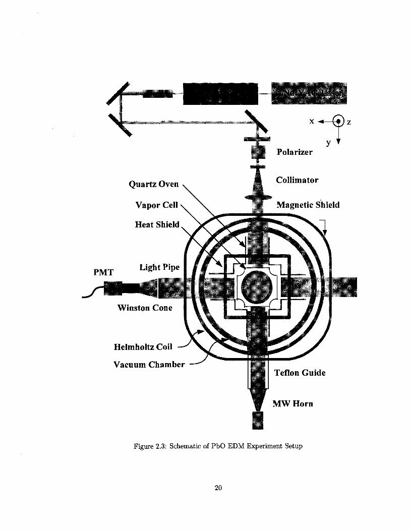
2.3 Experimental Setup
The PbO EDM experiment at Yale is carried out in a vapor cell containing PbO at the
operating temperature 700°C, shown in Fig. 2.3. A barrier to molecule-based searches for
de has been the production of suitable molecules and the effective detection at high counting
rates. The natural lifetime of the PbO a(l) state T [a(l)] = 82(2) fis [20] is too short to be
useful in a beam experiment. Other candidates potentially suitable to beam experiment
will be discussed later in Section 6.3. At the time of the startup of our experiment, there
were no mature methods to produce cold molecule beams with high density. The vapor
density of PbO in the vapor cell can be substantially high, so our experiment adopts the
cell scheme to measure the electron EDM.
The vapor cell for PbO consists of an hollow alumina frame with top and bottom end
caps supporting flat gold foil electrodes 6 cm in diameter, surrounding guard ring electrodes
used to improve electric field homogeneity, and large flat sapphire windows on all four sides
that are sealed to the frame with gold foil as a bonding agent. The electric field £ext = Sextz
is quite uniform over a cylindrical volume of diameter 5 cm and height 3.8 cm, and is chosen
in the range 30~100 V/cm. The cell is enclosed in an quartz oven which sits inside opaque
quartz heat shields in a vacuum chamber. One pair of Helmholtz coils carries DC current
to control the vertical magnetic field Bz in the range 50~200 mG. Four sets of mutually
perpendicular coils made of cosine-distributed rods, two in Helmholtz configuration, two in
anti-Helmholtz configuration, generate the homogeneous magnetic fields and the gradient
fields along x and y, respectively, providing systematic diagnostics on magnetic fields. The
chamber and magnetic foils are enclosed by up to four layers of magnetic shields to screen
out the spurious magnetic field.
The relevant EDM states for the experiment are the a(l) (t/=5) 3 E + J= l , M=±l
levels of either the upper or lower a(l) fi-doublet. The state preparation to populate the
19
Polarizer
PMT
Quartz Oven
Vapor Cell
Heat Shield
H Collimator
Magnetic Shield
Light Pipe
$ •"• • v .5 1 | | i ^ ^ H
"' -. 'Ac • til illillllljl
Winston Cone
Helmholtz Coil
Vacuum Chamber Teflon Guide
MW Horn
Figure 2.3: Schematic of PbO EDM Experiment Setup
20
coherent superposition of states of interest is via laser-microwave double resonance. We
populate the J = l M=0 state of PbO by laser excitation from the ground electronic state
X(0) (v = 1) and microwave population transfer to J= l , M = ±1 states is accomplished
via an intermediate state (the a(l) J=2 state).
A pulsed laser beam with vertical z linear polarization and wavelength ~571nm prop
agates along y direction and excites the following transition:
X[J = 0+,v = 1] -> o(l) [J = 1~,M = 0,t/ = 5] .
The dye laser used here is pumped by the second harmonic of a Nd:YAG (yttrium alu
minum garnet) laser at a repetition rate of 100 Hz and delivers 10~20 mJ/pulse of light
at wavelength ~571 nm propagating in the y direction to the vapor cell. The pulses are 8
ns long with a line width of ~1 GHz, comparable to the Doppler width of the transition.
The laser light traverses the vacuum chamber and oven in a 5 cm diameter light pipe to
the cell, then exits through another light pipe.
Following the laser pulse, a Raman transition is driven by two microwave beams prop
agating in the -y direction. The first, with z linear polarization, excites the upward 28.2
GHz transition:
a(l)[J = I", Af = 0,t/ = 5] - • a(l) [J = 2+,M = 0,t/ = 5] .
The second, with x linear polarization and detuned to the red or blue with respect to the
first by 20~70 MHz, drives the downward transition:
o(l)[J = 2+,M = 0,v' = 5] -+ a(l) [J = 1,M = ±l,v' = 5] .
As the result, nearly 50% of the J= l~ M=0 molecules are transferred to a coherent super
position of M = ±1 levels in the desired fi-doublet component. The fluorescence from the
21
decay:
a(l)[J = 1, Af = ± l , t / = 5] -» X(0) [t>" = 0] ,
is captured by a light pipe along the x direction and orthogonal to the laser beam. The
fluorescence passes through an infrared-blocking filter and one interference filter, which
blocks scattered laser light and most blackbody radiation from the ovens while passing
the signal of interest to a photomultiplier tube (PMT). The quantum beat frequency is
extracted from the Fourier transform and least square fitting of the data.
2.4 Quantum Beat Spectroscopy in Fluorescence
The essential part of the PbO EDM experiment is to detect minute changes 8v in the
spin precession frequency of the PbO molecules. This change should be correlated with
the relative orientation of the applied electric field £ with respect to the applied magnetic
field B. In addition, the f2-doublet structure of PbO means that 5u should reverse as the
internal electric field changes orientation with respect to the magnetic field via $7-doublet
reversal; this can be accomplished through microwave selective excitation without changing
external electric or magnetic fields. The details will be discussed in Chapter 4.
Quantum-beat spectroscopy [42, 43] provides a robust way to extract the spin precession
frequency v\, precisely and accurately, by measuring the modulated intensity due to coherent
interference between fluorescent decay channels. This signal is almost immune to Doppler
effects and pulse to pulse laser power fluctuations. The states in coherent interference will
experience the same Doppler shift and hence cancel out the Doppler effect by beating at
the frequency difference between them.
Here I will give a brief overview on the quantum beat spectroscopy with its application
to the a(l) [3S+] state of PbO, and the data analysis process to interpret the quantum
beat signal.
22
2.4.1 Quantum Beats
After we populate the excited levels a(l) J = l v' = 5 at time t = 0, each component of
the excited state represented in the energy eigenbasis (I'i'i)} will evolve at the frequencies
corresponding to its energy {E{} derived in Eq. 2.5. Hence at later times t, the wavefunction
can be written as |*e(*)) = Ylie~iEit\^i)(^i\^e(0)), where *e(0) is the initial excited
state. The a(l) J = l state can spontaneously decay down to various sub-levels of the
ground state X(0), with the selection rules AJ = 0, ±1 and a change in parity for this El
transition. The fluorescence intensity will be sinusoidally modulated due to interference
between the Zeeman sub-levels in a(l) states in each decay channel. In quantum mechanics,
it is assumed that there are no coherent interferences between multiple final states [44],
therefore we just sum over all possible final states with different Jf and Mf, incoherently.
Then the total fluorescence intensity I satisfies
Jf Mf
Jf Mf
Y,(Jf,Mf,n = 0\r.e\Ve(t)) Me
(2-9)
Y, £ e - " * « ( J / , Mf, n = 0|f• c|tti><*i|*e(0)> , Me i
where e is the light polarization detected and Me^ is the magnetic quantum number of the
initial(final) state. Due to the breaking of the degeneracy of each level and the resulting
state precession at frequencies corresponding to the energy differences, the fluorescence
intensity oscillates with time. This oscillation is detectable within few MHz bandwidth
as the Zeeman splitting of J = l level (100 ~ 400 KHz under our nominal experimental
condition).
After the arrival of the pump laser pulse, the molecules will be excited to some su
perposition of the M sub-levels of the J = l state. For example, suppose |*&e(0)) = {\M =
l,e) + e%<^\M = —l,e))/>/2. This can be prepared by the direct excitation from the X(0)
J=0 ground state by a horizontally polarized laser pulse tuned to the R0 line (in the absence
of the external electric field). Due to the energy splitting between these sub-levels, the ex-
23
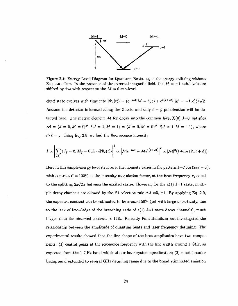
M=l M=0 M=-l
Figure 2.4: Energy Level Diagram for Quantum Beats. u>o is the energy splitting without Zeeman effect. In the presence of the external magnetic field, the M = ±1 sub-levels are shifted by ±w with respect to the M = 0 sub-level.
cited state evolves with time into |*e(*)) = (e - i w ' |M = l,e)+ ei^+wt^\M = -l,e))/\/2.
Assume the detector is located along the x axis, and only i = y polarization will be de
tected here. The matrix element M for decay into the common level X(0) J=0, satisfies
M = {J = 0,M = 0\f-i\J = \,M = 1) = (J = 0,M = 0|f • t\J = 1,M = -1) , where
r-e = y. Using Eq. 2.9, we find the fluorescence intensity
Joe Me
oc Me~iwt + Mei{,t>+Ult) oc |.M|2(l+cos(2u;i+ <£)).
Here in this simple energy level structure, the intensity varies in the pattern 1+C cos (2ut + </)),
with contrast C — 100% as the intensity modulation factor, at the beat frequency Uf, equal
to the splitting 2UJ/2~K between the excited states. However, for the a(l) J = l state, multi
ple decay channels are allowed by the El selection rule A J =0, ±1 . By applying Eq. 2.9,
the expected contrast can be estimated to be around 50% (yet with large uncertainty, due
to the lack of knowledge of the branching ratio of a(l) J = l state decay channels), much
bigger than the observed contrast « 12%. Recently Paul Hamilton has investigated the
relationship between the amplitude of quantum beats and laser frequency detuning. The
experimental results showed that the line shape of the beat amplitudes have two compo
nents: (1) central peaks at the resonance frequency with the line width around 1 GHz, as
expected from the 1 GHz band width of our laser system specification; (2) much broader
background extended to several GHz detuning range due to the broad stimulated emission
24
from the dye laser. This beat amplitude spectrum, convolved with the rotational spec
trum of the PbO a(l) state, will introduce the intervention of the adjacent rotational lines
(names R6, R5 and Rl) to contribute the background which will diminish the contrast of
quantum beats. Quantatitively the smallness of the observed contast appears consistent
with measured laser spectrum and the overlap with these rotational lines.
By extracting the minute changes Aui, in the spin precession frequency of the PbO
molecules versus relative orientations of the applied electric field £, applied magnetic field
B, and the internal electric field determined by MU (see Eq. 2.8), we can characterize
the size of the EDM signal. The contrast C is an important measure of the experimental
sensitivity [45], since the uncertainty 5v in determining v is limited by
x ^ Of ~ .
27rCTv VtoT
where r is the lifetime of quantum beat signal and JVtot is the total number of counted
photon events.
2.4.2 Data Analysis
In practice, we must include multiple parameters to explain the signal output from the
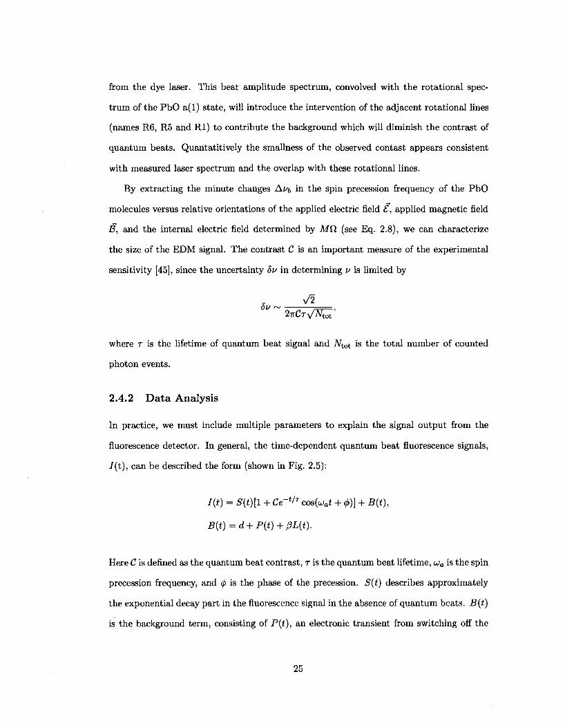
fluorescence detector. In general, the time-dependent quantum beat fluorescence signals,
7(t), can be described the form (shown in Fig. 2.5):
I(t) = S(t)[l + Ce-'/T cos(u;a* + (j>)} + B(t),
B{t) = d + P{t) + pL(t).
Here C is defined as the quantum beat contrast, r is the quantum beat lifetime, uia is the spin
precession frequency, and <j> is the phase of the precession. S(t) describes approximately
the exponential decay part in the fluorescence signal in the absence of quantum beats. B(t)
is the background term, consisting of P{t), an electronic transient from switching off the
25
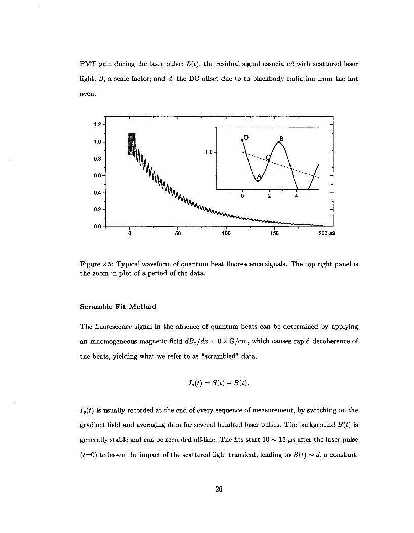
PMT gain during the laser pulse; L(t), the residual signal associated with scattered laser
light; /3, a scale factor; and d, the DC offset due to to blackbody radiation from the hot
oven.
1.2-
1.0-
0.8-
0.6-
0.4-
0.2-
0.0-I 1 . , , , 1 1 , ,
0 50 100 150 200 \iS
Figure 2.5: Typical waveform of quantum beat fluorescence signals. The top right panel is the zoom-in plot of a period of the data.
Scramble Fit Method
The fluorescence signal in the absence of quantum beats can be determined by applying
an inhomogeneous magnetic field dBz/dz ~ 0.2 G/cm, which causes rapid decoherence of
the beats, yielding what we refer to as "scrambled" data,
Is(t) = S{t) + B{t).
Ia(t) is usually recorded at the end of every sequence of measurement, by switching on the
gradient field and averaging data for several hundred laser pulses. The background B{t) is
generally stable and can be recorded off-line. The fits start 10 ~ 15 /xs after the laser pulse
(£=0) to lessen the impact of the scattered light transient, leading to B(t) ~ d, a constant.
26
The fluorescence decay envelope S(t) ss iVoexp(—t/T\), where the effective state lifetime
T\ ~ 50 fis and NQ the initial amplitude of fluorescence decay.
Fitting is carried out in two steps. The first step is to fit Ia(t) using the approximate
form
/*(*) « /*o(0 = Ae-llT + B
to extract the background constant term B and the lifetime T. However, S(t) deviates
from an exact exponential form, due to wall quenching and time-dependent acceptance
changes resulting from diffusion of the excited molecules. This makes it hard to describe
the shape of S(t) by a simple exponential decay. The constant term B affects the quality
of the approximation of the exponential decay, so it's worthwhile to fit it instead of just
averaging the end of the data sequence. We define the difference function S(t) = Is(t) — B,
and use the approximation S(t) « S(t) for further fitting.
The second step of fitting is to fit the beat fluorescence signal
I(t) = AS(t)[l + Ce~tlT cos(w„i + </>)] + B.
Initial guesses for the parameters A, uja, C, r, <j> and B are important for the success of
the fit. A ~ 1 is the scale factor to account for the laser intensity fluctuation between
data and scrambled signal. The quantum beat frequency ua = uaj2rK a 125 ~ 400 kHz,
corresponding to the magnetic field B « 50 ~ 160 mG, can be estimated with reasonable
accuracy from the power spectrum of the data using the Fast Fourier Transform (FFT). The
beat contrast C « 0.1 can be estimated using the extrema in the first period Ta = 27r/u;a,
shown in Fig. 2.5: C = (IA — IB)/IC, where the point A is the maximum, B minimum,
and C the mid-point of A and B. The beat phase <j> can be estimated from the interval
between point O and point C, and the period Ta. Finally the beat lifetime r ~ 100 /zs, in
additional to the state lifetime T, accounts for shortening of the beat coherence time by
collisions and broadening.
27
The Levenberg-Marquardt method [46] is used for the multiple-parameter fitting. It
combines the steepest descent method with Newton's method in the determination of the
minimum of x2'
where {Jj} are the time-resolved measurement of fluorescence at the sampling time {£j},
and o{Ii) is the uncertainty, or noise, associated with 7j at ij. In the shot noise limit, we
can write cr(Ii) = a^/\Ii\, where a is a proportionality factor, a is estimated from the
standard deviation of the data in last several tens of microseconds, typically from 170 /is
to 200 fis, where the quantum beat pattern has died out since the lifetime is only ~ 50 /AS
and the tail of data series is approximately equal to the background B. B is mainly from
the blackbody radiation and its statistical uncertainty is characterized by the shot noise.
Hence, a « a(B)/-l/\B~\. In the case where the noise on the background is dominant, the
noise a(I) ss cr{B) is independent of time and the statistical uncertainty on the frequency
determination is
*-s&$ni"*hfi- (2'10)
where SQ = IQ — B is the initial signal size and Bd is the bandwidth of our detection system;
Bd — 25 with, the sampling interval At; and a{B)/\/B~d is a constant independent of At,
which is determined by the experiment setup and the detection scheme. This formula can
be derived from the error matrix associated with the x2 [45].
Although this fitting method using the direct measurement of scrambled signals gives
rather satisfying results, the procedure requires a separate step to record the scrambled and
background signals. This method relies greatly on the stability of the experimental config
uration, such as ambient magnetic field, oven temperature, and laser intensity, etc, to reach
a consistent cancellation of the backgrounds. This procedure was used with no magnetic
shields in place previously. However, the application of the magnetic gradient field will
change the magnetization of the magnetic shields and perturb the nominal magnetic field
distribution as well. The degaussing process required to correct the residual magnetization
28
would severely limit the duty cycle of the data collection. So after the development of a
new data fitting method discussed in the next section, this procedure is obsolete.
Improved "Scrambled" Data Generation Method
An improved method is to use a forward and backward difference operation on the fluores
cence data to get a self-contained "scrambled" signal [47, 48], instead of taking extra time
to record scrambled data. This technique was generalized to arbitrary order corrections
and adapted to our experiment by Paul Hamilton. One quarter of the data is shifted for
ward in time by half a precession cycle, another quarter of the data is shifted backward in
time by half a precession cycle, and the one-half of the data remains untouched. The sum
gives the scrambled data:
I's(t) = [2I(t) + I(t - Ta/2) + I(t + Ta/2)} /4.
Here the period of a precession cycle is Ta = 2-n/ua. This self-contained "scrambled"
signal can be used in place of the directly-measured scrambled signal, to feed into the
fitting procedure described above.
To get a better understanding of this method, let's take a look at the scrambled data
first. The deviation of the signal decay pattern S(t) from a simple exponential function
can be explained by a geometric factor G(t), which takes into account various source
of geometry-dependent factors: the finite acceptance angle of the light pipe, the angle-
dependent transmission of the interference filter, the wall-collision de-excitation of the
excited state, and solid angle change due to the molecules diffusion in the vapor cell. Here
S(t) = G(t)exp(-t/T). We can model molecules initially randomly distributed inside the
vapor cell and diffusing with a Maxwell velocity distribution using Monte-Carlo simulation.
If the trajectory of the molecule intersects the cell walls, it is assumed that the molecule
is de-excited. Otherwise, the excited molecules will decay with the natural lifetime of the
a(l) [3S+] state. We can determine the total number of the excited molecules at any
29
given time by counting any surviving molecules. This Monte-Carlo result yields reasonable
agreement with experimental data for the observed decay pattern. In particular, it explains
clearly why the signal appears to decay with a apparent lifetime of 40 ~ 50 /xs although
the natural lifetime of the a(l) [3S+] state is known to be T « 80 fis. Further light
tracing algorithm can be applied to include the other geometric factors. Emitted rays
from molecular spontaneous emission are traced to determine if they intersect the light-
pipe aperture. If they do, the ray will be collected by the detector, with their intensity
modified by a factor proportional to the transmission of the interference filters at the angle
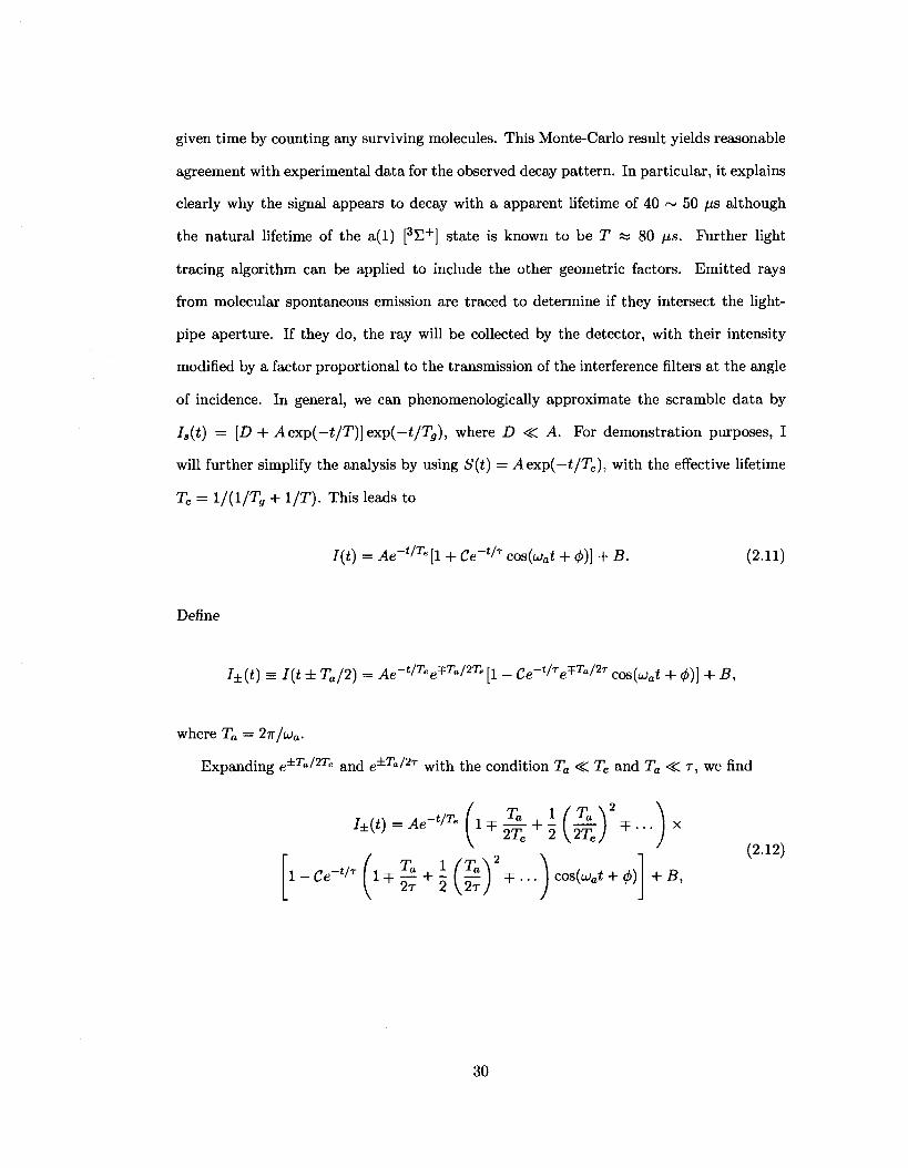
of incidence. In general, we can phenomenologically approximate the scramble data by
Is(t) = [D + Aexp(—t/T)]exp(—t/Tg), where D -C A. For demonstration purposes, I
will further simplify the analysis by using S(t) = Aexp(—t/Te), with the effective lifetime
Te = 1/(1/TS + 1/T). This leads to
I(t) = Ae~t/T° [1 + Ce~t/T cos{uat + <f>)] + B. (2.11)
Define
I±(t) = I(t ± TJ2) = Ae-^e^/^ll - Ce-t<re*T°'2r cos(u;a* + </>)] + B,
where Ta = 2n/ua-
Expanding e± T a /2 T e and e±Tal2r with the condition Ta < Te and Ta «: r , we find
W)-^-^-(l^ + i (^ )%. . . )x
l - C e - ^ ( l T | + i(|)%...)cosM + ^)
(2.12)
+ B,
30
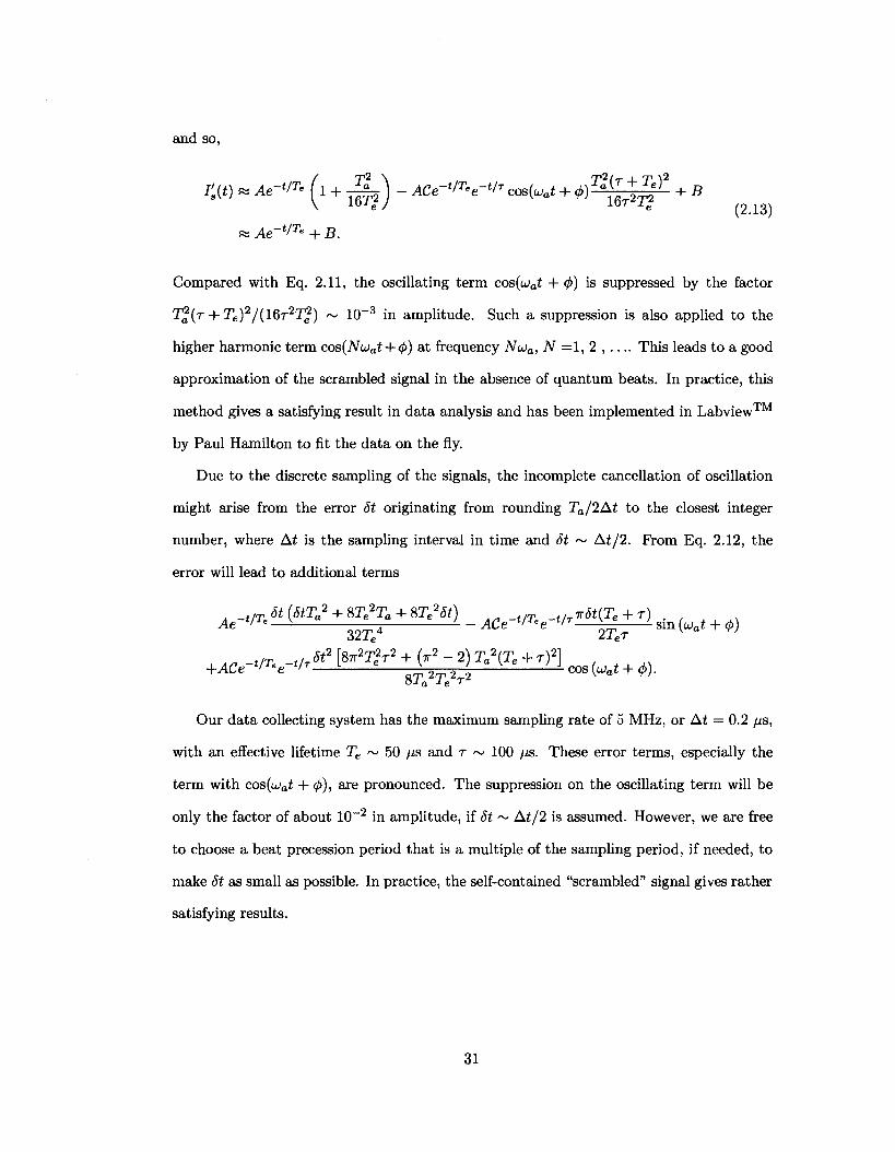
and so,
I's(t) « Ae-VT* ( l + i ^ ) " ACe-We-** cos(u>at + ^ f + B
(2.13) « Ae'1^ + B.
Compared with Eq. 2.11, the oscillating term cos{u)at + 4>) is suppressed by the factor
T 2 ( T + Te)2/(16r2T(
2) ~ 10 - 3 in amplitude. Such a suppression is also applied to the
higher harmonic term cos(Nujat + <j>) at frequency Nu>a, N =1, 2 , — This leads to a good
approximation of the scrambled signal in the absence of quantum beats. In practice, this
method gives a satisfying result in data analysis and has been implemented in Labview™
by Paul Hamilton to fit the data on the fly.
Due to the discrete sampling of the signals, the incomplete cancellation of oscillation
might arise from the error St originating from rounding Ta/2At to the closest integer
number, where At is the sampling interval in time and St ~ At/2. Prom Eq. 2.12, the
error will lead to additional terms
ft (ftT.' + «r.-r.+ «-.'*) _ ACe-t/T.e^m + r}
32Te4 2Ter
v Yi
Our data collecting system has the maximum sampling rate of 5 MHz, or At = 0.2 /JS,
with an effective lifetime Te ~ 50 /xs and T ~ 100 /is. These error terms, especially the
term with cos(ujat + (j>), are pronounced. The suppression on the oscillating term will be
only the factor of about 10~2 in amplitude, if St ~ At/2 is assumed. However, we are free
to choose a beat precession period that is a multiple of the sampling period, if needed, to
make St as small as possible. In practice, the self-contained "scrambled" signal gives rather
satisfying results.
31
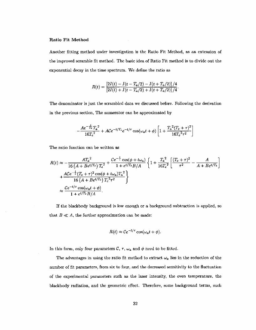
Ratio Fit Method
Another fitting method under investigation is the Ratio Fit Method, as an extension of
the improved scramble fit method. The basic idea of Ratio Fit method is to divide out the
exponential decay in the time spectrum. We define the ratio as
n(f, = [2I(t)-I(t-Ta/2)-I(t + Ta/2)}/4 " W [2/(t) + I(t - Ta/2) + I(t + Ta/2)} /4 •
The denominator is just the scrambled data we discussed before. Following the derivation
in the previous section, The numerator can be approximated by
Ae~^Ta2
im 2 + ACe-t/Tee~tlT cos(uat + cj>) 1 +
Ta2(Te + r)2
16Te2r2
The ratio function can be written as
DM ATa2 • Ce-tcaaW + tUg) f, , T2 \(Te + r)
+
16(A + Bt*/T')Te2 l + et/T'B/A \ 16Te
2 L ?2 A + Be*/7'
ACe-r(Te + r ) 2 cos(<ft + tuia)Ta2 }
16(^ + Be'/re)Te2T2 J
^ Ce~^T cos(ujat + 4>) * H-e^B/A '
If the blackbody background is low enough or a background subtraction is applied, so
that B < A , the further approximation can be made:
R{t) « Ce" t /T cos(u;a* + <j>).
In this form, only four parameters C, T, uia and <j> need to be fitted.
The advantages in using the ratio fit method to extract uja lies in the reduction of the
number of fit parameters, from six to four, and the decreased sensitivity to the fluctuation
of the experimental parameters such as the laser intensity, the oven temperature, the
blackbody radiation, and the geometric effect. Therefore, some background terms, such
32
as the scale factor A and the blackbody background B, may be neglected when fitting
the data. Such a fitting method is used in Muon g-2 experiments [47, 48] and is under
investigation for the applicability to our experiment.
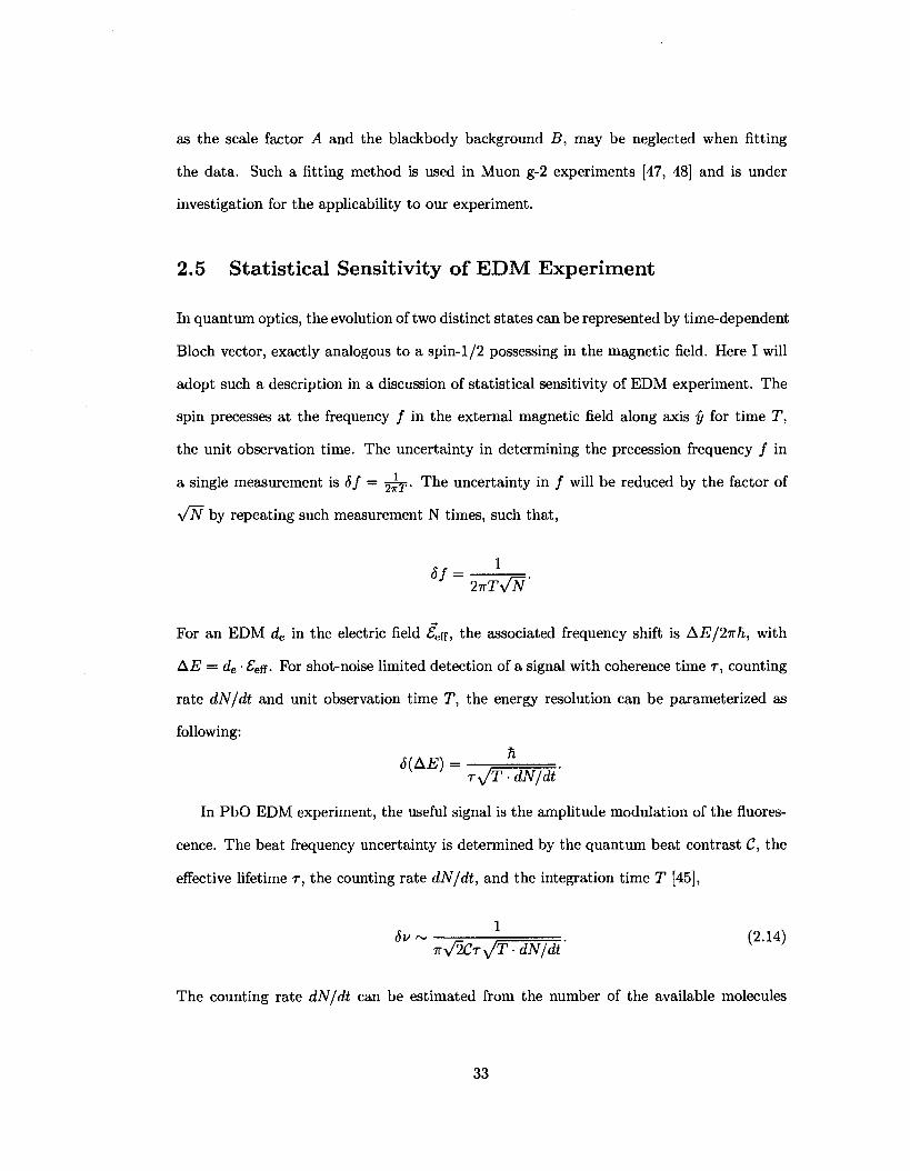
2.5 Statistical Sensitivity of EDM Experiment
In quantum optics, the evolution of two distinct states can be represented by time-dependent
Bloch vector, exactly analogous to a spin-1/2 possessing in the magnetic field. Here I will
adopt such a description in a discussion of statistical sensitivity of EDM experiment. The
spin precesses at the frequency / in the external magnetic field along axis y for time T,
the unit observation time. The uncertainty in determining the precession frequency / in
a single measurement is Sf — -^j,. The uncertainty in / will be reduced by the factor of
\/N by repeating such measurement N times, such that,
Sf = 2irTy/N'
For an EDM de in the electric field £eff, the associated frequency shift is AE/2irh, with
AE = de • £es. For shot-noise limited detection of a signal with coherence time r, counting
rate dN/dt and unit observation time T, the energy resolution can be parameterized as
following:
5(AE) = h
Ty/T-dN/dt'
In PbO EDM experiment, the useful signal is the amplitude modulation of the fluores
cence. The beat frequency uncertainty is determined by the quantum beat contrast C, the
effective lifetime r, the counting rate dN/dt, and the integration time T [45],
Sv = ] (2.14) Try/2CTy/T- dN/dt
The counting rate dN/dt can be estimated from the number of the available molecules
33
jV in the useful rovibrational level for the laser excitation to start with, the excitation
efficiency ee, detection efficiency e<2, decay branching to X(0) v" = 0 level /FC , and the
laser repetition rate r,
dN/dt ~ AfrteedfFC.
Our experiment aims at achieving improvements on the excitation efficiency, detection
efficiency, and the beat contrast to increase the sensitivity to the electron EDM. This
thesis is devoted to discuss the current progress of this experiment. The experimental
setup and preliminary experiment result will be described in Chapter 3, 4 and 5 in this
thesis. The status of this experiment with improvements on the excitation efficiency and
detection efficiency will be described in Chapter 6. Readers please refer to Section 6.1 for
the estimation of the excitation efficiency, detection efficiency, and the beat contrast.
2.6 Overview of Systematic Effects
Great concern has been taken in examining the systematic effects since EDM searches, as
precision experiments are quite susceptible to systematic effects. Due to the smallness of
the electron EDM compared to the magnetic moment, all of the EDM experiments are
especially sensitive to the spurious magnetic fields. If a change of the magnetic field B is
associated with the application of the external electric field £ and dependent on the field
strength, the frequency difference derived from the field reversal could yield a false EDM
signal which will be hard to distinguish from the authentic EDM signal. Such systematic
effects can be shown as follows. The Larmor frequency in the external fields, following the
notation in Eq. 1.1, is
#T ,£T: wTT = ft(B + a£ + f3£2) + d£,
B1,£i- <"u = M B -<*£ + P£2) - d£,
ujf — UJ^I = 2(d + jia)£.
34
Here a and /3 are the linear and quadratic coefficients of a stray magnetic field dependent
on the electric field. These stray fields are the result of imperfections that are related to
the details of the experimental apparatus, such as inhomogeneity of electric fields, inhomo-
geneity of magnetic fields, etc. To most EDM experiments, two types of systematic effects
are of special concern: transverse magnetic fields associated with the molecules' motion
in the electric field and the geometric phase, and vertical magnetic fields associated with
leakage currents. Both can generate stray 5-dependent magnetic fields. These types of
effects must be diagnosed by systematic variation of experimental configurations.
2.6.1 Applied External Field
The molecules moving in an electric field £ and magnetic field Bo will experience a magnetic
field in their rest frame Bm = v x £/c, where £ and BQ are nearly parallel with angle 6.
The motional magnetic field is prominent in the atomic beam experiment where the atoms
propagate along the definite direction perpendicular to the applied electric field and large
electric field is required to induce the polarization of atomic states. For the Berkeley Tl
EDM experiment [49], the beam velocity is v ss 3.9 x 104 cm s_1, and the applied electric
field is £ «s 107 kV/cm, so the motional magnetic field is Bo « 0.5 mG compared to
the nominal applied magnetic field 0.42 G. Two counter-propagating atomic beams were
used to cancel the systematic effect due to the motional magnetic field. In experiments
using vapor cells, the atoms or molecules are moving randomly inside the cell and have the
average < v > = 0 without any preferential direction. Imperfect excitation caused by laser
or microwave detuning and/or wavefront curvature, will cause the preferential selection of
a certain velocity class due to the Doppler effect and hence may introduce a certain level
of preferential direction.
However, in our EDM experiment using molecules, this systematic effect is highly sup
pressed, because the close-lying parity states in molecules will induce a large Stark tensor
effect. This suppresses the level shift due to the transverse magnetic field, as shown in
the following discussion. Under the typical experimental condition where the electric field
35
is strong enough that the molecules are almost completely polarized, the applied electric
field £ will define the quantization axis z' locally. A static magnetic field is applied to lift
the degeneracy of M = ±1 Zeeman sub-levels. In our experiment, the magnetic field is
about several hundred milli-gauss, which induces a Zeeman beat frequency of several hun
dred kilohertz. Large Helmholtz coils around the vacuum chamber are used to generate
the static magnetic field B — Bz along the vertical z direction in the lab frame, and the
whole system is shielded with magnetic shields to screen out the ambient magnetic field.
Hence, it is believed that the static magnetic field has a sufficiently homogeneous direction
and magnitude distribution over the whole volume of cell. Thus, if the electric field is
locally along the non-vertical direction in the lab frame, there will be a misalignment of
angle 0 between electric field and magnetic field, which would lead to the beat frequency
broadening. The axial projection of the magnetic field in the local molecule-fixed frame
defined by the electric field, Bzi = Bcos$, determines the Zeeman beat frequency 2g/j,Bzi.
The effective ^-factor is approximately 1.86 for the a(l) EDM state of PbO. The depen
dency on the alignment 0 will inhomogeneously broaden the beat frequency.. The radial
projection of magnetic field, Bo sin 0, together with the motional magnetic field gives the
transverse magnetic field Byi. With the vertical component Bz< = Bo cos 0 and the total
magnetic field can be expressed as B = Byiy' + Bz>z'.
For simplicity, consider the J = l case. Let Bo be sufficiently weak such that the Zeeman
shifts of the J= l , Mj = ±1, E± = ±g/j,BBz' are samll compared to the quadratic Stark
effect A = a£2. Denote the energy difference between Mj = 0 and the average of Mj = ±1
by A. The Hamiltonian matrix is
( kx -ik2 0 ^
H = ik2 &3 — ik2 >
^ 0 ik2 -h J
where the rows (and columns) are labeled by Mj =+1 , 0, -1 , respectively, while k\ =
36
giiBBz' , fa = gUBBy'/V? , and A:3 = - A .
Assuming Ifal <C \ki\ (i.e. 8 « 1) we diagonalize the matrix to obtain the energy
eigenvalues:
A+ = &i + fc j f c + higher order terms,
A_ = -Jfci fcl+K3 + ..., A0 = *3 + $%, + ...
Kg Kj
The energy difference A+ - A_ is of interest, because the change of this energy difference
under the field reversal is the EDM signal we looking for. In our experiment, it gives the
frequency of the quantum beats:
u>b = A+ - A_ = 2fci + 2 * 2 1 1.2 _ 1,2 "-1 "-3
a 2 * i ( l 4 K3
= 2gfiBBz>
= 2gnBBz>
fgfXBByi (2.15)
2 V A
1 (g//B)2 (gp sin 6)2 + 2gmg0 sin g + Bj A2
(MBBJL\2 The frequency shift due to the transverse magnetic field -g\iBBz' ( "^"^ J is highly sup
pressed due to the smallness of gfJ>BBy> compared to the Stark effect A. In the perfect
alignment case 0 = 0, the motional field Byi ~ Bm = vx £/c. For our experiment, only a
moderate electric field (~ 50 V/cm) is needed to polarize the PbO molecules in a(l) 3 S +
states and induces significant Stark shift (A ~ 40 MHz). The molecules' typical velocity
is about v ~ 3 x 104 cm/s in the vapor cell at 700°C. The motional field is only about
0.2 fxG, leading a negligible shift of ~ 40 pHz due to the Stark tensor effect, and this
shift does not reverse with respect to the electric field reversion, hence the motional field
alone will not contribute to the systematic error. The term (Bo sin 6) does not reverse
with respect to the electric field as well. If we include the misalignment due to the electric
field directional inhomogeneity, although the cross term BmBo sin 6 has the P,T-odd B • £
37
dependence, the Stark tensor effect will suppress this systematic effect to 10 e c m level.
With the co-magnetometer mechanism which will be introduced later, the systematic effect
related to the motional field can be further suppressed.
Another type of systematic effect related to the motion of the molecules and the config
uration of the electromagnetic field is the geometric phase. If the quantization axis varies
slowly as the molecules moves around, the molecules will accumulate a geometric phase
proportional to the solid angle traced out by the tip of the quantization axis. The geometric
phase will shift the precession phase, hence generating a false EDM signal if the geometric
phase has the P,T-odd B • £ dependence. The variation of the quantization axis can orig
inate from the velocity-related transverse component of magnetic field, in the presence of
electromagnetic field gradients. The effect of geometric phase has been discussed in details
for linear motion in beam experiments [50] and the specular motion inside a trap [51, 52]
(not applicable to our experiment). As discussed above, the systematic effect due to the
transverse component of magnetic field has been highly suppressed due to the Stark tensor
effect in our experiment, and the fit-doublet co-magnetometer suppresses it even further.
It is believed that the systematic effect due to geometric phases will not be problematic at
our current sensitivity level. The false EDM due to geometric phases depends on velocity,
the magnitude and gradient of the magnetic field, the alignment between electric field and
magnetic field, collisions, etc, yet the real EDM does not. Systematics can be examined by
making these conditions deliberately larger or smaller. Amar Vutha in our lab has been
working on the details of geometric phase shifts.
The magnitude inhomogeneity of the electric field will cause variation of the polarization
P of the molecules (see Eq 2.7), hence inducing different ^-factors at different electric field
strength. This is in additional to the intrinsic small difference of the Lande factors ge and
gf of the unpolarized levels. Ignoring mixing with higher levels, the change of p-factor in
the electric field is Ag ~ 5gAii/(Ana£), where Sg = ge-gj ~ -31(9) x 10~4 and fia ~ 1.64
MHzV_1cm [39]. The strength of the electric field can also vary the portion of the mixing
of the next rotational level J=2 into J = l level (see Section 5.2). The associated change of
38
g-factor is Ag ~ 3/j,a£g/(10Br), where Br ~ 14.1 GHz is the rotational constant of the a(l)
state. In conclusion, the dependence of the effective g-factor geg on the magnitude of the
electric field is peff ~ g(l+a/£+P£), where \a\ ~ 2.8x 1(T3 V/cm, |/?| ~ 3.5x 10 - 5 V_1cm,
and the signs of a and /? depend on which component of the O-doublet is populated. In
our nominal experimental configuration, £ ~ 40 V/cm, and /3£ ~ 10 - 3 is the dominant
contribution to the beat frequency broadening due to the magnitude inhomogeneity. So,
including the effect from the directional inhomogeneity and magnitude inhomogeneity of
the electric field, the beat frequency is
Ljb S 2gfj,BBcos6(l + /3£). (2.16)
This formula reveals the correlation between the quantum beat frequency and the inhomo-
geneous electric field. An additional systematic effect will arise if electric field or magnetic
field reversal is not perfect, as the additional shift due to stray field is not canceled. Again
the J2-doublet provides a great mechanism to suppress the systematics due to the imper
fection of the electromagnetic field control.
2.6.2 Leakage Current Effects
The EDM will manifest itself as a linear Stark shift in the presence of the electric field.
High voltage is needed to polarize the molecules completely to increase the internal effective
electric field. Leakage currents will inevitably flow through the insulators between the
high voltage electrodes. These currents will generate stray magnetic fields and induce an
additional frequency shift which is correlated with the electric field direction and mimicking
an EDM. This leakage current effects is one of the primary systematic effects in cell-based
EDM experiments. This effect can be described by the Hamiltonian of the system,
J H = -{»[j8 + z(0 •£)]+<!£} •--
39
where B and £ axe static magnetic and electric fields, /J, is the magnetic moment, J is the
total angular momentum, and j3 characterizes the effective helicity of the current density
j flowing around the cell body. To first order, the leakage currents are expected to follow
the electric field lines and hence should be parallel with the applied external electric field.
This current can not produce a component of B parallel to z so it will not produce a
first order frequency shift. However, leakage currents caused by high voltage are often
difficult to measure and control due to imperfections in the cell walls together with the
high temperature vapor cell environment.
To estimate the largest acceptable leakage current, we assume a worst-case scenario,
where the leakage current Ii makes a full loop around the cell. This is, of course, unlikely.
Our cell has dimensions on the order of 8 cm. The field at the center of such a loop is
B ~ 0.16/j G/A, so that a leakage current of 10 (J,A will generate a field of Bz ~ 1.6 x 10 - 6 G.
For the a(l) 3E+ J = l states of PbO, with the averaged p-factor g ~ 1.86, this corresponds
to a beat frequency shift of 5v = 2gnsB « 0.8 Hz, which would lead to an apparent EDM
de « 6.7 x 10 -26 e • cm. Such a shift will be a worrisome problem even for short-term
projected sensitivity level. However, thanks to the appealing feature of the a(l) [3S+]
fi-doublet pair, we can utilize it as an internal co-magnetometer to suppress the effect of
leakage currents, as shown in the next section.
2.6.3 The Internal Co-Magnetometer
A new generation of EDM experiments will use the co-magnetometer mechanism, in addi
tion to £ and B field reversals, to suppress systematic effects at unprecedented sensitivities.
For example, a second type of atoms which is not sensitive to the electric dipole moment
can co-exist in the same volume to measure the magnetic field [6, 53].
Our experiment use a new type of internal co-magnetometer using the f2-doublet states
to reject systematics associated with magnetic fields. We can excite the other M = ±1
pair of nearly-degenerate doublet levels, simply by changing the microwave frequency in
the population downward transfer stage from J=2 level to J = l level (see Section 2.2).
40
Switching between these two pairs of states changes the polarization alignment of the
molecules, and thus reverses the direction of the internal electric field without any change
in the external magnetic or electric fields. This operation changes the sign of the energy
shift due to an EDM (Sd in Fig 2.2), yet leaves the sign of most terms caused by systematic
effects intact. Since the response of the two pairs of states to a spurious magnetic field
remains the same, the systematic effects are canceled.
However, such systematic effects are not completely canceled, because there are some
residuals due to the small difference of the Lande factors of the unpolarized levels, ge and gf,
and the mixing of the next rotational level with J = 2, plus the incomplete polarization of
the molecule, as we have discussed in Section 2.6. The suppression of magnetic systematic
effects is determined by the uncertainty of the effective g-factors, the Stark shift A, and
the fi-doublet spitting A{j. By comparison of the data associated with the two sets of
levels and application of our knowledge on the molecular structure and the magnitude of
the applied electric field, the spurious magnetic effects are suppressed by a factor /
1 gm ~ g ' 4A'
where a(gm) ~ 10 - 3 is the uncertainty on the effective g-factors and approximated by the
uncertainty on 5g = ge — gf. The experimental limit on the intrinsic g-factor difference in
the absence of an external electric field £ is 5g = ge — gj = -31(9) x 10 - 4 [39]. The ^-factor
change due to the mixing of J=2 level can be predicted well and is believed to contribute
the uncertainty of ^-factor in higher order. Based on the typical values A ~ 40 MHz and
An = 11.2 MHz, this additional reversal using fi-doublet will provide a dramatic reductions
of systematic errors due to the stray magnetic field, by a factor of about / ~ 7 x 10~5.
In particular, the fi-doublet co-magnetometer leads to a great suppression of the in
sidious effect due to the leakage current Ii associated with the electric field, which is the
primary concern in the PbO EDM experiment. The residual frequency shift due to the
leakage current after the ft-doublet subtraction will be fAi>b,e « 2 mHz, yielding the sys-
41
tematic effect leakage ~ 3x 10 ecm. In current status of experiment, it will be sufficient
suppression on the leakage current to reach the projected sensitivity of de = 1 x 10 - 2 5 e • cm
with the leakage current kept below J; < 10 /iA.
42
Chapter 3
Experimental Apparatus
The key to reaching the projected high statistical sensitivity of the PbO eEDM experi
ment is the high density obtained when hot molecules are contained in a vapor cell. Great
efforts have been taken on material selection and engineering construction, since usually
commercially available parts can't meet the strict requirements of our experiment. We
have constructed a new generation of the vapor cell (Section 3.1) and the oven (Section 3.2)
used to heat the cell, which allows easy optical access and the application of homogeneous
electric and magnetic fields. This ensures that we can use laser excitation and fluores
cence detection of the PbO molecules. Magnetic shields have been set up to provide a
quiet magnetic environment for the experiment (Section 3.6). All the coaxial electrical
feedthroughs (Section 3.5) and thermocouples have been replaced by home-made compo
nents using nonmagnetic materials. A lot of work has been done to measure and minimize
the leakage current flowing around the cell body (Section 3.1.2), including various spacer
material tests, terminal blocks, and electrode lead suspending components to isolate the
current path. Three types of photodetectors were constructed and their respective signal
to noise characteristics have been measured, aiming to improve the detection efficiency
(Section 3.8). The schematic of the PbO EDM experiment setup is shown in Fig. 2.3. In
this chapter, I will describe most of the apparatus used in our experiment. The apparatus
for the microwave excitation will be described in next chapter.
43
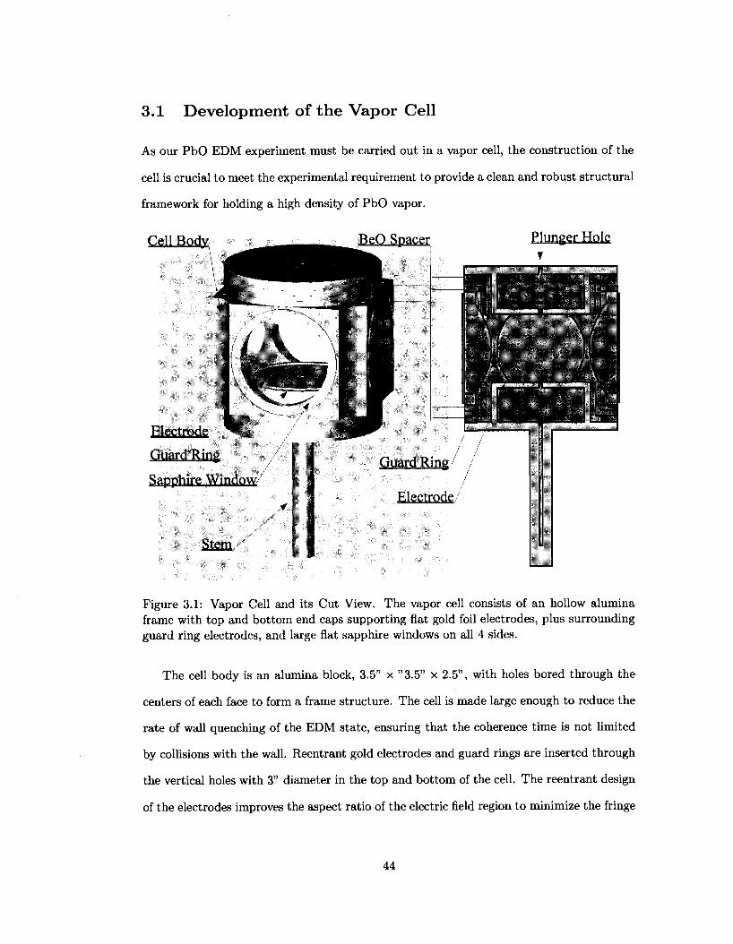
3.1 Development of the Vapor Cell
As our PbO EDM experiment must be carried out in a vapor cell, the construction of the
cell is crucial to meet the experimental requirement to provide a clean and robust structural
framework for holding a high density of PbO vapor.
Figure 3.1: Vapor Cell and its Cut View. The vapor cell consists of an hollow alumina frame with top and bottom end caps supporting flat gold foil electrodes, plus surrounding guard ring electrodes, and large flat sapphire windows on all 4 sides.
The cell body is an alumina block, 3.5" x "3.5" x 2.5", with holes bored through the
centers of each face to form a frame structure. The cell is made large enough to reduce the
rate of wall quenching of the EDM state, ensuring that the coherence time is not limited
by collisions with the wall. Reentrant gold electrodes and guard rings are inserted through
the vertical holes with 3" diameter in the top and bottom of the cell. The reentrant design
of the electrodes improves the aspect ratio of the electric field region to minimize the fringe
44
effect of electric fields due to the finite size of the electrodes, and also provides a metallic
boundary for the molecules, reducing stray fields due to surface charges on the dielectric
parts of the cell. The horizontal holes through the sides are 2" diameter and covered with
sapphire windows using a gold foil bonding technique. A large solid angle of optical access
is necessary to convey a significant fraction of the fluorescence out of the cell, improving
the detection efficiency. Beryllium oxide (BeO) or sapphire electrical insulating spacers are
inserted in the interval between the cell body and the guard ring support, and between the
guard ring and the electrode to diminish leakage currents. The surface of the cell body is
kept clean to avoid contamination which could lead to surface leakage currents. The stem
serves as the PbO reservoir, incorporated with the cell. The depletion of the PbO is slow
enough that we can run our experiments for weeks with no need to refill PbO. In nominal
operation, the temperature of the stem is typically kept tens of degrees below the rest of
the oven in order to remain as a reservoir of PbO and vapor condensation point. The cell
structure is shown in Fig 3.1.
Given the experimental environment of high temperature (T ~ 700° C) and frequent
thermal cycling, the alumina cell body and flat sapphire windows are chosen to satisfy
the material constraints. There are several components that must be bonded with the cell
body, including: sapphire windows, with c-axis normal to the window plane to eliminate
birefringence; re-entrant electrodes; and separate guard-ring electrodes designed to improve
field homogeneity. We have developed a bonding method based on a surface-oxide bond
using gold foil as bonding agent. Such bonds can withstand the high temperature and
aggressive PbO vapor environment and remain mechanically strong, while maintaining
vacuum integrity during frequent thermal cycling. The contact surfaces of the cell body,
electrode support, guard ring support and spacer have been polished to improve the solidity
of the bonding. As discussed in the previous chapter, leakage currents associated with the
applied field should be kept below 10 fj,A under operating conditions to take advantage of
current statistical sensitivity to the electron EDM (see Section 2.6.3). Gold foils are chosen
due to their low vapor pressure at the operating temperatures, preventing formation of
45
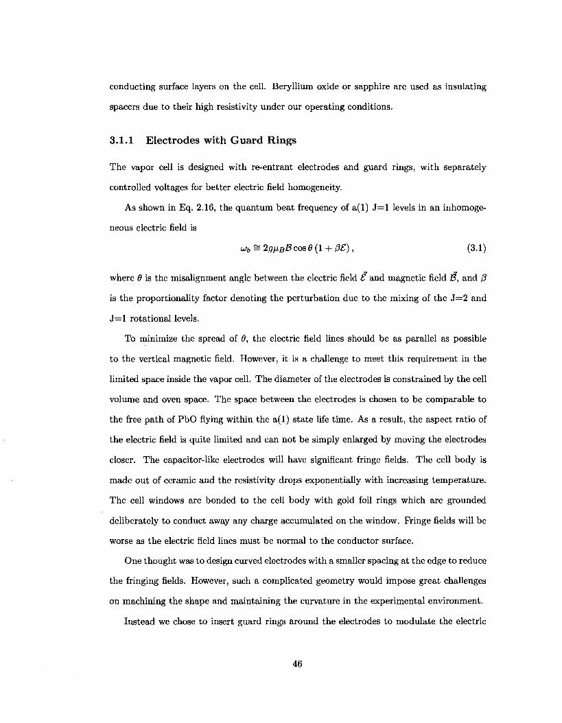
conducting surface layers on the cell. Beryllium oxide or sapphire are used as insulating
spacers due to their high resistivity under our operating conditions.
3.1.1 Electrodes with Guard Rings
The vapor cell is designed with re-entrant electrodes and guard rings, with separately
controlled voltages for better electric field homogeneity.
As shown in Eq. 2.16, the quantum beat frequency of a(l) J = l levels in an inhomoge-
neous electric field is
tJb = 2gfj,BB cos 9 {l + p£), (3.1)
where 0 is the misalignment angle between the electric field £ and magnetic field B, and /?
is the proportionality factor denoting the perturbation due to the mixing of the J=2 and
J = l rotational levels.
To minimize the spread of 0, the electric field lines should be as parallel as possible
to the vertical magnetic field. However, it is a challenge to meet this requirement in the
limited space inside the vapor cell. The diameter of the electrodes is constrained by the cell
volume and oven space. The space between the electrodes is chosen to be comparable to
the free path of PbO flying within the a(l) state life time. As a result, the aspect ratio of
the electric field is quite limited and can not be simply enlarged by moving the electrodes
closer. The capacitor-like electrodes will have significant fringe fields. The cell body is
made out of ceramic and the resistivity drops exponentially with increasing temperature.
The cell windows are bonded to the cell body with gold foil rings which are grounded
deliberately to conduct away any charge accumulated on the window. Fringe fields will be
worse as the electric field lines must be normal to the conductor surface.
One thought was to design curved electrodes with a smaller spacing at the edge to reduce
the fringing fields. However, such a complicated geometry would impose great challenges
on machining the shape and maintaining the curvature in the experimental environment.
Instead we chose to insert guard rings around the electrodes to modulate the electric
46
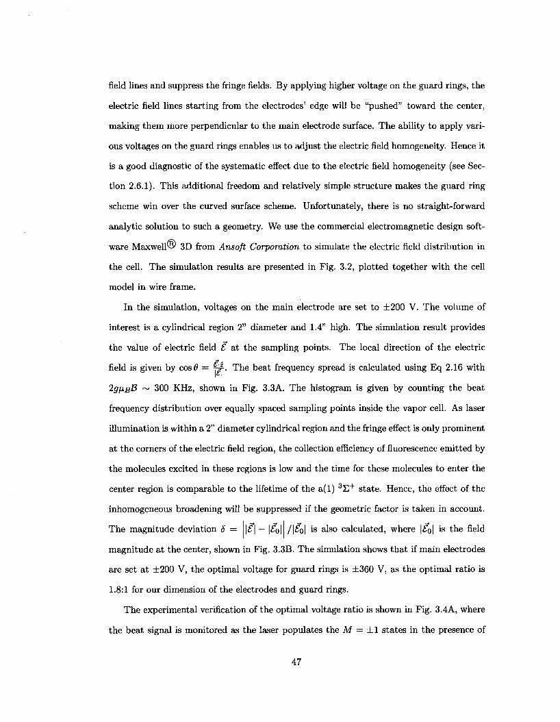
field lines and suppress the fringe fields. By applying higher voltage on the guard rings, the
electric field lines starting from the electrodes' edge will be "pushed" toward the center,
making them more perpendicular to the main electrode surface. The ability to apply vari
ous voltages on the guard rings enables us to adjust the electric field homogeneity. Hence it
is a good diagnostic of the systematic effect due to the electric field homogeneity (see Sec
tion 2.6.1). This additional freedom and relatively simple structure makes the guard ring
scheme win over the curved surface scheme. Unfortunately, there is no straight-forward
analytic solution to such a geometry. We use the commercial electromagnetic design soft
ware Maxwell® 3D from Ansoft Corporation to simulate the electric field distribution in
the cell. The simulation results are presented in Fig. 3.2, plotted together with the cell
model in wire frame.
In the simulation, voltages on the main electrode are set to ±200 V. The volume of
interest is a cylindrical region 2" diameter and 1.4" high. The simulation result provides
the value of electric field £ at the sampling points. The local direction of the electric
field is given by cos# = £#. The beat frequency spread is calculated using Eq 2.16 with
2gnsB ~ 300 KHz, shown in Fig. 3.3A. The histogram is given by counting the beat
frequency distribution over equally spaced sampling points inside the vapor cell. As laser
illumination is within a 2" diameter cylindrical region and the fringe effect is only prominent
at the corners of the electric field region, the collection efficiency of fluorescence emitted by
the molecules excited in these regions is low and the time for these molecules to enter the
center region is comparable to the lifetime of the a(l) 3 £ + state. Hence, the effect of the
inhomogeneous broadening will be suppressed if the geometric factor is taken in account.
The magnitude deviation S = \£\ — \6o\ /\£Q\ is also calculated, where |£o| is the field
magnitude at the center, shown in Fig. 3.3B. The simulation shows that if main electrodes
are set at ±200 V, the optimal voltage for guard rings is ±360 V, as the optimal ratio is
1.8:1 for our dimension of the electrodes and guard rings.
The experimental verification of the optimal voltage ratio is shown in Fig. 3.4A, where
the beat signal is monitored as the laser populates the M = ±1 states in the presence of
47
4.tS50**W3 4-«»»t>00a 4.W2Tfrt4»l
J.(50«*HWS 3.-J7MW00S 3.9W1WW3 3.4M0tt00]
J.O«»7*tM>S
l,e3M**W3 l.fOO'MM* j , * « * + « »
1.13la«*003 ».i$Mt«W>2
I £.32»<*M3
! 6,13W*H»3
S,M43t*O03
S.314«a*a03 }.3793n*)3 5tit3Sa+0Q3
| 4.eot7eHKB
4,*1?7<H003 I 4.»-t2«*»3 • 4.23«7e»0B3
A) B)
C) D)
Figure 3.2: Electric Field in the Cell. The voltage of the guard ring is 375V and main electrode is 200V. A) Top View of E Field Magnitude; B) Side View of E Field Magnitude; C) Side View of Potential; D) Side View of E Field Line.
48
288 290 292 294 296 298 300
0)b (KHz)
200 250 300 350 400 450
Voltage on Guard Ring (V)
Figure 3.3: Electric Field Inhomogeneity in the Cell. Voltages on the main electrode are set to ±200 V. A) Beat frequency spread in the electric field from the simulation result, with nominal beat frequency 300 KHz and guard ring voltage ±360 V. B) Magnitude inhomogeneity is characterized by the magnitude deviation 5 — \£\ — \£Q\ /\£Q\. Simulation
indicates that over as 90% of the cell volume, the magnitude inhomogeneity S is less than 5% in the optimal situation.
various electric fields and the guard rings are fixed at ±135 V. The beat amplitude reaches
maximum when the voltages applied on the main electrodes are around ±75 V respectively,
or 150 V across the electrodes, yielding the optimal voltage ratio of 1.8 as expected.
Furthermore, the beat lifetimes are extracted from the beat signal using the fitting
routine (see Section 2.4.2). The beat lifetime can be interpreted as the coherence time,
directly related to the line width broadening due to the field inhomogeneity. Fig. 3.4B
shows the longest beat lifetime appears around 150 V across the electrodes, coincident
with the result of beat amplitude.
An additional experiment using microwaves to resolve the M = ±1 level carried out by
Paul Hamilton shows the upper limit of broadening due to the electric field inhomogeneity
is less than 1.2%, consistent with the design specification of the electrodes. Vertically
polarized microwaves with low power are used to drive the population of a(l) J = l level
to the J=2 level. As the microwave frequency scans through the resonance condition for
M = ±1 respectively, the disappearance of beats in the J = l state is observed as the
49
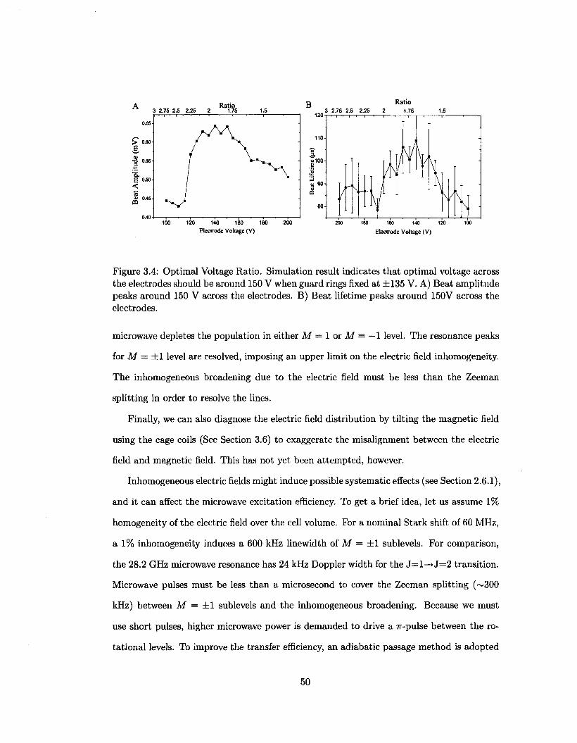
Ratio
U 0.45
to
100 120 140 160 180 200 Electrode Voltage (V)
200 180 160 140 120 100
Electrode Voltage (V)
Figure 3.4: Optimal Voltage Ratio. Simulation result indicates that optimal voltage across the electrodes should be around 150 V when guard rings fixed at ±135 V. A) Beat amplitude peaks around 150 V across the electrodes. B) Beat lifetime peaks around 150V across the electrodes.
microwave depletes the population in either M = 1 or M = — 1 level. The resonance peaks
for M = ±1 level are resolved, imposing an upper limit on the electric field inhomogeneity.
The inhomogeneous broadening due to the electric field must be less than the Zeeman
splitting in order to resolve the lines.
Finally, we can also diagnose the electric field distribution by tilting the magnetic field
using the cage coils (See Section 3.6) to exaggerate the misalignment between the electric
field and magnetic field. This has not yet been attempted, however.
Inhomogeneous electric fields might induce possible systematic effects (see Section 2.6.1),
and it can affect the microwave excitation efficiency. To get a brief idea, let us assume 1%
homogeneity of the electric field over the cell volume. For a nominal Stark shift of 60 MHz,
a 1% inhomogeneity induces a 600 kHz linewidth of M = ±1 sublevels. For comparison,
the 28.2 GHz microwave resonance has 24 kHz Doppler width for the J=l—>J=2 transition.
Microwave pulses must be less than a microsecond to cover the Zeeman splitting (~300
kHz) between M = ±1 sublevels and the inhomogeneous broadening. Because we must
use short pulses, higher microwave power is demanded to drive a 7r-pulse between the ro
tational levels. To improve the transfer efficiency, an adiabatic passage method is adopted
50
which will be discussed in Section 4.3. Nevertheless, we will prefer to control the electric
field inhomogeneity less than 1% over the cell volume. The electric field inhomogeneity
casts technical questions on testing the microwave absorption scheme (see Section 6.2) in
the current cell as well. In this case, the microwaves are in continous-wave mode and
broadened only due to the Doppler effect. Electric field inhomogeneity will diminish the
absorption cross section. When a new generation of long vapor cell is constructed, it will
have rod electrode arrays to apply a cosine-distributed voltage and thus have better electric
field homogeneity.
3.1.2 Leakage Current Suppression
We have taken great caution to minimize the leakage current II associated with the electric
field in our cell. The resistivity of alumina, which is used as the cell body and electrode
support material, is not high enough at high temperatures to keep the leakage currents
below the nominal requirement It, < 10/iA. Therefore, electrical insulation with higher
resistivity and chemical stability in the presence of PbO vapor is needed between the
electrodes and the cell body. These requirements eliminate most insulating materials. In
testing insulating materials, efforts were taken to electrically isolate the vapor cell from the
potential external electrical leakage paths so that we could measure the realistic leakage
current flowing through the cell body. The measured apparent leakage currents are much
higher than the expectation from reported literature of volume resistivity. The resistivity
test conducted in the absence of PbO vapor showed a resistivity of p > 1013 ~ 1014 $7 • cm
at 700°C for BeO. The BeO spacer used in the actual EDM cell has OD 3.5", ID 2.76" and
thickness 1/8", leading to a volume resistance at 1.3 x 10¹⁰ Q,. The closest leakage path is
between the top and bottom guard rings. Two BeO spacers will be sandwiched between
guard rings and the cell body. In the nominal condition with 300 V across the electrodes,
±270 V will be applied on the top and bottom guard rings. The leakage current should be
~ 20 nA, inducing a false EDM of de,leakage ~ 4.3 x 10_27e • cm. Such a systematic error
is higher than our original proposed sensitivity on eEDM and further suppression relies
51
on the iQ-doublet reversal (see Section 2.6.3). This level of leakage current is considered
acceptable but not really satisfying. Even worse, in the presence of PbO vapor in the actual
EDM cell, with BeO spacers inserted in place, we have been unable to obtain consistent
results for /£,. Encouragingly, BeO does not show any signs of reaction with the PbO.
Surface currents might be to blame.
To prevent formation of conducting surface layers on the cell surface, the gold foils are
used as the electrode material. Gold has a low vapor pressure at the operating temperatures
~ 700°C. The cell body surface is kept clean to avoid contamination. Bent quartz tubes
provide structural support for the electrode leads, shown in Fig. 3.5, enabling the leads to
connect from the vapor cell to the outside without touching any high temperature parts
of the oven and without straining the electrode leads. An alumina corner bracket, used
to support the bent tubes, is attached to the outer heat shield, which is supposed to be
much colder than the cell and hence should be a very good insulator. The holes the tubes
go through have a slot to match teeth on the quartz tubes which fix their orientation. A
fork-shaped stop is mounted on the bracket to keep the tubes from sliding in and out.
The assembly with heat shield in place is shown in Fig. 3.6. The cell is supported by
four ceramic poles to minimize the surface of contact to the rest of the apparatus and
eliminate the leakage paths to the chamber body. Ceramic terminal blocks are used to
isolate the out-going leads and connect to the custom nonmagnetic coaxial feedthroughs
(see in Fig. 3.6 and Fig. 3.12). Four channels of trans-impedance amplifiers with isolated
ground, low noise and high sensitivity are used to monitor the leakage current. So far, the
material tests have found the suitable insulating materials are high purity alumina, high
purity sapphire, and Beryllium oxide.
Paul Hamilton has taken leakage current measurements under the typical experimental
conditions in the presence of PbO vapor. High voltage is applied to a single electrode or
guard ring while the rest of the electrodes and guard rings are bundled together and tied to
ground. By monitoring the currents flowing in all electrodes and guard rings, it is possible
to determine the leakage path among the cell, electrodes and guard rings. Currently there
52
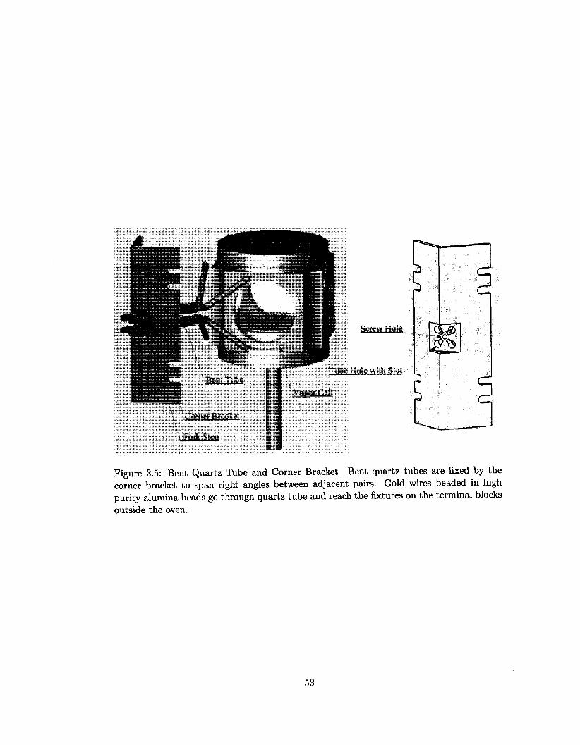
£KaS&! Bent Tube
\Corner Bracket
Fork Stop
mm
Screw Hole
Tube Hole with Slot-
'Vapor Cell
Figure 3.5: Bent Quartz Tube and Corner Bracket. Bent quartz tubes are fixed by the corner bracket to span right angles between adjacent pairs. Gold wires beaded in high purity alumina beads go through quartz tube and reach the fixtures on the terminal blocks outside the oven.
53
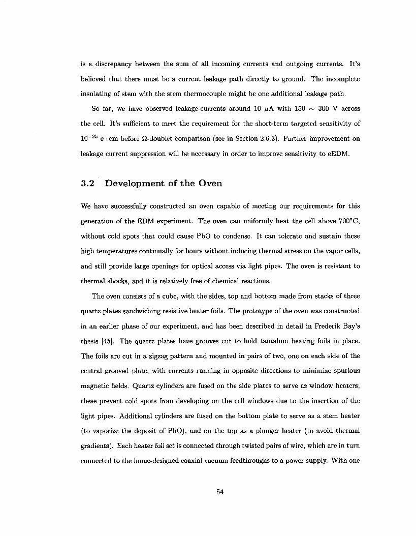
is a discrepancy between the sum of all incoming currents and outgoing currents. It's
believed that there must be a current leakage path directly to ground. The incomplete
insulating of stem with the stem thermocouple might be one additional leakage path.
So far, we have observed leakage-currents around 10 /iA with 150 ~ 300 V across
the cell. It's sufficient to meet the requirement for the short-term targeted sensitivity of
10 - 2 5 e • cm before fi-doublet comparison (see in Section 2.6.3). Further improvement on
leakage current suppression will be necessary in order to improve sensitivity to eEDM.
3.2 Development of the Oven
We have successfully constructed an oven capable of meeting our requirements for this
generation of the EDM experiment. The oven can uniformly heat the cell above 700°C,
without cold spots that could cause PbO to condense. It can tolerate and sustain these
high temperatures continually for hours without inducing thermal stress on the vapor cells,
and still provide large openings for optical access via light pipes. The oven is resistant to
thermal shocks, and it is relatively free of chemical reactions.
The oven consists of a cube, with the sides, top and bottom made from stacks of three
quartz plates sandwiching resistive heater foils. The prototype of the oven was constructed
in an earlier phase of our experiment, and has been described in detail in Frederik Bay's
thesis [45]. The quartz plates have grooves cut to hold tantalum heating foils in place.
The foils are cut in a zigzag pattern and mounted in pairs of two, one on each side of the
central grooved plate, with currents running in opposite directions to minimize spurious
magnetic fields. Quartz cylinders are fused on the side plates to serve as window heaters;
these prevent cold spots from developing on the cell windows due to the insertion of the
light pipes. Additional cylinders are fused on the bottom plate to serve as a stem heater
(to vaporize the deposit of PbO), and on the top as a plunger heater (to avoid thermal
gradients). Each heater foil set is connected through twisted pairs of wire, which are in turn
connected to the home-designed coaxial vacuum feedthroughs to a power supply. With one
54
supply for each heater element, we have independent control of the temperature of each
heating component. The thermocouples are inserted in the space between the stem heater
and the stem, and between the vapor cell and the side heaters, to measure the temperature
distribution inside the oven. These thermocouples are custom made using one gold wire
and one 60/40 gold-palladium alloy wire. The whole oven rests on four ceramic posts to
adjust its vertical position and to electrically isolate it from the rest of the chamber. The
oven, heat shield and the supports are shown in Fig. 3.6.
Figure 3.6: Oven inside the Heat Shield. Three layers of opaque quartz heat shields are held together with ceramic bolts and nuts. The whole oven rests on four ceramic posts. The terminal blocks are mounted on the aluminum bars.
55
Several modification were applied to the current oven. Ceramic glues and high emis-
sivity paints are avoided in the current oven, as there are concerns that the outgasing
from these materials might contaminate the cell surfaces and cause severe leakage current
problems. Opaque quartz is chosen as the oven plate material, instead of the transparent
quartz coated with a high-emissivity paint, to make the temperature of the heater elements
appear more uniform to the cell and detectors.
The heat shields for the current oven are also made out of opaque quartz rather than
thick-metal shields to avoid eddy currents as we switching the heater current on and off.
The oven is enclosed in a heat shield which consists of three layers of opaque quartz
plates, plus reflective metal foils. It is suspected that the low reflectivity of opaque quartz,
together with the enlarged separation of the heater components, causes additional power
consumption, compared with a previous setup using transparent quartz oven plates and
metallic heat shields. The net fraction of radiant energy that escapes a single-layer radiation
shield [54] is given by
( l -nXi + tXi-raQ 2(1 - nr2t
2)
where r\ is the reflectivity of interior surface, r2 is the reflectivity of exterior surface, and
t is the transmissivity of the solid material. The net transmittance through a set of n solid
layers is given by
T = L _ " l + n ( i - l )
The inner surface of the inner heat shield is covered with thin tantalum foils, and the
inner surfaces of two outer shields are covered by copper foils, to increase the surface
reflectivity. Further attempts are being made to investigate the heating efficiency and
blackbody backgrounds.
The entire oven assembly is held together with opaque quartz brackets and ceramic nuts
and bolts. However, there is concern that outgasing of the micro bubbles in the opaque
quartz oxidize the tantalum heating foils and cause them to become brittle and break after
a couple months of heating cycling.
56
Maintaining the temperature stability is important since temperature changes can also
affect the state lifetime T and beat lifetime r (see Section 2.4.2) through changes in the wall
collision or diffusion rate of PbO. In an early era of this experiment, the heaters had to be
turned off during measurements to avoid spurious magnetic field generated by the heater
current flowing around the cell. The new heating scheme, which will be discussed in the
next section, has been used routinely to avoid shutting down the oven and measurements
can be taken at the full duty cycle of laser operation.
3.3 Eddy Current Suppression
Resistive heating turns out to be the only feasible heating scheme in our system to achieve
high temperatures with a homogeneous distribution over the large volume of the oven.
Because of the extreme sensitivity of our experiment to magnetic fields, it is necessary
for the heater currents to be turned off completely during data taking periods, to avoid
generating stray magnetic fields. To maintain the necessary temperature requires high
power, 1000~1500 W, and the heater currents are substantially high (3~5 A). As our laser
system operates at 100 Hz, the heaters must be turned on and off at the same frequency to
achieve a significant duty cycle. To meet these requirements, the heater foils were designed
in a zigzag shape and set together in pairs in close layers, with currents running in opposite
directions, as shown in Fig. 3.3. This keeps the inductance of the heaters very low, and
allows rapid switching while avoiding large eddy-currents being induced in the vacuum can
(see Section 3.2). Previous attempts to switch the heaters involved MOSFET-based circuit
switching linear power supplies. The square shape of the DC current pulses, however,
presented serious problems with persistent eddy currents in the vacuum can.
We implemented a new heating scheme to take data continuously without shutting
down the oven heaters. We drive the heaters with specially-shaped audio frequency pulses
Ih{i) (see Eq. 3.2), generated with low-noise stereo amplifiers (Hafler P3000, P4000, and
QSC units). The input to the amplifier is generated with an arbitrary waveform generator
57
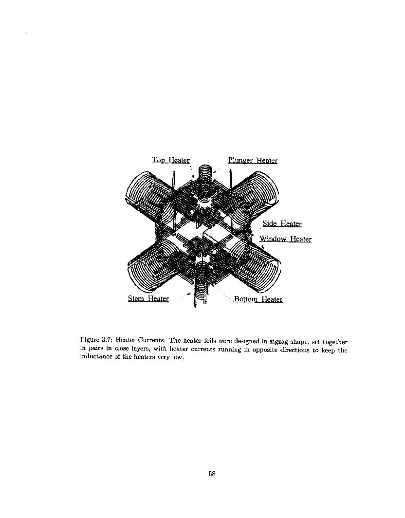
Top Heater Plunger Heater
Side Heater
Window Heater
Stem Heater Bottom Heater
Figure 3.7: Heater Currents. The heater foils were designed in zigzag shape, set together in pairs in close layers, with heater currents running in opposite directions to keep the inductance of the heaters very low.
58
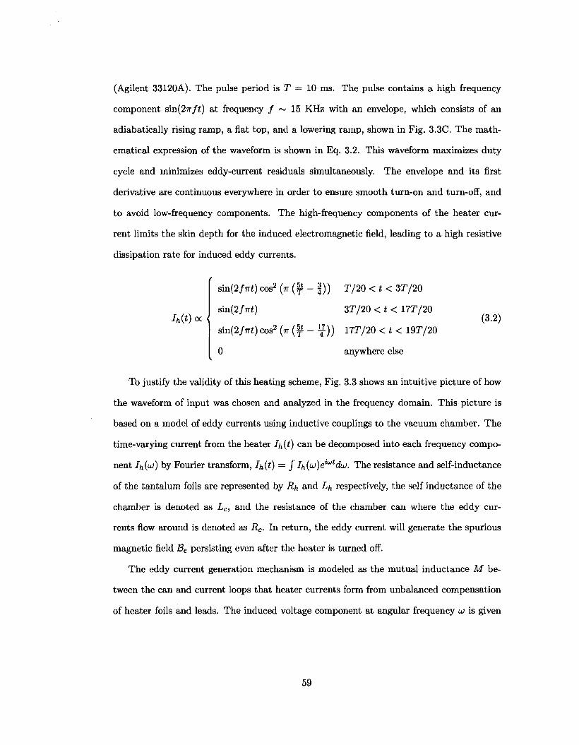
(Agilent 33120A). The pulse period is T = 10 ms. The pulse contains a high frequency
component sin(27r/i) at frequency / ~ 15 KHz with an envelope, which consists of an
adiabatically rising ramp, a flat top, and a lowering ramp, shown in Fig. 3.3C. The math
ematical expression of the waveform is shown in Eq. 3.2. This waveform maximizes duty
cycle and minimizes eddy-current residuals simultaneously. The envelope and its first
derivative are continuous everywhere in order to ensure smooth turn-on and turn-off, and
to avoid low-frequency components. The high-frequency components of the heater cur
rent limits the skin depth for the induced electromagnetic field, leading to a high resistive
dissipation rate for induced eddy currents.
sin(2/7ri) cos2 (ir (§f - f)) T/20 < t < 3T/20
sin(2/7rt) 3T/20 < * < 17T/20 /*(*)«< (3.2)
sin(2/7rt) cos2 (TT ( f - T ) ) 17T/20 < t < 19T/20
0 anywhere else
To justify the validity of this heating scheme, Fig. 3.3 shows an intuitive picture of how
the waveform of input was chosen and analyzed in the frequency domain. This picture is
based on a model of eddy currents using inductive couplings to the vacuum chamber. The
time-varying current from the heater Ih{t) can be decomposed into each frequency compo
nent i/i(u>) by Fourier transform, Ih(t) = J Ih^e^dw. The resistance and self-inductance
of the tantalum foils are represented by Rh and Lh respectively, the self inductance of the
chamber is denoted as Lc, and the resistance of the chamber can where the eddy cur
rents flow around is denoted as Rc. In return, the eddy current will generate the spurious
magnetic field Be persisting even after the heater is turned off.
The eddy current generation mechanism is modeled as the mutual inductance M be
tween the can and current loops that heater currents form from unbalanced compensation
of heater foils and leads. The induced voltage component at angular frequency u is given
59
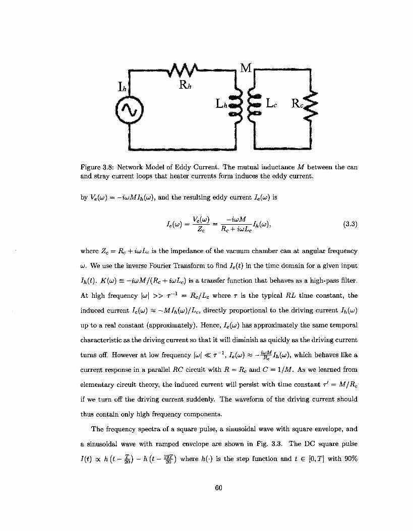
Lc Re,
Figure 3.8: Network Model of Eddy Current. The mutual inductance M between the can and stray current loops that heater currents form induces the eddy current.
by Ve(uj) = —iuMlh{w), and the resulting eddy current Ie(u) is
/«(w) Ve(u) -iu>M
Rc + iuiL, •h{v), (3.3)
where Zc = Rc + iwLc is the impedance of the vacuum chamber can at angular frequency
u). We use the inverse Fourier Transform to find Ie(t) in the time domain for a given input
7/i(i). K(u) = —iuM/(Rc + iuLc) is a transfer function that behaves as a high-pass filter.
At high frequency \u)\ » T _ 1 = Rc/Lc where r is the typical RL time constant, the
induced current Ie{u) « —MIh(uj)/Lc, directly proportional to the driving current i/i(u;)
up to a real constant (approximately). Hence, /e(w) has approximately the same temporal
characteristic as the driving current so that it will diminish as quickly as the driving current
turns off. However at low frequency |u;| -C T - 1 , Ie(ui) w —^^/^(u;), which behaves like a
current response in a parallel RC circuit with R-= Rc and C = 1/M. As we learned from
elementary circuit theory, the induced current will persist with time constant r ' = M/Rc
if we turn off the driving current suddenly. The waveform of the driving current should
thus contain only high frequency components.
The frequency spectra of a square pulse, a sinusoidal wave with square envelope, and
a sinusoidal wave with ramped envelope are shown in Fig. 3.3. The DC square pulse
I(t) oc h(t-£) -h(t- i§f) where h(-) is the step function and t e [0,T] with 90%
60
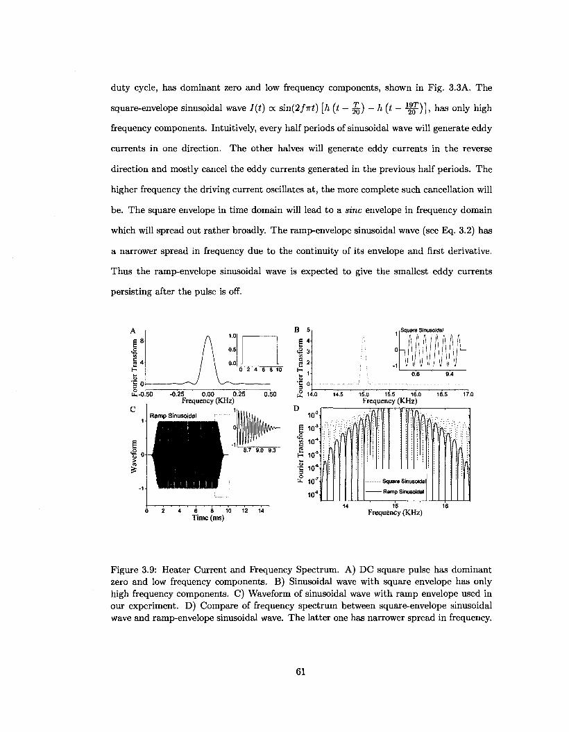
duty cycle, has dominant zero and low frequency components, shown in Fig. 3.3A. The
square-envelope sinusoidal wave I(t) oc sin(2/7ri) [h (t - ^ ) - h (t - ^ f ) ] , has only high
frequency components. Intuitively, every half periods of sinusoidal wave will generate eddy
currents in one direction. The other halves will generate eddy currents in the reverse
direction and mostly cancel the eddy currents generated in the previous half periods. The
higher frequency the driving current oscillates at, the more complete such cancellation will
be. The square envelope in time domain will lead to a sine envelope in frequency domain
which will spread out rather broadly. The ramp-envelope sinusoidal wave (see Eq. 3.2) has
a narrower spread in frequency due to the continuity of its envelope and first derivative.
Thus the ramp-envelope sinusoidal wave is expected to give the smallest eddy currents
persisting after the pulse is off.
Squa
s i re Sinusoidal
SSI 1/lill !
y
• Square Sinusoidal
- Ramp Sinusoidal
4 6 8 10 Time (ms)
Frequency (KHz)
17.0
Figure 3.9: Heater Current and Frequency Spectrum. A) DC square pulse has dominant zero and low frequency components. B) Sinusoidal wave with square envelope has only high frequency components. C) Waveform of sinusoidal wave with ramp envelope used in our experiment. D) Compare of frequency spectrum between square-envelope sinusoidal wave and ramp-envelope sinusoidal wave. The latter one has narrower spread in frequency.
61
To apply this network model to our experiment, we estimate the parameters in Eq. 3.3
based on the geometry of the chamber and oven (see Section 3.2). The typical dimension of
eddy current loop is about 2" in diameter; the skin depth, S = l/y/WfJIa, for the aluminum
chamber at frequency 15 KHz is about 0.8", comparable to the thickness of the chamber;
the resistance of chamber Rc is therefore about 1 fiQ; the self-inductance of the chamber
can Lc is about 1 /iH; the mutual inductance M between the vacuum can and the heater
foil loop is about 0.2 nH, and that between the can and the lead loop is about 0.4 nH.
Hence, the eddy current persisting after the heater is turned off is about 3 mA and the
corresponding residue magnetic field Be at the chamber center is around 10 - 2 mG, when
using the square pulse drive currents. If there is metallic heat shield set close by the heat
foil, the mutual inductance can be as high as 3 nH and induced magnetic field around 2
mG. By contrast, we estimated the magnetic field will be around Be ~ 10 nG in the case
of square-envelope sinusoidal current, and Be < 1 nG using the ramp-envelope sinusoidal
wave now in use.
To study the transient phenomena due to eddy current analytically, we follow a similar
approach as that in Ref [55]. There are also several other approaches to study eddy current
effect [56, 57, 58]. Ref. [55] concerns the mutual-inductance between the drive coil and pick
up coil in the presence of a conductor with application to flaw detection in conductors. Here
we study the relationship between the persistence of the eddy current and the drive current
waveform, and provide the optimization of the waveform to suppress the eddy current.
We use the assumption of a good conductor, make the quasi-static approximation (ap
propriate to the low frequency domain), and apply a Laplace transform on Maxwell's
equations to obtain the vector potential A(f, s), which satisfies
V2A(s) = s/j,crA(s),
where fi is magnetic permeability of the medium, and a is electrical conductivity of the
medium.
62
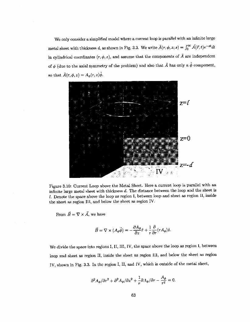
We only consider a simplified model where a current loop is parallel with an infinite large
metal sheet with thickness d, as shown in Fig. 3.3. We write A(r, </>, z; s) = /0°° A(f, t)e~stdt
in cylindrical coordinates (r,(j),z), and assume that the components of A are independent
of <$> (due to the axial symmetry of the problem) and also that A has only a </> component,
so that A(r, </>, z) = A^(r, z)<j>.
Figure 3.10: Current Loop above the Metal Sheet. Here a current loop is parallel with an infinite large metal sheet with thickness d. The distance between the loop and the sheet is I. Denote the space above the loop as region I, between loop and sheet as region II, inside the sheet as region III, and below the sheet as region IV.
From B = V x A, we have
B = V x (A^) = —£r + -frirAJz.
We divide the space into regions I, II, III, IV, the space above the loop as region I, between
loop and sheet as region II, inside the sheet as region III, and below the sheet as region
IV, shown in Fig. 3.3. In the region I, II, and IV, which is outside of the metal sheet,
d2A<p/dr2 + cPAt/dz2 + -dA^/dr - ^ = 0.
63
In the region III, where the metal presents a finite conductivity,
d2A<j>/dr2 + d2A<j>/dz2 + -dA^/dr - 4 * - sftaA^ = 0.
The boundary conditions require that the the vector potential is continuous on the
boundary, and the discontinuity of the divergence of the vector potential on the boundary
is only due to the existence of the current loop between region I and region II.
A«\r,l) = Af\r,ll
§-zAf(r,l)\z=l = ^ ( r . I J U - M«(r - n>),
A^(r,0) = A^\r,0),
AfI\r,-d) = A^\r,-d),
§-/r^)\^=r/r^)\^ d-
In the region III, separation of variables A^(r,z) = R(r)Z(z) gives:
r2d2R/dr2 + rdR/dr -R-a2R = 0,
d2Z/dz2 + a\Z = 0,
where a2 = a2 + s/xa, and a is the "constant" from separation of functions.
The radial equation has the solution R(r) = aJ\(ar) + bYi(ar), where Ji(-) and Yi(-)
are Bessel functions of the first and second kind, respectively, with order 1. For R(r) to be
finite at r = 0, b must be zero. The equation for Z(z) has solution Z(z) = Ae~aiZ + BeaiZ.
The general solution for each region is thus
poo
A+{r,z) = / [B(a)e~az + C{a)eaz] Ji{ar)da. Jo
64
In each region,
/*oo
4p(r,z) = J B1(a)e-Q 2Ji(ar)da,
/•OO
Af\r, z) = J [B2(a)e-az + C2{a)eaz] J^da,
^U\r,z) = J [B3(a)e-a* + C3(a)ea*} ^ ( a r jda , / 'OO
AVv)(TjZ)= C4(a)ea zJi(ar)da.
Applying the boundary conditions:
Bie-al = B2e-al + C2eal,
-Bxe~al = - E 2 e - a / + C2eal - fiIr0Ji(ar),
B2 + C2 = B3 + C3,
-B2 + C2 = —(-B3 + C3), a
B3eaid + C3e-aid = C4e-ad,
-aiB3eaid + aiC3e-aid = aCAe-ad,
and solving the above equations, we obtain
Bi(a) = -fJ,Ir0Ji{ar0) • al (a2 - a2) + (a2 - a\)e2^d _al
-(ai - a)2 + (ax + a)2e2^d
The first term in this expression is simply, the static magnetic field generated by the current
loop without the perturbation from the existence of the metal sheet. The effect of the metal
sheet is characterized by the second term which gives rise to the vector potential AA, '
due to the eddy currents:
A A , = fil(s)r0
/•OO
/ Ji{ar0)Ji{ar)t Jo
-aU+l) ( a 2 - a 2 ) + ( a 2 - a 2 ) e 2 ^ -{ax - a)2 + (ai + a)
2e2a^d da.
65
We define the kernel function K(s) as
( a 2 - a 2 ) + ( a 2 - g 2 ) e 2 ^ W ( a i - a ) 2 - ( a i + a ) 2 e 2 " i r f '
In the time domain, the transient eddy current can be expressed as
AA^t) = - - /wo / Ji(aro)Ji(ar)e-a(2+ ' )£-1[7(s) * K(s)]da, (3.4)
where the "*" indicates a convolution between heater current and the kernel function, and
we exchanged the order of integration without strict justification. The above results are
exact up to the quasi-static approximation, yet it is hard to get an intuitive idea how to
optimize the current pulse from this expression. We make the rough approximation of a
good conductor, equivalent to the assumption |cvi| » a, such that
(' < * 2 ( l - £ ) 2 [ l - ( ^ ) 2e - W ] a> + s„o- V*>
This shows the familiar result of Eq. 3.3, where iu> is replaced by s. The inverse Laplace
transform of K (s) yields the result
The convolution of the Dirac delta function with the driving current simply gives the
component proportional to the driving current, which will vanish together with the turn-off
of driving current. The second term in K(t) produces a lasting decay component. Over
the interesting spatial scale, we can ignore the contribution from a » Z_1 due to the
factor of e~al in Eq. 3.4, so that the condition |ai | >> a will always hold as we recall
that a\ = a2 + s/j,a. a - 1 can be treated as the characteristic scale of the system. Prom
the equation above, we observe that the time scale over which eddy currents persist is
re ~ fj,a/a2, which will be substantially long for small a.
66
To further investigate the situation, we make the approximation
K(s) « 1 - — , (3.6) sfia
2
appropriate for -—^ «; 1, and simplify the problem by only considering the magnetic field
along the symmetry axis r = 0. In this case
AB{t,r = 0) = £-1{B(s)\,
A5(s , r = 0) = --pro / ae-a^z+l^J1(ar0)I(s)K{s)daz 2 Jo
1 /-oo 2
w =-lir0 / a e - a ^ + ' ) j 1 ( a r 0 ) / ( s ) ( - l + —)daz 2 Jo s/ia
= Bi(s,r = 0) + B2(s,r = 0).
Here
Bi(s,r = 0) = -^rnr0 l°° ae'a^z+l^ Ji{aro)daz; 2 Jo
B2(s,r = 0) = ^ - ^ - !°°a3e-^z+l^Ji(ar0)daz 2<T s Jo
_J(s)3r02 [(/ + * ) 2 - r 2 ]
s 2a [r2 + (/ + ^)2]7/2 •
Notice that the upper bounds of the integration have been extended to the infinity approx
imately as ea(z+v> term makes the contribution from large a negligible.
B\(s) gives rise to the same temporal character as the driven pulse I(s), reflecting the
damping effect due to the adjacent metal sheet. However, we are more interested in the
second term B2(s), which governs the residual magnetic field during the times that the
driving pulse is off. The temporal characteristic of the residual magnetic field B2 (t) due to
eddy current is
B2(t) = C~l [B2{s)} oc C~l I(s) ^=J*I(t')dt'. (3.7)
67
We wish minimize \f0 I{T)CLT\ in the period of pulse T under the constraint of
/ I2(t')dt' = P-T/Rh, Jo
where Rh is the resistance of the heater, and P is the total power the heater consumes.
It is easy to see that only an oscillatory waveform without a DC component can make
fil(t')dt' = 0.
A DC square pulse I(t) oc h(t - ^ ) — h(t - ^§j-), will result in a non-zero temporal
integral of the current, which in turn induce a long-persisting eddy current. Yet if we apply
a sinusoidal wave with a square pulse envelope, I(t) ex sin(2/7rt) [h (t — ^g) — h(t - n§y-)],
the integral of Eq. 3.7 will give ~ sin f §^y- J sin(/7rT)//7r, suppressed by using a high
frequency, which justifies our original thoughts. If we introduce a ramp in the pulse's
rising and falling edges using one quarter period of sine function as the envelope, to make
overall waveform have the envelope and its first derivative continuous everywhere (see
Eq. 3.2 and Fig. 3.3), the integral of Eq. 3.7 will give
/ /TTTN / 3 / T T T \ (\1fnT\ /19/TrTY cos^J+co%-io-J-cosl-lo-J-cos(,^o-J. '
with higher order of suppression as t(f'i'fi_2h) •
However, Eq. 3.7 is rather a simplified model to measure the eddy current persistence
and can not justify the superior performance of ramp-envelope sinusoidal wave over the
square-envelope sinusoidal wave as both can give the zero result of the integral of Eq. 3.7
with appropriate choice of the frequency. We need to consider the transient phenomena
due to the discontinuity during switch-on and switch-off. The square pulse case is studied
in Ref. [59]. Let us examine the approximation on Eq. 3.5 again. Contrary to the condition
leading to Eq. 3.6, for large a,
25 4/TT ( /2T2 - 25)
68
Althoug the integral in Eq. 3.4 is suppressed by e for large a, according to the property
of the Laplace transform,
= /(»>(*)
with F(s) = C [/(£)]. In our case, the waveform is flat initially, so /(0~) = 0 and jW(0~) —
0 for all i G Af. The discontinuity of the differentiation of the waveform in time will
contribute significantly to the behavior of eddy current as the next order differentiation
will be a delta function. It is hard to get an analytical solution to complete the rest
of integration in Eq. 3.4 and we have to resort to the numerical method. A numerical
calculation based on the exact solution Eq. 3.4 confirms a significant suppression of residual
eddy currents using ramp-envelope waveform. The magnetic field due to the residual eddy
current is smaller than O.lnG in the same geometry we used in the previous estimation.
The conclusion we draw from above analysis justifies our original thoughts.
The ramp-envelope waveform has been applied to the heating scheme. The waveform
with 16000 sample points is generated by Mathematica program and saved in spread sheet
format. Agilent software IntuiLink loads the spread sheet and sends the waveform to
Agilent arbitrary waveform generator 33120A. The output of Agilent 33120A is fed through
a low-pass filter box to smooth away the digitized steps in the waveform, then goes into
the input ports of audio amplifiers to drive the heaters.
3.4 Plunger
The vapor cell is held together firmly by gravity and by the force from the plunger. The
cell is assembled in the open air environment so it is necessary to evacuate the vapor cell
through a small hole opened on the top electrodes (see Fig. 3.1) at low temperature before
PbO vaporizes. It has been observed that gaseous contaminants such as water vapor and
carbon dioxide, quench the a(l) PbO state and shorten the state life time. The plunger
snF{s) - sn-lf{Q-) / ("-^((T)
69
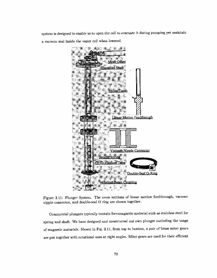
system is designed to enable us to open the cell to evacuate it during pumping yet maintain
a vacuum seal inside the vapor cell when lowered.
;• Pi
' i' 'J i' I *
f ! .' i
'---. Miter Gears
Threaded Shaft
Spline Tooth
i Linear Motion Feedthrough
I i / j
"W<
mm>
Vacuum Nipple Connector
Bron7e Spring
OF40 Vncuum Tube
nonhle-Seal O-Ring
Helical Beam Coupling
Figure 3.11: Plunger System. The cross sections of linear motion feedthrough, vacuum nipple connector, and double-seal O ring are shown together.
Commercial plungers typically contain ferromagnetic material such as stainless steel for
spring and shaft. We have designed and constructed our own plunger excluding the usage
of magnetic materials. Shown in Fig. 3.11, from top to bottom, a pair of brass miter gears
are put together with rotational axes at right angles. Miter gears are used for their efficient
70
transmission of motion between intersecting shafts at a right angle. The horizontal shaft
extends outside of the magnetic shields and is turned by hand. A threaded vertical shaft
driven by the miter gear is coupled to a linear motion feedthrough to convert the rotation
to linear translation in the up or down direction. A spline tooth extruded sideways from
the linear motion feedthrough is constrained in a slot to limit the displacement range. The
axial seal and radial seal are provided by the O-rings sitting inside the vacuum nipple
connector as the mid-part of the plunger system, provide good vacuum seal and allow the
translation feed into the vacuum chamber by shaft. Double-seal O rings with X-shape cross
section are used for the axial seal around the movable shaft. An aluminum QF-40 vacuum
tube is used to mount the plunger system to the top plate of vacuum chamber. Inside the
tube, a flexible coupling is used to allow some compression on the cell. Phosphor bronze
spring (alloy ASTM B 159, contain Fe < 0.1%) and aluminum helical beam couplings are
used in place of steel counterparts used in commercial products. An alumina rod with a
polished end is coupled to the shaft and provides the seal to the hole on the top electrode
plate. The plunger heater around the rod prevents the thermal gradients to the rest of the
oven when the oven is heated up.
3.5 Non-Magnetic BNC Feedthrough
Commercial vacuum co-axial feedthroughs typically contain some ferromagnetic compo
nents or plating material, thus custom co-axial feedthroughs were designed to replace
them. The co-axial feedthrough consists of an outer brass ground tube and center pin to
conduct the electrical signal through the vacuum chamber, as shown in Fig. 3.12. One end
of the ground tube is open to the air with an inner thread to mate with a BNC plug, and
the other half has outer threads such that hex nuts can be used to fasten the tube as it
goes through the holes on an alumina QF-40 flange. A brass rod serving as the ground
lead is attached to a hex nut mounted on the vacuum end of the tube. Additional nuts are
used to lock down the BNC plug and ground lead nut. The center pin is made out of 2-56
71
threaded rods with a nut and a smooth sleeve tube weld close to one end. The center pin
goes through Delrin spacer and bushing with a small O-ring sandwiched between the spacer
and bushing to provide axial sealing. Some spacers and bushings were made out of Teflon.
Either material works well. The bushing is pushed against the shoulder inside the ground
tube with another O-ring sandwiched in between to provide radial sealing. In a symmetric
way, there are similar sealing components on the other side of the shoulder. Then a hex nut
is mounted along the center pin to fasten the bushings together. Further in the very end,
an alumina washer fixed with two 2-56 nuts serves as a centering spacer. Barrel connectors
are mounted to the center pin and the ground pin to connect the leads coming out from the
oven. Quartz sleeves are sometimes inserted around the barrel connectors as insulation.
Each QF-40 flange contains three BNC feedtrhoughs to save space. Alumina is chosen
as the flange material to insulate the feedthroughs. The outer surface of the alumina QF-40
flange is well polished to provide good contact surface for the O-ring which is embedded
in the groove located at the outer shoulder of the ground tube. The flat part of flange is
made thicker to strengthen the flange and has a tilt edge to adapt easily with the standard
vacuum fastening components. The groove is compatible to the standard centering O-ring.
Aluminum supporting rings are used to hold the flange onto the vacuum chamber wall. A
small cross-section O-ring with diameter slightly smaller than the flange is placed between
the flange and the aluminum supporting ring to even out the pressure and avoid cracking
the flange. All BNC plugs and coaxial cables connected to the feedthroughs inside the
shield are free from ferromagnetic materials.
3.6 Magnetic Shield and Magnetic Coils
Magnetic shields eliminate problems due to ambient magnetic field fluctuations and field
gradients. Mu-metal is a high permeability ferromagnetic material commercially available
for magnetic shielding. Multilayer Mu-metal shields are used in our experiment to im
prove the shielding effect. Considerable engineering and construction efforts were taken to
72
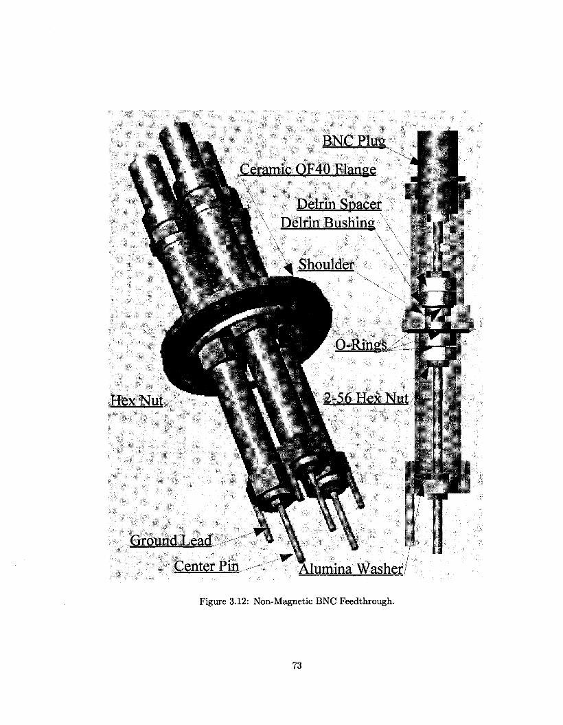
Hex Nut
BNCPlug
Ceramic OF40 Flange
Delrin Spacer Delrin Bushing
Shoulder
O-Rings
2-56 Hex Nut j j
wJslliiSaB
Ground Lead
Center Pin
• M B
if Alumina Washer/
Figure 3.12: Non-Magnetic BNC Feedthrough.
73
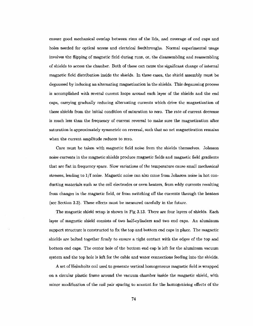
ensure good mechanical overlap between rims of the lids, and coverage of end caps and
holes needed for optical access and electrical feedthroughs. Normal experimental usage
involves the flipping of magnetic field during runs, or, the disassembling and reassembling
of shields to access the chamber. Both of these can cause the significant change of internal
magnetic field distribution inside the shields. In these cases, the shield assembly must be
degaussed by inducing an alternating magnetization in the shields. This degaussing process
is accomplished with several current loops around each layer of the shields and the end
caps, carrying gradually reducing alternating currents which drive the magnetization of
these shields from the initial condition of saturation to zero. The rate of current decrease
is much less than the frequency of current reversal to make sure the magnetization after
saturation is approximately symmetric on reversal, such that no net magnetization remains
when the current amplitude reduces to zero.
Care must be taken with magnetic field noise from the shields themselves. Johnson
noise currents in the magnetic shields produce magnetic fields and magnetic field gradients
that are flat in frequency space. Slow variations of the temperature cause small mechanical
stresses, leading to 1/f noise. Magnetic noise can also come from Johnson noise in hot con
ducting materials such as the cell electrodes or oven heaters, from eddy currents resulting
from changes in the magnetic field, or from switching off the currents through the heaters
(see Section 3.3). These effects must be measured carefully in the future.
The magnetic shield setup is shown in Fig 3.13. There are four layers of shields. Each
layer of magnetic shield consists of two half-cylinders and two end caps. An aluminum
support structure is constructed to fix the top and bottom end caps in place. The magnetic
shields are bolted together firmly to ensure a tight contact with the edges of the top and
bottom end caps. The center hole of the bottom end cap is left for the aluminum vacuum
system and the top hole is left for the cable and water connections feeding into the shields.
A set of Helmholtz coil used to generate vertical homogeneous magnetic field is wrapped
on a circular plastic frame around the vacuum chamber inside the magnetic shield, with
minor modification of the coil pair spacing to account for the homogenizing effects of the
74
1 "I •
| If S;|
* ' ""I
Figure 3.13: Magnetic Shields and Aluminum Supports
75
magnetic shielding. Additional anti-Helmholtz coils are used to generate the magnetic
gradient in the z direction. Two pairs of auxiliary coils in anti-Helmholtz configuration,
with a '"cosine"' distribution winding to form a current cage around the chamber, are
used to generate magnetic gradients in the x and y directions. Two similar cage coils,
in Helmholtz configuration, are used to generate the magnetic field along the x and y
direction, in order to tip the magnetic field when adjusting the alignment of the magnetic
field and the electric field. All of these auxiliary coils are also used as diagnostics for
systematics.
3.7 High Voltage Amplifier
The Q-doublet feature provides excellent diagnostics for systematics related to the electric
field flipping, as we can simply change the microwave frequency to address the different fl-
doublet pairs and flip the intra-molecular electric field without any change to the external
electric field. The near equality of the g-factors of the polarized levels in PbO a(l) state
indicates the possibility to suppress systematic effects substantially (see Section 2.6.3).
Thus, it will be helpful to provide nearly perfect electric field reversal. We targeted a
goal of E/5E «C 10~5, to take full advantage of the systematic suppression mechanism.
With a nominal value of 300 V applied to the field electrodes, the voltage discrepancy in
reversal should be kept much smaller than 30 mV, say below tens of millivolt, to achieve
this condition.
We require a linear amplifier capable of providing an output in excess of ±400 V, across
a predominantly capacitive load, with changes on the time scale of milliseconds. In order to
meet the experimental requirement of flipping the high voltage to high accuracy in a time
scale shorter than the ambient magnetic field drift, the challenge is to build a high voltage
amplifier that can boost the output of a voltage standard with excellent reversibility and
stability. Previous attempts using commercial HV amplifier chips provided unsatisfactory
results, due to the high cost and fragility of these chips. Here a simple circuit, described
76
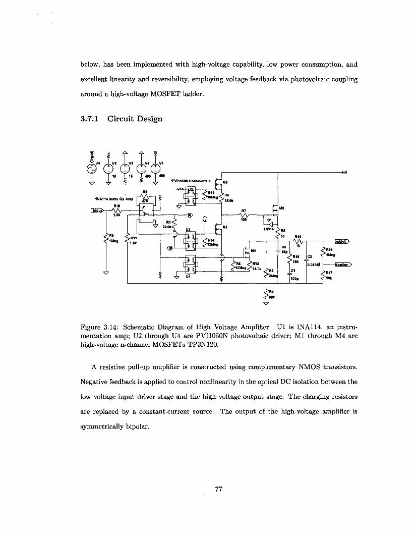
below, has been implemented with high-voltage capability, low power consumption, and
excellent linearity and reversibility, employing voltage feedback via photovoltaic coupling
around a high-voltage MOSFET ladder.
3.7.1 Circuit Design
15 J 400 I «M> [ g % X *PVI1050N Photovoltaic i*-^
*INA114lMttuOpAmp
R10
QBH>T-A/V
&» &
C7
<t L a f J „>12M«||
<r 3E lonltor >
Figure 3.14: Schematic Diagram of High Voltage Amplifier. Ul is INA114, an instrumentation amp; U2 through U4 are PVI1050N photovoltaic driver; Ml through M4 are high-voltage n-channel MOSFETs TP3N120.
A resistive pull-up amplifier is constructed using complementary NMOS transistors.
Negative feedback is applied to control nonlinearity in the optical DC isolation between the
low voltage input driver stage and the high voltage output stage. The charging resistors
are replaced by a constant-current source. The output of the high-voltage amplifier is
symmetrically bipolar.
77
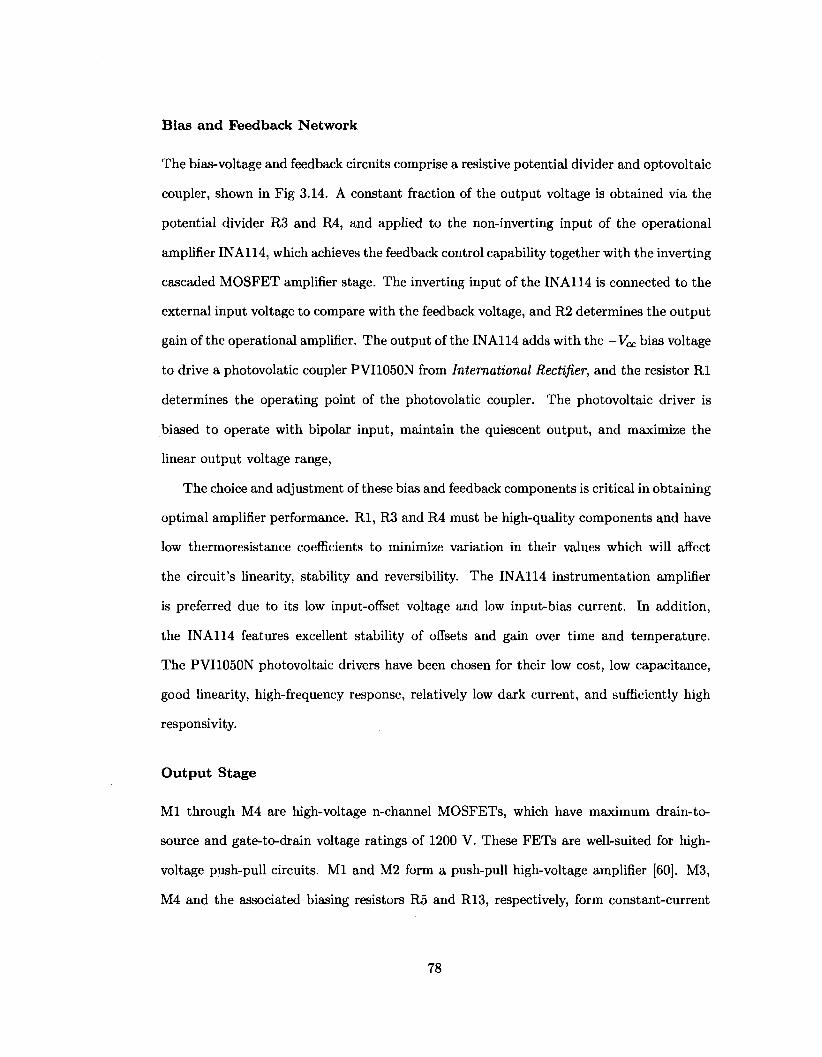
Bias and Feedback Network
The bias-voltage and feedback circuits comprise a resistive potential divider and optovoltaic
coupler, shown in Fig 3.14. A constant fraction of the output voltage is obtained via the
potential divider R3 and R4, and applied to the non-inverting input of the operational
amplifier INA114, which achieves the feedback control capability together with the inverting
cascaded MOSFET amplifier stage. The inverting input of the INA114 is connected to the
external input voltage to compare with the feedback voltage, and R2 determines the output
gain of the operational amplifier. The output of the INA114 adds with the —VQC bias voltage
to drive a photovolatic coupler PVI1050N from International Rectifier, and the resistor Rl
determines the operating point of the photovolatic coupler. The photovoltaic driver is
biased to operate with bipolar input, maintain the quiescent output, and maximize the
linear output voltage range,
The choice and adjustment of these bias and feedback components is critical in obtaining
optimal amplifier performance. Rl, R3 and R4 must be high-quality components and have
low thermoresistance coefficients to minimize variation in their values which will affect
the circuit's linearity, stability and reversibility. The INA114 instrumentation amplifier
is preferred due to its low input-offset voltage and low input-bias current. In addition,
the INA114 features excellent stability of offsets and gain over time and temperature.
The PVI1050N photovoltaic drivers have been chosen for their low cost, low capacitance,
good linearity, high-frequency response, relatively low dark current, and sufficiently high
responsivity.
Output Stage
Ml through M4 are high-voltage n-channel MOSFETs, which have maximum drain-to-
source and gate-to-drain voltage ratings of 1200 V. These FETs are well-suited for high-
voltage push-pull circuits. Ml and M2 form a push-pull high-voltage amplifier [60]. M3,
M4 and the associated biasing resistors R5 and R13, respectively, form constant-current
78
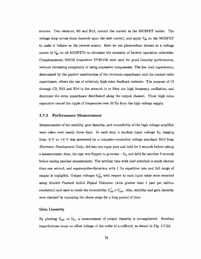
sources. Two resistors, R5 and R13, control the current in the MOSFET ladder. The
voltage drop across them depends upon the sink current, and apply V^a on the MOSFET
to make it behave as the current source. Here we use photovoltaic drivers as a voltage
source of Igs on all MOSFETs to eliminate the necessity of battery operation otherwise.
Complementary NMOS transistors TP3N120 were used for good linearity performance,
without increasing complexity or using expensive components. The low load capacitance,
determined by the parallel combination of the electrode capacitance and the coaxial cable
capacitance, allows the use of relatively high-value feedback resistors. The purpose of CI
through C3, R15 and R18 in the network is to filter out high frequency oscillation, and
dominate the stray capacitance distributed along the output channel. These high value
capacitors cancel the ripple of frequencies over 10 Hz from the high voltage supply.
3.7.2 Performance Measurement
Measurements of the stability, gain linearity, and reversibility of the high voltage amplifier
were taken over nearly three days. In each step, a random input voltage Mn ranging
from -8 V to +8 V was generated by a computer-controlled voltage standard 501J from
Electronic Development Corp., fed into the input port and held for 5 seconds before taking
a measurement; then, the sign was flipped to generate — Vm and held for another 5 seconds
before taking another measurement. The settling time with load attached is much shorter
than one second, and square-pulse-distortion with 1 Hz repetitive rate and full range of
output is negligible. Output voltages V^ t with respect to each input value were recorded
using Hewlett Packard 3455A Digital Voltmeter (with greater than 1 part per million
resolution) and used to check the reversibility V^ t + V^~t. Also, stability and gain linearity
were checked by repeating the above steps for a long period of time.
Gain Linearity
By plotting Vout vs 14n, a measurement of output linearity is accomplished. Residual
imperfections cause an offset voltage of the order of a millivolt, as shown in Fig. 3.7.2A.
79
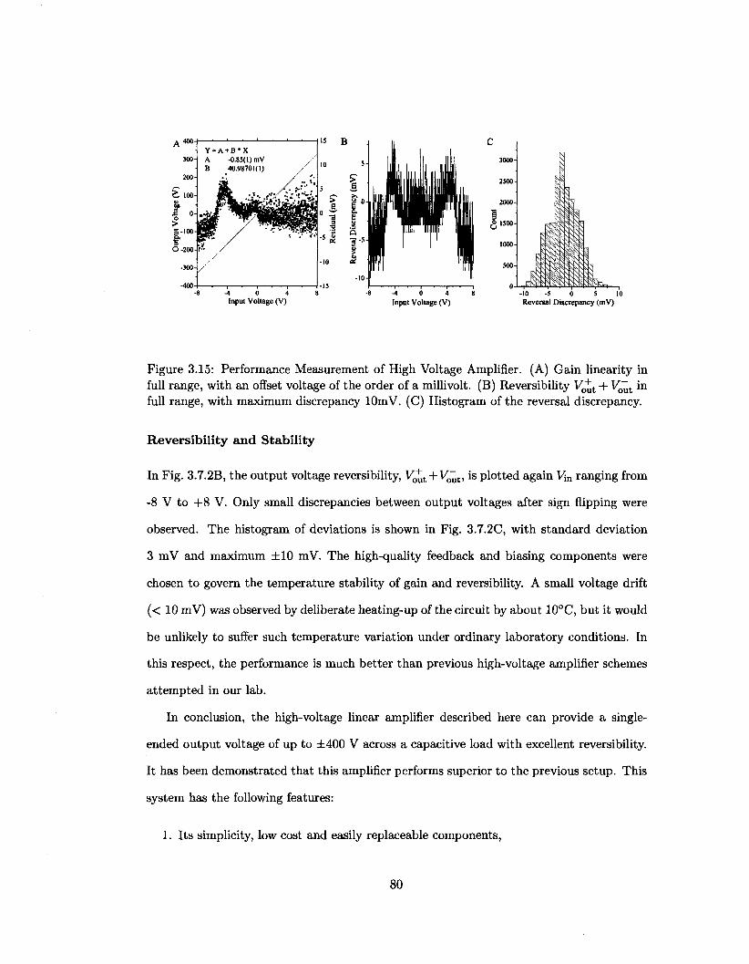
Figure 3.15: Performance Measurement of High Voltage Amplifier. (A) Gain linearity in full range, with an offset voltage of the order of a millivolt. (B) Reversibility V^ t + V ~t in full range, with maximum discrepancy lOmV. (C) Histogram of the reversal discrepancy.
Reversibility and Stability
In Fig. 3.7.2B, the output voltage reversibility, V^ t + V^~t, is plotted again V;n ranging from
-8 V to +8 V. Only small discrepancies between output voltages after sign flipping were
observed. The histogram of deviations is shown in Fig. 3.7.2C, with standard deviation
3 mV and maximum ±10 mV. The high-quality feedback and biasing components were
chosen to govern the temperature stability of gain and reversibility. A small voltage drift
(< 10 mV) was observed by deliberate heating-up of the circuit by about 10°C, but it would
be unlikely to suffer such temperature variation under ordinary laboratory conditions. In
this respect, the performance is much better than previous high-voltage amplifier schemes
attempted in our lab.
In conclusion, the high-voltage linear amplifier described here can provide a single-
ended output voltage of up to ±400 V across a capacitive load with excellent reversibility.
It has been demonstrated that this amplifier performs superior to the previous setup. This
system has the following features:
1. Its simplicity, low cost and easily replaceable components,
80
2. Optical coupling allows a high degree of adjustability and utilization of contemporary
cheap MOSFET components,
3. Improved linearity and reversibility performance due to high-quality feedback and
deep internal gain stages.
Currently, we still work with the unit using the commercial amplifier chip as the com
mercial chips have much faster frequency response and can be used for high frequency Stark
modulation. For final EDM data, we will swap in the new high-voltage linear amplifier.
3.8 Laser Excitation and Fluorescence Detection
3.8.1 Laser Excitation
A pulsed dye laser is used to drive the weakly-allowed transition X(0) —• a(l) in the first
step of the laser-microwave double resonance. A SCANmate 2E dye laser from Lambda
Physik is equipped with components to suppress the amplified spontaneous emission (ASE)
and the output bandwidth of the laser is limited to ~1 GHz, which is comparable to the
Doppler width experienced by PbO molecules at 700° C. An Nd:YAG laser from Spectra
Physics serves as the pump laser generating pulses at 532 nm wavelength as the second
harmonics of 1064 nm, with 7~10 ns pulse width, 100 mJ per pulse, and a repetition rate
of 100 Hz (custom design using two pairs of flash lamps firing alternately, with repetition
rate of 50 Hz). The Q-switch triggering TTL pulse of the Nd:YAG laser serves as the
timing reference for the rest of the experiment.
Shown in Fig. 2.3, the laser beam coming out of the dye laser is first expanded by
a collimating telescope. As the original laser beam is vertically polarized, a A/2 wave-
plate is used to rotate the polarization direction and a Glan-Laser prism inserted to ensure
the transmitted beam is linearly polarized along the desired direction. The laser beam is
expanded further by another collimating telescope to ~ 2" diameter before going through
the 2" diameter quartz light pipe.
81
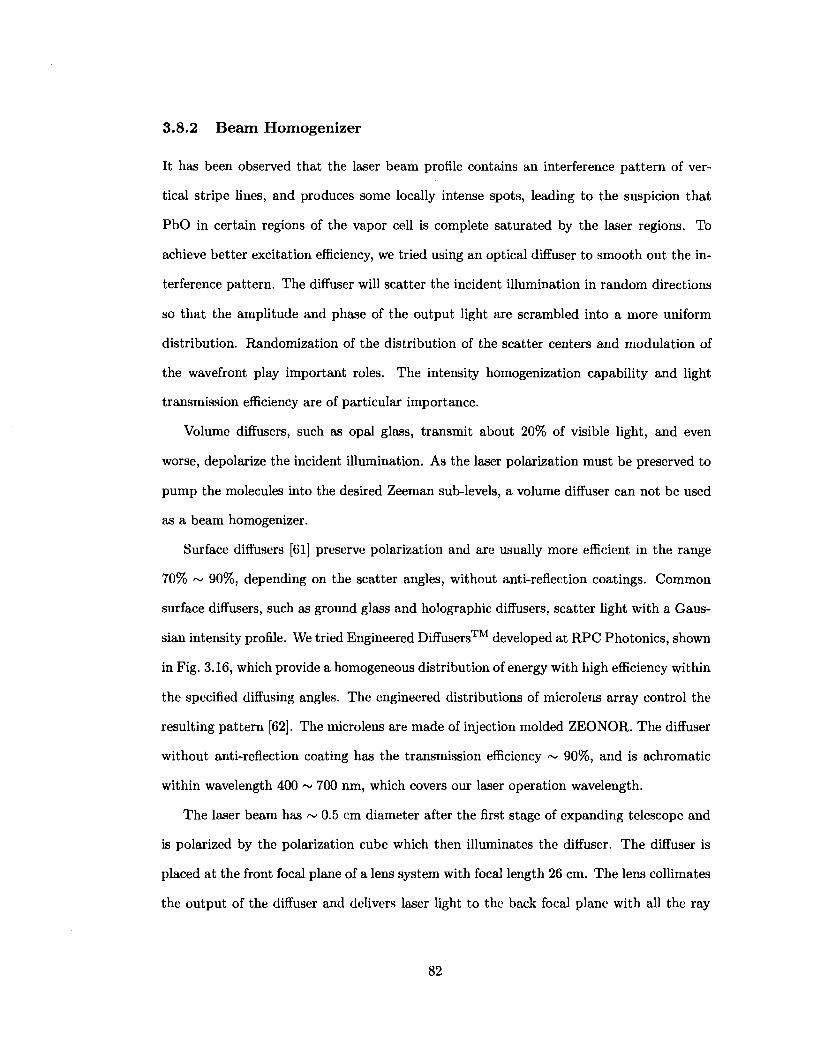
3.8.2 B e a m Homogenizer
It has been observed that the laser beam profile contains an interference pattern of ver
tical stripe lines, and produces some locally intense spots, leading to the suspicion that
PbO in certain regions of the vapor cell is complete saturated by the laser regions. To
achieve better excitation efficiency, we tried using an optical diffuser to smooth out the in
terference pattern. The diffuser will scatter the incident illumination in random directions
so that the amplitude and phase of the output light are scrambled into a more uniform
distribution. Randomization of the distribution of the scatter centers and modulation of
the wavefront play important roles. The intensity homogenization capability and light
transmission efficiency are of particular importance.
Volume diffusers, such as opal glass, transmit about 20% of visible light, and even
worse, depolarize the incident illumination. As the laser polarization must be preserved to
pump the molecules into the desired Zeeman sub-levels, a volume diffuser can not be used
as a beam homogenizer.
Surface diffusers [61] preserve polarization and are usually more efficient in the range
70% ~ 90%, depending on the scatter angles, without anti-reflection coatings. Common
surface diffusers, such as ground glass and holographic diffusers, scatter light with a Gaus
sian intensity profile. We tried Engineered Diffusers™ developed at RPC Photonics, shown
in Fig. 3.16, which provide a homogeneous distribution of energy with high efficiency within
the specified diffusing angles. The engineered distributions of microlens array control the
resulting pattern [62]. The microlens are made of injection molded ZEONOR. The diffuser
without anti-reflection coating has the transmission efficiency ~ 90%, and is achromatic
within wavelength 400 ~ 700 nm, which covers our laser operation wavelength.
The laser beam has ~ 0.5 cm diameter after the first stage of expanding telescope and
is polarized by the polarization cube which then illuminates the diffuser. The diffuser is
placed at the front focal plane of a lens system with focal length 26 cm. The lens collimates
the output of the diffuser and delivers laser light to the back focal plane with all the ray
82
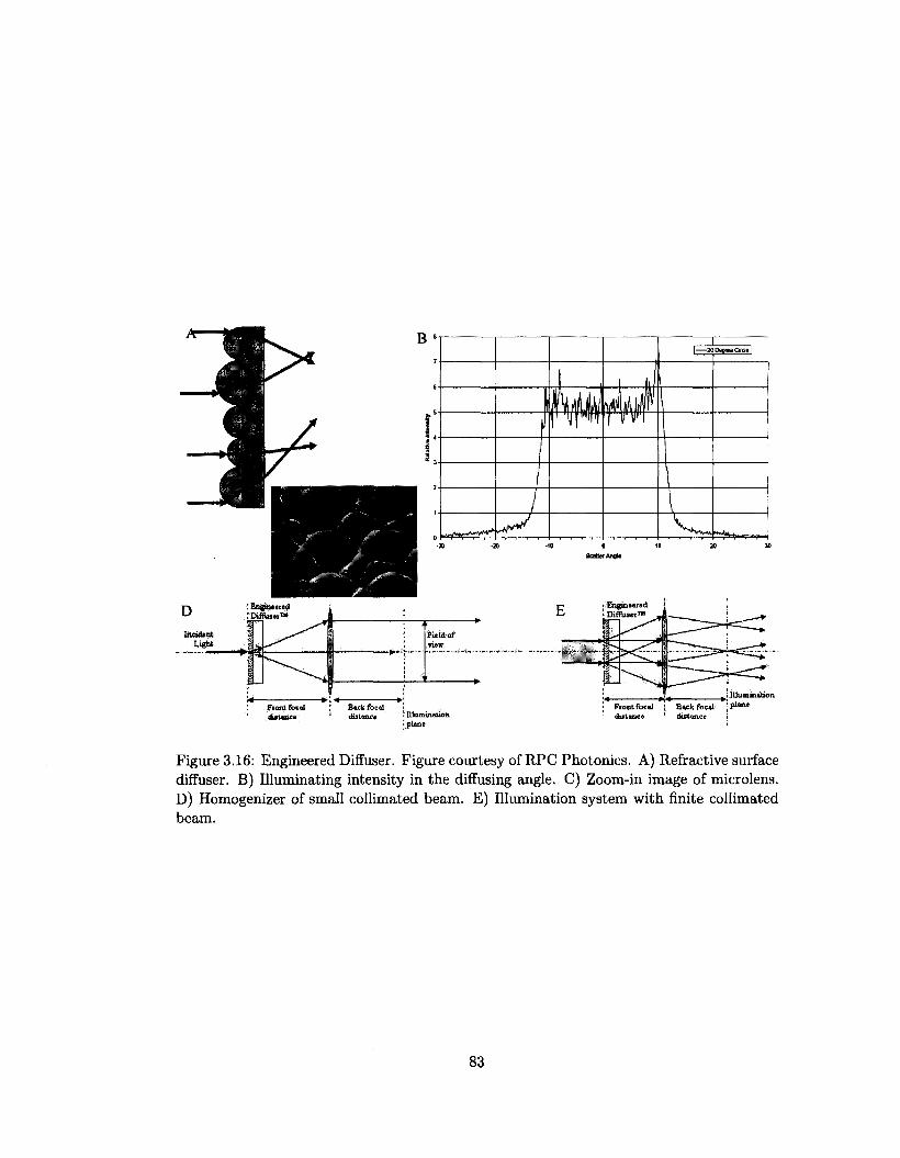
Figure 3.16: Engineered Diffuser. Figure courtesy of RPC Photonics. A) Refractive surface diffuser. B) Illuminating intensity in the diffusing angle. C) Zoom-in image of microlens. D) Homogenizer of small collimated beam. E) Illumination system with finite collimated beam.
83
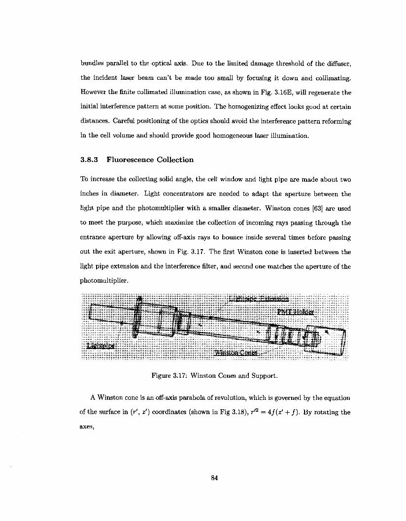
bundles parallel to the optical axis. Due to the limited damage threshold of the diffuser,
the incident laser beam can't be made too small by focusing it down and collimating.
However the finite collimated illumination case, as shown in Fig. 3.16E, will regenerate the
initial interference pattern at some position. The homogenizing effect looks good at certain
distances. Careful positioning of the optics should avoid the interference pattern reforming
in the cell volume and should provide good homogeneous laser illumination.
3.8.3 Fluorescence Collection
To increase the collecting solid angle, the cell window and light pipe are made about two
inches in diameter. Light concentrators are needed to adapt the aperture between the
light pipe and the photomultiplier with a smaller diameter. Winston cones [63] are used
to meet the purpose, which maximize the collection of incoming rays passing through the
entrance aperture by allowing off-axis rays to bounce inside several times before passing
out the exit aperture, shown in Fig. 3.17. The first Winston cone is inserted between the
light pipe extension and the interference filter, and second one matches the aperture of the
photomultiplier.
Figure 3.17: Winston Cones and Support.
A Winston cone is an off-axis parabola of revolution, which is governed by the equation
of the surface in (r', z') coordinates (shown in Fig 3.18), r'2 = 4f(z' + / ) . By rotating the
axes,
84
Figure 3.18: Schematic diagram of a Winston cone light concentrator. The entrance and exit apertures are of radius a and a', respectively. F is the focus of the upper parabola segments, and / is its focal length. The length of the cone is L. The origins and orientations of the focus-centered and symmetry axis-centered coordinate systems are shown also.
cos 0 — sin 6
sin 0 cos 0
a
0
the equation is expressed in (r, z) coordinates with r = y/x1 + z2, a and a' the radius of
entrance and exit apertures respectively,
(r cos 6 + z sin d)2 + a'r(l + sin 0)2 - 2a'z cos 0(1 + sin 0) - a'2(3 + sin 0)(1 + sin 6) = 0.
where 6 is the half of opening angle @c- a and a' will completely specify the geometry of
Winston cone by
9 G iE20 = 2sin-1 ( - J .
with the relation L = (a + a') cot 0 and / = a'(l 4- sin0).
In our case, the first cone has the radius of entrance aperture a = 2" and exit aperture
a' = 1.8", leading to a curve length of L = 0.92"; the second Winston cone has a = 1.8"
and a' = 1", leading to a curve length of L = 2.095", shown in Fig. 3.19. Both are made
85
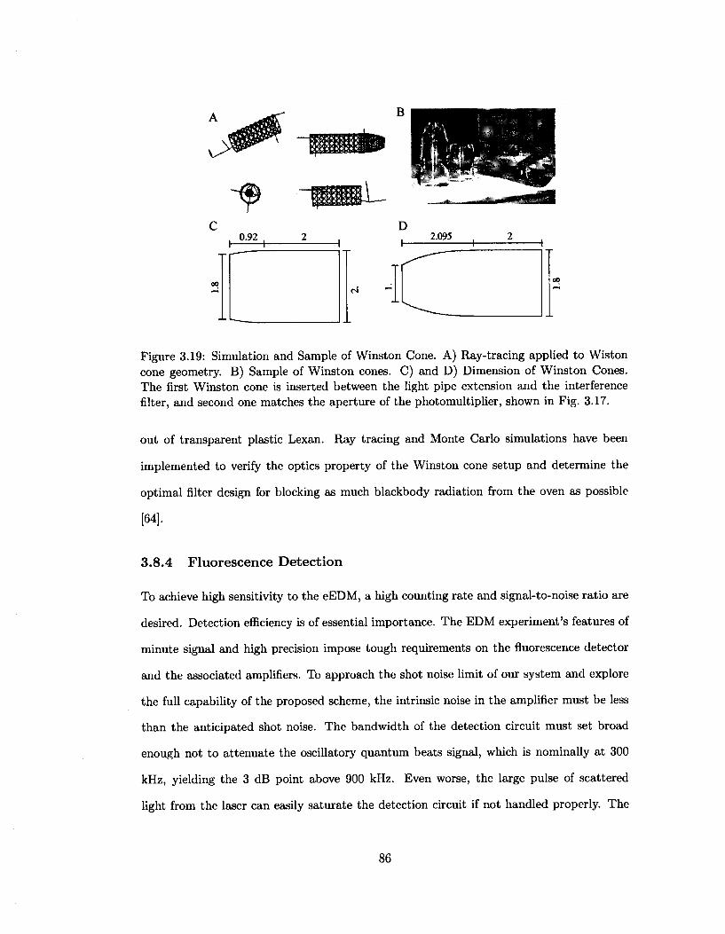
Figure 3.19: Simulation and Sample of Winston Cone. A) Ray-tracing applied to Wiston cone geometry. B) Sample of Winston cones. C) and D) Dimension of Winston Cones. The first Winston cone is inserted between the light pipe extension and the interference filter, and second one matches the aperture of the photomultiplier, shown in Fig. 3.17.
out of transparent plastic Lexan. Ray tracing and Monte Carlo simulations have been
implemented to verify the optics property of the Winston cone setup and determine the
optimal filter design for blocking as much blackbody radiation from the oven as possible
[64].
3.8.4 Fluorescence Detection
To achieve high sensitivity to the eEDM, a high counting rate and signal-to-noise ratio are
desired. Detection efficiency is of essential importance. The EDM experiment's features of
minute signal and high precision impose tough requirements on the fluorescence detector
and the associated amplifiers. To approach the shot noise limit of our system and explore
the full capability of the proposed scheme, the intrinsic noise in the amplifier must be less
than the anticipated shot noise. The bandwidth of the detection circuit must set broad
enough not to attenuate the oscillatory quantum beats signal, which is nominally at 300
kHz, yielding the 3 dB point above 900 kHz. Even worse, the large pulse of scattered
light from the laser can easily saturate the detection circuit if not handled properly. The
86
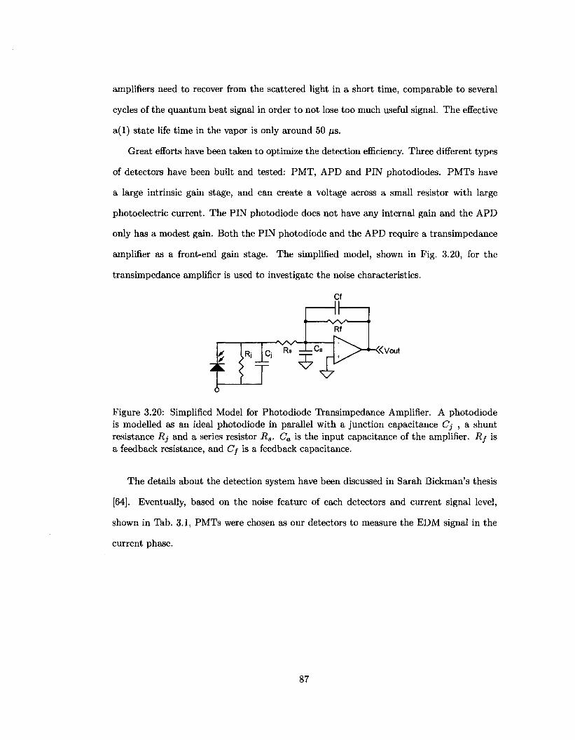
amplifiers need to recover from the scattered light in a short time, comparable to several
cycles of the quantum beat signal in order to not lose too much useful signal. The effective
a(l) state life time in the vapor is only around 50 /is.
Great efforts have been taken to optimize the detection efficiency. Three different types
of detectors have been built and tested: PMT, APD and PIN photodiodes. PMTs have
a large intrinsic gain stage, and can create a voltage across a small resistor with large
photoelectric current. The PIN photodiode does not have any internal gain and the APD
only has a modest gain. Both the PIN photodiode and the APD require a transimpedance
amplifier as a front-end gain stage. The simplified model, shown in Fig. 3.20, for the
transimpedance amplifier is used to investigate the noise characteristics.
Cf
t -"s/V 1
Rs
Rf
^ 7 #
«Vout
Figure 3.20: Simplified Model for Photodiode Transimpedance Amplifier. A photodiode is modelled as an ideal photodiode in parallel with a junction capacitance Cj , a shunt resistance Rj and a series resistor Rs. Ca is the input capacitance of the amplifier. Rf is a feedback resistance, and Cf is a feedback capacitance.
The details about the detection system have been discussed in Sarah Bickman's thesis
[64]. Eventually, based on the noise feature of each detectors and current signal level,
shown in Tab. 3.1, PMTs were chosen as our detectors to measure the EDM signal in the
current phase.
87
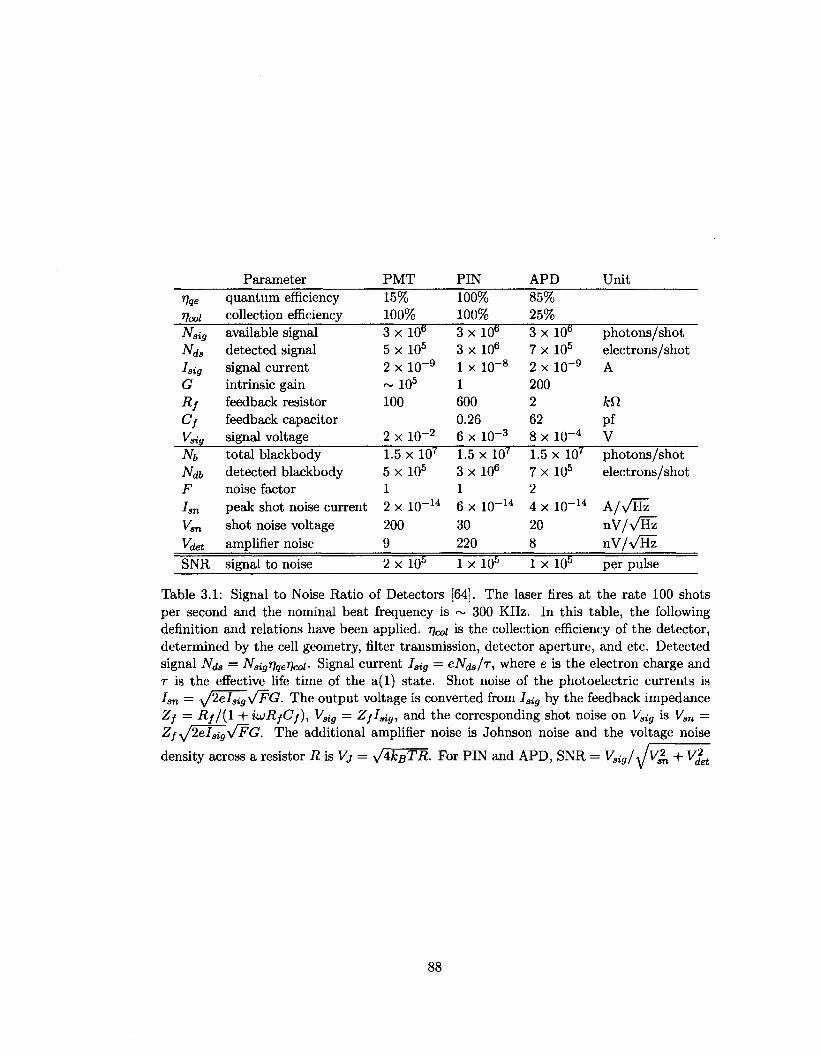
Parameter PMT PIN APD Unit Vqe
Vcol
•LVsig
Nda
lsig G Rf
Cf *sig
Nb
F
*-sn
van Vdet
SNR
quantum efficiency collection efficiency available signal detected signal signal current intrinsic gain feedback resistor feedback capacitor signal voltage total blackbody detected blackbody noise factor peak shot noise current shot noise voltage amplifier noise
signal to noise
15% 100% 3 x 10° 5 x l 0 5
2 x 10~9
~ 1 0 5
100
2 x 10~2
1.5 x 10' 5 x 10⁵
1 2 x 10~14
200 9
2 x 10⁵
100% 100% 3 x 10B
3 x l 0 6
1 x 10~8
1 600 0.26 6 x 10⁻³
1.5 x 10' 3 x 10⁶
1 6 x 10-14
30 220
1 x 10⁵
85% 25% 3 x 10° 7 x l 0 5
2 x 10~9
200 2 62 8 x 10⁻⁴
1.5 x 10'' 7 x 10⁵
2 4 x 10~14
20 8
1 xlO 5
photons/shot electrons/shot A
ktt pf V photons/shot electrons/shot
A/VHi nV/\/Hz
per pulse
Table 3.1: Signal to Noise Ratio of Detectors [64]. The laser fires at the rate 100 shots per second and the nominal beat frequency is ~ 300 KHz. In this table, the following definition and relations have been applied, rjcoi is the collection efficiency of the detector, determined by the cell geometry, filter transmission, detector aperture, and etc. Detected signal Nd3 — • sig^ge'Jco/- Signal current I gig = eA^s/r, where e is the electron charge and r is the effective life time of the a(l) state. Shot noise of the photoelectric currents is I an — y/2eIsig>/~FG. The output voltage is converted from Isig by the feedback impedance Zf = Rf/(l + iuRfCf), Vsig = ZfISig, and the corresponding shot noise on VSig is Vgn = Zf y/2eISig y/FG. The additional amplifier noise is Johnson noise and the voltage noise
density across a resistor R is Vj = y/4kBTR. For PIN and APD, SNR = Vsig/Jvs2n + V^t
88
Chapter 4
Molecular State Preparation
We have demonstrated the ability to manipulate the internal molecular state to produce the
desired states for our EDM experiment, using microwave excitation. Efforts were carried
out to optimize the state excitation efficiency. We performed various experiments to con
firm our understanding of molecular state evolution dynamics in a variety of experimental
configurations.
In this chapter, the details of molecular state preparation scheme using microwaves
will be discussed. Although our previous attempt using RF excitation were unsuccessful
(see Section 4.1), the microwave excitation scheme provides a convincing demonstration
of our ability to populate the desired molecular states (see Section 4.2). An adiabatic
following scheme has been implemented to optimize the efficiency of population transfer
(see Section 4.3). The experimental results from various configurations and parameter
regimes will be compared and discussed.
4.1 Previous Attempts using RF Excitation
The spectral width of pulsed laser and optical Doppler width are too broad to resolve
the $7-doublet levels. Moreover, in the presence of the external electric field 8, the e and
/ components of the fi-doublet levels with M ^ 0 are mixed. Both components will
89
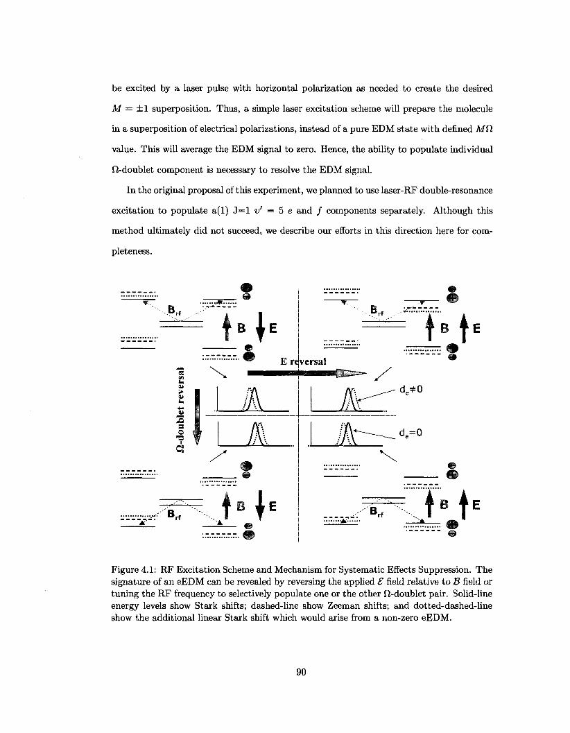
be excited by a laser pulse with horizontal polarization as needed to create the desired
M = ±1 superposition. Thus, a simple laser excitation scheme will prepare the molecule
in a superposition of electrical polarizations, instead of a pure EDM state with defined Mft
value. This will average the EDM signal to zero. Hence, the ability to populate individual
fi-doublet component is necessary to resolve the EDM signal.
In the original proposal of this experiment, we planned to use laser-RF double-resonance
excitation to populate a(l) J = l v' = 5 e and / components separately. Although this
method ultimately did not succeed, we describe our efforts in this direction here for com
pleteness.
.B,
> at
« PMM(
A s o -a G
Br
4 B 1
E reversal
4 B I . — • . • dfitili
m?
B rf
'•••.... Brt _,.-•«
t i"i A D T
d =*0
d = 0
f B t
Figure 4.1: RF Excitation Scheme and Mechanism for Systematic Effects Suppression. The signature of an eEDM can be revealed by reversing the applied £ field relative to B field or tuning the RF frequency to selectively populate one or the other fi-doublet pair. Solid-line energy levels show Stark shifts; dashed-line show Zeeman shifts; and dotted-dashed-line show the additional linear Stark shift which would arise from a non-zero eEDM.
90
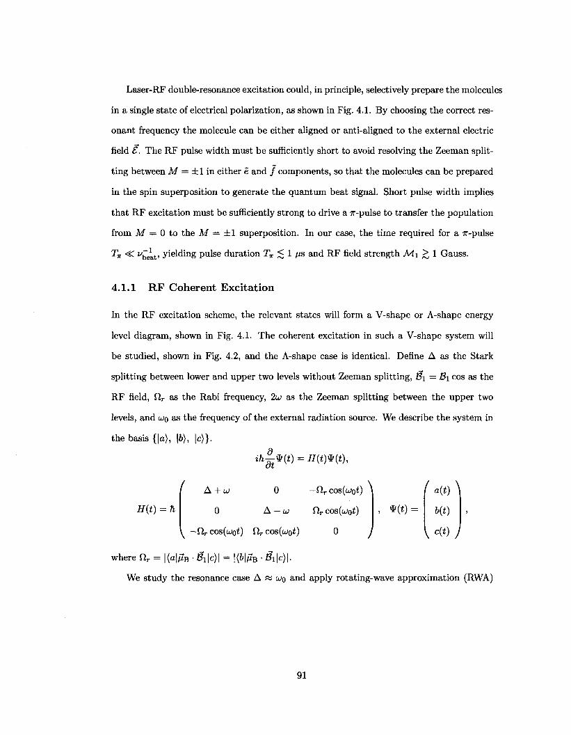
Laser-RF double-resonance excitation could, in principle, selectively prepare the molecules
in a single state of electrical polarization, as shown in Fig. 4.1. By choosing the correct res
onant frequency the molecule can be either aligned or anti-aligned to the external electric
field £. The RF pulse width must be sufficiently short to avoid resolving the Zeeman split
ting between M = ±1 in either e and / components, so that the molecules can be prepared
in the spin superposition to generate the quantum beat signal. Short pulse width implies
that RF excitation must be sufficiently strong to drive a 7r-pulse to transfer the population
from M = 0 to the M = ±1 superposition. In our case, the time required for a 7r-pulse
T„- <C "beati y i e ^ m § pulse duration Tw < 1 fis and RF field strength Mi > 1 Gauss.
4.1.1 RF Coherent Excitation
In the RF excitation scheme, the relevant states will form a V-shape or A-shape energy
level diagram, shown in Fig. 4.1. The coherent excitation in such a V-shape system will
be studied, shown in Fig. 4.2, and the A-shape case is identical. Define A as the Stark
splitting between lower and upper two levels without Zeeman splitting, B\ = B\ cos as the
RF field, fir as the Rabi frequency, 2UJ as the Zeeman splitting between the upper two
levels, and U>Q as the frequency of the external radiation source. We describe the system in
the basis {\a), |fc), |c)}.
d i / l -*( i) = HW(t),
(
H(t)
0
A - o ;
cos(u>ot)
—fir cos(o;oi)
Clr cos(u;o£)
0 )
, *(*) =
' a(t) ^
b(t)
y, c(t) j
A + w
0
1r cos(woi)
where ftr = \{a\pB • #i|c)| = \{b\jls • B\\c)\.
We study the resonance case A « CJQ and apply rotating-wave approximation (RWA)
91
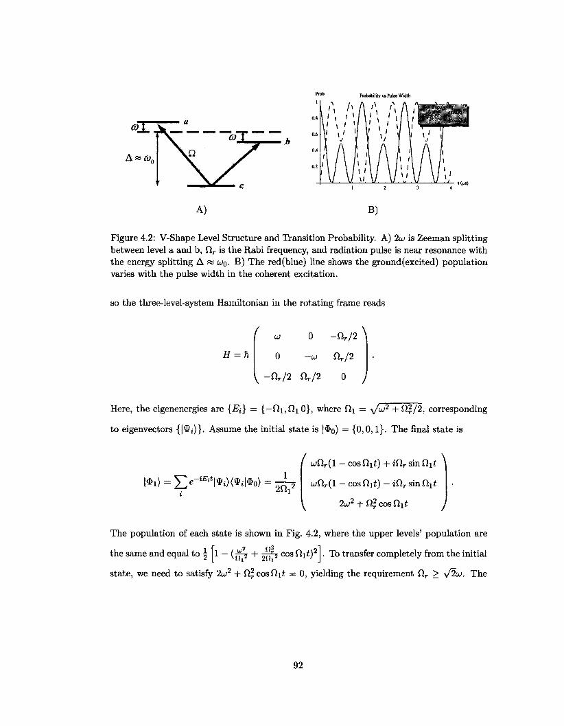
Probability vs Pulse Width
A«G)t
A)
Population CKCiled
B)
Figure 4.2: V-Shape Level Structure and Transition Probability. A) 2u is Zeeman splitting between level a and b, flr is the Rabi frequency, and radiation pulse is near resonance with the energy splitting A « UQ. B) The red(blue) line shows the ground(excited) population varies with the pulse width in the coherent excitation.
so the three-level-system Hamiltonian in the rotating frame reads
H = h
u o -nr/2
0 -u flr/2
\ -flr/2 flr/2 0 J
Here, the eigenenergies are {Ei} = {—fli,fliO}, where fli = \Ju)2 + fl2/2, corresponding
to eigenvectors {!*»)}. Assume the initial state is |$o) = {0,0,1}. The final state is
l*l> = £« _ ^W(*i l*0> = ^
ujflr(1 - cos flit) + iflr sin flit
ujflr(l — cosQii) — iflr sin flit
2u2 + fl2. cos flit
The population of each state is shown in Fig. 4.2, where the upper levels' population are
the same and equal to \ 1 — (jy-j + 5^% cos Slit)2 . To transfer completely from the initial
state, we need to satisfy 2UJ2 + fl2 cos flit = 0, yielding the requirement flr > y/2to. The
92
complete population transfer occurs at
where k = 0,1,2,. . . . Evidently, this reduces to the ordinary n pulse condition, 7r/fii, for
the degenerate case when u = 0. If the -K pulse condition holds, the final state ends in
{^Wm=SJ)t 2 ^ E M o} = { £ , ^ , 0}, where * = arccos ^ . If the size of
Q.r is comparable to -\/2w, the final state will end up in {l/-\/2,1/V^, 0}.
In this RF excitation scheme, the RF pulse drives the Ml transition between M=0 and
M = ±1 states. The typical values in our experimental conditions are Qr ~ 1 MHz and
u ~ 0.15 MHz, leading to the corresponding pulse width 0.36 /is, 1.03 fis, 1.74 /xs . . . The
typical RF pulse width is chosen to be around 1 /J,S, so that it is shorter than the beat
period to avoid inducing different initial beat phases during excitation and washing out
the beat contrast.
4.1.2 R F Experimental Setup
The requirement on a RF experimental setup is that we should drive a RF transition, with
pulse with width < 3 /is, and a frequency ranging from 20 MHz to 70 MHz, and switching
between two frequencies 11.2 MHz apart every other laser shot. The setup should sustain
700°C temperature and fit inside the limited space between the oven and vapor cell, without
putting any magnetic components close to the vacuum chamber.
We constructed a RF system that could deliver RF pulses with sufficient magnetic field
to drive the Ml transition, and switch between frequencies separated by An = 11.2 MHz
to access both fi-doublet levels of PbO a(l) 3 S + . The fast switching feature, enabled by
electromechanical relays, helps to eliminate various sources of systematic error by using
the O-doublet as an internal co-magnetometer.
Dimensional constraints in the current experimental setup forced us to implement the
system using single Helmholtz coils around the vapor cell braced by ceramic supports, and
2«7r ± arccos ( — — j -
93
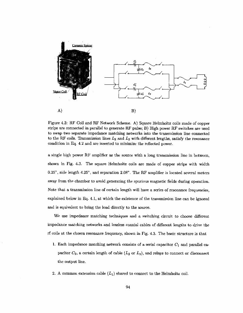
A) B)
Figure 4.3: RF Coil and RF Network Scheme. A) Square Helmholtz coils made of copper strips are connected in parallel to generate RF pulse; B) High power RF switches are used to swap two separate impedance matching networks into the transmission line connected to the RF coils. Transmission lines Li and L3 with different lengths, satisfy the resonance condition in Eq. 4.2 and are inserted to minimize the reflected power.
a single high power RF amplifier as the source with a long transmission line in between,
shown in Fig. 4.3. The square Helmholtz coils are made of copper strips with width
0.25", side length 4.25", and separation 2.08". The RF amplifier is located several meters
away from the chamber to avoid generating the spurious magnetic fields during operation.
Note that a transmission line of certain length will have a series of resonance frequencies,
explained below in Eq. 4.1, at which the existence of the transmission line can be ignored
and is equivalent to bring the load directly to the source.
We use impedance matching techniques and a switching circuit to choose different
impedance matching networks and lossless coaxial cables of different lengths to drive the
rf coils at the chosen resonance frequency, shown in Fig. 4.3. The basic structure is that
1. Each impedance matching network consists of a serial capacitor C\ and parallel ca
pacitor C2, a certain length of cable (L2 or £3), and relays to connect or disconnect
the output line.
2. A common extension cable {L\) shared to connect to the Helmholtz coil.
94

3. The electromechanical relays.
A single-turn square Helmholtz coil is connected parallel to reduce inductance, yield
ing a self inductance 0.25 /iH and capacitance 24.7 pF. Low-loss semi-rigid coaxial cables
are from Tim-Co (Catalog No. L14C), impedance 50 ± 0.5 fi, outer diameter 0.141".
Electromechanical relays switch between the two impedance-matched networks, with each
network working with typical values of C\ ~15 pF, C% ~60 pF for 33.6 MHz, or C\ ~8pF,
Ci ~25 pF for 44.8 MHz, etc. These capacitors are variable mica compression trimmers
from Arco Electronics. The electromechanical relays are Radiall RF Coaxial SPDT switch
R570313100, with insertion Loss < 0.20 dB. The switches and impedance matching net
works are mounted on double-sided copper clad and enclosed in a 5" x 6" x 9" aluminum
box. The enclosure and the copper clad are grounded to the RF cable ground for better
shielding.
Gdz V(z + clz) Zo
dz '-in -(
Figure 4.4: Transmission Line Model. Left: Network model is used to derive the telegraph equation for transmission line. Here R is a series resistance per unit length, L series inductance per unit length , G shunt conductance per unit length, and C shunt capacitance per unit length. Right: Load Z\ is connected to the transmission line with characteristic impedance Zo, length I.
To explain how this system works, I will give a brief description of transmission line
theory. The transmission line, capable of guiding TEM waves, can be modeled as small
cascaded circuit elements, shown in Fig. 4.4, where R is a series resistance per unit length,
L series inductance per unit length , G shunt conductance per unit length, and C shunt
capacitance per unit length. The voltage and current in the transmission line satisfy the
95
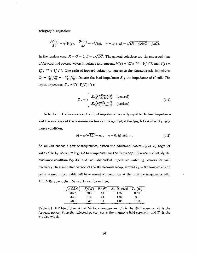
telegraph equation:
In the lossless case, R = G = 0, j3 = ujy/LC. The general solutions are the superpositions
of forward and reverse waves in voltage and current, V(z) = V^+e-7* + V0~e72, and I(z) =
Jo"e-7Z + I^e1*' • The ratio of forward voltage to current is the characteristic impedance
Zo = ^o+Ao" = ~VQ~/IQ- Denote the load impedance ZL, the impedance of rf coil. The
input impedance Z-m = V(-l)/I(-l) is
Z0zSt?ot™tt- (general) Zin={ Uz°+*Ltanh7r « ; ( 4 1 )
Note that in the lossless case, the input impedance is exactly equal to the load impedance
and the existence of the transmission line can be ignored, if the length 1 satisfies the reso
nance condition,
Pl = uly/W = nn, n = 0 , ± l , ± 2 , . . . (4.2)
So we can choose a pair of frequencies, attach the additional cables Li or L% together
with cable L\, shown in Fig. 4.3 to compensate for the frequency difference and satisfy the
resonance condition Eq. 4.2, and use independent impedance matching network for each
frequency. In a simplified version of the RF network setup, around L\ = 30' long extension
cable is used. Such cable will have resonance condition at the multiple frequencies with
11.2 MHz apart, then Li and L3 can be omitted.
/rf (MHz) P/(W) Pr(W) Brf (Gauss) T« (JJS) 33.6 603 44 1.27 0.87 44.8 614 44 1.37 0.8 56.0 647 81 l_m 1.07
Table 4.1: RF Field Strength at Various Frequencies. /rf is the RF frequency, Pj is the forward power, Pr is the reflected power, f?rf is the magnetic field strength, and Tn is the 7r pulse width.
96
We constructed a system capable of generating a RF field sufficiently strong to drive
the RF transition in around 1 /JS, at two frequencies separated by An = 11.2 MHz. The
results are listed in Tab. 4.1. The RF field is measured using a calibrated pickup coil.
The pickup coil is 1/8" diameter pickup loop using 32-gauge magnet wire, with 50 Q. SMT
resistor in serial and extended using semi-rigid cable. The pickup coil's intrinsic resonance
frequency is 206MHz, far beyond our working frequency, hence has flat frequency response
at RF frequency range. The forward power Pf and the reflected power Pr are read from
the panel of the RF amplifier. The reflected powers are due to the imperfect tuning of
the impedance matching networks. The reflected power is small enough that we can still
deliver a sufficiently high power RF pulse.
4.1.3 RF Transition Efficiency
We encountered great difficulty to achieving high RF-transition efficiency in exciting the
desired a(l) J = 1, M = ±1 spin superpositions. The reason for this difficulty remains elu
sive and possible explanations will be discussed later. In the meantime, we demonstrated
de-excitation of the M = ±1 superposition states efficiently. We applied a static elec
tric field and drove laser excitation with horizontal polarization to prepare the molecules
in the M = ±1 superposition states, subsequently applied the horizontal RF pulse, and
monitored the Zeeman quantum beats. The experimental result was in qualitatively rea
sonable agreement with the expectation: nearly-complete disappearance of beats with the
transition to an M = 0 state at the correct frequencies and pulse width Tff.
The typical method to carry out the experiment was to fix the RF frequency, and vary
the voltage applied on the electrodes, thus changing the Stark energy splitting, to cross
through the resonance frequency. Fig. 4.5 shows the beat dips as the electrode voltage
scans. As the molecules populate both M = ±1 states of e and / components by the
horizontal polarized laser in the presence of the electric field, the first beat amplitude dip
will occur when the energy splitting between M = ±1 e and M = 0 / components matches
the RF frequency, and second dip occurs when the energy splitting between M = ±1 e and
97
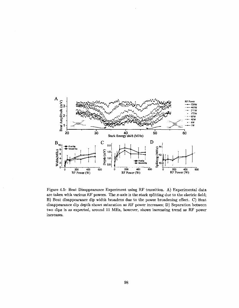
« . . . , . L_J , , . , . , </> i; , , , , _ _ , 0 200 400 600 0 200 400 600 0 200 400 600
RF Power (W) RF Power (W) RF Power (W)
Figure 4.5: Beat Disappearance Experiment using RF transition. A) Experimental data are taken with various RF powers. The x-axis is the stark splitting due to the electric field; B) Beat disappearance dip width broadens due to the power broadening effect. C) Beat disappearance dip depth shows saturation as RF power increases; D) Separation between two dips is as expected, around 11 MHz, however, shows increasing trend as RF power increases.
98
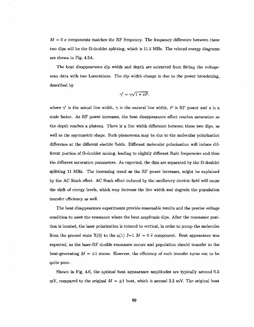
M = 0 e components matches the RF frequency. The frequency difference between these
two dips will be the ft-doublet splitting, which is 11.2 MHz. The related energy diagrams
are shown in Fig. 4.5A.
The beat disappearance dip width and depth are extracted from fitting the voltage-
scan data with two Lorentzians. The dip width change is due to the power broadening,
described by
y = 7V1 + SP,
where 7' is the actual line width, 7 is the natural line width, P is RF power and s is a
scale factor. As RF power increases, the beat disappearance effect reaches saturation as
the depth reaches a plateau. There is a line width difference between these two dips, as
well as the asymmetric shape. Such phenomena may be due to the molecular polarization
difference at the different electric fields. Different molecular polarization will induce dif
ferent portion of f2-doublet mixing, leading to slightly different Rabi frequencies and thus
the different saturation parameters. As expected, the dips are separated by the fi-doublet
splitting 11 MHz. The increasing trend as the RF power increases, might be explained
by the AC Stark effect. AC Stark effect induced by the oscillatory electric field will cause
the shift of energy levels, which may increase the line width and degrade the population
transfer efficiency as well.
The beat disappearance experiments provide reasonable results and the precise voltage
condition to meet the resonance where the beat amplitude dips. After the resonance posi
tion is located, the laser polarization is rotated to vertical, in order to pump the molecules
from the ground state X(0) to the a(l) J = l M = 0 e component. Beat appearance was
expected, as the laser-RF double resonance occurs and population should transfer to the
beat-generating M = ±1 states. However, the efficiency of such transfer turns out to be
quite poor.
Shown in Fig. 4.6, the optimal beat appearance amplitudes are typically around 0.5
mV, compared to the original M = ±1 beat, which is around 2.5 mV. The original beat
99
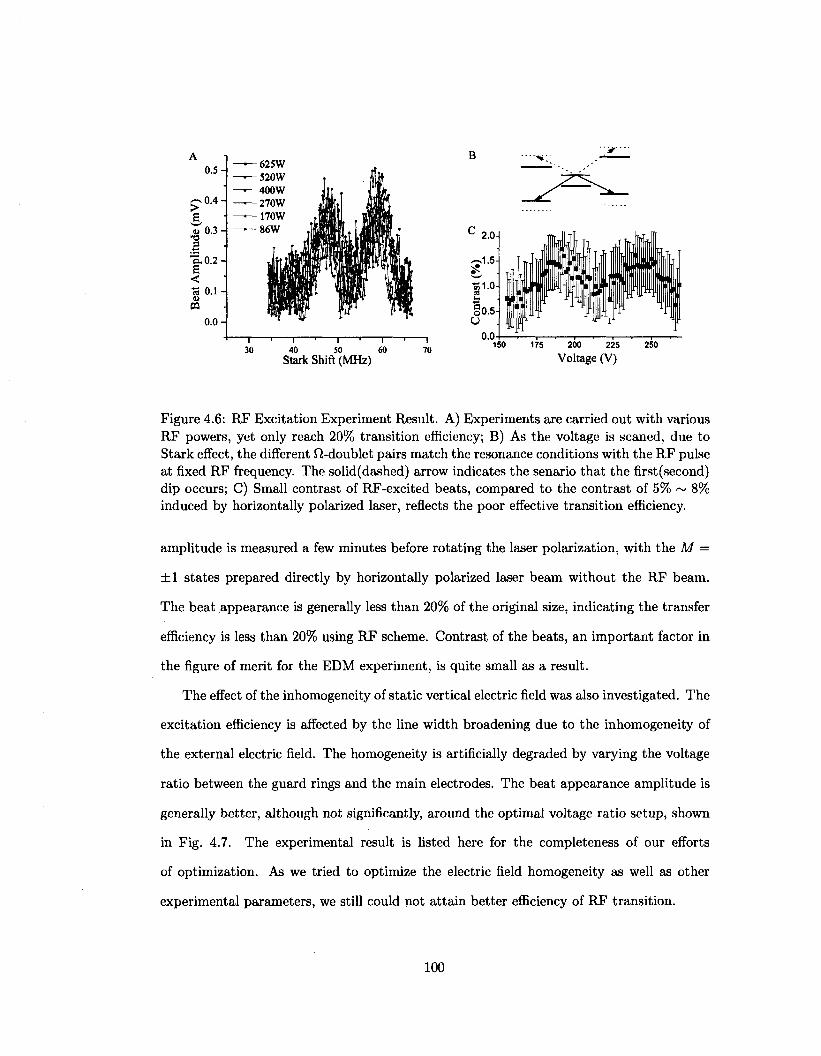
Figure 4.6: RF Excitation Experiment Result. A) Experiments are carried out with various RF powers, yet only reach 20% transition efficiency; B) As the voltage is scaned, due to Stark effect, the different ^-doublet pairs match the resonance conditions with the RF pulse at fixed RF frequency. The solid(dashed) arrow indicates the senario that the first (second) dip occurs; C) Small contrast of RF-excited beats, compared to the contrast of 5% ~ 8% induced by horizontally polarized laser, reflects the poor effective transition efficiency.
amplitude is measured a few minutes before rotating the laser polarization, with the M =
±1 states prepared directly by horizontally polarized laser beam without the RF beam.
The beat appearance is generally less than 20% of the original size, indicating the transfer
efficiency is less than 20% using RF scheme. Contrast of the beats, an important factor in
the figure of merit for the EDM experiment, is quite small as a result.
The effect of the inhomogeneity of static vertical electric field was also investigated. The
excitation efficiency is affected by the line width broadening due to the inhomogeneity of
the external electric field. The homogeneity is artificially degraded by varying the voltage
ratio between the guard rings and the main electrodes. The beat appearance amplitude is
generally better, although not significantly, around the optimal voltage ratio setup, shown
in Fig. 4.7. The experimental result is listed here for the completeness of our efforts
of optimization. As we tried to optimize the electric field homogeneity as well as other
experimental parameters, we still could not attain better efficiency of RF transition.
100
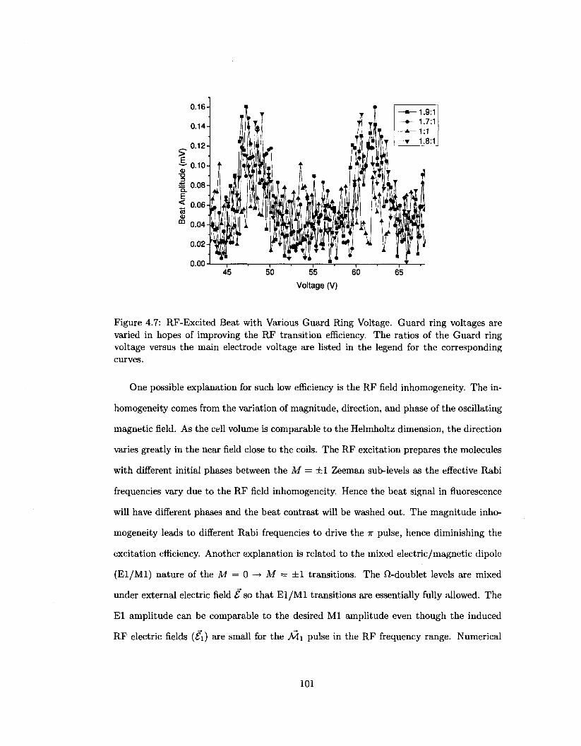
—I 1 1 1 1 1 ,—
45 50 55 60
Voltage (V)
Figure 4.7: RF-Excited Beat with Various Guard Ring Voltage. Guard ring voltages are varied in hopes of improving the RF transition efficiency. The ratios of the Guard ring voltage versus the main electrode voltage are listed in the legend for the corresponding curves.
One possible explanation for such low efficiency is the RF field inhomogeneity. The in-
homogeneity comes from the variation of magnitude, direction, and phase of the oscillating
magnetic field. As the cell volume is comparable to the Helmholtz dimension, the direction
varies greatly in the near field close to the coils. The RF excitation prepares the molecules
with different initial phases between the M = ±1 Zeeman sub-levels as the effective Rabi
frequencies vary due to the RF field inhomogeneity. Hence the beat signal in fluorescence
will have different phases and the beat contrast will be washed out. The magnitude inho
mogeneity leads to different Rabi frequencies to drive the 7r pulse, hence diminishing the
excitation efficiency. Another explanation is related to the mixed electric/magnetic dipole
(El/Ml) nature of the M = 0 —> M = ±1 transitions. The fi-doublet levels are mixed
under external electric field E so that E l /Ml transitions are essentially fully allowed. The
El amplitude can be comparable to the desired Ml amplitude even though the induced
RF electric fields (£i) are small for the M.\ pulse in the RF frequency range. Numerical
101
simulation of induced £\ shows it will mostly be along the vertical direction z due to the
rnetalic surface of the electrodes embedded in the cell. The El process will induce line
broadening mainly in higher order (AC Stark shifts from the component £i||.Mi).
In conclusion, we achieved little progress to improve the efficiency of the RF excitation
scheme after taking a lot of efforts. Eventually we gave up this direction and resorted to
new excitation scheme which will be discussed in the next section.
4.2 State Population Transfer using Microwave Excitaion
Although tremendous work has been done trying to improve the efficiency of the RF excita
tion scheme, we achieved little progress and eventually gave up this direction. However, the
microwave excitation scheme was proposed and implemented in the mean time. The first
trial was so appealing and convincing that we chose this scheme as the primary excitation
method.
The general description of microwave excitation is as following, shown in Fig. 4.8. A
pulsed laser at 571 nm excites PbO molecules from the X[J = 0+ , v=l] state to the
a(l)[J = 1~, M=0, v'=5] state. These are transferred to a coherent superposition of
M = ±1 levels in either the e or / component of the fi-doublet by a sequential Raman
transition at ~ 28.2 GHz using the a(l)[J=2, v'=5] intermediate state. The a(l)[J=l,
M = ±1 , v'=5>] molecules are detected by fluorescence at 548 nm that accompanies their
decay to X[v"=0].
4.2.1 a(l) 3=2 Rotational State
In order to explain the whole excitation procedure, it's necessary to give a complete de
scription of the relevant states. First we will study the level structure of a(l) J=2 under
the external static electromagnetic field, S = £z and B = Bz. The H-doublet splitting is
oc J(J+ l)Ajj for each J level respectively, so that fi-doublet splitting for J=2 will be three
times that of J = l level, equal to 3AJJ. The Lande factor depends on angular momentum
102
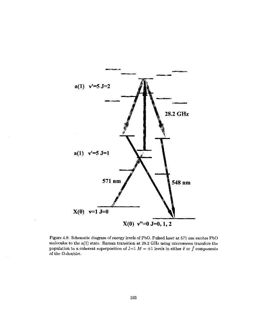
a(l) v'=5J=2
a(l) v'=5J=l
X(0) v=U=0
X(0) v"=0 J=0,1, 2
Figure 4.8: Schematic diagram of energy levels of PbO. Pulsed laser at 571 nm excites PbO molecules to the a(l) state. Raman transition at 28.2 GHz using microwaves transfers the population to a coherent superposition of J = l M = ±1 levels in either e or / components of the fl-doublet.
103
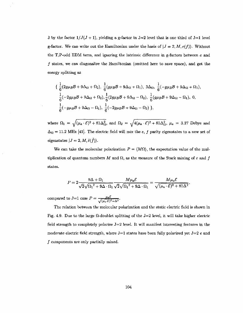
J by the factor 1/J{J + 1), yielding a g-factor in J=2 level that is one third of J = l level
g-factor. We can write out the Hamiltonian under the basis of \J = 2,M,e(f)). Without
the T,P-odd EDM term, and ignoring the intrinsic difference in g-factors between e and
/ states, we can diagonalize the Hamiltonian (omitted here to save space), and get the
energy splitting as
{^{2gnBB + 9An + ih), ~{gtiBB+ 9An + n1), 3A„, ^(-gtiBB + 9A„ + Hi),
-(-2gtXBB + 9An + n2),^(2gfxBB + 9An-n2), \(g»BB + 9AU - Qi), 0,
-{-giiBB + 9An - ni) , ^{-29liBB + 9AQ - il2) } ,
where fii = ^/(/J0 • £)2 + 81A£, and fi2 = ^/4(/ja • £)2 + 81A2>, /x„ = 3.27 Debye and
AJJ = 11.2 MHz [41]. The electric field will mix the e, / parity eigenstates to a new set of
eigenstates \J = 2,M, e(/)).
We can take the molecular polarization P = (Mil), the expectation value of the mul
tiplication of quantum numbers M and il, as the measure of the Stark mixing of e and /
states.
p = 2- 9 A + fii M^£ - M^e
' V2 v ^ i 2 + 9A • fii \ /2vtoi2 + 9A • fy v/(/ i a-£)2 + 81A2 '
compared to J = l case P = . ^a „
The relation between the molecular polarization and the static electric field is shown in
Fig. 4.9. Due to the large fi-doublet splitting of the J=2 level, it will take higher electric
field strength to completely polarize i—2 level. It will manifest interesting features in the
moderate electric field strength, where J = l states have been fully polarized yet J=2 e and
/ components are only partially mixed.
104
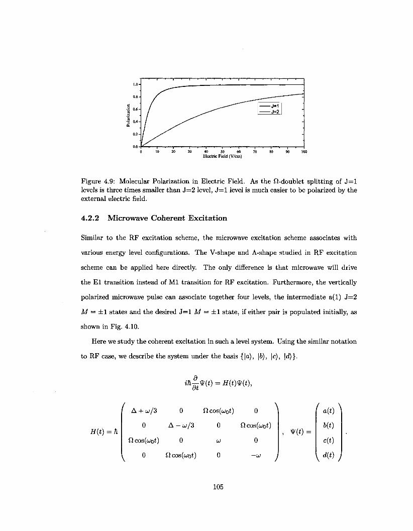
10 - I — ' — I — ' — I -4 0 5 0 6 0
Electric Field (V/cm)
Figure 4.9: Molecular Polarization in Electric Field. As the fi-doublet splitting of J = l levels is three times smaller than 3=2 level, J = l level is much easier to be polarized by the external electric field.
4.2.2 Microwave Coherent Excitation
Similar to the RF excitation scheme, the microwave excitation scheme associates with
various energy level configurations. The V-shape and A-shape studied in RF excitation
scheme can be applied here directly. The only difference is that microwave will drive
the El transition instead of Ml transition for RF excitation. Furthermore, the vertically
polarized microwave pulse can associate together four levels, the intermediate a(l) J=2
M = ±1 states and the desired J = l M = ±1 state, if either pair is populated initially, as
shown in Fig. 4.10.
Here we study the coherent excitation in such a level system. Using the similar notation
to RF case, we describe the system under the basis {\a), \b), \c), \d)}.
ih^m = H(w(t),
H(t) = h
A + w/3 0 Clcos(ujot) 0
0 A - w / 3 0 ficos(w0t)
ficos(o;o0 0 u; 0
0 ficos(a;o£) 0 —u
, * ( * ) =
/ a(t) ^
b(t)
c(t)
V d W J
105
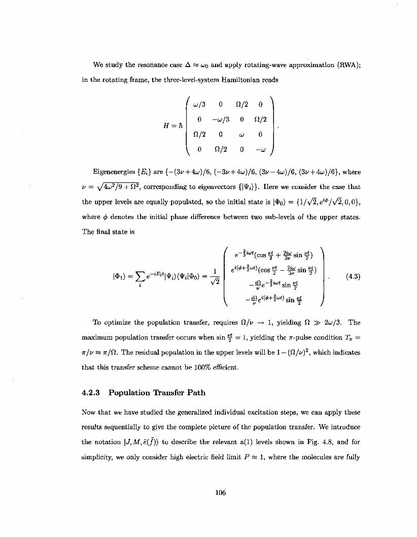
We study the resonance case A « u>o and apply rotating-wave approximation (RWA);
in the rotating frame, the three-level-system Hamiltonian reads
' u>/3 0 12/2 0 \
0 -w/3 0 n /2
n /2 0 a; 0
^ 0 fi/2 0 -u ,
Eigenenergies {£»} are {-(3i/ + 4w)/6, (-3i/ + 4w)/6, ( 3 I / - 4 J ) / 6 , (3^ + 4o;)/6}, where
/T = ft
1/ = v/4w2/9 + fi2, corresponding to eigenvectors {|*j)}. Here we consider the case that
the upper levels are equally populated, so the initial state is |$o) = {l/>/2,e'^/V^, 0,0},
where <f> denotes the initial phase difference between two sub-levels of the upper states.
The final state is
/ e - f ^ ( c o s f - l - ^ s i n f ) ^
l*i> = £ ' -iEiti * i> ( * i | *0> = V2
ei(<l>+3^)(cOS^ Zv s ing)
_ < a c - 3 iwt
sin vt
\ .^ e i(0+§u;t) s i n^
(4.3)
/
To optimize the population transfer, requires Q/u —> 1, yielding ft 3> 2OJ/3. The
maximum population transfer occurs when sin y = 1, yielding the 7r-pulse condition Tw =
7r/i/ « 7r/Q. The residual population in the upper levels will be 1 — (0,/v)2, which indicates
that this transfer scheme cannot be 100% efficient.
4.2.3 Population Transfer Path
Now that we have studied the generalized individual excitation steps, we can apply these
results sequentially to give the complete picture of the population transfer. We introduce
the notation \J, M, e(/)) to describe the relevant a(l) levels shown in Fig. 4.8, and for
simplicity, we only consider high electric field limit F « l , where the molecules are fully
106
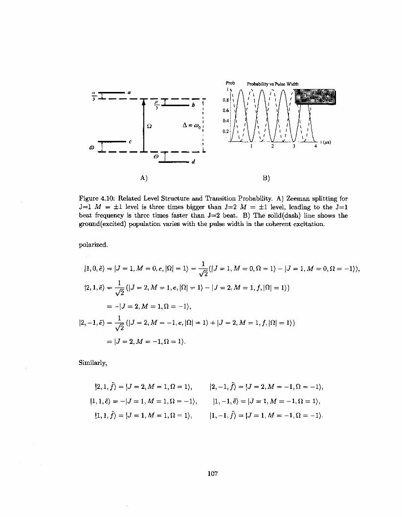
— I 3 ••*-
0 i
-X
Q
CO X
b i
A&con
Prob Probability vs Pulse Width
I ppcr
A) B)
Figure 4.10: Related Level Structure and Transition Probability. A) Zeeman splitting for J = l M = ±1 level is three times bigger than J=2 M = ±1 level, leading to the J = l beat frequency is three times faster than J=2 beat. B) The solid(dash) line shows the ground(excited) population varies with the pulse width in the coherent excitation.
polarized.
|l,0,e) = | J = 1,M = 0,e, \Q\ = 1) = -j,{\J = 1,M = 0,Q = 1) - \J = 1,M = 0,ft = - l ) ) , V2
|2,1, e) = -j= (| J = 2, M = 1, e, |0 | = 1) - | J = 2, M = 1, / , |0 | = 1))
= - | j = 2,Af = i , n = - i ) ,
| 2 , - l , e ) = - L (|J = 2,M = - l , e , |fl| = 1) + | J = 2,M = 1,/ , |fi| = 1))
= | j = 2,Af = - i , n = i>.
Similarly,
|2,1,/) = \J = %M = l,n = 1), 12,-1,/) = k = 2,M = -1 ,Q = -1 ) ,
| l , l ,e) = - | J = 1,M = l , n = -1 ) , | l , - l , e> = | J = 1,M = - 1 , 0 = 1),
|i,i,7> = |J = I , M = i,n = i), 11,-1,7) = \J = I,M = - i , n = - i ) .
107
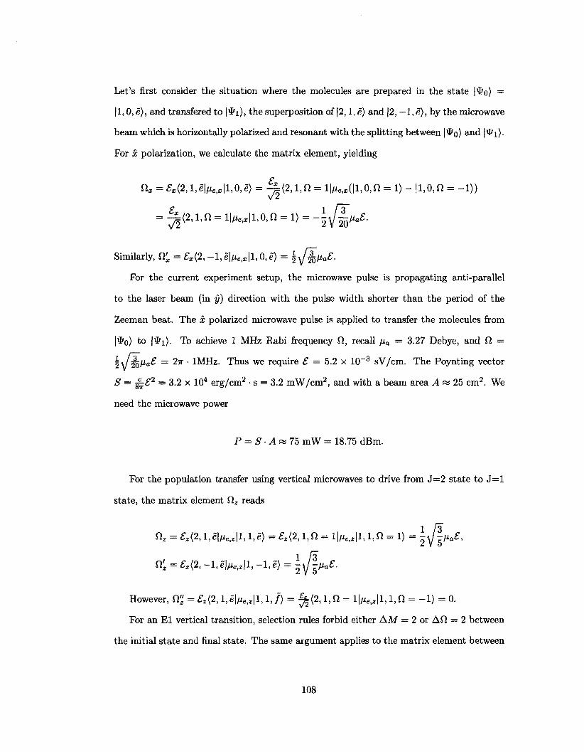
Let's first consider the situation where the molecules are prepared in the state |\I>o) =
|1,0, e), and transfered to |* i ) , the superposition of |2,1, e) and |2, — 1, e), by the microwave
beam which is horizontally polarized and resonant with the splitting between |\&o) and |\Pi).
For x polarization, we calculate the matrix element, yielding
nx = fx<2,i,c|/ie |i,o,g> = %(2,i,n = i|/*e^(|i,o,n = i) - |i,o,n = -i»
= ^(2,i,n = iKx|i,o,fi = i) = -\\J^a£.
Similarly, Sl'x = £x(2, -l,e|/ie>x | l ,0,e) = \J^^a£-
For the current experiment setup, the microwave pulse is propagating anti-parallel
to the laser beam (in y) direction with the pulse width shorter than the period of the
Zeeman beat. The x polarized microwave pulse is applied to transfer the molecules from
|\&o) to |* i ) . To achieve 1 MHz Rabi frequency fi, recall /ia = 3.27 Debye, and Q, —
lyW)^ = 27r ' 1MHz. Thus we require £ = 5.2 x 10~3 sV/cm. The Poynting vector
S = -g^£2 = 3.2 x 10⁴ erg/cm2 • s = 3.2 mW/cm2, and with a beam area A « 25 cm2. We
need the microwave power
P = S • A « 75 mW = 18.75 dBm.
For the population transfer using vertical microwaves to drive from J=2 state to J = l
state, the matrix element fi2 reads
n , = fa(2,l,c|/ie^|l , l ,e) = f , (2 , l , n = l | / ie, , | l , l ,n = l> = ^ | M « 5 ,
Sl'z = £z(2,~l,e\iie,z\l,-l,e) = y^a£.
However, {% = Ss{2, l,e|/ie,*|l, l,/> = ^ ( 2 , l , f i = l\iie,z\l,l,n = -1) = 0.
For an El vertical transition, selection rules forbid either AM = 2 or Afi — 2 between
the initial state and final state. The same argument applies to the matrix element between
108
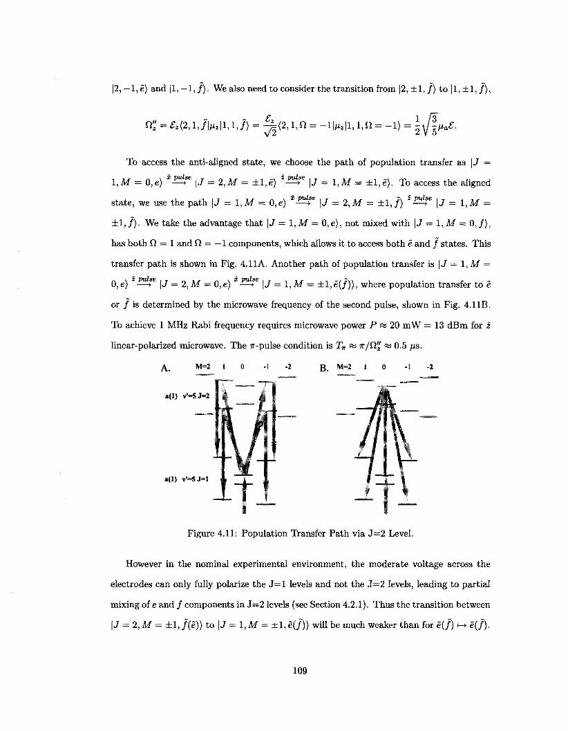
|2, —1, e) and |1, —1, / ) . We also need to consider the transition from |2, ±1, / ) to |1, ±1 , / ) ,
n;, = £,<2,i,/|A»*|i,i,/> = %<2,i,n = - i |^ | i , i ,n = -i> = iy | / i a f .
To access the anti-aligned state, we choose the path of population transfer as | J =
1,M = 0,e) *^e \J = 2,M = ±l,e) * ^ \J = 1,M = ±l,e). To access the aligned
state, we use the path \J = 1,M = 0,e) *^e \J = 2,M = ±1 , / ) * ^ e | J = 1,M =
±1 , / ) . We take the advantage that \J = \,M = 0,e), not mixed with \J = l,M = 0, / ) ,
has both $7 = 1 and il = — 1 components, which allows it to access both e and / states. This
transfer path is shown in Fig. 4.11A. Another path of population transfer is | J = 1, M —
0, e) —• |J = 2, M — 0,e) —• |J = 1,M — ±1,e(/)), where population transfer to e
or / is determined by the microwave frequency of the second pulse, shown in Fig. 4.11B.
To achieve 1 MHz Rabi frequency requires microwave power P RS 20 mW = 13 dBm for z
linear-polarized microwave. The 7r-pulse condition is Tv « TT/H" « 0.5 fis.
A. M=2 1 0 - 1 - 2 g_ M=2 1 0 - 1 - 2
a(l) v'=5J=2
a(l) v'=5J=l
Figure 4.11: Population Transfer Path via J=2 Level.
However in the nominal experimental environment, the moderate voltage across the
electrodes can only fully polarize the J = l levels and not the J—2 levels, leading to partial
mixing of e and / components in J=2 levels (see Section 4.2.1). Thus the transition between
\J = 2,M = ±1 , /(e)) to |J = 1,M = ±1 , e(/)) will be much weaker than for e{f) •-> e(/) .
109
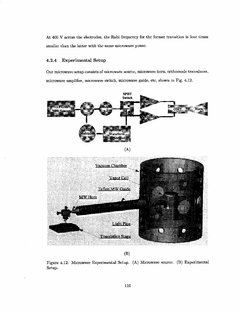
At 400 V across the electrodes, the Rabi frequency for the former transition is four times
smaller than the latter with the same microwave power.
4 .2 .4 E x p e r i m e n t a l S e t u p
Our microwave setup consists of microwave source, microwave horn, orthomode transducer,
microwave amplifier, microwave switch, microwave guide, etc, shown in Fig. 4.12.
SPDT Switch
13.1 (III/ M\\ Source
— Mixer «•»•
I MIK
Multiplier xN
Doiihlcr x2 "
rfnnM.jAmplifier
• • & ' • '
"""" -Amplifier
I
Waveform
OMT
J Horn
(A)
Vacuum Chamber
(B)
Figure 4.12: Microwave Experimental Setup. (A) Microwave source. (B) Experimental Setup.
110
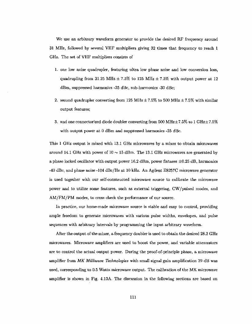
We use an arbitrary waveform generator to provide the desired RF frequency around
31 MHz, followed by several VHF multipliers giving 32 times that frequency to reach 1
GHz. The set of VHF multipliers consists of
1. one low noise quadrupler, featuring ultra low phase noise and low conversion loss,
quadrupling from 31.25 MHz ± 7.5% to 125 MHz ± 7.5% with output power at 12
dBm, suppressed harmonics -25 dBc, sub-harmonics -30 dBc;
2. second quadrupler converting from 125 MHz ± 7.5% to 500 MHz ± 7.5% with similar
output features;
3. and one connectorized diode doubler converting from 500 MHz±7.5% to 1 GHz±7.5%
with output power at 0 dBm and suppressed harmonics -25 dBc.
This 1 GHz output is mixed with 13.1 GHz microwaves by a mixer to obtain microwaves
around 14.1 GHz with power of 10 ~ 15 dBm. The 13.1 GHz microwaves are generated by
a phase locked oscillator with output power 16.2 dBm, power flatness ±0.25 dB, harmonics
-40 dBc, and phase noise -104 dBc/Hz at 10 kHz. An Agilent E8257C microwave generator
is used together with our self-constructed microwave source to calibrate the microwave
power and to utilize some features, such as external triggering, CW/pulsed modes, and
AM/FM/PM modes, to cross check the performance of our source.
In practice, our home-made microwave source is stable and easy to control, providing
ample freedom to generate microwaves with various pulse widths, envelopes, and pulse
sequences with arbitrary intervals by programming the input arbitrary waveform.
After the output of the mixer, a frequency doubler is used to obtain the desired 28.2 GHz
microwaves. Microwave amplifiers are used to boost the power, and variable attenuators
are to control the actual output power. During the proof-of-principle phase, a microwave
amplifier from MK Milliwave Technologies with small signal gain amplification 29 dB was
used, corresponding to 0.5 Watts microwave output. The calibration of the MK microwave
amplifier is shown in Fig. 4.13A. The discussion in the following sections are based on
111
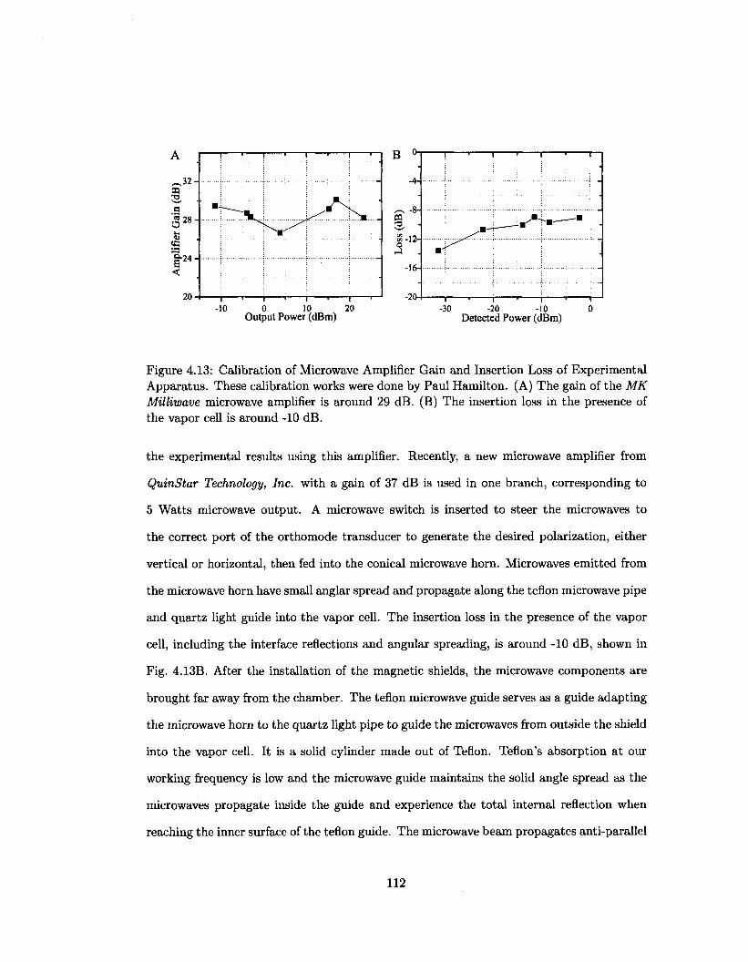
.32-05 7>
^ 28
&
t 2 4
< 20
-10
: t^JUri-..:
0 10 20 Output Power (dBm)
B »
-4-
0) 2-w -12-o *4 -164
-20- - 1 • 1 ' 1 • r--30 -20 -10 0
Detected Power (dBm)
Figure 4.13: Calibration of Microwave Amplifier Gain and Insertion Loss of Experimental Apparatus. These calibration works were done by Paul Hamilton. (A) The gain of the MK Milliwave microwave amplifier is around 29 dB. (B) The insertion loss in the presence of the vapor cell is around -10 dB.
the experimental results using this amplifier. Recently, a new microwave amplifier from
QuinStar Technology, Inc. with a gain of 37 dB is used in one branch, corresponding to
5 Watts microwave output. A microwave switch is inserted to steer the microwaves to
the correct port of the orthomode transducer to generate the desired polarization, either
vertical or horizontal, then fed into the conical microwave horn. Microwaves emitted from
the microwave horn have small anglar spread and propagate along the teflon microwave pipe
and quartz light guide into the vapor cell. The insertion loss in the presence of the vapor
cell, including the interface reflections and angular spreading, is around -10 dB, shown in
Fig. 4.13B. After the installation of the magnetic shields, the microwave components are
brought far away from the chamber. The teflon microwave guide serves as a guide adapting
the microwave horn to the quartz light pipe to guide the microwaves from outside the shield
into the vapor cell. It is a solid cylinder made out of Teflon. Teflon's absorption at our
working frequency is low and the microwave guide maintains the solid angle spread as the
microwaves propagate inside the guide and experience the total internal reflection when
reaching the inner surface of the teflon guide. The microwave beam propagates anti-parallel
112
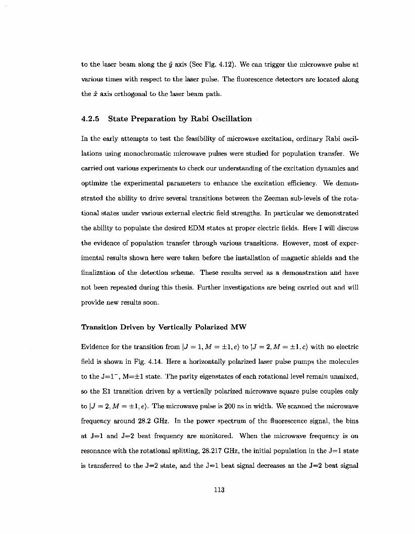
to the laser beam along the y axis (See Fig. 4.12). We can trigger the microwave pulse at
various times with respect to the laser pulse. The fluorescence detectors are located along
the x axis orthogonal to the laser beam path.
4.2.5 State Preparation by Rabi Oscillation
In the early attempts to test the feasibility of microwave excitation, ordinary Rabi oscil
lations using monochromatic microwave pulses were studied for population transfer. We
carried out various experiments to check our understanding of the excitation dynamics and
optimize the experimental parameters to enhance the excitation efficiency. We demon
strated the ability to drive several transitions between the Zeeman sub-levels of the rota
tional states under various external electric field strengths. In particular we demonstrated
the ability to populate the desired EDM states at proper electric fields. Here I will discuss
the evidence of population transfer through various transitions. However, most of exper
imental results shown here were taken before the installation of magnetic shields and the
finalization of the detection scheme. These results served as a demonstration and have
not been repeated during this thesis. Further investigations are being carried out and will
provide new results soon.
Transition Driven by Vertically Polarized MW
Evidence for the transition from \J = 1,M = ±1, e) to |J = 2, M = ±1 , e) with no electric
field is shown in Fig. 4.14. Here a horizontally polarized laser pulse pumps the molecules
to the J= l~ , M=±l state. The parity eigenstates of each rotational level remain unmixed,
so the El transition driven by a vertically polarized microwave square pulse couples only
t o | J = 2,M = ±l ,e) . The microwave pulse is 200 ns in width. We scanned the microwave
frequency around 28.2 GHz. In the power spectrum of the fluorescence signal, the bins
at J = l and J=2 beat frequency are monitored. When the microwave frequency is on
resonance with the rotational splitting, 28.217 GHz, the initial population in the J = l state
is transferred to the J=2 state, and the J = l beat signal decreases as the J=2 beat signal
113
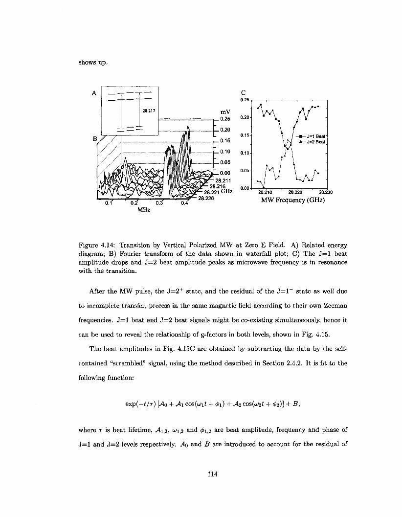
shows up.
28.210 28.220 28.230
MW Frequency (GHz)
Figure 4.14: Transition by Vertical Polarized MW at Zero E Field. A) Related energy diagram; B) Fourier transform of the data shown in waterfall plot; C) The J = l beat amplitude drops and J=2 beat amplitude peaks as microwave frequency is in resonance with the transition.
After the MW pulse, the J = 2 + state, and the residual of the J = l ~ state as well due
to incomplete transfer, precess in the same magnetic field according to their own Zeeman
frequencies. J = l beat and J=2 beat signals might be co-existing simultaneously, hence it
can be used to reveal the relationship of g-factors in both levels, shown in Fig. 4.15.
The beat amplitudes in Fig. 4.15C are obtained by subtracting the data by the self-
contained "scrambled" signal, using the method described in Section 2.4.2. It is fit to the
following function:
exp(- i / r ) [Ao + A\ cos{u)\t + 4>\) + A?cos(u>2i + ^2)] + B,
where r is beat lifetime, .41,2, <^\,2 and ^1,2 are beat amplitude, frequency and phase of
J = l and J=2 levels respectively. AQ and B are introduced to account for the residual of
114
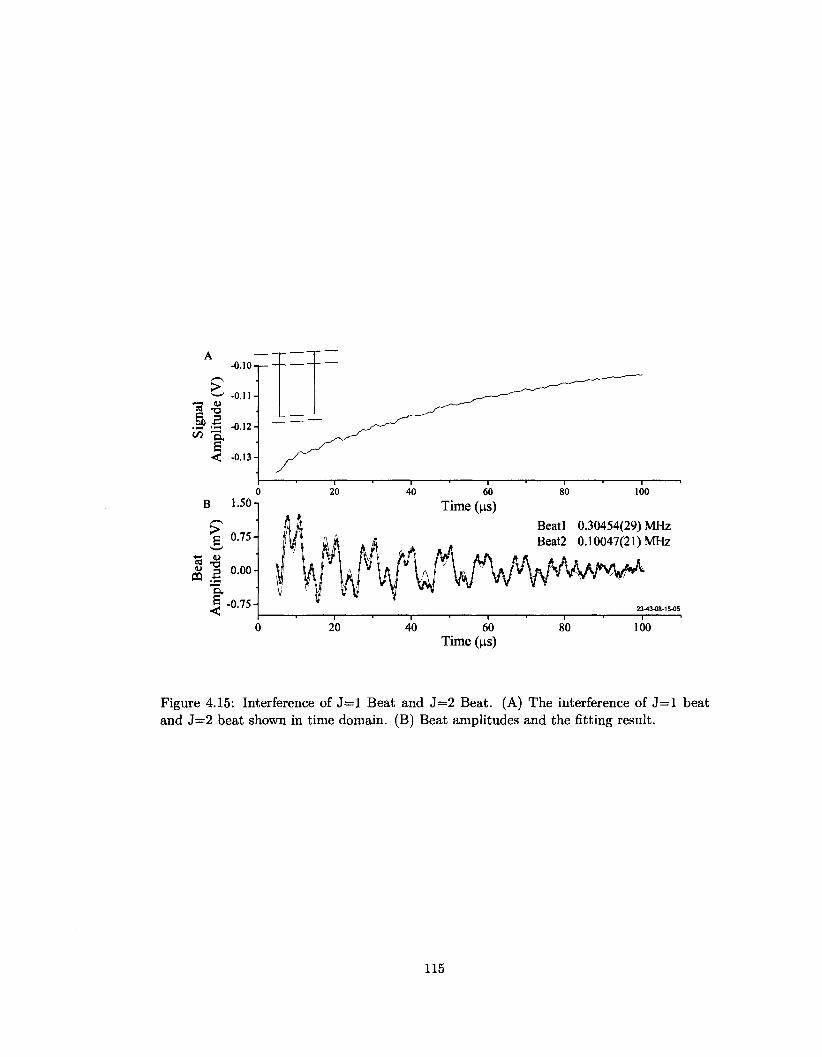
0 B 1.50
>
•B » TO «r-J
m 2
0.75 4
0.00
_§ -0.75-
0 20
40 60 Time (JJ.S)
80
Beatl 0.30454(29) MHz Beat2 0.10047(21) MHz
23-43-08-15-05
40 60 Time (us)
80 100
Figure 4.15: Interference of J = l Beat and 3=2 Beat. (A) The interference of J = l beat and J = 2 beat shown in time domain. (B) Beat amplitudes and the fitting result.
115
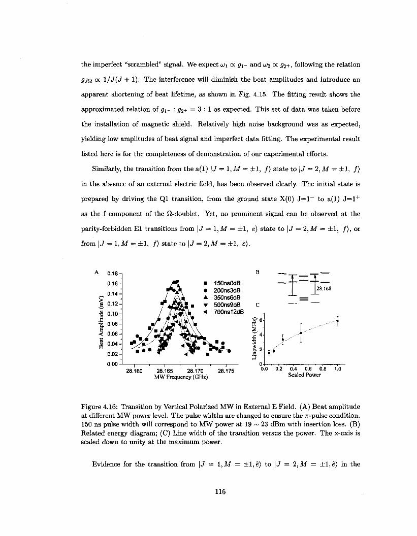
the imperfect "scrambled" signal. We expect UJ\ oc g±- and U2 oc g2+, following the relation
9Jii oc l/J{J + 1). The interference will diminish the beat amplitudes and introduce an
apparent shortening of beat lifetime, as shown in Fig. 4.15. The fitting result shows the
approximated relation of g±- : p2+ = 3 : 1 as expected. This set of data was taken before
the installation of magnetic shield. Relatively high noise background was as expected,
yielding low amplitudes of beat signal and imperfect data fitting. The experimental result
listed here is for the completeness of demonstration of our experimental efforts.
Similarly, the transition from the a(l) | J = 1, M = ±1, / ) state to | J = 2, M = ±1 , / )
in the absence of an external electric field, has been observed clearly. The initial state is
prepared by driving the Ql transition, from the ground state X(0) J = l ~ to a(l) J = l +
as the f component of the fi-doublet. Yet, no prominent signal can be observed at the
parity-forbidden El transitions from |J = 1, M = ±1, e) state to \J — 2,M = ±1 , / ) , or
from \J = 1,M = ±1, / ) state to \J = 2,M = ±1, e).
A
|
Am
plitu
de
Bea
t
0.181
0.16-
0.14-
0.12-
0.10-
0.08-
0.06-
0.04-
0.02-
0.00 J
• 150ns0dB • 200ns3dB A 350ns6dB • 500ns9dB < 700ns12dB
— i • 1 • 1 • 1 28.160 28.165 28.170 28.175
MW Frequency (GHz)
W 6 X
a 2 B
28.168
y \
0.0 0.2 0.4 0.6 0.8 1.0 Scaled Power
Figure 4.16: Transition by Vertical Polarized MW in External E Field. (A) Beat amplitude at different MW power level. The pulse widths are changed to ensure the 7r-pulse condition. 150 ns pulse width will correspond to MW power at 19 ~ 23 dBm with insertion loss. (B) Related energy diagram; (C) Line width of the transition versus the power. The x-axis is scaled down to unity at the maximum power.
Evidence for the transition from \J = 1,M — ±l ,e) to \J = 2,M = ± l ,e ) in the
116
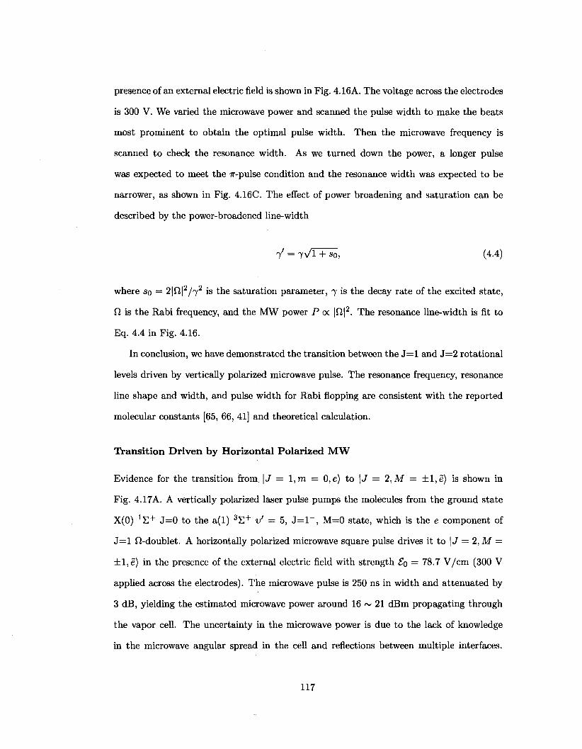
presence of an external electric field is shown in Fig. 4.16A. The voltage across the electrodes
is 300 V. We varied the microwave power and scanned the pulse width to make the beats
most prominent to obtain the optimal pulse width. Then the microwave frequency is
scanned to check the resonance width. As we turned down the power, a longer pulse
was expected to meet the 7r-pulse condition and the resonance width was expected to be
narrower, as shown in Fig. 4.16C. The effect of power broadening and saturation can be
described by the power-broadened line-width
V = 7VI + so, (4.4)
where so = 2j!Ti|2/-y2 is the saturation parameter, 7 is the decay rate of the excited state,
fi is the Rabi frequency, and the MW power P oc |fi|2. The resonance line-width is fit to
Eq. 4.4 in Fig. 4.16.
In conclusion, we have demonstrated the transition between the J = l and J=2 rotational
levels driven by vertically polarized microwave pulse. The resonance frequency, resonance
line shape and width, and pulse width for Rabi flopping are consistent with the reported
molecular constants [65, 66, 41] and theoretical calculation.
Transition Driven by Horizontal Polarized MW
Evidence for the transition from. \J = l ,m = 0,e) to \J = 2,M = ± l ,e) is shown in
Fig. 4.17A. A vertically polarized laser pulse pumps the molecules from the ground state
X(0) 1 E + J=0 to the a(l) 3 S + v' = 5, J= l~ , M=0 state, which is the e component of
J = l fi-doublet. A horizontally polarized microwave square pulse drives it to \J — 2, M =
±l ,e) in the presence of the external electric field with strength £0 = 78.7 V/cm (300 V
applied across the electrodes). The microwave pulse is 250 ns in width and attenuated by
3 dB, yielding the estimated microwave power around 16 ~ 21 dBm propagating through
the vapor cell. The uncertainty in the microwave power is due to the lack of knowledge
in the microwave angular spread in the cell and reflections between multiple interfaces.
117
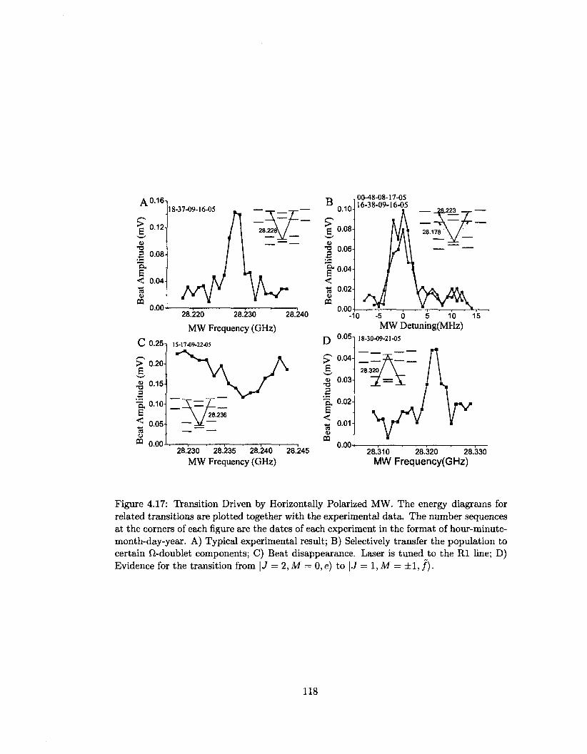
A0.16,
I 0.12-
t3 5 0.08 "E, S < 0.04 13
0.00
18-37-09-16-05
, 00-48-08-17-05 16-38-09-16-05
C 0.25
> 0.20
Jg 0.15
^ 0.05
m 0.00
28.220 28.230 28.240
MW Frequency (GHz)
15-17-09-22-05
\ / 28.236
28.230 28.235 28.240 28.245 MW Frequency (GHz)
D
-5 0 5 10 15 MW Detuning(MHz)
° - 0 5 T 18-30-09-21-05
> 0.04
Hi 0-03-a •g, 0.02 s « 0.01
pa 0.00 28.310 28.320 28.330
MW Frequency(GHz)
Figure 4.17: Transition Driven by Horizontally Polarized MW. The energy diagrams for related transitions are plotted together with the experimental data. The number sequences at the corners of each figure are the dates of each experiment in the format of hour-minute-month-day-year. A) Typical experimental result; B) Selectively transfer the population to certain Q-doublet components; C) Beat disappearance. Laser is tuned to the Rl line; D) Evidence for the transition from | J = 2,M = 0,e) to |J = 1, M = ±1, / ) .
118
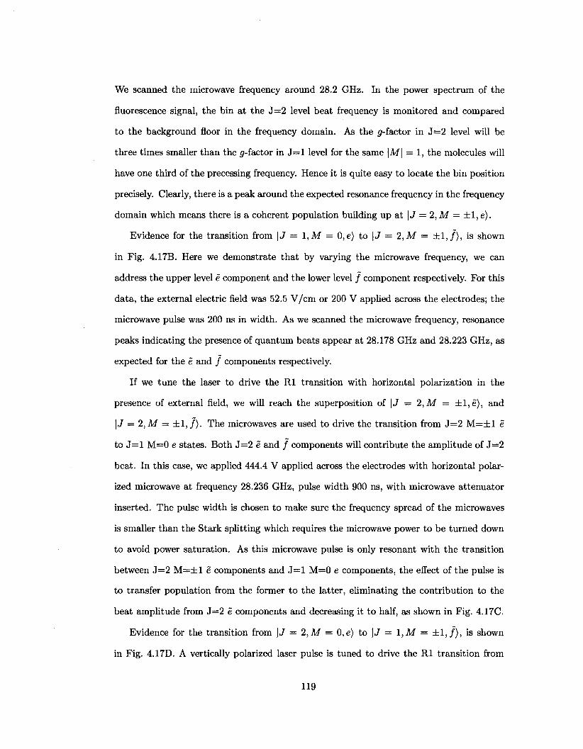
We scanned the microwave frequency around 28.2 GHz. In the power spectrum of the
fluorescence signal, the bin at the J=2 level beat frequency is monitored and compared
to the background floor in the frequency domain. As the g-factor in J=2 level will be
three times smaller than the p-factor in J = l level for the same \M\ = 1, the molecules will
have one third of the precessing frequency. Hence it is quite easy to locate the bin position
precisely. Clearly, there is a peak around the expected resonance frequency in the frequency
domain which means there is a coherent population building up at | J = 2, M = ±1, e).
Evidence for the transition from \J = 1,M = 0,e) to \J = 2,M = ±1 , / ) , is shown
in Fig. 4.17B. Here we demonstrate that by varying the microwave frequency, we can
address the upper level e component and the lower level / component respectively. For this
data, the external electric field was 52.5 V/cm or 200 V applied across the electrodes; the
microwave pulse was 200 ns in width. As we scanned the microwave frequency, resonance
peaks indicating the presence of quantum beats appear at 28.178 GHz and 28.223 GHz, as
expected for the e and / components respectively.
If we tune the laser to drive the Rl transition with horizontal polarization in the
presence of external field, we will reach the superposition of \J = 2,M = ± l ,e ) , and
\J = 2,M = ±1 , / ) . The microwaves are used to drive the transition from J=2 M = ± l e
to J = l M=0 e states. Both J=2 e and / components will contribute the amplitude of 3—2
beat. In this case, we applied 444.4 V applied across the electrodes with horizontal polar
ized microwave at frequency 28.236 GHz, pulse width 900 ns, with microwave attenuator
inserted. The pulse width is chosen to make sure the frequency spread of the microwaves
is smaller than the Stark splitting which requires the microwave power to be turned down
to avoid power saturation. As this microwave pulse is only resonant with the transition
between J=2 M=±l e components and J = l M=0 e components, the effect of the pulse is
to transfer population from the former to the latter, eliminating the contribution to the
beat amplitude from 3=2 e components and decreasing it to half, as shown in Fig. 4.17C.
Evidence for the transition from \J = 2,M = 0, e) to \J = 1,M = ± 1 , / ) , is shown
in Fig. 4.17D. A vertically polarized laser pulse is tuned to drive the Rl transition from
119
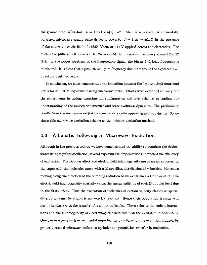
the ground state X(0) J= l~ v = 1 to the a(l) J=2 + , M=0 v' = 5 state. A horizontally
polarized microwave square pulse drives it down to \J = 1,M = ±l ,e) in the presence
of the external electric field of 116.54 V/cm or 444 V applied across the electrodes. The
microwave pulse is 350 ns in width. We scanned the microwave frequency around 28.322
GHz. In the power spectrum of the fluorescence signal, the bin at J = l beat frequency is
monitored. It is clear that a peak shows up in frequency domain right at the expected J = l
quantum beat frequency.
In conclusion, we have demonstrated the transition between the J = l and J=2 rotational
levels for the EDM experiment using microwave pulse. Efforts were extended to carry out
the experiments in various experimental configuration and level schemes to confirm our
understanding of the molecular structure and state evolution dynamics. The preliminary
results from the microwave excitation scheme were quite appealing and convincing. So we
chose this microwave excitation scheme as the primary excitation method.
4.3 Adiabatic Following in Microwave Excitation
Although in the previous section we have demonstrated the ability to populate the desired
states using 7r-pulses oscillation, several experimental imperfections hampered the efficiency
of excitation. The Doppler effect and electric field inhomogeneity are of major concern. In
the vapor cell, the molecules move with a Maxwellian distribution of velocities. Molecules
moving along the direction of the pumping radiation beam experience a Doppler shift. The
electric field inhomogeneity spatially varies the energy splitting of each fi-doublet level due
to the Stark effect. Thus the excitation of molecules of certain velocity classes or spatial
distributions and locations, is not exactly resonant. Hence their population transfer will
not be in phase with the transfer of resonant molecules. These velocity-dependent interac
tions and the inhomogeneity of electromagnetic field diminish the excitation probabilities.
One can overcome such experimental imperfection by adiabatic time evolution induced by
properly crafted microwave pulses to optimize the population transfer in molecules.
120
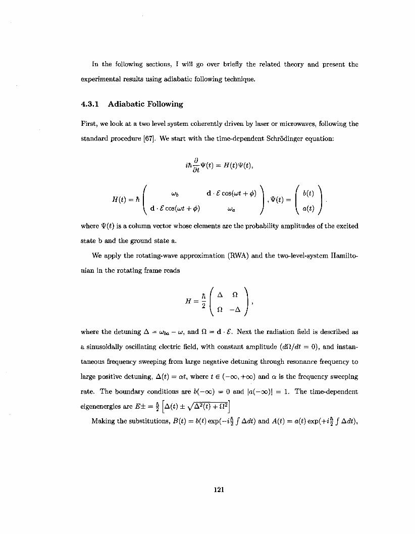
In the following sections, I will go over briefly the related theory and present the
experimental results using adiabatic following technique.
4.3.1 Adiabatic Following
First, we look at a two level system coherently driven by laser or microwaves, following the
standard procedure [67]. We start with the time-dependent Schrodinger equation:
iftJU(i) = H{t)9(t),
(
H{t) = h \
, * ( * ) = ' m ^ J \ o(*) /
UJI, d • £ cos(wt + <j>)
\ d • £ cos(utf + 4>) uja
where \I/(£) is a column vector whose elements are the probability amplitudes of the excited
state b and the ground state a.
We apply the rotating-wave approximation (RWA) and the two-level-system Hamilto-
nian in the rotating frame reads
-I /
V A n fl - A
where the detuning A = u>ba — u), and Q = d • £. Next the radiation field is described as
a sinusoidally oscillating electric field, with constant amplitude (dfl/dt = 0), and instan
taneous frequency sweeping from large negative detuning through resonance frequency to
large positive detuning, A(t) = at, where t € (—oo, -l-oo) and a is the frequency sweeping
rate. The boundary conditions are b(—oo) = 0 and |o(—oc)| = 1. The time-dependent
eigenenergies are E± = | A(t) ± ^/A2(t) + Q,2
Making the substitutions, B{t) = b(t) e x p ( - i | / Adt) and A(t) = a(t) exp(+i | / Adt),
121
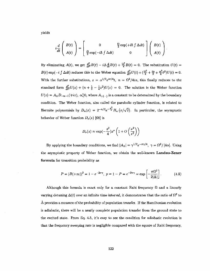
yields
0 % exp(+ih f Adt)
§ exp(-»ft / A * ) 0
By eliminating A(t), we get J^-B(t) - iAftB{t) + f B ( t ) = 0. The substitution U(t) =
B(t) exp(-t / Adt) reduces this to the Weber equation ^U(t) + {i-j- + f + ^t2)U{t) = 0.
With the further substitutions, z = all2e%,KlH, n = $l2/4ia, this finally reduces to the
standard form M?U(Z) + (n + \ — \z2)U(z) = 0. The solution is the Weber function
U(z) = A±D-n-i(^iz), a<0, where -A+(-) is a constant to be determined by the boundary
condition. The Weber function, also called the parabolic cylinder function, is related to 2
Hermite polynomials by Dn(x) = 2~nl2e~~* Hn (x/\/2). In particular, the asymptotic
behavior of Weber function Dl/(z) [68] is
Dv{z)*ew{-j)zv(l + oK
By applying the boundary conditions, we find \A±\ = 71/2e~,r7/'4, 7 = ft2/ |4a|. Using
the asymptotic property of Weber function, we obtain the well-known Landau-Zener
formula for transition probability as
P = |£(+oo)|2 = 1 - e " 2 ^ , p = 1 - P = e~2^ = exp TTfi2
2|A| (4.5)
Although this formula is exact only for a constant Rabi frequency Q. and a linearly
varying detuning A(t) over an infinite time interval, it demonstrates that the ratio of O2 to
A provides a measure of the probability of population transfer. If the Hamiltonian evolution
is adiabatic, there will be a nearly complete population transfer from the ground state to
the excited state. Prom Eq. 4.5, it's easy to see the condition for adiabatic evolution is
that the frequency sweeping rate is negligible compared with the square of Rabi frequency,
122
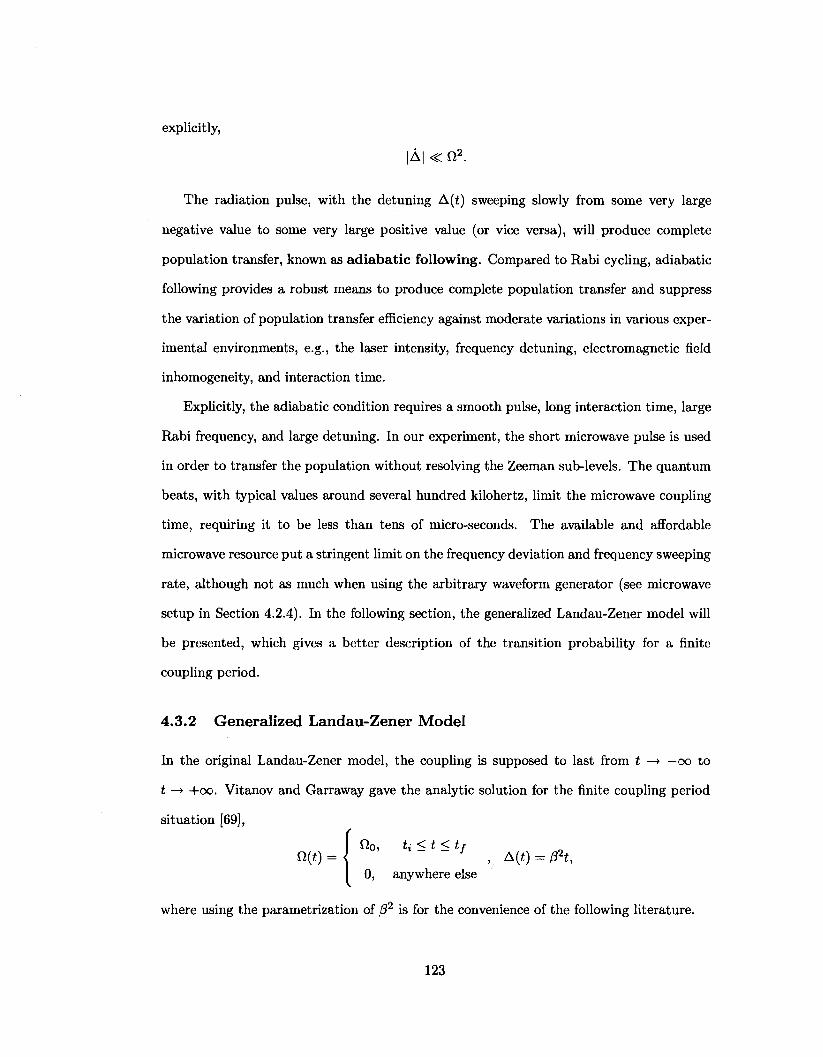
explicitly,
|A| < n2.
The radiation pulse, with the detuning A(t) sweeping slowly from some very large
negative value to some very large positive value (or vice versa), will produce complete
population transfer, known as adiabatic following. Compared to Rabi cycling, adiabatic
following provides a robust means to produce complete population transfer and suppress
the variation of population transfer efficiency against moderate variations in various exper
imental environments, e.g., the laser intensity, frequency detuning, electromagnetic field
inhomogeneity, and interaction time.
Explicitly, the adiabatic condition requires a smooth pulse, long interaction time, large
Rabi frequency, and large detuning. In our experiment, the short microwave pulse is used
in order to transfer the population without resolving the Zeeman sub-levels. The quantum
beats, with typical values around several hundred kilohertz, limit the microwave coupling
time, requiring it to be less than tens of micro-seconds. The available and affordable
microwave resource put a stringent limit on the frequency deviation and frequency sweeping
rate, although not as much when using the arbitrary waveform generator (see microwave
setup in Section 4.2.4). In the following section, the generalized Landau-Zener model will
be presented, which gives a better description of the transition probability for a finite
coupling period.
4.3.2 Generalized Landau-Zener Model
In the original Landau-Zener model, the coupling is supposed to last from t —• -co to
t —> +00. Vitanov and Garraway gave the analytic solution for the finite coupling period
situation [69],
^Oi ti < t < tf
«(*) = < - m = p%
0, anywhere else
where using the parametrization of /?2 is for the convenience of the following literature.
123
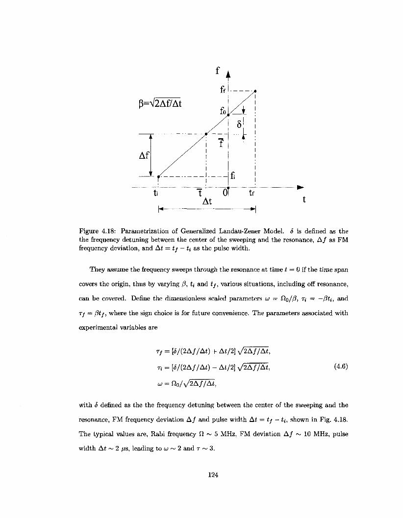
P=V2Af/At
Figure 4.18: Parametrization of Generalized Landau-Zener Model. 6 is defined as the the frequency detuning between the center of the sweeping and the resonance, A / as FM frequency deviation, and At = tf — ti as the pulse width.
They assume the frequency sweeps through the resonance at time t = 0 if the time span
covers the origin, thus by varying /?, ti and tf, various situations, including off resonance,
can be covered. Define the dimensionless scaled parameters u> = Ho//?, Tj = — /?ij, and
Tf = @tf, where the sign choice is for future convenience. The parameters associated with
experimental variables are
Tf = [5/(2Af/At) + At/2] y/2Af/At,
n = [6/(2Af/At) - At/2] y/2Af/At,
UJ = n 0 / \ / 2 A / / A i ,
(4.6)
with 8 defined as the the frequency detuning between the center of the sweeping and the
resonance, FM frequency deviation A / and pulse width At = tf - U, shown in Fig. 4.18.
The typical values are, Rabi frequency Q. ~ 5 MHz, FM deviation A / ~ 10 MHz, pulse
width At ~ 2 /xs, leading to u> ~ 2 and r ~ 3.
124
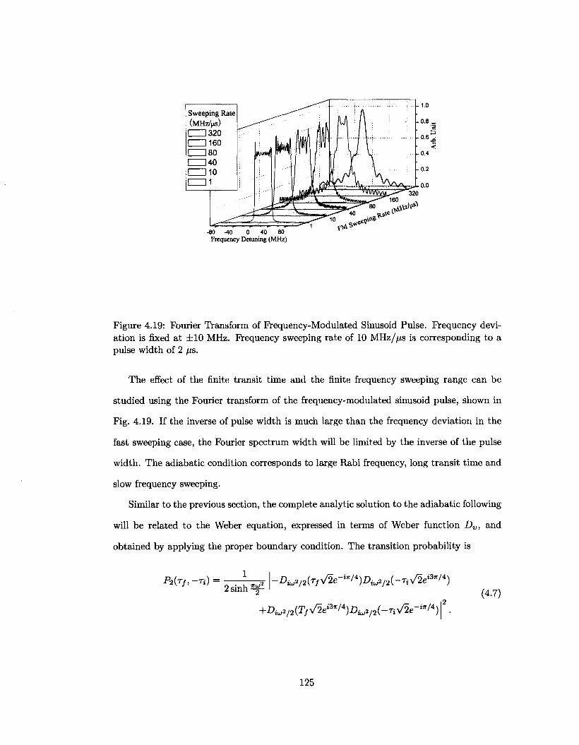
160 . 80 ^
-80 -40 0 40 80 Frequency Detuning (MHz)
^ * e
Figure 4.19: Fourier Transform of Frequency-Modulated Sinusoid Pulse. Frequency deviation is fixed at ±10 MHz. Frequency sweeping rate of 10 MHz/fis is corresponding to a pulse width of 2 fis.
The effect of the finite transit time and the finite frequency sweeping range can be
studied using the Fourier transform of the frequency-modulated sinusoid pulse, shown in
Fig. 4.19. If the inverse of pulse width is much large than the frequency deviation in the
fast sweeping case, the Fourier spectrum width will be limited by the inverse of the pulse
width. The adiabatic condition corresponds to large Rabi frequency, long transit time and
slow frequency sweeping.
Similar to the previous section, the complete analytic solution to the adiabatic following
will be related to the Weber equation, expressed in terms of Weber function Dv, and
obtained by applying the proper boundary condition. The transition probability is
Fi(Tf, -Ti) = 1
2 sinh 2^1 -Dilt?/2(Tfy/2e-i*'*)Dij2/2{-ny/2eia'/4)
+DiiJy2(TfV2ei^4)Di(Jy2(-nV2e-i^4)
(4.7)
125
The adiabatic solution is obtained in the condition u » 1 is
p . ^ 1 , ZlH ^ « M K ( T / ) + ^ ( T < ) 1 -T2(T/, - T j J ~ - H , , ,
where
£(T) = T \ / T 2 + UJ2 + UJ2 In r + v r 2 + u2
w
The asymptotic expression under the strong-coupling condition r 2 + UJ2 » 1 and
TJ + LJ2 » 1 is
1 / l ft(r/, -Ti) ~ - + I - - e
TiTj
7TU>
e 2
v/(a>2 + r2)(u;2 + T2)
^J^ + TJ^ + T2)
COS_£(T/) cosg(Tj) r /
a; + •
{ e - ^ 2 cos [g(T/) - gfo)] - (1 - e ~ ^ 2 ) cos R( T / ) + £ ( T Q ] }
2y/{u;2 + T2)(uJ2 + r?)
It is readily verified that the strong-coupling asymptotic approximation contains the adi
abatic following approximation in the limit u> » 1, and it can be used to describe the
weak-coupling asymptotic situation in the limit Tj, Tf » UJ.
For symmetric crossing, with Tj = Tf, the transition probability is
P-Z(T, - T ) ~ 1 - e"
,2
TTCtl2 /
— e 2 V I — e~ ™Srz^cos£>) or + T
+ U)
UJ2 + T2 e~™ - (1 - e"™ ) cos2 £ > )
where
f ( r ) = - - ^ - + TV /r2 + w2 + w2 ln 4 2
- T = ( T + VT2 + UJ2) v 2
+ a r g r ( l - - i w 2 ) .
Evidently, Eq. 4.3.2 reduces to the well known Landau-Zener formula for infinite coupling
126
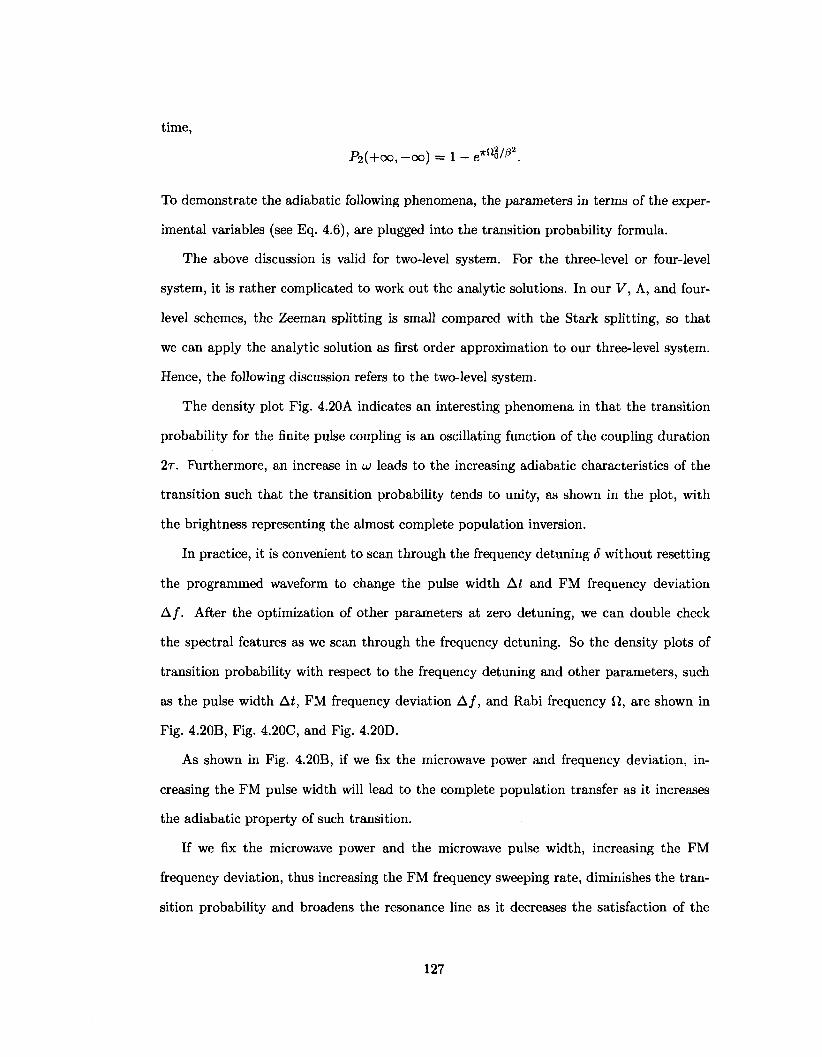
time,
P2(+cx),-oo) = l-e' r J lo//32.
To demonstrate the adiabatic following phenomena, the parameters in terms of the exper
imental variables (see Eq. 4.6), are plugged into the transition probability formula.
The above discussion is valid for two-level system. For the three-level or four-level
system, it is rather complicated to work out the analytic solutions. In our V, A, and four-
level schemes, the Zeeman splitting is small compared with the Stark splitting, so that
we can apply the analytic solution as first order approximation to our three-level system.
Hence, the following discussion refers to the two-level system.
The density plot Fig. 4.20A indicates an interesting phenomena in that the transition
probability for the finite pulse coupling is an oscillating function of the coupling duration
2r. Furthermore, an increase in u) leads to the increasing adiabatic characteristics of the
transition such that the transition probability tends to unity, as shown in the plot, with
the brightness representing the almost complete population inversion.
In practice, it is convenient to scan through the frequency detuning S without resetting
the programmed waveform to change the pulse width At and FM frequency deviation
A/ . After the optimization of other parameters at zero detuning, we can double check
the spectral features as we scan through the frequency detuning. So the density plots of
transition probability with respect to the frequency detuning and other parameters, such
as the pulse width At, FM frequency deviation A/ , and Rabi frequency fi, are shown in
Fig. 4.20B, Fig. 4.20C, and Fig. 4.20D.
As shown in Fig. 4.20B, if we fix the microwave power and frequency deviation, in
creasing the FM pulse width will lead to the complete population transfer as it increases
the adiabatic property of such transition.
If we fix the microwave power and the microwave pulse width, increasing the FM
frequency deviation, thus increasing the FM frequency sweeping rate, diminishes the tran
sition probability and broadens the resonance line as it decreases the satisfaction of the
127
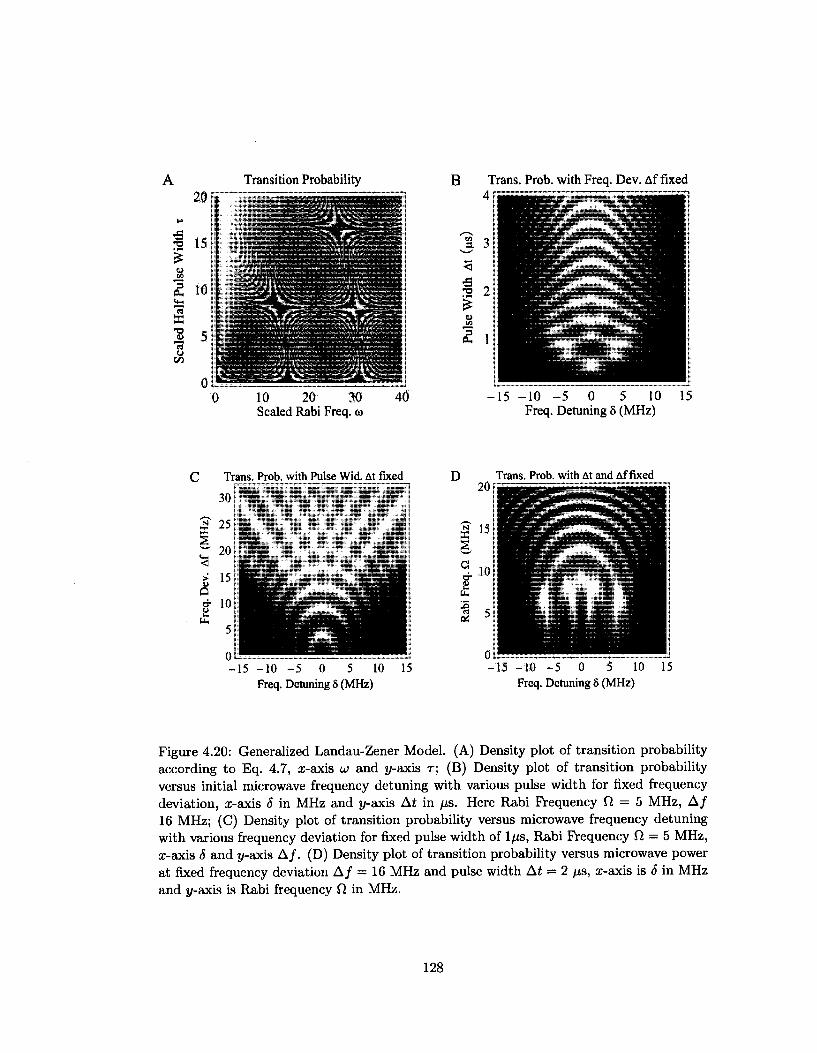
A Transition Probability B Trans. Prob. with Freq. Dev. Affixed
C Trans. Prob. with Pulse Wid. At fixed D Trans. Prob. with At and Affixed
Freq. Detuning 8 (MHz) Freq. Detuning 8 (MHz)
Figure 4.20: Generalized Landau-Zener Model. (A) Density plot of transition probability according to Eq. 4.7, ac-axis u and y-axis r; (B) Density plot of transition probability versus initial microwave frequency detuning with various pulse width for fixed frequency deviation, rc-axis S in MHz and y-axis Ai in fj,s. Here Rabi Frequency fi = 5 MHz, A / 16 MHz; (C) Density plot of transition probability versus microwave frequency detuning with various frequency deviation for fixed pulse width of 1/xs, Rabi Frequency CI = 5 MHz, x-axis 8 and y-axis A/ . (D) Density plot of transition probability versus microwave power at fixed frequency deviation A / = 16 MHz and pulse width At = 2 /xs, rc-axis is S in MHz and y-axis is Rabi frequency Q in MHz.
128
Af CZD 32MHz CZ316MHz CZH8MHZ CZZHMHz CZD2MHZ
32MHz
* -20 0 20 Detuning 8 (MHz)
^>"2MHz %mz ^ V *
(A)
-40 -20 0 20 40 Detuning 8 (MHz)
(B)
Figure 4.21: Transition Probability at Different Frequency Deviation and Power using Adiabatic Following, calculated using Eq. 4.7. (A) Transition probability at different frequency deviations A/ . Here Rabi Frequency fi is fixed at 4.5 MHz, and pulse width At = tf — ti = 2 fj,s. (B) Transition probability at different Rabi frequencies. Here frequency deviation A / is fixed at 11 MHz, and pulse width At = 2 /is.
129
adiabatic condition, shown in Fig. 4.20C. Insufficient FM frequency deviation results in
a short coupling time r (see Eq. 4.6), leading to incomplete population transfer, shown
in Fig. 4.21A. If we fix the frequency sweeping rate and span, increasing the microwave
power moves the condition of transition into the adiabatic regime with increasing transition
probability, shown in Fig. 4.20D. Increasing microwave power broadens the resonance line
width, as shown in Fig. 4.21B.
As emphasized previously, the above discussion is valid for two-level system. The
application to our three-level or four-level system is just an approximation. But still, the
analytic solution serves as a general guidance for the choice of the parameter range of
the pulse width, sweeping frequency, and Rabi frequency. The experiments to check the
validity of the analytic solution and the modification to our specific level schemes were
carried out and will be discussed in the next section.
4.3.3 Adiabatic Following Experiment
The experimental results using the adiabatic following technique are presented here. A
carefully engineered control voltage is applied to the external control port of the Agilent
E8257C for frequency modulation. To avoid spurious effects, we turn on the frequecy
modulation a few yxs before the pulse and hold it at the low(high) voltage, ramp the
voltage from low to high (or vice versa) during the pulse span, and turn it off at few ps
after turning off the microwave switch.
The typical experimental result using the adiabatic following technique is shown in
Fig. 4.22.
A vertically polarized laser pulse tuned to the RO line pumps the molecules from the
ground state to the a(l) 3 S + J= l~ , M=0 state. A horizontally polarized microwave square
pulse then drives them to \J = 2, M — ± l ,e) in the presence of the external electric field
with strength 78.7 V/cm. The microwave pulse is 2 /xs in width and attenuated by 3 dB,
with the frequency modulation mode on at 7.5 MHz deviation. The microwave power is
estimated to be around 24 dBm inside the cell, corresponding to a Rabi frequency QQ ^
130
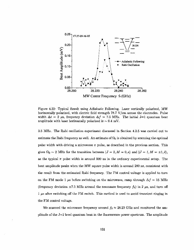
0.25-1
0.20
o 0.15
a "I* 0.10 <
& 0.05
0.00
" 17-37-09-16-05
1 "1 \
1 * \
1 * \ / T* A
- • • — i " ' —
Zi=Z_ \ / 28.228
— \1 —
—•— Adiabatic Following v Rabi Oscillation
28.200 28.220 28.240 28.260
MW Center Frequency fo (GHz)
Figure 4.22: Typical Result using Adiabatic Following. Laser vertically polarized, MW horizontally polarized, with electric field strength 78.7 V/cm across the electrodes. Pulse width At = 2 (is, frequency deviation A / = 7.5 MHz. The initial J = l quantum beat amplitude with laser horizontally polarized is ~ 0.4 mV.
3.5 MHz. The Rabi oscillation experiment discussed in Section 4.2.5 was carried out to
estimate the Rabi frequency as well. An estimate of Oo is obtained by scanning the optimal
pulse width with driving a microwave 7r pulse, as described in the previous section. This
gives f)o ~ 2 MHz for the transition between \J = 2,M — 0,e) and \J = 1,M = ± l ,e ) ,
as the typical 7r pulse width is around 500 ns in the ordinary experimental setup. The
beat amplitude peaks when the MW square pulse width is around 280 ns, consistent with
the result from the estimated Rabi frequency. The FM control voltage is applied to turn
on the FM mode 1 fj,s before switching on the microwave, ramp through A / = 15 MHz
(frequency deviation ±7.5 MHz around the resonance frequency /o) in 2 fis, and turn off
1 /J,S after switching off the FM switch. This method is used to avoid transient ringing in
the FM control voltage.
We scanned the microwave frequency around /o « 28.23 GHz and monitored the am
plitude of the J=2 level quantum beat in the fluorescence power spectrum. The amplitude
131

peak indicates coherent population builds up in \J = 2,m = ± l ,e) as the FM center
frequency /o is scanned through the transition resonance. The initial J = l quantum beat
amplitude with laser horizontally polarized is ~ 0.4 mV. The maximum J=2 quantum beat
amplitude using the adiabatic following method is ~ 0.23 mV, shown as the square-solid
line in Fig. 4.22. The spectral shape matches the theoretical calculation of transition prob
ability using Eq. 4.7 with parameter A/=7.5 MHz, At = 2 /xs, and Rabi frequency fio is
3.5 MHz. There is only ~ 0.13 mV J=2 beat amplitude achieved using the Rabi oscillation
method (see Section 4.2.5), shown as the triangle-dotted line in Fig. 4.22. The experi
mental result reflects ~ 70% improvement in the transfer efficiency by using the adiabatic
following.
To ensure the satisfaction of the adiabatic condition u = QQ/\/\A\ <C 1, the Rabi
cycling method described in previous section is carried out first to obtain an estimate of
the Rabi frequency fio- Second, various FM deviations and pulse widths are scanned.
In Fig. 4.23A, the quantum beat amplitude is plotted against the pulse width At with
FM deviation A / fixed at 2 MHz, 5 MHz, 10 MHz, 20 MHz, and 32 MHz respectively,
hence various sweeping rate. Fig. 4.23B shows the quantum beat amplitude versus the FM
deviation A / as the pulse width is fixed at 0.75 /xs, 1 /xs, 2 /xs, and 4 /xs respectively.
For the transition between \J = 1,M = 0,e) and \J = 2,M = ± l , e ) , the optimal
sweeping rate seems to be around 2 ~ 5 MHz//xs, which is consistent with fio ~ 5 MHz,
|A| <?C QQ. It suggests that the frequency sweeping rate should be less than 1.5 MHz//xs.
This requirement is quite consistent with the experimental result. A new amplifier with
higher power output will allow larger Rabi frequency and larger frequency deviation. Fur
ther experiments will be carried out using the microwave amplifier with higher power
output.
We have also explored the parameter space for the optimization of the population trans
fer. If we plot the transition probability against the FM center frequency, the theoretical
prediction of the spectral lines will look like Fig. 4.24A.
However the experimental results, shown in Fig. 4.24B for the transition between \J =
132
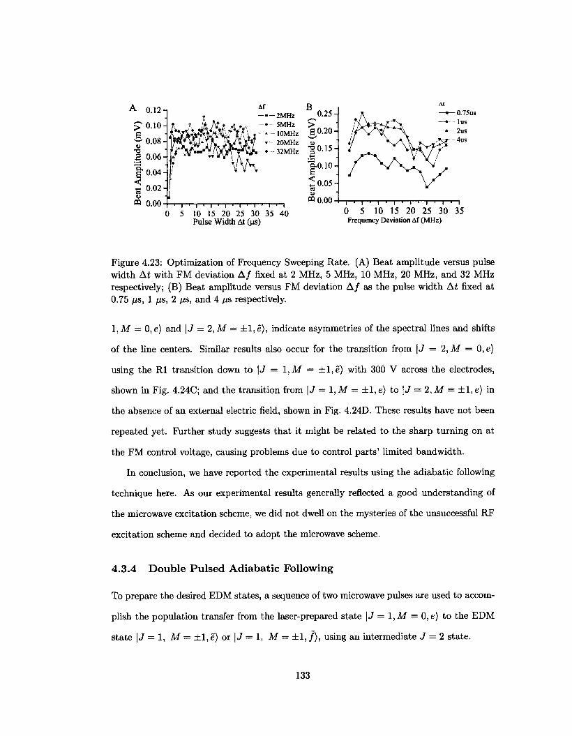
A 0.12
S 0.04-| < ~ 0.02 H ffl o.oo I ' I ' I ' I ' I ' I ' I
0 5 10 15 20 25 30 35 40 Pulse Width At (us)
I ' I ' I " I ' I • I • i 0 5 10 15 20 25 30 35 Frequency Deviation Af (MHz)
Figure 4.23: Optimization of Frequency Sweeping Rate. (A) Beat amplitude versus pulse width At with FM deviation A / fixed at 2 MHz, 5 MHz, 10 MHz, 20 MHz, and 32 MHz respectively; (B) Beat amplitude versus FM deviation A / as the pulse width At fixed at 0.75 fis, 1 /is, 2 yis, and 4 fxs respectively.
1,M — 0, e) and \J = 2,M = ± l ,e ) , indicate asymmetries of the spectral lines and shifts
of the line centers. Similar results also occur for the transition from \J = 2,M = 0,e)
using the Rl transition down to \J = 1,M = ±l ,e) with 300 V across the electrodes,
shown in Fig. 4.24C; and the transition from | J = 1, M = ±1, e) to | J — 2, M = ±1 , e) in
the absence of an external electric field, shown in Fig. 4.24D. These results have not been
repeated yet. Further study suggests that it might be related to the sharp turning on at
the FM control voltage, causing problems due to control parts' limited bandwidth.
In conclusion, we have reported the experimental results using the adiabatic following
technique here. As our experimental results generally reflected a good understanding of
the microwave excitation scheme, we did not dwell on the mysteries of the unsuccessful RF
excitation scheme and decided to adopt the microwave scheme.
4.3.4 Double Pulsed Adiabatic Following
To prepare the desired EDM states, a sequence of two microwave pulses are used to accom
plish the population transfer from the laser-prepared state \J = \,M = 0, e) to the EDM
state |J = 1, M = ±1,e) or | J = 1, M = ±1 , / ) , using an intermediate 3 = 2 state.
133
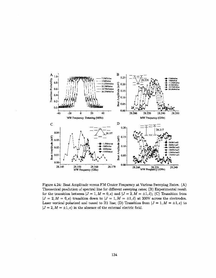
!
7.5MHz2us — 15MHz4us
ll.25MHz3us - - 22.5MHz6us
I8.75MHz6us 26.25MHz7us
-20 0 20 40
MW Frequency Detuning (MHz)
0.04-
0.03-
0.02-
0.01-
0.00-
^ \ M / \
/ \ / , i / ii j-i A 1J l ^AF • •
JYl [
w
_ A / \_28.157 ~~ =
-•-l.SMHzlus - • 3MHz2us A- 6MHz4us
- f 12MHz8us ,*.
A
m- 7.5MHz2us • 15MHZ4U8 A-11.25MHZ3US Y 22.5MHz6us 4 - 18.7SMHZ6US • 26.25MHz7u»
28.200 28.220 28.240
MW Frequency (GHz)
D 0.20n
£-0.15
0.10-
28.140 28.150 28.160 M W Frequency (GHz)
28.170 0.00
28.260
' -B-5MHzlusJ2 -•-SMHzlusJl -A-10MHzlu»J2
^ lOMHzlusJI 15MHzlusJ2
• 15MHzlusJl *
28.200 28.220 MW Frequency (GHz)
28.240
Figure 4.24: Beat Amplitude versus FM Center Frequency at Various Sweeping Rates. (A) Theoretical prediction of spectral line for different sweeping rates; (B) Experimental result for the transition between \J = 1,M = 0,e) and | J = 2,M = ±l ,e ) ; (C) Transition from \J = 2,M = 0,e) transition down to \J = 1,M = ±l ,e) at 300V across the electrodes. Laser vertical polarized and tuned to Rl line; (D) Transition from |J = l , M = ± l , e ) t o |J = 2,M = ±l ,e) in the absence of the external electric field.
134
As described in the previous section, we first prepare the molecules in the | J = 1, M =
0, e) state. Two microwave pulses with different polarizations and frequencies are required
and made possible by a microwave orthomode transducer (OMT) and conical horn. We
apply an adiabatic following technique to both pulses to pursue better population transfer
efficiency. For our current setup with a single microwave source, the separated microwave
pulses first transfer the population to the a(l) J=2 level, then transfer down to the desired
EDM states in separate single-photon steps. For each individual step, we follow experimen
tal procedures similar to those in last section. In addition to the experimental parameter
space we explored, the time delay between two consecutive pulses can be optimized as well.
The scheme using chirped adiabatic passage with overlapping pulse sequence to populate
the desired states selectively [70] is under consideration for future improvements.
The significant achievement in the microwave adiabatic following experiment is to se
lectively populate the EDM states with a good efficiency. Fig. 4.25A shows the population
transfer steps, first applying horizontal microwave to drive from \J = 1,M = 0, e) to
| J = 2,M = ±l ,e ) , then applying vertical microwave to drive down t o | J = l , M = ±l ,e ) .
The laser is vertically polarized and tuned to R0 line, and electric field strength is 39 V/cm.
The first MW pulse has At = 2 /is pulse width, is centered at fQ = 28.220 GHz, and has
a A / = 11 MHz frequency deviation; The second pulse has At = 2 fis pulse width, is
centered at /Q' = 28.193 GHz, and has a A / = 11 MHz frequency deviation, with 0.5 /is
delay after the first pulse. The dashed line shows the J = l beat amplitude when the laser
is horizontally polarized, denoting the available molecules in J = l levels. The dotted line
shows the J=2 beat amplitude after the first microwave pulse and the solid line shows the
J = l beat amplitude after the second microwave pulse, compared with the original J = l
beat amplitude, yielding around 43% efficiency and 3% quantumn beat contrast.
Fig. 4.25B shows another population transfer path, first applying vertical polarized
microwaves to drive from | J = 1, M = 0, e) to | J = 2, M = 0, e), then applying horizontally
polarized microwaves to drive down to \J = 1,M = ±l ,e) . Here first MW pulse has a
At = 2 fis pulse width, is centered at fQ = 28.217 GHz, and has an A / = 11 MHz frequency
135
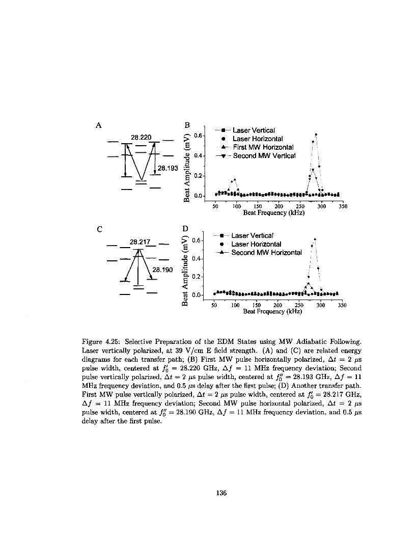
28.220
28.193 5
28.217
B - 0 . 6
J 0.4 a | 0.2 <
3 o.o
D
28.190 £
> £ 13
a s < ts <u «
0.6
0.4
0.2
0.0
Laser Vertical Laser Horizontal First MW Horizontal Second MW Vertical
•*,*»*it|*»»m.*t»m»*f»|!
50 100 150 200 250 Beat Frequency (kHz)
Laser Vertical Laser Horizontal Second MW Horizontal
300 350
> > 'Hthu» a i t int lJt iut>Hni , .»t lu»i
50 100 150 200 250 Beat Frequency (kHz)
300 350
Figure 4.25: Selective Preparation of the EDM States using MW Adiabatic Following. Laser vertically polarized, at 39 V/cm E field strength. (A) and (C) are related energy diagrams for each transfer path; (B) First MW pulse horizontally polarized, At = 2 fis pulse width, centered at /Q = 28.220 GHz, A / = 11 MHz frequency deviation; Second pulse vertically polarized, At = 2 /us pulse width, centered at /Q = 28.193 GHz, A / = 11 MHz frequency deviation, and 0.5 /is delay after the first pulse; (D) Another transfer path. First MW pulse vertically polarized, At = 2 (j,s pulse width, centered at /Q = 28.217 GHz, A / = 11 MHz frequency deviation; Second MW pulse horizontal polarized, At = 2 fj,s pulse width, centered at f{{ = 28.190 GHz, A / = 11 MHz frequency deviation, and 0.5 /us delay after the first pulse.
136
deviation; the second MW pulse has & At = 2 /J,S pulse width, is centered at /Q = 28.190
GHz, and has an A / = 11 MHz frequency deviation, with a 0.5 /is delay after the first
pulse. The lower efficiency of this transfer path is due to the rather weak transition from
|J = 2, M = 0, e) to \J = 1,M = ±l ,e) as the matrix element connecting this transition
is one-half of the strong one from \J = 2, M = ±l ,e) to \J = 1,M = ± l , e ) . At the
time of this data collection, it is thought that the efficiency was limited by the available
microwave power.
The results shown above were taken before the installation of a new MW amplifier and
the magnetic shields. The results have not been repeated for the new setup yet. Once the
efficiency is optimized, we will start the data collection for an EDM measurement.
4.3.5 Technical Concern
To achieve the optimization of the transfer efficiency, there are several technical concerns:
1. Synchronization. As the microwave system consists of several cascaded components.
We need to make sure there is no bottleneck component that may have too slow re
sponse to the switching pulses due to the limited bandwidth or impedance mismatch.
Make sure the switching pulses to control the microwave switch or FM mode have
clear rising and falling edge. To avoid such spurious effects, we usually turn on the
frequency modulation a few /xs before the arriving of the microwave switching pulse
and hold it at the low(high) voltage, ramp the voltage from low to high (or vice
versa) during the pulse span, and turn it off at few fis after turning off the microwave
switch.
2. Interface reflection. The microwave transmits through the microwave guide, quartz
light pipe, and the cell window before the interaction with the molecules inside the
vapor cell. The gaps between these interfaces may accidentally match the half wave
length condition to cause the microwave standing wave or diminish the transmission
of the microwave.
137
The feature-rich molecular structure distinguishes itself with the simple model of two-
level system. In the application of adiabatic following, the frequency sweeping A / need to
be chosen broad enough to satisfy the adiabatic condition (see Section 4.3.2), yet trying to
avoid covering the unwanted levels accidentally.
The transfer efficiency will be affected by Zeeman splitting, the microwave pulse delay
with respect to the laser pulse, and the pulse interval between two microwave pulses as
well. The molecules precess at the beat frequency and hence have accumulate certain
phase that will change the transition probability of the second microwave pulse in the
double pulsed adiabatic following scheme. Further investigation on the optimization of the
transfer efficiency under different magnetic field B and pulse interval is under consideration.
4.3.6 Conclusion
In conclusion, we have demonstrated the feasibility of EDM state preparation using the
microwave technique. With this new approach, it will be possible to measure the electric
dipole moment of the electron in the metastable a(l)[3E+] state of PbO.
138
Chapter 5
Measurement of Molecular
Parameters
Our experiment improves the precision on several previously measured molecular constants,
which casts light on the feasibility of future systematic error checking and reduction.
5.1 Zeeman Effect Measurement
To demonstrate the power of quantum-beat spectroscopy in the context of our experiment,
we have measured the Lande factors, ge and gf , of the a(l)[3S+] fi-doublets for J = l . Ac
curate knowledge of the values of these g-factors is very important: the g-factors enter into
semi-empirical estates of the EDM-enhancement [35] and the uncertainty on the difference
$9 = \9e — 9f\ determines the level at which we can reject systematic magnetic effects by
comparing the beat frequencies of the two fi-doublet states.
In general, we can extract the g-factors by measuring the beat frequency v\, at different
magnitudes of the magnetic field B for the e and / levels. These were determined before and
after taking data in the volume occupied by the cell with a calibrated 3-axis magnetometer.
One way to access e and / levels is to use direct laser excitation and tune to a certain
transition line. This method was used to determine the p-factor difference in previous thesis
139
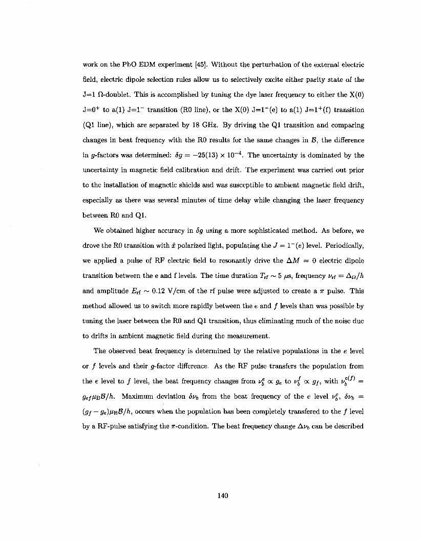
work on the PbO EDM experiment [45]. Without the perturbation of the external electric
field, electric dipole selection rules allow us to selectively excite either parity state of the
J = l fi-doublet. This is accomplished by tuning the dye laser frequency to either the X(0)
J=0+ to a(l) J= l~ transition (RO line), or the X(0) J=l~(e) to a(l) J=l+(f) transition
(Ql line), which are separated by 18 GHz. By driving the Ql transition and comparing
changes in beat frequency with the RO results for the same changes in B, the difference
in p-factors was determined: Sg = —25(13) x 10 - 4 . The uncertainty is dominated by the
uncertainty in magnetic field calibration and drift. The experiment was carried out prior
to the installation of magnetic shields and was susceptible to ambient magnetic field drift,
especially as there was several minutes of time delay while changing the laser frequency
between RO and Ql.
We obtained higher accuracy in Sg using a more sophisticated method. As before, we
drove the RO transition with x polarized light, populating the J = 1~ (e) level. Periodically,
we applied a pulse of RF electric field to resonantly drive the AM = 0 electric dipole
transition between the e and f levels. The time duration Trf ~ 5 /is, frequency i/rf = Au/h
and amplitude Erf ~ 0.12 V/cm of the rf pulse were adjusted to create a IT pulse. This
method allowed us to switch more rapidly between the e and / levels than was possible by
tuning the laser between the RO and Ql transition, thus eliminating much of the noise due
to drifts in ambient magnetic field during the measurement.
The observed beat frequency is determined by the relative populations in the e level
or / levels and their gf-factor difference. As the RF pulse transfers the population from
the e level to / level, the beat frequency changes from v% tx ge to J/J| OC gf, with v"^*' =
geffi^B/h. Maximum deviation Sui, from the beat frequency of the e level v%, Sv^ =
{9f ~ 9e)^B/h, occurs when the population has been completely transfered to the / level
by a RF-pulse satisfying the 7r-condition. The beat frequency change Ai^ can be described
140
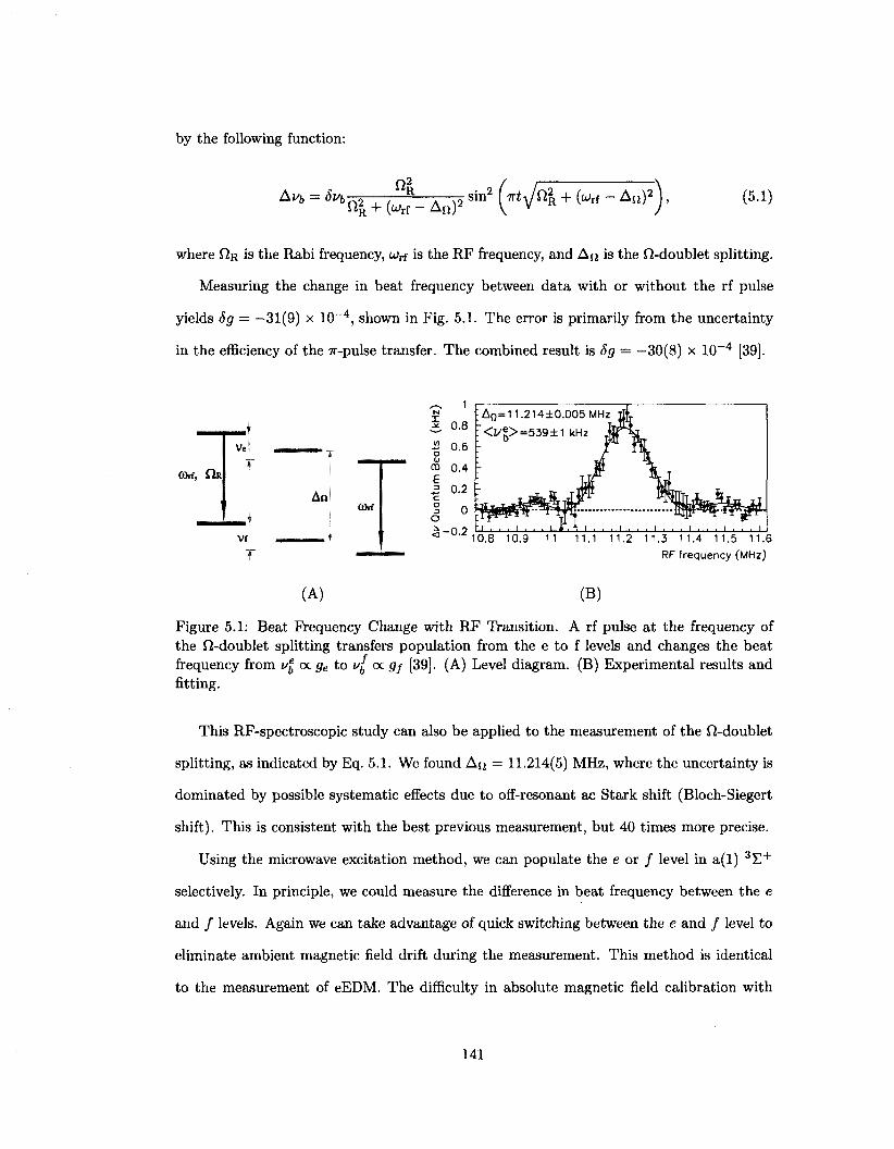
by the following function:
Al/b = 'X+(^-A„)» sin2 ( W ^ + ^ - A « ) a ) • c5-1) where QR is the Rabi frequency, wrf is the RF frequency, and AJJ is the fi-doublet splitting.
Measuring the change in beat frequency between data with or without the rf pulse
yields 8g = —31(9) x 10 - 4 , shown in Fig. 5.1. The error is primarily from the uncertainty
in the efficiency of the 7r-pulse transfer. The combined result is 5g — —30(8) x 10 - 4 [39].
(Brf, Qld
Vei
An 0)rf
Vf
1
0.8
-!2 0.6 o CD
CD 0 .4
A0=11-214±0.005MHz ^
<2/g> = 539±1 kHz
10.8 10.9 11.1 11.2 11.3 11.4 11.5 11.6 RF frequency (MHz)
(A) (B)
Figure 5.1: Beat Frequency Change with RF Transition. A rf pulse at the frequency of the fi-doublet splitting transfers population from the e to f levels and changes the beat frequency from v^ oc ge to u^ oc <?/ [39]. (A) Level diagram. (B) Experimental results and fitting.
This RF-spectroscopic study can also be applied to the measurement of the fi-doublet
splitting, as indicated by Eq. 5.1. We found AJJ = 11.214(5) MHz, where the uncertainty is
dominated by possible systematic effects due to off-resonant ac Stark shift (Bloch-Siegert
shift). This is consistent with the best previous measurement, but 40 times more precise.
Using the microwave excitation method, we can populate the e or / level in a(l) 3 S +
selectively. In principle, we could measure the difference in beat frequency between the e
and / levels. Again we can take advantage of quick switching between the e and / level to
eliminate ambient magnetic field drift during the measurement. This method is identical
to the measurement of eEDM. The difficulty in absolute magnetic field calibration with
141
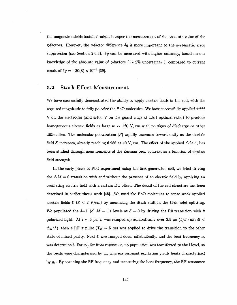
the magnetic shields installed might hamper the measurement of the absolute value of the
g-factors. However, the p-factor difference Sg is more important to the systematic error
suppression (see Section 2.6.3). Sg can be measured with higher accuracy, based on our
knowledge of the absolute value of g-factors ( ~ 2% uncertainty ), compared to current
result of Sg = -30(8) x 10~4 [39].
5.2 Stark Effect Measurement
We have successfully demonstrated the ability to apply electric fields in the cell, with the
required magnitude to fully polarize the PbO molecules. We have successfully applied ±222
V on the electrodes (and ±400 V on the guard rings at 1.8:1 optimal ratio) to produce
homogeneous electric fields as large as ~ 120 V/cm with no signs of discharge or other
difficulties. The molecular polarization \P\ rapidly increases toward unity as the electric
field £ increases, already reaching 0.986 at 40 V/cm. The effect of the applied £-field, has
been studied through measurements of the Zeeman beat contrast as a function of electric
field strength.
In the early phase of PbO experiment using the first generation cell, we tried driving
the AM = 0 transition with and without the presence of an electric field by applying an
oscillating electric field with a certain DC offset. The detail of the cell structure has been
described in earlier thesis work [45]. We used the PbO molecules to sense weak applied
electric fields £ (£ < 2 V/cm) by measuring the Stark shift in the fi-doublet splitting.
We populated the J=l~(e) M = ±1 levels at £ = 0 by driving the R0 transition with x
polarized light. At t ~ 5 //s, £ was ramped up adiabatically over 2.5 /xs ( l /£ • d£/dt <
An/h), then a RF IT pulse (Trf = 5 fxs) was applied to drive the transition to the other
state of mixed parity. Next £ was ramped down adiabatically, and the beat frequency v\,
was determined. For vrf far from resonance, no population was transferred to the f level, so
the beats were characterized by ge, whereas resonant excitation yields beats characterized
by gf. By scanning the RF frequency and measuring the beat frequency, the RF resonance
142
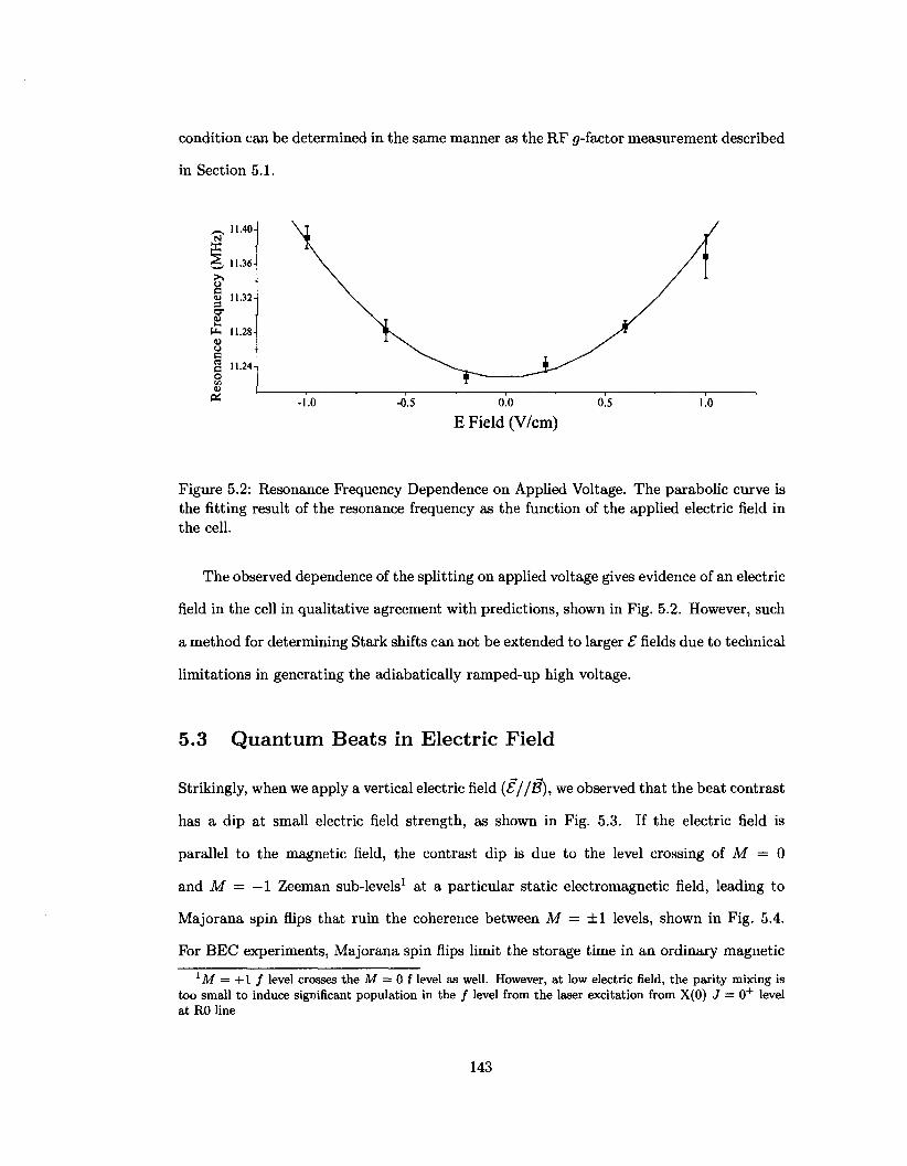
condition can be determined in the same manner as the RF (/-factor measurement described
in Section 5.1.
1.40
11.36
N X
o § 11.32
U- 11.28 u u e 11.24
u 1.0 -0.5 0.0
E Field (V/cm) 0.5 1.0
Figure 5.2: Resonance Frequency Dependence on Applied Voltage. The parabolic curve is the fitting result of the resonance frequency as the function of the applied electric field in the cell.
The observed dependence of the splitting on applied voltage gives evidence of an electric
field in the cell in qualitative agreement with predictions, shown in Fig. 5.2. However, such
a method for determining Stark shifts can not be extended to larger £ fields due to technical
limitations in generating the adiabatically ramped-up high voltage.
5.3 Quantum Beats in Electric Field
Strikingly, when we apply a vertical electric field (S//B), we observed that the beat contrast
has a dip at small electric field strength, as shown in Fig. 5.3. If the electric field is
parallel to the magnetic field, the contrast dip is due to the level crossing of M = 0
and M — —\ Zeeman sub-levels1 at a particular static electromagnetic field, leading to
Majorana spin flips that ruin the coherence between M = ±1 levels, shown in Fig. 5.4.
For BEC experiments, Majorana spin flips limit the storage time in an ordinary magnetic 1M = +1 f level crosses the M = 0 f level as well. However, at low electric field, the parity mixing is
too small to induce significant population in the / level from the laser excitation from X(0) J = 0+ level at R0 line
143
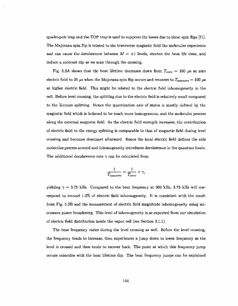
quadrupole trap and the TOP trap is used to suppress the losses due to these spin flips [71].
The Majorana spin flip is related to the transverse magnetic field the molecules experience
and can cause the decoherence between M = ±1 levels, shorten the beat life time, and
induce a contrast dip as we scan through the crossing.
Fig. 5.3A shows that the beat lifetime decreases down from Tzero = 160 /xs at zero
electric field to 20 /is when the Majorana spin flip occurs and recovers to Tnonzero = 100 /is
at higher electric field. This might be related to the electric field inhomogeneity in the
cell. Before level crossing, the splitting due to the electric field is relatively small compared
to the Zeeman splitting. Hence the quantization axis of states is mostly defined by the
magnetic field which is believed to be much more homogeneous, and the molecules precess
along the external magnetic field. As the electric field strength increases, the contribution
of electric field to the energy splitting is comparable to that of magnetic field during level
crossing and becomes dominant afterward. Hence the local electric field defines the axis
molecules precess around and inhomogeneity introduces decoherence in the quantum beats.
The additional decoherence rate 7 can be calculated from
1 1
nonzero •*• zero
yielding 7 = 3.75 kHz. Compared to the beat frequency at 300 kHz, 3.75 kHz will cor
respond to around 1.3% of electric field inhomogeneity. It is consistent with the result
from Fig. 5.3B and the measurement of electric field magnitude inhomogeneity using mi
crowave power broadening. This level of inhomogeneity is as expected from our simulation
of electric field distribution inside the vapor cell (see Section 3.1.1).
The beat frequency varies during the level crossing as well. Before the level crossing,
the frequency tends to increase, then experiences a jump down to lower frequency as the
level is crossed and then tends to recover back. The point at which this frequency jump
occurs coincides with the beat lifetime dip. The beat frequency jumps can be explained
144
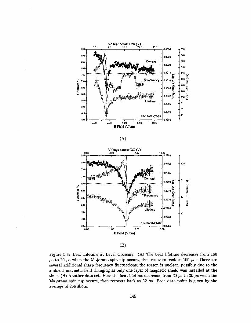
9.0-
8.5-
8.0-
7.5-
^ 7.0-
£ 6.5-
§ O 6.0-
5.5-
5.0-
4.5-
4.0-
0.0
Hfei £P
EM i i 1
\ % \
\
\ , , —,
Voltage across Cell (V) 7.6 15.2 22.9 30.5
i • i • i • i
J E j ^ a , Contrast
1 J t /Frequency -
A I-- mT,ffr*ltth£6:Mitt p. 'XJV'dsPwT^M^'^Vi ^1-' ' J O T Lifetime
T
'•' 16-11-02-02-07 •'"i ' — i • — i ' — i —
0.3030
0.3025
0.3020
0.3015
0.3010
0.3005
0.3000
0.2995
0.2990
0.2985
-i
N X .
>> -a •
9
s . u.
-
260
240
220
200
180 _ tn S
160 w
<a
140-5
120 3
100 « CQ
80
60
40
0.00 2.00 4.00 6.00 E Field (V/cm)
8.00
(A)
Voltage across Cell (V) 3.81 7.62
19-50-08-21-07
0.2965
0.2960
0.2955
60
CQ
E Field (V/cm)
(B)
Figure 5.3: Beat Lifetime at Level Crossing. (A) The beat lifetime decreases from 160 jus to 20 fis when the Majorana spin flip occurs, then recovers back to 100 fj,s. There are several additional sharp frequency fluctuations; the reason is unclear, possibly due to the ambient magnetic field changing as only one layer of magnetic shield was installed at the time. (B) Another data set. Here the beat lifetime decreases from 60 /is to 30 /is when the Majorana spin flip occurs, then recovers back to 52 /is. Each data point is given by the average of 256 shots.
145
A
_1 E=0,8=2gnB aE2»gnB aE2»gnB
Figure 5.4: J = l Level Crossing in Electric Field. (A) The Zeeman effect in zero electric field, where the quantum beat frequency is 2g\isB. (B) Level crossing occurs when the Stark shift is equal to the Zeeman shift, a£2 « g^BB. B\_ is the transverse magnetic field. (C) Level diagram if the Stark shift is much larger than the Zeeman shift.
by the perturbation from the transverse magnetic field Bj_,
where a = /ia/(4An) is the scale factor to describe the quadratic Stark effect. The deriva
tion of Eq. 5.2 is similar to that of Eq. 2.15 in Section 2.6.1. The level crossing occurs at the
electric field 6 = ^Agfj,BB\\An/\ia. Before level crossing, the denominator of the second
term in Eq. 5.2 is positive, so the frequency tends to increase. It experiences a jump down
to lower frequency as the level is crossed and tends to recover back at higher fields. Due
to the electric field inhomogeneity, the curve of the beat frequency versus electric field is
the convolution of Eq. 5.2 and the electric field spread. Notice Eq. 5.2 is only valid asymp
totically when gfiB^x is much less than the level spacing, i.e., before and after the level
crossing. In the limitating case, at high electric field, the perturbation from the transverse
magnetic field is highly suppressed, as discussed in Section 2.6.1. The experimental results
presented here were taken with a single layer of magnetic shield installed, without further
trimming of the transverse magnetic field after degaussing of the magnetic shields. The
transverse magnetic field here can originate from the static magnetic field inhomogeneity,
2 + (g»BB±y (9mB\\? ~ («£2)2 (5.2)
146
the motional magnetic field (see Section 2.6.1), ambient field residual, and the electric field
directional inhomogeneity. With the aid of the cosine-distributed magnetic coils and multi
layers magnetic shields (see Section 3.6), we can have better control on the magnetic field
distribution and noise, and the interesting phenomena during the level crossing can serve
as a nice tool to diagnose the electric field directional inhomogeneity and the systematic
effects due to the transverse magnetic field.
As the electric field increases, the beat amplitude changes in rather a complicated
pattern, shown in Fig. 5.5. With direct horizontal laser excitation, the mixing of e and /
components will lead to population in both. The observed quantum beats will be average
fluorescence signals from both components, which have slightly different beat frequencies
due to the ^-factor difference (discussed later). There are several effects, as discussed below,
which will influence the observed beat amplitude.
At zero electric field, the J = 1~ e component can decay to the ground state X(0)
J = 0 + and J = 2+ , following parity selection rules. There two decay channels have beat
contrast of at 100% and 7.7%. Because of the lack of knowledge of the branching ratio
between the decay channels, the combined beat constrast can range from 7.7% to 100%.
After the level crossing, the beat amplitude does not recover to its initial amplitude at
zero electric field. It may be explained by the mixing of different parity levels in a(l) f2-
doublets which will increase the number of decay channels. The induced even-parity J = l
/ component decays into the ground state X(0) J = 1" level, as the parity of the X(0) J
level is (—1)J. This decay channel has contrast of 33%. Higher electric fields induce more
of the J = 1 / component, but the effect on the beat amplitude depends on the branching
ratio to each decay channel. If the decay to X(0) J = 0+ is the dominant channel, the
intrinsic contrast at zero electric field will be larger than 33%, and the introduction of the
J = 1 / component with lower beat contrast decreases the beat contrast, otherwise, the
contrast increases. To see this point, let us consider one situation: the horizontal polarized
laser drives the R0 transition and excites the molecules from the ground state X(0) J = 0
to the excited state a(l) 3 S + J = 1 in the presence of the external electric field £ = Ez and
147
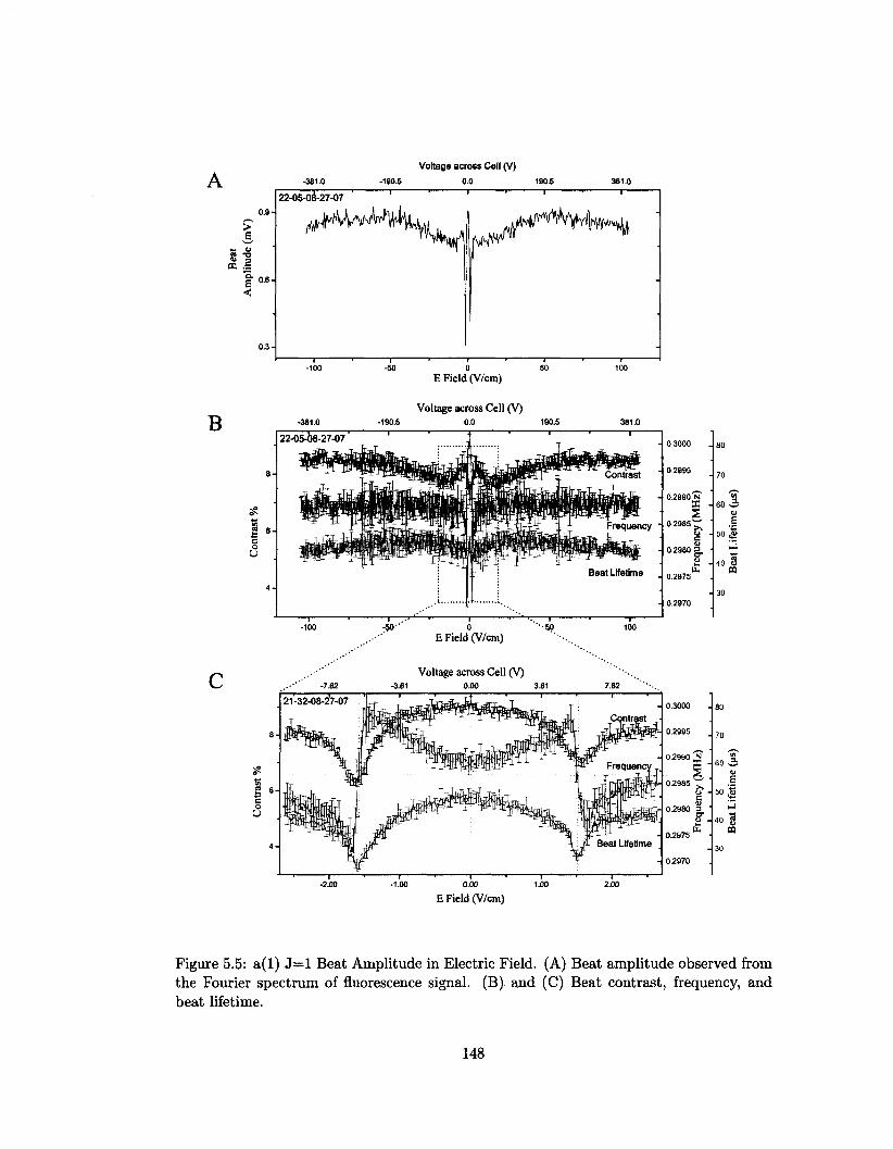
•i 0.9-
0.6-
0.3-
-381.0
22-05-08-27-07
-190.5
wW^i
Voltage across Cell (V)
0.0
frfX r
190.5
4i>rt#iy,
381.0
+ W ^
-
£ • a a U
E Field (V/cm)
Voltage across Cell (V) -190.5 0.0 190.5 381.0
22-05-68-27-07'
JfaA,ii|p-iy •(P^ffll
_-., ,
r •" >
fejjj llPpf flH^flpiSlUfti ^P^ffP™wl|B ,.
i — , — ^ - , — .
, , „ , ,
Hyijjff)Lr-*ii* L ^ ™
fir - J J
i i
T • ' '..—r~
« T
Contrast
•'• Frequency •
wkklj& Jki.^ f wWnpf^Hr
Beat Lifetime
• - i
0.3000
0.2995
0.2990 N X
s 0 . 2 9 8 5 ^
S1
0.2975
0.2970
70
<-\ 60 3
.6 so «g
'•3
40 U 01
-50" E Field (V/cm)
•50
£ 6
21-32-08-2'7-07 1
Voltage across Cell (V) -3.81 0.00 3.81 7.62
60 w u E
50 t>
-to gj m
E Field (V/cm)
Figure 5.5: a(l) J = l Beat Amplitude in Electric Field. (A) Beat amplitude observed from the Fourier spectrum of fluorescence signal. (B) and (C) Beat contrast, frequency, and beat lifetime.
148
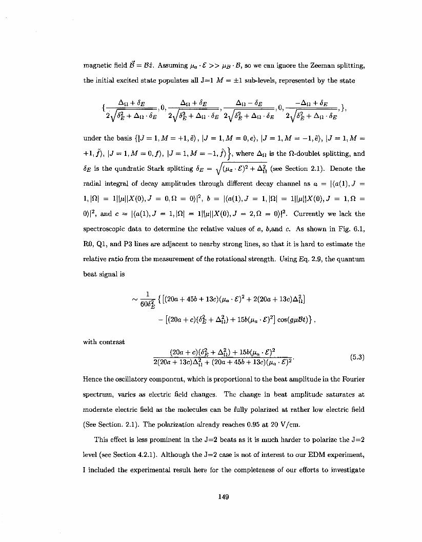
magnetic field B = Bz. Assuming fxa • £ » HB • B, so we can ignore the Zeeman splitting,
the initial excited state populates all J = l M = ±1 sub-levels, represented by the state
A;; + 8E An + 5E An - 8E - A n + 5E ,
2yfg2E +An-SE ' 2y/52
E +An-5^2^/51 + An-6E ' 2y/s2E + A» • SE '
under the basis {\J = 1,M = + l , e ) , \J = l ,M = 0,e>, \J = 1,M = - l , e ) , | J = l , M =
+1, / ) , | J = 1, M = 0, / ) , | J = 1, M = - 1 , / ) I, where An is the fi-doublet splitting, and
SE is the quadratic Stark splitting SE = •v/(/ a • £)2 + A u (see Section 2.1). Denote the
radial integral of decay amplitudes through different decay channel as a = |(a(l), J =
i,|fi| = i|H|x(o),J = o,n = o)|2, b = \{a(i),j = i,|n| = i||HI^(o),J = i,n =
0)|2, and c = | (a(l) ,J = 1,|0| = l\\fj,\\X(0),J = 2,0. = 0)|2. Currently we lack the
spectroscopic data to determine the relative values of a, 6,and c. As shown in Fig. 6.1,
R0, Ql, and P3 lines are adjacent to nearby strong lines, so that it is hard to estimate the
relative ratio from the measurement of the rotational strength. Using Eq. 2.9, the quantum
beat signal is
~ o^2" ([(20a + 45b + 13c)^« • 5 ) 2 + 2(20a + 13c)An] E
- [(20a + c){8% + An) + 15&(/*« • £)2} cos{g^Bt)} ,
with contrast
(20a + c ) ( 4 + A2) + 156(Ma • £? (5.3)
2(20a + 13c)An + (20a + 456 + 13c)(jia • £)2'
Hence the oscillatory component, which is proportional to the beat amplitude in the Fourier
spectrum, varies as electric field changes. The change in beat amplitude saturates at
moderate electric field as the molecules can be fully polarized at rather low electric field
(See Section. 2.1). The polarization already reaches 0.95 at 20 V/cm.
This effect is less prominent in the J=2 beats as it is much harder to polarize the 3—2
level (see Section 4.2.1). Although the J=2 case is not of interest to our EDM experiment,
I included the experimental result here for the completeness of our efforts to investigate
149
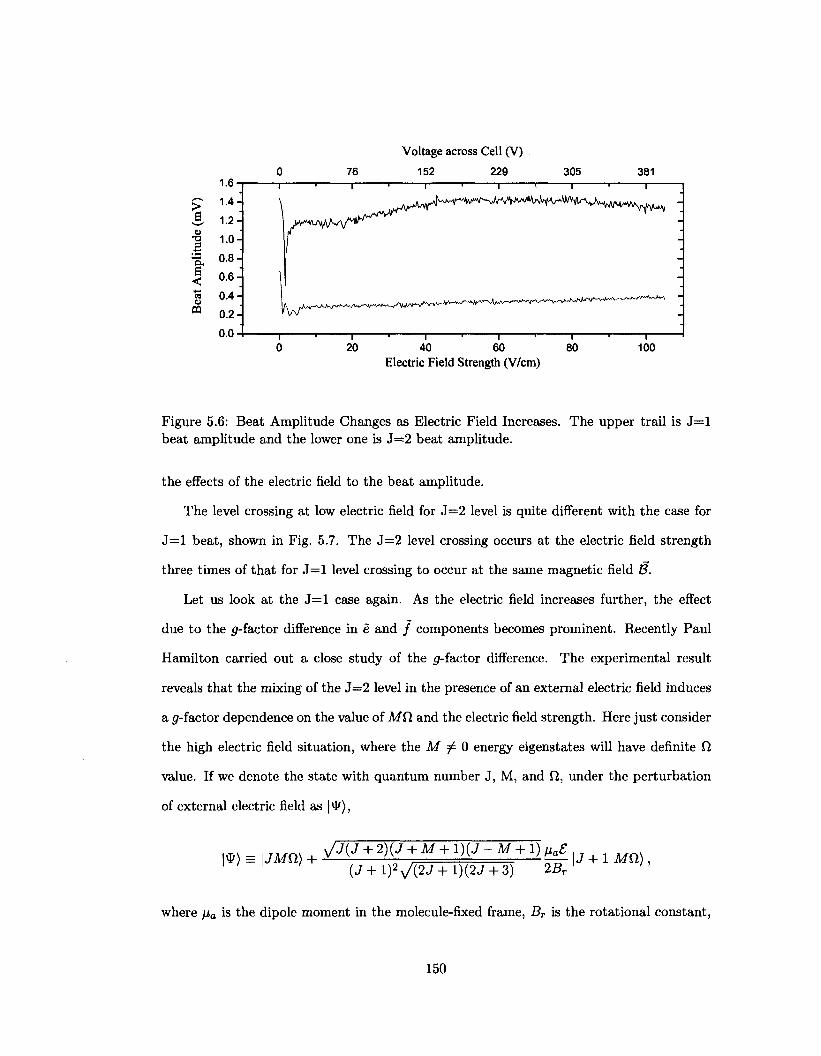
I u
s I < o
Voltage across Cell (V) 152 229
20 -I • 1-
40 60 Electric Field Strength (V/cm)
Figure 5.6: Beat Amplitude Changes as Electric Field Increases. The upper trail is J = l beat amplitude and the lower one is J=2 beat amplitude.
the effects of the electric field to the beat amplitude.
The level crossing at low electric field for J=2 level is quite different with the case for
J = l beat, shown in Fig. 5.7. The J=2 level crossing occurs at the electric field strength
three times of that for J = l level crossing to occur at the same magnetic field B.
Let us look at the J = l case again. As the electric field increases further, the effect
due to the p-factor difference in e and / components becomes prominent. Recently Paul
Hamilton carried out a close study of the g-faetor difference. The experimental result
reveals that the mixing of the J=2 level in the presence of an external electric field induces
a p-factor dependence on the value of Mfi and the electric field strength. Here just consider
the high electric field situation, where the M •£ 0 energy eigenstates will have definite fi
value. If we denote the state with quantum number J, M, and fi, under the perturbation
of external electric field as |\&),
1 / 1 ' (J + l ) V ( 2 . / + l)(2J + 3) 2Br] '
where fj,a is the dipole moment in the molecule-fixed frame, Br is the rotational constant,
150
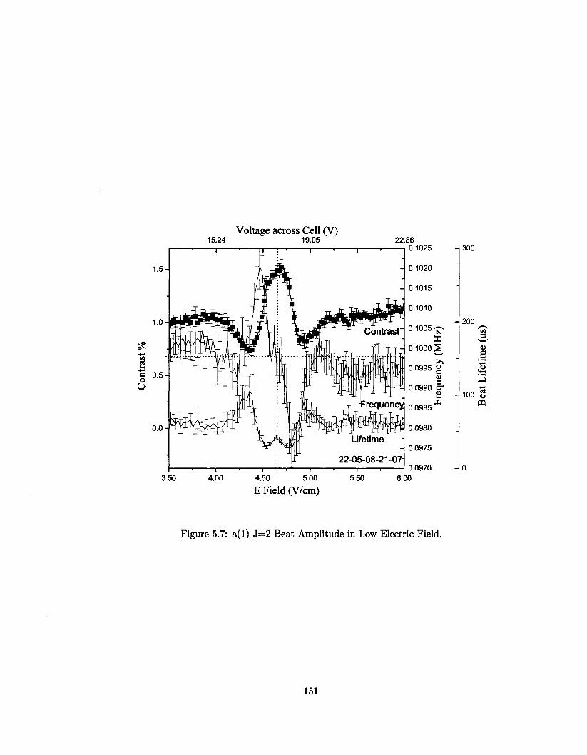
Voltage across Cell (V) 15.24 19.05
— i ' p—r~> 1 f -22.86
0.1025
Lifetime
22-05-08-21-07-
3.50 4.00 4.50 5.00
E Field (V/cm)
i 5.50
0.0985
0.0980
0.0975
0.0970 6.00
Figure 5.7: a(l) J=2 Beat Amplitude in Low Electric Field.
151
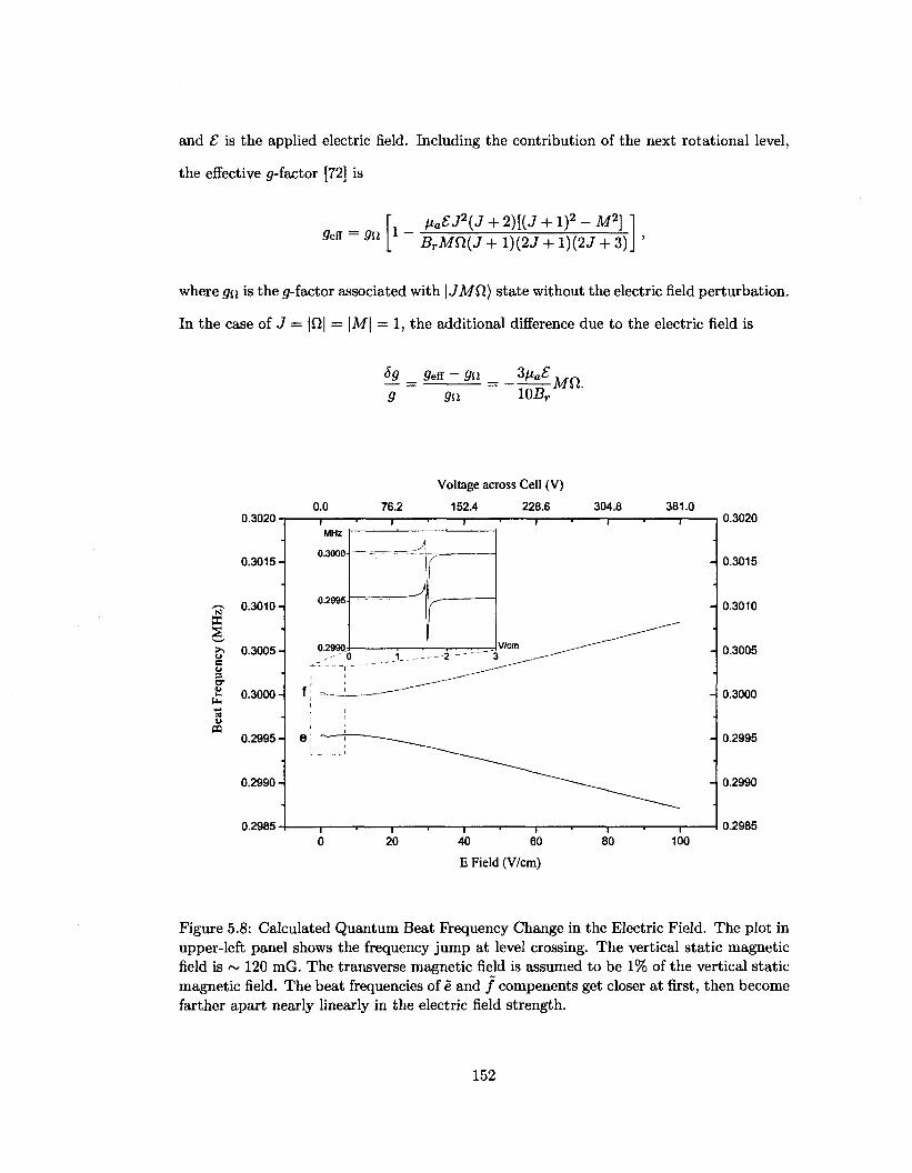
and £ is the applied electric field. Including the contribution of the next rotational level,
the effective ff-factor [72] is
9eS = 9n M a gJ 2 ( J + 2)[(J + l ) 2 - M 2 ]
BrMQ.{J + 1)(2J + 1)(2J + 3)
where gu is the g-factor associated with | JMfi) state without the electric field perturbation.
In the case o f J = |fi| = \M\ = 1, the additional difference due to the electric field is
^R — 9efl ~ 9ii - _ ^ £ g gu 10Br
Mn.
QJ
pa
0.3020
0.3015 H
- 0.3010.
^ 0.3005-s u §• o 0.3000 •
0.2995 H e
0.2990
0.2985
0.0
MHz
0.3000+
0.2995-T
0.2990
76.2
Voltage across Cell (V) 152.4 228.6 304.8
V/cm
20 40 60
E Field (V/cm)
T
80
381.0
100
0.3020
-4 0.3015
0.3010
0.3005
0.3000
0.2995
H 0.2990
0.2985
Figure 5.8: Calculated Quantum Beat Frequency Change in the Electric Field. The plot in upper-left panel shows the frequency jump at level crossing. The vertical static magnetic field is ~ 120 mG. The transverse magnetic field is assumed to be 1% of the vertical static magnetic field. The beat frequencies of e and / compenents get closer at first, then become farther apart nearly linearly in the electric field strength.
152
This effect, at high electric field, yields an additional g-factor difference between the e
and / components, compared to the intrinsic difference in absence of electric field, shown
in Fig. 5.8. As nominally /j.a£ ~ 50 MHz at the electric field strength ~ 70 V/cm, Br ~
14 GHz, the (/-factor difference 5g between e and f component will be 1% of the average
e?-factor. In the e component of fi-doublet states where M£l = 1, the beat frequency of
M = ±1 Zeeman sublevels decreases by -§§}—• In the / component where MQ, — — 1,
the beat frequency increases by the same amount. Thus the average frequency remain
unchanged, as shown in Fig.5.5B. In high magnetic field B and electric field, the beat
frequency splitting due to the different g-factors can be resolved by studying the Fourier
spectrum of the quantum beat with the laser horizontally polarized and tuned to the
R0 line, populating both of fi-doublet levels. The interference between these two close
frequencies generates apparent lifetime shortening and spectral line broadening, as shown
in Fig. 5.9. This effect might be part of the reasons that the observed beat amplitude
decreases at high electric fields.
For a large frequency difference, as we increase the electric field, the beat amplitudes
will have nodes and anti-nodes during the lifetime period, shown in Fig. 5.9. The frequency
difference can be determined by the time span Tn between the laser shot and the node,
8u> = ir/Tn. The data analysis by Paul Hamilton has shown that the beat frequency
difference dependence on the electric field matches the prediction of theory very well.
Another effect that influences the observed beat amplitude is a technical issue related
to the windowing in signal process. As mentioned, we monitor the beat amplitude in
the Fourier spectrum. Typically, a Blackman window is applied. A simulation by Paul
Hamilton demonstrated that the application of a window function in the presence of two
closely spaced frequency components modulates the averaged amplitude depending on the
frequency difference, with an amplitude peak at a certain frequency difference. The sepa
ration of these two peaks in the windowed Fourier transform are not exactly equal to the
actual frequency difference. This effect really complicate the dependence of the observed
beat amplitude in the electric field. Further quantitative investigation is needed to clarify
153
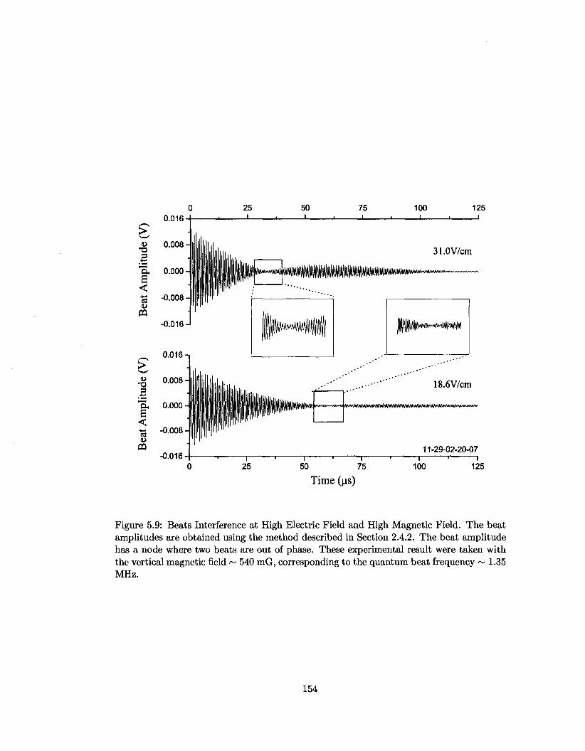
25 50 0.016'
u 0.008 •
0.016-n
.g 0.008-||
75 100 125 i
31.0V/cm
18.6V/cm
JMt+**A*r^^**^mw^^
75 —r -
100
11-29-02-20-07 • 1
125
Time (|xs)
Figure 5.9: Beats Interference at High Electric Field and High Magnetic Field. The beat amplitudes are obtained using the method described in Section 2.4.2. The beat amplitude has a node where two beats are out of phase. These experimental result were taken with the vertical magnetic field ~ 540 mG, corresponding to the quantum beat frequency ~ 1.35 MHz.
154
this effect.
The above discussion cannot explain the relation between the beat amplitude and the
electric field quantitatively. Further experiments and data analysis will be carried out to
bring more insight into the effects of the electric field.
5.4 Conclusion
In conclusion, we improves the precision of the p-factors and molecular electric dipole
moment of the a(l) J = l states based on the improved experimental setup and data fitting
method. Several interesting phenomena of quantum beats in the presence of electric field
have been investigated to provide further insight of our feature-rich molecular structures.
The revelation of the additional p-factors difference induced by the mixing of 3—2 level gives
better quantitative control on the systematic error suppression using fi-doublet comparison.
155
Chapter 6
Current Status and Future
Directions
6.1 Current Status
Various attempts have been taken to optimize the excitation efficiency and detection ef
ficiency of PbO EDM experiment. Several results show that our original estimates were
over-optimistic and the sensitivity of the current setup will be lower than the original
proposed sensitivity by several orders of magnitude.
First, the available signal is much smaller than expected. We have determined that
the partial pressure of PbO vapor is much smaller than the number extrapolated from the
CRC Handbook of Chemistry and Physics [73], which the original proposal is based on.
Recently Paul Hamilton carried out an experiment to measure the microwave absorption
between the J = l and 3=2 rotational states of the ground state X(0) of PbO with vibrational
number v = 1. The experimental results reveal that the observed signal is consistent with a
partial pressure of PbO 10 ~ 50 times smaller than the CRC value. The small fluorescence
signal from excitation of the a(l) [3S+] state also places suspicion on the suitability of
applying the CRC value to our vapor cell configuration. Other papers in the literatures
[74, 75, 76, 77] claim Pb202 and Pb404 are created during the vaporization of PbO, and
156
found the vapor pressure of PbO ranging from 2 ~ 100 times lower than that in the CRC.
Hence, we may have overestimated the density of available PbO molecules by a factor of
~ 30 with the nominal amount of PbO source and heater temperature compared to the
original proposal. A recent study shows that by using more PbO source to increase the
PbO vapor density, the partial pressure of PbO vapor can reach about one tenth of that in
the CRC data. Notice that increasing PbO vapor density will lead to higher collision rate
and decrease the effective state lifetime. Attempts are being taken to study the optimal
vapor pressure and the corresponding heater temperature.
Second, it has been observed that we might be reaching the laser-power saturated region
of laser excitation. This is consistent with our observations that increasing laser power does
not increase the signal to noise significantly. The manufacture's specification of the spectral
width of our pulsed dye laser is about 1 ~ 2 GHz around the lasing frequency, but the
spectral profile at a single laser pulse contains narrow spikes spreading under a broad
envelope, which average to the 1GHz width over many pulses. Individual shots might have
much higher power at certain frequencies, hence the laser excitation will saturate certain
velocity groups of the molecules in the vapor cell. Amplified spontaneous emission (ASE)
from the dye laser contributes significant fluorescent backgrounds to our detection system,
as it causes additional scattered light not resonant with the desired molecular transition and
possibly resonant with adjacent rotational lines in 208PbO by accident (see Fig. 6.1). The
R6 transition of 208PbO is close to the R0 transition, and the fluorescence that it induces is
one of the major backgrounds that reduce the contrast. Recent studies of the laser spectrum
were carried out by scanning the laser frequency and monitoring the J = 1 quantum beat
amplitude. The profile of the fluorescence spectrum can be fitted by a ~1.8 GHz FWHM
central Gaussian peak with lower but broad tails fitted to a Gaussian or Lorentzian profile
with the FWHM ~12 GHz. The Simulation based on these lineshape fit gave a ratio of
0.36 of fluorescence from Ro compared to all other lines for the Gaussian tail fit and 0.24
for the Lorentzian tail fit. Correspondingly, the contrast should be reduced by a factor of
3 ~ 4 from the theoretical contrast of Ro alone. The simulation of the full PbO spectra
157
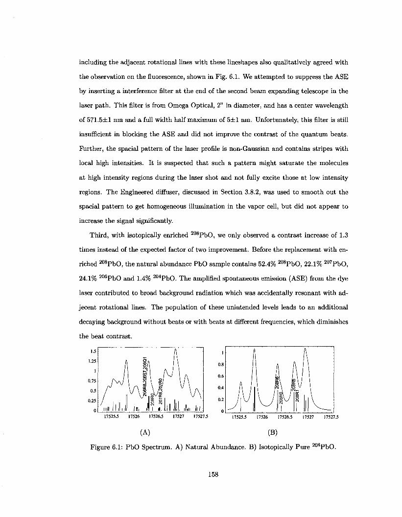
including the adjacent rotational lines with these lineshapes also qualitatively agreed with
the observation on the fluorescence, shown in Fig. 6.1. We attempted to suppress the ASE
by inserting a interference filter at the end of the second beam expanding telescope in the
laser path. This filter is from Omega Optical, 2" in diameter, and has a center wavelength
of 571.5±1 nm and a full width half maximum of 5±1 nm. Unfortunately, this filter is still
insufficient in blocking the ASE and did not improve the contrast of the quantum beats.
Further, the spacial pattern of the laser profile is non-Gaussian and contains stripes with
local high intensities. It is suspected that such a pattern might saturate the molecules
at high intensity regions during the laser shot and not fully excite those at low intensity
regions. The Engineered diffuser, discussed in Section 3.8.2, was used to smooth out the
spacial pattern to get homogeneous illumination in the vapor cell, but did not appear to
increase the signal significantly.
Third, with isotopically enriched 208PbO, we only observed a contrast increase of 1.3
times instead of the expected factor of two improvement. Before the replacement with en
riched 208PbO, the natural abundance PbO sample contains 52.4% 208PbO, 22.1% 207PbO,
24.1% 206PbO and 1.4% 204PbO. The amplified spontaneous emission (ASE) from the dye
laser contributed to broad background radiation which was accidentally resonant with ad-
jecent rotational lines. The population of these unintended levels leads to an additional
decaying background without beats or with beats at different frequencies, which diminishes
the beat contrast.
1.5
1.25
1
0.75
0.5
0.25
n 1 III 1 1 1 , 1 1:1:
587^
2060
.
J — 2
08
37RO
_
'a
8 | | | 1 , I.I II
111, L In 17525.5 17526 17526.5 17527 17527.5 17525.5 17526 17526.5 17527 17527.5
(A) (B)
Figure 6.1: PbO Spectrum. A) Natural Abundance. B) Isotopically Pure 208PbO.
158
Fourth, the excitation efficiency using microwave pulses to transfer the population from
the a(l) J = l M=0 states to the desired EDM state is around 30 ~ 40% at the time of this
thesis work. The imperfect excitation decreases the contrast of the quantum beats by a
factor of 2. With a new microwave amplifier with higher power output, it was expected
to improve the excitation efficiency significantly. There are concerns that the boundary
conditions set by the metallic electrodes might limit the efficiency on the transition driven
by the horizontally polarized microwaves.
Finally, the actual outcome of the detection scheme is less efficient than expected.
Currently the fluorescence is collected by a 2" diameter lightpipe, then passing through an
IR blocking glass, a sapphire window, and two IF filter before hitting the detector. The first
IF filter is a standard IF filter with 50% transmission, 10 nm bandpass, centered at 550 nm.
The second filter is an Omega filter with high transmission (~ 90%) and cut on wavelengths
of 544 nm and 560 nm. This filter is made using Omega's 3 rd Millennium Technology Alpha
Gamma technique, which has higher transmission and a steeper cut-off than a standard
interference filter. The design and experimental study of the filter properties has been
discussed in detail in Ref. [64]. The actual improvement with the Omega filter in place
was less than expected. The reason is still under investigation. We choose Hamamatsu
R329EGP PMTs with 15% q.e. as detectors for the current experimental stage. Although
photodiodes have a much higher quantum efficiency at 550 nm, the current signal size is
too small to take advantage of photodiodes; the signal to noise ratio with photodiodes is
not better than the PMTs in the current background dominated regime, as discussed in
Section 3.8.4. In conclusion, the detection efficiency is estimated to be around 2 x 10 - 4 ,
based on fluorescence collection efficiency 4% (from Monte Carlo simulation), IR filter
transmission 90%, IF filters' transmission 7%, surface loss 42%, and the detector's quantum
efficiency 15%.
Based on the current configuration of the experiment, we can estimate the shot-noise-
limited frequency resolution. At the nominal temperature of the PbO vapor T = 700° C,
the estimated PbO vapor density is about 1.4 x 10 - 4 Torr (including the discrepancy from
159
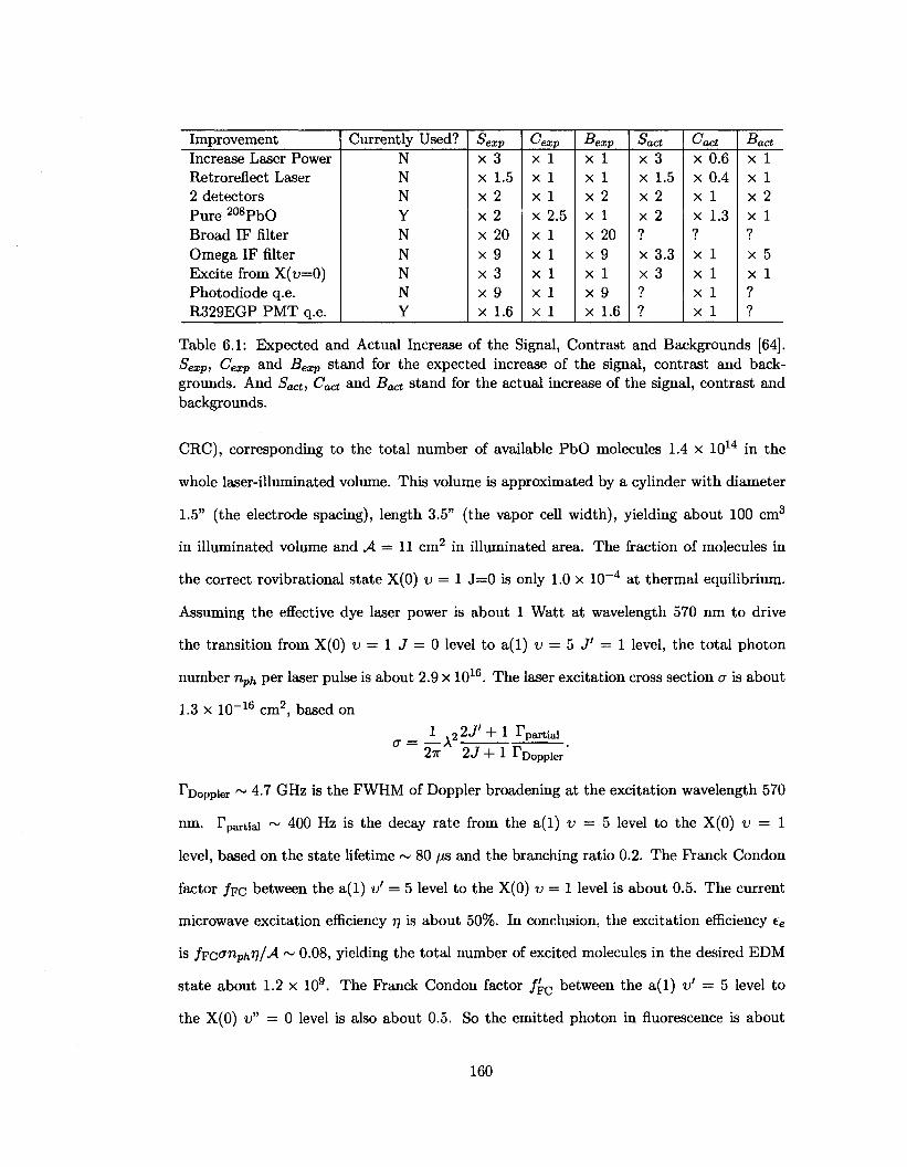
Improvement Increase Laser Power Retroreflect Laser 2 detectors Pure 208PbO Broad IF filter Omega IF filter Excite from X(u=0) Photodiode q.e. R329EGP PMT q.e.
Currently Used? N N N Y N N N N Y
&exp
x 3 x 1.5 x 2 x 2 x 20 x 9 x 3 x 9 x 1.6
(-'exp
X 1
X 1
X 1
x 2.5 x 1 x 1 x 1 x 1 x 1
•tfexp
X 1
X 1
x 2 x 1 x 20 x 9 x 1 x 9 x 1.6
&act
X 3
x 1.5 x 2 x 2 ?
x 3.3 x 3 ?
?
Cacl x 0.6 x 0.4 x 1 x 1.3 ?
x 1 x 1 x 1 x 1
Bad X 1
X 1
X 2
X 1
?
x 5 X 1
?
?
Table 6.1: Expected and Actual Increase of the Signal, Contrast and Backgrounds [64]. Sexpi Cexp and Bexp stand for the expected increase of the signal, contrast and backgrounds. And Sad, Cact and Bact stand for the actual increase of the signal, contrast and backgrounds.
CRC), corresponding to the total number of available PbO molecules 1.4 x 10¹⁴ in the
whole laser-illuminated volume. This volume is approximated by a cylinder with diameter
1.5" (the electrode spacing), length 3.5" (the vapor cell width), yielding about 100 cm3
in illuminated volume and A = 11 cm2 in illuminated area. The fraction of molecules in
the correct rovibrational state X(0) v = 1 J=0 is only 1.0 x 10~4 at thermal equilibrium.
Assuming the effective dye laser power is about 1 Watt at wavelength 570 nm to drive
the transition from X(0) v = 1 J = 0 level to a(l) v = 5 J ' = 1 level, the total photon
number nph per laser pulse is about 2.9 x 10¹⁶. The laser excitation cross section a is about
1.3 x 10"16 cm2, based on
_ 1 .2 2-/ + 1 1 partial
27T 2 J + 1 Tooppler
Tooppier ~ 4.7 GHz is the FWHM of Doppler broadening at the excitation wavelength 570
nm. Tpartiai ~ 400 Hz is the decay rate from the a(l) v = 5 level to the X(0) v = 1
level, based on the state lifetime ~ 80 /xs and the branching ratio 0.2. The Franck Condon
factor /FC between the a(l) v' = 5 level to the X(0) v — 1 level is about 0.5. The current
microwave excitation efficiency r) is about 50%. In conclusion, the excitation efficiency ee
is fFCtrnphV/A ~ 0.08, yielding the total number of excited molecules in the desired EDM
state about 1.2 x 10⁹. The Franck Condon factor / F C between the a(l) v' = 5 level to
the X(0) v" = 0 level is also about 0.5. So the emitted photon in fluorescence is about
160
n/ = 6 x 10⁸ per laser shot. The detection efficiency e is estimated to be around 2 x 10 - 4 .
The laser fires at r = 100 Hz. Hence the counting rate dN/dt ~ re^nf is 1.2 x 10⁷ /s. The
observed contrast is C ~ 3% using the microwave excitation scheme.
The complete formula of frequency resolution per shot using contrast and signal size is
given by Eq. 2.10 (see Section 2.4.2),
s _**VS±B_ 2nS0CT3/2y/2B2'
Currently, the observed a is about 1.6 x 10~2 y/V for a single shot, quantum beat signal
size S ~ 0.1 V, the blackbody background size B ~ 0.2 V, contrast C ~ 3% using the
microwave excitation scheme, the effective lifetime ~ 50 (J,S, and the bandwidth of data
aquisition ~ 2.5 MHz. Hence, the current frequency resolution is ~ 240 HZ/A/HZ. The
corresponded sensitivity to de is only 8 x 10~26e • cm, assuming that EDM data is collected
for 10 days with a 30% duty cycle,.
Although our current sensitivity level is not comparable to the current experimental
limit, it is still worthwhile to carry out the EDM data collection as planned. The ex
perimental setup and techniques are ready. Further investigation will help to understand
possible systematic effects in EDM measurement using paramagnetic molecules and pro
vide hints on the possibility of sensitivity improvement. There have been already several
attempts to improve the sensitivity in the meanwhile. One straight-forward improvement
on the current sensitivity level is to use two PMTs set up on both sides of the chamber to
improve the counting rate by factor two and sensitivity by V2. New heat shield materials
are under investigation, aiming to improve the heating efficiency and lower the blackbody
radiation background. Studying and engineering the laser profile will help to improve
the excitation efficiency. The installation of new microwave amplifier will provide ample
adiabatic following parameter space to optimize the population transfer efficiency.
161
6.2 Future Direction I: Microwave Absorption
The microwave excitation scheme, because of its feature of simplicity and robustness,
aroused great interest among us for further exploration. A next generation of the EDM
experiment using microwave absorption of PbO vapor as the novel detection scheme was
proposed recently. The absorption scheme eliminates the drawbacks of the small solid
angle in the fluorescence detection scheme and the signal size scales up linearly with the
length of absorption path. For near resonance absorption, 100% contrast is expected in
the time-resolved absorption profile. Hence, a promising improvement on the sensitivity of
EDM can be achieved in the microwave absorption scheme.
6.2.1 General Description
Once the PbO molecules are prepared in the desired EDM states, it is possible to detect the
EDM signal by measuring the absorption on a microwave resonant between these states
and a J=2 M=0 level. By analogy to the discussion of quantum beats in Chapter 2,
quantum beats will be seen in time-resolved absorption profile with 100% contrast. The
beat frequency can be extracted from the time-resolved absorption profile. The analogy of
optical absorption in three levels was studied using density matrix approach in Ref. [78,
79]. By changing the frequencies of the microwave preparation beam and the absorption
beam, the beat frequency change between the aligned state and anti-aligned state can be
determined to measure the EDM signal.
6.2.2 Absorption Cross Section
Let's consider the absorption cross section for horizontally polarized microwaves first. In
the limit of complete polarization of the molecules in the external electric field £, we denote
|^o) as one of the EDM states in the external electric field l, and |\&i) as the counterpart
state in microwave absorption, as shown in Fig. 6.2.
1 Here the EDM state anti-aligned with £ is shown. The absorption cross section for the EDM state aligned with £ is identical.
162
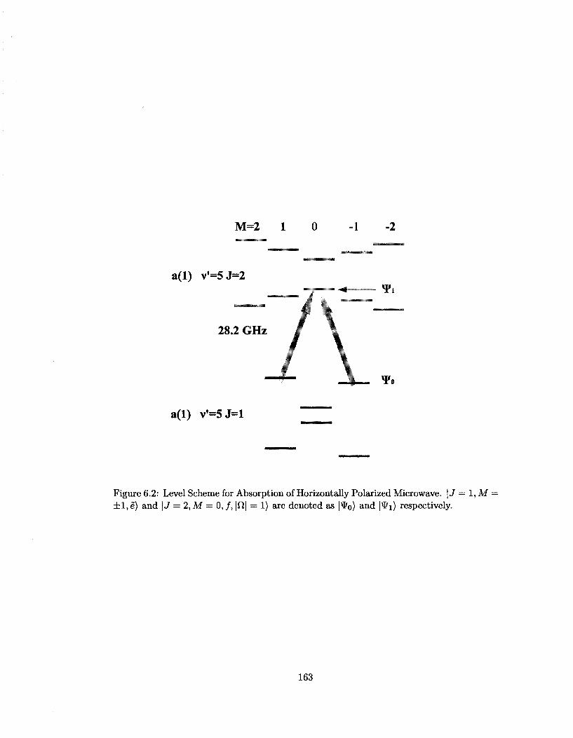
M=2 1 0 •1 -2
a(l) v'=5J=2
28.2 GHz
a(l) v'=5J=l
Figure 6.2: Level Scheme for Absorption of Horizontally Polarized Microwave. \J ±l ,e) and \J = 2,M = 0, / , |fi| = 1) are denoted as |\I/o) and |*i) respectively.
1,M
163
l*o> = \ (I J = 1, M = 1, e, |fi| = 1) - | J = 1, M = 1, /, |ft| = 1))
+ \ ^ 1 (W = 1,M = -1,e, |«| = 1)+|J = 1, M = - 1 , / , \n\ = 1»
= 4= (-1^ = i, Af = i ,n = - i ) + e - i w t | j = I,M = - i , n = i))
v2
|*1> = |J = 2,M = 0,/, |n| = l) = 4=(|J = 2,M = 0,fi = 1) + \J = 2,M = 0,n = -1)),
v2
where u is the angular frequency of the quantum beat.
A straightforward calculation gives an estimate of the absorption cross-section without
Doppler broadening and inhomogeneous broadening,
1 £ 2 I / T i i T M 2 87TI/ 1 . 1 , 2
-abs = ¥^l(*l|^|*0>| 2 = — ^(^a)2
= 9 x 10~13(1 + cosut) cm2.
where $ = g^j;is the photon flux, v is the frequency of microwaves, c is the speed of light,
7 is the natural line width of a(l) J = l state ~ 1/r = 2ir • 3.2 kHz, r is the effective lifetime
~ 50 /is, and na = 3.27 X 10 - 1 8 esu • cm is the molecular dipole moment in CGS units.
The time-resolved absorption depth is modulated at the angular frequency u with contrast
100%.
Molecules have a Maxwell velocity distribution inside the vapor cell, which will induce
Doppler broadening to reduce the absorption cross section. So we must include the effect
of Doppler broadening at the temperature ~ 700° C,
T^ = ^ J 2 ^ = 2TT • 24 kHz,
Moreover, the electric field inhomogeneity in the current cell setup is ^£ ~ 1%. With the
typical value of the DC Stark shift of SE ~ 30MHz, the inhomogeneity-induced broadening
164
IS
TE ~ -j-&E ~ 2TT • 300 kHz,
which is the dominant broadening effect. This reduces the absorption cross section accord
ing to
a « =r-crabs = 10_14(1 + cosatf) cm2. i-E
So the total absorption depth will be
d = rpurl = r\ • 1010cm-3 • 10~14cm2 • 5cm = 5 x 10~V (6.1)
where n ~ 1010 cm - 3 is the estimated density of molecules in the right rovibrational
ground state X(0) J=0 v = 0 accessible by the laser pumping in the current setup, rj is
the efficiency of transferring molecules from that ground state to the desired EDM states,
which is estimated to be around 1 ~ 5% in the current experiment setup, and I is 5 cm for
current vapor cell dimension. In conclusion, the calculation above yields an rough estimate
of the expected absorption depth d for the current setup, of the order ~ 10 - 5 . It is worthy
of notice that the absorption size grows linearly with absorption length if using a longer
cell.
To avoid saturation of absorption requires negligible population transfer between the
resonance levels. Excluding Doppler and electric field inhomogeneity broadening, this gives
a condition on the microwave power
= * « ^ — = l -28x l0- 5 sV/cm 10 flaT c
8TT" =*.£ = £-£2 = 2 x 10~8 W/cm2
=>p = AS = 0.5 /xW,
where (/J,X) = j-7jsMa between I'J'o) and | ^ i ) , S^ is the electric field strength of the mi-
165
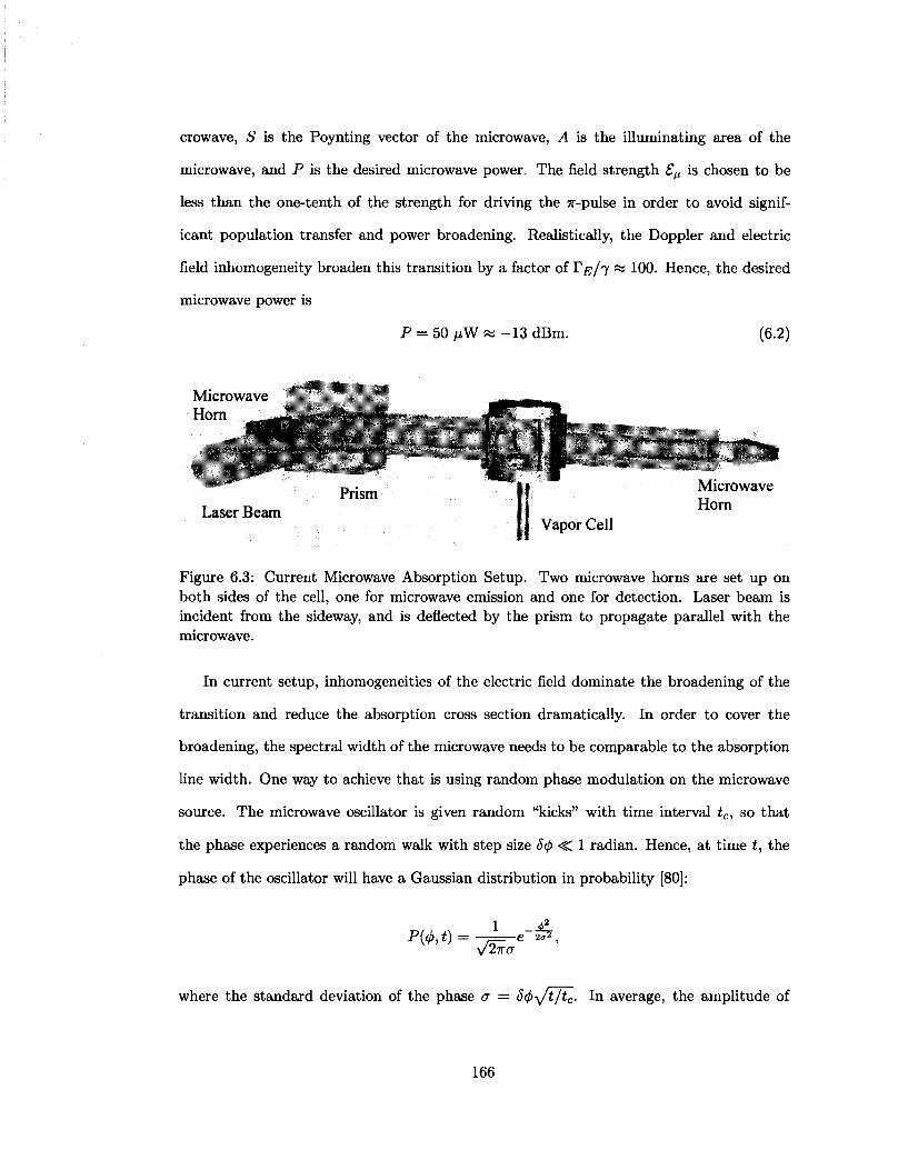
crowave, S is the Poynting vector of the microwave, A is the illuminating area of the
microwave, and P is the desired microwave power. The field strength S^ is chosen to be
less than the one-tenth of the strength for driving the 7r-pulse in order to avoid signif
icant population transfer and power broadening. Realistically, the Doppler and electric
field inhomogeneity broaden this transition by a factor of TE/I « 100. Hence, the desired
microwave power is
P = 50 fiW » -13 dBm. (6.2)
Microwave Horn
Prism Laser Beam
Vapor Cell
Microwave Horn
Figure 6.3: Current Microwave Absorption Setup. Two microwave horns are set up on both sides of the cell, one for microwave emission and one for detection. Laser beam is incident from the sideway, and is deflected by the prism to propagate parallel with the microwave.
In current setup, inhomogeneities of the electric field dominate the broadening of the
transition and reduce the absorption cross section dramatically. In order to cover the
broadening, the spectral width of the microwave needs to be comparable to the absorption
line width. One way to achieve that is using random phase modulation on the microwave
source. The microwave oscillator is given random "kicks" with time interval tc, so that
the phase experiences a random walk with step size 8(j> <C 1 radian. Hence, at time t, the
phase of the oscillator will have a Gaussian distribution in probability [80]:
P(c/>,t) = 1 -£
V2ir> -e to* na
where the standard deviation of the phase a = 5<j)y/t/tc. In average, the amplitude of
166
microwave is proportional to the quantity:
/
OO s ,2t
P{4>,t)eiuiot+'t,d<j> = ei"ot-kr. -OO
The spectral distribution of the microwave is then given by the Lorentzian function
72/4 J(w)oc
(ui — OJQ)2 + 7 2 /4
where 7 = 8(j>2/tc. A reasonable size of 8<j> can be chosen as 0.3, and tc ~ 200 ns, yielding
the broadening of ~ 450 kHz to cover the electric field inhomogeneity-broadened line. In
practice, we can sample a noise source ata 20 ns time interval to give a control voltage
to the phase modulation port of the microwave source with phase modulation amplitude
around 0.1 radian.
Notice that the coupling between |*i) and ^2) = IJ = 2, M = 0, / , |H| = 1) is stronger.
Moreover, the mixing between the M = 0 / and M = 0 e is forbidden, and the mixing
between |^i) and l"^) is suppressed by the rotational level splitting 28.2 GHz. Hence this
coupling is not broadened by the electric field inhomogeneity.
= 1.4 x 10 - 1 1 cm2.
The corresponding absorption depth d is ~ 4 x 10 -3 , assuming the vapor cell length is
5" as current setup. We have carried out a microwave absorption experiment probing
the vertical transition from ^2) to |^i) using the vertically polarized microwave and the
current vapor cell setup. The experimental result confirmed the calculation. We could
monitor the microwave emission from |\I/i) to 1*2) while another microwave beam drives
the population from the EDM states to |* i ) , as shown in Fig. 6.4.
167
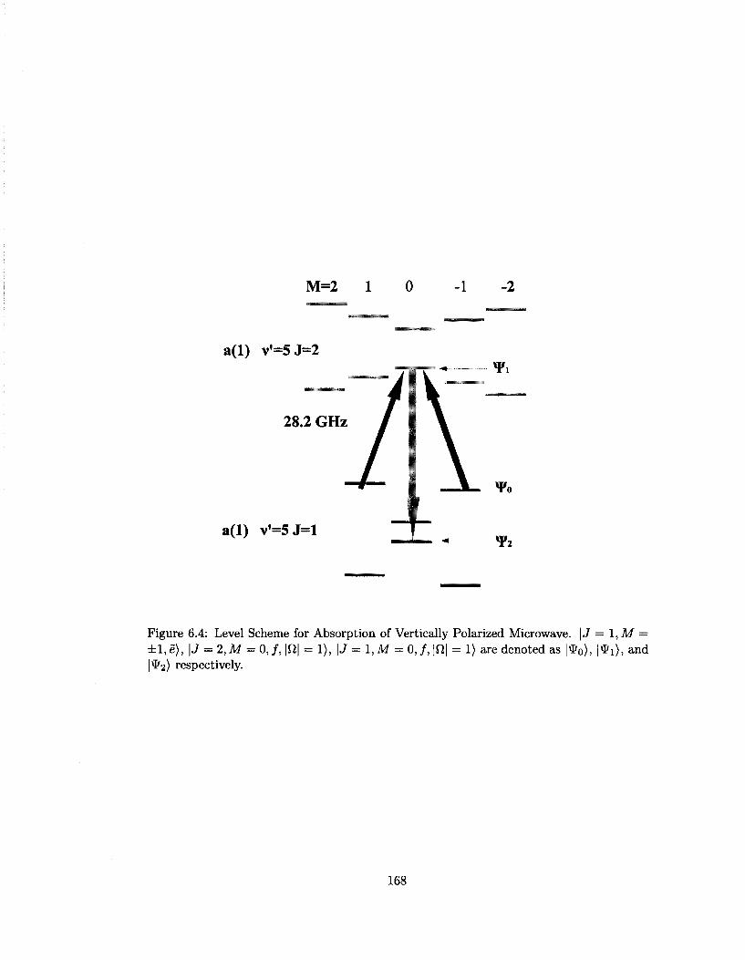
M=2 1 0 •1 -2
a(l) v'=5J=2
28.2 GHz
a(l) v'=5J=l J _ * ^ 2
Figure 6.4: Level Scheme for Absorption of Vertically Polarized Microwave. \J = 1,M = ± l ,e ) , |J = 2,M = 0 , / , |n | = 1), |J = 1,M = 0,/,|12| = 1) are denoted as | * 0 ) , |* i ) , and |VPa) respectively.
168
6.2.3 Signal to Noise
The statistical sensitivity to an EDM will be limited by the signal-to-noise ratio. In the
microwave absorption scheme, the absorption signal will be collected by a microwave horn,
amplified by a microwave amplifier and detected by a square-law detector. The microwave
amplifier noise, treated as thermal noise at the input to the amplifier, will mix with the
microwave signal carrying the absorption signal, and be boosted by the square law detector
to limit the signal-to-noise ratio of the system.
Here we denote the gain of the amplifier G, the thermal noise amplitude of the amplifier
VT, and the microwave signal amplitude V^. The input amplitude to the amplifier, V\n is
the sum of both: V[n = V^ + Vp. The output amplitude of the amplifier is V mp = GV\n,
and it is fed into the square-law detector. The output voltage of the detector will be
proportional to the square of 14mp:
Voat oc G2 (VM + VT)2 OC V2 + 2V^VT + VT2
oc P» + 2^/P^PT + PT
« P„ + 2x / iy^,
where PM is the microwave power of the absorption beam, Pr is the thermal noise power,
and the assumption Pr -C P^ is applied in the last approximation. It is easy to see that
the thermal noise power Pr is boosted by the signal power P^, by the factor 2y /P / i /Pr,
which is large by the assumption Pr -C PM. The thermal noise level of the microwave
amplifier is characterized by the noise figure N, as Pp = kTeffB = k(N - 1)TQB, where
To = 293 K and B « 3 kHz is the bandwidth (determined by the beat effective lifetime r
with 1/27TT « 3 kHz). A typical value for N is 2.8 dB for available low-noise amplifiers. PM
can be estimated based on the output power of microwave source P s (~ 50 /zW in Eq. 6.2)
and transmission loss L before hitting the detector (10 dB in current setup), P^ = PajL.
169
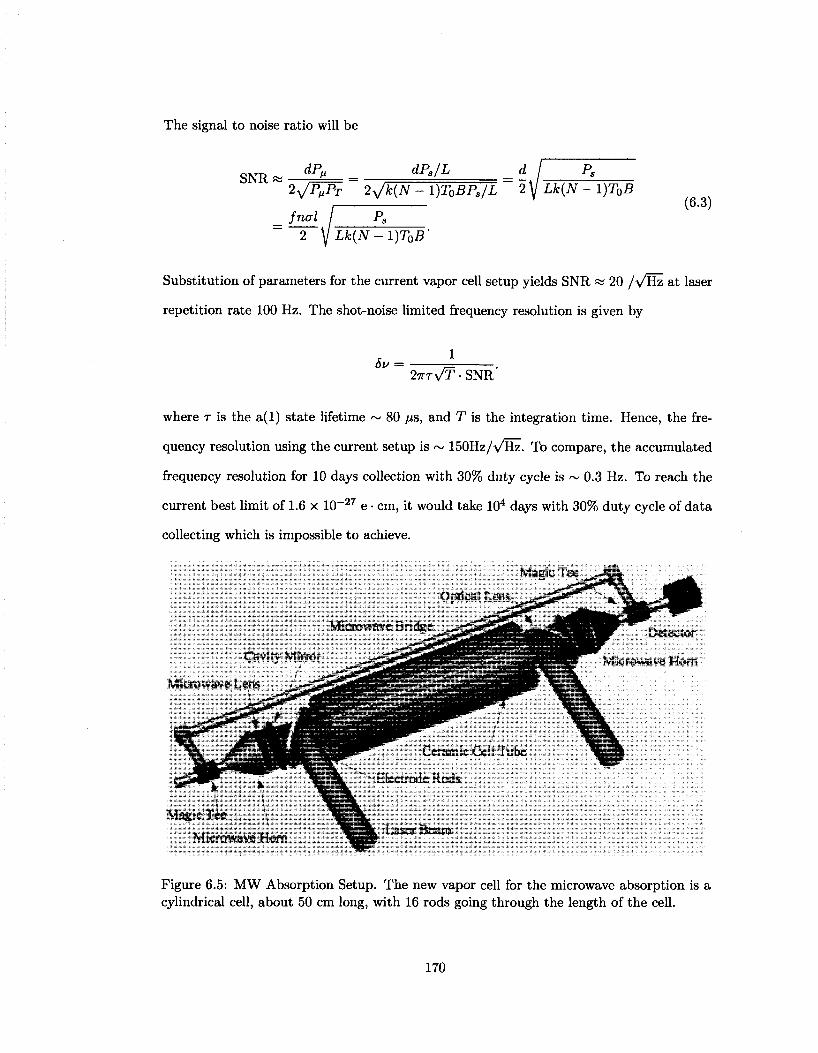
The signal to noise ratio will be
SNRi dP,
a dPs/L
2 ^ / i y V 2y/k{N - 1)TQBPS/L 2 y Lk(N - 1)T0B
fnal I Ps
2 V Lk(N-l)T0B'
(6.3)
Substitution of parameters for the current vapor cell setup yields SNR ss 20 /\/Hz at laser
repetition rate 100 Hz. The shot-noise limited frequency resolution is given by
5u 27nVT-SNR'
where T is the a(l) state lifetime ~ 80 /JS, and T is the integration time. Hence, the fre
quency resolution using the current setup is ~ 150Hz/\/Hz. TO compare, the accumulated
frequency resolution for 10 days collection with 30% duty cycle is ~ 0.3 Hz. To reach the
current best limit of 1.6 x 10~27 e • cm, it would take 104 days with 30% duty cycle of data
collecting which is impossible to achieve.
Magic Tee
Optical Lens s
Microwave Bridge
Microwave Lens
Cavity Mirror /
Magic Tee
Figure 6.5: MW Absorption Setup. The new vapor cell for the microwave absorption is a cylindrical cell, about 50 cm long, with 16 rods going through the length of the cell.
170
However, the calculation shown above is just for the current vapor cell. For the new
proposed setup, the new vapor cell for the microwave absorption (Fig. 6.5) will be a cylin
drical cell, about 50 cm long, with 16 rods going through the length of the cell. These rods
are distributed in a circle with equal spacing, supported by the sapphire windows on the
ends of the cell. Cosine-distributed voltages will be applied on the corresponding rods to
create a homogeneous transverse electric field. Any leakage currents will only flow through
the end windows and have little effect on the main cell volume. The heating elements
for this cell can be tantalum or tungsten wires, which are believed to be much easier to
construct and maintain compared to current oven. The microwave beam is emitted from
the microwave horn with some angular spread and will diverge further as it propagates.
Microwave lenses are used to collimate and focus the microwave beam. A microwave cav
ity is used to increase the absorption path length dramatically, by a factor proportional
to the cavity finesse. All these microwave optics will help to maintain the TEMoo mode
of the microwaves, hence maintaining the microwave polarization and the Gaussian beam
profile. The microwave beam will have small beam width to avoid the perturbation from
the metallic surface of the electrodes. A homodyne interferometer consists of a magic Tee,
bridge, phase delay, and the square-law detector. This setup will diminish the noise due
to amplitude fluctuations of the microwave source.
Many improvements can be carried out to increase the signal to noise ratio of microwave
absorption detection. A long vapor cell will increase the absorption depth proportional to
the transmission length as shown in Eq. 6.1. A 50 cm absorption length will increase
the absorption by a factor of 10. Generating the static electric field by conducting rods
with cosine voltage distribution will improve the electric field homogeneity by the factor
of ~ 10 compared to current cell, which will reduce the inhomogeneous broadening to be
comparable to the Doppler broadening. Better electric field homogeneity will increase the
absorption cross section by 10, but to avoid saturation P s will need to be turned down by
10, and based on Eq. 6.3, this will improve SNR by a factor of \ / l0. A microwave cavity
with finesse F (1,000 feasible) will increase the absorption path length by F, but, similar to
171
electric field homogeneity case, P s will need to be reduced by 1/F, giving an improvement
on SNR by ^1,000 ~ 32. Further improvements include broadening the cavity modes
of the dye laser, using a low-noise cryogenic microwave amplifier, and etc, which could
contribute the improvement by another factor of 100 on the signal to noise.
In conclusion, the ultimate limit to SNR for the microwave absorption scheme is ~
3 x 10⁶ /vTiz per shot, yielding the frequency resolution 0.7 Hz/\/Hz, or a sensitivity of
2 x 10_31e • cm for 10 days of data collecting with 30% duty-cycle at a repetition rate of
100 Hz.
6.3 Future Direction II: Beam EDM
Recently a survey aimed to investigate candidate molecules suitable for a cold beam EDM
experiment was carried out by Amar Vutha [81]. ThO and HfO appear promising for use
in a future cold beam eEDM experiment.
6.3.1 Cold Beam Experiment
Polar molecular systems can provide great enhancement on the EDM sensitivity as the ef
fective internal electric field the electrons experience can be five or more orders of magnitude
higher than the maximal field achievable in the laboratory. Motivated by improvements in
the cold molecule flux from He buffer-gas cells, cold molecular beam experiments for EDM
measurement show great promise.
In a molecular beam frequency measurement, the obtainable frequency resolution is
fo° */L A , (6-4)
where v is the longitudinal velocity of the beam, L is the interaction length, rje, r)d are
the efficiencies for excitation and fluorescence detection respectively, TVo is the molecule
flux from the beam source, ft is the beam divergence solid angle and A is the downstream
172
detection area. Here the dominant noise source is assumed to be Poissonian fluctuations
in the beam flux. In order to take advantage of a molecular beam setup, a coherence
time is required to be at least a few ms. The natural lifetime of PbO a(l) state is only
82/is. Therefore we need to search for new candidates for a cold molecular beam EDM
experiment.
6.3.2 Candidates for Cold Molecular Beam EDM Experiment
Candidates for a cold molecular beam EDM experiment should possess the following fea
tures. First, hetero-nuclear molecules with one atom substantially heavy will take advan
tage of the fact that the EDM enhancement is proportional to Z3. Furthermore, the larger
mass will lead to lower velocity beams from thermalization with the buffer gas. Secondly,
a small ^-doublet splitting is desirable to facilitate the molecular polarization under the
external electric field and to provide an excellent mechanism of systematic effect suppres
sion. Molecules with total symmetry E have been preferred in current molecular EDM
experiments: X 2Ew2 of YbF and a(l) 3E+ of PbO. The unpaired electron in the molecu
lar orbital of a symmetry has no orbital angular momentum about the molecular axis, and
thus can penetrate close to the nucleus of heavy atom, and spend time near the nucleus,
yielding a significant EDM enhancement factor.
Some molecule candidates with nonzero angular momentum about the intra-molecular
axis have been studied in the survey. Molecules of interests will have two valence electrons,
preferably in the a8 molecular orbital configuration. The electron in the a orbital gives an
enhanced EDM signal as discussed before. The electron in the 6 orbital allows the molecule
to possess small Q-doublet splitting. Hence molecules of interest have (aS) 3Au symmetry
overall. Further, the ft = 1 sub-state, 3Ai, has a very small magnetic moment, suppressing
spurious frequency shifts from ambient magnetic fields. Only the molecule TiO (Z=22)
has a 3A ground state, but is too light to be favored for an EDM experiment. TiO-type
molecules, ScF (Z=21), YF (Z=39), ZrO (Z=40), LaF (Z=57), HfO (Z=72), ThO(Z=90),
all have very low lying 3A states arising from the same aS configuration as the 3A state in
173
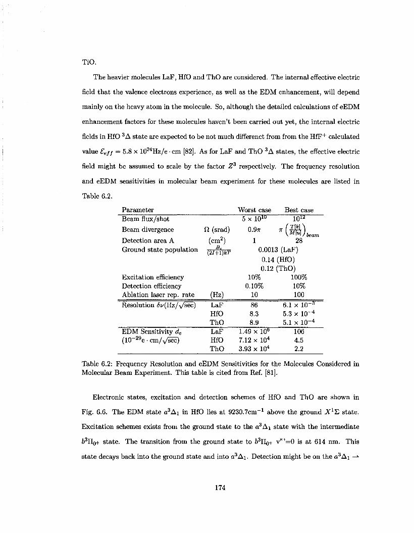
TiO.
The heavier molecules LaF, HfO and ThO are considered. The internal effective electric
field that the valence electrons experience, as well as the EDM enhancement, will depend
mainly on the heavy atom in the molecule. So, although the detailed calculations of eEDM
enhancement factors for these molecules haven't been carried out yet, the internal electric
fields in HfO 3A state are expected to be not much differenct from from the HfF+ calculated
value £eff — 5.8 x 1024Hz/e • cm [82]. As for LaF and ThO 3A states, the effective electric
field might be assumed to scale by the factor Zz respectively. The frequency resolution
and eEDM sensitivities in molecular beam experiment for these molecules are listed in
Table 6.2.
Parameter Worst case Best case Beam flux/shot
Beam divergence
Detection area A Ground state population
Excitation efficiency Detection efficiency Ablation laser rep. rate
Resolution 5i/(Hz/v^ec)
EDM Sensitivity de
(10~29e • cm/v/sec)
£2 (srad)
(cm2) Be
{2I+l)kT
(Hz)
LaF HfO ThO LaF HfO ThO
5 x 10iU 1(F
°-9' *(£6L. 1 28
0.0013 (LaF) 0.14 (HfO) 0.12 (ThO)
10% 100% 0.10% 10%
10 100 86 8.3 8.9
1.49 x 10B
7.12 x 10⁴
3.93 x 10⁴
6.1 x 10 - 3
5.3 x 10~4
5.1 x 10⁻⁴
106 4.5 2.2
Table 6.2: Frequency Resolution and eEDM Sensitivities for the Molecules Considered in Molecular Beam Experiment. This table is cited from Ref. [81].
Electronic states, excitation and detection schemes of HfO and ThO are shown in
Fig. 6.6. The EDM state a3Ai in HfO lies at 9230.7cm-1 above the ground XlT. state.
Excitation schemes exists from the ground state to the a3Ai state with the intermediate
t3n0+ state. The transition from the ground state to b3TL0+ v"'=0 is at 614 nm. This
state decays back into the ground state and into o3Ai. Detection might be on the a3Ai —»•
174
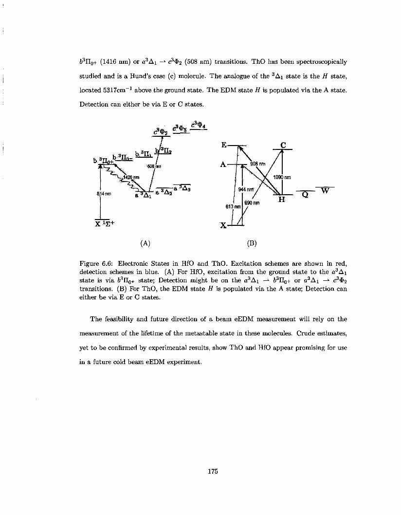
63n0+ (1416 nm) or a3Aj —* c34>2 (508 nm) transitions. ThO has been spectroscopically
studied and is a Hund's case (c) molecule. The analogue of the 3Ai state is the H state,
located 5317cm-1 above the ground state. The EDM state H is populated via the A state.
Detection can either be via E or C states.
e»% < * » ^
X *£+•
(A) (B)
Figure 6.6: Electronic States in HfO and ThO. Excitation schemes are shown in red, detection schemes in blue. (A) For HfO, excitation from the ground state to the a3Ai state is via 63I10+ state; Detection might be on the a3Ai —»• fe3n0+ or a3Ai —*• c34>2 transitions. (B) For ThO, the EDM state H is populated via the A state; Detection can either be via E or C states.
The feasibility and future direction of a beam eEDM measurement will rely on the
measurement of the lifetime of the metastable state in these molecules. Crude estimates,
yet to be confirmed by experimental results, show ThO and HfO appear promising for use
in a future cold beam eEDM experiment.
175
Bibliography
[1] J. H. Christenson, J. W. Cronin, V. L. Fitch, and R. Turlay. Evidence for the 2n
decay of the Kg meson. Physical Review Letters, 13(4): 138-140, Jul 1964.
[2] B. Aubert, D. Boutigny, J.-M. Gaillard, A. Hicheur, Y. Karyotakis, J. P. Lees,
P. Robbe, V. Tisserand, A. Palano, G. P. Chen, J. C. Chen, N. D. Qi, G. Rong,
P. Wang, Y. S. Zhu, G. Eigen, P. L. Reinertsen, B. Stugu, B. Abbott, G. S. Abrams,
A. W. Borgland, A. B. Breon, D. N. Brown, J. Button-Shafer, R. N. Cahn, A. R.
Clark, and M. S. Gill. Observation of CP violation in the B° meson system. Physical
Review Letters, 87(9):091801, Aug 2001.
[3] K. Abe, K. Abe, R. Abe, I. Adachi, Byoung Sup Ahn, H. Aihara, M. Akatsu, G. Al-
imonti, K. Asai, M. Asai, Y. Asano, T. Aso, V. Aulchenko, T. Aushev, A. M. Bakich,
E. Banas, S. Behari, P. K. Behera, D. Beiline, A. Bondar, A. Bozek, T. E. Browder,
B. C. K. Casey, P. Chang, Y. Chao, K.-F. Chen, and B. G. Cheon. Observation of large
CP violation in the neutral B meson system. Physical Review Letters, 87(9):091802,
Aug 2001.
[4] M. E. Pospelov and I. B. Khriplovich. Electric-dipole moment of the W-boson and the
electron in the Kobayashi-Maskawa Model. Soviet Journal of Nuclear Physics- USSR,
53:638-640, 1991.
[5] A. D. Sakharov. Violation of cp invariance, c asymmetry, and baryon asymmetry of
the universe. Soviet Journal of Experimental and Theoretical Physics Letters, 5:24,
176
jan 1967.
[6] B. C. Regan, E. D. Commins, C. J. Schmidt, and D. DeMille. New limit on the
electron electric dipole moment. Physical Review Letters, 88:071805, 2002.
[7] D. F. Nelson, A. A. Schupp, R. W. Pidd, and H. R. Crane. Search for an electric
dipole moment of the electron. Physical Review Letters, 2(12):492-495, Jun 1959.
[8] S. RosendorfF. Upper limit for the intrinsic electric dipole moment of the proton and
the neutrino. Nuovo Cimento, 27:251, 1960.
[9] J. Bailey, K. Borer, F. Combleyg, H. Drummil, , W. Flegel, P.M. Hattersley, F.J.M.
Farley, J.H. Field, F. Krienen, F. Langell, E. Picasso, and W. von Rudenil. New limits
on the electric dipole moment of positive and negative muons. Journal of Physics G,
4:345-352, 1978.
[10] L. Pondrom, R. Handler, M. Sheaff, P.T. Cox, J. Dworkin, O.E. Overseth, T. Devlin,
L. Schachinger, and K. Heller. New limit on the electric dipole moment of the A0
hyperon. Physical Review D, 23:814-816, 1981.
[11] R. Escribano and E. Massd. New bounds on the magnetic and electric moments of
the T lepton. Physical Review D, 301:419-422, 1993.
[12] E. M. Purcell and N. F. Ramsey. On the possibility of electric dipole moments for
elementary particles and nuclei. Physical Review, 78(6):807, Jun 1950.
[13] C. A. Baker, D. D. Doyle, P. Geltenbort, K. Green, M. G. D. van der Grinten, P. G.
Harris, P. Iaydjiev, S. N. Ivanov, D. J. R. May, J. M. Pendlebury, J. D. Richardson,
D. Shiers, and K. F. Smith. Improved experimental limit on the electric dipole moment
of the neutron. Physical Review Letters, 97(13): 131801, Sep 2006.
[14] T. M. Ito and the n EDM Collaboration. Plans for a neutron EDM experiment at
SNS. Journal of Physics Conference Series, 69:2037, May 2007.
177
[15] S. K. Lamoreaux. Relativity - testing times in space. Nature, 416:803-804, 2002.
[16] B. J. Heidenreich, O. T. Elliott, N. D. Charney, K. A. Virgien, A. W. Bridges, M. A.
McKeon, S. K. Peck, D. Krause, J. E. Gordon, L. R. Hunter, and S. K. Lamoreaux.
Limit on the electron electric dipole moment in gadolinium-iron garnet. Physical
Review Letters, 95:253004, 2005.
[17] Edward A. Hinds and P. G. H. Sandars. Experiment to search for P- and T- violating
interactions in the hyperfine structure of thallium fluoride. Physical Review A, 21:480-
487, 1980.
[18] M. V. Romalis, W. C. Griffith, J. P. Jacobs, and E. N. Fortson. New limit on the
permanent electric dipole moment of Hg-199. Physical Review Letters, 86:2505-2508,
2001.
[19] Eugene D. Commins and David P. DeMille. Lepton dipole moments, chapter the
electric dipole moment of the electron, to be published, in 2008.
[20] D. DeMille, F. Bay, S. Bickman, D. Kawall, D. Krause, S. E. Maxwell, and L. R.
Hunter. Investigation of PbO as a system for measuring the electric dipole moment
of the electron. Physical Review A, 61:05250, 2000.
[21] A. Derevianko and M. G. Kozlov. Molecular CP-violating magnetic moment. Physical
Review A, 72:040101, 2005.
[22] L. I. Schiff. Measurability of nuclear electric dipole moments. Physical Review, 1:2194,
1963.
[23] P. G. H. Sandars. Electric dipole moment of an atom. Physics Letters, 14:194, 1965.
[24] Eugene D. Commins, J. David Jackson, and David P. DeMille. The electric dipole
moment of the electron: An intuitive explanation for the evasion of Schiff's theorem.
American Journal of Physics, 75(6):532-536, 2007.
178
[25] W. R. Johnson, D. S. Guo, M. Idrees, and J. Sapirstein. Weak-interaction effects in
heavy atomic systems II. Physical Review A, 34(2):1043-1057, Aug 1986.
[26] J. J. Hudson, B. E. Sauer, M. R. Tarbutt, and E. A. Hinds. Measurement of
the electron electric dipole moment using YbF molecules. Physical Review Letters,
89(2):023003, Jun 2002.
[27] M. G. Kozlov. Semiempirical calculations of P-odd and P,T-odd effects in diatomic
molecule-radicals. Zhurnal Eksperimentalnoi I Teoreticheskoi Fiziki, 89:1933-1940,
1985.
[28] M. G. Kozlov. Enhancement of the electric dipole moment of the electron in the YbF
molecule. Journal of Physics B-Atomic Molecular and Optical Physics, 30:L607-L612,
1997.
[29] N S Mosyagin, M G Kozlov, and A V Titov. Electric dipole moment of the electron
in the YbF molecule. Journal of Physics B: Atomic, Molecular and Optical Physics,
31(19):L763-L767, 1998.
[30] Y. Y. Dmitriev, Y. G. Khait, M. G. Kozlov, L. N. Labzovsky, A. O. Mitrushenkov,
A. V. Shtoff, and A. V. Titov. Calculation of the spin-rotational hamiltonian including
P-odd and P, T-odd weak interaction terms for HgF and PbF molecules. Physics
Letters A, 167:280-286, 1992.
[31] A. N. Petrov, A. V. Titov, T. A. Isaev, N. S. Mosyagin, and D. DeMille. Configuration-
interaction calculation of hyperfine and P,T-odd constants on 207PbO excited states
for electron electric-dipole-moment experiments. Physical Review A, 72:022505, 2005.
[32] T. A. Isaev, A. N. Petrov, N. S. Mosyagin, and A. V. Titov. In search of the electron
electric dipole moment: Relativistic correlation calculations of the P,T-violating effect
in the ground state of HI+. Physical Review Letters, 95(16):163004, 2005.
179
[33] E. R. Meyer, J. L. Bohn, and M. P. Deskevich. Candidate molecular ions for an
electron electric dipole moment experiment. Physical Review A, 73:062108, 2006.
[34] R. C. Oldenborg, C. R. Dickson, and R. N. Zare. A new electronic band system of
PbO. Journal of Molecular Spectroscopy, 58:283-300, 1975.
[35] M. G. Kozlov and D. DeMille. Enhancement of the electric dipole moment of the
electron in PbO. Physical Review Letters, 89:133001, 2002.
[36] W. H. Beattie, M. A. Revelli, and J. M. Brom. Radiative lifetime of PbO a(l). Journal
of Molecular Spectroscopy, 70:163-164, 1978.
[37] J. M. Brown, J. T. Hougen, K.-P. Huber, J. W. C. Johns, I. Kopp, H. Lefebvre-Brion,
A. J. Merer, D. A. Ramsay, J. Rostas, and R. N. Zare. The labeling of parity doublet
levels in linear molecules. Journal of Molecular Spectroscopy, 55:500-503, Mar 1975.
[38] F. Martin, R. Bacis, J. Verges, J. Bachar, and S. Rosenwaks. High-resolution Fourier-
transform spectroscopy of the PbO molecule from investigation of the 0[2]([l]A[g])-
Pb reaction. Spectrochimica Acta Part a-Molecular and Biomolecular Spectroscopy,
44:889-897, 1988.
[39] D. Kawall, F. Bay, S. Bickman, Y. Jiang, and D. DeMille. Precision Zeeman-Stark
spectroscopy of the metastable a(l) [3S+] state of PbO. Physical Review Letters,
92:133007, 2004.
[40] J. T. Hougen. The calculation of rotational energy levels and rotational line intensities
in diatomic. NBS Monograph 115, 1970.
[41] L. R. Hunter, S. E. Maxwell, K. A. Ulmer, N. D. Charney, S. K. Peck, D. Krause,
S. Ter-Avetisyan, and D. DeMille. Detailed spectroscopy of the a(l) [3S+] state of
PbO. Physical Review A, 65:030501, 2002.
[42] S. Haroche. High-Resolution Laser Spectroscopy, chapter: Quantum Beats and Time-
Resolved Fluorescence Spectroscopy. Springer-Verlag, 1976.
180
[43] G. J. Gemmen and N. Rouze. Analysis of idealized Zeeman quantum beat experiments
in the advanced laboratory. American Journal of Physics, 64:147-150, 1996.
[44] Weng W. Chow, Marian O. Scully, and John O. Stoner. Quantum-beat phenomena
described by quantum electrodynamics and neoclassical theory. Physical Review A,
11 (4): 1380-1388, Apr 1975.
[45] Predrik Bay. Construction of an Apparatus and Preliminary Measurements for a
Search for the Electric Dipole Moment of the Electron using Lead Monoxide. PhD
thesis, Yale University, 2003.
[46] William H. Press, Saul A. Teukolsky, William T. Vetterling, and Brian P. Flannery.
Numerical recipes in C++ : the art of scientific computing, Second Edition. Cambridge
Univeristy Press, 2002.
[47] L. Duong and Muon g-2 Collaboration. Muon g-2 measurement: The Ratio Fit
method. Bulletin of the American Physical Society, 46(2):C10.003, April 2001.
[48] Jonathan M. Paley. Measurement of the anomalous magnetic moment of the negative
muon to 0.7 parts per million. PhD thesis, Boston University, 2004.
[49] E. D. Commins, S. B. Ross, D. DeMille, and B. C. Regan. Improved experimental
limit on the electric-dipole moment of the electron. Physical Review A, 50:2960-2977,
1994.
[50] Eugene D. Commins. Berry's geometric phase and motional fields. American Journal
of Physics, 59(12):1077-1080, 1991.
[51] J. M. Pendlebury, W. Heil, Y. Sobolev, P. G. Harris, J. D. Richardson, R. J. Baskin,
D. D. Doyle, P. Geltenbort, K. Green, M. G. D. van der Grinten, P. S. Iaydjiev, S. N.
Ivanov, D. J. R. May, and K. F. Smith. Geometric-phase-induced false electric dipole
moment signals for particles in traps. Physical Review A, 70:032102, 2004.
181
[52] S. K. Lamoreaux and R. Golub. Detailed discussion of a linear electric field frequency
shift induced in confined gases by a magnetic field gradient: Implications for neutron
electric-dipole-moment experiments. Physical Review A, 71(3):032104, 2005.
[53] D. S. Weiss, F. Fang, and J. Chen. Measuring the electric dipole moment of Cs and
Rb in an optical lattice. APS Meeting Abstracts, page J1.008, Apr 2003.
[54] C. DeMicco and C. M. Aldao. On the net radiation method for heat transfer. European
Journal of Physics, 24:81-89, Jan 2003.
[55] C. V. Dodd and W. E. Deeds. Analytical solutions to eddy-current probe-coil prob
lems. Journal of Applied Physics, 39(6):2829-2838, 1968.
[56] T. S. E. Thomas. Screening effect of a circular disk. American Journal of Physics,
29:37-39, Jan 1961.
[57] Kent Davey and Larry Turner. The use of time space green's functions in the compu
tation of transient eddy current fields. Journal of Applied Physics, 64(11):6132-6137,
1988.
[58] W. M. Saslow. Maxwell's theory of eddy currents in thin conducting sheets, and
applications to electromagnetic shielding and maglev. American Journal of Physics,
60:693-711, Aug 1992.
[59] D. Schieber. Transient eddy currents in thin metal sheets. IEEE Transactions on
Magnetics, MAG-8(4):775, 1972.
[60] P. Horowitz and W. Hill. The Art of Electronics. Cambridge University Press, 2nd
ed., 1989.
[61] D. Shin and R. Magnusson. Diffraction by surface-relief gratings with conic cross-
sectional grating shapes. Journal of the Optical Society of America A, 6:1249-1253,
Sep 1989.
182
[62] Tasso R. M. Sales. Structured microlens arrays for beam shaping. Optical Engineering,
42(ll):3084-3085, 2003.
[63] W.T. Welford and R. Winston. The Optics of Nonimaging Concentrators. Academic
Press Inc, 1978.
[64] Sarah Bickman. Progress towards a Measurement of the Electric Dipole Moment of
the Electron using PbO*. PhD thesis, Yale University, 2007.
[65] Jr. J. M. Brom and W. H. Beattie. Laser excitation spectrum of PbO : Rotational
analysis of the a(l)-x(0+) system. Journal of Molecular Spectroscopy, 81:445, 1980.
[66] J. Bachar, R. Bacis, S. Churassy, F. Martin, S. Rosenwaks, G. Taieb, and J. Verges.
PbO spectroscopy and studies of the interaction of singlet molecular-oxygen with
lead atoms by laser-induced fluorescence and by high-resolution Fourier-transform
spectroscopy. Journal De Physique, 48:381-383, 1987.
[67] Clarence Zener. Non-adiabatic crossing of energy levels. Proc. R. Soc. A, 137:696,
1932.
[68] I. S. Gradshteyn and I. M. Ryzhik. Table of integrals, series and products. Academic
Press, 1994.
[69] N. V. Vitanov and B. M. Garraway. Landau-Zener model: Effects of finite coupling
duration. Physical Review A, 53(6):4288-4304, Jun 1996.
[70] S. Thomas, S. Guerin, and H. R. Jauslin. State-selective chirped adiabatic passage on
dynamically laser-aligned molecules. Physics Review A, 71(1):013402, 2005.
[71] Wolfgang Petrich, Michael H. Anderson, Jason R. Ensher, and Eric A. Cornell. Stable,
tightly confining magnetic trap for evaporative cooling of neutral atoms. Physical
Review Letters, 74(17) :3352-3355, Apr 1995.
[72] Misha Lukin. . private communication, 2007.
183
[73] David R. Lide and H.P.R. Prederikse. CRC Handbook of chemistry and physics. Chem
ical Rubber Publishing Company, 1995.
[74] J. Drowart, R. Colin, and G. Exsteen. Mass-spectrometric study of the vaporization
of lead monoxide*. Transactions of the Faraday Society, 61:1376-1383, 1965.
[75] R.H. Lamoreaux and D.L. Hildenbrand. High temperature vaporization behavior of
oxides II: Oxides of Be, Mg, Ca, Sr, Ba, B, Al, Ga, In, Tl, Si, Ge, Sn, Pb, Zn, Cd,
and Hg. Journal of Physical and Chemical Reference Data, 16(3):419-443, 1987.
[76] A. Popovic, A. Lesar, M. Gucek, and L. Bencze. Mass spectrometric investigation of
the evaporation properties of lead oxide. Rapid Communications in Mass Spectrome
try, 11:459-468, 1997.
[77] S.I. Lopatin, I.Ya. Mittova, F.S. Gerasimov, S.M. Shugurov, V.F. Kostryukov, and
S.M. Skorokhodova. Vaporization and thermodynamic properties of the PbO-V20s
system. Physiochemical Analysis of Inorganic Systems, 51(10):1646-1652, 2005.
[78] Richard G. Brewer and E. L. Hahn. Coherent raman beats. Physical Review A,
8(l):464-472, Jul 1973.
[79] Richard G. Brewer and E. L. Hahn. Coherent two-photon processes: Transient and
steady-state cases. Physical Review A, 11 (5): 1641-1649, May 1975.
[80] Derek F. Kimball Dmitry Budker and David P. DeMille. Atomic physics An Explo
ration Through Problems and Solutions. Oxford University Press, 2004.
[81] Amar Vutha. Molecules for a cold beam EDM experiment, private communication,
2007.
[82] A. N. Petrov, N. S. Mosyagin, T. A. Isaev, and A. V. Titov. Towards the electron
EDM search: Theoretical study of HfF+. ArXiv.physics/0611254, 2006.
184