Embed Size (px)
DESCRIPTION
Publications on advanced studies in theoretical and experimental physics, including related themes from mathematics.
Citation preview
2008, VOLUME 4
PROGRESS
IN PHYSICS
“All scientists shall have the right to present their scien-tific research results, in whole or in part, at relevant sci-entific conferences, and to publish the same in printedscientific journals, electronic archives, and any othermedia.” — Declaration of Academic Freedom, Article 8
ISSN 1555-5534
The Journal on Advanced Studies in Theoretical and Experimental Physics, including Related Themes from Mathematics
PROGRESS IN PHYSICSA quarterly issue scientific journal, registered with the Library of Congress (DC, USA). This journal is peer reviewed and included in the ab-stracting and indexing coverage of: Mathematical Reviews and MathSciNet (AMS, USA), DOAJ of Lund University (Sweden), Zentralblatt MATH(Germany), Scientific Commons of the University of St. Gallen (Switzerland), Open-J-Gate (India), Referativnyi Zhurnal VINITI (Russia), etc.
To order printed issues of this journal, con-tact the Editors. Electronic version of thisjournal can be downloaded free of charge:http://www.ptep-online.comhttp://www.geocities.com/ptep online
Editorial Board
Dmitri Rabounski (Editor-in-Chief)[email protected] [email protected] [email protected] J. [email protected]
Postal address
Chair of the Departmentof Mathematics and Science,University of New Mexico,200 College Road,Gallup, NM 87301, USA
Copyright c© Progress in Physics, 2007
All rights reserved. The authors of the ar-ticles do hereby grant Progress in Physicsnon-exclusive, worldwide, royalty-free li-cense to publish and distribute the articles inaccordance with the Budapest Open Initia-tive: this means that electronic copying, dis-tribution and printing of both full-size ver-sion of the journal and the individual paperspublished therein for non-commercial, aca-demic or individual use can be made by anyuser without permission or charge. The au-thors of the articles published in Progress inPhysics retain their rights to use this journalas a whole or any part of it in any other pub-lications and in any way they see fit. Anypart of Progress in Physics howsoever usedin other publications must include an appro-priate citation of this journal.
This journal is powered by LATEX
A variety of books can be downloaded freefrom the Digital Library of Science:http://www.gallup.unm.edu/�smarandache
ISSN: 1555-5534 (print)ISSN: 1555-5615 (online)
Standard Address Number: 297-5092Printed in the United States of America
OCTOBER 2008 VOLUME 4
CONTENTS
P. Wagener A Unified Theory of Interaction: Gravitation and Electrodynamics . . . . . . . . . . 3
E. Goldfain and F. Smarandache On Emergent Physics, “Unparticles” and Exotic“Unmatter” States . . . . . . . . . . . . . . . . . . . . . . . . . . . . . . . . . . . . . . . . . . . . . . . . . . . . . . . . . . . 10
M. Harney and I. I. Haranas The Dark Energy Problem . . . . . . . . . . . . . . . . . . . . . . . . . . . . . 16
R. T. Cahill Unravelling Lorentz Covariance and the Spacetime Formalism . . . . . . . . . . . . . 19
Xiao-Song Wang Derivation of the Newton’s Law of Gravitation Based on a FluidMechanical Singularity Model of Particles . . . . . . . . . . . . . . . . . . . . . . . . . . . . . . . . . . . . . 25
G. I. Garas’ko A Method of Successive Approximations in the Framework of the Geom-etrized Lagrange Formalism . . . . . . . . . . . . . . . . . . . . . . . . . . . . . . . . . . . . . . . . . . . . . . . . . . 31
Huy Khanh Hoang Instant Interpretation of Quantum Mechanics . . . . . . . . . . . . . . . . . . . . . 37
I. A. Abdallah, A. F. Hassan, and I. M. Tayel Thermoelastic Property of a Semi-InfiniteMedium Induced by a Homogeneously Illuminating Laser Radiation . . . . . . . . . . . . . . 44
S. M. Diab and S. A. Eid Nature of the Excited States of the Even-Even 98-108Ru Iso-topes . . . . . . . . . . . . . . . . . . . . . . . . . . . . . . . . . . . . . . . . . . . . . . . . . . . . . . . . . . . . . . . . . . . . . . . 51
Information for Authors and Subscribers
Progress in Physics has been created for publications on advanced studies intheoretical and experimental physics, including related themes from mathe-matics and astronomy. All submitted papers should be professional, in goodEnglish, containing a brief review of a problem and obtained results.
All submissions should be designed in LATEX format using Progress inPhysics template. This template can be downloaded from Progress in Physicshome page http://www.ptep-online.com. Abstract and the necessary informa-tion about author(s) should be included into the papers. To submit a paper,mail the file(s) to the Editor-in-Chief.
All submitted papers should be as brief as possible. We usually acceptbrief papers, no larger than 8–10 typeset journal pages. Short articles arepreferable. Large papers can be considered in exceptional cases to the sec-tion Special Reports intended for such publications in the journal. Lettersrelated to the publications in the journal or to the events among the sciencecommunity can be applied to the section Letters to Progress in Physics.
All that has been accepted for the online issue of Progress in Physics isprinted in the paper version of the journal. To order printed issues, contactthe Editors.
This journal is non-commercial, academic edition. It is printed from pri-vate donations. (Look for the current author fee in the online version of thejournal.)
October, 2008 PROGRESS IN PHYSICS Volume 4
A Unified Theory of Interaction: Gravitation and Electrodynamics
Pieter Wagener
Department of Physics, Nelson Mandela Metropolitan University, Port Elizabeth, South AfricaE-mail: [email protected]
A theory is proposed from which the basic equations of gravitation and electromag-netism are derived from a single Lagrangian. The total energy of an atom can be ex-pressed in a power series of the fine structure constant, �. Specific selections of theseterms yield the relativistic correction to the Bohr values of the hydrogen spectrum andthe Sommerfeld-Dirac equation for the fine structure spectrum of the hydrogen atom.Expressions for the classical electron radius and some of the Large Number Coinci-dences are derived. A Lorentz-type force equation is derived for both gravitation andelectrodynamics. Electron spin is shown to be an effect of fourth order in �.
1 Introduction
In a previous article [2] in this journal we presented a clas-sical Lagrangian characterizing the dynamics of gravitationalinteraction,
L = �m0(c2 + v2) expR=r; (1)
where we denote:m0 = gravitational rest mass of a test body mov-
ing at velocity v in the vicinity of a mas-sive, central body of mass M ,
= 1=p
1� v2=c2,R = 2GM=c2 is the Schwarzschild radius of the
central body.The following conservation equations follow:
E = mc2eR=r = total energy = constant ; (2)L = eR=rM = constant; (3)Lz = MzeR=r = eR=rm0r2 sin2� _� (4)
= z component of L = constant;
where m = m0= 2 and
M = (r�m0v) (5)
is the total angular momentum of the test body.It was shown that the tests for perihelion precession and
the bending of light by a massive body are satisfied by theequations of motion derived from the conservation equations.
The kinematics of the system is determined by assumingthe local and instantaneous validity of special relativity (SR).This leads to an expression for gravitational redshift:
� = �0 e�R=2r; (�0 = constant) , (6)
which agrees with observation.Electrodynamics is described by the theory of special rel-
ativity. If the motion of a particle is dynamically determined
by the above Lagrangian, then a description of the kinematicsof its motion in terms of special relativity should yield equa-tions of motion analogous to those of electrodynamics. This,in principle, should allow the simultaneous manifestation ofgravitation and electrodynamics in one model of interaction.
We follow this approach and show, amongst others, thatelectrical charge arises from a mathematical necessity forbound motion. Other expressions, such as the classical elec-tron radius and expressions of the Large Number Hypothesisfollow.
The total energy for the hydrogen atom can be expressedin terms of a power series of the fine structure constant, �.Summing the first four terms yields the Sommerfeld-Diracexpression for the total energy. For higher order terms thefinite radius of the nucleus must be taken into account. Thisintroduces a factor analogous to “electron spin”.
Details of all calculations are given in the PhD thesis ofthe author [1].
2 Gravitation and Special Relativity
Einstein’s title of his 1905 paper, Zur Elektrodynamik be-wegter Korper indicates that electrodynamics and SR are in-terrelated, with SR giving an explanation for certain proper-ties of electrodynamics. Red-shift is such a property, combin-ing both gravitation and electromagnetism in a single formu-lation, and should provide us with a dynamical link betweenthese two phenomena. To do this, we substitute the photo-electric effect,
h� = ~mc2; (7)
where ~m = ~m0 and ~m0 is the electromagnetic rest mass ofa particle, into (6). This gives
E = ~mc2eR=2r = ~m0c2eR=2rp
1� v2=c2= ~EeR=2r
= ~m0c2 + ~m0v2=2 + ~m0Rc2=2r++ ~m0Rv2=4r + : : :
9>>>>=>>>>; ; (8)
Pieter Wagener. A Unified Theory of Gravitation and Electrodynamics 3
Volume 4 PROGRESS IN PHYSICS October, 2008
where E is another constant of energy and ~E = ~mc2 is thetotal energy of the theory of special relativity.
Let us compare this expansion with the expansion of (2)for the gravitational energy,
m0c2 � E2
=m0v2
2� GMm0
r+m0v2R
2r�
� m0c2R2
4r2 +m0v2R2
4r2 + : : :(9)
The negative sign of the second right hand term in (9)ensures attractive, or bound, motion under gravitation. In or-der for the motion determined by (8) to be bounded, the thirdright hand term must similarly be negative and inversely pro-portional to r. To ensure this we let
~m0c2 = �e2=re; (10)
where e2 is an arbitrary constant and
re = R=2: (11)
Eq.(8) can then be rewritten as
E = ~mc2ere=r: (12)
As we shall see for the hydrogen atom, e represents theelectron charge, re represents the classical electron radius and(11) yields some of the numbers of Dirac’s Large NumberHypothesis.
The choice of a positive sign in (10) gives repulsive mo-tion. Such a freedom of choice is not possible for the gravita-tional energy of (9).
2.1 Hamiltonian formulation
Confirmation of the above conclusions can be found by exam-ining the predictions for the hydrogen spectrum. We followa classical approach based on the principles of action vari-ables [3].
Using the identity 2 = 1 + 2v2=c2 to separate the ki-netic and potential energies in (8), a corresponding Lagran-gian can be found:
L = � ~m0c2p
1� v2=c2 exp(re=r): (13)
We obtain the conjugate momenta:
pr = ~m _r exp(re=r) ; (14)
p� = ~mr2 _� exp(re=r) ; (15)
p� = ~mr2 sin2� _� exp(re=r) : (16)
The associated Hamiltonian can be derived from the for-mula H =
P_qipi � L as follows
H =�
~m20c
4 exp(re=r) +
+ c2(p2r + p2
�=r2 + p2
�=r2 sin2�)
�1=2: (17)
From the canonical equations
_pi =@H@qi
; (18)
we find the following conservation equations:
L2 �M2 exp(2re=r) = p2� + p2
�= sin2� ; (19)
Lz �Mz exp(re=r) = p� ; (20)
where L2 and Lz are constants and
M = (r� ~mv); (21)
is the total angular momentum of the orbiting particle.It should be noted that (12), (19), (20) and (21) have re-
spectively the same forms as for the gravitational equations(2), (3), (4), (5), but withm = m0= 2 replaced by ~m = ~m0and R by re = R=2.
3 The hydrogen spectrum
In order to determine an expression for the energy levels ofthe H-atom, two different approaches can be followed: (i)Analogously to the Wilson-Sommerfeld model, one can ap-ply the procedures of action angle variables, or (ii) pertur-bation theory, where the contribution of each energy term isevaluated separately.
To generalize our discussion we shall, where appropriate,use a general potential � = Rc2=2r = rec2=r:
3.1 Method of action angle variables
The theory of action angle variables originated in the de-scription of periodic motion in planetary mechanics [4, Ch.9].From that theory Wilson and Sommerfeld postulated thequantum condition:
For any physical system in which the coordinatesare periodic functions of time, there existsa quantum condition for each coordinate. Thesequantum conditions are
Ji =Ipidqi = nih ; (22)
where qi is one of the coordinates, pi is the mo-mentum associated with that coordinate, ni is aquantum number which takes on integral values,and the integral is taken over one period of thecoordinate qi.
Applying these quantization rules to the conjugate mo-menta of (14), (15) and (16) gives [3]
Lz = Mz exp(re=r) = n� ~ ; (23)
L = M exp(re=r) = (n� + n�) ~ = k~ ; (24)H �E2=c2 � ~m2
0c2 exp(re=r)� k2~2=r2� 12 dr = nrh ; (25)
4 Pieter Wagener. A Unified Theory of Gravitation and Electrodynamics
October, 2008 PROGRESS IN PHYSICS Volume 4
where n�, n�, k and nr have the values 0, 1, 2, . . .To determine the atomic spectrum we need to evaluate the
integral of (25). Because of the finite radius of the nucleuswe choose an arbitrary effective nuclear radius of gre. Thepotential term in the exponentials is then written as
exp�
2�c2
�= exp
�2re
r � gre�; (26)
so that
exp(2�=c2) =
= 1 + 2rer
+ 2r2er2 (g + 1) + 3
r3er3 g (g + 1) + : : : (27)
For convenience we also define a parameter f such that
f = 2(g + 1) : (28)
We shall subsequently see that the value of g, or f , isrelated to the concept of electron spin.
Approximating (27) to second order in re=r, substitutingthis approximation in (25) and integrating gives
E2m = 1� �2h
n� k +pk2 + f�2
i2 ; (29)
where Em = E= ~m0c2, n = nr +k and � = e2=~c is the finestructure constant. This expression is simplified by expandingto fourth order in �:
Em � 1� �2
2n2
�1 +
�2
n
�1
4n� fk
��: (30)
The corresponding Sommerfeld/Dirac expressions are re-spectively
E2m =
1 +
�2�n� k +
pk2 � �2
�2!�1
(31)
and
Em � 1� �2
2n2
�1 +
�2
n
�1k� 3
4n
��; (32)
where k = j+ 12 for the Dirac expression, and j = 1
2 ;32 ;
52 ; : : :
: : : (n�1)2 .
The difference between the energy given by our modelEW , as given by (30), and that of the Sommerfeld-Diracmodel, ED, as given by (32), is
(ED � EW )= ~m0c2 =�4
2n3
�1k
(f + 1)� 1n
�: (33)
We shall show below that this difference corresponds tothe energy associated with the “spin-orbit” interaction of ourmodel.
4 Perturbation method
We use this method as applied by Born and others [3, Ch. 4].To apply the perturbation method we need to express the
energy ~E in terms of the momentum:
E = (p2c2 + ~m20c
4)1=2 exp(�=c2) ; (34)
where p = ~mv. Again, taking the finite radius of the nucleusinto account, we choose for the potential,
exp(�=c2) = exp�re=(r � gre)� ; (35)
so that the potential term can be written as
exp(�=c2) = 1 +rer
+wr2er2 +
�w2 � 1
4
�r3er3 + : : : ; (36)
wherew = (g + 1=2) = (f � 1)=2 : (37)
With this form for the potential, and using ~m0c2re =�e2,(34) can be expanded as
E = ~m0c2| {z }E0
+p2
2 ~m0� e2
r| {z }E1
� p4
8 ~m30c2| {z }E2
+p2re2 ~m0r| {z }E3
+
+ wr2e ~m0c2
r2| {z }E4
+wp2r2
e2 ~m0r2| {z }E5
� p4re8 ~m3
0c2r| {z }E6
+
+ ~m0c2�w2 � 1
4
�r3er3| {z }
E7
+ : : : (38)
Applying the unperturbed Bohr theory to each bracedterm, we find the following quantized expressions:
4.1 E0: rest mass energy
The first term on the right is the rest mass energy, which wedenote by E0:
E0 = ~m0c2: (39)
4.2 E1: Bohr energy
The next two terms represent the unperturbed Coulomb en-ergy of the hydrogen atom, which we indicate by E1:
E1 = p2=2 ~m0 � e2=r : (40)
According to the method of the Bohr theory,
E1 = �Re=n2; n = 1; 2; : : : (41)
where
Re =Ryhc = e2=2a0 = �2 ~m0c2=2a0 =Bohr radius = ~2= ~m0e2
Ry =Rydberg constant = 2�2e4 ~m0=ch3 = �=4�a0
9>=>; : (42)
Pieter Wagener. A Unified Theory of Gravitation and Electrodynamics 5
Volume 4 PROGRESS IN PHYSICS October, 2008
4.3 E2: relativistic correction
The third term is denoted by E2. It can be shown that [1]
E2 = � p4=8 ~m30c
2; (43)
= � �2Ren3
�1k� 3
4n
�: (44)
This is the “relativistic correction” of the Bohr-Sommer-feld model [3, §33]. This energy term is similar to that con-tained in the Dirac expression of (32). The sum of E0, E1and E2 gives an expression identical to that of Sommerfeldand similar to that of Dirac.
It is well-known that Sommerfeld’s result was fortuitousas the effect of spin-orbit coupling was ignored in his model.This effect is incorporated in the Dirac model. In our modelwe shall see below that E3 is an orbit-interaction term andthat E4 is related to ‘electron spin’. These two terms, missingin the Sommerfeld model, can now be added toE0 +E1 +E2of the Sommerfeld energy expression.
4.4 E3: orbital magnetic energy
We denote the fourth term by E3:
E3 = p2re=2 ~m0r : (45)
Applying the unperturbed Bohr theory, we find from (40):
E3 = (E1 + e2=r)re=r
= re(E1=r + e2=r2) : (46)
Using (41) and the average values [3, p144],
1=r = 1=n2a0 ; (47)
1=r2 = 1=a20n
3k ; k = 1; 2; : : : n (48)
as well asre=a0 = a2; (49)
we get
E3 =�2Ren3
�2k� 1n
�=�4 ~m0c2
2n3
�2k� 1n
�: (50)
The physical interpretation of E3 is that it is the energydue to the magnetic interaction of an electron moving in orbitabout a proton. This can be seen as follows.
Substituting p= ~mv and re =� e2= ~m0c2 into (45) gives
E3 = � e2v2
2rc2
�~m~m0
�2� � e2v2
2rc2in the non-relativistic limit: (51)
It corresponds to the classical form of the magnetic en-ergy due to orbital motion, as given by (70) below:
4.5 E4: “electron spin”
E4 = wr2e ~m0c2=r2;
= we4= ~m0c2r2:(52)
Applying (48) gives
E4 =w2�2Ren3k
= w�4 ~m0c21n3k
: (53)
We consider the significance of the factor w. We note thatthe potential energy expression (36) can be truncated after thequadratic term in re=r by letting w2� 1
4 = 0. As such, trun-cation can be considered as the limit to the resolution of theapparatus used for spectral observation. With this condition,we find that
w = � 12
(54)
gives the spectrum due to all interactions up to second degreein r=re. Therefore, from (42) and (53):
E4 = �12e8 ~m0
~4c21n3k
: (55)
The above expression for E4 corresponds to the quantummechanical result for the energy due to electron spin. Exceptfor the quantum numbers, Eisberg and Resnick [6, Example8–3] find a similar result for the energy due to spin-orbit in-teraction.
The equivalence of (55) to the result of Eisberg and Res-nick also confirms the implicit value gs = 2 in E4.
In this study E4 corresponds to the energy due to quan-tum mechanical spin only. Combining E3 and E4 gives thecorresponding total spin-orbit energy.
For k = 1 the expression for E4 is equal to the Darwinterm of the Dirac theory. In the Dirac theory the Darwin termhas to be introduced separately for ` = 0 states, whereas inour model E4 already provides for ` = 0 through the degen-eracy (` = 0; 1) associated with the k = 1 level.
In summary, ‘electron spin’ represents a second ordercontribution r2
e=r2 to the total energy of the atom.The above reasoning also applies to higher orders of ap-
proximation. Expanding (35) to fourth degree in re=r gives:
exp(�=c2) = 1 +rer
+r2er2w +
r3er3 (w2 � 1
2) +
+r4er4
�w2 � 1
4
�w + : : :
(56)
The coefficient of r4e=r4 is zero if (w2 � 1
4 )w = 0, or
w =12; �1
2; 0: (57)
A next higher resolution to r3e=r3 therefore introduces an
additional value of w = 0, giving a triplet symmetrical aboutthis value.
For a comprehensive survey of the conceptual develop-ments surrounding electron spin we refer to the text by To-monaga [7].
6 Pieter Wagener. A Unified Theory of Gravitation and Electrodynamics
October, 2008 PROGRESS IN PHYSICS Volume 4
4.6 E5: radiative reaction
E5 = wp2r2
e2 ~m0r2 (58)
= � 12�4Re
�1n5k� 2n3k3
�: (59)
Substituting p = ~mv in (58) gives
E5 = � 12
v2e4
2 ~m0c4r2
�~m~m0
�2: (60)
In the non-relativistic limit, ~m � ~m0, the above termcorresponds to the last RHS term of (69), i.e. the classicalenergy resulting from radiative reaction. Its value is too small(� 10�8 eV) to affect the values of the fine-spectrum.
4.7 Summary
E0 = m0c2 : rest mass energy;
E1 = �Ren2 : Bohr energy;
E2 = ��2Ren3
�1k� 3
4n
�: relativistic correction;
E3 =�2Ren3
�2k� 1n
�: orbital magnetic energy;
E4 = w2�2Ren3k
: electron spin energy;
E5 = w�4Re�
1n5k� 2n3k3
�: Radiative reaction;
where w = � 12 .
The sum of the energy termsPEi = E0 + E1 + E2 +
E3 + E4 + E5 is:XEi= ~m0c2 = 1� �2
2n2
�1� �2
n
�fk� 1
4n
��; (61)
which, as expected, is the same as (30).Each term in (38) can be related to a standard electro-
dynamic effect. It is significant that although (38) does notexplicitly contain any vector quantities, such as the vector po-tential A, this potential is implicit, as shown in the discussionof E3 and the comparison with (69).
An explanation for the difference (33) between the spec-trum of the proposed model and that of Dirac-Sommerfeldcan be seen as follows:
Consider the sum
E3 + E4 =�2Ren3
�2k
(w + 1)� 1n
�(62)
or, since w = (f � 1)=2,
E3 + E4 =�2Ren3
�1k
(f + 1)� 1n
�: (63)
The above equation corresponds to (33), the differencebetween the Sommerfeld-Dirac expression and that of ourmodel. The expression (30) therefore already incorporatesthe spin-orbit interaction.
The energy E3 + E4 therefore represents a perturbationto the Sommerfeld-Dirac values. The only candidate for thisperturbation is the Lamb-shift. For the (n; k) = (2,1) level andforw=� 0.5 the value ofE3+E4 is 4.52 831 78 e�5 ev. TheLamb-shift for this level is 4.37 380 19 e�6 eV, which is anorder 10 smaller. It would be overly ambitious to find the ob-served Lamb-shift from the present simple model. At this de-gree of spectral resolution one would have to look at a modifi-cation of the effective nuclear radius to r� a1re� a2r2
e � : : :
4.8 Comparison with classical electromagnetic energy
In order to compare the results of this study with those of con-ventional electromagnetic theory, we give a brief summary ofthe energy relations of classical electrodynamic theory.
The Hamiltonian describing the interaction of an electronwith fields H and E is given by [8, p. 124]
Hclassical = e� +�p� e
cA�2=2 ~m; (64)
where � and A are respectively the electrostatic and vectorpotentials of the system.
It is important to note that A and � do not merely repre-sent the external fields in which the particle moves, but alsothe particle’s own fields. This implies that the force of radia-tive reaction is automatically included.
The corresponding classical Lagrangian is
Lclassical =p2
2 ~m� e� +
ecA � v: (65)
For an electron moving under the influence of a magneticfield,
H = e (v � r)=cr3; (66)
a vector potential A can be found as
A =12
(H� r) = ev=2cr : (67)
Substituting this expression for A and using p = ~mv,yields �
p� ecA�2
= p2 � e2v2 ~mc2r
+e4v2
4c4r2 : (68)
Since the Hamiltonian of (64) does not contain t explic-itly, we may equate it to the total energy. Consequently, sub-stituting (68), and e� =� e2=r, in (64) gives the classical
Pieter Wagener. A Unified Theory of Gravitation and Electrodynamics 7
Volume 4 PROGRESS IN PHYSICS October, 2008
energy
Eclassical = �e2
r+
p2
2 ~m� e2v2
2c2r+
e4v2
8 ~mc4r2 : (69)
The third RHS term is the magnetic energy due to theorbital motion of the electron:
Eorbital = µ` �H = �g` e2v2
2rc2; (70)
where µ` = magnetic moment, g` = Lande g factor = 1, andM and H are parallel to one another. This energy correspondsto that of E3 above.
The fourth RHS term of (69) represents radiative reaction,which corresponds to our E5 as given by (60).
The standard relativistic Hamiltonian is given by:
Hrelativistic =�(p� qA=c)2c2 + ~m2
0c4� 1
2 + q� : (71)
The Hamiltonians of (64) and (71) must be compared toours of (17).
It is well-known that the Bohr model for the atom failsbecause of radiative reaction; in our model this loss is com-pensated for by the additional and associated potential term,E4, This term can also be interpreted as a modification ofCoulomb’s law. It is significant that this energy term can alsobe interpreted as arising from electron spin.
It is also significant that the Sommerfeld relativistic cor-rection term, E2, does not appear in either (69) or (71).
We can consider the electromagnetic energy arising fromthe Hamiltonians of (64) and (71) as approximations to thatof our Hamiltonian of (17).
We also note that the energy derived from the Hamilto-nian of (64), which is normally derived from a Lagrangiancontaining the vector potential A, appears as an approxima-tion to our model, which does not explicitly contain a vectorpotential. A vector potential arises in our theory because ofthe variation of mass according to (12).
5 The large number coincidences
Dirac postulated that the large dimensionless ratios (� 1040)of certain universal constants underlie a fundamental relation-ship between them. A theoretical explanation for these ratioshas not yet been found, but it became known as Dirac’s LargeNumber Hypothesis (LNH). [9] Some of these relations arederivable from (11).
Taking R as the Schwarzschild radius of the proton,Rp = 2GMp=c2, we rewrite (11) as
� e2
~m0c2=
GMp
c2
or � e2
GMp ~m0= 1: (72)
Defining the relationship between the gravitational massMp and the electromagnetic rest mass ~m0p of the proton as
Mp = ND ~m0p ; (73)
where ND is a dimensionless number, we can write (72) as
� e2
G ~M0p ~m0= ND ; (74)
which, if the absolute value is taken, is the basic relationshipof the LNH.
6 Lorentz force
The force equation for a particle, mass ~m and velocity vis found by applying the Euler-Lagrange equations to (13).This gives
_p = r~mrec2
r2 +~mrer3 v � (v � r) : (75)
Defining
E = rrec2
r2 ; (76)
H =rev � rr3 ; (77)
we can write (75) as
Electromagnetic _p = ~m�E + v �H
�: (78)
For v � c, ~mrec2 ! ~m0rec2 = e2 and then (75) ap-proaches the classical Lorentz form.
7 Unifying gravitation and electromagnetism
Equation (16) of reference [1] can be combined with (78) inone formulation:
_p = ~m�kE + v �H
�; (79)
where for
Gravitation : k = �1;Electromagnetism : k = 1:
The same equation gives either planetary or atomic mo-tion, where the vectors E and H are respectively given by
E = rGMr2 = r
rec2
r2 ; (80)
H =GM(v � r)
c2r3 =rev � rr3 : (81)
8 Pieter Wagener. A Unified Theory of Gravitation and Electrodynamics
October, 2008 PROGRESS IN PHYSICS Volume 4
8 Summary
Gravitation Electromagnetism
R = 2GM=c2 re = R=2m0 ~m0 = m0=N
L = �m0(c2 + v2)eR=r L = �( ~m0c2= )ere=r
E = mc2eR=r E = ~mc2ere=r
m = m0= 2 ~m = ~m0
L2 = M2e2R=r = constant L2 = M2e2re=r = constantLz = MzeR=r = constant Lz = Mzere=r = constant
M = (r�m0v) M = (r� ~m0v)_p = mE +m0v �H _p = ~m[E + v �H]
p = m0v p = ~mv
E = �rGM=r2 E = rrec2=r2
H = GM(v � r)=r3c2 H = re(v � r)=r3
9 Nuclear force
In a subsequent article we shall show that equations for thenuclear force, such as the Yukawa potential, can be derivedby considering the forms of both the energy equations (2) and(8) at r � R=2 = re:
Submitted on May 25, 2008Accepted on June 03, 2008
References
1. Wagener P.C. Principles of a theory of general interaction. PhDthesis, University of South Africa, 1987. An updated version isto be published as a book during 2008.
2. Wagener P.C. A classical model of gravitation. Progress inPhysics, 2008, v. 3, 21–23.
3. Born M. The mechanics of the atom. Frederick Ungar Publ.Co., New York, 1960.
4. Goldstein H. Classical Mechanics. Addison-Wesley, Reading,Mass., 1958.
5. Eisberg R.M. Fundamentals of modern physics. John Wiley,New York, 1961.
6. Eisberg R. and Resnick R. Quantum physics of atoms,molecules, solids, nuclei and particles. John Wiley, New York,1985.
7. Sin-Itiro Tomonaga. The story of spin. Univ Chicago Press,1997.
8. Grandy Jr. W.T. Introduction to electrodynamics and radiation.Academic Press, New York, 1970.
9. Harrison E.R. Physics Today, December 30, 1972.
Pieter Wagener. A Unified Theory of Gravitation and Electrodynamics 9

Volume 4 PROGRESS IN PHYSICS October, 2008
On Emergent Physics, “Unparticles” and Exotic “Unmatter” States
Ervin Goldfain� and Florentin Smarandachey� Photonics CoE, Welch Allyn Inc., Skaneateles Falls, NY 13153, USA
E-mail: [email protected] of Math & Sc. Depart., University of New Mexico, Gallup, NM 87301, USA
E-mail: [email protected]
Emergent physics refers to the formation and evolution of collective patterns in systemsthat are nonlinear and out-of-equilibrium. This type of large-scale behavior often de-velops as a result of simple interactions at the component level and involves a dynamicinterplay between order and randomness. On account of its universality, there are credi-ble hints that emergence may play a leading role in the Tera-ElectronVolt (TeV) sector ofparticle physics. Following this path, we examine the possibility of hypothetical high-energy states that have fractional number of quanta per state and consist of arbitrarymixtures of particles and antiparticles. These states are similar to “un-particles”, mass-less fields of non-integral scaling dimensions that were recently conjectured to emergein the TeV sector of particle physics. They are also linked to “unmatter”, exotic clustersof matter and antimatter introduced few years ago in the context of Neutrosophy.
1 Introduction
Quantum Field Theory (QFT) is a framework whose meth-ods and ideas have found numerous applications in variousdomains, from particle physics and condensed matter to cos-mology, statistical physics and critical phenomena [1, 2]. Assuccessful synthesis of Quantum Mechanics and Special Rel-ativity, QFT represents a collection of equilibrium field theo-ries and forms the foundation for the Standard Model (SM),a body of knowledge that describes the behavior of all knownparticles and their interactions, except gravity. Many brokensymmetries in QFT, such as violation of parity and CP in-variance, are linked to either the electroweak interaction orthe physics beyond SM [3–5]. This observation suggests thatunitary evolution postulated by QFT no longer holds near orabove the energy scale of electroweak interaction(� 300GeV) [6,7]. It also suggests that progress on the the-oretical front requires a framework that can properly handlenon-unitary evolution of phenomena beyond SM. We believethat fractional dynamics naturally fits this description. It op-erates with derivatives of non-integer order called fractal op-erators and is suitable for analyzing many complex processeswith long-range interactions [6–9]. Building on the currentunderstanding of fractal operators, we take the dimensionalparameter of the regularization program " = 4�d to representthe order of fractional differentiation in physical space-time(alternatively, " = 1 � d in one-dimensional space) [10, 11].It can be shown that " is related to the reciprocal of the cutoff
scale " � (�0/�), where �0 stands for a finite and arbitraryreference mass and � is the cutoff energy scale. Under thesecircumstances, " may be thought as an infinitesimal param-eter that can be continuously tuned and drives the departurefrom equilibrium. The approach to scale invariance demandsthat the choice of this parameter is completely arbitrary, as
long as " � 1. Full scale invariance and equilibrium fieldtheory are asymptotically recovered in the limit of physicalspace-time (d = 4) as "! 0 or �!1 [11, 12].
2 Definitions
We use below the Riemann-Liouville definition for the one-dimensional left and right fractal operators [13]. Consider forsimplicity a space-independent scalar field '(t). Taking thetime coordinate to be the representative variable, one writes
0D�L '(t) =
1�(1� �)
ddt
tZ0
(t� � )��'(� )d� ; (1)
0D�R '(t) =
1�(1� �)
(� ddt
)0Zt
(� � t)��'(� )d� : (2)
Here, fractional dimension 0 < � < 1 denotes the orderof fractional differentiation. In general, it can be shown that �is linearly dependent on the dimensionality of the space-timesupport [8]. By definition, � assumes a continuous spectrumof values on fractal supports [11].
3 Fractional dynamics and ‘unparticle’ physics
The classical Lagrangian for the free scalar field theory in3+1 dimensions reads [1–2, 14]
L = @�'@�'�m2'2; (3)
and yields the following expression for the field momentum
� =@L@(@'@t )
=@'@t
: (4)
10 Ervin Goldfain and Florentin Smarandache. On Emergent Physics, “Unparticles” and Exotic “Unmatter”
October, 2008 PROGRESS IN PHYSICS Volume 4
It is known that the standard technique of canonical quan-tization promotes a classical field theory to a quantum fieldtheory by converting the field and momentum variables intooperators. To gain full physical insight with minimal com-plications in formalism, we work below in 0+1 dimensions.Ignoring the left/right labels for the time being, we define thefield and momentum operators as
'! b' = ' ; (5)
� ! b�� = � i @�
@ j'j� � �iD�: (6)
Without the loss of generality, we set m = 1 in (3). TheHamiltonian becomes
H ! bH� = �12D2� +
12'2 =
12
(b�2� + '2) : (7)
By analogy with the standard treatment of harmonic oscil-lator in quantum mechanics, it is convenient to work with thedestruction and creation operators defined through [1–2, 14]
ba� :=1p2
[b'+ ib��] ; (8)
ba+� :=1p2
[b'� i b��] : (9)
Straightforward algebra shows that these operators satisfythe following commutation rules
[ba; ba] = [ba+�; ba+� ] = 0 ; (10)
[ba+�; ba� ] = i [ b'; b�� ] = �� b�(��1): (11)
The second relation of these leads tobH� = ba+� ba� +12�b�(��1): (12)
In the limit � = 1 we recover the quantum mechanics ofthe harmonic oscillator, namely
bH = ba+ba+12: (13)
It was shown in [6] that the fractional Hamiltonian (12)leads to a continuous spectrum of states having non-integernumbers of quanta per state. These unusual flavors of par-ticles and antiparticles emerging as fractional objects werenamed “complexons”. Similar conclusions have recently sur-faced in a number of papers where the possibility of a scale-invariant “hidden” sector of particle physics extending be-yond SM has been investigated. A direct consequence of thissetting is a continuous spectrum of massless fields havingnon-integral scaling dimensions called “un-particles”. Thereader is directed to [15–21] for an in-depth discussion of“un-particle” physics.
4 Mixing properties of fractal operators
Left and right fractal operators (L/R) are natural analogues ofchiral components associated with the structure of quantumfields [8, 9]. The goal of this section is to show that there is aninherent mixing of (L/R) operators induced by the fractionaldynamics, as described below. An equivalent representationof (1) is given by
0D�L '(t) =
1�(1��)
(� ddt
)0Zt
[�(��t)]��'(� ) d� ; (14)
or
0D�L '(t) =
(�1)���(1� �)
�� ddt
� 0Zt
(� � t)��'(� ) d� =
= (�1)�� 0D�R '(t) ; (15)
0D�R = (�1)� 0D�
L = exp(i��) 0D�L : (16)
Starting from (2) instead, we find
0D�L = (�1)� 0D�
R = exp(i��) 0D�R : (17)
Consider now the one-dimensional case d = 1, take� = " = 1�d and recall that continuous tuning of " does notimpact the physics as a consequence of scale invariance. Letus iterate (16) and (17) a finite number of times (n > 1) underthe assumption that n"� 1. It follows that the fractal opera-tor of any infinitesimal order may be only defined up to an ar-bitrary dimensional factor exp(i�n") � 1+(i�n") = 1�ie",that is,
0D"L;R '(t) � �0D0
L;R � ie"�'(t) (18)
ori0D"
L;R '(t) =�i 0D0
L;R + e"�'(t) ; (19)
wherelim"!0
D"L;R '(t) = '(t) : (20)
Relations (18–20) indicate that fractional dimension e" in-duces: (a) a new type of mixing between chiral componentsof the field and (b) an ambiguity in the very definition of thefield, fundamentally different from measurement uncertain-ties associated with Heisenberg principle. Both effects areirreversible (since fractional dynamics describes irreversibleprocesses) and of topological nature (being based on the con-cept of continuous dimension). They do not have a counter-part in conventional QFT.
5 Emergence of “unmatter” states
Using the operator language of QFT and taking into account(6), (18) can be presented asb�"'(t) = b�"'(t)� e" b'(t) : (21)
Ervin Goldfain and Florentin Smarandache. On Emergent Physics, “Unparticles” and Exotic “Unmatter” 11
Volume 4 PROGRESS IN PHYSICS October, 2008
Relation (21) shows that the fractional momentum op-erator b�" and the field operator b'(t) ='(t) are no longerindependent entities but linearly coupled through fractionaldimension e". From (11) it follows that the destruction andcreation operators are also coupled to each other. As a re-sult, particles and antiparticles can no longer exist as linearlyindependent objects. Because e" is continuous, they emergeas an infinite spectrum of mixed states. This surprising find-ing is counterintuitive as it does not have an equivalent inconventional QFT. Moreover, arbitrary mixtures of particlesand antiparticles may be regarded as a manifestation of “un-matter”, a concept launched in the context of NeutrosophicLogic [22–24].
6 Definition of unmatter
In short, unmatter is formed by matter and antimatter thatbind together [23, 24].
The building blocks (most elementary particles known to-day) are 6 quarks and 6 leptons; their 12 antiparticles alsoexist.
Then unmatter will be formed by at least a building blockand at least an antibuilding block which can bind together.
Let’s start from neutrosophy [22], which is a generaliza-tion of dialectics, i.e. not only the opposites are combinedbut also the neutralities. Why? Because when an idea islaunched, a category of people will accept it, others will rejectit, and a third one will ignore it (don’t care). But the dynamicsbetween these three categories changes, so somebody accept-ing it might later reject or ignore it, or an ignorant will acceptit or reject it, and so on. Similarly the dynamicity of <A>,<antiA>, <neutA>, where <neutA> means neither <A>nor <antiA>, but in between (neutral). Neutrosophy consid-ers a kind not of di-alectics but tri-alectics (based on threecomponents: <A>, <antiA>, <neutA>).
Hence unmatter is a kind of intermediary (not referring tothe charge) between matter and antimatter, i.e. neither one,nor the other.
Neutrosophic Logic (NL) is a generalization of fuzzylogic (especially of intuitionistic fuzzy logic) in whicha proposition has a degree of truth, a degree of falsity, anda degree of neutrality (neither true nor false); in the normal-ized NL the sum of these degrees is 1.
7 Exotic atom
If in an atom we substitute one or more particles by otherparticles of the same charge (constituents) we obtain an ex-otic atom whose particles are held together due to the electriccharge. For example, we can substitute in an ordinary atomone or more electrons by other negative particles (say ��,anti-Rho meson, D�, D�s , muon, tau, �, ��, etc., gener-ally clusters of quarks and antiquarks whose total charge isnegative), or the positively charged nucleus replaced by other
positive particle (say clusters of quarks and antiquarks whosetotal charge is positive, etc.).
8 Unmatter atom
It is possible to define the unmatter in a more general way,using the exotic atom.
The classical unmatter atoms were formed by particleslike (a) electrons, protons, and antineutrons, or (b) antielec-trons, antiprotons, and neutrons.
In a more general definition, an unmatter atom is a systemof particles as above, or such that one or more particles arereplaces by other particles of the same charge.
Other categories would be (c) a matter atom with whereone or more (but not all) of the electrons and/or protons arereplaced by antimatter particles of the same correspondingcharges, and (d) an antimatter atom such that one or more (butnot all) of the antielectrons and/or antiprotons are replaced bymatter particles of the same corresponding charges.
In a more composed system we can substitute a particleby an unmatter particle and form an unmatter atom.
Of course, not all of these combinations are stable, semi-stable, or quasi-stable, especially when their time to bind to-gether might be longer than their lifespan.
9 Examples of unmatter
During 1970–1975 numerous pure experimental verificationswere obtained proving that “atom-like” systems built on nu-cleons (protons and neutrons) and anti-nucleons (anti-protonsand anti-neutrons) are real. Such “atoms”, where nucleonand anti-nucleon are moving at the opposite sides of the sameorbit around the common centre of mass, are very unstable,their life span is no more than 10�20 sec. Then nucleon andanti-nucleon annihilate into gamma-quanta and more lightparticles (pions) which can not be connected with one an-other, see [6, 7, 8]. The experiments were done in mainlyBrookhaven National Laboratory (USA) and, partially,CERN (Switzerland), where “proton–anti-proton” and“anti-proton–neutron” atoms were observed, called them �ppand �pn respectively.
After the experiments were done, the life span of such“atoms” was calculated in theoretical way in Chapiro’s works[9, 10, 11]. His main idea was that nuclear forces, acting be-tween nucleon and anti-nucleon, can keep them far way fromeach other, hindering their annihilation. For instance, a pro-ton and anti-proton are located at the opposite sides in thesame orbit and they are moved around the orbit centre. Ifthe diameter of their orbit is much more than the diameter of“annihilation area”, they are kept out of annihilation. But be-cause the orbit, according to Quantum Mechanics, is an actualcloud spreading far around the average radius, at any radiusbetween the proton and the anti-proton there is a probability
12 Ervin Goldfain and Florentin Smarandache. On Emergent Physics, “Unparticles” and Exotic “Unmatter”
October, 2008 PROGRESS IN PHYSICS Volume 4
that they can meet one another at the annihilation distance.Therefore nucleon—anti-nucleon system annihilates in anycase, this system is unstable by definition having life span nomore than 10�20 sec.
Unfortunately, the researchers limited the research to theconsideration of �pp and �pn nuclei only. The reason wasthat they, in the absence of a theory, considered �pp and �pn“atoms” as only a rare exception, which gives no classes ofmatter.
The unmatter does exists, for example some messons andantimessons, through for a trifling of a second lifetime, so thepions are unmatter (which have the composition uˆd and udˆ,where by uˆ we mean anti-up quark, d = down quark, andanalogously u = up quark and dˆ = anti-down quark, whileby ˆ means anti), the kaon K+ (usˆ), K� (uˆs), Phi (ssˆ), D+
(cdˆ), D0(cuˆ), D+s (csˆ), J/Psi (ccˆ), B� (buˆ), B0 (dbˆ), B0
s(sbˆ), Upsilon (bbˆ), where c = charm quark, s = strangequark, b = bottom quark, etc. are unmatter too.
Also, the pentaquark Theta-plus (�+), of charge +1,uuddsˆ (i.e. two quarks up, two quarks down, and one anti-strange quark), at a mass of 1.54 GeV and a narrow width of22 MeV, is unmatter, observed in 2003 at the Jefferson Labin Newport News, Virginia, in the experiments that involvedmulti-GeV photons impacting a deuterium target. Similarpentaquark evidence was obtained by Takashi Nakano of Os-aka University in 2002, by researchers at the ELSA acceler-ator in Bonn in 1997–1998, and by researchers at ITEP inMoscow in 1986.
Besides Theta-plus, evidence has been found in oneexperiment [25] for other pentaquarks, ��5 (ddssuˆ) and�+
5 (uussdˆ).D. S. Carman [26] has reviewed the positive and null ev-
idence for these pentaquarks and their existence is still underinvestigation.
In order for the paper to be self-contained let’s recall thatthe pionium is formed by a �+ and �� mesons, the positro-nium is formed by an antielectron (positron) and an electronin a semi-stable arrangement, the protonium is formed by aproton and an antiproton also semi-stable, the antiprotonichelium is formed by an antiproton and electron together withthe helium nucleus (semi-stable), and muonium is formed bya positive muon and an electron.
Also, the mesonic atom is an ordinary atom with one ormore of its electrons replaced by negative mesons.
The strange matter is a ultra-dense matter formed by a bignumber of strange quarks bounded together with an electronatmosphere (this strange matter is hypothetical).
From the exotic atom, the pionium, positronium, proto-nium, antiprotonic helium, and muonium are unmatter.
The mesonic atom is unmatter if the electron(s) are re-placed by negatively-charged antimessons.
Also we can define a mesonic antiatom as an ordinaryantiatomic nucleous with one or more of its antielectrons re-placed by positively-charged mesons. Hence, this mesonic
antiatom is unmatter if the antielectron(s) are replaced bypositively-charged messons.
The strange matter can be unmatter if these exists at leastan antiquark together with so many quarks in the nucleous.Also, we can define the strange antimatter as formed by alarge number of antiquarks bound together with an antielec-tron around them. Similarly, the strange antimatter can beunmatter if there exists at least one quark together with somany antiquarks in its nucleous.
The bosons and antibosons help in the decay of unmatter.There are 13+1 (Higgs boson) known bosons and 14 anti-bosons in present.
10 Chromodynamics formula
In order to save the colorless combinations prevailed in theTheory of Quantum Chromodynamics (QCD) of quarks andantiquarks in their combinations when binding, we devise thefollowing formula:
Q�A 2 �M3 ; (22)
where M3 means multiple of three, i.e. �M3=f3 �kjk2Zg=f: : : ;�12;�9;�6;�3; 0; 3; 6; 9; 12; : : :g, and Q = numberof quarks, A = number of antiquarks.
But (22) is equivalent to:
Q � A(mod3) (23)
(Q is congruent to A modulo 3).To justify this formula we mention that 3 quarks form a
colorless combination, and any multiple of three (M3) com-bination of quarks too, i.e. 6, 9, 12, etc. quarks. In a similarway, 3 antiquarks form a colorless combination, and any mul-tiple of three (M3) combination of antiquarks too, i.e. 6, 9,12, etc. antiquarks. Hence, when we have hybrid combina-tions of quarks and antiquarks, a quark and an antiquark willannihilate their colors and, therefore, what’s left should bea multiple of three number of quarks (in the case when thenumber of quarks is bigger, and the difference in the formulais positive), or a multiple of three number of antiquarks (inthe case when the number of antiquarks is bigger, and thedifference in the formula is negative).
11 Quantum chromodynamics unmatter formula
In order to save the colorless combinations prevailed in theTheory of Quantum Chromodynamics (QCD) of quarks andantiquarks in their combinations when binding, we devise thefollowing formula:
Q�A 2 �M3 ; (24)
where M3 means multiple of three, i.e. �M3=f3 �kjk2Zg=f: : : ;�12;�9;�6;�3; 0; 3; 6; 9; 12; : : :g, and Q = numberof quarks, A = number of antiquarks, with Q > 1 and A > 1.
Ervin Goldfain and Florentin Smarandache. On Emergent Physics, “Unparticles” and Exotic “Unmatter” 13
Volume 4 PROGRESS IN PHYSICS October, 2008
But (24) is equivalent to:
Q � A(mod3) (25)
(Q is congruent to A modulo 3), and also Q > 1 and A > 1.
12 Quark-antiquark combinations
Let’s note by q = quark 2 {Up, Down, Top, Bottom, Strange,Charm}, and by a = antiquark 2 {Up, Down, Top, Bottom,Strange, Charm}.
Hence, for combinations of n quarks and antiquarks,n > 2, prevailing the colorless, we have the following pos-sibilities:
— if n = 2, we have: qa (biquark — for example themesons and antimessons);
— if n = 3, we have qqq, aaa (triquark — for example thebaryons and antibaryons);
— if n = 4, we have qqaa (tetraquark);
— if n = 5, we have qqqqa, aaaaq (pentaquark);
— if n = 6, we have qqqaaa, qqqqqq, aaaaaa (hexaquark);
— if n = 7, we have qqqqqaa, qqaaaaa (septiquark);
— if n = 8, we have qqqqaaaa, qqqqqqaa, qqaaaaaa (oc-toquark);
— if n = 9, we have qqqqqqqqq, qqqqqqaaa, qqqaaaaaa,aaaaaaaaa (nonaquark);
— if n = 10, obtain qqqqqaaaaa, qqqqqqqqaa, qqaaaaaaaa(decaquark);
— etc.
13 Unmatter combinations
From the above general case we extract the unmatter combi-nations:
— For combinations of 2 we have: qa (unmatter biquark),(mesons and antimesons); the number of all possibleunmatter combinations will be 6�6 = 36, but not all ofthem will bind together.It is possible to combine an entity with its mirror oppo-site and still bound them, such as: uuˆ, ddˆ, ssˆ, ccˆ, bbˆwhich form mesons.It is possible to combine, unmatter + unmatter = un-matter, as in udˆ + usˆ = uudˆsˆ (of course if they bindtogether);
— For combinations of 3 (unmatter triquark) we can notform unmatter since the colorless can not hold.
— For combinations of 4 we have: qqaa (unmatter tetra-quark); the number of all possible unmatter combina-tions will be 62�62 = 1,296, but not all of them willbind together;
— For combinations of 5 we have: qqqqa, or aaaaq (un-matter pentaquarks); the number of all possible unmat-ter combinations will be 64� 6+64�6 = 15,552, but notall of them will bind together;
— For combinations of 6 we have: qqqaaa (unmatter hex-aquarks); the number of all possible unmatter combi-nations will be 63 � 63 = 46,656, but not all of themwill bind together;
— For combinations of 7 we have: qqqqqaa, qqaaaaa (un-matter septiquarks); the number of all possible unmat-ter combinations will be 65 � 62 + 62 � 65 = 559,872,but not all of them will bind together;
— For combinations of 8 we have: qqqqaaaa, qqqqqqqa,qaaaaaaa (unmatter octoquarks); the number of all pos-sible unmatter combinations will be 64 � 64 + 67 � 61
+ 61 � 67 = 5,038,848, but not all of them will bindtogether;
— For combinations of 9 we have: qqqqqqaaa, qqqaaaaaa(unmatter nonaquarks); the number of all possible un-matter combinations will be 66�63 + 63 � 66 = 2�69 =20,155,392, but not all of them will bind together;
— For combinations of 10: qqqqqqqqaa, qqqqqaaaaa,qqaaaaaaaa (unmatter decaquarks); the number ofall possible unmatter combinations will be 3�610 =181,398,528, but not all of them will bind together;
— etc.
I wonder if it is possible to make infinitely many combina-tions of quarks/antiquarks and leptons/antileptons. . . Unmat-ter can combine with matter and/or antimatter and the resultmay be any of these three.
Some unmatter could be in the strong force, hence part ofhadrons.
14 Unmatter charge
The charge of unmatter may be positive as in the pentaquarkTheta-plus, 0 (as in positronium), or negative as in anti-Rhomeson, i.e. uˆd, (M. Jordan).
15 Containment
I think for the containment of antimatter and unmatter itwould be possible to use electromagnetic fields (a containerwhose walls are electromagnetic fields). But its duration isunknown.
16 Summary and conclusions
It is apparent from these considerations that, in general, both“unmatter” and “unparticles” are non-trivial states that maybecome possible under conditions that substantially deviatefrom our current laboratory settings. Unmatter can be thought
14 Ervin Goldfain and Florentin Smarandache. On Emergent Physics, “Unparticles” and Exotic “Unmatter”
October, 2008 PROGRESS IN PHYSICS Volume 4
as arbitrary clusters of ordinary matter and antimatter, unpar-ticles contain fractional numbers of quanta per state and carryarbitrary spin [6]. They both display a much richer dynamicsthan conventional SM doublets, for example mesons (quark-antiquark states) or lepton pairs (electron-electron antineu-trino). Due to their unusual properties, “unmatter” and “un-particles” are presumed to be highly unstable and may leadto a wide range of symmetry breaking scenarios. In particu-lar, they may violate well established conservation principlessuch as electric charge, weak isospin and color. Future obser-vational evidence and analytic studies are needed to confirm,expand or falsify these tentative findings.
Submitted on June 26, 2008 / Accepted on July 19, 2008
References
1. Weinberg S. The quantum theory of fields. Volume 1: founda-tions. Cambridge University Press, London, 1995.
2. Zinn-Justin J. Quantum field theory and critical phenomena.Oxford University Press, Oxford, 2002.
3. Hagiwara K. et al. Phys. Rev. D, 2002, v. 66, 010001-1;Nir Y. CP violation and beyond the Standard Model. XXVIISLAC Summer Institute, 1999; Rogalyov R.N. arXiv: hep-ph/0204099.
4. Bigi I.I. and Sanda A.I. CP violation. Cambridge UniversityPress, 2000; Yao W.M. et al. Journal of Phys. G, 2006, v. 33(1).
5. Donoghue J.F. et al.. Dynamics of the Standard Model. Cam-bridge University Press, 1996.
6. Goldfain E. Chaos, Solitons and Fractals, 2006, v. 28(4), 913.
7. Goldfain E. Intern. Journal of Nonlinear Sciences and Numer-ical Simulation, 2005, v. 6(3), 223.
8. Goldfain E. Comm. in Nonlinear Science and Numer. Simula-tion, 2008, v. 13, 666.
9. Goldfain E. Comm. in Nonlinear Science and Numer. Simula-tion, 2008, v. 13, 1397.
10. Ballhausen H. et al. Phys. Lett. B, 2004, v. 582, 144.
11. Goldfain E. Chaos, Solitons and Fractals, 2008, v. 38(4), 928.
12. Goldfain E. Intern. Journal of Nonlinear Science, 2007, v. 3(3),170.
13. Samko S.G. et al. Fractional integrals and derivatives. Theoryand applications. Gordon and Breach, New York, 1993.
14. Ryder L. Quantum field theory. Cambridge University Press,1996.
15. Georgi H. Phys. Rev. Lett., 2007, v. 98, 221601.
16. Georgi H. Phys. Lett. B, 2007, v. 650, 275.
17. Cheung K. et al. Phys. Rev. D, 2007, v. 76, 055003.
18. Bander M. et al. Phys. Rev. D, 2007, v. 76, 115002.
19. Zwicky R. Phys. Rev. D, 2008, v. 77, 036004.
20. Kikuchi T. et al. Phys. Rev. D, 2008, v. 77, 094012.
21. Goldfain E. A brief note on “un-particle” physics. Progress inPhysics, 2008, v. 28, v. 3, 93.
22. Smarandache F. A unifying field in logics, neutrosophic logic.Neutrosophy, neutrosophic set, neutrosophic probability. Am.Res. Press, 1998.
23. Smarandache F. Matter, antimatter, and unmatter. CDS-CERN,EXT-2005-142, 2004; Bulletin of Pure and Applied Sciences,2004, v. 23D, no. 2, 173–177.
24. Smarandache F. Verifying unmatter by experiments, more typesof unmatter, and a quantum chromodynamics formula. Progressin Physics, 2005, v. 2, 113–116; Infinite Energy, 2006, v. 12,no. 67, 36–39.
25. Chubb S. Breaking through editorial. Infinite Energy, 2005,v. 11, no. 62, 6–7.
26. Carman D.S. Experimental evidence for the pentaquark. EuroPhys. A, 2005, v. 24, 15–20.
27. Gray L., Hagerty P., and Kalogeropoulos T.E. Evidence for theexistence of a narrow p-barn bound state. Phys. Rev. Lett., 1971,v. 26, 1491–1494.
28. Carrol A.S., Chiang I.-H., Kucia T.F., Li K.K., Mazur P.O.,Michael D.N., Mockett P., Rahm D.C., and Rubinstein R. Ob-servation of structure in p-barp and p-bard total cross cectionsbelow 1.1 GeV/c. Phys. Rev. Lett., 1974, v. 32, 247–250.
29. Kalogeropoulos T.E., Vayaki A., Grammatikakis G., Tsilimi-gras T., and Simopoulou E. Observation of excessive and directgamma production in p-bard annihilations at rest. Phys. Rev.Lett., 1974, v. 33, 1635–1637.
30. Chapiro I.S. Physics-Uspekhi (Uspekhi Fizicheskikh Nauk),1973, v. 109, 431.
31. Bogdanova L.N., Dalkarov O.D., and Chapiro I.S. Quasinu-clear systems of nucleons and antinucleons. Annals of Physics,1974, v. 84, 261–284.
32. Chapiro I.S. New “nuclei” built on nucleons and anti-nucleons.Nature-USSR, 1975, no. 12, 68–73.
33. Barmin V.V. et al. (DIANA Collaboration). Phys. Atom. Nucl.,2003, v. 66, 1715.
34. Ostrick M. (SAPHIR Collaboration). Pentaquark 2003 Work-shop, Newport News, VA, Nov. 6–8, 2003.
35. Smith T.P. Hidden worlds, hunting for quarks in ordinary mat-ter. Princeton University Press, 2003.
36. Wang M.J. (CDF Collaboration). In: Quarks and NuclearPhysics 2004, Bloomington, IN, May 23–28, 2004.
Ervin Goldfain and Florentin Smarandache. On Emergent Physics, “Unparticles” and Exotic “Unmatter” 15
Volume 4 PROGRESS IN PHYSICS October, 2008
The Dark Energy Problem
Michael Harney� and Ioannis Iraklis Haranasy�841 North 700 West, Pleasant Grove, Utah, 84062, USA
E-mail: [email protected] of Physics and Astronomy, York University, 314A Petrie Building,
North York, Ontario, M3J-1P3, CanadaE-mail: [email protected]
The proposal for dark energy based on Type Ia Supernovae redshift is examined. It isfound that the linear and non-Linear portions in the Hubble Redshift are easily explainedby the use of the Hubble Sphere model, where two interacting Hubble spheres sharinga common mass-energy density result in a decrease in energy as a function of distancefrom the object being viewed. Interpreting the non-linear portion of the redshift curveas a decrease in interacting volume between neighboring Hubble Spheres removes theneed for a dark energy.
1 Introduction
The discovery in 1998 of fainter than expected Type Ia su-pernova resulted in the hypothesis of an apparent accelera-tion in our expanding universe [1]. Type Ia supernovas havea previously determined standard-candle distance which hasshown to be the same as their redshift distance for low z val-ues. However, their fainter brightness at far distances indicatethat they are further away than expected when compared withtheir redshift distance. This lead to the conclusion that thestandard candle distance is correct but that there is an appar-ent acceleration in the expansion of the universe occurring inthe range where the Type Ia supernovas were measured. Thisexplanation was designed the preserve the linearity of Hub-ble’s Law while explaining the further distance of the Type Iasupernova. The existence of dark energy, a repulsive gravi-tational field that is a manifestation of the cosmological con-stant, was theorized as the likely cause of the acceleration [2].Experimentalists are now embarking on the task of provingthe existence of dark energy with little examination or criti-cal analysis of the cause and effect of the initial observations.We can show that the observed effects of the Type Ia super-nova redshift are explainable by another phenomena whichsatisfies known laws of physics.
2 Assumptions
We begin by making the following assumptions:Assumption 1: The gravitational and electro-magnetic force ranges are not infinite.
Although there is as of yet no widely accepted model of uni-fying the gravitational and electromagnetic (QED) forces,they both follow an inverse-square law and have similar di-vergence properties so we assume they are fairly equivalentin nature but by no means infinite in range. We assume thegravitational and electromagnetic force ranges have a steep
decline in effect similar to the profile for the strong nuclearforce but at a range = 1026 meters =Ru=2 which BB theo-rists currently estimate as the radius of the Universe. We willcall the sphere that is centered around our point of observa-tion on Earth as our Hubble sphere, and it encompasses whatwe see out to the radius Ru=2 which we assume as the limitof the gravitational and electromagnetic forces. Likewise, ob-jects at a distant d from us on Earth also have a Hubble spherethat is centered on their point of observation.
Assumption 2: The Universe is bigger than theHubble sphere and is perhaps infinite.
When we refer to the Universe we are referring to all space in-cluding what lies beyond our Hubble sphere, which we cannotview because light is infinitely redshifted at the boundary ofour sphere due to the steep decay of the gravitational and EMforces at a distanceRu=2. We currently accept that a decreasein energy between two points can cause a redshift in photons.This explanation should be adequate for the purposes of ourdiscussion on how the apparent redshift-acceleration may bethe cause of two overlapping Hubble spheres, each with theirown center of observation. This explanation also answers Ol-ber’s Paradox in which an infinite Universe would contain somany stars that the darkness of night would be overwhelmedwith starlight. The answer to the paradox is that there is nostarlight that can reach us beyond our Hubble sphere radiusbecause of the limit of the electromagnetic force range.
Assumption 3: If one views an object at a dis-tance d from Earth, the light from that object isaffected by the mass-energy density of our localHubble sphere interacting with the mass-energydensity of the distant object’s Hubble sphere.
The intersecting volumes of two neighboring Hubble spherescorrespond to a common mass-energy density between thespheres that decreases as the distance between the centersof the spheres increases, resulting in less common volume.
16 Michael Harney and Ioannis Iraklis Haranas. The Dark Energy Problem

October, 2008 PROGRESS IN PHYSICS Volume 4
Fig. 1: Hubble sphere’s 1 and 2 intersect sharing a volume (shadedgray).
The decrease in common mass-energy density between thespheres results in a redshift of photons emitted from the cen-ter of either Hubble sphere to the center of the other Hubblesphere. Regardless of which direction we look, we alwayssee a redshift because there is matter all around the outsideof our Hubble sphere that gravitationally attracts the matterinside our Hubble sphere. The Hubble sphere by this accountis a three-dimensional Euclidean sphere, which is assumed tohave a constant mass-energy density.
3 The common energy of Hubble spheres
If we examine Figure 1, we see the intersection of two Hub-ble spheres with their centers separated by a distance d. Theshaded gray area is the intersecting volume, which also repre-sents common mass-energy between the spheres. The centerof sphere 1 can be imagined as our viewpoint from Earth andthe center of sphere 2 can be the distant object we are viewing.
From Figure 1 we can find the ratio of intersecting volumebetween the spheres to the volume in our sphere as:
V olumecommonV olumelocal
=�(16R3
u�12dR2u+d3)
1243�R3
u=
=348
�d3
R3u� 12
dRu
+ 16�; (1)
where Volumecommon is the intersecting volume between thespheres and Volumelocal is the volume of our own sphere.
If we assume homogenous mass-energy throughout bothspheres, then the ratio of common mass-energy between thespheres to the energy in our own sphere is proportional to the
ratio of the intersecting volume between the spheres to oursphere’s volume. We also know that the mass-energy in agiven sphere is proportional to the h�, so we arrive at:
�2
�1=V olumecommonV olumelocal
=348
�d3
R3u� 12
dRu
+ 16�
=
= 1� 3d4Ru
+d3
16R3u; (2)
The change in frequency ��=�1 = (�2 � �1) =�1 is thesimilar to the measured value of z with respect to wavelength� large, but we now look at it with respect to � and ��=� isfound to be:
���
= � 3d4Ru
+d3
16R3u: (3)
From (3) we see that the energy viewed from our observa-tion point decreases with the distance d to the object (whichis also the distance between the centers of the spheres), andis essentially linear for d � Ru where Ru is the radius ofeach Hubble sphere. This linear decrease in energy is inter-preted as an increase in redshift or a linear increase in veloc-ity with distance by Big Bang (BB) theorists and amounts tothe linear portion of Hubble’s Law. For situations where dgets close to Ru there is a slight increase in energy resultingfrom the d3 term in (3), suggesting to the BB theorist that theobject being viewed is decelerating and is closer to us thanwould be expected from the previously linear Hubble slopewhen d� Ru.
Instead of accepting a non-linearity in the Hubble curve,BB theorists believe that the curve is still linear and that theshorter distance computed at larger d based on measuredwavelength is still correct. The fainter-than-expected bright-ness of the Type Ia supernova is then a result of an apparentacceleration in the object due to some unknown “dark energy”with a negative gravitational force. In reality, the Hubble Lawcoincides fairly well with standard candle observations untild approaches Ru, where it then becomes non-linear and pro-duces a result that mimics acceleration of the viewed object,if one still believes that Hubble’s Law is linear. The d3 termin (3) results in an apparent acceleration of the object viewedat larger distances and in fact this acceleration is not a real butinstead is a non-linearity in Hubble’s Law.
4 Conclusions
The results of the analysis of intersecting Hubble spheresshows that a linear redshift results by assuming that the grav-itational and electromagnetic forces have a finite range, Ru.The linear relationship for smaller d explains Hubble’s Lawwithout requiring an expansion of the Universe or our ownHubble sphere. The derivation also explains the apparent ac-celeration of objects as our distance d to them approachesRu.Therefore, a simpler explanation of a non-expanding Uni-verse exists which to current knowledge is at least the size
Michael Harney and Ioannis Iraklis Haranas. The Dark Energy Problem 17
Volume 4 PROGRESS IN PHYSICS October, 2008
of 2Ru and possibly much bigger. The Cosmic MicrowaveBackground Radiation (CMBR) has been shown by others tobe a result of absorption and scattering of the intergalacticmedium [3]. The additional production of Helium and otherelement ratios is easily found by allowing the Universe asmuch time as it needs to produce these results in stellar cores.The proposed explanation is a far simpler one than the re-quirement to balance photon to proton ratios in the theorizedearly Universe of the Big Bang, with the added concern of aninflationary period to allow smoothness in the CMBR.
Submitted on April 08, 2008Accepted on June 28, 2008
References
1. Goldhaber G. and Perlmutter S. A study of 42 type Ia su-pernovae and a resulting measurement of Omega(M) andOmega(Lambda). Physics-Reports Review Section of PhysicsLetters, 1998, v. 307(1–4), 325–331.
2. Peebles P. J. E. and Ratra B. The cosmological constantand Dark Energy. Reviews of Modern Physics, 2003, v. 75,559–606.
3. Lerner Eric J. Radio absorption by the intergalactic medium.Astrophys. Journal, 1990, v. 361, 63–68.
18 Michael Harney and Ioannis Iraklis Haranas. The Dark Energy Problem
October, 2008 PROGRESS IN PHYSICS Volume 4
Unravelling Lorentz Covariance and the Spacetime Formalism
Reginald T. Cahill
School of Chemistry, Physics and Earth Sciences, Flinders University, Adelaide 5001, AustraliaE-mail: [email protected]
We report the discovery of an exact mapping from Galilean time and space coordinatesto Minkowski spacetime coordinates, showing that Lorentz covariance and the space-time construct are consistent with the existence of a dynamical 3-space, and “absolutemotion”. We illustrate this mapping first with the standard theory of sound, as vibra-tions of a medium, which itself may be undergoing fluid motion, and which is covari-ant under Galilean coordinate transformations. By introducing a different non-physicalclass of space and time coordinates it may be cast into a form that is covariant under“Lorentz transformations” wherein the speed of sound is now the “invariant speed”. Ifthis latter formalism were taken as fundamental and complete we would be lead to theintroduction of a pseudo-Riemannian “spacetime” description of sound, with a metriccharacterised by an “invariant speed of sound”. This analysis is an allegory for thedevelopment of 20th century physics, but where the Lorentz covariant Maxwell equa-tions were constructed first, and the Galilean form was later constructed by Hertz, butignored. It is shown that the Lorentz covariance of the Maxwell equations only occursbecause of the use of non-physical space and time coordinates. The use of this classof coordinates has confounded 20th century physics, and resulted in the existence of a“flowing” dynamical 3-space being overlooked. The discovery of the dynamics of this3-space has lead to the derivation of an extended gravity theory as a quantum effect, andconfirmed by numerous experiments and observations.
1 Introduction
It is commonly argued that the manifest success of Lorentzcovariance and the spacetime formalism in Special Relativ-ity (SR) is inconsistent with the anisotropy of the speed oflight, and indeed the existence of absolute motion, that is, adetectable motion relative to an actual dynamical 3-space, de-spite the repeated experimental detection of such effects over,as we now understand, more than 120 years. This apparentincompatibility between a preferred frame, viz a dynamical3-space, and the spacetime formalism is explicitly resolvedby the discovery of an exact mapping from Galilean timeand space coordinates to Minkowski spacetime coordinates�,showing that Lorentz covariance and the spacetime constructare indeed consistent with Galilean covariance, but that theysuppress any account of an underlying dynamical 3-space.
In the neo-Galilean formalism, known also as the Lo-rentzian interpretation of SR, length contraction and clock ef-fects are real effects experienced by objects and clocks in mo-tion relative to an actual 3-space, whereas in the Minkowski-Einstein spacetime formalism these effects are transferred tothe metric of the mathematical spacetime, and then appearto be merely perspective effects for different observers. Ex-periments, however, have shown that the Galilean space andtime coordinates competently describe reality, whereas theMinkowski-Einstein spacetime construct is merely a mathe-
�See [1] and Damour [2] for discussion of Minkowski’s work.
matical artifact, and that various observable phenomena can-not be described by that formalism. We thus arrive at the dra-matic conclusion that the neo-Galilean formalism is the validdescription of reality, and that it is a superior more encom-passing formalism than the Minkowski-Einstein formalism interms of both mathematical clarity and ontology.
Physics arrived at the Minkowski-Einstein formalism be-cause of two very significant accidents of history, first thatMaxwell’s unification of electric and magnetic phenomenafailed to build in the possibility of an actual 3-space, forwhich the speed of light is only c relative to that space, andnot relative to observers in general, and 2nd that the first crit-ical test of the Maxwell EM unification by Michelson usinginterferometry actually suffered a fundamental design flaw,causing the instrument to be almost 2000 times less sensi-tive than Michelson had assumed. A related issue is that theNewtonian theory of gravity used an acceleration field for thedescription of gravitational phenomena, when a velocity fielddescription would have immediately lead to a richer descrip-tion, and for which notions such as “dark matter” and “darkenergy” are not needed.
We illustrate the properties of this new mapping first withthe standard theory of sound, as vibrations of a medium whichitself may be undergoing fluid motion, and which is covariantunder Galilean coordinate transformations, which relate theobservations by different observers who may be in motionwrt the fluid and wrt one another. Here we show that by in-troducing a different non-physical class of space and time co-
Reginald T. Cahill. Unravelling Lorentz Covariance and the Spacetime Formalism 19
Volume 4 PROGRESS IN PHYSICS October, 2008
ordinates, essentially the Minkowski coordinates, the soundvibration dynamics may be cast into a form that is covariantunder “Lorentz transformations”, wherein the speed of soundis now the invariant speed. If this latter formalism were takenas fundamental and complete we would be lead to the intro-duction of a pseudo-Riemannian “spacetime” formalism forsound with a metric characterised by the invariant speed ofsound, and where “sound cones” would play a critical role.
This analysis is an allegory for the development of 20thcentury physics, but where the Lorentz covariant Maxwellequations were constructed first, and the Galilean form waslater suggested by Hertz, but ignored. It is shown that theLorentz covariance of the Maxwell equations only occurs be-cause of the use of degenerate non-physical space and timecoordinates. The conclusion is that Lorentz covariance andthe spacetime formalism are artifacts of the use of peculiarnon-physical space and time coordinates. The use of this classof coordinates has confounded 20th century physics, and leadto the existence of a “flowing” dynamical 3-space being over-looked. The dynamics of this 3-space, when coupled to thenew Schrodinger and Dirac equations, has lead to the deriva-tion of an extended gravity theory confirmed by numerousexperiments and observations. This analysis also shows thatLorentz symmetry is consistent with the existence of a pre-ferred frame, namely that defined by the dynamical 3-space.This dynamical 3-space has been repeatedly detected overmore than 120 years of experiments, but has always been de-nied because of the obvious success of the Lorentz covariantformalism, where there the Lorentz transformations are char-acterised by the so-called invariant speed of light. Einstein’sfundamental principle that ‘the speed of light is invariant” isnot literally true, it is only valid if one uses the non-physicalspace and time coordinates.
As with sound waves, the non-invariance or speed aniso-tropy of the actual speed of light in vacuum is relatively easyto measure, and is also relatively large, being approximately1 part in 1000 when measured on earth, with the directionof the “flowing space” known since the 1925/26 experimentby Miller [3]. Successful direct and sufficiently accurate mea-surements of the one-way speed of light have never beenmade simply because the speed of light is so fast that accu-rate timing for laboratory-sized speed measurements are notpossible. For that reason indirect measurements have alwaysbeen used. One of the first was the Michelson interferometer.However a subtlety always arises for indirect measurements— namely that the anisotropy of the speed of light also affectsthe operation of the experimental apparatus in ways that havenot always been apparent. The Michelson interferometer, forexample, has a major design flaw that renders it nearly 2000times less sensitive than believed by Michelson, who usedNewtonian physics in calibrating his instrument. It was onlyin 2002 [5,6] that the correct calibration of the Michelson in-terferometer was derived, and analysis of the non-null fringeshift data from that Michelson-Morley 1887 experiment was
analysed and shown to reveal a “flowing space” with a speedin excess of 300km/s. The 2002 analysis [5, 6] showed thatthe presence of a gas in the Michelson interferometer was akey component of its operation — for in vacuum mode theinstrument is totally defective as a detector of light speedanisotropy. This is merely because different unrelated effectsjust happen to cancel when the Michelson interferometer isused in vacuum mode — a simple design flaw that at leastMichelson could not have known about. It so happens thathaving a gas in the light paths causes this cancellation to beincomplete. The sensitivity of the instrument varies as n� 1,where n is the refractive index. For gases this calibration fac-tor is very small — for air at STP n� 1 = 0:00029, whereasMichelson, using Newtonian physics, used a calibration co-efficient of value 1. However if we use optical fibers in placeof air n� 1 � 0:5, and the detector is some 2000 times moresensitive, and the use of such detectors has lead to the de-tailed characterisation of turbulence in the 3-space flow —essentially gravitational waves�.
There are now four different experimental techniques fordetecting light speed anisotropy: (1) gas-mode Michelson in-terferometer [3,4,7–10], (2) one-way RF speed in coaxial ca-bles [11–13], (3) optical fiber interferometer [14, 15], and (4)doppler-shift effects in earth-flyby of spacecraft [16]. Theseconsistent light-speed anisotropy experiments reveal earth ro-tation and orbit effects, and sub-mHz gravitational waves.The detection of gravitational wave effects, it now turns out,dates back to the pioneering work of Michelson and Mor-ley in 1887 [4], as discussed in [20], and detected again byMiller [3] also using a gas-mode Michelson interferometer,and by Torr and Kolen [11], DeWitte [12] and Cahill [13] us-ing RF waves in coaxial cables, and by Cahill [14] and Cahilland Stokes [15] using an optical-fiber interferometer design,and also present in the spacecraft flyby doppler shifts [16].
2 Sound wave Galilean covariant formalism
Let us first use the example of sound waves to discuss themapping from Galilean space and time coordinates toMinkowski-Einstein spacetime coordinates — as in this casethe underlying physics is well understood. The standard for-mulation for sound waves in a moving fluid is�
@@t
+ v(r; t) � r�2�(r; t) = c2r2�(r; t) ; (1)
where r = f @@x ; @@y ; @@z g. The physical time coordinate tand Euclidean space coordinates r = fx; y; zg are used by�The design flaw of the vacuum-mode Michelson interferometer has
been repeated in the large and expensive terrestrial gravitational wave de-tectors such as LIGO, and also in the vacuum-mode resonant cavity interfer-ometers [17]. These cavity experiments are based on two mistaken notions:(i) that a breakdown of Lorentz symmetry is related to the existence of apreferred frame, and (ii) that vacuum-mode Michelson interferometers candetect a light speed anisotropy associated with such a preferred frame.
20 Reginald T. Cahill. Unravelling Lorentz Covariance and the Spacetime Formalism
October, 2008 PROGRESS IN PHYSICS Volume 4
an observer O to label the readings of a clock and the loca-tion in space where the “wind” or “fluid flow” has velocityv(r; t), and small pressure variations �(r; t), relative to thebackground pressure. Clearly the “fluid flow” and “pressurefluctuations” are different aspects of the same underlying phe-nomena — namely the dynamics of some macroscopic sys-tem of atoms and/or molecules, but separated into very lowfrequency effects, — the flow, and high frequency effects, —the sound waves. The dynamics for the flow velocity v(r; t) isnot discussed here. As well the symbol c is the speed of soundwaves relative to the fluid. In (1) the coordinates ft; x; y; zgensure that the dynamical flow v is correctly related to thepressure fluctuation �, at the same time and space. When-ever we separate some unified phenomenon into two or morerelated phenomena we must introduce a “coordinate system”that keeps track of the connection. To demonstrate this wefind plane-wave solutions of (1) for the case where the fluidflow velocity is time and space independent, viz uniform,
�(r; t) = A sin(k � r� !t) ; (2)
!(k;v) = c j~kj+ v � k : (3)
The sound wave group velocity is then
vg = ~rk!(k;v) = c k + v ; (4)
and we see that the wave has velocity vg relative to the ob-server, with the fluid flowing at velocity v also relative to theobserver, and so the speed of sound is c in direction k relativeto the fluid itself. This corresponds to a well known effect,namely that sound travels slower up-wind than down-wind.This “sound speed anisotropy” effect can be measured bymeans of one-way sound travel times, or indirectly by meansof doppler shifts for sound waves reflected from a distant ob-ject separated by a known distance from the observer.
Next consider two observers, O and O0, in relative mo-tion. Then the physical time and space coordinates of eachare related by the Galilean transformation
t0 = t ;x0 = x� V t ; y0 = y; z0 = z : (5)
We have taken the simplest case where V is the relativespeed of the two observers in their common x directions.Then the derivatives are related by
@@t
=@@t0 � V
@@x
;
@@x
=@@x0 ;
@@y
=@@y0 ;
@@z
=@@z0 : (6)
Then (1) becomes for the 2nd observer, with v0 = v�V ,�@@t0 + v0(r0; t0) � r0
�2�0 (r0; t0) = c2r02�0 (r0; t0) : (7)
For sound waves �0 (r0; t0) = �(r; t). If the flow velocityv(r; t) is not uniform then we obtain refraction effects for the
sound waves. Only for an observer at rest in a time indepen-dent and uniform fluid does v0 disappear from (7).
3 Sound wave Lorentz covariant formalism
The above Galilean formalism for sound waves is well knownand uses physically sensible choices for the time and spacecoordinates. Of course we could choose to use spherical orcylindrical space coordinates if we so desired. This wouldcause no confusion. However we could also choose to use anew class of time and space coordinates, indicated by upper-case symbols T;X; Y; Z, that mixes the above time and spacecoordinates. One such new class of coordinates is
T = (v)��
1� v2
c2
�t+
vxc2
�;
X = (v)x; Y = y; Z = z; (8)
where (v) = 1=p
1� v2=c2. Note that this is not a Lorentztransformation. The transformations for the derivatives arethen found to be
@@t
= (v)�
1� v2
c2
�@@T
;
@@x
= (v)�vc2
@@T
+@@X
�;
@@y
=@@Y
;@@z
=@@Z
: (9)
We define r = f @@X ;
@@Y ;
@@Z g. Then (1) becomes, for
uniform v, �@@T
�2�(R; T ) = c2r2 �(R; T ) ; (10)
with R = fX;Y; Zg and �(R; T ) = �(r; t). This is a re-markable result. In the new class of coordinates the dynami-cal equation no longer contains the flow velocity v — it hasbeen mapped out of the dynamics. Eqn.(10) is now covariantunder Lorentz transformations�,
T 0 = (V )�T +
V Xc2
�;
X 0 = (V )(X � V T ); Y 0 = Y; Z 0 = Z; (11)
where we have taken the simplest case, and where V is a mea-sure of the relative speed of the two observers in their com-mon X directions.
There is now no reference to the underlying flowing fluidsystem — for an observer using this class of space and timecoordinates the speed of sound relative to the observer is al-ways c and so invariant — there will be no soundspeed anisotropy. We could also introduce a “spacetime” con-struct with pseudo-Riemannian metric ds2 = c2dT 2 � dR2,�Lorentz did not construct the “Lorentz transformation” — and this
nomenclature is very misleading as Lorentz held to a different interpretationof the so-called relativistic effects.
Reginald T. Cahill. Unravelling Lorentz Covariance and the Spacetime Formalism 21
Volume 4 PROGRESS IN PHYSICS October, 2008
and sound cones along which ds2 = 0. As well pairs ofspacetime events could be classified into either time-like orspace-like, with the time ordering of spacelike events not be-ing uniquely defined.
However this sound-speed invariance is purely an arti-fact of the non-physical space and time coordinates intro-duced in (8). The non-physical nature of this inferred “in-variance” would have been easily exposed by doing measure-ments of the speed of sound in different directions. Howeverin a bizarre imaginary world the Lorentz-covariant sound for-malism could have been discovered first, and the spacetimeformalism might have been developed and become an en-trenched belief system. If later experiments had revealed thatthe speed of sound was actually anisotropic then the experi-mentalist involved might have been applauded, or, even morebizarrely, their discoveries denied and suppressed, and fur-ther experiments stopped by various means. The overwhelm-ing evidence is that this bizarre possibility is precisely whathappened for electromagnetics, for Maxwell essentially in-troduced the Lorentz covariant electromagnetism formalism,and experiments that detected the light speed anisotropy.
4 Dynamical 3-space theory
Here we briefly review the dynamics of the 3-space that isthe analogue of the “flowing fluid” in the sound allegory. Forzero vorticity we have [19–21]
r ��@v@t
+ (v � r)v�
+�8�(trD)2� tr(D2)
�= � 4�G� ;
r� v = 0 ; Dij =12
�@vi@xj
+@vj@xi
�; (12)
where �(r; t) is the matter and EM energy densities expressedas an effective matter density. Experiment and astrophysicaldata has shown that � � 1=137 is the fine structure constantto within observational errors [19–22]. For a quantum systemwith mass m the Schrodinger equation must be generalised[22] with the new terms required to maintain that the motionis intrinsically wrt to the 3-space and that the time evolutionis unitary
i~@ (r; t)@t
=
= � ~2
2mr2 (r; t)� i~
�v � r+
12r � v
� (r; t) :
(13)
The space and time coordinates ft; x; y; zg in (12) and(13) ensure that the separation of a deeper and unified pro-cess into different classes of phenomena — here a dynami-cal 3-space and a quantum system, is properly tracked andconnected. As well the same coordinates may be used by anobserver to also track the different phenomena. However it isimportant to realise that these coordinates have no ontologicalsignificance — they are not real. Nevertheless it is imperativenot to use a degenerate system of coordinates that suppresses
the description of actual phenomena. The velocities v haveno ontological or absolute meaning relative to this coordinatesystem — that is in fact how one arrives at the form in (12),and so the “flow” is always relative to the internal dynamicsof the 3-space. So now this is different to the example ofsound waves.
A wave packet propagation analysis gives the accelerationinduced by wave refraction to be [22]
g =@v@t
+ (v � r)v + (r� v)� vR ; (14)
vR(r0(t); t) = v0(t)� v(r0(t); t) ; (15)
is the velocity of the wave packet relative to the 3-space,where v0 and r0 are the velocity and position relative tothe observer, and the last term in (14) generates the Lense-Thirring effect as a vorticity driven effect. Together (12) and(14) amount to the derivation of gravity as a quantum effect,explaining both the equivalence principle (g in (14) is inde-pendent of m) and the Lense-Thirring effect. Overall we see,on ignoring vorticity effects, that
r � g = �4�G�� �8�(trD)2 � tr(D2)
�; (16)
which is Newtonian gravity but with the extra dynamical termwhose strength is given by �. This new dynamical effectexplains the spiral galaxy flat rotation curves (and so doingaway with the need for “dark matter”), the bore hole g anoma-lies, the black hole “mass spectrum”. Eqn.(12), even when� = 0, has an expanding universe Hubble solution that fitsthe recent supernovae data in a parameter-free manner with-out requiring “dark matter” nor “dark energy”, and withoutthe accelerating expansion artifact [21]. However (16) cannotbe entirely expressed in terms of g because the fundamentaldynamical variable is v. The role of (16) is to reveal that ifwe analyse gravitational phenomena we will usually find thatthe matter density � is insufficient to account for the observedg. Until recently this failure of Newtonian gravity has beenexplained away as being caused by some unknown and un-detected “dark matter” density. Eqn.(16) shows that to thecontrary it is a dynamical property of 3-space itself.
Another common misunderstanding is that the success ofthe Direc equation implies that a preferred frame cannot ex-ist. This belief is again easily demolished. The generalisedDirac equation which uses the Galilean class of space-timecoordinates is
i~@ @t
= �i~�c~� � r+v:r+
12r � v
� +�mc2 ; (17)
where ~� and � are the usual Dirac matrices. This equationshows that the Dirac spinor propagates wrt to the 3-space, andthat there are dynamical effects associated with that that arenot in the generalised Schrodinger equation (13). As shownelsewhere (17) gives rise to relativistic gravitational effects�,that go beyond those in (14).�Meaning when an object has speed comparable to c wrt the 3-space.
22 Reginald T. Cahill. Unravelling Lorentz Covariance and the Spacetime Formalism
October, 2008 PROGRESS IN PHYSICS Volume 4
5 Galilean covariant electromagnetic theory
Hertz in 1890 [18] noted that Maxwell had overlooked thevelocity field that accompanies time derivatives, as in (1), andpresented an improved formalism, and the minimal source-free form is
��@@t
+ v � r�
H = �r�E ;
��@@t
+ v � r�
E = +r�H ;
r �H = 0 ; r �E = 0 ; (18)
with v(r; t) being the dynamical 3-space velocity field asmeasured� by some observer using time and space coordi-nates ft; x; y; zg, although Hertz did not consider a time andspace dependent v. Again for uniform and time-independentv (18) has plane wave solutions
E(r; t) = E0 ei(k�r�!t); H(r; t) = H0 ei(k�r�!t) ; (19)
!(k;v) = c j~kj+ v � k ; where c = 1=p�� : (20)
Then the EM group velocity is
vEM = ~rk!(k;v) = c k + v : (21)
So, like the analogy of sound, the velocity of EM radia-tion vEM has magnitude c only with respect to the 3-space,and in general not with respect to the observer if the observeris moving through that 3-space, as experiment has indicatedagain and again, as discussed above. Eqns.(18) give, for uni-form v, �
@@t
+ v � r�2
E = c2r2E ;�@@t
+ v � r�2
H = c2r2H : (22)
on using the identity r � (r � E) = �r2E + r(r:E)and r:E = 0, and similarly for the H field. Transforming tothe Minkowski-Einstein T;X; Y; Z coordinates using (8) and(9) we obtain the form of the source-free “standard” Maxwellequations
@2E@T 2 = c2r2
E ;@2H@T 2 = c2r2
H ; (23)
which is again covariant under Lorentz transformation (11).It is important to emphasize that the transformation from theGalilean covariant Hertz-Maxwell equations (18) to theLorentz covariant Maxwell equations (23) is exact. It is usu-ally argued that the Galilean transformations (5) are the non-relativistic limit of the Lorentz transformations (11). Whilethis is technically so, as seen by taking the limit v=c! 0, this
�Earth based light speed anisotropy experiments show that v has value� 420�30 km/s in a known direction [20], and is not to be confused withthe CMB velocity.
misses the key point that they are related by the new mappingin (8). Also we note that for the Galilean space-time classthe speed of light is anisotropic, while it is isotropic for theMinkowski-Einstein space-time class. It is only experimentthat can decide which of the two classes of coordinates is themore valid space-time coordinate system. As noted above,and since 1887, experiments have detected that the speed oflight is indeed anisotropic.
Again when using the Minkowski-Einstein coordinatesthere is now no reference to the underlying dynamical 3-spacesystem — for an observer using this class of space and timecoordinates the speed of light relative to the observer is al-ways c and so invariant. We could then be tricked into in-troducing a “spacetime” construct with pseudo-Riemannianmetric ds2 = c2dT 2 � dR2, and light cones along whichds2 = 0. As well pairs of spacetime events could be classi-fied into either time-like or space-like, with the time orderingof spacelike events not being uniquely defined. This loss ofthe notion of simultaneity is merely a consequence of the de-generate nature of the Minkowski-Einstein spacetime coordi-nates. This has confounded progress in physics for more thana century.
Hence the Minkowski-Einstein space-time coordinatesare degenerate in that they map out the existence of the dy-namical 3-space. So the development of 20th century physicshas been misled by two immensely significant “accidents”,1st that Maxwell failed to include the velocity v, and the 2ndthat the Michelson interferometer in gas-mode is some 2000times less sensitive than Michelson had assumed, and that theobserved fringe shifts actually indicate a large value for v inexcess of 300km/s. These two accidents stopped physics fromdiscovering the existence of a dynamical 3-space, until re-cently, and that the dynamical 3-space displays wave effects.Also again this transformation between the two classes ofspace-time coordinates explicitly demonstrates that “Lorentzcovariance” coexists with a preferred frame, contrary to theaims of the experiments in [17]. Furthermore vacuum-modeMichelson interferometers, such as the vacuum cavity res-onators, cannot even detect the long-standing light speedanisotropy. We can apply the inverse mapping, from theMinkowski-Einstein class to the Galilean class of coordina-tes, but in doing so we have lost the value of the velocity field.In this sense the Minkowski-Einstein class is degenerate — itcannot be used to analyse light speed anisotropy experimentsfor example.
6 Conclusions
We have reported herein the discovery of an exact and in-vertible mapping from Galilean time and space coordinatesto Minkowski-Einstein spacetime coordinates. This mappingremoves the effects of the velocity of the dynamical 3-spacerelative to an observer, and so in this sense the Minkowski-Einstein coordinates are degenerate — they stop the usual
Reginald T. Cahill. Unravelling Lorentz Covariance and the Spacetime Formalism 23
Volume 4 PROGRESS IN PHYSICS October, 2008
Special Relativity formalism from being able to say anythingabout the existence of a preferred frame, a real 3-space, andfrom describing experiments that have detected light speedanisotropy. The Minkowski-Einstein formalism has neverthe-less has been very successful in describing other effects. Thespacetime formalism, with its spacetime metric and Lorentzcovariance, is really an artifact of the degenerate Minkowski-Einstein coordinates, and we have shown how one may un-ravel these mathematical artifacts, and display the underlyingdynamics.. The new mapping shows that relativistic effectsare caused by motion relative to an actual 3-space — andwhich has been observed for more than 120 years. This wasLorentz’s proposition. The belief that spacetime actually de-scribed reality has lead to numerous misconceptions about thenature of space and time. These are distinct phenomena, andare not fused into some 4-dimensional entity. Indeed time isnow seen to have a cosmic significance, and that all observerscan measure that time — for by measuring their local abso-lute speed relative to their local 3-space they can correct theticking rate of their clocks to remove the local time dilationeffect, and so arrive at a measure of the ticking rate of cos-mic time�. This changes completely how we might considermodelling deeper reality — one such proposition is ProcessPhysics [19–21].
The Special Relativity formalism asserts that only relativedescriptions of phenomena between two or more observershave any meaning. In fact we now understand that all effectsare dynamically and observationally relative to an ontologi-cally real, that is, detectable dynamical 3-space. Ironicallythis situation has always been known as an “absolute effect”.The most extraordinary outcome of recent discoveries is thata dynamical 3-space exists, and that from the beginning ofPhysics this has been missed — that a most fundamental as-pect of reality has been completely overlooked.
Submitted on July 10, 2008 / Accepted on August 06, 2008
References
1. Minkowski H. Raum und Zeit. Physikalische Zeitschrift,1909, 10, 104–115. English translation in The Principleof Relativity by Lorentz H.A., Einstein A., Minkowski H.and Weyl H., translated by Perrett W. and Jeffery G.B.,Dover, New York, 1952.
2. Damour T. What is missing from Minkowski’s “Raumand Zeit” Lecture?. arXiv: 0807.1300.
3. Miller D.C. Rev. Mod. Phys., 1933, v. 5, 203–242.
4. Michelson A.A. and Morley E.W. Am. J. Sc., 1887, v. 34,333–345.
5. Cahill R.T. and Kitto K. Michelson-Morley experimentsrevisited. Apeiron, 2003, v. 10(2), 104–117.
�Uncorrected Earth-based clocks lose approximately 0.085s per daycompared to cosmic time, because v � 420 km/s.
6. Cahill R.T. The Michelson and Morley 1887 experi-ment and the discovery of absolute motion. Progress inPhysics, 2005, v. 3, 25–29.
7. Illingworth K.K. Phys. Rev., 1927, v. 3, 692–696.8. Joos G. Ann. d. Physik, 1930, v. 7, 385.9. Jaseja T.S. et al. Phys. Rev. A, 1964, v. 133, 1221.
10. Munera H.A., et al. In Proceedings of SPIE, v. 6664, K1–K8, 2007, eds. Roychoudhuri C. et al.
11. Torr D.G. and Kolen P. In: Precision Measurements andFundamental Constants, Taylor B.N. and Phillips W.D.eds. Natl. Bur. Stand. (U.S.), Spec. Pub., 1984, v. 617,675.
12. Cahill R.T. The Roland DeWitte 1991 experiment.Progress in Physics, 2006, v. 3, 60–65.
13. Cahill R.T. A new light-speed anisotropy experiment: ab-solute motion and gravitational waves detected. Progressin Physics, 2006, v. 4, 73–92.
14. Cahill R.T. Optical-fiber gravitational wave detector:dynamical 3-space turbulence detected. Progress inPhysics, 2007, v. 4, 63–68.
15. Cahill R.T. and Stokes F. Correlated detection of sub-mHz gravitational waves by two optical-fiber interferom-eters. Progress in Physics, 2008, v. 2, 103–110.
16. Cahill R.T. Resolving spacecraft Earth-fly anomalieswith measured light speed anisotropy. Progress inPhysics, 2008, v. 3, 9–15.
17. Braxmaier C. et al. Phys. Rev. Lett., 2002, v. 88, 010401;Muller H. et al. Phys. Rev. D, 2003, v. 68, 116006-1-17;Muller H. et al. Phys. Rev. D, 2003, v. 67, 056006; WolfP. et al. Phys. Rev. D, 2004, v. 70, 051902-1-4; Wolf P. etal. Phys. Rev. Lett., 2003, v. 90, 060402; Lipa J.A., et al.Phys. Rev. Lett., v. 90, 060403.
18. Hertz H. On the fundamental equations of electro-magnetics for bodies in motion. Wiedemann’s Ann.,1890, v. 41, 369; Electric waves, collection of scientificpapers. Dover Pub., New York, 1962.
19. Cahill R.T. Process physics: from information theoryto quantum space and matter. Nova Science Pub., NewYork, 2005.
20. Cahill R.T. Dynamical 3-space: a review. arXiv:0705.4146.
21. Cahill R.T. A quantum cosmology: no dark matter, darkenergy nor accelerating Universe. arXiv: 0709.2909.
22. Cahill R.T. Dynamical fractal 3-space and the gener-alised Schrodinger equation: Equivalence Principle andvorticity effects. Progress in Physics, 2006, v. 1, 27–34.
24 Reginald T. Cahill. Unravelling Lorentz Covariance and the Spacetime Formalism
October, 2008 PROGRESS IN PHYSICS Volume 4
Derivation of the Newton’s Law of Gravitation Based on a Fluid MechanicalSingularity Model of Particles
Xiao-Song WangE-mail: [email protected]
The main purpose of this paper is to seek a mechanical interpretation of gravitationalphenomena. We suppose that the universe may be filled with a kind of fluid which maybe called the (0) substratum. Thus, the inverse-square law of gravitation is derived bymethods of hydrodynamics based on a sink flow model of particles. The first feature ofthis theory of gravitation is that the gravitational interactions are transmitted by a kindof fluidic medium. The second feature is the time dependence of gravitational constantG and gravitational mass. The Newton’s law of gravitation is arrived if we introduce anassumption that G and the masses of particles are changing so slowly that they can betreated as constants.
1 Introduction
The Newton’s law of gravitation can be written as
F21 = �G m1m2
r2 r21 ; (1)
where m1 and m2 are the masses of two particles, r is thedistance between the two particles,G is the gravitational con-stant, F12 is the force exerted on the particle with mass m2by the particle with mass m1, r21 denotes the unit vector di-rected outward along the line from the particle with mass m1to the particle with mass m2.
The main purpose of this paper is to derive the Newton’slaw of gravitation by means of fluid mechanics based on sinkflow model of particles.
The motive of this paper is to seek a mechanism of gravi-tational phenomena. The reasons why new models of gravityare interesting may be summarized as follows.
Firstly, there exists some astronomical phenomena thatcould not be interpreted by the present theories of gravita-tion, for instance, the Titius-Bode law [1]. New theories ofgravity may view these problems from new angles.
Secondly, whether the gravitational constant G dependson time and space is still unknown [2–8]. It is known that thegravitational constant G is a constant in the Newton’s theoryof gravitation and in theory of general relativity.
Thirdly, the mechanism of the action-at-a-distance gravi-tation remains an unsolved problem in physics for more than300 years [9–11]. Although theory of general relativity isa field theory of gravity [12], the concept of field is differ-ent from that of continuum mechanics [13–16] because of theabsence of a continuum in theory of general relativity. Thus,theory of general relativity can only be regarded as a phe-nomenological theory of gravity.
Fourthly, we do not have a satisfactory quantum theory ofgravity presently [17–21]. One of the challenges in theoretic-
all physics is to reconcile quantum theory and theory of gen-eral relativity [17,22]. New theories of gravity may open newways to solve this problem.
Fifthly, one of the puzzles in physics is the problem ofdark matter and dark energy [23–31]. New theories of gravitymay provide new methods to attack this problem [24, 25].
Finally, we do not have a successful unified field theorypresently. Great progress has been made towards an unifica-tion of the four fundamental interactions in the universe inthe 20th century. However, gravitation is still not unified suc-cessfully. New theories of gravity may shed some light onthis puzzle.
To conclude, it seems that new considerations on gravita-tion is needed. It is worthy keeping an open mind with respectto all the theories of gravity before the above problems beensolved.
Now let us briefly review the long history of mechanicalinterpretations of gravitational phenomena. Many philoso-phers and scientists, such as Laozi [32], Thales, Anaximenes,believed that everything in the universe is made of a kind offundamental substance [9]. Descartes was the first to bringthe concept of aether into science by suggesting that it hasmechanical properties [9]. Since the Newton’s law of grav-itation was published in 1687 [33], this action-at-a-distancetheory was criticized by the French Cartesian [9]. Newtonadmitted that his law did not touch on the mechanism of grav-itation [34]. He tried to obtain a derivation of his law based onDescartes’ scientific research program [33]. Newton himselfeven suggested an explanation of gravity based on the actionof an aetherial medium pervading the space [34, 35]. Eulerattempted to explain gravity based on some hypotheses of afluidic aether [9].
In a remarkable paper published in 1905, Einstein aban-doned the concept of aether [36]. However, Einstein’s as-sertion did not cease the explorations of aether [9, 37–46].Einstein changed his view later and introduced his new con-
Xiao-Song Wang. Derivation of the Newton’s Law of Gravitation Based on a Fluid Mechanical Singularity Model of Particles 25
Volume 4 PROGRESS IN PHYSICS October, 2008
cept of ether [47, 48]. I regret to admit that it is impossiblefor me to mention all the works related to this field in his-tory. Adolphe Martin and Roy Keys [49–51] proposed a flu-idic cosmonic gas model of vacuum to explain the physicalphenomena such as electromagnetism, gravitation, quantummechanics and the structure of elementary particles.
Inspired by the aforementioned thoughts and others [52–56], we show that the Newton’s law of gravitation is derivedbased on the assumption that all the particles are made of sin-gularities of a kind of ideal fluid.
During the preparation of the manuscript, I noticed thatJohn C. Taylor had proposed an idea that the inverse-squarelaw of gravitation may be explained based on the concept ofsource or sink [65].
2 Forces acting on sources and sinks in ideal fluids
The purpose of this section is to calculate the forces betweensources and sinks in inviscid incompressible fluids which iscalled ideal fluids usually.
Suppose the velocity field u of an ideal fluid is irrota-tional, then we have [16, 54–59],
u = r� ; (2)
where � is the velocity potential,r = i @@x + j @@y + k @@z is the
Hamilton operator.It is known that the equation of mass conservation of an
ideal fluid becomes Laplace’s equation [54–59],
r2� = 0 ; (3)
where � is velocity potential, r2 = @2
@x2 + @2
@y2 + @2
@z2 is theLaplace operator.
Using spherical coordinates(r; �; '), a general form of so-lution of Laplace’s equation (3) can be obtained by separationof variables as [56]
�(r; �) =1Xl=0
�Alrl +
Blrl+1
�Pl(cos �) ; (4)
whereAl andBl are arbitrary constants, Pl(x) are Legendre’sfunction of the first kind which is defined as
Pl(x) =1
2ll!dl
dxl(x2 � 1)l: (5)
If there exists a velocity field which is continuous and fi-nite at all points of the space, with the exception of individualisolated points, then these isolated points are called singular-ities usually.
Definition 1 Suppose there exists a singularity at point P0 =(x0; y0; z0). If the velocity field of the singularity at pointP = (x; y; z) is
u(x; y; z; t) =Q
4�r2 r ; (6)
where r =p
(x� x0)2 + (y � y0)2 + (z � z0)2, r denotesthe unit vector directed outward along the line from the singu-larity to the point P = (x; y; z), then we call this singularitya source if Q > 0 or a sink if Q < 0. Q is called the strengthof the source or sink.
Suppose a static point source with strength Q locates atthe origin (0; 0; 0). In order to calculate the volume leav-ing the source per unit time, we may enclose the source withan arbitrary spherical surface S with radius a. A calculationshows thatZZ
S u � ndS =
ZZS Q
4�a2 r � ndS = Q ; (7)
where n denotes the unit vector directed outward along theline from the origin of the coordinates to the field point(x; y; z). Equation (7) shows that the strength Q of a sourceor sink evaluates the volume of the fluid leaving or entering acontrol surface per unit time.
From (4), we see that the velocity potential �(r; �) of asource or sink is a solution of Laplace’s equation r2� = 0.
Theorem 2 Suppose (1) there exists an ideal fluid (2) theideal fluid is irrotational and barotropic, (3) the density � ishomogeneous, that is @�=@x=@�=@y=@�=@z=@�=@t= 0 ;(4) there are no external body forces exerted on the fluid,(5)the fluid is unbounded and the velocity of the fluid at theinfinity is approaching to zero. Suppose a source or sink isstationary and is immersed in the ideal fluid. Then, there is aforce
FQ = � �Qu0 (8)
exerted on the source by the fluid, where � is the density ofthe fluid, Q is the strength of the source or the sink, u0 is thevelocity of the fluid at the location of the source induced byall means other than the source itself.
Proof Only the proof of the case of a source is needed. Letus select the coordinates that is attached to the static fluid atthe infinity.
We set the origin of the coordinates at the location of thesource. We surround the source by an arbitrary small spheri-cal surface S. The surface S is centerred at the origin of thecoordinates with radius r. The outward unit normal to thesurface S is denoted by n. Let � (t) denotes the mass systemof fluid enclosed in the volume between the surface S and thesource at time t. Let FQ denotes the hydrodynamic force ex-erted on the source by the mass system � , then a reaction ofthis force must act on the the fluid enclosed in the mass sys-tem � . Let FS denotes the hydrodynamic force exerted on themass system � due to the pressure distribution on the surfaceS, K denotes momentum of the mass system � .
As an application of the Newton’s second law of motionto the mass system � ,we have
DKDt
= �FQ + FS ; (9)
26 Xiao-Song Wang. Derivation of the Newton’s Law of Gravitation Based on a Fluid Mechanical Singularity Model of Particles
October, 2008 PROGRESS IN PHYSICS Volume 4
where D=Dt represents the material derivative in the lagrang-ian system [16,54–59]. The expressions of the momentum Kand the force FS are
K =ZZZ
�� udV ; FS =
ZZS (�p)ndS ; (10)
where the first integral is volume integral, the second integralis surface integral, n denotes the unit vector directed outwardalong the line from the origin of the coordinates to the fieldpoint(x; y; z).
Since the velocity field is irrotational, we have the follow-ing relation
u = r� ; (11)
where � is the velocity potential.According to Ostrogradsky–Gauss theorem (see, for in-
stance, [54–56, 58, 59]), we haveZZZ��udV =
ZZZ��r�dV =
ZZS ��ndS : (12)
Note that the mass system � does not include the singu-larity at the origin. According to Reynolds’ transport theo-rem [54–56, 58, 59], we have
DDt
ZZZ��udV =
@@t
ZZZV�udV +
ZZS �u(u �n)dS ; (13)
where V is the volume fixed in space which coincide with themass system � (t) at time t, that is V = � (t).
Then, using (13) , (10) and (12), we have
DKDt
=ZZS �
@�@t
ndS +ZZS �u(u � n)dS : (14)
According to Lagrange–Cauchy integral [54–56, 58, 59],we have
@�@t
+(r�)2
2+p�
= f(t) ; (15)
where f(t) is an arbitrary function of time t. Since the ve-locity u of the fluid at the infinity is approaching to zero, andnoticing (4), �(t) must be of the following form
�(r; �; t) =1Xl=0
Bl(t)rl+1 Pl (cos �) ; (16)
where Bl(t); l > 0 are functions of time t. Thus, we have thefollowing estimations at the infinity of the velocity field
� = O�
1r
�;
@�@t
= O�
1r
�; r !1 ; (17)
where '(x) = O( (x)); x ! a stands for limx!a j'(x)j = (x) = k; (0 6 k < +1):
Applying (15) at the infinity and using (17), we havejuj! 0, @�=@t! 0 and p= p1, where p1 is a constant.Thus, f(t) = p1=�. Therefore, according to (15), we have
p = p1 � � @�@t ��(u � u)
2: (18)
Using (10) and (18), we have
FS =ZZS �
@�@t
ndS +ZZS �(u � u) n
2dS : (19)
Using (9), (14), (19), we have
FQ =ZZS
�12�(u � u)n� �u(u � n)
�dS : (20)
Now let us calculate this velocity u in order to obtain FQ.Since the velocity field induced by the source Q is (6), thenaccording to the superposition principle of velocity field ofideal fluids, the velocity on the surface S is
u =Q
4�r2 n + u0; (21)
where n denotes the unit vector directed outward along theline from the origin of the coordinates to the field point(x; y; z). Using (20) and (21), we have
FQ = �ZZS �� Q2
32�2r4 n +12
(u0 � u0) n�
� Q4�r2 u0 � (u0 � n) u0
�dS : (22)
Since the radius r can be arbitrarily small, the velocity u0can be treated as a constant in the integral of (22). Thus, (22)turns out to be
FQ = ��ZZS Q
4�r2 u0 dS : (23)
Since again u0 can be treated as a constant, (23) turns outto be (8). This completes the proof. �
Remark Lagally [52], Landweber and Yih [53, 54], Faber[55] and Currie [56] obtained the same result of Theorem 2for the special case where the velocity field is steady.
Theorem 2 only considers the situation that the sources orsinks are at rest. Now let us consider the case that the sourcesor sinks are moving in the fluid.
Theorem 3 Suppose the presuppositions (1), (2), (3), (4)and (5) in Theorem 2 are valid and a source or a sink is mov-ing in the fluid with a velocity vs, then there is a force
FQ = ��Q (uf � vs) (24)
is exerted on the source by the fluid, where � is the density ofthe fluid, Q is the strength of the source or the sink, uf is the
Xiao-Song Wang. Derivation of the Newton’s Law of Gravitation Based on a Fluid Mechanical Singularity Model of Particles 27
Volume 4 PROGRESS IN PHYSICS October, 2008
velocity of the fluid at the location of the source induced byall means other than the source itself.
Proof The velocity of the fluid relative to the source at thelocation of the source is uf �vs. Let us select the coordinatesthat is attached to the source and set the origin of the coordi-nates at the location of the source. Then (24) can be arrivedfollowing the same procedures in the proof of Theorem 2. �
Applying Theorem 3 to the situation that a source or sinkis exposed to the velocity field of another source or sink,we have:
Corollary 4 Suppose the presuppositions (1), (2), (3), (4)and (5) in Theorem 2 are valid and a source or a sink withstrength Q2 is exposed to the velocity field of another sourceor sink with strength Q1, then the force F21 exerted on thesingularity with strength Q2 by the velocity field of the sin-gularity with strength Q1 is
F21 = ��Q2Q1
4�r2 r21 + �Q2v2 ; (25)
where r21 denotes the unit vector directed outward along theline from the singularity with strength Q1 to the singularitywith strength Q2, r is the distance between the two singular-ities, v2 is the velocity of the source with strength Q2.
3 Derivation of inverse-square-law of gravitation
Since quantum theory shows that vacuum is not empty andhas physical effects, e.g., the Casimir effect [45, 60–62], it isvaluable to probe vacuum by introducing the following hy-potheses:
Assumption 5 Suppose the universe is filled by an idealfluid named (0) substratum; the ideal fluid fulfil the con-ditions (2), (3), (4), (5) in Theorem 2.
This fluid may be named (0) substratum in order to dis-tinguish with Cartesian aether. Following Einstein, Infeldand Hoffmann, who introduced the idea that particles maybe looked as singularities in fields [63,64], and noticing (25),it is nature to introduce the following:
Assumption 6 All the microscopic particles were made upof a kind of elementary sinks of (0) substratum. These ele-mentary sinks were created simultaneously.The initial massesand the strengths of the elementary sinks are the same.
We may call these elementary sinks as monads.Suppose a particle with mass m is composed of N mon-
ads. Then, according to Assumption 6, we have:
m0(t) = m0(0) + �q0 t ; (26)
Q = �Nq0 ; m(t) = Nm0(t) = � Qq0m0(t) ; (27)
dm0
dt= �q0 ;
dmdt
= ��Q ; (28)
where m0(t) is the mass of monad at time t, �q0(q0 > 0) isthe strength of a monad, m(t) is the mass of a particle at time
t, Q is the strength of the particle, N is the number of mon-ads that make up the particle, � is the density of the (0)substratum, t > 0.
From (28), we see that the massm0 of a monad is increas-ing since q0 evaluates the volume of the (0) substratum fluidentering the monad per unit time. From (28), we also see thatthe mass of a monad or a particle is increasing linearly.
Based on Assumption 5 and Assumption 6, the motion ofa particle is determined by:
Theorem 7 The equation of motion of a particle is
m(t)dvdt
=�q0m0(t)
m(t)u� �q0m0(t)
m(t)v + F ; (29)
where m0(t) is the mass of monad at time t, �q0 is thestrength of a monad, m(t) is the mass of a particle at timet, v is the velocity of the particle, u is the velocity of the (0)substratum at the location of the particle induced by all meansother than the particle itself, F denotes other forces.
Proof Applying the Newton’s second law and Theorem 3 tothis particle, we have mdv=dt = ��Q(u�v) + F. Noticing(27), we get (29). �
Formula (29) shows that there exists a universal dampingforce
Fd = ��q0m0
mv (30)
exerted on each particle.Now let us consider a system consists of two particles.
Based on Assumption 6, applying Theorem 7 to this system,we have:
Corollary 8 Suppose there is a system consists of two par-ticles and there are no other forces exerted on the particles,then the equations of motion of this system are
m1dv1
dt= ��q0
m0m1v1 � �q2
0
4�m20
m1m2
r2 r12 (31)
m2dv2
dt= ��q0
m0m2 v2 � �q2
0
4�m20
m1m2
r2 r21 ; (32)
where mi=1;2 is the mass of the particles, vi=1;2 is the ve-locity of the particles, m0 is the mass of a monad, �q0 is thestrength of a monad, � is the density of the (0) substratum,r12 denotes the unit vector directed outward along the linefrom the particle with mass m2(t) to the particle with massm1(t), r21 denotes the unit vector directed outward along theline from the particle with mass m1(t) to the particle withmass m2(t).
Ignoring the damping forces in (32), we have:
Corollary 9 Suppose (1) vi=1;2 � ui=1;2, where vi is thevelocity of the particle with mass mi, ui is the velocity ofthe (0) substratum at the location of the particle with massmi induced by the other particle, (2) there are no other forcesexerted on the particles, then the force F21(t) exerted on the
28 Xiao-Song Wang. Derivation of the Newton’s Law of Gravitation Based on a Fluid Mechanical Singularity Model of Particles
October, 2008 PROGRESS IN PHYSICS Volume 4
particle with mass m2(t) by the velocity field of (0) sub-stratum induced by the particle with mass m1(t) is
F21(t) = �G(t)m1(t)m2(t)
r2 r21 ; (33)
where G = �q20=(4�m2
0(t)), r21 denotes the unit vector di-rected outward along the line from the particle with massm1(t) to the particle with mass m2(t), r is the distance be-tween the two particles.
Corollary 9 is coincide with the Newton’s inverse-square-law of gravitation (1) except for two differences. The firstdifference is that mi=1;2 are constants in the Newton’s law(1) while in (1) while in Corollary are functions of time t.The second difference is that G is a t. The second differenceis that G is a constant in the Newton’s
Let us now introduce an assumption thatG and the massesof particles are changing so slowly relative to the time scaleof human beings that they can be treated as constants approx-imately. Thus, the Newton’s law (1) of gravitation may beconsidered as a result of Corollary 9 based on this assump-tion.
4 Superposition principle of gravitational field
The definition of gravitational field g of a particle with massm is g = F=mtest, where mtest is the mass of a test pointmass, F is the gravitational force exerted on the test pointmass by the gravitational field of the particle with mass m.Based on Theorem 7 and Corollary 9, we have
g =�q0m0
u ; (34)
where � is the density of the (0) substratum, m0 is the massof a monad, q0 is the strength of a monad, u is the velocityof the (0) substratum at the location of the test point massinduced by the particle mass m. From (34), we see that thesuperposition principle of gravitational field is deduced fromthe superposition theorem of the velocity field of ideal fluids.
5 Time dependence of gravitational constant G andmass
According to Assumption 6 and Corollary 9, we have we have
G =�q2
0
4�m20(t)
; (35)
where m0(t) is the mass of monad at time t, �q0 is thestrength of a monad, � is the density of the (0) substratum.The time dependence of gravitational mass can be seen from(35) and (28).
6 Conclusion
We suppose that the universe may be filled with a kind of fluidwhich may be called the (0) substratum. Thus, the inverse-
square law of gravitation is derived by methods of hydrody-namics based on a sink flow model of particles. There aretwo features of this theory of gravitation. The first feature isthat the gravitational interactions are transmitted by a kind offluidic medium. The second feature is the time dependence ofgravitational constant and gravitational mass. The Newton’slaw of gravitation is arrived if we introduce an assumptionthatG and the masses of particles are changing so slowly thatthey can be treated as constants. As a byproduct, it is shownthat there exists a universal damping force exerted on eachparticle.
Acknowledgements
I am grateful to Robert L. Oldershaw for informing me his re-searches in the field of Self-Similar Cosmological Paradigm(SSCP) and discrete fractal cosmological models during thepreparation of the manuscript. I wish to express my thanksto Dr. Roy Keys for providing me three interesting artic-les [49–51].
Submitted on July 24, 2008Accepted on August 06, 2008
References
1. Nietro M. M. The Titius-Bode Law of planetary distances: itshistory and theory. Pergamon Press, New York, 1972.
2. Gilvarry J. J. and Muller P. M. Phys. Rev. Lett., 1972, v. 28,1665.
3. Tomaschitz R. Astrophysics and Space Science, 2000, v. 271,181.
4. Gaztanaga E. et al. Phys. Rev. D, 2001, v. 65, 023506.
5. Copi C. J. et al. Phys. Rev. Lett., 2004, v. 92, 171301.
6. Khoury J. and Weltman A. Phys. Rev. Lett., 2004, v. 93, 171104.
7. Nagata R. et al. Phys. Rev. D, 2004, v. 69, 083512.
8. Biesiada M. and Malec B. Mon. Not. R. Astron. Soc., 2004,v. 350, 644.
9. Whittaker E. A history of the theories of aether and electricity.Thomas Nelson and Sons Ltd., London, 1953.
10. Hesse M. B. Forces and fields: the concept of action at a dis-tance in the history of physics. Thomas Nelson and Sons Ltd,London, 1961.
11. Jaakkola T. Apeiron, 1996, v. 3, 61.
12. Fock V. The theory of space, time and gravitation. Translatedby N. Kemmer, Pergamon Press, London, 1959.
13. Truesdell C. The elements of continuum mechanics. Springer-Verlag, New York, 1966.
14. Fung Y. C. A first course in continuum mechanics. Prentice-Hall, London, 1977.
15. Eringen A. C. The elements of continuum mechanics. RobertE. Krieger Pub. Co., Huntington, 1980.
16. Landau L. D. and Lifshitz E. M. Fluid mechanics. Translatedfrom the Russian by J.B. Sykes and W.H. Reid. Pergamon, NewYork, 1987.
Xiao-Song Wang. Derivation of the Newton’s Law of Gravitation Based on a Fluid Mechanical Singularity Model of Particles 29
Volume 4 PROGRESS IN PHYSICS October, 2008
17. Carlip S. Rep. Prog. Phys., 2001, v. 64, 885.
18. Amelino-Camelia G. Modern Phys. Lett. A, 2002, v. 17, 899.
19. Ahluwalia D. V. Modern Phys. Lett. A, 2002, v. 17, 1135.
20. Mitrofanov I. G. Nature, 2003, v. 426, 139.
21. Christian J. Phys. Rev. D, 2005, v. 71, 024012 .
22. Collins J. et al. Phys. Rev. Lett., 2004, v. 93, 191301.
23. Ellis J. Philos. Trans. R. Soc. London, A, 2003, v. 361, 2607.
24. Linder E. V. Phys. Rev. D, 2004, v. 70, 023511.
25. Bernardeau F. Rep. Prog. Phys., 2003, v. 66, 691.
26. Bergstrom L. et al. Phys. Rev. Lett., 2005, v. 94, 131301 .
27. Beacom J. F. et al. Phys. Rev. Lett., 2005, v. 94, 171301.
28. Akerib D. S. et al. Phys. Rev. Lett., 2006, v. 96, 011302 .
29. Feng J. L. et al. Phys. Rev. Lett., 2006, v. 96, 151802.
30. P. Fayet G. S. and Hooper D. Phys. Rev. Lett., 2006, v. 96,211302 .
31. Carena M. et al. Phys. Rev. Lett., 2006, v. 97, 051801.
32. Laozi Tao Te King: in seven languages. Farkas Lorinc ImrePub., transl. Stephen Mitchell et al., 1995.
33. Newton I. Mathematical principles of natural philosophy andthe system of the world. Univ. of Calif. Press, Berkeley, 1962.
34. Cohen I. B. The Newtonian revolution. Cambridge UniversityPress, 1980.
35. Newton I. Optics. Bell London, 1931.
36. Einstein A. Ann. Phys., 1905, v. 17, 891.
37. Vigier J. P. Lettere al Nuovo Cimento, 1980, v. 29, 467.
38. Barut A. Found. Phys., 1988, v. 18, 95.
39. Oldershaw R. L. Int. J. of Theor. Phys., 1989, v. 28, 669 .
40. Oldershaw R. L. Int. J. of Theor. Phys., 1989, v. 28, 1503 .
41. Carvalho M. et al. Found. of Phys. Lett., 2003, v. 16, 255.
42. Arminjon M. Int. J. of Modern Phys. A, 2002, v. 17, 4203.
43. Carvalho M. and Oliveira A. L. Found. Phys. Lett., 2003, v. 16,255.
44. Jacobson T. Phys. Rev. D, 2004, v. 70, 024003.
45. Davies P. C. W. J. Opt. B: Quantum Semiclass. Opt., 2005, v. 7,S40.
46. Levin M. and Wen X.-G. Phys. Rev. B, 2006, v. 73, 035122.
47. Einstein A. Aether and the theory of relativity. 1920. Translatedin Sidelights on Relativity, Dover, 1983.
48. Kostro L. Einstein and the ether. Apeiron, 2000.
49. Martin A. Gravitation in a gaseous ether. In: Einstein andPoincar�e: the physical vacuum, Valeri V. Dvoeglazov ed., Ape-iron, Montreal, 2005.
50. Martin A. The electron as an extended structure in cosmonicgas. In: What is the Electron? Volodimir Simulik ed., Apeiron,Montreal, 2005.
51. Martin A. and Keys C. The ether revisited. In: Frontiers of Fun-damental Physics, Volodimir Simulik ed., Plenum, New York,1994.
52. Lagally M. Z. Angew. Math. Mech., 1922, v. 2, 409 .
53. Landweber L. and Yih C.-S. J. Fluid Mech., 1956, v. 1, 319.
54. Yih C.-S. Fliud mechanics. McGraw-Hill Book Company, NewYork, 1969.
55. Faber T. E. Fluid dynamics for physicists. Cambridge Univer-sity Press, Cambridge, 1995.
56. Currie I. G. Fundamental mechanics of fluids. Cambridge Uni-versity Press, 2003, 3rd ed.
57. Lamb H. Hydrodynamics. Cambridge University Press, 1932,6th ed.
58. Kochin N. E. et al. Theoretical hydrodynamics. Translated fromthe fifth Russian ed., Interscience Publishers, New York, 1964.
59. Wu W.-Y. Fluid mechanics. Vol. 1. In Chinese, Beijing Univer-sity Press, Beijing, 1982.
60. Lamoreaux S. K. Rep. Prog. Phys., 2005, v. 68, 201.
61. Intravaia F. and Lambrecht A. Phys. Rev. Lett., 2005, v. 94,110404.
62. Guo J. G. and Zhao Y. P. Journal of MicroelectromechanicalSystems, 2004, v. 13, 1027.
63. Einstein A. et al. Ann. Math., 1938, v. 39, 65.
64. Einstein A. and Infeld L. Ann. Math., 1940, v. 41, 455.
65. Taylor John C. Hidden unity in Nature’s laws. Appendix A.Cambridge University Press, 2001.
30 Xiao-Song Wang. Derivation of the Newton’s Law of Gravitation Based on a Fluid Mechanical Singularity Model of Particles
October, 2008 PROGRESS IN PHYSICS Volume 4
A Method of Successive Approximationsin the Framework of the Geometrized Lagrange Formalism
Grigory I. Garas’ko
Department of Physics, Scientific Research Institute ofHyper Complex Systems in Geometry and Physics
Zavodskoy proezd 3, Frjazino, Moscow Region 141190, Russia
E-mail: [email protected]
It is shown that in the weak field approximation the new geometrical approach can leadto the linear field equations for the several independent fields. For the stronger fields andin the second order approximation the field equations become non-linear, and the fieldsbecome dependent. This breaks the superposition principle for every separate field andproduces the interaction between different fields.The unification of the gravitational andelectromagnetic field theories is performed in frames of the geometrical approach in thepseudo-Riemannian space and in the curved Berwald-Moor space.
1 Introduction
In paper [1] the new (geometrical) approach was suggestedfor the field theory. It is applicable for any Finsler space [2]for which in any point of the main space x1; x2; : : : ; xn theindicatrix volume
�Vind(x1; x2; : : : ; xn)
�ev can be defined,
provided the tangent space is Euclidean. Then the action Ifor the fields present in the metric function of the Finslerspace is defined within the accuracy of a constant factor asa volume of a certain n-dimensional region V :
I = const �ZV
(n) dx1dx2 : : : dxn
(Vind(x1; x2; : : : ; xn))ev: (1)
Thus, the field Lagrangian is defined in the following way
L = const � 1(Vind(x1; x2; : : : ; xn))ev
: (2)
In papers [3,4] the spaces conformally connected with theMinkowski space and with the Berwald-Moor space were re-garded. These spaces have a single scalar field for which thefield equation was written and the particular solutions werefound for the spherical symmetry and for the rhombodode-caedron symmetry of the space.
The present paper is a continuation of those papers deal-ing with the study and development of the geometric fieldtheory.
2 Pseudo-Riemannian space with the signature (+���)
Let us consider the pseudo-Riemannian space with the signa-
ture (+���) and select the Minkowski metric tensor�gij in
the metric tensor gij(x); of this space explicitly
gij(x) =�gij +hij(x) : (3)
Let us suppose that the field hij(x) is weak, that is
jhij(x)j � 1 : (4)
According to [1], the Lagrangian for a pseudo-Rieman-nian space with the signature (+���) is equal to
L =q�det(gij) : (5)
Let us calculate the value of [�det(gij)] within the ac-curacy of jhij(x)j2 :
�det(gij) ' 1 + L1 + L2 ; (6)where
L1 =�g ijhij � h00 � h11 � h22 � h33 ; (7)
L2 = �h00(h11 + h22 + h33) + h11h22 + h11h33 +
+h22h33 � h212 � h2
13 � h223 + h2
03 + h202 + h2
01 :(8)
The last formula can be rewritten in a more conven-ient way
L2 = ����� h00 h01h01 h11
����� ���� h00 h02h02 h22
���������� h00 h03h03 h33
����+���� h11 h12h12 h22
����++���� h11 h13h13 h33
����+���� h22 h23h23 h33
���� ;(9)
then
L ' 1 +12
L1 +12
�L2 � 1
4L2
1
�: (10)
To obtain the field equations in the first order approxi-mation, one should use the Lagrangian L1; and to do thesame in the second order approximation — the Lagrangian�
L1 + L2 � 14 L2
1�:
Grigory I. Garas’ko. A Method of Successive Approximations in the Framework of the Geometrized Lagrange 31
Volume 4 PROGRESS IN PHYSICS October, 2008
3 Scalar field
For the single scalar field '(x) the simplest representationof tensor hij(x) has the form :
hij(x) � h(')ij (x) = � @'
@xi@'@xj
: (11)
That is why
L' =q�det(gij) =
p1� L1 ' 1� 1
2L1� 1
8L2
1 ; (12)
where
L1 =�@'@x0
�2��@'@x1
�2��@'@x2
�2��@'@x3
�2: (13)
In the first order approximation, we can use the Lagran-gian L1 to obtain the following field equation
@2'@x0@x0 � @2'
@x1@x1 � @2'@x2@x2 � @2'
@x3@x3 = 0 ; (14)
which presents the wave equation. The stationary field thatdepends only on the radius
r =p
(x1)2 + (x2)2 + (x3)2 ; (15)
will satisfy the equation
ddr
�r2 d'dr
�= 0 ; (16)
the integration of which gives
d'dr
= �C11r2 ) '(r) = C0 + C1
1r: (17)
In the second order approximation one should use the La-grangian
�L1 � 1
4 L21�
to obtain the field equation in the sec-ond order approximation
�g ij @
@xi
���1� 1
2L1
�@'@xj
�= 0 ; (18)
this equation is already non-linear.The strict field equation for the tensor hij(x) (11) is
�g ij @
@xi
0B@ @'@xjp1� L1
1CA = 0 ; (19)
then the stationary field depending only on the radius mustsatisfy the equation
ddr
0BBBB@r2
d'drs
1��d'dr
�21CCCCA = 0 : (20)
Integrating it, we get
d'dr
= � C1pr4 � C2
1)
) '(r) = C0 +1Zr
C1pr4 � C2
1dr : (21)
The field with the upper sign and the field with the lowersign differ qualitatively: the upper sign “+” in Eq. (11) givesa finite field with no singularity in the whole space, the lowersign “�” in Eq. (11) gives a field defined everywhere but forthe spherical region
0 6 r 6pjC1j ; (22)
in which there is no field, while
r >pjC1j ; r ! pjC1j ) d'
dr! �C1 � 1 : (23)
At the same time in the infinity (r ! 1) both solutions'�(r) behave as the solution of the wave equation Eq. (17).
If we know the Lagrangian, we can write the energy-momentum tensor T ij for the these solutions and calculatethe energy of the system derived by the light speed c :
P0 = constZ (3)
T 00 dV : (24)
To obtain the stationary spherically symmetric solutions,we get
T 00 = � r2p
r4 � C21; (25)
that is why for both upper and lower signs P0 !1.The metric tensor of Eq. (3,11) is the simplest way to “in-
sert” the gravity field into the Minkowski space — the initialflat space containing no fields. Adding several such terms asin Eq. (11) to the metric tensor, we can describe more andmore complicated fields by tensor hij = h(grav)
ij :
4 Covariant vector field
To construct the twice covariant symmetric tensor hij(x)with the help of a covariant field Ai(x) not using the con-nection objects, pay attention to the fact that the alternatedpartial derivative of a tensor is a tensor too
Fij =@Aj@xi� @Ai@xj
; (26)
but a skew-symmetric one. Let us construct the symmetrictensor on the base of tensor Fij . To do this, first, form ascalar
LA =�g ij
�gkmFikFjm =
= 2�g ij
�gkm
�@Ak@xi
@Am@xj
� @Ak@xi
@Aj@xm
�;
(27)
32 Grigory I. Garas’ko. A Method of Successive Approximations in the Framework of the Geometrized Lagrange
October, 2008 PROGRESS IN PHYSICS Volume 4
which gives the following expressions for two symmetrictensors
h(1)ij =
�gkm
�2@Ak@xi
@Am@xj�@Ak@xi
@Aj@xm
�@Ak@xj
@Ai@xm
�; (28)
h(2)ij =
�gkm
�2@Ai@xk
@Aj@xm
�@Ai@xk
@Am@xj�@Aj@xk
@Am@xi
�: (29)
Notice, that not only Fij and LA but also the tensorsh(1)ij , h(2)
ij are gradient invariant, that is they don’t changewith transformations
Ai ! Ai +@f(x)@xi
; (30)
where f(x) is an arbitrary scalar function.Let
hij � h(Ak)ij = �(x)h(1)
ij + [1� �(x)] h(2)ij ; (31)
where �(x) is some scalar function. Then in the first orderapproximation we get
L1 = 2�g ij
�gkm
�Ak@xi
@Aj@xm
�� LA ; (32)
and the first order approximation for the field Ai(x) givesMaxwell equations
�g ij @2
@xi@xjAk � @
@xk
��g ij @Aj
@xi
�= 0 : (33)
For Lorentz gauge
�g ij @Aj
@xi= 0 ; (34)
the equations Eqs. (33) take the form
�Ak = 0 : (35)
It is possible that Eq. (31) is not the most general formfor tensor hij which in the first order approximation givesthe field equations coinciding with Maxwell equations.
To obtain Maxwell equations not for the free field butfor the field with sources ji(x); one should add to h(Ak)
ijEq. (31) the following tensor
h(jk)ij =
�16�c
�� 1
2(Aijj + Ajji) : (36)
This means that the metric tensor Eq. (3) with tensor
hij = h(Max)ij � h(Ak)
ij + h(jk)ij (37)
describes the weak electromagnetic field with source jk(x):We must bear in mind that we use the geometrical approachto the field theory, and we have to consider jk(x) to be givenand not obtained from the field equations.
So, the metric tensor Eq. (3) with tensor
hij = �h(Ak)ij + h(grav)
ij ; (38)
where �; are the fundamental constants in frames of theunique pseudo-Riemannian geometry describes simultane-ously the free electromagnetic field and the free gravitationalfield. To include the sources, jk(x); of the electromagneticfield, the metric tensor must either include not only jk(x) butthe partial derivatives of this field too or the field jk(x) mustbe expressed by the other fields as shown below.
If the gravity field is “inserted” in the simplest way asshown in the previous section, then the sources of the electro-magnetic field can be expressed by the scalar field asfollows
ji(x) = q@'@xi
: (39)
In this case the first order approximation for Lorentzgauge gives
�Ak =4�cjk ; (40)
�' = 0 : (41)
Since the density of the current has the form of Eq. (39),the Eq. (41) gives the continuity equation
�g ij @ji
@xj= 0 : (42)
5 Several weak fields
The transition from the weak fields to the strong fields maylead to the transition from the linear equations for the inde-pendent fields to the non-linear field equations for the mutu-ally dependent interacting fields '(x) and (x) “including”gravity field in the Minkowski space.
Let
hij = "'@'@xi
@'@xj
+ " @ @xi
@ @xj
; (43)
where "', " are independent sign coefficients. Then thestrict Lagrangian can be written as follows
L'; =q
1 + L1 + L2 ; (44)
and
L1 =�g ij�"'@'@xi
@'@xj
+ " @ @xi
@ @xj
�; (45)
where
Grigory I. Garas’ko. A Method of Successive Approximations in the Framework of the Geometrized Lagrange 33
Volume 4 PROGRESS IN PHYSICS October, 2008
L2 = "' "
"��@'@x0
@ @x1 � @'
@x1@ @x0
�2�
��@'@x0
@ @x2 � @'
@x2@ @x0
�2�
��@'@x0
@ @x3 � @'
@x3@ @x0
�2+
+�@'@x1
@ @x2 � @'
@x2@ @x1
�2+
+�@'@x1
@ @x3 � @'
@x3@ @x1
�2+
+�@'@x2
@ @x3 � @'
@x3@ @x2
�2#
9>>>>>>>>>>>>>>>>>>>>>>=>>>>>>>>>>>>>>>>>>>>>>;
: (46)
This formula, Eq. (46), can be obtained from Eq. (9) mosteasily, if one uses the following simplifying formula
���� hii� hi�j�hi�j� hjj�
���� = ���������@'@xi
@ @xi�
@'@xj�
@ @xj
��������2
=
= ��@'@xi
@ @xj� @'@xj
@ @xi
�2:
In the first order approximation for the Lagrangian, theexpression L1 should be used. Then the field equations givethe system of two independent wave equations
@2'@x0@x0 � @2'
@x1@x1 � @2'@x2@x2 � @2'
@x3@x3 = 0
@2 @x0@x0 � @2
@x1@x1 � @2 @x2@x2 � @2
@x3@x3 = 0
9>>>=>>>; :
Here the fields '(x) and (x) are independent and thesuperposition principle is fulfilled.
Using the strict Lagrangian for the two scalar fieldsEq. (44) we get a system of two non-linear differential equa-tions of the second order
�g ij @
@xi
24';j �1� �g rs ;r ;s�� ;j �g rs';r ;sp
1 + L1 + L2
35 = 0 ;
�g ij @
@xi
24 ;j �1+�g rs';r ';s
�� ';j �g rs';r ;sp1 + L1 + L2
35 = 0 ;
where comma means the partial derivative. Here the fields'(x), (x) depend on each other, and the superposition prin-ciple is not fulfilled. The transition from the last but one equa-tions to the last equations may be regarded as the transitionfrom the weak fields to the strong fields.
6 Non-degenerate polynumbers
Consider a certain system of the non-degenerate polynum-bers Pn [5], that is n-dimensional associative commutativenon-degenerated hyper complex numbers. The correspond-ing coordinate space x1; x2; : : : ; xn is a Finsler metric flatspace with the length element equal to
ds =nq�gi1i2:::in dxi1dxi2 : : : dxin ; (47)
where�gi1i2:::in is the metric tensor which does not depend
on the point of the space. The Finsler spaces of this kind canbe found in literature (e.g. [6–9]) but the fact that all the non-degenerated polynumber spaces belong to this type of Finslerspaces was established beginning from the papers [10, 11]and the subsequent papers of the same authors, especially in[5].
The components of the generalized momentum in geom-etry corresponding to Eq. (47) can be found by the formulas
pi =�gij2:::jn dxj2 : : : dxjn��
gi1i2:::in dxi1dxi2 : : : dxin
�n�1n: (48)
The tangent equation of the indicatrix in the space of thenon-degenerated polynumbers Pn can be always written [5]as follows
�g i1i2:::inpi1pi2 : : : pin � �n = 0 ; (49)
where � is a constant. There always can be found such abasis (and even several such bases) and such a � > 0 that��
g i1i2:::in�
=��g i1i2:::in
�: (50)
Let us pass to a new Finsler geometry on the base of thespace of non-degenerated polynumbers Pn. This new geom-etry is not flat, but its difference from the initial geometry isinfinitely small, and the length element in this new geome-try is
ds = n
rh�gi1i2:::in + "hi1i2:::in(x)
idxi1dxi2 : : : dxin ; (51)
where " is an infinitely small value. If in the initial space thevolume element was defined by the formula
dV = dxi1dxi2 : : : dxin ; (52)
in the new space within the accuracy of " in the first powerwe have
dVh 'h1 + " � C0
�g i1i2:::inhi1i2:::in(x)
idxi1dxi2 : : : dxin :
That is according to [1], the Lagrangian of the weak fieldin the space with the length element Eq. (51) in the first order
34 Grigory I. Garas’ko. A Method of Successive Approximations in the Framework of the Geometrized Lagrange
October, 2008 PROGRESS IN PHYSICS Volume 4
approximation is
L1 =�g i1i2:::inhi1i2:::in(x) : (53)
This expression generalizes formula Eq. (7).
7 Hyper complex space H4
In the physical (“orthonormal” [5]) basis in which everypoint of the space is characterized by the four real coordinatesx0; x1, x2; x3 the fourth power of the length element dsH4
is defined by the formula
(dsH4)4 � �gijkl dx0dx1dx2dx3 =
= (dx0 + dx1 + dx2 + dx3)(dx0 + dx1 � dx2 � dx3)�� (dx0 � dx1 + dx2 � dx3)(dx0 � dx1 � dx2 + dx3) =
= (dx0)4+(dx1)4+(dx2)4+(dx3)4+8dx0dx1dx2dx3 �� 2(dx0)2(dx1)2 � 2(dx0)2(dx2)2 � 2(dx0)2(dx3)2 �� 2(dx1)2(dx2)2 � 2(dx1)2(dx3)2 � 2(dx2)2(dx3)2: (54)
Let us compare the fourth power of the length elementdsH4 in the space of polynumbers H4 with the fourth powerof the length element dsMin in the Minkowski space
(dsMin)4 = (dx0)4+(dx1)4+(dx2)4+(dx3)4�� 2(dx0)2(dx1)2�2(dx0)2(dx2)2�2(dx0)2(dx3)2�+ 2(dx1)2(dx2)2+2(dx1)2(dx3)2+2(dx2)2(dx3)2:
(55)
This means
(dsH4)4 = (dsMin)4 + 8dx0dx1dx2dx3�� 4(dx1)2(dx2)2�4(dx1)2(dx3)2�4(dx2)2(dx3)2;
(56)
and in the covariant notation we have
(dsH4)4 =��gij�gkl +
13�g 0ijkl� �
Gijkl��
� dxidxjdxkdxl ;(57)
where
�g 0ijkl =
�1 ; if i; j; k; l are all different0 ; else (58)
�Gijkl =
8>><>>:1 ; if i; j; k; l , 0 and i = j , k = l;
or i = k , j = l;or i = l , j = k
0 ; else
(59)
The tangent equation of the indicatrix in the H4 spacecan be written in the physical basis as in [5] :
(p0 + p1 + p2 + p3)(p0 + p1 � p2 � p3)�� (p0� p1 + p2� p3)(p0� p1� p2 + p3)� 1 = 0 ;
(60)
where pi are the generalized momenta
pi =@ dsH4
@(dxi): (61)
Comparing formula Eq. (60) with formula Eq. (61), wehave �
g ijkl pipjpkpl � 1 = 0 : (62)
Here
�g ijkl =
�g ij
�g kl +
13�g 0 ijkl � �
G ijkl ; (63)
and ��g ijkl
�=��gijkl
���g 0 ijkl
�=��g 0ijkl
�� �G ijkl
�=� �Gijkl
�9>>>>>=>>>>>; : (64)
To get the Lagrangian for the weak field in the first orderapproximation, we have to get tensor hijkl in Eq. (53). In thesimplified version it could be splitted into two additive parts:gravitational part and electromagnetic part. The gravitationalpart can be constructed analogously to Sections 3 and 5 withregard to the possibility to use the two-index number tensors,
since now tensors�g ijkl; hijkl have four indices. The con-
struction of the electromagnetic part should be regarded inmore detail.
Since we would like to preserve the gradient invarianceof the Lagrangian and to get Maxwell equations for the freefield in the H4 space, let us write the electromagnetic part oftensor hijkl in the following way
hAkijkl = �(x)h(1)ijkl + [1� �(x)] h(2)
ijkl ; (65)
where the tensors h(1)ijkl; h
(2)ijkl are the tensors present in the
round brackets in the r.h.s. of formulas Eqs. (28,29). Then
LA =�g ijklhAkijkl �
� �g ij �gkm�@Ak@xi
@Am@xj
� @Ak@xi
@Aj@xm
�:
(66)
To obtain Maxwell equations not for the free field but forthe field with a source ji(x); one should add to the tensorh(Ak)ijkl Eq. (65) the following tensor
h(jk)ijkl =
�8
3�
��2Aijj
�gkl �Ai �gjk jl � ji �gjk Al ;
�;
symmetrized in all indices, that is tensor
hijkl = hMaxijkl � h(Ak)
ijkl + h(jk)(ijkl)
Grigory I. Garas’ko. A Method of Successive Approximations in the Framework of the Geometrized Lagrange 35
Volume 4 PROGRESS IN PHYSICS October, 2008
describes the weak electromagnetic field with the sourcesji(x), where
ji =Xb
q(a)@ (b)
@xi; (67)
and (b) are the scalar components of the gravitational field.To obtain the unified theory for the gravitational and elec-
tromagnetic fields one should take the linear combination oftensor h(Max)
ijkl corresponding to the electromagnetic field inthe first order approximation, and tensor h(grav)
ijkl correspond-ing to the gravitational field in the first order approximation
hijkl = �h(Max)ijkl + h(grav)
ijkl ; (68)
where �; are constants. Tensor h(grav)ijkl may be, for exam-
ple, constructed in the following way
hgravijkl =NXa=1
"(a)@'(a)
@xi@'(a)
@xj@'(a)
@xk@'(a)
@xl+
+MXb=1
�(b)@ (b)
@x(i
@ (b)
@xj�gkl) ;
(69)
where "(a); �(b) are the sign coefficients, and '(a); (b) arethe scalar fields. The whole number of scalar fields is equalto (N +M) .
8 Conclusion
In this paper it was shown that the geometrical approach [1]to the field theory in which there usually appear the non-linearand non-splitting field equations could give a system of inde-pendent linear equations for the weak fields in the first orderapproximation. When the fields become stronger the super-position principle (linearity) breaks, the equations becomenon-linear and the fields start to interact with each other. Wemay think that these changes of the equations that take placewhen we pass from the weak fields to the strong fields are dueto the two mechanisms: first is the qualitative change of thefield equations for the free fields in the first order approxima-tion; second is the appearance of the additional field sources,that is the generation of the field by the other fields.
In frames of the geometrical approach to the field theory[1] the unification of the electromagnetic and gravitationalfields is performed both for the four-dimensional pseudo-Rie-mannian space with metric tensor gij(x) and for the four-dimensional curved Berwald-Moor space with metric tensorgijkl(x):
Acknowledgements
This work was supported in part by the Russian Foundationfor Basic Research under grant RFBR�07�01�91681�RAa and by the Non-Commercial Foundation for FinslerGeometry Research.
Submitted on August 03, 2008 / Accepted on August 11, 2008
References
1. Garas’ko G.I. Field theory and Finsler spaces. Hyper ComplexNumbers in Geometry and Physics, 2006, v. 3 (2), 6–20.
2. Rashevsky P. K. Geometrical theory of equations with partialderivatives. OGIZ, Moscow-Leningrad, 1947.
3. Garas’ko G.I. Particular stationary solution of the field equationfor the space conformally connected with Minkowski space.Hyper Complex Numbers in Geometry and Physics, 2007,v. 4 (1), 26–37.
4. Garas’ko G.I. The space conformally connected with Berwald-Moor space. Hyper Complex Numbers in Geometry andPhysics, 2007, v. 4 (1), 38–51.
5. Pavlov D.G., Garas’ko G.I. Geometry of the non-degeneratedpolynumbers. Hyper Complex Numbers in Geometry andPhysics, 2007, v. 4 (1), 3–25.
6. Matsumoto M., Numata S. On Finsler spaces with 1-form met-ric. Tensor, 1978, v. 32, 161–169.
7. Matsumoto M., Numata S. On Finsler spaces with 1-form met-ric II. Berwald — Moor’s metric L = (y1y2 : : : yn)
1n . Tensor,
1978, v. 32, 275–277.
8. Matsumoto M., Numata S. On Finsler spaces with a cubic met-ric, Tensor, 1979, v. 33, 153–162.
9. Shimada H. On Finsler spaces with the metric L of m-th rootmetric. Tensor, 1979, v. 33, 365–372.
10. Pavlov D.G. Generalized axioms of the scalar product. Hy-per Complex Numbers in Geometry and Physics, 2004, v. 1 (1),6–20.
11. Garas’ko G.I. Generalized analytical functions of the polynum-ber variable. Hyper Complex Numbers in Geometry andPhysics, 2004, v. 1 (1), 75–88.
36 Grigory I. Garas’ko. A Method of Successive Approximations in the Framework of the Geometrized Lagrange
October, 2008 PROGRESS IN PHYSICS Volume 4
Instant Interpretation of Quantum Mechanics
Huy Khanh HoangE-mail: [email protected]
We suggest a new interpretation of Quantum Mechanics, in which the system statevectors are identified with q-instants — new elements of reality that are similar to timeinstants but can be overlapped with each other. We show that this new interpretationprovides a simple and objective solution to the measurement problem, while preservingthe general validity of the Schrodinger equation as well as the superposition principlein Quantum Mechanics.
1 Introduction
In spite of the extraordinary practical successes of QuantumMechanics, the foundations of the theory contain unresolvedproblems, of which the most commonly cited is the measure-ment problem. In standard Quantum Mechanics, the quantumstate evolves according to the Schrodinger equation into a lin-ear superposition of different states, but the actual measure-ments always find the physical system in a single state, withsome probability given by Quantum Mechanics. To bridgethis gap between theory and observed reality, different in-terpretations of Quantum Mechanics have been suggested,ranging from the conventional Copenhagen interpretation toHidden-variables and Many-worlds interpretations.
The Copenhagen interpretation of Quantum Mechanicsproposed a process of collapse which is responsible for thereduction of the superposition into a single state. This pos-tulate of wavefunction collapse was widely regarded as arti-ficial, ad-hoc and does not represent a satisfactory solutionto the measurement problem. Hidden-variable theories areproposed as alternative interpretations in which the behaviorof measurement could be understood by the assumptions onthe existence of inaccessible local variables with definite val-ues which determine the measurement outcome. However,Bell’s celebrated inequality [1], and the more recent GHZ ar-gument [2], show that a Hidden-variable theory which is con-sistent with Quantum Mechanics would have to be non-localand therefore contradictory to Relativity. The best knownof such theory is Bohmian mechanics [3, 4], to which manyphysicists feel that it looks contrived. It was deliberately de-signed to give predictions which are in all details identical toconventional Quantum Mechanics.
In Everett’s Relative State formulation [5], also known asthe Many-worlds interpretation [6], one insists on the generalvalidity of the superposition principle. The final state after themeasurement is considered to be the full superposition state,and the measurement process is interpreted as the splitting ofthe system+apparatus into various branches (these are oftencalled Everett branches) only one of which we observe. Allmeasurement outcomes in the superposition thus coexist asseparate real world outcomes. This means that, in some sense,
there is a very large, perhaps infinite, number of universes.Most physicists find this extremely unattractive. Moreover, inthis interpretation it is not clear how to recover the empiricalquantum mechanical probabilities.
In this paper we suggest a new interpretation of Quan-tum Mechanics, called Instant interpretation, which can givea simple, objective solution to the measurement problem anddoes not have the difficulties mentioned above. It assumes,as in the Everett interpretations, the general validity of theSchrodinger equation as well as the superposition principle ofQuantum Mechanics. Basically, it consists in the introductionof the concept of q-instant (or quantum instant), and the inter-pretation of the system state vectors as the q-instants at whichthe quantum system is present or occurred. The q-instant, be-ing a new concept of instant, is an element of reality that hasthe same role as time instants in classical physics: quantumevents take place at different q-instants similarly to that clas-sical events take place at different time instants. However,q-instants have new properties, especially the superposition,that are fundamentally different to time instants. Mathemat-ically, q-instants are vector-like instants, while time instantsare point-like instants. The difference in behavior of quantumand classical objects is essentially due to such differences be-tween q-instants and time instants.
A particularly intriguing consequence of the linear timeevolution of the quantum system in the context of Instant in-terpretation is that it leads, in quantum observation, to theapparent collapse phenomenon, or the apparent unique mea-surement outcome, an illusion that happens to any conscious-being observer. This is the key point to resolve the measure-ment problem by the Instant interpretation.
The outline of the article is as follows. We start with apreliminary introduction of the concept of quantum instantin Quantum Mechanics. In Section 3, we present the Instantinterpretation and the formalism of Quantum Mechanics inthis interpretation, named as Instant Quantum Mechanics. InSection 4, we show how the new interpretation can provide asimple and objective solution to the problem of definite out-come in quantum measurement theory, i.e. the problem re-lated to the fact that a particular experiment on a quantumsystem always gives a unique result. Finally, in Section 5,
Huy Khanh Hoang. Instant Interpretation of Quantum Mechanics 37
Volume 4 PROGRESS IN PHYSICS October, 2008
we give some conclusion remarks on the instant formalism ofQuantum Mechanics and the role of quantum decoherence inthis new interpretation.
2 Preliminary Concept of Quantum Instant
Before introducing the concept of q-instants in Quantum Me-chanics, we shall describe briefly the basic meaning and prop-erty of its closed concept — the time instant notion.
From the physical viewpoint, time is part of the funda-mental structure of the universe, a dimension in which eventsoccur. A time instant or time point in this dimension is thusconsidered as a holder for the presence of events and objects.Each of the object’s presences is called an occurrence of theobject. A physical object at two different instants is consid-ered as the same object, and not as two objects. Similarly,the worlds at different instants in the past, present and futureare different occurrences of a single world, not of multipleworlds. We consider this as the basic meaning of the instantnotion.
One particular property of time instant is its distinctness:Different time instants are strictly distinguished in the sensethat when a physical object is being present in a given timeinstant, it is not present in other time instants. In other words,due to this separateness, the object completely leaves onetime instant, before it can occur in another time instant.
The notion of q-instants that we use to interpret the wavefunction state in Quantum Mechanics has the same basic mea-ning as time instants, that is, q-instants are new holders for thepresences of a physical system.
We shall illustrate the introduction of this new concept ofinstant in Quantum Mechanics by means of a simple example.Let be a state vector such that
=1p2
( 1 + 2) ; (1)
where 1 and 2 are two orthogonal state vectors (correspondto two eigenstates of some observable F).
What it really means a physical system in such a super-posed state ? It seems likely that the system is half in thestate 1 and half in 2, a property of quantum objects thatis usually considered as weird and inexplicable (as it is typi-cally expressed for the behavior of the particle in the two-slitexperiment).
Using the concept of instants, however, we can explainthe superposition in (1) as describing the occurrences of thesystem at two different instants: one associated with the statevector 1 and other with 2.
Note that we do not intend to add some hidden-time � as-sociated with the system states by some mapping f(�i) = i.Instead of introducing such classical extra hidden-variablesthat control the occurrences of the state i, we identify thestate i with the instant itself. We then try to know what
are the properties of this new kind of instant, which we callquantum instant or q-instant.
In fact, by considering the state vectors , 1 and 2 inthe superposition (1) as q-instants, we see that the q-instantconcept exhibits intriguing new properties, compared withconventional time instants: different q-instants can be super-posed or overlapped, in contrast with the distinctness propertymentioned above of time instants.
In our example, the q-instant is a superposition of twoq-instants 1 and 2, it overlaps with each of these two q-instants. On the contrary, the two q-instants 1 and 2 areorthogonal, they are distinct and do not overlap with eachother as in the case of two different time instants. The over-lap of two q-instants has the consequence that when an objectis being present in one instant, one of its occurrences can befound in another instant.
Mathematically, q-instants are vector-like instants, whiletime instants are point-like instants. In fact, due to its su-perposition property, quantum instant has the structure of avector and is not represented by a point on the real line Rlike a time instant. The inner product of two vectors can thenbe used to measure the overlap of the two corresponding q-instants.
3 Formalism of Quantum Mechanics in Instant Inter-pretation
In the above section, we have illustrated the introduction ofthe notion of q-instant in Quantum Mechanics. For the sakeof simplicity, we have identified the state vector of a physicalobject with the q-instant at which the object located. Takinginto account the time dimension, we see that the state vec-tor of a physical object evolves in time, while the q-instantsare rather something independent with time. Indeed, in theInstant interpretation, we will consider that, for each physi-cal system, besides the time dimension, there exists indepen-dently a continuum of q-instants in which the system takesits presences. Quantum events take place in time dimensionas well as in the q-instant continuum. The state vector, in theInstant interpretation, is then considered as the representationof a q-instant at a time t. So the q-instant itself is independentwith time, but its representation, i.e. the state vector, evolvesin time according to the Schrodinger equation. Note that, inthis sense, the q-instant corresponds to the state vector in theHeisenberg representation of Quantum Mechanics.
The axioms of Quantum Mechanics in the Instant inter-pretation are as follows:
A1 Every physical system S is associated to a Hilbert spa-ce HS and a q-instant continuum QS in which the sys-tem takes its presences.
A2 Each q-instant Q of the continuum QS is described, ateach time t, by a normalized vector j i of HS . Thetime evolution of the q-instant representation, i.e. the
38 Huy Khanh Hoang. Instant Interpretation of Quantum Mechanics
October, 2008 PROGRESS IN PHYSICS Volume 4
vector j i representing the instant Q, is governed bythe Schrodinger equation:
i~@ j (t)i@t
= H j (t)i : (2)
The operator H is the Hamiltonian of the system S.A3 LetQ1, Q2 be two q-instants of the continuum QS rep-
resented, at some given time, respectively by two vec-tors 1, 2 of HS , then jh 1j 2ij2 is the measure ofpresence of q-instant Q1 in q-instant Q2.
A4 Each physical observable O of the system S is repre-sented by a self-adjoined operator in HS . If a q-instantQ of the system S is described, at some time t, by aneigenvector jOni of an observable O then the value ofthe observable O of the system S at q-instant Q andtime t is on, where on is the corresponding eigen-valueof jOni.
Quantum Mechanics based on these axioms is called In-stant Quantum Mechanics. In the following, we will givesome remarks about its axioms and the underlying concept q-instants. In particular, we will show how the notion of prob-ability can be defined in the context of the Instant interpreta-tion.
(R1) For each q-instant Q, we denote by Q(t) the vectorj i of HS that describes it at time t. We say that the systemS at time t and q-instantQ is in the state . Let U be the timeunitary evolution of the system, then:• at time t0 and q-instant Q, the system is in the stateQ(t0) � j 0i , and
• at time t and q-instant Q, the system is in the stateQ(t) � j i = U(t) j 0i.
Thus, according to Instant Quantum Mechanics, the stateof a physical system is determined by a time instant and a q-instant. This is in contrast with standard Quantum Mechanicsin which only the time t determines the state of a physicalsystem. In standard Quantum Mechanics, one basic axiomis that the physical system at each time t is described by astate vector . This axiom seems evident, and the practicalsuccesses of Quantum Mechanics confirm it. However, as weshall show in the next sections, this is just apparently true, andthe description of state in Instant Quantum Mechanics is notin contradiction with practical observations. While in stan-dard Quantum Mechanics, to fix an initial system setting, weuse the expression “Suppose at time t0, the system S is in thestate ”, in the Instant interpretation, we can equivalently ex-press this by “Consider the system S at time t0 and q-instantQ such that Q(t0) = ”.
(R2) Similar to the state space, the q-instant continuumQS has also the structure of a Hilbert vector space. This struc-ture is defined as follows.
Let, at some given time t, j i, j 1i and j 2i be the statevectors that describe respectively the q-instants Q, Q1 andQ2. Then, we define:
• Q = c1Q1 + c2Q2 if j i = c1 j 1i+ c2 j 2i,• the inner product hQ1jQ2i = h 1j 2i.
Due to the linearity and unitarity of the time evolution of theq-instants representation, it is easy to see that the above defi-nitions are consistent, that is, they are time-independent.
Let j i =Pni=1 ci j ii and Q, Qi, 1 6 i 6 n, be q-
instants such that Q(t) = j i, Qi(t) = j ii, then we havethe following facts:
• q-instant Q is a superposition of the q-instants Qi:Q =
Pni=1 ciQi,
• at time t and q-instant Qi, the state of the system isj ii, for 1 6 i 6 n,
• at time t and q-instant Q, the state of the system is j i.(R3) Since q-instants are vectors, there is no order rela-
tion between them as in the case of time instants. There isthus no concept of next q-instant of a q-instant. If the systemis being present at instant Q, it makes no sense to ask whatq-instant it will be present next? Instead, there is a superposi-tion between the different instants of the q-instant continuum.Between any two q-instants Q� and Q� there is a weightw�� = jhQ�jQ�ij2, which is the measure of presence oroverlap of the instant Q� in the instant Q� , defined in theaxiom A3. If Q� and Q� are overlapped, i.e. w�� , 0, thenwhen the system is present in instant Q�, it is present also inQ� . If w�� = 0, we say that the two instants Q� and Q� areorthogonal, that is, when the system is present in one instant,it is not present in the other instant.
(R4) The notion of current instant, having a straightfor-ward meaning in the case of time instants, is not directly de-fined for the case of q-instants. It is not globally defined forthe whole q-instant continuum and it makes no sense to askwhich is the current q-instant of the q-instant continuum ? Infact, in its usual sense, the current instant means the instantthat the system is being present at and not elsewhere. Thishas sense only if the so-called current instant is orthogonalwith all the others, a requirement which is impossible if weconsider the whole q-instant continuum. The notion of cur-rent q-instant is thus defined only with respect to a contextin which this orthogonality requirement is satisfied. We de-fine it as follows: A context is a pair (Q;E), where Q is aq-instant and E = fQig is an orthogonal basis. Suppose thatQ =
Pi ciQi is the expansion of Q in this basis. So when
the system is present at instantQ, it will present also at all in-stants Qi with ci , 0. But as the instants Qi’s of the basis Eare pairwise orthogonal, there is always only one instant Qiof E that the system is currently present, this Qi is called thecurrent q-instant of the context (Q;E). As the system willpresent in all the above instants Qi’s, all these instants willbecome the current q-instant while the system under consid-eration is in the context (Q;E). The role of the current in-stant is thus alternatively played by each of the q-instants ofE. This notion of current q-instant is therefore similar to that
Huy Khanh Hoang. Instant Interpretation of Quantum Mechanics 39
Volume 4 PROGRESS IN PHYSICS October, 2008
of current time instant for the time dimension. However, dif-ferent to the case of time instants, in which all time instantsequally take the role of current instant during the flow of time,the assignment of this role in the case of q-instants is pro-portional to the measure of presence of each q-instant Qi inthe context q-instant Q. The measure of presence jhQjQiij2determines therefore the probability that the q-instant Qi be-comes the current instant of (Q;E). One can understand theintuition behind this probability notion by means of the fol-lowing thought experiment: Imagine a person who lives inthe q-instant dimension E, in which he takes a long sleep andthen wakes up at some q-instant of E. Suppose that beforesleeping the person does not know at which instant he willwake up. He knows it only when he wakes up and opens hiseyes, at that moment he realizes that he is currently at someinstant Qi. So, before opening his eyes, the person can onlypredict with a certain probability which instant Qi he is cur-rently at. This probability for an instant Qi is the probabilitythat Qi becomes the current instant, and it is proportional tothe measure of presence of Qi.
4 The measurement process and the apparent collapsephenomenon
In this section, we recall briefly first the standard descriptionof the measurement process within traditional Quantum Me-chanics and the problem arising from it, usually referred asthe measurement problem in the literature. We then show howour Instant interpretation of Quantum Mechanics can give asimple and objective solution to this problem.
4.1 Measurements in traditional Quantum Mechanics— the problem of definite outcome
A standard scheme using pure Quantum Mechanics to de-scribe the measurement process is the one devised by vonNeumann (1932). In this schema, both the measured systemand the apparatus are considered as quantum objects.
LetHS be the Hilbert space of the measured system S andfjeiig be the eigenvectors of the operator F representing theobservable to be measured. Let HA be the Hilbert space ofthe apparatus A and fjaiig be the basis vectors of HA, wherethe jaii’s are assumed to correspond to macroscopically dis-tinguishable pointer positions that correspond to the outcomeof a measurement if S is in the state jeii. The apparatus A isin the initial ready state ja0i.
The total system SA, assumed to be represented by theHilbert product space HSA = HS HA, evolves accordingto the Schrodinger equation. Let U be the time evolution ofthe total system from the initial state to the final state of themeasuring process.
Suppose that the measured system S is initially in one ofthe eigenvector state jeii then U(jeii ja0i) = jeii jaii wherej�f i = jeii jaii is the final state of the total system + appara-
tus S A. The outcome jaii of the apparatus A can be pre-dicted with certainty merely from the unitary dynamics.
Now, consider the case of measurement in which the sys-tem S is initially prepared not in the eigenstate jeii but ina superposition of the form
Pi ci jeii. Due to the linearity
of the Schrodinger equation, the final state j�f i of total sys-tem is:
j�f i = U(Xi
ci jeii ja0i) =Xi
ci jeii jaii : (3)
So the final state j�f i describes a state that does not cor-respond to a definite state of the apparatus. This is in contrastto what is actually perceived at the end of the measurement:in actual measurements, the observer always finds the appa-ratus in a definite pointer state jaii, for some i, but not in asuperposition of these states. The difficulty to understand thisfact is typically referred to as the measurement problem in theliterature.
Von Neumann’s approach (like all other standard presen-tations of Quantum Mechanics) assumes that after the firststage of the measurement process, described as above, a sec-ond non-linear, indeterministic process takes place, the re-duction (or collapse) of the wave packet, that involves S A jumping from the entangled state
Pi ci jeii jaii into the
state jeii jaii for some i. It’s obvious that the wave-packetreduction postulate, abandoning the general validity of theSchrodinger equation without specifying any physical con-ditions under which the linear evolution fails, is ad hoc anddoes not consequently represent a satisfactory solution to themeasurement problem.
In the last few decades, some important advances relatedto a theoretical understanding of the collapse process havebeen made. This new theoretical framework, called quan-tum decoherence, supersedes previous notions of instanta-neous collapse and provides an explanation for the absenceof quantum coherence after measurement [7–11]. While thistheory correctly predicts the form and probability distribu-tion of the final eigenstates, it does not explain the observa-tion of a unique stable pointer state at the end of a measure-ment [12, 13].
4.2 Solution from Instant Quantum Mechanics
We will show how the Instant interpretation based on the con-cept of q-instants allows a simple and objective solution to themeasurement problem. The above description of the mea-surement process can be reformulated in Instant QuantumMechanics as follows:
According to the Instant interpretation, the combined sys-tem S A takes its presences in a continuum QSA of q-instants, each of which is represented at each time t by a nor-malized vector of the Hilbert product spaceHSA = HSHA.
Following the remark (R1) of Section 3, the initial set-ting (according to standard Quantum Mechanics) in which
40 Huy Khanh Hoang. Instant Interpretation of Quantum Mechanics
October, 2008 PROGRESS IN PHYSICS Volume 4
the combined system S A is in the state
j�0i =Xi
ci jeii ja0i : (4)
is equivalent to the initial setting (according to the Instant in-terpretation) in which the combined system SA under con-sideration is being present at the q-instantQ of the continuumQSA such that
Q(t0) = j�0i ; (5)
where j�0i is defined in (4).For each i, let Qi be the q-instant of S A such that
Qi(t0) = j�ii = jeii ja0i : (6)
The instantsQi’s are, hence, orthogonal one with another.Following the remark (R2) of Section 3, the instantQ is span-ned over this set of instants as follows:
Q =Xi
ciQi : (7)
Following the axiom A3, the jci j2 is the measure of pres-ence of the system S A in instant Qi as long as the systemis being present in instant Q.
The state vectors, representing the instants Q and Qi’s,evolve independently in time following the Schrodinger equa-tion. At the end of the measurement process, we have:
Qi(tf ) = jeii jaii ; (8)
Q(tf ) =Xi
ci jeii jaii : (9)
From (8), (9) we see that after measurement:
• at time tf and q-instant Q, the state of the combinedsystem is
Pi ci jeii jaii;
• at time tf and q-instant Qi, the state of the combinedsystem is jeii jaii, hence the state of the apparatusis jaii.
Thus, after measurement, the observer sees different out-comes jaii’s, at different instantsQi’s. So far, the descriptionstill seems to be in contrast to what is actually perceived bythe observer at the end of the measurement, i.e. to the follow-ing fact:
Fact 1. The observer always sees the apparatus in one defi-nite state jaii, for some i, after the measurement.
The difficulty to explain Fact 1 is usually referred as theproblem of definite outcome in quantum measurement theory.However, we will show that Fact 1 is intriguingly not true, itis an illusion of the observer. More precisely, we will show,according to the Instant interpretation, the following appar-ent “collapse” phenomenon (or the phenomenon of apparentunique measurement outcome):
Fact 2. The observer does see different measurement out-comes, but it seems to him that there is only one unique mea-surement outcome and the apparatus is in one definite statejaii, for some i, after the measurement.
Proof. To prove this fact we will take into account the pres-ence of the observer in the measurement process by consider-ing him as a component of the total system. We will see thatthe illusion in Fact 2 comes from the property of time evolu-tion independence of different q-instants in the measurementprocess and its impacts on the observer’s recognition of theworld.
To be consistent and objective, we will treat the observerquantum mechanically, that is, as a quantum object. We cansimply write jOii to denote the state of the observer seeingthe apparatus in position jaii. However, to well understandthe illusion, we need to consider the cognitive aspect of theobserver in a little more detail. A conscious being can ob-serve the world and use his brain cells to stock informationhe perceived. What make he feels that he is seeing an event,is the result of a process of recognition during which the braincells “memorize” the event.
Let C be the set of memory cells that the observer uses inthe recognition of the apparatus state, andCi be the content ofC when the observer perceives that the apparatus state is jaii.This content Ci is considered as the proof that the observerperceives the apparatus in position jaii.
Suppose that at some instant the content of the cells is Ciand the observer actually perceives that the apparatus state isjaii. If the cells contents are later destroyed, not only theobserver will not see the apparatus being in the state jaii,but as his concerned memory data is lost, he will feel thathe has never seen the apparatus being in the state jaii. If,alternatively, the cell contents are changed and replaced byCj , not only the observer will see that the apparatus is now inthe state jaji, but as his old data is lost, for him the apparatushave never been in the state jaii.
This is what happens to the observer in the measurementprocess according to Instant Quantum Mechanics.
In fact, including the observer in the measurement pro-cess, the Hilbert space of the total system will be the productHS HA HO, where HO is the Hilbert space of the ob-server. We assume that HO is spanned over the basis of statevectors fjOi; Ciig where the jOi; Cii describes the state ofthe observer seeing the apparatus in position jaii and havinghis memory cells contents Ci.
Initially, the total system S AO under considerationis being present at the q-instant Q of the continuum QSAOsuch that
Q(t0) = j�0i =Xi
ci jeii ja0i jO0; C0i : (10)
The total system containing the measured system, the ap-paratus and the observer with his memory cells evolves in
Huy Khanh Hoang. Instant Interpretation of Quantum Mechanics 41
Volume 4 PROGRESS IN PHYSICS October, 2008
time following the Schrodinger equation during the measure-ment process.
At the end of measurement, at time tf , similar to (8), (9),we have:
Qi(tf ) = jeii jaii jOi; Cii ; (11)
Q(tf ) =X
ci jeii jaii jOi; Cii : (12)
So, after the measurement process, similar to the appara-tus and the observer, the cells C takes its presences in differ-ent q-instants, and at q-instant Qi, the observer memory cellscontent is Ci. Note that, due to the time evolution indepen-dence of the cells contents in different q-instants, the contentof the cells C in one q-instant is not influenced by its contentsin other q-instants.
We consider the impact of this on the observer behavior.After measurement, at instant Qi, the cells content is Ci, butat another instant Qj , the cells content is replaced by Cj . Soat instant Qj , the observer loses all information of his mem-ory cells at instant Qi. Due to the time evolution indepen-dence of the cells contents at Qi and Qj , basing on his mem-ory cells information atQj , the observer has no trace or proofthat he has ever lived in instant Qi. By consequence, at in-stant Qj , the observer sees the apparatus in position jaji, buthe absolutely forgets that he has ever lived in q-instant Qiand seen the apparatus in position jaii. In other words, aftereach measurement, the observer does see different outcomesat different q-instants, but he believes that there is only oneoutcome, the one that he is currently seeing. �
So we have proved Fact 2 and solve therefore the prob-lem of definite outcome. How about the probability of anoutcome? Objectively, all outcomes are present after the mea-surement, so the probability of an outcome jaii here must beunderstood as the probability that an outcome jaii becomesthe one that is currently perceived (and illusorily consideredas unique) by the observer. In other words, the probabilityof an outcome jaii is the probability that the correspond-ing instant Qi is the current q-instant in which the observerpresents. As we have remarked in R4 of Section 3, this no-tion of current q-instant is defined with respect to a context.In our case, corresponding to the setting of the measurementprocess, this context is (Q;E), whereQ is the q-instant underconsideration of the total system at time t0, and E = fQigis the set of orthogonal instants Qi in which the measuredobservable F has a definite value. So from R4 of Section 3,we see that the probability of the outcome jaii is the measureof presence of the instant Qi in instant Q which, from (7), isequal to jci j2.
5 Concluding remarks
1. We note that the phenomenon of apparent unique outcomein the measurement process (Fact 2 of Section 4.2) illustrates
also a remark about the definition of state in the Instant inter-pretation in R1 of Section 3: the state of a physical system isdependent not only on time but also on q-instant. In fact, aswe have seen in Section 4.2, the state of the total system at theend of measurement is dependent on the q-instants at whichthe system presents. But, as demonstrated there, the observeris unconscious about this, for him the state of a quantum ob-ject is always unique at any time instant. The description ofstate in the Instant interpretation is thus not in contradictionwith practical observations.
2. In the Instant interpretation, we consider that, likemicroscopic objects, a macroscopic object, e.g. an appara-tus, also takes its presences in a q-instant continuum whichsupports the superposition principle. If Q1 and Q2 are twoq-instants in which the object can present, then it can alsopresent in a q-instant which is a superposition of Q1 and Q2.The question is why can we observe a macroscopic objectsuch as an apparatus in q-instants in which its pointer posi-tion is either up or down, but never in a q-instant in which itspointer is in a superposition of these positions.
This is the problem of classicality of macroscopic objects,to which decoherence theory, in particular the environment-induced decoherence, can provide an explanation. In fact,recent development in this domain [7–9,11,14–16] has shownthat there exists, for macroscopic objects, certain preferredsets of states, often referred to as pointer states that are robust.These states are determined by the form of the interactionbetween the system and its environment and are suggested tocorrespond to the classical states of our experience. Thus, fora macroscopic object, one can not observe all of its Hilbertstate vector space but only a small subset of it. In the contextof Instant interpretation, this means that, while a macroscopicobject can present in all q-instants of the continuum, we canobserve it only in q-instants that are described by these robustclassical states.
In summary, with respect to the measurement problem inQuantum Mechanics, decoherence theory can provide an ex-planation to the classicality appearance of the measurementoutcomes, while the Instant interpretation allows to explainthe observation of an unique outcome at the end of a mea-surement.
Submitted on July 28, 2008 / Accepted on August 07, 2008
References
1. Bell J. S. On the Einstein-Podolsky-Rosen paradox. Physics,1964, v. 1, 195–200.
2. Greenberger D. M., Horne M. A., Zeilinger A. Going BeyondBell’s Theorem. Bell’s Theorem, Quantum Theory and Con-ceptions of the Universe. M. Kafatos (Ed.), Kluwer Academic,1989, 69–72.
3. Bohm D. A Suggested Interpretation of the Quantum Theoryin Terms of “Hidden Variables” I. Phys. Rev., 1952, v. 85, 166–179.
42 Huy Khanh Hoang. Instant Interpretation of Quantum Mechanics
October, 2008 PROGRESS IN PHYSICS Volume 4
4. Bohm D. A Suggested Interpretation of the Quantum Theory inTerms of “Hidden Variables” II. Phys. Rev., 1952, v. 85, 180–193.
5. Everett H. “Relative State” Formulation of Quantum Mechan-ics. Rev. Mod. Phys., 1957, v. 29, 454–462.
6. DeWitt B. S., Graham N. The Many-Worlds Interpretation ofQuantum Mechanics. Princeton Univ. Press, 1973.
7. Zurek W. H. Pointer basis of quantum apparatus: Into whatmixture does the wave packet collapse? Phys. Rev. D, 1981,v. 24, 1516–1525.
8. Zurek W. H. Environment-induced superselection rules. Phys.Rev. D, 1982, v. 26, 1862–1880.
9. Zurek, W. H. Decoherence and the Transition from Quantum toClassical. Phys. Today, 1991, v. 44, 36-44.
10. Wheeler J. A., Zurek W. H. Quantum Theory and Measurement.Princeton University Press, Princeton, NJ, 1983.
11. Joos E., Zeh H. D. The emergence of classical proper-ties through interaction with the environment. Zeitschrift furPhysik B, 1985, v. 59, 223–243.
12. Adler S. L. Why decoherence has not solved the measure-ment problem: a response to P.W. Anderson. arXiv: quant-ph/0112095.
13. Bub J. Interpreting the Quantum World. Cambridge UniversityPress, 1997.
14. Zurek, W. H. Decoherence, einselection and the quantum ori-gins of the classical, Rev. Mod. Phys., 2003, v. 75, 715–775.arXiv: quant-phy/0105127.
15. Joos E., Zeh H. D., Kiefer C., Giulini D., Kupsch J., StamatescuI. -O. Decoherence and the appearance of a classical world inquantum theory. Springer, 2003.
16. Schlosshauer M. Decoherence, the measurement problem andinterpretations of quantum mechanics. Rev. Mod. Phys., 2004,v. 76, 1267–1305. arXiv: quant-ph/0312059.
Huy Khanh Hoang. Instant Interpretation of Quantum Mechanics 43
Volume 4 PROGRESS IN PHYSICS October, 2008
Thermoelastic Property of a Semi-Infinite Medium Induced by a HomogeneouslyIlluminating Laser Radiation
Ibrahim A. Abdallah�, Amin F. Hassany, Ismail M. Tayel��Dept. of Mathematics, yDept. of Physics, Helwan University, Helwan, 11795, Egypt
E-mail: [email protected]
The problem of thermoelasticity, based on the theory of Lord and Shulman with onerelaxation time, is used to solve a boundary value problem of one dimensional semi-infinite medium heated by a laser beam having a temporal Dirac distribution. The sur-face of the medium is taken as traction free. The general solution is obtained using theLaplace transformation. Small time approximation analysis for the stresses, displace-ment and temperature are performed. The convolution theorem is applied to get theresponse of the system on temporally Gaussian distributed laser radiation. Results arepresented graphically. Concluding that the small time approximation has not affectedthe finite velocity of the heat conductivity.
1 Introduction
The classical theory (uncoupled) of thermoelasticity based onthe conventional heat conduction equation. The conventionalheat conduction theory assumes that the thermal disturbancespropagate at infinite speeds. This prediction may be suitablefor most engineering applications but it is a physically unac-ceptable situation, especially at a very low temperature nearabsolute zero or for extremely short-time responses.
Biot [1] formulated the theory of coupled thermoelastic-ity to eliminate the shortcoming of the classical uncoupledtheory. In this theory, the equation of motion is a hyperbolicpartial differential equation while the equation of energy isparabolic. Thermal disturbances of a hyperbolic nature havebeen derived using various approaches. Most of these ap-proaches are based on the general notion of relaxing the heatflux in the classical Fourier heat conduction equation, thereby,introducing a non Fourier effect.
The first theory, known as theory of generalized thermoe-lasticity with one relaxation time, was introduced by Lord andShulman [2] for the special case of an isotropic body. The ex-tension of this theory to include the case of anisotropic bodywas developed by Dhaliwal and Sherief [4].
In view of the experimental evidence available in favor offiniteness of heat propagation speed, generalized thermoelas-ticity theories are supposed to be more realistic than the con-ventional theory in dealing with practical problems involvingvery large heat fluxes and/or short time intervals, like thoseoccurring in laser units and energy channels.
The purpose of the present work is to study the thermoe-lastic interaction caused by heating a homogeneous and iso-tropic thermoelastic semi-infinite body induced by a Diracpulse having a homogeneous infinite cross-section by em-ploying the theory of thermo-elasticity with one relaxationtime. The problem is solved by using the Laplace transformtechnique. Approximate small time analytical solutions to
stress, displacement and temperature are obtained. The con-volution theorem is applied to get the spatial and temporaltemperature distribution induced by laser radiation having atemporal Gaussian distribution. At the end of this work wepresent the computed results obtained from the theoretical re-lations applied on a Cu target.
2 Formulation of the problem
We consider a thermoelastic, homogeneous, isotropic semi-infinite target occupying the region z > 0, and initially atuniform temperature T0. The surface of the target z = 0is heated homogeneously by a leaser beam and assumed tobe traction free. The Cartesian coordinates (x; y; z) are con-sidered in the solution and z-axis pointing vertically into themedium. The equation of motion in the absence of the bodyforces has the form
�ji;j = � �ui ; (1)
where �ij is the components of stress tensor, ui is the com-ponents of displacement vector and � is the mass density.Due to the Lord and Shalman theory of coupled thermoelas-ticity [2] (L-S) who considered a wave-type heat equation bypostulating a new law of heat conduction equation to replacethe Fourier’s law
�cE�@T@t
+ t0@2T@t2
�+
+ T0 div�@u@t
+ t0@2u@t2
�= kr2T ;
(2)
where T0 is a uniform reference temperature, =(3�+2�)�t,�, and � are Lame’s constants. �t is the linear thermal expan-sion coefficient, cE is the specific heat at constant strain andk is the thermal conductivity. The boundary conditions:
�zz = 0; z = 0 ; (3)
44 I. A. Abdallah, et. al. Thermoelastic Property of a Semi-Infinite Medium Induced by a Homogeneously Illuminating Laser Radiation
October, 2008 PROGRESS IN PHYSICS Volume 4
� k dTdz
= A0 q0 �(t) ; z = 0 ; (4)
whereA0 is an absorption coefficient of the material, q0 is theintensity of the laser beam and �(t) is the Dirac delta function[5]. The initial conditions:
T (z; 0) = T0
@T@t
=@2T@t2
=@w@t
=@2w@t2
= 0 ; at t = 0 ; 8 z
9>=>; : (5)
Due to the symmetry of the problem and the external ap-plied thermal field, the displacement vector u has the compo-nents:
ux = 0 ; uy = 0 ; uz = w(z; t) : (6)
From equation (6) the strain components eij , and the re-lation of the strain components to the displacement read;
exx = eyy = exy = exz = eyz = 0
ezz =@w@z
eij =12
(ui;j + uj;i)
9>>>>>=>>>>>; : (7)
The volume dilation e takes the form
e = exx + eyy + ezz =@w@z
: (8)
The stress components are given by:
�xx = �e� (T � T0)
�yy = �e� (T � T0)
�zz = 2�@w@z
+ �e� (T � T0)
9>>>>=>>>>; ; (9)
where�xy = 0�xz = 0�yz = 0
9>=>; : (10)
The equation of motion (1) will be reduces to
�zz;z + �xz;x + �yz;y = � �uz : (11)
Substituting from (9) and (10) into the last equation andusing � = T � T0 we get,
(2�+ �)@2w@z2 � @�@z = �
@2w@t2
; (12)
where � is the temperature change above a reference temper-ature T0. Differentiating (12) with respect to z and using (8),we obtain
(2�+ �)@2e@z2 � @
2�@z2 = �
@2e@t2
: (13)
The energy equation can be written in the form:�@@t
+ t0@2
@t2
�(�cE � + T0 e) = kr2 T
r2 � @2
@z2
9>>=>>; : (14)
For convenience, the following non-dimensional quanti-ties are introduced
z� = c1�z ; w� = c1�w ; t� = c21� t
t�0 = c21� t0 ; ��ij =�ij�; �� =
T � T0
T0
� =�cEk
; c21 = ��ij =�+ 2��
9>>>>>=>>>>>; : (15)
Substituting from (15) into (12) we get after dropping theasterisks and adopting straight forward manipulation
r2e� g1r2� =@2e@t2
r2� =�@@t
+ t0@2e@t2
�(� + g2e)
9>>=>>; ; (16)
where g1 = T0(2�+�) and g2 =
�cE .Substituting from (15) into (9) we get,
�xx = �yy = �e� �1�
�zz = �e� �1�
); (17)
where � = (2�+�)� , � = �
� and �1 = T0� . We now intro-
duce the Laplace transform defined by the formula:
�f(z; s) =Z 1
0e�stf(z; t)dt : (18)
Applying (18) to both sides of equation (16) we get,
(r2 � s2) �e� g1r2 �� = 0 ; (19)
(r2 � s(1 + t0s)) �� � s(1 + t0s) g2 �e = 0 : (20)
Eliminating �� and �e between equation (19) and (20) weget the following fourth-order differential equations satisfiedby �e and ��; respectively
(r4 � Ar2 + C) �e = 0 ; (21)
(r4 � Ar2 + C) �� = 0 ; (22)
withA= s2 +s(1+t0s)(1+g1g2) and C = s3(1+t0s). Onecan solve these fourth order ordinary differential equations byusing e�kz and finding the roots of the inditial equation
k4 � Ak2 + C = 0 ; (23)
I. A. Abdallah, et. al. Thermoelastic Property of a Semi-Infinite Medium Induced by a Homogeneously Illuminating Laser Radiation 45
Volume 4 PROGRESS IN PHYSICS October, 2008
suppose that ki (i = 1; 2) are the positive roots, then the so-lution of (23) for z > 0 and ki > 0 are; respectively
�e(z; s) =2Xi=1
Ai e�kiz (24)
and
��(z; s) =2Xi=1
A0i e�kiz ; (25)
where Ai = Ai(s) and A0i = A
0i(s) are some parameters
depending only on s and ki are functions of s. Substitutingby (24) and (25) into (20) we get the relation,
A0i =
s(1 + t0s)g2
k2i � s(1 + t0s)
Ai ; (26)
while Laplace transform of Equation (8) and integration w.r.t.z we obtain
�w(z; s) = �2Xi=1
Aikie�kiz : (27)
Substituting from Equation (24) and Equation (26) into(17) we get the stresses,
�xx = �yy =2Xi=1
Aie�kiz �
� �(k2i � s(1 + t0s))� s(1 + t0s)�1g2
k2i � s(1 + t0s)
:
(28)
�zz =2Xi=1
Aie�kiz �
� �(k2i � s(1 + t0s))� s(1 + t0s)�1g2
k2i � s(1 + t0s)
:
(29)
Therefore it is easy to determine Ai and A0i for i = 1; 2
A1 =�A0q0(k2
1 � s(1 + t0s))B1(s)g2s(1 + t0s)[�k1B2(s) + k2B3(s)]
; (30)
A2 =A0q0(k2
2 � s(1 + t0s))B1(s)g2s(1 + t0s)[�k1B2(s) + k2B3(s)]
; (31)
A01 =
�A0q0B1(s)[�k1B2(s) + k2B3(s)]
; (32)
A02 =
A0q0B1(s)[�k1B2(s) + k2B3(s)]
; (33)
where B1(s) =�(k22 � s(1 + t0s))(�+�1g2), B2(s) =
=�k22 � s(1 + t0s)(�+�1g2), and also B3(s) =�k2
1 �� s(1 + t0s)(�+�1g2).
3 Small time approximation
We now determine inverse transforms for the case of smallvalues of time (large values of s). This method was used by
Hetnarski [6] to obtain the fundamental solution for the cou-pled thermelasticity problem and by Sherief [7] to obtain thefundamental solution for generalized thermoelasticity withtwo relaxation times for point source of heat. k1 and k2 arethe positive roots of the characteristic equation (23), given by
k1 =�s2
hs+ (1 + t0s)(1 + �) +
+ps2+2s(��1)(1+t0s)+(1+t0s)2(1+�)2
i�12
;(34)
k2 =�s2
hs+ (1 + t0s)(1 + �) +
�ps2+2s(��1)(1+t0s)+(1+t0s)2(1+�)2i�1
2
;(35)
where �= g1g2 = �2t (3�+ 2�)2T0�cE(2�+�) . Setting v= 1
s , equations(34) and (35) can be expressed in the following from
ki = v�1 [fi(v)]12 ; i = 1; 2 ; (36)
where
f1(v) =12
h1 + (v + t0)(1 + �) +
+p
1 + 2(�� 1)(v + t0) + (v + t0)2(1 + �)2i;
(37)
f2(v) =12
h1 + (v + t0)(1 + �)�
�p1 + 2(�� 1)(v + t0) + (v + t0)2(1 + �)2i:
(38)
Expanding f1(v) and f2(v) in the Maclaurin seriesaround v = 0 and consider only the first four terms, can bewritten fi(v) (i = 1; 2) as
fi(v) = ai0 + ai1v + ai2v2 + ai3v3; i = 1; 2 ; (39)
where the coefficients of the first four terms are given by
a10 =1+(1+�) t0+
p1+2(��1) t0+(1+�)2 t20
2
a20 =1+(1+�) t0�p1+2(��1) t0+(1+�)2 t20
2
a11 =12
"(1+�)� (��1) t0+(1+�)2 t0p
1+2(��1)t0+(1+�)2 t20
#a21 =
12
"(1+�)+
(��1) t0+(1+�)2 t0p1+2(��1) t0+(1+�)2 t20
#a12 =
�[1+2(��1) t0+(1+�)2 t20] 3
2
a22 =� �[1+2(��1) t0+(1+�)2 t20] 3
2
a13 =��(�1+�+(1+�)2 t0)
[1+2(��1)t0+(1+�)2 t20] 32
a23 =�(�1+�+(1+�)2 t0)
[1+2(��1)t0+(1+�)2 t20] 32
9>>>>>>>>>>>>>>>>>>>>>>>>>>>>>>>>=>>>>>>>>>>>>>>>>>>>>>>>>>>>>>>>>;
: (40)
46 I. A. Abdallah, et. al. Thermoelastic Property of a Semi-Infinite Medium Induced by a Homogeneously Illuminating Laser Radiation
October, 2008 PROGRESS IN PHYSICS Volume 4
Next, we expand [fi(v)]12 in the Maclaurin series around
v = 0 and retaining the first three terms, we obtain finally theexpressions for k1 and k2 which can be written in the form
ki = v�1 �bi0 + bi1v + bi2v2� ; i = 1; 2 ; (41)
wherebi0 =
pai0 ;
bi1 =ai1
2pai0
;
and
bi2 =1
8a32i0(9ai2ai0 � a2
i0):
Consider ki to be written as
ki = bi0s+ bi1; i = 1; 2 : (42)
Applying Maclaurin series expansion around v = 0 of thefollowing expressions;
1kiAi ;
s(1 + t0s)g2
k2i � s(1 + t0s)
Ai ;��(k2
i � s(1 + t0s))� s(1 + t0s)�1g2
k2i � s(1 + t0s)
�Ai ;�
�(k2i � s(1 + t0s))� s(1 + t0s)�1g2
k2i � s(1 + t0s)
�Ai ;
i = 1; 2 :
We find that ��, �w, ��xx, ��yy , and ��zz can be written in thefollowing form
�� =�c�0s
+c�1s2 +
c�2s3
�e�k1z +
+�c�3s
+c�4s2 +
c�5s3
�e�k2z ;
(43)
�w =�cw0
s2 +cw1
s3 +cw2
s4
�e�k1z +
+�cw3
s2 +cw4
s3 +cw5
s4
�e�k2z;
(44)
��xx = ��yy =�c�0
s+c�1
s2 +c�2
s3
�e�k1z +
+�c�3
s+c�4
s2 +c�5
s3
�e�k2z;
(45)
��zz =�cz0s
+cz1s2 +
cz2s3
�e�k1z +
+�cz3s
+cz4s2 +
cz5s3
�e�k2z;
(46)
where
c�0 =y1
f0=0:00002466
c�1 =y2
f0�f1y1
f20
=0:000666
c�2 =y3
f0+f2
1y1
f30�f2y1+f1y2
f20
=�0:911471
c�3 =y�1f0
=0:705
c�4 =y�2f0�f1y�1
f20
=�1:7696
c�5 =y�3f0
+f2
1y�1f3
0�f2y�1+f1y�2
f20
=50:6493
cw0 =A1
R0=�0:0007519
cw1 =�R1A1
R20
+A2
R0=0:18
cw2 =R2
1A1
R30�R2A1+R1A1
R20
+A3
R0=26:90
cw3 =A�1R0
=0:000106
cw4 =�R�1A�1R�20
+A�2R�0
=�0:000493
cw5 =R�21 A�1R�30
�R�2A�1+R�1A�1R�20
+A�3R�0
=194:0138
c�0 =x1
�1=0:001511
c�1 =x2
�1��2x1
�21
=�0:03623
c�2 =x1
�1��2x2
�21�x1�3
�21
=�54:064
c�3 =x�1�1
=�0:002985
c�4 =x�2�1��2x�1
�21
=0:07314
c�5 =x�1�1��2x�2
�21�x�1�3
�21
=53:02
cz0 =L1
�1=0:003015
cz1 =L2
�1��2L1
�21
=�0:0722
cz2 =L1
�1��2L2
�21�L1�3
�21
=�107:88
cz3 =L�1�1
=�0:003
cz4 =L�2�1��2L�1
�21
=0:0722
cz5 =L�1�1��2L�2
�21�L�1�3
�21
=107:88
9>>>>>>>>>>>>>>>>>>>>>>>>>>>>>>>>>>>>>>>>>>>>>>>>>>>>>>>>>>>>>>>>>>>>>>>>>>>>>>>>>>>>>>>>>>>>>>>>>>>=>>>>>>>>>>>>>>>>>>>>>>>>>>>>>>>>>>>>>>>>>>>>>>>>>>>>>>>>>>>>>>>>>>>>>>>>>>>>>>>>>>>>>>>>>>>>>>>>>>>;
: (47)
I. A. Abdallah, et. al. Thermoelastic Property of a Semi-Infinite Medium Induced by a Homogeneously Illuminating Laser Radiation 47
Volume 4 PROGRESS IN PHYSICS October, 2008
From equation (39), we obtain
e�k1z = e�(b10s+b11)z = e�b11ze�b10sz ;
ande�k2z = e�(b20s+b21)z = e�b21ze�b20sz:
Applying the inverse Laplace transform for equations(43, 44, 45, 46) we get �, w, �xx, �yy and �zz in the fol-lowing form
� = e�b11z �1H(t� b10z) + e�b21z �2H(t� b20z) ; (48)
where
�1 =hc�0 + c�1(t� b10z) +
c�22
(t� b10z)2i;
�2 =hc�3 + c�4(t� b20z) +
c�52
(t� b20z)2i;
and also
w = e�b11zW1H(t� b10z)+e�b21zW2H(t� b20z) ; (49)
where
W1 =�cw0(t�b10z)+
cw1(t�b10z)2
2+cw2(t�b10z)3
6
�;
W2 =�cw3(t�b20z)+
cw4(t�b20z)2
2+cw5(t�b20z)3
6
�;
and also
�xx = �yy =
= e�b11z �1H(t� b10z) + e�b21z �2H(t� b20z) ;(50)
where
�1 =�c�0 + c�1(t� b10z) + c�2
(t� b10z)2
2
�;
�2 =�c�3 + c�4(t� b20z) + c�5
(t� b20z)2
2
�;
and also
�zz = e�b11zZ1H(t� b10z) + e�b21zZ2H(t� b20z) ; (51)
where
Z1 =�cz0 + cz1(t� b10z) + cz2
(t� b10z)2
2
�;
Z2 =�cz3 + cz4(t� b20z) + cz5
(t� b20z)2
2
�;
and H(t � bi0z) is Heaviside’s unit step functions. By us-ing the convolution theorem h(t) =
R t0 f(� )g(t � � )d� for
(48), (49), (50) and (51) we obtain under the assumption that
f(� ) = e�(tb��)2
'2 ; which represents the time behavior of the
intensity of the laser radiation, where tb is the time at whichf(� ) has maximum. Here ' is the time at which the intensityof the laser radiation reduces to 1
e
� = e�b11z��
c�0+c�1(t�b10z)+c�2(t�b10z)2
2+
+ c�2(t�b10z)2
2+'2c�2
4
� p�
2'erf
� t'
��c�2 t'4 e
� t2
'2 +
+ (c�1+c�2(t�b10z))'2
2
�1�e� t2
'2��
+
+ e�b21z��
c�3+c�4(t�b10z)+c�5(t�b10z)2
2+
+ '2c�54
� p�
2'erf
� t'
��c�2 t'4 e
� t2
'2 +
+ (c�4+c�5(t�b10z))'2
2
�1�e� t2
'2��;
(52)
w = e�b11z��
cw0(t�b10z)+ cw1
2
�(t�b10z)2+'2
2
�+
+ cw2
�(t�b10z)3
6+'2
4
�� p�
2'erf
� t'
��
��cw0+cw1(t�b10z)�'2cw2
12
�'2�(t2�'2)e�
t2
'2�
+
+ cw2
2(t�b10z)2
�'2
2
�1�e� t2
'2��
� 14
(cw1+cw2(t�b10z))t'2e�t2
'2
�+
+ e�b21z��
cw3(t�b20z)+ cw4
2
�(t�b10z)2+'2
2
�+
+ cw5
�(t�b10z)3
6+'2
4
�� p�
2'erf
� t'
��
��cw3+cw4(t�b10z)�'2cw5
12
�'2�(t2�'2)e�
t2
'2�
+
+ cw5
2(t�b10z)2
�'2
2
�1�e� t2
'2��
� 14
(cw4+cw5(t�b10z))t'2e�t2
'2
�;
(53)
�zz = e�b11z��
cz0+cz1(t�b10z)+ cz22
(t�b10z)2 +
+ '2cz24
� p�
2'erf
� t'
�� cz2
4t'e�
t2
'2 +
+ (cz1+cz2(t�b10z)�'2
2
�1�e� t2
'2��
+
+ e�b11z��
cz3+cz4(t�b10z)+ cz52
(t�b10z)2 +
+ '2cz54
� p�
2'erf
� t'
�� cz5
4t'e�
t2
'2 +
+ (cz4+cz5(t�b10z))'2
2
�1�e� t2
'2��;
(54)
48 I. A. Abdallah, et. al. Thermoelastic Property of a Semi-Infinite Medium Induced by a Homogeneously Illuminating Laser Radiation
October, 2008 PROGRESS IN PHYSICS Volume 4
�xx = �yy = e�b11z
��c�0+c�1(t�b10z) +
+ c�2
2(t�b10z)2+'2c�2
4
� p�
2'erf
� t'
�� c�2'
4te�
t2
'2 +
+ (c�1+c�2(t�b10z))'2
2
�1�e� t2
'2��
+
+ e�b21z��
c�3+c�4(t�b20z)+ c�5
2((t�b10z)2 +
+ c�5'2
4
�'p�
2erf� t'
��'c�5
4te�
t2
'2 +
+ (c�4+c�5(t�b10z))'2
2
�1�e� t2
'2��:
(55)
4 Computation and discussions
We have calculated the spatial temperature, displacement andstress �, w, �xx, �yy and �zz with the time as a parameterfor a heated target with a spatial homogeneous laser radia-tion having a temporally Gaussian distributed intensity witha width of (10E-3 s). We have performed the computation forthe physical parameters T0 = 293 K, � = 8954 Kg/m3,
A = 0:01; cE = 383:1 J/kgK;
' = 10�3 s; � = g1g2 = 0:01680089;
�t = 1:78(10�5) K�1; k = 386 W/mK;
� = 7:76(1010) kg/m sec2; � = 3:86(10)10 kg/m sec2
andt0 = 0:02 sec
for Cu as a target. We obtain the results displayed in the fol-lowing figures.
Considering surface absorption the obtained results inFigure 1 show the temperature �, Figure 2 display the tem-poral temperature distribution and the temporal behavior ofthe laser radiation, Figure 3 for the displacement w, Figure 4for the stress �zz and Figure 5 for the stresses �xx and �yy .
The coupled system of differential equations describingthe thermoelasticity treated through the Laplace transform ofa temporally Dirac distributed laser radiation illuminating ho-mogeneous a semi-infinite target and absorbed at its irradi-ated surface. Since the system is linear the response of thesystem on the Dirac function was convoluted with a tem-porally Gaussian distributed laser radiation. The theoreticalobtained results were applied on the Cu target. Figure 1 il-lustrates the calculated spatial distribution of the temperatureper unit intensity at different values of the time parameter(t = 0:005; 0:007; 0:01; 0:015; and 0:02). From the curves itis evident that the temperature has a finite velocity expressedthrough the strong gradient of the temperature which movesdeeper in the target as the time increases.
Fig. 1: The temperature distribution � per unit intensity versus zwith the time as a parameter.
Fig. 2: (A) The temporal temperature distribution � per unit inten-sity form the. (B) The temporal behavior of the laser radiation whichis assumed to have a Gaussian distribution with width ' = 10�3s.
Figure 2 represent the calculated front temporal tempera-ture distribution per unit intensity (curve A); as a result of thetemporal behavior of the laser radiation which is assumed tohave a Gaussian distribution with a width equals to (10E-3 s)(curve B). From the figure it is evident that the temperaturefirstly increases with increasing the time this can be attributedto the increased absorbed energy which over compensates theheat losses given by the heat conductivity inside the material.As the absorbed power equals the conducted one inside thematerial the temperature attains its maximum value. the max-imum of the temperature occurs at later time than the maxi-mum of the radiation this is the result of the heat conductivityof Cu and the relatively small gradient of the temperature inthe vicinity of z = 0 as seen from Figure 1. After the ra-diation becomes week enough such that it can not compen-sate the diffused power inside the material the temperaturedecreases monotonically with increasing time.
Figure 3 shows the calculated spatial displacement perunit intensity at different times(0:01; 0:015 and 0:02). The
I. A. Abdallah, et. al. Thermoelastic Property of a Semi-Infinite Medium Induced by a Homogeneously Illuminating Laser Radiation 49
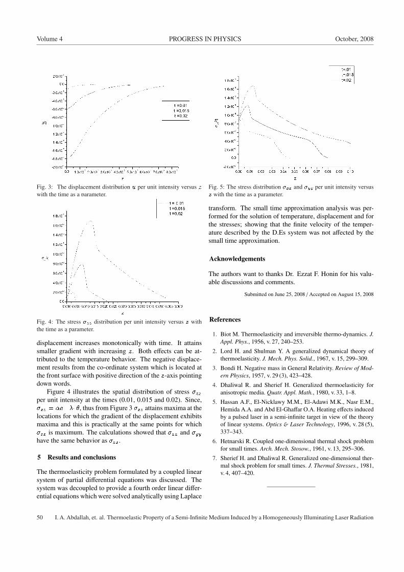
Volume 4 PROGRESS IN PHYSICS October, 2008
Fig. 3: The displacement distribution u per unit intensity versus zwith the time as a parameter.
Fig. 4: The stress �zz distribution per unit intensity versus z withthe time as a parameter.
displacement increases monotonically with time. It attainssmaller gradient with increasing z. Both effects can be at-tributed to the temperature behavior. The negative displace-ment results from the co-ordinate system which is located atthe front surface with positive direction of the z-axis pointingdown words.
Figure 4 illustrates the spatial distribution of stress �zzper unit intensity at the times (0.01, 0.015 and 0.02). Since,�zz = �e��1�, thus from Figure 3 �zz attains maxima at thelocations for which the gradient of the displacement exhibitsmaxima and this is practically at the same points for which�zz is maximum. The calculations showed that �xx and �yyhave the same behavior as �zz .
5 Results and conclusions
The thermoelasticity problem formulated by a coupled linearsystem of partial differential equations was discussed. Thesystem was decoupled to provide a fourth order linear differ-ential equations which were solved analytically using Laplace
Fig. 5: The stress distribution �xx and �yy per unit intensity versusz with the time as a parameter.
transform. The small time approximation analysis was per-formed for the solution of temperature, displacement and forthe stresses; showing that the finite velocity of the temper-ature described by the D.Es system was not affected by thesmall time approximation.
Acknowledgements
The authors want to thanks Dr. Ezzat F. Honin for his valu-able discussions and comments.
Submitted on June 25, 2008 / Accepted on August 15, 2008
References
1. Biot M. Thermoelasticity and irreversible thermo-dynamics. J.Appl. Phys., 1956, v. 27, 240–253.
2. Lord H. and Shulman Y. A generalized dynamical theory ofthermoelasticity. J. Mech. Phys. Solid., 1967, v. 15, 299–309.
3. Bondi H. Negative mass in General Relativity. Review of Mod-ern Physics, 1957, v. 29 (3), 423–428.
4. Dhaliwal R. and Sherief H. Generalized thermoelasticity foranisotropic media. Quatr. Appl. Math., 1980, v. 33, 1–8.
5. Hassan A.F., El-Nicklawy M.M., El-Adawi M.K., Nasr E.M.,Hemida A.A. and Abd El-Ghaffar O.A. Heating effects inducedby a pulsed laser in a semi-infinite target in view of the theoryof linear systems. Optics & Laser Technology, 1996, v. 28 (5),337–343.
6. Hetnarski R. Coupled one-dimensional thermal shock problemfor small times. Arch. Mech. Stosow., 1961, v. 13, 295–306.
7. Sherief H. and Dhaliwal R. Generalized one-dimensional ther-mal shock problem for small times. J. Thermal Stresses., 1981,v. 4, 407–420.
50 I. A. Abdallah, et. al. Thermoelastic Property of a Semi-Infinite Medium Induced by a Homogeneously Illuminating Laser Radiation
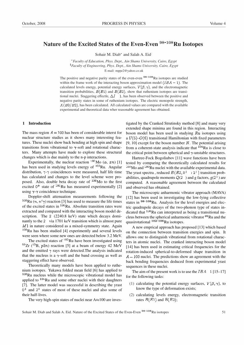
October, 2008 PROGRESS IN PHYSICS Volume 4
Nature of the Excited States of the Even-Even 98-108Ru Isotopes
Sohair M. Diab� and Salah A. Eidy�Faculty of Education, Phys. Dept., Ain Shams University, Cairo, EgyptyFaculty of Engineering, Phys. Dept., Ain Shams University, Cairo, Egypt
E-mail: [email protected]
The positive and negative parity states of the even-even 98-108Ru isotopes are studiedwithin the frame work of the interacting boson approximation model (IBA � 1). Thecalculated levels energy, potential energy surfaces, V (�; ), and the electromagnetictransition probabilities, B(E1) and B(E2), show that ruthenium isotopes are transi-tional nuclei. Staggering effectle, �I = 1, has been observed between the positive andnegative parity states in some of ruthenium isotopes. The electric monopole strength,X(E0=E2), has been calculated. All calculated values are compared with the availableexperimental and theoretical data wher reasonable agreement has obtained.
1 Introduction
The mass region A= 100 has been of considerable interst fornuclear structure studies as it shows many interesting fea-tures. These nuclei show back bending at high spin and shapetransitions from vibrational to -soft and rotational charac-ters. Many attempts have made to explore these structuralchanges which is due mainly to the n-p interactions.
Experimentally, the nuclear reaction 100Mo (�, xn) [1]has been used in studying levels energy of 100Ru. Angulardistribution, - coincidences were measured, half life timehas calculated and changes to the level scheme were pro-posed. Also, double beta decay rate of 100Mo to the firstexcited 0+ state of 100Ru has measured experimentally [2]using - coincidence technique.
Doppler-shift attenuation measurements following the100Ru (n, n` ) reaction [3] has used to measure the life timesof the excited states in 100Ru. Absolute transition rates wereextracted and compared with the interacting boson model de-scription. The 2+(2240.8 keV) state which decays domi-nantly to the 2+ via 1701 keV transition which is almost pureM1 in nature considered as a mixed-symmetry state. Again100Ru has been studied [4] experimently and several levelswere seen where some new ones are detected below 3.2 MeV.
The excited states of 102Ru have been investigated using96Zr (10B, p3n) reaction [5] at a beam of energy 42 MeVand the emitted rays were detected.The analysis indicatedthat the nucleus is a -soft and the band crossing as well asstaggering effect have observed.
Theoretically many models have been applied to ruthe-nium isotopes. Yukawa folded mean field [6] has applied to100Ru nucleus while the microscopic vibrational model hasapplied to 104Ru and some other nuclei with their daughters[7]. The latter model was successful in describing the yrast0+ and 2+ states of most of these nuclei and also some oftheir half-lives.
The very high-spin states of nuclei near A�100 are inves-
tigated by the Cranked Strutinsky method [8] and many veryextended shape minima are found in this region. Interactingboson model has been used in studying Ru isotopes usinga U(5)–O(6) transitional Hamiltonian with fixed parameters[9, 10] except for the boson number N . The potential arisingfrom a coherent-state analysis indicate that 104Ru is close tothe critical point between spherical and -unstable structures.
Hartree-Fock Bogoliubov [11] wave functions have beentested by comparing the theoretically calculated results for100Mo and 100Ru nuclei with the available experimental data.The yrast spectra , reduced B (E2; 0+! 2+) transition prob-abilities, quadrupole momentsQ(2+) and g factors, g(2+) arecomputed. A reasonable agreement between the calculatedand observed has obtained.
The microscopic anharmonic vibrator approach (MAVA)[12] has been used in investigating the low-lying collectivestates in 98-108Ru. Analysis for the level energies and elec-tric quadrupole decays of the two-phonon type of states in-dicated that 100Ru can interpreted as being a transitional nu-cleus between the spherical anharmonic vibrator 98Ru and thequasirotational 102-106Ru isotopes.
A new emprical approach has proposed [13] which basedon the connection between transition energies and spin. Itallows one to distinguish vibrational from rotational charac-ters in atomic nuclei. The cranked interacting boson model[14] has been used in estimating critical frequencies for therotation-induced spherical-to-deformed shape transition inA= 100 nuclei. The predictions show an agreement with theback bending frequencies deduced from experimental yrastsequences in these nuclei.
The aim of the present work is to use the IBA�1 [15–17]for the following tasks:
(1) calculating the potential energy surfaces, V (�; ), toknow the type of deformation exists;
(2) calculating levels energy, electromagnetic transitionrates B(E1) and B(E2);
Sohair M. Diab and Salah A. Eid. Nature of the Excited States of the Even-Even 98-108Ru isotopes 51
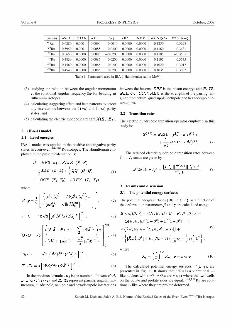
Volume 4 PROGRESS IN PHYSICS October, 2008
nucleus EPS PAIR ELL QQ OCT HEX E2SD(eb) E2DD(eb)98Ru 0.6280 0.000 0.0090 �0.0010 0.0000 0.0000 0.1250 �0.3698100Ru 0.5950 0.000 0.0085 �0.0200 0.0000 0.0000 0.1160 �0.3431102Ru 0.5650 0.0000 0.0085 �0.0200 0.0000 0.0000 0.1185 �0.3505104Ru 0.4830 0.0000 0.0085 �0.0200 0.0000 0.0000 0.1195 �0.3535106Ru 0.4560 0.0000 0.0085 �0.0200 0.0000 0.0000 0.1020 �0.3017108Ru 0.4540 0.0000 0.0085 �0.0200 0.0000 0.0000 0.1035 �0.3062
Table 1: Parameters used in IBA-1 Hamiltonian (all in MeV).
(3) studying the relation between the angular momentumI , the rotational angular frequency ~! for bending inruthenium isotopes;
(4) calculating staggering effect and beat patterns to detectany interactions between the (+ve) and (�ve) paritystates; and
(5) calculating the electric monopole strengthX(E0=E2).
2 (IBA-1) model
2.1 Level energies
IBA-1 model was applied to the positive and negative paritystates in even-even 98-108Ru isotopes. The Hamiltonian em-ployed in the present calculation is:
H = EPS � nd + PAIR � (P � P )
+12ELL � (L � L) +
12QQ � (Q �Q)
+ 5OCT � (T3 � T3) + 5HEX � (T4 � T4) ;
(1)
where
P � p =12
24 n(sysy)(0)0 �
p5(dydy)(0)
0
oxn
(ss)(0)0 �
p5( ~d ~d)(0)
0
o 35(0)
0
; (2)
L � L = �10p
3h(dy ~d)(1)x (dy ~d)(1)
i(0)
0; (3)
Q �Q =p
5
26664�
(Sy ~d+ dys)(2) �p
72
(dy ~d)(2)�x�
(sy ~d+ + ~ds)(2) �p
72
(dy ~d)(2)�37775
(0)
0
; (4)
T3 � T3 = �p7h(dy ~d)(2)x (dy ~d)(2)
i(0)
0; (5)
T4 � T4 = 3h(dy ~d)(4)x (dy ~d)(4)
i(0)
0: (6)
In the previous formulas, nd is the number of boson; P �P ,L �L, Q �Q, T3 �T3 and T4 �T4 represent pairing, angular mo-mentum, quadrupole, octupole and hexadecupole interactions
between the bosons; EPS is the boson energy; and PAIR,ELL, QQ, OCT , HEX is the strengths of the pairing, an-gular momentum, quadrupole, octupole and hexadecupole in-teractions.
2.2 Transition rates
The electric quadrupole transition operator employed in thisstudy is:
T (E2) = E2SD � (sy ~d+ dys)(2) +
+1p5E2DD � (dy ~d)(2) : (7)
The reduced electric quadrupole transition rates betweenIi ! If states are given by
B (E2; Ii � If ) =[< If k T (E2) k Ii >]2
2Ii + 1: (8)
3 Results and discussion
3.1 The potential energy surfaces
The potential energy surfaces [18], V (�, ), as a function ofthe deformation parameters � and are calculated using:
EN�N� (�; ) = <N�N� ;� jH�� jN�N� ;� > =
= �d(N�N�)�2(1 + �2) + �2(1 + �2)�2���kN�N�[4� ( �X� �X�)� cos 3 ]
+
+�
[ �X� �X��2] +N�(N� � 1)�
110c0 +
17c2��2�;
(9)
where
�X� =�
27
�0:5
X� � = � or � : (10)
The calculated potential energy surfaces, V (�; ), arepresented in Fig. 1. It shows that 98Ru is a vibrational —like nucleus while 100�104Ru are -soft where the two wellson the oblate and prolate sides are equal. 106;108Ru are rota-tional - like where they are prolate deformed.
52 Sohair M. Diab and Salah A. Eid. Nature of the Excited States of the Even-Even 98-108Ru Isotopes
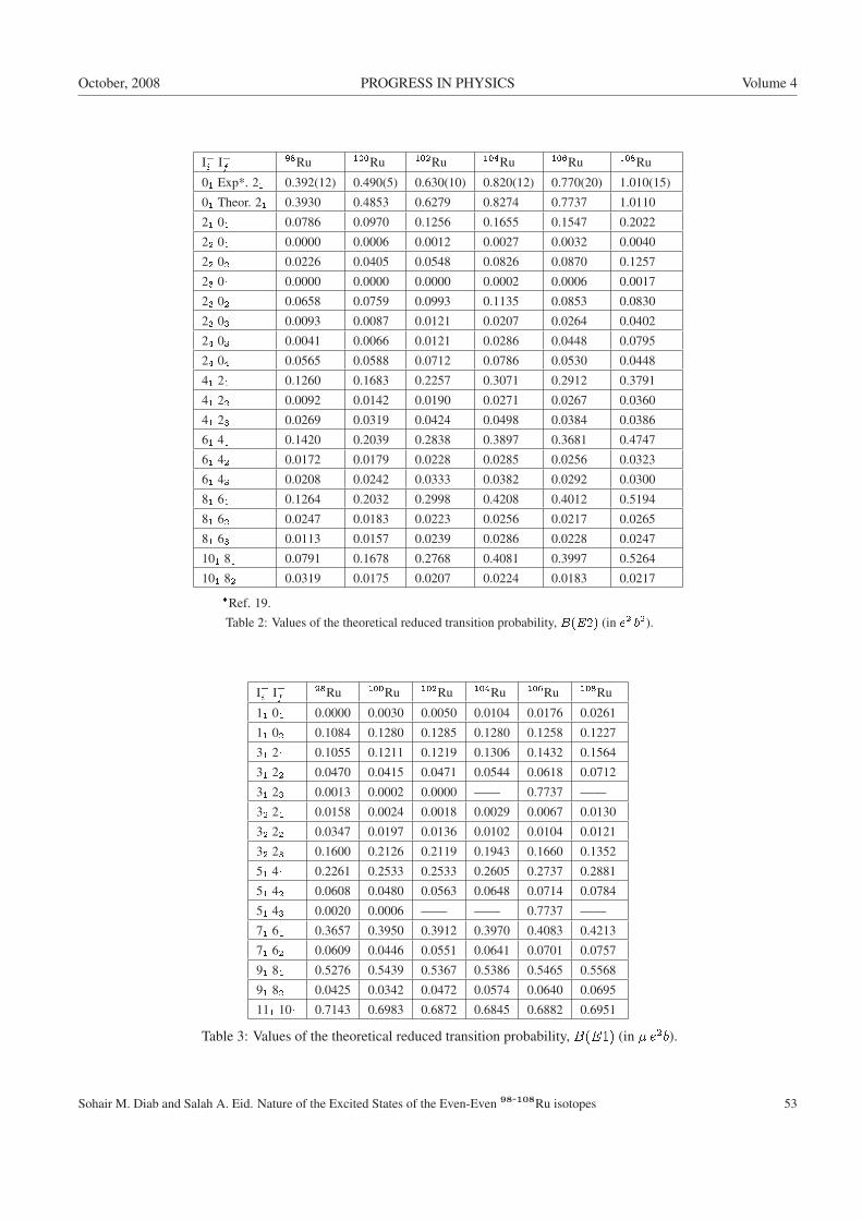
October, 2008 PROGRESS IN PHYSICS Volume 4
I+i I+f98Ru 100Ru 102Ru 104Ru 106Ru 108Ru
01 Exp*. 21 0.392(12) 0.490(5) 0.630(10) 0.820(12) 0.770(20) 1.010(15)
01 Theor. 21 0.3930 0.4853 0.6279 0.8274 0.7737 1.0110
21 01 0.0786 0.0970 0.1256 0.1655 0.1547 0.2022
22 01 0.0000 0.0006 0.0012 0.0027 0.0032 0.0040
22 02 0.0226 0.0405 0.0548 0.0826 0.0870 0.1257
23 01 0.0000 0.0000 0.0000 0.0002 0.0006 0.0017
23 02 0.0658 0.0759 0.0993 0.1135 0.0853 0.0830
23 03 0.0093 0.0087 0.0121 0.0207 0.0264 0.0402
24 03 0.0041 0.0066 0.0121 0.0286 0.0448 0.0795
24 04 0.0565 0.0588 0.0712 0.0786 0.0530 0.0448
41 21 0.1260 0.1683 0.2257 0.3071 0.2912 0.3791
41 22 0.0092 0.0142 0.0190 0.0271 0.0267 0.0360
41 23 0.0269 0.0319 0.0424 0.0498 0.0384 0.0386
61 41 0.1420 0.2039 0.2838 0.3897 0.3681 0.4747
61 42 0.0172 0.0179 0.0228 0.0285 0.0256 0.0323
61 43 0.0208 0.0242 0.0333 0.0382 0.0292 0.0300
81 61 0.1264 0.2032 0.2998 0.4208 0.4012 0.5194
81 62 0.0247 0.0183 0.0223 0.0256 0.0217 0.0265
81 63 0.0113 0.0157 0.0239 0.0286 0.0228 0.0247
101 81 0.0791 0.1678 0.2768 0.4081 0.3997 0.5264
101 82 0.0319 0.0175 0.0207 0.0224 0.0183 0.0217�Ref. 19.Table 2: Values of the theoretical reduced transition probability, B(E2) (in e2 b2).
I+i I+f98Ru 100Ru 102Ru 104Ru 106Ru 108Ru
11 01 0.0000 0.0030 0.0050 0.0104 0.0176 0.0261
11 02 0.1084 0.1280 0.1285 0.1280 0.1258 0.1227
31 21 0.1055 0.1211 0.1219 0.1306 0.1432 0.1564
31 22 0.0470 0.0415 0.0471 0.0544 0.0618 0.0712
31 23 0.0013 0.0002 0.0000 —— 0.7737 ——
32 21 0.0158 0.0024 0.0018 0.0029 0.0067 0.0130
32 22 0.0347 0.0197 0.0136 0.0102 0.0104 0.0121
32 23 0.1600 0.2126 0.2119 0.1943 0.1660 0.1352
51 41 0.2261 0.2533 0.2533 0.2605 0.2737 0.2881
51 42 0.0608 0.0480 0.0563 0.0648 0.0714 0.0784
51 43 0.0020 0.0006 —— —— 0.7737 ——
71 61 0.3657 0.3950 0.3912 0.3970 0.4083 0.4213
71 62 0.0609 0.0446 0.0551 0.0641 0.0701 0.0757
91 81 0.5276 0.5439 0.5367 0.5386 0.5465 0.5568
91 82 0.0425 0.0342 0.0472 0.0574 0.0640 0.0695
111 101 0.7143 0.6983 0.6872 0.6845 0.6882 0.6951
Table 3: Values of the theoretical reduced transition probability, B(E1) (in � e2b).
Sohair M. Diab and Salah A. Eid. Nature of the Excited States of the Even-Even 98-108Ru isotopes 53
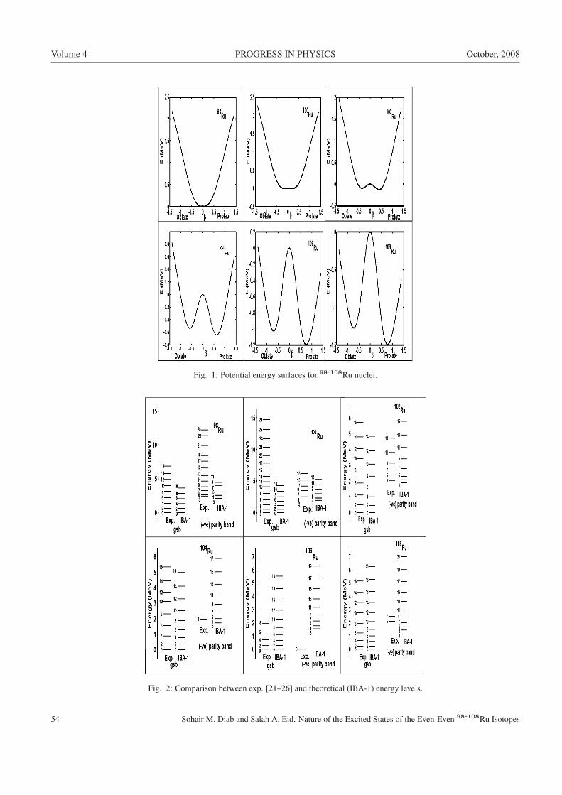
Volume 4 PROGRESS IN PHYSICS October, 2008
Fig. 1: Potential energy surfaces for 98-108Ru nuclei.
Fig. 2: Comparison between exp. [21–26] and theoretical (IBA-1) energy levels.
54 Sohair M. Diab and Salah A. Eid. Nature of the Excited States of the Even-Even 98-108Ru Isotopes
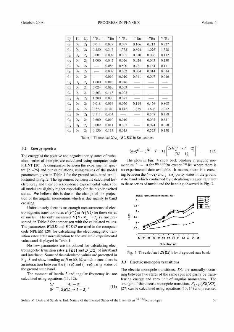
October, 2008 PROGRESS IN PHYSICS Volume 4
I+i I+f I+0f98Ru 100Ru 102Ru 104Ru 106Ru 108Ru
02 01 21 0.011 0.027 0.057 0.166 0.213 0.227
03 01 21 0.250 0.347 1.333 0.894 1.076 1.328
03 01 22 0.001 0.009 0.005 0.010 0.086 0.112
03 01 23 1.000 0.042 0.026 0.024 0.043 0.130
03 02 21 —– 0.086 0.500 0.421 0.184 0.171
03 02 22 —– 0.002 0.002 0.004 0.014 0.014
03 02 23 —– 0.010 0.010 0.011 0.007 0.016
04 01 22 1.600 0.010 0.046 —– —– —–
04 01 23 0.024 0.010 0.003 —– —– —–
04 01 24 0.363 0.113 0.003 —– —– —–
04 02 22 1.200 0.030 0.097 —– —– —–
04 02 23 0.018 0.034 0.070 0.114 0.476 0.808
04 02 24 0.272 0.340 0.142 1.035 3.696 2.082
04 03 21 0.111 0.454 —– —– 0.558 0.458
04 03 22 0.600 0.010 0.010 —– 0.002 0.611
04 03 23 0.009 0.011 0.007 —– 0.074 0.058
04 03 24 0.136 0.113 0.015 —– 0.575 0.150
Table 4. Theoretical Xif 0f (E0/E2) in Ru isotopes.
3.2 Energy spectra
The energy of the positive and negative parity states of ruthe-nium series of isotopes are calculated using computer codePHINT [20]. A comparison between the experimental spec-tra [21–26] and our calculations, using values of the modelparameters given in Table 1 for the ground state band are il-lustrated in Fig. 2. The agreement between the calculated lev-els energy and their correspondence experimental values forall nuclei are slightly higher especially for the higher excitedstates. We believe this is due to the change of the projec-tion of the angular momentum which is due mainly to bandcrossing.
Unfortunately there is no enough measurements of elec-tromagnetic transition ratesB (E1) orB (E2) for these seriesof nuclei. The only measured B (E2; 0+
1 ! 2+1 )’s are pre-
sented, in Table 2 for comparison with the calculated values.The parameters E2SD and E2DD are used in the computercode NPBEM [20] for calculating the electromagnetic tran-sition rates after normalization to the available experimentalvalues and displayed in Table 1.
No new parameters are introduced for calculating elec-tromagnetic transition rates B (E1) and B (E2) of intrabandand interband. Some of the calculated values are presented inFig. 3 and show bending at N = 60, 62 which means there isan interaction between the (+ve) and (�ve) parity states ofthe ground state band.
The moment of inertia I and angular frequency ~! arecalculated using equations (11, 12):
2I~2 =
4I � 2�E(I ! I � 2)
; (11)
(~!)2 = (I2 � I + 1)�
�E(I ! I � 2)(2I � 1)
�2
: (12)
The plots in Fig. 4 show back bending at angular mo-mentum I+ = 10 for 98-108Ru except 106Ru where there isno experimental data available. It means, there is a cross-ing between the (+ve) and (�ve) parity states in the groundstate band which confirmed by calculating staggering effectto these series of nuclei and the bending observed in Fig. 3.
Fig. 3: The calculated B(E2)’s for the ground state band.
3.3 Electric monopole transitions
The electric monopole transitions, E0, are normally occur-ring between two states of the same spin and parity by trans-ferring energy and zero unit of angular momentum. Thestrength of the electric monopole transition, Xif 0f (E0=E2),[27] can be calculated using equations (13, 14) and presented
Sohair M. Diab and Salah A. Eid. Nature of the Excited States of the Even-Even 98-108Ru isotopes 55
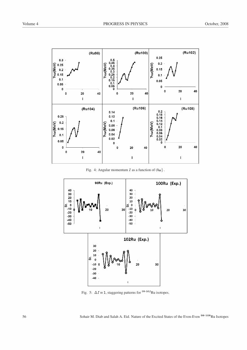
Volume 4 PROGRESS IN PHYSICS October, 2008
Fig. 4: Angular momentum I as a function of (~!) .
Fig. 5: �I = 1, staggering patterns for 98-102Ru isotopes.
56 Sohair M. Diab and Salah A. Eid. Nature of the Excited States of the Even-Even 98-108Ru Isotopes
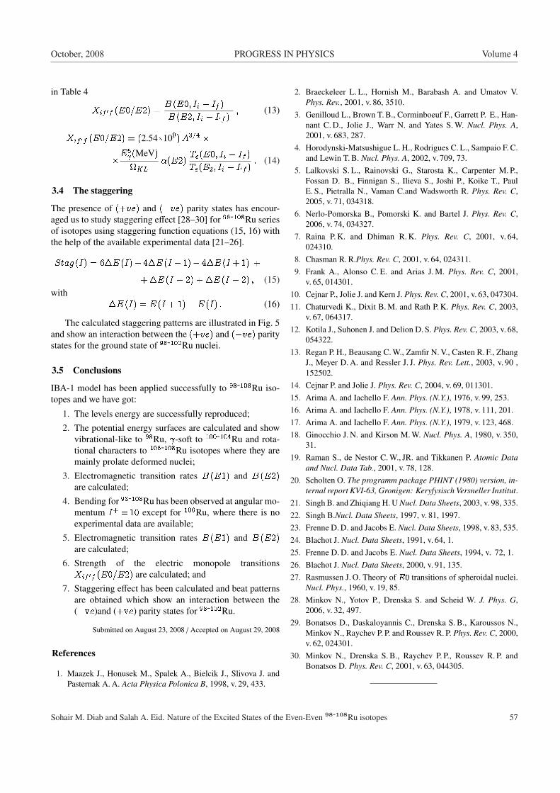
October, 2008 PROGRESS IN PHYSICS Volume 4
in Table 4
Xif 0f (E0=E2) =B (E0; Ii � If )B (E2; Ii � I0f )
; (13)
Xif 0f (E0=E2) = (2.54�109)A3=4 ��E
5 (MeV)KL
�(E2)Te(E0; Ii � If )Te(E2; Ii � I0f )
: (14)
3.4 The staggering
The presence of (+ve) and (�ve) parity states has encour-aged us to study staggering effect [28–30] for 98-108Ru seriesof isotopes using staggering function equations (15, 16) withthe help of the available experimental data [21–26].
Stag (I) = 6�E (I)� 4�E (I � 1)� 4�E (I + 1) +
+ �E (I + 2) + �E (I � 2) ; (15)with
�E (I) = E (I + 1)� E (I) : (16)
The calculated staggering patterns are illustrated in Fig. 5and show an interaction between the (+ve) and (�ve) paritystates for the ground state of 98-102Ru nuclei.
3.5 Conclusions
IBA-1 model has been applied successfully to 98-108Ru iso-topes and we have got:
1. The levels energy are successfully reproduced;2. The potential energy surfaces are calculated and show
vibrational-like to 98Ru, -soft to 100-104Ru and rota-tional characters to 106-108Ru isotopes where they aremainly prolate deformed nuclei;
3. Electromagnetic transition rates B (E1) and B (E2)are calculated;
4. Bending for 98-108Ru has been observed at angular mo-mentum I+ = 10 except for 106Ru, where there is noexperimental data are available;
5. Electromagnetic transition rates B (E1) and B (E2)are calculated;
6. Strength of the electric monopole transitionsXif 0f (E0=E2) are calculated; and
7. Staggering effect has been calculated and beat patternsare obtained which show an interaction between the(�ve)and (+ve) parity states for 98-102Ru.
Submitted on August 23, 2008 / Accepted on August 29, 2008
References
1. Maazek J., Honusek M., Spalek A., Bielcik J., Slivova J. andPasternak A. A. Acta Physica Polonica B, 1998, v. 29, 433.
2. Braeckeleer L. L., Hornish M., Barabash A. and Umatov V.Phys. Rev., 2001, v. 86, 3510.
3. Genilloud L., Brown T. B., Corminboeuf F., Garrett P. E., Han-nant C. D., Jolie J., Warr N. and Yates S. W. Nucl. Phys. A,2001, v. 683, 287.
4. Horodynski-Matsushigue L. H., Rodrigues C. L., Sampaio F. C.and Lewin T. B. Nucl. Phys. A, 2002, v. 709, 73.
5. Lalkovski S. L., Rainovski G., Starosta K., Carpenter M. P.,Fossan D. B., Finnigan S., Ilieva S., Joshi P., Koike T., PaulE. S., Pietralla N., Vaman C.and Wadsworth R. Phys. Rev. C,2005, v. 71, 034318.
6. Nerlo-Pomorska B., Pomorski K. and Bartel J. Phys. Rev. C,2006, v. 74, 034327.
7. Raina P. K. and Dhiman R. K. Phys. Rev. C, 2001, v. 64,024310.
8. Chasman R. R.Phys. Rev. C, 2001, v. 64, 024311.9. Frank A., Alonso C. E. and Arias J. M. Phys. Rev. C, 2001,
v. 65, 014301.10. Cejnar P., Jolie J. and Kern J. Phys. Rev. C, 2001, v. 63, 047304.11. Chaturvedi K., Dixit B. M. and Rath P. K. Phys. Rev. C, 2003,
v. 67, 064317.12. Kotila J., Suhonen J. and Delion D. S. Phys. Rev. C, 2003, v. 68,
054322.13. Regan P. H., Beausang C. W., Zamfir N. V., Casten R. F., Zhang
J., Meyer D. A. and Ressler J. J. Phys. Rev. Lett., 2003, v. 90 ,152502.
14. Cejnar P. and Jolie J. Phys. Rev. C, 2004, v. 69, 011301.15. Arima A. and Iachello F. Ann. Phys. (N.Y.), 1976, v. 99, 253.16. Arima A. and Iachello F. Ann. Phys. (N.Y.), 1978, v. 111, 201.17. Arima A. and Iachello F. Ann. Phys. (N.Y.), 1979, v. 123, 468.18. Ginocchio J. N. and Kirson M. W. Nucl. Phys. A, 1980, v. 350,
31.19. Raman S., de Nestor C. W., JR. and Tikkanen P. Atomic Data
and Nucl. Data Tab., 2001, v. 78, 128.20. Scholten O. The programm package PHINT (1980) version, in-
ternal report KVI-63, Gronigen: Keryfysisch Versneller Institut.21. Singh B. and Zhiqiang H. U Nucl. Data Sheets, 2003, v. 98, 335.22. Singh B.Nucl. Data Sheets, 1997, v. 81, 1997.23. Frenne D. D. and Jacobs E. Nucl. Data Sheets, 1998, v. 83, 535.24. Blachot J. Nucl. Data Sheets, 1991, v. 64, 1.25. Frenne D. D. and Jacobs E. Nucl. Data Sheets, 1994, v. 72, 1.26. Blachot J. Nucl. Data Sheets, 2000, v. 91, 135.27. Rasmussen J. O. Theory of E0 transitions of spheroidal nuclei.
Nucl. Phys., 1960, v. 19, 85.28. Minkov N., Yotov P., Drenska S. and Scheid W. J. Phys. G,
2006, v. 32, 497.29. Bonatsos D., Daskaloyannis C., Drenska S. B., Karoussos N.,
Minkov N., Raychev P. P. and Roussev R. P. Phys. Rev. C, 2000,v. 62, 024301.
30. Minkov N., Drenska S. B., Raychev P. P., Roussev R. P. andBonatsos D. Phys. Rev. C, 2001, v. 63, 044305.
Sohair M. Diab and Salah A. Eid. Nature of the Excited States of the Even-Even 98-108Ru isotopes 57
Progress in Physicsis an American scientific journal on advanced stud-ies in physics, registered with the Library of Congress (DC,USA): ISSN1555-5534 (print version) and ISSN 1555-5615 (online version). The jour-nal is peer reviewed and listed in the abstracting and indexing coverageof: Mathematical Reviews of the AMS (USA), DOAJ of Lund Univer-sity (Sweden), Zentralblatt MATH (Germany), Scientific Commons of theUniversity of St. Gallen (Switzerland), Open-J-Gate (India), ReferentialJournal of VINITI (Russia), etc. Progress in Physicsis an open-accessjournal published and distributed in accordance with the Budapest OpenInitiative: this means that the electronic copies of both full-size versionof the journal and the individual papers published therein will always beacessed for reading, download, and copying for any user freeof charge.The journal is issued quarterly (four volumes per year).
Electronic version of this journal:http: //www.ptep-online.com
Editorial board:
Dmitri Rabounski (Editor-in-Chief)Florentin SmarandacheLarissa BorissovaStephen J. Crothers
Postal address for correspondence:
Department of Mathematics and ScienceUniversity of New Mexico200 College Road, Gallup, NM 87301, USA
Printed in the United States of America