Embed Size (px)
Citation preview

Progress in MathematicsVolume 236
Series EditorsHyman BassJoseph OesterleAlan Weinstein

Ryoshi Hotta
Kiyoshi Takeuchi
Toshiyuki Tanisaki
D-Modules,Perverse Sheaves,and Representation TheoryTranslated byKiyoshi Takeuchi
BirkhauserBoston • Basel • Berlin

Ryoshi HottaProfessor Emeritus of Tohoku UniversityShirako 2-25-1-1106Wako [email protected]
Kiyoshi TakeuchiSchool of MathematicsTsukuba UniversityTenoudai 1-1-1Tsukuba [email protected]
Toshiyuki TanisakiDepartment of MathematicsGraduate School of ScienceOsaka City University3-3-138 SugimotoSumiyoshi-kuOsaka [email protected]
Mathematics Subject Classification (2000): Primary: 32C38, 20G05; Secondary: 32S35, 32S60, 17B10
Library of Congress Control Number: 2004059581
ISBN-13: 978-0-8176-4363-8 e-ISBN-13: 978-0-8176-4523-6
Printed on acid-free paper.
c 2008, English Edition Birkhauser Bostonc 1995, Japanese Edition, Springer-Verlag Tokyo, D Kagun to Daisugun (D-Modules and AlgebraicGroups) by R. Hotta and T. Tanisaki.
All rights reserved. This work may not be translated or copied in whole or in part without the writ-ten permission of the publisher (Birkhauser Boston, c/o Springer Science Business Media LLC, 233Spring Street, New York, NY 10013, USA), except for brief excerpts in connection with reviews orscholarly analysis. Use in connection with any form of information storage and retrieval, electronicadaptation, computer software, or by similar or dissimilar methodology now known or hereafter de-veloped is forbidden.The use in this publication of trade names, trademarks, service marks and similar terms, even if theyare not identified as such, is not to be taken as an expression of opinion as to whether or not they aresubject to proprietary rights.
9 8 7 6 5 4 3 2 1
www.birkhauser.com (JLS/SB)
Preface
D-Modules, Perverse Sheaves, and Representation Theory is a greatly expandedtranslation of the Japanese edition entitled D kagun to daisugun (D-Modules andAlgebraic Groups) which was published by Springer-Verlag Tokyo, 1995. For thenew English edition, the two authors of the original book, R. Hotta and T. Tanisaki,have added K. Takeuchi as a coauthor. Significant new material along with correctionsand modifications have been made to this English edition.
In the summer of 1982, a symposium was held in Kinosaki in which the sub-ject of D-modules and their applications to representation theory was introduced.At that time the theory of regular holonomic D-modules had just been completedand the Kazhdan–Lusztig conjecture had been settled by Brylinski–Kashiwara andBeilinson–Bernstein. The articles that appeared in the published proceedings of thesymposium were not well presented and of course the subject was still in its infancy.Several monographs, however, did appear later on D-modules, for example, Björk[Bj2], Borel et al. [Bor3], Kashiwara–Schapira [KS2], Mebkhout [Me5] and others,all of which were taken into account and helped us make our Japanese book morecomprehensive and readable. In particular, J. Bernstein’s notes [Ber1] were extremelyuseful to understand the subject in the algebraic case; our treatment in many aspectsfollows the method used in the notes. Our plan was to present the combination ofD-module theory and its typical applications to representation theory as we believethat this is a nice way to understand the whole subject.
Let us briefly explain the contents of this book. Part I is devoted to D-moduletheory, placing special emphasis on holonomic modules and constructible sheaves.The aim here is to present a proof of the Riemann–Hilbert correspondence. Part IIis devoted to representation theory. In particular, we will explain how the Kazhdan–Lusztig conjecture was solved using the theory of D-modules. To a certain extent weassume the reader’s familiarity with algebraic geometry, homological algebras, andsheaf theory. Although we include in the appendices brief introductions to algebraicvarieties and derived categories, which are sufficient overall for dealing with the text,the reader should occasionally refer to appropriate references mentioned in the text.
The main difference from the original Japanese edition is that we made some newchapters and sections for analytic D-modules, meromorphic connections, perverse

vi Preface
sheaves, and so on. We thus emphasized the strong connections of D-modules withvarious other fields of mathematics.
We express our cordial thanks to A. D’Agnolo, C. Marastoni, Y. Matsui,P. Schapira, and J. Schürmann for reading very carefully the draft of the Englishversion and giving us many valuable comments. Discussions with M. Kaneda,K. Kimura, S. Naito, J.-P. Schneiders, K. Vilonen, and others were also very helpfulin completing the exposition. M. Nagura and Y. Sugiki greatly helped us in typingand correcting our manuscript. Thanks also go to many people for useful commentson our Japanese version, in particular to T. Ohsawa. Last but not least, we cannot ex-aggerate our gratitude to M. Kashiwara throughout the period since 1980 on variousoccasions.
2006 March R. Hotta
K. TakeuchiCollege of Mathematics, University of Tsukuba
T. TanisakiFaculty of Science, Osaka City University
Contents
Preface . . . . . . . . . . . . . . . . . . . . . . . . . . . . . . . . . . . . . . . . . . . . . . . . . . . . . . . . . v
Introduction . . . . . . . . . . . . . . . . . . . . . . . . . . . . . . . . . . . . . . . . . . . . . . . . . . . . . 1
Part I D-Modules and Perverse Sheaves
1 Preliminary Notions . . . . . . . . . . . . . . . . . . . . . . . . . . . . . . . . . . . . . . . . . . 151.1 Differential operators . . . . . . . . . . . . . . . . . . . . . . . . . . . . . . . . . . . . . . . 151.2 D-modules—warming up . . . . . . . . . . . . . . . . . . . . . . . . . . . . . . . . . . . . 171.3 Inverse and direct images I . . . . . . . . . . . . . . . . . . . . . . . . . . . . . . . . . . . 211.4 Some categories of D-modules . . . . . . . . . . . . . . . . . . . . . . . . . . . . . . . 251.5 Inverse images and direct images II . . . . . . . . . . . . . . . . . . . . . . . . . . . 311.6 Kashiwara’s equivalence . . . . . . . . . . . . . . . . . . . . . . . . . . . . . . . . . . . . 481.7 A base change theorem for direct images . . . . . . . . . . . . . . . . . . . . . . . 53
2 Coherent D-Modules . . . . . . . . . . . . . . . . . . . . . . . . . . . . . . . . . . . . . . . . . 572.1 Good filtrations . . . . . . . . . . . . . . . . . . . . . . . . . . . . . . . . . . . . . . . . . . . . 572.2 Characteristic varieties (singular supports) . . . . . . . . . . . . . . . . . . . . . . 592.3 Dimensions of characteristic varieties . . . . . . . . . . . . . . . . . . . . . . . . . . 622.4 Inverse images in the non-characteristic case . . . . . . . . . . . . . . . . . . . . 642.5 Proper direct images . . . . . . . . . . . . . . . . . . . . . . . . . . . . . . . . . . . . . . . . 692.6 Duality functors . . . . . . . . . . . . . . . . . . . . . . . . . . . . . . . . . . . . . . . . . . . . 702.7 Relations among functors . . . . . . . . . . . . . . . . . . . . . . . . . . . . . . . . . . . . 76
2.7.1 Duality functors and inverse images . . . . . . . . . . . . . . . . . . . . 762.7.2 Duality functors and direct images . . . . . . . . . . . . . . . . . . . . . . 77
3 Holonomic D-Modules . . . . . . . . . . . . . . . . . . . . . . . . . . . . . . . . . . . . . . . . 813.1 Basic results . . . . . . . . . . . . . . . . . . . . . . . . . . . . . . . . . . . . . . . . . . . . . . . 813.2 Functors for holonomic D-modules . . . . . . . . . . . . . . . . . . . . . . . . . . . 83
3.2.1 Stability of holonomicity . . . . . . . . . . . . . . . . . . . . . . . . . . . . . . 83
viii Contents
3.2.2 Holonomicity of modules over Weyl algebras . . . . . . . . . . . . 863.2.3 Adjunction formulas . . . . . . . . . . . . . . . . . . . . . . . . . . . . . . . . . . 91
3.3 Finiteness property . . . . . . . . . . . . . . . . . . . . . . . . . . . . . . . . . . . . . . . . . 933.4 Minimal extensions . . . . . . . . . . . . . . . . . . . . . . . . . . . . . . . . . . . . . . . . . 95
4 Analytic D-Modules and the de Rham Functor . . . . . . . . . . . . . . . . . . . 994.1 Analytic D-modules . . . . . . . . . . . . . . . . . . . . . . . . . . . . . . . . . . . . . . . . 994.2 Solution complexes and de Rham functors . . . . . . . . . . . . . . . . . . . . . . 1034.3 Cauchy–Kowalevski–Kashiwara theorem . . . . . . . . . . . . . . . . . . . . . . 1054.4 Cauchy problems and micro-supports . . . . . . . . . . . . . . . . . . . . . . . . . . 1074.5 Constructible sheaves . . . . . . . . . . . . . . . . . . . . . . . . . . . . . . . . . . . . . . . 1104.6 Kashiwara’s constructibility theorem . . . . . . . . . . . . . . . . . . . . . . . . . . 1134.7 Analytic D-modules associated to algebraic D-modules . . . . . . . . . . 119
5 Theory of Meromorphic Connections . . . . . . . . . . . . . . . . . . . . . . . . . . . . 1275.1 Meromorphic connections in the one-dimensional case . . . . . . . . . . . 127
5.1.1 Systems of ODEs and meromorphic connections . . . . . . . . . . 1275.1.2 Meromorphic connections with regular singularities . . . . . . . 1305.1.3 Regularity of D-modules on algebraic curves . . . . . . . . . . . . . 135
5.2 Regular meromorphic connections on complex manifolds . . . . . . . . . 1395.2.1 Meromorphic connections in higher dimensions . . . . . . . . . . 1395.2.2 Meromorphic connections with logarithmic poles . . . . . . . . . 1435.2.3 Deligne’s Riemann–Hilbert correspondence . . . . . . . . . . . . . . 147
5.3 Regular integrable connections on algebraic varieties . . . . . . . . . . . . . 153
6 Regular Holonomic D-Modules . . . . . . . . . . . . . . . . . . . . . . . . . . . . . . . . 1616.1 Definition and main theorems . . . . . . . . . . . . . . . . . . . . . . . . . . . . . . . . 1616.2 Proof of main theorems . . . . . . . . . . . . . . . . . . . . . . . . . . . . . . . . . . . . . 163
7 Riemann–Hilbert Correspondence . . . . . . . . . . . . . . . . . . . . . . . . . . . . . . 1717.1 Commutativity with de Rham functors . . . . . . . . . . . . . . . . . . . . . . . . . 1717.2 Riemann–Hilbert correspondence . . . . . . . . . . . . . . . . . . . . . . . . . . . . . 1747.3 Comparison theorem . . . . . . . . . . . . . . . . . . . . . . . . . . . . . . . . . . . . . . . . 178
8 Perverse Sheaves . . . . . . . . . . . . . . . . . . . . . . . . . . . . . . . . . . . . . . . . . . . . . 1818.1 Theory of perverse sheaves . . . . . . . . . . . . . . . . . . . . . . . . . . . . . . . . . . 181
8.1.1 t-structures . . . . . . . . . . . . . . . . . . . . . . . . . . . . . . . . . . . . . . . . . 1818.1.2 Perverse sheaves . . . . . . . . . . . . . . . . . . . . . . . . . . . . . . . . . . . . . 191
8.2 Intersection cohomology theory . . . . . . . . . . . . . . . . . . . . . . . . . . . . . . 2028.2.1 Introduction . . . . . . . . . . . . . . . . . . . . . . . . . . . . . . . . . . . . . . . . . 2028.2.2 Minimal extensions of perverse sheaves . . . . . . . . . . . . . . . . . 203
8.3 Hodge modules . . . . . . . . . . . . . . . . . . . . . . . . . . . . . . . . . . . . . . . . . . . . 2178.3.1 Motivation . . . . . . . . . . . . . . . . . . . . . . . . . . . . . . . . . . . . . . . . . . 2178.3.2 Hodge structures and their variations . . . . . . . . . . . . . . . . . . . . 2178.3.3 Hodge modules . . . . . . . . . . . . . . . . . . . . . . . . . . . . . . . . . . . . . . 220
Contents ix
Part II Representation Theory
9 Algebraic Groups and Lie Algebras . . . . . . . . . . . . . . . . . . . . . . . . . . . . . 2299.1 Lie algebras and their enveloping algebras . . . . . . . . . . . . . . . . . . . . . . 2299.2 Semisimple Lie algebras (1) . . . . . . . . . . . . . . . . . . . . . . . . . . . . . . . . . . 2319.3 Root systems . . . . . . . . . . . . . . . . . . . . . . . . . . . . . . . . . . . . . . . . . . . . . . 2339.4 Semisimple Lie algebras (2) . . . . . . . . . . . . . . . . . . . . . . . . . . . . . . . . . . 2369.5 Finite-dimensional representations of semisimple Lie algebras . . . . . 2399.6 Algebraic groups and their Lie algebras . . . . . . . . . . . . . . . . . . . . . . . . 2419.7 Semisimple algebraic groups . . . . . . . . . . . . . . . . . . . . . . . . . . . . . . . . . 2439.8 Representations of semisimple algebraic groups . . . . . . . . . . . . . . . . . 2489.9 Flag manifolds . . . . . . . . . . . . . . . . . . . . . . . . . . . . . . . . . . . . . . . . . . . . . 2509.10 Equivariant vector bundles . . . . . . . . . . . . . . . . . . . . . . . . . . . . . . . . . . . 2539.11 The Borel–Weil–Bott theorem . . . . . . . . . . . . . . . . . . . . . . . . . . . . . . . . 255
10 Conjugacy Classes of Semisimple Lie Algebras . . . . . . . . . . . . . . . . . . . . 25910.1 The theory of invariant polynomials . . . . . . . . . . . . . . . . . . . . . . . . . . . 25910.2 Classification of conjugacy classes . . . . . . . . . . . . . . . . . . . . . . . . . . . . 26310.3 Geometry of conjugacy classes . . . . . . . . . . . . . . . . . . . . . . . . . . . . . . . 266
11 Representations of Lie Algebras and D-Modules . . . . . . . . . . . . . . . . . . 27111.1 Universal enveloping algebras and differential operators . . . . . . . . . . 27111.2 Rings of twisted differential operators on flag varieties . . . . . . . . . . . 27211.3 Proof of Theorem 11.2.2 . . . . . . . . . . . . . . . . . . . . . . . . . . . . . . . . . . . . . 27611.4 Proof of Theorems 11.2.3 and 11.2.4 . . . . . . . . . . . . . . . . . . . . . . . . . . 28011.5 Equivariant representations and equivariant D-modules . . . . . . . . . . 28311.6 Classification of equivariant D-modules . . . . . . . . . . . . . . . . . . . . . . . 286
12 Character Formula of Highest Weight Modules . . . . . . . . . . . . . . . . . . . 28912.1 Highest weight modules . . . . . . . . . . . . . . . . . . . . . . . . . . . . . . . . . . . . . 28912.2 Kazhdan–Lusztig conjecture . . . . . . . . . . . . . . . . . . . . . . . . . . . . . . . . . 29512.3 D-modules associated to highest weight modules . . . . . . . . . . . . . . . . 299
13 Hecke Algebras and Hodge Modules . . . . . . . . . . . . . . . . . . . . . . . . . . . . 30513.1 Weyl groups and D-modules . . . . . . . . . . . . . . . . . . . . . . . . . . . . . . . . . 30513.2 Hecke algebras and Hodge modules . . . . . . . . . . . . . . . . . . . . . . . . . . . 310
A Algebraic Varieties . . . . . . . . . . . . . . . . . . . . . . . . . . . . . . . . . . . . . . . . . . . 321A.1 Basic definitions . . . . . . . . . . . . . . . . . . . . . . . . . . . . . . . . . . . . . . . . . . . 321A.2 Affine varieties . . . . . . . . . . . . . . . . . . . . . . . . . . . . . . . . . . . . . . . . . . . . . 323A.3 Algebraic varieties . . . . . . . . . . . . . . . . . . . . . . . . . . . . . . . . . . . . . . . . . . 325A.4 Quasi-coherent sheaves . . . . . . . . . . . . . . . . . . . . . . . . . . . . . . . . . . . . . 326A.5 Smoothness, dimensions and local coordinate systems . . . . . . . . . . . . 328

x Contents
B Derived Categories and Derived Functors . . . . . . . . . . . . . . . . . . . . . . . . 331B.1 Motivation . . . . . . . . . . . . . . . . . . . . . . . . . . . . . . . . . . . . . . . . . . . . . . . . 331B.2 Categories of complexes . . . . . . . . . . . . . . . . . . . . . . . . . . . . . . . . . . . . . 333B.3 Homotopy categories . . . . . . . . . . . . . . . . . . . . . . . . . . . . . . . . . . . . . . . 335B.4 Derived categories . . . . . . . . . . . . . . . . . . . . . . . . . . . . . . . . . . . . . . . . . . 339B.5 Derived functors . . . . . . . . . . . . . . . . . . . . . . . . . . . . . . . . . . . . . . . . . . . 343B.6 Bifunctors in derived categories . . . . . . . . . . . . . . . . . . . . . . . . . . . . . . 347
C Sheaves and Functors in Derived Categories . . . . . . . . . . . . . . . . . . . . . . 351C.1 Sheaves and functors . . . . . . . . . . . . . . . . . . . . . . . . . . . . . . . . . . . . . . . 351C.2 Functors in derived categories of sheaves . . . . . . . . . . . . . . . . . . . . . . 355C.3 Non-characteristic deformation lemma . . . . . . . . . . . . . . . . . . . . . . . . . 361
D Filtered Rings . . . . . . . . . . . . . . . . . . . . . . . . . . . . . . . . . . . . . . . . . . . . . . . 365D.1 Good filtration . . . . . . . . . . . . . . . . . . . . . . . . . . . . . . . . . . . . . . . . . . . . . 365D.2 Global dimensions . . . . . . . . . . . . . . . . . . . . . . . . . . . . . . . . . . . . . . . . . . 367D.3 Singular supports . . . . . . . . . . . . . . . . . . . . . . . . . . . . . . . . . . . . . . . . . . . 370D.4 Duality . . . . . . . . . . . . . . . . . . . . . . . . . . . . . . . . . . . . . . . . . . . . . . . . . . . 372D.5 Codimension filtration . . . . . . . . . . . . . . . . . . . . . . . . . . . . . . . . . . . . . . 375
E Symplectic Geometry . . . . . . . . . . . . . . . . . . . . . . . . . . . . . . . . . . . . . . . . . 379E.1 Symplectic vector spaces . . . . . . . . . . . . . . . . . . . . . . . . . . . . . . . . . . . . 379E.2 Symplectic structures on cotangent bundles . . . . . . . . . . . . . . . . . . . . . 380E.3 Lagrangian subsets of cotangent bundles . . . . . . . . . . . . . . . . . . . . . . . 381
References . . . . . . . . . . . . . . . . . . . . . . . . . . . . . . . . . . . . . . . . . . . . . . . . . . . . . . 387
List of Notation 397
Index . . . . . . . . . . . . . . . . . . . . . . . . . . . . . . . . . . . . . . . . . . . . . . . . . . . . . . . . . . . 403
. . . . . . . . . . . . . . . . . . . . . . . . . . . . . . . . . . . . . . . . . . . . . . . . . .
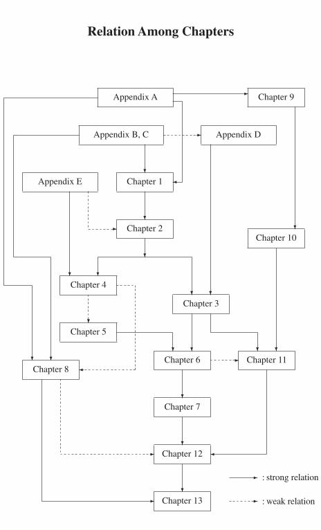
Relation Among Chapters
Chapter 13
Chapter 12
Chapter 7
Chapter 6 Chapter 11
Chapter 3
Chapter 5
Chapter 4
Chapter 8
Chapter 2
Chapter 1
Chapter 10
Appendix E
Appendix B, C
Appendix A
Appendix D
Chapter 9
�
�
�
�� � �
�
�
�
�
�
�
�
�
�
�
� �
�
�
�
�
�
�
�
�
�
�
: strong relation
: weak relation
Introduction
The theory of D-modules plays a key role in algebraic analysis. For the purposes ofthis text, by “algebraic analysis,’’ we mean analysis using algebraic methods, suchas ring theory and homological algebra. In addition to the contributions by Frenchmathematicians, J. Bernstein, and others, this area of research has been extensivelydeveloped since the 1960s by Japanese mathematicians, notably in the importantcontributions of M. Sato, T. Kawai, and M. Kashiwara of the Kyoto school.
To this day, there continue to be outstanding results and significant theories com-ing from the Kyoto school, including Sato’s hyperfunctions, microlocal analysis, D-modules and their applications to representation theory and mathematical physics. Inparticular, the theory of regular holonomic D-modules and their solution complexes(e.g., the theory of the Riemann–Hilbert correspondence which gave a sophisticatedanswer to Hilbert’s 21st problem) was a most important and influential result. Indeed,it provided the germ for the theory of perverse sheaves, which was a natural develop-ment from intersection cohomologies. Moreover, M. Saito used this result effectivelyto construct his theory of Hodge modules, which largely extended the scope of Hodgetheory. In representation theory, this result opened totally new perspectives, such asthe resolution of the Kazhdan–Lusztig conjecture.
As stated above, in addition to the strong impact on analysis which was the initialmain motivation, the theory of algebraic analysis, especially that of D-modules,continues to play a central role in various fields of contemporary mathematics. In fact,D-module theory is a source for creating new research areas from which new theoriesemerge. This striking feature of D-module theory has stimulated mathematicians invarious other fields to become interested in the subject.
Our aim is to give a comprehensive introduction to D-modules. Until recently,in order to really learn it, we had to read and become familiar with many articles,which took long time and considerable effort. However, as we mentioned in thepreface, thanks to some textbooks and monographs, the theory has become muchmore accessible nowadays, especially for those who have some basic knowledge ofcomplex analysis or algebraic geometry. Still, to understand and appreciate the realsignificance of the subject on a deep level, it would be better to learn both the theoryand its typical applications.
2 Introduction
In Part I of this book we introduce D-modules principally in the context of present-ing the theory of the Riemann–Hilbert correspondence. Part II is devoted to explain-ing applications to representation theory, especially to the solution to the Kazhdan–Lusztig conjecture. Since we mainly treat the theory of algebraic D-modules onsmooth algebraic varieties rather than the (original) analytic theory on complex man-ifolds, we shall follow the unpublished notes [Ber3] of Bernstein (the book [Bor3] isalso written along this line). The topics treated in Part II reveal how useful D-moduletheory is in other branches of mathematics. Among other things, the essential useful-ness of this theory contributed heavily to resolving the Kazhdan–Lusztig conjecture,which was of course a great breakthrough in representation theory.
As we started Part II by giving a brief introduction to some basic notions of Liealgebras and algebraic groups using concrete examples, we expect that researchersin other fields can also read Part II without much difficulty.
Let us give a brief overview of the topics developed in this text. First, we explainhow D-modules are related to systems of linear partial differential equations. Let X
be an open subset of Cn and denote by O the commutative ring of complex analyticfunctions globally defined on X. We denote by D the set of linear partial differentialoperators with coefficients in O. Namely, the set D consists of the operators ofthe form
∞∑i1,i2,...,in
fi1,i2,...,in
(∂
∂x1
)i1(
∂
∂x2
)i2
· · ·(
∂
∂xn
)in
(fi1,i2,...,in ∈ O)
(each sum is a finite sum), where (x1, x2, . . . , xn) is a coordinate system of Cn. Notethat D is a non-commutative ring by the composition of differential operators. Sincethe ring D acts on O by differentiation, O is a left D-module. Now, for P ∈ D, letus consider the differential equation
Pu = 0 (0.0.1)
for an unknown function u. According to Sato, we associate to this equation the leftD-module M = D/DP . In this setting, if we consider the set HomD(M, O) ofD-linear homomorphisms from M to O, we get the isomorphism
HomD(M, O) = HomD(D/DP, O)
� {ϕ ∈ HomD(D, O) | ϕ(P ) = 0}.Hence we see by HomD(D, O) � O (ϕ �→ ϕ(1)) that
HomD(M, O) � {f ∈ O | Pf = 0}(Pf = Pϕ(1) = ϕ(P 1) = ϕ(P ) = 0). In other words, the (additive) groupof the holomorphic solutions to the equation (0.0.1) is naturally isomorphic toHomD(M, O). If we replace O with another function space F admitting a natu-ral action of D (for example, the space of C∞-functions, Schwartz distributions,
Introduction 3
Sato’s hyperfunctions, etc.), then HomD(M, F) is the set of solutions to (0.0.1) inthat function space.
More generally, a system of linear partial differential equations of l-unknownfunctions u1, u2, . . . , ul can be written in the form
l∑j=1
Pij uj = 0 (i = 1, 2, . . . , k) (0.0.2)
by using some Pij ∈ D (1 ≤ i ≤ k, 1 ≤ j ≤ l). In this situation we have also asimilar description of the space of solutions. Indeed if we define a left D-module M
by the exact sequence
Dk ϕ−→ Dl −→ M −→ 0 (0.0.3)
ϕ(Q1, Q2, . . . , Qk) =(
k∑i=1
QiPi1,
k∑i=1
QiPi2, . . . ,
k∑i=1
QiPil
),
then the space of the holomorphic solutions to (0.0.2) is isomorphic to HomD(M, O).Therefore, systems of linear partial differential equations can be identified with theD-modules having some finite presentations like (0.0.3), and the purpose of the the-ory of linear PDEs is to study the solution space HomD(M, O). Since the spaceHomD(M, O) does not depend on the concrete descriptions (0.0.2) and (0.0.3) ofM (it depends only on the D-linear isomorphism class of M), we can study theseanalytical problems through left D-modules admitting finite presentations. In thelanguage of categories, the theory of linear PDEs is nothing but the investigationof the contravariant functor HomD(•, O) from the category M(D) of D-modulesadmitting finite presentations to the category M(C) of C-modules.
In order to develop this basic idea, we need to introduce sheaf theory and homo-logical algebra. First, let us explain why sheaf theory is indispensable. It is sometimesimportant to consider solutions locally, rather than globally on X. For example, inthe case of ordinary differential equations (or more generally, the case of integrablesystems), the space of local solutions is always finite dimensional; however, it mayhappen that the analytic continuations (after turning around a closed path) of a so-lution are different from the original one. This phenomenon is called monodromy.Hence we also have to take into account how local solutions are connected to eachother globally.
Sheaf theory is the most appropriate language for treating such problems. There-fore, sheafifying O, D, let us now consider the sheaf OX of holomorphic functionsand the sheaf DX (of rings) of differential operators with holomorphic coefficients.We also consider sheaves of DX-modules (in what follows, we simply call them DX-modules) instead of D-modules. In this setting, the main objects to be studied areleft DX-modules admitting locally finite presentations (i.e., coherent DX-modules).Sheafifying also the solution space, we get the sheaf HomDX
(M, OX) of the holo-morphic solutions to a DX-module M . It follows that what we should investigate isthe contravariant functor HomDX
(•, OX) from the category Modc(DX) of coherentDX-modules to the category Mod(CX) of (sheaves of) CX-modules.
4 Introduction
Let us next explain the need for homological algebra. Although both Modc(DX)
and Mod(CX) are abelian categories, HomDX(•, OX) is not an exact functor. Indeed,
for a short exact sequence
0 −→ M1 −→ M2 −→ M3 −→ 0 (0.0.4)
in the category Modc(DX) the sequence
0 → HomDX(M3, OX) → HomDX
(M2, OX) → HomDX(M1, OX) (0.0.5)
associated to it is also exact; however, the final arrow HomDX(M2, OX) →
HomDX(M1, OX) is not necessarily surjective. Hence we cannot recover informa-
tion about the solutions of M2 from those of M1, M3. A remedy for this is to consideralso the “higher solutions’’ Exti
DX(M, OX) (i = 0, 1, 2, . . . ) by introducing tech-
niques in homological algebra. We have Ext0DX
(M, OX) = HomDX(M, OX) and
the exact sequence (0.0.5) is naturally extended to the long exact sequence
· · · → ExtiDX
(M3, OX) → ExtiDX
(M2, OX) → ExtiDX
(M1, OX)
→ Exti+1DX
(M3, OX) → Exti+1DX
(M2, OX) → Exti+1DX
(M1, OX) → · · · .
Hence the theory will be developed more smoothly by considering all higher solutionstogether.
Furthermore, in order to apply the methods of homological algebra in full general-ity, it is even more effective to consider the object RHomDX
(M, OX) in the derivedcategory (it is a certain complex of sheaves of CX-modules whose i-th cohomologysheaf is Exti
DX(M, OX)) instead of treating the sheaves Exti
DX(M, OX) separately
for various i’s. Among the many other advantages for introducing the methods of ho-mological algebra, we point out here the fact that the sheaf of a hyperfunction solutioncan be obtained by taking the local cohomology of the complex RHomDX
(M, OX)
of holomorphic solutions. This is quite natural since hyperfunctions are determinedby the boundary values (local cohomologies) of holomorphic functions.
Although we have assumed so far that X is an open subset of Cn, we may re-place it with an arbitrary complex manifold. Moreover, also in the framework ofsmooth algebraic varieties over algebraically closed fields k of characteristic zero,almost all arguments remain valid except when considering the solution complexRHomDX
(•, OX), in which case we need to assume again that k = C and return tothe classical topology (not the Zariski topology) as a complex manifold. In this bookwe shall mainly treat D-modules on smooth algebraic varieties over C; however,in this introduction, we will continue to explain everything on complex manifolds.Hence X denotes a complex manifold in what follows.
There were some tentative approaches to D-modules by D. Quillen, Malgrange,and others in the 1960s; however, the real intensive investigation leading to laterdevelopment was started by Kashiwara in his master thesis [Kas1] (we also notethat this important contribution to D-module theory was also made independently byBernstein [Ber1],[Ber2] around the same period). After this groundbreaking work,in collaboration with Kawai, Kashiwara developed the theory of (regular) holonomic
Introduction 5
D-modules [KK3], which is a main theme in Part I of this book. Let us discuss thissubject.
It is well known that the space of the holomorphic solutions to every ordinarydifferential equation is finite dimensional. However, when X is higher dimensional,the dimensions of the spaces of holomorphic solutions can be infinite. This is because,in such cases, the solution contains parameters given by arbitrary functions unlessthe number of given equations is sufficiently large. Hence our task is to look for asuitable class of DX-modules whose solution spaces are finite dimensional. That is,we want to find a generalization of the notion of ordinary differential equations inhigher-dimensional cases.
For this purpose we consider the characteristic variety Ch(M) for a coherentDX-module M , which is a closed analytic subset of the cotangent bundle T ∗X ofX (we sometimes call this the singular support of M and denote it by SS(M)). Weknow by a fundamental theorem of algebraic analysis due to Sato–Kawai–Kashiwara[SKK] that Ch(M) is an involutive subvariety in T ∗X with respect to the canonicalsymplectic structure of T ∗X. In particular, we have dim Ch(M) ≥ dim X for anycoherent DX-module M = 0.
Now we say that a coherent DX-module M is holonomic (a maximally overde-termined system) if it satisfies the equality dim Ch(M) = dim X. Let us give thedefinition of characteristic varieties only in the simple case of DX-modules
M = DX/I, I = DXP1 + DXP2 + · · · + DXPk
associated to the systems
P1u = P2u = · · · = Pku = 0 (Pi ∈ DX) (0.0.6)
for a single unknown function u. In this case, the characteristic variety Ch(M) ofM is the common zero set of the principal symbols σ(Q) (Q ∈ I ) (recall that forQ ∈ DX its principal symbol σ(Q) is a holomorphic function on T ∗X). In manycases Ch(M) coincides with the common zero set of σ(P1), σ (P2), . . . , σ (Pk), but itsometimes happens to be smaller (we also see from this observation that the abstractDX-module M itself is more essential than its concrete expression (0.0.6)).
To make the solution space as small (finite dimensional) as possible we shouldconsider as many equations as possible. That is, we should take the ideal I ⊂ DX
as large as possible. This corresponds to making the ideal generated by the principalsymbols σ(P ) (P ∈ I ) (in the ring of functions on T ∗X) as large as possible, forwhich we have to take the characteristic variety Ch(M), i.e., the zero set of theσ(P )’s, as small as possible. On the other hand, a non-zero coherent DX-module isholonomic if the dimension of its characteristic variety takes the smallest possiblevalue dim X. This philosophical observation suggests a possible connection betweenthe holonomicity and the finite dimensionality of the solution spaces. Indeed suchconnections were established by Kashiwara as we explain below.
Let us point out here that the introduction of the notion of characteristic varietiesis motivated by the ideas of microlocal analysis. In microlocal analysis, the sheafEX of microdifferential operators is employed instead of the sheaf DX of differential
6 Introduction
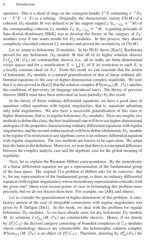
operators. This is a sheaf of rings on the cotangent bundle T ∗X containing π−1DX
(π : T ∗X → X) as a subring. Originally, the characteristic variety Ch(M) of acoherent DX-module M was defined to be the support supp(EX ⊗π−1DX
π−1M) ofthe corresponding coherent EX-module EX ⊗π−1DX
π−1M . A guiding principle ofSato–Kawai–Kashiwara [SKK] was to develop the theory in the category of EX-modules even if one wants results for DX-modules. In this process, they almostcompletely classified coherent EX-modules and proved the involutivity of Ch(M).
Let us return to holonomic D-modules. In his Ph.D. thesis [Kas3], Kashiwaraproved for any holonomic DX-module M that all of its higher solution sheavesExti
DX(M, OX) are constructible sheaves (i.e., all its stalks are finite-dimensional
vector spaces and for a stratification X = ⊔Xi of X its restriction to each Xi is
a locally constant sheaf on Xi). From this result we can conclude that the notionof holonomic DX-module is a natural generalization of that of linear ordinary dif-ferential equations to the case of higher-dimensional complex manifolds. We notethat it is also proved in [Kas3] that the solution complex RHomDX
(M, OX) satisfiesthe conditions of perversity (in language introduced later). The theory of perversesheaves [BBD] must have been motivated (at least partially) by this result.
In the theory of linear ordinary differential equations, we have a good class ofequations called equations with regular singularities, that is, equations admittingonly mild singularities. We also have a successful generalization of this class tohigher dimensions, that is, to regular holonomic DX-modules. There are roughly twomethods to define this class; the first (traditional) one will be to use higher-dimensionalanalogues of the properties characterizing ordinary differential equations with regularsingularities, and the second (rather tactical) will be to define a holonomic DX-moduleto be regular if its restriction to any algebraic curve is an ordinary differential equationwith regular singularities. The two methods are known to be equivalent. We adopthere the latter as the definition. Moreover, we note that there is a conceptual differencebetween the complex analytic case and the algebraic case for the global meaning ofregularity.
Next, let us explain the Riemann–Hilbert correspondence. By the monodromyof a linear differential equation we get a representation of the fundamental groupof the base space. The original 21st problem of Hilbert asks for its converse: thatis, for any representation of the fundamental group, is there an ordinary differentialequation (with regular singularities) whose monodromy representation coincides withthe given one? (there exist several points of view in formulating this problem moreprecisely, but we do not discuss them here. For example, see [AB], and others).
Let us consider the generalization in higher dimensions of this problem. A satis-factory answer in the case of integrable connections with regular singularities wasgiven by P. Deligne [De1]. In this book, we deal with the problem for regularholonomic DX-modules. As we have already seen, for any holonomic DX-moduleM , its solutions Exti
DX(M, OX) are constructible sheaves. Hence, if we denote
by Dbc (CX) the derived category consisting of bounded complexes of CX-modules
whose cohomology sheaves are constructible, the holomorphic solution complexRHomDX
(M, OX) is an object of Dbc (CX). Therefore, denoting by Db
rh(DX) the
Introduction 7
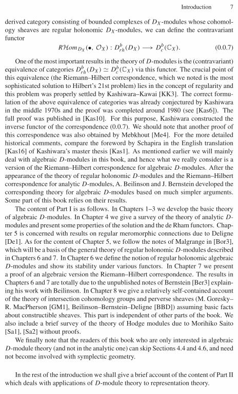
derived category consisting of bounded complexes of DX-modules whose cohomol-ogy sheaves are regular holonomic DX-modules, we can define the contravariantfunctor
RHomDX(•, OX) : Db
rh(DX) −→ Dbc (CX). (0.0.7)
One of the most important results in the theory of D-modules is the (contravariant)equivalence of categories Db
rh(DX) � Dbc (CX) via this functor. The crucial point of
this equivalence (the Riemann–Hilbert correspondence, which we noted is the mostsophisticated solution to Hilbert’s 21st problem) lies in the concept of regularity andthis problem was properly settled by Kashiwara–Kawai [KK3]. The correct formu-lation of the above equivalence of categories was already conjectured by Kashiwarain the middle 1970s and the proof was completed around 1980 (see [Kas6]). Thefull proof was published in [Kas10]. For this purpose, Kashiwara constructed theinverse functor of the correspondence (0.0.7). We should note that another proof ofthis correspondence was also obtained by Mebkhout [Me4]. For the more detailedhistorical comments, compare the foreword by Schapira in the English translation[Kas16] of Kashiwara’s master thesis [Kas1]. As mentioned earlier we will mainlydeal with algebraic D-modules in this book, and hence what we really consider is aversion of the Riemann–Hilbert correspondence for algebraic D-modules. After theappearance of the theory of regular holonomic D-modules and the Riemann–Hilbertcorrespondence for analytic D-modules, A. Beilinson and J. Bernstein developed thecorresponding theory for algebraic D-modules based on much simpler arguments.Some part of this book relies on their results.
The content of Part I is as follows. In Chapters 1–3 we develop the basic theoryof algebraic D-modules. In Chapter 4 we give a survey of the theory of analytic D-modules and present some properties of the solution and the de Rham functors. Chap-ter 5 is concerned with results on regular meromorphic connections due to Deligne[De1]. As for the content of Chapter 5, we follow the notes of Malgrange in [Bor3],which will be a basis of the general theory of regular holonomic D-modules describedin Chapters 6 and 7. In Chapter 6 we define the notion of regular holonomic algebraicD-modules and show its stability under various functors. In Chapter 7 we presenta proof of an algebraic version the Riemann–Hilbert correspondence. The results inChapters 6 and 7 are totally due to the unpublished notes of Bernstein [Ber3] explain-ing his work with Beilinson. In Chapter 8 we give a relatively self-contained accountof the theory of intersection cohomology groups and perverse sheaves (M. Goresky–R. MacPherson [GM1], Beilinson–Bernstein–Deligne [BBD]) assuming basic factsabout constructible sheaves. This part is independent of other parts of the book. Wealso include a brief survey of the theory of Hodge modules due to Morihiko Saito[Sa1], [Sa2] without proofs.
We finally note that the readers of this book who are only interested in algebraicD-module theory (and not in the analytic one) can skip Sections 4.4 and 4.6, and neednot become involved with symplectic geometry.
In the rest of the introduction we shall give a brief account of the content of Part IIwhich deals with applications of D-module theory to representation theory.
8 Introduction
The history of Lie groups and Lie algebras dates back to the 19th century, theperiod of S. Lie and F. Klein. Fundamental results about semisimple Lie groupssuch as those concerning structure theorems, classification, and finite-dimensionalrepresentation theory were obtained by W. Killing, E. Cartan, H. Weyl, and othersuntil the 1930s. Afterwards, the theory of infinite-dimensional (unitary) representa-tions was initiated during the period of World War II by E. P. Wigner, V. Bargmann,I. M. Gelfand, M. A. Naimark, and others, and partly motivated by problems inphysics. Since then and until today the subject has been intensively investigatedfrom various points of view. Besides functional analysis, which was the main methodat the first stage, various theories from differential equations, differential geometry,algebraic geometry, algebraic analysis, etc. were applied to the theory of infinite-dimensional representations. The theory of automorphic forms also exerted a signifi-cant influence. Nowadays infinite-dimensional representation theory is a place wheremany branches of mathematics come together. As contributors representing the de-velopment until the 1970s, we mention the names of Harish-Chandra, B. Kostant,R. P. Langlands.
On the other hand, the theory of algebraic groups was started by the fundamentalworks of C. Chevalley, A. Borel, and others [Ch] and became recognized widelyby the textbook of Borel [Bor1]. Algebraic groups are obtained by replacing theunderlying complex or real manifolds of Lie groups with algebraic varieties. Overthe fields of complex or real numbers algebraic groups form only a special class of Liegroups; however, various new classes of groups are produced by taking other fieldsas the base field. In this book we will only be concerned with semisimple groups overthe field of complex numbers, for which Lie groups and algebraic groups provide thesame class of groups. We regard them as algebraic groups since we basically employthe language of algebraic geometry.
The application of algebraic analysis to representation theory was started by theresolution of the Helgason conjecture [six] due to Kashiwara, A. Kowata, K. Mine-mura, K. Okamoto, T. Oshima, and M. Tanaka. In this book, we focus however onthe resolution of the Kazhdan–Lusztig conjecture which was the first achievement inrepresentation theory obtained by applying D-module theory.
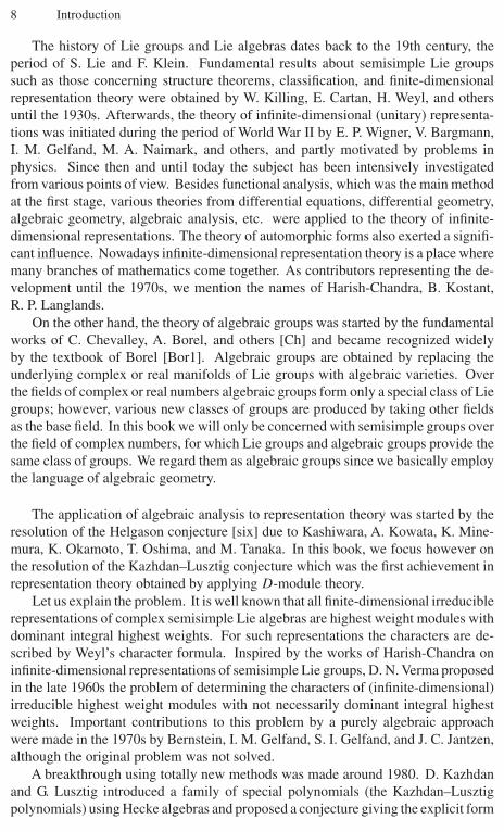
Let us explain the problem. It is well known that all finite-dimensional irreduciblerepresentations of complex semisimple Lie algebras are highest weight modules withdominant integral highest weights. For such representations the characters are de-scribed by Weyl’s character formula. Inspired by the works of Harish-Chandra oninfinite-dimensional representations of semisimple Lie groups, D. N. Verma proposedin the late 1960s the problem of determining the characters of (infinite-dimensional)irreducible highest weight modules with not necessarily dominant integral highestweights. Important contributions to this problem by a purely algebraic approachwere made in the 1970s by Bernstein, I. M. Gelfand, S. I. Gelfand, and J. C. Jantzen,although the original problem was not solved.
A breakthrough using totally new methods was made around 1980. D. Kazhdanand G. Lusztig introduced a family of special polynomials (the Kazhdan–Lusztigpolynomials) using Hecke algebras and proposed a conjecture giving the explicit form
Introduction 9
of the characters of irreducible highest weight modules in terms of these polynomials[KL1]. They also gave a geometric meaning for Kazhdan–Lusztig polynomials usingthe intersection cohomology groups of Schubert varieties. Promptly responding tothis, Beilinson–Bernstein [BB] and J.-L. Brylinski–Kashiwara independently solvedthe conjecture by establishing a correspondence between highest weight modules andthe intersection cohomology complexes of Schubert varieties via D-modules on theflag manifold. This successful achievement, i.e., employing theories and methods,from other fields, was quite astonishing for the specialists who had been studyingthe problem using purely algebraic means. Since then D-module theory has broughtnumerous new developments in representation theory.
Let us explain more precisely the methods used to solve the Kazhdan–Lusztigconjecture. Let G be an algebraic group (or a Lie group), g its Lie algebra and U(g)
the universal enveloping algebra of g. If X is a smooth G-variety and V is a G-equivariant vector bundle on X, the set �(X, V) of global sections of V naturally hasa g-module structure. The construction of the representation of g (or of G) in thismanner is a fundamental technique in representation theory.
Let us now try to generalize this construction. Denote by DVX ⊂ EndC(V)
the sheaf of rings of differential operators acting on the sections of V . Then DVX is
isomorphic to V ⊗OXDX ⊗OX
V∗ which coincides with the usual DX when V = OX.In terms of DV
X the g-module structure on �(X, V) can be described as follows. Notethat we have a canonical ring homomorphism U(g) → �(X, DV
X) induced by theG-action on V . Since V is a DV
X -module, �(X, V) is a �(X, DVX)-module, and
hence a g-module through the ring homomorphism U(g) → �(X, DVX). From this
observation, we see that we can replace V with other DVX -modules. That is, for any
DVX -module M the C-vector space �(X, M) is endowed with a g-module structure.
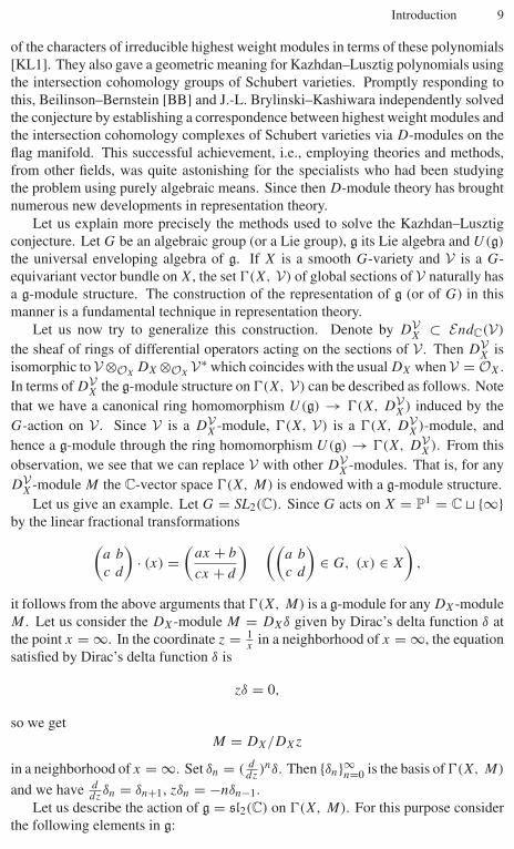
Let us give an example. Let G = SL2(C). Since G acts on X = P1 = C � {∞}by the linear fractional transformations(
a b
c d
)· (x) =
(ax + b
cx + d
) ((a b
c d
)∈ G, (x) ∈ X
),
it follows from the above arguments that �(X, M) is a g-module for any DX-moduleM . Let us consider the DX-module M = DXδ given by Dirac’s delta function δ atthe point x = ∞. In the coordinate z = 1
xin a neighborhood of x = ∞, the equation
satisfied by Dirac’s delta function δ is
zδ = 0,
so we getM = DX/DXz
in a neighborhood of x = ∞. Set δn = ( ddz
)nδ. Then {δn}∞n=0 is the basis of �(X, M)
and we have ddz
δn = δn+1, zδn = −nδn−1.Let us describe the action of g = sl2(C) on �(X, M). For this purpose consider
the following elements in g:
10 Introduction
h =(
1 00 −1
), e =
(0 10 0
), f =
(0 01 0
)(these elements h, e, f form a basis of g). Then the ring homomorphism U(g) →�(X, DX) is given by
h �−→ 2zd
dz, e �−→ z2 d
dz, f �−→ − d
dz.
For example, since
exp(−te) ·(
1
z
)=(
1
z/(1 − tz)
),
for ϕ(z) ∈ OX we get
(e · ϕ)(z) = d
dtϕ
(z
1 − tz
)∣∣∣∣t=0
=(
z2 d
dzϕ
)(z)
and e �→ z2 ddz
. Therefore we obtain
h · δn = −2(n + 1)δn, e · δn = n(n + 1)δn−1, f · δn = −δn+1,
from which we see that �(X, M) is the infinite-dimensional irreducible highest weightmodule with highest weight −2.
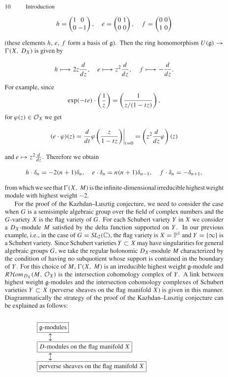
For the proof of the Kazhdan–Lusztig conjecture, we need to consider the casewhen G is a semisimple algebraic group over the field of complex numbers and theG-variety X is the flag variety of G. For each Schubert variety Y in X we considera DX-module M satisfied by the delta function supported on Y . In our previousexample, i.e., in the case of G = SL2(C), the flag variety is X = P1 and Y = {∞} isa Schubert variety. Since Schubert varieties Y ⊂ X may have singularities for generalalgebraic groups G, we take the regular holonomic DX-module M characterized bythe condition of having no subquotient whose support is contained in the boundaryof Y . For this choice of M , �(X, M) is an irreducible highest weight g-module andRHomDX
(M, OX) is the intersection cohomology complex of Y . A link betweenhighest weight g-modules and the intersection cohomology complexes of Schubertvarieties Y ⊂ X (perverse sheaves on the flag manifold X) is given in this manner.Diagrammatically the strategy of the proof of the Kazhdan–Lusztig conjecture canbe explained as follows:
g-modules�D-modules on the flag manifold X�perverse sheaves on the flag manifold X

Introduction 11
Here the first arrow is what we have briefly explained above, and the secondone is the Riemann–Hilbert correspondence, a general theory of D-modules. Thefirst arrow is called the Beilinson–Bernstein correspondence, which asserts that thecategory of U(g)-modules with the trivial central character and that of DX-modulesare equivalent. By this correspondence, for a DX-module M on the flag manifold X,we associate to it the U(g)-module �(X, M). As a result, we can translate variousproblems for g-modules into those for regular holonomic D-modules (or through theRiemann–Hilbert correspondence, those for constructible sheaves).
The content of Part II is as follows. We review some preliminary results onalgebraic groups in Chapters 9 and 10. In Chapters 11 and 12 we will explain howthe Kazhdan–Lusztig conjecture was solved. Finally, in Chapter 13, a realizationof Hecke algebras will be given by the theory of Hodge modules, and the relationbetween the intersection cohomology groups of Schubert varieties and Hecke algebraswill be explained.
Let us briefly mention some developments of the theory, which could not be treatedin this book. We can also formulate conjectures, similar to the Kazhdan–Lusztigconjecture, for Kac–Moody Lie algebras, i.e., natural generalizations of semisimpleLie algebras. In this case, we have to study two cases separately: (a) the case whenthe highest weight is conjugate to a dominant weight by the Weyl group, (b) thecase when the highest weight is conjugate to an anti-dominant weight by the Weylgroup. Moreover, Lusztig proposed certain Kazhdan–Lusztig type conjectures alsofor the following objects: (c) the representations of reductive algebraic groups inpositive characteristics, (d) the representations of quantum groups in the case whenthe parameter q is a root of unity. The conjecture of the case (a) was solved byKashiwara (and Tanisaki) [Kas15], [KT2] and L. Casian [Ca1]. Following the so-called Lusztig program, the other conjectures were also solved:
(A) the equivalence of (c) and (d): H. H. Andersen, J. C. Jantzen, W. Soergel [AJS].(B) the equivalence of (b) and (d) for affine Lie algebras: Kazhdan–Lusztig [KL3].(C) the proof of (b) for affine Lie algebras: Kashiwara–Tanisaki [KT3] and Casian
[Ca2].
Part I
D-Modules and Perverse Sheaves
1
Preliminary Notions
In this chapter we introduce several standard operations for D-modules and presentsome fundamental results concerning them such as Kashiwara’s equivalence theorem.
1.1 Differential operators
Let X be a smooth (non-singular) algebraic variety over the complex number field Cand OX the sheaf of rings of regular functions (structure sheaf) on it. We denote by�X the sheaf of vector fields (tangent sheaf, see Appendix A) on X:
�X = DerCX(OX)
= {θ ∈ EndCX(OX) | θ(fg) = θ(f )g + f θ(g) (f, g ∈ OX)}.
Hereafter, if there is no risk of confusion, we use the notation f ∈ OX for a localsection f of OX. Since X is smooth, the sheaf �X is locally free of rank n = dim X
over OX. We will identify OX with a subsheaf of EndCX(OX) by identifying f ∈ OX
with [OX g �→ fg ∈ OX] ∈ EndCX(OX). We define a sheaf DX as the C-
subalgebra of EndCX(OX) generated by OX and �X. We call this sheaf DX the
sheaf of differential operators on X. For any point of X we can take its affine openneighborhood U and a local coordinate system {xi, ∂i}1≤i≤n on it satisfying
xi ∈ OX(U), �U =n⊕
i=1
OU ∂i, [∂i, ∂j ] = 0, [∂i, xj ] = δij
(see Appendix A). Hence we have
DU = DX|U =⊕α∈Nn
OU ∂αx (∂α
x := ∂α11 ∂
α22 · · · ∂αn
n ).
Here, N denotes the set of non-negative integers.

16 1 Preliminary Notions
Exercise 1.1.1. Let U be an affine open subset of X. Show that DX(U) is naturallyisomorphic to the C-algebra generated by elements {f , θ | f ∈ OX(U), θ ∈ �X(U)}satisfying the following fundamental relations:
(1) f1 + f2 = f1 + f2, f1f2 = f1f2 (f1, f2 ∈ OX(U)),
(2) θ1 + θ2 = θ1 + θ2, [θ1, θ2] = ˜[θ1, θ2] (θ1, θ2 ∈ �X(U)),
(3) f θ = f θ (f ∈ OX(U), θ ∈ �X(U)),
(4) [θ , f ] = θ (f ) (f ∈ OX(U), θ ∈ �X(U)).
Exercise 1.1.2. Let {xi, ∂i}1≤i≤n be a local coordinate system on an affine open subsetU of X. For P = ∑
α∈Nn aα(x)∂αx ∈ DX(U) we define its total symbol σ(P )(x, ξ)
by σ(P )(x, ξ) := ∑α∈Nn aα(x)ξα (ξα := ξ
α11 ξ
α22 · · · ξαn
n ). For P , Q ∈ DX(U)
show that the total symbol σ(R)(x, ξ) of the product R = PQ ∈ DX(U) is given by
σ(R)(x, ξ) =∑
α∈Nn
1
α!∂αξ σ (P )(x, ξ) · ∂α
x σ (Q)(x, ξ),
where we set α! = α1!α2! · · · αn! for each α ∈ Nn (this is the “Leibniz rule’’).
Let U be an affine open subset of X with a local coordinate system {xi, ∂i}. Wedefine the order filtration F of DU by
FlDU =∑|α|≤l
OU ∂αx
(l ∈ N, |α| =
∑i
αi
).
More generally, for an arbitrary open subset V of X we can define the order filtrationF of DX over V by
(FlDX)(V )
= {P ∈ DX(V ) | resVU P ∈ FlDX(U) for any affine open subset U of V },
where resVU : DX(V ) → DX(U) is the restriction map (see also Exercise 1.1.4
below). For convenience we set FpDX = 0 for p < 0. The following result isobvious.
Proposition 1.1.3.(i) {Fl}l∈N is an increasing filtration of DX such that DX = ⋃
l∈N FlDX and eachFlDX is a locally free module over OX.
(ii) F0DX = OX, (FlDX)(FmDX) = Fl+mDX.(iii) If P ∈ FlDX and Q ∈ FmDX, then [P, Q] ∈ Fl+m−1DX.
Exercise 1.1.4. Show that the formula
FlDX = {P ∈ EndC(OX) | [P, f ] ∈ Fl−1DX (∀f ∈ OX)} (l ∈ N).
(Note that this recursive expression of FlDX together with DX = ⋃l∈N FlDX gives
an alternative intrinsic definition of DX.)
1.2 D-modules—warming up 17
Principal symbols
For the sheaf (DX, F ) of filtered rings let us consider its graded ring
gr DX = grF DX =∞⊕l=0
grl DX (grl DX = FlDX/Fl−1DX, F−1DX = 0).
Then by Proposition 1.1.3 gr DX is a sheaf of commutative algebras finitely generatedover OX. Take an affine chart U with a coordinate system {xi, ∂i} and set
ξi := ∂i mod F0DU (= OU ) ∈ gr1 DU .
Then we have
grl DU = FlDU /Fl−1DU =⊕|α|=l
OU ξα,
gr DU = OU [ξ1, ξ2, . . . , ξn].For a differential operator P ∈ FlDU \ Fl−1DU the corresponding section σl(P ) ∈grl DU ⊂ OU [ξ1, ξ2, . . . , ξn] is called the principal symbol of P .
We can globalize this notion as follows. Let T ∗X be the cotangent bundle ofX and let π : T ∗X → X be the projection. We may regard ξ1, . . . , ξn as thecoordinate system of the cotangent space
⊕ni=1 Cdxi , and hence OU [ξ1, . . . , ξn]
is canonically identified with the sheaf π∗OT ∗X|U of algebras. Thus we obtain acanonical identification
gr DX � π∗OT ∗X(� Symm �X).
Therefore, for P ∈ FlDX we can associate to it a regular function σl(P ) globallydefined on the cotangent bundle T ∗X.
1.2 D-modules—warming up
As we have already explained in the introduction, a system of differential equationscan be regarded as a “coherent’’ left D-module.
Let X be a smooth algebraic variety. We say that a sheaf M on X is a left DX-module if M(U) is endowed with a left DX(U)-module structure for each open subsetU of X and these actions are compatible with restriction morphisms.
Note that OX is a left DX-module via the canonical action of DX.We have the following very easy (but useful) interpretation of the notion of left
DX-modules.
Lemma 1.2.1. Let M be an OX-module. Giving a left DX-module structure on M
extending the OX-module structure is equivalent to giving a C-linear morphism
∇ : �X → EndC(M) (θ �→ ∇θ ),
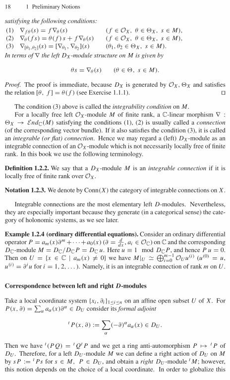
18 1 Preliminary Notions
satisfying the following conditions:
(1) ∇f θ (s) = f ∇θ (s) (f ∈ OX, θ ∈ �X, s ∈ M),
(2) ∇θ (f s) = θ(f ) s + f ∇θ (s) (f ∈ OX, θ ∈ �X, s ∈ M),
(3) ∇[θ1,θ2](s) = [∇θ1 , ∇θ2 ](s) (θ1, θ2 ∈ �X, s ∈ M).
In terms of ∇ the left DX-module structure on M is given by
θs = ∇θ (s) (θ ∈ �, s ∈ M).
Proof. The proof is immediate, because DX is generated by OX, �X and satisfiesthe relation [θ, f ] = θ(f ) (see Exercise 1.1.1). ��
The condition (3) above is called the integrability condition on M .For a locally free left OX-module M of finite rank, a C-linear morphism ∇ :
�X → EndC(M) satisfying the conditions (1), (2) is usually called a connection(of the corresponding vector bundle). If it also satisfies the condition (3), it is calledan integrable (or flat) connection. Hence we may regard a (left) DX-module as anintegrable connection of an OX-module which is not necessarily locally free of finiterank. In this book we use the following terminology.
Definition 1.2.2. We say that a DX-module M is an integrable connection if it islocally free of finite rank over OX.
Notation 1.2.3. We denote by Conn(X) the category of integrable connections on X.
Integrable connections are the most elementary left D-modules. Nevertheless,they are especially important because they generate (in a categorical sense) the cate-gory of holonomic systems, as we see later.
Example 1.2.4 (ordinary differential equations). Consider an ordinary differentialoperator P = am(x)∂m +· · ·+a0(x) (∂ = d
dx, ai ∈ OC) on C and the corresponding
DC-module M = DC/DCP = DC u. Here u ≡ 1 mod DCP , and hence P u = 0.Then on U = {x ∈ C | am(x) = 0} we have M|U � ⊕m−1
i=0 OU u(i) (u(0) = u,u(i) = ∂iu for i = 1, 2, . . . ). Namely, it is an integrable connection of rank m on U .
Correspondence between left and right D-modules
Take a local coordinate system {xi, ∂i}1≤i≤n on an affine open subset U of X. ForP (x, ∂) = ∑
α aα(x)∂α ∈ DU consider its formal adjoint
tP (x, ∂) :=∑
α
(−∂)αaα(x) ∈ DU .
Then we have t (PQ) = tQtP and we get a ring anti-automorphism P �→ tP ofDU . Therefore, for a left DU -module M we can define a right action of DU on M
by sP := tP s for s ∈ M, P ∈ DU , and obtain a right DU -module tM; however,this notion depends on the choice of a local coordinate. In order to globalize this
1.2 D-modules—warming up 19
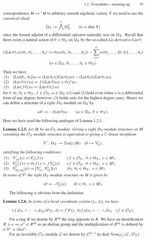
correspondence M ↔ tM to arbitrary smooth algebraic variety X we need to use thecanonical sheaf
�X :=n∧
�1X (n = dim X)
since the formal adjoint of a differential operator naturally acts on �X. Recall thatthere exists a natural action of θ ∈ �X on �X by the so-called Lie derivative Lie θ :
((Lie θ) ω)(θ1, θ2, . . . , θn) := θ(ω(θ1, θ2, . . . , θn)) −n∑
i=1
ω(θ1, . . . , [θ, θi], . . . , θn)
(ω ∈ �X, θ1, . . . , θn ∈ �X).
Then we have(1) (Lie[θ1, θ2])ω = (Lie θ1)((Lie θ2)ω) − (Lie θ2)((Lie θ1)ω),
(2) (Lie θ)(f ω) = f ((Lie θ)ω) + θ(f )ω,
(3) (Lie(f θ))ω = (Lie θ)(f ω)
for θ, θ1, θ2 ∈ �X, f ∈ OX, ω ∈ �X ((1) and (2) hold even when ω is a differentialform of any degree; however, (3) holds only for the highest degree case). Hence wecan define a structure of a right DX-module on �X by
ωθ := −(Lie θ)ω (ω ∈ �X, θ ∈ �X).
Here we have used the following analogue of Lemma 1.2.1.
Lemma 1.2.5. Let M be an OX-module. Giving a right DX-module structure on M
extending the OX-module structure is equivalent to giving a C-linear morphism
∇′ : �X → EndC(M) (θ �→ ∇′θ ),
satisfying the following conditions:
(1) ∇′f θ (s) = ∇′
θ (f s) (f ∈ OX, θ ∈ �X, s ∈ M),
(2) ∇′θ (f s) = θ(f ) s + f ∇′
θ (s) (f ∈ OX, θ ∈ �X, s ∈ M),
(3) ∇′[θ1,θ2](s) = [∇′θ1
, ∇′θ2
](s) (θ1, θ2 ∈ �X, s ∈ M).
In terms of ∇′ the right DX-module structure on M is given by
sθ = −∇′θ (s) (θ ∈ �, s ∈ M).
The following is obvious from the definition.
Lemma 1.2.6. In terms of a local coordinate system {xi, ∂i}, we have
(f dx1 ∧ · · · ∧ dxn)P (x, ∂) = (tP (x, ∂)f )dx1 ∧ · · · ∧ dxn (f ∈ OX).
For a ring R we denote by Rop the ring opposite to R. We have an identificationR a ↔ a◦ ∈ Rop as an abelian group and the multiplication of Rop is defined bya◦b◦ = (ba)◦.
For an invertible OX-module L we denote by L⊗−1 its dual HomOX(L, OX).

20 1 Preliminary Notions
The right DX-module structure on �X gives a homomorphism DopX → EndC(�X)
of C-algebras. Note that we have an isomorphism
EndC(�X) � �X ⊗OXEndC(OX) ⊗OX
�⊗−1X
of sheaves of rings, where the left and the rightOX-module structure onEndC(OX) aregiven by the left- and right-multiplication of OX (regarded as a subring of EndC(OX))inside the (non-commutative) ring EndC(OX), and the above isomorphism is given byassociating ω⊗F ⊗η ∈ �X ⊗OX
EndC(OX)⊗OX�⊗−1
X (ω ∈ �X, F ∈ EndC(OX),η ∈ �⊗−1
X ) to the section of EndC(�X) given by ω′ �→ F(〈η, ω′〉)ω. By Lemma 1.2.6(or by Exercise 1.1.4) we have the following.
Lemma 1.2.7. We have a canonical isomorphism
DopX � �X ⊗OX
DX ⊗OX�⊗−1
X
of C-algebras.
In terms of a local coordinate {xi, ∂i} the correspondence in Lemma 1.2.7 isgiven by associating P ◦ ∈ D
opX (P ∈ DX) to dx ⊗ tP ⊗ dx⊗−1, where dx =
dx1 ∧ · · · ∧ dxn ∈ �X and dx⊗−1 ∈ �⊗−1X is given by 〈dx, dx⊗−1〉 = 1.
Notation 1.2.8. For a ring (or a sheaf of rings on a topological space) R we denoteby Mod(R) the abelian category of left R-modules.
We will identify Mod(Rop) with the category of right R-modules. We easily seefrom Lemmas 1.2.1 and 1.2.5 the following.
Proposition 1.2.9. Let M, N ∈ Mod(DX) and M ′, N ′ ∈ Mod(DopX ). Then we have
(i) M ⊗OXN ∈ Mod(DX) ; θ(s ⊗ t) = θ(s) ⊗ t + s ⊗ θ(t),
(ii) M ′ ⊗OXN ∈ Mod(D
opX ) ; (s′ ⊗ t)θ = s′θ ⊗ t − s′ ⊗ θt,
(iii) HomOX(M, N) ∈ Mod(DX) ; (θψ)(s) = θ(ψ(s)) − ψ(θ(s)),
(iv) HomOX(M ′, N ′) ∈ Mod(DX) ; (θψ)(s) = −ψ(s)θ + ψ(sθ),
(v) HomOX(M, N ′) ∈ Mod(D
opX ) ; (ψθ)(s) = ψ(s)θ + ψ(θ(s)).
Here θ ∈ �X.
Remark 1.2.10. Let X be a smooth algebraic curve X of genus g. Note that deg OX =0 and deg �X = 2g − 2. More generally, it is known that an invertible OX-moduleL is equipped with a left (resp. right) DX-module structure if and only if deg L = 0(resp. 2g − 2). This gives an easy way to memorize all of the consequences ofProposition 1.2.9 (Oda’s rule [O]). It also explains the reason why M ′ ⊗OX
N ′ forM ′, N ′ ∈ Mod(D
opX ) is excluded from Proposition 1.2.9. Even if we do not know
that deg �X = 2g − 2, we can get the right answer by using the correspondences“left’’ ↔ 0, “right’’ ↔ 1 and ⊗ ↔ +, Hom(•, �) = −• + �.
By Proposition 1.2.9 we easily see the following results.
1.3 Inverse and direct images I 21
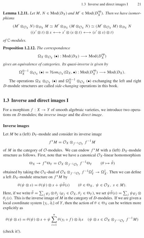
Lemma 1.2.11. Let M, N ∈ Mod(DX) and M ′ ∈ Mod(DopX ). Then we have isomor-
phisms
(M ′ ⊗OXN) ⊗DX
M � M ′ ⊗DX(M ⊗OX
N) � (M ′ ⊗OXM) ⊗DX
N
((s′ ⊗ t) ⊗ s ←→ s′ ⊗ (s ⊗ t) ←→ (s′ ⊗ s) ⊗ t)
of C-modules.
Proposition 1.2.12. The correspondence
�X ⊗OX(•) : Mod(DX) −→ Mod(D
opX )
gives an equivalence of categories. Its quasi-inverse is given by
�⊗−1X ⊗OX
(•) = HomOX(�X, •) : Mod(D
opX ) −→ Mod(DX).
The operations �X ⊗OX(•) and �⊗−1
X ⊗OX(•) exchanging the left and right
D-module structures are called side-changing operations in this book.
1.3 Inverse and direct images I
For a morphism f : X → Y of smooth algebraic varieties, we introduce two opera-tions on D-modules; the inverse image and the direct image.
Inverse images
Let M be a (left) DY -module and consider its inverse image
f ∗M = OX ⊗f −1OYf −1M
of M in the category of O-modules. We can endow f ∗M with a (left) DX-modulestructure as follows. First, note that we have a canonical OX-linear homomorphism
�X → f ∗�Y = OX ⊗f −1OYf −1�Y (θ �→ θ )
obtained by taking the OX-dual of OX ⊗f −1OYf −1�1
Y → �1X. Then we can define
a left DX-module structure on f ∗M by
θ(ψ ⊗ s) = θ(ψ) ⊗ s + ψθ(s) (θ ∈ �X, ψ ∈ OX, s ∈ M).
Here, if we write θ = ∑j ϕj ⊗ θj (ϕj ∈ OX, θj ∈ �Y ), we set ψθ(s) = ∑
j ψϕj ⊗θj (s). This is the inverse image of M in the category of D-modules. If we are given alocal coordinate system {yi, ∂i} of Y , then the action of θ ∈ �X can be written moreexplicitly as
θ(ψ ⊗ s) = θ(ψ) ⊗ s + ψ
n∑i=1
θ(yi ◦ f ) ⊗ ∂is (ψ ⊗ s ∈ OX ⊗f −1OYf −1M)
(check it!).
22 1 Preliminary Notions
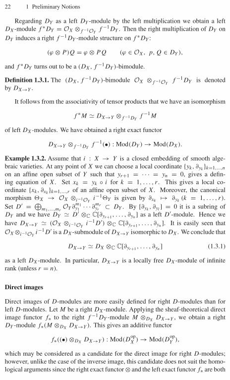
Regarding DY as a left DY -module by the left multiplication we obtain a leftDX-module f ∗DY = OX ⊗f −1OY
f −1DY . Then the right multiplication of DY onDY induces a right f −1DY -module structure on f ∗DY :
(ϕ ⊗ P)Q = ϕ ⊗ PQ (ϕ ∈ OX, p, Q ∈ DY ),
and f ∗DY turns out to be a (DX, f −1DY )-bimodule.
Definition 1.3.1. The (DX, f −1DY )-bimodule OX ⊗f −1OYf −1DY is denoted
by DX→Y .
It follows from the associativity of tensor products that we have an isomorphism
f ∗M � DX→Y ⊗f −1DYf −1M
of left DX-modules. We have obtained a right exact functor
DX→Y ⊗f −1DYf −1(•) : Mod(DY ) → Mod(DX).
Example 1.3.2. Assume that i : X → Y is a closed embedding of smooth alge-braic varieties. At any point of X we can choose a local coordinate {yk, ∂yk
}k=1,...,n
on an affine open subset of Y such that yr+1 = · · · = yn = 0, gives a defin-ing equation of X. Set xk = yk ◦ i for k = 1, . . . , r . This gives a local co-ordinate {xk, ∂xk
}k=1,...,r of an affine open subset of X. Moreover, the canonicalmorphism �X → OX ⊗i−1OY
i−1�Y is given by ∂xk�→ ∂yk
(k = 1, . . . , r).Set D′ = ⊕
m1,...,mrOY ∂
m1y1 · · · ∂mr
yr⊂ DY . By [∂yk
, ∂yl] = 0 it is a subring of
DY and we have DY � D′ ⊗C C[∂yr+1 , . . . , ∂yn ] as a left D′-module. Hence wehave DX→Y � (OX ⊗i−1OY
i−1D′) ⊗C C[∂yr+1 , . . . , ∂yn ]. It is easily seen thatOX ⊗i−1OY
i−1D′ is a DX-submodule of DX→Y isomorphic to DX. We conclude that
DX→Y � DX ⊗C C[∂yr+1 , . . . , ∂yn ] (1.3.1)
as a left DX-module. In particular, DX→Y is a locally free DX-module of infiniterank (unless r = n).
Direct images
Direct images of D-modules are more easily defined for right D-modules than forleft D-modules. Let M be a right DX-module. Applying the sheaf-theoretical directimage functor f∗ to the right f −1DY -module M ⊗DX
DX→Y , we obtain a rightDY -module f∗(M ⊗DX
DX→Y ). This gives an additive functor
f∗((•) ⊗DXDX→Y ) : Mod(D
opX ) → Mod(D
opY ),
which may be considered as a candidate for the direct image for right D-modules;however, unlike the case of the inverse image, this candidate does not suit the homo-logical arguments since the right exact functor ⊗ and the left exact functor f∗ are both
1.3 Inverse and direct images I 23
involved. The right definition in the language of derived categories will be given later.Here we consider how to construct direct images for left D-modules. They can be de-fined by the correspondence (side-changing) of left and right D-modules explained inProposition 1.2.12. Namely, a candidate for the direct image Mod(DX) → Mod(DY )
is obtained by the commutativity of
Mod(DX) −−−−→ Mod(DY )
�X⊗OX(•)
⏐⏐� �⏐⏐�Y ⊗OY
(•)
Mod(DopX ) −−−−→ Mod(D
opY )
where the lower horizontal arrow is given by f∗((•) ⊗DXDX→Y ). Thus, to a a left
DX-module M we can associate a left DY -module
�⊗−1Y ⊗OY
f∗((�X ⊗OXM) ⊗DX
DX→Y ).
By Lemma 1.2.11 we have an isomorphism
(�X ⊗OXM) ⊗DX
DX→Y � (�X ⊗OXDX→Y ) ⊗DX
M
of right f −1DY -modules, where f −1DY acts on (�X ⊗OXDX→Y ) ⊗DX
M by
((ω ⊗ R) ⊗ s)P = (ω ⊗ RP) ⊗ s (ω ∈ �X, R ∈ DX→Y , s ∈ M, P ∈ DY ).
Hence we have
�⊗−1Y ⊗OY
f∗((�X ⊗OXM) ⊗DX
DX→Y )
� �⊗−1Y ⊗OY
f∗((�X ⊗OXDX→Y ) ⊗DX
M)
� f∗((�X ⊗OXDX→Y ⊗f −1OY
f −1�⊗−1Y ) ⊗DX
M).
Definition 1.3.3. We define a (f −1DY , DX)-bimodule DY←X by
DY←X := �X ⊗OXDX→Y ⊗f −1OY
f −1�⊗−1Y .
We call DX→Y and DY←X the transfer bimodules for f : X → Y .In terms of DY←X our tentative definition of the direct image for left D-modules
is given byf∗(DY←X ⊗DX
(•)) : Mod(DX) → Mod(DY ).
By DopY � �Y ⊗OY
DY ⊗OY�⊗−1
Y we have
DY←X = �X ⊗OX(OX ⊗f −1OY
f −1DY ) ⊗f −1OYf −1�⊗−1
Y ,
= �X ⊗f −1OYf −1(DY ⊗OY
�⊗−1Y ),
� �X ⊗f −1OYf −1(�⊗−1
Y ⊗OYD
opY )
� f −1(DY ⊗OY�⊗−1
Y ) ⊗f −1OY�X,
where the last isomorphism is given by
ω ⊗ η ⊗ P ◦ ↔ P ⊗ η ⊗ ω (ω ∈ �X, η ∈ �⊗−1Y , P ∈ DY ).
Hence we obtain the following different description of DY←X.

24 1 Preliminary Notions
Lemma 1.3.4. As a (f −1DY , DX)-bimodule we have
DY←X � f −1(DY ⊗OY�⊗−1
Y ) ⊗f −1OY�X.
Here the right-hand side is endowed with a left f −1DY -module structure inducedfrom the left multiplication of DY on DY . The right DX-module structure on it isgiven as follows. The right multiplication of DY on DY gives a right DY -modulesstructure on DY . By the side-changing operation, DY ⊗OY
�⊗−1Y is a left DY -mod-
ule. Applying the inverse image functor for left D-modules we get a left DX-modulef −1(DY ⊗OY
�⊗−1Y )⊗f −1OY
OX. Finally, by the side-changing operation we obtaina right DX-module
f −1(DY ⊗OY�⊗−1
Y ) ⊗f −1OYOX ⊗OX
�X = f −1(DY ⊗OY�⊗−1
Y ) ⊗f −1OY�X.
Example 1.3.5. We give a local description of DY←X for a closed embeddingi : X → Y of smooth algebraic varieties. Take a local coordinate {yk, ∂yk
}1≤k≤n
of Y as in Example 1.3.2, and set xk = yk ◦ i for k = 1, . . . , r . Note that
DY←X = (i−1DY ⊗i−1OYOX) ⊗OX
(i−1�⊗−1Y ⊗i−1OY
�X).
We (locally) identify i−1�⊗−1Y ⊗i−1OY
�X with OX via the section
(dy1 ∧ · · · ∧ dyn)⊗−1 ⊗ (dx1 ∧ · · · ∧ dxr).
Set D′ = ⊕m1,...,mr
∂m1y1 · · · ∂mr
yrOY ⊂ DY . It is a subring of DY and we have
DY � C[∂yr+1 , . . . , ∂yn ] ⊗C D′ as a right D′-module. Hence we have
DY←X � C[∂yr+1 , . . . , ∂yn ] ⊗C (i−1D′ ⊗i−1OYOX). (1.3.2)
The right DX-action on the right-hand side is induced from the right DX-action oni−1D′ ⊗i−1OY
OX given by
(P ⊗ 1)∂xk= (P ∂yk
) ⊗ 1, (P ⊗ 1)ϕ = P ⊗ ϕ = P ϕ ⊗ 1 (P ∈ D′, ϕ ∈ OX),
where ϕ ∈ OY is such that ϕ|X = ϕ. Hence we have i−1D′ ⊗i−1OYOX � DX and
we obtain a local isomorphism
DY←X � C[∂yr+1 , . . . , ∂yn ] ⊗C DX.
The left i−1DY -module structure on the right-hand side can be described asfollows. Note that DY � C[∂yr+1 , . . . , ∂yn ] ⊗C D′. Hence we have i−1DY �C[∂yr+1 , . . . , ∂yn ] ⊗C i−1D′. Therefore, it is sufficient to give the actions ofC[∂yr+1 , . . . , ∂yn ] and i−1D′ on C[∂yr+1 , . . . , ∂yn ] ⊗C DX.
The action of C[∂yr+1 , . . . , ∂yn ] is given by the multiplication on the first factorC[∂yr+1 , . . . , ∂yn ] of the tensor product. Let Q ∈ i−1D′, F ∈ C[∂yr+1 , . . . , ∂yn ] andR ∈ DX. If we have QF = ∑
k FkQk (Fk ∈ C[∂yr+1 , . . . , ∂yn ], Qk ∈ i−1D′) in thering i−1DY , then the action of Q ∈ i−1D′ on F ⊗ R ∈ C[∂yr+1 , . . . , ∂yn ] ⊗C DX
is given by Q(F ⊗ R) = ∑k Fk ⊗ QkR, where the left i−1D′-module structure on
DX � i−1D′ ⊗i−1OYOX is given by
Q(P ⊗ 1) = QP ⊗ 1 (P, Q ∈ D′).

1.4 Some categories of D-modules 25
1.4 Some categories of D-modules
On algebraic varieties, the category of quasi-coherent sheaves (over O) is sufficientlywide and suitable for various algebraic operations (see Appendix A for the notion ofquasi-coherent sheaves). Since our sheaf DX is locally free over OX, it is quasi-coherent over OX. We mainly deal with DX-modules which are quasi-coherentover OX.
Notation 1.4.1. For an algebraic variety X we denote the category of quasi-coherentOX-modules by Modqc(OX). For a smooth algebraic variety X we denote byModqc(DX) the category of OX-quasi-coherent DX-modules.
The category Modqc(DX) is an abelian category.It is well known that for affine algebraic varieties X,
(a) the global section functor �(X, •) : Modqc(OX) → Mod(�(X, OX)) is exact,(b) if �(X, M) = 0 for M ∈ Modqc(OX), then M = 0.
In fact, an algebraic variety is affine if and only if the condition (a) is satisfied.Replacing OX by DX we come to the following notion.
Definition 1.4.2. A smooth algebraic variety X is called D-affine if the followingconditions are satisfied:
(a) the global section functor �(X, •) : Modqc(DX) → Mod(�(X, DX)) is exact,(b) if �(X, M) = 0 for M ∈ Modqc(DX), then M = 0.
The following is obvious.
Proposition 1.4.3. Any smooth affine algebraic variety is D-affine.
As in the case of quasi-coherent O-modules on affine varieties we have the fol-lowing.
Proposition 1.4.4. Assume that X is D-affine.
(i) Any M ∈ Modqc(DX) is generated over DX by its global sections.(ii) The functor
�(X, •) : Modqc(DX) → Mod(�(X, DX))
gives an equivalence of categories.
Proof. (i) For M ∈ Modqc(DX) let M0 be the image of the natural morphism DX ⊗C
�(X, M) → M in M (the submodule of M generated by global sections). Since X
is D-affine, we obtain an exact sequence
0 → �(X, M0)i
→ �(X, M) → �(X, M/M0) → 0.
Since i is an isomorphism by the definition of M0, we have �(X, M/M0) = 0. SinceX is D-affine, we get M/M0 = 0, i.e., M = M0.
26 1 Preliminary Notions
(ii) We will show that the functor DX ⊗�(X,DX) (•) : Mod(�(X, DX)) →Modqc(DX) is quasi-inverse to �(X, •). Since DX ⊗�(X,DX) (•) is left adjoint to�(X, •), it is sufficient to show that the canonical homomorphisms
αM : DX ⊗�(X,DX) �(X, M) → M, βV : V → �(X, DX ⊗�(X,DX) V )
are isomorphisms for M ∈ Modqc(DX), V ∈ Mod(�(X, DX)).Choose an exact sequence
�(X, DX)⊕I −→ �(X, DX)⊕J −→ V −→ 0.
Since X is D-affine, we have that the functor �(X, DX ⊗�(X,DX) (•)) is right exacton Mod(�(X, DX)). Hence we obtain a commutative diagram
�(X, DX)⊕I −−−−→ �(X, DX)⊕J −−−−→ V −−−−→ 0∥∥∥ ∥∥∥ ⏐⏐βV
�(X, DX)⊕I −−−−→ �(X, DX)⊕J −−−−→ �(X, DX ⊗�(X,DX) V ) −−−−→ 0
whose rows are exact. Hence βV is an isomorphism.By (i) αM is surjective. Hence we have an exact sequence
0 −→ K −→ DX ⊗�(X,DX) �(X, M) −→ M −→ 0
for some K ∈ Modqc(DX). Applying the exact functor �(X, •) we obtain
0 −→ �(X, K) −→ �(X, M) −→ �(X, M) −→ 0.
Here we have used the fact that β�(X,M) is an isomorphism. Hence we have�(X, K) = 0. This implies that K = 0 since X is D-affine. Hence αM is anisomorphism. ��Remark 1.4.5.
(i) The D-affinity holds also for certain non-affine varieties. In Section 1.6 we willshow that projective spaces are D-affine. (Theorem 1.6.5). We will also show inPart II that flag manifolds for semisimple algebraic groups are D-affine. This factwas one of the key points in the settlement of the Kazhdan–Lusztig conjecture.
(ii) If X is affine, we can replace DX with DopX in the above argument. In other
words, smooth affine varieties are also Dop-affine. Note that D-affine varietiesare not necessarily Dop-affine in general. For example, P1 is not Dop-affine by�(P1, �P1) = 0.
The order filtration F of DX induces filtrations (denoted also by F ) of the ringsDX(U) and DX,x , where U is an affine open subset of X and x ∈ X. By this filtrationwe have filtered rings (DX(U), F ) and (DX,x, F ) in the sense of Appendix D. Let{xi, ∂i}1≤i≤n be a coordinate system on U . Then we have
grF DX(U) = OX(U)[ξ1, . . . , ξn], grF DX,x = OX,x[ξ1, . . . , ξn] (x ∈ X),
where ξi = σ1(∂i). In particular, grF DX(U) and grF DX,x are noetherian ringswith global dimension 2 dim X. Hence we obtain from Proposition D.1.4 and Theo-rem D.2.6 the following.
1.4 Some categories of D-modules 27
Proposition 1.4.6. Assume that A = DX(U) for some affine open subset U of X orA = DX,x for some x ∈ X.
(i) A is a left (and right) noetherian ring.(ii) The left and right global dimensions of A are smaller than or equal to 2 dim X.
Remark 1.4.7. It will be shown later in Section 2.6 that the left and right globaldimensions of the ring A in Proposition 1.4.6 are exactly dim X (see Theorem 2.6.11).
We recall the notion of coherent sheaves.
Definition 1.4.8. Let R be a sheaf of rings on a topological space X.
(i) An R-module M is called coherent if M is locally finitely generated and if for anyopen subset U of X any locally finitely generated submodule of M|U is locallyfinitely presented.
(ii) R is called a coherent sheaf of rings if R is coherent as an R-module.
It is well known that if R is a coherent sheaf of rings, an R-module is coherent ifand only if it is locally finitely presented.
Proposition 1.4.9.(i) DX is a coherent sheaf of rings.
(ii) A DX-module is coherent if and only if it is quasi-coherent over OX and locallyfinitely generated over DX.
Proof. The statement (i) follows from (ii), and hence we only need to show (ii).Assume that M is a coherent DX-module. By definition M is locally finitely gen-erated over DX. Moreover, M is quasi-coherent over OX since it is locally finitelypresented as a DX-module and DX is quasi-coherent over OX. Assume that M isa locally finitely generated DX-module quasi-coherent over OX. To show that M
is coherent over DX it is sufficient to show that for any affine open subset U of X
the kernel of any homomorphism α : DpU → M|U (p ∈ N) of DU -modules is
finitely generated over DU . Since DU (U) is a left noetherian ring, the kernel ofDU (U)p → M(U) is a finitely generated DU (U)-module, and hence we obtain anexact sequence DU (U)q → DU (U)p → M(U) for some q ∈ N. By Proposi-tion 1.4.3 this induces an exact sequence D
qU → D
pU → M|U in Modqc(DU ). In
other words Ker α is finitely generated. ��Theorem 1.4.10. A DX-module is coherent over OX if and only if it is an integrableconnection.
Proof. It is sufficient to show that any DX-module which is coherent over OX is alocally free OX-module. Let M be a DX-module coherent over OX. By a standardproperty of coherent OX-modules, it suffices to prove that for each x ∈ X the stalkMx is free over OX,x . Let us take a local coordinate system {xi, ∂i} of X such thatthe unique maximal ideal m of the local ring OX,x is generated by x1, x2, . . . , xn (n =dim X). Then it follows from Nakayama’s lemma that there exist s1, s2, . . . , sm ∈

28 1 Preliminary Notions
Mx such that Mx = ∑mi=1 OX,xsi and s1, s2, . . . , sm ∈ Mx
/∑ni=1 xiMx are free
generators of the vector space Mx
/∑ni=1 xiMx over C = OX,x/m. We will show
that {s1, s2, . . . , sm} is a free generator of the OX,x-module Mx . Assume that thereexists a non-trivial relation
m∑i=1
fisi = 0 (fi ∈ OX,x).
Now we define the order of each fi ∈ OX,x at x ∈ X by ord(fi) = max{l | fi ∈ ml}.If we apply the differential operator ∂j to the above relation, we obtain the newrelation
0 =m∑
i=1
(∂j fi)si + fi(∂j si) =m∑
i=1
gisi (gi ∈ OX,x).
Since each ∂j si is a linear combination of s1, s2, . . . , sm over OX,x , we can take asuitable index j so that we have the inequality
min{ord(fi) | i = 1, 2, . . . , m} > min{ord(gi) | i = 1, 2, . . . , m}.By repeating this argument, we finally get the non-trivial relation
m∑i=1
hisi = 0 (hi ∈ OX,x/m � C)
in Mx
/∑ni=1 xiMx , which contradicts the choice of s1, . . . , sm. ��
Corollary 1.4.11. The category Conn(X) is an abelian category.
Notation 1.4.12.(i) We denote by Modc(DX) the category consisting of coherent DX-modules.
(ii) For a ring R we denote the category of finitely generated R-modules by Modf (R).
The category Modc(DX) is an abelian category. If R is a noetherian ring,Modf (R) is an abelian category.
Proposition 1.4.13. Assume that X is D-affine. The equivalence Modqc(DX) �Mod(�(X, DX)) in Proposition 1.4.4 induces the equivalence
Modc(DX) � Modf (�(X, DX)).
Proof. For V ∈ Modf (�(X, DX)) the DX-module DX ⊗�(X,DX) V is clearly finitelygenerated and belongs to Modc(DX). Let M ∈ Modc(DX). By definition M is locallygenerated by finitely many sections. Moreover, the surjectivity of the morphismDX ⊗�(X,DX) �(X, M) → M (see Proposition 1.4.4 (i)) implies that we can takethe local finite generators from �(X, M). Since X is quasi-compact, we see that M
is globally generated by finitely many elements of �(X, M). This means that wehave a surjective homomorphism D
pX → M for some p ∈ N. From this we obtain a
surjective homomorphism �(X, DX)p → �(X, M), and hence �(X, M) belongs toModf (�(X, DX)). ��
1.4 Some categories of D-modules 29
Proposition 1.4.14. Any M ∈ Modqc(DX) is embedded into an injective object I ofModqc(DX) which is flabby (we do not claim that I is injective in Mod(DX)).
Proof. Take a finite affine open covering X = ⋃i Ui . Let ji : Ui → X be the
open embedding. By Proposition 1.4.3 we can embed j∗i M into an injective object
Ii of Modqc(DUi). Set I = ⊕
i ji∗Ii . Then I is an injective object of Modqc(DX).Moreover, the canonical morphism M → I is a monomorphism. It remains to showthat I is flabby. For this it is sufficient to show that Ii is flabby for each i. For anyM ∈ Modqc(OUi
) we have
HomOUi(M, Ii) � HomDUi
(DUi⊗OUi
M, Ii),
and hence Ii is an injective object of Modqc(OUi). Hence it is flabby (see, e.g., [Ha2,
III, Proposition 3.4]). ��Corollary 1.4.15. Assume that X is D-affine. Then for any M ∈ Modqc(DX) andi > 0 we have Hi(X, M) = 0.
Proof. By Proposition 1.4.14 we can take a resolution
0 → M → I0 → I1 → · · · ,
where Ij are injective objects of Modqc(DX) which are flabby. Since Ij are flabby,Hi(X, M) is the ith cohomology group of the complex �(X, I ·). On the otherhand since X is D-affine, the functor �(X, •) is exact on Modqc(DX), and henceHi(X, M) = 0 for i > 0. ��
The following facts are well known in algebraic geometry (see, e.g., [Ha2, p. 126]).
Proposition 1.4.16.(i) Let F be a quasi-coherent OX-module. For an open subset U ⊂ X consider a
coherent OU -submodule G ⊂ F |U of the restriction F |U of F to U . Then G canbe extended to a coherent OX-submodule G ⊂ F of F (i.e., G|U = G).
(ii) A quasi-coherent OX-module is a union of coherent OX-submodules.
Corollary 1.4.17.(i) A coherent DX-module is (globally) generated by a coherent OX-submodule.
(ii) Let M ∈ Modqc(DX) and let U be an open subset of X. Then any coherentDU -submodule N of M|U is extended to a coherent DX-submodule N of M (i.e.,N |U = N).
(iii) Any M ∈ Modqc(DX) is a union of coherent DX-submodules.
Proof. (i) Let M be a coherent DX-module. Take a finite affine open covering X =⋃i Ui of X such that M|Ui
is finitely generated over DUi. Then M|Ui
is generatedby a coherent OUi
-submodule Fi ⊂ M|Ui. By Proposition 1.4.16 (i) we can take
an extension Fi ⊂ M of Fi , which is coherent over OX. Then the sum∑
i Fi iscoherent over OX and generates M over DX. The proofs for (ii) and (iii) are similarand omitted. ��

30 1 Preliminary Notions
Proposition 1.4.18. Assume that X is quasi-projective (that is, isomorphic to a lo-cally closed subvariety of a projective space).
(i) Any M ∈ Modqc(DX) is a quotient of a locally free (⇒ locally projective ⇒flat) DX-module.
(ii) Any M ∈ Modc(DX) is a quotient of a locally free DX-module of finite rank.
Proof. (i) Let M ∈ Modqc(DX). Take a quasi-coherent OX-submodule F of M
satisfying M = DXF (we can take, e.g., F = M). It is sufficient to show that F is aquotient of a locally free OX-module F0. In fact, from such F , we obtain a sequence
DX ⊗OXF0�DX ⊗OX
F�M = DXF
of surjective DX-linear morphisms, and DX ⊗OXF0 is clearly a locally free DX-
module. Choose a locally closed embedding i : X → Y = Pn. We have only toshow that the OY -module i∗F is a quotient of a locally free OY -module. Since i∗F
is a quasi-coherent OY -module, it is a sum of coherent OY -submodules. Hence bySerre’s theorem i∗F is a quotient of a sum of invertible OY -modules of the formO(m) for some m. Let Y = ⋃n
k=0 Uk be the standard affine open covering of Y = Pn
(Uk � An). Then O(m)|Ukis free for any m and k. Hence i∗F is a quotient of a
locally free OY -module.(ii) If M is coherent, one can take F in the proof of (i) to be a coherent OX-module.
Hence the assertion can be proved using the argument in (i). ��Assumption 1.4.19. Hereafter, all algebraic varieties are assumed to be quasi-projec-tive.
Corollary 1.4.20. Let M ∈ Modqc(DX).
(i) There exists a resolution
· · · −→ P1 −→ P0 −→ M −→ 0
of M by locally free DX-modules.(ii) There exists a finite resolution
0 −→ Pm −→ · · · −→ P1 −→ P0 −→ M −→ 0
of M by locally projective DX-modules.
If M ∈ Modc(DX), we can take all Pi’s as in (i) and (ii) to be of finite rank.
Proof. (i) follows from Proposition 1.4.18.(ii) Take a resolution as in (i) and set Q = Coker(P2 dim X+1 → P2 dim X). It is
sufficient to show that Q is locally projective. Let U be an affine open subset. ByProposition 1.4.3 we have a resolution
0 −→ Q(U) −→ P2 dim X−1(U)
−→ · · · −→ P1(U) −→ P0(U) −→ M(U) −→ 0,

1.5 Inverse images and direct images II 31
where Pi(U)’s are projective DX(U)-modules. Since the global dimension of DX(U)
is smaller than or equal to 2 dim X, we easily see that Q(U) is also projective by astandard argument in homological algebra. Hence Q|U is a projective object inModqc(DU ) (a direct summand of a free DU -module), in particular a projective DX-module. ��
1.5 Inverse images and direct images II
In this section we shall define several functors on derived categories of D-modulesand prove fundamental properties concerning them.
Derived categories
Notation 1.5.1. For a ring R (or a sheaf R of rings on a topological space) the derivedcategories D(Mod(R)), D+(Mod(R)), D−(Mod(R)), Db(Mod(R)) of the abeliancategory Mod(R) are simply denoted by D(R), D+(R), D−(R), Db(R), respectively.
The following well-known fact is fundamental.
Lemma 1.5.2. Let R be a sheaf of rings on a topological space X.
(i) For any M ∈ Mod(R) there exists a monomorphism M → I where I is aninjective object of Mod(R).
(ii) For any M ∈ Mod(R) there exists a epimorphism F → M where F is a flatR-module.
In particular, any object M · of D+(R) (resp. D−(R)) is quasi-isomorphic to acomplex I · (resp. F ·) of injective (resp. flat) R-modules belonging to D+(R) (resp.D−(R)).
Let f : X → Y be a continuous map between topological spaces, and let R be asheaf of rings on Y . The direct image functor f∗ : Mod(f −1R) → Mod(R) is leftexact and we can define its right derived functor
Rf∗ : D+(f −1R) → D+(R)
by using an injective resolution of M ·. In the case R = ZY this gives a functor
Rf∗ : D+(Sh(X)) → D+(Sh(Y )),
where Sh(Z) denotes the category of abelian sheaves on a topological space Z.Since any injective f −1R-module is a flabby sheaf (see, e.g., [KS2, Proposi-
tion 2.4.6]), we have the following.
Proposition 1.5.3. Let f : X → Y be a continuous map between topological spaces,and let R be a sheaf of rings on Y . Then we have a commutative diagram
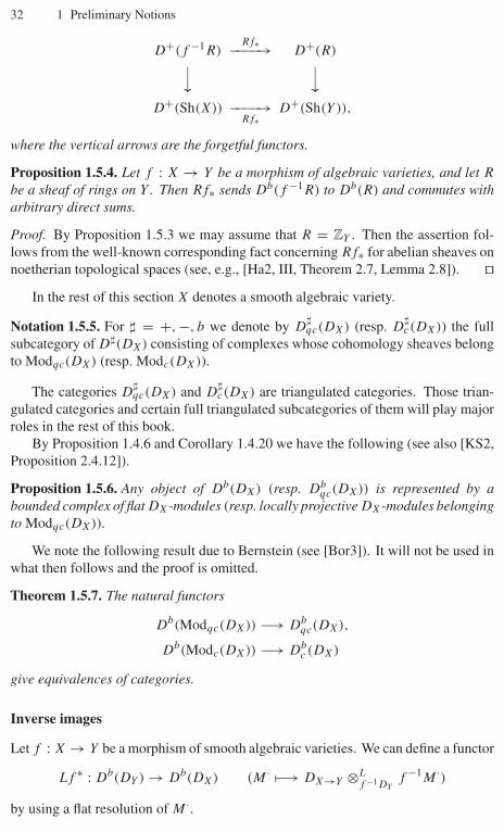
32 1 Preliminary Notions
D+(f −1R)Rf∗−−−−→ D+(R)⏐⏐ ⏐⏐
D+(Sh(X)) −−−−→Rf∗
D+(Sh(Y )),
where the vertical arrows are the forgetful functors.
Proposition 1.5.4. Let f : X → Y be a morphism of algebraic varieties, and let R
be a sheaf of rings on Y . Then Rf∗ sends Db(f −1R) to Db(R) and commutes witharbitrary direct sums.
Proof. By Proposition 1.5.3 we may assume that R = ZY . Then the assertion fol-lows from the well-known corresponding fact concerning Rf∗ for abelian sheaves onnoetherian topological spaces (see, e.g., [Ha2, III, Theorem 2.7, Lemma 2.8]). ��
In the rest of this section X denotes a smooth algebraic variety.
Notation 1.5.5. For � = +, −, b we denote by D�qc(DX) (resp. D
�c(DX)) the full
subcategory of D�(DX) consisting of complexes whose cohomology sheaves belongto Modqc(DX) (resp. Modc(DX)).
The categories D�qc(DX) and D
�c(DX) are triangulated categories. Those trian-
gulated categories and certain full triangulated subcategories of them will play majorroles in the rest of this book.
By Proposition 1.4.6 and Corollary 1.4.20 we have the following (see also [KS2,Proposition 2.4.12]).
Proposition 1.5.6. Any object of Db(DX) (resp. Dbqc(DX)) is represented by a
bounded complex of flat DX-modules (resp. locally projective DX-modules belongingto Modqc(DX)).
We note the following result due to Bernstein (see [Bor3]). It will not be used inwhat then follows and the proof is omitted.
Theorem 1.5.7. The natural functors
Db(Modqc(DX)) −→ Dbqc(DX),
Db(Modc(DX)) −→ Dbc (DX)
give equivalences of categories.
Inverse images
Let f : X → Y be a morphism of smooth algebraic varieties. We can define a functor
Lf ∗ : Db(DY ) → Db(DX) (M · �−→ DX→Y ⊗Lf −1DY
f −1M ·)
by using a flat resolution of M ·.
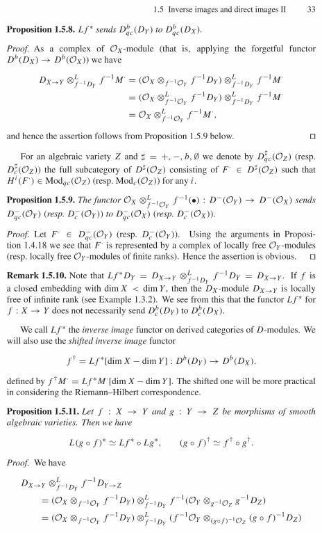
1.5 Inverse images and direct images II 33
Proposition 1.5.8. Lf ∗ sends Dbqc(DY ) to Db
qc(DX).
Proof. As a complex of OX-module (that is, applying the forgetful functorDb(DX) → Db(OX)) we have
DX→Y ⊗Lf −1DY
f −1M · = (OX ⊗f −1OYf −1DY ) ⊗L
f −1DYf −1M ·
= (OX ⊗Lf −1OY
f −1DY ) ⊗Lf −1DY
f −1M ·
= OX ⊗Lf −1OY
f −1M ·,
and hence the assertion follows from Proposition 1.5.9 below. ��For an algebraic variety Z and � = +, −, b, ∅ we denote by D
�qc(OZ) (resp.
D�c(OZ)) the full subcategory of D�(OZ) consisting of F · ∈ D�(OZ) such that
Hi(F ·) ∈ Modqc(OZ) (resp. Modc(OZ)) for any i.
Proposition 1.5.9. The functor OX ⊗Lf −1OY
f −1(•) : D−(OY ) → D−(OX) sends
D−qc(OY ) (resp. D−
c (OY )) to D−qc(OX) (resp. D−
c (OX)).
Proof. Let F · ∈ D−qc(OY ) (resp. D−
c (OY )). Using the arguments in Proposi-tion 1.4.18 we see that F · is represented by a complex of locally free OY -modules(resp. locally free OY -modules of finite ranks). Hence the assertion is obvious. ��Remark 1.5.10. Note that Lf ∗DY = DX→Y ⊗L
f −1DYf −1DY = DX→Y . If f is
a closed embedding with dim X < dim Y , then the DX-module DX→Y is locallyfree of infinite rank (see Example 1.3.2). We see from this that the functor Lf ∗ forf : X → Y does not necessarily send Db
c (DY ) to Dbc (DX).
We call Lf ∗ the inverse image functor on derived categories of D-modules. Wewill also use the shifted inverse image functor
f † = Lf ∗[dim X − dim Y ] : Db(DY ) → Db(DX).
defined by f †M · = Lf ∗M ·[dim X − dim Y ]. The shifted one will be more practicalin considering the Riemann–Hilbert correspondence.
Proposition 1.5.11. Let f : X → Y and g : Y → Z be morphisms of smoothalgebraic varieties. Then we have
L(g ◦ f )∗ � Lf ∗ ◦ Lg∗, (g ◦ f )† � f † ◦ g†.
Proof. We have
DX→Y ⊗Lf −1DY
f −1DY→Z
= (OX ⊗f −1OYf −1DY ) ⊗L
f −1DYf −1(OY ⊗g−1OZ
g−1DZ)
= (OX ⊗f −1OYf −1DY ) ⊗L
f −1DY(f −1OY ⊗(g◦f )−1OZ
(g ◦ f )−1DZ)

34 1 Preliminary Notions
= (OX ⊗Lf −1OY
f −1DY ) ⊗Lf −1DY
(f −1OY ⊗L(g◦f )−1OZ
(g ◦ f )−1DZ)
� OX ⊗L(g◦f )−1OZ
(g ◦ f )−1DZ
= OX ⊗(g◦f )−1OZ(g ◦ f )−1DZ
= DX→Z.
Here we have used the fact the D is a locally free O-module. Hence we obtainisomorphisms
DX→Z � DX→Y ⊗f −1DYf −1DY→Z � DX→Y ⊗L
f −1DYf −1DY→Z
of (complexes of) (DX, (g ◦ f )−1DZ)-bimodules. Therefore, we have
L(g ◦ f )∗(M.) = DX→Z ⊗L(g◦f )−1DY
(g ◦ f )−1M.
� (DX→Y ⊗Lf −1DY
f −1DY→Z) ⊗Lf −1g−1DY
f −1g−1M.
= DX→Y ⊗Lf −1DY
f −1(DY→Z ⊗Lg−1DY
g−1M.)
= Lf ∗(Lg∗(M.)).
This completes the proof. ��Example 1.5.12. Assume that U is an open subset of a smooth algebraic variety X.Let j : U ↪→ X be the embedding. Then we have DU→X = j−1DX = DU andhence
j† = Lj∗ = j−1 (the restriction to U).
Proposition 1.5.13. Assume that f : X → Y is a smooth morphism between smoothalgebraic varieties.
(i) For M ∈ Mod(DY ) we have Hi(Lf ∗M) = 0 for i = 0 (hence we write f ∗ forLf ∗ in this case).
(ii) For M ∈ Modc(DY ) we have f ∗M ∈ Modc(DX).
Proof. (i) The assertion follows from the flatness of OX over f −1OY and Lf ∗M �OX ⊗L
f −1OYf −1M .
(ii) It is sufficient to show that the canonical morphism DX → DX→Y =OX ⊗f −1OY
f −1DY (P �→ P(1 ⊗ 1)) is surjective. Since the question is local,we may assume that X and Y are affine and admit local coordinates {xi, ∂xi
}i=1,...,n
and {yi, ∂yi}i=1,...,m, respectively, such that
∂xi�→{
1 ⊗ ∂yi(1 ≤ i ≤ m)
0 (m + 1 ≤ i ≤ n)
under the canonical morphism �X → f ∗�Y = OX ⊗f −1OYf −1�Y . Then we have
DX→Y =⊕
r1,...,rm
OX∂r1y1
· · · ∂rmym
,
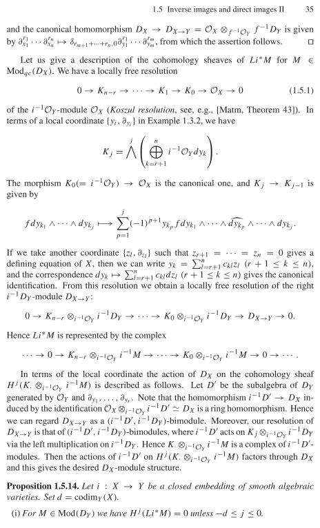
1.5 Inverse images and direct images II 35
and the canonical homomorphism DX → DX→Y = OX ⊗f −1OYf −1DY is given
by ∂r1x1 · · · ∂rn
xn�→ δrm+1+···+rn,0∂
r1y1 · · · ∂rm
ym, from which the assertion follows. ��
Let us give a description of the cohomology sheaves of Li∗M for M ∈Modqc(DX). We have a locally free resolution
0 → Kn−r → · · · → K1 → K0 → OX → 0 (1.5.1)
of the i−1OY -module OX (Koszul resolution, see, e.g., [Matm, Theorem 43]). Interms of a local coordinate {yi, ∂yi
} in Example 1.3.2, we have
Kj =j∧⎛⎝ n⊕
k=r+1
i−1OY dyk
⎞⎠ .
The morphism K0(= i−1OY ) → OX is the canonical one, and Kj → Kj−1 isgiven by
f dyk1 ∧ · · · ∧ dykj�−→
j∑p=1
(−1)p+1ykpf dyk1 ∧ · · · ∧ dykp ∧ · · · ∧ dykj.
If we take another coordinate {zl, ∂zl} such that zr+1 = · · · = zn = 0 gives a
defining equation of X, then we can write yk = ∑nl=r+1 cklzl (r + 1 ≤ k ≤ n),
and the correspondence dyk �→ ∑nl=r+1 ckldzl (r + 1 ≤ k ≤ n) gives the canonical
identification. From this resolution we obtain a locally free resolution of the righti−1DY -module DX→Y :
0 → Kn−r ⊗i−1OYi−1DY → · · · → K0 ⊗i−1OY
i−1DY → DX→Y → 0.
Hence Li∗M is represented by the complex
· · · → 0 → Kn−r ⊗i−1OYi−1M → · · · → K0 ⊗i−1OY
i−1M → 0 → · · · .
In terms of the local coordinate the action of DX on the cohomology sheafHj (K· ⊗i−1OY
i−1M) is described as follows. Let D′ be the subalgebra of DY
generated by OY and ∂y1 , . . . , ∂yr . Note that the homomorphism i−1D′ → DX in-duced by the identification OX ⊗i−1OY
i−1D′ � DX is a ring homomorphism. Hencewe can regard DX→Y as a (i−1D′, i−1DY )-bimodule. Moreover, our resolution ofDX→Y is that of (i−1D′, i−1DY )-bimodules, where i−1D′ acts on Kj ⊗i−1OY
i−1DY
via the left multiplication on i−1DY . Hence K· ⊗i−1OYi−1M is a complex of i−1D′-
modules. Then the actions of i−1D′ on Hj (K· ⊗i−1OYi−1M) factors through DX
and this gives the desired DX-module structure.
Proposition 1.5.14. Let i : X → Y be a closed embedding of smooth algebraicvarieties. Set d = codimY (X).
(i) For M ∈ Mod(DY ) we have Hj (Li∗M) = 0 unless −d ≤ j ≤ 0.
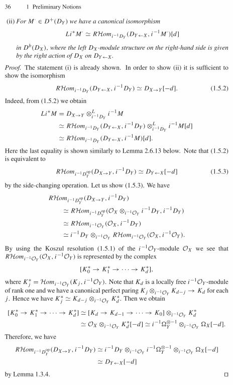
36 1 Preliminary Notions
(ii) For M · ∈ D+(DY ) we have a canonical isomorphism
Li∗M · � RHomi−1DY(DY←X, i−1M ·)[d]
in Db(DX), where the left DX-module structure on the right-hand side is givenby the right action of DX on DY←X.
Proof. The statement (i) is already shown. In order to show (ii) it is sufficient toshow the isomorphism
RHomi−1DY(DY←X, i−1DY ) � DX→Y [−d]. (1.5.2)
Indeed, from (1.5.2) we obtain
Li∗M = DX→Y ⊗Li−1DY
i−1M
� RHomi−1DY(DY←X, i−1DY ) ⊗L
i−1DYi−1M[d]
� RHomi−1DY(DY←X, i−1M)[d].
Here the last equality is shown similarly to Lemma 2.6.13 below. Note that (1.5.2)is equivalent to
RHomi−1DopY
(DX→Y , i−1DY ) � DY←X[−d] (1.5.3)
by the side-changing operation. Let us show (1.5.3). We have
RHomi−1DopY
(DX→Y , i−1DY )
� RHomi−1DopY
(OX ⊗i−1OYi−1DY , i−1DY )
� RHomi−1OY(OX, i−1DY )
� i−1DY ⊗i−1OYRHomi−1OY
(OX, i−1OY ).
By using the Koszul resolution (1.5.1) of the i−1OY -module OX we see thatRHomi−1OY
(OX, i−1OY ) is represented by the complex
[K∗0 → K∗
1 → · · · → K∗d ],
where K∗j = Homi−1OY
(Kj , i−1OY ). Note that Kd is a locally free i−1OY -moduleof rank one and we have a canonical perfect paring Kj ⊗i−1OY
Kd−j → Kd for eachj . Hence we have K∗
j � Kd−j ⊗i−1OYK∗
d . Then we obtain
[K∗0 → K∗
1 → · · · → K∗d ] � [Kd → Kd−1 → · · · → K0] ⊗i−1OY
K∗d
� OX ⊗i−1OYK∗
d [−d] � i−1�⊗−1Y ⊗i−1OY
�X[−d].Therefore, we have
RHomi−1DopY
(DX→Y , i−1DY ) � i−1DY ⊗i−1OYi−1�⊗−1
Y ⊗i−1OY�X[−d]
� DY←X[−d]by Lemma 1.3.4. ��
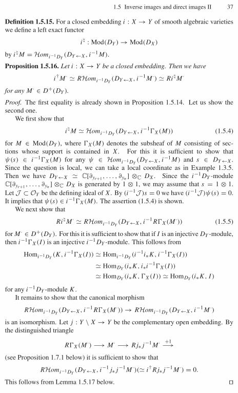
1.5 Inverse images and direct images II 37
Definition 1.5.15. For a closed embedding i : X → Y of smooth algebraic varietieswe define a left exact functor
i� : Mod(DY ) → Mod(DX)
by i�M = Homi−1DY(DY←X, i−1M).
Proposition 1.5.16. Let i : X → Y be a closed embedding. Then we have
i†M · � RHomi−1DY(DY←X, i−1M ·) � Ri�M ·
for any M · ∈ D+(DY ).
Proof. The first equality is already shown in Proposition 1.5.14. Let us show thesecond one.
We first show that
i�M � Homi−1DY(DY←X, i−1�X(M)) (1.5.4)
for M ∈ Mod(DY ), where �X(M) denotes the subsheaf of M consisting of sec-tions whose support is contained in X. For this it is sufficient to show thatψ(s) ∈ i−1�X(M) for any ψ ∈ Homi−1DY
(DY←X, i−1M) and s ∈ DY←X.Since the question is local, we can take a local coordinate as in Example 1.3.5.Then we have DY←X � C[∂yr+1 , . . . , ∂yn ] ⊗C DX. Since the i−1DY -moduleC[∂yr+1 , . . . , ∂yn ] ⊗C DX is generated by 1 ⊗ 1, we may assume that s = 1 ⊗ 1.Let J ⊂ OY be the defining ideal of X. By (i−1J )s = 0 we have (i−1J )ψ(s) = 0.It implies that ψ(s) ∈ i−1�X(M). The assertion (1.5.4) is shown.
We next show that
Ri�M · � RHomi−1DY(DY←X, i−1R�X(M ·)) (1.5.5)
for M · ∈ D+(DY ). For this it is sufficient to show that if I is an injective DY -module,then i−1�X(I) is an injective i−1DY -module. This follows from
Homi−1DY(K, i−1�X(I)) � Homi−1DY
(i−1i∗K, i−1�X(I))
� HomDY(i∗K, i∗i−1�X(I))
� HomDY(i∗K, �X(I)) � HomDY
(i∗K, I)
for any i−1DY -module K .It remains to show that the canonical morphism
RHomi−1DY(DY←X, i−1R�X(M ·)) → RHomi−1DY
(DY←X, i−1M ·)
is an isomorphism. Let j : Y \ X → Y be the complementary open embedding. Bythe distinguished triangle
R�X(M ·) −→ M · −→ Rj∗j−1M · +1−→(see Proposition 1.7.1 below) it is sufficient to show that
RHomi−1DY(DY←X, i−1j∗j−1M ·)(� i†Rj∗j−1M ·) = 0.
This follows from Lemma 1.5.17 below. ��
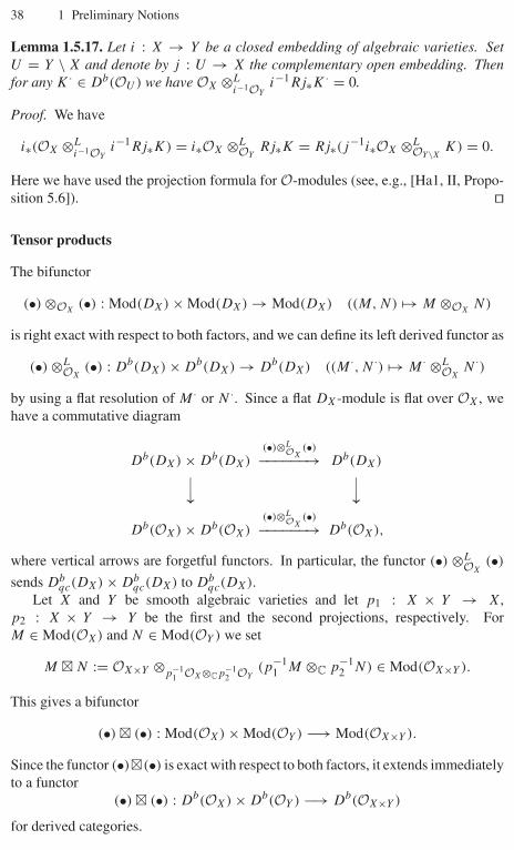
38 1 Preliminary Notions
Lemma 1.5.17. Let i : X → Y be a closed embedding of algebraic varieties. SetU = Y \ X and denote by j : U → X the complementary open embedding. Thenfor any K · ∈ Db(OU ) we have OX ⊗L
i−1OYi−1Rj∗K · = 0.
Proof. We have
i∗(OX ⊗Li−1OY
i−1Rj∗K) = i∗OX ⊗LOY
Rj∗K = Rj∗(j−1i∗OX ⊗LOY\X
K) = 0.
Here we have used the projection formula for O-modules (see, e.g., [Ha1, II, Propo-sition 5.6]). ��
Tensor products
The bifunctor
(•) ⊗OX(•) : Mod(DX) × Mod(DX) → Mod(DX) ((M, N) �→ M ⊗OX
N)
is right exact with respect to both factors, and we can define its left derived functor as
(•) ⊗LOX
(•) : Db(DX) × Db(DX) → Db(DX) ((M ·, N ·) �→ M · ⊗LOX
N ·)
by using a flat resolution of M · or N ·. Since a flat DX-module is flat over OX, wehave a commutative diagram
Db(DX) × Db(DX)(•)⊗L
OX(•)
−−−−−−→ Db(DX)⏐⏐ ⏐⏐Db(OX) × Db(OX)
(•)⊗LOX
(•)
−−−−−−→ Db(OX),
where vertical arrows are forgetful functors. In particular, the functor (•) ⊗LOX
(•)
sends Dbqc(DX) × Db
qc(DX) to Dbqc(DX).
Let X and Y be smooth algebraic varieties and let p1 : X × Y → X,p2 : X × Y → Y be the first and the second projections, respectively. ForM ∈ Mod(OX) and N ∈ Mod(OY ) we set
M � N := OX×Y ⊗p−1
1 OX⊗Cp−12 OY
(p−11 M ⊗C p−1
2 N) ∈ Mod(OX×Y ).
This gives a bifunctor
(•) � (•) : Mod(OX) × Mod(OY ) −→ Mod(OX×Y ).
Since the functor (•)�(•) is exact with respect to both factors, it extends immediatelyto a functor
(•) � (•) : Db(OX) × Db(OY ) −→ Db(OX×Y )
for derived categories.
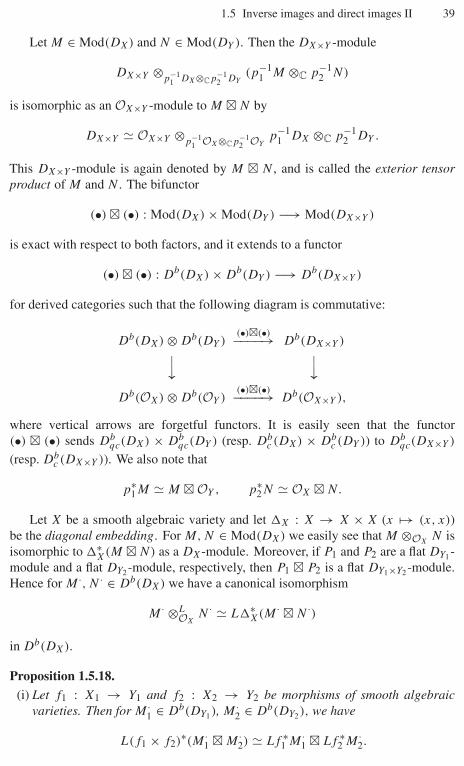
1.5 Inverse images and direct images II 39
Let M ∈ Mod(DX) and N ∈ Mod(DY ). Then the DX×Y -module
DX×Y ⊗p−1
1 DX⊗Cp−12 DY
(p−11 M ⊗C p−1
2 N)
is isomorphic as an OX×Y -module to M � N by
DX×Y � OX×Y ⊗p−1
1 OX⊗Cp−12 OY
p−11 DX ⊗C p−1
2 DY .
This DX×Y -module is again denoted by M � N , and is called the exterior tensorproduct of M and N . The bifunctor
(•) � (•) : Mod(DX) × Mod(DY ) −→ Mod(DX×Y )
is exact with respect to both factors, and it extends to a functor
(•) � (•) : Db(DX) × Db(DY ) −→ Db(DX×Y )
for derived categories such that the following diagram is commutative:
Db(DX) ⊗ Db(DY )(•)�(•)−−−−→ Db(DX×Y )⏐⏐ ⏐⏐
Db(OX) ⊗ Db(OY )(•)�(•)−−−−→ Db(OX×Y ),
where vertical arrows are forgetful functors. It is easily seen that the functor(•) � (•) sends Db
qc(DX) × Dbqc(DY ) (resp. Db
c (DX) × Dbc (DY )) to Db
qc(DX×Y )
(resp. Dbc (DX×Y )). We also note that
p∗1M � M � OY , p∗
2N � OX � N.
Let X be a smooth algebraic variety and let �X : X → X × X (x �→ (x, x))be the diagonal embedding. For M, N ∈ Mod(DX) we easily see that M ⊗OX
N isisomorphic to �∗
X(M � N) as a DX-module. Moreover, if P1 and P2 are a flat DY1 -module and a flat DY2 -module, respectively, then P1 � P2 is a flat DY1×Y2 -module.Hence for M ·, N · ∈ Db(DX) we have a canonical isomorphism
M · ⊗LOX
N · � L�∗X(M · � N ·)
in Db(DX).
Proposition 1.5.18.(i) Let f1 : X1 → Y1 and f2 : X2 → Y2 be morphisms of smooth algebraic
varieties. Then for M ·1 ∈ Db(DY1), M ·
2 ∈ Db(DY2), we have
L(f1 × f2)∗(M ·1 � M ·
2) � Lf ∗1 M ·
1 � Lf ∗2 M ·
2.
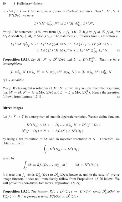
40 1 Preliminary Notions
(ii) Let f : X → Y be a morphism of smooth algebraic varieties. Then for M ·, N · ∈Db(DY ), we have
Lf ∗(M · ⊗LOY
N ·) � Lf ∗M · ⊗LOX
Lf ∗N ·.
Proof. The statement (i) follows from (f1 × f2)∗(M1 � M2) � f ∗1 M1 � f ∗
2 M2 forM1 ∈ Mod(DY1), M2 ∈ Mod(DY2). The statement (ii) follows from (i) as follows:
Lf ∗(M · ⊗LOY
N ·) � Lf ∗L�∗Y (M · � N ·) � L�∗
XL(f × f )∗(M · � N ·)
� L�∗X(Lf ∗M · � Lf ∗N ·) � Lf ∗M · ⊗L
OXLf ∗N ·. ��
Proposition 1.5.19. Let M ·, N · ∈ Db(DX) and L· ∈ Db(DopX ). Then we have
isomorphisms
(L· ⊗LOX
N ·) ⊗LDX
M · � L· ⊗LDX
(M · ⊗LOX
N ·) � (L· ⊗LOX
M ·) ⊗LDX
N ·
of CX-modules.
Proof. By taking flat resolutions of M ·, N ·, L· we may assume from the beginningthat M · = M, N · = N ∈ Mod(DX) and L· = L ∈ Mod(D
opX ). Hence the assertion
follows from Lemma 1.2.11. ��
Direct images
Let f : X → Y be a morphism of smooth algebraic varieties. We can define functors
Db(DX) M · �−→ DY←X ⊗LDX
M · ∈ Db(f −1DY ),
Db(f −1DY ) N · �−→ Rf∗(N ·) ∈ Db(DY )
by using a flat resolution of M · and an injective resolution of N ·. Therefore, weobtain a functor ∫
f
: Db(DX) → Db(DY )
given by ∫f
M. = Rf∗(DY←X ⊗LDX
M.) (M. ∈ Db(DX)).
It is true that∫
fsends Db
qc(DX) to Dbqc(DY ); however, unlike the case of inverse
image functors it does not immediately follow from Proposition 1.5.20 below. Wewill prove this non-trivial fact later (Proposition 1.5.29).
Proposition 1.5.20. The functor Rf∗ : Db(OX) → Db(OY ) sends Dbqc(OX) to
Dbqc(OY ). If f is proper, it sends Db
c (OX) to Dbc (OY ).
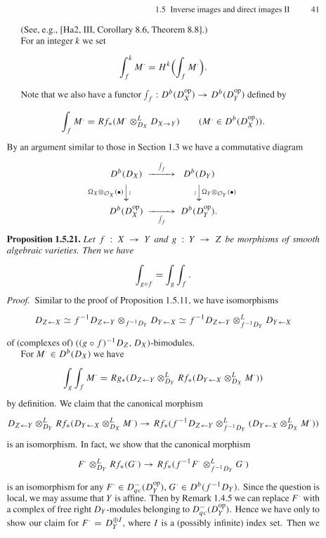
1.5 Inverse images and direct images II 41
(See, e.g., [Ha2, III, Corollary 8.6, Theorem 8.8].)For an integer k we set ∫ k
f
M · = Hk(∫
f
M ·).Note that we also have a functor
∫f
: Db(DopX ) → Db(D
opY ) defined by∫
f
M. = Rf∗(M · ⊗LDX
DX→Y ) (M. ∈ Db(DopX )).
By an argument similar to those in Section 1.3 we have a commutative diagram
Db(DX)
∫f−−−−→ Db(DY )
�X⊗OX(•)
⏐⏐� �⏐⏐�Y ⊗OY
(•)
Db(DopX ) −−−−→∫
f
Db(DopY ).
Proposition 1.5.21. Let f : X → Y and g : Y → Z be morphisms of smoothalgebraic varieties. Then we have ∫
g◦f
=∫
g
∫f
.
Proof. Similar to the proof of Proposition 1.5.11, we have isomorphisms
DZ←X � f −1DZ←Y ⊗f −1DYDY←X � f −1DZ←Y ⊗L
f −1DYDY←X
of (complexes of) ((g ◦ f )−1DZ, DX)-bimodules.For M · ∈ Db(DX) we have∫
g
∫f
M · = Rg∗(DZ←Y ⊗LDY
Rf∗(DY←X ⊗LDX
M ·))
by definition. We claim that the canonical morphism
DZ←Y ⊗LDY
Rf∗(DY←X ⊗LDX
M ·) → Rf∗(f −1DZ←Y ⊗Lf −1DY
(DY←X ⊗LDX
M ·))
is an isomorphism. In fact, we show that the canonical morphism
F · ⊗LDY
Rf∗(G·) → Rf∗(f −1F · ⊗Lf −1DY
G·)
is an isomorphism for any F · ∈ D−qc(D
opY ), G· ∈ Db(f −1DY ). Since the question is
local, we may assume that Y is affine. Then by Remark 1.4.5 we can replace F · witha complex of free right DY -modules belonging to D−
qc(DopY ). Hence we have only to
show our claim for F · = D⊕IY , where I is a (possibly infinite) index set. Then we
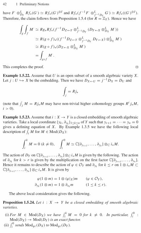
42 1 Preliminary Notions
have F · ⊗LDY
Rf∗(G·) � Rf∗(G·)⊕I and Rf∗(f −1F · ⊗Lf −1DY
G·) � Rf∗((G·)⊕I ).Therefore, the claim follows from Proposition 1.5.4 (for R = ZY ). Hence we have∫
g
∫f
M · � Rg∗Rf∗(f −1DZ←Y ⊗Lf −1DY
(DY←X ⊗LDX
M ·))
� R(g ◦ f )∗((f −1DZ←Y ⊗Lf −1DY
DY←X) ⊗LDX
M ·)
� R(g ◦ f )∗(DZ←X ⊗LDX
M ·)
=∫
g◦f
M ·.
This completes the proof. ��Example 1.5.22. Assume that U is an open subset of a smooth algebraic variety X.Let j : U ↪→ X be the embedding. Then we have DX←U = j−1DX = DU and∫
j
= Rj∗
(note that∫
jM = Rj∗M may have non-trivial higher cohomology groups Rij∗M ,
i > 0).
Example 1.5.23. Assume that i : X → Y is a closed embedding of smooth algebraicvarieties. Take a local coordinate {yk, ∂yk
}1≤k≤n of Y such that yr+1 = · · · = yn = 0gives a defining equation of X. By Example 1.3.5 we have the following localdescription of
∫iM for M ∈ Mod(DX):∫ k
i
M = 0 (k = 0),
∫ 0
i
M � C[∂yr+1 , . . . , ∂yn ] ⊗C i∗M.
The action of DY on C[∂yr+1 , . . . , ∂yn ]⊗C i∗M is given by the following. The actionof ∂yk
for k > r is given by the multiplication on the first factor C[∂yr+1 , . . . , ∂yn ].Hence it remains to describe the action of ϕ ∈ OY and ∂yk
for k ≤ r on 1 ⊗ i∗M ⊂C[∂yr+1 , . . . , ∂yn ] ⊗C i∗M . It is given by
ϕ(1 ⊗ m) = 1 ⊗ (ϕ|X)m (ϕ ∈ OY ),
∂yk(1 ⊗ m) = 1 ⊗ ∂xk
m (1 ≤ k ≤ r).
The above local consideration gives the following.
Proposition 1.5.24. Let i : X → Y be a closed embedding of smooth algebraicvarieties.
(i) For M ∈ Mod(DX) we have∫ k
iM = 0 for k = 0. In particular,
∫ 0i
:Mod(DX) → Mod(DY ) is an exact functor.
(ii)∫ 0
isends Modqc(DX) to Modqc(DY ).
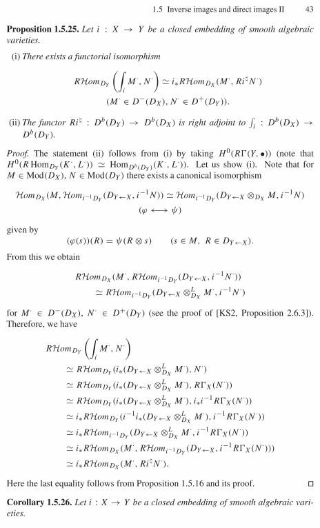
1.5 Inverse images and direct images II 43
Proposition 1.5.25. Let i : X → Y be a closed embedding of smooth algebraicvarieties.
(i) There exists a functorial isomorphism
RHomDY
(∫i
M ·, N ·)
� i∗RHomDX(M ·, Ri�N ·)
(M · ∈ D−(DX), N · ∈ D+(DY )).
(ii) The functor Ri� : Db(DY ) → Db(DX) is right adjoint to∫
i: Db(DX) →
Db(DY ).
Proof. The statement (ii) follows from (i) by taking H 0(R�(Y, •)) (note thatH 0(R HomDY
(K ·, L·)) � HomDb(DY )(K·, L·)). Let us show (i). Note that for
M ∈ Mod(DX), N ∈ Mod(DY ) there exists a canonical isomorphism
HomDX(M, Homi−1DY
(DY←X, i−1N)) � Homi−1DY(DY←X ⊗DX
M, i−1N)
(ϕ ←→ ψ)
given by(ϕ(s))(R) = ψ(R ⊗ s) (s ∈ M, R ∈ DY←X).
From this we obtain
RHomDX(M ·, RHomi−1DY
(DY←X, i−1N ·))� RHomi−1DY
(DY←X ⊗LDX
M ·, i−1N ·)
for M · ∈ D−(DX), N · ∈ D+(DY ) (see the proof of [KS2, Proposition 2.6.3]).Therefore, we have
RHomDY
(∫i
M ·, N ·)
� RHomDY(i∗(DY←X ⊗L
DXM ·), N ·)
� RHomDY(i∗(DY←X ⊗L
DXM ·), R�X(N ·))
� RHomDY(i∗(DY←X ⊗L
DXM ·), i∗i−1R�X(N ·))
� i∗RHomDY(i−1i∗(DY←X ⊗L
DXM ·), i−1R�X(N ·))
� i∗RHomi−1DY(DY←X ⊗L
DXM ·, i−1R�X(N ·))
� i∗RHomDX(M ·, RHomi−1DY
(DY←X, i−1R�X(N ·)))� i∗RHomDX
(M ·, Ri�N ·).
Here the last equality follows from Proposition 1.5.16 and its proof. ��Corollary 1.5.26. Let i : X → Y be a closed embedding of smooth algebraic vari-eties.
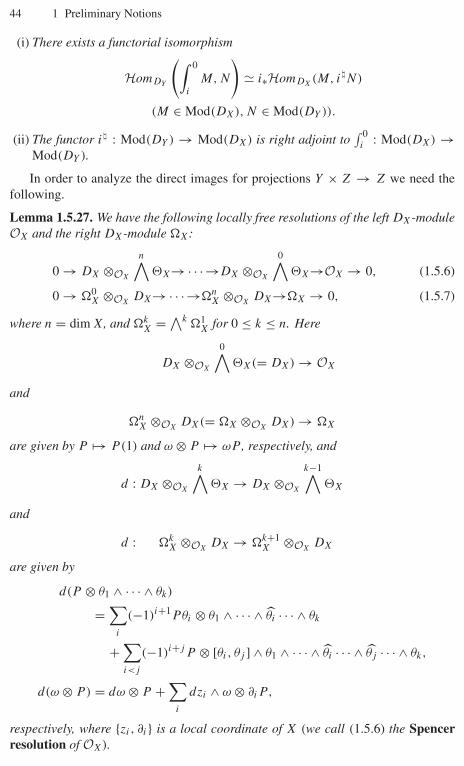
44 1 Preliminary Notions
(i) There exists a functorial isomorphism
HomDY
(∫ 0
i
M, N
)� i∗HomDX
(M, i�N)
(M ∈ Mod(DX), N ∈ Mod(DY )).
(ii) The functor i� : Mod(DY ) → Mod(DX) is right adjoint to∫ 0
i: Mod(DX) →
Mod(DY ).
In order to analyze the direct images for projections Y × Z → Z we need thefollowing.
Lemma 1.5.27. We have the following locally free resolutions of the left DX-moduleOX and the right DX-module �X:
0 → DX ⊗OX
n∧�X→ · · · →DX ⊗OX
0∧�X→OX → 0, (1.5.6)
0 → �0X ⊗OX
DX→ · · · →�nX ⊗OX
DX→�X → 0, (1.5.7)
where n = dim X, and �kX = ∧k
�1X for 0 ≤ k ≤ n. Here
DX ⊗OX
0∧�X(= DX) → OX
and
�nX ⊗OX
DX(= �X ⊗OXDX) → �X
are given by P �→ P(1) and ω ⊗ P �→ ωP , respectively, and
d : DX ⊗OX
k∧�X → DX ⊗OX
k−1∧�X
and
d : �kX ⊗OX
DX → �k+1X ⊗OX
DX
are given by
d(P ⊗ θ1 ∧ · · · ∧ θk)
=∑
i
(−1)i+1Pθi ⊗ θ1 ∧ · · · ∧ θi · · · ∧ θk
+∑i<j
(−1)i+j P ⊗ [θi, θj ] ∧ θ1 ∧ · · · ∧ θi · · · ∧ θj · · · ∧ θk,
d(ω ⊗ P) = dω ⊗ P +∑
i
dzi ∧ ω ⊗ ∂iP ,
respectively, where {zi, ∂i} is a local coordinate of X (we call (1.5.6) the Spencerresolution of OX).
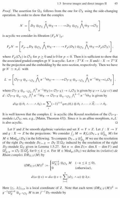
1.5 Inverse images and direct images II 45
Proof. The assertion for �X follows from the one for OX using the side-changingoperation. In order to show that the complex
N · =[
DX ⊗OX
n∧�X→ · · · →DX ⊗OX
0∧�X→OX
]is acyclic we consider its filtration {FpN ·}p:
FpN · =[
Fp−nDX ⊗OX
n∧�X→ · · · →Fp(DX) ⊗OX
0∧�X→Fp(OX)
],
where Fp(OX) is OX for p ≥ 0 and is 0 for p < 0. Then it is sufficient to show thatthe associated graded complex gr N · is acyclic. Let π : T ∗X → X and i : X → T ∗X
be the projection and the embedding by the zero-section, respectively. Then we havegr N · � π∗L· with
L· =[OT ∗X ⊗π−1OX
n∧π−1�X→ · · · →OT ∗X ⊗π−1OX
0∧π−1�X→i∗OX
],
where OT ∗X ⊗π−1OX
∧0π−1�X(= OT ∗X) → i∗OX is given by ϕ �→ i∗(ϕ ◦ i) and
d : OT ∗X ⊗π−1OX
∧kπ−1�X → OT ∗X ⊗π−1OX
∧k−1π−1�X is given by
d(ϕ ⊗ θ1 ∧ · · · ∧ θk) =∑
i
(−1)i+1ϕσ1(θi) ⊗ θ1 ∧ · · · ∧ θi · · · ∧ θk.
It is well known that the complex L· is acyclic (the Koszul resolution of the OT ∗X-module i∗OX; see, e.g., [Matm, Theorem 43]). Since π is an affine morphism, π∗L·is also acyclic. ��
Let Y and Z be smooth algebraic varieties and set X = Y × Z. Let f : X → Y
and g : X → Z be the projections. We consider∫
fM = Rf∗(DY←X ⊗L
DXM) for
M ∈ Modqc(DX) in the following. To compute DY←X ⊗LDX
M we use the resolutionof the right DX-module DY←X = DY � �Z induced by the resolution of the rightDZ-module �Z given in Lemma 1.5.27. Set n = dim Z(= dim X − dim Y ) and�k
X/Y = OY � �kZ for 0 ≤ k ≤ n. For M ∈ Modqc(DX) we define its (relative) de
Rham complex DRX/Y (M) by
(DRX/Y (M))k :={
�n+kX/Y ⊗OX
M (−n ≤ k ≤ 0),
0 (otherwise),
d(ω ⊗ s) = dω ⊗ s +n∑
i=1
(dzi ∧ ω) ⊗ ∂is.
Here {zi, ∂i}1≤n is a local coordinate of Z. Note that each term (DRX/Y (M))k =g−1�n+k
Z ⊗g−1OZM is an f −1DY -module by
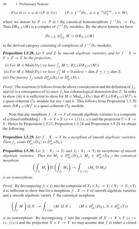
46 1 Preliminary Notions
P(ω ⊗ s) = ω ⊗ ((P ⊗ 1)s) (P ∈ f −1DY , ω ∈ g−1�n+kZ , s ∈ M),
where we denote by P �→ P ⊗ 1 the canonical homomorphism f −1DY → DX.Thus DRX/Y (M) is a complex of f −1DY -modules. By the above lemma we have
DY←X ⊗LDX
M � DRX/Y (M)
in the derived category consisting of complexes of f −1DY -modules.
Proposition 1.5.28. Let Y and Z be smooth algebraic varieties, and let f : X =Y × Z → Y be the projection.
(i) For M ∈ Mod(DX) we have∫
fM � Rf∗(DRX/Y (M)).
(ii) For M ∈ Mod(DX) we have∫ j
fM = 0 unless − dim Z ≤ j ≤ dim Z.
(iii) The functor∫
fsends Db
qc(DX) to Dbqc(DY ).
Proof. The assertion (i) follows from the above consideration and the definition of∫
f,
and (ii) is a consequence of (i) since f∗ has cohomological dimension dim Z. In orderto show (iii) it is sufficient to show for M ∈ Modqc(DX) that Rif∗(DRX/Y (M)k) isa quasi-coherent OY -module for any i and k. This follows from Proposition 1.5.20since DRX/Y (M)k is a quasi-coherent OX-module. ��
Note that any morphism f : X → Y of smooth algebraic varieties is a compositeof a closed embedding i : X → Y ×X (x �→ (f (x), x)) and the projection Y ×X →Y . Hence by Proposition 1.5.21, Proposition 1.5.24 and Proposition 1.5.28 we obtainthe following.
Proposition 1.5.29. Let f : X → Y be a morphism of smooth algebraic varieties.Then
∫f
sends Dbqc(DX) to Db
qc(DY ).
Proposition 1.5.30. Let f1 : X1 → Y1 and f2 : X2 → Y2 be morphisms of smoothalgebraic varieties. Then for M ·
1 ∈ Dbqc(DX1), M ·
2 ∈ Dbqc(DX2) the canonical
morphism (∫f1
M ·1
)�(∫
f2
M ·2
)→∫
f1×f2
(M ·1 � M ·
2)
is an isomorphism.
Proof. By decomposing f1×f2 into the composite of X1×X2 → Y1×X2 → Y1×Y2it is sufficient to show that for a morphism f : X → Y of smooth algebraic varietiesand a smooth algebraic variety T the canonical morphism(∫
f
M ·)
� N · →∫
f ×idT
(M · � N ·) (M ∈ Dbqc(DX), N ∈ Db
qc(T ))
is an isomorphism. By decomposing f into the composite of X → X × Y (x �→(x, f (x)) and the projection X × Y → Y we may assume that f is either a closed
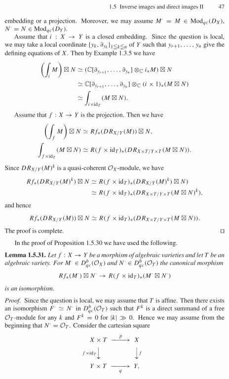
1.5 Inverse images and direct images II 47
embedding or a projection. Moreover, we may assume M · = M ∈ Modqc(DX),N · = N ∈ Modqc(DY ).
Assume that i : X → Y is a closed embedding. Since the question is local,we may take a local coordinate {yk, ∂yk
}1�k�n of Y such that yr+1, . . . , yn give thedefining equations of X. Then by Example 1.3.5 we have(∫
i
M
)� N � (C[∂yr+1 , . . . , ∂yn ] ⊗C i∗M) � N
� C[∂yr+1 , . . . , ∂yn ] ⊗C (i × 1)∗(M � N)
�∫
i×idT
(M � N).
Assume that f : X → Y is the projection. Then we have(∫f
M
)� N � Rf∗(DRX/Y (M)) � N,∫
f ×idT
(M � N) � R(f × idT )∗(DRX×T/Y×T (M � N)).
Since DRX/Y (M)k is a quasi-coherent OX-module, we have
Rf∗(DRX/Y (M)k) � N � R(f × idT )∗(DRX/Y (M)k) � N)
� R(f × idT )∗(DRX×T/Y×T (M � N)k),
and hence
Rf∗(DRX/Y (M)) � N � R(f × idT )∗(DRX×T/Y×T (M � N)).
The proof is complete. ��In the proof of Proposition 1.5.30 we have used the following.
Lemma 1.5.31. Let f : X → Y be a morphism of algebraic varieties and let T be analgebraic variety. For M · ∈ Db
qc(OX) and N · ∈ Dbqc(OT ) the canonical morphism
Rf∗(M ·) � N · → R(f × idT )∗(M · � N ·)
is an isomorphism.
Proof. Since the question is local, we may assume that T is affine. Then there existsan isomorphism F · � N · in Db
qc(OT ) such that F k is a direct summand of a freeOT -module for any k and F k = 0 for |k| � 0. Hence we may assume from thebeginning that N · = OT . Consider the cartesian square
X × Tp−−−−→ X
f ×idT
⏐⏐ ⏐⏐f
Y × T −−−−→q
Y,
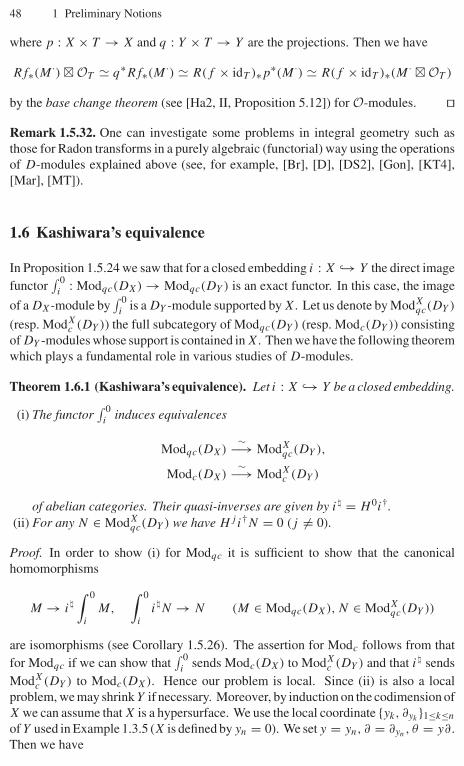
48 1 Preliminary Notions
where p : X × T → X and q : Y × T → Y are the projections. Then we have
Rf∗(M ·) � OT � q∗Rf∗(M ·) � R(f × idT )∗p∗(M ·) � R(f × idT )∗(M · � OT )
by the base change theorem (see [Ha2, II, Proposition 5.12]) for O-modules. ��Remark 1.5.32. One can investigate some problems in integral geometry such asthose for Radon transforms in a purely algebraic (functorial) way using the operationsof D-modules explained above (see, for example, [Br], [D], [DS2], [Gon], [KT4],[Mar], [MT]).
1.6 Kashiwara’s equivalence
In Proposition 1.5.24 we saw that for a closed embedding i : X ↪→ Y the direct imagefunctor
∫ 0i
: Modqc(DX) → Modqc(DY ) is an exact functor. In this case, the image
of a DX-module by∫ 0
iis a DY -module supported by X. Let us denote by ModX
qc(DY )
(resp. ModXc (DY )) the full subcategory of Modqc(DY ) (resp. Modc(DY )) consisting
of DY -modules whose support is contained in X. Then we have the following theoremwhich plays a fundamental role in various studies of D-modules.
Theorem 1.6.1 (Kashiwara’s equivalence). Let i : X ↪→ Y be a closed embedding.
(i) The functor∫ 0
iinduces equivalences
Modqc(DX)∼−→ ModX
qc(DY ),
Modc(DX)∼−→ ModX
c (DY )
of abelian categories. Their quasi-inverses are given by i� = H 0i†.(ii) For any N ∈ ModX
qc(DY ) we have Hj i†N = 0 (j = 0).
Proof. In order to show (i) for Modqc it is sufficient to show that the canonicalhomomorphisms
M → i�
∫ 0
i
M,
∫ 0
i
i�N → N (M ∈ Modqc(DX), N ∈ ModXqc(DY ))
are isomorphisms (see Corollary 1.5.26). The assertion for Modc follows from thatfor Modqc if we can show that
∫ 0i
sends Modc(DX) to ModXc (DY ) and that i� sends
ModXc (DY ) to Modc(DX). Hence our problem is local. Since (ii) is also a local
problem, we may shrink Y if necessary. Moreover, by induction on the codimension ofX we can assume that X is a hypersurface. We use the local coordinate {yk, ∂yk
}1≤k≤n
of Y used in Example 1.3.5 (X is defined by yn = 0). We set y = yn, ∂ = ∂yn, θ = y∂ .Then we have
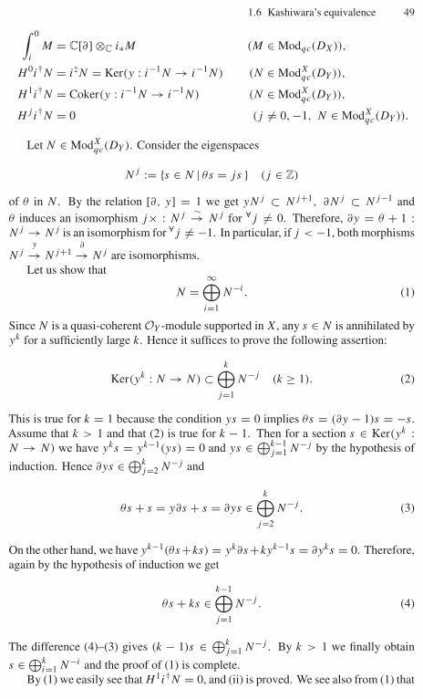
1.6 Kashiwara’s equivalence 49∫ 0
i
M = C[∂] ⊗C i∗M (M ∈ Modqc(DX)),
H 0i†N = i�N = Ker(y : i−1N → i−1N) (N ∈ ModXqc(DY )),
H 1i†N = Coker(y : i−1N → i−1N) (N ∈ ModXqc(DY )),
Hj i†N = 0 (j = 0, −1, N ∈ ModXqc(DY )).
Let N ∈ ModXqc(DY ). Consider the eigenspaces
Nj := {s ∈ N | θs = js } (j ∈ Z)
of θ in N . By the relation [∂, y] = 1 we get yNj ⊂ Nj+1, ∂Nj ⊂ Nj−1 andθ induces an isomorphism j× : Nj ∼→ Nj for ∀j = 0. Therefore, ∂y = θ + 1 :Nj → Nj is an isomorphism for ∀j = −1. In particular, if j < −1, both morphisms
Njy
→ Nj+1∂
→ Nj are isomorphisms.Let us show that
N =∞⊕
i=1
N−i . (1)
Since N is a quasi-coherent OY -module supported in X, any s ∈ N is annihilated byyk for a sufficiently large k. Hence it suffices to prove the following assertion:
Ker(yk : N → N) ⊂k⊕
j=1
N−j (k ≥ 1). (2)
This is true for k = 1 because the condition ys = 0 implies θs = (∂y − 1)s = −s.Assume that k > 1 and that (2) is true for k − 1. Then for a section s ∈ Ker(yk :N → N) we have yks = yk−1(ys) = 0 and ys ∈ ⊕k−1
j=1 N−j by the hypothesis of
induction. Hence ∂ys ∈ ⊕kj=2 N−j and
θs + s = y∂s + s = ∂ys ∈k⊕
j=2
N−j . (3)
On the other hand, we have yk−1(θs +ks) = yk∂s +kyk−1s = ∂yks = 0. Therefore,again by the hypothesis of induction we get
θs + ks ∈k−1⊕j=1
N−j . (4)
The difference (4)–(3) gives (k − 1)s ∈ ⊕kj=1 N−j . By k > 1 we finally obtain
s ∈ ⊕ki=1 N−i and the proof of (1) is complete.
By (1) we easily see that H 1i†N = 0, and (ii) is proved. We see also from (1) that
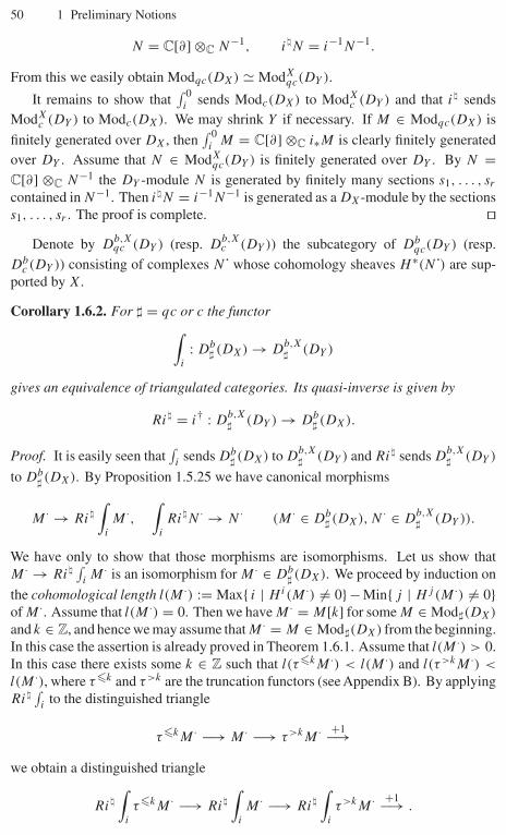
50 1 Preliminary Notions
N = C[∂] ⊗C N−1, i�N = i−1N−1.
From this we easily obtain Modqc(DX) � ModXqc(DY ).
It remains to show that∫ 0
isends Modc(DX) to ModX
c (DY ) and that i� sendsModX
c (DY ) to Modc(DX). We may shrink Y if necessary. If M ∈ Modqc(DX) is
finitely generated over DX, then∫ 0
iM = C[∂] ⊗C i∗M is clearly finitely generated
over DY . Assume that N ∈ ModXqc(DY ) is finitely generated over DY . By N =
C[∂] ⊗C N−1 the DY -module N is generated by finitely many sections s1, . . . , sr
contained in N−1. Then i�N = i−1N−1 is generated as a DX-module by the sectionss1, . . . , sr . The proof is complete. ��
Denote by Db,Xqc (DY ) (resp. D
b,Xc (DY )) the subcategory of Db
qc(DY ) (resp.Db
c (DY )) consisting of complexes N˙ whose cohomology sheaves H ∗(N˙) are sup-ported by X.
Corollary 1.6.2. For � = qc or c the functor∫i
: Db� (DX) → D
b,X� (DY )
gives an equivalence of triangulated categories. Its quasi-inverse is given by
Ri� = i† : Db,X� (DY ) → Db
� (DX).
Proof. It is easily seen that∫
isends Db
� (DX) to Db,X� (DY ) and Ri� sends D
b,X� (DY )
to Db� (DX). By Proposition 1.5.25 we have canonical morphisms
M · → Ri�
∫i
M ·,∫
i
Ri�N · → N · (M · ∈ Db� (DX), N · ∈ D
b,X� (DY )).
We have only to show that those morphisms are isomorphisms. Let us show thatM · → Ri�
∫iM · is an isomorphism for M · ∈ Db
� (DX). We proceed by induction on
the cohomological length l(M ·) := Max{ i | Hi(M ·) = 0}− Min{ j | Hj (M ·) = 0}of M ·. Assume that l(M ·) = 0. Then we have M · = M[k] for some M ∈ Mod�(DX)
and k ∈ Z, and hence we may assume that M · = M ∈ Mod�(DX) from the beginning.In this case the assertion is already proved in Theorem 1.6.1. Assume that l(M ·) > 0.In this case there exists some k ∈ Z such that l(τ�kM ·) < l(M ·) and l(τ>kM ·) <
l(M ·), where τ�k and τ>k are the truncation functors (see Appendix B). By applyingRi�
∫i
to the distinguished triangle
τ�kM · −→ M · −→ τ>kM · +1−→we obtain a distinguished triangle
Ri�
∫i
τ�kM · −→ Ri�
∫i
M · −→ Ri�
∫i
τ>kM · +1−→ .
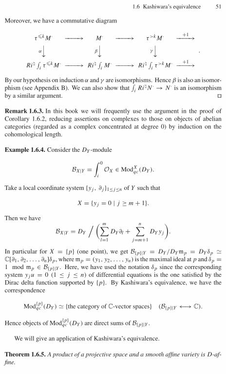
1.6 Kashiwara’s equivalence 51
Moreover, we have a commutative diagram
τ�kM · −−−−→ M · −−−−→ τ>kM · +1−−−−→α
⏐⏐ β
⏐⏐ γ
⏐⏐Ri�
∫iτ�kM · −−−−→ Ri�
∫iM · −−−−→ Ri�
∫iτ>kM · +1−−−−→
.
By our hypothesis on induction α and γ are isomorphisms. Hence β is also an isomor-phism (see Appendix B). We can also show that
∫iRi�N · → N · is an isomorphism
by a similar argument. ��
Remark 1.6.3. In this book we will frequently use the argument in the proof ofCorollary 1.6.2, reducing assertions on complexes to those on objects of abeliancategories (regarded as a complex concentrated at degree 0) by induction on thecohomological length.
Example 1.6.4. Consider the DY -module
BX|Y =∫ 0
i
OX ∈ ModXqc(DY ).
Take a local coordinate system {yj , ∂j }1≤j≤n of Y such that
X = {yj = 0 | j ≥ m + 1}.
Then we have
BX|Y = DY
/ ( m∑l=1
DY ∂l +n∑
j=m+1
DY yj
).
In particular for X = {p} (one point), we get B{p}|Y = DY /DY mp = DY δp �C[∂1, ∂2, . . . , ∂n]δp, where mp = (y1, y2, . . . , yn) is the maximal ideal at p and δp =1 mod mp ∈ B{p}|Y . Here, we have used the notation δp since the correspondingsystem yj u = 0 (1 ≤ j ≤ n) of differential equations is the one satisfied by theDirac delta function supported by {p}. By Kashiwara’s equivalence, we have thecorrespondence
Mod{p}qc (DY ) � {the category of C-vector spaces} (B{p}|Y ←→ C).
Hence objects of Mod{p}qc (DY ) are direct sums of B{p}|Y .
We will give an application of Kashiwara’s equivalence.
Theorem 1.6.5. A product of a projective space and a smooth affine variety is D-af-fine.
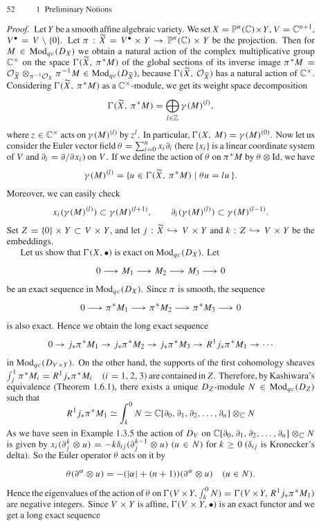
52 1 Preliminary Notions
Proof. Let Y be a smooth affine algebraic variety. We set X = Pn(C)×Y , V = Cn+1,V • = V \ {0}. Let π : X = V • × Y → Pn(C) × Y be the projection. Then forM ∈ Modqc(DX) we obtain a natural action of the complex multiplicative groupC× on the space �(X, π∗M) of the global sections of its inverse image π∗M =OX ⊗π−1OX
π−1M ∈ Modqc(DX), because �(X, OX) has a natural action of C×.Considering �(X, π∗M) as a C×-module, we get its weight space decomposition
�(X, π∗M) =⊕l∈Z
γ (M)(l),
where z ∈ C× acts on γ (M)(l) by zl . In particular, �(X, M) = γ (M)(0). Now let usconsider the Euler vector field θ = ∑n
i=0 xi∂i (here {xi} is a linear coordinate systemof V and ∂i = ∂/∂xi) on V . If we define the action of θ on π∗M by θ ⊗ Id, we have
γ (M)(l) = {u ∈ �(X, π∗M) | θu = lu }.Moreover, we can easily check
xi(γ (M)(l)) ⊂ γ (M)(l+1), ∂i(γ (M)(l)) ⊂ γ (M)(l−1).
Set Z = {0} × Y ⊂ V × Y , and let j : X ↪→ V × Y and k : Z ↪→ V × Y be theembeddings.
Let us show that �(X, •) is exact on Modqc(DX). Let
0 −→ M1 −→ M2 −→ M3 −→ 0
be an exact sequence in Modqc(DX). Since π is smooth, the sequence
0 −→ π∗M1 −→ π∗M2 −→ π∗M3 −→ 0
is also exact. Hence we obtain the long exact sequence
0 → j∗π∗M1 → j∗π∗M2 → j∗π∗M3 → R1j∗π∗M1 → · · ·in Modqc(DV ×Y ). On the other hand, the supports of the first cohomology sheaves∫ 1
jπ∗Mi = R1j∗π∗Mi (i = 1, 2, 3) are contained in Z. Therefore, by Kashiwara’s
equivalence (Theorem 1.6.1), there exists a unique DZ-module N ∈ Modqc(DZ)
such that
R1j∗π∗M1 �∫ 0
k
N � C[∂0, ∂1, ∂2, . . . , ∂n] ⊗C N
As we have seen in Example 1.3.5 the action of DV on C[∂0, ∂1, ∂2, . . . , ∂n] ⊗C N
is given by xi(∂kj ⊗ u) = −kδij (∂k−1
j ⊗ u) (u ∈ N) for k ≥ 0 (δij is Kronecker’sdelta). So the Euler operator θ acts on it by
θ(∂α ⊗ u) = −(|α| + (n + 1))(∂α ⊗ u) (u ∈ N).
Hence the eigenvalues of the action of θ on �(V ×Y,∫ 0
kN) = �(V ×Y, R1j∗π∗M1)
are negative integers. Since V × Y is affine, �(V × Y, •) is an exact functor and weget a long exact sequence
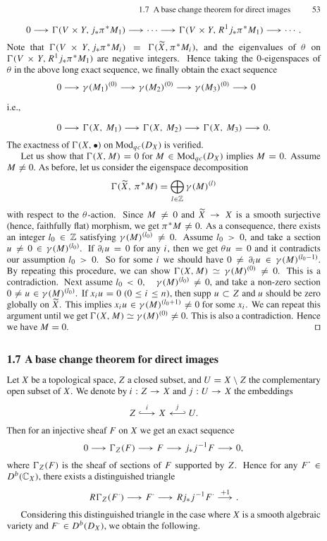
1.7 A base change theorem for direct images 53
0 −→ �(V × Y, j∗π∗M1) −→ · · · −→ �(V × Y, R1j∗π∗M1) −→ · · · .
Note that �(V × Y, j∗π∗Mi) = �(X, π∗Mi), and the eigenvalues of θ on�(V × Y, R1j∗π∗M1) are negative integers. Hence taking the 0-eigenspaces ofθ in the above long exact sequence, we finally obtain the exact sequence
0 −→ γ (M1)(0) −→ γ (M2)(0) −→ γ (M3)(0) −→ 0
i.e.,
0 −→ �(X, M1) −→ �(X, M2) −→ �(X, M3) −→ 0.
The exactness of �(X, •) on Modqc(DX) is verified.Let us show that �(X, M) = 0 for M ∈ Modqc(DX) implies M = 0. Assume
M = 0. As before, let us consider the eigenspace decomposition
�(X, π∗M) =⊕l∈Z
γ (M)(l)
with respect to the θ -action. Since M = 0 and X → X is a smooth surjective(hence, faithfully flat) morphism, we get π∗M = 0. As a consequence, there existsan integer l0 ∈ Z satisfying γ (M)(l0) = 0. Assume l0 > 0, and take a sectionu = 0 ∈ γ (M)(l0). If ∂iu = 0 for any i, then we get θu = 0 and it contradictsour assumption l0 > 0. So for some i we should have 0 = ∂iu ∈ γ (M)(l0−1).By repeating this procedure, we can show �(X, M) � γ (M)(0) = 0. This is acontradiction. Next assume l0 < 0, γ (M)(l0) = 0, and take a non-zero section0 = u ∈ γ (M)(l0). If xiu = 0 (0 ≤ i ≤ n), then supp u ⊂ Z and u should be zeroglobally on X. This implies xiu ∈ γ (M)(l0+1) = 0 for some xi . We can repeat thisargument until we get �(X, M) � γ (M)(0) = 0. This is also a contradiction. Hencewe have M = 0. ��
1.7 A base change theorem for direct images
Let X be a topological space, Z a closed subset, and U = X \ Z the complementaryopen subset of X. We denote by i : Z → X and j : U → X the embeddings
Zi
↪−→ Xj←−↩ U.
Then for an injective sheaf F on X we get an exact sequence
0 −→ �Z(F ) −→ F −→ j∗j−1F −→ 0,
where �Z(F ) is the sheaf of sections of F supported by Z. Hence for any F˙ ∈Db(CX), there exists a distinguished triangle
R�Z(F ·) −→ F · −→ Rj∗j−1F · +1−→ .
Considering this distinguished triangle in the case where X is a smooth algebraicvariety and F · ∈ Db(DX), we obtain the following.
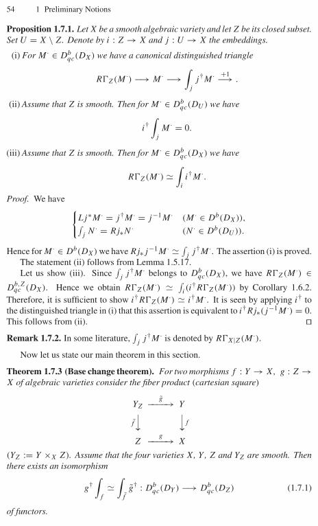
54 1 Preliminary Notions
Proposition 1.7.1. Let X be a smooth algebraic variety and let Z be its closed subset.Set U = X \ Z. Denote by i : Z → X and j : U → X the embeddings.
(i) For M · ∈ Dbqc(DX) we have a canonical distinguished triangle
R�Z(M ·) −→ M · −→∫
j
j†M · +1−→ .
(ii) Assume that Z is smooth. Then for M · ∈ Dbqc(DU ) we have
i†∫
j
M · = 0.
(iii) Assume that Z is smooth. Then for M · ∈ Dbqc(DX) we have
R�Z(M ·) �∫
i
i†M ·.
Proof. We have {Lj∗M · = j†M · = j−1M · (M · ∈ Db(DX)),∫
jN · = Rj∗N · (N · ∈ Db(DU )).
Hence for M · ∈ Db(DX) we have Rj∗j−1M · � ∫j
j†M ·. The assertion (i) is proved.The statement (ii) follows from Lemma 1.5.17.Let us show (iii). Since
∫j
j†M · belongs to Dbqc(DX), we have R�Z(M ·) ∈
Db,Zqc (DX). Hence we obtain R�Z(M ·) � ∫
i(i†R�Z(M ·)) by Corollary 1.6.2.
Therefore, it is sufficient to show i†R�Z(M ·) � i†M ·. It is seen by applying i† tothe distinguished triangle in (i) that this assertion is equivalent to i†Rj∗(j−1M ·) = 0.This follows from (ii). ��Remark 1.7.2. In some literature,
∫j
j†M · is denoted by R�X|Z(M ·).
Now let us state our main theorem in this section.
Theorem 1.7.3 (Base change theorem). For two morphisms f : Y → X, g : Z →X of algebraic varieties consider the fiber product (cartesian square)
YZg−−−−→ Y
f
⏐⏐ ⏐⏐f
Zg−−−−→ X
(YZ := Y ×X Z). Assume that the four varieties X, Y , Z and YZ are smooth. Thenthere exists an isomorphism
g†∫
f
�∫
f
g† : Dbqc(DY ) −→ Db
qc(DZ) (1.7.1)
of functors.

1.7 A base change theorem for direct images 55
Proof. We can decompose the morphism g : Z → X as g : Z ↪→ Z × X → X,where Z ↪→ Z × X is the graph embedding of g and Z × X → X is the projection.Hence by Proposition 1.5.11 it is enough to prove the theorem in the case where g isa projection or a closed embedding (such that YZ is smooth).
(i) Let g = prX : Z = T × X → X be a projection (T is smooth). In this casewe have a cartesian square
T × Yg−−−−→ Y
f
⏐⏐ ⏐⏐f
T × Xg−−−−→ X,
where g = prY , f = idT × f . Then for M · ∈ Dbqc(DY ) we have∫
f
g†M ·[− dim T ] �∫
idT ×f
(OT � M ·) � OT �∫
f
M · � g†∫
f
M ·[− dim T ].
(ii) Let i = g : Z ↪→ X be a closed embedding such that YZ is smooth. Then wehave the two cartesian squares
YZ =f −1(Z)i−−−−→ Y
j←−−−− V = f −1(U)
f
⏐⏐ f
⏐⏐ h
⏐⏐Z
i−−−−→ Xj←−−−− U = X \ Z.
By Kashiwara’s equivalence we have i†∫
i� Id and hence∫
f
i† � i†∫
i
∫f
i† � i†∫
f
∫i
i†.
Hence the canonical morphism∫
ii† → Id (see Proposition 1.7.1) yields the morphism∫
fi† → i†
∫f
. We need to show
i†∫
f
∫i
i†M · � i†∫
f
M ·
for M · ∈ Dqc(DY ). Applying i†∫
fto the distinguished triangle∫
i
i†M · −→ M · −→∫
j
j†M · +1−→
we see that our assertion is equivalent to i†∫
f
∫j
j†M · = 0. By i†∫
f
∫j
j†M · =i†∫
j
∫h
j†M · this follows from Proposition 1.7.1 (ii). ��Corollary 1.7.4. We keep the notation of Theorem 1.7.3. If g(Z) ∩ f (Y ) = ∅, thenwe have
∫f
g† = 0.
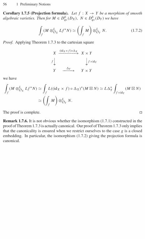
56 1 Preliminary Notions
Corollary 1.7.5 (Projection formula). Let f : X → Y be a morphism of smoothalgebraic varieties. Then for M ∈ Db
qc(DX), N ∈ Dbqc(DY ) we have∫
f
(M ⊗LOX
Lf ∗N) �(∫
f
M
)⊗L
OYN. (1.7.2)
Proof. Applying Theorem 1.7.3 to the cartesian square
X(idX×f )◦�X−−−−−−−→ X × Y
f
⏐⏐ ⏐⏐f ×idY
Y�Y−−−−→ Y × Y
we have∫f
(M ⊗LOX
Lf ∗N) �∫
f
L((idX × f ) ◦ �X)∗(M � N) � L�∗Y
∫f ×idY
(M � N)
�(∫
f
M
)⊗L
OYN.
The proof is complete. ��Remark 1.7.6. It is not obvious whether the isomorphism (1.7.1) constructed in theproof of Theorem 1.7.3 is actually canonical. Our proof of Theorem 1.7.3 only impliesthat the canonicality is ensured when we restrict ourselves to the case g is a closedembedding. In particular, the isomorphism (1.7.2) giving the projection formula iscanonical.
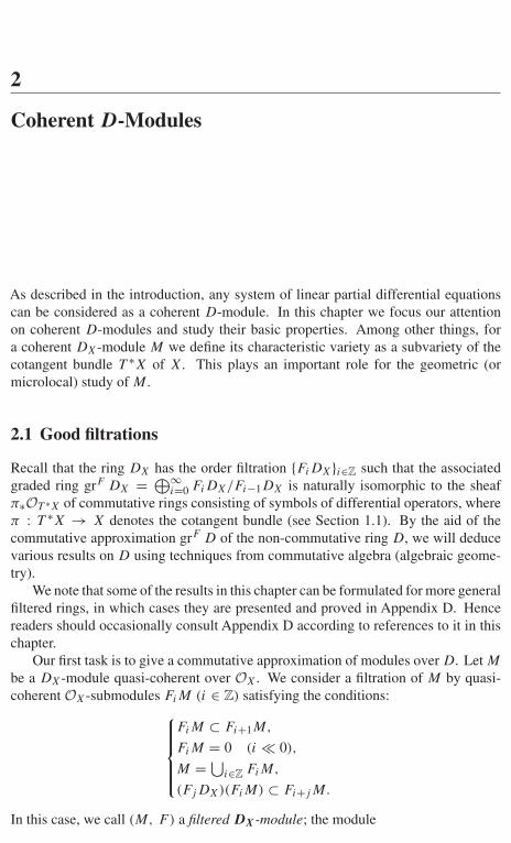
2
Coherent D-Modules
As described in the introduction, any system of linear partial differential equationscan be considered as a coherent D-module. In this chapter we focus our attentionon coherent D-modules and study their basic properties. Among other things, fora coherent DX-module M we define its characteristic variety as a subvariety of thecotangent bundle T ∗X of X. This plays an important role for the geometric (ormicrolocal) study of M .
2.1 Good filtrations
Recall that the ring DX has the order filtration {FiDX}i∈Z such that the associatedgraded ring grF DX = ⊕∞
i=0 FiDX/Fi−1DX is naturally isomorphic to the sheafπ∗OT ∗X of commutative rings consisting of symbols of differential operators, whereπ : T ∗X → X denotes the cotangent bundle (see Section 1.1). By the aid of thecommutative approximation grF D of the non-commutative ring D, we will deducevarious results on D using techniques from commutative algebra (algebraic geome-try).
We note that some of the results in this chapter can be formulated for more generalfiltered rings, in which cases they are presented and proved in Appendix D. Hencereaders should occasionally consult Appendix D according to references to it in thischapter.
Our first task is to give a commutative approximation of modules over D. Let M
be a DX-module quasi-coherent over OX. We consider a filtration of M by quasi-coherent OX-submodules FiM (i ∈ Z) satisfying the conditions:⎧⎪⎪⎪⎨⎪⎪⎪⎩
FiM ⊂ Fi+1M,
FiM = 0 (i # 0),
M = ⋃i∈Z FiM,
(Fj DX)(FiM) ⊂ Fi+j M.
In this case, we call (M, F ) a filtered DX-module; the module
58 2 Coherent D-Modules
grF M :=⊕i∈Z
FiM/Fi−1M
obtained by F is a graded module over grF DX = π∗OT ∗X. This module is clearlyquasi-coherent over OX.
Proposition 2.1.1. Let (M, F ) be a filtered DX-module. Then the following condi-tions are equivalent to each other:
(i) grF M is coherent over π∗OT ∗X.(ii) FiM is coherent over OX for each i, and there exists i0 � 0 satisfying
(Fj DX)(FiM) = Fj+iM (j ≥ 0, i ≥ i0).
(iii) There exist locally a surjective DX-linear morphism � : D⊕mX → M and integers
nj (j = 1, 2, . . . , m) such that
�(Fi−n1DX ⊕ Fi−n2DX ⊕ · · · ⊕ Fi−nmDX) = FiM (i ∈ Z).
Proof. By Proposition D.1.1 the conditions (i) and (iii) are equivalent. It is easilychecked that (iii) holds if and only if FiM is coherent over OX for each i and onecan find i0 as in (ii) locally on X. Then the global existence of i0 follows from thissince X is quasi-compact. ��
Definition 2.1.2. Let (M, F ) be a filtered DX-module. We say that F is a goodfiltration of M if the equivalent conditions in Proposition 2.1.1 are satisfied.
Theorem 2.1.3.
(i) Any coherent DX-module admits a (globally defined) good filtration. Conversely,a DX-module endowed with a good filtration is coherent.
(ii) Let F, F ′ be two filtrations of a DX-module M and assume that F is good. Thenthere exists i0 � 0 such that
FiM ⊂ F ′i+i0
M (i ∈ Z).
If, moreover, F ′ is also a good filtration, there exists i0 � 0 such that
F ′i−i0
M ⊂ FiM ⊂ F ′i+i0
M (i ∈ Z).
Proof. (i) By Corollary D.1.2 an object of Modqc(DX) is coherent if and only if itadmits a good filtration locally on X. Hence it is sufficient to show that any coherentDX-module M admits a global good filtration. By Corollary 1.4.17 (i), M is generatedby a globally defined coherent OX-submodule M0. If we set FiM = (FiDX)M0(i ∈ N), then this is a global good filtration of M . The statement (ii) follows fromProposition D.1.3. ��

2.2 Characteristic varieties (singular supports) 59
2.2 Characteristic varieties (singular supports)
Let M be a coherent DX-module and choose a good filtration F on it (Theorem 2.1.3).Let π : T ∗X → X be the cotangent bundle of X. Since we have grF DX � π∗OT ∗X,the graded module grF M of M obtained by F is a coherent module over π∗OT ∗X byProposition 2.1.1. We call the support of the coherent OT ∗X-module
grF M := OT ∗X ⊗π−1π∗OT ∗Xπ−1(grF M)
the characteristic variety of M and denote it by Ch(M) (it is sometimes called thesingular support of M and denoted by SS(M)). As we see below Ch(M) does
not depend on the choice of a good filtration F on M . Since grF M is a gradedmodule over the graded ring OT ∗X, Ch(M) is a closed conic (i.e., stable by the scalarmultiplication of complex numbers on the fibers) algebraic subset in T ∗X.
Let U be an affine open subset of X. Then T ∗U is an affine open subset of T ∗X
with coordinate algebra grF DU (U), and Ch(M)∩T ∗U coincides with the support ofthe coherent OT ∗U -module associated to the finitely generated grF DU (U)-modulegrF M(U). Hence in the notation of Section D.3 we have
Ch(M) ∩ T ∗U = {p ∈ T ∗U | f (p) = 0 (∀f ∈ JM(U))},and its decomposition into irreducible components is given by
Ch(M) ∩ T ∗U =⋃
p∈SS0(M(U))
{p ∈ T ∗U | f (p) = 0 (∀f ∈ p)}.
By Lemmas D.3.1 and D.3.3 we have the following.
Theorem 2.2.1.(i) Let M be a coherent DX-module. Then the set Ch(M) does not depend on the
choice of a good filtration F .(ii) For a short exact sequence
0 −→ M −→ N −→ L −→ 0
of coherent DX-modules, we have
Ch(N) = Ch(M) ∪ Ch(L).
By the above theorem, the characteristic variety is a geometric invariant of acoherent D-module.
From now on we introduce the notion of the characteristic cycle, which is a finerinvariant of a coherent D-module (obtained by taking the multiplicities into account).
Let V be a smooth algebraic variety and assume that we are given a coherentOV -module G. Then we can define an algebraic cycle Cyc G associated to G asfollows. Denote by I (supp G) the set of the irreducible components of the supportof G. Let C ∈ I (supp G). Take an affine open subset U of V such that C ∩ U = C,
60 2 Coherent D-Modules
and denote the defining ideal of C ∩ U by pC ⊂ OU (U). Then we obtain a local ringOU (U)pC
with maximal ideal pCOU (U)pCand an OU (U)pC
-module G(U)pC. Note
that OU (U)pCand G(U)pC
do not depend on the choice of U (in scheme-theoreticallanguage they are the stalks of OV and G at the generic point of C). By a standardfact in commutative algebra G(U)pC
is an artinian OU (U)pC-module, and its length
mC(G) is defined. We call it the multiplicity of G along C. For an irreduciblesubvariety C of V with C ⊂ supp G we set mC(G) = 0. We call the formal sum
Cyc G :=∑
C∈I (supp G)
mC(G)C
the associated cycle of G.Let M be a coherent DX-module. By choosing a good filtration F of M we can
consider a coherent OT ∗X-module grF M . By Lemma D.3.1 the cycle Cyc(grF M)
does not depend on the choice of a good filtration F .
Definition 2.2.2. For a coherent DX-module M we define the characteristic cycle ofM by
CC(M) := Cyc(grF M) =∑
C∈I (Ch(M))
mC(grF M)C,
where F is a good filtration of M . For d ∈ N we denote its degree d part by
CCd(M) :=∑
C∈I (Ch(M))dim C=d
mC(grF M)C.
By Lemma D.3.3 we have the following.
Theorem 2.2.3. Let0 −→ M −→ N −→ L −→ 0
be an exact sequence of coherent DX-modules. Then for any irreducible subvarietyC of T ∗X such that C ∈ I (Ch(N)) we have
mC(grF N) = mC(grF M) + mC(grF L).
In particular, for d = dim Ch(N) we have
CCd(N) = CCd(M) + CCd(L).
Example 2.2.4. Let M be an integrable connection of rank r > 0. Set FiM = 0(i < 0), FiM = M (i ≥ 0). Then F defines a good filtration on M and grF M � M �Or
X holds locally. Moreover, since �X ⊂ Annπ∗OT ∗X(grF M), we get Ch(M) =
T ∗XX = s(X) � X (s : x �→ (x, 0), the zero-section of T ∗X) and CC(M) = r T ∗
XX.
Conversely, integrable connections are characterized by their characteristic vari-eties as follows.
2.2 Characteristic varieties (singular supports) 61
Proposition 2.2.5. For a non-zero coherent DX-module M the following three con-ditions are equivalent:
(i) M is an integrable connection.(ii) M is coherent over OX.
(iii) Ch(M) = T ∗XX � X (the zero-section of T ∗X).
Proof. Since the equivalence (i) ⇔ (ii) is already proved in Theorem 1.4.10 and (i)⇒ (iii) is explained in Example 2.2.4, it remains to prove the part (iii) ⇒ (ii). Sincethe problem is local, we may assume that X is an affine algebraic variety with alocal coordinate system {xi, ∂i}1≤i≤n. Then we have T ∗X = X × Cn. Assume thatCh(M) = T ∗
XX. This means that for a good filtration F of M we have
√AnnOX[ξ1,...,ξn](grF M) =
n∑i=1
OX[ξ ] ξi .
Here we denote by ξi the principal symbol of ∂i , and we identify π∗OT ∗X withOX[ξ1, . . . , ξn]. Now let us set I = ∑n
i=1 OX[ξ ] ξi . Since the ideal I is noetherian,we have
Im0 ⊂ AnnOX[ξ1,...,ξn](grF M)
for m0 � 0. Since the set {ξα | |α| = m0} generates the ideal Im0 , we have
∂αFj M ⊂ Fj+m0−1M (|α| = m0).
On the other hand, since F is a good filtration, we have FiDX Fj M = Fi+j M
(j � 0). It follows that
Fm0+j M = (Fm0DX)(Fj M)
=∑
|α|≤m0
OX∂αFj M
⊂ Fj+m0−1M (j � 0).
This means Fj+1M = Fj M = M (j � 0). Since each Fj M is coherent over OX,M is also OX-coherent. ��Exercise 2.2.6. For a coherent DX-module M = DXu � DX/I (I = AnnDX
u)consider the good filtration FiM = (FiDX)u. If we define a filtration on I byFiI := FiDX ∩ I , we have grF M � grF DX/ grF I . In this case, the graded idealgrF I := ∑
i≥0 FiI/Fi−1I is generated by the principal symbols σ(P ) of P ∈ I .Therefore, for an arbitrary chosen set {σ(Pi) | 1 ≤ i ≤ m } of generators of grF I , wehave I = ∑m
i=1 DXPi and
Ch(M) = { (x, ξ) ∈ T ∗X | σ(Pi)(x, ξ) = 0, 1 ≤ i ≤ m }.However, for a set {Qi} of generators of I , the equality

62 2 Coherent D-Modules
Ch(M) = { (x, ξ) | σ(Qi)(x, ξ) = 0, 1 ≤ i ≤ m}does not always hold. In general, we have only the inclusion
Ch(M) ⊂ { (x, ξ) | σ(Qi)(x, ξ) = 0, 1 ≤ i ≤ m}.Find an example so that this inclusion is strict.
Remark 2.2.7. In general, it is not easy to compute the characteristic variety of a givencoherent D-module as seen from Exercise 2.2.6. However, thanks to recent advancesin the theory of computational algebraic analysis we now have an effective algorithmto compute their characteristic varieties. Moreover, we can now compute most of theoperations of D-modules by computer programs. For example, we refer to [Oa1],[Oa2], [SST], [Ta]. It is also an interesting problem to determine various invariants ofspecial holonomic D-modules introduced in the theory of hypergeometric functionsof several variables (see [AK], [GKZ]).
2.3 Dimensions of characteristic varieties
One of the most fundamental results in the theory of D-modules is the followingresult about the characteristic varieties of coherent D-modules.
Theorem 2.3.1. The characteristic variety of any coherent DX-module is involutivewith respect to the symplectic structure of the cotangent bundle T ∗X.
This result was first established by Sato–Kawai–Kashiwara [SKK] by an analyticmethod. Different proofs were also given by Malgrange [Ma5], Gabber [Ga], andKashiwara–Schapira [KS2]. Here, we only note that in view of Lemma E.2.3 it isa consequence of Gabber’s theorem (Theorem D.3.4), which is a deep result on acertain class of filtered rings (the proof of Theorem D.3.4 is not given in this book).
An important consequence of Theorem 2.3.1 is the following result.
Corollary 2.3.2. Let M be a coherent DX-module. Then for any irreducible compo-nent � of Ch(M) we have dim � ≥ dim X. In particular, we have dim Ch(M) ≥dim X if M = 0.
Remark 2.3.3. Note that Corollary 2.3.2 is weaker than Theorem 2.3.1; however, theweaker statement Corollary 2.3.2 is almost sufficient for arguments in this book. Infact, we will need the stronger statement Theorem 2.3.1 (or rather its analytic counter-part Theorem 4.1.3 below) only in the proof of Kashiwara’s constructibility theoremfor solutions of analytic holonomic D-modules (Theorem 4.6.3 below). Since we willalso present a proof of the corresponding fact for algebraic holonomic D-modulesdue to Beilinson–Bernstein without using Theorem 2.3.1 (see Theorem 4.7.7 below),the readers who are only interested in algebraic D-modules can skip Section 4.6.
In the rest of this section we will give a direct proof of Corollary 2.3.2 followingKashiwara [Kas16].
We first establish the following result.

2.3 Dimensions of characteristic varieties 63
Theorem 2.3.4. For any coherent DX-module M there exists a canonical filtration
0 = C2 dim X+1M ⊂ C2 dim XM ⊂ · · · ⊂ C1M ⊂ C0M = M
of M by coherent DX-modules such that any irreducible component of
Ch(CsM/Cs+1M)
is s-codimensional in T ∗X.
Proof. Let U be an affine open subset of X. We apply the result in Section D.5 to A =DX(U). Then by Lemma D.5.1 and Theorem D.5.3, together with Proposition 1.4.13,we obtain a filtration
0 = C2 dim X+1(M|U ) ⊂ C2 dim X(M|U ) ⊂ · · · ⊂ C0(M|U ) = M|Uof M|U by coherent DU -modules such that any irreducible component ofCh(Cs(M|U )/Cs+1(M|U )) is s-codimensional in T ∗U . We see by the cohomo-logical description of the filtration given in Proposition D.5.2 that it is canonical andglobally defined on X. ��Lemma 2.3.5. Let S be a smooth closed subvariety of X and let M be a coherentDS-module. Set N = ∫ 0
iM , where i : S ↪→ X denotes the embedding. Let ρi :
S ×X T ∗X → T ∗S and let �i : S ×X T ∗X ↪→ T ∗X be natural morphisms inducedby i. Then we have
Ch(N) = �iρ−1i (Ch(M)).
Proof. Note that the problem is local on S. By induction on the codimension of S
one can reduce the problem to the case where S is a hypersurface of X (see Proposi-tion 1.5.21 and Lemma 2.4.1 below). Assume that S is a hypersurface of X definedby x = 0. Take a local coordinate {xi, ∂i}1≤i≤n of X such that x = x1 and set ∂ = ∂1.Then we obtain a local identification N � C[∂] ⊗C i∗M (see Section 1.5). Take agood filtration G of M such that G−1M = 0, and define a filtration F of N by
Fj N =j∑
l=0
∑k≤l
C∂k ⊗ i∗Gj−l (M).
Then F is a good filtration of N satisfying
Fj N/Fj−1N =j⊕
l=0
C∂l ⊗ i∗(Gj−lM/Gj−l−1M).
Hence we have
grF N � C[ξ ] ⊗C grG M � (C[x, ξ ]/C[x, ξ ]x) ⊗C grG M,
where ξ is the principal symbol of ∂ . From this we easily see that
Ch(N) = supp grF N = �iρ−1i (supp grG M = �iρ
−1i (Ch(M)).
The proof is complete. ��
64 2 Coherent D-Modules
Proof of Corollary 2.3.2. By Theorem 2.3.4 we have only to show that
dim Ch(M) ≥ dim X
for any non-zero coherent DX-module M . We prove it by induction on dim X. It istrivial in the case dim X = 0. Assume that dim X > 0. If supp M = X, then we haveCh(M) ⊃ T ∗
XX, and hence dim Ch(M) ≥ dim T ∗XX = dim X. Therefore, we may
assume from the beginning that supp M is a proper closed subset of X. By replacingX with a suitable open subset (if necessary) we may further assume that supp M iscontained in a smooth hypersurface S in X. Let i : S → X be the embedding. ByKashiwara’s equivalence there exists a non-zero coherent DS-module L satisfyingM = ∫ 0
iL. Then by Lemma 2.3.5 we have Ch(M) = �iρ
−1i (Ch(L)) and hence
dim Ch(M) = dim Ch(L) + 1. On the other hand, the hypothesis of inductionimplies dim Ch(L) ≥ dim S = dim X − 1. It follows that dim Ch(M) ≥ dim S + 1= dim X. ��Definition 2.3.6. A coherent DX-module M is called a holonomic DX-module (or aholonomic system, or a maximally overdetermined system) if it satisfies dim Ch(M) �dim X.
By Theorem 2.3.1 characteristic varieties of holonomic D-modules are C×-invariant Lagrangian subset of T ∗X.
Holonomic DX-modules are the coherent DX-modules whose characteristic va-riety has minimal possible dimension dim X. Assume that the dimension of thecharacteristic variety Ch(M) is “small.’’ This means that the ideal defining the cor-responding system of differential equations is “large,’’ and hence the space of thesolutions should be “small.’’ In fact, we will see later that the holonomicity is relatedto the finite dimensionality of the solution space.
Example 2.3.7. Integrable connections are holonomic by Proposition 2.2.5.
Example 2.3.8. The DX-module BY |X for a closed smooth subvariety Y of X isholonomic (see Example 1.6.4). In this case the characteristic variety Ch(BY |X) isthe conormal bundle T ∗
Y X of Y in X.
2.4 Inverse images in the non-characteristic case
We have shown in Proposition 1.5.13 that the inverse image of a coherent D-modulewith respect to a smooth morphism is again coherent; however, the inverse imageswith respect to non-smooth morphisms do not necessarily preserve coherency as wesaw in Example 1.5.10. In this section we will give a sufficient condition on a coherentD-module M so that its inverse image is again coherent.
For a morphism f : X → Y of smooth algebraic varieties there are associatednatural morphisms
T ∗Xρf←−−−−− X ×Y T ∗Y
�f−−−−−→ T ∗Y.
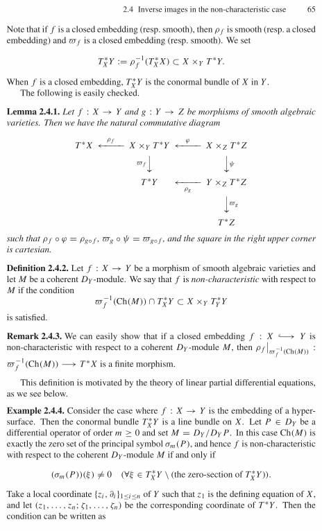
2.4 Inverse images in the non-characteristic case 65
Note that if f is a closed embedding (resp. smooth), then ρf is smooth (resp. a closedembedding) and �f is a closed embedding (resp. smooth). We set
T ∗XY := ρ−1
f (T ∗XX) ⊂ X ×Y T ∗Y.
When f is a closed embedding, T ∗XY is the conormal bundle of X in Y .
The following is easily checked.
Lemma 2.4.1. Let f : X → Y and g : Y → Z be morphisms of smooth algebraicvarieties. Then we have the natural commutative diagram
T ∗Xρf←−−−− X ×Y T ∗Y
ϕ←−−−− X ×Z T ∗Z
�f
⏐⏐ ⏐⏐ψ
T ∗Y ←−−−−ρg
Y ×Z T ∗Z⏐⏐�g
T ∗Z
such that ρf ◦ ϕ = ρg◦f , �g ◦ ψ = �g◦f , and the square in the right upper corneris cartesian.
Definition 2.4.2. Let f : X → Y be a morphism of smooth algebraic varieties andlet M be a coherent DY -module. We say that f is non-characteristic with respect toM if the condition
�−1f (Ch(M)) ∩ T ∗
XY ⊂ X ×Y T ∗Y Y
is satisfied.
Remark 2.4.3. We can easily show that if a closed embedding f : X ↪−→ Y isnon-characteristic with respect to a coherent DY -module M , then ρf
∣∣�−1
f (Ch(M)):
�−1f (Ch(M)) −→ T ∗X is a finite morphism.
This definition is motivated by the theory of linear partial differential equations,as we see below.
Example 2.4.4. Consider the case where f : X → Y is the embedding of a hyper-surface. Then the conormal bundle T ∗
XY is a line bundle on X. Let P ∈ DY be adifferential operator of order m ≥ 0 and set M = DY /DY P . In this case Ch(M) isexactly the zero set of the principal symbol σm(P ), and hence f is non-characteristicwith respect to the coherent DY -module M if and only if
(σm(P ))(ξ) = 0 (∀ξ ∈ T ∗XY \ (the zero-section of T ∗
XY )).
Take a local coordinate {zi, ∂i}1≤i≤n of Y such that z1 is the defining equation of X,and let (z1, . . . , zn; ζ1, . . . , ζn) be the corresponding coordinate of T ∗Y . Then thecondition can be written as
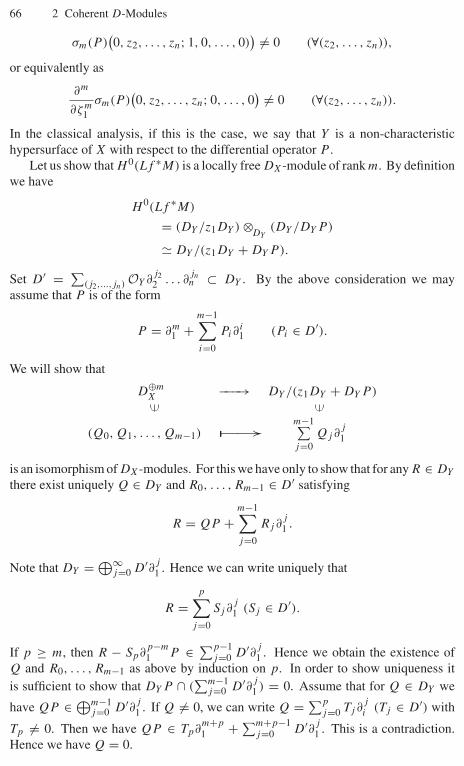
66 2 Coherent D-Modules
σm(P )(0, z2, . . . , zn; 1, 0, . . . , 0)
) = 0 (∀(z2, . . . , zn)),
or equivalently as
∂m
∂ζm1
σm(P )(0, z2, . . . , zn; 0, . . . , 0
) = 0 (∀(z2, . . . , zn)).
In the classical analysis, if this is the case, we say that Y is a non-characteristichypersurface of X with respect to the differential operator P .
Let us show that H 0(Lf ∗M) is a locally free DX-module of rank m. By definitionwe have
H 0(Lf ∗M)
= (DY /z1DY ) ⊗DY
(DY /DY P )
� DY /(z1DY + DY P ).
Set D′ = ∑(j2,...,jn) OY ∂
j22 . . . ∂
jnn ⊂ DY . By the above consideration we may
assume that P is of the form
P = ∂m1 +
m−1∑i=0
Pi∂i1 (Pi ∈ D′).
We will show that
D⊕mX −−−→ DY /(z1DY + DY P )�� ��
(Q0, Q1, . . . , Qm−1) �−→m−1∑j=0
Qj ∂j
1
is an isomorphism of DX-modules. For this we have only to show that for any R ∈ DY
there exist uniquely Q ∈ DY and R0, . . . , Rm−1 ∈ D′ satisfying
R = QP +m−1∑j=0
Rj ∂j
1 .
Note that DY = ⊕∞j=0 D′∂j
1 . Hence we can write uniquely that
R =p∑
j=0
Sj ∂j
1 (Sj ∈ D′).
If p ≥ m, then R − Sp∂p−m
1 P ∈ ∑p−1j=0 D′∂j
1 . Hence we obtain the existence ofQ and R0, . . . , Rm−1 as above by induction on p. In order to show uniqueness itis sufficient to show that DY P ∩ (
∑m−1j=0 D′∂j
1 ) = 0. Assume that for Q ∈ DY we
have QP ∈ ⊕m−1j=0 D′∂j
1 . If Q = 0, we can write Q = ∑p
j=0 Tj ∂ji (Tj ∈ D′) with
Tp = 0. Then we have QP ∈ Tp∂m+p
1 +∑m+p−1j=0 D′∂j
1 . This is a contradiction.Hence we have Q = 0.
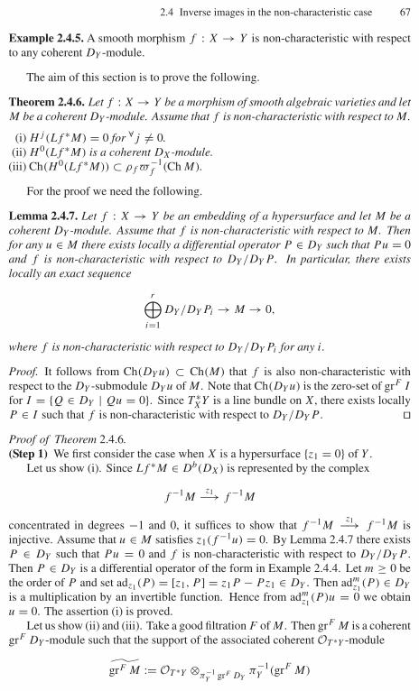
2.4 Inverse images in the non-characteristic case 67
Example 2.4.5. A smooth morphism f : X → Y is non-characteristic with respectto any coherent DY -module.
The aim of this section is to prove the following.
Theorem 2.4.6. Let f : X → Y be a morphism of smooth algebraic varieties and letM be a coherent DY -module. Assume that f is non-characteristic with respect to M .
(i) Hj (Lf ∗M) = 0 for ∀j = 0.(ii) H 0(Lf ∗M) is a coherent DX-module.
(iii) Ch(H 0(Lf ∗M)) ⊂ ρf �−1f (Ch M).
For the proof we need the following.
Lemma 2.4.7. Let f : X → Y be an embedding of a hypersurface and let M be acoherent DY -module. Assume that f is non-characteristic with respect to M . Thenfor any u ∈ M there exists locally a differential operator P ∈ DY such that Pu = 0and f is non-characteristic with respect to DY /DY P . In particular, there existslocally an exact sequence
r⊕i=1
DY /DY Pi → M → 0,
where f is non-characteristic with respect to DY /DY Pi for any i.
Proof. It follows from Ch(DY u) ⊂ Ch(M) that f is also non-characteristic withrespect to the DY -submodule DY u of M . Note that Ch(DY u) is the zero-set of grF I
for I = {Q ∈ DY | Qu = 0}. Since T ∗XY is a line bundle on X, there exists locally
P ∈ I such that f is non-characteristic with respect to DY /DY P . ��Proof of Theorem 2.4.6.(Step 1) We first consider the case when X is a hypersurface {z1 = 0} of Y .
Let us show (i). Since Lf ∗M ∈ Db(DX) is represented by the complex
f −1Mz1−→ f −1M
concentrated in degrees −1 and 0, it suffices to show that f −1Mz1−→ f −1M is
injective. Assume that u ∈ M satisfies z1(f −1u) = 0. By Lemma 2.4.7 there existsP ∈ DY such that Pu = 0 and f is non-characteristic with respect to DY /DY P .Then P ∈ DY is a differential operator of the form in Example 2.4.4. Let m ≥ 0 bethe order of P and set adz1(P ) = [z1, P ] = z1P − Pz1 ∈ DY . Then adm
z1(P ) ∈ DY
is a multiplication by an invertible function. Hence from admz1
(P )u = 0 we obtainu = 0. The assertion (i) is proved.
Let us show (ii) and (iii). Take a good filtration F of M . Then grF M is a coherentgrF DY -module such that the support of the associated coherent OT ∗Y -module
grF M := OT ∗Y ⊗π−1
Y grF DYπ−1
Y (grF M)
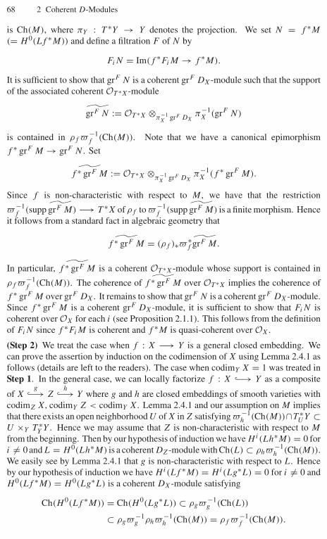
68 2 Coherent D-Modules
is Ch(M), where πY : T ∗Y → Y denotes the projection. We set N = f ∗M
(= H 0(Lf ∗M)) and define a filtration F of N by
FiN = Im(f ∗FiM → f ∗M).
It is sufficient to show that grF N is a coherent grF DX-module such that the supportof the associated coherent OT ∗X-module
grF N := OT ∗X ⊗π−1
X grF DXπ−1
X (grF N)
is contained in ρf �−1f (Ch(M)). Note that we have a canonical epimorphism
f ∗ grF M → grF N . Set
˜f ∗ grF M := OT ∗X ⊗π−1
X grF DXπ−1
X (f ∗ grF M).
Since f is non-characteristic with respect to M , we have that the restriction
�−1f (supp grF M) −→ T ∗X of ρf to �−1
f (supp grF M) is a finite morphism. Henceit follows from a standard fact in algebraic geometry that
˜f ∗ grF M = (ρf )∗� ∗f grF M.
In particular, ˜f ∗ grF M is a coherent OT ∗X-module whose support is contained in
ρf �−1f (Ch(M)). The coherence of ˜f ∗ grF M over OT ∗X implies the coherence of
f ∗ grF M over grF DX. It remains to show that grF N is a coherent grF DX-module.Since f ∗ grF M is a coherent grF DX-module, it is sufficient to show that FiN iscoherent over OX for each i (see Proposition 2.1.1). This follows from the definitionof FiN since f ∗FiM is coherent and f ∗M is quasi-coherent over OX.
(Step 2) We treat the case when f : X −→ Y is a general closed embedding. Wecan prove the assertion by induction on the codimension of X using Lemma 2.4.1 asfollows (details are left to the readers). The case when codimY X = 1 was treated inStep 1. In the general case, we can locally factorize f : X ↪−→ Y as a composite
of Xg
↪−→ Zh
↪−→ Y where g and h are closed embeddings of smooth varieties withcodimZ X, codimY Z < codimY X. Lemma 2.4.1 and our assumption on M impliesthat there exists an open neighborhood U of X in Z satisfying �−1
h (Ch(M))∩T ∗U Y ⊂
U ×Y T ∗Y Y . Hence we may assume that Z is non-characteristic with respect to M
from the beginning. Then by our hypothesis of induction we have Hi(Lh∗M) = 0 fori = 0 and L = H 0(Lh∗M) is a coherent DZ-module with Ch(L) ⊂ ρh�−1
h (Ch(M)).We easily see by Lemma 2.4.1 that g is non-characteristic with respect to L. Henceby our hypothesis of induction we have Hi(Lf ∗M) = Hi(Lg∗L) = 0 for i = 0 andH 0(Lf ∗M) = H 0(Lg∗L) is a coherent DX-module satisfying
Ch(H 0(Lf ∗M)) = Ch(H 0(Lg∗L)) ⊂ ρg�−1g (Ch(L))
⊂ ρg�−1g ρh�−1
h (Ch(M)) = ρf �−1f (Ch(M)).
2.5 Proper direct images 69
(Step 3) If f : X = Y × Z −→ Y is the first projection, then the assertions followseasily from the isomorphism Lf ∗M � M � OZ .
(Step 4) To handle the case of a general morphism f : Y −→ X, we may factorize f
as Yg−→ Y × X
p−→ X, where g is the graph embedding defined by y �→ (y, f (y))
and p is the second projection. Then the result follows from Step 2 and Step 3 byusing Lemma 2.4.1 and the arguments similar to those in Step 2. ��Remark 2.4.8. Under the assumption of Theorem 2.4.6 it is known that we haveactually
Ch(H 0(Lf ∗M)) = ρf �−1f (Ch(M))
(see [Kas8] and [Kas18]).
2.5 Proper direct images
In this section we show the following.
Theorem 2.5.1. Let f : X → Y be a proper morphism. Then for an object M˙ inDb
c (DX) the direct image∫
fM˙ belongs to Db
c (DY ).
Proof. Since we assumed that X and Y are quasi-projective, f is a projective mor-phism. Namely, f is factorized as
Xi
↪−→ Y × Pn p−→ Y
by a closed embedding i (i(x) = (f (x), j (x)), j : X ↪→ Pn) and a projectionp = prY to Y . Hence it is enough to prove our theorem for each case.
(i) The case of closed embeddings i : X ↪→ Y : The problem being local on Y ,we may take a free resolution F · � M · of M · ∈ Db
c (DX) such that each term F j isisomorphic to D
nj
X . Using the exactness of the functor∫
iwe have only to prove the
coherence of∫
iDX over DY . We see by∫
i
DX = i∗(DY←X ⊗DXDX) = i∗(i−1(DY ⊗OY
�⊗−1Y ) ⊗i−1OY
�X)
= DY ⊗OY(�⊗−1
Y ⊗OYi∗�X)
that∫
iDX is locally isomorphic to DY /DY IX where IX ⊂ OY is the defining ideal
of X. In particular, it is coherent.(ii) The case of projections p : X = Y ×Pn → Y : Since the problem is local on Y ,
we may assume that Y is an affine variety. By Theorem 1.6.5 and Proposition 1.4.13there exists a resolution F · � M · of M · in Db
c (DX), where F · is a bounded complexof DX-modules such that each term F j of F · is a direct summand of a free DX-moduleof finite rank. Then it is sufficient to show
∫p
F j ∈ Dbc (DY ) for any j . Assume that
F j is a direct summand of DnX. Then
∫p
F j ∈ Dbqc(DY ) is a direct summand of∫
pDn
X. Hence it is enough to show∫
pDX ∈ Db
c (DY ). By
70 2 Coherent D-Modules
DY←X = �Y×Pn ⊗OY×Pn p∗(DY ⊗OY�⊗−1
Y
) � DY � �Pn ,
we have∫p
DX = Rp∗(DY←X ⊗LDX
DX) � Rp∗(DY � �Pn) � DY ⊗C R�(Pn, �Pn).
Now we recall that the only non-vanishing cohomology group of R�(Pn, �Pn)
is Hn(Pn, �Pn) � C. Therefore, we get that R�(Pn, �Pn) � C[−n] and∫p
DX � DY [−n]. ��Remark 2.5.2. Under the assumption of Theorem 2.5.1 it is known that we have
Ch(∫
f
M ·) ⊂ �f ρ−1f (Ch(M ·)).
As we saw in Lemma 2.3.5 the equality holds in the case where f is a closed embed-ding. The proof for the general case is more involved.
2.6 Duality functors
We first try to find heuristically a candidate for the “dual’’ of a left D-module. LetM be a left DX-module. Then HomDX
(M, DX) is a right DX-module by rightmultiplication of DX on DX. By the side-changing functor ⊗OX
�⊗−1X we obtain a
left DX-module HomDX(M, DX) ⊗OX
�⊗−1X . Since the functor HomDX
(•, DX) isnot exact, it is more natural to consider the complex RHomDX
(M, DX) ⊗OX�⊗−1
X
of left DX-modules. In order to judge which cohomology group of this complexdeserves to be called “dual,’’ let us consider the following example. Let X = C(or an open subset of C) and M = DX/DXP (P = 0). By applying the functorHomDX
(•, DX) to the exact sequence
0 −→ DX×P−→ DX −→ M −→ 0
of left DX-modules we get an exact sequence
0 −→ HomDX(M, DX) −→ DX
P×−→ DX
(note HomDX(DX, DX) � DX). Hence in this case, we have
Ext0DX
(M, DX) = HomDX(M, DX) = Ker(P : DX → DX) = 0
and the only non-vanishing cohomology group is the first one
Ext1DX
(M, DX) � DX/PDX.
The left DX-module obtained by the side changing ⊗ �⊗−1X is isomorphic to
2.6 Duality functors 71
Ext1DX
(M, DX) ⊗OX�⊗−1
X � DX/DXP ∗,
where P ∗ is the formal adjoint of P . From this calculation, we see that Ext1 ismore suited than Ext0 to be called “dual’’ of M . More generally, if n = dim X
and M is a holonomic DX-module, then we can (and will) prove that only theterm Extn
DX(M, DX) survives and the resulting left DX-module Extn
DX(M, DX)⊗OX
�⊗−1X is also holonomic. Hence the correct definition of the dual DM of a holonomic
DX-module M is given by DM = ExtnDX
(M, DX)⊗OX�⊗−1
X . For a non-holonomicDX-module one may have other non-vanishing cohomology groups, and hence theduality functor should be defined as follows for the derived categories.
Definition 2.6.1. We define the duality functor D = DX : D−(DX) → D+(DX)op by
DM · := RHomDX(M ·, DX) ⊗OX
�⊗−1X [dim X]
= RHomDX(M ·, DX ⊗OX
�⊗−1X [dim X]) (M˙ ∈ D−(DX)).
We use the following notation since shifts of complexes by dimensions of varietieswill often appear in the subsequent parts.
Notation 2.6.2. For an algebraic variety X we denote its dimension dim X by dX.
Example 2.6.3. We have
Hk(DDX) ={
DX ⊗OX�⊗−1
X (k = −dX),
0 (k = −dX).
Lemma 2.6.4. Let M be a coherent DX-module. Then for any affine open subset U
of X we have
(ExtiDX
(M, DX))(U) = ExtiDX(U)(M(U), DX(U)).
Proof. Take a resolution P· → M|U of M|U by free DU -modules of finite rank.Since U is affine, P·(U) → M(U) gives a resolution of M(U) by freeDX(U)-modules of finite rank. By definition we have (Exti
DX(M, DX))(U) =
(H i(HomDU(P·, DU )))(U). Set L· = HomDU
(P·, DU ). Since U is affine andL· is a complex of coherent right DU -modules, we have Hi(L·)(U) = Hi(L·(U))
(see Remark 1.4.5 (ii)). Moreover, we have
L·(U) = HomDU(P·, DU ) = HomDX(U)(P·(U), DX(U)).
Here, the first equality is obvious, and the second equality follows easily from thefact that P · is a complex of free DU -modules (or one can use the D-affinity of U ).Therefore, we obtain
(ExtiDX
(M, DX))(U) = Hi(HomDX(U)(P·(U), DX(U)))
= ExtiDX(U)(M(U), DX(U)).
The proof is complete. ��
72 2 Coherent D-Modules
Proposition 2.6.5.(i) The functor D sends Db
c (DX) to Dbc (DX)op.
(ii) D2 � Id on Dbc (DX).
Proof. (i) We may assume that M · = M ∈ Modc(DX). Then we see from (the proofof) Lemma 2.6.4 that Hi(DM) ∈ Modc(DX) for any i. The boundedness of DM
also follows from Lemma 2.6.4 and Proposition 1.4.6 (ii).(ii) We first construct a canonical morphism M · → D2M · for M · ∈ Db(DX).
First note that
D2M · � RHomDopX
(RHomDX(M ·, DX), DX),
where RHomDX(M ·, DX) and DX are regarded as objects of Db(D
opX ) (complexes
of right DX-modules) by the right multiplication of DX on DX, and the left DX-action on the right-hand side is induced from the left multiplication of DX on DX.Set H · = RHomDX
(M ·, DX). By applying H 0(R�(X, •)) to
RHomDX⊗CDopX
(M · ⊗C H ·, DX) � RHomDX(M ·, RHomD
opX
(H ·, DX)),
we obtain
HomDX⊗CDopX
(M · ⊗C H ·, DX) � HomDX(M ·, RHomD
opX
(H ·, DX)).
Hence the canonical morphism M · ⊗C H ·(= M · ⊗C RHomDX(M ·, DX)) → DX in
Db(DX ⊗C DopX ) gives rise to a canonical morphism
M · → RHomDopX
(H ·, DX)(= D2M)
in Db(DX). It remains to show that M · → D2M · is an isomorphism for M · ∈Db
c (DX). Since the question is local, we may assume that X is affine. Then we canreplace M · with DX by Proposition 1.4.13 (see the proof of Theorem 2.5.1). In thiscase the assertion is clear. ��Corollary 2.6.6. D is fully faithful on Db
c (DX).
The following theorem gives an estimate for the dimensions of the characteristicvarieties Ch(H i(DM)) for M ∈ Modc(DX).
Theorem 2.6.7. Let X be a smooth algebraic variety and M a coherent DX-module.
(i) codimT ∗X Ch(ExtiDX
(M, DX) ⊗OX�⊗−1
X ) ≥ i.
(ii) ExtiDX
(M, DX) = 0 (i < codimT ∗X Ch(M)).
This theorem is a consequence of Theorem D.4.3 and Lemma 2.6.4.
Corollary 2.6.8. Let M be a coherent DX-module.
(i) Hi(DM) = 0 unless −(dX − codimT ∗X Ch(M)) ≤ i ≤ 0.
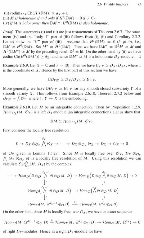
2.6 Duality functors 73
(ii) codimT ∗X Ch(H i(DM)) ≥ dX + i.(iii) M is holonomic if and only if Hi(DM) = 0 (i = 0).(iv) If M is holonomic, then DM � H 0(DM) is also holonomic.
Proof. The statements (i) and (ii) are just restatements of Theorem 2.6.7. The state-ment (iv) and the “only if’’ part of (iii) follows from (i), (ii) and Corollary 2.3.2.Let us show the “if’’ part of (iii). Assume that Hi(DM) = 0 (i = 0), i.e.,DM � H 0(DM). Set M∗ = H 0(DM). Then we have DM∗ = D2M � M andH 0(DM∗) � M by the preceding result D2 = Id. On the other hand by (ii) we havecodim Ch(H 0(DM∗)) ≥ dX, and hence DM∗ � M is a holonomic DX-module. ��Example 2.6.9. Let X = C and Y = {0}. Then we have BY |X � DX/DXx, where x
is the coordinate of X. Hence by the first part of this section we have
DBY |X � DX/DXx � BY |X.
More generally, we have DBY |X � BY |X for any smooth closed subvariety Y of asmooth variety X. This follows from Example 2.6.10, Theorem 2.7.2 below andBY |X = ∫
iOY , where i : Y → X is the embedding.
Example 2.6.10. Let M be an integrable connection. Then by Proposition 1.2.9,HomOX
(M, OX) is a left DX-module (an integrable connection). Let us show that
DM � HomOX(M, OX).
First consider the locally free resolution
0 → DX ⊗OX
dX∧�X → · · · → DX ⊗OX
�X → DX → OX → 0
of OX given in Lemma 1.5.27. Since M is locally free over OX, DX ⊗OX∧·�X ⊗OX
M is a locally free resolution of M . Using this resolution we can
calculate ExtdX
DX(M, DX) by the complex
· · · → HomD
(D ⊗O
dX−1∧� ⊗O M, D
)→ HomD
(D ⊗O
dX∧� ⊗O M, D
)→ 0−→ �
−→ �
HomO(dX−1∧
� ⊗O M, D)
−→ HomO(dX∧
� ⊗O M, D)
−→ �
−→ �HomO
(M, �dX−1 ⊗O D
) δ−→ HomO(M, �dX ⊗O D
).
On the other hand since M is locally free over OX, we have an exact sequence
HomO(M, �dX−1 ⊗O D)δ→ HomO(M, �dX ⊗O D) → HomO(M, �dX) → 0
of right DX-modules. Hence as a right DX-module we have
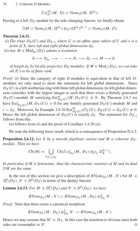
74 2 Coherent D-Modules
ExtdX
D (M, D) � HomO(M, �dX).
Passing to a left DX-module by the side-changing functor, we finally obtain
DM � HomO(M, �dX) ⊗O (�dX)⊗−1 � HomO(M, O).
Theorem 2.6.11.(i) The rings DX(U) and DX,x , where U is an affine open subset of U and x is a
point of X, have left and right global dimensions dX.(ii) Any M ∈ Modqc(DX) admits a resolution
0 −→ PdX−→ · · · −→ P1 −→ P0 −→ M −→ 0
of length dX by locally projective DX-modules. If M ∈ Modc(DX), we can takeall Pi’s to be of finite rank.
Proof. (i) Since the category of right D-modules is equivalent to that of left D-modules we only need to show the statement for left global dimensions. SinceDX(U) is a left noetherian ring with finite left global dimension, its left global dimen-sion coincides with the largest integer m such that there exists a finitely generatedDX(U)-module M satisfying ExtmDX(U)(M, DX(U)) = 0. By Theorem 2.6.7 we
have ExtiDX(U)(M, DX(U)) = 0 for any finitely generated DX(U)-module M and
i > dX. Moreover, by Example 2.6.10 ExtdX
DX(U)(OX(U), DX(U)) = �X(U) = 0.Hence the left global dimension of DX(U) is exactly dX. The statement for DX,x
follows from this.(ii) follows from (i) and the proof of Corollary 1.4.20 (ii).
We note the following basic result, which is a consequence of Proposition D.4.2.
Proposition 2.6.12. Let X be a smooth algebraic variety and M a coherent DX-module. Then we have
Ch(M) =⋃
0≤i≤dX
Ch(ExtiDX
(M, DX) ⊗OX�⊗−1
X ).
In particular, if M is holonomic, then the characteristic varieties of M and its dualDM are the same.
In the rest of this section we give a description of RHomDX(M ·, N ·) for M · ∈
Dbc (DX), N · ∈ Db(DX) in terms of the duality functor.
Lemma 2.6.13. For M · ∈ Dbc (DX) and N · ∈ Db(DX), we have
RHomDX(M ·, N ·) � RHomDX
(M ·, DX) ⊗LDX
N ·.
Proof. Note that there exists a canonical morphism
RHomDX(M ·, DX) ⊗L
DXN · → RHomDX
(M ·, N ·).
Hence we may assume that M · = DX. In this case the assertion is obvious since bothsides are isomorphic to N ·. ��

2.6 Duality functors 75
Proposition 2.6.14. For M · ∈ Dbc (DX), N · ∈ Db(DX) we have isomorphisms
RHomDX(M ·, N ·) � (�X ⊗L
OXDXM ·) ⊗L
DXN ·[−dX]
� �X ⊗LDX
(DXM · ⊗LOX
N ·)[−dX]� RHomDX
(OX, DXM · ⊗LOX
N ·) (2.6.1)
in Db(CX). In particular, we have
RHomDX(OX, N ·) � �X ⊗L
DXN ·[−dX] (2.6.2)
for N · ∈ Db(DX).
Proof. We first show (2.6.2). By Lemma 2.6.13 we may assume that N · = DX. Inthis case we have
RHomDX(OX, DX)
�⎡⎣HomDX
⎛⎝DX ⊗OX
0∧�X, DX
⎞⎠ → · · · → HomDX
⎛⎝DX ⊗OX
dX∧�X, DX
⎞⎠⎤⎦�⎡⎣HomOX
⎛⎝ 0∧�X, DX
⎞⎠ → · · · → HomOX
⎛⎝dX∧�X, DX
⎞⎠⎤⎦�⎡⎣ 0∧
�1X ⊗OX
DX → · · · →dX∧
�1X ⊗OX
DX
⎤⎦� �X[−dX]
by Lemma 1.5.27. The isomorphism (2.6.2) is proved. Let us show (2.6.1). We have
RHomDX(M ·, N ·) � RHomDX
(M ·, DX) ⊗LDX
N ·
� (�X ⊗LOX
DXM ·) ⊗LDX
N ·[−dX]
by Lemma 2.6.13. The second and the third isomorphisms follow from Proposi-tion 1.5.19 and (2.6.2), respectively. ��
Applying R�(X, •) to (2.6.1), we obtain the following.
Corollary 2.6.15. Let p : X → pt be the projection to a point. Then for M˙ ∈Db
c (DX) and N˙ ∈ Db(DX) we have isomorphisms
R HomDX(M ·, N ·) �
∫p
(DXM · ⊗L
OXN ·) [−dX]
� R HomDX(OX, DXM · ⊗L
OXN ·).
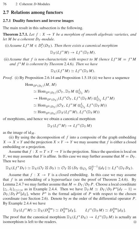
76 2 Coherent D-Modules
2.7 Relations among functors
2.7.1 Duality functors and inverse images
The main result in this subsection is the following.
Theorem 2.7.1. Let f : X → Y be a morphism of smooth algebraic varieties, andlet M be a coherent DY -module.
(i) Assume Lf ∗M ∈ Dbc (DX). Then there exists a canonical morphism
DX(Lf ∗M) → Lf ∗(DY M).
(ii) Assume that f is non-characteristic with respect to M (hence Lf ∗M = f ∗M
and f ∗M is coherent by Theorem 2.4.6). Then we have
DX(Lf ∗M) � Lf ∗(DY M).
Proof. (i) By Proposition 2.6.14 and Proposition 1.5.18 (ii) we have a sequence
HomDb(DY )(M, M)
� HomDb(DY )(OY , DY M ⊗LOY
M)
→ HomDb(DX)(Lf ∗OY , Lf ∗(DY M) ⊗LOX
Lf ∗M)
� HomDb(DX)(OX, Lf ∗M ⊗LOX
Lf ∗(DY M))
� HomDb(DX)(DX(Lf ∗M), Lf ∗(DY M))
of morphisms, and hence we obtain a canonical morphism
DX(Lf ∗M) → Lf ∗(DY M)
as the image of idM .(ii) By using the decomposition of f into a composite of the graph embedding
X → X × Y and the projection X × Y → Y we may assume that f is either a closedembedding or a projection.
Assume that f : X = T ×Y → Y is the projection. Since the question is local onY , we may assume that Y is affine. In this case we may further assume that M = DY .Then we have
DX(Lf ∗DY ) � DX(OT � DY ) � OT � (DY ⊗OY�⊗−1
Y )[dY ] � Lf ∗(DY DX).
Assume that f : X → Y is a closed embedding. In this case we may assumethat f is an embedding of a hypersurface (see the proof of Theorem 2.4.6). ByLemma 2.4.7 we may further assume that M = DY /DY P . Choose a local coordinate{zi, ∂i}1≤i≤n as in Example 2.4.4. Then we have DY M � DY /DY P ∗[dY − 1] =DY /DY P ∗[dX], where P ∗ is the formal adjoint of P with respect to the chosencoordinate (see Section 2.6). Denote by m the order of the differential operator P .By Example 2.4.4 we have
DX(Lf ∗M) � DX(D⊕mX ) � D⊕m
X [dX], Lf ∗(DY M) � D⊕mX [dX].
The proof that the canonical morphism DX(Lf ∗DX) → Lf ∗(DY M) is actually anisomorphism is left to the readers. ��
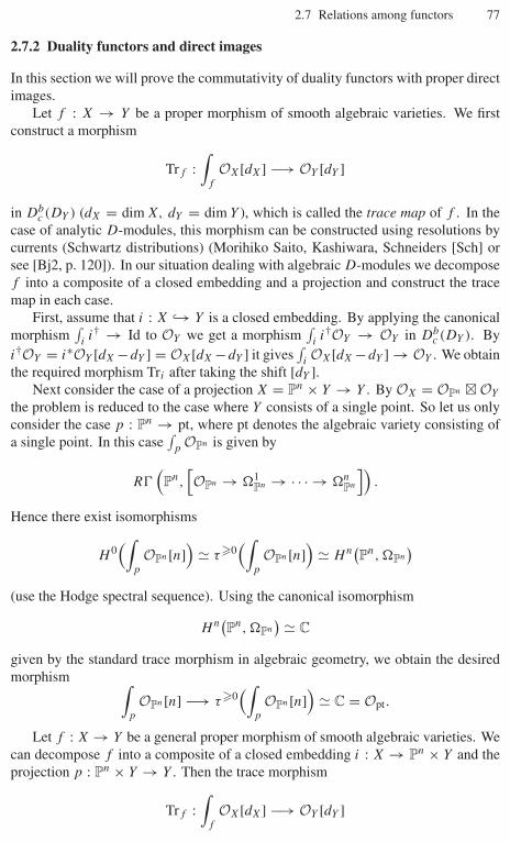
2.7 Relations among functors 77
2.7.2 Duality functors and direct images
In this section we will prove the commutativity of duality functors with proper directimages.
Let f : X → Y be a proper morphism of smooth algebraic varieties. We firstconstruct a morphism
Trf :∫
f
OX[dX] −→ OY [dY ]
in Dbc (DY ) (dX = dim X, dY = dim Y ), which is called the trace map of f . In the
case of analytic D-modules, this morphism can be constructed using resolutions bycurrents (Schwartz distributions) (Morihiko Saito, Kashiwara, Schneiders [Sch] orsee [Bj2, p. 120]). In our situation dealing with algebraic D-modules we decomposef into a composite of a closed embedding and a projection and construct the tracemap in each case.
First, assume that i : X ↪→ Y is a closed embedding. By applying the canonicalmorphism
∫ii† → Id to OY we get a morphism
∫ii†OY → OY in Db
c (DY ). Byi†OY = i∗OY [dX −dY ] = OX[dX −dY ] it gives
∫iOX[dX −dY ] → OY . We obtain
the required morphism Tri after taking the shift [dY ].Next consider the case of a projection X = Pn × Y → Y . By OX = OPn � OY
the problem is reduced to the case where Y consists of a single point. So let us onlyconsider the case p : Pn → pt, where pt denotes the algebraic variety consisting ofa single point. In this case
∫p
OPn is given by
R�(Pn,
[OPn → �1
Pn → · · · → �nPn
]).
Hence there exist isomorphisms
H 0(∫
p
OPn [n])
� τ�0(∫
p
OPn [n])
� Hn(Pn, �Pn
)(use the Hodge spectral sequence). Using the canonical isomorphism
Hn(Pn, �Pn
) � C
given by the standard trace morphism in algebraic geometry, we obtain the desiredmorphism ∫
p
OPn [n] −→ τ�0(∫
p
OPn [n])
� C = Opt.
Let f : X → Y be a general proper morphism of smooth algebraic varieties. Wecan decompose f into a composite of a closed embedding i : X → Pn × Y and theprojection p : Pn × Y → Y . Then the trace morphism
Trf :∫
f
OX[dX] −→ OY [dY ]

78 2 Coherent D-Modules
is defined as the composite of∫f
OX[dX] =∫
p
∫i
OX[dX] −→∫
p
OPn×Y [dY + n] −→ OY [dY ].
One can show that the trace morphism Trf does not depend on the choice of thedecomposition f = p ◦ i and that it is functorial in the sense that for two propermorphisms f : X → Y and g : Y → Z we have Trg◦f = Trg ◦ ∫
gTrf . We omit the
details.The main result in this section is the following.
Theorem 2.7.2. Let f : X → Y be a proper morphism. Then we have a canonicalisomorphism ∫
f
DX∼−→ DY
∫f
: Dbc (DX) −→ Db
c (DY )
of functors.
Proof. We first construct a canonical morphism∫
fDX → DY
∫f
of functors. Let
M · ∈ Dbc (DX). By∫
f
DXM = Rf∗(RHomDX(M ·, DX) ⊗L
DXDX→Y ) ⊗L
OY�⊗−1
Y [dX]
= Rf∗(RHomDX(M ·, DX→Y )) ⊗L
OY�⊗−1
Y [dX],DY
∫f
M = RHomDY
(∫f
M ·, DY
)⊗L
OY�⊗−1
Y [dY ],
it is sufficient to construct a canonical morphism
�(M ·) : Rf∗(RHomDX(M ·, DX→Y [dX])) → RHomDY
(∫f
M ·, DY [dY ])
in Dbc (D
opY ). By the projection formula (Corollary 1.7.5) we have∫
f
DX→Y [dX] =∫
f
Lf ∗DY [dX] �∫
f
OX[dX] ⊗LOY
DY
and hence the trace morphism Trf induces a canonical morphism∫f
DX→Y [dX] → DY [dY ].
Using this �(M ·) is defined as the composite of
Rf∗(RHomDX(M ·, DX→Y [dX]))
→ Rf∗RHomf −1DY(DY←X ⊗L
DXM ·, DY←X ⊗L
DXDX→Y [dX]))
→ RHomDY(Rf∗(DY←X ⊗L
DXM ·), Rf∗(DY←X ⊗L
DXDX→Y )[dX])
2.7 Relations among functors 79
= RHomDY
(∫f
M ·,∫
f
DX→Y [dX])
→ RHomDY
(∫f
M ·, DY [dY ]).
It remains to prove that �(M ·) is an isomorphism for any M ·. By decomposingf into a composite of a closed embedding and a projection we may assume fromthe beginning that f is either a closed embedding i : X ↪→ Y or a projectionp : X = Pn ×Y → Y . In each case there exists locally on Y a resolution F · � M · ofM · in Db
c (DX), where F · is a bounded complex of DX-modules such that each termF j of F · is a direct summand of a free DX-module of finite rank. This is obvious inthe case of a closed embedding. In the case of a projection this is a consequence ofTheorem 1.6.5 and Proposition 1.4.13. Therefore, we may assume from the beginningthat M · = DX (see the proof of Theorem 2.5.1).
Let i : X ↪→ Y be a closed embedding. In this case �(DX) is given by thecomposite of
i∗(RHomDX(DX, i∗DY )[dX]
� RHomDY
(∫i
DX,
∫i
i∗DY
)[dX]
= RHomDY
(∫i
DX,
∫i
i†DY
)[dY ]
→ RHomDY
(∫i
DX, DY
)[dY ],
where the first isomorphism is a consequence of Kashiwara’s equivalence. Henceit is sufficient to show that RHomDY
(∫
iDX,
∫ii†DY ) → RHomDY
(∫
iDX, DY ) is
an isomorphism. Set U = Y \ X and let j : U → X be the embedding. By thedistinguished triangle ∫
i
i†DY −→ DY −→∫
j
j†DY+1−→
we have only to show that RHomDY(∫
iDX,
∫j
j∗DY ) = 0. By Propositions 1.5.25and 1.7.1 (ii), we obtain
RHomDY
(∫i
DX,
∫j
j∗DY
)� i∗RHomDX
(DX, i!
∫j
j∗DY
)= i∗i!
∫j
j∗DY = 0.
Let p : X = Pn × Y → Y be the projection. By DX = DPn � DY the problem iseasily reduced to the case when Y consists of a single point and we can only considerthe case p : X = Pn → pt, where pt is the algebraic variety consisting of a singlepoint. In this case we have DPn→pt = OPn , Dpt←Pn = �Pn and hence

80 2 Coherent D-Modules
Rp∗(RHomDX(DX, DX→Y [dX]))
= R HomDPn (DPn , OPn)[n] = R�(Pn, OPn)[n] � C[n],RHomDY
(∫p
DX, DY [dY ])
= R HomC(R�(Pn, �nP), C) � HomC(C[−n], C) = C[n].
Therefore, it is sufficient to show that �(DPn) is non-trivial. Note that �(DPn)[−n]is given by the composite of
R HomDPn (DPn , OPn)
→ R HomC(�Pn , �Pn ⊗LDPn
OPn)
→ R HomC(R�(Pn, �Pn), R�(Pn, �Pn ⊗LDPn
OPn))
→ R HomC(R�(Pn, �Pn), τ�nR�(Pn, �Pn ⊗LDPn
OPn))
� R HomC(R�(Pn, �Pn), C[−n])� R HomC(R�(Pn, �Pn), R�(Pn, �Pn)).
We easily see that the morphism
R HomDPn (DPn , OPn) → R HomC(R�(Pn, �Pn), R�(Pn, �Pn))
is induced by the canonical morphism OPn → HomOPn (�Pn , �Pn) and it is non-trivial. ��Corollary 2.7.3 (Adjunction formula). Let f : X → Y be a proper morphism.Then we have an isomorphism
RHomDY
(∫f
M ·, N ·) � Rf∗RHomDX(M ·, f †N ·)
for M · ∈ Dbc (DX) and N · ∈ Db(DY ).
Proof. We have
Rf∗RHomDX(M ·, f †N ·)
� Rf∗((�X ⊗LOX
DXM ·) ⊗LDX
Lf ∗N ·)[−dY ]� Rf∗((�X ⊗L
OXDXM ·) ⊗L
DXDX→Y ⊗L
f −1DYf −1N ·)[−dY ]
� Rf∗((�X ⊗LOX
DXM ·) ⊗LDX
DX→Y ) ⊗LDY
N ·[−dY ]�∫
f
DXM · ⊗LDY
N ·[−dY ]
� DY
∫f
M · ⊗LDY
N ·[−dY ]
� RHomDY
(∫f
M ·, N ·)by Proposition 2.6.14 and Theorem 2.7.2. ��
3
Holonomic D-Modules
In this chapter we study functorial behaviors of holonomic systems and show thatany simple object in the abelian category of holonomic DX-modules is a minimalextension of an integrable connection on a locally closed smooth subvariety Y of X.
3.1 Basic results
Recall that the dimension of the characteristic variety Ch(M) of a coherent DX-module M (= 0) satisfies the inequality dim Ch(M) ≥ dim X and that a coherentDX-module M is called holonomic if dim Ch(M) = dim X or M = 0.
Notation 3.1.1. We denote by Modh(DX) the full subcategory of Modc(DX) con-sisting of holonomic DX-modules.
The next proposition implies that Modh(DX) is a thick abelian subcategory ofModc(DX).
Proposition 3.1.2.(i) For an exact sequence
0 → M → N → L → 0
in Modc(DX) we have
N ∈ Modh(DX) ⇐⇒ M, L ∈ Modh(DX).
(ii) Any holonomic DX-module has finite length. In other words, the categoryModh(DX) is artinian.
Proof. The statement (i) is a consequence of Ch(N) = Ch(M) ∪ Ch(L).The statement (ii) is proved using the characteristic cycle as follows. For a
holonomic DX-module M consider its characteristic cycle
CC(M) =∑
C∈I (Ch(M))
mC(M) C.
82 3 Holonomic D-Modules
Note that dim C = dX for any C ∈ I (Ch(M)). Define the total multiplicity of M by
m(M) :=∑
C∈I (Ch(M))
mC(M).
By Theorem 2.2.3 the total multiplicity is additive in the sense that we have m(M) =m(L) + m(N) for any short exact sequence
0 → L → M → N → 0
in Modh(DX). Moreover, we have m(M) = 0 ⇐⇒ Ch(M) = ∅ ⇐⇒ M = 0 bythe definition of characteristic varieties. Hence the assertion follows by inductionon m(M). ��Notation 3.1.3. We denote by Db
h(DX) the full subcategory of Dbc (DX) consisting of
objects M · ∈ Dbc (DX) whose cohomology groups are holonomic, that is, Hi(M ·) ∈
Modh(DX) for ∀i ∈ Z.
We easily see the following from Propositions 3.1.2 and B.4.7.
Corollary 3.1.4. Dbh(DX) is a full triangulated subcategory of Db
c (DX).
Remark 3.1.5. It is known that
Db(Modh(DX))∼→ Db
h(DX)
(see Beilinson [Bei]).
The following result is the first important step in the study of holonomic D-modules. Namely, we can say “A holonomic D-module is generically an integrableconnection.’’
Proposition 3.1.6. Let M be a holonomic DX-module. Then there exists an opendense subset U ⊂ X such that M|U is coherent over OU . In other words, M|U is anintegrable connection on U .
Proof. Let T ∗XX ⊂ T ∗X be the zero section of T ∗X and set S := Ch(M) \ T ∗
XX. IfS = ∅, then M itself is coherent over OX by Proposition 2.2.5. Assume that S = ∅.Since S is conic, the dimension of each fiber of π |S : S � π(S) (π : T ∗X → X) is≥ 1 and hence dim π(S) < dim S ≤ dim X. Therefore, there exists an open subsetU ⊂ X such that X \ π(S) ⊃ U = ∅. In this case we have Ch(M|U ) \ T ∗
U U = ∅and hence M|U is coherent over OU by Proposition 2.2.5. ��
The following result, which can be proved by duality, is also important.
Proposition 3.1.7. Let M ∈ Modqc(DX). For an open subset U ⊂ X suppose thatwe are given a holonomic submodule N of M|U . Then there exists a holonomicsubmodule N of M such that N |U = N .
3.2 Functors for holonomic D-modules 83
Proof. By Corollary 1.4.17 we may assume that M is coherent and M|U = N . SetL = H 0(DXM). By Corollary 2.6.8 (ii) we have codim Ch(L) ≥ dX and henceL is a holonomic DX-module. Moreover, its dual N = DXL is also holonomic byCorollary 2.6.8 (vi). By L = H 0(DXM) � τ�0(DXM) we have a distinguishedtriangle
K · −→ DXM −→ L+1−→,
where K · = τ�−1(DXM). By applying DX we obtain
N −→ M −→ DXK · +1−→ .
Since the duality functors commute with restrictions to open subsets, we have
N |U = DU (L|U ) = D2U (M|U ) = M|U = N.
It remains to show that the canonical morphism N → M is injective. For this wehave only to show H−1(DXK ·) = 0. In fact, we will show that
Hi(DX(τ�−kK ·)) = 0 (i < 0, k > 0) (3.1.1)
(note that τ�−kK · � K · for k � 0). Let us first show
Hi(DX(H−k(K ·)[k])) = 0 (i < 0, k > 0). (3.1.2)
For k > 0 we have H−k(K ·) � H−k(DXM) and hence codim Ch(H−k(K ·)) ≥ dX−k by Corollary 2.6.8 (ii). Hence the assertion is a consequence of Corollary 2.6.8 (i).Now we prove (3.1.1) by induction on k. If k = 1, then we have τ�−kK · =H−k(K ·)[k], and hence the assertion follows from (3.1.2). Assume k � 2. Byapplying DX to the distinguished triangle
H−k(K ·)[k] −→ τ�−kK · −→ τ�−(k−1)K · +1−→we obtain a distinguished triangle
DX(τ�−(k−1)K ·) −→ DX(τ�−kK ·) −→ DX(H−k(K ·)[k]) +1−→ .
Hence the assertion follows from (3.1.2) and the hypothesis of induction. ��
3.2 Functors for holonomic D-modules
3.2.1 Stability of holonomicity
We first note the following, which is an obvious consequence of Corollary 2.6.8.
Proposition 3.2.1. The duality functor DX induces isomorphisms
DX : Modh(DX) −→∼ Modh(DX)op,
DX : Dbh(DX) −→∼ Db
h(DX)op.
84 3 Holonomic D-Modules
The following is also obvious by Ch(M � N) = Ch(M) × Ch(N).
Proposition 3.2.2. The external tensor product � induces the functors
(•) � (•) : Modh(DX) × Modh(DY ) → Modh(DX×Y ),
(•) � (•) : Dbh(DX) × Db
h(DY ) → Dbh(DX×Y ).
Recall that for a morphism f : X → Y of smooth algebraic varieties we havefunctors ∫
f
: Dbqc(DX) −→ Db
qc(DY ),
f † : Dbqc(DY ) −→ Db
qc(DX).
Moreover, if f is proper (resp. smooth),∫
f(resp. f †) preserves the coherency and
we have the functors∫f
: Dbc (DX) → Db
c (DY ) (resp. f † : Dbc (DY ) → Db
c (DX)).
However, neither∫
fnor f † preserves the coherency for general morphisms f . A
surprising fact, which we will show in this section, is that the holonomicity is never-theless preserved by these functors for any morphism f : X → Y . Namely, we havethe following.
Theorem 3.2.3. Let f : X → Y be a morphism of smooth algebraic varieties.
(i)∫
fsends Db
h(DX) to Dbh(DY ).
(ii) f † sends Dbh(DY ) to Db
h(DX).
Corollary 3.2.4. The internal tensor product ⊗LOX
induces the functor
(•) ⊗LOX
(•) : Dbh(DX) × Db
h(DX) → Dbh(DX).
Proof. This follows from Proposition 3.2.2 and Theorem 3.2.3 (ii) noting that (•)⊗LOX
(•) = L�∗X ◦ ((•) � (•)), where �X : X → X × X is the diagonal embedding. ��
The proof of Theorem 3.2.3 will be completed in the next subsection. In the restof this subsection we reduce it to that of Theorem 3.2.3 (i) in the case when f is theprojection Cn → Cn−1.
Lemma 3.2.5. Let i : X → Y be a closed embedding. Then for M · ∈ Dbc (DX)
we have
M · ∈ Dbh(DX) ⇐⇒
∫i
M · ∈ Dbh(DY ).

3.2 Functors for holonomic D-modules 85
Proof. Since∫
iis exact, we may assume that M = M · ∈ Modc(DX). Let
T ∗Y�←↩ X ×Y T ∗Y
ρ� T ∗X
be the canonical morphisms. Then we have
Ch(∫
i
M)
= �ρ−1(Ch(M)),
by Lemma 2.3.5. Since � is a closed embedding and ρ is a smooth surjectivemorphism with one-dimensional fibers, we have
dim Ch(∫
i
M)
= dim Ch(M) + 1,
form which we obtain the desired result. ��Next we reduce the proof of Theorem 3.2.3 (i) to the case when f is the pro-
jection Cn → Cn−1. In order to prove Theorem 3.2.3 (i) it is sufficient to show∫f
M ∈ Dbh(DY ) for M ∈ Modh(DX). By considering the decomposition of f into
a composite of a closed embedding and a projection we may assume that f is either aclosed embedding or a projection. The case of a closed embedding has already beendealt with in Lemma 3.2.5, and hence we can only consider the case when f is theprojection X = Z × Y → Y . Since the problem is local on Y , we may assume thatY is affine. Take a finite affine open covering Z = ⋃r
i=0 Zi of Z such that Z \ Zi isa divisor on Z for each i, and set Xi = Zi × Y . Then X = ⋃r
i=0 Xi is an affine opencovering of X. For 0 ≤ i0 < · · · < ik ≤ r let ji0,...,ik : Xi0,...,ik = ⋂k
p=0 Xip → X
be the embedding (note that Xi0,...,ik is affine by the choice of Zi’s). Then M isquasi-isomorphic to the Cech complex
· · · −→ 0 −→ C0(M) −→ C1(M) −→ · · · −→ Cr(M) −→ 0 −→ · · ·with
Ck(M) =⊕
i0<···<ik
ji0,...,ik∗(M|Xi0,...,ik)
(note ji0,...,ik∗(M|Xi0,...,ik) � ∫
ji0,...,ikj∗i0,...,ik
M). Hence it is sufficient to show∫f ◦ji0,...,ik
j∗i0,...,ik
M(= ∫f
∫ji0,...,ik
j∗i0,...,ik
M) ∈ Dbh(DY ) for any (i0, . . . , ik). There-
fore, we may assume from the beginning that X and Y are affine. Fix closed embed-dings α : X ↪→ Cn, β : Y ↪→ Cm, and consider the commutative diagram
X Y
X × Y
Cn+m Cm,
�f
�g
�
β
�α×β
�p
86 3 Holonomic D-Modules
where g is the graph embedding associated to f and p is the projection. ByLemma 3.2.5
∫f
M ∈ Dbh(DY ) if and only if
∫β
∫f
M ∈ Dbh(DCm). Note that∫
β
∫f
M =∫
β◦f
M =∫
p
∫(α×β)◦g
M.
Since (α × β) ◦ g is a closed embedding, we have∫(α×β)◦g
M ∈ Modh(DCn+m)
by Lemma 3.2.5, and hence the problem is reduced to the case when f is the projectionCn+m → Cm. Since Cn+m → Cm is a composite of morphisms Ck → Ck−1, theproblem is finally reduced to the case when f is the projection Cn → Cn−1.
Let us show that Theorem 3.2.3 (i) implies Theorem 3.2.3 (ii). So we assumethat Theorem 3.2.3 (i) holds and show f †M ∈ Db
h(DX) for any M ∈ Modh(DY ).By decomposing f into a composite of a closed embedding and a projection we mayfurther assume that f is either a closed embedding or a projection. Consider first thecase where f is the projection X = Z ×Y → Y . Then f ∗ is an exact functor and thecomplex f †M = f ∗M[dim Z] is concentrated in the degree − dim Z. Moreover, wehave f ∗M � OZ � M and it is holonomic by
Ch(OZ � M) = Ch(OZ) × Ch(M) = T ∗ZZ × Ch(M),
and hence f †M ∈ Dbh(DX). Let us consider the case of a closed embedding i : X ↪→
Y . Let j : U := Y \ X ↪→ Y be the corresponding open embedding. Then by theresults in Section 1.7 there exists a distinguished triangle∫
i
i†M −→ M −→∫
j
j†M+1−→ .
We have j†M = M|U ∈ Modh(DU ), and hence (i) implies∫
jj†M · ∈ Db
h(DY ).
Therefore, we see by the above distinguished triangle that∫
ii†M · ∈ Db
h(DY ). Thisimplies i†M · ∈ Db
h(DX) by Lemma 3.2.5. Theorem 3.2.3 (ii) is verified assumingTheorem 3.2.3 (i).
3.2.2 Holonomicity of modules over Weyl algebras
In the last subsection the proof Theorem 3.2.3 (i), (ii) was reduced to that of (i) inthe case when f is the projection p : Cn = C × Cn−1 → Cn−1. The aim of thissubsection is to prove it using the theory of D-modules on Cn.
SetDn := �(Cn, DCn) =
⊕α,β
Cxα∂β,
where xα = xα11 x
α22 · · · xαn
n for α = (α1, . . . , αn) and ∂β = ∂β11 ∂
β22 · · · ∂βn
n for β =(β1, . . . , βn). The algebra Dn is called the Weyl algebra. Since Cn is affine, we haveequivalences of categories
3.2 Functors for holonomic D-modules 87
Modqc(DCn) −→∼ Mod(Dn),
Modc(DCn) −→∼ Modf (Dn)
given by M �→ �(Cn, M). For N ∈ Mod(Dn) we denote the corresponding DCn -module by N . A Dn-module N is called holonomic if N is a holonomic DCn -module.
Let N be a Dn-module. We define its Fourier transform N as follows. As anadditive group N is the same as N , and the action of the generators xi, ∂i of Dn onN is given by
xi ◦ s := − ∂is, ∂i ◦ s := xis.
It is easily checked that N is a left Dn-module with respect to this action ◦. Thisdefinition of the Fourier transform N is motivated by the classical Fourier transform.The Fourier transform induces equivalences of categories
(•) : Mod(Dn) −→∼ Mod(Dn),
(•) : Modf (Dn) −→∼ Modf (Dn).
The corresponding equivalences for the categories of DCn -modules are also de-noted by
(•) : Modqc(DCn) −→∼ Modqc(DCn),
(•) : Modc(DCn) −→∼ Modc(DCn).
Proposition 3.2.6. Let p : Cn(= C × Cn−1) → Cn−1 be the projection and let i :Cn−1(= {0}×Cn−1) ↪→ Cn(= C×Cn−1) be the embedding. For M ∈ Modqc(DCn)
we have
Hk(∫
p
M)
� Hk(Li∗M)
for any k.
Proof. Set N = �(Cn, M). Since p is an affine morphism, we have∫p
M � Rp∗(DRCn/Cn−1(M)) � [p∗M
∂1−→ p∗M],
and hence
�
(Cn−1, Hk
(∫p
M))
�
⎧⎪⎪⎨⎪⎪⎩Ker
[N
∂1−→ N]
(k = −1),
Coker[N
∂1−→ N]
(k = 0),
0 (k = 0, −1).
Therefore, we have
88 3 Holonomic D-Modules
�
(Cn−1,
Hk(∫
p
M))
�
⎧⎪⎨⎪⎩Ker
[N
x1−→ N]
(k = −1),
Coker[N
x1−→ N]
(k = 0),
0 (k = 0, −1),
� �(Cn−1, Hk(Li∗M))
from which we obtain the desired result. ��In proving Theorem 3.2.3 we also need the following results.
Proposition 3.2.7. A coherent DCn -module M is holonomic if and only if M is as well.
Proposition 3.2.8. Let j : (C \ {0}) × Cn−1 → Cn be the embedding. If M is aholonomic DCn -module, then so is H 0(
∫j
j†M) (since (C \ {0}) × Cn−1 is an affine
open subset of Cn we have Hk(∫
jj†M) = 0 for k = 0).
Let us complete the proof of Theorem 3.2.3 assuming Propositions 3.2.7 and 3.2.8.By Propositions 3.2.6 and 3.2.7 and the arguments in the last subsection it is sufficientto show i†M ∈ Db
h(DCn−1) for M ∈ Modh(DCn), where i : Cn−1 ↪→ Cn is as inProposition 3.2.6. Let j : (C \ {0}) × Cn−1 ↪→ Cn be as in Proposition 3.2.8. By thedistinguished triangle ∫
i
i†M −→ M −→∫
j
j†M+1−→
we obtain an exact sequence
0 −→ H 0(∫
i
i†M)
−→ M −→ H 0(∫
j
j†M)
−→ H 1(∫
i
i†M)
−→ 0.
Since H 0(∫
jj†M) is holonomic by Proposition 3.2.8, we obtain
∫ii†M ∈ Db
h(DCn)
(note Hk(∫
ii†M) = 0 for k = 0, 1). Hence we have i†M ∈ Db
h(DCn−1) byLemma 3.2.5.
The rest of this subsection is devoted to proving Proposition 3.2.7 and Proposi-tion 3.2.8.
In addition to the usual order filtration F , the Weyl algebra Dn has another filtrationB defined by
BiDn :=∑
|α|+|β|≤i
Cxα∂β ⊂ Dn.
We call it the Bernstein filtration of the Weyl algebra Dn. The graded algebra grB Dn
associated to the Bernstein filtration B is commutative and isomorphic to the poly-nomial ring C[x, ξ ] (x = (x1, x2, . . . , xn), ξ = (ξ1, ξ2, . . . , ξn)), as in the case ofthe usual order filtration. For a Dn-module M we can also define good filtrations F
on it with respect to the Bernstein filtration B. Any finitely generated Dn-modulehas a good filtration. The Bernstein filtration has the advantage that for any goodfiltration F of a finitely generated Dn-module M each FiM is finite dimensional overC. Therefore, we can apply results on Hilbert polynomials to the associated gradedgrB Dn-module.
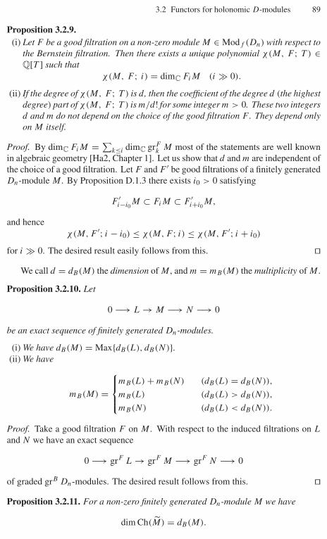
3.2 Functors for holonomic D-modules 89
Proposition 3.2.9.(i) Let F be a good filtration on a non-zero module M ∈ Modf (Dn) with respect to
the Bernstein filtration. Then there exists a unique polynomial χ(M, F ; T ) ∈Q[T ] such that
χ(M, F ; i) = dimC FiM (i � 0).
(ii) If the degree of χ(M, F ; T ) is d , then the coefficient of the degree d (the highestdegree) part of χ(M, F ; T ) is m/d! for some integer m > 0. These two integersd and m do not depend on the choice of the good filtration F . They depend onlyon M itself.
Proof. By dimC FiM = ∑k≤i dimC grF
k M most of the statements are well knownin algebraic geometry [Ha2, Chapter 1]. Let us show that d and m are independent ofthe choice of a good filtration. Let F and F ′ be good filtrations of a finitely generatedDn-module M . By Proposition D.1.3 there exists i0 > 0 satisfying
F ′i−i0
M ⊂ FiM ⊂ F ′i+i0
M,
and henceχ(M, F ′; i − i0) ≤ χ(M, F ; i) ≤ χ(M, F ′; i + i0)
for i � 0. The desired result easily follows from this. ��We call d = dB(M) the dimension of M , and m = mB(M) the multiplicity of M .
Proposition 3.2.10. Let
0 −→ L → M −→ N −→ 0
be an exact sequence of finitely generated Dn-modules.
(i) We have dB(M) = Max{dB(L), dB(N)}.(ii) We have
mB(M) =
⎧⎪⎨⎪⎩mB(L) + mB(N) (dB(L) = dB(N)),
mB(L) (dB(L) > dB(N)),
mB(N) (dB(L) < dB(N)).
Proof. Take a good filtration F on M . With respect to the induced filtrations on L
and N we have an exact sequence
0 −→ grF L → grF M −→ grF N −→ 0
of graded grB Dn-modules. The desired result follows from this. ��Proposition 3.2.11. For a non-zero finitely generated Dn-module M we have
dim Ch(M) = dB(M).
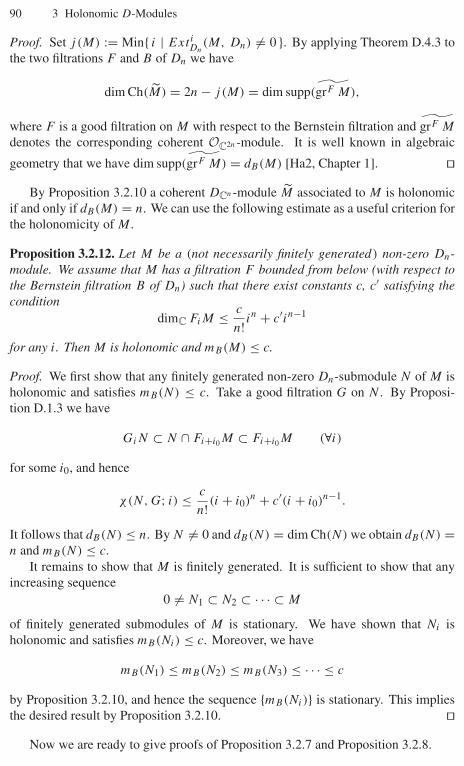
90 3 Holonomic D-Modules
Proof. Set j (M) := Min{ i | ExtiDn
(M, Dn) = 0 }. By applying Theorem D.4.3 tothe two filtrations F and B of Dn we have
dim Ch(M) = 2n − j (M) = dim supp(grF M),
where F is a good filtration on M with respect to the Bernstein filtration and grF M
denotes the corresponding coherent OC2n -module. It is well known in algebraic
geometry that we have dim supp(grF M) = dB(M) [Ha2, Chapter 1]. ��By Proposition 3.2.10 a coherent DCn -module M associated to M is holonomic
if and only if dB(M) = n. We can use the following estimate as a useful criterion forthe holonomicity of M .
Proposition 3.2.12. Let M be a (not necessarily finitely generated) non-zero Dn-module. We assume that M has a filtration F bounded from below (with respect tothe Bernstein filtration B of Dn) such that there exist constants c, c′ satisfying thecondition
dimC FiM ≤ c
n! in + c′in−1
for any i. Then M is holonomic and mB(M) ≤ c.
Proof. We first show that any finitely generated non-zero Dn-submodule N of M isholonomic and satisfies mB(N) ≤ c. Take a good filtration G on N . By Proposi-tion D.1.3 we have
GiN ⊂ N ∩ Fi+i0M ⊂ Fi+i0M (∀i)
for some i0, and hence
χ(N, G; i) ≤ c
n! (i + i0)n + c′(i + i0)n−1.
It follows that dB(N) ≤ n. By N = 0 and dB(N) = dim Ch(N) we obtain dB(N) =n and mB(N) ≤ c.
It remains to show that M is finitely generated. It is sufficient to show that anyincreasing sequence
0 = N1 ⊂ N2 ⊂ · · · ⊂ M
of finitely generated submodules of M is stationary. We have shown that Ni isholonomic and satisfies mB(Ni) ≤ c. Moreover, we have
mB(N1) ≤ mB(N2) ≤ mB(N3) ≤ · · · ≤ c
by Proposition 3.2.10, and hence the sequence {mB(Ni)} is stationary. This impliesthe desired result by Proposition 3.2.10. ��
Now we are ready to give proofs of Proposition 3.2.7 and Proposition 3.2.8.
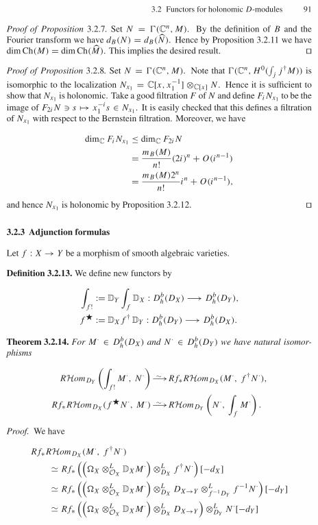
3.2 Functors for holonomic D-modules 91
Proof of Proposition 3.2.7. Set N = �(Cn, M). By the definition of B and theFourier transform we have dB(N) = dB(N). Hence by Proposition 3.2.11 we havedim Ch(M) = dim Ch(M). This implies the desired result. ��Proof of Proposition 3.2.8. Set N = �(Cn, M). Note that �(Cn, H 0(
∫j
j†M)) is
isomorphic to the localization Nx1 = C[x, x−11 ] ⊗C[x] N . Hence it is sufficient to
show that Nx1 is holonomic. Take a good filtration F of N and define FiNx1 to be theimage of F2iN s �→ x−i
1 s ∈ Nx1 . It is easily checked that this defines a filtrationof Nx1 with respect to the Bernstein filtration. Moreover, we have
dimC FiNx1 ≤ dimC F2iN
= mB(M)
n! (2i)n + O(in−1)
= mB(M)2n
n! in + O(in−1),
and hence Nx1 is holonomic by Proposition 3.2.12. ��
3.2.3 Adjunction formulas
Let f : X → Y be a morphism of smooth algebraic varieties.
Definition 3.2.13. We define new functors by∫f !
:= DY
∫f
DX : Dbh(DX) −→ Db
h(DY ),
f � := DXf † DY : Dbh(DY ) −→ Db
h(DX).
Theorem 3.2.14. For M · ∈ Dbh(DX) and N · ∈ Db
h(DY ) we have natural isomor-phisms
RHomDY
(∫f !
M ·, N ·)
−→∼ Rf∗RHomDX(M ·, f †N ·),
Rf∗RHomDX(f �N ·, M ·) −→∼ RHomDY
(N ·,
∫f
M ·)
.
Proof. We have
Rf∗RHomDX(M ·, f †N ·)
� Rf∗((
�X ⊗LOX
DXM ·)⊗LDX
f †N ·) [−dX]� Rf∗
((�X ⊗L
OXDXM ·)⊗L
DXDX→Y ⊗L
f −1DYf −1N ·) [−dY ]
� Rf∗((
�X ⊗LOX
DXM ·)⊗LDX
DX→Y
)⊗L
DYN ·[−dY ]
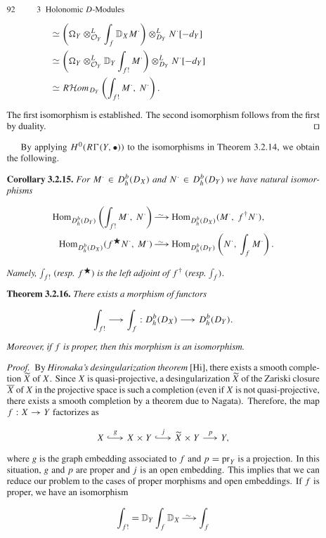
92 3 Holonomic D-Modules
�(
�Y ⊗LOY
∫f
DXM ·)
⊗LDY
N ·[−dY ]
�(
�Y ⊗LOY
DY
∫f !
M ·)
⊗LDY
N ·[−dY ]
� RHomDY
(∫f !
M ·, N ·)
.
The first isomorphism is established. The second isomorphism follows from the firstby duality. ��
By applying H 0(R�(Y, •)) to the isomorphisms in Theorem 3.2.14, we obtainthe following.
Corollary 3.2.15. For M · ∈ Dbh(DX) and N · ∈ Db
h(DY ) we have natural isomor-phisms
HomDbh(DY )
(∫f !
M ·, N ·)
−→∼ HomDbh(DX)(M
·, f †N ·),
HomDbh(DX)(f
�N ·, M ·) −→∼ HomDbh(DY )
(N ·,
∫f
M ·)
.
Namely,∫
f ! (resp. f �) is the left adjoint of f † (resp.∫
f).
Theorem 3.2.16. There exists a morphism of functors∫f !
−→∫
f
: Dbh(DX) −→ Db
h(DY ).
Moreover, if f is proper, then this morphism is an isomorphism.
Proof. By Hironaka’s desingularization theorem [Hi], there exists a smooth comple-tion X of X. Since X is quasi-projective, a desingularization X of the Zariski closureX of X in the projective space is such a completion (even if X is not quasi-projective,there exists a smooth completion by a theorem due to Nagata). Therefore, the mapf : X → Y factorizes as
Xg
↪−→ X × Yj
↪−→ X × Yp−→ Y,
where g is the graph embedding associated to f and p = prY is a projection. In thissituation, g and p are proper and j is an open embedding. This implies that we canreduce our problem to the cases of proper morphisms and open embeddings. If f isproper, we have an isomorphism∫
f != DY
∫f
DX −→∼∫
f
3.3 Finiteness property 93
by Theorem 2.7.2. So let us consider the case when f = j : X ↪→ Y is an openembedding. Let M · ∈ Db
h(DX). By Corollary 3.2.15 we have
HomDbh(DY )
(∫j !
M ·,∫
j
M ·)
� HomDbh(DX)
(M ·, j†
∫j
M ·)� HomDb
h(DX)(M·, M ·),
and hence we obtain the desired morphism∫j !
M · −→∫
j
M ·
as the image of id ∈ HomDbh(DX)(M
·, M ·). ��
3.3 Finiteness property
The aim of this section is to show the following.
Theorem 3.3.1. The following conditions on M · ∈ Dbc (DX) are equivalent:
(i) M · ∈ Dbh(DX).
(ii) There exists a decreasing sequence
X = X0 ⊃ X1 ⊃ · · · ⊃ Xm ⊃ Xm+1 = ∅of closed subsets of X such that Xr \ Xr+1 is smooth and all of the cohomologysheaves Hk(i
†r M ·) are integrable connections, where ir : Xr \ Xr+1 ↪→ X
denotes the embedding.(iii) For any x ∈ X all of the cohomology groups Hk(i
†xM ·) are finite dimensional
over C, where ix : {x} ↪→ X denotes the inclusion.
For the proof we need the following.
Lemma 3.3.2. Let M be a coherent (but not necessarily holonomic) DX-module.Then there exists an open dense subset U ⊂ X such that M|U is projective over OU .
Proof. Take a good filtration F of M . Then grF M is coherent over π∗OT ∗X. Itfollows from a well-known fact on coherent sheaves that there exists an open densesubset U ⊂ X such that (grF M)|U is free over π∗OT ∗U . By shrinking U if nec-essary we may assume that (grF M)|U is free over OU . This implies that each(FiM/Fi−1M)|U (and hence each FiM|U ) is projective over OU . ConsequentlyM|U is projective over OU . ��Proof of Theorem 3.3.1. (ii) ⇒ (i). Set Ur = X\Xr . We will show M ·|Ur ∈ Db
h(DUr )
by induction on r . Assume M ·|Ur ∈ Dbh(DUr ). Let j : Ur → Ur+1, i : Xr \ Xr+1
(= Ur+1 \ Ur) → Ur+1 be embeddings. Then we have a distinguished triangle

94 3 Holonomic D-Modules∫i
i†(M ·|Ur+1) −→ M ·|Ur+1 −→∫
j
j†(M ·|Ur+1)+1−→ .
By i†(M ·|Ur+1) = i†r M · ∈ Db
h(DXr\Xr+1) we have∫
ii†(M ·|Ur+1) ∈ Db
h(DUr+1).On the other hand by j†(M ·|Ur+1) = M ·|Ur ∈ Db
h(DUr ) we have∫
jj†(M ·|Ur+1) ∈
Dbh(DUr+1). Hence the above distinguished triangle implies M ·|Ur+1 ∈ Db
h(DUr+1).
(i) ⇒ (iii). By Theorem 3.2.3 we have i†xM · ∈ Db
h(D{x}). Note that D{x} � C.Hence the desired result follows from the fact that objects of Db
h(D{x}) = Dbc (D{x}) =
Dbc (Mod(C)) are just complexes of vector spaces whose cohomology groups are finite
dimensional.(iii) ⇒ (ii). It is sufficient to show that for any closed subset Y of X satisfying
Y ⊃ supp(M ·) := ⋃k supp(Hk(M ·)) there exists a decreasing sequence
Y = Y0 ⊃ Y1 ⊃ · · · ⊃ Ym ⊃ Ym+1 = ∅of closed subsets of Y such that Yr \ Yr+1 is smooth and all of the cohomologysheaves Hk(j
†r M ·) are integrable connections, where jr : Yr \Yr+1 ↪→ X denotes the
embedding. We will prove this statement by induction on dim Y . Take an open densesmooth subset V of Y , and let i : V → X denote the embedding. By Kashiwara’sequivalence we have i†M · ∈ Db
c (DV ). Hence by Lemma 3.3.2 there exists an opendense subset V ′ of V such that each cohomology sheaf Hk(i†M ·)|V ′ is projectiveover OV ′ . Therefore, by shrinking V if necessary we may assume from the beginningthat each cohomology sheaf Hk(i†M ·) is coherent over DV and projective over OV .We first show that Hk(i†M ·) is an integrable connection. Take x ∈ V and denote byjx : {x} ↪→ V the embedding. Then we have
C ⊗OV,xHk(i†M ·)x � Hk+dV (j
†x i†M ·) � Hk+dV (i
†xM ·),
where the first isomorphism follows from the fact that Hk(i†M ·)x is projective overOV,x . Hence the finite-dimensionality of Hk+dV (i
†xM ·) implies that the rank of the
projective OV,x-module Hk(i†M ·)x is finite. It follows that Hk(i†M ·) is coherentover OV , hence an integrable connection. Now take an open subset U of X such thatV = Y ∩ U , and let j : U → X be the embedding. Define N · by the distinguishedtriangle
N · −→ M · −→∫
j
j†M · +1−→ .
We easily see that∫
jj†M · � ∫
ii†M · ∈ Db
h(DX), and hence the above distinguished
triangle implies N · ∈ Dbc (DX). We also easily see that supp(N ·) ⊂ Y \V . Moreover,
for any locally closed smooth subset Z of Y \ V we have i†ZM · � i
†ZN ·, where iZ :
Z → X denotes the embedding. Indeed, we have i†Z
∫j
= 0 by Proposition 1.7.1 (ii).
In particular, for any x ∈ Y \V we have H ∗(i†xM ·) � H ∗(i
†xN ·). Hence by applying
the hypothesis of induction to N · there exists a decreasing sequence
Y \ V = Y1 ⊃ · · · ⊃ Ym ⊃ Ym+1 = ∅
3.4 Minimal extensions 95
of closed subsets of Y \ V such that Yr \ Yr+1 is smooth and all of the cohomologysheaves Hk(j
†r M ·) are integrable connections, where jr : Yr \ Yr+1 ↪→ X denotes
the embedding. Then the decreasing sequence
Y = Y0 ⊃ Y1 ⊃ · · · ⊃ Ym ⊃ Ym+1 = ∅satisfies the desired property. ��
3.4 Minimal extensions
A non-zero coherent D-module M is called simple if it contains no coherent D-submodules other than M or 0. Proposition 3.1.2 implies that for any holonomicD-module M there exists a finite sequence
M = M0 ⊃ M1 ⊃ · · · ⊃ Mr ⊃ Mr+1 = 0
of holonomic D-submodules such that Mi/Mi+1 is simple for each i (Jordan–Hölderseries of M). In this section we will give a classification of simple holonomic D-modules. More precisely, we will construct simple holonomic D-modules from inte-grable connections on locally closed smooth subvarieties using functors introducedin earlier sections, and show that any simple holonomic D-module is of this type.This construction corresponds via the Riemann–Hilbert correspondence to the mini-mal extension (Deligne–Goresky–MacPherson extension) in the category of perversesheaves.
Let Y be a (locally closed) smooth subvariety of a smooth algebraic variety X.Assume that the inclusion map i : Y ↪→ X is affine. Then DX←Y is locally freeover DY and Ri∗ = i∗ (higher cohomology groups vanish). Therefore, for a holo-nomic DY -module M we have Hj
∫iM = Hj
∫i! M = 0 for ∀j = 0. Namely, we
may regard∫
iM and
∫i! M as DX-modules. These DX-modules are holonomic by
Theorem 3.2.3. By Theorem 3.2.16 we have a morphism∫i!
M −→∫
i
M
in Modh(DX).
Definition 3.4.1. We call the image L(Y, M) of the canonical morphism∫
i! M −→∫iM the minimal extension of M .
By Proposition 3.1.2 the minimal extension L(Y, M) is a holonomic DX-module.
Theorem 3.4.2.(i) Let Y be a locally closed smooth connected subvariety of X such that i : Y → X is
affine, and let M be a simple holonomic DY -module. Then the minimal extensionL(Y, M) is also simple, and it is characterized as the unique simple submodule(resp. unique simple quotient module) of
∫iM (resp. of
∫i! M).
96 3 Holonomic D-Modules
(ii) Any simple holonomic DX-module is isomorphic to the minimal extensionL(Y, M) for some pair (Y, M), where Y is as in (i) and M is a simple inte-grable connection on Y .
(iii) Let (Y, M) be as in (ii), and let (Y ′, M ′) be another such pair. Then we haveL(Y, M) � L(Y ′, M ′) if and only if Y = Y ′ and M|U � M ′|U for an opendense subset U of Y ∩ Y ′.
Proof. (i) We choose an open subset U ⊂ X containing Y such that k : Y ↪→U is a
closed embedding. Let j : U ↪→ X be the embedding, and let ModYqc DX denote the
category of OX-quasi-coherent DX-modules whose support is contained in Y . Wefirst show the following four results:
(a) For any E ∈ ModYqc(DX) we have Hli†E = 0 (l = 0). Hence H 0i† = i� :
ModYqc(DX) → Modqc(DY ) is an exact functor.
(b) For any non-zero holonomic submodule N of∫
iM , we have i†N � M .
(c)∫
iM (resp.
∫i! M) has a unique simple holonomic submodule (resp. simple holo-
nomic quotient module).(d) For a sequence 0 = N1 ⊂ N2 ⊂ ∫
iM of holonomic submodules of
∫iM , we
have i†(N2/N1) = 0.
For E ∈ ModYqc(DX) we have i†E = k†j†E = k†j−1E and supp j−1E ⊂ Y .
Hence (a) is a consequence of Kashiwara’s equivalence.Let N be as in (b). By Corollary 3.2.15 we have
HomDX
(N,
∫i
M)
= HomDX
(N,
∫j
∫k
M)
� HomDU
(j�N,
∫k
M).
Since j is an open embedding, we have j� = j† = j−1. Therefore, the inclusionN ↪→ ∫
iM induces a non-zero morphism ϕ : j†N → ∫
kM . Since
∫kM is a simple
holonomic DU -module by Kashiwara’s equivalence, ϕ is surjective. Applying k† toit, we obtain a surjective morphism i†N � k†
∫kM � M . On the other hand, we
have an injective morphism i†N → i†∫
iM = M because i† is exact by (a). Hence
we must have i†N � M , and (b) is proved.Suppose there exist two simple holonomic submodules L = L′ of
∫iM . Set
N = L + L′ = L ⊕ L′. Then by (b) we have
M � i†N = i†L ⊕ i†L′ = M ⊕ M,
which is a contradiction. The assertion (c) for∫
iM is proved. Another assertion for∫
i! M is easily proved using the duality functor.By (a) we have
i†N1 ⊂ i†N2 ⊂ i†∫
i
M = M, i†N2/i†N1 � i†(N2/N1).
3.4 Minimal extensions 97
Hence (b) implies i†(N2/N1) = 0, and (d) is proved.Now let us finish the proof of (i). By (c) there exists a unique simple holonomic
submodule L of∫
iM . By Corollary 3.2.15 there exist two isomorphisms
HomDX
(∫i!
M, L)
� HomDY(M, i†L)
(b)� HomDY(M, M),
HomDX
(∫i!
M,
∫i
M)
� HomDY
(M, i†
∫i
M)
� HomDY(M, M),
from which we see that the canonical morphism∫
i! M → ∫iM is non-zero and
factorizes as∫
i! M → L ↪→ ∫iM . Since L is a simple module, the image of this
morphism should be L. This completes the proof of (i).(ii) Assume that L is a simple holonomic DX-module. We take an affine open
dense subset Y (i : Y ↪→ X) of an irreducible component of supp L so that i†L is anintegrable connection on Y (this is possible by Proposition 3.1.6). Set M = i†L. Weeasily see by Proposition 3.1.7 that M is simple. Moreover, by Corollary 3.2.15 weget an isomorphism
HomDX
(∫i!
M, L)
� HomDY(M, i†L) � HomDY
(M, M) = 0,
from which we see that there exists a non-zero surjective morphism∫
i! M → L.Namely, L is a simple holonomic quotient module of
∫i! M . Hence we obtain L =
L(Y, M) by (i). The assertion (ii) is proved.The proof for the last part (iii) is easy and left to the readers. ��
Proposition 3.4.3. Let Y be a locally closed smooth subvariety of X such that i :Y → X is affine, and let M be an integrable connection on Y . Then we have
DXL(Y, M) � L(Y, DY M).
Proof. By the exactness of the duality functor we obtain
DXL(Y, M) � Im(DX
∫i
M → DX
∫i!
M) � Im(
∫i!
DY M →∫
i
DY M)
= L(Y, DY M).
The proof is complete. ��
4
Analytic D-Modules and the de Rham Functor
Although our objectives in this book are algebraic D-modules (D-modules on smoothalgebraic varieties), we have to consider the corresponding analytic D-modules (D-modules on the underlying complex manifolds with classical topology) in definingtheir solution (and de Rham) complexes. In this chapter after giving a brief surveyof the general theory of analytic D-modules which are partially parallel to the theoryof algebraic D-modules given in earlier chapters we present fundamental proper-ties on the solution and the de Rham complexes. In particular, we give a proof ofKashiwara’s constructibility theorem for analytic holonomic D-modules. We notethat we also include another shorter proof of this important result in the special case ofalgebraic holonomic D-modules due to Beilinson–Bernstein. Therefore, readers whoare interested only in the theory of algebraic D-modules can skip reading Sections 4.4and 4.6 of this chapter.
4.1 Analytic D-modules
The aim of this section is to give a brief account of the theory of D-modules oncomplex manifolds. The proofs are occasionally similar to the algebraic cases andare omitted. Readers can refer to the standard textbooks such as Björk [Bj2] andKashiwara [Kas18] for details.
Let X be a complex manifold. It is regarded as a topological space via the clas-sical topology, and its dimension is denoted by dX. We denote by OX the sheaf ofholomorphic functions on X, and by �X, �
pX the sheaves of OX-modules consist-
ing of holomorphic vector fields and holomorphic differential forms of degree p,respectively (0 ≤ p ≤ dX). We also set �X = �
dX
X . The sheaf DX of holomorphicdifferential operators on X is defined as the subring of EndC(OX) generated by OX
and �X. In terms of a local coordinate {xi}1≤i≤n on a open subset U of X we have
DX|U =⊕α∈Nn
OU ∂α,
where
100 4 Analytic D-Modules and the de Rham Functor
∂i = ∂
∂xi
(1 ≤ i ≤ n), ∂α = ∂α11 · · · ∂αn
n (α = (α1, . . . , αn)).
We have the order filtration F = {FlDX}l≥0 of DX given by
FlDX|U =∑|α|≤l
OU ∂αx
(|α| =∑
i
αi
),
where U and {xi} are as above. It satisfies properties parallel to those in Proposi-tion 1.1.3, and DX turns out to be a filtered ring. The associated graded ring gr DX
is a sheaf of commutative algebras over OX, which is canonically regarded as asubalgebra of π∗OT ∗X, where π : T ∗X → X denotes the cotangent bundle of X.
Note that we have obvious analogies of the contents of Section 1.2, 1.3. Inparticular, we have an equivalence
�X ⊗OX(•) : Mod(DX) −→ Mod(D
opX )
between the categories Mod(DX), Mod(DopX ) of left and right DX-modules, respec-
tively. Moreover, for a morphism f : X → Y of complex manifolds we havea (DX, f −1DY )-bimodule DX→Y = OX ⊗f −1OY
f −1DY and an (f −1DY , DX)-
bimodule DY←X = �X ⊗OXDX→Y ⊗f −1OY
f −1�⊗−1Y . We say that a DX-module
is an integrable connection on X if it is locally free over OX of finite rank.
Notation 4.1.1. We denote by Conn(X) the category of integrable connections on thecomplex manifold X.
We have an analogy of Theorem 1.4.10. In particular, Conn(X) is an abeliancategory.
The following result is fundamental in the theory of analytic D-modules.
Theorem 4.1.2.(i) DX is a coherent sheaf of rings.
(ii) For any x ∈ X the stalk DX,x is a noetherian ring with left and right globaldimensions dim X.
The statement (i) follows from the corresponding fact for OX due to Oka, and (ii)is proved similarly to the algebraic case.
We can define the notion of a good filtration on a coherent DX-module as inSection 2.1. We remark that in our analytic situation a good filtration on a coherentDX-module exists only locally. In fact, there is an example of a coherent DX-modulewhich does not admit a global good filtration. Nevertheless, this local existence ofa good filtration is sufficient for many purposes. For example, we can define thecharacteristic variety Ch(M) of a coherent DX-module M as follows. For an opensubset U of X such that M|U admits a good filtration F we have a coherent OT ∗U -
module ˜grF (M|U ) := OT ∗U ⊗π−1
U gr DUπ−1
U grF M|U , where πU : T ∗U → U
denotes the projection. Then the characteristic variety Ch(M) is defined to be the
closed subvariety of T ∗X such that Ch(M) ∩ T ∗U = supp( ˜grF (M|U )) for any U
and F as above. It is shown to be well defined by Proposition D.1.3.As in the algebraic case we have the following.
4.1 Analytic D-modules 101
Theorem 4.1.3. For any coherent DX-module M its characteristic variety Ch(M) isinvolutive with respect to the canonical symplectic structure of the cotangent bun-dle T ∗X. In particular, for any irreducible component � of Ch(M), we have thatdim � ≥ dim X.
We say that a coherent DX-module M is holonomic if it satisfies
dim Ch(M) ≤ dim X.
Notation 4.1.4.(i) We denote by Modc(DX) (resp. Modh(DX)) the category of coherent (resp.
holonomic) DX-modules.(ii) We denote by Db
c (DX) (resp. Dbh(DX)) the subcategory of Db(DX) consisting
of M · ∈ Db(DX) satisfying Hi(M ·) ∈ Modc(DX) (resp. Modh(DX)) for any i.
As in Section 2.6 we can define the duality functor DX : Dbc (DX) → Db
c (DX)op
satisfying D2X � Id by
DXM · = RHomDX(M ·, DX ⊗OX
�⊗−1X [dX]).
All of the arguments in Section 2.6 are also valid for analytic D-modules. In particular,DX induces DX : Modh(DX) → Modh(DX)op.
Let f : X → Y be a morphism of complex manifolds. The functors
Lf ∗ : Db(DY ) → Db(DX) (M · �→ DX→Y ⊗Lf −1DY
f −1M ·),
f † : Db(DY ) → Db(DX) (M · �→ Lf ∗M ·[dX − dY ])are called the inverse image functors. Note that the boundedness of Lf ∗M · followsfrom Theorem 4.1.2 (ii). The notion that f : X → Y is non-characteristic withrespect to a coherent DY -module M is defined similarly to the algebraic case, and wehave the following analogy of Theorems 2.4.6 and 2.7.1.
Theorem 4.1.5. Let f : X → Y be a morphism of complex manifolds and let M bea coherent DY -module. Assume that f is non-characteristic with respect to M .
(i) Hj (Lf ∗M) = 0 for ∀j = 0.(ii) H 0(Lf ∗M) is a coherent DY -module.
(iii) Ch(H 0(Lf ∗M)) ⊂ ρf �−1f (Ch(M)).
(iv) DX(Lf ∗M) � Lf ∗(DY M).
Here, ρf : X ×Y T ∗Y → T ∗X and �f : X ×Y T ∗Y → T ∗Y are the canonicalmorphisms.
The proof is more or less the same as that for Theorem 2.4.6, 2.7.1.For a morphism f : X → Y of complex manifolds we can also define the direct
image functor∫f
: Db(DX) → Db(DY ) (M · �→ Rf∗(DY←X ⊗LDX
M ·)).

102 4 Analytic D-Modules and the de Rham Functor
The fact that∫
fpreserves the boundedness can be proved as follows. By decomposing
f into a composite of a closed embedding and a projection we may assume that f
is either a closed embedding or a projection. The case of a closed embedding iseasy. Assume that f : X = Y × Z → Y is a projection. We may assume thatM · = M ∈ Mod(DX). As in the algebraic case we have
∫f
M = Rf∗(DRX/Y M),where DRX/Y M is the relative de Rham complex defined similarly to the algebraiccase. Then the assertion follows from the well-known fact that Rif∗(K) = 0 unless0 ≤ i ≤ 2 dim Z for any sheaf K on X (see, e.g., [KS2, Proposition 3.2.2]).
We have the following analogy of Theorem 2.5.1, Theorem 2.7.2.
Theorem 4.1.6. Let f : X → Y be a proper morphism of complex manifolds. Assumethat a coherent DX-module M admits a good filtration locally on Y .
(i)∫
fM ∈ Db
c (DY ).
(ii)∫
fDXM � DY
∫f
M .
The proof of this result is rather involved and omitted (see Kashiwara [Kas18]).In the situation where f : X → Y comes from a proper morphism of smoothalgebraic varieties and M is associated to an algebraic coherent D-module (in thesense of Section 4.7 below) the statements (i) and (ii) in Theorem 4.1.6 follow fromTheorem 2.5.1, Theorem 2.7.2, respectively, in view of Proposition 4.7.2 (ii) below.We also point out that if f is a projective morphism of complex manifolds, the proofof Theorem 4.1.6 is more or less the same as that of Theorem 2.5.1, 2.7.2.
In the algebraic case holonomicity is preserved under the inverse and direct im-ages; however, in our analytic situation this is true for inverse images but not forgeneral direct images.
Theorem 4.1.7. Let f : X → Y be a morphism of complex manifolds, and let M bea holonomic DY -module. Then we have Lf ∗M ∈ Db
h(DX).
Theorem 4.1.8. Let f : X → Y be a proper morphism of complex manifolds. Assumethat a holonomic DX-module M admits a good filtration locally on Y . Then we have∫
fM ∈ Db
h(DY ).
Theorem 4.1.7 is proved using the theory of b-functions (see Kashiwara [Kas7]),and Theorem 4.1.8 can be proved using Ch(
∫f
M) ⊂ �f ρ−1f (Ch(M)) and some
results from symplectic geometry. The proofs are omitted. We note that in boththeorems if we only consider the situation where f comes from a morphism of smoothalgebraic varieties and M is associated to an algebraic holonomic D-module, thenthey are consequences of the corresponding facts on algebraic D-modules in view ofProposition 4.7.2 below.
Example 4.1.9. Let us give an example so that the holonomicity is not preservedby the direct image with respect to a non-proper morphism of complex manifoldseven if it comes from a morphism of smooth algebraic varieties. Set X = C \ {0},Y = C and let x be the canonical coordinate of Y = C. Let j : X → Y be theembedding. We regard it as a morphism of algebraic varieties. If we regard it as a
4.2 Solution complexes and de Rham functors 103
morphism of complex manifolds, we denote it by j an : Xan → Y an. Then we haveH 0(
∫jOX) = j∗OX and H 0(
∫j an OXan ) = j an∗ OXan . Note that j∗OX = OY [x−1] is
holonomic, while j an∗ OXan contains non-meromorphic functions like exp(x−1) and ismuch larger than OY an [x−1]. The DY an -module OY an [x−1] is holonomic; however,j an∗ OXan is not even a coherent DY an -module.
For a closed submanifold X of a complex manifold Y we denote by ModXc (DY )
(resp. ModXh (DY )) the category of coherent (resp. holonomic) DY -modules whose
support is contained in X. Kashiwara’s equivalence also holds in the analytic situation.
Theorem 4.1.10. Let i : X ↪→ Y be a closed embedding of complex manifolds. Thenthe functor
∫i
induces equivalences
Modc(DX)∼−→ ModX
c (DY ),
Modh(DX)∼−→ ModX
h (DY )
of categories.
The proof is more or less the same as that of the corresponding result on algebraicD-modules.
4.2 Solution complexes and de Rham functors
Let X be a complex manifold. For M · ∈ Db(DX) we set{DRX M · := �X ⊗L
DXM ·
SolX M · := RHomDX(M ·, OX).
We call DRX M · ∈ Db(CX) (resp. SolX M · ∈ Db(CX)) the de Rham complex (resp.the solution complex) of M · ∈ Db(DX). Then DRX(•) and SolX(•) define functors
DRX : Db(DX) −→ Db(CX),
SolX : Db(DX) −→ Db(CX)op.
As we have explained in the introduction, a motivation for introducing the solutioncomplexes SolX M · = RHomDX
(M ·, OX) came from the theory of linear partial dif-ferential equations. In fact, for a coherent DX-module M the sheaf HomDX
(M, OX)
(on X) is the sheaf of holomorphic solutions to the system of linear PDEs correspond-ing to M .
By (an analogue in the analytic situation of) Proposition 2.6.14 we have thefollowing.
Proposition 4.2.1. For M · ∈ Dbc (DX) we have
DRX(M ·) � RHomDX(OX, M ·)[dX] � SolX(DXM ·)[dX].
104 4 Analytic D-Modules and the de Rham Functor
Hence properties of SolX can be deduced from those of DRX. The functor DRX
has the advantage that it can be computed using a resolution of the right DX-module�X. In fact, similar to Lemma 1.5.27 we have a locally free resolution
0 → �0X ⊗OX
DX→ · · · →�dX
X ⊗OXDX→�X → 0
of the right DX-module �X. It follows that for M ∈ Mod(DX) the objectDRX(M)[−dX] of the derived category is represented by the complex
�·X ⊗OX
M =[�0
X ⊗OXM→ · · · →�
dX
X ⊗OXM]
,
wheredp : �
pX ⊗OX
M −→ �p+1X ⊗OX
M
is given by
dp(ω ⊗ s) = dω ⊗ s +∑
i
dxi ∧ ω ⊗ ∂is (ω ∈ �pX, s ∈ M)
({xi, ∂i} is a local coordinate system of X).Let us consider the case where M is an integrable connection of rank m (a coherent
DX-module which is locally free of rank m over OX). In this case the 0th cohomologysheaf L := H 0(�·
X ⊗OXM) � HomDX
(OX, M) of �·X ⊗OX
M coincides with thekernel of the sheaf homomorphism
d0 = ∇ : M � �0X ⊗OX
M −→ �1X ⊗OX
M,
which is the sheaf
M∇ = {s ∈ M | ∇s = 0} = {s ∈ M | �Xs = 0}of horizontal sections of the integrable connection M . It is a locally free CX-moduleof rank m by the classical Frobenius theorem.
Definition 4.2.2. We call a locally free CX-module of finite rank a local system on X.
Notation 4.2.3. We denote by Loc(X) the category of local systems on X.
Using the local system L = M∇ we have a DX-linear isomorphism OX ⊗CXL �
M . Conversely, for a local system L we can define an integrable connection M byM = OX ⊗CX
L and ∇ = d ⊗ idL : OX ⊗CXL � �0
X ⊗OXM → �1
X ⊗CXL �
�1X ⊗OX
M such that M∇ � L. As a result, the category of integrable connectionson X is equivalent to that of local systems on X.
integrable connections on X ←→ local systems on X
Under the identification OX ⊗CXL � M , the differentials in the complex �·
X ⊗OXM
are written explicitly by
4.3 Cauchy–Kowalevski–Kashiwara theorem 105
d ⊗ idL : �pX ⊗CX
L −→ �p+1X ⊗CX
L.
Therefore, the higher cohomology groups Hi(�·X ⊗OX
M) (i ≥ 1) of the complex�·
X ⊗OXM vanish by the holomorphic Poincaré lemma, and we get finally a quasi-
isomorphism �·X ⊗OX
M � L = M∇ for an integrable connection M . We haveobtained the following.
Theorem 4.2.4. Let M be an integrable connection of rank m on a complex manifoldX. Then Hi(DRX(M)) = 0 for i = −dX, and H−dX(DRX(M)) is a local system onX. Moreover, we have an equivalence
H−dX(DRX(•)) : Conn(X) −→∼ Loc(X)
of categories.
Theorem 4.2.5. Let f : X → Y be a morphism of complex manifolds. For M · ∈Db(DX) we have an isomorphism
Rf∗ DRX M · � DRY
∫f
M ·
in Db(CY )
Proof. By
DRY
∫f
M · = �Y ⊗LDY
Rf∗(DY←X ⊗LDX
M ·)
� Rf∗(f −1�Y ⊗L
f −1DYDY←X ⊗L
DXM ·),
Rf∗ DRX M = Rf∗(�X ⊗LDX
M).
It is sufficient to show �X � f −1�Y ⊗Lf −1DY
DY←X. This follows easily fromLemma 1.3.4. ��
4.3 Cauchy–Kowalevski–Kashiwara theorem
The following classical theorem due to Cauchy–Kowalevski is one of the most fun-damental results in the theory of PDEs.
Theorem 4.3.1 (Cauchy–Kowalevski). Let X be an open subset of Cn with a localcoordinate {zi, ∂i}1≤i≤n, and let Y be the hypersurface of X defined by Y = {z1 = 0}.Let P ∈ DX be a differential operator of order m ≥ 0 on X such that Y is non-characteristic with respect to P (this notion is defined similarly to the algebraiccase, see Example 2.4.4). Then for any holomorphic function v ∈ OX defined on anopen neighborhood of Y and any m-tuple (u0, . . . , um−1) ∈ O⊕m
Y of holomorphic
106 4 Analytic D-Modules and the de Rham Functor
functions on Y , there exists a unique holomorphic solution u ∈ OX defined on anopen neighborhood of Y to the Cauchy problem{
Pu = v,
∂j
1 u|Y = uj (j = 0, 1, . . . , m − 1).
For X, Y, P as in Theorem 4.3.1 let f : Y → X be the inclusion and setM = DX/DXP . By Theorem 4.1.5 we have Hi(Lf ∗M) = 0 for i = 0. SetMY = H 0(Lf ∗M). Then Theorem 4.3.1 implies in particular that the natural mor-phism
f −1HomDX(M, OX)
� {u ∈ OX|Y | Pu = 0} −→ O⊕mY � HomDY
(MY , OY ).�� ��u �−→ (u|Y , ∂1u|Y , . . . , ∂m−1
1 u|Y )
obtained by taking the first m-traces of u ∈ OX|Y is an isomorphism (see Exam-ple 2.4.4).
In this section we will give a generalization of this result due to Kashiwara. Wefirst note that results in Section 2.4 for algebraic D-modules can be formulated in theframework of analytic D-modules and proved similarly to the algebraic case. Letf : Y → X be a morphism of complex manifolds. For any coherent DX-module M
we can construct a canonical morphism
f −1HomDX(M, OX) −→ Homf −1DX
(f −1M, f −1OX)
−→ HomDY(OY ⊗f −1OX
f −1M, OY ⊗f −1OXf −1OX)
� HomDY(OY ⊗f −1OX
f −1M, OY ),
which extends the above trace map in the classical case. The corresponding morphism
f −1 SolX(M)(= f −1RHomDX
(M, OX))
−→ SolY (Lf ∗M)(= RHomDY
(Lf ∗M, OY ))
in the derived category Db(CY ) can be also constructed similarly. The followingtheorem is a vast generalization of the Cauchy–Kowalevski theorem.
Theorem 4.3.2 (Kashiwara [Kas1]). Let f : Y → X be a morphism of complexmanifolds. Assume that f is non-characteristic for a coherent DX-module M . Thenwe have
f −1 SolX(M) −→∼ SolY (Lf ∗M). (4.3.1)
Proof. As in the proof of Theorem 2.4.6 we can reduce the problem to the case whenY is a hypersurface in X. Since the problem is local, we may assume that X and Y
are as in Theorem 4.3.1. By an analogue (in the analytic situation) of Lemma 2.4.7we have an exact sequence of coherent DX-modules

4.4 Cauchy problems and micro-supports 107
0 −→ K −→ L −→ M −→ 0
where L = ⊕ri=1 DX/DXPi and Y is non-characteristic with respect to each Pi . By
the classical Cauchy–Kowalevski theorem (Theorem 4.3.1) we have an isomorphism
f −1RHomDX(L, OX) −→∼ RHomDY
(LY , OY ).
for L. Now consider the commutative diagram
0 −→f −1HomDX(M, OX) −−−−→ f −1HomDX
(L, OX)−→A
⏐⏐ �⏐⏐
0 −→ HomDY(MY , OY ) −−−−→ HomDY
(LY , OY ) −→
f −1HomDX(K, OX) −−−−→ f −1Ext1
DX(M, OX) −−−−→ f −1Ext1
DX(L, OX)
B
⏐⏐ ⏐⏐ �⏐⏐
HomDY(KY , OY ) −−−−→ Ext1
DY(MY , OY ) −−−−→ Ext1
DY(LY , OY )
with exact rows. We see from this that the morphism A is injective. It implies thatthe canonical morphism
f −1HomDX(N, OX) → HomDY
(NY , OY )
is injective for any coherent DX-module N with respect to which Y is non-characteristic. In particular, the morphism B is injective because Y is non-character-istic with respect to K . Hence by the five lemma, the morphism A is an isomorphism.Consequently B is also an isomorphism by applying the same argument to K insteadof M . Repeating this argument we finally obtain the quasi-isomorphism
f −1RHomDX(M, OX) −→∼ RHomDY
(MY , OY ).
This completes the proof. ��By Theorem 4.1.5 (iv), Proposition 4.2.1, and Theorem 4.3.2 we have the follow-
ing.
Corollary 4.3.3. Let f : Y → X be a morphism of complex manifolds. Assume thatf is non-characteristic for a coherent DX-module M . Then we have
DRY (Lf ∗M) � f −1 DRX(M)[dY − dX].
4.4 Cauchy problems and micro-supports
Theorem 4.3.2 has been extended into several directions. For example, we referto [DS1], [Is]. Indeed, the methods used in the proof of Theorem 2.4.6 (see also
108 4 Analytic D-Modules and the de Rham Functor
Theorem 4.1.5) and Theorem 4.3.2 have many interesting applications. We can provevarious results for general systems of linear PDEs by reducing the problems to thosefor single equations. Let us give an example. Denote by XR the underlying realmanifold of X. Then we have a natural isomorphism T ∗XR � (T ∗X)R. For a pointp ∈ T ∗
x XR take a real-valued C1-function φ : XR −→ R such that dφ(x) = p (heredφ is the real differential of φ) and denote by ∂φ(x) ∈ T ∗
x X its holomorphic part.Then by this identification T ∗XR � (T ∗X)R. The point p ∈ T ∗
x XR corresponds to∂φ(x) ∈ T ∗
x X. As for a more intrinsic construction of the isomorphism T ∗XR �(T ∗X)R, see Kashiwara–Schapira [KS2, Section 11.1].
Theorem 4.4.1. Let φ : X −→ R be a real-valued C∞-function on X such thatS = {z ∈ X | φ(z) = 0} ⊂ X is a real smooth hypersurface and � ={z ∈ X | φ(z) < 0} ⊂ X is Stein. Identifying T ∗X with T ∗XR as above, assume thata coherent DX-module M satisfies the condition Ch(M) ∩ T ∗
S (XR) ⊂ T ∗XX. Then
for S+ = {z ∈ X | φ(z) ≥ 0} we have[R�S+RHomDX
(M, OX)]S
� 0.
Proof. Since we have[R�S+RHomDX
(M, OX)]S
� RHomDX(M, H 1[R�S+(OX)
]S[−1])
and H 1[R�S+(OX)
]S
� [��(OX)/OX
]S
, the assertion for single equations M =DX/DXP is just an interpretation of the classical result in Theorem 4.4.2 below. Thegeneral case can be proved by reducing the problem to the case of single equationsin the same way as in the proof of Theorem 4.3.2. ��Theorem 4.4.2. Let φ : X −→ R be a real-valued C∞-function on X such thatS = {z ∈ X | φ(z) = 0} ⊂ X is a real smooth hypersurface and set� = {z ∈ X | φ(z) < 0}. For a differential operator P ∈ DX assume the condition:σ(P )(z; ∂φ(z)) = 0 for any z ∈ S. Then we have the following:
(i) (Zerner [Z]) Let f be a holomorphic function on � such that Pf extends holomor-phically across S = ∂� in a neighborhood of z ∈ S. Then f is also holomorphicin a neighborhood of z.
(ii) (Bony–Schapira [BS]) For any z ∈ S = ∂� the morphism P : ��(OX)z −→��(OX)z is surjective.
Corollary 4.4.3. Let M , φ, S as in Theorem 4.4.1. Then we have an isomorphism
HomDX(M, OX)� −→∼ ��HomDX
(M, OX).
That is, any holomorphic solution to M on � extends across S as a holomorphicsolution to M .
Proof. Consider the cohomology long exact sequence associated to the distinguishedtriangle

4.4 Cauchy problems and micro-supports 109
R�S+(RHomDX(M, OX)) −→ RHomDX
(M, OX)
−→ R��(RHomDX(M, OX))
+1−→and apply Theorem 4.4.1. ��
It is well known that Theorem 4.4.1 is true for arbitrary real-valued C∞-functionφ : X −→ R such that S = {z ∈ X | φ(z) = 0} is smooth. Namely, we donot have to assume that � = {z ∈ X | φ(z) < 0} is Stein. For the proof of thisgeneralization of Theorem 4.4.1, see Kashiwara–Schapira [KS2, Theorem 11.3.3].This remarkable result was a motivation for introducing the notion of micro-supportsin Kashiwara–Schapira [KS1], [KS2].
Definition 4.4.4. Let X be a real C∞-manifold and F˙ ∈ Db(CX). We define a closedR>0-invariant subset SS(F˙) of T ∗X as follows:
p0 = (x0, ξ0) /∈ T ∗X
⇐⇒ There exists an open neighborhood U of p0 in T ∗X such that for anyx ∈ X and any C∞-function φ : X −→ R satisfying φ(x) = 0 and(x, grad φ(x)) ∈ U we have R�{φ≥0}(F˙)x � 0.
We call SS(F˙) the micro-support of F .
Note that the notion of micro-supports was recently generalized to that of truncatedmicro-supports in [KFS]. As we see in the next theorem, using micro-supports we canreconstruct the characteristic variety of a coherent DX-module M from its solutioncomplex RHomDX
(M, OX).
Theorem 4.4.5 (Kashiwara–Schapira [KS1]). Let X be a complex manifold and M
a coherent DX-module. Then under the natural identification (T ∗X)R � T ∗XR,we have
Ch(M) = SS(RHomDX(M, OX)).
The inclusion Ch(M) ⊃ SS(RHomDX(M, OX)) is just an interpretation of The-
orem 4.4.1 and its generalization in Kashiwara–Schapira [KS2, Theorem 11.3.3].The proof of the inverse inclusion is much more difficult and requires the theory ofmicrodifferential operators. See [KS1, Theorem 10.1.1]. Combining Theorem 4.4.1(or its generalization in [KS2, Theorem 11.3.3]) with Kashiwara’s non-characteristicdeformation lemma (Theorem C.3.6 in Appendix C), we obtain various global ex-tension theorems for holomorphic solution complexes RHomDX
(M, OX) as in thefollowing theorem.
Theorem 4.4.6. Let X be a complex manifold, {�t }t∈R a family of relatively compactStein open subsets of X such that ∂�t is a C∞-hypersurface in XR for any t ∈ R,and M a coherent DX-module. Identifying (T ∗X)R with T ∗XR assume the followingconditions:
(i) For any pair s < t of real numbers, �s ⊂ �t .
110 4 Analytic D-Modules and the de Rham Functor
(ii) For any t ∈ R, �t = ⋃s<t �s .
(iii) For any t ∈ R,⋂
s>t (�s \ �t) = ∂�t and Ch(M) ∩ T ∗∂�t
(XR) ⊂ T ∗XX.
Then we have an isomorphism
R�(⋃
s∈R
�s, RHomDX(M, OX)
)−→∼ R�(�t , RHomDX
(M, OX))
for any t ∈ R.
This result will be effectively used in the proof of Kashiwara’s constructibilitytheorem later.
4.5 Constructible sheaves
In this section we recall basic facts concerning constructible sheaves on analyticspaces and algebraic varieties. For the details of this subject we refer to Dimca [Di],Goresky–MacPherson [GM2], Kashiwara–Schapira [KS2], Schürmann [Schu], andVerdier [V1].
For a morphism f : X → Y of analytic spaces we have functors
f −1 : Mod(CY ) → Mod(CX),
f∗ : Mod(CX) → Mod(CY ),
f! : Mod(CX) → Mod(CY ).
The functor f −1 is exact, and the functors f∗, f! are left exact. By taking their derivedfunctors we obtain functors
f −1 : Db(CY ) → Db(CX),
Rf∗ : Db(CX) → Db(CY ),
Rf! : Db(CX) → Db(CY )
for derived categories, where Db(CX) = Db(Mod(CX)). We also have a functor
f ! : Db(CY ) → Db(CX)
which is right adjoint to Rf!.Let X be an analytic space. The tensor product gives a functor
(•) ⊗C (•) : Db(CX) × Db(CX) → Db(CX)
sending (K ·, L·) to K · ⊗C L·.
Definition 4.5.1. Let X and Y be analytic spaces. For K · ∈ Db(CX) and L· ∈Db(CY ) we define K · �C L· ∈ Db(CX×Y ) by
K · �C L· = p−11 K · ⊗CX×Y
p−12 L·,
where p1 : X × Y → X and p2 : X × Y → Y are projections.
4.5 Constructible sheaves 111
Definition 4.5.2. For an analytic space X we set
ω·X = a!
XC ∈ Db(CX),
where aX : X → pt is the unique morphism from X to the one-point space pt. Wecall it the dualizing complex of X.
When X is a complex manifold, ωX is isomorphic to CX[2 dim X]. The Verdierdual DX(F˙) of F˙ ∈ Db(CX) is defined by
DX(F˙) := RHomCX(F˙, ωX˙) ∈ Db(CX).
It defines a functorDX : Db(CX) → Db(CX)op.
Recall that a locally finite partition X = ⊔α∈A Xα of an analytic space X by
locally closed analytic subsets Xα (α ∈ A) is called a stratification of X if, for anyα ∈ A, Xα is smooth (hence a complex manifold) and Xα = �β∈BXβ for a subset B
of A. Each complex manifold Xα for α ∈ A is called a stratum of the stratificationX = ⊔
α∈A Xα .
Definition 4.5.3. Let X be an analytic space. ACX-module F is called a constructiblesheaf on X if there exists a stratification X = ⊔
α∈A Xα of X such that the restrictionF |Xα is a local system on Xα for ∀α ∈ A.
Notation 4.5.4. For an analytic space X we denote by Dbc (X) the full subcategory
of Db(CX) consisting of bounded complexes of CX-modules whose cohomologygroups are constructible.
Example 4.5.5. On the complex plane X = C let us consider the ordinary differentialequation (x d
dx−λ)u = 0 (λ ∈ C). Denote by OX the sheaf of holomorphic functions
on X and define a subsheaf F ⊂ OX of holomorphic solutions to this ordinaryequation by
F ={u ∈ OX
∣∣∣ (x d
dx− λ
)u = 0
}.
Then the sheaf F is constructible with respect to the stratification X = (C−{0})�{0}of X. Indeed, the restriction F |C−{0} � Cxλ of F to C − {0} is a locally free sheafof rank one over CC−{0} and the stalk at 0 ∈ X = C is calculated as follows:
F0 �{
C λ = 0, 1, 2, . . .
0 otherwise.
For an algebraic variety X we denote the underlying analytic space by Xan. For amorphism f : X → Y of algebraic varieties we denote the corresponding morphismfor analytic spaces by f an : Xan → Y an. A locally finite partition X = ⊔
α∈A Xα
of an algebraic variety X by locally closed subvarieties Xα (α ∈ A) is called astratification of X if for any α ∈ A Xα is smooth and Xα = �β∈BXβ for a subset B
of A. A stratification X = ⊔α∈A Xα of an algebraic variety X induces a stratification
Xan = ⊔α∈A Xan
α of the corresponding analytic space Xan.
112 4 Analytic D-Modules and the de Rham Functor
Definition 4.5.6. Let X be an algebraic variety. A CXan -module F is called an alge-braically constructible sheaf if there exists a stratification X = ⊔
α∈A Xα of X suchthat F |Xan
αis a locally constant sheaf on Xan
α for ∀α ∈ A.
Notation 4.5.7.(i) For an algebraic variety X, we denote by Db
c (X) the full subcategory of Db(CXan)
consisting of bounded complexes of CXan -modules whose cohomology groupsare algebraically constructible (note that Db
c (X) is not a subcategory of Db(CX)
but of Db(CXan)).(ii) For an algebraic variety X we write ω·
Xan and DXan : Db(CXan ) → Db(CXan )op
simply as ω·X and DX, respectively, by abuse of notation.
(iii) For a morphism f : X → Y of algebraic varieties we write (f an)−1, (f an)!,Rf an∗ , Rf an
! as f −1, f !, Rf∗, Rf!, respectively.
Theorem 4.5.8.(i) Let X be an algebraic variety or an analytic space. Then we have ω·
X ∈ Dbc (X).
Moreover, the functor DX preserves the category Dbc (X) and DX ◦ DX � Id on
Dbc (X).
(ii) Let f : X → Y be a morphism of algebraic varieties or analytic spaces. Thenthe functors f −1, and f ! induce
f −1, f ! : Dbc (Y ) −→ Db
c (X),
and we havef ! = DX ◦ f −1 ◦ DY
on Dbc (Y ).
(iii) Let f : X → Y be a morphism of algebraic varieties or analytic spaces. Weassume that f is proper in the case where f is a morphism of analytic spaces.Then the functors Rf ∗, Rf ! induce
Rf ∗, Rf ! : Dbc (X) −→ Db
c (Y ),
and we haveRf! = DY ◦ Rf∗ ◦ DX
on Dbc (X).
(iv) Let X be an algebraic variety or an analytic space. Then the functor (•) ⊗C (•)
induces(•) ⊗C (•) : Db
c (X) × Dbc (X) −→ Db
c (X).
Proposition 4.5.9.(i) Let fi : Xi → Yi (i = 1, 2) be a morphism of algebraic varieties or analytic
spaces. Then we have
(f1 × f2)−1(L·1 �C L·
2) � f −11 L·
1 �C f −12 L·
2 (L·i ∈ Db(Yi)), (4.5.1)
(f1 × f2)!(L·1 �C L·
2) � f !1L·
1 �C f !2L·
2 (L·i ∈ Db
c (Yi)). (4.5.2)
4.6 Kashiwara’s constructibility theorem 113
(ii) Let fi : Xi → Yi (i = 1, 2) be a morphism of algebraic varieties or analyticspaces. We assume that f is proper in the case where f is a morphism of analyticspaces. Then we have
R(f1 × f2)!(K ·1 �C K ·
2) � Rf1!K ·1 �C Rf2!K ·
2 (K ·i ∈ Db(Xi)), (4.5.3)
R(f1 × f2)∗(K ·1 �C K ·
2) � Rf1∗K ·1 �C Rf2∗K ·
2 (K ·i ∈ Db
c (Xi)). (4.5.4)
(iii) Let X1, X2 be analytic spaces. Then we have
DX1×X2(K·1 �C K ·
2) � DX1(K·1) �C DX2(K
·2) (K ·
i ∈ Dbc (Xi)).
Proof. Note that (4.5.1) follows easily from the definition, and (4.5.3) is a conse-quence of the projection formula (see Proposition C.2.6). Hence in view of Theo-rem 4.5.8 we have only to show (iii). Let pi : X1 × X2 → Xi (i = 1, 2) be theprojections. Then we have
DX1×X2(K·1 �C K ·
2) � RHom(p−11 K ·
1 ⊗C p−12 K ·
2, ω·X1×X2
)
� RHom(p−11 K ·
1, RHom(p−12 K ·
2, ω·X1×X2
))
� RHom(p−11 K ·
1, DX1×X2p−12 K ·
2)
� RHom(p−11 K ·
1, p!2DX2K
·2)
� DX1K·1 �C DX2K
·2,
where the last isomorphism is a consequence of [KS1, Proposition 3.4.4]. ��Definition 4.5.10. Let X be an algebraic variety or an analytic space. An objectF · ∈ Db
c (X) is called a perverse sheaf if we have
dim supp(Hj (F ·)) ≤ −j, dim supp(Hj (DXF ·)) ≤ −j
for any j ∈ Z. We denote by Perv(CX) the full subcategory of Dbc (X) consisting of
perverse sheaves.
We will present a detailed account of the theory of perverse sheaves in Chapter 8.
4.6 Kashiwara’s constructibility theorem
In this section we prove some basic properties of holomorphic solutions to holo-nomic D-modules. If M is a holonomic DX-module on a complex manifold X, itsholomorphic solution complex SolX(M) = RHomDX
(M, OX) possesses very rigidstructures. Namely, all the cohomology groups of SolX(M) are constructible sheaveson X. In other words, we have SolX(M) ∈ Db
c (CX) = Dbc (X). This is the famous
constructibility theorem, due to Kashiwara [Kas3]. In particular, we obtain
dim Hj SolX(M)z < +∞
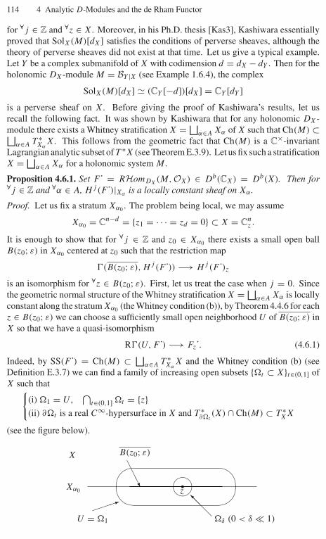
114 4 Analytic D-Modules and the de Rham Functor
for ∀j ∈ Z and ∀z ∈ X. Moreover, in his Ph.D. thesis [Kas3], Kashiwara essentiallyproved that SolX(M)[dX] satisfies the conditions of perverse sheaves, although thetheory of perverse sheaves did not exist at that time. Let us give a typical example.Let Y be a complex submanifold of X with codimension d = dX − dY . Then for theholonomic DX-module M = BY |X (see Example 1.6.4), the complex
SolX(M)[dX] � (CY [−d])[dX] = CY [dY ]is a perverse sheaf on X. Before giving the proof of Kashiwara’s results, let usrecall the following fact. It was shown by Kashiwara that for any holonomic DX-module there exists a Whitney stratification X = ⊔
α∈A Xα of X such that Ch(M) ⊂⊔α∈A T ∗
XαX. This follows from the geometric fact that Ch(M) is a C×-invariant
Lagrangian analytic subset of T ∗X (see Theorem E.3.9). Let us fix such a stratificationX = ⊔
α∈A Xα for a holonomic system M .
Proposition 4.6.1. Set F˙ = RHomDX(M, OX) ∈ Db(CX) = Db(X). Then for
∀j ∈ Z and ∀α ∈ A, Hj (F˙)|Xα is a locally constant sheaf on Xα .
Proof. Let us fix a stratum Xα0 . The problem being local, we may assume
Xα0 = Cn−d = {z1 = · · · = zd = 0} ⊂ X = Cnz .
It is enough to show that for ∀j ∈ Z and z0 ∈ Xα0 there exists a small open ballB(z0; ε) in Xα0 centered at z0 such that the restriction map
�(B(z0; ε), Hj (F˙)) −→ Hj (F˙)z
is an isomorphism for ∀z ∈ B(z0; ε). First, let us treat the case when j = 0. Sincethe geometric normal structure of the Whitney stratification X = ⊔
α∈A Xα is locallyconstant along the stratum Xα0 (the Whitney condition (b)), by Theorem 4.4.6 for eachz ∈ B(z0; ε) we can choose a sufficiently small open neighborhood U of B(z0; ε) inX so that we have a quasi-isomorphism
R�(U, F˙) −→ Fz . (4.6.1)
Indeed, by SS(F˙) = Ch(M) ⊂ ⊔α∈A T ∗
XαX and the Whitney condition (b) (see
Definition E.3.7) we can find a family of increasing open subsets {�t ⊂ X}t∈(0,1] ofX such that{
(i) �1 = U ,⋂
t∈(0,1] �t = {z}(ii) ∂�t is a real C∞-hypersurface in X and T ∗
∂�t(X) ∩ Ch(M) ⊂ T ∗
XX
(see the figure below).
����
����
��������
�
�
X
Xα0 z
�δ (0 < δ # 1)U = �1
B(z0; ε)
4.6 Kashiwara’s constructibility theorem 115
Since Hj (F˙) = 0 for j < 0, it follows from the quasi-isomorphism (4.6.1) that
�(U, H 0(F˙)) −→∼ H 0(F˙)z.
If we take an inductive limit of the left-hand side by shrinking U , we get the desiredisomorphism
�(B(z0; ε), H 0(F˙)) −→∼ H 0(F˙)z.
This shows that H 0(F˙)|Xα0is a locally constant sheaf on Xα0 in a neighborhood of
z0 ∈ Xα0 . To prove the corresponding assertion for H 1(F˙)|Xα0at the given point
z0 ∈ Xα , first choose a sufficiently small open ball B(z0; ε) in Xα0 centered at z0 sothat we have a quasi-isomorphism
R�(B(z0; ε), F˙) −→∼ Fz˙for ∀z ∈ B(z0; ε). Next setting K = B(z0; ε) and fixing z ∈ B(z0; ε) consider themorphism of distinguished triangles
R�(K, H 0(F˙)) −−−−→ R�(K, F˙) −−−−→ R�(K, τ�1F˙) +1−−−−→⏐⏐ �⏐⏐ ⏐⏐
H 0(F˙)z −−−−→ Fz˙ −−−−→ τ�1Fz˙ +1−−−−→ .
Then the leftmost vertical arrow is a quasi-isomorphism, because H 0(F˙)|Xα0is a
locally constant sheaf on Xα0 and K is contractible. Therefore, the rightmost verticalarrow is also a quasi-isomorphism:
R�(B(z0; ε), τ�1F˙) −→∼ τ�1Fz .
Taking H 1(•) of both sides, we finally get
�(B(z0; ε), H 1(F˙)) −→∼ H 1(F˙)z.
By repeating this argument, we can finally show that for all j ∈ Z, Hj (F˙)|Xα0is a
locally constant sheaf on Xα for ∀α ∈ A. This completes the proof. ��Proposition 4.6.2. Let M be a holonomic DX-module. Then for ∀j ∈ Z and ∀z ∈ X
the stalk Hj [RHomDX(M, OX)]z at z is a finite-dimensional vector space over C.
Proof. Let X = ⊔α∈A Xα be a Whitney stratification of X such that Ch(M) ⊂⊔
α∈A T ∗Xα
X. Let us prove our assertion for z ∈ Xα . By the Whitney condition (b)of the stratification
⊔α∈A Xα we can take a small positive number δ > 0 such that
T ∗∂(B(z;ε))X ∩ Ch(M) ⊂ T ∗
XX
for 0 < ∀ε < δ. Here B(z; ε) is an open ball in X centered at z with radius ε.Therefore, by the non-characteristic deformation lemma (see Theorem 4.4.6) we have

116 4 Analytic D-Modules and the de Rham Functor
R�(B(z; ε1), RHomDX(M, OX)) −→∼ R�(B(z; ε2), RHomDX
(M, OX))
for 0 < ∀ε2 < ∀ε1 < δ. Since the open balls B(z; εi) (i = 1, 2) are Stein, thisquasi-isomorphism can be represented by the morphism
0 −−−−→ OX(B(z; ε1))N0P1×−−−−→ OX(B(z; ε1))N1
P2×−−−−→ · · ·⏐⏐ ⏐⏐0 −−−−→ OX(B(z; ε2))N0
P1×−−−−→ OX(B(z; ε2))N1P2×−−−−→ · · ·
between complexes, where Pi is an Ni ×Ni−1 matrix of differential operators. Sincethe vertical arrows are compact maps of Fréchet spaces, the resulting cohomologygroups
Hi(B(z; ε1), RHomDX(M, OX)) −→∼ Hi(B(z; ε2), RHomDX
(M, OX))
are finite dimensional by a standard result in functional analysis. ��By Proposition 4.2.1, 4.6.1 and 4.6.2 we obtain Kashiwara’s constructibility the-
orem:
Theorem 4.6.3. Let M be a holonomic D-module on a complex manifold X. ThenSolX(M) = RHomDX
(M, OX) and DRX(M) = �X ⊗L
DX
M are objects in the
category Dbc (X).
For a holonomic DX-module M we saw that SolX(M)[dX] and DRX(M) wereconstructible sheaves on X. Next we will prove moreover that they are dual to eachother:
DRX(M) −→∼ DX(SolX(M)[dX]),where DX : Db
c (X) ∼→ Dbc (X) is the Verdier duality functor. For this purpose, recall
that for a point z ∈ X the complex R�{z}(OX)|z satisfies
Hj(R�{z}(OX)|z
) � 0 for ∀j = dX
and that B∞{z}|X = HdX(R�{z}(OX)|z) is an (FS) type (Fréchet–Schwartz type) topo-logical vector space. Regarding B∞{z}|X as the space of Sato’s hyperfunctions supportedby the point z ∈ X, we see that the (DFS) type (dual F-S type) topological vectorspace (OX)z is a topological dual of B∞{z}|X. The following results were also obtainedin Kashiwara [Kas3].
Proposition 4.6.4. Let M be a holonomic DX-module. Then
(i) For ∀z ∈ X and ∀i ∈ Z, ExtiDX
(M, B∞{z}|X) is a finite-dimensional vector spaceover C.
(ii) For ∀z ∈ X and ∀i ∈ Z, the vector spaces H−i (DRX(M)z) andExtiDX
(M, B∞{z}|X)
are dual to each other.
4.6 Kashiwara’s constructibility theorem 117
(iii) DRX(M) −→∼ DX(SolX(M)[dX]).Proof. (i) Since RHomDX
(M, B∞{z}|X) = R�{z}RHomDX(M, OX)[dX] and the func-
tor R�{z}(•) preserves the constructibility, the result follows.(ii) Let us take a locally free resolution
0 −→ DNk
X −→ · · · ×P2−−→ DN1X
×P1−−→ DN0X −→ M −→ 0
of M on an open neighborhood of z ∈ X, where Pi is a Ni×Ni−1 matrix of differentialoperators acting on the right of D
Ni
X . Then we get
DRX(M) = [0 −→ (�X)Nk −→ · · · ×P2−−→ (�X)N1
×P1−−→ (�X)N0 −→ 0],
RHomDX(M, B∞{z}|X)
= [0 −→ B∞{z}|X
N0 P1×−−→ B∞{z}|XN1 P2×−−→ · · · −→ B∞{z}|X
Nk −→ 0].
Taking a local coordinate and identifying �X with OX, we also have
DRX(M)z = [ · · · P ∗2 ×−−→ (OX)N1
z
P ∗1 ×−−→ (OX)N0
z −→ 0],
where P ∗i is a formal adjoint of Pi . Because (OX)z and B∞{z}|X are topological dual
to each other, and both DRX(M)z and RHomDX(M, B∞{z}|X) have finite-dimensional
cohomology groups, we obtain the duality isomorphism[H−i (DRX(M)z)
]∗ � ExtiDX
(M, B∞{z}|X).
(iii) Since CX � RHomDX(OX, OX), we have a natural morphism
DRX(M) = RHomDX(OX, M)[dX]
∃−→ RHomCX
(RHomDX
(M, OX), RHomDX(OX, OX)
)[dX]� RHomCX
(SolX(M)[dX], CX
)[2dX]� DX(SolX(M)[dX]).
Our task is to prove DRX(M)z � DX(SolX(M)[dX])z for ∀z ∈ X. Indeed, by (ii),we get the following chain of isomorphisms for i{z} : {z} ↪→ X:
DX(SolX(M)[dX])z = i−1{z} DX(SolX(M)[dX])
� D{pt}i!{z}(SolX(M)[dX])� [
RHomDX(M, R�{z}(OX)[dX])]∗
� [RHomDX
(M, B∞{z}|X)]∗
� DRX(M)z.
This completes the proof. ��
118 4 Analytic D-Modules and the de Rham Functor
Corollary 4.6.5. Let M be a holonomic DX-module and DXM its dual. Then wehave isomorphisms{
DX(DRX(M)) � DRX(DXM)
DX(SolX(M)[dX]) � SolX(DXM)[dX].Proof. The results follow immediately from Proposition 4.6.4 and the formulaDRX(DXM) � SolX(M)[dX]. ��Theorem 4.6.6. Let X be a complex manifold and M a holonomic D-module on it.Then SolX(M)[dX] = RHomDX
(M, OX)[dX] and DRX(M) = �X ⊗L
DX
M are
perverse sheaves on X.
Proof. By DRX(M) � SolX(DXM)[dX], it is sufficient to prove that F˙ =SolX(M)[dX] is a perverse sheaf for any holonomic DX-module M . Moreover, sincewe have DX(SolX(M)[dX]) � SolX(DXM)[dX] by Corollary 4.6.5, we have only toprove that dim supp(Hj (F˙)) ≤ −j for ∀j ∈ Z. Let us take a Whitney stratificationX = ⊔
α∈A Xα of X such that Ch(M) ⊂ ⊔α∈A T ∗
XαX and set iXα : Xα ↪−→ X for
α ∈ A. Then by Proposition 4.6.1 the complex i−1Xα
F˙ of sheaves on Xα has locally
constant cohomology groups for ∀α ∈ A. For j ∈ Z set Z = supp Hj (F˙). Then Z isa union of connected components of strata Xα’s. We need to prove dim Z = dZ ≤ −j .Choose a smooth point z of Z contained in a stratum Xα such that dim Xα = dim Z
and take a germ of complex submanifold Y of X at z which intersects with Z transver-sally at z ∈ Z (dim Y = dY = dX − dZ). We can choose the pair (z, Y ) so that Y isnon-characteristic for M , because for the Whitney stratification X = ⊔
α∈A Xα wehave the estimate Ch(M) ⊂ ⊔
α∈A T ∗Xα
X. Therefore, by the Cauchy–Kowalevski–Kashiwara theorem (Theorem 4.3.2), we obtain
F˙|Y = RHomDX(M, OX)|Y [dX]
� RHomDY(MY , OY )[dX].
Our assumption Hj (F˙)z = 0 implies Extj+dX
DY(MY , OY )z = 0. On the other hand,
by Theorem 4.1.2 and
RHomDY(MY , OY ) � RHomDY
(MY , DY ) ⊗L
DYOY ,
we have ExtiDY
(MY , OY ) = 0 for ∀i > dY . Hence we must have j + dX ≤ dY ⇐⇒dZ = dX − dY ≤ −j . This completes the proof. ��
Let M be a holonomic DX-module as before. Then Kashiwara’s constructibilitytheorem implies that for any point x ∈ X the local Euler–Poincaré index
χx[SolX(M)] :=∑i∈Z
(−1)i dim ExtiDX
(M, OX)x
of SolX(M) at x is a finite number (an integer). An important problem is to expressthis local Euler–Poincaré index in terms of geometric invariants of M . This problem
4.7 Analytic D-modules associated to algebraic D-modules 119
was solved by Kashiwara [Kas8] and its solution has many applications in variousfields of mathematics.
Let us briefly explain this result. First take a Whitney stratification X = ⊔α∈A Xα
of X such that Ch(M) ⊂ ⊔α∈A T ∗
XαX. Next denote by mα ∈ Z≥0 the multiplicity of
the coherent OT ∗X-module grF M = OT ∗X ⊗π−1 grF DXπ−1(grF M) along T ∗
XαX,
where F is a good filtration of M and π : T ∗X → X is the projection. Then thecharacteristic cycle CC(M) of the (analytic) holonomic DX-module M is defined by
CC(M) :=∑α∈A
mα[T ∗Xα
X].
This is a Lagrangian cycle in T ∗X. Finally, for an analytic subset S ⊂ X denoteby EuS : S → Z the Euler obstruction of S, which is introduced by Kashiwara[Kas2], [Kas8] and MacPherson [Mac] independently. Recall that for any Whitneystratification of S the Euler obstruction EuS is a locally constant function on eachstratum (and on the regular part of S, the value of EuS is one). Then we have
Theorem 4.6.7 (Kashiwara [Kas2], [Kas8]). For any x ∈ X the local Euler–Poincaré index χx[SolX(M)] of the solution complex SolX(M) at x is given by
χx[SolX(M)] =∑
x∈Xα
(−1)cα mα · EuXα(x),
where cα is the codimension of the stratum Xα in X.
Kashiwara’s local index theorem for holonomic D-modules was a starting pointof intensive activities in the last decades. The global index theorem was obtainedby Dubson [Du] and its generalization to real constructible sheaves was proved byKashiwara [Kas11] (see also Kashiwara–Schapira [KS2] for the details). As forfurther developments of the theory of index theorems, see, for example, [BMM],[Gi], [Gui], [SS], [SV], [Tk1]. Note also that Euler obstructions play a central role inthe study of characteristic classes of singular varieties (see [Mac], [Sab1]).
4.7 Analytic D-modules associated to algebraic D-modules
Recall that for an algebraic variety X we denote by Xan the corresponding analyticspace. We have a morphism ι = ιX : Xan → X of topological spaces, and amorphism ι−1OX → OXan of sheaves of rings. In other words we have a morphism(Xan, OXan ) → (X, OX) of ringed spaces.
Assume that X is a smooth algebraic variety. Then Xan is a complex manifold,and we have a canonical morphism
ι−1DX → DXan
of sheaves of rings satisfying
120 4 Analytic D-Modules and the de Rham Functor
DXan � OXan ⊗ι−1OXι−1DX � ι−1DX ⊗ι−1OX
OXan .
Hence we obtain a functor
(•)an : Mod(DX) → Mod(DXan )
sending M ∈ Mod(DX) to Man := DXan ⊗ι−1DXι−1M ∈ Mod(DXan ). Since DXan
is faithfully flat over ι−1DX, this functor is exact and extends to a functor
(•)an : Db(DX) → Db(DXan )
between derived categories. Note that (•)an induces
(•)an : Modc(DX) → Modc(DXan ), (•)an : Db(DX) → Db(DXan ).
We will sometimes write (M ·)an = DXan ⊗DXM · by abuse of notation.
The following is easily verified.
Proposition 4.7.1. For M · ∈ Dbc (DX) we have (DXM ·)an � DXan (M ·)an.
Proposition 4.7.2. Let f : X → Y be a morphism of smooth algebraic varieties.
(i) For M · ∈ Db(DY ) we have (f †M ·)an � (f an)†(M ·)an.(ii) For M · ∈ Db(DX) we have a canonical morphism (
∫f
M ·)an → ∫f an (M ·)an.
This morphism is an isomorphism if f is proper and M · ∈ Dbc (DX).
Proof. The proof of (i) is easy and omitted.Let us show (ii). First note that there exists a canonical morphism
(f an)−1DY an ⊗(f an)−1ι−1
Y DYι−1X DY←X → DY an←Xan .
Indeed, it is obtained by applying the side-changing operation to
ι−1X DX→Y ⊗
(f an)−1ι−1Y DY
(f an)−1DY an
= ι−1X OX ⊗
(f an)−1ι−1Y OY
(f an)−1DY an
�(ι−1X OX ⊗
(f an)−1ι−1Y OY
(f an)−1OY an
)⊗(f an)−1OY an (f an)−1DY an
→ OXan ⊗(f an)−1OY an (f an)−1DY an
= DXan→Y an
(note ιY ◦ f an = f ◦ ιX). Next note that there exists a canonical morphism
ι−1Y Rf∗K · → Rf an∗ ι−1
X K ·
for any K · ∈ Db(f −1DY ). Indeed, it is obtained as the image of Id for
Homι−1X f −1DY
(ι−1X K ·, ι−1
X K ·) � Homf −1DY(K ·, RιX∗ι−1
X K ·)

4.7 Analytic D-modules associated to algebraic D-modules 121
→ HomDY(Rf∗K ·, Rf∗RιX∗ι−1
X K ·)� HomDY
(Rf∗K ·, RιY∗Rf an∗ ι−1X K ·)
� Homι−1Y DY
(ι−1Y Rf∗K ·, Rf an∗ ι−1
X K ·).
Then we obtain(∫f
M ·)an = DY an ⊗ι−1Y DY
ι−1Y Rf∗(DY←X ⊗L
DXM ·)
→ DY an ⊗ι−1Y DY
Rf an∗ ι−1X (DY←X ⊗L
DXM ·)
→ Rf an∗(
(f an)−1DY an ⊗L
(f an)−1ι−1Y DY
ι−1X DY←X ⊗L
ι−1X DX
ι−1X M ·
)→ Rf an∗
(DY an←Xan ⊗L
ι−1X DX
ι−1X M ·
)→ Rf an∗
(DY an←Xan ⊗L
DXan DXan ⊗L
ι−1X DX
ι−1X M ·
)=∫
f an(M ·)an.
It remains to show that (∫
fM ·)an → ∫
f an (M ·)an is an isomorphism if f is proper. Wemay assume that f is either a closed embedding or a projection f : X = Y ×Pn → Y .The case of a closed embedding is easy and omitted. Assume that f is a projectionf : X = Y × Pn → Y . We may also assume that M · = M ∈ Modc(DX). In thiscase we have (∫
f
M)an = OY an ⊗
ι−1Y OY
Rf∗(DRX/Y (M)),∫f an
Man = Rf an∗ (DRXan/Y an (Man)),
and hence it is sufficient to show that
OY an ⊗ι−1Y OY
Rf∗(DRX/Y (M)k) � Rf an∗ (DRXan/Y an (Man)k)
for each k. Since DRX/Y (M)k is a quasi-coherent OX-module satisfying
OXan ⊗ι−1X OX
DRX/Y (M)k � DRXan/Y an (Man)k,
this follows from the GAGA-principle. ��For a smooth algebraic variety X we define functors
DRX : Db(DX) −→ Db(CXan ),
SolX : Db(DX) −→ Db(CXan )op
122 4 Analytic D-Modules and the de Rham Functor
by
DRX(M ·) := DRXan ((M ·)an) = �Xan ⊗LDXan (M ·)an,
SolX(M ·) := SolXan ((M ·)an) = RHomDXan ((M ·)an, OXan ).
Remark 4.7.3. It is not a good idea to consider �X ⊗LDX
M · and RHomDX(OX, M ·)
for a smooth algebraic variety X as the following example suggests. Regard X = Cas an algebraic variety, and set M = DX/DX( d
dx− λ) for λ ∈ C \ Z. Then we
easily see that DRX(M) � CXan [1] and SolX(M) � CXan , while �X ⊗LDX
M =RHomDX
(OX, M)[1] = 0. This comes from the fact that the differential equationdudx
= λu has a holomorphic solution exp(λx) ∈ OXan which does not belong to OX.
By Proposition 4.2.1 and Proposition 4.7.1 we have the following.
Proposition 4.7.4. Let X be a smooth algebraic variety. For M · ∈ Dbc (DX) we have
DRX(M ·) � RHomDXan (OXan , (M ·)an)[dX] � SolX(DXM ·)[dX].By Theorem 4.2.5 and Proposition 4.7.2 we have the following.
Proposition 4.7.5. Let f : X → Y be a morphism of smooth algebraic varieties.For M · ∈ Db
c (DX) there exists a canonical morphism
DRY (
∫f
M) → Rf∗(DRX(M ·)).
This morphism is an isomorphism if f is proper.
By Corollary 4.3.3 and Proposition 4.7.2 we have the following.
Proposition 4.7.6. Let f : X → Y be a morphism of smooth algebraic varieties.Assume that f is non-characteristic for a coherent DY -module M . Then we have
DRX(Lf ∗M) � f −1 DRY (M)[dX − dY ].The following is a special case of Kashiwara’s constructibility theorem for analytic
holonomic D-modules. Here we present another proof following Bernstein [Ber3]for the convenience of readers who wants a shortcut for algebraic D-modules.
Theorem 4.7.7. For M · ∈ Dbh(DX) we have DRX(M ·), SolX(M ·) ∈ Db
c (X).
Proof. By Proposition 4.7.4 we have only to show the assertion on DRX(M ·). More-over, we may assume that M · = M ∈ Modh(DX). By Proposition 3.1.6 M isgenerically an integrable connection, and hence DRX(M) is generically a local sys-tem up to a shift of degrees. Hence there exists an open dense subset U of X suchthat DRU (M|U ) ∈ Db
c (U). Therefore, it is sufficient to show the following.
Claim. Let M ∈ Modh(DX), and assume that DRU (M|U ) ∈ Dbc (U) for an open
dense subset U of X. Then there exists an open dense subset Y of X \ U such thatDRU∪Y (M|U∪Y ) ∈ Db
c (U ∪ Y ).
4.7 Analytic D-modules associated to algebraic D-modules 123
For each irreducible component Z of X\U there exists an étale morphism f froman open subset V of X onto an open subset V ′ of An such that V ∩ (X \ U) (resp.V ′∩An−k) is an open dense subset of Z (resp. An−k) and f −1(V ′∩An−k) = V ∩(X\U), where 0 < k ≤ n and An−k is identified with the subset {0} × An−k of An (seeTheorem A.5.3). Since f is an étale morphism, DRV (M|V ) ∈ Db
c (V ) if and only if
f∗(DRV (M|V )) ∈ Dbc (V ′). Moreover, we have f∗(DRV (M|V )) = DRV ′(
∫ 0f
(M|V ))
by Proposition 4.7.5. Hence we may assume from the beginning that X is an opensubset of An, X\U = X∩An−k , and X∩An−k is dense in An−k . Set T = X∩An−k .By shrinking X if necessary we may assume that X is an open subset of Ak × T .
Now we regard Ak as an open subset of Pk . Set S = (Pk ×T )\X. Then we havePk × T = S � U � T , X = U � T , and S and T are closed subsets of Pk × T . Letp : Pk × T → T be the projection and let jX : X → Pk × T , jU : U → Pk × T ,jS : S → Pk × T , jT : T → Pk × T be the embeddings. Set N · = ∫
jXM ,
K · = DRPk×T (N ·). By applying Rp∗(= Rp!) to the distinguished triangle
jU !j−1U K · −→ K · −→ jS!j−1
S K · ⊕ jT !j−1T K · +1−→
we obtain a distinguished triangle
R(p ◦ jU )!j−1U K · −→ Rp∗K · −→ R(p ◦ jS)!j−1
S K · ⊕ R(p ◦ jT )!j−1T K · +1−→ .
By j−1U K · � DRU (M|U ) ∈ Db
c (U) we have R(p ◦ jU )!j−1U K · ∈ Db
c (T ). ByProposition 4.7.5 we have
Rp∗K · = Rp∗ DRPk×T (N ·) � DRT (
∫p
N ·).
By∫
pN · ∈ Db
h(DT ) there exists an open dense subset Y of T such that Rp∗K ·|Y an ∈Db
c (Y ). It follows from the above distinguished triangle that R(p ◦ jT )!j−1T K ·|Y an ∈
Dbc (Y ). By p ◦ jT = id we have R(p ◦ jT )!j−1
T K · � i−1 DRX(M), wherei : T → X is the embedding. Thus i−1 DRX(M)|Y an ∈ Db
c (Y ). Hence we haveDRU∪Y (M|U∪Y ) ∈ Db
c (U ∪ Y ). The proof is complete. ��The technique used in the proof of Theorem 4.7.7 also allows us to prove the
following results.
Proposition 4.7.8. Let X and Y be smooth algebraic varieties. For M · ∈ Dbc (DX)
and N · ∈ Dbc (DY ) we have a canonical morphism
DRX(M ·) �C DRY (N ·) → DRX×Y (M · � N ·).
This morphism is an isomorphism if M · ∈ Dbh(DX) or N · ∈ Db
h(DY ).
Proposition 4.7.9. Let X be a smooth algebraic variety. For M · ∈ Dbc (DX) we have
canonical morphisms
124 4 Analytic D-Modules and the de Rham Functor
DRX(DXM ·) → DX(DRX(M ·)),SolX(DXM ·)[dX] → DX(SolX(M ·)[dX]).
These morphisms are isomorphisms if M · ∈ Dbh(DX).
Proof of Proposition 4.7.8. Let M · ∈ Dbc (DX) and N · ∈ Db
c (DX). By
(M · � N ·)an � DXan×Y an ⊗LDXan �CDY an
((M ·)an �C (N ·)an)
we have
DRX×Y (M · � N ·) � �Xan×Y an ⊗LDXan �CDY an
((M ·)an �C (N ·)an).
On the other hand we have
DRX(M ·) �C DRY (N ·) � (�Xan ⊗LDXan (M ·)an) �C (�Y an ⊗L
DY an (N ·)an)
� (�Xan �C �Y an ) ⊗LDXan �CDY an
((M ·)an �C (N ·)an).
Hence the canonical morphism �Xan �C �Y an → �Xan×Y an induces a canonicalmorphism
DRX(M ·) �C DRY (N ·) → DRX×Y (M · � N ·).
Let us show that this morphism is an isomorphism if either M · ∈ Dbh(DX) or
N · ∈ Dbh(DY ). By symmetry we can only deal with the case M · ∈ Db
h(DX).We first show it when M · is an integrable connection. In this case we have
(M ·)an � OXan ⊗CXan K for a local system K on Xan and we have DRX(M ·) �K[dX]. Then we have
(M · � N ·)an � p−11 K ⊗CXan×Y an (OX � N ·)an � p−1
1 K ⊗CXan×Y an (p∗2N ·)an,
where p1 : X × Y → X and p2 : X × Y → Y are projections. Hence we have
DRX×Y (M · � N ·) � p−11 K ⊗CXan×Y an DRX×Y (p∗
2N ·)� p−1
1 K ⊗CXan×Y an p−12 DRY (N ·)[dX]
� DRX(M ·) �C DRY (N ·)
by Proposition 4.7.6.Finally, we consider the general case. We may assume that M · = M ∈
Modh(DX). Since M is generically an integrable connection, there exists an opensubset U of X such that the canonical morphism
DRU (M|U ) �C DRY (N ·) → DRU×Y ((M|U ) � N ·)
is an isomorphism. Therefore, it is sufficient to show the following.
4.7 Analytic D-modules associated to algebraic D-modules 125
Claim. Assume that the canonical morphism
DRU (M|U ) �C DRY (N ·) → DRU×Y ((M|U ) � N ·)
is an isomorphism for an open dense subset U of X. Then there exists an open densesubset Z of X \ U such that
DRU∪Z(M|U∪Z) �C DRY (N ·) → DR(U∪Z)×Y ((M|U∪Z) � N ·)
is an isomorphism.
This can be proved similarly to the claim in Theorem 4.7.7. The details areomitted. ��Proof of Proposition 4.7.9. By Proposition 4.7.4 it is sufficient to show that thereexists a canonical morphism
SolX(M ·) → DX(DRX(M ·))[−dX] (M · ∈ Dbc (DX)),
which turns out to be an isomorphism for M · ∈ Dbh(DX).
Let M · ∈ Dbc (DX). Then we have a canonical morphism
RHomDXan (OXan , (M ·)an) ⊗CXan RHomDXan ((M ·)an, OXan )
→ RHomDXan (OXan , OXan ).
By
RHomDXan (OXan , (M ·)an) � DRX(M)[−dX],RHomDXan ((M ·)an, OXan ) � SolX(M),
RHomDXan (OXan , OXan ) � CXan ,
we obtainDRX(M) ⊗CXan SolX(M) → CXan [dX].
Hence there exists a canonical morphism
SolX(M) → RHomCXan (DRX(M), CXan [dX])(� DX(DRX(M ·))[−dX]).
Let us show that this morphism is an isomorphism for M · ∈ Dbh(DX). We
may assume that M · = M ∈ Modh(DX). If M is an integrable connection, thenwe have Man � OXan ⊗CXan K for a local system K on Xan, and SolX(M) �HomCXan (K, CXan ), DRX(M) � K[dX]. Hence the assertion is obvious in thiscase. Let us consider the general case M ∈ Modh(DX). Since M is generically anintegrable connection, there exists an open subset U of X such that the canonicalmorphism
SolU (M ·|U ) → DU (DRU (M ·|U ))[−dX]is an isomorphism. Therefore, it is sufficient to show the following.
126 4 Analytic D-Modules and the de Rham Functor
Claim. Assume that the canonical morphism
SolU (M ·|U ) → DU (DRU (M ·|U ))[−dX]is an isomorphism for an open dense subset U of X. Then there exists an open densesubset Y of X \ U such that
SolU∪Y (M ·|U∪Y ) → DU∪Y (DRU∪Y (M ·|U∪Y ))[−dX]is an isomorphism.
This can be proved similarly to the claim in Theorem 4.7.7. Details are omitted.��
5
Theory of Meromorphic Connections
In this chapter we present several important results on meromorphic connections suchas the Riemann–Hilbert correspondence for regular meromorphic connections due toDeligne. In subsequent chapters these results will be effectively used to establishvarious properties of regular holonomic systems.
5.1 Meromorphic connections in the one-dimensional case
5.1.1 Systems of ODEs and meromorphic connections
We start from the classical theory of ordinary differential equations (we call themODEs for short). We always consider the problem in an open neighborhood ofx = 0 ∈ C. Here the complex plane C is considered as a complex manifold and weuse only the classical topology in this subsection and the next. Set O = (OC)0 anddenote by K its quotient field. Then K is the field of meromorphic functions withpossible poles at x = 0. Note that O and K are identified with the ring of convergentpower series C{{x}} at x = 0 and its quotient field C{{x}}[x−1], respectively.
For a matrix A(x) = (aij (x)) ∈ Mn(K) let us consider the system of ODEs
d
dx
→u (x) = A(x)
→u (x), (5.1.1)
where→u (x) = t (u1(x), u2(x), . . . , un(x)) is a column vector of unknown functions.
Setting→v (x) = T −1→
u (x) for an invertible matrix T = T (x) ∈ GLn(K) (5.1.1) isrewritten as
d
dx
→v (x) =
(T −1AT − T −1 d
dxT)→
v (x).
Therefore, we say that two systems
d
dx
→u (x) = A(x)
→u (x) (A(x) ∈ Mn(K))
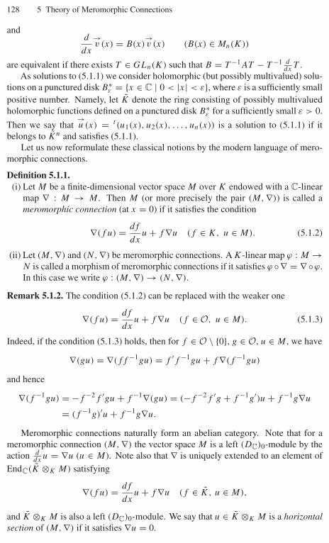
128 5 Theory of Meromorphic Connections
andd
dx
→v (x) = B(x)
→v (x) (B(x) ∈ Mn(K))
are equivalent if there exists T ∈ GLn(K) such that B = T −1AT − T −1 ddx
T .As solutions to (5.1.1) we consider holomorphic (but possibly multivalued) solu-
tions on a punctured disk B∗ε = {x ∈ C | 0 < |x| < ε}, where ε is a sufficiently small
positive number. Namely, let K denote the ring consisting of possibly multivaluedholomorphic functions defined on a punctured disk B∗
ε for a sufficiently small ε > 0.
Then we say that→u (x) = t (u1(x), u2(x), . . . , un(x)) is a solution to (5.1.1) if it
belongs to Kn and satisfies (5.1.1).Let us now reformulate these classical notions by the modern language of mero-
morphic connections.
Definition 5.1.1.(i) Let M be a finite-dimensional vector space M over K endowed with a C-linear
map ∇ : M → M . Then M (or more precisely the pair (M, ∇)) is called ameromorphic connection (at x = 0) if it satisfies the condition
∇(f u) = df
dxu + f ∇u (f ∈ K, u ∈ M). (5.1.2)
(ii) Let (M, ∇) and (N, ∇) be meromorphic connections. A K-linear map ϕ : M →N is called a morphism of meromorphic connections if it satisfies ϕ ◦∇ = ∇ ◦ϕ.In this case we write ϕ : (M, ∇) → (N, ∇).
Remark 5.1.2. The condition (5.1.2) can be replaced with the weaker one
∇(f u) = df
dxu + f ∇u (f ∈ O, u ∈ M). (5.1.3)
Indeed, if the condition (5.1.3) holds, then for f ∈ O \ {0}, g ∈ O, u ∈ M , we have
∇(gu) = ∇(ff −1gu) = f ′f −1gu + f ∇(f −1gu)
and hence
∇(f −1gu) = −f −2f ′gu + f −1∇(gu) = (−f −2f ′g + f −1g′)u + f −1g∇u
= (f −1g)′u + f −1g∇u.
Meromorphic connections naturally form an abelian category. Note that for ameromorphic connection (M, ∇) the vector space M is a left (DC)0-module by theaction d
dxu = ∇u (u ∈ M). Note also that ∇ is uniquely extended to an element of
EndC(K ⊗K M) satisfying
∇(f u) = df
dxu + f ∇u (f ∈ K, u ∈ M),
and K ⊗K M is also a left (DC)0-module. We say that u ∈ K ⊗K M is a horizontalsection of (M, ∇) if it satisfies ∇u = 0.
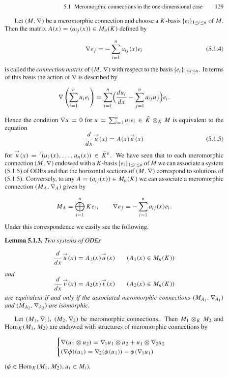
5.1 Meromorphic connections in the one-dimensional case 129
Let (M, ∇) be a meromorphic connection and choose a K-basis {ei}1≤i≤n of M .Then the matrix A(x) = (aij (x)) ∈ Mn(K) defined by
∇ej = −n∑
i=1
aij (x)ei (5.1.4)
is called the connection matrix of (M, ∇) with respect to the basis {ei}1≤i≤n. In termsof this basis the action of ∇ is described by
∇(
n∑i=1
uiei
)=
n∑i=1
(dui
dx−
n∑j=1
aij uj
)ei .
Hence the condition ∇u = 0 for u = ∑ni=1 uiei ∈ K ⊗K M is equivalent to the
equationd
dx
→u (x) = A(x)
→u (x) (5.1.5)
for→u (x) = t (u1(x), . . . , un(x)) ∈ Kn. We have seen that to each meromorphic
connection (M, ∇) endowed with a K-basis {ei}1≤i≤n of M we can associate a system(5.1.5) of ODEs and that the horizontal sections of (M, ∇) correspond to solutions of(5.1.5). Conversely, to any A = (aij (x)) ∈ Mn(K) we can associate a meromorphicconnection (MA, ∇A) given by
MA =n⊕
i=1
Kei, ∇ej = −n∑
i=1
aij (x)ei .
Under this correspondence we easily see the following.
Lemma 5.1.3. Two systems of ODEs
d
dx
→u (x) = A1(x)
→u (x) (A1(x) ∈ Mn(K))
andd
dx
→v (x) = A2(x)
→v (x) (A2(x) ∈ Mn(K))
are equivalent if and only if the associated meromorphic connections (MA1 , ∇A1)
and (MA2 , ∇A2) are isomorphic.
Let (M1, ∇1), (M2, ∇2) be meromorphic connections. Then M1 ⊗K M2 andHomK(M1, M2) are endowed with structures of meromorphic connections by{
∇(u1 ⊗ u2) = ∇1u1 ⊗ u2 + u1 ⊗ ∇2u2
(∇φ)(u1) = ∇2(φ(u1)) − φ(∇1u1)
(φ ∈ HomK(M1, M2), ui ∈ Mi).
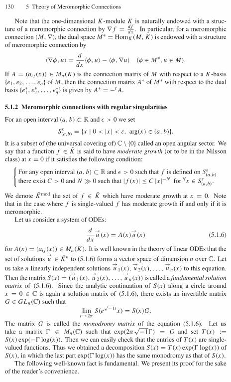
130 5 Theory of Meromorphic Connections
Note that the one-dimensional K-module K is naturally endowed with a struc-ture of a meromorphic connection by ∇f = df
dx. In particular, for a meromorphic
connection (M, ∇), the dual space M∗ = HomK(M, K) is endowed with a structureof meromorphic connection by
〈∇φ, u〉 = d
dx〈φ, u〉 − 〈φ, ∇u〉 (φ ∈ M∗, u ∈ M).
If A = (aij (x)) ∈ Mn(K) is the connection matrix of M with respect to a K-basis{e1, e2, . . . , en} of M , then the connection matrix A∗ of M∗ with respect to the dualbasis {e∗
1, e∗2, . . . , e∗
n} is given by A∗ = −tA.
5.1.2 Meromorphic connections with regular singularities
For an open interval (a, b) ⊂ R and ε > 0 we set
Sε(a,b) = {x | 0 < |x| < ε, arg(x) ∈ (a, b)}.
It is a subset of (the universal covering of) C \ {0} called an open angular sector. Wesay that a function f ∈ K is said to have moderate growth (or to be in the Nilssonclass) at x = 0 if it satisfies the following condition:{
For any open interval (a, b) ⊂ R and ε > 0 such that f is defined on Sε(a,b)
there exist C > 0 and N � 0 such that |f (x)| ≤ C |x|−N for ∀x ∈ Sε(a,b).
We denote Kmod the set of f ∈ K which have moderate growth at x = 0. Notethat in the case where f is single-valued f has moderate growth if and only if it ismeromorphic.
Let us consider a system of ODEs:
d
dx
→u (x) = A(x)
→u (x) (5.1.6)
for A(x) = (aij (x)) ∈ Mn(K). It is well known in the theory of linear ODEs that the
set of solutions→u ∈ Kn to (5.1.6) forms a vector space of dimension n over C. Let
us take n linearly independent solutions→u 1(x),
→u 2(x), . . . ,
→u n(x) to this equation.
Then the matrix S(x) = (→u 1(x),
→u 2(x), . . . ,
→u n(x)) is called a fundamental solution
matrix of (5.1.6). Since the analytic continuation of S(x) along a circle aroundx = 0 ∈ C is again a solution matrix of (5.1.6), there exists an invertible matrixG ∈ GLn(C) such that
limt→2π
S(e√−1t x) = S(x)G.
The matrix G is called the monodromy matrix of the equation (5.1.6). Let ustake a matrix � ∈ Mn(C) such that exp(2π
√−1�) = G and set T (x) :=S(x) exp(−� log(x)). Then we can easily check that the entries of T (x) are single-valued functions. Thus we obtained a decomposition S(x) = T (x) exp(� log(x)) ofS(x), in which the last part exp(� log(x)) has the same monodromy as that of S(x).
The following well-known fact is fundamental. We present its proof for the sakeof the reader’s convenience.
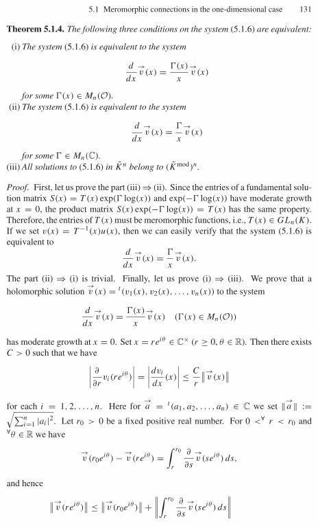
5.1 Meromorphic connections in the one-dimensional case 131
Theorem 5.1.4. The following three conditions on the system (5.1.6) are equivalent:
(i) The system (5.1.6) is equivalent to the system
d
dx
→v (x) = �(x)
x
→v (x)
for some �(x) ∈ Mn(O).(ii) The system (5.1.6) is equivalent to the system
d
dx
→v (x) = �
x
→v (x)
for some � ∈ Mn(C).(iii) All solutions to (5.1.6) in Kn belong to (Kmod)n.
Proof. First, let us prove the part (iii) ⇒ (ii). Since the entries of a fundamental solu-tion matrix S(x) = T (x) exp(� log(x)) and exp(−� log(x)) have moderate growthat x = 0, the product matrix S(x) exp(−� log(x)) = T (x) has the same property.Therefore, the entries of T (x) must be meromorphic functions, i.e., T (x) ∈ GLn(K).If we set v(x) = T −1(x)u(x), then we can easily verify that the system (5.1.6) isequivalent to
d
dx
→v (x) = �
x
→v (x).
The part (ii) ⇒ (i) is trivial. Finally, let us prove (i) ⇒ (iii). We prove that a
holomorphic solution→v (x) = t (v1(x), v2(x), . . . , vn(x)) to the system
d
dx
→v (x) = �(x)
x
→v (x) (�(x) ∈ Mn(O))
has moderate growth at x = 0. Set x = reiθ ∈ C× (r ≥ 0, θ ∈ R). Then there existsC > 0 such that we have∣∣∣∣ ∂
∂rvi(reiθ )
∣∣∣∣ =∣∣∣∣dvi
dx(x)
∣∣∣∣ ≤ C
r
∥∥→v (x)
∥∥for each i = 1, 2, . . . , n. Here for
→a = t (a1, a2, . . . , an) ∈ C we set ‖→
a ‖ :=√∑ni=1 |ai |2. Let r0 > 0 be a fixed positive real number. For 0 <∀ r < r0 and
∀θ ∈ R we have
→v (r0eiθ ) − →
v (reiθ ) =∫ r0
r
∂
∂s
→v (seiθ ) ds,
and hence ∥∥→v (reiθ )
∥∥ ≤ ∥∥→v (r0eiθ )
∥∥+∥∥∥∥∫ r0
r
∂
∂s
→v (seiθ ) ds
∥∥∥∥
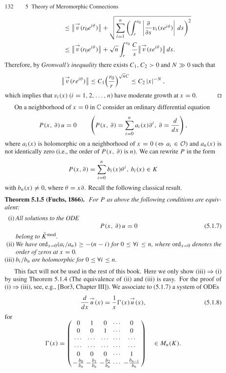
132 5 Theory of Meromorphic Connections
≤ ∥∥→v (r0eiθ )
∥∥+√√√√ n∑
i=1
(∫ r0
r
∣∣∣∣ ∂
∂svi(seiθ )
∣∣∣∣ ds
)2
≤ ∥∥→v (r0eiθ )
∥∥+ √n
∫ r0
r
C
s
∥∥→v (seiθ )
∥∥ ds.
Therefore, by Gronwall’s inequality there exists C1, C2 > 0 and N � 0 such that∥∥→v (reiθ )
∥∥ ≤ C1
( r0
r
)√nC ≤ C2 |x|−N ,
which implies that vi(x) (i = 1, 2, . . . , n) have moderate growth at x = 0. ��On a neighborhood of x = 0 in C consider an ordinary differential equation
P(x, ∂) u = 0
(P(x, ∂) =
n∑i=0
ai(x)∂i, ∂ = d
dx
),
where ai(x) is holomorphic on a neighborhood of x = 0 (⇔ ai ∈ O) and an(x) isnot identically zero (i.e., the order of P(x, ∂) is n). We can rewrite P in the form
P(x, ∂) =n∑
i=0
bi(x)θ i, bi(x) ∈ K
with bn(x) = 0, where θ = x∂ . Recall the following classical result.
Theorem 5.1.5 (Fuchs, 1866). For P as above the following conditions are equiv-alent:
(i) All solutions to the ODEP(x, ∂) u = 0 (5.1.7)
belong to Kmod .(ii) We have ordx=0(ai/an) ≥ −(n − i) for 0 ≤ ∀i ≤ n, where ordx=0 denotes the
order of zeros at x = 0.(iii) bi/bn are holomorphic for 0 ≤ ∀i ≤ n.
This fact will not be used in the rest of this book. Here we only show (iii) ⇒ (i)by using Theorem 5.1.4 (The equivalence of (ii) and (iii) is easy. For the proof of(i) ⇒ (iii), see, e.g., [Bor3, Chapter III]). We associate to (5.1.7) a system of ODEs
d
dx
→u (x) = 1
x�(x)
→u (x), (5.1.8)
for
�(x) =
⎛⎜⎜⎜⎜⎜⎜⎝
0 1 0 · · · 00 0 1 · · · 0
· · · · · · · · · · · · · · ·· · · · · · · · · · · · · · ·0 0 0 · · · 1
− b0bn
− b1bn
− b2bn
· · · − bn−1bn
⎞⎟⎟⎟⎟⎟⎟⎠ ∈ Mn(K).

5.1 Meromorphic connections in the one-dimensional case 133
Then u is a solution to (5.1.7) if and only if→u = t (u, θu, θ2u, . . . , θn−1u) is a
solution to (5.1.8). Since bi/bn are holomorphic, we see by Theorem 5.1.4 that anysolution u to (5.1.7) belongs to Kmod. The proof of (iii) ⇒ (i) is complete.
Definition 5.1.6. We say that a meromorphic connection (M, ∇) at x = 0 is regularif there exists a finitely generated O-submodule L ⊂ M which is stable by the actionof θ = x∇ (i.e., θL ⊂ L) and generates M over K . We call such an O-submodule L
an O-lattice of (M, ∇).
Lemma 5.1.7. Let (M, ∇) be a regular meromorphic connection. Then any O-latticeL of (M, ∇) is a free O-module of rank dimK M .
Proof. Since L is a torsion free finitely generated module over the principal idealdomain O, it is free of finite-rank. Hence it is sufficient to show that the canonicalhomomorphism K ⊗O L → M is an isomorphism. The surjectivity is clear. To showthe injectivity take a free basis {ei}1≤i≤n of L. It is sufficient to show that {ei}1≤i≤n
is linearly independent over K . Assume∑n
i=1 fiei = 0 for fi ∈ K . For N � 0 wehave ai := xNfi ∈ O for any i = 1, . . . , n. Then from
∑ni=1 aiei = 0 we obtain
ai = 0, and hence fi = 0. ��By this lemma we easily see that a meromorphic connection (M, ∇) is regular if
and only if there exists a K-basis {ei}1≤i≤n of M such that the associated system ofODEs is of the form
d
dx
→u (x) = �(x)
x
→u (x) (�(x) ∈ Mn(O)).
In particular, we have the following by Theorem 5.1.4.
Proposition 5.1.8. A meromorphic connection (M, ∇) is regular if and only if all ofits horizontal sections belong to Kmod ⊗K M .
Proposition 5.1.9. For a meromorphic connection (M, ∇) at x = 0, the followingthree conditions are equivalent:
(i) (M, ∇) is regular.(ii) For any u ∈ M there exists a finitely generated O-submodule L of M such
that u ∈ L and θL ⊂ L, i.e., M is a union of θ -stable finitely generated O-submodules.
(iii) For any u ∈ M there exists a polynomial
F(t) = tm + a1tm−1 + · · · + am ∈ O[t]such that F(θ)u = 0.
Proof. (i) ⇒ (ii): Let L ⊂ M be an O-lattice of (M, ∇). Then M = ⋃N≥0 x−NL
and each x−NL is a θ -stable finitely generated O-submodule of M .(ii) ⇒ (i): Take a K-basis e1, e2, . . . , en of M and choose a family of θ -stable
finitely generated O-submodules Li of M such that ei ∈ Li . Then the sum L =∑ni=1 Li ⊂ M is an O-lattice of (M, ∇).
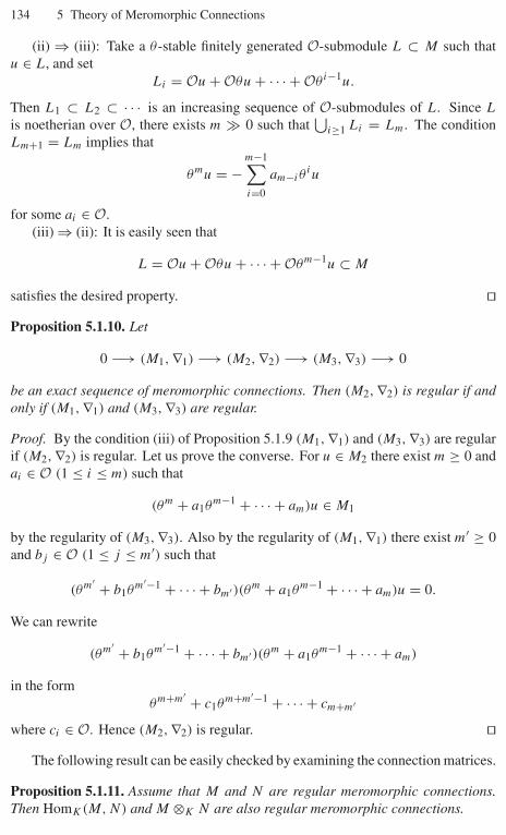
134 5 Theory of Meromorphic Connections
(ii) ⇒ (iii): Take a θ -stable finitely generated O-submodule L ⊂ M such thatu ∈ L, and set
Li = Ou + Oθu + · · · + Oθi−1u.
Then L1 ⊂ L2 ⊂ · · · is an increasing sequence of O-submodules of L. Since L
is noetherian over O, there exists m � 0 such that⋃
i≥1 Li = Lm. The conditionLm+1 = Lm implies that
θmu = −m−1∑i=0
am−iθiu
for some ai ∈ O.(iii) ⇒ (ii): It is easily seen that
L = Ou + Oθu + · · · + Oθm−1u ⊂ M
satisfies the desired property. ��Proposition 5.1.10. Let
0 −→ (M1, ∇1) −→ (M2, ∇2) −→ (M3, ∇3) −→ 0
be an exact sequence of meromorphic connections. Then (M2, ∇2) is regular if andonly if (M1, ∇1) and (M3, ∇3) are regular.
Proof. By the condition (iii) of Proposition 5.1.9 (M1, ∇1) and (M3, ∇3) are regularif (M2, ∇2) is regular. Let us prove the converse. For u ∈ M2 there exist m ≥ 0 andai ∈ O (1 ≤ i ≤ m) such that
(θm + a1θm−1 + · · · + am)u ∈ M1
by the regularity of (M3, ∇3). Also by the regularity of (M1, ∇1) there exist m′ ≥ 0and bj ∈ O (1 ≤ j ≤ m′) such that
(θm′ + b1θm′−1 + · · · + bm′)(θm + a1θm−1 + · · · + am)u = 0.
We can rewrite
(θm′ + b1θm′−1 + · · · + bm′)(θm + a1θm−1 + · · · + am)
in the formθm+m′ + c1θm+m′−1 + · · · + cm+m′
where ci ∈ O. Hence (M2, ∇2) is regular. ��The following result can be easily checked by examining the connection matrices.
Proposition 5.1.11. Assume that M and N are regular meromorphic connections.Then HomK(M, N) and M ⊗K N are also regular meromorphic connections.
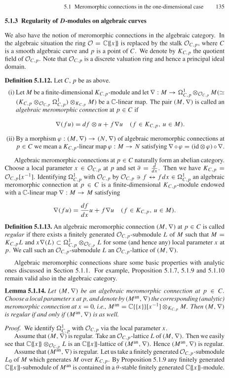
5.1 Meromorphic connections in the one-dimensional case 135
5.1.3 Regularity of D-modules on algebraic curves
We also have the notion of meromorphic connections in the algebraic category. Inthe algebraic situation the ring O = C{{x}} is replaced by the stalk OC,p, where C
is a smooth algebraic curve and p is a point of C. We denote by KC,p the quotientfield of OC,p. Note that OC,p is a discrete valuation ring and hence a principal idealdomain.
Definition 5.1.12. Let C, p be as above.
(i) Let M be a finite-dimensional KC,p-module and let ∇ : M → �1C,p ⊗OC,p
M(�(KC,p ⊗OC,p
�1C,p) ⊗KC,p
M) be a C-linear map. The pair (M, ∇) is called analgebraic meromorphic connection at p ∈ C if
∇(f u) = df ⊗ u + f ∇u (f ∈ KC,p, u ∈ M).
(ii) By a morphism ϕ : (M, ∇) → (N, ∇) of algebraic meromorphic connections atp ∈ C we mean a KC,p-linear map ϕ : M → N satisfying ∇ ◦ϕ = (id ⊗ϕ)◦∇.
Algebraic meromorphic connections at p ∈ C naturally form an abelian category.Choose a local parameter x ∈ OC,p at p and set ∂ = d
dx. Then we have KC,p =
OC,p[x−1]. Identifying �1C,p with OC,p by OC,p f ↔ f dx ∈ �1
C,p an algebraicmeromorphic connection at p ∈ C is a finite-dimensional KC,p-module endowedwith a C-linear map ∇ : M → M satisfying
∇(f u) = df
dxu + f ∇u (f ∈ KC,p, u ∈ M).
Definition 5.1.13. An algebraic meromorphic connection (M, ∇) at p ∈ C is calledregular if there exists a finitely generated OC,p-submodule L of M such that M =KC,pL and x∇(L) ⊂ �1
C,p ⊗OC,pL for some (and hence any) local parameter x at
p. We call such an OC,p-submodule L an OC,p-lattice of (M, ∇).
Algebraic meromorphic connections share some basic properties with analyticones discussed in Section 5.1.1. For example, Proposition 5.1.7, 5.1.9 and 5.1.10remain valid also in the algebraic category.
Lemma 5.1.14. Let (M, ∇) be an algebraic meromorphic connection at p ∈ C.Choose a local parameter x at p, and denote by (Man, ∇) the corresponding (analytic)meromorphic connection at x = 0, i.e., Man = C{{x}}[x−1] ⊗KC,p
M . Then (M, ∇)
is regular if and only if (Man, ∇) is as well.
Proof. We identify �1C,p with OC,p via the local parameter x.
Assume that (M, ∇) is regular. Take an OC,p-lattice L of (M, ∇). Then we easilysee that C{{x}} ⊗OC,p
L is an C{{x}}-lattice of (Man, ∇). Hence (Man, ∇) is regular.Assume that (Man, ∇) is regular. Let us take a finitely generated OC,p-submodule
L0 of M which generates M over KC,p. By Proposition 5.1.9 any finitely generatedC{{x}}-submodule of Man is contained in a θ -stable finitely generated C{{x}}-module.
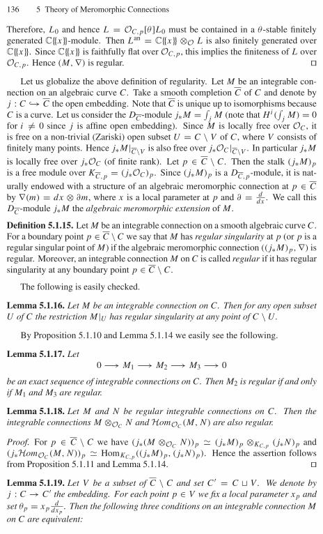
136 5 Theory of Meromorphic Connections
Therefore, L0 and hence L = OC,p[θ ]L0 must be contained in a θ -stable finitelygenerated C{{x}}-module. Then Lan = C{{x}} ⊗O L is also finitely generated overC{{x}}. Since C{{x}} is faithfully flat over OC,p, this implies the finiteness of L overOC,p. Hence (M, ∇) is regular. ��
Let us globalize the above definition of regularity. Let M be an integrable con-nection on an algebraic curve C. Take a smooth completion C of C and denote byj : C ↪→ C the open embedding. Note that C is unique up to isomorphisms becauseC is a curve. Let us consider the DC-module j∗M = ∫
jM (note that Hi(
∫j
M) = 0for i = 0 since j is affine open embedding). Since M is locally free over OC , itis free on a non-trivial (Zariski) open subset U = C \ V of C, where V consists offinitely many points. Hence j∗M|C\V is also free over j∗OC |C\V . In particular j∗M
is locally free over j∗OC (of finite rank). Let p ∈ C \ C. Then the stalk (j∗M)p
is a free module over KC,p = (j∗OC)p. Since (j∗M)p is a DC,p-module, it is nat-
urally endowed with a structure of an algebraic meromorphic connection at p ∈ C
by ∇(m) = dx ⊗ ∂m, where x is a local parameter at p and ∂ = ddx
. We call thisDC-module j∗M the algebraic meromorphic extension of M .
Definition 5.1.15. Let M be an integrable connection on a smooth algebraic curve C.For a boundary point p ∈ C \ C we say that M has regular singularity at p (or p is aregular singular point of M) if the algebraic meromorphic connection ((j∗M)p, ∇) isregular. Moreover, an integrable connection M on C is called regular if it has regularsingularity at any boundary point p ∈ C \ C.
The following is easily checked.
Lemma 5.1.16. Let M be an integrable connection on C. Then for any open subsetU of C the restriction M|U has regular singularity at any point of C \ U .
By Proposition 5.1.10 and Lemma 5.1.14 we easily see the following.
Lemma 5.1.17. Let0 −→ M1 −→ M2 −→ M3 −→ 0
be an exact sequence of integrable connections on C. Then M2 is regular if and onlyif M1 and M3 are regular.
Lemma 5.1.18. Let M and N be regular integrable connections on C. Then theintegrable connections M ⊗OC
N and HomOC(M, N) are also regular.
Proof. For p ∈ C \ C we have (j∗(M ⊗OCN))p � (j∗M)p ⊗KC,p
(j∗N)p and(j∗HomOC
(M, N))p � HomKC,p((j∗M)p, (j∗N)p). Hence the assertion follows
from Proposition 5.1.11 and Lemma 5.1.14. ��Lemma 5.1.19. Let V be a subset of C \ C and set C′ = C � V . We denote byj : C → C′ the embedding. For each point p ∈ V we fix a local parameter xp andset θp = xp
ddxp
. Then the following three conditions on an integrable connection M
on C are equivalent:
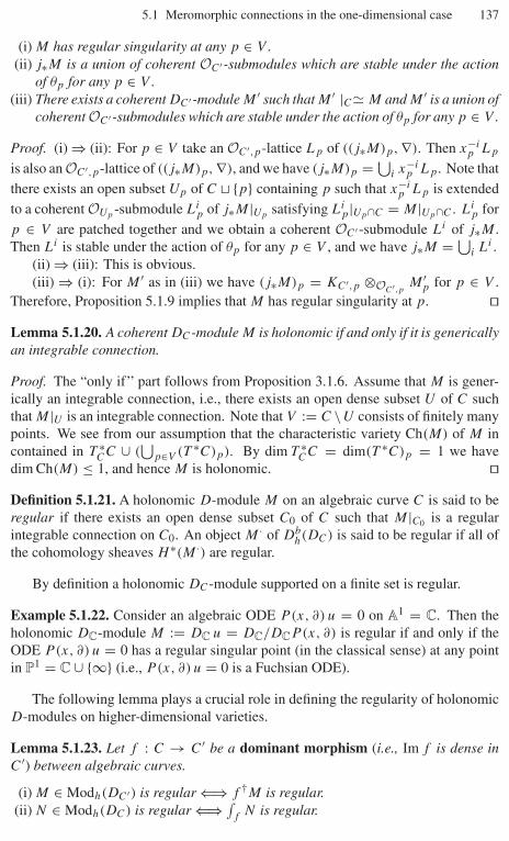
5.1 Meromorphic connections in the one-dimensional case 137
(i) M has regular singularity at any p ∈ V .(ii) j∗M is a union of coherent OC′ -submodules which are stable under the action
of θp for any p ∈ V .(iii) There exists a coherent DC′ -module M ′ such that M ′ |C� M and M ′ is a union of
coherent OC′ -submodules which are stable under the action of θp for any p ∈ V .
Proof. (i) ⇒ (ii): For p ∈ V take an OC′,p-lattice Lp of ((j∗M)p, ∇). Then x−ip Lp
is also an OC′,p-lattice of ((j∗M)p, ∇), and we have (j∗M)p = ⋃i x−i
p Lp. Note thatthere exists an open subset Up of C � {p} containing p such that x−i
p Lp is extendedto a coherent OUp -submodule Li
p of j∗M|Up satisfying Lip|Up∩C = M|Up∩C . Li
p forp ∈ V are patched together and we obtain a coherent OC′ -submodule Li of j∗M .Then Li is stable under the action of θp for any p ∈ V , and we have j∗M = ⋃
i Li .(ii) ⇒ (iii): This is obvious.(iii) ⇒ (i): For M ′ as in (iii) we have (j∗M)p = KC′,p ⊗OC′,p M ′
p for p ∈ V .Therefore, Proposition 5.1.9 implies that M has regular singularity at p. ��Lemma 5.1.20. A coherent DC-module M is holonomic if and only if it is genericallyan integrable connection.
Proof. The “only if’’ part follows from Proposition 3.1.6. Assume that M is gener-ically an integrable connection, i.e., there exists an open dense subset U of C suchthat M|U is an integrable connection. Note that V := C \U consists of finitely manypoints. We see from our assumption that the characteristic variety Ch(M) of M incontained in T ∗
CC ∪ (⋃
p∈V (T ∗C)p). By dim T ∗CC = dim(T ∗C)p = 1 we have
dim Ch(M) ≤ 1, and hence M is holonomic. ��Definition 5.1.21. A holonomic D-module M on an algebraic curve C is said to beregular if there exists an open dense subset C0 of C such that M|C0 is a regularintegrable connection on C0. An object M · of Db
h(DC) is said to be regular if all ofthe cohomology sheaves H ∗(M ·) are regular.
By definition a holonomic DC-module supported on a finite set is regular.
Example 5.1.22. Consider an algebraic ODE P(x, ∂) u = 0 on A1 = C. Then theholonomic DC-module M := DC u = DC/DCP(x, ∂) is regular if and only if theODE P(x, ∂) u = 0 has a regular singular point (in the classical sense) at any pointin P1 = C ∪ {∞} (i.e., P(x, ∂) u = 0 is a Fuchsian ODE).
The following lemma plays a crucial role in defining the regularity of holonomicD-modules on higher-dimensional varieties.
Lemma 5.1.23. Let f : C → C′ be a dominant morphism (i.e., Im f is dense inC′) between algebraic curves.
(i) M ∈ Modh(DC′) is regular ⇐⇒ f †M is regular.(ii) N ∈ Modh(DC) is regular ⇐⇒ ∫
fN is regular.
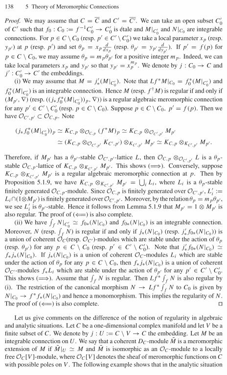
138 5 Theory of Meromorphic Connections
Proof. We may assume that C = C and C′ = C′. We can take an open subset C′0
of C′ such that f0 : C0 := f −1C′0 → C′
0 is étale and M|C′0
and N |C0 are integrableconnections. For p ∈ C \ C0 (resp. p′ ∈ C′ \ C′
0) we take a local parameter xp (resp.yp′ ) at p (resp. p′) and set θp = xp
ddxp
(resp. θp′ = yp′ ddyp′ ). If p′ = f (p) for
p ∈ C \ C0, we may assume θp = mpθp′ for a positive integer mp. Indeed, we cantake local parameters xp and yp′ so that yp′ = x
mpp . We denote by j : C0 → C and
j ′ : C′0 → C′ the embeddings.
(i) We may assume that M = j ′∗(M|C′0). Note that Lf ∗M|C0 = f ∗
0 (M|C′0) and
f ∗0 (M|C′
0) is an integrable connection. Hence M (resp. f †M) is regular if and only if
(Mp′ , ∇) (resp. ((j∗f ∗0 (M|C′
0))p, ∇)) is a regular algebraic meromorphic connection
for any p′ ∈ C′ \ C′0 (resp. p ∈ C \ C0). Suppose p ∈ C \ C0, p′ = f (p). Then we
have OC′,p′ ⊂ OC,p. Note
(j∗f ∗0 (M|C′
0))p � KC,p ⊗OC,p
(f ∗M)p � KC,p ⊗OC′,p′ Mp′
� (KC,p ⊗OC′,p′ KC′,p′) ⊗KC′,p′ Mp′ � KC,p ⊗KC′,p′ Mp′ .
Therefore, if Mp′ has a θp′ -stable OC′,p′ -lattice L, then OC,p ⊗OC′,p′ L is a θp-stable OC,p-lattice of KC,p ⊗KC′,p′ Mp′ . This shows (=⇒). Conversely, supposeKC,p ⊗KC′,p′ Mp′ is a regular algebraic meromorphic connection at p. Then byProposition 5.1.9, we have KC,p ⊗KC′,p′ Mp′ = ⋃
i Li , where Li is a θp-stablefinitely generated OC,p-module. Since OC,p is finitely generated over OC′,p′ , L′
i :=Li∩(1⊗Mp′) is finitely generated overOC′,p′ . Moreover, by the relation θp = mpθp′ ,we see L′
i is θp′ -stable. Hence it follows from Lemma 5.1.9 that Mp′ = 1 ⊗ Mp′ isalso regular. The proof of (⇐=) is also complete.
(ii) We have∫
fN |C′
0� f0∗(N |C0) and f0∗(N |C0) is an integrable connection.
Moreover, N (resp.∫
fN ) is regular if and only if j∗(N |C0) (resp. j ′∗f0∗(N |C0)) is
a union of coherent OC(resp. OC′ )-modules which are stable under the action of θp
(resp. θp′ ) for any p ∈ C \ C0 (resp. p′ ∈ C′ \ C′0). Note that j ′∗f0∗(N |C0) �
f∗j∗(N |C0). If j∗(N |C0) is a union of coherent OC-modules Li which are stableunder the action of θp for any p ∈ C \ C0, then f∗j∗(N |C0) is a union of coherentOC′ -modules f∗Li which are stable under the action of θp′ for any p′ ∈ C′ \ C′
0.This shows (=⇒). Assume that
∫f
N is regular. Then Lf ∗ ∫f
N is also regular by
(i). The restriction of the canonical morphism N → Lf ∗ ∫f
N to C0 is given byN |C0 → f ∗f∗(N |C0) and hence a monomorphism. This implies the regularity of N .The proof of (⇐=) is also complete. ��
Let us give comments on the difference of the notion of regularity in algebraicand analytic situations. Let C be a one-dimensional complex manifold and let V be afinite subset of C. We denote by j : U := C \ V → C the embedding. Let M be anintegrable connection on U . We say that a coherent DC-module M is a meromorphicextension of M if M|U � M and M is isomorphic as an OC-module to a locallyfree OC[V ]-module, where OC[V ] denotes the sheaf of meromorphic functions on C
with possible poles on V . The following example shows that in the analytic situation
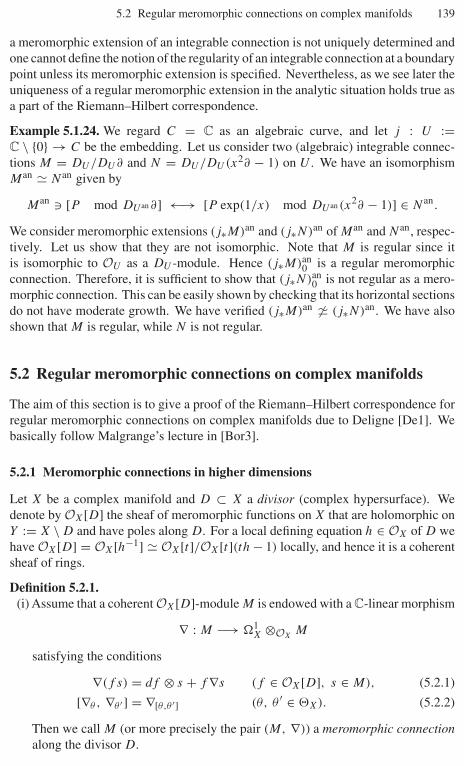
5.2 Regular meromorphic connections on complex manifolds 139
a meromorphic extension of an integrable connection is not uniquely determined andone cannot define the notion of the regularity of an integrable connection at a boundarypoint unless its meromorphic extension is specified. Nevertheless, as we see later theuniqueness of a regular meromorphic extension in the analytic situation holds true asa part of the Riemann–Hilbert correspondence.
Example 5.1.24. We regard C = C as an algebraic curve, and let j : U :=C \ {0} → C be the embedding. Let us consider two (algebraic) integrable connec-tions M = DU /DU ∂ and N = DU /DU (x2∂ − 1) on U . We have an isomorphismMan � Nan given by
Man [P mod DU an ∂] ←→ [P exp(1/x) mod DU an (x2∂ − 1)] ∈ Nan.
We consider meromorphic extensions (j∗M)an and (j∗N)an of Man and Nan, respec-tively. Let us show that they are not isomorphic. Note that M is regular since itis isomorphic to OU as a DU -module. Hence (j∗M)an
0 is a regular meromorphicconnection. Therefore, it is sufficient to show that (j∗N)an
0 is not regular as a mero-morphic connection. This can be easily shown by checking that its horizontal sectionsdo not have moderate growth. We have verified (j∗M)an � (j∗N)an. We have alsoshown that M is regular, while N is not regular.
5.2 Regular meromorphic connections on complex manifolds
The aim of this section is to give a proof of the Riemann–Hilbert correspondence forregular meromorphic connections on complex manifolds due to Deligne [De1]. Webasically follow Malgrange’s lecture in [Bor3].
5.2.1 Meromorphic connections in higher dimensions
Let X be a complex manifold and D ⊂ X a divisor (complex hypersurface). Wedenote by OX[D] the sheaf of meromorphic functions on X that are holomorphic onY := X \ D and have poles along D. For a local defining equation h ∈ OX of D wehave OX[D] = OX[h−1] � OX[t]/OX[t](th − 1) locally, and hence it is a coherentsheaf of rings.
Definition 5.2.1.(i) Assume that a coherent OX[D]-module M is endowed with a C-linear morphism
∇ : M −→ �1X ⊗OX
M
satisfying the conditions
∇(f s) = df ⊗ s + f ∇s (f ∈ OX[D], s ∈ M), (5.2.1)
[∇θ , ∇θ ′ ] = ∇[θ,θ ′] (θ, θ ′ ∈ �X). (5.2.2)
Then we call M (or more precisely the pair (M, ∇)) a meromorphic connectionalong the divisor D.
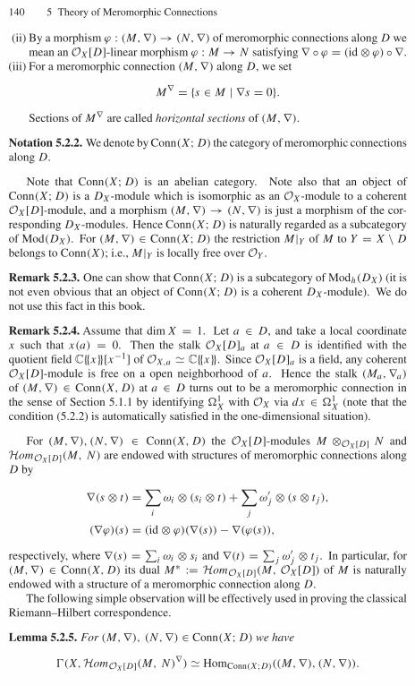
140 5 Theory of Meromorphic Connections
(ii) By a morphism ϕ : (M, ∇) → (N, ∇) of meromorphic connections along D wemean an OX[D]-linear morphism ϕ : M → N satisfying ∇ ◦ ϕ = (id ⊗ ϕ) ◦ ∇.
(iii) For a meromorphic connection (M, ∇) along D, we set
M∇ = {s ∈ M | ∇s = 0}.Sections of M∇ are called horizontal sections of (M, ∇).
Notation 5.2.2. We denote by Conn(X; D) the category of meromorphic connectionsalong D.
Note that Conn(X; D) is an abelian category. Note also that an object ofConn(X; D) is a DX-module which is isomorphic as an OX-module to a coherentOX[D]-module, and a morphism (M, ∇) → (N, ∇) is just a morphism of the cor-responding DX-modules. Hence Conn(X; D) is naturally regarded as a subcategoryof Mod(DX). For (M, ∇) ∈ Conn(X; D) the restriction M|Y of M to Y = X \ D
belongs to Conn(X); i.e., M|Y is locally free over OY .
Remark 5.2.3. One can show that Conn(X; D) is a subcategory of Modh(DX) (it isnot even obvious that an object of Conn(X; D) is a coherent DX-module). We donot use this fact in this book.
Remark 5.2.4. Assume that dim X = 1. Let a ∈ D, and take a local coordinatex such that x(a) = 0. Then the stalk OX[D]a at a ∈ D is identified with thequotient field C{{x}}[x−1] of OX,a � C{{x}}. Since OX[D]a is a field, any coherentOX[D]-module is free on a open neighborhood of a. Hence the stalk (Ma, ∇a)
of (M, ∇) ∈ Conn(X, D) at a ∈ D turns out to be a meromorphic connection inthe sense of Section 5.1.1 by identifying �1
X with OX via dx ∈ �1X (note that the
condition (5.2.2) is automatically satisfied in the one-dimensional situation).
For (M, ∇), (N, ∇) ∈ Conn(X, D) the OX[D]-modules M ⊗OX[D] N andHomOX[D](M, N) are endowed with structures of meromorphic connections alongD by
∇(s ⊗ t) =∑
i
ωi ⊗ (si ⊗ t) +∑
j
ω′j ⊗ (s ⊗ tj ),
(∇ϕ)(s) = (id ⊗ ϕ)(∇(s)) − ∇(ϕ(s)),
respectively, where ∇(s) = ∑i ωi ⊗ si and ∇(t) = ∑
j ω′j ⊗ tj . In particular, for
(M, ∇) ∈ Conn(X, D) its dual M∗ := HomOX[D](M, OX[D]) of M is naturallyendowed with a structure of a meromorphic connection along D.
The following simple observation will be effectively used in proving the classicalRiemann–Hilbert correspondence.
Lemma 5.2.5. For (M, ∇), (N, ∇) ∈ Conn(X; D) we have
�(X, HomOX[D](M, N)∇) � HomConn(X;D)((M, ∇), (N, ∇)).
5.2 Regular meromorphic connections on complex manifolds 141
Proposition 5.2.6. Let ϕ : M1 → M2 be a morphism of meromorphic connectionsalong D. If ϕ|X\D is an isomorphism, then ϕ is an isomorphism.
This follows from the following lemma since the kernel and the cokernel of ϕ arecoherent OX[D]-modules supported by D.
Lemma 5.2.7. A coherent OX[D]-module M whose support is contained in D istrivial; M = 0.
Proof. Take a local defining equation h of D. For a section s ∈ M whose support iscontained in D consider the OX-coherent submodule OXs ⊂ M . Since the supportof OXs is contained in D, we have hNs = 0 (N � 0) by Hilbert’s Nullstellensatz.Therefore, we obtain s = h−NhNs = 0. ��Corollary 5.2.8. Any meromorphic connection M along D is reflexive in the sensethat the canonical morphism M → M∗∗ is an isomorphism.
Let f : Z → X be a morphism of complex manifolds such that f −1D is a divisoron Z. Then we have
OZ[f −1D] � OZ ⊗f −1OXf −1OX[D] � OZ ⊗L
f −1OXf −1OX[D].
Indeed, since OX[D] is flat over OX, we have Hi(OZ ⊗Lf −1OX
f −1OX[D]) = 0for i = 0. Moreover, for a local defining equation h = 0 of D we haveOX[D] = OX[h−1], OZ[f −1D] = OZ[h◦f ] and hence OZ[f −1D] � OZ ⊗f −1OX
f −1OX[D]. Hence for M ∈ Conn(X; D) we have
Lf ∗M � OZ ⊗Lf −1OX
f −1M � OZ[f −1D] ⊗Lf −1OX[D] f −1M
� OZ[f −1D] ⊗f −1OX[D] f −1M.
From this we easily see the following.
Lemma 5.2.9. Let f be as above. For any M ∈ Conn(X; D) we have Hj (Lf ∗M) =0 for j = 0 and H 0(Lf ∗M) ∈ Conn(Z; f −1D). In particular, the inverse imagefunctor for the category of D-modules induces an exact functor
f ∗ : Conn(X; D) → Conn(Z; f −1D).
SetB = {x ∈ C | |x| < 1} (the unit disk).
For a morphism i : B → X such that i−1D = {0} the stalk (i∗M)0 at 0 ∈ B is ameromorphic connection of one-variable studied in Section 5.1.1.
Definition 5.2.10. A meromorphic connection M on X along D is called regular if(i∗M)0 is regular in the sense of Section 5.1.2 for any morphism i : B → X suchthat i−1D = {0} ⊂ B.
142 5 Theory of Meromorphic Connections
Notation 5.2.11. We denote by Connreg(X; D) the category of regular meromorphicconnections along D.
Proposition 5.2.12.(i) Let
0 → M1 → M2 → M3 → 0
be a short exact sequence of meromorphic connections along D. Then M2 isregular if and only if M1 and M3 are regular.
(ii) Assume that M and N are regular meromorphic connections along D. ThenM ⊗OX[D] N and HomOX[D](M, N) are also regular.
Proof. By definition we can reduce the problem to the case when X is the unit diskB ⊂ C. Then (i) follows from Proposition 5.1.10. We can prove (ii) by usingLemma 5.1.11. This completes the proof. ��Definition 5.2.13. A meromorphic connection on X along D is called effective if it isgenerated as an OX[D]-module by a coherent OX-submodule.
We will see later that any regular meromorphic connection is effective (see Corol-lary 5.2.22 (ii) below).
Lemma 5.2.14. Let f : X′ → X be a proper surjective morphism of complex man-ifolds such that D′ := f −1D is a divisor on X′ and f −1(X′ \ D′) → X \ D is anisomorphism. Assume that N is an effective meromorphic connection on X′ along D′.
(i) We have Hk(∫
fN) = 0 for k = 0 and H 0(
∫f
N) is an effective meromorphicconnection on X along D.
(ii) If N is regular, then so is H 0(∫
fN).
Proof. We denote by DX′ [D′] the subalgebra of EndC(OX′ [D′]) generated by DX′and OX′ [D′]. Then we have DX′ [D′] � DX′ ⊗OX′ OX′ [D′] � OX′ [D′] ⊗OX′ DX′ .
We first show that
DX←X′ ⊗LDX′ DX′ [D′] � DX′ [D′]. (5.2.3)
Note that the canonical morphism f −1�X → �X′ induces an isomorphismOX′ [D′] ⊗f −1OX
f −1�X → OX′ [D′] ⊗OX′ �X′ by Lemma 5.2.7. Hence we have
DX←X′ ⊗LDX′ DX′ [D′] � DX←X′ ⊗L
OX′ OX′ [D′]� DX←X′ ⊗OX′ OX′ [D′]� f −1DX ⊗f −1OX
OX′ [D′]by Lemma 1.3.4. Let us show that the canonical morphism DX′ [D′] →f −1DX ⊗f −1OX
OX′ [D′] induced by the canonical section 1⊗1 of the right DX′ [D′]-module f −1DX ⊗f −1OX
OX′ [D′] is an isomorphism. For this it is sufficient to show
5.2 Regular meromorphic connections on complex manifolds 143
that FpDX′ [D′] → f −1FpDX ⊗f −1OXOX′ [D′] is an isomorphism for any p ∈ Z.
This follows from Lemma 5.2.7. The assertion (5.2.3) is verified.Since N is effective, there exists a coherent OX′ -submodule L of N such that
N � OX′ [D′] ⊗OX′ L. Then by (5.2.3) and f −1OX[D] ⊗f −1OXOX′ � OX′ [D′],
we have∫f
N = Rf∗(DX←X′ ⊗LDX′ N) � Rf∗(DX←X′ ⊗L
DX′ DX′ [D′] ⊗LDX′ [D′] N)
� Rf∗(N) � Rf∗(OX′ [D′] ⊗OX′ L) � Rf∗(f −1OX[D] ⊗f −1OXL)
� OX[D] ⊗OXRf∗(L),
and hence Hk(∫
fN) � OX[D] ⊗OX
Hk(Rf∗(L)). Since Hk(Rf∗(L)) is coherent
over OX for any k by the Grauert direct image theorem, Hk(∫
fN) is coherent over
OX[D]. Moreover, we have Hk(∫
fN) = 0 for k = 0 by Hk(Rf∗(L))|X\D = 0 and
Lemma 5.2.7. The statement (i) is proved.Assume that N is regular. Let i : B → X be a morphism from the unit disk B
satisfying i−1(D) = {0}. Since f is proper, there exists a lift j : B → X′ satisfyingf ◦ j = i. Then we have
i∗H 0(∫
f
N)
� i∗∫
f
N � j∗f ∗∫
f
N.
Since the canonical morphism N → f ∗ ∫f
N is an isomorphism on X′ \ D′, it is
an isomorphism on X′ by Proposition 5.2.6. Hence we obtain i∗H 0(∫
fN) � j∗N .
Therefore, H 0(∫
fN) is regular. The statement (ii) is proved. ��
5.2.2 Meromorphic connections with logarithmic poles
In this subsection we will consider the case where D is a normal crossing divisor ona complex manifold X; i.e., we assume that D is locally defined by a function of theform x1 · · · xr , where (x1, . . . , xn) is a local coordinate. Let p ∈ D and fix such acoordinate (x1, . . . , xn) around p ∈ D. For 1 ≤ k ≤ r we denote by Dk the (local)irreducible component of D defined by xk .
The meromorphic connections M on X along D which we will consider in thissubsection are also of very special type. First, we assume that there exists a holo-morphic vector bundle (locally free OX-module of finite rank) L on X such thatM = OX[D] ⊗OX
L as an OX[D]-module. Hence taking a local defining equationx1x2 · · · xr = 0 of D and choosing a basis e1, e2, . . . , em of L around a point p ∈ D,the associated C-linear morphism ∇ : M → �1
X ⊗OXM can be expressed as
∇ei =∑
1≤k≤n,1≤j≤m
akij dxk ⊗ ej , (5.2.4)
where akij ∈ OX[D] = OX[x−1
1 x−12 · · · x−1
r ]. Then we further assume that the
functions xkakij (1 ≤ k ≤ r), ak
ij (r < k ≤ n) are holomorphic. In this case, we say

144 5 Theory of Meromorphic Connections
the meromorphic connection M along the normal crossing divisor D has a logarithmicpole with respect to the lattice L at p. If this is the case at any p ∈ D, we say that M
has a logarithmic pole along D with respect to L. Note that this definition does notdepend on the choice of the coordinates {xk} and the basis {ei} of L.
Let M be a meromorphic connection along D which has a logarithmic pole withrespect to the lattice L. Take a basis {e1, . . . , em} of L and set Ak = (ak
ij ) for 1 ≤ k ≤n, where ak
ij is as in (5.2.4). For 1 ≤ k ≤ r we also set Bk = xkAk . Let 1 ≤ k ≤ r .Since Bk belongs to Mm(OX), we can consider its restriction Bk|Dk
∈ Mm(ODk).
Then Bk|Dkdefines a canonical section ResL
Dk∇ of the vector bundle EndODk
(L|Dk)
on Dk . Indeed, we can check easily that Bk|Dk∈ Mm(ODk
) � EndODk(L|Dk
) does
not depend on the choice of a local coordinate and a basis of L. We call ResLDk
∇ theresidue of (M, ∇) along Dk .
Proposition 5.2.15. Let M be a meromorphic connection along D which has a log-arithmic pole with respect to the lattice L. We keep the notation as above.
(i) On Dk ∩ Dl we have[ResL
Dk∇, ResL
Dl∇] = 0.
(ii) The eigenvalues of (ResLDk
∇)(a) ∈ EndC(L(a)) do not depend on the choice ofa ∈ Dk . Here L(a) denotes the fiber C ⊗OX,a
La of L at a.
Proof. (i) By (5.2.2) we have
∂Ak
∂xl
− ∂Al
∂xk
= [Ak, Al].
We obtain the desired result from this by developing both sides into the Laurent serieswith respect to xk, xl and comparing the coefficients of (xkxl)
−1.
(ii) Let Ap, B
kbe the restrictions of the matrices Ap, Bk to Dk , respectively.
Then we have
∂Ai
∂xj
− ∂Aj
∂xi
= [Ai, A
j ] (i, j = k),
∂Bk
∂xi
= [Bk, A
i] (i = k).
The first formula implies that
∇ei =∑l =k
alij dxl ⊗ ej (A
l = (alij ))
defines an integrable connection ∇ on L|Dk. The second one implies that B
k =ResL
Dk∇ ∈ EndODk
L|Dkis a horizontal section with respect to the connection induced
by ∇ on EndODkL|Dk
. From this we can easily check that the values of the matrix
Bk
at two different points of Dk are conjugate to each other. ��
5.2 Regular meromorphic connections on complex manifolds 145
Proposition 5.2.16. Let M be a meromorphic connection which has a logarithmicpole along D with respect to a lattice L. Then M is regular.
Proof. For any morphism i : B → X from the unit disk B such that i−1D = {0} weeasily see that the meromorphic connection i∗M on B has a logarithmic pole along{0} with respect to the lattice i∗L. Then the stalk (i∗M)0 is regular by Theorem 5.1.4.
��The following construction enables us to extend analytic integrable connections
on Y = X \ D to regular meromorphic connections along the divisor D ⊂ X.
Theorem 5.2.17. Let D be a normal crossing divisor on X and set Y := X \ D. Wefix a section τ : C/Z ↪→ C of the projection C → C/Z. Then for an integrableconnection M on Y there exists an extension Lτ of M as a vector bundle on X
satisfying the following two conditions:
(i) The C-linear morphism ∇M : M → �1Y ⊗OY
M can be uniquely extended to aC-linear morphism ∇ : OX[D] ⊗OX
Lτ → �1X ⊗OX
(OX[D] ⊗OXLτ ) so that
(OX[D]⊗OXLτ , ∇) is a meromorphic connection which has a logarithmic pole
along D with respect to Lτ .(ii) For any irreducible component D′ of D the eigenvalues of the residue ResLτ
D′ ∇of (OX[D] ⊗OX
Lτ , ∇) along D′ are contained in τ(C/Z) ⊂ C.
Moreover, such an extension is unique up to isomorphisms.
Proof. First we prove the uniqueness of the extension. The problem being local, wemay assume X = Bn (B is a unit disk in C) and Y = (B∗)r × Bn−r (B∗ := B \ {0}).We denote by {xi}1≤i≤n the standard coordinate of X = Bn Let L, L′ be locally freeOX-modules of rank m satisfying the conditions (i), (ii) for Lτ = L and Lτ = L′,and let ∇ : OX[D] ⊗OX
L → �1X ⊗OX
OX[D] ⊗OXL and ∇′ : OX[D] ⊗OX
L′ →�1
X ⊗OXOX[D]⊗OX
L′ be the C-linear morphisms satisfying the condition (i). Takea basis {ei}1≤i≤m of L. Then ∇ can be expressed as
∇ei =∑k,j
akij dxk ⊗ ej .
Set ω = ∑1≤k≤n Akdxk (Ak = (ak
ij )). We also fix a basis {e′i} of L′ and define
ω′ = ∑1≤k≤n A′kdxk similar to ω. Since L|Y and L′|Y are isomorphic, there exists
S ∈ GLm(OY ) such thatdS = Sω − ω′S. (5.2.5)
It is sufficient to verify that S and S−1 can be extended to an element of Mm(OX)
(an m×m matrix on X whose entries are holomorphic on X). By symmetry we haveonly to show the assertion for S. Moreover, by Hartogs’ theorem it is sufficient toshow that S extends holomorphically across Dk \⋃l =k Dl for each k. For simplicityof notation we only consider the case k = 1. Write
146 5 Theory of Meromorphic Connections
ω = B1 dx1
x1+∑i>1
Aidxi,
ω′ = B ′1 dx1
x1+∑i>1
A′idxi .
By our assumption B1, B ′1 and Ai , A′i are holomorphic on x2x3 · · · xr = 0. By(5.2.5) we have
x1∂S
∂x1= SB1 − B ′1S. (5.2.6)
Taking the matrix norm ‖•‖ of both sides we obtain an inequality
|x1|∥∥∥∥ ∂S
∂x1
∥∥∥∥ ≤ C ‖S‖ (5.2.7)
(C > 0 is a constant) on a neighborhood of x1 = 0 (x2x3 · · · xr = 0), from whichwe see that S is meromorphic along D1 \ ⋃i =1 Di by Gronwall’s inequality: iff (t) ≥ 0, g(t) ≥ 0 are non-negative functions on 0 < t ≤ t0 such that
f (t) ≤ a + c
∫ t0
t
g(s)f (s)ds (a ≥ 0, c ≥ 0),
then we have
f (t) ≤ a exp(c
∫ t0
t
g(s)ds) (0 < t < t0).
To show that S is actually holomorphic on D1 \⋃i =1 Di we consider the Laurentexpansion
S =∞∑
j=p
Sj xj
1 (Sp = 0)
of S with respect to the variable x1. By (5.2.6) we have
(ResD1 ∇′ + pI)Sp = Sp(ResD1 ∇),
where I is the unit matrix. By elementary linear algebra, it follows from Sp = 0 thatthe matrices ResD1 ∇′ +pI and ResD1 ∇ must have at least one common eigenvalue.If p = 0, then this last result contradicts our assumption that the eigenvalues ofResD1 ∇ and ResD1 ∇′ are contained in τ(C/Z). Hence we must have p = 0, and S
is holomorphic on D1 \⋃i =1 Di . The proof of the uniqueness is complete.Next we prove the existence of the extension (as a vector bundle) Lτ of M .
If there exists locally such an extension Lτ , we can glue these local extensions toget the global one by the uniqueness of Lτ proved above. Hence we may assumeY = (B∗)r × Bn−r ⊂ X = Bn. By Theorem 4.2.4 the integrable connection M onY is uniquely determined by the monodromy representation
ρ : π1(Y ) −→ GLm(C)

5.2 Regular meromorphic connections on complex manifolds 147
defined by the local system corresponding to M . Note that for Y = (B∗)r × Bn−r
we have π1(Y ) � Zr , where the element γi = (0, 0, . . . ,
i"
1 , . . . , 0) ∈ π1(Y ) � Zr
corresponds to a closed loop turning around the divisor Di = {xi = 0}. Therefore,the monodromy representation ρ is determined by the mutually commuting matrices
Ci := ρ(γi) ∈ GLm(C) (1 ≤ i ≤ r).
Note also that we can take matrices �i ∈ Mm(C) (1 ≤ i ≤ r) such that⎧⎪⎨⎪⎩(a) exp(2π
√−1 �i) = Ci,
(b) All the eigenvalues of �i belong to the set τ(C/Z),
(c) �i (1 ≤ i ≤ r) are mutually commuting matrices.
The proof of the existence of such matrices is left to the reader (in fact, �i areuniquely determined). Using these �i = (�i
pq) ∈ Mm(C), we define a meromorphicconnection on OX[D]m = OX[D] ⊗OX
Lτ (Lτ = OmX) by
∇eq = −∑
1≤i≤n,1≤q≤m
�ipq
xi
dxi ⊗ eq,
where {e1, . . . , em} is the standard basis of Lτ = OmX . Then the restriction of this
meromorphic connection to Y is isomorphic to M . Moreover, this meromorphicconnection satisfies all of the required conditions. ��
5.2.3 Deligne’s Riemann–Hilbert correspondence
In Theorem 5.2.17 we proved that an integrable connection M defined on the com-plementary set Y = X \ D of a normal crossing divisor D on X can be extended toa meromorphic connection M (= OX[D] ⊗OX
Lτ ) on X, regular along D. In thissubsection we generalize this result to arbitrary divisors D on X.
Let D be a (not necessarily normal crossing) divisor on X and (N, ∇) a mero-morphic connection on X which is meromorphic along D. We consider the followingcondition (R) on (N, ∇), which is a priori weaker than the regularity along D (in fact,we will prove in Corollary 5.2.22 below that these two conditions are equivalent).
Condition (R). There exists an open subset U of the regular part Dreg of D whichintersects with each connected component of Dreg and satisfies the condition:⎧⎪⎪⎨⎪⎪⎩
There exist an open neighborhood U of U in X and an isomorphismϕ : B × U
∼→ U such that ϕ|{0}×U = IdU and for each x ∈ U thepull-back (ϕ∗
xN, ϕ∗x∇) with respcet to ϕx = ϕ|B×{x} : B × {x} ↪→ X is
regular along {0} × {x}.Here B is the unit disk centered at 0 in C.
148 5 Theory of Meromorphic Connections
It is clear that if (N, ∇) is regular along D, then it satisfies the condition (R).
Lemma 5.2.18. Assume that a meromorphic connection (N, ∇) satisfies the condi-tion (R). Then the restriction map
�(X, N∇) −→ �(Y, N∇)
is an isomorphism.
Proof. The injectivity follows from Lemma 5.2.7. Let us show surjectivity. Weneed to show that any s ∈ �(Y, N∇) can be extended to a section of N∇ on X.By Corollary 5.2.8 it is sufficient to show that for any p ∈ D and any u ∈ N∗
p =HomOX[D](N, OX[D])p the function g = 〈u, s〉 is meromorphic at p. By Hartogs’theorem it is sufficient to show it in the case p ∈ Dreg.
We first deal with the case when p ∈ U ⊂ Dreg. Here U is as in Condition (R).We take a local coordinate (x1, . . . , xn) around p such that D is defined by x1 = 0and p corresponds to 0. We may assume that U = {0} × Bn−1. Let
g(x) =∑k∈Z
gk(x2, x3, . . . , xn) xk1
be the Laurent expansion of g with respect to x1. The condition (R) implies that foreach x′ = (x2, x3, . . . , xn) ∈ Bn−1 the restriction g|B∗×{x′} is meromorphic at thepoint {0} × {x′}. This means that for each x′ = (x2, x3, . . . , xn) ∈ Bn−1 we havegk(x′) = 0 (k # 0). For k ∈ Z set
Uk := { x′ = (x2, x3, . . . , xn) ∈ Bn−1 | gi(x′) = 0 (i ≤ k) }.
Then we have Bn−1 = ⋃k∈Z Uk and each Uk is a closed analytic subset of Bn−1. It
follows that we have Uk = Bn−1 for some k and hence g is meromorphic at p.Let us consider the general case p ∈ Dreg. We denote by K the subset of Dreg
consisting of p ∈ Dreg such that g = 〈u, s〉 is meromorphic at p for any u ∈ N∗p .
We need to show K = Dreg. Note that K is an open subset of Dreg containing U . Inparticular, it intersects with any connected component of Dreg. Hence it is sufficientto show that K is a closed subset of Dreg. Let q ∈ K . We take a local coordinate(x1, . . . , xn) around a such that D is defined by x1 = 0 and q corresponds to 0. Foru ∈ N∗
p we consider the expansion
g(x) =∑k∈Z
gk(x2, x3, . . . , xn) xk1
of g = 〈u, s〉. Since g is meromorphic on K , there exists some r such that gk = 0on K for any k ≤ r . It follows that gk = 0 for any k ≤ r on an open neighborhoodof q. Hence q ∈ K . ��Lemma 5.2.19. Let (Ni, ∇i ) (i = 1, 2) be two meromorphic connections along D
satisfying the condition (R). Then the restriction to Y = X\D induces an isomorphism
r : HomConn(X;D)((N1, ∇1), (N2, ∇2))∼→ HomConn(Y )((N1|Y , ∇1), (N2|Y , ∇2)).
5.2 Regular meromorphic connections on complex manifolds 149
Proof. By Lemma 5.2.5 we have
�(X, HomOX[D](N1, N2)∇) � HomConn(X;D)((N1, ∇1), (N2, ∇2)).
Therefore, it suffices to apply Lemma 5.2.18 to the meromorphic connection N =HomOX[D](N1, N2), which satisfies the condition (R) by Proposition 5.2.12 (ii). ��
The main result of this section is the following.
Theorem 5.2.20 (Deligne [De1]). Let X be a complex manifold and let D be a (notnecessarily normal crossing) divisor on X. Set Y = X \ D. Then the restrictionfunctor N �−→ N |Y induces an equivalence
Connreg(X; D) −→∼ Conn(Y )
of categories.
Proof. Since a regular meromorphic connection along D satisfies the condition (R),the restriction functor is fully faithful by Lemma 5.2.19. Let us prove the essentialsurjectivity. We take an integrable connection M on Y and consider the problem ofextending M to a regular meromorphic connection on the whole X. By Hironaka’stheorem there exists a proper surjective morphism f : X′ → X of complex manifoldssuch that D′ := f −1D is a normal crossing divisor on X′ and the restriction g :X′ \ D′ → X \ D = Y of f is an isomorphism. By Theorem 5.2.17 we can extendthe integrable connection g∗M on X′ \ D′ to a meromorphic connection N on X′along D′ which has a logarithmic pole with respect to a lattice L. Then H 0(
∫f
N)
satisfies the desired property by Lemma 5.2.14. ��When D is normal crossing, we proved in Theorem 5.2.17 the uniqueness of the
regular meromorphic extension of an integrable connection on Y under an additionalcondition about the lattice Lτ . Theorem 5.2.20 above asserts that this condition wasnot really necessary.
By Theorem 4.2.4 this theorem has the following topological interpretation.
Corollary 5.2.21. Let X be a complex manifold and let D be a divisor on X. SetY = X \ D. Then we have an equivalence
Connreg(X; D) −→∼ Loc(X \ D)
of categories.
We call this result Deligne’s Riemann–Hilbert correspondence. This classicalRiemann–Hilbert correspondence became the prototype of the Riemann–Hilbert cor-respondence for analytic regular holonomic D-modules (Theorem 7.2.1 below).
Corollary 5.2.22. Let D be a (not necessarily normal crossing) divisor on a complexmanifold X and let N be a meromorphic connection along D.
150 5 Theory of Meromorphic Connections
(i) If N satisfies the condition (R), then N is regular along D.(ii) If N is regular along D, then N is an effective meromorphic connection along D.
Proof. (i) By Theorem 5.2.20 there exists a regular meromorphic connection N1
along D such that N1|Y ∼→ N |Y . Since both N and N1 satisfy the condition (R),this isomorphism N1|Y ∼→ N |Y can be extended to a morphism N1 → N of mero-morphic connections on X by Lemma 5.2.19 . This is in fact an isomorphism byProposition 5.2.6, and hence N is regular along D.
(ii) In the proof of Theorem 5.2.20 we explicitly constructed a regular meromor-phic extension of N |Y , which is isomorphic to N and has the required property. ��
Assume that D is a normal crossing divisor on X. We define a subsheaf of thesheaf �X of holomorphic vector fields on X by
�X〈D〉 := { θ ∈ �X | θI ⊂ I },where I is the defining ideal of D. If {xi, ∂i} is a local coordinate system of X inwhich D is defined by x1x2 · · · xr = 0, then �X〈D〉 is generated by xi∂i (1 ≤ i ≤ r)
and ∂j (j > r) over OX.
Corollary 5.2.23. Assume that D is a normal crossing divisor on a complex manifoldX. Under the above notation the following conditions on a meromorphic connectionN along D are equivalent:
(i) N is regular along D.(ii) N is a union of �X〈D〉-stable coherent OX-submodules.
Proof. (i) =⇒ (ii): We use Theorem 5.2.17. Namely, for a section τ : C/Z ↪→ Cof C → C/Z, we take a locally free OX-module Lτ such that N |Y � Lτ |Yand OX[D] ⊗OX
Lτ is a regular meromorphic connection along D. Then byTheorem 5.2.20 we have N � OX[D] ⊗OX
Lτ . Taking a local coordinate sys-tem {xi} of X such that D is defined by g(x) = x1x2 · · · xr = 0, we haveOX[D] ⊗OX
Lτ = ⋃k≥0 OXg−k ⊗OX
Lτ . Since for each k ≥ 0 the definitionof the OX-coherent subsheaf OXg−k ⊗OX
Lτ of OX[D]⊗OXLτ does not depend on
the local coordinates {xi} or on the defining equation g of D, it is globally defined onthe whole X. Clearly each OXg−k ⊗OX
Lτ is �X〈D〉-stable (Lτ is �X〈D〉-stable).(ii) =⇒ (i): By Theorem 5.2.22 (i) it suffices to check that N satisfies the con-
dition (R). If we restrict N to a unit disk B in the condition (R), then the restrictedmeromorphic connection satisfies the condition (ii) on the unit disk B. By Propo-sition 5.1.9 this means that the restriction is a regular meromorphic connection at0 ∈ B. So N satisfies the condition (R). Now the proof is complete. ��Theorem 5.2.24 (Deligne [De1]). Let D be a divisor on a complex manifold X andlet j : Y = X \ D ↪→ X be the embedding. Let N be a regular meromorphicconnection along D. Then the natural morphisms{
DRX(N) −→ Rj∗j−1 DRX(N),
R�(X, DRX(N)) −→ R�(Y, DRY (N |Y ))
5.2 Regular meromorphic connections on complex manifolds 151
are isomorphisms.
Proof. It is enough to prove that DRX(N) → Rj∗j−1 DRX(N) is an isomorphism.We first show it in the case where D is normal crossing. The problem being
local on X, we may assume X = Bn and Y = (B∗)r × Bn−r , where B is the unitdisk in C and B∗ = B \ {0}. Recall that the category of meromorphic connectionsthat are regular along D is equivalent to that of local systems on Y . Hence byπ1((B∗)r × Bn−r ) � π(((C×)r × Cn−r )an) we can assume that X = (Cn)an andY = ((C×)r × Cn−r )an. Here, Cn, C×, Cn−r are regarded as algebraic varieties.We can assume also that N is a simple object in the abelian category of regularmeromorphic connections (along D). Indeed, let
0 −→ N1 −→ N2 −→ N3 −→ 0
be an exact sequence in this category, and denote by �i : DRX(Ni) −→Rj∗j−1 DRX(Ni) (i = 1, 2, 3) the natural morphisms. Then �2 is an isomorphismif �1 and �3 are as well. By
π1(Y ) = π1((C×)an)r × π1((Cn−r )an),
π1((C×)an) � Z, π1((Cn−r )an) = {1},we see that there exist λ1, . . . , λr ∈ C such that
N � (Nλ1 � · · · � Nλr � OCn−r )an. (5.2.8)
Here, for λ ∈ C we denote by Nλ the (algebraic) DC-module given by Nλ =DC/DC(x∂ − λ). Hence by Proposition 4.7.8 we obtain
DRX(N) � DRC(Nλ1) �C · · · �C DRC(Nλ1) �C C(Cn−r )an .
Therefore, it is sufficient to show DRC(Nλ) � Rk∗k−1 DRC(Nλ), where k : C× →C denotes the embedding (see Proposition 4.5.9). Since the canonical morphismDRC(Nλ) → Rk∗k−1 DRC(Nλ) is an isomorphism outside of the origin, we haveonly to show the isomorphism DRC(Nλ)0 � (Rk∗k−1 DRC(Nλ))0 for the stalks. Set∇ = ∂ + λ
x. Then (DRC(Nλ))0 (resp. (Rk∗k−1 DRC(Nλ))0) is represented by the
complex
[K ∇−→ K],(
resp. [K ∇−→ K])
,
where K = OCan [x−1] (resp. K = k∗O(C×)an ). From this we easily see by consid-ering the Laurent series expansions of functions in K and K that (DRC(Nλ))0 →(Rk∗k−1 DRC(Nλ))0 is an isomorphism.
Now we consider the general case where D is an arbitrary divisor on X. ByHironaka’s theorem there exists a proper surjective morphism f : X′ → X ofcomplex manifolds such that D′ := f −1D is a normal crossing divisor on X′ andthe restriction X′ \ D′ → X \ D = Y of f is an isomorphism. We denote byj ′ : X′ \ D′ → X′ the embedding. By Theorem 5.2.20 and Lemma 5.2.14 there
152 5 Theory of Meromorphic Connections
exists a regular meromorphic connection N ′ on X′ along D′ such that N � ∫f
N ′.Then we have
DRX(N) � DRX
(∫f
N ′) � Rf∗DRX′(N ′) � Rf∗Rj ′∗j ′−1DRX′(N ′)
� Rj∗j−1DRX(N)
by Theorem 4.2.5. The proof is complete. ��Remark 5.2.25. In the course of the proof of Theorem 5.2.24 we have used Propo-sition 4.7.8 and Proposition 4.5.9 in order to reduce the proof of the case of normalcrossing divisors to the one-dimensional situation. We can avoid this argument bydirectly considering DRX(N) as follows.
Let D be the normal crossing divisor on the complex manifold X = Cn defined byx1 · · · xr = 0, where (x1, . . . , xn) is the coordinate of Cn. Let N be the simple regularmeromorphic connection corresponding to the simple local system Cx
λ11 x
λ22 · · · xλr
r
(0 ≤ Re λi < 1) on Y = X \ D. Then N is identified with OX[D] as an OX[D]-module, and the action of ∂
∂xi(1 ≤ i ≤ n) is given by⎧⎪⎨⎪⎩
∇ ∂∂xi
u = ∂u
∂xi
− λi
xi
u, i = 1, 2, . . . , r
∇ ∂∂xi
u = ∂u
∂xi
, i = r + 1, r + 2, . . . , n
for u ∈ OX[D] (0 ≤ Re λi < 1). In this situation DRX(N) is represented bythe Koszul complex K(∇1, ∇2, . . . , ∇n; OX[D]) (up to some degree shift) definedby the mutually commuting differentials ∇i = ∇ d
dxi
: OX[D] −→ OX[D] (i =1, 2, . . . , n). On the other hands, Rj∗j−1 DRX(N) is represented by the Koszulcomplex K(∇1, ∇2, . . . , ∇n; j∗OX\D) because the hypersurface complement Y =X \ D is locally a Stein open subset of X = Cn. Hence it suffices to show that thenatural morphism
K(∇1, ∇2, . . . , ∇n; OX[D]) −→ K(∇1, ∇2, . . . , ∇n; j∗OX\D)
induced by OX[D] −→ j∗OX\D is a quasi-isomorphism. The sections of OX[D]have poles along D, while those of j∗OX\D may have essential singularities along D.We have to compare the cohomology groups of the de Rham complexes in these twodifferent sheaves. First, note that the Koszul complex K(∇1, ∇2, . . . , ∇n; OX[D])(resp. K(∇1, ∇2, . . . , ∇n; j∗OX\D)) is the simplified complex of the double complex
K(∇2, . . . , ∇n; OX[D] ∇1−→ OX[D]) (resp. K(∇2, . . . , ∇n; j∗OX\D∇1−→ j∗OX\D)
). Let us consider the morphism of complexes[OX[D] ∇1−→ OX[D]] −→ [
j∗OX\D∇1−→ j∗OX\D
]induced by OX[D] −→ j∗OX\D . We set X′ = {x1 = 0} ⊂ X and D′ = {x2 · · · xr =0} ⊂ X′. Then we can easily see that the cohomology groups of the left complex

5.3 Regular integrable connections on algebraic varieties 153
(resp. right complex) are OX′ [D′] (resp. j ′OX′\D′ , j ′ : X′ \ D′ ↪→ X′) or zero(it depends on the condition λ1 = 0 or not) by expanding the functions in OX[D](resp. in j∗OX\D) into the Laurent series in x1. So repeating this argument also forx2, x3, . . . , xn we can finally obtain the quasi-isomorphism
K(∇1, ∇2, . . . , ∇n; OX[D]) −→∼ K(∇1, ∇2, . . . , ∇n; j∗OX\D).
5.3 Regular integrable connections on algebraic varieties
In this subsection X denotes a smooth algebraic variety. The corresponding complexmanifold is denoted by Xan.
Assume that we are given an open embedding j : X ↪→ V of X into a smoothvariety V such that D := V \X is a divisor on V . We set OV [D] := j∗OX. As in theanalytic situation OV [D] is a coherent sheaf of rings. We say that a DV -module isan algebraic meromorphic connection along D if it is isomorphic as an OV -moduleto a coherent OV [D]-module. We denote by Conn(V ; D) the category of algebraicmeromorphic connections along D. It is an abelian category. Unlike the analyticsituation an extension of an integrable connection on X to an algebraic meromorphicconnection on V is unique as follows.
Lemma 5.3.1. The functor j−1 : Conn(V ; D) → Conn(X) induces an equivalence
Conn(V ; D) −→∼ Conn(X)
of categories. Its quasi-inverse is given by j∗.
Proof. This follows easily from the fact that the category of coherent OV [D]-modulesis naturally equivalent to that of coherent OX-modules. ��
It follows that Conn(V ; D) is a subcategory of Modh(DV ) by Theorem 3.2.3 (i).
Definition 5.3.2. An integrable connection M on X is called regular if for any mor-phism iC : C → X from a smooth algebraic curve C the induced integrable connec-tion i∗CM on C is regular in the sense of Section 5.1.3.
Notation 5.3.3. We denote by Connreg(X) the full subcategory Conn(X) consistingof regular integrable connections.
By Lemma 5.1.17 we have the following.
Proposition 5.3.4. Let
0 −→ M1 −→ M2 −→ M3 −→ 0
be an exact sequence of integrable connections on X. Then M2 is regular if and onlyif M1 and M3 are regular.
154 5 Theory of Meromorphic Connections
By Lemma 5.1.18 we easily see the following.
Proposition 5.3.5. Let M and N be regular integrable connections on X. Then theintegrable connections M ⊗OX
N and HomOX(M, N) are also regular.
We give below some criteria for the regularity of integrable connections. Let ustake a smooth completion j : X ↪→ X of X such that D = X \ X is a divisor onX. Such a completion always exists thanks to Hironaka’s theorem (in fact, we cantake a completion X so that D = X \ X is a normal crossing divisor). We call sucha completion X of X a divisor completion. For a divisor completion j : X ↪→ X ofX we can consider the analytic meromorphic connection
(j∗M)an = OX
an ⊗OXj∗M ∈ Conn(X
an; Dan)
on Xan
along Dan.
Proposition 5.3.6. The following three conditions on an integrable connection M onX are equivalent:
(i) M is a regular integrable connection.(ii) For some divisor completion j : X ↪→ X of X the analytic meromorphic con-
nection (j∗M)an is regular.(iii) For any divisor completion j : X ↪→ X of X the analytic meromorphic connec-
tion (j∗M)an is regular.
Proof. We first prove the part (ii) =⇒ (i). Assume that for a divisor completionj : X ↪→ X the meromorphic connection (j∗M)an is regular. We need to show thatfor any morphism iC : C → X from an algebraic curve C the induced integrableconnection i∗CM is regular. We may assume that the image of C is not a single point.We take a smooth completion jC : C ↪→ C of C and a morphism iC : C → X sothat the following diagram:
CjC−−−−→ C
iC
⏐⏐ iC
⏐⏐X
j−−−−→ X
is commutative. We may also assume that this diagram is cartesian by replacing C
with (iC)−1(X) (see Lemma 5.1.16). In this situation we have a natural isomorphism[(jC)∗i∗CM
]an � [i∗C
j∗M]an � (ian
C)∗(j∗M)an.
Since (j∗M)an is regular, (ianC
)∗(j∗M)an (and hence[(jC)∗i∗CM
]an) is regular by thedefinition of (analytic) regular meromorphic connections. It follows that i∗CM isregular by Lemma 5.1.14. It remains to show (i) =⇒ (iii). By Corollary 5.2.22 (i) itis sufficient to verify the condition (R) for (j∗M)an. We can take ϕ in the condition(R) so that ϕx = ϕ|B×{x} comes from an algebraic morphism, for which the condition(R) can be easily checked by the argument used in the proof of (ii) =⇒ (i). ��
5.3 Regular integrable connections on algebraic varieties 155
Let j : X ↪→ X be a divisor completion of X such that D = X \ X is normalcrossing. In this situation we give another criterion of the regularity of an integrableconnection M on X. Let I be the defining ideal of D (I := {ϕ ∈ OX | ϕ|D = 0})and consider the sheaf
�X〈D〉 := { θ ∈ �X | θI ⊂ I }as in the analytic case. We denote by DX〈D〉 the subalgebra of DX generated by�X〈D〉 and OX. In terms of a local coordinate {xi, ∂i} of X for which D is definedby x1x2 · · · xr = 0, �X〈D〉 is generated by xi∂i (1 ≤ i ≤ r) and ∂j (j > r) over OX.
Theorem 5.3.7 (Deligne [De1]). Under the above notation the following three con-ditions on an integrable connection M on X are equivalent to each other:
(i) M is regular.(ii) The DX-module j∗M is a union of OX-coherent DX〈D〉-submodules.
(iii) For any irreducible component D1 of D there exists an open dense subset D′1 ⊂
D1 satisfying the condition:⎧⎪⎪⎨⎪⎪⎩For each point p ∈ D′
1, there exists an algebraic curve C ↪→ X whichintersects with D′
1 transversally at p such that the integrable connectioni∗CM on C = C \ {p} (iC : C = C \ {p} ↪→ X) has a regular singularpoint at p ∈ C.
Proof. (i) =⇒ (ii): Assume that M is regular. Then N = (j∗M)an is an analyticregular meromorphic connection along Dan. By Corollary 5.2.23 N is a union of�
Xan〈Dan〉-stable coherent O
Xan -submodules Li (i ∈ I ). Since X is projective, there
exists a coherent OX-submodule Li of j∗M such that Lani = Li by GAGA [Ser1].
Denote by Ni the image of �X〈D〉 ⊗C Li → j∗M . Then by Nani ⊂ Lan
i we obtainNi ⊂ Li by GAGA. Namely, each Li is �X〈D〉-stable. We also have
⋃i Li = j∗M ,
and hence (ii) holds.(ii) =⇒ (i): If (ii) holds, then the D
Xan -module (j∗M)an is a union of �
Xan 〈Dan〉-
stable coherent OX
an -submodules. Hence it is a regular meromorphic connectionalong Dan by Corollary 5.2.23. Therefore, M is regular by Proposition 5.3.6.
(i) =⇒ (iii): this is trivial.(iii) =⇒ (i). Under the condition (iii), the corresponding analytic meromorphic
connection N = (j∗M)an satisfies the condition (R). Hence (j∗M)an is regular byCorollary 5.2.22 (i). ��
The following version of the Riemann–Hilbert correspondence in the algebraicsituation will play fundamental roles in establishing more general correspondence foralgebraic regular holonomic DX-modules (Theorem 7.2.2 below).
Theorem 5.3.8 (Deligne [De1]). Let X be a smooth algebraic variety. Then thefunctor M �→ Man induces an equivalence
Connreg(X) −→∼ Conn(Xan)
of categories.
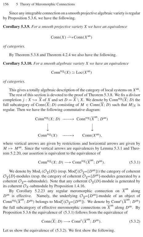
156 5 Theory of Meromorphic Connections
Since any integrable connection on a smooth projective algebraic variety is regularby Proposition 5.3.6, we have the following.
Corollary 5.3.9. For a smooth projective variety X we have an equivalence
Conn(X) −→∼ Conn(Xan)
of categories.
By Theorem 5.3.8 and Theorem 4.2.4 we also have the following.
Corollary 5.3.10. For a smooth algebraic variety X we have an equivalence
Connreg(X) � Loc(Xan)
of categories.
This gives a totally algebraic description of the category of local systems on Xan.The rest of this section is devoted to the proof of Theorem 5.3.8. We fix a divisor
completion j : X ↪→ X of X and set D = X \ X. We denote by Connreg(X; D) thefull subcategory of Conn(X; D) consisting of M ∈ Conn(X; D) such that M|X isregular. Then we have the following commutative diagram:
Connreg(X; D) −−−−→ Connreg(Xan; Dan)⏐⏐ ⏐⏐
Connreg(X) −−−−→ Conn(Xan),
where vertical arrows are given by restrictions and horizontal arrows are given byM �→ Man. Since the vertical arrows are equivalences by Lemma 5.3.1 and Theo-rem 5.2.20, our assertion is equivalent to the equivalence of
Connreg(X; D) −→ Connreg(Xan; Dan). (5.3.1)
We denote by Modc(OX[D]) (resp. Modec(OX
an [Dan])) the category of coherentOX[D]-modules (resp. the category of coherent O
Xan [Dan]-modules generated by a
coherent OX
an -submodule). Note that any coherent OX[D]-module is generated byits coherent OX-submodule by Proposition 1.4.16.
By Corollary 5.2.23 any regular meromorphic connection on Xan
alongDan is effective. Namely, the underlying O
Xan [Dan]-module of an object of
Connreg(Xan; Dan) belongs to Mode
c(OXan [Dan]). We denote by Conne(X
an; Dan)
the full subcategory of effective meromorphic connections on Xan
along Dan. ByProposition 5.3.6 the equivalence of (5.3.1) follows from the equivalence of
Conn(X; D) −→ Conne(Xan; Dan). (5.3.2)
Let us show the equivalence of (5.3.2). We first show the following.
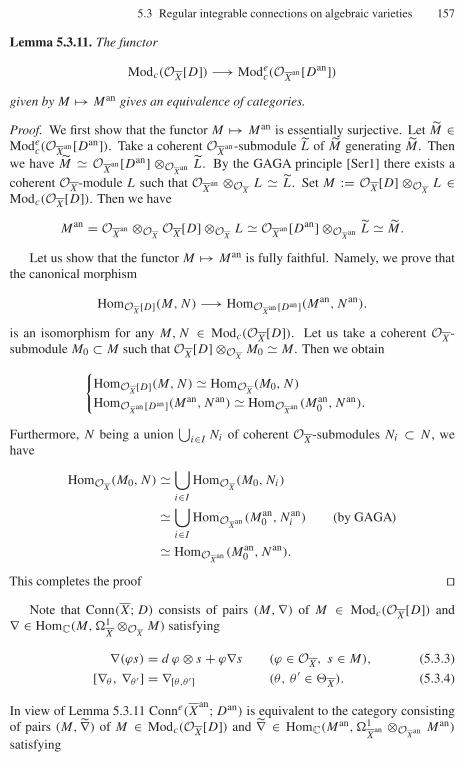
5.3 Regular integrable connections on algebraic varieties 157
Lemma 5.3.11. The functor
Modc(OX[D]) −→ Modec(OX
an [Dan])given by M �→ Man gives an equivalence of categories.
Proof. We first show that the functor M �→ Man is essentially surjective. Let M ∈Mode
c(OXan [Dan]). Take a coherent O
Xan -submodule L of M generating M . Then
we have M � OX
an [Dan] ⊗OX
an L. By the GAGA principle [Ser1] there exists a
coherent OX-module L such that OX
an ⊗OXL � L. Set M := OX[D] ⊗OX
L ∈Modc(OX[D]). Then we have
Man = OX
an ⊗OXOX[D] ⊗OX
L � OX
an [Dan] ⊗OX
an L � M.
Let us show that the functor M �→ Man is fully faithful. Namely, we prove thatthe canonical morphism
HomOX[D](M, N) −→ HomOX
an [Dan](Man, Nan).
is an isomorphism for any M, N ∈ Modc(OX[D]). Let us take a coherent OX-submodule M0 ⊂ M such that OX[D] ⊗OX
M0 � M . Then we obtain{HomOX[D](M, N) � HomOX
(M0, N)
HomOX
an [Dan](Man, Nan) � HomOX
an (Man0 , Nan).
Furthermore, N being a union⋃
i∈I Ni of coherent OX-submodules Ni ⊂ N , wehave
HomOX(M0, N) �
⋃i∈I
HomOX(M0, Ni)
�⋃i∈I
HomOX
an (Man0 , Nan
i ) (by GAGA)
� HomOX
an (Man0 , Nan).
This completes the proof ��Note that Conn(X; D) consists of pairs (M, ∇) of M ∈ Modc(OX[D]) and
∇ ∈ HomC(M, �1X
⊗OXM) satisfying
∇(ϕs) = d ϕ ⊗ s + ϕ∇s (ϕ ∈ OX, s ∈ M), (5.3.3)
[∇θ , ∇θ ′ ] = ∇[θ,θ ′] (θ, θ ′ ∈ �X). (5.3.4)
In view of Lemma 5.3.11 Conne(Xan; Dan) is equivalent to the category consisting
of pairs (M, ∇) of M ∈ Modc(OX[D]) and ∇ ∈ HomC(Man, �1X
an ⊗OX
an Man)
satisfying

158 5 Theory of Meromorphic Connections
∇(ϕs) = d ϕ ⊗ s + ϕ∇s (ϕ ∈ OX
an , s ∈ Man), (5.3.5)
[∇θ , ∇θ ′ ] = ∇[θ,θ ′] (θ, θ ′ ∈ �X
an ). (5.3.6)
Hence it is sufficient to show that for M ∈ Mod(OX[D]) the two sets
� = {∇ ∈ HomC(M, �1X
⊗OXM) | ∇ satisfies (5.3.3) and (5.3.4)},
� = {∇ ∈ HomC(Man, �1X
an ⊗OX
an Man) | ∇ satisfies (5.3.5) and (5.3.6)}are in bijective correspondence. Since these two sets are defined by C-linear mor-phisms (not by O-linear morphisms), we cannot directly use GAGA. We will showthe correspondence by rewriting the conditions in terms of O-linear morphisms.
We first show that the two sets
�1 = {∇ ∈ HomC(M, �1X
⊗OXM) | ∇ satisfies (5.3.3)},
�1 = {∇ ∈ HomC(Man, �1X
an ⊗OX
an Man) | ∇ satisfies (5.3.5)}are in bijective correspondence. We need some preliminaries on differential operators.
Let Y be a complex manifold or a smooth algebraic variety. For OY -modules K
and L we define the subsheaves FpD(K, L) (p ∈ Z) of HomC(M, N) recursivelyon p by FpD(K, L) = 0 for p < 0 and
FpD(K, L) = {P ∈ HomC(M, N) | Pf − f P ∈ Fp−1D(K, L) (∀f ∈ OY )}for p ≥ 0. Sections of FpD(K, L) are called differential operators of order p. Letus give a different description of FpD(K, L). Let δ : Y → Y × Y be the diagonalembedding, and let pj : Y × Y → Y (j = 1, 2) be the projections. We denote byJ ⊂ OY×Y the defining ideal of δ(Y ). By taking δ−1 of the canonical morphismp−1
j OY → OY×Y we obtain two ring homomorphisms
αj : OY = δ−1p−1j OY → δ−1OY×Y
for j = 1, 2. In particular, we have two OY -module structures on δ−1OY×Y . SinceJ is an ideal of OY×Y , we also have two OY -module structures on δ−1J k andδ−1(J k/J l) (k < l). We note that the two OY -module structures onδ−1(J k/J k+1) coincide and that δ−1(J/J 2) is identified with �1
Y . We considerHomOY
(δ−1OY×Y ⊗OYK, L), where the tensor product δ−1OY×Y ⊗OY
K istaken with respect to the OY -module structure on δ−1OY×Y induced by α2, andδ−1OY×Y ⊗OY
K is regarded as an OY -module via the OY -module structure onδ−1OY×Y induced by α1. Define
β : HomOY(δ−1OY×Y ⊗OY
K, L) → HomC(K, L)
by (β(ψ))(s) = ψ(1 ⊗ s). Then we have the following.
Lemma 5.3.12. The morphism β induces an isomorphism
HomOY(δ−1(OY×Y /J p+1) ⊗OY
K, L) � FpD(K, L).

5.3 Regular integrable connections on algebraic varieties 159
The proof is left to the readers.Now we return to the original situation. Note that we have
�1 ⊂ F1D(M, �1X
⊗OXM), �1 ⊂ F1D(Man, �1
Xan ⊗O
Xan Man).
By examining the condition (5.3.3) we see by Lemma 5.3.12 that �1 is in bijectivecorrespondence with the set
{ϕ ∈ HomC(δ−1(OX×X/J 2) ⊗OXM, �1
X⊗OX
M) | ϕ|�1X
⊗OX
M = id},
where δ−1(J/J 2) is identified with �1X
. We have obtained a description of �1 interms of O-modules. The same argument holds true in the analytic category and wehave a similar description of �1. Now we can apply GAGA to conclude that �1 isin bijective correspondence with �1.
Let us finally give a reformulation of the conditions (5.3.4), (5.3.6). For∇ ∈ HomC(M, �1
X⊗OX
M) satisfying (5.3.3) we define ∇1 ∈ HomC(�1X
⊗OX
M, �2X
⊗OXM) by ∇1(ω ⊗ s) = dω ⊗ s − ω ∧ ∇s. Then we have ∇1 ◦ ∇ ∈
HomOX(M, �2
X⊗OX
M), and ∇ satisfies the condition (5.3.4) if and only if
∇1 ◦ ∇ = 0. This gives a reformulation of the condition (5.3.4) in terms of anOX-linear morphism. In the analytic category we also have a similar reformulationof the condition (5.3.6). Now we can apply GAGA to obtain the desired bijection� � �. The proof of Theorem 5.3.8 is now complete.
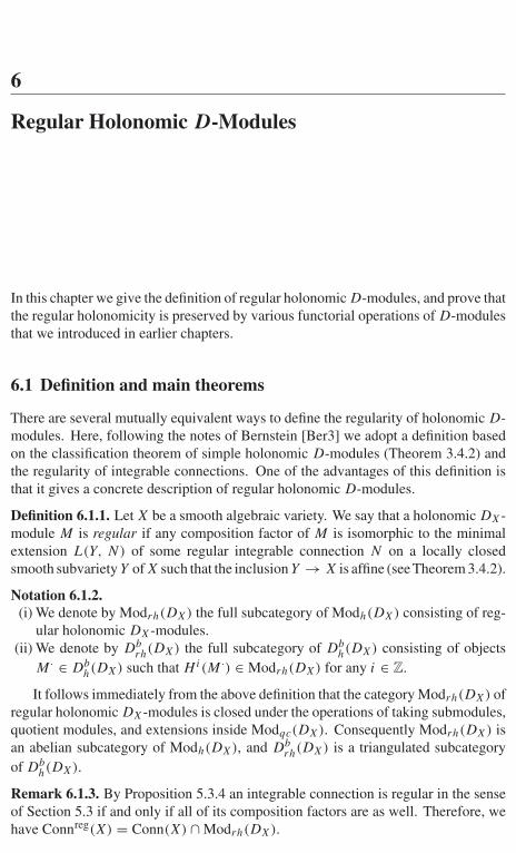
6
Regular Holonomic D-Modules
In this chapter we give the definition of regular holonomic D-modules, and prove thatthe regular holonomicity is preserved by various functorial operations of D-modulesthat we introduced in earlier chapters.
6.1 Definition and main theorems
There are several mutually equivalent ways to define the regularity of holonomic D-modules. Here, following the notes of Bernstein [Ber3] we adopt a definition basedon the classification theorem of simple holonomic D-modules (Theorem 3.4.2) andthe regularity of integrable connections. One of the advantages of this definition isthat it gives a concrete description of regular holonomic D-modules.
Definition 6.1.1. Let X be a smooth algebraic variety. We say that a holonomic DX-module M is regular if any composition factor of M is isomorphic to the minimalextension L(Y, N) of some regular integrable connection N on a locally closedsmooth subvariety Y of X such that the inclusion Y → X is affine (see Theorem 3.4.2).
Notation 6.1.2.(i) We denote by Modrh(DX) the full subcategory of Modh(DX) consisting of reg-
ular holonomic DX-modules.(ii) We denote by Db
rh(DX) the full subcategory of Dbh(DX) consisting of objects
M · ∈ Dbh(DX) such that Hi(M ·) ∈ Modrh(DX) for any i ∈ Z.
It follows immediately from the above definition that the category Modrh(DX) ofregular holonomic DX-modules is closed under the operations of taking submodules,quotient modules, and extensions inside Modqc(DX). Consequently Modrh(DX) isan abelian subcategory of Modh(DX), and Db
rh(DX) is a triangulated subcategoryof Db
h(DX).
Remark 6.1.3. By Proposition 5.3.4 an integrable connection is regular in the senseof Section 5.3 if and only if all of its composition factors are as well. Therefore, wehave Connreg(X) = Conn(X) ∩ Modrh(DX).
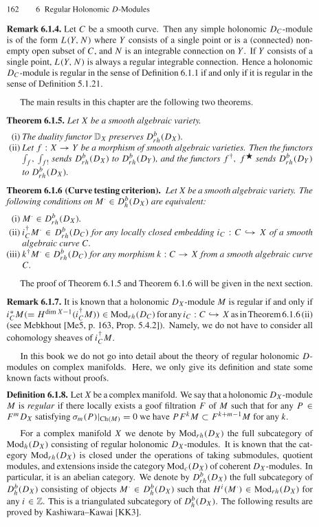
162 6 Regular Holonomic D-Modules
Remark 6.1.4. Let C be a smooth curve. Then any simple holonomic DC-moduleis of the form L(Y, N) where Y consists of a single point or is a (connected) non-empty open subset of C, and N is an integrable connection on Y . If Y consists of asingle point, L(Y, N) is always a regular integrable connection. Hence a holonomicDC-module is regular in the sense of Definition 6.1.1 if and only if it is regular in thesense of Definition 5.1.21.
The main results in this chapter are the following two theorems.
Theorem 6.1.5. Let X be a smooth algebraic variety.
(i) The duality functor DX preserves Dbrh(DX).
(ii) Let f : X → Y be a morphism of smooth algebraic varieties. Then the functors∫f,∫
f ! sends Dbrh(DX) to Db
rh(DY ), and the functors f †, f � sends Dbrh(DY )
to Dbrh(DX).
Theorem 6.1.6 (Curve testing criterion). Let X be a smooth algebraic variety. Thefollowing conditions on M · ∈ Db
h(DX) are equivalent:
(i) M · ∈ Dbrh(DX).
(ii) i†CM · ∈ Db
rh(DC) for any locally closed embedding iC : C ↪→ X of a smoothalgebraic curve C.
(iii) k†M · ∈ Dbrh(DC) for any morphism k : C → X from a smooth algebraic curve
C.
The proof of Theorem 6.1.5 and Theorem 6.1.6 will be given in the next section.
Remark 6.1.7. It is known that a holonomic DX-module M is regular if and only ifi∗CM(= H dim X−1(i
†CM)) ∈ Modrh(DC) for any iC : C ↪→ X as inTheorem 6.1.6 (ii)
(see Mebkhout [Me5, p. 163, Prop. 5.4.2]). Namely, we do not have to consider allcohomology sheaves of i
†CM .
In this book we do not go into detail about the theory of regular holonomic D-modules on complex manifolds. Here, we only give its definition and state someknown facts without proofs.
Definition 6.1.8. Let X be a complex manifold. We say that a holonomic DX-moduleM is regular if there locally exists a goof filtration F of M such that for any P ∈F mDX satisfying σm(P )|Ch(M) = 0 we have PF kM ⊂ F k+m−1M for any k.
For a complex manifold X we denote by Modrh(DX) the full subcategory ofModh(DX) consisting of regular holonomic DX-modules. It is known that the cat-egory Modrh(DX) is closed under the operations of taking submodules, quotientmodules, and extensions inside the category Modc(DX) of coherent DX-modules. Inparticular, it is an abelian category. We denote by Db
rh(DX) the full subcategory ofDb
h(DX) consisting of objects M · ∈ Dbh(DX) such that Hi(M ·) ∈ Modrh(DX) for
any i ∈ Z. This is a triangulated subcategory of Dbh(DX). The following results are
proved by Kashiwara–Kawai [KK3].
6.2 Proof of main theorems 163
Theorem 6.1.9. Let X be a complex manifold. Then any regular holonomic DX-module admits a global good filtration.
Theorem 6.1.10. Let X be a complex manifold. Then the duality functor DX sendsDb
rh(DX) to Dbrh(DX)op.
Theorem 6.1.11. Let f : X → Y be a morphism of complex manifolds.
(i) The inverse image functor f † sends Dbrh(DY ) to Db
rh(DX).(ii) If f is proper, the direct image functor
∫f
sends Dbrh(DX) to Db
rh(DY ).
One can show the following using a result in Kashiwara–Kawai [KK3].
Theorem 6.1.12. Let X be a smooth algebraic variety, and let M be a holonomicDX-module. Take a divisor completion j : X ↪→ X of X. Then M is regular if andonly if (j∗M)an is regular.
6.2 Proof of main theorems
In this section we give a proof of Theorem 6.1.5 and Theorem 6.1.6. It is divided intoseveral steps.
(Step 1) We show that the conditions (ii) and (iii) in Theorem 6.1.6 are equivalent.We only need to show that (ii) implies (iii). Assume (ii). Let k : C → X
be a morphism from a smooth algebraic curve C. We may assume that C is con-nected. If Im(k) consists of a single point p, then we have k†M · � OC ⊗C r†M ·[1],where r : {p} ↪→ X is the inclusion. Hence the assertion is obvious. Assumethat dim Im(k) = 1. Take a non-empty smooth open subset C′ of Im(k) anddenote by k0 : C0 := k−1C′ → C′ the canonical morphism. Then we havek†M ·|C0 = k
†0i
†C′M · ∈ Db
rh(DC0) by (ii) and Lemma 5.1.23. Hence we obtaink†M · ∈ Db
rh(DC) by Remark 6.1.4.
(Step 2) Let us show Theorem 6.1.5 (i).We need to show DXM · ∈ Db
rh(DX) for M · ∈ Dbrh(DX). By induction on the
cohomological length of M · we may assume that M · = M ∈ Modrh(DX). We canalso reduce the problem to the case when M is simple by induction on the length ofthe composition series of M . In this case M is the minimal extension L(Y, N) of aregular integrable connection N on a locally closed smooth subvariety Y of X suchthat the inclusion i : Y → X is affine. By Proposition 3.4.3 and Example 2.6.10we have
DXL(Y, N) � L(Y, DY N), DY N � HomOY(N, OY ).
Hence the assertion is a consequence of Proposition 5.3.5. The proof of Theo-rem 6.1.5 (i) is complete.
It follows from Step 2 that the proof of Theorem 6.1.5 (ii) is reduced to thefollowing two statements for a morphism f : X → Y of smooth algebraic varieties:
164 6 Regular Holonomic D-Modules
(a) For any M · ∈ Dbrh(DX) we have
∫f
M · ∈ Dbrh(DY ).
(b) For any M · ∈ Dbrh(DY ) we have f †M · ∈ Db
rh(DX).
We first verify (a) in some special cases in Step 3 and Step 4.
(Step 3) Let X be a smooth algebraic variety and let X be a smooth completion of X
such that the complementary set D = X \ X is a normal crossing divisor on X. Weshow that (a) holds when f is the embedding j : X ↪→ X and M · = M ∈ Connreg(X).
The functor j∗ being exact, we may assume that M is simple by induction on thelength of M . By Theorem 3.4.2 (ii), each composition factor L of j∗M is of the formL = L(Y, N) (Y ⊂ X is affine and N is an integrable connection on Y ), and we needto show that N is a regular integrable connection. If j†L = 0, then we have N � M
by Theorem 3.4.2, and hence N is regular in this case. Therefore, we assume thatj†L = 0 in the following.
Claim. Let D = X \X = ⋃ri=1 Di be the irreducible decomposition of D. For each
subset I ⊂ {1, 2, . . . , r} set DI := ⋂i∈I
Di and consider its irreducible decomposition
DI = ⋃α DI,α . Also set D′
I,α := DI,α \ ⋃j /∈I
Dj (an open subset of DI,α). Then
for the above composition factor L satisfying j†L = 0, there exist a pair (I, α) withI = ∅ and an integrable connection N over D′
I,α such that L � L(D′I,α, N).
Proof of claim. Theorem 5.3.7 implies that j∗M is generated by a �X〈D〉-stablecoherent OX-submodule K . Define a good filtration F of j∗M by Fp(j∗M) =(FpDX)K for p ≥ 0. Then �X〈D〉(⊂ �X = grF
1 DX) acts trivially on grF M .From this we easily see that
Ch(j∗M) ⊂⋃I,α
T ∗DI,α
X.
In other words, the characteristic variety Ch(j∗M) is a union of conormal bundlesT ∗
DI,αX. Since Ch(L) ⊂ Ch(j∗M), L must satisfy the same condition. Therefore, the
support of L is a union of DI,α’s. Let us take an irreducible component DI,α of thesupport of L. Let iD′
I,α: D′
I,α → X be the inclusion. By Kashiwara’s equivalence and
Lemma 2.3.5 we see that the characteristic variety of the pull-back N := (iD′I,α
)†L to
D′I,α coincides with the zero-section T ∗
D′I,α
D′I,α , and hence N is a non-zero integrable
connection by Proposition 2.2.5. By (the proof of) Theorem 3.4.2 (ii) we easily seefrom the simplicity of L that L coincides with the minimal extension L(D′
I,α, N)
of N . ��Now our task is to prove that the integrable connection N in the claim above is
regular. By Theorem 5.3.7 we have j∗M = ⋃i Wi for coherent OX-submodules Wi
of j∗M stable under the action of DX[D]. Hence the composition factor L of j∗M
also satisfies the same condition L = ⋃i W ′
i . Note that the pair (D′I,α, DI,α) is geo-
metrically very similar to (X, X), and that �I,α := DI,α \ D′I,α is a normal crossing
6.2 Proof of main theorems 165
divisor on DI,α . Now recall that supp L = DI,α . Therefore, by Kashiwara’s equiv-alence for the inclusion iDI,α
: DI,α ↪→ X, the complex (iDI,α)†L is concentrated in
degree 0.Let us show that (iDI,α
)†L also satisfies the same property as L itself, thatis, (iDI,α
)†L is a union of coherent ODI,α-submodules stable under the action of
DDI,α[�I,α]. First consider the case where X ⊃ D = {x1 · · · xr = 0} ⊃ DI =
{x1 = 0}. Then we have H 0(iDI)†L = Ker(x1 : L → L) and the coherent OX-
submodule W ′i stable under the actions of θi = xi∂i (1 ≤ i ≤ r) induces a coherent
ODI-coherent submodule Vi = W ′
i ∩ Ker(x1 : L → L) of (iDI)†L stable under the
actions of θi (2 ≤ i ≤ r). We also have (iDI)†L = ⋃
i Vi . In the general case wherethe codimension of DI,α is greater than one we can repeat this procedure.
Now let h = 0 be the defining equation of the divisor �I,α on DI,α . Then wesee that
(iD′I,α↪→DI,α
)∗N = ODI,α[�I,α] ⊗ODI,α
(iDI,α)†L
also has the same property⋃
k≥0, i
[ODI,αh−k ⊗ Vi] = ODI,α
[�I,α] ⊗ODI,α(iDI,α
)†L.
Therefore, Theorem 5.3.7 implies that N is a regular connection on D′I,α .
(Step 4) For an algebraic variety Y we denote the singular locus of Y by Sing Y . Weshow the following.
Claim. Let S (resp. C) be a smooth projective algebraic variety of dimension 2 (resp.1), and let S0 ⊂ S (resp. C0 ⊂ C) be a non-empty open subset. Set �S := S \S0 and�C := C \C0. We assume that �S is a normal crossing divisor on S. Let f : S → C
be a morphism satisfying the following conditions:
(i) f (S0) ⊂ C0 and f |S0 : S0 → C0 is smooth.(ii) f (Sing �S) ⊂ �C .
We denote by i : S0 ↪→ S the embedding. Then for any regular integrable connectionM on S0 we have
∫f
i∗M ∈ Dbrh(DC).
This result is due to Griffiths [Gri] and it was later generalized to higher dimensionsby Deligne. We call this fact the regularity of Gauss–Manin connections.
Proof of claim. Recall the notation DS〈�S〉, DC〈�C〉, etc., in Section 5.3. Similarlyto DS→C , we define a (DS〈�S〉, f −1DC〈�C〉)-bimodule DS→C〈�〉 by
DS→C〈�〉 := OS ⊗f −1OCf −1DC〈�C〉.
For the sake of simplicity we consider the corresponding equivalent problem in thecategory of “right’’ D-modules. Recall that the direct image under f of a complexM · ∈ Db(D
opS ) of right DS-modules is given by∫
f
M · := Rf∗(M · ⊗LDS
DS→C).
We define a functor
166 6 Regular Holonomic D-Modules∫ 〈�〉
f
: Db(Mod(DS〈�S〉op)) −→ Db(Mod(DC〈�C〉op))
by ∫ 〈�〉
f
M · := Rf∗(M · ⊗LDS 〈�S 〉 DS→C〈�〉).
Then we have
(1) For M ∈ Mod(DopS0
) we have an isomorphism∫f
i∗M �∫ 〈�〉
f
i∗M
in Db(Mod(DC〈�C〉op)).(2) Let L be a right DS〈�S〉-module which is coherent over OS . Then all the co-
homology sheaves of∫ 〈�〉
fL are right DC〈�C〉-modules which are coherent
over OC .
The assertion (1) follows immediately from DS〈�S〉|S0 = DS0 and DS→C〈�〉|S0= DS0→C0 . Let us prove (2). By our conditions (i), (ii) on f we see that the canonicalmorphism
�S〈�S〉 −→ f ∗�C〈�C〉 = OS ⊗f −1OCf −1�C〈�C〉
is an epimorphism. Denote by �S/C〈�〉 its kernel. Then we have an exact sequence
0 −→ DS〈�S〉 ⊗OS�S/C〈�〉 −→ DS〈�S〉 −→ DS→C[�] −→ 0
of DS〈�S〉-modules. We can regard this as a locally free resolution of DS→C〈�〉,and hence for a right DS〈�S〉-module L we have∫ 〈�〉
f
L = Rf∗[L ⊗OS
�S/C〈�〉 −→ L].
Since f is proper, the cohomology sheaves H ∗(∫ 〈�〉
fL) are coherent over OC if L is
coherent over OS . This completes the proof of (2).Now we can finish the proof of our claim. Since M is a regular integrable connec-
tion on S0, we see by Theorem 5.3.7 that there exist OS-coherent DS〈�S〉-submodulesLα ⊂ i∗M such that i∗M = lim−→
α
Lα . By (1) there exist isomorphisms
H ∗∫
f
i∗M � H ∗∫ 〈�〉
f
i∗M � H ∗∫ 〈�〉
f
lim−→α
Lα � lim−→α
H ∗∫ 〈�〉
f
Lα
of DC〈�C〉-modules. By (2) H ∗(∫ 〈�〉
fLα) is coherent over OC , and hence we have∫
fi∗M ∈ Db
rh(DC) by Theorem 5.3.7. The proof of our claim is complete. ��In Step 5–Step 8 we will show the statement (a) and the equivalence of (i) and (ii)
in Theorem 6.1.6 simultaneously by induction on dim supp(M ·), where supp(M ·) :=⋃j supp(Hj (M ·)).
6.2 Proof of main theorems 167
(Step 5) We show that the statement (a) holds when f is an affine embedding i :X ↪→ Y and M = M · ∈ Connreg(X).
Let us consider the distinguished triangle∫i!
M −→∫
i
M −→ Ci(M)+1−→
in Dbh(DY ) associated to the morphism
∫i! → ∫
i(see Section 3.4). Since i is an
affine embedding, we have Hp∫
iM = 0 (p = 0) and Hp
∫i! M = 0 (p = 0).
Therefore, by considering the cohomology long exact sequence associated to theabove distinguished triangle we see that any composition factor of H 0(
∫i! M) or
H 0(∫
iM) is isomorphic to that of H ∗Ci(M) or to that of the minimal extension
L(X, M) = Im(H 0(
∫i! M) → H 0(
∫iM)). Since L(X, M) is regular by definition,
we have only to show that Ci(M) ∈ Dbrh(DY ).
By a theorem of Hironaka we can decompose the morphism i into the compositeof an open immersion j : X → X and a proper morphism f : X → Y , whereX \ X is a normal crossing divisor on X. By applying the functor
∫f
= ∫f ! to the
distinguished triangle ∫j !
M −→∫
j
M −→ Cj (M)+1−→
associated to the open embedding j we obtain a distinguished triangle∫i!
M −→∫
i
M −→∫
f
Cj (M)+1−→ .
Hence we have∫
fCj (M) � Ci(M). On the other hand we know already that∫
jM,
∫j ! M ∈ Db
rh(DX) by Step 2 and Step 3. Hence it follows from the above
distinguished triangle that Cj (M) ∈ Dbrh(DX). Moreover, by the construction in
Theorem 3.4.2 we have
dim supp Cj (M) < dim supp M.
Therefore, we obtain Ci(M) � ∫f
Cj (M) ∈ Dbrh(DY ) by our hypothesis of induction.
(Step 6) We give a proof of (i)=⇒(ii) in Theorem 6.1.6, i.e., we show i†CM · ∈
Dbrh(DC) for any M · ∈ Db
rh(DX) and any embedding iC : C ↪→ X of an algebraiccurve.
By induction on the cohomological length of M · we may assume M · = M ∈Modrh(DX). We may also assume that M is a simple object of Modrh(DX) byinduction on the length of M . In this case M is a minimal extension M = L(Y, N)
(j : Y ↪→ X: affine) of a simple regular integrable connection N on Y . Set Q =(∫
jN)/M . By Theorem 3.4.2 we have dim supp Q < dim supp M . Moreover, we
have Q ∈ Dbrh(DX) by Step 5. Therefore, the hypothesis of induction implies that
we have i†CQ ∈ Db
rh(DC). Hence by the distinguished triangle

168 6 Regular Holonomic D-Modules
i†CM −→ i
†C
∫j
N −→ i†CQ
+1−→
we have only to show i†C
∫j
N ∈ Dbrh(DC). By applying the base change theorem
(Theorem 1.7.3) to the cartesian square
Y ∩ Ci0→ Y
j0
−→
j
↪−→C
iC↪→ X,
we get i†C
∫j
N � ∫j0
i†0N (note that Y ∩ C is smooth since C is one-dimensional).
Hence it is sufficient to show that∫
j0i†0N ∈ Db
rh(DC). In the case dim Y ∩ C = 0this is obvious. If dim Y ∩ C = 1, then Y ∩ C is an open subset of C. In this casei†0N is a regular integrable connection on Y ∩C up to a shift of degrees by definition.
Hence by the definition of regular holonomic D-modules on algebraic curves, wehave
∫j0
i†0N ∈ Db
rh(DC).
(Step 7) We give a proof of (ii)=⇒(i) in Theorem 6.1.6.
Let M · ∈ Dbh(DX). We assume that i
†CM · ∈ Db
rh(DC) for any embeddingiC : C ↪→ X of an algebraic curve, and will show that M · ∈ Db
rh(DX). SetS = supp M ·. By Proposition 3.1.6 there exists an open dense subset Y of S suchthat H ∗(i†M ·) are integrable connections on Y (i : Y ↪→ X). We may assume thati : Y ↪→X is an affine embedding. Take an open dense subset U of X such thatS ∩ U = Y and set Z = X \ U . We denote by k : Y → U and j : U → X theembeddings. Note that i = j ◦ k and that j (resp. k) is an open (resp. a closed)embedding. By the distinguished triangle
R�Z(M ·) −→ M · −→∫
j
j†M · +1−→
in Dbh(DX) associated to the triplet U ↪→ X ←↩ Z it is sufficient to show that
R�Z(M ·),∫
jj†M · ∈ Db
rh(DX).
We first show R�Z(M ·) ∈ Dbrh(DX). By supp R�Z(M ·) ⊂ S ∩ Z we have
dim supp R�Z(M ·) < dim supp M ·. Hence we have only to show to i†CR�Z(M ·) ∈
Dbrh(DC) for any curve C by the hypothesis of induction. Applying the functor i
†C to
the above distinguished triangle we obtain a distinguished triangle
i†CR�Z(M ·) −→ i
†CM · −→ i
†C
∫j
j†M · +1−→
Hence it is sufficient to show i†C
∫j
j†M · ∈ Dbrh(DX). By applying the base change
theorem to the cartesian square
6.2 Proof of main theorems 169
Uj−−−−→ X�⏐⏐ iC
�⏐⏐U ∩ C
α−−−−→ C
we obtain i†C
∫j
j†M · � ∫α
α†i†CM ·, and hence we have only to show that∫
αα†i
†CM · ∈ Db
rh(DC). This is obvious if dim U ∩ C = 0. Assume that
dim U ∩ C = 1. By our assumption we have i†CM · ∈ Db
rh(DC), and hence we
obtain∫
αα†i
†CM · ∈ Db
rh(DC) by the definition of the regularity for holonomicD-modules on algebraic curves.
Next let us show∫
jj†M · ∈ Db
rh(DX). By applying Kashiwara’s equivalence
(Theorem 1.6.2) to the closed embedding k : Y ↪→ U we easily see that∫
jj†M · �∫
ii†M ·. Recall that H ∗(i†M ·) are integrable connections on Y . Since i is affine, it
is sufficient to show H ∗(i†M ·) ∈ Connreg(Y ) by Step 5. For this it is sufficient toshow j
†CH ∗(i†M ·) ∈ Db
rh(DC) for any locally closed embedding jC : C → Y of a
curve C into Y . Since H ∗(i†M ·) are integrable connections, we have j†CH ∗(i†M ·) �
H ∗−1+dY (j†Ci†M ·)[1 − dY ] � H ∗−1+dY ((i ◦ jC)†M ·)[1 − dY ]. Hence it belongs to
Dbrh(DC) by our assumption on M ·.
(Step 8) We give a proof of (a) for general f .It is enough to prove the assertion separately for the case of closed embeddings,
and for the case of projections.We first treat the case when f : X → Y is a closed embedding. As before we
may assume that M · = M = L(X1, N) for some locally closed smooth subvarietyX1 of X such that the embedding i : X1 → X is affine and N ∈ Connreg(X1). Sincethe dimension of the support of the cokernel of the morphism L(X1, N) ↪→ ∫
iN is
less than that of M · = L(X1, N), it is enough to prove∫
f ◦iN ∈ Db
rh(DY ) by ourhypothesis of induction. This assertion has already been proved in Step 5 (f ◦ i is anaffine embedding).
Next we deal with the case of a projection f : X = Z × Y → Y and M · ∈Db
rh(DX). By the argument in the proof of Lemma 3.2.5 we may assume that Z isaffine from the beginning. Let us choose a closed embedding j : Z → AN andfactorize f as the composite of j × IdY : X = Z × Y → AN × Y and a projectionAN × Y → Y . Since the morphism j × IdY is a closed embedding, it is enough toprove our assertion for p : AN × Y → Y . Moreover, decomposing AN × Y → Y
into AN × Y → AN−1 × Y → · · · → A1 × Y → Y , we can further reduce theproblem to the case of projections A1 × Y → Y (with fiber A1). By Step 6, Step 7,and Theorem 1.7.3 we may also assume that Y is an algebraic curve C. Namely, forp : A1 ×C → C and M · ∈ Db
rh(DA1×C), we have only to prove∫
pM · ∈ Db
rh(DC).As before, we may assume that M · = M = L(X1, N) for some locally closed smoothsubvariety X1 of A1 × C such that i : X1 → A1 × C is affine and N ∈ Connreg(X1).By dim supp Coker(L(X1, N) → ∫
iN) < dim supp(L(X1, N) and the hypothesis
of induction it is sufficient to show∫
p◦iN ∈ Db
rh(DC). The case dim X1 ≤ 1 is
170 6 Regular Holonomic D-Modules
already known (see Lemma 5.1.23) and hence we may assume that X1 is an opensubset of A1 × C. Namely, it is sufficient to show following statement.
Claim. Let U be a non-empty open subset of A1 ×C. We denote by i : U → A1 ×C
and p : A1 × C → C the embedding and the projection, respectively. Then for anyregular integrable connection N on U we have
∫p◦i
N ∈ Dbrh(DC).
Proof of claim. We first note that we can always replace C and U with a non-emptyopen dense subset C′ of C and U ′ = p−1C′ ∩ U , respectively, by the definition ofregularity for holonomic D-modules on algebraic curves. Take a smooth completionj : C → C of C, and regard A1 × C as an open subset of P1 × C. We denote byp : P1 × C → C the projection. Note that (P1 × C) \ U is a union of a divisorand finitely many points. Hence by replacing C with its non-empty open subsetwe may assume from the beginning that p(Sing((P1 × C) \ U)) ⊂ C \ C. Thenby Hironaka’s desingularization theorem we can take a proper surjective morphismπ : S → P1 × C such that the morphism π0 : π−1(U) → U induced by π is anisomorphism, �S := π−1((P1 × C) \ U) is a normal crossing divisor on S, andπ(Sing �S) ⊂ Sing((P1 × C) \ U). Set S0 = π−1U , f = p ◦ π : S → C, and leti : S0 → S be the embedding. Then we have f (Sing � = S) ⊂ C \ C, and
j∗∫
p◦i
N �∫
f
i∗π∗0 N.
Hence our claim follows from Step 4. ��(Step 9) The statement (b) follows easily from Theorem 6.1.6.
The proof of Theorem 6.1.5 and Theorem 6.1.6 is now complete.
7
Riemann–Hilbert Correspondence
This chapter is concerned with one of the most important theorems in D-moduletheory. This fundamental theorem, which is now called the Riemann–Hilbert cor-respondence, establishes an equivalence between the category of regular holonomicD-modules and that of perverse sheaves. It builds a bridge from analysis to topologyleading us to a number of applications in various fields in mathematics.
7.1 Commutativity with de Rham functors
Recall that for a smooth algebraic variety X we have the duality functors
DX : Dbh(DX) → Db
h(DX)op, DX : Dbc (X) → Db
c (X)op.
Recall also that for a morphism f : X → Y of smooth algebraic varieties we havethe functors ∫
f
: Dbh(DX) −→ Db
h(DY ), Rf∗ : Dbc (X) −→ Db
c (Y ),∫f !
: Dbh(DX) −→ Db
h(DY ), Rf! : Dbc (X) −→ Db
c (Y ),
f † : Dbh(DY ) −→ Db
h(DX), f ! : Dbc (Y ) −→ Db
c (X),
f � : Dbh(DY ) −→ Db
h(DX), f −1 : Dbc (Y ) −→ Db
c (X).
By Theorem 6.1.5 all of the functors DX,∫
f,∫
f !, f †, f � preserve Dbrh. We know
already that
DX DRX(M ·) � DRX(DXM ·) (M · ∈ Dbh(DX)) (7.1.1)
(see Corollary 4.6.5 and Proposition 4.7.9), i.e., the de Rham functor on Dbh commutes
with the duality functors. In this section we will also prove the commutativity of thede Rham functor on Db
rh with the inverse and direct image functors.
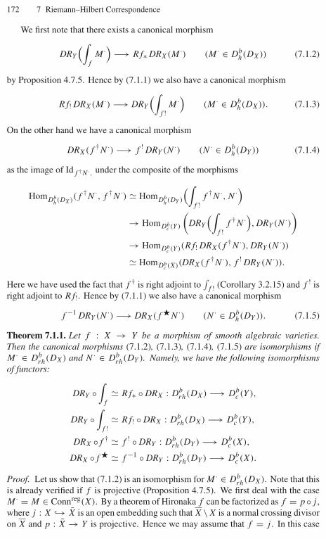
172 7 Riemann–Hilbert Correspondence
We first note that there exists a canonical morphism
DRY
(∫f
M ·) −→ Rf∗ DRX(M ·) (M · ∈ Dbh(DX)) (7.1.2)
by Proposition 4.7.5. Hence by (7.1.1) we also have a canonical morphism
Rf! DRX(M ·) −→ DRY
(∫f !
M ·) (M · ∈ Dbh(DX)). (7.1.3)
On the other hand we have a canonical morphism
DRX(f †N ·) −→ f ! DRY (N ·) (N · ∈ Dbh(DY )) (7.1.4)
as the image of Idf †N ·, under the composite of the morphisms
HomDbh(DX)(f
†N ·, f †N ·) � HomDbh(DY )
(∫f !
f †N ·, N ·)→ HomDb
c (Y )
(DRY
(∫f !
f †N ·), DRY (N ·))
→ HomDbc (Y )(Rf! DRX(f †N ·), DRY (N ·))
� HomDbc (X)(DRX(f †N ·), f ! DRY (N ·)).
Here we have used the fact that f † is right adjoint to∫
f ! (Corollary 3.2.15) and f ! isright adjoint to Rf!. Hence by (7.1.1) we also have a canonical morphism
f −1 DRY (N ·) −→ DRX(f �N ·) (N · ∈ Dbh(DY )). (7.1.5)
Theorem 7.1.1. Let f : X → Y be a morphism of smooth algebraic varieties.Then the canonical morphisms (7.1.2), (7.1.3), (7.1.4), (7.1.5) are isomorphisms ifM · ∈ Db
rh(DX) and N · ∈ Dbrh(DY ). Namely, we have the following isomorphisms
of functors:
DRY ◦∫
f
� Rf∗ ◦ DRX : Dbrh(DX) −→ Db
c (Y ),
DRY ◦∫
f !� Rf! ◦ DRX : Db
rh(DX) −→ Dbc (Y ),
DRX ◦f † � f ! ◦ DRY : Dbrh(DY ) −→ Db
c (X),
DRX ◦f � � f −1 ◦ DRY : Dbrh(DY ) −→ Db
c (X).
Proof. Let us show that (7.1.2) is an isomorphism for M · ∈ Dbrh(DX). Note that this
is already verified if f is projective (Proposition 4.7.5). We first deal with the caseM · = M ∈ Connreg(X). By a theorem of Hironaka f can be factorized as f = p◦j ,where j : X ↪→ X is an open embedding such that X \X is a normal crossing divisoron X and p : X → Y is projective. Hence we may assume that f = j . In this case
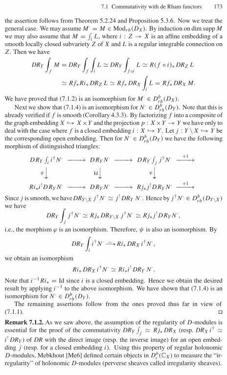
7.1 Commutativity with de Rham functors 173
the assertion follows from Theorem 5.2.24 and Proposition 5.3.6. Now we treat thegeneral case. We may assume M · = M ∈ Modrh(DX). By induction on dim supp M
we may also assume that M = ∫iL, where i : Z → X is an affine embedding of a
smooth locally closed subvariety Z of X and L is a regular integrable connection onZ. Then we have
DRY
∫f
M = DRY
∫f
∫i
L � DRY
∫f ◦i
L � R(f ◦ i)∗ DRZ L
� Rf∗Ri∗ DRZ L � Rf∗ DRX
∫i
L = Rf∗ DRX M.
We have proved that (7.1.2) is an isomorphism for M · ∈ Dbrh(DX).
Next we show that (7.1.4) is an isomorphism for N · ∈ Dbrh(DY ). Note that this is
already verified if f is smooth (Corollary 4.3.3). By factorizing f into a composite ofthe graph embedding X ↪→ X×Y and the projection p : X×Y → Y we have only todeal with the case where f is a closed embedding i : X ↪→ Y . Let j : Y \X ↪→ Y bethe corresponding open embedding. Then for N · ∈ Db
rh(DY ) we have the followingmorphism of distinguished triangles:
DRY
∫ii†N · −−−−→ DRY N · −−−−→ DRY
∫j
j†N · +1−−−−→ψ
⏐⏐ Id
⏐⏐ ϕ
⏐⏐Ri∗i!DRY N · −−−−→ DRY N · −−−−→ Rj∗j !DRY N · +1−−−−→
Since j is smooth, we have DRY\X j†N · � j ! DRY N ·. Hence by j†N · ∈ Dbrh(DY\X)
we have
DRY
∫j
j†N · � Rj∗ DRY\X j†N · � Rj∗j !DRY N ·,
i.e., the morphism ϕ is an isomorphism. Therefore, ψ is also an isomorphism. By
DRY
∫i
i†N · −→∼ Ri∗ DRX i†N ·,
we obtain an isomorphism
Ri∗ DRX i†N · � Ri∗i! DRY N ·.Note that i−1Ri∗ = Id since i is a closed embedding. Hence we obtain the desiredresult by applying i−1 to the above isomorphism. We have shown that (7.1.4) is anisomorphism for N · ∈ Db
rh(DY ).The remaining assertions follow from the ones proved thus far in view of
(7.1.1). ��Remark 7.1.2. As we saw above, the assumption of the regularity of D-modules isessential for the proof of the commutativity DRY
∫j
� Rj∗ DRX (resp. DRX i† �i! DRY ) of DR with the direct image (resp. the inverse image) for an open embed-ding j (resp. for a closed embedding i). Using this property of regular holonomicD-modules, Mebkhout [Me6] defined certain objects in Db
c (CX) to measure the “ir-regularity’’ of holonomic D-modules (perverse sheaves called irregularity sheaves).
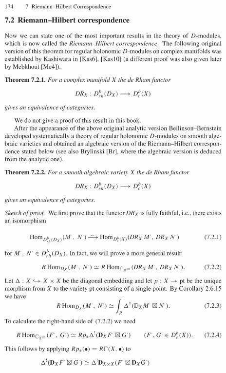
174 7 Riemann–Hilbert Correspondence
7.2 Riemann–Hilbert correspondence
Now we can state one of the most important results in the theory of D-modules,which is now called the Riemann–Hilbert correspondence. The following originalversion of this theorem for regular holonomic D-modules on complex manifolds wasestablished by Kashiwara in [Kas6], [Kas10] (a different proof was also given laterby Mebkhout [Me4]).
Theorem 7.2.1. For a complex manifold X the de Rham functor
DRX : Dbrh(DX) −→ Db
c (X)
gives an equivalence of categories.
We do not give a proof of this result in this book.After the appearance of the above original analytic version Beilinson–Bernstein
developed systematically a theory of regular holonomic D-modules on smooth alge-braic varieties and obtained an algebraic version of the Riemann–Hilbert correspon-dence stated below (see also Brylinski [Br], where the algebraic version is deducedfrom the analytic one).
Theorem 7.2.2. For a smooth algebraic variety X the de Rham functor
DRX : Dbrh(DX) −→ Db
c (X)
gives an equivalence of categories.
Sketch of proof. We first prove that the functor DRX is fully faithful, i.e., there existsan isomorphism
HomDbrh(DX)(M
·, N ·) −→∼ HomDbc (X)(DRX M ·, DRX N ·) (7.2.1)
for M ·, N · ∈ Dbrh(DX). In fact, we will prove a more general result:
R HomDX(M ·, N ·) � R HomCXan (DRX M ·, DRX N ·). (7.2.2)
Let � : X ↪→ X × X be the diagonal embedding and let p : X → pt be the uniquemorphism from X to the variety pt consisting of a single point. By Corollary 2.6.15we have
R HomDX(M ·, N ·) �
∫p
�†(DXM · � N ·). (7.2.3)
To calculate the right-hand side of (7.2.2) we need
R HomCXan (F ·, G·) � Rp∗�!(DXF · � G·) (F ·, G· ∈ Dbc (X)). (7.2.4)
This follows by applying Rp∗(•) = R�(X, •) to
�!(DXF · � G·) � �!DX×X(F · � DXG·)
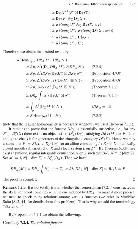
7.2 Riemann–Hilbert correspondence 175
� DX�−1(F · � DXG·)� DX(F · ⊗C DXG·)� RHomC(F · ⊗C DXG·, ωX)
� RHomC(F ·, RHomC(DXG·, ωX))
� RHomC(F ·, D2XG·)
� RHomC(F ·, G·).
Therefore, we obtain the desired result by
R HomCXan (DRX M ·, DRX N ·)� Rp∗�!((DX DRX M ·) � DRX N ·) (7.2.4)
� Rp∗�!(DRX(DXM ·) � DRX N ·) (Proposition 4.7.9)
� Rp∗�!(DRX×X((DXM ·) � N ·)) (Proposition 4.7.8)
� Rp∗ DRX(�†(DXM · � N ·)) (Theorem 7.1.1)
� DRpt
∫p
�†(DXM · � N ·) (Theorem 7.1.1)
�∫
p
�†(DXM · � N ·) (DRpt = Id)
� R HomDX(M ·, N ·) (7.2.3)
(note that the regular holonomicity is necessary whenever we used Theorem 7.1.1).It remains to prove that the functor DRX is essentially surjective, i.e., for any
F · ∈ Dbc (X) there exists an object M · ∈ Db
rh(DX) satisfying DRX(M ·) � F ·. It isenough to check it for generators of the triangulated category Db
c (X). Hence we mayassume that F · = Ri∗L ∈ Db
c (CX) for an affine embedding i : Z ↪→ X of a locallyclosed smooth subvariety Z of X and a local system L on Zan. By Theorem 5.3.8 thereexists a (unique) regular integrable connection N on Z such that DRZ N � L[dim Z].Set M · = ∫
iN [− dim Z] ∈ Db
rh(DX). Then we have
DRX(M ·) = DRX
∫i
N [− dim Z] � Ri∗ DRZ N [− dim Z] � Ri∗L = F ·.
The proof is complete. ��Remark 7.2.3. It is not totally trivial whether the isomorphism (7.2.1) constructed inthe sketch of proof coincides with the one induced by DRX. To make it more precise,we need to check many relations among various functors (we refer to MorihikoSaito [Sa2, §4] for details about this problem). That is why we add the terminology“Sketch of.’’
By Proposition 4.2.1 we obtain the following.
Corollary 7.2.4. The solution functor
176 7 Riemann–Hilbert Correspondence
SolX : Dbrh(DX) −→∼ Db
c (X)op
gives an equivalence of categories.
The image of the full subcategory Modrh(DX) of Dbrh(DX) under the de Rham
functor DRX : Dbrh(DX)
∼→ Dbc (X) is described by the following.
Theorem 7.2.5. The de Rham functor induces an equivalence
DRX : Modrh(DX) −→∼ Perv(CX)
of categories. In particular, Perv(CX) is an abelian category.
The rest of this section is devoted to the proof of Theorem 7.2.5.For n ∈ Z we denote by D
≥nh (DX) (resp. D
≤nh (DX)) the full subcategory of
Dbh(DX) consisting of M · satisfying Hj (M ·) = 0 for j < n (resp. j > n). We also
define full subcategories D≥nc (X) and D≤n
c (X) of Dbc (X) similarly.
Lemma 7.2.6. For M · ∈ Dbh(DX) we have
M · ∈ D≥0h (DX) ⇐⇒ DXM · ∈ D
≤0h (DX).
Proof. Let us show (=⇒). We may assume that M · = 0. Let j be the smallest(non-negative) integer such that Hj (M ·) = 0. Then we have a distinguished triangle
Hj (M ·)[−j ] −→ M · −→ τ�j+1M · +1−→ .
Hence by induction on the cohomological length of M · it is sufficient to showDX(N [−j ]) ∈ Db
h(DX) for any N ∈ Modh(DX) and any non-negative integerj . This follows from DX(N [−j ]) = DX(N)[j ] and Corollary 2.6.8 (iii). The proofof (⇐=) is similar. ��Corollary 7.2.7. An object M · of Db
h(DX) belongs to Modh(DX) if and only if both
M · and DXM · belong to D≥0h (DX).
Lemma 7.2.8. The following conditions on M · ∈ Dbh(DX) are equivalent:
(i) M · ∈ D≥0h (DX).
(ii) For any locally closed subvariety Y of X there exists a smooth open dense subsetY0 of Y such that i
†Y0
M · ∈ D≥0h (DY0) and Hj (i
†Y0
M ·) is coherent over OY0 forany j , where iY0 : Y0 → X denotes the embedding.
Proof. (i) ⇒ (ii): In view of Proposition 3.1.6 it is sufficient to show that for anysmooth open dense subset Y0 of Y we have i
†Y0
M · ∈ D≥0h (DY0). This follows from
the fact that the right i−1Y0
DX-module DY0→X locally admits a free resolution of lengthdX − dY0 (see Section 1.5).
7.2 Riemann–Hilbert correspondence 177
(ii) ⇒ (i): Suppose that we have Hj (M ·) = 0 for a negative integer j < 0. Letj0 be the smallest integer satisfying this property, and set Y = supp Hj0(M ·). It issufficient to show Hj0(i!Y0
M ·) = 0 for any smooth open dense subset Y0 of Y . By
applying i†Y0
to the distinguished triangle
Hj0(M ·)[−j0] −→ M · −→ τ>j0M · +1−→we obtain a distinguished triangle
i†Y0
Hj0(M ·)[−j0] −→ i†Y0
M · −→ i†Y0
τ>j0M · +1−→ .
By Hj (i†Y0
τ>j0M ·) = 0 for j ≥ j0 we have Hj0(i!Y0M ·) � H 0(i!Y0
Hj0(M ·)). Hencethe assertion follows from Kashiwara’s equivalence. ��
By Lemma 7.2.6 we obtain the following.
Lemma 7.2.9. The following conditions on M · ∈ Dbh(DX) are equivalent:
(i) M · ∈ D≤0h (DX).
(ii) For any locally closed subvariety Y of X there exists a smooth open dense subset
Y0 of Y such that i�Y0
M · ∈ D≤0h (DY0) and Hj (i
�Y0
M ·) is coherent over OY0 forany j , where iY0 : Y0 → X denotes the embedding.
Proof of Theorem 7.2.5. By Lemma 7.2.6 and the commutativity of the de Rhamfunctor with the duality functors it is sufficient to show that the following conditionson M · ∈ Db
rh(DX) are equivalent:
(a) M · ∈ D≤0rh (DX),
(b) dim supp Hj (DRX M ·) ≤ −j for any j ∈ Z.
Set F · = DRX M ·. By Lemma 7.2.9 and the commutativity of the de Rham functorwith the inverse image (on Db
rh) the condition (a) is equivalent to the following;
(c) for any locally closed subvariety Y of X there exists a smooth open dense subset
Y0 of Y such that i−1Y0
F · ∈ D≤−dY0c (Y0) and Hj (i−1
Y0F ·) is a local system for any
j , where iY0 : Y0 → X denotes the embedding.
(c) ⇒ (b): Set Y = supp(Hj (F ·)), and take a smooth open dense subset Y0 ofY as in (c). Then by Hj (i−1
Y0F ·) = i−1
Y0Hj (F ·) = 0 we have j ≤ −dY0 . Hence
dim Y ≤ −j .(b) ⇒ (c): We may assume that Y is connected. Take a stratification X = �αXα
of X such that Hj (F ·)|Xα is a local system for any α and j . Then there exists someα such that Y ∩ Xα is open dense in Y . Let Y0 be a smooth open dense subset of Y
contained in Y ∩Xα . Since Hj (i−1Y0
F ·)(� i−1Y0
Hj (F ·)) is a local system, it is non-zero
only if dY0 ≤ −j by the assumption (b). Hence we have i−1Y0
F · ∈ D≤−dY0c (Y0). ��
178 7 Riemann–Hilbert Correspondence
Remark 7.2.10. Let Y be an algebraic subvariety of X and consider a local systemL on U an for an open dense subset U of the regular part of Y . Then we can as-sociate to it an intersection cohomology complex ICX(L)· ∈ Perv(CX) on X (seeSection 8.2). This is an irreducible object in the abelian category Perv(CX) whosesupport is contained in Y . Let us consider also the regular integrable connectionM on U which corresponds to L by the equivalence of categories in Theorem 5.3.8(DRU M = L[dim U ]). Then it follows easily from the construction of ICX(L)· thatthe minimal extension L(U, M) ∈ Modrh(DX) of M (see Theorem 3.4.2) corre-sponds to ICX(L)· through the Riemann–Hilbert correspondence in Theorem 7.2.5:
DRX L(U, M) � IC(L).
Remark 7.2.11. In [Kas10] Kashiwara constructed also an explicit inverse of thesolution functor SolX : Db
rh(DX) → Dbc (CX)op for a complex manifold X in order
to establish the Riemann–Hilbert correspondence. He used Schwartz distributions toconstruct this inverse functor, which is denoted by RHX(•) in [Kas10]. Motivated bythis construction, Andronikof [An2] and Kashiwara–Schapira [KS3] (see also Colin[Co]) developed new theories which enable us to study Schwartz distributions andC∞-functions by purely algebraic methods. In particular, microlocalizations of thoseimportant function spaces are constructed. We also mention here recent results on themicrolocal Riemann–Hilbert correspondence due toAndronikof [An1] and Waschkies[Was] (see also Gelfand–MacPherson–Vilonen [GMV2]).
7.3 Comparison theorem
As an application of the Riemann–Hilbert correspondence we give a proof of thecomparison theorem. This theorem is concerned with historical motivation of thetheory of regular holonomic D-modules. It is also important from the viewpoint ofapplications.
Let OX,x be the formal completion of the local ring OX,x at x ∈ X, i.e.,
OX,x := lim←−l
OX,x/mlx ,
where mx denotes the maximal ideal of OX,x at x. It is identified with the formalpower series ring C[[x1, x2, . . . , xn]] in the local coordinate {xi} of X, and the analyticlocal ring OXan,x (the ring of convergent power series at x) is naturally a subring ofOX,x . For each point x ∈ X and M˙ ∈ Db(DX), the inclusion OXan,x ↪→ OX,x
induces a morphism
νx : R HomDX,x(M ·
x, OXan,x) −→ R HomDX,x(M ·
x, OX,x)
of complexes, where M ·x is the stalk of M · at x. Note that the left-hand side of νx
is isomorphic to the stalk (SolX M ·)x of SolX M · ∈ Db(CXan ) at x. On the otherhand the right-hand side R HomDX,x
(M ·x, OX,x) can be considered as a higher-degree
generalization of the formal solutions HomDX,x(M ·
x, OX,x) of M · at x.
7.3 Comparison theorem 179
Proposition 7.3.1. If M · ∈ Dbrh(DX), then νx is an isomorphism for each x ∈ X.
Proof. By Proposition 4.2.1
(SolX M ·)x � (DRX DXM ·[−n])x (n = dim X)
� i−1x DRX DXM ·[−n] (ix : {x} ↪→ X)
� DR{x} D{x}i†xM ·[−n] (Theorem 7.1.1)
� D{x}i†xM ·[−n].
For a DX,x-free resolution P · ∼→ M ·x of M ·
x we have by definition
i†xM · � i
†xP · = C ⊗OX,x
P ·[−n]and hence
(SolX M ·)x � (C ⊗OX,xP ·)∗.
On the other hand, since we have
C ⊗OX,xDX,x = DX,x/mxDX,x
� C[∂1, ∂2, . . . , ∂n]({xi, ∂i} is a local coordinate system at x), there exists a natural isomorphism
OX,x −→∼ HomC(DX,x/mxDX,x, C) = (C ⊗OX,xDX,x)∗
f �−→ [p(∂) �−→ (p(∂)f )(x)].Therefore, we get
HomDX,x(DX,x, OX,x) � OX,x � (C ⊗OX,x
DX,x)∗,
from which we obtain
HomDX,x(P ·, OX,x) � (C ⊗OX,x
P ·)∗.
Since P · is a free resolution of M ·x , the left-hand side is isomorphic to
R HomDX,x(M ·
x, OX,x).
Therefore, we obtain the desired isomorphism
R HomDX,x(M ·
x, OX,x) � (SolX M ·)x.
The proof is complete. ��Remark 7.3.2. Let X be a complex manifold. It is known that a holonomic DX-module is regular if and only if the canonical morphism
νx : R HomDX,x(M ·
x, OX,x) → R HomDX,x(M ·
x, OX,x)
is an isomorphism at each x ∈ X. This fact was proved by Malgrange [Ma3] forordinary differential equations (the one-dimensional case), and by Kashiwara–Kawai[KK3] in the general case.
8
Perverse Sheaves
In this chapter we will give a self-contained account of the theory of perverse sheavesand intersection cohomology groups assuming the basic notions concerning con-structible sheaves presented in Section 4.5. We also include a survey on the theoryof Hodge modules.
8.1 Theory of perverse sheaves
An obvious origin of the theory of perverse sheaves is the Riemann–Hilbert correspon-dence. Indeed, as we have seen in Section 7.2 one naturally encounters the categoryof perverse sheaves as the image under the de Rham functor of the category of reg-ular holonomic D-modules. Another origin is the intersection cohomology groupsdue to Goresky–MacPherson. Perverse sheaves provide the theory of intersectioncohomology groups with a sheaf-theoretical foundation.
In this section we present a systematic treatment of the theory of perverse sheaveson analytic spaces or (not necessarily smooth) algebraic varieties based on the lan-guage of t-structures.
8.1.1 t-structures
The derived category of an abelian category C contains C as a full abelian subcate-gory; however, it sometimes happens that it also contains another natural full abeliansubcategory besides the standard one C. For example, for a smooth algebraic variety(or a complex manifold) X the derived category Db
c (X) contains the subcategoryPerv(CX) of perverse sheaves as a non-standard full abelian subcategory. It is theimage of the standard one Modrh(DX) of Db
rh(DX) by the de Rham functor
DRX : Dbrh(DX) −→∼ Db
c (X).
More generally one can consider the following problem: in what situation does atriangulated category contain a natural abelian subcategory? An answer is given bythe theory of t-structures due to Beilinson–Bernstein–Deligne [BBD].
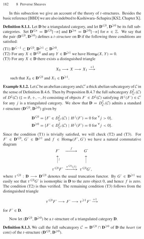
182 8 Perverse Sheaves
In this subsection we give an account of the theory of t-structures. Besides thebasic reference [BBD] we are also indebted to Kashiwara–Schapira [KS2, Chapter X].
Definition 8.1.1. Let D be a triangulated category, and let D�0, D�0 be its full sub-categories. Set D�n = D�0[−n] and D�n = D�0[−n] for n ∈ Z. We say thatthe pair (D�0, D�0) defines a t-structure on D if the following three conditions aresatisfied:
(T1) D�−1 ⊂ D�0, D�1 ⊂ D�0.(T2) For any X ∈ D�0 and any Y ∈ D�1 we have HomD(X, Y ) = 0.(T3) For any X ∈ D there exists a distinguished triangle
X0 −→ X −→ X1+1−→
such that X0 ∈ D�0 and X1 ∈ D�1.
Example 8.1.2. Let C be an abelian category and C′ a thick abelian subcategory of C inthe sense of Definition B.4.6. Then by Proposition B.4.7 the full subcategory D
�
C′(C)
of D�(C) (� = ∅, +, −, b) consisting of objects F · ∈ D�(C) satisfying Hj (F ·) ∈ C′for any j is a triangulated category. We show that D = D
�
C′(C) admits a standardt-structure (D�0, D�0) given by
D�0 = {F˙ ∈ D�
C′(C) | Hj (F˙) = 0 for ∀j > 0},D�0 = {F˙ ∈ D
�
C′(C) | Hj (F˙) = 0 for ∀j < 0}.Since the condition (T1) is trivially satisfied, we will check (T2) and (T3). ForF˙ ∈ D�0, G˙ ∈ D�1 and f ∈ HomD(F˙, G˙) we have a natural commutativediagram
F˙ f−−−−→ G˙�⏐⏐� �⏐⏐τ�0F˙ τ�0(f )−−−−→ τ�0G˙,
where τ�0 : D −→ D�0 denotes the usual truncation functor. By G˙ ∈ D�1 weeasily see that τ�0G˙ is isomorphic in D to the zero object 0, and hence f is zero.The condition (T2) is thus verified. The remaining condition (T3) follows from thedistinguished triangle
τ�0F˙ −→ F˙ −→ τ�1F˙ +1−→for F˙ ∈ D.
Now let (D�0, D�0) be a t-structure of a triangulated category D.
Definition 8.1.3. We call the full subcategory C = D�0 ∩ D�0 of D the heart (orcore) of the t-structure (D�0, D�0).
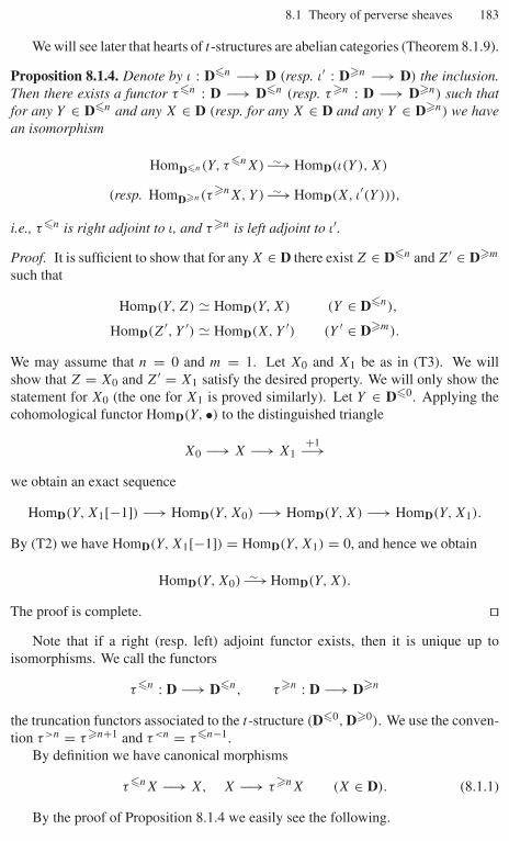
8.1 Theory of perverse sheaves 183
We will see later that hearts of t-structures are abelian categories (Theorem 8.1.9).
Proposition 8.1.4. Denote by ι : D�n −→ D (resp. ι′ : D�n −→ D) the inclusion.Then there exists a functor τ�n : D −→ D�n (resp. τ�n : D −→ D�n) such thatfor any Y ∈ D�n and any X ∈ D (resp. for any X ∈ D and any Y ∈ D�n) we havean isomorphism
HomD�n(Y, τ�nX) −→∼ HomD(ι(Y ), X)
(resp. HomD�n(τ�nX, Y ) −→∼ HomD(X, ι′(Y ))),
i.e., τ�n is right adjoint to ι, and τ�n is left adjoint to ι′.
Proof. It is sufficient to show that for any X ∈ D there exist Z ∈ D�n and Z′ ∈ D�m
such that
HomD(Y, Z) � HomD(Y, X) (Y ∈ D�n),
HomD(Z′, Y ′) � HomD(X, Y ′) (Y ′ ∈ D�m).
We may assume that n = 0 and m = 1. Let X0 and X1 be as in (T3). We willshow that Z = X0 and Z′ = X1 satisfy the desired property. We will only show thestatement for X0 (the one for X1 is proved similarly). Let Y ∈ D�0. Applying thecohomological functor HomD(Y, •) to the distinguished triangle
X0 −→ X −→ X1+1−→
we obtain an exact sequence
HomD(Y, X1[−1]) −→ HomD(Y, X0) −→ HomD(Y, X) −→ HomD(Y, X1).
By (T2) we have HomD(Y, X1[−1]) = HomD(Y, X1) = 0, and hence we obtain
HomD(Y, X0) −→∼ HomD(Y, X).
The proof is complete. ��Note that if a right (resp. left) adjoint functor exists, then it is unique up to
isomorphisms. We call the functors
τ�n : D −→ D�n, τ�n : D −→ D�n
the truncation functors associated to the t-structure (D�0, D�0). We use the conven-tion τ>n = τ�n+1 and τ<n = τ�n−1.
By definition we have canonical morphisms
τ�nX −→ X, X −→ τ�nX (X ∈ D). (8.1.1)
By the proof of Proposition 8.1.4 we easily see the following.

184 8 Perverse Sheaves
Proposition 8.1.5.(i) The canonical morphisms (8.1.1) is embedded into a distinguished triangle
τ�n(X) −→ X −→ τ�n+1(X)+1−→ (8.1.2)
in D.(ii) For X ∈ D let
X0 −→ X −→ X1+1−→
be as in (T3). Then there exist identifications X0 � τ�0X and X1 � τ�1X bywhich the morphisms X0 → X and X → X1 are identified with the canonicalones (8.1.1). In particular, X0 and X1 are uniquely determined from X ∈ D.
Proposition 8.1.6. The following conditions on X ∈ D are equivalent:
(i) We have X ∈ D�n (resp. X ∈ D�n).(ii) The canonical morphism τ�nX → X (resp. X → τ�nX) is an isomorphism.
(iii) We have τ>nX = 0 (resp. τ<nX = 0).
Proof. The equivalence of (ii) and (iii) is obvious in view of (8.1.2). The implication(ii)=⇒(i) is obvious by τ�nX ∈ D�n and τ�nX ∈ D�n. It remains to show(i)=⇒(ii). Let us show that the canonical morphism τ�nX → X is an isomorphismfor X ∈ D�n. We may assume that n = 0. By applying Proposition 8.1.5 (ii) to theobvious distinguished triangle
Xid−→ X −→ 0
+1−→we see that the canonical morphism τ�0X → X is an isomorphism. The remainingassertion is proved similarly. ��Lemma 8.1.7. Let
X′ −→ X −→ X′′ +1−→be a distinguished triangle in D. If X′, X′′ ∈ D�0 (resp. D�0), then X ∈ D�0 (resp.D�0). In particular, if X′, X′′ ∈ C, then X ∈ C.
Proof. We only prove the assertion for D�0. Assume that X′, X′′ ∈ D�0. ByProposition 8.1.6 it is enough to show τ>0(X) = 0. In the exact sequence
HomD(X′′, τ>0(X)) −→ HomD(X, τ>0(X)) −→ HomD(X′, τ>0(X))
we have HomD(X′′, τ>0(X)) = HomD(X′, τ>0(X)) = 0 by (T2), and henceHomD(τ>0(X), τ>0(X)) = HomD(X, τ>0(X)) = 0 by Proposition 8.1.4. Thisimplies τ>0(X) = 0. ��Proposition 8.1.8. Let a, b be two integers.
(i) If b ≥ a, then we have τ�b ◦ τ�a � τ�a ◦ τ�b � τ�a and τ�b ◦ τ�a �τ�a ◦ τ�b � τ�b.
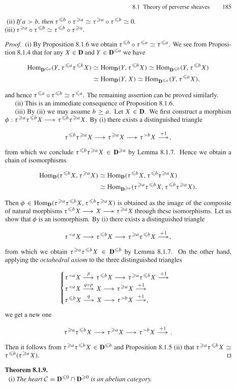
8.1 Theory of perverse sheaves 185
(ii) If a > b, then τ�b ◦ τ�a � τ�a ◦ τ�b � 0.(iii) τ�a ◦ τ�b � τ�b ◦ τ�a .
Proof. (i) By Proposition 8.1.6 we obtain τ�b ◦ τ�a � τ�a . We see from Proposi-tion 8.1.4 that for any X ∈ D and Y ∈ D�a we have
HomD�a (Y, τ�aτ�bX) � HomD(Y, τ�bX) � HomD�b (Y, τ�bX)
� HomD(Y, X) � HomD�a (Y, τ�aX),
and hence τ�a ◦ τ�b � τ�a . The remaining assertion can be proved similarly.(ii) This is an immediate consequence of Proposition 8.1.6.(iii) By (ii) we may assume b ≥ a. Let X ∈ D. We first construct a morphism
φ : τ�aτ�bX −→ τ�bτ�aX. By (i) there exists a distinguished triangle
τ�bτ�aX −→ τ�aX −→ τ>bX+1−→,
from which we conclude τ�bτ�aX ∈ D�a by Lemma 8.1.7. Hence we obtain achain of isomorphisms
HomD(τ�bX, τ�aX) � HomD(τ�bX, τ�bτ�aX)
� HomD�a (τ�aτ�bX, τ�bτ�aX).
Then φ ∈ HomD(τ�aτ�bX, τ�bτ�aX) is obtained as the image of the compositeof natural morphisms τ�bX −→ X −→ τ�aX through these isomorphisms. Let usshow that φ is an isomorphism. By (i) there exists a distinguished triangle
τ<aX −→ τ�bX −→ τ�aτ�bX+1−→,
from which we obtain τ�aτ�bX ∈ D�b by Lemma 8.1.7. On the other hand,applying the octahedral axiom to the three distinguished triangles⎧⎪⎪⎨⎪⎪⎩
τ<aXp−→ τ�bX −→ τ�aτ�bX
+1−→τ<aX
q◦p−→ X −→ τ�aX+1−→
τ�bXq−→ X −→ τ>bX
+1−→,
we get a new one
τ�aτ�bX −→ τ�aX −→ τ>bX+1−→ .
Then it follows from τ�aτ�bX ∈ D�b and Proposition 8.1.5 (ii) that τ�aτ�bX �τ�b(τ�aX). ��Theorem 8.1.9.
(i) The heart C = D�0 ∩ D�0 is an abelian category.
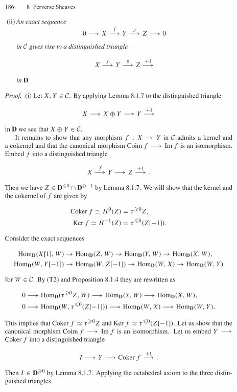
186 8 Perverse Sheaves
(ii) An exact sequence
0 −→ Xf−→ Y
g−→ Z −→ 0
in C gives rise to a distinguished triangle
Xf−→ Y
g−→ Z+1−→
in D.
Proof. (i) Let X, Y ∈ C. By applying Lemma 8.1.7 to the distinguished triangle
X −→ X ⊕ Y −→ Y+1−→
in D we see that X ⊕ Y ∈ C.It remains to show that any morphism f : X → Y in C admits a kernel and
a cokernel and that the canonical morphism Coim f −→ Im f is an isomorphism.Embed f into a distinguished triangle
Xf−→ Y −→ Z
+1−→ .
Then we have Z ∈ D�0 ∩ D�−1 by Lemma 8.1.7. We will show that the kernel andthe cokernel of f are given by
Coker f � H 0(Z) = τ�0Z,
Ker f � H−1(Z) = τ�0(Z[−1]).Consider the exact sequences
HomD(X[1], W) → HomD(Z, W) → HomD(Y, W) → HomD(X, W),
HomD(W, Y [−1]) → HomD(W, Z[−1]) → HomD(W, X) → HomD(W, Y )
for W ∈ C. By (T2) and Proposition 8.1.4 they are rewritten as
0 −→ HomD(τ�0Z, W) −→ HomD(Y, W) −→ HomD(X, W),
0 −→ HomD(W, τ�0(Z[−1])) −→ HomD(W, X) −→ HomD(W, Y ).
This implies that Coker f � τ�0Z and Ker f � τ�0(Z[−1]). Let us show that thecanonical morphism Coim f −→ Im f is an isomorphism. Let us embed Y −→Coker f into a distinguished triangle
I −→ Y −→ Coker f+1−→ .
Then I ∈ D�0 by Lemma 8.1.7. Applying the octahedral axiom to the three distin-guished triangles
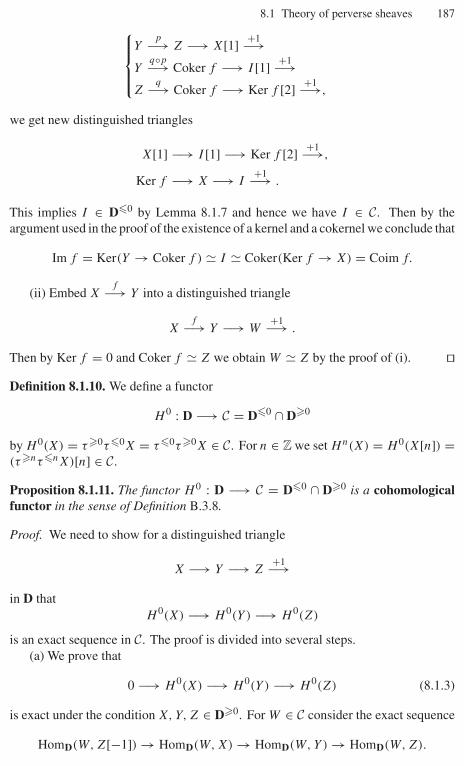
8.1 Theory of perverse sheaves 187⎧⎪⎪⎨⎪⎪⎩Y
p−→ Z −→ X[1] +1−→Y
q◦p−→ Coker f −→ I [1] +1−→Z
q−→ Coker f −→ Ker f [2] +1−→,
we get new distinguished triangles
X[1] −→ I [1] −→ Ker f [2] +1−→,
Ker f −→ X −→ I+1−→ .
This implies I ∈ D�0 by Lemma 8.1.7 and hence we have I ∈ C. Then by theargument used in the proof of the existence of a kernel and a cokernel we conclude that
Im f = Ker(Y → Coker f ) � I � Coker(Ker f → X) = Coim f.
(ii) Embed Xf−→ Y into a distinguished triangle
Xf−→ Y −→ W
+1−→ .
Then by Ker f = 0 and Coker f � Z we obtain W � Z by the proof of (i). ��Definition 8.1.10. We define a functor
H 0 : D −→ C = D�0 ∩ D�0
by H 0(X) = τ�0τ�0X = τ�0τ�0X ∈ C. For n ∈ Z we set Hn(X) = H 0(X[n]) =(τ�nτ�nX)[n] ∈ C.
Proposition 8.1.11. The functor H 0 : D −→ C = D�0 ∩ D�0 is a cohomologicalfunctor in the sense of Definition B.3.8.
Proof. We need to show for a distinguished triangle
X −→ Y −→ Z+1−→
in D thatH 0(X) −→ H 0(Y ) −→ H 0(Z)
is an exact sequence in C. The proof is divided into several steps.(a) We prove that
0 −→ H 0(X) −→ H 0(Y ) −→ H 0(Z) (8.1.3)
is exact under the condition X, Y, Z ∈ D�0. For W ∈ C consider the exact sequence
HomD(W, Z[−1]) → HomD(W, X) → HomD(W, Y ) → HomD(W, Z).

188 8 Perverse Sheaves
By (T2) we have HomD(W, Z[−1]) = 0. Moreover, for V ∈ D�0 we haveτ�0V � τ�0τ�0V = H 0(V ), and hence HomD(W, V ) � HomD(W, τ�0V ) �HomC(W, H 0(V )) by Proposition 8.1.4. Hence the above exact sequence is rewrit-ten as
0 −→ HomC(W, H 0(X)) −→ HomC(W, H 0(Y )) −→ HomC(W, H 0(Z)),
from which we obtain our assertion.(b) We prove that (8.1.3) is exact assuming only Z ∈ D�0. Let W ∈ D<0.
Then we have HomD(W, Z) = HomD(W, Z[−1]) = 0 and hence HomD(W, X) �HomD(W, Y ). By Proposition 8.1.4 this implies that the canonical morphismτ<0X −→ τ<0Y is an isomorphism. Therefore, applying the octahedral axiomto the distinguished triangles⎧⎪⎪⎨⎪⎪⎩
τ<0Xp−→ X −→ τ�0X
+1−→τ<0X
q◦p−→ Y −→ τ�0Y+1−→
Xq−→ Y −→ Z
+1−→,
we get a new one
τ�0X −→ τ�0Y −→ Z+1−→ .
Hence our assertion is a consequence of (a).(c) Similarly to (b) we can prove that
H 0(X) −→ H 0(Y ) −→ H 0(Z) −→ 0
is exact under the condition X ∈ D�0.(d) Finally, let us consider the general case. Embed the composite of the mor-
phisms τ�0X −→ X −→ Y into a distinguished triangle
τ�0X −→ Y −→ W+1−→ .
By applying (c) we have an exact sequence
H 0(X) −→ H 0(Y ) −→ H 0(W).
Now applying the octahedral axiom to the distinguished triangles⎧⎪⎪⎨⎪⎪⎩τ�0X
r−→ X −→ τ>0X+1−→
τ�0Xs◦r−→ Y −→ W
+1−→X
s−→ Y −→ Z+1−→,
we get a distinguished triangle
W −→ Z −→ τ>0X[1] +1−→ .
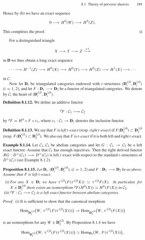
8.1 Theory of perverse sheaves 189
Hence by (b) we have an exact sequence
0 −→ H 0(W) −→ H 0(Z).
This completes the proof. ��For a distinguished triangle
X −→ Y −→ Z+1−→
in D we thus obtain a long exact sequence
· · · −→ H−1(Z) −→ H 0(X) −→ H 0(Y ) −→ H 0(Z) −→ H 1(X) −→ · · ·in C.
Now let Di be triangulated categories endowed with t-structures (D�0i , D�0
i )
(i = 1, 2), and let F : D1 −→ D2 be a functor of triangulated categories. We denoteby Ci the heart of (D�0
i , D�0i ).
Definition 8.1.12. We define an additive functor
pF : C1 −→ C2
by pF = H 0 ◦ F ◦ ε1, where ε1 : C1 → D1 denotes the inclusion functor.
Definition 8.1.13. We say that F is left t-exact (resp. right t-exact) if F(D�01 ) ⊂ D�0
2
(resp. F(D�01 ) ⊂ D�0
2 ). We also say that F is t-exact if it is both left and right t-exact.
Example 8.1.14. Let C1, C2 be abelian categories and let G : C1 → C2 be a leftexact functor. Assume that C1 has enough injectives. Then the right derived functorRG : D+(C1) −→ D+(C2) is left t-exact with respect to the standard t-structures ofD+(Ci ) (see Example 8.1.2).
Proposition 8.1.15. Let Di , (D�0i , D�0
i ), (i = 1, 2) and F : D1 −→ D2 be as above.Assume that F is left t-exact.
(i) For any X ∈ D1 we have τ�0(F (τ�0X)) � τ�0F(X). In particular, forX ∈ D�0
1 there exists an isomorphism pF (H 0(X)) � H 0(F (X)) in C2.(ii) pF : C1 −→ C2 is a left exact functor between abelian categories.
Proof. (i) It is sufficient to show that the canonical morphism
HomD�0
2
(W, τ�0(F (τ�0(X)))
) → HomD�0
2
(W, τ�0(F (X))
)is an isomorphism for any W ∈ D�0
2 . By Proposition 8.1.4 we have
HomD�0
2
(W, τ�0(F (τ�0(X)))
) � HomD2
(W, F(τ�0(X))
),
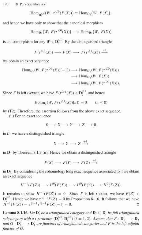
190 8 Perverse Sheaves
HomD�0
2
(W, τ�0(F (X))
) � HomD2
(W, F(X)
),
and hence we have only to show that the canonical morphism
HomD2
(W, F(τ�0(X))
) −→ HomD2
(W, F(X)
)is an isomorphism for any W ∈ D�0
2 . By the distinguished triangle
F(τ�0(X)) −→ F(X) −→ F(τ�1(X))+1−→
we obtain an exact sequence
HomD2(W, F (τ�1(X))[−1]) −→ HomD2(W, F (τ�0(X)))
−→ HomD2(W, F (X))
−→ HomD2(W, F (τ�1(X))).
Since F is left t-exact, we have F(τ�1(X)) ∈ D�12 , and hence
HomD2(W, F (τ�1(X))[n]) = 0 (n ≤ 0)
by (T2). Therefore, the assertion follows from the above exact sequence.(ii) For an exact sequence
0 −→ X −→ Y −→ Z −→ 0
in C1 we have a distinguished triangle
X −→ Y −→ Z+1−→
in D1 by Theorem 8.1.9 (ii). Hence we obtain a distinguished triangle
F(X) −→ F(Y ) −→ F(Z)+1−→
in D2. By considering the cohomology long exact sequence associated to it we obtainan exact sequence
H−1(F (Z)) −→ H 0(F (X)) −→ H 0(F (Y )) −→ H 0(F (Z)).
It remains to show H−1(F (Z)) = 0. Since F is left t-exact, we have F(Z) ∈D�0
2 . Hence we have τ�−1F(Z) = 0 by Proposition 8.1.6. It follows that we haveH−1(F (Z)) = τ�−1τ�−1F(Z)[−1] = 0. ��Lemma 8.1.16. Let D′
i be a triangulated category and Di ⊂ D′i its full triangulated
subcategory with a t-structure (D�0i , D�0
i ) (i = 1, 2). Assume that F : D′1 −→ D′
2and G : D′
2 −→ D′1 are functors of triangulated categories and F is the left adjoint
functor of G.
8.1 Theory of perverse sheaves 191
(i) If F(D1) ⊂ D2 and F(D�01 ) ⊂ D�d
2 for d ∈ Z, then for any Y ∈ D�02 satisfying
G(Y) ∈ D1 we have G(Y) ∈ D�−d1 .
(ii) If G(D2) ⊂ D1 and G(D�02 ) ⊂ D�−d
1 for d ∈ Z, then for any X ∈ D�01 satisfying
F(X) ∈ D2 we have F(X) ∈ D�d2 .
Proof. We prove only the assertion (i). By Proposition 8.1.6 it is enough to showτ<−dG(Y ) = 0. According to Proposition 8.1.4, for any X ∈ D<−d
1 we have anisomorphism
HomD<−d1
(X, τ<−dG(Y )) � HomD1(X, G(Y ))
� HomD2(F (X), Y ) = 0
(note F(X) ∈ D<02 and Y ∈ D�0
2 ). Therefore, we have τ<−dG(Y ) = 0. ��Corollary 8.1.17. Let Di be a triangulated category with a t-structure (i = 1, 2).Assume that F : D1 −→ D2 and G : D2 −→ D1 are functors of triangulatedcategories and F is the left adjoint functor of G. Then F is right t-exact if and onlyif G is left t-exact.
8.1.2 Perverse sheaves
From now on, let X be a (not necessarily smooth) algebraic variety or an analytic spaceand denote by Db
c (X) the full subcategory of Db(X) = Db(Mod(CX)) consisting ofobjects F · ∈ Db(X) such that Hj (F ·) is a constructible sheaf on X for any j . For thedefinition of constructible sheaves and basic properties of Db
c (X) see Section 4.5. The
aim of this subsection is to introduce the perverse t-structure (pD�0c (X), pD
�0c (X))
on D = Dbc (X) and define the category of perverse sheaves on X to be its heart
pD�0c (X) ∩ pD
�0c (X). We follow the basic reference [BBD]. We are also indebted
to [GM1], [G1], and [KS2, Chapter X].
Remark 8.1.18.(i) Although we restrict ourselves to the case of complex coefficients, all of the
results that we present in Sections 8.1.2 and 8.2 remain valid even after replacingMod(CX) with Mod(QX). In particular, we have the notion perverse sheavesand intersection cohomology groups with coefficients in Q. They are essentialfor the theory of Hodge modules to be explained in Section 8.3.
(ii) The t-structure that we treat here is the one with respect to the “middle perversity’’in the terminology of [GM1].
(iii) There exists a more general theory of perverse sheaves on subanalytic spaces asexplained in [KS2, Chapter X].
Notation 8.1.19. For a locally closed analytic subspace S of X we denote its dimen-sion by dS . The inclusion map S ↪−→ X is usually denoted by iS .
Recall that we denote by DX : Dbc (X)op −→∼ Db
c (X) the Verdier duality functor.
192 8 Perverse Sheaves
Definition 8.1.20. We define full subcategories pD�0c (X) and pD
�0c (X) of Db
c (X) as
follows. For F˙ ∈ Dbc (X) we have F˙ ∈ pD
�0c (X) if and only if
(i) dim{supp Hj (F˙)} ≤ −j for any j ∈ Z,
and F˙ ∈ pD�0c (X) if and only if
(ii) dim{supp Hj (DXF˙)} ≤ −j for any j ∈ Z,
We define a full subcategory Perv(CX) of Dbc (X) by
Perv(CX) = pD�0c (X) ∩ pD�0
c (X).
We will show later that the pair (pD�0c (X), pD
�0c (X)) defines a t-structure on
Dbc (X), and hence Perv(CX) will turn out to be an abelian category. Since we have
DXDXF˙ � F˙ for any F˙ ∈ Dbc (X), the Verdier duality functor DX(•) exchanges
pD�0c (X) with pD
�0c (X).
Lemma 8.1.21. Let F˙ ∈ Dbc (X). Then we have
supp Hj (DXF˙) = {x ∈ X| H−j (i!{x}F˙) = 0}for any j ∈ Z, where i{x} : {x} ↪−→ X are inclusion maps.
Proof. Since for each x ∈ X we have
i!{x}F˙ � i!{x}DXDXF˙ � D{x}i−1{x}(DXF˙),
we obtain an isomorphism H−j (i!{x}F˙) � [Hj (DXF˙)x]∗ for any j ∈ Z. ��Proposition 8.1.22. Let F˙ ∈ Db
c (X) and X = ⊔α∈A Xα be a complex stratification
of X consisting of connected strata such that i−1Xα
F˙ and i!XαF˙ have locally constant
cohomology sheaves for any α ∈ A. Then
(i) F˙ ∈ pD�0c (X) if and only if Hj (i−1
XαF˙) = 0 for any α and j > −dXα .
(ii) F˙ ∈ pD�0c (X) if and only if Hj (i!Xα
F˙) = 0 for any α and j < −dXα .
Proof. (i) Trivial.(ii) By Lemma 8.1.21, F˙ ∈ pD
�0c (X) if and only if
dim{x ∈ X| H−j (i!{x}F˙) = 0} ≤ −j
for any j ∈ Z. For x ∈ Xα decompose the morphism i{x} : {x} ↪−→ X into
{x} j{x}↪−→ Xα
iXα↪−→ X. Then we have an isomorphism
i!{x}F˙ � j !{x}i!XαF˙ � j−1
{x} i!Xα
F˙[−2dXα ], (8.1.4)
where we used our assumption on i!XαF˙ in the last isomorphism. Hence for any
j ∈ Z by the connectedness of Xα , Xα ∩ {x ∈ X| H−j (i!{x}F˙) = 0} = Xα ∩supp Hj (DXF˙) is Xα or ∅. Moreover, from (8.1.4) we easily see that the followingconditions are equivalent for any α ∈ A:
8.1 Theory of perverse sheaves 193
(a) Hj (i!XαF˙) = 0 for any j < −dXα .
(b) H−j (i!{x}F˙) = 0 for any x ∈ Xα and j > −dXα .
(c) Xα ∩ supp Hj (DXF˙) = ∅ for any j > −dXα .
The last condition (c) implies that for any stratum Xα such that Xα ⊂ supp Hj (DXF˙)we must have dXα ≤ −j . This completes the proof. ��Corollary 8.1.23. Assume that X is a connected complex manifold and all the coho-mology sheaves of F˙ ∈ Db
c (X) are locally constant on X. Then
(i) F˙ ∈ pD�0c (X) if and only if Hj (F˙) = 0 for any j > −dX.
(ii) F˙ ∈ pD�0c (X) if and only if Hj (F˙) = 0 for any j < −dX.
Proposition 8.1.24. Let F˙ ∈ Dbc (X). Then the following four conditions are equiv-
alent:
(i) F˙ ∈ pD�0c (X).
(ii) For any locally closed analytic subset S of X we have
Hj (i!S(F˙)) = 0 for any j < −dS.
(iii) For any locally closed analytic subset S of X we have
HjS (F˙) = Hj R�S(F˙) = 0 for any j < −dS.
(iv) For any locally closed “smooth’’ analytic subset S of X we have
Hj (i!S(F˙)) = 0 for any j < −dS.
Proof. First, since we have HiS(•) = HiRiS∗i!S(•), the conditions (ii) and (iii) are
equivalent. Let us prove the equivalence of (ii) and (iv). Assume that the condition(iv) is satisfied for F˙ ∈ Db
c (X). We will show that
Hj (i!Z(F˙)) = 0 for any j < −dZ. (8.1.5)
for any locally closed (possibly singular) analytic subset Z of X by induction ondim Z. Denote by Zreg the smooth part of Z and set Z′ = Z \ Zreg. Then dim Z′ <
dim Z and our hypothesis of induction implies that
Hj
Z′(F˙) = 0 for any j < −dZ′ .
In particular, we have
Hj
Z′(F˙) = 0 for any j < −dZ.
So the assertion (8.1.5) follows from (iv) and the distinguished triangle
R�Z′(F˙) −→ R�Z(F˙) −→ R�Zreg(F˙) +1−→ .

194 8 Perverse Sheaves
Now let us take a complex stratification X = �α∈AXα of X consisting of con-nected strata such that i−1
XαF˙ and i!Xα
F˙ have locally constant cohomology sheavesfor any α ∈ A. Then by Proposition 8.1.22 the condition (i) is equivalent to the oneHj (i!Xα
F˙) = 0 for any α and j < −dXα . Therefore, if we take S = Xα in (iv)we see that (iv) implies (i). It remains to prove that (i) implies (iv). Assume thatHj (i!Xα
F˙) = 0 for any α and j < −dXα . For any locally closed (smooth) analyticsubset S in X, we need to show that
Hj (i!S(F˙)) = 0 for any j < −dS.
Set Xk = ⊔dim Xα≤k Xα in X (k = −1, 0, 1, . . . , dX). Since
X−1 = ∅ ⊂ X0 ⊂ · · · ⊂ XdX= X,
it is enough to prove the following assertions (P)k by induction on k:
(P)k : HjS∩Xk
(F˙) = 0 for any j < −dS. (8.1.6)
Moreover, by the distinguished triangles
R�S∩Xk−1(F˙) −→ R�S∩Xk(F˙) −→ R�S∩(Xk\Xk−1)(F˙) +1−→
for k = 0, 1, . . . , dX, we can reduce the problem to the proof of the assertions
(Q)k : Hj
S∩(Xk\Xk−1)(F˙) = 0 for any j < −dS. (8.1.7)
Note that Xk \ Xk−1 is the union of k-dimensional strata. Hence we obtain a directsum decomposition
Hj
S∩(Xk\Xk−1)(F˙) �⊕
dim Xα=k
HjS∩Xα
(F˙)
and it remains to show Hj (i!S∩XαF˙) � 0 for any α ∈ A and j < −dS . Decomposing
iS∩Xα : S ∩ Xα ↪−→ X into S ∩ Xα
jXα↪−→ Xα
iXα↪−→ X we obtain an isomorphism
i!S∩XαF˙ � j !
Xα(i!Xα
(F˙)). Therefore, by applying Lemma 8.1.25 below to Y = Xα
and G˙ = i!Xα(F˙) ∈ Db
c (Y ) we obtain
Hj j !Xα
(G˙) � Hj i!S∩Xα(F˙) � 0 for any j < −dS∩Xα .
This completes the proof. ��Lemma 8.1.25. Let Y be a complex manifold and G˙ ∈ Db
c (Y ). Assume that all thecohomology sheaves of G˙are locally constant on Y and for an integer d ∈ Z we haveHj G˙ = 0 for j < d. Then for any locally closed analytic subset Z of Y we have
HjZ(G˙) = 0 for any j < d + 2 codimY Z.
8.1 Theory of perverse sheaves 195
Proof. By induction on the cohomological length of G˙ we may assume that G˙ is alocal system L on Y . Since the question is local on Y , we may further assume that L
is the constant sheaf CY . Hence it is sufficient to show
HjZ(CY ) = 0 for any j < 2 codimY Z.
This well-known result can be proved by induction on the dimension of Z with thehelp of the distinguished triangle
R�Z\Zreg(CY ) −→ R�Z(CY ) −→ R�Zreg(CY )+1−→ . ��
It is easily seen that F · ∈ Dbc (X) belongs to pD
�0c (X) if and only if the condition
(i)∗ for any Zariski locally closed irreducible subvariety S of X there exists a Zariskiopen dense smooth subset S0 of S such that Hj (i−1
S0F ·) is a local system for any
j and Hj (i−1S0
F ·) = 0 for any j > −dS
is satisfied (see the proof of Lemma 7.2.9). Also by the proof of Proposition 8.1.24,we easily see that F · ∈ Db
c (X) belongs to pD�0c (X) if and only if the condition
(ii)∗ for any Zariski locally closed irreducible subvariety S of X there exists a Zariskiopen dense smooth subset S0 of S such that Hj (i!S0
F ·) is a local system for any
j and Hj (i!S0F ·) = 0 for any j < −dS
is satisfied.
Proposition 8.1.26. Let F˙ ∈ pD�0c (X) and G˙ ∈ pD
�0c (X).
(i) We haveHj (RHomCX
(F˙, G˙)) = 0
for any j < 0.(ii) The correspondence
{open subsets of X} U �−→ HomDb(U)(F˙|U , G˙|U )
defines a sheaf on X.
Proof. (i) Set S = ⋃j<0 supp(Hj (RHomCX
(F˙, G˙))) ⊂ X. Assume that S = ∅.Let iS : S → X be the embedding. For j < 0 we have
supp(Hj RHomCX(F˙, G˙)) ⊂ S,
and hence
Hj RHomCX(F˙, G˙) � Hj (R�SRHomCX
(F˙, G˙))� Hj (iS∗i!SRHomCX
(F˙, G˙))� iS∗Hj (RHomCS
(i−1S F˙, i!SG˙)).
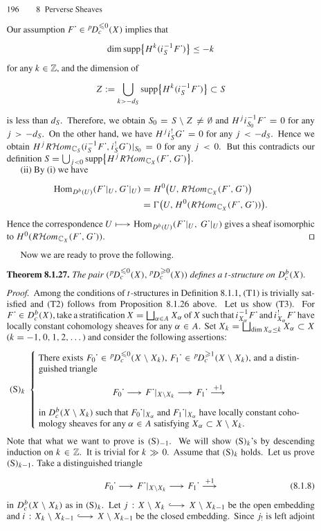
196 8 Perverse Sheaves
Our assumption F˙ ∈ pD�0c (X) implies that
dim supp{Hk(i−1
S F˙)} ≤ −k
for any k ∈ Z, and the dimension of
Z :=⋃
k>−dS
supp{Hk(i−1
S F˙)} ⊂ S
is less than dS . Therefore, we obtain S0 = S \ Z = ∅ and Hj i−1S0
F˙ = 0 for any
j > −dS . On the other hand, we have Hj i!SG˙ = 0 for any j < −dS . Hence weobtain Hj RHomCS
(i−1S F˙, i!SG˙)|S0 = 0 for any j < 0. But this contradicts our
definition S = ⋃j<0 supp
{Hj RHomCX
(F˙, G˙)}.(ii) By (i) we have
HomDb(U)(F˙|U , G˙|U ) = H 0(U, RHomCX(F˙, G˙))
= �(U, H 0(RHomCX
(F˙, G˙))).Hence the correspondence U �−→ HomDb(U)(F˙|U , G˙|U ) gives a sheaf isomorphicto H 0(RHomCX
(F˙, G˙)). ��Now we are ready to prove the following.
Theorem 8.1.27. The pair (pD�0c (X), pD
�0c (X)) defines a t-structure on Db
c (X).
Proof. Among the conditions of t-structures in Definition 8.1.1, (T1) is trivially sat-isfied and (T2) follows from Proposition 8.1.26 above. Let us show (T3). ForF˙ ∈ Db
c (X), take a stratification X = ⊔α∈A Xα of X such that i−1
XαF˙and i!Xα
F˙havelocally constant cohomology sheaves for any α ∈ A. Set Xk = ⊔
dim Xα≤k Xα ⊂ X
(k = −1, 0, 1, 2, . . . ) and consider the following assertions:
(S)k
⎧⎪⎪⎪⎪⎪⎪⎪⎪⎨⎪⎪⎪⎪⎪⎪⎪⎪⎩
There exists F0˙ ∈ pD�0c (X \ Xk), F1˙ ∈ pD
�1c (X \ Xk), and a distin-
guished triangle
F0˙ −→ F˙|X\Xk−→ F1˙ +1−→
in Dbc (X \ Xk) such that F0˙|Xα and F1˙|Xα have locally constant coho-
mology sheaves for any α ∈ A satisfying Xα ⊂ X \ Xk .
Note that what we want to prove is (S)−1. We will show (S)k’s by descendinginduction on k ∈ Z. It is trivial for k � 0. Assume that (S)k holds. Let us prove(S)k−1. Take a distinguished triangle
F0˙ −→ F˙|X\Xk−→ F1˙ +1−→ (8.1.8)
in Dbc (X \ Xk) as in (S)k . Let j : X \ Xk ↪−→ X \ Xk−1 be the open embedding
and i : Xk \ Xk−1 ↪−→ X \ Xk−1 be the closed embedding. Since j! is left adjoint

8.1 Theory of perverse sheaves 197
to j !, the morphism F0˙ −→ j !(F˙|X\Xk−1) � F˙|X\Xkgives rise to a morphism
j!F0˙ −→ F˙|X\Xk−1 . Let us embed this morphism into a distinguished triangle
j!F0˙ −→ F˙|X\Xk−1 −→ G˙ +1−→ . (8.1.9)
We also embed the composite of the morphisms τ�−ki!i!G˙ −→ i!i!G˙ −→ G˙ intoa distinguished triangle
τ�−ki!i!G˙ −→ G˙ −→ F1˙ +1−→ . (8.1.10)
We finally embed the composite of F˙|X\Xk−1 −→ G˙ −→ F1˙ into a distinguishedtriangle
F0˙ −→ F˙|X\Xk−1 −→ F1˙ +1−→ . (8.1.11)
By our construction F0˙|Xα and F1˙|Xα have locally constant cohomology sheaves for
any α ∈ A satisfying Xα ⊂ X \ Xk−1. It remains to show F0˙ ∈ pD�0c (X \ Xk−1)
and F1˙ ∈ pD�1c (X \ Xk−1). Applying the functor j−1(•) to (8.1.10) and (8.1.9), we
get an isomorphism j−1F1˙ � j−1G˙ and a distinguished triangle
F0˙ −→ F˙|X\Xk−→ j−1F1˙ +1−→ .
Hence we have j−1F1˙ � F1 , and j−1F0˙ � F0˙ by (8.1.8) and (8.1.11). Therefore,we have only to show that
(i) Hj (i−1F0˙) = 0 for ∀j > −k
(ii) Hj (i!F1˙) = 0 for ∀j < −k + 1
in view of Proposition 8.1.22 (note that Xk \Xk−1 is a union of k-dimensional strata).By applying the octahedral axiom to the three distinguished triangles⎧⎪⎪⎨⎪⎪⎩
j!F0˙ −→ F˙|X\Xk−1
f−→ G˙ +1−→F0˙ −→ F˙|X\Xk−1
g◦f−−→ F1˙ +1−→τ�−ki!i!G˙ −→ G˙ g−→ F1˙ +1−→
we obtain a distinguished triangle
j!F0˙ −→ F0˙ −→ τ�−ki!i!G˙ +1−→ .
Hence we have i−1F0˙ � i−1τ�−ki!i!G˙ � i−1i!τ�−ki!G˙ � τ�−ki!G . The asser-tion (i) is proved. By applying the functor i! to (8.1.10) we obtain a distinguishedtriangle
i!τ�−ki!i!G˙ −→ i!G˙ −→ i!F1˙ +1−→ .
We have i!τ�−ki!i!G � i!i!τ�−ki!G � τ�−ki!G, and hence we obtain i!F1˙ �τ�−k+1(i!G˙) by this distinguished triangle. The assertion (ii) is also proved. ��
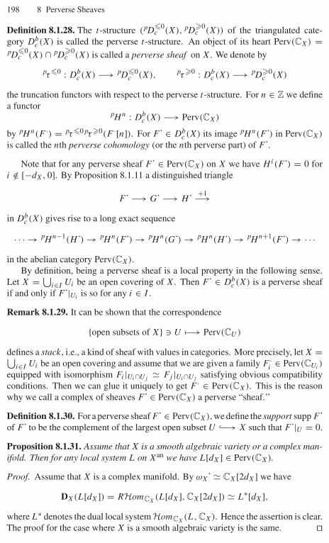
198 8 Perverse Sheaves
Definition 8.1.28. The t-structure (pD�0c (X), pD
�0c (X)) of the triangulated cate-
gory Dbc (X) is called the perverse t-structure. An object of its heart Perv(CX) =
pD�0c (X) ∩ pD
�0c (X) is called a perverse sheaf on X. We denote by
pτ�0 : Dbc (X) −→ pD�0
c (X), pτ�0 : Dbc (X) −→ pD�0
c (X)
the truncation functors with respect to the perverse t-structure. For n ∈ Z we definea functor
pHn : Dbc (X) −→ Perv(CX)
by pHn(F ·) = pτ�0pτ�0(F ·[n]). For F˙ ∈ Dbc (X) its image pHn(F˙) in Perv(CX)
is called the nth perverse cohomology (or the nth perverse part) of F .
Note that for any perverse sheaf F˙ ∈ Perv(CX) on X we have Hi(F˙) = 0 fori /∈ [−dX, 0]. By Proposition 8.1.11 a distinguished triangle
F˙ −→ G˙ −→ H˙ +1−→in Db
c (X) gives rise to a long exact sequence
· · · → pHn−1(H˙) → pHn(F˙) → pHn(G˙) → pHn(H˙) → pHn+1(F˙) → · · ·in the abelian category Perv(CX).
By definition, being a perverse sheaf is a local property in the following sense.Let X = ⋃
i∈I Ui be an open covering of X. Then F˙ ∈ Dbc (X) is a perverse sheaf
if and only if F˙|Uiis so for any i ∈ I .
Remark 8.1.29. It can be shown that the correspondence
{open subsets of X} U �−→ Perv(CU )
defines a stack, i.e., a kind of sheaf with values in categories. More precisely, let X =⋃i∈I Ui be an open covering and assume that we are given a family F ·
i ∈ Perv(CUi)
equipped with isomorphism Fi |Ui∩Uj� Fj |Ui∩Uj
satisfying obvious compatibilityconditions. Then we can glue it uniquely to get F · ∈ Perv(CX). This is the reasonwhy we call a complex of sheaves F˙ ∈ Perv(CX) a perverse “sheaf.’’
Definition 8.1.30. For a perverse sheaf F˙ ∈ Perv(CX), we define the support supp F˙of F˙ to be the complement of the largest open subset U ↪−→ X such that F˙|U = 0.
Proposition 8.1.31. Assume that X is a smooth algebraic variety or a complex man-ifold. Then for any local system L on Xan we have L[dX] ∈ Perv(CX).
Proof. Assume that X is a complex manifold. By ωX˙ � CX[2dX] we have
DX(L[dX]) = RHomCX(L[dX], CX[2dX]) � L∗[dX],
where L∗ denotes the dual local system HomCX(L, CX). Hence the assertion is clear.
The proof for the case where X is a smooth algebraic variety is the same. ��

8.1 Theory of perverse sheaves 199
Remark 8.1.32. More generally, it is known that if X is a pure-dimensional alge-braic variety (resp. analytic space) which is locally a complete intersection, thenwe have L[dX] ∈ Perv(CX) for any local system L on Xan (see for instance [Di,Theorem 5.1.20]).
The following proposition is obvious in view of the definition of pD�0c (X) and
pD�0c (X).
Proposition 8.1.33. The Verdier duality functor DX : Dbc (X) → Db
c (X)op is t-exactand induces an exact functor
DX : Perv(CX) −→ Perv(CX)op.
Proposition 8.1.34. Let i : Z ↪−→ X be an embedding of a closed subvariety Z ofX. Then the functor i∗ sends Perv(CZ) to Perv(CX).
Proof. It is easily seen that i∗ sends pD�0c (Z) to pD
�0c (X). Since Z is closed, we
have i∗ = i! = DX ◦ i∗ ◦ DZ . Hence i∗ sends pD�0c (Z) to pD
�0c (X). ��
By Propositions 8.1.31 and 8.1.34 we obtain the following.
Example 8.1.35.(i) Let X be a (possibly singular) analytic space and Y ⊂ X a smooth complex
manifold contained in X as a closed subset. Then for any local system L on Y ,the complex iY ∗(L[dY ]) ∈ Db
c (X) is a perverse sheaf on X.
(ii) Let X = C and U = C \ {0} j↪−→ X. Then for any local system L on U ,
Rj∗(L[1]), Rj !(L[1]) = j!(L[1]) ∈ Dbc (X) (j! is an exact functor) are perverse
sheaves on X = C.
Definition 8.1.36. Let X, Y be algebraic varieties (or analytic spaces). For a func-tor F : Db
c (X) −→ Dbc (Y ) of triangulated categories we define a functor pF :
Perv(CX) −→ Perv(CY ) to be the composite of the functors
Perv(CX) ↪−→ Dbc (X)
F−→ Dbc (Y )
pH 0−→ Perv(CY ).
Let f : X −→ Y be a morphism of algebraic varieties or analytic spaces. Thenwe have functors
pf −1, pf ! : Perv(CY ) −→ Perv(CX).
Assume that f : X −→ Y is a proper morphism. Then we also have functors
pRf∗, pRf! : Perv(CX) −→ Perv(CY ).
Notation 8.1.37. We sometimes denote the functors pRf ∗, pRf ! by pf∗, pf!, respec-tively, to simplify our notation.
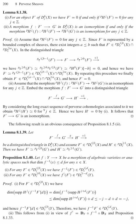
200 8 Perverse Sheaves
Lemma 8.1.38.(i) For an object F˙ of Db
c (X) we have F˙ = 0 if and only if pHj (F˙) = 0 for anyj ∈ Z.
(ii) A morphism f : F˙ −→ G˙ in Dbc (X) is an isomorphism if and only if the
morphism pHj (f ) : pHj (F˙) → pHj (G˙) is an isomorphism for any j ∈ Z.
Proof. (i) Assume that pHj (F˙) = 0 for any j ∈ Z. Since F˙ is represented by abounded complex of sheaves, there exist integers a ≤ b such that F˙ ∈ pD
�bc (X) ∩
pD�ac (X). In the distinguished triangle
pτ�b−1(F˙) −→ F˙ −→ pτ�b(F˙) +1−→we have pτ�b(F˙) � pτ�bpτ�b(F˙) � pHb(F ·)[−b] = 0, and hence we haveF · � pτ�b−1(F˙) ∈ pD
�b−1c (X)∩pD
�ac (X). By repeating this procedure we finally
obtain F · ∈ pD�a−1c (X) ∩ pD
�ac (X), and hence F · = 0.
(ii)Assume that the morphism pHj (f ) : pHj (F˙) → pHj (G˙) is an isomorphismfor any j ∈ Z. Embed the morphism f : F˙ −→ G˙ into a distinguished triangle
F˙ f−→ G˙ −→ H˙ +1−→ .
By considering the long exact sequence of perverse cohomologies associated to it weobtain pHj (H˙) � 0 for ∀j ∈ Z. Hence we have H · = 0 by (i). It follows thatF˙ −→ G˙ is an isomorphism. ��
The following result is an obvious consequence of Proposition 8.1.5 (ii).
Lemma 8.1.39. Let
F˙ f−→ G˙ g−→ H˙ +1−→be a distinguished triangle in Db
c (X) and assume F˙ ∈ pD�0c (X) and H˙ ∈ pD
�1c (X).
Then we have F˙ � pτ�0(G˙) and H˙ � pτ�1(G˙).Proposition 8.1.40. Let f : Y −→ X be a morphism of algebraic varieties or ana-lytic spaces such that dim f −1(x) ≤ d for any x ∈ X.
(i) For any F˙ ∈ pD�0c (X) we have f −1(F˙) ∈ pD
�dc (Y ).
(ii) For any F˙ ∈ pD�0c (X) we have f !(F˙) ∈ pD
�−dc (Y ).
Proof. (i) For F˙ ∈ pD�0c (X) we have
dim(supp Hj (f −1F˙[d])) = dim
(f −1(supp Hj+d(F˙)))
≤ dim(supp Hj+d(F˙))+ d ≤ −j − d + d = −j,
and hence f −1F˙[d] ∈ pD�0c (Y ), Therefore, we have f −1F˙ ∈ pD
�dc (Y ).
(ii) This follows from (i) in view of f ! = DY ◦ f −1 ◦ DX and Proposition8.1.33. ��

8.1 Theory of perverse sheaves 201
Corollary 8.1.41. Let Z be a locally closed subvariety of X and let i : Z → X bethe embedding.
(i) The functor i−1 : Dbc (X) −→ Db
c (Z) is right t-exact with respect to the perverset-structures.
(ii) The functor i! : Dbc (X) −→ Db
c (Z) is left t-exact with respect to the perverset-structures.
The following propositions are immediate consequences of Proposition 8.1.40and Corollary 8.1.41 in view of Lemma 8.1.16.
Proposition 8.1.42. Let f : X → Y be as in Proposition 8.1.40.
(i) For any G˙ ∈ pD�0c (Y ) such that Rf ∗(G˙) ∈ Db
c (X) we have Rf ∗(G˙) ∈pD
�−dc (X).
(ii) For any G˙ ∈ pD�0c (Y ) such that Rf !(G˙) ∈ Db
c (X) we have Rf !(G˙) ∈pD
�dc (X).
Proposition 8.1.43. Let i : Z → X be as in Corollary 8.1.41.
(i) For any G˙ ∈ pD�0c (Z) such that Ri∗(G˙) ∈ Db
c (X) we have Ri∗(G˙) ∈pD
�0c (X).
(ii) For any G˙ ∈ pD�0c (Z) such that i!(G˙) ∈ Db
c (X) we have i!(G˙) ∈ pD�0c (X).
Corollary 8.1.44.
(i) Let j : U ↪−→ X be an inclusion of an open subset U of X. Then j−1 = j ! ist-exact with respect to the perverse t-structures and induces an exact functor
pj−1 = pj ! : Perv(CX) −→ Perv(CU ).
(ii) Let i : Z ↪−→ X be an inclusion of a closed subvariety Z. Then i∗ = i! is t-exactwith respect to the perverse t-structures and induces an exact functor
pi∗ = pi! : Perv(CZ) −→ Perv(CX).
Moreover, if we denote by PervZ(CX) the category of perverse sheaves on X
whose supports are contained in Z, then the functor pi−1 = pi! : PervZ(CX) −→Perv(CZ) is well defined and induces an equivalence
PervZ(CX)
pi−1=pi!
pi∗=pi!−−−−→←−−−− Perv(CZ)
of categories. The functor pi−1 is the quasi-inverse of pi∗.
Lemma 8.1.45. For an exact sequence 0 −→ F˙ −→ G˙ −→ H˙ −→ 0 of perversesheaves on X, we have supp G˙ = supp F˙ ∪ supp H .

202 8 Perverse Sheaves
Proof. We first show supp F˙ ⊂ supp G . Set U = X \ supp G . It is enough to showF˙|U = 0. By Corollary 8.1.44 (i) we have an exact sequence
0 −→ F˙|U φ−→ G˙|Uin the abelian category Perv(CU ). Hence we obtain F˙|U = 0 from G˙|U = 0.The inclusion supp H˙ ⊂ supp G˙ can be proved similarly. Let us show supp G˙ ⊂supp F˙ ∪ supp H . It is sufficient to show that if we have F ·|U = H ·|U = 0 for anopen subset U of X, then G·|U = 0. This follows easily from Theorem 8.1.9 (ii). ��Remark 8.1.46. The formal properties of perverse sheaves on X that we listed abovecarry rich information on the singularities of the base space X. Indeed, using perversesheaves, we can easily recover and even extend various classical results in singularitytheory. For example, see [Di], [Mas1], [Mas2], [NT], [Schu], [Tk2]. Note alsothat Kashiwara [Kas19] recently introduced an interesting t-structure on the categoryDb
rh(DX) whose heart corresponds to the category of constructible sheaves on X
(here X is a smooth algebraic variety) through the Riemann–Hilbert correspondence.
8.2 Intersection cohomology theory
8.2.1 Introduction
Let X be an irreducible projective algebraic variety (or an irreducible compact analyticspace) of dimension dX. If X is non-singular, then we have the Poincaré dualityHi(X, CX) � [
H 2dX−i (X, CX)]∗ for any 0 ≤ i ≤ 2dX. However, for a general
(singular) variety X, we cannot expect such a nice symmetry in its usual cohomologygroups. The intersection cohomology theory of Goresky–MacPherson [GM1] is anew theory which enables us to overcome this problem. The basic idea in theirtheory is to replace the constant sheaf CX with a new complex ICX˙[−dX] ∈ Db
c (X)
of sheaves on X and introduce the intersection cohomology groups
IH i(X) = Hi(X, ICX˙[−dX]) (0 ≤ i ≤ 2dX)
by taking the hypercohomology groups of ICX . Then we obtain a generalizedPoincaré duality
IH i(X) = [IH 2dX−i (X)
]∗(0 ≤ i ≤ 2dX)
for any projective variety X. Moreover, it turns out that intersection cohomologygroups admit the Hodge decomposition. Indeed, Morihiko Saito constructed histheory of Hodge modules to obtain this remarkable generalization of the Hodge–Kodaira theory to singular varieties (see Section 8.3). To define the intersectioncohomology complex ICX˙ ∈ Db
c (X) of X, first we take a constant perverse sheafCU [dX] on a Zariski open dense subset U of the smooth part Xreg of X. Then ICX˙ is a“minimal’’ extension of CU [dX] ∈ Perv(CU ) to a perverse sheaf on the whole X. Let
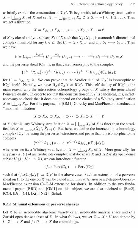
8.2 Intersection cohomology theory 203
us briefly explain the construction of ICX . To begin with, take a Whitney stratificationX = ⊔
α∈A Xα of X and set Xk = ⊔dim Xα≤k Xα ⊂ X (k = −1, 0, 1, 2, . . . ). Then
we get a filtration
X = XdX⊃ XdX−1 ⊃ · · · ⊃ X0 ⊃ X−1 = ∅
of X by closed analytic subsets Xk of X such that Xk\Xk−1 is a smooth k-dimensionalcomplex manifold for any k ∈ Z. Set Uk = X \ Xk−1 and jk : Uk ↪−→ Uk−1. Thenwe have
∅ = UdX+1 ↪jdX+1−−−→ UdX
jdX↪−→ UdX−1 ↪−→ · · · j2
↪−→ U1j1
↪−→ U0 = X
and the perverse sheaf ICX˙ is, in this case, isomorphic to the complex(τ�−1Rj1∗
) ◦ (τ�−2Rj2∗) ◦ · · · ◦ (τ�−dXRjdX ∗
)(CU [dX])
for U = UdX⊂ X. We can prove that the Verdier dual of ICX˙ is isomorphic to
ICX˙ itself. Namely, we have DX(ICX˙) � ICX . This self-duality of ICX˙ is themain reason why the intersection cohomology groups of X satisfy the generalizedPoincaré duality. In order to see that this construction of ICX˙ is canonical, it is, in fact,necessary to check that it does not depend on the choice of a Whitney stratificationX = ⊔
α∈A Xα . For this purpose, in [GM1] Goresky and MacPherson introduced a“maximal’’ filtration
X ⊃ XdX⊃ XdX−1 ⊃ · · · ⊃ X0 ⊃ X−1 = ∅
of X (that is, any Whitney stratification X = ⊔α∈A Xα of X is finer than the strati-
fication X = ⊔k∈Z(Xk \ Xk−1)). But here, we define the intersection cohomology
complex ICX˙ by using the perverse t-structures and prove that it is isomorphic to thecomplex (
τ�−1Rj1∗) ◦ · · · ◦ (τ�−dXRjdX ∗
)(CU [dX])
whenever we fix a Whitney stratification X = ⊔α∈A Xα of X. More generally, for
any pair (X, U) of an irreducible complex analytic space X and its Zariski open densesubset U (j : U ↪−→ X), we can introduce a functor
pj!∗ : Perv(CU ) −→ Perv(CX)
such that pj!∗(CU [dX]) � ICX˙ in the above case. Such an extension of a perversesheaf on U to the one on X will be called a minimal extension or a Deligne–Goresky–MacPherson extension (D-G-M extension for short). In addition to the two funda-mental papers [BBD] and [GM1] on this subject, we are also indebted to [Bor2],[CG], [Di], [G1], [Ki], [Na2], [Schu].
8.2.2 Minimal extensions of perverse sheaves
Let X be an irreducible algebraic variety or an irreducible analytic space and U aZariski open dense subset of X. In what follows, we set Z = X \ U and denote byi : Z ↪−→ X and j : U ↪−→ X the embeddings.
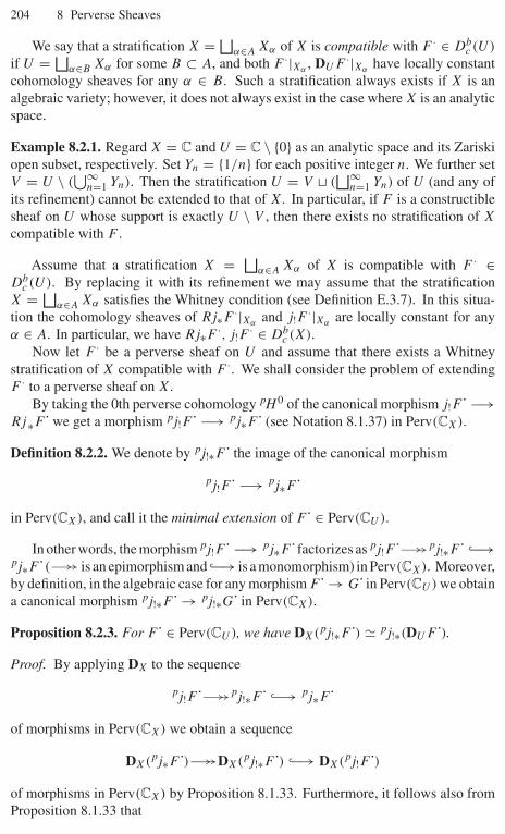
204 8 Perverse Sheaves
We say that a stratification X = ⊔α∈A Xα of X is compatible with F · ∈ Db
c (U)
if U = ⊔α∈B Xα for some B ⊂ A, and both F ·|Xα , DU F ·|Xα have locally constant
cohomology sheaves for any α ∈ B. Such a stratification always exists if X is analgebraic variety; however, it does not always exist in the case where X is an analyticspace.
Example 8.2.1. Regard X = C and U = C \ {0} as an analytic space and its Zariskiopen subset, respectively. Set Yn = {1/n} for each positive integer n. We further setV = U \ (
⋃∞n=1 Yn). Then the stratification U = V � (
⊔∞n=1 Yn) of U (and any of
its refinement) cannot be extended to that of X. In particular, if F is a constructiblesheaf on U whose support is exactly U \ V , then there exists no stratification of X
compatible with F .
Assume that a stratification X = ⊔α∈A Xα of X is compatible with F · ∈
Dbc (U). By replacing it with its refinement we may assume that the stratification
X = ⊔α∈A Xα satisfies the Whitney condition (see Definition E.3.7). In this situa-
tion the cohomology sheaves of Rj∗F ·|Xα and j!F ·|Xα are locally constant for anyα ∈ A. In particular, we have Rj∗F ·, j!F · ∈ Db
c (X).Now let F · be a perverse sheaf on U and assume that there exists a Whitney
stratification of X compatible with F ·. We shall consider the problem of extendingF · to a perverse sheaf on X.
By taking the 0th perverse cohomology pH 0 of the canonical morphism j!F˙ −→Rj∗F˙ we get a morphism pj!F˙ −→ pj∗F˙ (see Notation 8.1.37) in Perv(CX).
Definition 8.2.2. We denote by pj!∗F˙ the image of the canonical morphism
pj!F˙ −→ pj∗F˙in Perv(CX), and call it the minimal extension of F˙ ∈ Perv(CU ).
In other words, the morphism pj!F˙ −→ pj∗F˙ factorizes as pj!F˙�pj!∗F˙ ↪−→pj∗F˙(� is an epimorphism and ↪−→ is a monomorphism) in Perv(CX). Moreover,by definition, in the algebraic case for any morphism F˙ → G˙ in Perv(CU ) we obtaina canonical morphism pj!∗F˙ → pj!∗G˙ in Perv(CX).
Proposition 8.2.3. For F˙ ∈ Perv(CU ), we have DX(pj!∗F˙) � pj!∗(DU F˙).Proof. By applying DX to the sequence
pj!F˙�pj!∗F˙ ↪−→ pj∗F˙of morphisms in Perv(CX) we obtain a sequence
DX(pj∗F˙)�DX(pj!∗F˙) ↪−→ DX(pj!F˙)of morphisms in Perv(CX) by Proposition 8.1.33. Furthermore, it follows also fromProposition 8.1.33 that
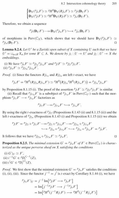
8.2 Intersection cohomology theory 205{DX(pj∗F˙) � pH 0DX(Rj∗F˙) � pj!(DU F˙)DX(pj!F˙) � pH 0DX(Rj!F˙) � pj∗(DU F˙).
Therefore, we obtain a sequence
pj!(DU F˙)�DX(pj!∗F˙) ↪−→ pj∗(DU F˙)of morphisms in Perv(CX), which shows that we should have DX(pj!∗F˙) �pj!∗(DU F˙). ��Lemma 8.2.4. Let U ′ be a Zariski open subset of X containing U such that we haveU ′ = �α∈B ′Xα for some B ′ ⊂ A. We denote by j1 : U → U ′ and j2 : U ′ → X theembeddings.
(i) We have pj∗F˙ � pj2∗pj1∗F˙ and pj!F˙ � pj2!pj1!F .(ii) pj!∗F˙ � pj2!∗pj1!∗F .
Proof. (i) Since the functors Rj1∗ and Rj2∗ are left t-exact, we have
pj∗F˙ = pH 0(Rj2∗Rj1∗F˙) � pH 0(Rj2∗pH 0(Rj1∗F˙)) = pj2∗pj1∗F˙by Proposition 8.1.15 (i). The proof of the assertion pj!F˙ � pj2!pj1!F˙ is similar.
(ii) Recall that pj1!∗F˙ is a subobject of pj1∗F˙ in Perv(CU ′) such that the mor-phism pj1!F˙ −→ pj1∗F˙ factorizes as
pj1!F˙�pj1!∗F˙ ↪−→ pj1∗F .
By using the right t-exactness of pj2! (Propositions 8.1.43 (ii) and 8.1.15 (ii)) and theleft t-exactness of pj2∗ (Proposition 8.1.43 (i) and Proposition 8.1.15 (ii)) we obtain
pj!F˙ = pj2! ◦ pj1!F˙�pj2! ◦ pj1!∗F˙�pj2!∗ ◦ pj1!∗F˙↪−→ pj2∗ ◦ pj1!∗F˙ ↪−→ pj2∗ ◦ pj1∗F˙ = pj∗F .
It follows that we have pj2!∗ ◦ pj1!∗F˙ � pj!∗F . ��Proposition 8.2.5. The minimal extension G˙ = pj!∗F˙ of F˙ ∈ Perv(CU ) is charac-terized as the unique perverse sheaf on X satisfying the conditions
(i) G˙|U � F ,(ii) i−1G˙ ∈ pD
�−1c (Z),
(iii) i!G˙ ∈ pD�1c (Z).
Proof. We first show that the minimal extension G˙ = pj!∗F˙ satisfies the conditions(i), (ii), (iii). Since the functor j−1 = j ! is t-exact by Corollary 8.1.44 (i), we have
pj!∗F˙|U = j−1 Im[pj!F˙ −→ pj∗F˙]
= Im[j−1pj!F˙ −→ j−1pj∗F˙]
= Im[pH 0(j−1Rj !F˙) −→ pH 0(j−1Rj∗F˙)]

206 8 Perverse Sheaves
= Im[F˙ −→ F˙]
= F .
Hence the condition (i) is satisfied. By the distinguished triangle
j!j−1G˙ −→ G· −→ i∗i−1G˙ +1−→in Db
c (X) we obtain an exact sequence
pH 0(j!j−1G˙) −→ pH 0(G˙) −→ pH 0(i∗i−1G˙) −→ pH 1(j!j−1G˙).By the definition of G· we have pH 0(G˙) = pj!∗F ·. By (i) we have j−1G˙ =F ·, and hence pH 0(j!j−1G˙) = pj!F ·. Moreover, we have pH 1(j!j−1G˙) = 0 byProposition 8.1.43 (ii). Finally, the canonical morphism pj!F · −→ pj!∗F · is anepimorphism by the definition of pj!∗. Therefore, we obtain pH 0(i∗i−1G˙) = 0 bythe above exact sequence. Since i∗ is t-exact, we have pH 0(i−1G˙) = 0. Since i−1 isright t-exact, we have i−1G˙ ∈ pD≤0
c (Z). It follows that i−1G˙ ∈ pD�−1c (Z). Hence
the condition (ii) is satisfied. The condition (iii) can be checked similarly to (ii) byusing the distinguished triangle
i∗i!G˙ −→ G· −→ Rj∗j−1G˙ +1−→ .
Let us show that G˙ ∈ Perv(CX) satisfying the conditions (i), (ii), (iii) is canon-ically isomorphic to pj!∗F ·. Since j−1(= j !) is left adjoint to Rj∗ and right adjointto j!, we obtain canonical morphisms j!F · −→ G· −→ Rj∗F · in Db
c (X). Hence weobtain canonical morphisms pj!F · −→ G· −→ pj∗F · in Perv(CX). It is sufficient toshow that pj!F · −→ G· is an epimorphism and G· −→ pj∗F · is a monomorphismin Perv(CX). We only show that pj!F · −→ G· is an epimorphism (the proof of theremaining assertion is similar). Since the cokernel of pj!F · −→ G· is supported byZ, there exists an exact sequence
pj!F · −→ G· −→ i∗H · −→ 0
for some H · ∈ Perv(CZ) (Corollary 8.1.44 (ii)). Since i−1 is right t-exact, we havean exact sequence pi−1G· −→ pi−1i∗H · −→ 0. By Corollary 8.1.44 (ii) we havepi−1i∗H · = i−1i∗H · = H ·. Moreover, by our assumption (ii) we have pi−1G· = 0.It follows that H · = 0, and hence pj!F · −→ G· is an epimorphism. ��Corollary 8.2.6. Assume that X is smooth. Then for any local system L ∈ Loc(X)
on X we have L[dX] � pj!∗(L|U [dX]).Proof. By Proposition 8.2.5 it is sufficient to show i−1L[dX] ∈ pD
�−1c (Z) and
i!L[dX] ∈ pD�1c (Z). By dZ < dX we easily see that i−1L[dX] ∈ pD
�−1c (Z).
Furthermore, we have
i!L[dX] � i!DXDX(L[dX])� DXi−1(L∗[dX]) ∈ pD�1
c (X),
where L∗ is the dual local system of L. ��
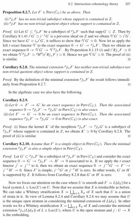
8.2 Intersection cohomology theory 207
Proposition 8.2.7. Let F˙ ∈ Perv(CU ) be as above. Then
(i) pj∗F · has no non-trivial subobject whose support is contained in Z.(ii) pj!F · has no non-trivial quotient object whose support is contained in Z.
Proof. (i) Let G˙ ⊂ pj∗F · be a subobject of pj∗F · such that supp G˙ ⊂ Z. Then byCorollary 8.1.41 i!G˙ � i−1G˙ is a perverse sheaf on Z and we obtain pi!G˙ � i!G .Since we have G˙ � i∗i!G , it suffices to show that pi!G˙ � 0. Now let us apply theleft t-exact functor pi! to the exact sequence 0 → G˙ → pj∗F ·. Then we obtain anexact sequence 0 → pi!G˙ → pi!pj∗F ·. By Proposition 8.1.15 (i) and i!Rj∗F · � 0we obtain pi!pj∗F · � pH 0(i!Rj∗F ·) � 0. Hence we get pi!G˙ � 0. The proof of (ii)is similar. ��Corollary 8.2.8. The minimal extension pj!∗F˙ has neither non-trivial subobject nornon-trivial quotient object whose support is contained in Z.
Proof. By the definition of the minimal extension pj!∗F˙ the result follows immedi-ately from Proposition 8.2.7. ��
In the algebraic case we also have the following.
Corollary 8.2.9.(i) Let 0 → F˙ → G˙ be an exact sequence in Perv(CU ). Then the associated
sequence 0 → pj!∗F˙ → pj!∗G˙ in Perv(CX) is also exact.(ii) Let F˙ → G˙ → 0 be an exact sequence in Perv(CU ). Then the associated
sequence pj!∗F˙ → pj!∗G˙ → 0 in Perv(CX) is also exact.
Proof. (i) Since the kernel K˙ of the morphism pj!∗F˙ → pj!∗G˙ is a subobject ofpj!∗F˙ whose support is contained in Z, we obtain K˙ � 0 by Corollary 8.2.8. Theproof of (ii) is similar. ��Corollary 8.2.10. Assume that F˙ is a simple object in Perv(CU ). Then the minimalextension pj!∗F˙ is also a simple object in Perv(CX).
Proof. Let G˙ ⊂ pj!∗F˙ be a subobject of pj!∗F˙ in Perv(CX) and consider the exactsequence 0 → G˙ → pj!∗F˙ → H˙ → 0 associated to it. If we apply the t-exactfunctor j ! = j−1 to it, then we obtain an exact sequence 0 → j−1G˙ → F˙ →j−1H˙ → 0. Since F˙ is simple, j−1G˙ or j−1H˙ is zero. In other words, G˙ or H˙is supported by Z. It follows from Corollary 8.2.8 that G˙ or H˙ is zero. ��
Now we focus our attention on the case where U is smooth and F · = L[dX] for alocal system L ∈ Loc(U) on U . Note that we assume that X is irreducible as before.We can take a Whitney stratification X = ⊔
α∈A Xα of X such that U is a unionof strata in it. In view of Lemma 8.2.4 and Corollary 8.2.6 we may assume that U
is the unique open stratum in considering the minimal extension of L[dX]. In otherwords we fix a Whitney stratification X = ⊔
α∈A Xα of X and consider the minimalextension pj!∗(L[dX]) of L ∈ Loc(U), where U is the open stratum and j : U → X
is the embedding.
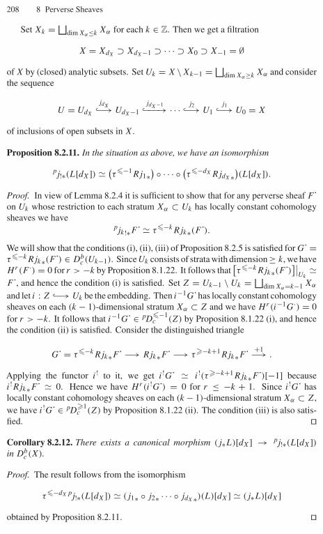
208 8 Perverse Sheaves
Set Xk = ⊔dim Xα≤k Xα for each k ∈ Z. Then we get a filtration
X = XdX⊃ XdX−1 ⊃ · · · ⊃ X0 ⊃ X−1 = ∅
of X by (closed) analytic subsets. Set Uk = X \Xk−1 = ⊔dim Xα≥k Xα and consider
the sequence
U = UdX
jdX↪−→ UdX−1 ↪
jdX−1−−−→ · · · j2↪−→ U1
j1↪−→ U0 = X
of inclusions of open subsets in X.
Proposition 8.2.11. In the situation as above, we have an isomorphism
pj!∗(L[dX]) � (τ�−1Rj1∗
) ◦ · · · ◦ (τ�−dXRjdX ∗)(L[dX]).
Proof. In view of Lemma 8.2.4 it is sufficient to show that for any perverse sheaf F˙on Uk whose restriction to each stratum Xα ⊂ Uk has locally constant cohomologysheaves we have
pjk !∗F˙ � τ�−kRjk∗(F˙).We will show that the conditions (i), (ii), (iii) of Proposition 8.2.5 is satisfied for G˙ =τ�−kRjk∗(F˙) ∈ Db
c (Uk−1). Since Uk consists of strata with dimension ≥ k, we haveHr(F ·) = 0 for r > −k by Proposition 8.1.22. It follows that
[τ�−kRjk∗(F˙)]∣∣
Uk�
F , and hence the condition (i) is satisfied. Set Z = Uk−1 \ Uk = ⊔dim Xα=k−1 Xα
and let i : Z ↪−→ Uk be the embedding. Then i−1G˙has locally constant cohomologysheaves on each (k − 1)-dimensional stratum Xα ⊂ Z and we have Hr(i−1G·) = 0for r > −k. It follows that i−1G˙ ∈ pD
�−1c (Z) by Proposition 8.1.22 (i), and hence
the condition (ii) is satisfied. Consider the distinguished triangle
G˙ = τ�−kRjk∗F˙ −→ Rjk∗F˙ −→ τ�−k+1Rjk∗F˙ +1−→ .
Applying the functor i! to it, we get i!G˙ � i!(τ�−k+1Rjk∗F˙)[−1] becausei!Rjk∗F˙ � 0. Hence we have Hr(i!G˙) = 0 for r ≤ −k + 1. Since i!G˙ haslocally constant cohomology sheaves on each (k − 1)-dimensional stratum Xα ⊂ Z,we have i!G˙ ∈ pD
�1c (Z) by Proposition 8.1.22 (ii). The condition (iii) is also satis-
fied. ��Corollary 8.2.12. There exists a canonical morphism (j∗L)[dX] → pj!∗(L[dX])in Db
c (X).
Proof. The result follows from the isomorphism
τ�−dX pj!∗(L[dX]) � (j1∗ ◦ j2∗ · · · ◦ jdX ∗)(L)[dX] � (j∗L)[dX]obtained by Proposition 8.2.11. ��
8.2 Intersection cohomology theory 209
Definition 8.2.13. For an irreducible algebraic variety (resp. an irreducible analyticspace) X we define its intersection cohomology complex ICX˙ ∈ Perv(CX) by
ICX˙ = pj!∗(CXanreg
[dX]) (resp. ICX˙ = pj!∗(CXreg [dX]),where Xreg denotes the regular part of X and j : Xreg ↪−→ X is the embedding.
By Proposition 8.2.3 we have the following.
Theorem 8.2.14. We have DX(ICX˙) = ICX .
Proposition 8.2.15. There exist canonical morphisms
CX −→ ICX˙[−dX] −→ ωX˙[−2dX]in Db
c (X).
Proof. By Corollary 8.2.12 there exists a natural morphism CX −→ ICX˙[−dX]. Bytaking the Verdier dual we obtain a morphism ICX˙[dX] −→ ωX . ��Definition 8.2.16. Let X be an irreducible analytic space. For i ∈ Z we set{
IH i(X) := Hi(R�(X, ICX˙[−dX])),IH i
c (X) := Hi(R�c(X, ICX˙[−dX])).
We call IH i(X) (resp. IH ic (X)) the ith intersection cohomology group (resp. the ith
intersection cohomology group with compact supports) of X.
The following theorem is one of the most important results in intersection coho-mology theory.
Theorem 8.2.17. Let X be an irreducible analytic space of dimension d. Then wehave the generalized Poincaré duality
IH i(X) � [IH 2d−i
c (X)]∗
for any 0 ≤ i ≤ 2d.
Proof. Let aX : X�{pt} be the unique morphism from X to the variety {pt}consisting of a single point. Then we have an isomorphism
RHomC(RaX !ICX˙, C) � RaX∗RHomCX(ICX˙, ωX˙)
in Db({pt}) � Db(Mod(C)) by the Poincaré–Verdier duality theorem. SinceRHomCX
(ICX˙, ωX˙) = DX(ICX˙) � ICX˙ by Theorem 8.2.14, we get an isomor-phism [
R�c(X, ICX˙)]∗ � R�(X, ICX˙)By taking the (i − d)th cohomology groups of both sides, we obtain the desiredisomorphism. ��

210 8 Perverse Sheaves
In what follows, let us set Hi(X) = Hi(X, CX) and Hic (X) = Hi
c (X, CX). Bythe Verdier duality theorem we have an isomorphism H−i (X, ωX˙) � [Hi
c (X)]∗ forany i ∈ Z. This hypercohomology group H−i (X, ωX˙) is called the ith Borel–Moorehomology group of X and denoted by HBM
i (X). If X is complete (or compact), thenHBM
i (X) is isomorphic to the usual homology group Hi(X) = Hi(X, C) of X. ByProposition 8.2.15 we obtain the following.
Proposition 8.2.18. There exist canonical morphisms
Hi(X) −→ IH i(X) −→ HBM2dX−i (X).
for any i ∈ Z.
The morphism Hi(X) −→ HBM2dX−i (X) can be obtained more directly as fol-
lows. Recall that the top-dimensional Borel–Moore homology group HBM2dX
(X) =[H 2dX
c (X)]∗ � C of X contains a canonical generator [X] called the fundamentalclass of X (see, for example, Fulton [F, Section 19.1]). Then by the cup product
Hi(X) × H 2dX−ic (X) −→ H 2dX
c (X)
and the morphism H2dXc (X) −→ C obtained by the fundamental class [X] ∈
[H 2dXc (X)]∗ we obtain a bilinear map
Hi(X) × H 2dX−ic (X) −→ C.
This gives a morphism Hi(X) −→ HBM2dX−i (X) = [H 2dX−i
c (X)]∗.
Proposition 8.2.19. Let X be a projective variety with isolated singular points. Thenwe have
IH i(X) =
⎧⎪⎪⎪⎪⎨⎪⎪⎪⎪⎩Hi(Xreg) 0 ≤ i < dX
Im[HdX(X) −→ HdX(Xreg)] i = dX
Hi(X) dX < i ≤ 2dX.
In particular we have Hi(Xreg) � H 2dX−i (X) for any 0 ≤ i < dX.
Proof. Let p1, p2, . . . , pk be the singular points of X and j : Xreg ↪−→ X theembedding. Then X = Xreg � (�k
i=1{pi}) is a Whitney stratification of X and wehave ICX˙[−dX] � τ�dX−1(Rj∗CXreg). Hence we obtain a distinguished triangle
ICX˙[−dX] −→ Rj∗CXreg −→ τ�dX(Rj∗CXreg)+1−→ .
Applying the functor R�(X, •), we easily see that
IH i(X) = Hi(X, ICX˙[−dX]) � Hi(Xreg)

8.2 Intersection cohomology theory 211
for 0 ≤ i < dX and the morphism
IHdX(X) = HdX(X, ICX˙[−dX]) ↪−→ HdX(Xreg)
is injective. Now let us embed the canonical morphism CX −→ ICX˙[−dX] (Propo-sition 8.2.15) into a distinguished triangle
CX −→ ICX˙[−dX] −→ F˙ +1−→ .
Then F˙ is supported by the zero-dimensional subset �ki=1{pi} of X and Hi(F˙) = 0
for any i ≥ dX. Therefore, applying R�(X, •) to this distinguished triangle, weobtain
Hi(X) � IH i(X) = Hi(X, ICX˙[−dX])for dX < i ≤ 2dX and the morphism
HdX(X)�IHdX(X) = HdX(X, ICX˙[−dX])is surjective. This completes the proof. ��
For some classes of varieties with mild singularities, intersection cohomologygroups are isomorphic to the usual cohomology groups. For example, let us recallthe following classical notion.
Definition 8.2.20. Let X be an algebraic variety or an analytic space. We say that X
is rationally smooth (or a rational homology “manifold’’) if for any point x ∈ X wehave
Hi{x}(X, CX) =⎧⎨⎩
C i = 2dX
0 otherwise.
By definition, rationally smooth varieties are pure-dimensional. Smooth varietiesare obviously rationally smooth. Typical examples of rationally smooth varieties withsingularities are complex surfaces with Kleinian singularities and moduli spaces ofalgebraic curves. More generally V -manifolds are rationally smooth. It is known thatthe usual cohomology groups of a rationally smooth variety satisfy Poincaré duality(see Corollary 8.2.22 below) and the hard Lefschetz theorem.
Proposition 8.2.21. Let X be a rationally smooth irreducible analytic space. Then thecanonical morphisms CX → ωX˙[−2dX] and CX → ICX˙[−dX] are isomorphisms.
Proof. Let i{x} : {x} ↪−→ X be the embedding. Then we have
i−1{x}ωX˙ = i−1
{x}DX(CX) � D{x}i!{x}(CX) � RHomC(R�{x}(X, CX), C)
and hence an isomorphism
Hj−2dX [i−1{x}ωX˙] � [H 2dX−j
{x} (X, CX)]∗

212 8 Perverse Sheaves
for any j ∈ Z. Then the isomorphism CX � ωX˙[−2dX] follows from these iso-morphisms and the rationally smoothness of X. Now let us set F˙ := CX[dX] �ωX˙[−dX] ∈ Db
c (X). Then the complex F˙ satisfies the condition DX(F˙) � F .Therefore, by Proposition 8.2.5 we can easily show that F˙ is isomorphic to the in-tersection cohomology complex ICX . ��Corollary 8.2.22. Let X be a rationally smooth irreducible analytic space. Then wehave an isomorphism Hi(X) � IH i(X) for any i ∈ Z.
Definition 8.2.23. Let X be an irreducible algebraic variety or an irreducible analyticspace. Let U be a Zariski open dense subset of Xreg and j : U → X the embedding.For a local system L ∈ Loc(U) on U we set
ICX(L)˙ = pj!∗(L[dX]) ∈ Perv(CX)
and call it a twisted intersection cohomology complex of X. We sometimes denoteICX(L)˙[−dX] by πL .
Let X be an algebraic variety or an analytic space. Consider an irreducible closedsubvariety Y of X and a simple object L of Loc(Y0) (i.e., an irreducible local systemon Y0), where Y0 is a smooth Zariski open dense subset of Y . Then the minimalextension ICY (L)˙ of the locally constant perverse sheaf L[dY ] to Y can be naturallyconsidered as a perverse sheaf on X by Corollary 8.1.44 (ii). By Corollary 8.2.10and Lemma 8.2.24 below this perverse sheaf on X is a simple object in Perv(CX).Moreover, it is well known that any simple object in Perv(CX) can be obtained inthis way (see [BBD]).
Lemma 8.2.24. Let L be an irreducible local system on a smooth irreducible vari-ety X. Then the locally constant perverse sheaf L[dX] on X is a simple object inPerv(CX).
Proof. Let 0 → F1˙ → L[dX] → F2˙ → 0 be an exact sequence in Perv(CX).Choose a Zariski open dense subset U of X on which F1˙ and F2˙ have locallyconstant cohomology sheaves and set j : U ↪−→ X. Then by Lemma 8.1.23 thereexist local systems M1, M2 on U such that F1˙|U � M1[dX], F2˙|U � M2[dX]. Hencewe obtain an exact sequence 0 → M1 → L|U → M2 → 0 of local systems on U .Since M1 can be extended to the local system j∗M1 ⊂ j∗(L|U ) � L of the same rankon X, it follows from the irreducibility of L that M1 or M2 is zero. Namely, F1˙ orF2˙ is supported by Z = X \ U . Since L[dX] � pj!∗(L|U [dX]) by Corollary 8.2.6,F1˙ or F2˙ should be zero by Corollary 8.2.8. ��Remark 8.2.25. Assume that X is a complex manifold. For a C×-invariantLagrangian analytic subset � of the cotangent bundle T ∗X denote by Perv�(CX)
the subcategory of Perv(CX) consisting of objects whose micro-supports are con-tained in �. From the results in some simple cases it is generally expected thatfor any � ⊂ T ∗X as above there exists a finitely presented algebra R such thatthe category Perv�(CX) is equivalent to that of finite-dimensional representations
8.2 Intersection cohomology theory 213
of R. In some special (but important) cases this algebraic (or quiver) descriptionof the category Perv�(CX) was established by [GGM]. Recently this problem hasbeen completely solved for any smooth projective variety X and any � ⊂ T ∗X byS. Gelfand–MacPherson–Vilonen [GMV].
Now we state the decomposition theorem due to Beilinson–Bernstein–Deligne–Gabber (see [BBD]) without proofs.
Theorem 8.2.26 (Decomposition theorem). For a proper morphism f : X −→ Y
of algebraic varieties, we have
Rf ∗[ICX˙] �
finite⊕k
ik∗ICYk(Lk)˙[lk]. (8.2.1)
Here for each k, Yk is an irreducible closed subvariety of Y , ik : Yk ↪−→ Y is theembedding, Lk ∈ Loc(Y ′
k) for some smooth Zariski open subset Y ′k of Yk , and lk is an
integer.
The proof relies on a deep theory of weights for étale perverse sheaves in positivecharacteristics. This result can be extended to analytic situation via the theory ofHodge modules (see Section 8.3 below).
Corollary 8.2.27. Let X be a projective variety and π : X → X a resolution ofsingularities of X. Then IH i(X) is a direct summand of Hi(X) for any i ∈ Z.
Proof. By the decomposition theorem we have
Rπ∗(CX[dX]) � ICX˙ ⊕ F˙for some F˙ ∈ Db
c (X), from which the result follows. ��Remark 8.2.28. The decomposition theorem has various important applications ingeometric representation theory of reductive algebraic groups. For details we referthe reader to Lusztig [L2] and Chriss–Ginzburg [CG].
In general the direct image of a perverse sheaf is not necessarily a perverse sheaf.We will give a sufficient condition on a morphism f : X → Y so that Rf∗(ICX˙) isperverse.
Definition 8.2.29. Let f : X → Y be a dominant morphism of irreducible algebraicvarieties. We say that f is small (resp. semismall) if the condition codimY {y ∈ Y |dim f −1(y) ≥ k} > 2k (resp. codimY {y ∈ Y | dim f −1(y) ≥ k} ≥ 2k) is satisfiedfor any k ≥ 1.
Note that if f : X → Y is semismall then there exists a smooth open dense subsetU ⊂ Y such that f |f −1(U): f −1(U) → U is a finite morphism. In particular wehave dX = dY .
214 8 Perverse Sheaves
Proposition 8.2.30. Let f : X → Y be a dominant proper morphism of irreduciblealgebraic varieties. Assume that X is rationally smooth.
(i) Assume that f is semismall. Then the direct image Rf∗(CXan [dX]) of the constantperverse sheaf CXan [dX] � ICX˙ is a perverse sheaf on Y .
(ii) Assume that f is small. Then we have an isomorphism Rf∗(CXan [dX]) �ICY (L)˙ for some L ∈ Loc(U), where U is a smooth open subset of Y .
Proof. (i) By DY Rf∗ � Rf∗DX (f is proper) it suffices to check the condi-tion Rf∗(CXan [dX]) ∈ pD
�0c (X). This follows easily from Rj f∗(CXan )y =
Hj (f −1(y), C) and the fact that Hj (f −1(y), C) = 0 for j > 2 dim f −1(y).(ii) By our assumption there exists an open subset U ⊂ Y such that f |f −1(U):
f −1(U) → U is a finite morphism. If necessary, we can shrink U so that U issmooth and f∗CXan |U an ∈ Loc(U). We denote this local system by L. Set Z = Y \U
and let i : Z ↪→ Y be the embedding. By Proposition 8.2.5 we have only to showthat i−1Rf∗(CXan [dX]) ∈ pD
�−1c (Z) and i!Rf∗(CXan [dX]) ∈ pD
�1c (Z). Again by
DY Rf∗ � Rf∗DX it is enough to check only the condition i−1Rf∗(CXan [dX]) ∈pD
�−1c (Z). This can be shown by the argument used in the proof of (i). ��
Recall that the normalization π : X → X of a projective variety X is a finite map
which induces an isomorphism π |π−1Xreg: π−1Xreg −→∼ Xreg.
Corollary 8.2.31. Let X be a projective variety and π : X → X its normalization.Then we have an isomorphism
Rπ∗[ICX˙] � ICX .
In particular, there exists an isomorphism IH i(X) � IH i(X) for any i ∈ Z.
Since the normalization π : C → C of an algebraic curve C is smooth, we obtainan isomorphism IH i(C) � Hi(C) for any i ∈ Z. However, this is not always truein higher-dimensional cases.
Example 8.2.32. Let C be an irreducible plane curve defined by C = {(x0 : x1 : x2)
∈ P2(C)|x30 + x3
1 = x0x1x2}. Since C has an isolated singular point, we obtain
IH i(C) =
⎧⎪⎪⎪⎪⎨⎪⎪⎪⎪⎩C i = 0
0 i = 1
C i = 2
by Proposition 8.2.19. In this case the normalization C of C is isomorphic to P1(C)
and hence we observe that IH i(C) � Hi(C) for any i ∈ Z.
8.2 Intersection cohomology theory 215
Remark 8.2.33. Proposition 8.2.30 has important consequences in representationtheory. For example, let G be a semisimple algebraic group over C and B ⊂ G
a Borel subgroup (see Chapter 9 for the definitions). For the flag variety X = G/B ofG let us set G = {(g, x) ∈ G×X | gx = x} ⊂ G×X. Then G is a smooth complexmanifold because the second projection G → X is a fiber bundle on X. Furthermore,it turns out that the first projection f : G → G is small (see Lusztig [L1]). Therefore,via the Riemann–Hilbert correspondence, Proposition 8.2.30 implies that
Hj
∫f
OG = 0 for j = 0.
The remaining non-zero term H 0∫
fOG is a regular holonomic system on G and
coincides with the one satisfied by the characters of representations (invariant distri-butions) of a real form of G (see [HK1]). Harish-Chandra obtained many importantresults in representation theory through the detailed study of this system of equations.We also note that Proposition 8.2.30 and Theorem 8.2.36 below play crucial roles inthe recent progress of the geometric Langlands program (see, for example, [MV]).
We end this section by presenting a beautiful application of the decompositiontheorem due to Borho–MacPherson [BM] on the explicit description of the directimages of constant perverse sheaves. Let f : X → Y be a dominant projectivemorphism of irreducible algebraic varieties. Then by a well-known result in analyticgeometry (see, for example, Thom [Th, p. 276]), there exists a complex stratificationY = �α∈AYα of Y by connected strata Yα’s such that f |f −1Yα
: f −1Yα → Yα
is a topological fiber bundle with the fiber Fα := f −1(yα) (yα ∈ Yα). Let usassume, moreover, that f is semismall. Then we have codimY Yα ≥ 2 dim Fα forany α ∈ A. Note that for any i > 2 dim Fα we have Hi(Fα) = 0. In particular[HiRf ∗(CX)]|Yα = 0 for any i > codimY Yα . Set cα = codimY Yα and denote byLα the local system [Hcα Rf ∗(CX)]|Yα on Yα .
Definition 8.2.34. We say that a stratum Yα is relevant if the condition cα = 2 dim Fα
holds.
We easily see that f is small if and only if the only relevant stratum is the opendense one. Moreover, a stratum Yα is relevant if and only if Lα = 0. For a relevantstratum Yα the top-dimensional cohomology group Hcα (Fα) � (Lα)yα of the fiberFα has a basis corresponding to the dFα -dimensional irreducible components of Fα .The fundamental group of Yα acts on the C-vector space Hcα (Fα) � (Lα)yα bypermutations of these irreducible components. This action completely determinesthe local system Lα . For each α ∈ A let
Lα =⊕
φ
(Lφ)⊕mφ
be the irreducible decomposition of the local system Lα , where φ ranges through theset of all irreducible representations of the fundamental group of Yα and mφ ≥ 0 isthe multiplicity of the irreducible local system Lφ corresponding to φ.
216 8 Perverse Sheaves
Definition 8.2.35. We say that a pair (Yα, φ) of a stratum Yα and an irreducible rep-resentation of the fundamental group of Yα is relevant if the stratum Yα is relevantand mφ = 0.
Theorem 8.2.36 (Borho–MacPherson [BM]). In the situation as above, assume,moreover, that X is rationally smooth. Then the direct image Rf ∗(CX[dX]) of theconstant perverse sheaf CX[dX] � ICX˙ is explicitly given by
Rf ∗(CX[dX]) �⊕
(Yα,φ)
[iα∗ICZα (Lφ)˙]⊕mφ ,
where (Yα, φ) ranges through the set of all relevant pairs, Zα is the closure of Yα andiα : Zα ↪−→ Y is the embedding.
Proof. By Proposition 8.2.30 the direct image Rf ∗(CX[dX]) is a perverse sheaf onY . By the decomposition theorem we can prove recursively that on each strata Yβ itis written more explicitly as
Rf ∗(CX[dX]) �⊕
(Yα,φ)
[iα∗ICZα (Lφ)˙]⊕nφ ,
where (Yα, φ) ranges through the set of all pairs of Yα and irreducible representations φ
of the fundamental group of Yα , and nφ are some non-negative integers. Indeed, let Yα0
be the unique open dense stratum in Y . Then on Yα0 the direct image Rf ∗(CX[dX])is obviously written as
Rf ∗(CX[dX]) �⊕
(Yα0 ,φ)
(Lφ[dX])⊕mφ ,
where (Yα0 , φ) ranges through the set of relevant pairs. Namely, for any pair (Yα, φ)
such that α = α0 we have nφ = mφ . Let Yα1 be a stratum such that codimY Yα1 = 1.Since HiRf ∗(CX[dX]) = 0 on Yα1 for i = −dX by the semismallness of f , for anypair (Yα, φ) such that α = α1 we must have nφ = 0. Therefore, on Yα0 � Yα1 weobtain an isomorphism
Rf ∗(CX[dX]) �⊕
(Yα0 ,φ)
[iα0∗ICZα0(Lφ)˙]⊕mφ ,
where (Yα0 , φ) ranges through the set of relevant pairs. By repeating this argument,we can finally prove the theorem. ��Remark 8.2.37. By Theorem 8.2.36 we can geometrically construct and study repre-sentations of Weyl groups of semisimple algebraic groups. This is the so-called theoryof Springer representations. For this very important application of Theorem 8.2.36,see Borho–MacPherson [BM]. As another subject where Theorem 8.2.36 is appliedeffectively we also point out the work by Göttsche [Go] computing the Betti numbersof Hilbert schemes of points of algebraic surfaces. Inspired by this result Nakajima[Na1] and Grojnowski [Gr] found a beautiful symmetry in the cohomology groupsof these Hilbert schemes (see [Na2] for the details).
8.3 Hodge modules 217
8.3 Hodge modules
8.3.1 Motivation
Let k an the algebraic closure of the prime field Fp of characteristic p. Startingfrom a given separated scheme X of finite type over Z, we can construct by basechanges, the schemes XC = X ⊗Z C over C and Xk = X ⊗Z k over k. Thescheme Xk is regarded as the counterpart of XC in positive characteristic. We havecohomology groups H ∗(Xan
C, Q), H ∗
c (XanC
, Q) for the underlying analytic space XanC
of XC; the corresponding notions in positive characteristic are the so-called l-adicétale cohomology groups H ∗(Xk, Ql ), H ∗
c (Xk, Ql ) (l is a prime number differentfrom p). More precisely, under some suitable conditions on X over Z we have theisomorphisms
H ∗(XanC , Q) ⊗Q Ql � H ∗(Xk, Ql ), H ∗
c (XanC , Q) ⊗Q Ql � H ∗
c (Xk, Ql ),
which show that the étale topology for Xk corresponds to the classical topology forXC. This correspondence can be extended to the level of local systems and perversesheaves on Xan
Cand Xk .
For Xk we have the Frobenius morphism, which is an operation peculiar to the caseof positive characteristic. This allows us, compared with the case of XC, to developa more detailed theory on Xk by considering étale local systems and étale perversesheaves endowed with the action of the Frobenius morphisms (Weil sheaves). Thatis the theory of weights for étale sheaves, which played an important role in the proofof the Weil conjecture [De3], [BBD].
However, Grothendieck’s philosophy predicted the existence of the theory ofweights for objects over C. In the case of local systems, the theory of the variationof Hodge structures had been known as a realization of such a theory over C [De2].In the case of general perverse sheaves, a theory of weight which is based on theRiemann–Hilbert correspondence was constructed, and gave the final answer to thisproblem. This is the theory of Hodge modules due to Morihiko Saito [Sa1], [Sa3].
In this section, we present a brief survey on the theory of Hodge modules.
8.3.2 Hodge structures and their variations
In this subsection we discuss standard notions on Hodge structures. For more preciseexplanations, refer to [De2], [GS].
Let X be a smooth projective algebraic variety. The complexifications HC =Hn(Xan, C) of its rational cohomology groups H = Hn(Xan, Q) (n ∈ Z) can benaturally identified with the de Rham cohomology groups. Moreover, in such cases,a certain family { Hp,q | p, q ∈ N, p + q = n } of subspaces of HC is defined bythe theory of harmonic forms so that we have the Hodge decomposition
HC =⊕
p+q=n
Hp,q, H p,q = Hq,p.
218 8 Perverse Sheaves
Here we denote the complex conjugation map of HC with respect to H by h �→h (h ∈ HC). Let us set F p(HC) := ⊕
i≥p H i,n−i . Then F defines a decreasing
filtration of HC and the equality HC = F p ⊕ F n−p+1 holds for every p. We call itthe Hodge filtration of HC. Note that we can reconstruct the subspaces Hp,q fromthe Hodge filtration by using Hp,q = F p ∩ F q .
Therefore, it would be natural to define the notion of Hodge structures in thefollowing way. Let H be a finite-dimensional vector space over Q and HC its com-plexification. Denote by h �→ h (h ∈ HC) the complex conjugation map of HC andconsider a finite decreasing filtration F = { F p(HC) }p∈Z by subspaces in HC. Thatis, we assume that F p(HC)’s are subspaces of HC satisfying F p(HC) ⊃ F p+1(HC)
(∀p) and F p(HC) = {0}, F −p(HC) = HC (p � 0). For an integer n, we say thatthe pair (H, F ) is a Hodge structure of weight n if the condition
HC = F p ⊕ F n−p+1
holds for any p. The filtration F is called the Hodge filtration. In this case, if we setHp,q = F p ∩ F q , then we obtain the Hodge decomposition
HC =⊕
p+q=n
Hp,q, H p,q = Hq,p.
We can naturally define the morphisms between Hodge structures as follows. Giventwo Hodge structures (H, F ), (H ′, F ) of the same weight n, a linear map f : H →H ′ is called a morphism of Hodge structures if it satisfies the condition
f (F p(HC)) ⊂ F p(H ′C)
for any p. Here we used the same symbol f for the complexified map HC → H ′C
off . Thus we have defined the category SH(n) of the Hodge structures of weight n.The morphisms in SH(n) are strict with respect to the Hodge filtration F . Namely,for f ∈ HomSH(n)
((H, F ), (H ′, F )
)we always have
f (F p(HC)) = f (HC) ∩ F p(H ′C)
for any p ∈ Z, from which we see that SH(n) is an abelian category.Next let us explain the polarizations of Hodge structures. We say a Hodge struc-
ture (H, F ) ∈ SH(n) is polarizable if there exists a bilinear form S on HC satisfyingthe following properties:
(i) If n is even, S is symmetric. If n is odd, S is anti-symmetric.(ii) If p + p′ = n, we have S(Hp,n−p, Hp′,n−p′
) = 0.(iii) For any v ∈ Hp,n−p such that v = 0 we have (
√−1)n−2pS(v, v) > 0.
Denote by SH(n)p the full subcategory of SH(n) consisting of polarizable Hodgestructures of weight n. Then it turns out that SH(n)p is an abelian category, and anyobject from it can be expressed as a direct sum of irreducible objects.
As we have explained above, for a smooth projective algebraic variety X, a naturalHodge structure of weight n can be defined on Hn(Xan, Q); however, the situation is
8.3 Hodge modules 219
much more complicated for non-projective varieties with singularities. In such cases,the cohomology group Hn(Xan, Q) is a sort of mixture of the Hodge structures ofvarious weights. This is the theory of mixed Hodge structures due to Deligne.
Let us give the definition of mixed Hodge structures. Let H be a finite-dimensionalvector space over Q, F a finite decreasing filtration of HC and W = {Wn(H)}n∈Z
a finite increasing filtration of H . By complexifying W , we get an increas-ing filtration of HC, which we also denote by W . Then the complexification ofgrW
n (H) = Wn(H)/Wn−1(H) is identified with Wn(HC)/Wn−1(HC) and its de-creasing filtration is defined by
F p(Wn(HC)/Wn−1(HC)) = (Wn(HC) ∩ F p(HC) + Wn−1(HC))/Wn−1(HC).
We say that a triplet (H, F, W) is a mixed Hodge structure if for any n the filteredvector space grW
n (H, F ) := (grWn (H), F ) is a Hodge structure of weight n. We can
naturally define the morphisms between mixed Hodge structures, and hence the cate-gory SHM of mixed Hodge structures is defined. Let SHMp be the full subcategoryof SHM consisting of objects (H, F, W) ∈ SHM such that grW
n (H, F ) ∈ SH(n)p
for any n. They are abelian categories.Next we explain the notion of the variations of Hodge structures, which naturally
appears in the study of deformation (moduli) theory of algebraic varieties.Let f : Y → X be a smooth projective morphism between two smooth algebraic
varieties. Then the nth higher direct image sheaf Rnf an∗ (QY an ) is a local systemon Xan whose stalk at x ∈ X is isomorphic to Hn(f −1(x)an, Q). Since the fiberf −1(x) is a smooth projective variety, there exists a Hodge structure of weight n onHn(f −1(x)an, Q). Namely, the sheaf Rnf an∗ (QY an ) is a local system whose stalksare Hodge structures of weight n. Extracting properties of this local system, we cometo the definition of the variations of Hodge structures as follows.
Let X be a smooth algebraic variety and H a Q-local system on Xan. Then by atheorem of Deligne (Theorem 5.3.8), there is a unique (up to isomorphisms) regularintegrable connection M on X such that DR(M) = C ⊗Q H [dim X]. Let us denotethis regular integrable connection M by M(H). Assume that F = {F p(M(H))}p∈Z
is a finite decreasing filtration of M(H) by OX-submodules such that F p/F p+1 isa locally free OX-module for any p. Namely, F corresponds to a filtration of theassociated complex vector bundle by its subbundles. Since the complexification(Hx)C of the stalk Hx of H at x ∈ X coincides with C ⊗OX,x
M(H)x , a decreasingfiltration F(x) of (Hx)C is naturally defined by F . Now we say that the pair (H, F )
is a variation of Hodge structures of weight n if it satisfies the conditions
(i) For any x ∈ X, (Hx, F (x)) ∈ SH(n).(ii) For any p ∈ Z, we have �X · F p(M(H)) ⊂ F p−1(M(H)), where �X stands
for the sheaf of holomorphic vector fields on X.
The last condition is called Griffiths transversality. Also, we say that the variation ofHodge structures (H, F ) is polarizable if there exists a morphism
S : H ⊗QXan H −→ QXan
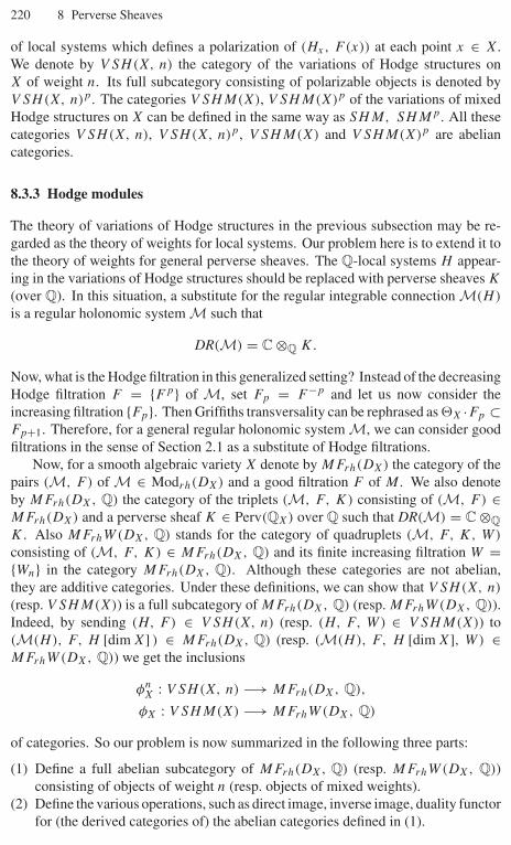
220 8 Perverse Sheaves
of local systems which defines a polarization of (Hx, F (x)) at each point x ∈ X.We denote by V SH(X, n) the category of the variations of Hodge structures onX of weight n. Its full subcategory consisting of polarizable objects is denoted byV SH(X, n)p. The categories V SHM(X), V SHM(X)p of the variations of mixedHodge structures on X can be defined in the same way as SHM, SHMp. All thesecategories V SH(X, n), V SH(X, n)p, V SHM(X) and V SHM(X)p are abeliancategories.
8.3.3 Hodge modules
The theory of variations of Hodge structures in the previous subsection may be re-garded as the theory of weights for local systems. Our problem here is to extend it tothe theory of weights for general perverse sheaves. The Q-local systems H appear-ing in the variations of Hodge structures should be replaced with perverse sheaves K
(over Q). In this situation, a substitute for the regular integrable connection M(H)
is a regular holonomic system M such that
DR(M) = C ⊗Q K.
Now, what is the Hodge filtration in this generalized setting? Instead of the decreasingHodge filtration F = {F p} of M, set Fp = F −p and let us now consider theincreasing filtration {Fp}. Then Griffiths transversality can be rephrased as �X ·Fp ⊂Fp+1. Therefore, for a general regular holonomic system M, we can consider goodfiltrations in the sense of Section 2.1 as a substitute of Hodge filtrations.
Now, for a smooth algebraic variety X denote by MFrh(DX) the category of thepairs (M, F ) of M ∈ Modrh(DX) and a good filtration F of M . We also denoteby MFrh(DX, Q) the category of the triplets (M, F, K) consisting of (M, F ) ∈MFrh(DX) and a perverse sheaf K ∈ Perv(QX) over Q such that DR(M) = C ⊗Q
K . Also MFrhW(DX, Q) stands for the category of quadruplets (M, F, K, W)
consisting of (M, F, K) ∈ MFrh(DX, Q) and its finite increasing filtration W ={Wn} in the category MFrh(DX, Q). Although these categories are not abelian,they are additive categories. Under these definitions, we can show that V SH(X, n)
(resp. V SHM(X)) is a full subcategory of MFrh(DX, Q) (resp. MFrhW(DX, Q)).Indeed, by sending (H, F ) ∈ V SH(X, n) (resp. (H, F, W) ∈ V SHM(X)) to(M(H), F, H [dim X] ) ∈ MFrh(DX, Q) (resp. (M(H), F, H [dim X], W) ∈MFrhW(DX, Q)) we get the inclusions
φnX : V SH(X, n) −→ MFrh(DX, Q),
φX : V SHM(X) −→ MFrhW(DX, Q)
of categories. So our problem is now summarized in the following three parts:
(1) Define a full abelian subcategory of MFrh(DX, Q) (resp. MFrhW(DX, Q))consisting of objects of weight n (resp. objects of mixed weights).
(2) Define the various operations, such as direct image, inverse image, duality functorfor (the derived categories of) the abelian categories defined in (1).

8.3 Hodge modules 221
(3) Show that the notions defined in (1), (2) satisfy the properties that deserves thename of the theory of weights. That is, prove basic theorems similar to those inthe theory of weights in positive characteristic.
Morihiko Saito tackled these problems for several years and gave a deci-sive answer. In [Sa1], Saito defined the full abelian subcategory MH(X, n) ofMFrh(DX, Q) consisting of the Hodge modules of weight n. He also gave thedefinition of the full abelian subcategory MH(X, n)p of MH(X, n) consisting ofpolarizable objects and proved its stability through the direct images associated toprojective morphisms. Next, in [Sa3], he defined the category MHM(X) of mixedHodge modules as a subcategory of MFrhW(DX, Q) and settled the above problems(2), (3). Since the definition of Hodge modules requires many steps, we do not givetheir definition here and explain only their properties.
We first present some basic properties of the categories MH(X, n) andMH(X, n)p following [Sa1]:
(p1) MH(X, n), MH(X, n)p are full subcategories of MFrh(DX, Q), and wehave MH (X, n)p ⊂ MH(X, n).
(p2) (locality) Consider an open covering X = ⋃λ∈� Uλ of X. For V ∈
MFrh(DX, Q) we have V ∈ MH(X, n) (resp. MH(X, n)p) if and only ifV|Uλ ∈ MH( Uλ, n) (resp. V|Uλ ∈ MH(Uλ, n)p).
(p3) All morphisms in MH(X, n) and MH(X, n)p are strict with respect to thefiltrations F .
We see from (p3) that MH(X, n) and MH(X, n)p are abelian categories. ForV = (M, F, K) ∈ MH(X, n) the support supp(M) of M is called the support ofV and we denote it by supp(V). This is a closed subvariety of X. Now let Z be anirreducible closed subvariety of X. We say V = (M, F, K) ∈ MH(X, n) has thestrict support Z if the support of V is Z and there is neither subobject nor quotientobject of V whose support is a non-empty proper subvariety of Z. Let us denoteby MHZ(X, n) the full subcategory of MH(X, n) consisting of objects having thestrict support Z. We also set MHZ(X, n)p = MHZ(X, n) ∩ MH(X, n)p. Thenwe have
(p4) MH(X, n) = ⊕Z MHZ(X, n), MH(X, n)p = ⊕
Z MHZ(X, n)p, whereZ ranges over the family of irreducible closed subvarieties of X.
If one wants to find a category satisfying only the conditions (p1)–(p4) one canset MH(X, n) = {0} for all X; however, the category MH(X, n) is really not trivial,as we will explain below.
For V = (M, F, K) ∈ MFrh(DX, Q) and an integer m we define V(m) ∈MFrh(DX, Q) by
V(m) = (M ⊗Q Q(m), F [m], K ⊗Q Q(m))
(the Tate twist of V), where Q(m) = (2π√−1)mQ ⊂ C and F [m]p = Fp−m. The
readers might feel it strange to write ⊗QQ(m); however, this notation is natural fromthe viewpoint of Hodge theory.
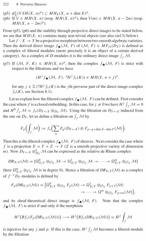
222 8 Perverse Sheaves
(p5) φnX(V SH(X, n)p) ⊂ MHX(X, n + dim X)p.
(p6) If V ∈ MH(X, n) (resp. MH(X, n)p), then V(m) ∈ MH(X, n − 2m) (resp.MH(X, n − 2m)p).
From (p5), (p6) and the stability through projective direct images to be stated below,we see that MH(X, n) contains many non-trivial objects (see also (m13) below).
Let f : X → Y be a projective morphism between two smooth algebraic varieties.Then the derived direct image f�(M, F ) of (M, F ) ∈ MFrh(DX) is defined asa complex of filtered modules (more precisely it is an object of a certain derivedcategory). As a complex of D-modules it is the ordinary direct image
∫f
M.
(p7) If (M, F, K) ∈ MH(X, n)p, then the complex f�(M, F ) is strict withrespect to the filtrations and we have
(Hj f�(M, F ), pHj f∗(K)) ∈ MH(Y, n + j)p.
for any j ∈ Z (pHj f∗(K) is the j th perverse part of the direct image complexf∗(K), see Section 8.1).
Let us explain how the filtered complex f�(M, F ) can be defined. First considerthe case where f is a closed embedding. In this case, for j = 0 we have Hj
∫f
M = 0
and H 0∫
fM = f∗(DY←X ⊗DX
M). Using the filtration on DY←X induced from
the one on DY , let us define a filtration on∫
fM by
Fp
(∫f
M)
:= f∗(∑
q
Fq(DY←X) ⊗ Fp−q+dim X−dim Y (M)).
Then this is the filtered complex f�(M, F ) of sheaves. Next consider the case wheref is a projection X = Y × Z → Y (Z is a smooth projective variety of dimensionm). Now DY←X ⊗L
DXM can be expressed as the relative de Rham complex
DRX/Y (M) = [�0X/Y ⊗OX
M → �1X/Y ⊗OX
M → · · · → �mX/Y ⊗OX
M](here �m
X/Y ⊗OXM is in degree 0). Hence a filtration of DRX/Y (M) as a complex
of f −1DY -modules is defined by
Fp(DRX/Y (M)) = [�0
X/Y ⊗OXFp(M) → �1
X/Y ⊗OXFp+1(M)
→ · · · → �m ⊗OXFp+m(M)
],
and its sheaf-theoretical direct image is f�(M, F ). Note that the complexf�(M, F ) is strict if and only if the morphism
Hj(Rf∗(Fp(DRX/Y (M)))
) −→ Hj(Rf∗(DRX/Y (M))
) = Hj
∫f
M
is injective for any j and p. If this is the case, Hj∫
fM becomes a filtered module
by the filtration
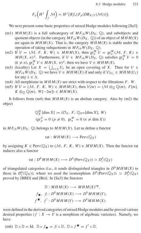
8.3 Hodge modules 223
Fp
(Hj
∫f
M)
= Hj(Rf∗(Fp(DRX/Y (M)))
).
We next present some basic properties of mixed Hodge modules following [Sa3]:
(m1) MHM(X) is a full subcategory of MFrhW(DX, Q), and subobjects andquotient objects (in the category MFrhW(DX, Q)) of an object of MHM(X)
are again in MHM(X). That is, the category MHM(X) is stable under theoperation of taking subquotients in MFrhW(DX, Q).
(m2) If V = (M, F, K, W) ∈ MHM(X), then grWn V = grW
n (M, F, K) ∈MH(X, n)p. Furthermore, if V ∈ MFrhW(DX, Q) satisfies grW
k V = 0(k = n), grW
n V ∈ MH(X, n)p, then we have V ∈ MHM(X).(m3) (locality) Let X = ⋃
λ∈� Uλ be an open covering of X. Then for V ∈MFrhW(DX, Q) we have V ∈ MHM(X) if and only if V|Uλ ∈ MHM(Uλ)
for any λ ∈ �.(m4) All morphisms in MHM(X) are strict with respect to the filtrations F, W .(m5) If V = (M, F, K, W) ∈ MHM(X), then V(m) = (M ⊗Q Q(m), F [m],
K ⊗Q Q(m), W [−2m]) ∈ MHM(X).
It follows from (m4) that MHM(X) is an abelian category. Also by (m2) theobject
QHX [dim X] := (OX, F, QXan [dim X], W)
(grFp = 0 (p = 0), grW
n = 0 (n = dim X))
in MFrhW(DX, Q) belongs to MHM(X). Let us define a functor
rat : MHM(X) −→ Perv(QX)
by assigning K ∈ Perv(QX) to (M, F, K, W) ∈ MHM(X). Then the functor ratinduces also a functor
rat : DbMHM(X) −→ Db(Perv(QX)) � Dbc (QX)
of triangulated categories (i.e., it sends distinguished triangles in DbMHM(X) tothose in Db
c (QX)), where we used the isomorphism Db(Perv(QX)) � Dbc (QX)
proved by [BBD] and [Bei]. In [Sa3] the functors
D : MHM(X) −→ MHM(X)op,
f�, f! : DbMHM(X) −→ DbMHM(Y),
f �, f ! : DbMHM(Y) −→ DbMHM(X)
were defined in the derived categories of mixed Hodge modules and he proved variousdesired properties (f : X → Y is a morphism of algebraic varieties). Namely, wehave
(m6) D ◦ D = Id, D ◦ f� = f! ◦ D, D ◦ f � = f ! ◦ D.

224 8 Perverse Sheaves
(m7) D ◦ rat = rat ◦D, f∗ ◦ rat = rat ◦f�, f! ◦ rat = rat ◦f!, f ∗ ◦ rat =rat ◦f �, f ! ◦ rat = rat ◦f !.
(m8) If f is a projective morphism, then f� = f!.
Let V ∈ DbMHM(X). We say that V has mixed weights ≤ n (resp. ≥ n) ifgrW
i HjV = 0 (i > j + n) (resp. grWi HjV = 0 (i < j + n)). Also V is said to have
a pure weight n if grWi HjV = 0 (i = j + n) holds. Now we have the following
results, which justify the name “theory of weights’’:
(m9) If V has mixed weights ≤ n (resp. ≥ n), then DV has mixed weights ≥ −n
(resp. ≤ −n).(m10) If V has mixed weights ≤ n, then f!V , f �V have mixed weights ≤ n.(m11) If V has mixed weights ≥ n, then f�V , f !V have mixed weights ≥ n.
Next we will explain the relation with the variations of mixed Hodge structures.
(m12) Let H ∈ V SHM(X)p. Then φX(H) ∈ MFrhW(DX, Q) is an object ofMHM(X) if and only if H is admissible in the sense of Kashiwara [Kas13].
This implies in particular that MHM(pt) = SHMp (the case when X is a one-pointvariety {pt}).
Finally, let us describe the objects in MHZ(X, n)p by using direct images (Z isan irreducible subvariety of X). Let U be a smooth open subset of Z and assumethat the inclusion map j : U ↪→ X is an affine morphism. For H ∈ V SH(U, n)p,j!φn
UH and j∗φnUH are objects in MHM(X) having weights ≤ n, ≥ n, respectively.
Therefore, if we set
j!∗φnUH = Im
[j!φn
UH −→ j∗φnUH
],
then j!∗φnUH is an object in MHM(X) having the pure weight n + dim Z (this func-
tor j!∗ is a Hodge-theoretical version of the functor of minimal extensions defined inSection 8.2). Hence grW
n+dim Zj!∗φn
UH is an object in MH(X, n + dim Z)p. Fur-thermore, it turns out that this object belongs to MHZ(X, n)p. Let us denote byV SH(Z, n)
pgen the category of polarizable variations of Hodge structures of weight
n defined on some smooth Zariski open subsets of Z. Then by the above correspon-dence, we obtain an equivalence
(m13) V SH(Z, n)pgen −→∼ MHZ(X, n + dim Z)p.
of categories. Now consider the trivial variation of Hodge structures
(OZreg , F, QZanreg
) ∈ V SH(Zreg, 0)p
defined over the regular part Zreg of Z (grFp = 0 (p = 0)). Let us denote by ICH
Z
the corresponding object in MHZ(X, dim Z)p obtained by (m13). If we define thefiltration W on it by the condition grW
n = 0 (n = dim Z), then we see that ICHZ ∈
MHM(X). The underlying D-module (resp. perverse sheaf) of ICHZ is the minimal
extension L(Zreg, OZreg) (resp. the intersection cohomology complex IC(QZanreg
)).
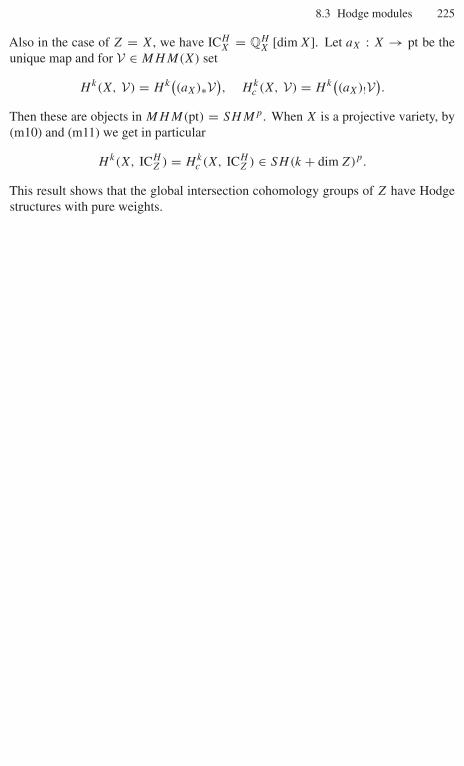
8.3 Hodge modules 225
Also in the case of Z = X, we have ICHX = QH
X [dim X]. Let aX : X → pt be theunique map and for V ∈ MHM(X) set
Hk(X, V) = Hk((aX)∗V
), Hk
c (X, V) = Hk((aX)!V
).
Then these are objects in MHM(pt) = SHMp. When X is a projective variety, by(m10) and (m11) we get in particular
Hk(X, ICHZ ) = Hk
c (X, ICHZ ) ∈ SH(k + dim Z)p.
This result shows that the global intersection cohomology groups of Z have Hodgestructures with pure weights.
Part II
Representation Theory
9
Algebraic Groups and Lie Algebras
In this chapter we summarize basic notions of algebraic groups and Lie algebras.For details we refer to other textbooks such as Humphreys [Hu1], Springer [Sp1],Humphreys [Hu2]. We do not give any proof here; however, various examples arepresented so that inexperienced readers can also follow the rest of this book.
9.1 Lie algebras and their enveloping algebras
Let k be a field. A Lie algebra g over k is a vector space over k endowed with abilinear operation (called a Lie bracket)
g × g → g ((x, y) �→ [x, y]) (9.1.1)
satisfying the following axioms (9.1.2), (9.1.3):
[x, x] = 0 (x ∈ g), (9.1.2)
[x, [y, z]] + [y, [z, x]] + [z, [x, y]] = 0 (x, y, z ∈ g). (9.1.3)
We call [•, •] the bracket product of g.For example, any vector space g with the bracket product
[x, y] = 0 (x, y ∈ g)
is a Lie algebra. We call such a Lie algebra commutative.Any associative algebra A over k can be regarded as a Lie algebra by setting
[x, y] = xy − yx (x, y ∈ A). (9.1.4)
In particular, the algebra End(V ) consisting of linear transformations of a vector spaceV is naturally a Lie algebra. We usually denote this Lie algebra by gl(V ). WhenV = kn, it is identified with the set of n × n-matrices and we write it as gln(k).
230 9 Algebraic Groups and Lie Algebras
A vector subspace h of a Lie algebra g which is closed under the bracket productof g is called a (Lie) subalgebra of g. A subalgebra of a Lie algebra is naturally a Liealgebra. The following are all subalgebras of gln(k)):
sln(k) = {x ∈ gln(k) | Tr(x) = 0}, (9.1.5)
son(k) = {x ∈ gln(k) | t x + x = 0}, (9.1.6)
sp2m(k) = {x ∈ gl2m(k) | t xJ + Jx = 0} (n = 2m), (9.1.7)
where we put
J =(
O E
−E O
)(E is the unit matrix of size m). (9.1.8)
Let g1 and g2 be Lie algebras. A linear map f : g1 → g2 preserving the bracketproducts is called a homomorphism of Lie algebras.
Let g be a Lie algebra. Then there exists uniquely up to isomorphisms a pair(A, i) of an associative algebra A and a homomorphism i : g → A of Lie algebrassatisfying the following universal property:{
For any such pair (A′, i′) there exists a unique homomorphismf : A → A′ of associative algebras such that f ◦ i = i′. (9.1.9)
We denote this associative algebra by U(g) and call it the enveloping algebra ofg. It can be realized as the quotient of the tensor algebra T (g) of g by the two-sidedideal generated by the elements xy − yx − [x, y] (x, y ∈ g). The following theoremdue to Poincaré–Birkhoff–Witt (we call it PBW for short hereafter) is fundamental inthe theory of Lie algebras.
Theorem 9.1.1. If x1, . . . , xn is a basis of the k-vector space g, then the elements
i(x1)m1 · · · i(xn)mn (m1, . . . , mn ∈ N = {0, 1, 2, . . . })
in U(g) form a basis of U(g).
It follows from PBW that i : g → U(g) is injective. Hereafter, we consider g asembedded into U(g) and omit the injection i.
Let g be a Lie algebra and let V be a vector space. We call a homomorphism
σ : g → gl(V ) (9.1.10)
of Lie algebras a representation of g on V . In this case we also say that V is a g-module.By the universal property of U(g) giving a g-module structure on a vector space V
is equivalent to giving a homomorphism U(g) → End(V ) of associative algebras.Namely, a g-module is a (left) U(g)-module, and vice versa. Universal envelopingalgebras are indispensable tools in the representation theory of Lie algebras.
9.2 Semisimple Lie algebras (1) 231
9.2 Semisimple Lie algebras (1)
From now on we assume that Lie algebras are finite dimensional unless otherwisestated. A subspace a of a Lie algebra g satisfying the condition [g, a] ⊂ a is calledan ideal of g. In this case a is clearly a Lie subalgebra of g. Moreover, the quotientspace g/a is naturally a Lie algebra.
If there exists a sequence of ideals of g:
g = a0 ⊃ a1 ⊃ a2 ⊃ · · · · · · ⊃ ar = {0}such that [ai/ai+1, ai/ai+1] = 0 (i.e., ai/ai+1 is commutative), we call g a solvableLie algebra. For a Lie algebra g there always exists a unique maximal solvable idealr(g) of g, called the radical of g. A Lie algebra g is called semisimple if r(g) = 0.For any Lie algebra g the quotient Lie algebra g/r(g) is semisimple. Moreover, it isknown that there exists a semisimple subalgebra s of g such that g = s⊕ r(g) (Levi’stheorem).
ALie algebra g is called simple if it is non-commutative and contains no non-trivialideals (ideals other than {0} and g itself). Simple Lie algebras are semisimple. If thecharacteristic of the ground field k is zero, any semisimple Lie algebra is isomorphicto a direct sum of simple Lie algebras.
For x ∈ g we define a linear map ad(x) : g → g by
(ad(x))(y) = [x, y] (y ∈ g). (9.2.1)
Thenad : g → gl(g) (9.2.2)
is a homomorphism of Lie algebras, and hence it gives a representation of g. We callit the adjoint representation of g.
We define a symmetric bilinear form Bg : g × g → k on g by
Bg(x, y) = Tr(ad(x) ad(y)) (x, y ∈ g). (9.2.3)
This is called the Killing form of g.
Theorem 9.2.1 (Cartan’s criterion). We assume that the characteristic of k is 0.Then a Lie algebra g is semisimple if and only if its Killing form Bg is non-degenerate.
By this theorem we can check the semisimplicity of the Lie algebras sln(k) (n �2), son(k) (n � 3), sp2n(k) (n � 2).
In the rest of this section we assume that k is an algebraically closed field ofcharacteristic zero and g is a semisimple Lie algebra over k.
Definition 9.2.2. We say that a subalgebra h of g is a Cartan subalgebra if it ismaximal among the subalgebras of g satisfying the following two conditions:
h is commutative. (9.2.4)
For any h ∈ h the linear transformation ad(h) is semisimple. (9.2.5)
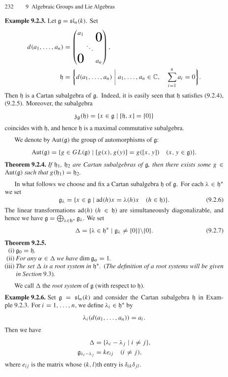
232 9 Algebraic Groups and Lie Algebras
Example 9.2.3. Let g = sln(k). Set
d(a1, . . . , an) =
⎛⎜⎜⎜⎝a1 0
. . .
0 an
⎞⎟⎟⎟⎠ ,
h ={
d(a1, . . . , an)
∣∣∣∣ a1, . . . , an ∈ C,
n∑i=1
ai = 0
}.
Then h is a Cartan subalgebra of g. Indeed, it is easily seen that h satisfies (9.2.4),(9.2.5). Moreover, the subalgebra
zg(h) = {x ∈ g | [h, x] = {0}}coincides with h, and hence h is a maximal commutative subalgebra.
We denote by Aut(g) the group of automorphisms of g:
Aut(g) = {g ∈ GL(g) | [g(x), g(y)] = g([x, y]) (x, y ∈ g)}.Theorem 9.2.4. If h1, h2 are Cartan subalgebras of g, then there exists some g ∈Aut(g) such that g(h1) = h2.
In what follows we choose and fix a Cartan subalgebra h of g. For each λ ∈ h∗we set
gλ = {x ∈ g | ad(h)x = λ(h)x (h ∈ h)}. (9.2.6)
The linear transformations ad(h) (h ∈ h) are simultaneously diagonalizable, andhence we have g = ⊕
λ∈h∗ gλ. We set
� = {λ ∈ h∗ | gλ = {0}}\{0}. (9.2.7)
Theorem 9.2.5.(i) g0 = h.
(ii) For any α ∈ � we have dim gα = 1.(iii) The set � is a root system in h∗. (The definition of a root systems will be given
in Section 9.3).
We call � the root system of g (with respect to h).
Example 9.2.6. Set g = sln(k) and consider the Cartan subalgebra h in Exam-ple 9.2.3. For i = 1, . . . , n, we define λi ∈ h∗ by
λi(d(a1, . . . , an)) = ai.
Then we have
� = {λi − λj | i = j},gλi−λj
= keij (i = j),
where eij is the matrix whose (k, l)th entry is δikδjl .
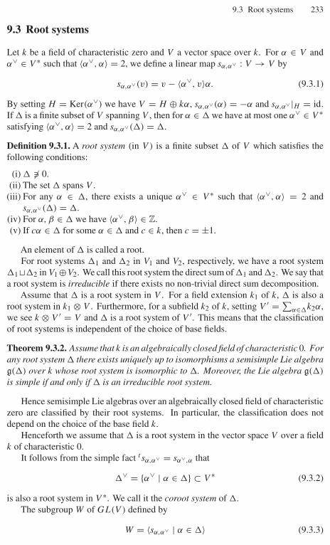
9.3 Root systems 233
9.3 Root systems
Let k be a field of characteristic zero and V a vector space over k. For α ∈ V andα∨ ∈ V ∗ such that 〈α∨, α〉 = 2, we define a linear map sα,α∨ : V → V by
sα,α∨(v) = v − 〈α∨, v〉α. (9.3.1)
By setting H = Ker(α∨) we have V = H ⊕ kα, sα,α∨(α) = −α and sα,α∨|H = id.If � is a finite subset of V spanning V , then for α ∈ � we have at most one α∨ ∈ V ∗satisfying 〈α∨, α〉 = 2 and sα,α∨(�) = �.
Definition 9.3.1. A root system (in V ) is a finite subset � of V which satisfies thefollowing conditions:
(i) � 0.(ii) The set � spans V .
(iii) For any α ∈ �, there exists a unique α∨ ∈ V ∗ such that 〈α∨, α〉 = 2 andsα,α∨(�) = �.
(iv) For α, β ∈ � we have 〈α∨, β〉 ∈ Z.(v) If cα ∈ � for some α ∈ � and c ∈ k, then c = ±1.
An element of � is called a root.For root systems �1 and �2 in V1 and V2, respectively, we have a root system
�1 ��2 in V1 ⊕V2. We call this root system the direct sum of �1 and �2. We say thata root system is irreducible if there exists no non-trivial direct sum decomposition.
Assume that � is a root system in V . For a field extension k1 of k, � is also aroot system in k1 ⊗ V . Furthermore, for a subfield k2 of k, setting V ′ = ∑
α∈�k2α,we see k ⊗ V ′ = V and � is a root system of V ′. This means that the classificationof root systems is independent of the choice of base fields.
Theorem 9.3.2. Assume that k is an algebraically closed field of characteristic 0. Forany root system � there exists uniquely up to isomorphisms a semisimple Lie algebrag(�) over k whose root system is isomorphic to �. Moreover, the Lie algebra g(�)
is simple if and only if � is an irreducible root system.
Hence semisimple Lie algebras over an algebraically closed field of characteristiczero are classified by their root systems. In particular, the classification does notdepend on the choice of the base field k.
Henceforth we assume that � is a root system in the vector space V over a fieldk of characteristic 0.
It follows from the simple fact t sα,α∨ = sα∨,α that
�∨ = {α∨ | α ∈ �} ⊂ V ∗ (9.3.2)
is also a root system in V ∗. We call it the coroot system of �.The subgroup W of GL(V ) defined by
W = 〈sα,α∨ | α ∈ �〉 (9.3.3)
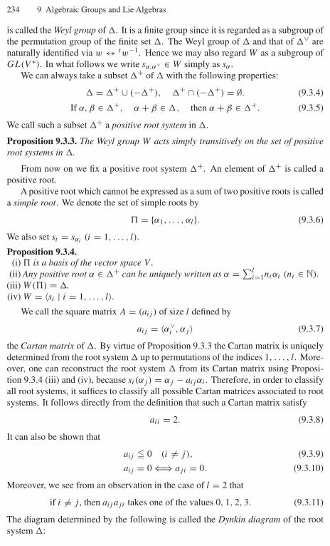
234 9 Algebraic Groups and Lie Algebras
is called the Weyl group of �. It is a finite group since it is regarded as a subgroup ofthe permutation group of the finite set �. The Weyl group of � and that of �∨ arenaturally identified via w ↔ tw−1. Hence we may also regard W as a subgroup ofGL(V ∗). In what follows we write sα,α∨ ∈ W simply as sα .
We can always take a subset �+ of � with the following properties:
� = �+ ∪ (−�+), �+ ∩ (−�+) = ∅. (9.3.4)
If α, β ∈ �+, α + β ∈ �, then α + β ∈ �+. (9.3.5)
We call such a subset �+ a positive root system in �.
Proposition 9.3.3. The Weyl group W acts simply transitively on the set of positiveroot systems in �.
From now on we fix a positive root system �+. An element of �+ is called apositive root.
A positive root which cannot be expressed as a sum of two positive roots is calleda simple root. We denote the set of simple roots by
$ = {α1, . . . , αl}. (9.3.6)
We also set si = sαi(i = 1, . . . , l).
Proposition 9.3.4.(i) $ is a basis of the vector space V .
(ii) Any positive root α ∈ �+ can be uniquely written as α = ∑li=1niαi (ni ∈ N).
(iii) W($) = �.(iv) W = 〈si | i = 1, . . . , l〉.
We call the square matrix A = (aij ) of size l defined by
aij = 〈α∨i , αj 〉 (9.3.7)
the Cartan matrix of �. By virtue of Proposition 9.3.3 the Cartan matrix is uniquelydetermined from the root system � up to permutations of the indices 1, . . . , l. More-over, one can reconstruct the root system � from its Cartan matrix using Proposi-tion 9.3.4 (iii) and (iv), because si(αj ) = αj − aij αi . Therefore, in order to classifyall root systems, it suffices to classify all possible Cartan matrices associated to rootsystems. It follows directly from the definition that such a Cartan matrix satisfy
aii = 2. (9.3.8)
It can also be shown that
aij � 0 (i = j), (9.3.9)
aij = 0 ⇐⇒ aji = 0. (9.3.10)
Moreover, we see from an observation in the case of l = 2 that
if i = j , then aij aji takes one of the values 0, 1, 2, 3. (9.3.11)
The diagram determined by the following is called the Dynkin diagram of the rootsystem �:
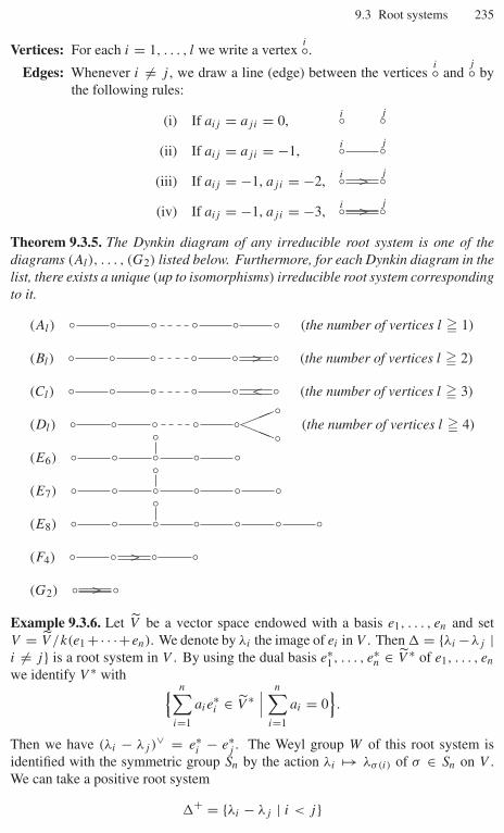
9.3 Root systems 235
Vertices: For each i = 1, . . . , l we write a vertexi◦.
Edges: Whenever i = j , we draw a line (edge) between the verticesi◦ and
j◦ bythe following rules:
(i) If aij = aji = 0, � �i j
(ii) If aij = aji = −1, � �i j
(iii) If aij = −1, aji = −2, � �>i j
(iv) If aij = −1, aji = −3, � �>i j
Theorem 9.3.5. The Dynkin diagram of any irreducible root system is one of thediagrams (Al), . . . , (G2) listed below. Furthermore, for each Dynkin diagram in thelist, there exists a unique (up to isomorphisms) irreducible root system correspondingto it.
(Al) � � � � � � (the number of vertices l � 1)
(Bl) � � � � � > � (the number of vertices l � 2)
(Cl) � � � � � < � (the number of vertices l � 3)
(Dl) � � � � � ��
���
(the number of vertices l � 4)
(E6) � � �� � �(E7) � � �� � � �(E8) � � �� � � � �(F4) � � > � �(G2) � > �
Example 9.3.6. Let V be a vector space endowed with a basis e1, . . . , en and setV = V /k(e1 +· · ·+en). We denote by λi the image of ei in V . Then � = {λi −λj |i = j} is a root system in V . By using the dual basis e∗
1, . . . , e∗n ∈ V ∗ of e1, . . . , en
we identify V ∗ with { n∑i=1
aie∗i ∈ V ∗
∣∣∣ n∑i=1
ai = 0}.
Then we have (λi − λj )∨ = e∗i − e∗
j . The Weyl group W of this root system isidentified with the symmetric group Sn by the action λi �→ λσ(i) of σ ∈ Sn on V .We can take a positive root system
�+ = {λi − λj | i < j}

236 9 Algebraic Groups and Lie Algebras
�, for which the corresponding simple root system is given by
$ = {α1, . . . , αn−1}, αi = λi − λi+1 (i = 1, 2, . . . , n − 1).
Therefore, the Dynkin diagram of � is of type (An−1).
Let us introduce several basic notation concerning root systems and Weyl groups.For i = 1, . . . , l, we define the fundamental weight πi ∈ V by the equation
〈α∨j , πi〉 = δij . (9.3.12)
We also set
Q =∑α∈�
Zα =l⊕
i=1
Zαi, (9.3.13)
Q+ =∑
α∈�+Nα =
l⊕i=1
Nαi, (9.3.14)
P = {λ ∈ V | 〈α∨, λ〉 ∈ Z (α ∈ �)} =l⊕
i=1
Zπi, (9.3.15)
P + = {λ ∈ V | 〈α∨, λ〉 ∈ N (α ∈ �+)} =l⊕
i=1
Nπi. (9.3.16)
Then Q and P are lattices (Z-lattice) in V . We call Q (resp. P ) the root lattice (resp.weight lattice).
We define a partial ordering � on V by
λ � µ ⇐⇒ λ − µ ∈ Q+. (9.3.17)
By Proposition 9.3.4 (iv) any w ∈ W can be written as
w = si1 · · · · · · sik . (9.3.18)
We denote by l(w) the minimal number k required for such expressions and call it thelength of w. The expression (9.3.18) is called a reduced expression of w if k = l(w).Let us consider two elements y, w ∈ W . If we have reduced expressions y = sj · · · sjr
and w = si1 · · · sik such that (j1, . . . , jr ) is a subsequence of (i1, . . . , ik), we writey � w. It defines a partial ordering on W called the Bruhat ordering of W . It is wellknown that there exists a unique maximal element w0 (longest element) with respectto this Bruhat ordering. It is characterized as the unique element of W with the largestlength.
9.4 Semisimple Lie algebras (2)
In this section k denotes an algebraically closed field of characteristic zero.
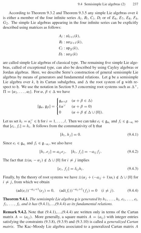
9.4 Semisimple Lie algebras (2) 237
According to Theorem 9.3.2 and Theorem 9.3.5 any simple Lie algebras over k
is either a member of the four infinite series Al , Bl , Cl , Dl or of E6, E7, E8, F4,G2. The simple Lie algebras appearing in the four infinite series can be explicitlydescribed using matrices as follows:
Al : sll+1(k),
Bl : so2l+1(k),
Cl : sp2l (k),
Dl : so2l (k)
are called simple Lie algebras of classical type. The remaining five simple Lie alge-bras, called of exceptional type, can also be described by using Cayley algebras orJordan algebras. Here, we describe Serre’s construction of general semisimple Liealgebras by means of generators and fundamental relations. Let g be a semisimpleLie algebra over k, h its Cartan subalgebra, and � the root system of g with re-spect to h. We use the notation in Section 9.3 concerning root systems such as �+,$ = {α1, . . . , αl}. For α, β ∈ � we have
[gα, gβ ] =
⎧⎪⎨⎪⎩gα+β (α + β ∈ �)
kα∨ (α + β = 0)
0 (α + β ∈ � ∪ {0}).Let us set hi = α∨
i ∈ h for i = 1, . . . , l. Then we can take ei ∈ gαiand fi ∈ g−αi
sothat [ei, fi] = hi . It follows from the commutativity of h that
[hi, hj ] = 0. (9.4.1)
Since ei ∈ gαiand fi ∈ g−αi
, we also have
[hi, ej ] = aij ej , [hi, fj ] = −aij fj . (9.4.2)
The fact that ±(αi − αj ) /∈ � ∪ {0} for i = j implies
[ei, fj ] = δij hi . (9.4.3)
Finally, by the theory of root systems we have ±(αj + (−aij + 1)αi) /∈ � ∪ {0} fori = j , from which we obtain
(ad(ei))−aij +1(ej ) = 0, (ad(fi))
−aij +1(fj ) = 0 (i = j). (9.4.4)
Theorem 9.4.1. The semisimple Lie algebra g is generated by h1, . . . , hl , e1, . . . , el ,f1, . . . , fl , and it has (9.4.1),…,(9.4.4) as its fundamental relations.
Remark 9.4.2. Note that (9.4.1),…,(9.4.4) are written only in terms of the Cartanmatrix A = (aij ). More generally, a square matrix A = (aij ) with integer entriessatisfying the constraints (9.3.8), (9.3.9) and (9.3.10) is called a generalized Cartanmatrix. The Kac–Moody Lie algebra associated to a generalized Cartan matrix A
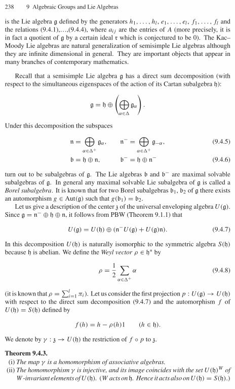
238 9 Algebraic Groups and Lie Algebras
is the Lie algebra g defined by the generators h1, . . . , hl , e1, . . . , el , f1, . . . , fl andthe relations (9.4.1),…,(9.4.4), where aij are the entries of A (more precisely, it isin fact a quotient of g by a certain ideal r which is conjectured to be 0). The Kac–Moody Lie algebras are natural generalization of semisimple Lie algebras althoughthey are infinite dimensional in general. They are important objects that appear inmany branches of contemporary mathematics.
Recall that a semisimple Lie algebra g has a direct sum decomposition (withrespect to the simultaneous eigenspaces of the action of its Cartan subalgebra h):
g = h ⊕(⊕
α∈�
gα
).
Under this decomposition the subspaces
n =⊕
α∈�+gα, n− =
⊕α∈�+
g−α, (9.4.5)
b = h ⊕ n, b− = h ⊕ n− (9.4.6)
turn out to be subalgebras of g. The Lie algebras b and b− are maximal solvablesubalgebras of g. In general any maximal solvable Lie subalgebra of g is called aBorel subalgebra. It is known that for two Borel subalgebras b1, b2 of g there existsan automorphism g ∈ Aut(g) such that g(b1) = b2.
Let us give a description of the center z of the universal enveloping algebra U(g).Since g = n− ⊕ h ⊕ n, it follows from PBW (Theorem 9.1.1) that
U(g) = U(h) ⊕ (n−U(g) + U(g)n). (9.4.7)
In this decomposition U(h) is naturally isomorphic to the symmetric algebra S(h)
because h is abelian. We define the Weyl vector ρ ∈ h∗ by
ρ = 1
2
∑α∈�+
α (9.4.8)
(it is known that ρ = ∑li=1 πi). Let us consider the first projection p : U(g) → U(h)
with respect to the direct sum decomposition (9.4.7) and the automorphism f ofU(h) = S(h) defined by
f (h) = h − ρ(h)1 (h ∈ h).
We denote by γ : z → U(h) the restriction of f ◦ p to z.
Theorem 9.4.3.(i) The map γ is a homomorphism of associative algebras.
(ii) The homomorphism γ is injective, and its image coincides with the set U(h)W ofW -invariant elements of U(h). (W acts onh. Hence it acts also on U(h) = S(h).)
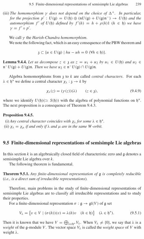
9.5 Finite-dimensional representations of semisimple Lie algebras 239
(iii) The homomorphism γ does not depend on the choice of �+. In particular,for the projection p′ : U(g) = U(h) ⊕ (nU(g) + U(g)n−) → U(h) and theautomorphism f ′ of U(h) defined by f ′(h) = h + ρ(h)1 (h ∈ h) we haveγ = f ′ ◦ p′.
We call γ the Harish-Chandra homomorphism.We note the following fact, which is an easy consequence of the PBW theorem and
z ⊂ {u ∈ U(g) | hu − uh = 0 (∀h ∈ h)}.
Lemma 9.4.4. Let us decompose z ∈ z as z = u1 + u2 by u1 ∈ U(h) and u2 ∈n−U(g) + U(g)n. Then we have u2 ∈ n−U(g) ∩ U(g)n.
Algebra homomorphisms from z to k are called central characters. For eachλ ∈ h∗ we define a central character χλ : z → k by
χλ(z) = (γ (z))(λ) (z ∈ z), (9.4.9)
where we identify U(h)(� S(h)) with the algebra of polynomial functions on h∗.The next proposition is a consequence of Theorem 9.4.3.
Proposition 9.4.5.
(i) Any central character coincides with χλ for some λ ∈ h∗.(ii) χλ = χµ if and only if λ and µ are in the same W -orbit.
9.5 Finite-dimensional representations of semisimple Lie algebras
In this section k is an algebraically closed field of characteristic zero and g denotes asemisimple Lie algebra over k.
The following theorem is fundamental.
Theorem 9.5.1. Any finite-dimensional representation of g is completely reducible(i.e., is a direct sum of irreducible representations).
Therefore, main problems in the study of finite-dimensional representations ofsemisimple Lie algebras are to classify all irreducible representations and to studytheir properties.
For a finite-dimensional representation σ : g → gl(V ) of g set
Vλ = {v ∈ V | (σ (h))(v) = λ(h)v (h ∈ h)
}(λ ∈ h∗). (9.5.1)
Then it is known that we have V = ⊕λ∈h∗Vλ. When Vλ = {0}, we say that λ is a
weight of the g-module V . The vector space Vλ is called the weight space of V withweight λ.
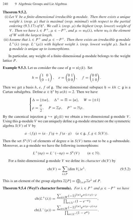
240 9 Algebraic Groups and Lie Algebras
Theorem 9.5.2.(i) Let V be a finite-dimensional irreducible g-module. Then there exists a unique
weight λ (resp. µ) that is maximal (resp. minimal) with respect to the partialordering (9.3.17) of h∗. We call λ (resp. µ) the highest (resp. lowest) weight ofV . Then we have λ ∈ P +, µ ∈ −P +, and µ = w0(λ), where w0 is the elementof W with the largest length.
(ii) Assume that λ ∈ P + and µ ∈ −P +. Then there exists an irreducible g-moduleL+(λ) (resp. L−(µ)) with highest weight λ (resp. lowest weight µ). Such ag-module is unique up to isomorphisms.
In particular, any weight of a finite-dimensional g-module belongs to the weightlattice P .
Example 9.5.3. Let us consider the case of g = sl2(k). Set
h =(
1 00 −1
), e =
(0 10 0
), f =
(0 01 0
).
Then we get a basis h, e, f of g. The one-dimensional subspace h = kh ⊂ g is aCartan subalgebra. Define α ∈ h∗ by α(h) = 2. Then we have⎧⎨⎩� = {±α}, �+ = $ = {α}, W = {±1}
ρ = α
2, P = Zρ, P + = Nρ.
By the canonical injection g ↪→ gl2(k) we obtain a two-dimensional g-module V .Using this g-module V we can uniquely define a g-module structure on the symmetricalgebra S(V ) of V by
a · (fg) = (a · f )g + f (a · g) (a ∈ g, f, g ∈ S(V )).
Then the set Sn(V ) of elements of degree n in S(V ) turns out to be a g-submodule.Moreover, as a g-module we have the following isomorphisms:
L+(nρ) = L−(−nρ) = Sn(V ) (n ∈ N).
For a finite-dimensional g-module V we define its character ch(V ) by
ch(V ) =∑λ∈P
(dim Vλ)eλ. (9.5.2)
This is an element of the group algebra Z[P ] = ⊕λ∈P Zeλ of P .
Theorem 9.5.4 (Weyl’s character formula). For λ ∈ P + and µ ∈ −P + we have
ch(L+(λ)) =∑
w∈W (−1)l(w)ew(λ+ρ)−ρ∏α∈�+(1 − e−α)
,
ch(L−(µ)) =∑
w∈W (−1)l(w)ew(µ−ρ)+ρ∏α∈�+(1 − eα)
.
9.6 Algebraic groups and their Lie algebras 241
Since L+(0) is a one-dimensional (trivial) representation of g, we have ch(L+(0))
= e0. Hence we get ∏α∈�+
(1 − e−α) =∑w∈W
(−1)l(w)ewρ−ρ (9.5.3)
(Weyl’s denominator formula) by Theorem 9.5.4.
9.6 Algebraic groups and their Lie algebras
In this section k is an algebraically closed field. If an algebraic variety G over k isendowed with a group structure and its group operations
G × G → G ((g1, g2) �→ g1g2),
G → G (g �→ g−1)
are morphisms of algebraic varieties, then we call G an algebraic group over k.For two algebraic groups G1 and G2 a morphism f : G1 → G2 of algebraic
varieties which is also a group homomorphism is called a homomorphism of algebraicgroups.
The additive group k and the multiplicative group k× of k are obviously algebraicgroups. They are denoted by Ga and Gm, respectively, when they are regarded asalgebraic groups. Abelian varieties and the general linear group
GLn(k) = {g ∈ Mn(k) | det(g) ∈ k×} (9.6.1)
= Spec k[xij , det(xij )−1]are also basic examples of algebraic groups.
It is known that an algebraic group G is affine if and only if it is isomorphic toa closed subgroup of GLn(k) for some n. In this case we call G a linear algebraicgroup. Note that Ga and Gm are linear algebraic groups by
Ga ↪→ GL2(k)
(a �→
(1 a
0 1
)), Gm � GL1(k).
In this book we are only concerned with linear algebraic groups. It is known thatany algebraic group is an extension of an abelian variety by a linear algebraic group(Chevalley–Rosenlicht’s theorem).
We can define the Lie algebra Lie(G) of an algebraic group G similarly to thecase of Lie groups as follows. For g ∈ G we define the left translation lg : G → G
and the right translation rg : G → G by lg(x) = gx and rg(x) = xg, respectively.We denote their derivations at x ∈ G by
(dlg)x : TxG → Tlg(x)G, (drg)x : TxG → Trg(x)G,
242 9 Algebraic Groups and Lie Algebras
where TxG denotes the tangent space G at x. A vector field Z on G is said to beleft-invariant (resp. right-invariant) if for any g, x ∈ G the condition
(dlg)x(Zx) = Zlg(x) (resp. (drg)x(Zx) = Zrg(x))
is satisfied. We denote the vector space of left-invariant (resp. right-invariant) vectorfields on G by Lie(G)l (resp. Lie(G)r ). These are Lie algebras by the Lie bracketoperation
[Z1, Z2](f ) = Z1(Z2(f )) − Z2(Z1(f ))
(Z1, Z2 are vector fields and f ∈ OG).
Define linear maps ϕl : Lie(G)l → TeG and ϕr : Lie(G)r → TeG by
ϕl(Z) = Ze, ϕr(Z) = Ze.
Then ϕl and ϕr are isomorphisms of vector spaces, and −ϕ−1r ◦ ϕl is an isomorphism
of Lie algebras. The Lie algebra Lie(G)l∼= Lie(G)r defined in this way is called the
Lie algebra of G and denoted by Lie(G).We will occasionally identify Lie(G) with Lie(G)l or Lie(G)r . Whenever we
use the identification of Lie(G) with invariant vector fields, we will always specifywhether the invariance is the left or right one. Identifying Te(GLn(k)) with Mn(k) =gln(k) we see that ϕl : Lie(GLn(k)) = Lie(GLn(k))l → gln(k) is an isomorphism ofLie algebras. We will identify Lie(GLn(k)) with gln(k) through ϕl in the following.In general, the Lie algebra Lie(H)l of a closed subgroup H of G is identified withthe subalgebra {Z ∈ Lie(G)l | Ze ∈ TeH } of Lie(G)l . In particular, an embeddingof G into GLn(k) gives an identification of Lie(G) as a subalgebra of gln(k). For ahomomorphism f : G1 → G2 of algebraic groups we obtain as the composite of
Lie(G1) = Lie(G1)l
ϕl−→∼ TeG1(df )e−→ TeG2
ϕl∼←− Lie(G2)l = Lie(G2)
a homomorphismdf : Lie(G1) → Lie(G2) (9.6.2)
of Lie algebras. Hence the operation Lie(•) defines a functor from the category ofalgebraic groups to that of Lie algebras. Let V be a finite-dimensional vector spaceover k. A homomorphism of algebraic groups
σ : G → GL(V ) (9.6.3)
is called a representation of G. In this case we also say that V is a G-module. Bydifferentiating σ we get a representation
dσ : Lie(G) → gl(V ) (9.6.4)
of the Lie algebra Lie(G) This defines a functor from the category of G-modules tothat of Lie(G)-modules. More generally, assume that we are given a homomorphism
9.7 Semisimple algebraic groups 243
(9.6.3) of abstract groups, where V is a (not necessarily finite-dimensional) vectorspace. Then we say that V is a G-module if there exists a family V λ (λ ∈ �) offinite-dimensional G-invariant subspaces of V satisfying the properties:
V =∑λ∈�
V λ, (9.6.5)
G → GL(V λ) is a homomorphism of algebraic groups. (9.6.6)
In this case we also have the associated Lie algebra homomorphism (9.6.4).For g ∈ G define an automorphism ig : G → G by ig(x) = gxg−1 and set
Ad(g) = dig ∈ GL(Lie(G)). (9.6.7)
ThenAd : G → GL(Lie(G)) (9.6.8)
is a representation of G. We call it the adjoint representation of G. The associatedLie algebra homomorphism
d(Ad) : Lie(G) → Lie(GL(Lie(G)))(= gl(Lie(G)))
coincides with the adjoint representation (9.2.2) of the Lie algebra Lie(G). When G
is a closed subgroup of GLn(k), the adjoint representation of G on Lie(G)(⊂ gln(k))
is described by matrices as follows:
Ad(g)x = gxg−1 (g ∈ G, x ∈ Lie(G)). (9.6.9)
9.7 Semisimple algebraic groups
In this section k is an algebraically closed field.A matrix g ∈ GLn(k) is said to be semisimple if it is diagonalizable. We also
say that g ∈ GLn(k) is unipotent if all of its eigenvalues are 1. According to thetheory of Jordan normal forms any matrix g ∈ GLn(k) can be uniquely decomposedas follows: {
g = su (s, u ∈ GLn(k))
s: semisimple, u: unipotent and su = us.(9.7.1)
This decomposition is called the Jordan decomposition.Let G be a linear algebraic group over k and fix an embedding of G into GLn(k).
It is known that in the decomposition (9.7.1) of an element g ∈ G inside the generallinear group GLn(k) we have s, u ∈ G. It is also known that the decomposition g =su does not depend on the choice of an embedding of G into a general linear group.Therefore, we can define the notions of semisimple elements, unipotent elements andJordan decompositions also for any linear algebraic group G. These notions arepreserved by homomorphisms of linear algebraic groups.
244 9 Algebraic Groups and Lie Algebras
For a linear algebraic group G there exists among all connected solvable normalclosed subgroups of G a unique maximal one R(G), called the radical of G. Theunipotent elements in R(G) form a connected normal closed subgroup Ru(G) of G,and is called the unipotent radical of G. We say that G is semisimple (resp. reductive)if R(G) = {1} (resp. Ru(G) = {1}).Example 9.7.1. The general linear group GLn(k) is reductive and its radicalR(GLn(k)) is the subgroup consisting of scalar matrices. The following closedsubgroups of GLn(k) are semisimple (except the case of n = 2 in (9.7.3)):
SLn(k) = {g ∈ GLn(k) | det(g) = 1}, (9.7.2)
SOn(k) = {g ∈ SLn(k) | t gg = 1}, (9.7.3)
Sp2m(k) = {g ∈ GL2m(k) | t gJg = J } (n = 2m), (9.7.4)
where the matrix J was defined by (9.1.8). In these cases we have Lie(SLn(k)) =sln(k), Lie(SOn(k)) = son(k) and Lie(Sp2m(k)) = sp2m(k).
A direct product of finitely many copies of the multiplicative group Gm is calleda torus. Any reductive algebraic group is “almost isomorphic to’’ a direct productof a torus and a semisimple algebraic group. Hence the essential part of the theoryof reductive algebraic groups is played by semisimple ones. It is sometimes moreconvenient to develop the theory in the framework of reductive algebraic groupsrather than just dealing with semisimple ones; however, we mainly restrict ourselvesto the case of semisimple algebraic groups in order to simplify notation.
From now on we denote by G a connected semisimple algebraic group over k andset g = Lie(G).
Maximal elements among the closed subgroups of G, which is isomorphic to atorus, is called a maximal torus of G.
Theorem 9.7.2. For two maximal tori H1 and H2 of G there exists some g ∈ G suchthat gH1g−1 = H2.
In what follows we fix a maximal torus H of G and set h = Lie(H). LetNG(H) (resp. ZG(H)) be the normalizer (resp. centralizer) of H in G. Then we haveZG(H) = H and
W = NG(H)/H (9.7.5)
turns out to be a finite group. This group W naturally acts on H . Since H is isomorphicto a direct sum of copies of Gm, the character group
L = Hom(H, k×) (9.7.6)
is a free abelian group of rank dim H . Set
LQ = Q ⊗Z L (9.7.7)
and regard L as an additive subgroup of the Q-vector space LQ. In order to avoidconfusion we denote by eλ the character of H which corresponds to λ ∈ L ⊂ LQ.
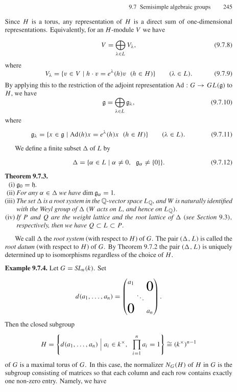
9.7 Semisimple algebraic groups 245
Since H is a torus, any representation of H is a direct sum of one-dimensionalrepresentations. Equivalently, for an H -module V we have
V =⊕λ∈L
Vλ, (9.7.8)
whereVλ = {v ∈ V | h · v = eλ(h)v (h ∈ H)} (λ ∈ L). (9.7.9)
By applying this to the restriction of the adjoint representation Ad : G → GL(g) toH , we have
g =⊕λ∈L
gλ, (9.7.10)
where
gλ = {x ∈ g | Ad(h)x = eλ(h)x (h ∈ H)} (λ ∈ L). (9.7.11)
We define a finite subset � of L by
� = {α ∈ L | α = 0, gα = {0}}. (9.7.12)
Theorem 9.7.3.(i) g0 = h.
(ii) For any α ∈ � we have dim gα = 1.(iii) The set � is a root system in the Q-vector space LQ, and W is naturally identified
with the Weyl group of � (W acts on L, and hence on LQ).
(iv) If P and Q are the weight lattice and the root lattice of � (see Section 9.3),
respectively, then we have Q ⊂ L ⊂ P .
We call � the root system (with respect to H ) of G. The pair (�, L) is called theroot datum (with respect to H ) of G. By Theorem 9.7.2 the pair (�, L) is uniquelydetermined up to isomorphisms regardless of the choice of H .
Example 9.7.4. Let G = SLn(k). Set
d(a1, . . . , an) =
⎛⎜⎜⎜⎝a1 0
. . .
0 an
⎞⎟⎟⎟⎠ .
Then the closed subgroup
H ={
d(a1, . . . , an)
∣∣∣ ai ∈ k×,
n∏i=1
ai = 1
}∼= (k×)n−1
of G is a maximal torus of G. In this case, the normalizer NG(H) of H in G is thesubgroup consisting of matrices so that each column and each row contains exactlyone non-zero entry. Namely, we have

246 9 Algebraic Groups and Lie Algebras
NG(H) ={
(aiδiσ (j))i,j=1,...,n
∣∣∣∣ σ ∈ Sn, ai ∈ k×,
(n∏
i=1
ai
)sgn(σ ) = 1
}.
Therefore, the Weyl group W = NG(H)/H is isomorphic to Sn by (aiδiσ (j))H ↔ σ .
Let us define, for i = 1, . . . , n, a character λi of H by
eλi (d(a1, . . . , an)) = ai.
Then we have an isomorphism(n⊕
i=1
Zei
) /Z
(n∑
i=1
ei
)∼←→ L =
n∑i=1
Zλi (ei ↔ λi).
We can also easily see that
� = {λi − λj | i = j}.
This is the root system of type (An−1). Moreover, L = P holds.
The action of W = Sn on H is given by
σ(d(a1, . . . , an)) = d(aσ−1(1), . . . , aσ−1(n)),
and we have
σ(λi) = λσ(i).
Example 9.7.5. In the following examples, white circles (resp. black dots �) arethe points in the root lattice Q (resp. the weight lattice P ).
(i) G = SL2(C)
� � � � � � �� � �λ2 − λ1 λ2 0 λ1
ρ = π1 α1
λ1 − λ2
� = {λ1 − λ2, λ2 − λ1} ⊃ �+ = {α1 := λ1 − λ2}=⇒ ρ = 1
2
∑α∈�+
α = 1
2α1 = π1.

9.7 Semisimple algebraic groups 247
(ii) G = SL3(C)
����������������������
���������������
����������������
� �
��
� �
�
� �
� � �
� �
�
�
�
�
� ��
�
�
� ��
�
�
�
�0
π2
π1
λ2
λ3 λ1
α2
α1
ρ
� = {λi − λj | i = j}⊃ �+ = {α1 := λ1 − λ2, α2 := λ2 − λ3, α1 + α2 = λ1 − λ3}=⇒ ρ = 1
2
∑α∈�+
α = α1 + α2 = π1 + π2.
Although Q ⊂ P , there is no inclusion relation between Q+ and P+ in this caseas we see in the following figure:
������������������
������������
������������������
������
� �
��
� �
�
�
�
�
�
��
� ��
�
�
� ��
� �� �
�
�Q+
�
�
P+
�
�
0
π2
π1
α2
α1
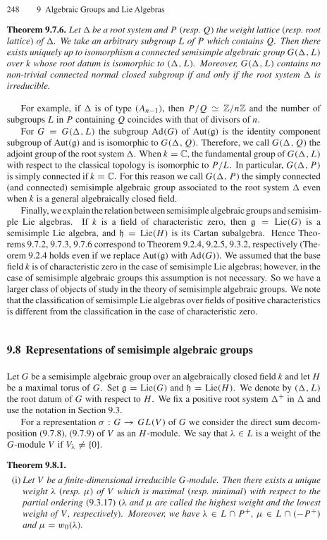
248 9 Algebraic Groups and Lie Algebras
Theorem 9.7.6. Let � be a root system and P (resp. Q) the weight lattice (resp. rootlattice) of �. We take an arbitrary subgroup L of P which contains Q. Then thereexists uniquely up to isomorphism a connected semisimple algebraic group G(�, L)
over k whose root datum is isomorphic to (�, L). Moreover, G(�, L) contains nonon-trivial connected normal closed subgroup if and only if the root system � isirreducible.
For example, if � is of type (An−1), then P/Q � Z/nZ and the number ofsubgroups L in P containing Q coincides with that of divisors of n.
For G = G(�, L) the subgroup Ad(G) of Aut(g) is the identity componentsubgroup of Aut(g) and is isomorphic to G(�, Q). Therefore, we call G(�, Q) theadjoint group of the root system �. When k = C, the fundamental group of G(�, L)
with respect to the classical topology is isomorphic to P/L. In particular, G(�, P )
is simply connected if k = C. For this reason we call G(�, P ) the simply connected(and connected) semisimple algebraic group associated to the root system � evenwhen k is a general algebraically closed field.
Finally, we explain the relation between semisimple algebraic groups and semisim-ple Lie algebras. If k is a field of characteristic zero, then g = Lie(G) is asemisimple Lie algebra, and h = Lie(H) is its Cartan subalgebra. Hence Theo-rems 9.7.2, 9.7.3, 9.7.6 correspond to Theorem 9.2.4, 9.2.5, 9.3.2, respectively (The-orem 9.2.4 holds even if we replace Aut(g) with Ad(G)). We assumed that the basefield k is of characteristic zero in the case of semisimple Lie algebras; however, in thecase of semisimple algebraic groups this assumption is not necessary. So we have alarger class of objects of study in the theory of semisimple algebraic groups. We notethat the classification of semisimple Lie algebras over fields of positive characteristicsis different from the classification in the case of characteristic zero.
9.8 Representations of semisimple algebraic groups
Let G be a semisimple algebraic group over an algebraically closed field k and let H
be a maximal torus of G. Set g = Lie(G) and h = Lie(H). We denote by (�, L)
the root datum of G with respect to H . We fix a positive root system �+ in � anduse the notation in Section 9.3.
For a representation σ : G → GL(V ) of G we consider the direct sum decom-position (9.7.8), (9.7.9) of V as an H -module. We say that λ ∈ L is a weight of theG-module V if Vλ = {0}.Theorem 9.8.1.
(i) Let V be a finite-dimensional irreducible G-module. Then there exists a uniqueweight λ (resp. µ) of V which is maximal (resp. minimal) with respect to thepartial ordering (9.3.17) (λ and µ are called the highest weight and the lowestweight of V , respectively). Moreover, we have λ ∈ L ∩ P +, µ ∈ L ∩ (−P +)
and µ = w0(λ).
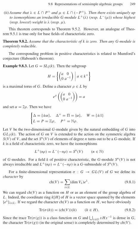
9.8 Representations of semisimple algebraic groups 249
(ii) Assume that λ ∈ L ∩ P + and µ ∈ L ∩ (−P +). Then there exists uniquely upto isomorphisms an irreducible G-module L+(λ) (resp. L−(µ)) whose highest(resp. lowest) weight is λ (resp. µ).
This theorem corresponds to Theorem 9.5.2. However, an analogue of Theo-rem 9.5.1 is true only for base fields of characteristic zero.
Theorem 9.8.2. Assume that the characteristic of k is zero. Then any G-module iscompletely reducible.
The corresponding problem in positive characteristics is related to Mumford’sconjecture (Haboush’s theorem).
Example 9.8.3. Let G = SL2(k). Then the subgroup
H ={(
a 00 a−1
) ∣∣∣∣ a ∈ k×}
is a maximal torus of G. Define a character ρ ∈ L by
eρ
((a 00 a−1
))= a
and set α = 2ρ. Then we have{� = {±α}, �+ = $ = {α}, W = {±1}L = P = Zρ, P + = Nρ.
Let V be the two-dimensional G-module given by the natural embedding of G intoGL2(k). The action of G on V is extended to the action on the symmetric algebraS(V ) of V , and the set Sn(V ) of elements of degree n turns out to be a G-module. Ifk is a field of characteristic zero, we have the isomorphisms
L+(nρ) = L−(−nρ) = Sn(V ) (n ∈ N)
of G-modules. For a field k of positive characteristic, the G-module Sn(V ) is notalways irreducible and L+(nρ) = L−(−nρ) is a G-submodule of Sn(V ).
For a finite-dimensional representation σ : G → GL(V ) of G we define itscharacter by
ch(V ) =∑λ∈L
(dim Vλ)eλ. (9.8.1)
We can regard ch(V ) as a function on H or as an element of the group algebra ofL. Indeed, the coordinate ring k[H ] of H is a vector space spanned by the elements{eλ}λ∈L. If we regard the character ch(V ) as a function on H , we have obviously
Tr(σ (h)) = (ch(V ))(h) (h ∈ H). (9.8.2)
Since the trace Tr(σ (g)) is a class function on G and⋃
x∈G xHx−1 is dense in G,the character Tr(σ (g)) (in the original sense) is completely determined by ch(V ).
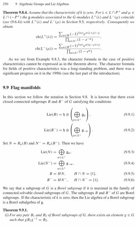
250 9 Algebraic Groups and Lie Algebras
Theorem 9.8.4. Assume that the characteristic of k is zero. For λ ∈ L∩P + and µ ∈L ∩ (−P +) the g-modules associated to the G-modules L+(λ) and L−(µ) coincide(see (9.6.4)) with L+(λ) and L−(µ) in Section 9.5, respectively. Consequently weobtain
ch(L+(λ)) =∑
w∈W (−1)l(w)ew(λ+ρ)−ρ∏α∈�+(1 − e−α)
,
ch(L−(µ)) =∑
w∈W (−1)l(w)ew(µ−ρ)+ρ∏α∈�+(1 − eα)
.
As we see from Example 9.8.3, the character formula in the case of positivecharacteristics cannot be expressed as in the theorem above. The character formulafor fields of positive characteristics was a long-standing problem, and there was asignificant progress on it in the 1990s (see the last part of the introduction).
9.9 Flag manifolds
In this section we follow the notation in Section 9.8. It is known that there existclosed connected subgroups B and B− of G satisfying the conditions
Lie(B) = h ⊕⎛⎝⊕
α∈�+gα
⎞⎠ , (9.9.1)
Lie(B−) = h ⊕⎛⎝⊕
α∈�+g−α
⎞⎠ . (9.9.2)
Set N = Ru(B) and N− = Ru(B−). Then we have
Lie(N) =⊕
α∈�+gα, (9.9.3)
Lie(N−) =⊕
α∈�+g−α, (9.9.4)
B = HN, H ∩ N = {1}, (9.9.5)
B− = HN−, H ∩ N− = {1}. (9.9.6)
We say that a subgroup of G is a Borel subgroup if it is maximal in the family ofconnected solvable closed subgroups of G. The subgroups B and B− of G are Borelsubgroups. If the characteristic of k is zero, then the Lie algebra of a Borel subgroupis a Borel subalgebra of g.
Theorem 9.9.1.(i) For any pair B1 and B2 of Borel subgroups of G, there exists an element g ∈ G
such that gB1g−1 = B2.
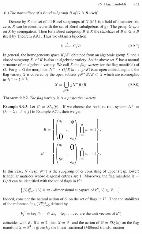
9.9 Flag manifolds 251
(ii) The normalizer of a Borel subgroup B of G is B itself.
Denote by X the set of all Borel subgroups of G (if k is a field of characteristiczero, X can be identified with the set of Borel subalgebras of g). The group G actson X by conjugation. Then for a Borel subgroup B ∈ X the stabilizer of B in G is B
itself by Theorem 9.9.1. Thus we obtain a bijection
X∼←− G/B. (9.9.7)
In general, the homogeneous space K/K ′ obtained from an algebraic group K and aclosed subgroup K ′ of K is also an algebraic variety. So the above set X has a naturalstructure of an algebraic variety. We call X the flag variety (or the flag manifold) ofG. For g ∈ G the morphism N− → G/B (n �→ gnB) is an open embedding, and theflag variety X is covered by the open subsets gN−B/B ⊂ X which are isomorphicto N− � k|�+|:
X =⋃g∈G
gN−B/B. (9.9.8)
Theorem 9.9.2. The flag variety X is a projective variety.
Example 9.9.3. Let G = SLn(k). If we choose the positive root system �+ ={λi − λj | i < j} in Example 9.7.4, then we get
B =
⎧⎪⎪⎪⎨⎪⎪⎪⎩⎛⎜⎜⎜⎝
a1 *. . .
0 an
⎞⎟⎟⎟⎠∣∣∣∣∣∣∣∣∣
n∏i=1
ai = 1
⎫⎪⎪⎪⎬⎪⎪⎪⎭ ,
B− =
⎧⎪⎪⎪⎨⎪⎪⎪⎩⎛⎜⎜⎜⎝
a1 0. . .
* an
⎞⎟⎟⎟⎠∣∣∣∣∣∣∣∣∣
n∏i=1
ai = 1
⎫⎪⎪⎪⎬⎪⎪⎪⎭ .
In this case, N (resp. N−) is the subgroup of G consisting of upper (resp. lower)triangular matrices whose diagonal entries are 1. Moreover, the flag manifold X =G/B can be identified with the set of flags in kn:{
(Vi)ni=0 | Vi is an i-dimensional subspace of kn, Vi ⊂ Vi+1
}.
Indeed, consider the natural action of G on the set of flags in kn. Then the stabilizerof the reference flag (V 0
i )ni=0 defined by
V 0i = ke1 ⊕ · · · ⊕ kei (e1, . . . , en are the unit vectors of kn)
coincides with B. If n = 2, then X = P1 and the action of G = SL2(k) on the flagmanifold X = P1 is given by the linear fractional (Möbius) transformation
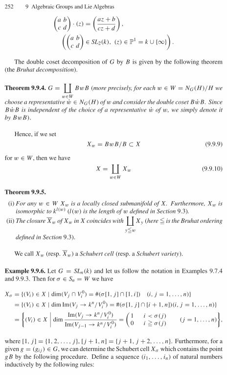
252 9 Algebraic Groups and Lie Algebras(a b
c d
)· (z) =
(az + b
cz + d
),((
a b
c d
)∈ SL2(k), (z) ∈ P1 = k ∪ {∞}
).
The double coset decomposition of G by B is given by the following theorem(the Bruhat decomposition).
Theorem 9.9.4. G =∐
w∈W
BwB (more precisely, for each w ∈ W = NG(H)/H we
choose a representative w ∈ NG(H) of w and consider the double coset BwB. SinceBwB is independent of the choice of a representative w of w, we simply denote itby BwB).
Hence, if we set
Xw = BwB/B ⊂ X (9.9.9)
for w ∈ W , then we have
X =∐
w∈W
Xw (9.9.10)
Theorem 9.9.5.
(i) For any w ∈ W Xw is a locally closed submanifold of X. Furthermore, Xw isisomorphic to kl(w) (l(w) is the length of w defined in Section 9.3).
(ii) The closure Xw of Xw in X coincides with∐y�w
Xy (here � is the Bruhat ordering
defined in Section 9.3).
We call Xw (resp. Xw) a Schubert cell (resp. a Schubert variety).
Example 9.9.6. Let G = SLn(k) and let us follow the notation in Examples 9.7.4and 9.9.3. Then for σ ∈ Sn = W we have
Xσ = {(Vi) ∈ X | dim(Vj ∩ V 0i ) = #(σ [1, j ] ∩ [1, i]) (i, j = 1, . . . , n)}
= {(Vi) ∈ X | dim Im(Vj → kn/V 0i ) = #(σ [1, j ] ∩ [i + 1, n])(i, j = 1, . . . , n)}
={
(Vi) ∈ X
∣∣∣∣ dimIm(Vj → kn/V 0
i )
Im(Vj−1 → kn/V 0i )
=(
1 i < σ(j)
0 i � σ(j)(j = 1, . . . , n)
},
where [1, j ] = {1, 2, . . . , j}, [j + 1, n] = {j + 1, j + 2, . . . , n}. Furthermore, for agiven g = (gij ) ∈ G, we can determine the Schubert cell Xσ which contains the pointgB by the following procedure. Define a sequence (i1, . . . , in) of natural numbersinductively by the following rules:

9.10 Equivariant vector bundles 253
(i) i1 is the largest number such that gi11 = 0.(ii) If the numbers i1, . . . , ir−1 are given, then ir is the largest number such that
det(gipq)p,q=1,...,r = 0.
Then we get g ∈ BσB, where σ ∈ Sn is given by σ(r) = ir .
9.10 Equivariant vector bundles
In this section G denotes any linear algebraic group over an algebraically closed fieldk. Assume that we are given an algebraic variety X over k endowed with an algebraicG-action.
Definition 9.10.1. Let V → X be an algebraic vector bundle on X. We say that V isa G-equivariant vector bundle if we are given an action of the algebraic group G onthe algebraic variety V satisfying the following condition:
For g ∈ G, x ∈ X, we have g(Vx) = Vgx, (9.10.1)
and g : Vx → Vgx is a linear isomorphism,
where Vx denotes the fiber of V at x ∈ X.
For a vector bundle V → X (of finite rank) on X denote by OX(V ) the sheafof OX-modules consisting of algebraic sections of V . Then the correspondenceV �→ OX(V ) gives an equivalence of categories:
vector bundles on X −→∼ locally free OX-modules of finite rank .
Let us interpret the notion of equivariant vector bundles in the language of OX-modules.
Notation 9.10.2.
m : G × G → G, m(g1, g2) = g1g2, (9.10.2)
σ : G × X → X, σ(g, x) = gx, (9.10.3)
p2 : G × X → X, p2(g, x) = x, (9.10.4)
p23 : G × G × X → G × X, p23(g1, g2, x) = (g2, x), (9.10.5)
f1 : G × G × X → X, f1(g1, g2, x) = x, (9.10.6)
f2 : G × G × X → X, f2(g1, g2, x) = g2x, (9.10.7)
f3 : G × G × X → X, f3(g1, g2, x) = g1g2x, (9.10.8)
Definition 9.10.3. Assume that V is a locally free OX-module of finite rank. We saythat V is G-equivariant if we are given an isomorphism
ϕ : p∗2V ∼−→ σ ∗V (9.10.9)
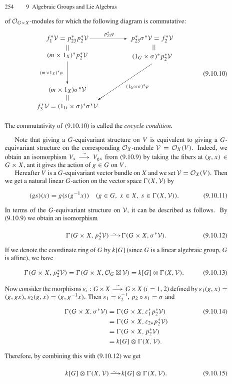
254 9 Algebraic Groups and Lie Algebras
of OG×X-modules for which the following diagram is commutative:
f ∗3 V = (1G × σ)∗σ ∗V
||(m × 1X)σ ∗V
f ∗1 V = p∗
23p∗2V
(m × 1X)∗p∗2V (1G × σ)∗p∗
2V||||
(m×1X)∗ϕ
(1G×σ)∗ϕ
p∗23ϕ
�
�
��
��
��
����
p∗23σ ∗V = f ∗
2 V
(9.10.10)
The commutativity of (9.10.10) is called the cocycle condition.
Note that giving a G-equivariant structure on V is equivalent to giving a G-equivariant structure on the corresponding OX-module V = OX(V ). Indeed, weobtain an isomorphism Vx
∼−→ Vgx from (9.10.9) by taking the fibers at (g, x) ∈G × X, ant it gives the action of g ∈ G on V .
Hereafter V is a G-equivariant vector bundle on X and we set V = OX(V ). Thenwe get a natural linear G-action on the vector space �(X, V) by
(gs)(x) = g(s(g−1x)) (g ∈ G, x ∈ X, s ∈ �(X, V)). (9.10.11)
In terms of the G-equivariant structure on V , it can be described as follows. By(9.10.9) we obtain an isomorphism
�(G × X, p∗2V) −→∼ �(G × X, σ ∗V). (9.10.12)
If we denote the coordinate ring of G by k[G] (since G is a linear algebraic group, G
is affine), we have
�(G × X, p∗2V) = �(G × X, OG � V) = k[G] ⊗ �(X, V). (9.10.13)
Now consider the morphisms εi : G×X∼−→ G×X (i = 1, 2) defined by ε1(g, x) =
(g, gx), ε2(g, x) = (g, g−1x). Then ε1 = ε−12 , p2 ◦ ε1 = σ and
�(G × X, σ ∗V) = �(G × X, ε∗1p∗
2V) (9.10.14)
= �(G × X, ε2∗p∗2V)
= �(G × X, p∗2V)
= k[G] ⊗ �(X, V).
Therefore, by combining this with (9.10.12) we get
k[G] ⊗ �(X, V) −→∼ k[G] ⊗ �(X, V). (9.10.15)
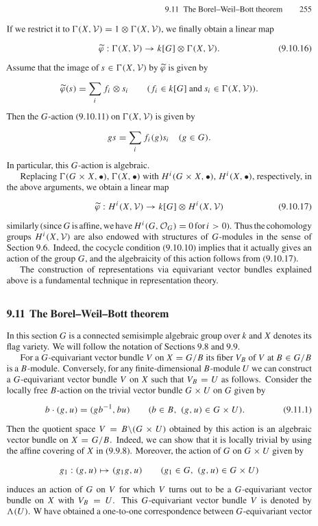
9.11 The Borel–Weil–Bott theorem 255
If we restrict it to �(X, V) = 1 ⊗ �(X, V), we finally obtain a linear map
ϕ : �(X, V) → k[G] ⊗ �(X, V). (9.10.16)
Assume that the image of s ∈ �(X, V) by ϕ is given by
ϕ(s) =∑
i
fi ⊗ si (fi ∈ k[G] and si ∈ �(X, V)).
Then the G-action (9.10.11) on �(X, V) is given by
gs =∑
i
fi(g)si (g ∈ G).
In particular, this G-action is algebraic.Replacing �(G × X, •), �(X, •) with Hi(G × X, •), Hi(X, •), respectively, in
the above arguments, we obtain a linear map
ϕ : Hi(X, V) → k[G] ⊗ Hi(X, V) (9.10.17)
similarly (since G is affine, we have Hi(G, OG) = 0 for i > 0). Thus the cohomologygroups Hi(X, V) are also endowed with structures of G-modules in the sense ofSection 9.6. Indeed, the cocycle condition (9.10.10) implies that it actually gives anaction of the group G, and the algebraicity of this action follows from (9.10.17).
The construction of representations via equivariant vector bundles explainedabove is a fundamental technique in representation theory.
9.11 The Borel–Weil–Bott theorem
In this section G is a connected semisimple algebraic group over k and X denotes itsflag variety. We will follow the notation of Sections 9.8 and 9.9.
For a G-equivariant vector bundle V on X = G/B its fiber VB of V at B ∈ G/B
is a B-module. Conversely, for any finite-dimensional B-module U we can constructa G-equivariant vector bundle V on X such that VB = U as follows. Consider thelocally free B-action on the trivial vector bundle G × U on G given by
b · (g, u) = (gb−1, bu) (b ∈ B, (g, u) ∈ G × U). (9.11.1)
Then the quotient space V = B\(G × U) obtained by this action is an algebraicvector bundle on X = G/B. Indeed, we can show that it is locally trivial by usingthe affine covering of X in (9.9.8). Moreover, the action of G on G × U given by
g1 : (g, u) �→ (g1g, u) (g1 ∈ G, (g, u) ∈ G × U)
induces an action of G on V for which V turns out to be a G-equivariant vectorbundle on X with VB = U . This G-equivariant vector bundle V is denoted by�(U). W have obtained a one-to-one correspondence between G-equivariant vector

256 9 Algebraic Groups and Lie Algebras
bundles on X and finite-dimensional B-modules. In particular, a G-equivariant linebundle on X corresponds to a one-dimensional B-module. Since the actions ofthe unipotent radical N = Ru(B) of B on one-dimensional B-modules are trivial(Jordan decompositions are preserved by homomorphisms of algebraic groups), G-equivariant line bundles on X correspond to characters λ ∈ L of H = B/N . Fora character λ ∈ L we denote the corresponding G-equivariant line bundle on X by�(λ) and set L(λ) = OX(�(λ)).
Example 9.11.1. Let G = SL2(k). Then X = P1 = k ∪ {∞} and L = P = Zρ aswe have already seen in Example 9.9.3. We can easily see that
L(nρ) = OP1(−n), (9.11.2)
where OP1(−n) is Serre’s twisted sheaf. Let us consider the two open subsets U1 = k,U2 = k× ∪ {∞} ∼= k of X and take a natural coordinate (z) (resp. x = 1/z) of U1(resp. U2). Then the line bundle �(nρ) can be obtained by gluing the two trivial linebundles U1 × k and U2 × k (on U1 and U2, respectively) by the identification
(z, u) = (x, v) ⇐⇒ x = 1
z, v = x−nu. (9.11.3)
The action of G on �(nρ) is given by(a b
c d
)· (z, u) =
(az + b
cz + d, (cz + d)nu
). (9.11.4)
Note that each cohomology group Hi(X, L(λ)) is finite dimensional because X
is a projective variety. In order to describe the G-module structure of Hi(X, L(λ))
let us introduce some notation. First set
Psing = {λ ∈ P | ∃α ∈ � such that 〈λ − ρ, α∨〉 = 0}, (9.11.5)
Preg = P \ Psing.
We define a shifted action of W on P by
w�λ = w(λ − ρ) + ρ (w ∈ W, λ ∈ P). (9.11.6)
Then W�(Psing) = Psing and we see that the anti-dominant part −P + of P is afundamental domain with respect to this shifted action (9.11.6) of W on Preg.
Theorem 9.11.2. Let λ ∈ L(⊂ P). Then we have
(i) If 〈λ, α∨〉 � 0 for any α ∈ �+ (i.e., λ ∈ −P +), then the line bundle L(λ) isgenerated by global sections. Namely, the natural morphism
OX ⊗k �(X, L(λ)) → L(λ)
is surjective.(ii) The line bundle L(λ) is ample if and only of 〈λ, α∨〉 < 0 for any α ∈ �+.
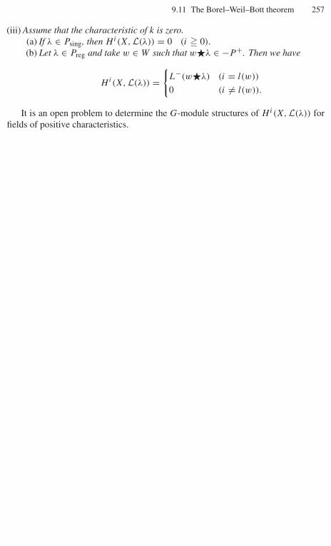
9.11 The Borel–Weil–Bott theorem 257
(iii) Assume that the characteristic of k is zero.(a) If λ ∈ Psing, then Hi(X, L(λ)) = 0 (i � 0).
(b) Let λ ∈ Preg and take w ∈ W such that w�λ ∈ −P +. Then we have
Hi(X, L(λ)) ={
L−(w�λ) (i = l(w))
0 (i = l(w)).
It is an open problem to determine the G-module structures of Hi(X, L(λ)) forfields of positive characteristics.
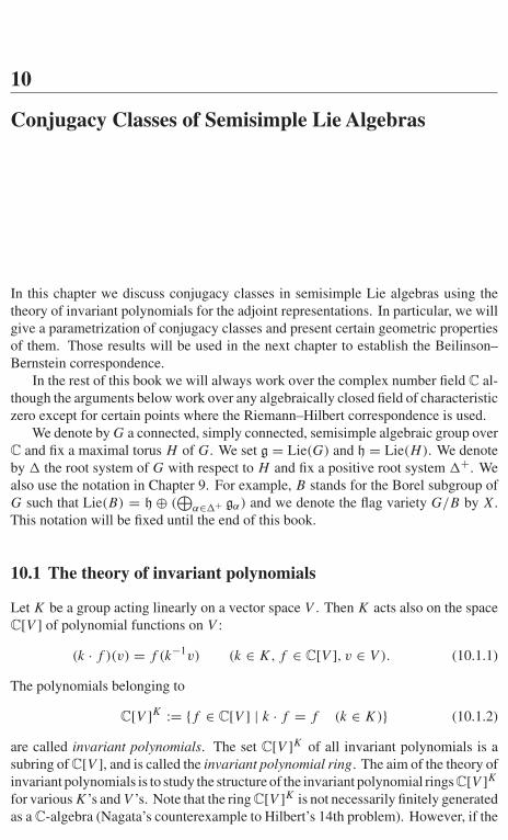
10
Conjugacy Classes of Semisimple Lie Algebras
In this chapter we discuss conjugacy classes in semisimple Lie algebras using thetheory of invariant polynomials for the adjoint representations. In particular, we willgive a parametrization of conjugacy classes and present certain geometric propertiesof them. Those results will be used in the next chapter to establish the Beilinson–Bernstein correspondence.
In the rest of this book we will always work over the complex number field C al-though the arguments below work over any algebraically closed field of characteristiczero except for certain points where the Riemann–Hilbert correspondence is used.
We denote by G a connected, simply connected, semisimple algebraic group overC and fix a maximal torus H of G. We set g = Lie(G) and h = Lie(H). We denoteby � the root system of G with respect to H and fix a positive root system �+. Wealso use the notation in Chapter 9. For example, B stands for the Borel subgroup ofG such that Lie(B) = h ⊕ (
⊕α∈�+ gα) and we denote the flag variety G/B by X.
This notation will be fixed until the end of this book.
10.1 The theory of invariant polynomials
Let K be a group acting linearly on a vector space V . Then K acts also on the spaceC[V ] of polynomial functions on V :
(k · f )(v) = f (k−1v) (k ∈ K, f ∈ C[V ], v ∈ V ). (10.1.1)
The polynomials belonging to
C[V ]K := {f ∈ C[V ] | k · f = f (k ∈ K)} (10.1.2)
are called invariant polynomials. The set C[V ]K of all invariant polynomials is asubring of C[V ], and is called the invariant polynomial ring. The aim of the theory ofinvariant polynomials is to study the structure of the invariant polynomial rings C[V ]Kfor various K’s and V ’s. Note that the ring C[V ]K is not necessarily finitely generatedas a C-algebra (Nagata’s counterexample to Hilbert’s 14th problem). However, if the
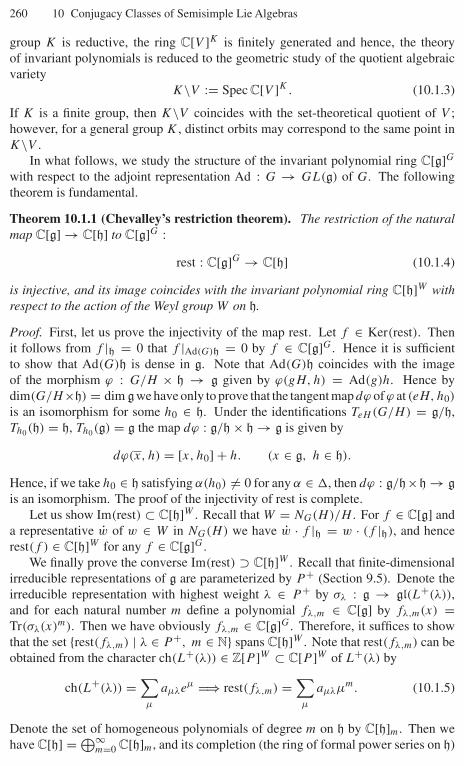
260 10 Conjugacy Classes of Semisimple Lie Algebras
group K is reductive, the ring C[V ]K is finitely generated and hence, the theoryof invariant polynomials is reduced to the geometric study of the quotient algebraicvariety
K\V := Spec C[V ]K. (10.1.3)
If K is a finite group, then K\V coincides with the set-theoretical quotient of V ;however, for a general group K , distinct orbits may correspond to the same point inK\V .
In what follows, we study the structure of the invariant polynomial ring C[g]Gwith respect to the adjoint representation Ad : G → GL(g) of G. The followingtheorem is fundamental.
Theorem 10.1.1 (Chevalley’s restriction theorem). The restriction of the naturalmap C[g] → C[h] to C[g]G :
rest : C[g]G → C[h] (10.1.4)
is injective, and its image coincides with the invariant polynomial ring C[h]W withrespect to the action of the Weyl group W on h.
Proof. First, let us prove the injectivity of the map rest. Let f ∈ Ker(rest). Thenit follows from f |h = 0 that f |Ad(G)h = 0 by f ∈ C[g]G. Hence it is sufficientto show that Ad(G)h is dense in g. Note that Ad(G)h coincides with the imageof the morphism ϕ : G/H × h → g given by ϕ(gH, h) = Ad(g)h. Hence bydim(G/H×h) = dim gwe have only to prove that the tangent map dϕ of ϕ at (eH, h0)
is an isomorphism for some h0 ∈ h. Under the identifications TeH (G/H) = g/h,Th0(h) = h, Th0(g) = g the map dϕ : g/h × h → g is given by
dϕ(x, h) = [x, h0] + h. (x ∈ g, h ∈ h).
Hence, if we take h0 ∈ h satisfying α(h0) = 0 for any α ∈ �, then dϕ : g/h×h → gis an isomorphism. The proof of the injectivity of rest is complete.
Let us show Im(rest) ⊂ C[h]W . Recall that W = NG(H)/H . For f ∈ C[g] anda representative w of w ∈ W in NG(H) we have w · f |h = w · (f |h), and hencerest(f ) ∈ C[h]W for any f ∈ C[g]G.
We finally prove the converse Im(rest) ⊃ C[h]W . Recall that finite-dimensionalirreducible representations of g are parameterized by P + (Section 9.5). Denote theirreducible representation with highest weight λ ∈ P + by σλ : g → gl(L+(λ)),and for each natural number m define a polynomial fλ,m ∈ C[g] by fλ,m(x) =Tr(σλ(x)m). Then we have obviously fλ,m ∈ C[g]G. Therefore, it suffices to showthat the set {rest(fλ,m) | λ ∈ P +, m ∈ N} spans C[h]W . Note that rest(fλ,m) can beobtained from the character ch(L+(λ)) ∈ Z[P ]W ⊂ C[P ]W of L+(λ) by
ch(L+(λ)) =∑µ
aµλeµ =⇒ rest(fλ,m) =∑µ
aµλµm. (10.1.5)
Denote the set of homogeneous polynomials of degree m on h by C[h]m. Then wehave C[h] = ⊕∞
m=0 C[h]m, and its completion (the ring of formal power series on h)
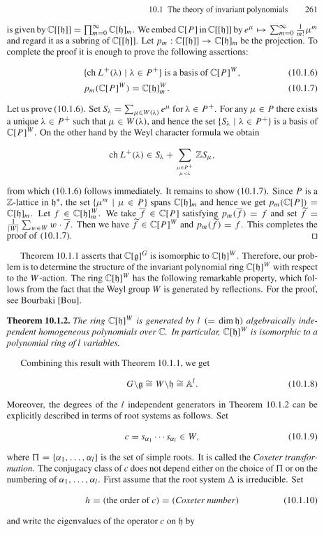
10.1 The theory of invariant polynomials 261
is given by C[[h]] = ∏∞m=0 C[h]m. We embed C[P ] in C[[h]] by eµ �→ ∑∞
m=01m!µ
m
and regard it as a subring of C[[h]]. Let pm : C[[h]] → C[h]m be the projection. Tocomplete the proof it is enough to prove the following assertions:
{ch L+(λ) | λ ∈ P +} is a basis of C[P ]W , (10.1.6)
pm(C[P ]W ) = C[h]Wm . (10.1.7)
Let us prove (10.1.6). Set Sλ = ∑µ∈W(λ) eµ for λ ∈ P +. For any µ ∈ P there exists
a unique λ ∈ P + such that µ ∈ W(λ), and hence the set {Sλ | λ ∈ P +} is a basis ofC[P ]W . On the other hand by the Weyl character formula we obtain
ch L+(λ) ∈ Sλ +∑
µ∈P+µ<λ
ZSµ,
from which (10.1.6) follows immediately. It remains to show (10.1.7). Since P is aZ-lattice in h∗, the set {µm | µ ∈ P } spans C[h]m and hence we get pm(C[P ]) =C[h]m. Let f ∈ C[h]Wm . We take f ∈ C[P ] satisfying pm(f ) = f and set f =
1|W |∑
w∈W w · f . Then we have f ∈ C[P ]W and pm(f ) = f . This completes theproof of (10.1.7). ��
Theorem 10.1.1 asserts that C[g]G is isomorphic to C[h]W . Therefore, our prob-lem is to determine the structure of the invariant polynomial ring C[h]W with respectto the W -action. The ring C[h]W has the following remarkable property, which fol-lows from the fact that the Weyl group W is generated by reflections. For the proof,see Bourbaki [Bou].
Theorem 10.1.2. The ring C[h]W is generated by l (= dim h) algebraically inde-pendent homogeneous polynomials over C. In particular, C[h]W is isomorphic to apolynomial ring of l variables.
Combining this result with Theorem 10.1.1, we get
G\g ∼= W\h ∼= Al . (10.1.8)
Moreover, the degrees of the l independent generators in Theorem 10.1.2 can beexplicitly described in terms of root systems as follows. Set
c = sα1 · · · sαl∈ W, (10.1.9)
where $ = {α1, . . . , αl} is the set of simple roots. It is called the Coxeter transfor-mation. The conjugacy class of c does not depend either on the choice of $ or on thenumbering of α1, . . . , αl . First assume that the root system � is irreducible. Set
h = (the order of c) = (Coxeter number) (10.1.10)
and write the eigenvalues of the operator c on h by

262 10 Conjugacy Classes of Semisimple Lie Algebras
exp(2π√−1m1/h), . . . , exp(2π
√−1ml/h),
(0 � m1 � m2 � · · · � ml < h).
Then it is known that
0 < m1 = 1 < m2 � · · · � ml < h, mi + ml−i+1 = h (10.1.11)l∑
i=1
mi = |�+|. (10.1.12)
We call these numbers m1, . . . , ml the exponents of the irreducible root system �. Ifthe root system � is not irreducible, the exponents of � are defined to be the union ofthose in its irreducible components (this definition is different from Bourbaki’s). Notethat the multiset of exponents of a root system � consists of l natural numbers andthe sum of all exponents is equal to the cardinality |�+| of the set of positive roots.
Theorem 10.1.3. Denote the exponents of the root system � by m1, . . . , ml . Thenthe degrees of the l algebraically independent homogeneous polynomials in Theo-rem 10.1.2 are given by m1 + 1, . . . , ml + 1.
Example 10.1.4. Let G = SLn(C), g = sln(C) and choose a Cartan subalgebra h ofg as follows:
h ={d(a1, . . . , an)
∣∣∣ n∑i=1
ai = 0},
where
d(a1, . . . , an) =
⎛⎜⎜⎜⎝a1 0
. . .
0 an
⎞⎟⎟⎟⎠ .
For i = 1, . . . , n, define λi ∈ h∗ by λi(d(a1, . . . , an)) = ai . Then C[h] =C[λ1, . . . , λn]/(λ1 + · · · + λn). Since the action of W = Sn on h is given byσ(λi) = λσ(i), C[h]W is the ring of symmetric polynomials in λ1, λ2, . . . , λn. Let usconsider the following elementary symmetric polynomials of λ1, . . . , λn:
σ1 =n∑
i=1
λi, σ2 =∑i<j
λiλj , . . . . . . , σn = λ1 · · · λn.
Then the polynomial functions σ2, . . . , σn on h are algebraically independent gener-ators of C[h]W (σ1 = 0 on h). Since the eigenvalues of the Coxeter transformation(12)(23) · · · (n − 1, n) = (1 2 3 · · · n) ∈ W = Sn are
{exp(2π
√−1k/n)}n−1
k=1 andthe Coxeter number is h = n, the exponents are 1, . . . , n − 1. This agrees withthe fact that the degrees of σ2, . . . , σn are 2, . . . , n, respectively. Now let us definepolynomial functions σk ∈ C[g] by det(t1 − x) = tn +∑n
k=1 σk(x)tn−k (x ∈ g).Then we have σk ∈ C[g]G and σ 1 = 0, rest(σ k) = σk (k = 2, . . . , n). This impliesthat σ 2, . . . , σ n are algebraically independent homogeneous generators of C[g]G.
10.2 Classification of conjugacy classes 263
10.2 Classification of conjugacy classes
The G-orbit through x ∈ g for the adjoint action of G on g is called the conjugacyclass of x. For the study of conjugacy classes, the notion of Jordan decompositionsis important. We say that x ∈ g is semisimple (resp. nilpotent) if the linear operatorad(x) ∈ gl(g) is semisimple (resp. nilpotent).
Theorem 10.2.1.(i) For any x ∈ g there exists a unique pair of elements (xs, xn) where xs is semisim-
ple and xn nilpotent, such that
x = xs + xn, [xs, xn] = 0 (10.2.1)
(We call the decomposition (10.2.1) the Jordan decomposition of x. The el-ements xs and xn are called the semisimple part and the nilpotent part of x,respectively).
(ii) Let σ : g → gl(V ) be a finite-dimensional representation of g. If x ∈ g issemisimple (resp. nilpotent), then σ(x) is semisimple (resp. nilpotent).
For the proof, see Humphreys [Hu2].A conjugacy class consisting of semisimple elements (resp. nilpotent elements)
is called a semisimple conjugacy class (resp. nilpotent conjugacy class). The classi-fication of semisimple conjugacy classes is given by the following.
Theorem 10.2.2. For any semisimple conjugacy class O the intersection O∩h with his a W -orbit in h. Hence the set of semisimple conjugacy classes in g is parameterizedby the set W\h of W -orbits in h.
Proof. Suppose that x ∈ g is a semisimple element. Then it follows directly from thedefinition of Cartan subalgebras that there exists a Cartan subalgebra h′ containing x.By the remark at the end of Section 9.7 we can take g ∈ G so that Ad(g)h′ = h. Thuswe have shown OG(x) ∩ h = ∅. Since the action of the Weyl group W on h is therestriction of the adjoint action of NG(H) = NG(h) = {g ∈ G | Ad(g)h = h} on g,OG(x)∩h is a union of W -orbits. It remains to prove that it is a single orbit. Assumethat two points h1, h2 ∈ h are conjugate in g. We will show that these two points liein the same W -orbit. By virtue of Theorem 10.1.1 h1 and h2 are mapped to the samepoint in W\h = Spec(C[h]W ). Note that W\h coincides with the set-theoreticalquotient since W is a finite group. This means that h1 and h2 are conjugate under theW -action. ��
In order to classify general conjugacy classes (which are not necessarily semisim-ple) we use Jordan decompositions. Assume that two elements x, y ∈ g are conjugate.Then their semisimple parts xs , ys are also conjugate (by the uniqueness of Jordan de-compositions). Hence we may assume that xs = ys from the beginning. Furthermore,thanks to Theorem 10.2.2, we can reduce the situation to the case of h = xs = ys ∈ h.Therefore, setting
264 10 Conjugacy Classes of Semisimple Lie Algebras
Nh = {z ∈ g | z is a nilpotent element such that [h, z] = 0}for h ∈ h, it suffices to determine when two elements h + z and h + z′ (z, z′ ∈ Nh)are conjugate to each other. If Ad(g)(h+z) = h+z′ for some g ∈ G, then it followsfrom the uniqueness of Jordan decompositions that Ad(g)h = h, i.e.,
g ∈ ZG(h) := {g ∈ G | Ad(g)h = h}.Hence we reduced the problem to the classification of orbits for the adjoint ZG(h)-action on Nh.
Theorem 10.2.3. For h ∈ h, we denote by kh the derived Lie algebra [zg(h), zg(h)]of the centralizer zg(h) = {x ∈ g | [x, h] = 0} of h. Then we have the following:
(i) The Lie algebra kh is semisimple and Nh coincides with the set of nilpotentelements in kh. In particular, we have Nh ⊂ kh.
(ii) The algebraic group ZG(h) is connected, and the orbits for the adjoint action ofZG(h) on Nh are exactly the nilpotent conjugacy classes in the semisimple Liealgebra kh.
Proof. Among connected closed subgroups H ′ of H satisfying Lie(H ′) h thereexists the smallest one S (if we regard G as a complex Lie group, S is the closure ofthe one-parameter subgroup generated by h). Then ZG(h) = ZG(S) holds. SinceS is a torus, ZG(S) is connected and reductive from a general fact on semisimplealgebraic groups. Hence if we denote the center of zg(h) = Lie(ZG(h)) by c, wehave zg(h) = c ⊕ kh and kh is a semisimple ideal of zg(h). Let z1 ∈ c, z2 ∈ kh, andset z = z1 + z2 ∈ zg(h). We see from c ⊂ h that z1 is a semisimple element of g.Suppose that the Jordan decomposition of z2 in kh is given by z2 = (z2)s + (z2)n.Then by applying Theorem 10.2.1 (ii) to the representation ad : kh → gl(g) of kh wesee that the Jordan decomposition of z in g is given by zs = z1 + (z2)s , zn = (z2)n.It follows that Nh coincides with the set of nilpotent elements in kh. Since ZG(h) isconnected, Ad(ZG(h))
∣∣kh
coincides with the adjoint group of kh. This completes theproof. ��
By Theorems 10.2.2 and 10.2.3, in order to classify conjugacy classes, it sufficesto classify nilpotent conjugacy classes. Namely, our problem is to classify G-orbitsin the nilpotent cone
N = {nilpotent elements in g} ⊂ g (10.2.2)
for an arbitrary simple Lie algebra g.Let us show that N is an irreducible closed algebraic subvariety of g. Define
fi ∈ C[g] by det(t1 − ad(x)) = tn + ∑n−1i=0 fi(x)t i . Then N is the common
zero set of f1, . . . , fn−1. In particular, it is a closed subvariety of g. Since anypoint x ∈ N is contained in a Borel subalgebra, it follows from Theorem 9.9.1 thatN = Ad(G)(b ∩ N ). Hence the irreducibility of N follows from b ∩ N = n.
To classify nilpotent conjugacy classes we need case-by-case arguments for eachsimple Lie algebra. For simple Lie algebras of classical type, we can perform the
10.2 Classification of conjugacy classes 265
classification by using linear algebra (essentially by the theory of Jordan normalforms). To treat exceptional types, some further preparation from general theories(the Jacobson–Morozov theorem) is required. The result of the classification can befound in Dynkin [Dy]. Here we only state the following general fact (It follows fromthe Dynkin–Kostant theory. The proof below is due to R. Richardson [Ri]).
Theorem 10.2.4. The number of G-orbits in N is finite.
Proof. Set G = GL(g) and g = gl(g). We regard g as a subalgebra of g by theembedding ad : g ↪→ g. Define an action of G on g by
g · x = gxg−1 (g ∈ G, x ∈ g). (10.2.3)
Then for g ∈ G, we see that the adjoint action of g on g coincides with the restrictionof the action (10.2.3) of Ad(g) ∈ G on g. Denote the set of nilpotent linear endomor-phisms of g by N . Then by the definition of N we have N = N ∩ g. On the otherhand, it follows from the theory of Jordan normal forms that the number of G-orbitsin N is finite (see Example 10.2.6). Therefore, it suffices to show that for a G-orbitO in g the intersection Z = O ∩ g with g consists of finitely many Ad(G)-orbits.
Let us consider a decreasing sequence of closed subvarieties of Z
Z = Z0 ⊃ Z1 ⊃ Z2 ⊃ · · · (10.2.4)
defined inductively by Zi = (Zi−1)sing = (the set of singular points in Zi−1). Thenevery Zi\Zi+1 is a G-invariant set, and we have to show that Zi\Zi+1 is a unionof finitely many Ad(G)-orbits. For this, it suffices to prove that every Ad(G)-orbitO = OG(x) (through x ∈ Zi\Zi+1) in Zi\Zi+1 is open. Since Zi\Zi+1 is smooth,it is enough to show the equality TxO = Tx(Zi\Zi+1) of tangent spaces. Let usconcentrate on proving the inclusion TxO ⊃ Tx(Zi\Zi+1), because the converseTxO ⊂ Tx(Zi\Zi+1) is trivial. Under the identification of Tx g with g, we havenatural isomorphisms TxO = [g, x] and Tx(Zi\Zi+1) ⊂ Tx(O) ∩ g = [g, x] ∩ g.Consequently it remains to show the following inclusion:
[g, x] ∩ g ⊂ [g, x]. (10.2.5)
Let us define a symmetric bilinear form on g by
(x1, x2) = Tr(x1x2) (x1, x2 ∈ g). (10.2.6)
It is easily checked that this bilinear form is non-degenerate. Furthermore, its re-striction to g is the Killing form, and hence it is also non-degenerate. Therefore, wehave the orthogonal decomposition g = g ⊕ g⊥, where g⊥ = {y ∈ g | (y, g) = 0}.Moreover, we have [g, g⊥] ⊂ g⊥. Indeed, for x1, x2 ∈ g, y ∈ g⊥ we have
(x1, [x2, y]) = Tr(x1x2y) − Tr(x1yx2) = Tr(x1x2y) − Tr(x2x1y)
= ([x1, x2], y) = 0.
Hence we get [g, x] ∩ g = ([g, x] + [g⊥, x]) ∩ g ⊂ [g, x] + ([g⊥, g] ∩ g) = [g, x].This completes the proof. ��
266 10 Conjugacy Classes of Semisimple Lie Algebras
The irreducibility of the nilpotent cone N implies the following result.
Corollary 10.2.5. There exists an open dense orbit in N .
Example 10.2.6. Let us consider the case of g = sln(C) and G = SLn(C). Sincethe adjoint action of G on g is given by Ad(g)x = gxg−1, there exists a bijectionbetween the set conjugacy classes of g and that of Jordan normal forms. Moreover,the Jordan decomposition of a Jordan normal form is given by writing it into a sum ofa diagonal matrix and a strictly upper triangular matrix. As a representative of eachnilpotent conjugacy class, we can choose a Jordan normal form whose eigenvaluesare all zero. Consequently, the number of nilpotent conjugacy classes is equal tothe number of the ways of writing n as a sum of natural numbers (i.e., the partitionnumber P(n) of n).
10.3 Geometry of conjugacy classes
By Theorem 10.1.1 we have C[h]W � C[g]G ⊂ C[g]. On the other hand thering C[h]W is isomorphic to the polynomial ring of l (= dim h)-variables by Theo-rem 10.1.2. Therefore, we get a natural morphism
χ : g → W\h ∼= Al (10.3.1)
of algebraic varieties. Set-theoretically this morphism χ is described as follows.
Proposition 10.3.1. Let x ∈ g. Then the image χ(x) is the point of W\h whichcorresponds to the W -orbit OG(xs) ∩ h (see Theorem 10.2.2).
Proof. Since any fiber of χ is G-invariant, we may assume that xs = h ∈ h. Underthe notation in Section 10.2, it is enough to show that the set χ(h + Nh) is just aone-point set. By Theorem 10.2.3 and Corollary 10.2.5 there is a dense ZG(h)-orbitin Nh. Hence there is also a dense ZG(h)-orbit in h + Nh. Since χ is constant oneach G-orbit, our assertion is clear. ��
The next corollary follows immediately from the proof of this proposition andCorollary 10.2.5.
Corollary 10.3.2. Every fiber of χ is irreducible and consists of finitely many con-jugacy classes. In particular, there exists an open dense conjugacy class in eachfiber.
In the rest of this section we study geometric properties of the morphism χ andits fibers. Since b is a B-module by the adjoint action, we can associate to it a vectorbundle g := �(b) → X on the flag variety X = G/B (see Section 9.11). This vectorbundle g is isomorphic to the quotient B\(G× b) of the product bundle G× b by thelocally free B-action on G × b given by
b · (g, x) = (gb−1, Ad(b)x) (b ∈ B, (g, x) ∈ G × b). (10.3.2)
10.3 Geometry of conjugacy classes 267
We define morphisms ρ : g → g and θ : g → h by
ρ((g, x)) = Ad(g)x, θ((g, x)) = p(x) (x ∈ b, g ∈ G), (10.3.3)
respectively, where p : b = h ⊕ n → h is the projection. Note that ρ is a compositeof the closed embedding g ↪→ g × X ((g, x) �→ (Ad(g)x, gB)) and the projectiong × X → g. Therefore, ρ is a proper morphism (note that X is a projective variety).Set d = dim X = |�+|.Proposition 10.3.3. χ is a flat morphism, and for any h ∈ W\h the dimension of thefiber χ−1(h) is equal to 2d .
Proof. Let us consider the fiber χ−1(h) for h ∈ h. By Proposition 10.3.1 we haveχ−1(h) = Ad(G)(h + n) = ρ(B\(G × (h + n))). Hence by dim(B\(G × (h +n))) = 2d we obtain dim χ−1(h) � 2d. On the other hand, if we take a pointh ∈ h such that α(h) = 0 for any α ∈ �, we have zg(h) = h, ZG(h) = H ,Nh = {0} and χ−1(h) = OG(h) ∼= G/H . This implies that the general fibers ofχ are 2d (= dim G/H)-dimensional. Hence, by the upper semicontinuity of thedimensions of fibers, the dimension of each fiber of χ should be 2d . The flatness ofχ follows from the fact that χ is an affine morphism such that all fibers have the samedimension. ��Corollary 10.3.4. The dimension of a conjugacy class is not greater than 2d.
We call a 2d-dimensional conjugacy class in g a regular conjugacy class, andan element of a regular conjugacy class is called a regular element. Each fiber of χ
contains a unique regular conjugacy class, and it is open dense in the fiber.For each x ∈ g we define an antisymmetric bilinear form βx on g by
βx(y, z) = (x, [y, z]) (y, z ∈ g), (10.3.4)
where (•, •) is the Killing form of g:
(y, z) = Tr(ad(y) ad(z)) (y, z ∈ g). (10.3.5)
By the relation (x, [y, z]) = ([x, y], z) and the non-degeneracy of the Killing formwe get
βx(y, g) = 0 ⇐⇒ y ∈ zg(x). (10.3.6)
Hence βx induces a non-degenerate antisymmetric bilinear form on g/zg(x). Inparticular, dim g/zg(x) is even. By g/zg(x) ∼= Tx(OG(x)) we obtain the following.
Proposition 10.3.5. Any conjugacy class is even-dimensional.
The bilinear forms βx (x ∈ g) gives a global 2-form β on g. Define a 2d-form ω
by ω = βd . Then by (10.3.6) we see that
x is a regular element ⇐⇒ ωx = 0. (10.3.7)
268 10 Conjugacy Classes of Semisimple Lie Algebras
Now take a nowhere vanishing dim g-form vg on g and consider the Hodge staroperator
∗ :2d∧
g∗ →l∧
g∗
defined by
ψ ∧ ϕ = (∗ψ, ϕ)vg
(ψ ∈
2d∧g∗, ϕ ∈
l∧g∗)
.
Here (•, •) stands for the non-degenerate symmetric bilinear form on∧l g∗ induced
by the Killing form.
Lemma 10.3.6. Let χ1, . . . , χl be homogeneous algebraically independent genera-tors of C[g]G. Then the l-form ∗ω coincides with dχ1 ∧ · · · ∧ dχl up to a non-zeroconstant multiple.
Proof. Set h′ = {h ∈ h | α(h) = 0 (α ∈ �)}. Since Ad(G)h′ = χ−1(W\h′) isdense in g, so is Ad(G)h. Note that ∗ω and dχ1 ∧ · · · ∧ dχl are G-invariant l-formson g. Therefore, it suffices to show that they coincide on h. Take a nowhere vanishingl-form vh on h. We define polynomials π1, π2 on h by
(∗ω)h = π1(h)vh, (dχ1 ∧ · · · ∧ dχl)h = π2(h)vh (h ∈ h). (10.3.8)
Then we have{both π1 and π2 are skew-invariants of W ,
namely, for any α ∈ �, we have sαπi = −πi .(10.3.9)
both π1 and π2 are homogeneous polynomials of degree d. (10.3.10)
The assertion (10.3.9) follows from the W -invariance of ∗ω|h, (dχ1∧· · ·∧dχl)|h andthe W -skew-invariance of vh. Since the coefficients of β are homogeneous of degree1 on g, those of ω, ∗ω are homogeneous of degree d . Therefore, π1 is a homogeneouspolynomial of degree d . If the degree of χi is mi + 1, the degree of the coefficientsof dχi is mi . This means that the homogeneous degree of π2 is
∑li=1 mi , which is
equal to d by (10.1.12). Hence the assertion (10.3.10) is also proved.On the other hand it is known that the space of W -skew-invariant polynomials on
h coincides with C[h]W (∏
α∈�+ α) (Bourbaki [Bou]). Hence both π1 and π2 coincidewith
∏α∈�+ α up to non-zero constant multiples. ��
Theorem 10.3.7 (Kostant).(i) χ is smooth at x ∈ g if and only if f x is a regular element of g.
(ii) Every fiber of χ is a reduced normal algebraic variety.
Proof. Note that χ : g → W\h ∼= Al is explicitly given by
χ(x) = (χ1(x), . . . , χl(x)).
10.3 Geometry of conjugacy classes 269
Therefore, the part (i) follows immediately from Lemma 10.3.6 and (10.3.7). ByProposition 10.3.3 any fiber of χ is complete intersection. Hence any fiber is reducedsince it contains a smooth point. Moreover, the codimension of the singular set ofeach fiber is at least two by Proposition 10.3.5, from which the normality of fibersfollows. ��
Theorem 10.3.7 is due to Kostant [Kos]. The proof presented here, which usesLemma 10.3.6, is due to W. Rossman.
Theorem 10.3.8. Let h ∈ h. Then the morphism
ρh : θ−1(h) → χ−1(h)
obtained by restricting ρ to θ−1(h) (the morphisms ρ and θ were defined in (10.3.3))gives a resolution of singularities of χ−1(h).
Proof. Since ρ is a proper morphism, its restriction ρh is also proper. Note thatθ−1(h) is an affine bundle on X whose fibers are isomorphic to h + n. This inparticular implies that θ−1(h) is a non-singular variety. Hence it is enough to provethe following statement by Theorem 10.3.7 (i):
If x ∈ χ−1(h) is a regular element of g, then ρ−1h (x) is a single point. (10.3.11)
We only prove it in the case where h = 0. The proof for the general case is reducedto that of this special case by the technique reducing the study of conjugacy classesto that of nilpotent conjugacy classes in smaller semisimple Lie algebras (see The-orem 10.2.3); however, the details are omitted. By χ−1(0) = N our problem is toshow that ρ−1
0 (x) is a single point for any regular nilpotent element x in g. Since ρ0is G-equivariant, it suffices to show it for just some regular nilpotent element x. Letα1, . . . , αl be the set of simple roots and set
n1 = {y ∈ n | y is a regular nilpotent element},
n2 =⎧⎨⎩∑
α∈�+yα
∣∣ yα ∈ gα, yαi= 0
⎫⎬⎭ .
Then these are open subsets of n and hence we have n1 ∩ n2 = ∅ (it is known thatn1 = n2, but we do not need it here). Hence we take x ∈ n1 ∩ n2. Since ρ−1
0 (x) ∼={gB ∈ X | Ad(g−1)x ∈ n}, it is enough to show that g ∈ B whenever g ∈ G
satisfies Ad(g)x ∈ n. Using the Bruhat decomposition, let us rewrite this g ∈ G byg = b1wb2 (b1, b2 ∈ B, w ∈ NG(H) is a representative of w ∈ W = NG(H)/H ).Then it follows from Ad(g)x ∈ n that Ad(w) Ad(b2)x ∈ n, and by the B-invarianceof n2 we obtain
Ad(w) Ad(b2)x =∑
α∈�+yw(α) ∈ n, yw(α) ∈ gw(α), yw(αi) = 0.
This implies w(αi) ∈ �+(i = 1, . . . , l) and we get w = 1 and g ∈ B. ��
270 10 Conjugacy Classes of Semisimple Lie Algebras
Since the subspace of g consisting of elements orthogonal to b (with respect to theKilling form) coincides with n, we obtain an isomorphism n ∼= (g/b)∗, from whichwe see that θ−1(0) ∼= T ∗X. On the other hand we have χ−1(0) = N . Hence weobtain a resolution of singularities ρ0 : T ∗X → N of the nilpotent cone N . It iscalled the Springer resolution of N . Now identify g with g∗ by the Killing form ofg and consider the composite of the morphisms ρ0 and N ↪→ g ∼= g∗. Then themorphism
γ : T ∗X → g∗ (10.3.12)
coincides with the moment map obtained by the G-action on the symplectic vari-ety T ∗X.
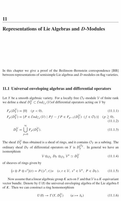
11
Representations of Lie Algebras and D-Modules
In this chapter we give a proof of the Beilinson–Bernstein correspondence [BB]between representations of semisimple Lie algebras and D-modules on flag varieties.
11.1 Universal enveloping algebras and differential operators
Let Y be a smooth algebraic variety. For a locally free OY -module V of finite rankwe define a sheaf DV
Y ⊂ EndCY(V)of differential operators acting on V by
Fp(DVY ) = {0} (p < 0), (11.1.1)
Fp(DVY ) = {P ∈ EndCY
(V) | Pf − f P ∈ Fp−1(DVY ) (f ∈ OY )} (p � 0),
(11.1.2)
DVY =
∞⋃p=0
Fp(DVY ). (11.1.3)
The sheaf DVY thus obtained is a sheaf of rings, and it contains OY as a subring. The
ordinary sheaf DY of differential operators on Y is DOY
Y . In general we have anisomorphism
V ⊗OYDY ⊗OY
V∗ � DVY (11.1.4)
of sheaves of rings given by(s ⊗ P ⊗ s∗)(t) = P(〈s∗, t〉)s (s, t ∈ V, s∗ ∈ V∗, P ∈ DY ). (11.1.5)
Now assume that a linear algebraic group K acts on Y and that V is a K-equivariantvector bundle. Denote by U(k) the universal enveloping algebra of the Lie algebra kof K . Then we can construct a ring homomorphism
U(k) → �(Y, DVY ) (a �→ ∂a) (11.1.6)

272 11 Representations of Lie Algebras and D-Modules
from U(k) to �(Y, DVY ) as follows. Let ϕ : p∗
2V −→∼ σ ∗V be the isomorphism givingthe K-equivariant structure of V , where p2 : K × Y → Y and σ : K × Y → Y arethe second projection and the action of K on Y , respectively. Then the section ∂a isuniquely determined by the condition
ϕ((a ⊗ 1) · ϕ−1(σ ∗s)) = σ ∗(∂as) (s ∈ V, a ∈ k), (11.1.7)
where a ∈ k in the left-hand side is regarded as a right-invariant vector field on K .Note that if we identify U(k) with the ring of right-invariant differential operators onK , the formula (11.1.7) holds also for any a ∈ U(k).
Remark 11.1.1. In the complex analytic category, by regarding K as a complex Liegroup we have
(∂as)(y) = d
dt(exp(ta)s((exp ta)−1y))
∣∣∣t=0
(a ∈ k, s ∈ V, y ∈ Y ).
Since �(Y, V) is a K-module, it is naturally a U(k)-module. The correspondinghomomorphism U(k) → End(�(Y, V)) coincides with the one obtained by compos-ing (11.1.6) with the homomorphism �(Y, DV
Y ) → End(�(Y, V)) induced by theinclusion DV
Y ⊂ EndCY(V).
11.2 Rings of twisted differential operators on flag varieties
Recall that for each λ ∈ P we have a G-equivariant line bundle L(λ) on the flagvariety X = G/B (see Section 9.11). We set
Dλ = DL(λ+ρ)X (λ ∈ P) (11.2.1)
(see (9.4.8) for the definition of the Weyl vector ρ). Namely, Dλ is the sheaf ofdifferential operators acting on L(λ + ρ). Since L(λ + ρ) is G-equivariant, we havea homomorphism
�λ : U(g) → �(X, Dλ) (a �→ ∂a) (11.2.2)
of associative algebras (see Section 11.1).We denote by Modqc(Dλ) the abelian category of Dλ-modules which are quasi-
coherent over OX, and by Modc(Dλ) its full subcategory consisting of coherentDλ-modules. We also denote by Mod(g) the category of U(g)-modules. By (11.2.2)we have the additive functors
Modqc(Dλ) → Mod(g) (M �→ �(X, M)), (11.2.3)
Mod(g) → Modqc(Dλ)(M �→ Dλ ⊗U(g) M
). (11.2.4)
We easily see that the functor Dλ ⊗U(g) (•) is the left adjoint functor of �(X, •).Namely, we have
HomDλ(Dλ ⊗U(g) M, N ) ∼= HomU(g)(M, �(X, N )) (11.2.5)
for any M ∈ Mod(g) and N ∈ Modqc(Dλ).
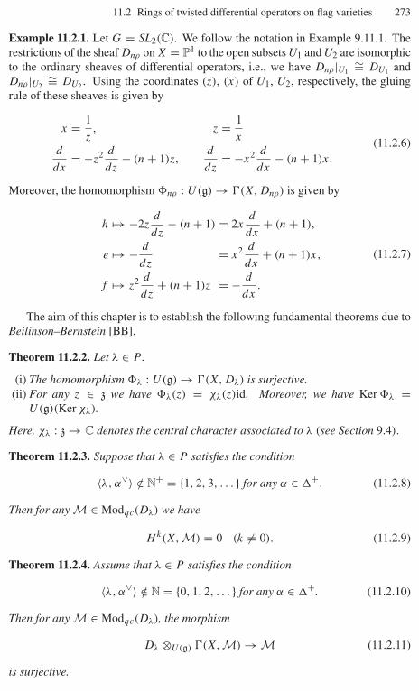
11.2 Rings of twisted differential operators on flag varieties 273
Example 11.2.1. Let G = SL2(C). We follow the notation in Example 9.11.1. Therestrictions of the sheaf Dnρ on X = P1 to the open subsets U1 and U2 are isomorphicto the ordinary sheaves of differential operators, i.e., we have Dnρ |U1
∼= DU1 andDnρ |U2
∼= DU2 . Using the coordinates (z), (x) of U1, U2, respectively, the gluingrule of these sheaves is given by
x = 1
z, z = 1
x
d
dx= −z2 d
dz− (n + 1)z,
d
dz= −x2 d
dx− (n + 1)x.
(11.2.6)
Moreover, the homomorphism �nρ : U(g) → �(X, Dnρ) is given by
h �→ −2zd
dz− (n + 1) = 2x
d
dx+ (n + 1),
e �→ − d
dz= x2 d
dx+ (n + 1)x,
f �→ z2 d
dz+ (n + 1)z = − d
dx.
(11.2.7)
The aim of this chapter is to establish the following fundamental theorems due toBeilinson–Bernstein [BB].
Theorem 11.2.2. Let λ ∈ P .
(i) The homomorphism �λ : U(g) → �(X, Dλ) is surjective.(ii) For any z ∈ z we have �λ(z) = χλ(z)id. Moreover, we have Ker �λ =
U(g)(Ker χλ).
Here, χλ : z → C denotes the central character associated to λ (see Section 9.4).
Theorem 11.2.3. Suppose that λ ∈ P satisfies the condition
〈λ, α∨〉 /∈ N+ = {1, 2, 3, . . . } for any α ∈ �+. (11.2.8)
Then for any M ∈ Modqc(Dλ) we have
Hk(X, M) = 0 (k = 0). (11.2.9)
Theorem 11.2.4. Assume that λ ∈ P satisfies the condition
〈λ, α∨〉 /∈ N = {0, 1, 2, . . . } for any α ∈ �+. (11.2.10)
Then for any M ∈ Modqc(Dλ), the morphism
Dλ ⊗U(g) �(X, M) → M (11.2.11)
is surjective.
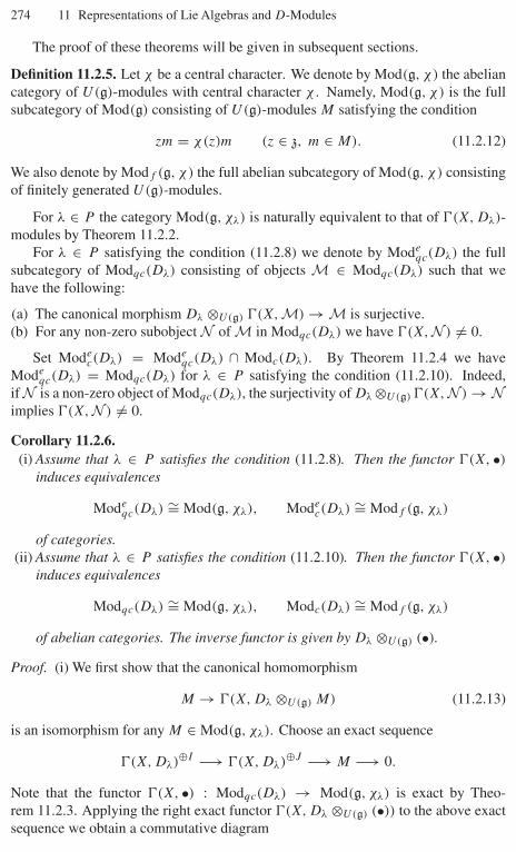
274 11 Representations of Lie Algebras and D-Modules
The proof of these theorems will be given in subsequent sections.
Definition 11.2.5. Let χ be a central character. We denote by Mod(g, χ) the abeliancategory of U(g)-modules with central character χ . Namely, Mod(g, χ) is the fullsubcategory of Mod(g) consisting of U(g)-modules M satisfying the condition
zm = χ(z)m (z ∈ z, m ∈ M). (11.2.12)
We also denote by Modf (g, χ) the full abelian subcategory of Mod(g, χ) consistingof finitely generated U(g)-modules.
For λ ∈ P the category Mod(g, χλ) is naturally equivalent to that of �(X, Dλ)-modules by Theorem 11.2.2.
For λ ∈ P satisfying the condition (11.2.8) we denote by Modeqc(Dλ) the full
subcategory of Modqc(Dλ) consisting of objects M ∈ Modqc(Dλ) such that wehave the following:
(a) The canonical morphism Dλ ⊗U(g) �(X, M) → M is surjective.(b) For any non-zero subobject N of M in Modqc(Dλ) we have �(X, N ) = 0.
Set Modec(Dλ) = Mode
qc(Dλ) ∩ Modc(Dλ). By Theorem 11.2.4 we haveMode
qc(Dλ) = Modqc(Dλ) for λ ∈ P satisfying the condition (11.2.10). Indeed,if N is a non-zero object of Modqc(Dλ), the surjectivity of Dλ ⊗U(g) �(X, N ) → Nimplies �(X, N ) = 0.
Corollary 11.2.6.(i) Assume that λ ∈ P satisfies the condition (11.2.8). Then the functor �(X, •)
induces equivalences
Modeqc(Dλ) ∼= Mod(g, χλ), Mode
c(Dλ) ∼= Modf (g, χλ)
of categories.(ii) Assume that λ ∈ P satisfies the condition (11.2.10). Then the functor �(X, •)
induces equivalences
Modqc(Dλ) ∼= Mod(g, χλ), Modc(Dλ) ∼= Modf (g, χλ)
of abelian categories. The inverse functor is given by Dλ ⊗U(g) (•).
Proof. (i) We first show that the canonical homomorphism
M → �(X, Dλ ⊗U(g) M) (11.2.13)
is an isomorphism for any M ∈ Mod(g, χλ). Choose an exact sequence
�(X, Dλ)⊕I −→ �(X, Dλ)⊕J −→ M −→ 0.
Note that the functor �(X, •) : Modqc(Dλ) → Mod(g, χλ) is exact by Theo-rem 11.2.3. Applying the right exact functor �(X, Dλ ⊗U(g) (•)) to the above exactsequence we obtain a commutative diagram
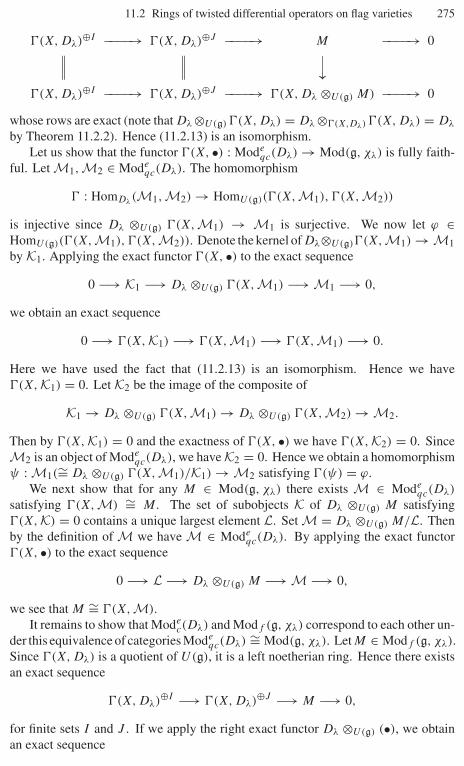
11.2 Rings of twisted differential operators on flag varieties 275
�(X, Dλ)⊕I −−−−→ �(X, Dλ)⊕J −−−−→ M −−−−→ 0∥∥∥ ∥∥∥ ⏐⏐�(X, Dλ)⊕I −−−−→ �(X, Dλ)⊕J −−−−→ �(X, Dλ ⊗U(g) M) −−−−→ 0
whose rows are exact (note that Dλ ⊗U(g) �(X, Dλ) = Dλ ⊗�(X,Dλ) �(X, Dλ) = Dλ
by Theorem 11.2.2). Hence (11.2.13) is an isomorphism.Let us show that the functor �(X, •) : Mode
qc(Dλ) → Mod(g, χλ) is fully faith-ful. Let M1, M2 ∈ Mode
qc(Dλ). The homomorphism
� : HomDλ(M1, M2) → HomU(g)(�(X, M1), �(X, M2))
is injective since Dλ ⊗U(g) �(X, M1) → M1 is surjective. We now let ϕ ∈HomU(g)(�(X, M1), �(X, M2)). Denote the kernel of Dλ⊗U(g)�(X, M1) → M1by K1. Applying the exact functor �(X, •) to the exact sequence
0 −→ K1 −→ Dλ ⊗U(g) �(X, M1) −→ M1 −→ 0,
we obtain an exact sequence
0 −→ �(X, K1) −→ �(X, M1) −→ �(X, M1) −→ 0.
Here we have used the fact that (11.2.13) is an isomorphism. Hence we have�(X, K1) = 0. Let K2 be the image of the composite of
K1 → Dλ ⊗U(g) �(X, M1) → Dλ ⊗U(g) �(X, M2) → M2.
Then by �(X, K1) = 0 and the exactness of �(X, •) we have �(X, K2) = 0. SinceM2 is an object of Mode
qc(Dλ), we have K2 = 0. Hence we obtain a homomorphismψ : M1(∼= Dλ ⊗U(g) �(X, M1)/K1) → M2 satisfying �(ψ) = ϕ.
We next show that for any M ∈ Mod(g, χλ) there exists M ∈ Modeqc(Dλ)
satisfying �(X, M) ∼= M . The set of subobjects K of Dλ ⊗U(g) M satisfying�(X, K) = 0 contains a unique largest element L. Set M = Dλ ⊗U(g) M/L. Thenby the definition of M we have M ∈ Mode
qc(Dλ). By applying the exact functor�(X, •) to the exact sequence
0 −→ L −→ Dλ ⊗U(g) M −→ M −→ 0,
we see that M ∼= �(X, M).It remains to show that Mode
c(Dλ) and Modf (g, χλ) correspond to each other un-der this equivalence of categories Mode
qc(Dλ) ∼= Mod(g, χλ). Let M ∈ Modf (g, χλ).Since �(X, Dλ) is a quotient of U(g), it is a left noetherian ring. Hence there existsan exact sequence
�(X, Dλ)⊕I −→ �(X, Dλ)⊕J −→ M −→ 0,
for finite sets I and J . If we apply the right exact functor Dλ ⊗U(g) (•), we obtainan exact sequence

276 11 Representations of Lie Algebras and D-Modules
D⊕Iλ −→ D⊕J
λ −→ Dλ ⊗U(g) M −→ 0,
and hence Dλ ⊗U(g) M is coherent. Since the object of Modeqc(Dλ) corresponding
to M is a quotient of Dλ ⊗U(g) M , it is also coherent. Let M ∈ Modec(Dλ). Since
M is coherent, it is locally generated by finitely many sections. By the surjectivityof the morphism Dλ ⊗U(g) �(X, M) → M we can take the local finite generatorsfrom �(X, M). Since X is quasi-compact, we see that M is globally generated byfinitely many elements of �(X, M). This means that we have a surjective morphismD⊕I
λ → M for a finite set I . From this we obtain a surjective homomorphism�(X, Dλ)⊕I → �(X, M), and hence �(X, M) is a finitely generated U(g)-module.
Finally, the assertion (ii) follows from Theorem 11.2.4 and (the proof of) (i). ��For any λ ∈ P there always exists w ∈ W such that w(λ) ∈ P satisfies the
condition (11.2.8),
〈w(λ), α∨〉 /∈ N+ for any α ∈ �+.
By χλ = χw(λ) (see Section 9.4) we have Mod(g, χλ) = Mod(g, χw(λ)) ∼=Mode
qc(Dw(λ)). This means that we can translate various problems in Mod(g, χλ)
into those of Modeqc(Dw(λ)).
It is also necessary in representation theory to consider problems in Mod(g, χλ)
for a general element λ ∈ h∗ = C ⊗Z P . In fact, the results in this section can beformulated in this more general situation and are known to be true. For example, letus consider the case when G = SL2(C). In Example 11.2.1 we assumed that n is aninteger. However, even if n is a general complex number, we can define the sheafDnρ by gluing the ordinary sheaves of differential operators on U1 and U2 by therule (11.2.6). Furthermore, it is also possible to define a homomorphism U(g) →�(X, Dnρ) by (11.2.7). Namely, we can also perform the constructions in (11.2.6) and(11.2.7) for general n ∈ C (the condition n ∈ Z was necessary only for the existenceof line bundles). The situation is similar for general semisimple algebraic groups G.Although there is no corresponding line bundle for a generic λ ∈ h∗ = C ⊗Z P ,we can construct a sheaf Dλ of twisted differential operators and a homomorphism�λ : U(g) → �(X, Dλ) of algebras, and then Theorems 11.2.2, 11.2.3, 11.2.4 holdwithout any modification. In this book we only treat the case where λ ∈ P for thesake of simplicity, and refer to Beilinson–Bernstein [BB] and Kashiwara [Kas14] fordetails about the general case.
11.3 Proof of Theorem 11.2.2
As in the case of DX we introduce a natural filtration {Fp(U(g))}p∈Z on U(g) by
Fp(U(g)) =
⎧⎪⎨⎪⎩0 (p < 0)
{the subspace spanned by
products of at most p elements in g} (p � 0).
(11.3.1)

11.3 Proof of Theorem 11.2.2 277
Then we have
Fp1(U(g))Fp2(U(g)) ⊂ Fp1+p2(U(g)), (11.3.2)[Fp1(U(g)), Fp2(U(g))
] ⊂ Fp1+p2−1(U(g)).
Hence if we set
grp U(g) = Fp(U(g))/Fp−1(U(g)) and gr U(g) =⊕
p
grp U(g), (11.3.3)
then gr U(g) is a commutative C-algebra. By the PBW theorem, this algebra isisomorphic to the symmetric algebra S(g) over g. Also for Dλ, set
grp Dλ = Fp(Dλ)/Fp−1(Dλ), gr Dλ =⊕
p
grp Dλ. (11.3.4)
Then gr Dλ is a sheaf of commutative OX-algebras. If we denote by π : T ∗X → X
the cotangent bundle of X, then we have a natural isomorphism gr Dλ � π∗OT ∗X.We first prove the commutative version of Theorem 11.2.2 where U(g), Dλ are
replaced by gr Dλ, gr U(g), respectively. By applying the left exact functor �(X, •)
to the exact sequence
0 −→ Fp−1(Dλ) −→ Fp(Dλ) −→ grp Dλ −→ 0, (11.3.5)
we obtain the exact sequence
0 −→ �(X, Fp−1(Dλ)) −→ �(X, Fp(Dλ)) −→ �(X, grp Dλ). (11.3.6)
Hence we have �(X, Fp(Dλ))/�(X, Fp−1(Dλ)) ⊂ �(X, grp Dλ). Therefore, by�λ(Fp(U(g))) ⊂ �(X, Fp(Dλ)) we get a homomorphism
gr �λ : S(g) = gr U(g) → �(X, gr Dλ) (11.3.7)
of C-algebras. Denote by S(g)G the set of G-invariant elements in S(g) and setS(g)G+ = S(g)G ∩ (
⊕p>0 S(g)p), where S(g)p denotes the subspace of S(g) con-
sisting of homogeneous elements of degree p � 0.
Proposition 11.3.1. The homomorphism gr �λ is surjective and its kernel Ker gr �λ
is the ideal generated by S(g)G+.
Proof. By the identifications S(g) ∼= C[g∗] = �(g∗, Og∗) and �(X, gr Dλ) ∼=�(X, p∗OT ∗X) ∼= �(T ∗X, OT ∗X), gr �λ gives a homomorphism
�(g∗, Og∗) → �(T ∗X, OT ∗X) (11.3.8)
of C-algebras. Moreover, we see by a simple calculation that this homomorphism(11.3.8) coincides with the pull-back γ ∗ of the moment map (see Section 10.3):
γ : T ∗X → g∗. (11.3.9)

278 11 Representations of Lie Algebras and D-Modules
Recall that the image of γ is the set N of nilpotent elements in g (we identify g∗ withg by the Killing form of g as in Section 10.3). Let us factorize the morphism γ as
T ∗Xγ ′�N
γ ′′↪−→ g∗.
Since γ ′ is a resolution of singularities of N and N is a normal variety, the inducedmap γ ′∗ : �(N , ON ) → �(T ∗X, OT ∗X) is an isomorphism. Furthermore, thealgebra homomorphism γ ′′∗ : �(g∗, Og∗) → �(N , ON ) is surjective because thenilpotent cone N is a closed subvariety of g∗. Hence their composite γ ∗ = γ ′∗ ◦γ ′′∗is also surjective, and its kernel is the defining ideal of N in g∗. To finish the proof,it suffices to note that this defining ideal is generated by S(g)G+ (see the proof ofTheorem 10.3.7). ��
We next study how the center z of U(g) acts on L(λ + ρ).
Proposition 11.3.2. For any z ∈ z, we have �λ(z) = χλ(z)id.
Proof. Note that for any z ∈ z = U(g)G we have �λ(z) ∈ �(X, Dλ)G. We firstprove
�(X, Dλ)G = Cid. (11.3.10)
Recall the notation in the proof of Proposition 11.3.1. Since there exists an opendense G-orbit in N (Corollary 10.2.5), we have �(N , ON )G = C. So it followsfrom the isomorphism γ ′∗ that �(X, gr Dλ)G = �(T ∗X, OT ∗X)G = C. Namely, wehave
�(X, grp Dλ)G ={
C (p = 0)
0 (p > 0).(11.3.11)
By taking the G-invariant part of (11.3.6), we get an exact sequence
0 −→ �(X, Fp−1(Dλ))G −→ �(X, Fp(Dλ))G −→ �(X, grp Dλ)G.
If p = 0, it implies �(X, F0(Dλ))G = �(X, OX)G = C (this follows also fromthe fact that X is projective). Furthermore, by induction on p we can show that�(X, Fp(Dλ))G = C for any p � 0. Hence the assertion (11.3.10) follows fromDλ = ⋃
p Fp(Dλ).It remains to show that �λ(z)s = χλ(z)s for a non-zero local section s of L(λ+ρ).
Take a non-zero element v0 in the fiber �(λ + ρ)eB of L(λ + ρ) at eB ∈ X, anddefine a section s of L(λ + ρ) on the open subset N−B/B of X by
s(uB) = uv0 (u ∈ N−). (11.3.12)
Since �(λ + ρ)eB is a B-module associated to λ + ρ, we have
�λ(h)s = (λ + ρ)(h)s (h ∈ h). (11.3.13)
It also follows from the definition of s that
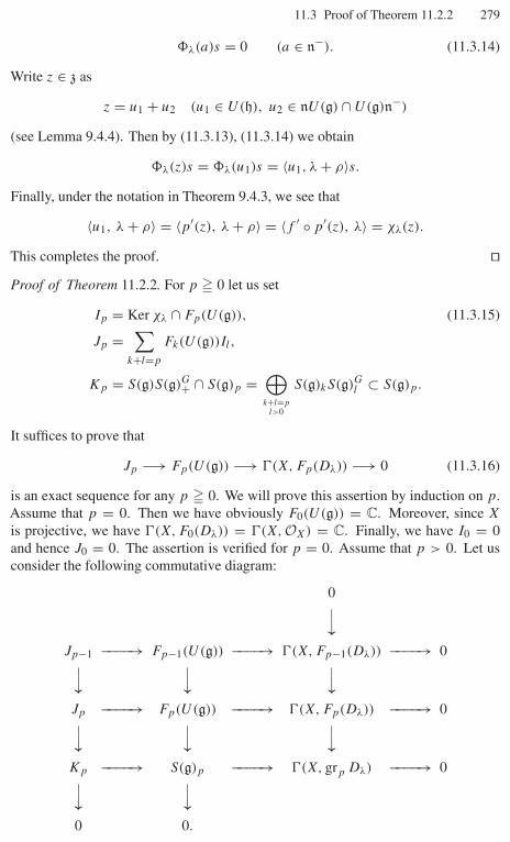
11.3 Proof of Theorem 11.2.2 279
�λ(a)s = 0 (a ∈ n−). (11.3.14)
Write z ∈ z as
z = u1 + u2 (u1 ∈ U(h), u2 ∈ nU(g) ∩ U(g)n−)
(see Lemma 9.4.4). Then by (11.3.13), (11.3.14) we obtain
�λ(z)s = �λ(u1)s = 〈u1, λ + ρ〉s.Finally, under the notation in Theorem 9.4.3, we see that
〈u1, λ + ρ〉 = 〈p′(z), λ + ρ〉 = 〈f ′ ◦ p′(z), λ〉 = χλ(z).
This completes the proof. ��Proof of Theorem 11.2.2. For p � 0 let us set
Ip = Ker χλ ∩ Fp(U(g)), (11.3.15)
Jp =∑
k+l=p
Fk(U(g))Il,
Kp = S(g)S(g)G+ ∩ S(g)p =⊕k+l=p
l>0
S(g)kS(g)Gl ⊂ S(g)p.
It suffices to prove that
Jp −→ Fp(U(g)) −→ �(X, Fp(Dλ)) −→ 0 (11.3.16)
is an exact sequence for any p � 0. We will prove this assertion by induction on p.Assume that p = 0. Then we have obviously F0(U(g)) = C. Moreover, since X
is projective, we have �(X, F0(Dλ)) = �(X, OX) = C. Finally, we have I0 = 0and hence J0 = 0. The assertion is verified for p = 0. Assume that p > 0. Let usconsider the following commutative diagram:
0⏐⏐Jp−1 −−−−→ Fp−1(U(g)) −−−−→ �(X, Fp−1(Dλ)) −−−−→ 0⏐⏐ ⏐⏐ ⏐⏐Jp −−−−→ Fp(U(g)) −−−−→ �(X, Fp(Dλ)) −−−−→ 0⏐⏐ ⏐⏐ ⏐⏐Kp −−−−→ S(g)p −−−−→ �(X, grp Dλ) −−−−→ 0⏐⏐ ⏐⏐0 0.
280 11 Representations of Lie Algebras and D-Modules
The commutativity is clear. It is also easy to see that all rows and all columns arecomplexes. The exactness of the rightmost column follows from the fact that thefunctor �(X, •) is left exact. Furthermore, the exactness of the middle column istrivial, and that of the first (resp. third) row is our hypothesis of (resp. follows fromProposition 11.3.1). Hence to prove the exactness of the middle row it is sufficient toshow that the leftmost column is exact. Note that this exactness is clear except for thesurjectivity of Jp → Kp. Hence it suffices to prove the surjectivity of Il → S(g)G
l forany l > 0. Since Fl(U(g)) → S(g)l is a surjective homomorphism of G-modules andsince all finite-dimensional G-modules are completely reducible, its G-invariant part
Fl(U(g))G = z ∩ Fl(U(g)) → S(g)Gl
is also surjective. Therefore, for any a ∈ S(g)Gl there exists z′ ∈ z ∩ Fl(U(g)) such
that σl(z′) = a (here σl : Fl(U(g)) → S(g)l is the natural map). Now let us set
z = z′ − χλ(z′)1. Then we have z ∈ Il and σl(z) = a. The surjectivity of Jp → Kp
is verified. ��
11.4 Proof of Theorems 11.2.3 and 11.2.4
For ν ∈ −P + we have a surjective morphism
pν : OX ⊗C L−(ν) � L(ν) (11.4.1)
of OX-modules by the Borel–Weil theorem. By taking its dual we get an injectivemorphism
HomOX(L(ν), OX) ↪→ OX ⊗C HomC(L−(ν), C).
By HomOX(L(ν), OX) ∼= L(−ν) and HomC(L−(ν), C) ∼= L+(−ν) we can rewrite
it asL(−ν) ↪→ OX ⊗C L+(−ν).
Applying the functor L(ν)⊗OX, we obtain an injective morphism
iν : OX ↪→ L(ν) ⊗C L+(−ν) (11.4.2)
of OX-modules.Now let λ ∈ P and let M be a Dλ-module. If we apply the functor M⊗OX
to(11.4.1) and (11.4.2), then we get morphisms
pν : M ⊗C L−(ν) → M ⊗OXL(ν), (11.4.3)
iν : M → M ⊗OXL(ν) ⊗C L+(−ν) (11.4.4)
of OX-modules. Since Ker(pν) and Im(iν) are locally direct summands of the OX-modules OX⊗CL−(ν) and L(ν)⊗CL+(−ν), respectively, the morphism pν (resp. iν)is surjective (resp. injective). The following results will be essential in our argumentsin this section.
11.4 Proof of Theorems 11.2.3 and 11.2.4 281
Proposition 11.4.1.(i) Assume that λ ∈ P satisfies the condition (11.2.10). Then Ker(pν) is a direct
summand of M ⊗C L−(ν) (globally on X) as a sheaf of abelian groups.(ii) Assume that λ ∈ P satisfies the condition (11.2.8). Then Im(iν) is a direct
summand of M ⊗OXL(ν) ⊗C L+(−ν) (globally on X) as a sheaf of abelian
groups.
Proof. In general, if M1, . . . , Mk are g-modules, then their tensor product M1 ⊗· · ·⊗Mk is also a g-module by
x · (m1 ⊗ · · · ⊗ mk) =k∑
i=1
m1 ⊗ · · · ⊗ x · mi ⊗ · · · ⊗ mk (x ∈ g and mi ∈ Mi).
Since M, L(ν), L±(∓ν) are g-modules, M ⊗OXL(ν) ⊗C L+(−ν) are also g-
modules, hence are U(g)-modules. Moreover, we easily see that (11.4.3) and (11.4.4)are homomorphisms of U(g)-modules. Decomposing these U(g)-modules by theaction of the center z of U(g), we shall show that Ker(pν) and Im(iν) are directsummands.
Note that L−(ν) has a filtration
L−(ν) = L1 ⊃ L2 ⊃ · · · ⊃ Lr−1 ⊃ Lr = {0} (11.4.5)
by B-submodules Li satisfying the following conditions (a), (b):
(a) Li/Li+1 is the irreducible B-module which corresponds to µi ∈ P . In particular,we have dim Li/Li+1 = 1.
(b) {µ1, . . . , µr−1} are the weights of L−(ν), and we have µi < µj ⇒ i < j andµi = ν ⇐⇒ i = 1.
Now consider the trivial vector bundle X × L−(ν) which corresponds to the sheafOX ⊗C L−(ν). We define a filtration
X × L−(ν) = U1 ⊃ U2 ⊃ · · · ⊃ Ur−1 ⊃ Ur (11.4.6)
of X × L−(ν) by
Ui = {(gB, l) ∈ X × L−(ν) | l ∈ g(Li)}. (11.4.7)
Denote by V i the OX-submodule of OX ⊗C L−(ν) consisting of sections of Ui . Thenthe filtration
OX ⊗C L−(ν) = V1 ⊃ V2 ⊃ · · · · · · ⊃ Vr = 0 (11.4.8)
satisfies the condition V i/V i+1 ∼= L(µi). Therefore, M ⊗C L−(ν) has a filtration
M ⊗C L−(ν) = V1 ⊃ V2 ⊃ · · · ⊃ Vr = 0 (11.4.9)
satisfying V i/V i+1 ∼= M⊗OXL(µi). Similarly, we can define a filtration of M⊗OX
L(ν) ⊗C L+(−ν)
282 11 Representations of Lie Algebras and D-Modules
M ⊗OXL(ν) ⊗C L+(−ν) = Wr ⊃ Wr−1 ⊃ · · · ⊃ W1 = 0 (11.4.10)
so that we have W i+1/W i ∼= M⊗OXL(ν −µi). Note that the preceding morphisms
pν and iν coincide with the natural morphisms V1 → V1/V2 and W2 → Wr , respec-tively. Now let us consider the action of z. Since M ⊗OX
L(µ) is a Dλ+µ-module,for any z ∈ z we have (z − χλ+µ(z))(M ⊗OX
L(µ)) = 0 by Proposition 11.3.2. So,it follows from (11.4.9) and (11.4.10) that
r−1∏i=1
(z − χλ+µi(z))(M ⊗C L−(ν)) = 0, (11.4.11)
r−1∏i=1
(z − χλ+ν−µi(z))(M ⊗OX
L(ν) ⊗C L+(−ν)) = 0, (11.4.12)
for any z ∈ z. In particular, the actions of z on M ⊗C L−(ν) and M ⊗OXL(ν) ⊗C
L+(−ν) are locally finite. In general let N be a vector space equipped with a locallyfinite z-action. For a central character χ , we set
Nχ = {n ∈ N | ∀z ∈ z, ∃p ∈ N; (z − χ(z))pn = 0}.Then, it follows from the commutativity of z that we get a direct sum decompositionN = ⊕
χ Nχ . Applying this general result to our situation, we obtain
M ⊗C L−(ν) =⊕
χ
(M ⊗C L−(ν))χ , (11.4.13)
M ⊗OXL(ν) ⊗C L+(−ν) =
⊕χ
(M ⊗OXL(ν) ⊗C L+(−ν))χ . (11.4.14)
Therefore, it remains for us to prove the following two assertions:
Under the condition (11.2.10), χλ+µi= χλ+ν implies i = 1. (11.4.15)
Under the condition (11.2.8), χλ+ν−µi= χλ implies i = 1. (11.4.16)
First we prove (11.4.15). If χλ+µi= χλ+ν , then there exists an element w ∈ W such
that w(λ + µi) = λ + ν, that is, (w(λ) − λ) + (w(µi) − ν) = 0. By (11.2.10) wehave w(λ)−λ � 0. Since w(µi) is also a weight of L−(ν), we have w(µi)− ν � 0.Consequently we obtain w(λ) − λ = w(µi) − ν = 0. By (11.2.10) and w(λ) = λ
we get w = 1 and hence µi = ν. This implies i = 1.Next we prove (11.4.16). By χλ+ν−µi
= χλ there exists an element w ∈ W suchthat w(λ) = λ+ν−µi . By (µi −ν)+(w(λ)−λ) = 0, µi −ν � 0 and w(λ)−λ � 0,we have µi = ν. This implies i = 1. ��Proof of Theorem 11.2.3. Note that Hk(X, M) = lim−→N
Hk(X, N ), where N ranges
through the family of coherent OX-submodules of M. Hence it suffices to show that

11.5 Equivariant representations and equivariant D-modules 283
Hk(X, N ) → Hk(X, M) (k = 0) is the zero map for any coherent OX-submoduleN . According to Theorem 9.11.2 (ii) there exists ν ∈ −P + such that Hk(X, N ⊗L(ν)) = 0. For such ν ∈ −P + let us consider the following commutative diagram:
Hk(X, N ) −−−−−−−−−−−−−−−−−−→ Hk(X, M)⏐⏐ ⏐⏐ (iν)∗Hk(X, N ⊗OX
L(ν) ⊗ L+(−ν))−−−−→Hk(X, M ⊗OXL(ν) ⊗ L+(−ν)).
We have Hk(X, N ⊗OXL(ν)⊗CL+(−ν)) = Hk(X, N ⊗OX
L(ν))⊗CL+(−ν) = 0.On the other hand, the map (iν)∗ is injective by Proposition 11.4.1 (ii) . HenceHk(X, N ) → Hk(X, M) is the zero map. ��Proof of Theorem 11.2.4. Denote the image of the morphism Dλ ⊗U(g) �(X, M) →M by M′ and set M′′ = M/M′. We have to show that M′′ = 0. AssumeM′′ = 0. If we take a coherent OX-submodule N = 0 of M′′, then there existsν ∈ −P + so that �(X, N ⊗OX
L(ν)) = 0 by Theorem 9.11.2 (ii). In particular, wehave �(X, M′′ ⊗OX
L(ν)) = 0. On the other hand, the map �(X, M′′ ⊗C L−(ν)) =�(X, M′′)⊗CL−(ν) → �(X, M′′⊗OX
L(ν)) is surjective by Proposition 11.4.1 (i).Therefore, we obtain �(X, M′′) = 0. Now let us consider the exact sequence
0 −→ �(X, M′) −→ �(X, M) −→ �(X, M′′) −→ 0,
(the exactness follows from Theorem 11.2.3). Note that there exists an isomorphism
�(X, M′) −→∼ �(X, M) by the definition of M′. Hence we get �(X, M′′) = 0.This is a contradiction. Thus we must have M′′ = 0. ��
11.5 Equivariant representations and equivariant D-modules
The g-modules which can be lifted to representations of a certain large subgroup K
of G are especially important in representation theory. Such g-modules are calledK-equivariant g-modules, or simply (g, K)-modules. As a large subgroup K of G,we mainly consider the following two cases:
K = B (a Borel subgroup). (11.5.1){K = Gθ = {g ∈ G | θ(g) = g},where θ is an involution of G.
(11.5.2)
We will treat the case (11.5.1) in Chapter 12. The case (11.5.2) is closely related tothe study of admissible representations of real semisimple Lie groups. The precisedefinition of K-equivariant g-modules is as follows.
Definition 11.5.1. Let K be a closed subgroup of G and set k = Lie(K). We say thata (not necessarily finite-dimensional) vector space M over C is a K-equivariant g-module, if it has both a g-module structure and a K-module structure (see Section 9.6)satisfying the following conditions:
284 11 Representations of Lie Algebras and D-Modules{The action of k on M obtained by differentiating that of K
coincides with the restriction of the g-action.(11.5.3)
k · (a · m) = ((Ad(k))(a) · (k · m) (k ∈ K, a ∈ g, m ∈ M). (11.5.4)
We denote the category of K-equivariant g-modules by Mod(g, K). Moreover,Mod(g, χ, K) (resp. Modf (g, χ, K)) stands for its full subcategory consisting ofobjects of which also belong to Mod(g, χ) (resp. Modf (g, χ)) as g-modules.
From now on, we introduce D-modules which correspond to K-equivariant g-modules. Assume that an algebraic group K is acting on a smooth algebraic varietyY . We define morphisms p2 : K × Y → Y , σ : K × Y → Y , m : K × K → K
by p2(k, y) = y, σ(k, y) = ky, m(k1, k2) = k1k2, respectively. Just by imitating thedefinition of K-equivariant locally free OY -modules in Chapter 9, we can define thenotion of K-equivariant D-modules as follows.
Definition 11.5.2. Let M be a DY -module. Suppose that we are given an isomor-phism
ϕ : p∗2M ∼−→ σ ∗M (11.5.5)
of DK×Y -modules satisfying the cocycle condition. Then we we say that M isa K-equivariant DY -module. Here the cocycle condition is the commutativity ofthe diagram obtained by replacing V with M in (9.10.10). We denote the abeliancategory of OY -quasi-coherent (resp. DY -coherent) and K-equivariant DY -modulesby Modqc(DY , K) (resp. Modc(DY , K)).
By D−ρ = DX we have Mod(g, χ−ρ) ∼= Modqc(DX) and Modf (g, χ−ρ) ∼=Modc(DX) by Corollary 11.2.6.
Theorem 11.5.3. For any closed subgroup K of G, we have Mod(g, χ−ρ, K) ∼=Modqc(DX, K) and Modf (g, χ−ρ, K) ∼= Modc(DX, K).
Proof. Since K is an affine variety, it is D-affine in the sense that the categoryModqc(DK) is equivalent to that of �(K, DK)-modules (see Proposition 1.4.3).Moreover, we have also proved that the flag variety X of G is D-affine (see Corol-lary 11.2.6). The arguments used to prove the D-affinity of X can also be appliedto K × X as well and we conclude that K × X is D-affine. Namely, the cate-gory Modqc(DK×X) is equivalent to the category of �(K × X, DK×X)-modules.As a result, giving an isomorphism ϕ : p∗
2M → σ ∗M of DK×X-modules forM ∈ Modqc(DX) is equivalent to giving an isomorphism
ϕ : �(K × X, p∗2M) → �(K × X, σ ∗M) (11.5.6)
of �(K × X, DK×X)-modules. Note that we have
�(K × X, p∗2M) ∼= �(K × X, OK � M) (11.5.7)
∼= �(K, OK) ⊗ �(X, M).
11.5 Equivariant representations and equivariant D-modules 285
On the other hand, if we define morphisms εi : K × X → K × X (i = 1, 2) byε1(k, x) = (k, kx), ε2(k, x) = (k, k−1x), then it follows from ε1 = ε−1
2 , p2 ◦ ε1 =σ that
�(K × X, σ ∗M) ∼= �(K × X, ε∗1p∗
2M) ∼= �(K × X, (ε2)∗p∗2M) (11.5.8)
∼= �(K × X, p∗2M) ∼= �(K, OK) ⊗ �(X, M).
Therefore, both �(K×X, p∗2M) and �(K×X, σ ∗M) are isomorphic to �(K, OK)⊗
�(X, M) as vector spaces. To distinguish the two actions of �(K × X, DK×X)
on �(K, OK) ⊗ �(X, M) defined by (11.5.7) and (11.5.8), we denote the ac-tion through the isomorphism (11.5.7) by (ξ, n) �→ ξ • n, and the one throughthe isomorphism (11.5.8) by (ξ, n) �→ ξ � n (where ξ ∈ �(K × X, DK×X),n ∈ �(K, OK) ⊗ �(X, M)). We give descriptions of these actions in the following.
Note that we have
�(K × X, DK×X) ∼= �(K × X, DK � DX) = �(K, DK) ⊗ �(X, DX)
and�(K, DK) ∼= �(K, OK) ⊗C U(k),
where k = Lie(K) is identified with the set of left invariant vector fields on K . Inparticular, �(K, DX) is generated by �(K, OK) and k. Moreover, it follows fromTheorem 11.2.2 that �(X, DX) ∼= U(g)/U(g) Ker χ−ρ . In particular, �(X, DX) isgenerated by the vector fields p = �−ρ(p) on X corresponding to p ∈ g. Nownote that an element h ⊗ m in �(K, OK) ⊗ �(X, M) corresponds to the sectionh ◦ p1 ⊗ p−1
2 m of p∗2M = OK×X ⊗
p−12 OX
p−12 M (resp. the section h ◦ p1 ⊗ σ−1m
of σ ∗M = OK×X⊗σ−1OXσ−1M) through the isomorphism (11.5.7) (resp. (11.5.8)),
where p1 : K×X → K is the first projection. Then it follows from these observationsand simple computations that⎧⎪⎨⎪⎩
(f ⊗ 1) • (h ⊗ m) = f h ⊗ m (f ∈ �(K, OK)),
(a ⊗ 1) • (h ⊗ m) = a · h ⊗ m (a ∈ k),
(1 ⊗ p) • (h ⊗ m) = h ⊗ p · m (p ∈ g),
(11.5.9)
⎧⎪⎨⎪⎩(f ⊗ 1) � (h ⊗ m) = f h ⊗ m (f ∈ �(K, OK)),
(a ⊗ 1) � (h ⊗ m) = a · h ⊗ m − (1 ⊗ a) � (h ⊗ m) (a ∈ k) ,
(1 ⊗ p) � (h ⊗ m) = ∑i hhi ⊗ pi · m (p ∈ g),
(11.5.10)
where we set Ad(k)p = ∑i hi(k)pi (k ∈ K , hi ∈ �(K, OK), pi ∈ g). Since the
two actions of �(K, OK) ⊗ 1 are the same as we see in the formula above, the mapϕ is uniquely determined by its restriction
ϕ : �(X, M) → �(K, OK) ⊗ �(X, M) (11.5.11)
to �(X, M) = 1 ⊗ �(X, M). From this map we obtain a morphism
τ : K × �(X, M) → �(X, M) (11.5.12)
286 11 Representations of Lie Algebras and D-Modules
defined by
ϕ(m) =∑
i
hi ⊗ mi =⇒ τ(k, m) =∑
i
hi(k)mi. (11.5.13)
Hence giving a homomorphism (11.5.6) of �(K, OK)-modules is equivalent to givingan algebraic morphism (11.5.12) satisfying the condition
τ(k, m) is linear with respect to m ∈ �(X, M). (11.5.14)
Furthermore, the cocycle condition for ϕ is equivalent to the condition
τ(k1, τ (k2, m)) = τ(k1k2, m) (k1, k2 ∈ K, m ∈ �(X, M)). (11.5.15)
Therefore, giving an isomorphism (11.5.6) of �(K, OK)-modules such that the corre-sponding morphism ϕ : p∗
2M → σ ∗M satisfies the cocycle condition is equivalentto giving a K-module structure on �(X, M) (k · m = τ(k, m)). Finally, by using(11.5.9), (11.5.10) we can easily check that the conditions for ϕ to preserve the actionsof k ⊗ 1, 1 ⊗ g correspond, respectively, to (11.5.3), (11.5.4). This completes theproof. ��Remark 11.5.4. We can also define for general λ the notion of K-equivariant Dλ-modules. Moreover, if λ satisfies the condition (11.2.10) we have an equivalenceof categories Mod(g, χλ, K) ∼= Modqc(Dλ, K) (see [Kas14]). However, in order topresent such general results we need to define an action of K on Dλ, by which thearguments become more complicated. In order to avoid it we only treat in this bookthe special case where λ = −ρ.
11.6 Classification of equivariant D-modules
When a subgroup K of G is either (11.5.1) or (11.5.2), there exist only finitely manyK-orbits on X (in the case (11.5.1) it is a consequence of Theorem 9.9.4, and in thecase (11.5.2) this is a result of T. Matsuki [Mat]). This is one way of saying that K issufficiently “large.’’ In such cases the following remarkable results hold.
Theorem 11.6.1. Let Y be a smooth algebraic variety and K an algebraic groupacting on Y . Suppose that there exist only finitely many K-orbits on Y . Denote thecategory of K-equivariant regular holonomic DY -modules by Modrh(DY , K). Wedenote also by ϒ(K, Y ) the set of pairs (O, L) of a K-orbit O ⊂ Y and an irreducibleK-equivariant local system L on Oan (the notion of K-equivariant local systems canbe defined in the same way as in the case of equivariant D-modules. We call anirreducible object in the category of K-equivariant local systems an irreducible K-equivariant local system). Then we have the following:
(i) Modc(DY , K) = Modrh(DY , K). That is, the regular holonomicity of a coherentDY -module follows from the K-equivariance.
11.6 Classification of equivariant D-modules 287
(ii) The irreducible objects in Modc(DY , K) are parameterized by the set ϒ(K, Y ).
Proof. (i) We first consider the case when Y consists of a single K-orbit, i.e., the casewhen Y = K/K ′ for a subgroup K ′ of K . Denoting the one-point algebraic varietyby pt = {x0} we define morphisms
σ : K × Y → Y, p2 : K × Y → Y, i : K → K × Y,
π : K → Y, j : pt → Y, l : K → pt
by σ(k1, k2K ′) = k1k2K ′, p2(k1, k2K ′) = k2K ′, i(k) = (k−1, kK ′), π(k) = kK ′,j (x0) = K ′, l(k) = x0, respectively. Then for any M ∈ Modc(DY , K) we have
π∗M = (p2 ◦ i)∗M = i∗p∗2M ∼= i∗σ ∗M = (σ ◦ i)∗M
= (j ◦ l)∗M = l∗j∗M = OK ⊗C (j∗M)x0 ,
and it follows from the coherence of π∗M that dim(j∗M)x0 < ∞. This implies thatπ∗M ∼= OK ⊗C (j∗M)x0 is a regular holonomic D-module. Since π is smooth, Mitself is also regular holonomic.
The general case can be proved by induction on the number of K-orbits. LetM ∈ Modc(DY , K). Take a closed K-orbit O in Y , set Y ′ = Y\O and consider theinjections i : O ↪→ Y , j : Y ′ ↪→ Y . Then we have a distinguished triangle∫
i
i†M −→ M −→∫
j
j†M +1−→ .
By our inductive assumption, (the cohomology sheaves of) j†M and i†M are regularholonomic. Hence (the cohomology sheaves of)
∫j
j†M and∫
ii†M are as well. This
implies that M is also regular holonomic.(ii) By the Riemann–Hilbert correspondence the category Modrh(DY , K) is
equivalent to the category Perv(CY , K) of K-equivariant perverse sheaves on Y an.The irreducible objects of Perv(CY , K) are parameterized by the set ϒ(K, Y ), wherea pair (O, L) ∈ ϒ(K, Y ) corresponds to the intersection cohomology complexICY (L). ��Remark 11.6.2. Let O = K/K ′ be a K-orbit. Then the category of K-equivariantlocal systems on Oan is equivalent to that of finite-dimensional representations ofK ′/(K ′)0 (here (K ′)0 is the identity component subgroup of K ′). In particular, thereexists a one-to-one correspondence between irreducible K-equivariant local systemson Oan and irreducible representations of the finite group K ′/(K ′)0.
By Theorem 11.5.3 and 11.6.1 we obtain the following result.
Corollary 11.6.3. Let K be a closed subgroup of G for which there exist only finitelymany K-orbits on the flag variety X of G. Then the irreducible K-equivariant g-modules with the central character χ−ρ are parameterized by the set ϒ(K, X).
Although we stated our results only in the case where the central character is χ−ρ ,we can argue similarly also in the general case to get a geometric classification ofirreducible K-equivariant g-modules. When K is of type (11.5.2), we thus obtain aclassification of irreducible admissible representations of real semisimple Lie groups.This gives a new approach to the Langlands classification.

12
Character Formula of Highest Weight Modules
In this chapter we will give an account of the famous character formula for irreduciblehighest weight modules over semisimple Lie algebras (the Kazhdan–Lusztig conjec-ture, a theorem due to Brylinski–Kashiwara and Beilinson–Bernstein). It became astarting point of various applications of D-module theory to representation theory.
12.1 Highest weight modules
Let M be a (not necessarily finite-dimensional) h-module. For each µ ∈ h∗ we set
Mµ = {m ∈ M | hm = µ(h)m (h ∈ h)} (12.1.1)
and call it the weight space of M with weight µ. When Mµ = {0}, we say that µ is aweight of M and the elements of Mµ are called weight vectors with weight µ. If anh-module M satisfies the conditions
M =⊕µ∈h∗
Mµ, (12.1.2)
dim Mµ < ∞ (µ ∈ h∗), (12.1.3)
then we call M a weight module and define its character by the formal infinite sum
ch(M) =∑µ∈h∗
(dim Mµ)eµ. (12.1.4)
Definition 12.1.1. Let λ ∈ h∗, and let M be a g-module. If there is an element m = 0of M such that
m ∈ Mλ, nm = {0}, U(g)m = M, (12.1.5)
we say that M is a highest weight module with highest weight λ. In this case m iscalled a highest weight vector of M .
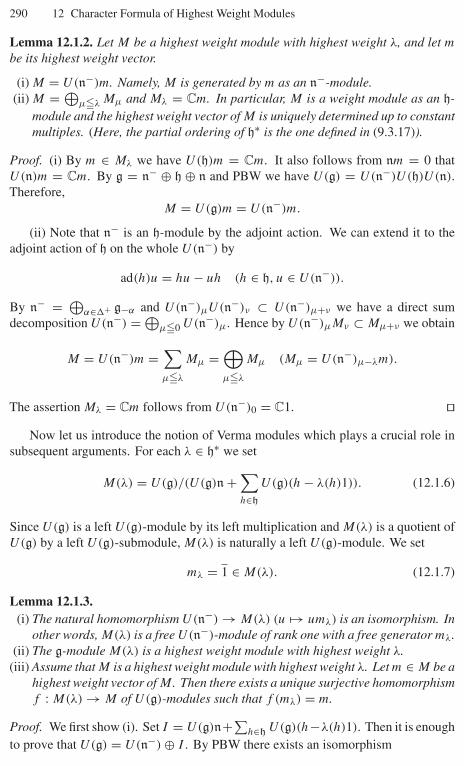
290 12 Character Formula of Highest Weight Modules
Lemma 12.1.2. Let M be a highest weight module with highest weight λ, and let m
be its highest weight vector.
(i) M = U(n−)m. Namely, M is generated by m as an n−-module.(ii) M = ⊕
µ�λ Mµ and Mλ = Cm. In particular, M is a weight module as an h-module and the highest weight vector of M is uniquely determined up to constantmultiples. (Here, the partial ordering of h∗ is the one defined in (9.3.17)).
Proof. (i) By m ∈ Mλ we have U(h)m = Cm. It also follows from nm = 0 thatU(n)m = Cm. By g = n− ⊕ h ⊕ n and PBW we have U(g) = U(n−)U(h)U(n).Therefore,
M = U(g)m = U(n−)m.
(ii) Note that n− is an h-module by the adjoint action. We can extend it to theadjoint action of h on the whole U(n−) by
ad(h)u = hu − uh (h ∈ h, u ∈ U(n−)).
By n− = ⊕α∈�+ g−α and U(n−)µU(n−)ν ⊂ U(n−)µ+ν we have a direct sum
decomposition U(n−) = ⊕µ�0 U(n−)µ. Hence by U(n−)µMν ⊂ Mµ+ν we obtain
M = U(n−)m =∑µ�λ
Mµ =⊕µ�λ
Mµ (Mµ = U(n−)µ−λm).
The assertion Mλ = Cm follows from U(n−)0 = C1. ��Now let us introduce the notion of Verma modules which plays a crucial role in
subsequent arguments. For each λ ∈ h∗ we set
M(λ) = U(g)/(U(g)n +∑h∈h
U(g)(h − λ(h)1)). (12.1.6)
Since U(g) is a left U(g)-module by its left multiplication and M(λ) is a quotient ofU(g) by a left U(g)-submodule, M(λ) is naturally a left U(g)-module. We set
mλ = 1 ∈ M(λ). (12.1.7)
Lemma 12.1.3.(i) The natural homomorphism U(n−) → M(λ) (u �→ umλ) is an isomorphism. In
other words, M(λ) is a free U(n−)-module of rank one with a free generator mλ.(ii) The g-module M(λ) is a highest weight module with highest weight λ.
(iii) Assume that M is a highest weight module with highest weight λ. Let m ∈ M be ahighest weight vector of M . Then there exists a unique surjective homomorphismf : M(λ) → M of U(g)-modules such that f (mλ) = m.
Proof. We first show (i). Set I = U(g)n+∑h∈h U(g)(h−λ(h)1). Then it is enoughto prove that U(g) = U(n−) ⊕ I . By PBW there exists an isomorphism
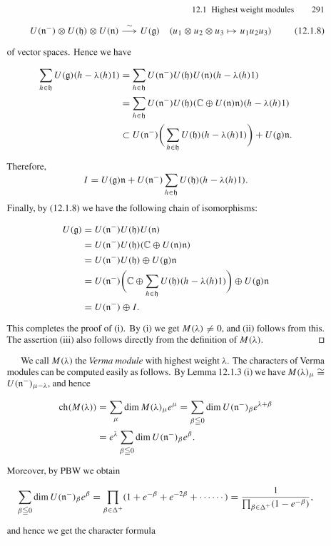
12.1 Highest weight modules 291
U(n−) ⊗ U(h) ⊗ U(n)∼−→ U(g) (u1 ⊗ u2 ⊗ u3 �→ u1u2u3) (12.1.8)
of vector spaces. Hence we have∑h∈h
U(g)(h − λ(h)1) =∑h∈h
U(n−)U(h)U(n)(h − λ(h)1)
=∑h∈h
U(n−)U(h)(C ⊕ U(n)n)(h − λ(h)1)
⊂ U(n−)
(∑h∈h
U(h)(h − λ(h)1)
)+ U(g)n.
Therefore,
I = U(g)n + U(n−)∑h∈h
U(h)(h − λ(h)1).
Finally, by (12.1.8) we have the following chain of isomorphisms:
U(g) = U(n−)U(h)U(n)
= U(n−)U(h)(C ⊕ U(n)n)
= U(n−)U(h) ⊕ U(g)n
= U(n−)
(C ⊕
∑h∈h
U(h)(h − λ(h)1)
)⊕ U(g)n
= U(n−) ⊕ I.
This completes the proof of (i). By (i) we get M(λ) = 0, and (ii) follows from this.The assertion (iii) also follows directly from the definition of M(λ). ��
We call M(λ) the Verma module with highest weight λ. The characters of Vermamodules can be computed easily as follows. By Lemma 12.1.3 (i) we have M(λ)µ
∼=U(n−)µ−λ, and hence
ch(M(λ)) =∑µ
dim M(λ)µeµ =∑β�0
dim U(n−)βeλ+β
= eλ∑β�0
dim U(n−)βeβ.
Moreover, by PBW we obtain∑β�0
dim U(n−)βeβ =∏
β∈�+(1 + e−β + e−2β + · · · · · · ) = 1∏
β∈�+(1 − e−β),
and hence we get the character formula
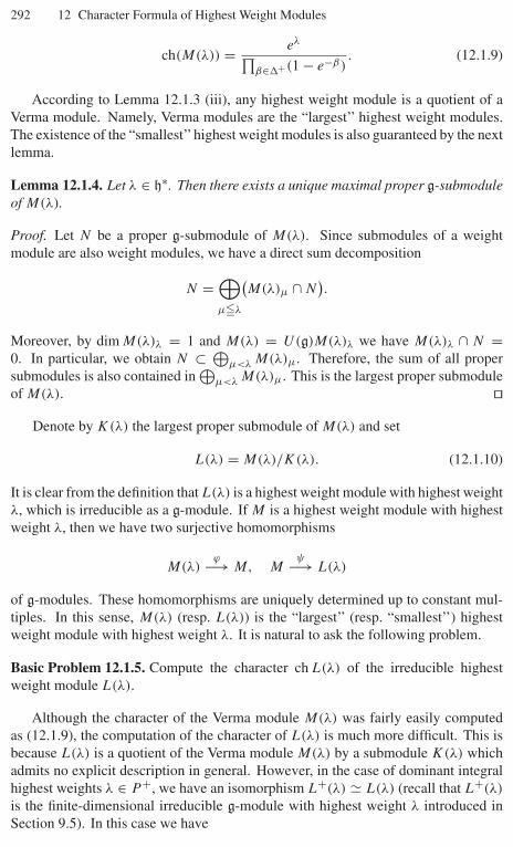
292 12 Character Formula of Highest Weight Modules
ch(M(λ)) = eλ∏β∈�+(1 − e−β)
. (12.1.9)
According to Lemma 12.1.3 (iii), any highest weight module is a quotient of aVerma module. Namely, Verma modules are the “largest’’ highest weight modules.The existence of the “smallest’’highest weight modules is also guaranteed by the nextlemma.
Lemma 12.1.4. Let λ ∈ h∗. Then there exists a unique maximal proper g-submoduleof M(λ).
Proof. Let N be a proper g-submodule of M(λ). Since submodules of a weightmodule are also weight modules, we have a direct sum decomposition
N =⊕µ�λ
(M(λ)µ ∩ N
).
Moreover, by dim M(λ)λ = 1 and M(λ) = U(g)M(λ)λ we have M(λ)λ ∩ N =0. In particular, we obtain N ⊂ ⊕
µ<λ M(λ)µ. Therefore, the sum of all propersubmodules is also contained in
⊕µ<λ M(λ)µ. This is the largest proper submodule
of M(λ). ��Denote by K(λ) the largest proper submodule of M(λ) and set
L(λ) = M(λ)/K(λ). (12.1.10)
It is clear from the definition that L(λ) is a highest weight module with highest weightλ, which is irreducible as a g-module. If M is a highest weight module with highestweight λ, then we have two surjective homomorphisms
M(λ)ϕ−→ M, M
ψ−→ L(λ)
of g-modules. These homomorphisms are uniquely determined up to constant mul-tiples. In this sense, M(λ) (resp. L(λ)) is the “largest’’ (resp. “smallest’’) highestweight module with highest weight λ. It is natural to ask the following problem.
Basic Problem 12.1.5. Compute the character ch L(λ) of the irreducible highestweight module L(λ).
Although the character of the Verma module M(λ) was fairly easily computedas (12.1.9), the computation of the character of L(λ) is much more difficult. This isbecause L(λ) is a quotient of the Verma module M(λ) by a submodule K(λ) whichadmits no explicit description in general. However, in the case of dominant integralhighest weights λ ∈ P +, we have an isomorphism L+(λ) � L(λ) (recall that L+(λ)
is the finite-dimensional irreducible g-module with highest weight λ introduced inSection 9.5). In this case we have

12.1 Highest weight modules 293
ch(L(λ)) =∑
w∈W (−1)l(w)ew(λ+ρ)−ρ∏β∈�+(1 − e−β)
(12.1.11)
=∑w∈W
(−1)l(w) ch(M(w(λ + ρ) − ρ))
by Weyl’s character formula. Therefore, our problem is to generalize the celebratedWeyl character formula to general highest weights.
Lemma 12.1.6. Let M be a highest weight module with highest weight λ. Then forany z ∈ z = (the center of U(g)) and m ∈ M we have
zm = χλ+ρ(z)m.
Proof. Let m0 be a highest weight vector of M . By M = U(g)m0 it is enough toshow that zm0 = χλ+ρ(z)m0 for any z ∈ z. Let us write
z = u + v (u ∈ U(h) ∼= C[h∗], v ∈ n−U(g) ∩ U(g)n)
(see Lemma 9.4.4). By nm0 = 0 we have zm0 = um0 = u(λ)m0. Moreover, by thedefinition of the Harish-Chandra homomorphism we obtain u(λ) = (γ (z))(λ+ρ) =χλ+ρ(z). ��Proposition 12.1.7. Let M be a highest weight g-module with highest weight λ. ThenM has a composition series of finite length, and each composition factor in it isisomorphic to an irreducible g-module L(µ) associated to µ ∈ h∗ satisfying thecondition
µ � λ, µ + ρ ∈ W(λ + ρ). (12.1.12)
Proof. If M is irreducible, then our assertion is obvious. So suppose that M is notirreducible and take a proper submodule N = 0 of M . Then N is a weight module,and any weight ν of N is a weight of M . Since N is a proper submodule, this weightν must satisfy ν < λ. We can choose a weight µ (µ < λ) of N which is maximal inthe set of weights of N because the number of µ’s satisfying ν � µ < λ is finite. If m
is a non-zero vector of Nµ, then by gαNµ ⊂ Nµ+α and the maximality of µ impliesnm = 0. This implies that U(g)m is a highest weight module with highest weight µ.Hence we may assume from the beginning that N is a highest weight module withhighest weight µ. In this situation, we can prove
µ < λ, µ + ρ ∈ W(λ + ρ). (12.1.13)
Indeed, by Lemma 12.1.6 for any z ∈ z we have z|M = χλ+ρ(z)id and z|N =χµ+ρ(z)id. Consequently we get χλ+ρ = χµ+ρ . Hence it follows from Propo-sition 9.4.5 that µ + ρ ∈ W(λ + ρ). If N is not irreducible, applying the sameargument to N itself we can find a proper highest weight submodule N ′ = 0 of N
whose highest weight µ′ satisfies
µ′ < µ < λ, µ′ + ρ ∈ W(µ + ρ) = W(λ + ρ).
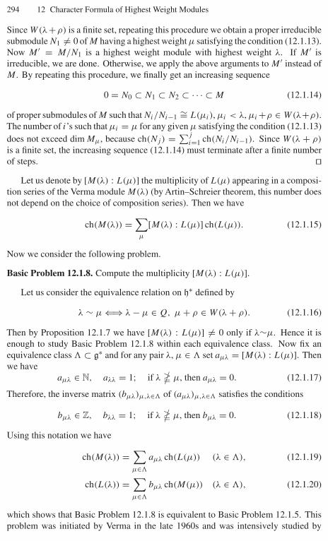
294 12 Character Formula of Highest Weight Modules
Since W(λ+ρ) is a finite set, repeating this procedure we obtain a proper irreduciblesubmodule N1 = 0 of M having a highest weight µ satisfying the condition (12.1.13).Now M ′ = M/N1 is a highest weight module with highest weight λ. If M ′ isirreducible, we are done. Otherwise, we apply the above arguments to M ′ instead ofM . By repeating this procedure, we finally get an increasing sequence
0 = N0 ⊂ N1 ⊂ N2 ⊂ · · · ⊂ M (12.1.14)
of proper submodules of M such that Ni/Ni−1 ∼= L(µi), µi < λ, µi +ρ ∈ W(λ+ρ).The number of i’s such that µi = µ for any given µ satisfying the condition (12.1.13)does not exceed dim Mµ, because ch(Nj ) = ∑j
i=1 ch(Ni/Ni−1). Since W(λ + ρ)
is a finite set, the increasing sequence (12.1.14) must terminate after a finite numberof steps. ��
Let us denote by [M(λ) : L(µ)] the multiplicity of L(µ) appearing in a composi-tion series of the Verma module M(λ) (by Artin–Schreier theorem, this number doesnot depend on the choice of composition series). Then we have
ch(M(λ)) =∑µ
[M(λ) : L(µ)] ch(L(µ)). (12.1.15)
Now we consider the following problem.
Basic Problem 12.1.8. Compute the multiplicity [M(λ) : L(µ)].Let us consider the equivalence relation on h∗ defined by
λ ∼ µ ⇐⇒ λ − µ ∈ Q, µ + ρ ∈ W(λ + ρ). (12.1.16)
Then by Proposition 12.1.7 we have [M(λ) : L(µ)] = 0 only if λ∼µ. Hence it isenough to study Basic Problem 12.1.8 within each equivalence class. Now fix anequivalence class � ⊂ g∗ and for any pair λ, µ ∈ � set aµλ = [M(λ) : L(µ)]. Thenwe have
aµλ ∈ N, aλλ = 1; if λ � µ, then aµλ = 0. (12.1.17)
Therefore, the inverse matrix (bµλ)µ,λ∈� of (aµλ)µ,λ∈� satisfies the conditions
bµλ ∈ Z, bλλ = 1; if λ � µ, then bµλ = 0. (12.1.18)
Using this notation we have
ch(M(λ)) =∑µ∈�
aµλ ch(L(µ)) (λ ∈ �), (12.1.19)
ch(L(λ)) =∑µ∈�
bµλ ch(M(µ)) (λ ∈ �), (12.1.20)
which shows that Basic Problem 12.1.8 is equivalent to Basic Problem 12.1.5. Thisproblem was initiated by Verma in the late 1960s and was intensively studied by
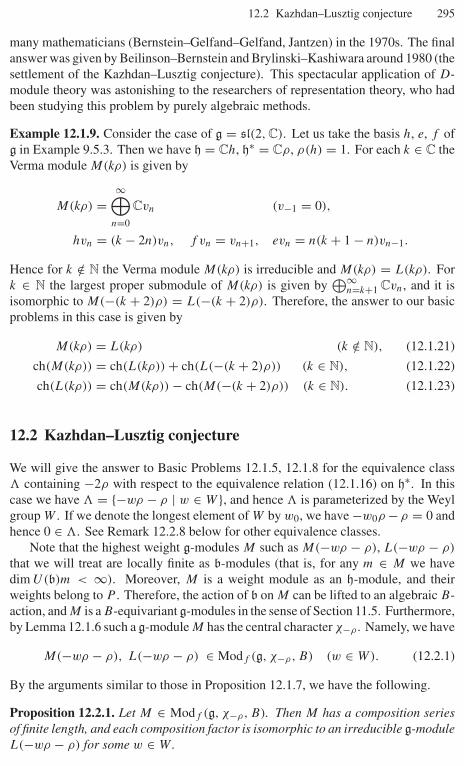
12.2 Kazhdan–Lusztig conjecture 295
many mathematicians (Bernstein–Gelfand–Gelfand, Jantzen) in the 1970s. The finalanswer was given by Beilinson–Bernstein and Brylinski–Kashiwara around 1980 (thesettlement of the Kazhdan–Lusztig conjecture). This spectacular application of D-module theory was astonishing to the researchers of representation theory, who hadbeen studying this problem by purely algebraic methods.
Example 12.1.9. Consider the case of g = sl(2, C). Let us take the basis h, e, f ofg in Example 9.5.3. Then we have h = Ch, h∗ = Cρ, ρ(h) = 1. For each k ∈ C theVerma module M(kρ) is given by
M(kρ) =∞⊕
n=0
Cvn (v−1 = 0),
hvn = (k − 2n)vn, f vn = vn+1, evn = n(k + 1 − n)vn−1.
Hence for k /∈ N the Verma module M(kρ) is irreducible and M(kρ) = L(kρ). Fork ∈ N the largest proper submodule of M(kρ) is given by
⊕∞n=k+1 Cvn, and it is
isomorphic to M(−(k + 2)ρ) = L(−(k + 2)ρ). Therefore, the answer to our basicproblems in this case is given by
M(kρ) = L(kρ) (k /∈ N), (12.1.21)
ch(M(kρ)) = ch(L(kρ)) + ch(L(−(k + 2)ρ)) (k ∈ N), (12.1.22)
ch(L(kρ)) = ch(M(kρ)) − ch(M(−(k + 2)ρ)) (k ∈ N). (12.1.23)
12.2 Kazhdan–Lusztig conjecture
We will give the answer to Basic Problems 12.1.5, 12.1.8 for the equivalence class� containing −2ρ with respect to the equivalence relation (12.1.16) on h∗. In thiscase we have � = {−wρ − ρ | w ∈ W }, and hence � is parameterized by the Weylgroup W . If we denote the longest element of W by w0, we have −w0ρ − ρ = 0 andhence 0 ∈ �. See Remark 12.2.8 below for other equivalence classes.
Note that the highest weight g-modules M such as M(−wρ − ρ), L(−wρ − ρ)
that we will treat are locally finite as b-modules (that is, for any m ∈ M we havedim U(b)m < ∞). Moreover, M is a weight module as an h-module, and theirweights belong to P . Therefore, the action of b on M can be lifted to an algebraic B-action, and M is a B-equivariant g-modules in the sense of Section 11.5. Furthermore,by Lemma 12.1.6 such a g-module M has the central character χ−ρ . Namely, we have
M(−wρ − ρ), L(−wρ − ρ) ∈ Modf (g, χ−ρ, B) (w ∈ W). (12.2.1)
By the arguments similar to those in Proposition 12.1.7, we have the following.
Proposition 12.2.1. Let M ∈ Modf (g, χ−ρ, B). Then M has a composition seriesof finite length, and each composition factor is isomorphic to an irreducible g-moduleL(−wρ − ρ) for some w ∈ W .
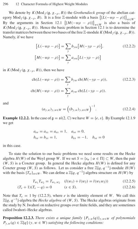
296 12 Character Formula of Highest Weight Modules
We denote by K(Modf (g, χ−ρ, B)) the Grothendieck group of the abelian cat-egory Modf (g, χ−ρ, B). It is a free Z-module with a basis
{[L(−wρ − ρ)]}w∈W
.By the arguments in Section 12.1
{[M(−wρ − ρ)]}w∈W
is also a basis ofK(Modf (g, χ−ρ, B)). Hence the basic problem in Section 12.1 is to determine thetransfer matrices between these two bases of the free Z-module K(Modf (g, χ−ρ, B)).Namely, if we have [
L(−wρ − ρ)] =
∑y
byw
[M(−yρ − ρ)
], (12.2.2)
[M(−wρ − ρ)
] =∑
y
ayw
[L(−yρ − ρ)
]in K(Modf (g, χ−ρ, B)), then we have
ch(L(−wρ − ρ)) =∑
y
byw ch(M(−yρ − ρ)), (12.2.3)
ch(M(−wρ − ρ)) =∑
y
ayw ch(L(−yρ − ρ)).
and
(ay,w)y,w∈W =((by,w)y,w∈W
)−1. (12.2.4)
Example 12.2.2. In the case of g = sl(2, C) we have W = {e, s}. By Example 12.1.9we get
aee = ass = aes = 1, ase = 0,
bee = bss = 1, bes = −1, bse = 0
in this case.
To state the solution to our basic problems we need some results on the Heckealgebra H(W) of the Weyl group W . If we set S = {sα | α ∈ $} ⊂ W , then the pair(W, S) is a Coxeter group. In general the Hecke algebra H(W) is defined for anyCoxeter group (W, S) as follows. Let us consider a free Z[q, q−1]-module H(W)
with the basis {Tw}w∈W . We can define a Z[q, q−1]-algebra structure on H(W) by
Tw1Tw2 = Tw1,w2 (l(w1) + l(w2) = l(w1w2)) (12.2.5)
(Ts + 1)(Ts − q) = 0 (s ∈ S). (12.2.6)
Note that Te = 1 by (12.2.5), where e is the identity element of W . We call thisZ[q, q−1]-algebra the Hecke algebra of (W, S). The Hecke algebras originate fromthe study by N. Iwahori on reductive groups over finite fields, and they are sometimescalled Iwahori–Hecke algebras.
Proposition 12.2.3. There exists a unique family {Py,w(q)}y,w∈W of polynomialsPy,w(q) ∈ Z[q] (y, w ∈ W ) satisfying the following conditions:
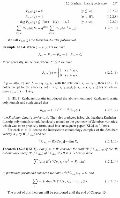
12.2 Kazhdan–Lusztig conjecture 297
Py,w(q) = 0 (y � w), (12.2.7)
Pw,w(q) = 1 (w ∈ W), (12.2.8)
deg Py,w(q) � (l(w) − l(y) − 1)/2 (y < w), (12.2.9)∑y�w
Py,w(q)Ty = ql(w)∑y�w
Py,w(q−1)T −1y−1. (12.2.10)
We call Py,w(q) the Kazhdan–Lusztig polynomial.
Example 12.2.4. When g = sl(2, C) we have
Pee = Pss = Pes = 1, Pse = 0.
More generally, in the case where |S| � 2 we have
Py,w(q) ={
1 (y � w),
0 (y � w).(12.2.11)
If g = sl(4, C) and S = {s1, s2, s3} with the relation s1s3 = s3s1, then (12.2.11)holds except for the cases (y, w) = (s2, s2s1s3s2), (s1s3, s1s3s2s3s1) for which wehave Py,w(q) = 1 + q.
In [KL1] Kazhdan–Lusztig introduced the above-mentioned Kazhdan–Lusztigpolynomials and conjectured that
by,w = (−1)l(w)−l(y)Py,w(1) (12.2.12)
(the Kazhdan–Lusztig conjecture). They also predicted in loc. cit. that these Kazhdan–Lusztig polynomials should be closely related to the geometry of Schubert varieties,which was more precisely formulated in a subsequent paper [KL2] as follows.
For each w ∈ W denote the intersection cohomology complex of the Schubertvariety Xw by IC(CXw) and set
πCXw = IC(CXw)[− dim Xw]. (12.2.13)
Theorem 12.2.5 ([KL2]). For y, w ∈ W consider the stalk Hi(πCXw)yB of the ithcohomology sheaf Hi(πCXw) of πCXw at yB ∈ X. Then we have∑
i
(dim Hi(πCXw)yB)qi2 = Py,w(q). (12.2.14)
In particular, for an odd number i we have Hi(πCXw)yB = 0, and∑j
(−1)j dim Hj (πCXw)yB = Py,w(1). (12.2.15)
The proof of this theorem will be postponed until the end of Chapter 13.
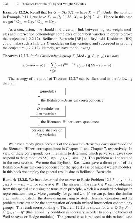
298 12 Character Formula of Highest Weight Modules
Example 12.2.6. Recall that for G = SL2(C) we have X = P1. Under the notationin Example 9.11.1, we have Xs = U1 ∼= A1, Xe = {eB} ∼= A0. Hence in this casewe get πCXs = CX, πCXe = CXe .
As a conclusion, one should find a certain link between highest weight mod-ules and intersection cohomology complexes of Schubert varieties in order to provethe conjecture (12.2.12). Beilinson–Bernstein [BB] and Brylinski–Kashiwara [BK]could make such a link via D-modules on flag varieties, and succeeded in provingthe conjecture (12.2.12). Namely, we have the following.
Theorem 12.2.7. In the Grothendieck group K(Modf (g, B, χ−ρ)) we have
[L(−wρ − ρ)] =∑y�w
(−1)l(w)−l(y)Py,w(1)[M(−yρ − ρ)].
The strategy of the proof of Theorem 12.2.7 can be illustrated in the followingdiagram:
g-modules�⏐⏐ the Beilinson–Bernstein correspondence
D-modules onflag varieties�⏐⏐ the Riemann–Hilbert correspondence
perverse sheaves onflag varieties
We have already given accounts of the Beilinson–Bernstein correspondence andthe Riemann–Hilbert correspondence in Chapter 11 and Chapter 7, respectively. Inview of these correspondences it remains to determine which perverse sheaves cor-respond to the g-modules M(−wρ − ρ), L(−wρ − ρ). This problem will be studiedin the next section. We note that Brylinski–Kashiwara gave a direct proof of theBeilinson–Bernstein correspondence for the special case of highest weight modules.In this book we employ the general results due to Beilinson–Bernstein.
Remark 12.2.8. We have described the answer to Basic Problem 12.1.5 only in thecase λ = −wρ − ρ for some w ∈ W . The answer in the case λ ∈ P can be obtainedfrom this special case using the translation principle, which is a standard technique inrepresentation theory. More generally, for general λ ∈ h∗ we can perform the similararguments indicated in the above diagram using twisted differential operators, and theproblem turns out to be the computation of certain twisted intersection cohomologygroups. The result corresponding to Theorem 12.2.5 is shown for λ ∈ Q ⊗Z P ⊂C ⊗Z P = h∗ (this rationality condition is necessary in order to apply the theory ofWeil sheaves or Hodge modules). The general case is reduced to this rational case
12.3 D-modules associated to highest weight modules 299
by using Jantzen’s deformation argument [J]. The final answer is given in terms ofKazhdan–Lusztig polynomials of the subgroup
W(λ) = {w ∈ W | wλ − λ ∈ Q}of W . For details we refer to [KT7]. We finally note that Kashiwara’s conjectureon semisimple holonomic system (see Kashiwara [Kas17]), which would in partic-ular give the result corresponding to Theorem 12.2.5 for all λ, seems to have beenestablished by a recent remarkable progress (see Drinfeld [Dr], Gaitsgory [Gai], andMochizuki [Mo] and Sabbah [Sab2]).
12.3 D-modules associated to highest weight modules
In Chapter 11 we proved the equivalence of categories
Modf (g, B, χ−ρ)∼−→ Modc(DX, B) = Modrh(DX, B). (12.3.1)
Let us denote by Mw, Lw the objects in Modrh(DX, B) which correspond toM(−wρ − ρ), L(−wρ − ρ) ∈ Modf (g, B, χ−ρ), respectively. Namely, we set
Mw = DX ⊗U(g) Mw, Lw = DX ⊗U(g) Lw (w ∈ W). (12.3.2)
In view of (12.3.1) our problem of determining the transfer matrix between twobases {[M(−wρ − ρ)]}w∈W , {[L(−wρ − ρ)]}w∈W of the Grothendieck groupK(Modf (g, B, χ−ρ)) can be reduced to determining the transfer matrix betweentwo bases {[Mw]}w∈W , {[Lw]}w∈W of K(Modrh(DX, B)). For this purpose, weneed more concrete descriptions of Mw and Lw.
For w ∈ W let iw : Xw ↪→ X be the embedding. Then Xw\Xw is a divisor ofXw by Theorem 9.9.5, and hence iw is an affine morphism. Let us set
Nw =∫
iw
OXw = iw∗(DX←Xw ⊗DXwOXw) (w ∈ W). (12.3.3)
Then we have Nw ∈ Modrh(DX, B) because Xw is a B-orbit.
Lemma 12.3.1. Let w ∈ W . Then
(i) We have ch(�(X, Nw)) = ch(M(−wρ − ρ)). In particular, in the Grothendieckgroup K(Modrh(DX, B)) we obtain [Mw] = [Nw].
(ii) The only DX-submodule of Nw whose support is contained in Xw\Xw is zero.
Proof. (i) We define two subalgebras of g by
n1 =⊕
α∈�+∩w(�+)
g−α, n2 =⊕
α∈�+∩(−w(�+))
gα.
300 12 Character Formula of Highest Weight Modules
Then the corresponding unipotent subgroups N1, N2 of G with the propertiesLie(N1) = n1, Lie(N2) = n2 are determined. For each w ∈ W = NG(H)/H we fixa representative w ∈ NG(H) of it and define a morphism ϕ : N1 × N2 → X by
ϕ(n1, n2) = n1n2wB (n1 ∈ N1, n2 ∈ N2).
Then ϕ is an open embedding satisfying ϕ({e} × N2) = Xw. Namely, setting V =Im(ϕ) we obtain the following commutative diagram:
N2
�|{e} × N2 iw
�
N1 × N2
∼
ϕ∼↪−→
Xw
�
V X
�
�
��
��
���
Therefore, we have
�(X, Nw) = �(X , iw∗
(DX←Xw ⊗DXw
OXw
))= �
(Xw , DX←Xw ⊗DXw
OXw
)= �
(Xw , DV ←Xw ⊗DXw
OXw
)∼= �
(N2 , DN1×N2←N2 ⊗DN2
ON2
).
Moreover, by
DN1×N2←N2 =(DN1,e ⊗ON1,e
C)
⊗C
(�⊗−1
N1,e ⊗ON1,eC)
⊗C DN2 ,
we obtain
�(X, Nw) ∼=(DN1,e ⊗ON1,e
C)
⊗C
(�⊗−1
N1,e ⊗ON1,eC)
⊗C �(N2, ON2).
Identifying n1 with the set of right-invariant vector fields on N1, we get DN1∼=
U(n1)⊗CON1 and hence DN1,e ⊗ON1,eC ∼= U(n1). Furthermore, we have obviously
�⊗−1N1,e ⊗ON1 ,e C ∼= ∧p n1 (p = dim n1). Since N2 is a unipotent algebraic group,
the exponential map exp : n2 → N2 is an isomorphism of algebraic varieties, andhence we obtain �(N2, ON2)
∼= �(n2, On2) = S(n∗2). Therefore, we have
�(X, Nw) ∼= U(n1) ⊗C
p∧n1 ⊗C S(n∗
2). (12.3.4)
Recall that our problem was to study the action of h on �(X, Nw). Let us define anH -action on N1 × N2 by

12.3 D-modules associated to highest weight modules 301
t · (n1, n2) = (tn1t−1, tn2t−1) (t ∈ H, n1 ∈ N1, n2 ∈ N2).
Then ϕ is H -equivariant, from which we see that (12.3.4) is an isomorphism of h-modules. Therefore, we obtain ch(�(X, Nw)) = ch(U(n1)) ch(
∧pn1) ch(S(n∗2)).
We easily see that
ch(U(n1)) = 1∏α∈�+∩w(�+)(1 − e−α)
, (12.3.5)
ch(S(n∗2)) = 1∏
α∈�+∩(−w(�+))(1 − e−α). (12.3.6)
Moreover, by ρ = 12
∑α∈�+ α we have
∑α∈�−∩w(�−) α = −wρ − ρ, and hence
ch(∧p
n1) = e−wρ−ρ. (12.3.7)
Therefore, we finally get
ch(�(X, Nw)) = e−wρ−ρ∏α∈�+(1 − e−α)
= ch(M(−wρ − ρ)).
(ii) Set Z = X\V and let j : V ↪→ X be the open embedding. Then we have adistinguished triangle
R�Z(Nw) −→ Nw −→ j∗(Nw|V )+1−→ .
It follows from the definition of Nw that Nw → j∗(Nw|V ) is an isomorphism, andhence we get R�Z(Nw) = 0. In particular, we have �Z(Nw) = 0. Thus the onlyDX-submodule of Nw whose support is contained in Z is zero. By Xw\Xw ⊂ Z theassertion (ii) is now clear. ��
We denote by L(Xw, OXw) the minimal extension (see Section 3.4) of the regularholonomic DXw -module OXw . We have obviously L(Xw, OXw) ∈ Modrh(DX, B).
Proposition 12.3.2. Let w ∈ W . Then we have
(i) Lw = L(Xw, OXw),
(ii) Mw = DNw (here D = DX is the dualizing functor introduced in Section 2.6).
Proof. (i) By the results in Section 11.6 and the fact that Xanw is simply connected,
the set P of isomorphism classes of irreducible objects in Modrh(DX, B) is givenby P = {L(Xw, OXw)}w∈W . On the other hand, the set of isomorphism classes ofirreducible objects in Modf (g, B, χ−ρ) is {L(−wρ − ρ)}w∈W . So by the definitionof Lw we get P = {Lw}w∈W . This means that for any w ∈ W there exists a uniquey ∈ W such that Lw = L(Xy, OXy ). By the definition of Mw and Lw we seethat Lw = L(Xy, OXy ) is a composition factor of Mw (note that L(−wρ − ρ)
is a composition factor of M(−wρ − ρ)). Recall that by Lemma 12.3.1 (i) thecomposition factors of Mw and those of Nw are the same. Hence Lw = L(Xy, OXy )
302 12 Character Formula of Highest Weight Modules
is a composition factor of Nw. By the results in Section 3.4, any composition factorof Nw should be written as L(Xx, OXx ) for some x � w, which shows that y � w.Hence we obtain y = w by an induction on w with respect to the Bruhat order.
(ii) Since the irreducible objects L(Xw, OXw) of Modrh(DX, B) are self-dual,the composition factors of M ∈ Modrh(DX, B) and those of DM coincide. Hencewe have ch(�(X, M)) = ch(�(X, DM)). In particular, we get ch(�(X, DNw)) =ch(�(X, Nw)) = ch(M(−wρ −ρ)). We see from this that U(g) ·�(X, DNw)−wρ−ρ
is a highest weight module with highest weight −wρ − ρ. Hence there exists anon-trivial homomorphism f1 : M(−wρ − ρ) → �(X, DNw) of g-modules. ThenL(−wρ−ρ) is not a composition factor of N = Coker(f1). From the exact sequence
M(−wρ − ρ)f1−→ �(X, DNw) −→ N −→ 0 (12.3.8)
of g-module, we obtain an exact sequence
Mwf2−→ DNw −→ N −→ 0 (12.3.9)
of DX-modules, where N = DX ⊗U(g) N . Taking its dual we obtain also the exactsequence
0 −→ DN −→ Nwf3−→ DMw. (12.3.10)
Since Lw is not contained in the set of composition factors of N and DN , the supportof DN is contained in Xw\Xw. Hence we get DN = 0 by Lemma 12.3.1 (ii).It follows that N = 0 and hence N = 0. In other words f1 is surjective. Weconclude from this that f1 is an isomorphism by ch(�(X, DNw)) = ch(M(−wρ −ρ)). Therefore, f2 is also an isomorphism. ��
By the Riemann–Hilbert correspondence we get the following.
Corollary 12.3.3.(i) DRX(Mw) = CXw [dim Xw] (w ∈ W).
(ii) DRX(Lw) = πCXw [dim Xw] (w ∈ W).
Proof of Theorem 12.2.7. By the definition of Mw and Lw it is enough to show that
[Lw] =∑y�w
(−1)l(w)−l(y)Py,w(1)[My] (w ∈ W) (12.3.11)
in the Grothendieck group K(Modrh(DX, B)). Let us define a homomorphism ϕ :K(Modrh(DX, B)) → Z[W ] of Z-modules by
ϕ([M]) =∑y∈w
(∑i
(−1)i dim Hi(DRX(M))yB
)y. (12.3.12)
Note that ϕ is well defined since we are taking an alternating sum of the dimensionsof cohomology groups. Then by Corollary 12.3.3 (i) we have ϕ([Mw]) = (−1)l(w)w
12.3 D-modules associated to highest weight modules 303
and ϕ is an isomorphism of Z-modules. Furthermore, by Corollary 12.3.3 (ii) andTheorem 12.2.5 we obtain
ϕ([Lw]) = (−1)l(w)∑
y
(∑i
(−1)i dim Hi(πCXw)yB
)y
= (−1)l(w)∑y�w
Py,w(1)y
=∑y�w
(−1)l(w)−l(y)Py,w(1)ϕ([My]),
from which our claim (12.3.11) is clear. ��
13
Hecke Algebras and Hodge Modules
In this chapter we give geometric realization of group algebras of Weyl groups (resp.Hecke algebras) via D-modules (resp. via Hodge modules). We also include a proofof Kazhdan–Lusztig’s theorem (Theorem 12.2.5, i.e., the calculation of intersectioncohomology complexes of Schubert varieties) using the theory of Hodge modules.
13.1 Weyl groups and D-modules
Let �G = {(g, g) | g ∈ G} � G be the diagonal subgroup of G × G and considerthe diagonal action of �G on X × X. Let us give the orbit decomposition of X × X
for this �G-action. Since G acts transitively on X, we can take as a representative ofeach �G-orbit in X×X an element of the form (eB, gB). Furthermore, two elements(eB, g1B) and (eB, g2B) lie in the same �G-orbit if and only if g1B and g2B lie inthe same B-orbit. Namely, there exists a bijection between the set of �G-orbits inX × X and that of B-orbits in X. Under this bijection, the B-orbit Xw (w ∈ W ) inX corresponds to the �G-orbit
Zw = �G(eB, wB) (w ∈ W) (13.1.1)
in X × X. Hence we obtain the orbit decomposition
X × X =∐
w∈W
Zw. (13.1.2)
We can also describe geometric properties of �G-orbits in X × X from the ones ofB-orbits in X as follows. Define morphisms pk : X × X → X, ik : X → X × X
(k = 1, 2) by
p1(a, b) = a, p2(a, b) = b, i1(a) = (eB, a), i2(a) = (a, eB). (13.1.3)
Then we can regard X × X via the projection p1 as a G-equivariant fiber bundle onX = G/B whose fiber i1(X) over eB ∈ X is isomorphic to X. Moreover, for each
306 13 Hecke Algebras and Hodge Modules
w ∈ W , Zw is a G-equivariant subbundle of X × X whose fiber over eB ∈ X isisomorphic to i−1
1 (Zw) = Xw. Hence we have
X × X = GB× X, Zw = G
B× Xw (w ∈ W) (13.1.4)
under the standard notation of associated fiber bundles (we can also obtain similardescriptions using p2 and i2 in which Zw−1 corresponds to Xw).
Namely, the �G-orbit decomposition of X×X corresponds to that of the B-orbitdecomposition of X including geometric natures such as singularities of the closures.In particular, we have the following by Theorem 9.9.5.
Proposition 13.1.1.(i) Zw = ∐
y�w Zy .(ii) dim Zw = dim X + l(w).
In this chapter we will deal with �G-equivariant D-modules on X × X insteadof B-equivariant D-modules on X considered in Chapter 12. Indeed, we have thefollowing correspondence between them.
Proposition 13.1.2. The inverse image functors Li∗1 = i†1 [dim X] and Li∗2 =
i†2 [dim X] of D-modules induce the following equivalences of categories:
i∗1 : Modc(DX×X, �G)∼−→ Modc(DX, B),
i∗2 : Modc(DX×X, �G)∼−→ Modc(DX, B).
We omit the proof because it follows easily from the above geometric observa-tions.
Note thatHpLi∗k (M) = 0 (p = 0, k = 1, 2)
holds for any M ∈ Modc(DX×X, �G). Note also that
Modc(DX×X, �G) = Modrh(DX×X, �G) (13.1.5)
by Theorem 11.6.1. For w ∈ W consider the embedding jw : Zw ↪→ X × X and set
Nw =∫
jw
OZw, Mw = DNw, Lw = L(Zw, OZw). (13.1.6)
They are objects in Modc(DX×X, �G). Moreover, we have
i∗1 (Nw) = Nw,
i∗2 (Nw) = Nw−1 ,
i∗1 (Mw) = Mw,
i∗2 (Mw) = Mw−1 ,
i∗1 (Lw) = Lw,
i∗2 (Lw) = Lw−1
(13.1.7)
under the notation of Chapter 12. Therefore, we get the following proposition.
13.1 Weyl groups and D-modules 307
Proposition 13.1.3.(i) K(Modc(DX×X, �G)) = ⊕
w∈W Z[Mw] = ⊕w∈W Z[Lw].
(ii) For any w ∈ W we have [Mw] = [Nw].Let us define morphisms p13 : X × X × X → X × X and r : X × X × X →
X × X × X × X by
p13(a, b, c) = (a, c) r(a, b, c) = (a, b, b, c). (13.1.8)
Remark 13.1.4. For any M, N ∈ Modc(DX×X, �G) and p = 0 , we can prove thatHpLr∗(M � N ) = 0 (see the proof of Proposition 13.2.7 (i) below).
Proposition 13.1.5.(i) The Grothendieck group K(Modc(DX×X, �G)) has a ring structure defined by
[M] · [N ] =∑
k
(−1)k
[Hk
∫p13
r∗(M � N )
].
(ii) The ring K(Modc(DX×X, �G)) is isomorphic to the group ring Z[W ] of theWeyl group W by the correspondence [Mw] ↔ (−1)l(w)w.
Proof. (i)The proof is a simple application of the base change theorem for D-modules.By
([M] · [N ]) · [L] =∑
k
(−1)k
[Hk
∫p13
r∗((∫
p13
r∗(M � N )
)� L
)],
[M] · ([N ] · [L]) =∑
k
(−1)k
[Hk
∫p13
r∗(
M �(∫
p13
r∗(N � L)
))],
it suffices to prove that∫p13
r∗((∫
p13
r∗(M � N )
)� L
)=∫
p13
r∗(
M �(∫
p13
r∗(N � L)
)).
The left-hand side (LHS) of the above formula is given by
(LHS) =∫
p13
r∗∫
p13×1×1(r × 1 × 1)∗(M � N � L).
Since the diagram
X4 1×r−−−−→ X5
p13×1
⏐⏐ ⏐⏐p13×1×1
X3 r−−−−→ X4
is a cartesian square (i.e., X4 is the fiber product of r and p13 × 1 × 1), we get
308 13 Hecke Algebras and Hodge Modules
(LHS) =∫
p13
∫p13×1
(1 × r)∗(r × 1 × 1)∗(M � N � L)
=∫
p13◦(p13×1)
((r × 1 × 1) ◦ (1 × r)
)∗(M � N � L).
Similarly the right-hand side (RHS) can be rewritten as follows:
(RHS) =∫
p13◦(1×p13)
((1 × 1 × r) ◦ (r × 1)
)∗(M � N � L).
Therefore, the assertion (i) follows from p13 ◦ (p13 × 1) = p13 ◦ (1 × p13) and(r × 1 × 1) ◦ (1 × r) = (1 × 1 × r) ◦ (r × 1).
(ii) It is enough to prove the following two formulas:
[My] · [Mw] = [Myw] (l(y) + l(w) = l(yw)), (13.1.9)
[Ms]2 = [Me] (s ∈ S), (13.1.10)
where S = {sα | α ∈ $}. We first show (13.1.9). By [Mw] = [Nw] = [∫jw
OZw ]we get
[My] · [Mw] =∑
k
(−1)k
[Hk
∫p13
r∗(∫
jy
OZy �∫
jw
OZw
)]
=∑
k
(−1)k
[Hk
∫p13
r∗∫
jy×jw
OZy×Zw
].
We see from l(y) + l(w) = l(yw) that for any (a, b) ∈ Zyw there exists a uniquec ∈ X such that (a, c) ∈ Zy and (c, b) ∈ Zw. Conversely, if (a, c) ∈ Zy and(c, b) ∈ Zw, then (a, b) ∈ Zyw. Hence if we define morphisms ϕ : Zyw → Zy ×Zw,ψ : Zyw → X3 by ϕ(a, b) = (a, c, c, b), ψ(a, b) = (a, c, b), then the diagram
Zywϕ−−−−→ Zy × Zw
ψ
⏐⏐ ⏐⏐jy×jw
X3 r−−−−→ X4
is the fiber product of r and jy ×jw. Therefore, it follows from this and p13◦ψ = jyw
that ∫p13
r∗∫
jy×jw
OZy×Zw =∫
p13
∫ψ
ϕ∗OZy×Zw =∫
jyw
OZyw = Nyw.
Hence we obtain (13.1.9). We next show (13.1.10). Note that Zs is smooth andZs = Zs � Ze. Moreover, Ze is a smooth closed subvariety of Zs of codimensionone. Let j ′
s : Zs → Zs , j ′e : Ze → Zs , js : Zs → X × X be the embeddings. Then
we have an exact sequence
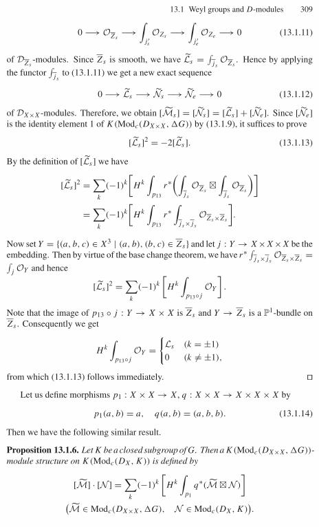
13.1 Weyl groups and D-modules 309
0 −→ OZs−→
∫j ′s
OZs −→∫
j ′e
OZe −→ 0 (13.1.11)
of DZs-modules. Since Zs is smooth, we have Ls = ∫
jsOZs
. Hence by applying
the functor∫
jsto (13.1.11) we get a new exact sequence
0 −→ Ls −→ Ns −→ Ne −→ 0 (13.1.12)
of DX×X-modules. Therefore, we obtain [Ms] = [Ns] = [Ls] + [Ne]. Since [Ne]is the identity element 1 of K(Modc(DX×X, �G)) by (13.1.9), it suffices to prove
[Ls]2 = −2[Ls]. (13.1.13)
By the definition of [Ls] we have
[Ls]2 =∑
k
(−1)k
[Hk
∫p13
r∗(∫
js
OZs�∫
js
OZs
)]=∑
k
(−1)k
[Hk
∫p13
r∗∫
js×js
OZs×Zs
].
Now set Y = {(a, b, c) ∈ X3 | (a, b), (b, c) ∈ Zs} and let j : Y → X×X×X be theembedding. Then by virtue of the base change theorem, we have r∗ ∫
js×jsOZs×Zs
=∫jOY and hence
[Ls]2 =∑
k
(−1)k
[Hk
∫p13◦j
OY
].
Note that the image of p13 ◦ j : Y → X × X is Zs and Y → Zs is a P1-bundle onZs . Consequently we get
Hk
∫p13◦j
OY ={
Ls (k = ±1)
0 (k = ±1),
from which (13.1.13) follows immediately. ��Let us define morphisms p1 : X × X → X, q : X × X → X × X × X by
p1(a, b) = a, q(a, b) = (a, b, b). (13.1.14)
Then we have the following similar result.
Proposition 13.1.6. Let K be a closed subgroup of G. Then a K(Modc(DX×X, �G))-module structure on K(Modc(DX, K)) is defined by
[M] · [N ] =∑
k
(−1)k
[Hk
∫p1
q∗(M � N )
](M ∈ Modc(DX×X, �G), N ∈ Modc(DX, K)
).
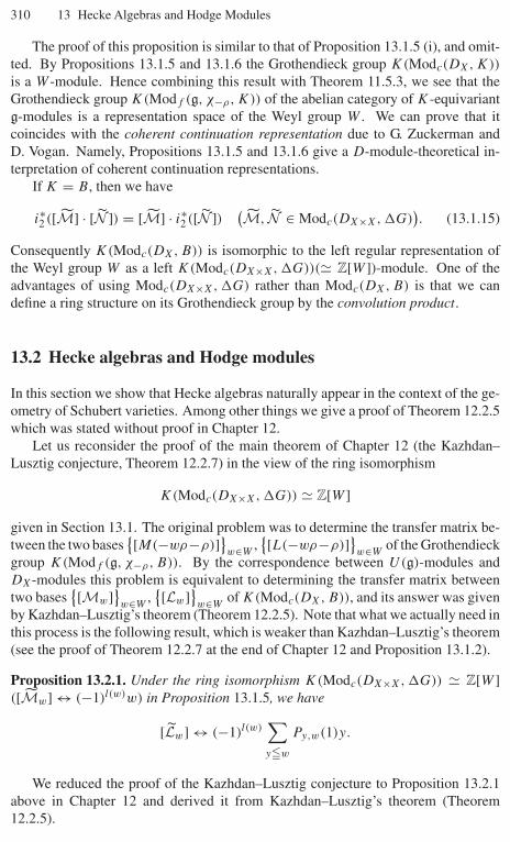
310 13 Hecke Algebras and Hodge Modules
The proof of this proposition is similar to that of Proposition 13.1.5 (i), and omit-ted. By Propositions 13.1.5 and 13.1.6 the Grothendieck group K(Modc(DX, K))
is a W -module. Hence combining this result with Theorem 11.5.3, we see that theGrothendieck group K(Modf (g, χ−ρ, K)) of the abelian category of K-equivariantg-modules is a representation space of the Weyl group W . We can prove that itcoincides with the coherent continuation representation due to G. Zuckerman andD. Vogan. Namely, Propositions 13.1.5 and 13.1.6 give a D-module-theoretical in-terpretation of coherent continuation representations.
If K = B, then we have
i∗2 ([M] · [N ]) = [M] · i∗2 ([N ]) (M, N ∈ Modc(DX×X, �G)
). (13.1.15)
Consequently K(Modc(DX, B)) is isomorphic to the left regular representation ofthe Weyl group W as a left K(Modc(DX×X, �G))(� Z[W ])-module. One of theadvantages of using Modc(DX×X, �G) rather than Modc(DX, B) is that we candefine a ring structure on its Grothendieck group by the convolution product.
13.2 Hecke algebras and Hodge modules
In this section we show that Hecke algebras naturally appear in the context of the ge-ometry of Schubert varieties. Among other things we give a proof of Theorem 12.2.5which was stated without proof in Chapter 12.
Let us reconsider the proof of the main theorem of Chapter 12 (the Kazhdan–Lusztig conjecture, Theorem 12.2.7) in the view of the ring isomorphism
K(Modc(DX×X, �G)) � Z[W ]given in Section 13.1. The original problem was to determine the transfer matrix be-tween the two bases
{[M(−wρ−ρ)]}w∈W
,{[L(−wρ−ρ)]}
w∈Wof the Grothendieck
group K(Modf (g, χ−ρ, B)). By the correspondence between U(g)-modules andDX-modules this problem is equivalent to determining the transfer matrix betweentwo bases
{[Mw]}w∈W
,{[Lw]}
w∈Wof K(Modc(DX, B)), and its answer was given
by Kazhdan–Lusztig’s theorem (Theorem 12.2.5). Note that what we actually need inthis process is the following result, which is weaker than Kazhdan–Lusztig’s theorem(see the proof of Theorem 12.2.7 at the end of Chapter 12 and Proposition 13.1.2).
Proposition 13.2.1. Under the ring isomorphism K(Modc(DX×X, �G)) � Z[W ]([Mw] ↔ (−1)l(w)w) in Proposition 13.1.5, we have
[Lw] ↔ (−1)l(w)∑y�w
Py,w(1)y.
We reduced the proof of the Kazhdan–Lusztig conjecture to Proposition 13.2.1above in Chapter 12 and derived it from Kazhdan–Lusztig’s theorem (Theorem12.2.5).
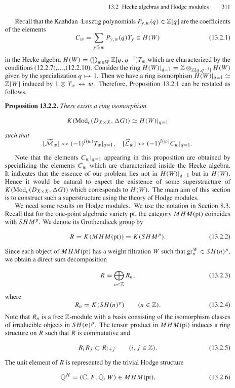
13.2 Hecke algebras and Hodge modules 311
Recall that the Kazhdan–Lusztig polynomials Py,w(q) ∈ Z[q] are the coefficientsof the elements
Cw =∑y�w
Py,w(q)Ty ∈ H(W) (13.2.1)
in the Hecke algebra H(W) = ⊕w∈W Z[q, q−1]Tw which are characterized by the
conditions (12.2.7),…,(12.2.10). Consider the ring H(W)|q=1 = Z ⊗Z[q,q−1] H(W)
given by the specialization q �→ 1. Then we have a ring isomorphism H(W)|q=1 �Z[W ] induced by 1 ⊗ Tw ↔ w. Therefore, Proposition 13.2.1 can be restated asfollows.
Proposition 13.2.2. There exists a ring isomorphism
K(Modc(DX×X, �G)) � H(W)|q=1
such that[Mw] ↔ (−1)l(w)Tw|q=1, [Lw] ↔ (−1)l(w)Cw|q=1.
Note that the elements Cw|q=1 appearing in this proposition are obtained byspecializing the elements Cw which are characterized inside the Hecke algebra.It indicates that the essence of our problem lies not in H(W)|q=1 but in H(W).Hence it would be natural to expect the existence of some superstructure ofK(Modc(DX×X, �G)) which corresponds to H(W). The main aim of this sectionis to construct such a superstructure using the theory of Hodge modules.
We need some results on Hodge modules. We use the notation in Section 8.3.Recall that for the one-point algebraic variety pt, the category MHM(pt) coincideswith SHMp. We denote its Grothendieck group by
R = K(MHM(pt)) = K(SHMp). (13.2.2)
Since each object of MHM(pt) has a weight filtration W such that grWn ∈ SH(n)p,
we obtain a direct sum decomposition
R =⊕n∈Z
Rn, (13.2.3)
whereRn = K(SH(n)p) (n ∈ Z). (13.2.4)
Note that Rn is a free Z-module with a basis consisting of the isomorphism classesof irreducible objects in SH(n)p. The tensor product in MHM(pt) induces a ringstructure on R such that R is commutative and
RiRj ⊂ Ri+j (i, j ∈ Z). (13.2.5)
The unit element of R is represented by the trivial Hodge structure
QH = (C, F, Q, W) ∈ MHM(pt), (13.2.6)

312 13 Hecke Algebras and Hodge Modules
grFp = 0 (p = 0), grW
n = 0 (n = 0).
Furthermore, the dualizing functor in MHM(pt) induces an involution r �→ r of thering R with the property
Ri = R−i (i ∈ Z). (13.2.7)
Finally, consider an injective homomorphism Z[q, q−1] ↪→ R of rings defined byqn �→ [QH (−n)]. Then we have
q ∈ R2, q = q−1. (13.2.8)
Now let Y be a smooth algebraic variety endowed with an action of an algebraicgroup K . Then the notion of K-equivariant mixed Hodge modules on Y can bedefined similarly to the case of K-equivariant DY -modules because we also haveinverse image functors in the category of mixed Hodge modules. We denote theabelian category of K-equivariant mixed Hodge modules on Y by MHM(Y, K). ItsGrothendieck group is denoted by K(MHM(Y, K)). By the tensor product functor
MHM(pt) × MHM(Y, K) → MHM(Y, K) (13.2.9)
the Grothendieck group K(MHM(Y, K)) is naturally an R-module.Let us consider the case where Y consists of a single K-orbit. This is exactly the
case when Y is a homogeneous space K/K ′ for a closed subgroup K ′ of K . In thiscase we have the following equivalences of categories:
K-equivariant regular holonomic systems on Y∥∥K-equivariant regular connections on Y∣∣�K-equivariant C-local systems on Y an∣∣�
finite-dimensional representations of K ′/(K ′)0 over C
Therefore, Modc(DY , K) = Modrh(DY , K) is equivalent to the category of finite-dimensional representations of the finite group K ′/(K ′)0 over C. In the case of Hodgemodules the situation is more complicated, because Q-structures and filtrations areconcerned. However, as in the case of D-modules the next proposition holds.
Proposition 13.2.3. Assume that Y is a homogeneous space K/K ′ of an algebraicgroup K . Then we have
MHM(Y, K) � MHM(pt, K ′/(K ′)0).
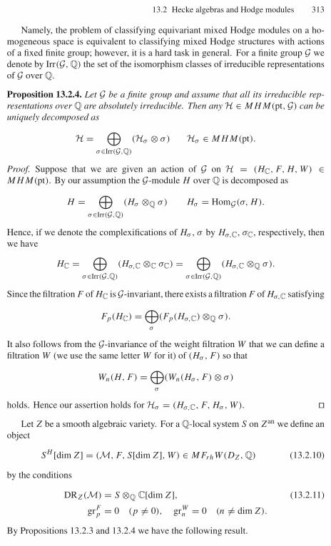
13.2 Hecke algebras and Hodge modules 313
Namely, the problem of classifying equivariant mixed Hodge modules on a ho-mogeneous space is equivalent to classifying mixed Hodge structures with actionsof a fixed finite group; however, it is a hard task in general. For a finite group G wedenote by Irr(G, Q) the set of the isomorphism classes of irreducible representationsof G over Q.
Proposition 13.2.4. Let G be a finite group and assume that all its irreducible rep-resentations over Q are absolutely irreducible. Then any H ∈ MHM(pt, G) can beuniquely decomposed as
H =⊕
σ∈Irr(G,Q)
(Hσ ⊗ σ) Hσ ∈ MHM(pt).
Proof. Suppose that we are given an action of G on H = (HC, F, H, W) ∈MHM(pt). By our assumption the G-module H over Q is decomposed as
H =⊕
σ∈Irr(G,Q)
(Hσ ⊗Q σ) Hσ = HomG(σ, H).
Hence, if we denote the complexifications of Hσ , σ by Hσ,C, σC, respectively, thenwe have
HC =⊕
σ∈Irr(G,Q)
(Hσ,C ⊗C σC) =⊕
σ∈Irr(G,Q)
(Hσ,C ⊗Q σ).
Since the filtration F of HC is G-invariant, there exists a filtration F of Hσ,C satisfying
Fp(HC) =⊕
σ
(Fp(Hσ,C) ⊗Q σ).
It also follows from the G-invariance of the weight filtration W that we can define afiltration W (we use the same letter W for it) of (Hσ , F ) so that
Wn(H, F ) =⊕
σ
(Wn(Hσ , F ) ⊗ σ)
holds. Hence our assertion holds for Hσ = (Hσ,C, F, Hσ , W). ��Let Z be a smooth algebraic variety. For a Q-local system S on Zan we define an
object
SH [dim Z] = (M, F, S[dim Z], W) ∈ MFrhW(DZ, Q) (13.2.10)
by the conditions
DRZ(M) = S ⊗Q C[dim Z], (13.2.11)
grFp = 0 (p = 0), grW
n = 0 (n = dim Z).
By Propositions 13.2.3 and 13.2.4 we have the following result.
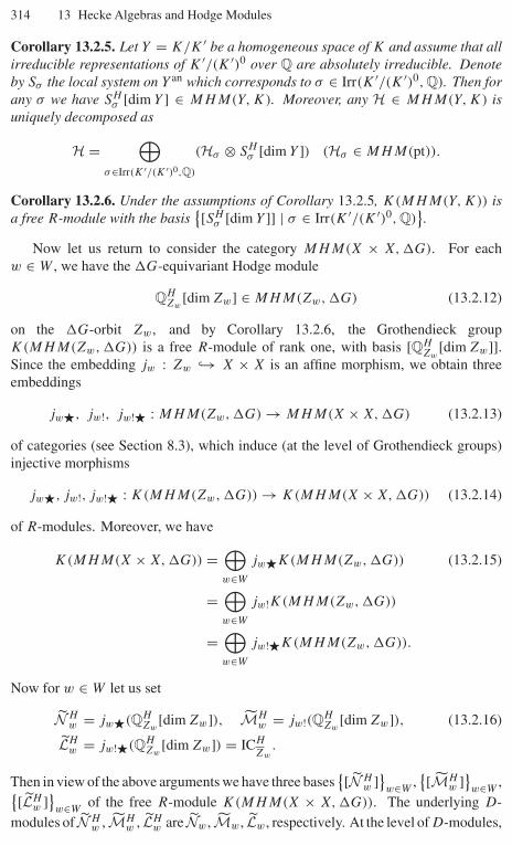
314 13 Hecke Algebras and Hodge Modules
Corollary 13.2.5. Let Y = K/K ′ be a homogeneous space of K and assume that allirreducible representations of K ′/(K ′)0 over Q are absolutely irreducible. Denoteby Sσ the local system on Y an which corresponds to σ ∈ Irr(K ′/(K ′)0, Q). Then forany σ we have SH
σ [dim Y ] ∈ MHM(Y, K). Moreover, any H ∈ MHM(Y, K) isuniquely decomposed as
H =⊕
σ∈Irr(K ′/(K ′)0,Q)
(Hσ ⊗ SHσ [dim Y ]) (Hσ ∈ MHM(pt)).
Corollary 13.2.6. Under the assumptions of Corollary 13.2.5, K(MHM(Y, K)) isa free R-module with the basis
{[SHσ [dim Y ]] | σ ∈ Irr(K ′/(K ′)0, Q)
}.
Now let us return to consider the category MHM(X × X, �G). For eachw ∈ W , we have the �G-equivariant Hodge module
QHZw
[dim Zw] ∈ MHM(Zw, �G) (13.2.12)
on the �G-orbit Zw, and by Corollary 13.2.6, the Grothendieck groupK(MHM(Zw, �G)) is a free R-module of rank one, with basis [QH
Zw[dim Zw]].
Since the embedding jw : Zw ↪→ X × X is an affine morphism, we obtain threeembeddings
jw�, jw!, jw!� : MHM(Zw, �G) → MHM(X × X, �G) (13.2.13)
of categories (see Section 8.3), which induce (at the level of Grothendieck groups)injective morphisms
jw�, jw!, jw!� : K(MHM(Zw, �G)) → K(MHM(X × X, �G)) (13.2.14)
of R-modules. Moreover, we have
K(MHM(X × X, �G)) =⊕w∈W
jw�K(MHM(Zw, �G)) (13.2.15)
=⊕w∈W
jw!K(MHM(Zw, �G))
=⊕w∈W
jw!�K(MHM(Zw, �G)).
Now for w ∈ W let us set
N Hw = jw�(QH
Zw[dim Zw]), MH
w = jw!(QHZw
[dim Zw]), (13.2.16)
LHw = jw!�(QH
Zw[dim Zw]) = ICH
Zw.
Then in view of the above arguments we have three bases{[N H
w ]}w∈W
,{[MH
w ]}w∈W
,{[LHw ]}
w∈Wof the free R-module K(MHM(X × X, �G)). The underlying D-
modules of N Hw , MH
w , LHw are Nw, Mw, Lw, respectively. At the level of D-modules,
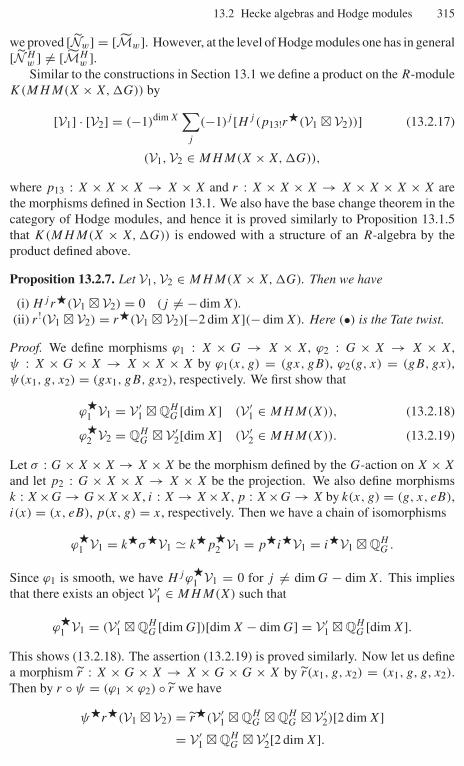
13.2 Hecke algebras and Hodge modules 315
we proved [Nw] = [Mw]. However, at the level of Hodge modules one has in general[N H
w ] = [MHw ].
Similar to the constructions in Section 13.1 we define a product on the R-moduleK(MHM(X × X, �G)) by
[V1] · [V2] = (−1)dim X∑
j
(−1)j [Hj (p13!r�(V1 � V2))] (13.2.17)
(V1, V2 ∈ MHM(X × X, �G)),
where p13 : X × X × X → X × X and r : X × X × X → X × X × X × X arethe morphisms defined in Section 13.1. We also have the base change theorem in thecategory of Hodge modules, and hence it is proved similarly to Proposition 13.1.5that K(MHM(X × X, �G)) is endowed with a structure of an R-algebra by theproduct defined above.
Proposition 13.2.7. Let V1, V2 ∈ MHM(X × X, �G). Then we have
(i) Hj r�(V1 � V2) = 0 (j = − dim X).(ii) r !(V1 � V2) = r�(V1 � V2)[−2 dim X](− dim X). Here (•) is the Tate twist.
Proof. We define morphisms ϕ1 : X × G → X × X, ϕ2 : G × X → X × X,ψ : X × G × X → X × X × X by ϕ1(x, g) = (gx, gB), ϕ2(g, x) = (gB, gx),ψ(x1, g, x2) = (gx1, gB, gx2), respectively. We first show that
ϕ�1 V1 = V ′
1 � QHG [dim X] (V ′
1 ∈ MHM(X)), (13.2.18)
ϕ�2 V2 = QH
G � V ′2[dim X] (V ′
2 ∈ MHM(X)). (13.2.19)
Let σ : G × X × X → X × X be the morphism defined by the G-action on X × X
and let p2 : G × X × X → X × X be the projection. We also define morphismsk : X×G → G×X×X, i : X → X×X, p : X×G → X by k(x, g) = (g, x, eB),i(x) = (x, eB), p(x, g) = x, respectively. Then we have a chain of isomorphisms
ϕ�1 V1 = k�σ�V1 � k�p
�2 V1 = p�i�V1 = i�V1 � QH
G.
Since ϕ1 is smooth, we have Hj ϕ�1 V1 = 0 for j = dim G − dim X. This implies
that there exists an object V ′1 ∈ MHM(X) such that
ϕ�1 V1 = (V ′
1 � QHG [dim G])[dim X − dim G] = V ′
1 � QHG [dim X].
This shows (13.2.18). The assertion (13.2.19) is proved similarly. Now let us definea morphism r : X × G × X → X × G × G × X by r(x1, g, x2) = (x1, g, g, x2).Then by r ◦ ψ = (ϕ1 × ϕ2) ◦ r we have
ψ�r�(V1 � V2) = r�(V ′1 � QH
G � QHG � V ′
2)[2 dim X]= V ′
1 � QHG � V ′
2[2 dim X].
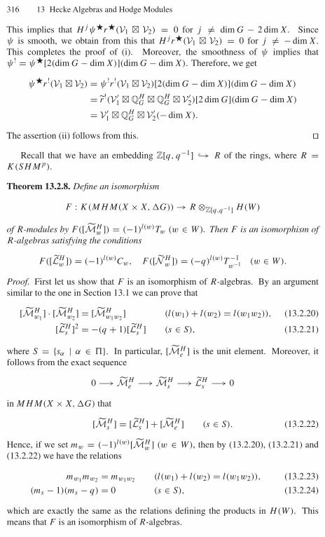
316 13 Hecke Algebras and Hodge Modules
This implies that Hj ψ�r�(V1 � V2) = 0 for j = dim G − 2 dim X. Sinceψ is smooth, we obtain from this that Hj r�(V1 � V2) = 0 for j = − dim X.This completes the proof of (i). Moreover, the smoothness of ψ implies thatψ ! = ψ�[2(dim G − dim X)](dim G − dim X). Therefore, we get
ψ�r !(V1 � V2) = ψ !r !(V1 � V2)[2(dim G − dim X)](dim G − dim X)
= r !(V ′1 � QH
G � QHG � V ′
2)[2 dim G](dim G − dim X)
= V ′1 � QH
G � V ′2(− dim X).
The assertion (ii) follows from this. ��Recall that we have an embedding Z[q, q−1] ↪→ R of the rings, where R =
K(SHMp).
Theorem 13.2.8. Define an isomorphism
F : K(MHM(X × X, �G)) → R ⊗Z[q,q−1] H(W)
of R-modules by F([MHw ]) = (−1)l(w)Tw (w ∈ W). Then F is an isomorphism of
R-algebras satisfying the conditions
F([LHw ]) = (−1)l(w)Cw, F ([N H
w ]) = (−q)l(w)T −1w−1 (w ∈ W).
Proof. First let us show that F is an isomorphism of R-algebras. By an argumentsimilar to the one in Section 13.1 we can prove that
[MHw1
] · [MHw2
] = [MHw1w2
] (l(w1) + l(w2) = l(w1w2)), (13.2.20)
[LHs ]2 = −(q + 1)[LH
s ] (s ∈ S), (13.2.21)
where S = {sα | α ∈ $}. In particular, [MHe ] is the unit element. Moreover, it
follows from the exact sequence
0 −→ MHe −→ MH
s −→ LHs −→ 0
in MHM(X × X, �G) that
[MHs ] = [LH
s ] + [MHe ] (s ∈ S). (13.2.22)
Hence, if we set mw = (−1)l(w)[MHw ] (w ∈ W), then by (13.2.20), (13.2.21) and
(13.2.22) we have the relations
mw1mw2 = mw1w2 (l(w1) + l(w2) = l(w1w2)), (13.2.23)
(ms − 1)(ms − q) = 0 (s ∈ S), (13.2.24)
which are exactly the same as the relations defining the products in H(W). Thismeans that F is an isomorphism of R-algebras.
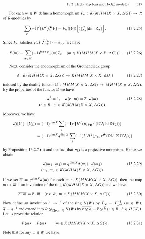
13.2 Hecke algebras and Hodge modules 317
For each w ∈ W define a homomorphism Fw : K(MHM(X × X, �G)) → R
of R-modules by∑k
(−1)k[Hkj�w V] = Fw([V])
[QH
Zw[dim Zw]
]. (13.2.25)
Since Fw satisfies Fw([MHy ]) = δy,w we have
F(m) =∑w∈W
(−1)l(w)Fw(m)Tw (m ∈ K(MHM(X × X, �G))). (13.2.26)
Next, consider the endomorphism of the Grothendieck group
d : K(MHM(X × X, �G)) → K(MHM(X × X, �G)) (13.2.27)
induced by the duality functor D : MHM(X × X, �G) → MHM(X × X, �G).By the properties of the functor D we have
d2 = 1, d(r · m) = r · d(m) (13.2.28)
(r ∈ R, m ∈ K(MHM(X × X, �G))).
Moreover, we have
d([V1] · [V2]) = (−1)dim X∑
j
(−1)j [Hj (p13�r !(DV1 � DV2))]
= (−1)dim Xqdim X∑
j
(−1)j [Hj (p13!r�(DV1 � DV2))]
by Proposition 13.2.7 (ii) and the fact that p13 is a projective morphism. Hence weobtain
d(m1 · m2) = qdim Xd(m1) · d(m2) (13.2.29)
(m1, m2 ∈ K(MHM(X × X, �G))).
If we set m = qdim Xd(m) for each m ∈ K(MHM(X × X, �G)), then the mapm �→ m is an involution of the ring K(MHM(X × X, �G)) and we have
r · m = r · m (r ∈ R, m ∈ K(MHM(X × X, �G))). (13.2.30)
Now define an involution h �→ h of the ring H(W) by T w = T −1w−1 (w ∈ W),
q = q−1 and extend it to R ⊗Z[q,q−1] H(W) by r ⊗ h = r ⊗ h (r ∈ R, h ∈ H(W)).Let us prove the relation
F(m) = F(m) (m ∈ K(MHM(X × X, �G))). (13.2.31)
Note that for any w ∈ W we have
318 13 Hecke Algebras and Hodge Modules
DLHw = LH
w (dim X + l(w)). (13.2.32)
Let us consider the special case of w = s ∈ S. Then it follows from (13.2.24) that
F(ms) = q−1Ts + (q−1 − 1) = T −1s = F(ms). (13.2.33)
Since K(Mod(X × X, �G)) is generated by the elements {ms}s∈S as an R-module,we see from this that (13.2.31) holds.
Now we can prove the remaining assertions. The proof of F([N Hw ]) =
(−q)l(w)T −1w−1 is easy. It follows immediately from N H
w = (DMHw )(− dim X−l(w))
and (13.2.31). So let us calculate F([LHw ]). First set
C′w = (−1)l(w)F ([LH
w ]) =∑y�w
P ′y,wTy (P ′
y,w ∈ R). (13.2.34)
Then we have
C′w = ql(w)C′
w, (13.2.35)
P ′w,w = 1, (13.2.36)
P ′y,w ∈
⊕i�l(w)−l(y)−1
Ri for y < w. (13.2.37)
Here (13.2.35) follows from (13.2.32). By the definition of LHw (13.2.36) is also clear.
Let us prove (13.2.37). Note that Hkj�y LH
w has mixed weights � dim Zw+k becauseLH
w has a pure weight dim Zw. Moreover, by a property of intersection cohomology
complexes, we have Hkj�y LH
w = 0 for any k � 0. Therefore, if Hkj�y LH
w = 0,then it has mixed weights < dim Zw. On the other hand, by (13.2.26) we have
(−1)l(w)−l(y)∑
k
(−1)k[Hkj�y LH
w ] = P ′y,w
[QH
Zy[dim Zy]
]. (13.2.38)
Since QHZy
[dim Zy] has the pure weight dim Zy , we obtain P ′y,w ∈ ⊕i<l(w)−l(y) Ri .
This shows (13.2.37). Using an argument completely similar to the one in [KL1],we can prove that the element C′
w ∈ R ⊗ H(W), satisfying the conditions (13.2.35),(13.2.36), (13.2.37), should be the same as Cw (we omit the details). Hence we getC′
w = Cw and F([LHw ]) = (−1)l(w)Cw. ��
We note that Proposition 13.2.1 follows from Theorem 13.2.8 by the specializationq �→ 1.
Finally, let us give a proof of Theorem 12.2.5 making use of the theory of Hodgemodules. The argument below is a faithful translation of the one in Kazhdan–Lusztig[KL2] which uses the theory of weights for étale sheaves in positive characteristicinstead of Hodge modules.
Proposition 13.2.9. If y � w, then Hkj�y LH
w has the pure weight dim Zw + k.
13.2 Hecke algebras and Hodge modules 319
In order to prove this we need the following.
Lemma 13.2.10. For a1, . . . , aN ∈ N+ define an action of C× on CN by
z · (x1, . . . , xN) = (za1x1, . . . , zaN xN).
Let Z be a C×-invariant irreducible closed subvariety of CN and set j : {0} ↪→ CN .Then j�(ICH
Z ) has the pure weight dim Z.
Proof. By a standard property of intersection cohomology complexes we have
Hkj�(ICHZ ) = 0 (k � 0). (13.2.39)
Since the origin 0 is the unique fixed point of the action of C× on Z, we also have that
Hkj�(ICHZ ) = Hk(CN, ICH
Z ). (13.2.40)
Therefore, it suffices to show that Hk(CN, ICHZ ) has the pure weight dim Z + k for
any k < 0. Set Z′ = Z \ {0}, and denote by i : CN \ {0} ↪→ CN the embedding.Then we have a distinguished triangle
j�j !(ICHZ ) −→ ICH
Z −→ i�(ICHZ′)
+1−→ .
Byj !(ICH
Z ) = Dj�D(ICHZ ) = Dj�(ICH
Z (dim Z))
we haveHk(j !(ICH
Z )) = (DH−k(j�(ICHZ )))(− dim Z).
Hence we obtain Hk(j !(ICHZ )) = 0 (k � 0) by (13.2.39). Therefore, it follows from
the distinguished triangle above that
Hk(CN, ICHZ )
∼−→ Hk(CN \ {0}, ICHZ′) (k < 0).
Now it remains to prove that Hk(CN \ {0}, ICHZ′) has the pure weight dim Z + k for
k < 0.By the assumption on the action of C× there exists a geometric quotients P =
(CN \ {0})/C×, Z′′ = Z′/C× of CN \ {0}, Z′, respectively. Then Z′′ is a closedsubvariety of the projective variety P . Let ϕ : CN \ {0} → P be the canonicalquotient morphism with respect to the C×-action. By ICH
Z′ = ϕ�ICHZ′′ [1] we have a
distinguished triangle
ICHZ′′ [−1](−1) −→ ICH
Z′′ [1] −→ ϕ�ICHZ′
+1−→ .
From this we obtain a cohomology long exact sequence
· · · −→ Hk−1(P, ICHZ′′)(−1)
ψk−→ Hk+1(P, ICHZ′′)
−→ Hk(CN \ {0}, ICHZ′) −→ · · · .
By the hard Lefschetz theorem for Hodge modules, the homomorphism ψk is injectivefor k � 0. Therefore, for k < 0, Hk(CN \ {0}, ICH
Z′) is a quotient of Hk+1(P, ICHZ′′).
The variety Z′′ being projective, Hk+1(P, ICHZ′′) and hence Hk(CN \{0}, ICH
Z′) musthave the pure weight dim Z′′ + k + 1 = dim Z + k. ��

320 13 Hecke Algebras and Hodge Modules
Proof of Proposition 13.2.9. Taking a suitable open subset U of X × X we have acommutative diagram
Zy ∩ U −→ Zw ∩ U −→ U
�∣∣ �∣∣ �∣∣{0} × CM −→ Z × CM −→ CN × CM,
where the horizontal arrows are embeddings. If we restrict the G-action on X×X to aone-dimensional torus in G, we can show that {0} ⊂ Z ⊂ CN satisfies the assumptionof Lemma 13.2.10. Hence the assertion follows from Lemma 13.2.10. ��Theorem 13.2.11. Suppose that y � w. We define integers cy,w,j ∈ Z by Py,w(q) =∑
j cy,w,j qj ∈ Z[q]. Then
(i) For k + l(w) − l(y) /∈ 2N we have Hkj�y (LH
w ) = 0.(ii) The integers cy,w,j ∈ Z are non-negative. Moreover, for k + l(w) − l(y) = 2j
(j � 0) we have an isomorphism
Hkj�y (LH
w ) = (QH
Zy[dim Zy])⊕cy,w,j .
Proof. By Proposition 13.2.9 we have an expression
Hkj�y (LH
w ) = Nk ⊗ QHZy
[dim Zy] (Nk ∈ SH(k + l(w) − l(y))p).
Therefore, by (13.2.38)∑k
(−1)l(w)+l(y)−k[Nk] =∑
j
cy,w,j qj .
Since we have [Nk] ∈ Rk+l(w)−l(y) and R = ⊕n Rn, q ∈ R2, we obtain
k + l(w) − l(y) = 2j + 1 =⇒ [Nk] = 0,
k + l(w) − l(y) = 2j =⇒ [Nk] = cy,w,j qj .
Hence our assertion follows from the fact that an object in SH(k)p is a direct sum offinitely many irreducible objects. ��
Now Theorem 12.2.5 is an immediate consequence of Theorem 13.2.11.
A
Algebraic Varieties
A.1 Basic definitions
Let k[X1, X2, . . . , Xn] be a polynomial algebra over an algebraically closed fieldk with n indeterminates X1, . . . , Xn. We sometimes abbreviate it as k[X] =k[X1, X2, . . . , Xn]. Let us associate to each polynomial f (X) ∈ k[X] its zero set
V (f ) := {x = (x1, x2, . . . , xn) ∈ kn | f (x) = f (x1, x2, . . . , xn) = 0}in the n-fold product set kn of k. For any subset S ⊂ k[X] we also set V (S) =⋂
f ∈S V (f ). Then we have the following properties:
(i) V (1) = ∅, V (0) = kn.(ii)
⋂i∈I V (Si) = V (
⋃i∈I Si).
(iii) V (S1) ∪ V (S2) = V (S1S2), where S1S2 := {fg | f ∈ S1, g ∈ S2}.The inclusion ⊂ of (iii) is clear. We will prove only the inclusion ⊃. For x ∈V (S1S2)\V (S2) there is an element g ∈ S2 such that g(x) = 0. On the other hand, itfollows from x ∈ V (S1S2) that f (x)g(x) = 0 (∀f ∈ S1). Hence f (x) = 0 (∀f ∈ S1)and x ∈ V (S1). So the part ⊃ was also proved.
By (i), (ii), (iii) the set kn is endowed with the structure of a topological spaceby taking {V (S) | S ⊂ k[X]} to be its closed subsets. We call this topology of kn
the Zariski topology. The closed subsets V (S) of kn with respect to it are calledalgebraic sets in kn. Note that V (S) = V (〈S〉), where 〈S〉 denotes the ideal of k[X]generated by S. Hence we may assume from the beginning that S is an ideal of k[X].Conversely, for a subset W ⊂ kn the set
I (W) := {f ∈ k[X] | f (x) = 0 (∀x ∈ W)
}is an ideal of k[X]. When W is a (Zariski) closed subset of kn, we have clearlyV (I (W)) = W . Namely, in the diagram
ideals in k[X] V
�I
closed subsets in kn
322 A Algebraic Varieties
we have V ◦I = Id. However, for an ideal J ⊂ k[X] the equality I (V (J )) = J doesnot hold in general. We have only I (V (J )) ⊃ J . The difference will be clarifiedlater by Hilbert’s Nullstellensatz.
Let V be a Zariski closed subset of kn (i.e., an algebraic set in kn). We regard it asa topological space by the relative topology induced from the Zariski topology of kn.We denote by k[V ] the k-algebra of k-valued functions on V obtained by restrictingpolynomial functions to V . It is called the coordinate ring of V . The restrictionmap ρV : k[X] → k[V ] given by ρV (f ) := f |V is a surjective homomorphism ofk-algebras with Ker ρV = I (V ), and hence we have k[V ] � k[X]/I (V ). For eachpoint x = (x1, x2, . . . , xn) ∈ kn of V define a homomorphism ex : k[V ] → k ofk-algebras by ex(f ) = f (x). Then we get a map
e : V −→ Homk-alg(k[V ], k) (x �−→ ex),
where Homk-alg(k[V ], k) denotes the set of the k-algebra homomorphisms fromk[V ] to k. Conversely, for a k-algebra homomorphism φ : k[V ] → k definex = (x1, x2, . . . , xn) ∈ kn by xi = φρV (Xi) (1 ≤ i ≤ n). Then we have x ∈ V andex = φ. Hence we have an identification V = Homk-alg(k[V ], k) as a set. Moreover,the closed subsets of V are of the form V (ρ−1
V (J )) = { x ∈ V | ex(J ) = 0 } ⊂ V forideals J of k[V ]. Therefore, the topological space V is recovered from the k-algebrak[V ]. It indicates the possibility of defining the notion of algebraic sets starting fromcertain k-algebras without using the embedding into kn. Note that the coordinate ringA = k[V ] is finitely generated over k, and reduced (i.e., does not contain non-zeronilpotent elements) because k[V ] is a subring of the ring of functions on V with valuesin the field k.
In this chapter we give an account of the classical theory of “algebraic varieties’’based on reduced finitely generated (commutative) algebras over algebraically closedfields (in the modern language of schemes one allows general commutative rings as“coordinate algebras’’).
The following two theorems are fundamental.
Theorem A.1.1 (Aweak form of Hilbert’Nullstellensatz). Any maximal ideal of thepolynomial ring k[X1, X2, . . . , Xn] is generated by the elements Xi −xi (1 ≤ i ≤ n)
for a point x = (x1, x2, . . . , xn) ∈ kn.
Theorem A.1.2 (Hilbert’s Nullstellensatz). We have I (V (J )) = √J , where
√J
is the radical { f ∈ k[X] | f N ∈ J for some N � 0} of J .
For the proofs, see, for example, [Mu]. ��For a finitely generated k-algebra A denote by Specm A the set of the maximal
ideals of A. For an algebraic set V ⊂ kn we have a bijection
Homk-alg(k[V ], k) � Specm k[V ] (e �−→ Ker e)
by TheoremA.1.1. Under this correspondence, the closed subsets in Specm k[V ] � V
are the setsV (I) = { m ∈ Specm k[V ] | m ⊃ I },

A.2 Affine varieties 323
where I ranges through the ideals of k[V ]. Theorem A.1.2 implies that there is a one-to-one correspondence between the closed subsets in Specm k[V ] and the radicalideals I (I = √
I ) of k[V ].
A.2 Affine varieties
Motivated by the arguments in the previous section, we start from a finitely generatedreduced commutative k-algebra A to define an algebraic variety. Namely, we setV = Specm A and define its topology so that the closed subsets are given by{
V (I) = {m ∈ Specm A | I ⊂ m} | I : ideals of A}.
By Hilbert’s Nullstellensatz (its weak form), we get the identification
V � Homk-alg(A, k).
We sometimes write a point x ∈ V as mx ∈ Specm A or ex ∈ Homk-alg(A, k). Underthis notation we have
f (x) = ex(f ) = (f mod mx) ∈ k
for f ∈ A. Here, we used the identification k � A/mx obtained by the compositeof the morphisms k ↪→ A → A/mx . Hence the ring A is regarded as a k-algebraconsisting of certain k-valued functions on V .
Recall that any open subset of V is of the form D(I) = V \ V (I), where I isan ideal of A. Since A is a noetherian ring (finitely generated over k), the ideal I isgenerated by a finite subset {f1, f2, . . . , fr} of I . Then we have
D(I) = V \( r⋂
i=1
V (fi))
=r⋃
i=1
D(fi),
where D(f ) = { x ∈ V | f (x) = 0 } = V \V (f ) for f ∈ A. We call an open subsetof the form D(f ) for f ∈ A a principal open subset of V . Principal open subsetsform a basis of the open subsets of V . Note that we have the equivalence
D(f ) ⊂ D(g) ⇐⇒ √(f ) ⊂ √
(g) ⇐⇒ f ∈ √(g)
by Hilbert’s Nullstellensatz.Assume that we are given an A-module M . We introduce a sheaf M on the
topological space V = Specm A as follows. For a multiplicatively closed subsetS of A we denote by S−1M the localization of M with respect to S. It consists ofthe equivalence classes with respect to the equivalence relation ∼ on the set of pairs(s, m) = m/s (s ∈ S, m ∈ M) given by m/s ∼ m′/s′ ⇐⇒ t (s′m − sm′) = 0(∃t ∈ S). By the ordinary operation rule of fractional numbers S−1A is endowedwith a ring structure and S−1M turns out to be an S−1A-module. For f ∈ A we set

324 A Algebraic Varieties
Mf = S−1f M , where Sf := {1, f, f 2, . . . }. Note that for two principal open subsets
D(f ) ⊂ D(g) a natural homomorphism rgf : Mg → Mf is defined as follows. We
have f n = hg (h ∈ A, n ∈ N), and then the element m/gl ∈ Mg is mapped tom/gl = hlm/hlgl = hlm/f nl ∈ Mf . In the case of D(f ) = D(g) we easily seeMf � Mg by considering the inverse.
Theorem A.2.1.(i) For an A-module M there exists a unique sheaf M on V = Specm A such that for
any principal open subset D(f ) we have M(D(f )) = Mf , and the restrictionhomomorphism M(D(f )) → M(D(g)) for D(f ) ⊂ D(g) is given by r
gf .
(ii) The sheaf OV := A is naturally a sheaf of k-algebras on V .(iii) For an A-module M the sheaf M is naturally a sheaf of OV -module. The stalk
of M at x ∈ V is given by
Mmx = (A � mx)−1M = lim−→f (x)=0
Mf .
This is a module over the local ring OV,x := Amx = (A � mx)−1A.
The key point of the proof is the fact that the functor D(f ) �→ Mf on the categoryof principal open subsets {D(f ) | f ∈ A} satisfies the “axioms of sheaves (for a basisof open subsets),’’ which is assured by the next lemma.
Lemma A.2.2. Assume that the condition 〈f1, f2, . . . , fr 〉 1 is satisfied in the ringA. Then for an A-module M we have an exact sequence
0 −→ Mα−→
r∏i=1
Mfi
β−→∏i,j
Mfifj,
where the last arrow maps (si)ri=1 to si − sj ∈ Mfifj
(1 ≤ i, j ≤ r).
Proof. We first show that for any N ∈ N there exists g1, . . . , gr satisfying∑
i gifNi =
1. Note that our assumption 〈f1, f2, . . . , fr 〉 1 is equivalent to saying that for anym ∈ Specm A there exists at least one element fi such that fi /∈ m (Specm A =⋃r
i=1 D(fi)). If fi /∈ m, then we have f Ni /∈ m for any N since m is a prime ideal.
Therefore, we get 〈f N1 , f N
2 , . . . , f Nr 〉 1, and the assertion is proved.
Let us show the injectivity of α. Assume m ∈ Ker α. Then there exists N � 0such that f N
i m = 0 (1 ≤ i ≤ r). Combining it with the equality∑
i gifNi = 1 we
get m = ∑i gif
Ni m = 0.
Next assume that (ml) ∈ ∏l Mfl∈ Ker β. We will show that there is an element
m ∈ M such that α(m) = (ml). It follows from our assumption that mi = mj inMfifj
(1 ≤ i, j ≤ r). This is equivalent to saying that (fifj )N(mi − mj ) = 0(1 ≤ i, j ≤ r) for a large number N . That is, f N
j f Ni mi = f N
i f Nj mj . Now
set m = ∑ri=1 gi(f
Ni mi) (
∑gif
Ni = 1). Then for any 1 ≤ l ≤ r we have
f Nl m = f N
l
∑i gi(f
Ni mi) = ∑
i gifNi (f N
l mi) = ∑i gif
Ni f N
l ml = f Nl ml and
f Nl (m − ml) = 0. Hence we have α(m) = (ml). ��

A.3 Algebraic varieties 325
For a general open subset U = ⋃ri=1 D(fi) of U we have
�(U, M) = {(si) ∈ Mfi
| si = sj in Mfifj(1 ≤ i, j ≤ r)
}.
In particular, for OV = A we have
�(U, OV ) = {f : U → k | for each point of U,
there is an open neighborhood D(g) such that f |D(g) ∈ Ag.}Let (X, OX) be a pair of a topological space X and a sheaf OX of k-algebras on
X consisting of certain k-valued functions. We say that the pair (X, OX) (or simplyX) is an affine variety if (X, OX) is isomorphic to some (V , OV ) (V = Specm A,
OV = A) in the sense that there exists a homeomorphism φ : X −→∼ V such that
the correspondence f �→ f ◦ φ gives an isomorphism �(φ(U), OV ) −→∼ �(U, OX)
for any open subset U of V . In this case we have a natural isomorphism φ� :φ−1OV −→∼ OX of a sheaf of k-algebras. In particular, we have an isomorphism
φ�x : OV,φ(x) −→∼ OX,x of local rings for any x ∈ X.
A.3 Algebraic varieties
Let (X, OX) be a pair of a topological space X and a sheaf OX of k-algebras consistingof certain k-valued functions. We say that the pair (X, OX) (or simply X) is called aprevariety over k if it is locally an affine variety (i.e., if for any point x ∈ X there is anopen neighborhood U x such that (U, OX|U ) is isomorphic to an affine variety).In such cases, we call the sheaf OX the structure sheaf of X and sections of OX arecalled regular functions. A morphism φ : X → Y between prevarieties X, Y is acontinuous map so that for any open subset U of Y and any f ∈ �(U, OY ) we havef ◦ φ ∈ �(f −1U, OX).
A prevariety X is called an algebraic variety if it is quasi-compact and separated .Let us explain more precisely these two conditions.
The quasi-compactness is a purely topological condition. We say that a topologicalspace X is quasi-compact if any open covering of X admits a finite subcovering. Wesay “quasi’’ because X is not assumed to be Hausdorff. In fact, an algebraic varietyis not Hausdorff unless it consists of finitely many points. In particular, an algebraicvariety X is covered by finitely many affine varieties.
The condition of separatedness plays an alternative role to that of the Hausdorffcondition. To define it we need the notion of products of prevarieties.
We define the product V1 × V2 of two affine varieties V1, V2 to be the affinevariety associated to the tensor product A1 ⊗k A2 (Ai = �(Vi, OVi
)) of k-algebras.This operation is possible thanks to the following proposition.
Proposition A.3.1. For any pair A1, A2 of finitely generated reduced k-algebras thetensor product A1 ⊗k A2 is also reduced.
326 A Algebraic Varieties
Proof. Consider the embeddings Vi ⊂ Ani (i = 1, 2) and V1 × V2 ⊂ An1+n2 . Next,define the ring k[V1 × V2] to be the restriction of the polynomial ring k[An1+n2 ] toV1 × V2. Then the restriction map ϕ : k[V1] ⊗k k[V2] → k[V1 × V2] is bijective (theright-hand side is obviously reduced). The surjectivity is clear. We can also provethe injectivity, observing that for any linearly independent elements {fi} (resp. {gj })in k[V1] (resp. k[V2]) over k the elements {ϕ(figj )} are again linearly independentin k[V1 × V2]. ��
By definition the product V1 × V2 of affine varieties V1, V2 has a finer topologythan the usual product topology.
Now let us give the definition of the product of two prevarieties X, Y . LetX = ⋃
i Vi , Y = ⋃j Uj be affine open coverings of X and Y , respectively. Then the
product set X×Y is covered by { Vi ×Uj }(i,j) (X×Y = ⋃(i,j) Vi ×Uj ). Note that we
regard the product sets Vi×Uj as affine varieties by the above arguments. Namely, thestructure sheaf OVi×Uj
is associated to the tensor product �(Vi, OVi)⊗k�(Uj , OUj
).Then we can glue (Vi × Uj , OVi×Uj
) to get a topology of X×Y and a sheaf OX×Y ofk-algebras consisting of certain k-valued functions on X×Y , for which (X×Y, OX×Y )
is a prevariety. This prevariety is called the product of two prevarieties X and Y . Itis the “fiber product’’ in the category of prevarieties.
Using these definitions, we say that a prevariety X is separated if the diagonalset � = {(x, x) ∈ X × X} is closed in the self-product X × X.
Let us add some remarks.
(i) If φ : X → Y is a morphism of algebraic varieties, then its graph �φ ={ (x, φ(x)) ∈ X × Y } is a closed subset of X × Y .
(ii) Affine varieties are separated (hence they are algebraic varieties).
A.4 Quasi-coherent sheaves
Let (X, OX) be an algebraic variety. We say that a sheaf F of OX-module (hereafter,we simply call F an OX-module) is quasi-coherent over OX if for each point x ∈ X
there exists an affine open neighborhood V x and a module MV over AV = OX(V )
such that F |V � MV as OV -modules (MV is an OV -module on V = Specm AV
constructed from the AV -module MV by Theorem A.2.1). If, moreover, every MV isfinitely generated over AV , we say that F is coherent over OX. The next theorem isfundamental.
Theorem A.4.1.(i) (Chevalley) The following conditions on an algebraic variety X are equivalent:
(a) X is an affine variety.(b) For any quasi-coherent OX-module F we have Hi(X, F ) = 0 (i ≥ 1).(c) For any quasi-coherent OX-module F we have H 1(X, F ) = 0.
(ii) Let X be an affine variety and A = OX(X) its coordinate ring. Then the functor
Mod(A) M �−→ M ∈ Modqc(OX)
A.4 Quasi-coherent sheaves 327
from the category Mod(A) of A-modules to the category Modqc(OX) of quasi-coherent OX-modules induces an equivalence of categories. Namely, any quasi-coherent OX-module is isomorphic to the sheaf M constructed from an A-moduleM , and there exists an isomorphism
HomA(M, N) −→∼ HomOX(M, N).
In particular, for a quasi-coherent OX-module F we have
F � F (X).
By Theorem A.4.1 (ii) local properties of a quasi-coherent OX-module F canbe deduced from those of the OX(V )-module F(V ) for an affine neighborhood V .For example, F is locally free (resp. coherent) if and only if every point x ∈ X
has an affine open neighborhood V such that F(V ) is free (resp. finitely generated)over OX(V ).
Let us give some examples.
Example A.4.2. Tangent sheaf �X and cotangent sheaf �1X (In this book, �X stands
for the sheaf �nX := ∧n
�1X (n = dim X) of differential forms of top degree). We
denote by EndkOX the sheaf of k-linear endomorphisms of OX. We say that a sectionθ ∈ (EndkOX)(X) is a vector field on X if for each open subset U ⊂ X the restrictionθ(U) := θ |U ∈ (EndkOX)(U) satisfies the condition
θ(U)(fg) = θ(U)(f )g + f θ(U)(g) (f, g ∈ OX(U)).
For an open subset U of X, denote the set of the vector fields θ (∈ (EndkOU )(U)) onU by �(U). Then �(U) is an OX(U)-module, and the presheaf U �→ �(U) turnsout to be a sheaf (of OX-modules). We denote this sheaf by �X and call it the tangent
sheaf of X. When U is affine, we have �U � Derk(A) for A = OX(U), where theright-hand side is the OU -module associated to the A-module
Derk(A) := { θ ∈ Endk A | θ(fg) = θ(f )g + f θ(g) (f, g ∈ A) }of the derivations of A over k. It follows from this fact that �X is a coherent OX-module. Indeed, if A = k[X]/I (here k[X] = k[X1, X2, . . . , Xn] is a polynomialring), then we have
Derk(k[X]) =n⊕
i=1
k[X]∂i
(∂i := ∂
∂Xi
)(free k[X]-module of rank n) and
Derk(A) � {θ ∈ Derk(k[X]) | θ(I ) ⊂ I }.Hence Derk(A) is finitely generated over A.

328 A Algebraic Varieties
On the other hand we define the cotangent sheaf of X by �1X := δ−1(J /J 2),
where δ : X → X × X is the diagonal embedding, J is the ideal sheaf of δ(X) inX × X defined by
J (V ) = {f ∈ OX×X(V ) | f (V ∩ δ(X)) = {0}}for any open subset V of X×X, and δ−1 stands for the sheaf-theoretical inverse imagefunctor. Sections of the sheaf �1
X are called differential forms. By the canonicalmorphism OX → δ−1OX×X of sheaf of k-algebras �1
X is naturally an OX-module.We have a morphism d : OX → �1
X of OX-modules defined by df = f ⊗ 1 −1 ⊗ f mod δ−1J 2. It satisfies d(fg) = d(f )g + f (dg) for any f, g ∈ OX.For α ∈ HomOX
(�1X, OX) we have α ◦ d ∈ �X, which gives an isomorphism
HomOX(�1
X, OX) � �X of OX-modules.
A.5 Smoothness, dimensions and local coordinate systems
Let x be a point of an algebraic variety X. We say that X is smooth (or non-singular)at x ∈ X if the stalk OX,x is a regular local ring. This condition is satisfied if andonly if the cotangent sheaf �1
X is a free OX-module on an open neighborhood of x.The smooth points of X form an open subset of X. Let us denote this open subset byXreg. An algebraic variety is called smooth (or non-singular) if all of its points aresmooth. It is equivalent to saying that �1
X is a locally free OX-module. In this case�X is also locally free of the same rank by HomOX
(�1X, OX) � �X. For a smooth
point x ∈ X the dimension of X at x is defined by
dimx X := rankOX,x�X,x = rankOX,x
�1X,x,
where �X,x and �1X,x are the stalks of �X and �1
X at x, respectively. It also coincideswith the Krull dimension of the regular local ring OX,x . We define the dimension ofX to be the locally constant function on Xreg defined by
(dim X)(x) := dimx X.
If X is irreducible, the value dimx X does not depend on the point x ∈ Xreg.
Theorem A.5.1. Let X be a smooth algebraic variety of dimension n. Then for eachpoint p ∈ X, there exist an affine open neighborhood V of p, regular functionsxi ∈ k[V ] = OX(V ), and vector fields ∂i ∈ �X(V ) (1 ≤ i ≤ n) satisfying theconditions {
[∂i, ∂j ] = 0, ∂i(xj ) = δij (1 ≤ i, j ≤ n)
�V = ⊕ni=1 OV ∂i .
Moreover, we can choose the functions x1, x2, . . . , xn so that they generate the max-imal ideal mp of the local ring OX,p at p.
A.5 Smoothness, dimensions and local coordinate systems 329
Proof. By the theory of regular local rings there exist n(= dimx X) functionsx1, . . . , xn ∈ mp generating the ideal mp. Then dx1, . . . , dxn is a basis of thefree OX,p-module �1
X,p. Hence we can take an affine open neighborhood V of
p such that �1X(V ) is a free module with basis dx1, . . . , dxn over OX(V ). Tak-
ing the dual basis ∂1, . . . , ∂n ∈ �X(V ) � HomOX(V )(�1X(V ), OX(V )) we get
∂i(xj ) = δij . Write [∂i, ∂j ] as [∂i, ∂j ] = ∑nl=1 gl
ij ∂l (glij ∈ OX(V )). Then we
have glij = [∂i, ∂j ] xl = ∂i∂j xl − ∂j ∂ixl = 0. Hence [∂i, ∂j ] = 0. ��
Definition A.5.2. The set { xi, ∂i | 1 ≤ i ≤ n } defined over an affine open neigh-borhood of p satisfying the conditions of Theorem A.5.1 is called a local coordinatesystem at p.
It is clear that this notion is a counterpart of the local coordinate system of acomplex manifold. Note that the local coordinate system {xi} defined on an affineopen subset V of a smooth algebraic variety does not necessarily separate the pointsin V . We only have an étale morphism V → kn given by q �→ (x1(q), . . . , xn(q)).
We have the following relative version of Theorem A.5.1.
Theorem A.5.3. Let Y be a smooth subvariety of a smooth algebraic variety X.Assume that dimp Y = m, dimp X = n at p ∈ Y . Then we can take an affine openneighborhood V of p in X and a local coordinate system {xi, ∂i | 1 ≤ i ≤ n} such thatY ∩V = {q ∈ V | xi(q) = 0 (m < i ≤ n)} (hence k[Y ∩V ] = k[V ]/∑i>m k[V ] xi)
and {xi, ∂i | 1 ≤ i ≤ m} is a local coordinate system of Y ∩ V . Here we regard∂i (1 ≤ i ≤ m) as derivations on k[Y ∩ V ] by using the relation ∂ixj = 0 (j > m).
Proof. The result follows from the fact that smooth ⇒ locally complete intersec-tion. ��
B
Derived Categories and Derived Functors
In this appendix, we give a brief account of the theory of derived categories withoutproofs. The basic references are Hartshorne [Ha1], Verdier [V2], Borel et al. [Bor3,Chapter 1], Gelfand–Manin [GeM], Kashiwara–Schapira [KS2], [KS4]. We espe-cially recommend the reader to consult Kashiwara–Schapira [KS4] for details on thissubject.
B.1 Motivation
The notion of derived categories is indispensable if one wants to fully understand thetheory of D-modules. Many operations of D-modules make sense only in derivedcategories, and the Riemann–Hilbert correspondence, which is the main subject ofPart I, cannot be formulated without this notion. Derived categories were introducedby A. Grothendieck [Ha1], [V2]. We hear that M. Sato arrived at the same notionindependently in his way of creating algebraic analysis. In this section we explainthe motivation of the theory of derived categories and give an outline of the theory.
Let us first recall the classical definition of right derived functors. Let C, C′ beabelian categories and F : C → C′ a left exact functor. Assume that the category Chas enough injectives, i.e., for any object X ∈ Ob(C) there exists a monomorphismX → I into an injective object I . Then for any X ∈ Ob(C) there exists an exactsequence
0 −→ X −→ I 0 −→ I 1 −→ · · ·such that I k is an injective object for any k ∈ Z. Such an exact sequence is called aninjective resolution of X. Next consider the complex
I˙ = [0 −→ I 0 −→ I 1 −→ I 2 −→ I 3 · · · ]
in C and apply to it the functor F . Then we obtain a complex
F(I˙) = [0 −→ F(I 0) −→ F(I 1) −→ F(I 2) −→ F(I 3) · · · ]
in C′. As is well known in homological algebra the nth cohomology group of F(I˙):

332 B Derived Categories and Derived Functors
HnF(I˙) = Ker[F(In) −→ F(In+1)]/ Im[F(In−1) −→ F(In)]does not depend on the choice of injective resolutions, and is uniquely determined upto isomorphisms. Set RnF(X) = HnF(I˙) ∈ Ob(C′). Then RnF defines a functorRnF : C → C′. We call RnF the nth derived functor of F . For n < 0 we haveRnF = 0 and R0F = F . Similar construction can be applied also to complexes in Cwhich are bounded below. Indeed, consider a complex
X˙ = [ · · · −→ 0 −→ 0 −→ Xk −→ Xk+1 −→ Xk+2 −→ · · · ]in C such that Xi = 0 for any i < k. Then there exists a complex
I˙ = [ · · · −→ 0 −→ 0 −→ I k −→ I k+1 −→ I k+2 −→ · · · ]of injective objects in C and a quasi-isomorphism f : X˙ → I , i.e., a morphism ofcomplexes f : X˙ → I˙ which induces an isomorphism Hi(X˙) � Hi(I˙) for anyi ∈ Z. We call I˙ an injective resolution of X . Since the injective resolution I˙and the complex F(I˙) are uniquely determined up to homotopy equivalences, thenth cohomology group HnF(I˙) ∈ Ob(C′) of F(I˙) is uniquely determined up toisomorphisms. Set RnF(X˙) = HnF(I˙) ∈ Ob(C′). If we introduce the homotopycategory K+(C) of complexes in C which are bounded below (for the definition seeSection B.2 below), this gives a functor RnF : K+(C) → C′. Such derived functorsfor “complexes’’ are frequently used in algebraic geometry.
However, this classical construction of derived functors has some defects. Sincewe treat only cohomology groups {HnF(I˙)}n∈Z of F(I˙), we lose various impor-tant information of the complex F(I˙) itself. Moreover, the above construction ofderived functors is not convenient for the composition of functors. For example, letG : C′ −→ C′′ be another left exact functor. Then, for X ∈ Ob(C) the equalityRi+j (G ◦ F)(X) = RiG(Rj F (X)) cannot be expected in general. The theory ofspectral sequences was invented as a remedy for such problems, but the best wayis to treat everything at the level of complexes without taking cohomology groups.Namely, we want to introduce certain categories of complexes and define a liftingRF (which will be also called a derived functor of F ) of RnF ’s between such cate-gories of complexes. This is the theory of derived categories. Indeed, the languageof derived categories allows one to formulate complicated relations among variousfunctors in a very beautiful and efficient way.
Now let us briefly explain the construction of derived categories. Let C(C) be thecategory of complexes in C. Since the injective resolutions f : X˙ → I˙ of X˙ are justquasi-isomorphisms in C(C), we should change the family of morphisms of C(C) sothat quasi-isomorphisms are isomorphisms in the new category. For this purpose weuse a general theory of localizations of categories (see Section B.4). However, thislocalization cannot be applied directly to the category C(C). So we first define thehomotopy category K(C) by making homotopy equivalences in C(C) invertible, andthen apply the localization. The derived category D(C) thus obtained is an additivecategory and not an abelian category any more. Therefore, we cannot consider shortexact sequences 0 → X˙ → Y˙ → Z˙ → 0 of complexes in D(C) as in C(C).
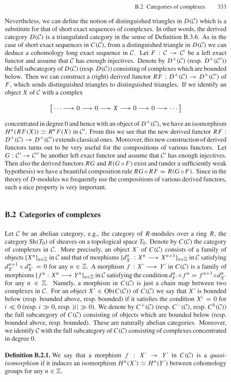
B.2 Categories of complexes 333
Nevertheless, we can define the notion of distinguished triangles in D(C) which is asubstitute for that of short exact sequences of complexes. In other words, the derivedcategory D(C) is a triangulated category in the sense of Definition B.3.6. As in thecase of short exact sequences in C(C), from a distinguished triangle in D(C) we candeduce a cohomology long exact sequence in C. Let F : C → C′ be a left exactfunctor and assume that C has enough injectives. Denote by D+(C) (resp. D+(C′))the full subcategory of D(C) (resp. D(C)) consisting of complexes which are boundedbelow. Then we can construct a (right) derived functor RF : D+(C) → D+(C′) ofF , which sends distinguished triangles to distinguished triangles. If we identify anobject X of C with a complex[ · · · −→ 0 −→ 0 −→ X −→ 0 −→ 0 −→ · · · ]concentrated in degree 0 and hence with an object of D+(C), we have an isomorphismHn(RF(X)) � RnF(X) in C′. From this we see that the new derived functor RF :D+(C) → D+(C′) extends classical ones. Moreover, this new construction of derivedfunctors turns out to be very useful for the compositions of various functors. LetG : C′ → C′′ be another left exact functor and assume that C′ has enough injectives.Then also the derived functors RG and R(G◦F) exist and (under a sufficiently weakhypothesis) we have a beautiful composition rule RG◦RF = R(G◦F). Since in thetheory of D-modules we frequently use the compositions of various derived functors,such a nice property is very important.
B.2 Categories of complexes
Let C be an abelian category, e.g., the category of R-modules over a ring R, thecategory Sh(T0) of sheaves on a topological space T0. Denote by C(C) the categoryof complexes in C. More precisely, an object X˙ of C(C) consists of a family ofobjects {Xn}n∈Z in C and that of morphisms {dn
X˙ : Xn −→ Xn+1}n∈Z in C satisfyingdn+1
X˙ ◦ dnX˙ = 0 for any n ∈ Z. A morphism f : X˙ −→ Y˙ in C(C) is a family of
morphisms {f n : Xn −→ Y n}n∈Z in C satisfying the condition dnY ˙ ◦f n = f n+1 ◦dn
X˙for any n ∈ Z. Namely, a morphism in C(C) is just a chain map between twocomplexes in C. For an object X˙ ∈ Ob(C(C)) of C(C) we say that X˙ is boundedbelow (resp. bounded above, resp. bounded) if it satisfies the condition Xi = 0 fori # 0 (resp. i � 0, resp. |i| � 0). We denote by C+(C) (resp. C−(C), resp. Cb(C))the full subcategory of C(C) consisting of objects which are bounded below (resp.bounded above, resp. bounded). These are naturally abelian categories. Moreover,we identify C with the full subcategory of C(C) consisting of complexes concentratedin degree 0.
Definition B.2.1. We say that a morphism f : X˙ → Y˙ in C(C) is a quasi-isomorphism if it induces an isomorphism Hn(X˙) � Hn(Y˙) between cohomologygroups for any n ∈ Z.
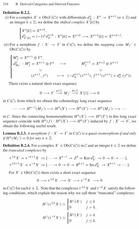
334 B Derived Categories and Derived Functors
Definition B.2.2.(i) For a complex X˙ ∈ Ob(C(C)) with differentials dn
X˙ : Xn → Xn+1 (n ∈ Z) andan integer k ∈ Z, we define the shifted complex X˙[k] by{
Xn[k] = Xn+k,
dnX˙[k] = (−1)kdn+k
X˙ : Xn[k] = Xn+k −→ Xn+1[k] = Xn+k+1.
(ii) For a morphism f : X˙ → Y˙ in C(C), we define the mapping cone Mf ˙ ∈Ob(C(C)) by⎧⎪⎪⎪⎪⎨⎪⎪⎪⎪⎩
Mnf = Xn+1 ⊕ Y n,
dnMf ˙ : Mn
f = Xn+1 ⊕ Y n −→ Mn+1f = Xn+2 ⊕ Y n+1
�� ��(xn+1, yn) �−→ (−dn+1
X˙ (xn+1), f n+1(xn+1) + dnY ˙(yn)).
There exists a natural short exact sequence
0 −→ Y˙ α(f )−→ Mf ˙ β(f )−→ X˙[1] −→ 0
in C(C), from which we obtain the cohomology long exact sequence
· · · −→ Hn−1(Mf ˙) −→ Hn(X˙) −→ Hn(Y˙) −→ Hn(Mf ˙) −→ · · ·in C. Since the connecting homomorphisms Hn(X˙) −→ Hn(Y˙) in this long exactsequence coincide with Hn(f ) : Hn(X˙) −→ Hn(Y˙) induced by f : X˙ → Y , weobtain the following useful result.
Lemma B.2.3. A morphism f : X˙ → Y˙ in C(C) is a quasi-isomorphism if and onlyif Hn(Mf ˙) = 0 for any n ∈ Z.
Definition B.2.4. For a complex X˙ ∈ Ob(C(C)) in C and an integer k ∈ Z we definethe truncated complexes by
τ�kX· = τ<k+1X· := [· · · → Xk−1 → Zk = Ker dkX˙ → 0 → 0 → · · · ],
τ�k+1X· = τ>kX· := [· · · → 0 → 0 → Bk+1 = Im dkX˙ → Xk+1 → · · · ].
For X˙ ∈ Ob(C(C)) there exists a short exact sequence
0 −→ τ�kX· −→ X· −→ τ>kX· −→ 0
in C(C) for each k ∈ Z. Note that the complexes τ�kX· and τ>kX· satisfy the follow-ing conditions, which explain the reason why we call them “truncated’’ complexes:
Hj (τ�kX·) �{
Hj (X·) j ≤ k
0 j > k,
Hj (τ>kX·) �{
Hj (X·) j > k
0 j ≤ k.
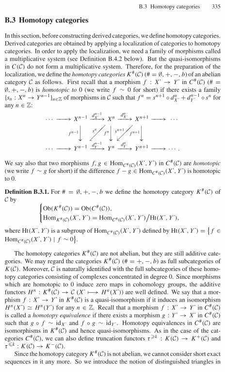
B.3 Homotopy categories 335
B.3 Homotopy categories
In this section, before constructing derived categories, we define homotopy categories.Derived categories are obtained by applying a localization of categories to homotopycategories. In order to apply the localization, we need a family of morphisms calleda multiplicative system (see Definition B.4.2 below). But the quasi-isomorphismsin C(C) do not form a multiplicative system. Therefore, for the preparation of thelocalization, we define the homotopy categories K#(C) (# = ∅, +, −, b) of an abeliancategory C as follows. First recall that a morphism f : X˙ → Y˙ in C#(C) (# =∅, +, −, b) is homotopic to 0 (we write f ∼ 0 for short) if there exists a family{sn : Xn → Y n−1}n∈Z of morphisms in C such that f n = sn+1 ◦ dn
X˙ + dn−1Y ˙ ◦ sn for
any n ∈ Z:
· · · −−−→ Xn−1 −−−→dn−1X˙ Xn −−−→dn
X˙ Xn+1 −−−→ · · ·⏐⏐⏐f n−1
���sn
⏐⏐⏐f n
���sn+1
⏐⏐⏐f n+1
· · · −−−→ Y n−1 −−−→dn−1Y ˙ Y n −−−→dn
Y ˙ Y n+1 −−−→ · · · .
We say also that two morphisms f, g ∈ HomC#(C)(X˙, Y˙) in C#(C) are homotopic(we write f ∼ g for short) if the difference f − g ∈ HomC#(C)(X˙, Y˙) is homotopicto 0.
Definition B.3.1. For # = ∅, +, −, b we define the homotopy category K#(C) ofC by {
Ob(K#(C)) = Ob(C#(C)),
HomK#(C)(X˙, Y˙) = HomC#(C)(X˙, Y˙)/Ht(X˙, Y˙),where Ht(X˙, Y˙) is a subgroup of HomC#(C)(X˙, Y˙) defined by Ht(X˙, Y˙) = {
f ∈HomC#(C)(X˙, Y˙) | f ∼ 0
}.
The homotopy categories K#(C) are not abelian, but they are still additive cate-gories. We may regard the categories K#(C) (# = +, −, b) as full subcategories ofK(C). Moreover, C is naturally identified with the full subcategories of these homo-topy categories consisting of complexes concentrated in degree 0. Since morphismswhich are homotopic to 0 induce zero maps in cohomology groups, the additivefunctors Hn : K#(C) → C (X˙ �−→ Hn(X˙)) are well defined. We say that a mor-phism f : X˙ → Y˙ in K#(C) is a quasi-isomorphism if it induces an isomorphismHn(X˙) � Hn(Y˙) for any n ∈ Z. Recall that a morphism f : X˙ → Y˙ in C#(C)
is called a homotopy equivalence if there exists a morphism g : Y˙ → X˙ in C#(C)
such that g ◦ f ∼ idX˙ and f ◦ g ∼ idY ˙. Homotopy equivalences in C#(C) areisomorphisms in K#(C) and hence quasi-isomorphisms. As in the case of the cat-egories C#(C), we can also define truncation functors τ�k : K(C) → K+(C) andτ�k : K(C) → K−(C).
Since the homotopy category K#(C) is not abelian, we cannot consider short exactsequences in it any more. So we introduce the notion of distinguished triangles in
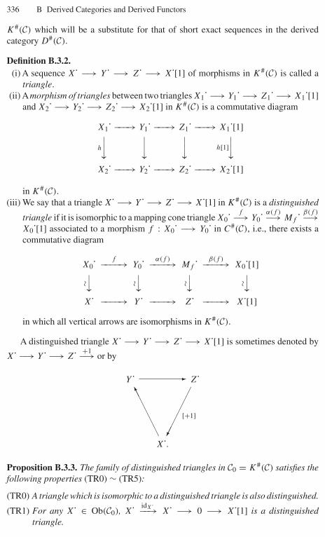
336 B Derived Categories and Derived Functors
K#(C) which will be a substitute for that of short exact sequences in the derivedcategory D#(C).
Definition B.3.2.(i) A sequence X˙ −→ Y˙ −→ Z˙ −→ X˙[1] of morphisms in K#(C) is called a
triangle.(ii) Amorphism of triangles between two triangles X1˙ −→ Y1˙ −→ Z1˙ −→ X1˙[1]
and X2˙ −→ Y2˙ −→ Z2˙ −→ X2˙[1] in K#(C) is a commutative diagram
X1˙ −−−→ Y1˙ −−−→ Z1˙ −−−→ X1˙[1]⏐⏐⏐h ⏐⏐⏐ ⏐⏐⏐ ⏐⏐⏐h[1]
X2˙ −−−→ Y2˙ −−−→ Z2˙ −−−→ X2˙[1]
in K#(C).(iii) We say that a triangle X˙ −→ Y˙ −→ Z˙ −→ X˙[1] in K#(C) is a distinguished
triangle if it is isomorphic to a mapping cone triangle X0˙ f−→ Y0˙ α(f )−→ Mf ˙ β(f )−→X0˙[1] associated to a morphism f : X0˙ −→ Y0˙ in C#(C), i.e., there exists acommutative diagram
X0˙ f−−−−→ Y0˙ α(f )−−−−→ Mf ˙ β(f )−−−−→ X0˙[1]�⏐⏐ �
⏐⏐ �⏐⏐ �
⏐⏐X˙ −−−−→ Y˙ −−−−→ Z˙ −−−−→ X˙[1]
in which all vertical arrows are isomorphisms in K#(C).
A distinguished triangle X˙ −→ Y˙ −→ Z˙ −→ X˙[1] is sometimes denoted by
X˙ −→ Y˙ −→ Z˙ +1−→ or by
Y˙ Z˙
X .
�
��
��
���
[+1]
��
��
���
Proposition B.3.3. The family of distinguished triangles in C0 = K#(C) satisfies thefollowing properties (TR0) ∼ (TR5):
(TR0) A triangle which is isomorphic to a distinguished triangle is also distinguished.
(TR1) For any X˙ ∈ Ob(C0), X˙ idX˙−−→ X˙ −→ 0 −→ X˙[1] is a distinguishedtriangle.
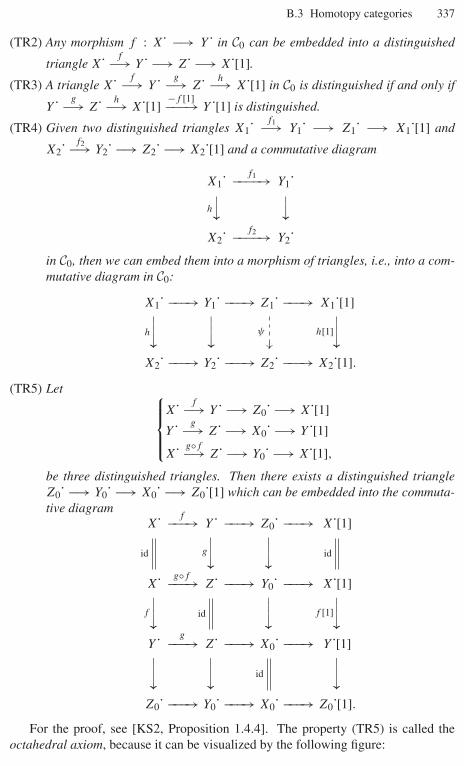
B.3 Homotopy categories 337
(TR2) Any morphism f : X˙ −→ Y˙ in C0 can be embedded into a distinguished
triangle X˙ f−→ Y˙ −→ Z˙ −→ X˙[1].(TR3) A triangle X˙ f−→ Y˙ g−→ Z˙ h−→ X˙[1] in C0 is distinguished if and only if
Y˙ g−→ Z˙ h−→ X˙[1] −f [1]−−−→ Y˙[1] is distinguished.
(TR4) Given two distinguished triangles X1˙ f1−→ Y1˙ −→ Z1˙ −→ X1˙[1] and
X2˙ f2−→ Y2˙ −→ Z2˙ −→ X2˙[1] and a commutative diagram
X1˙ f1−−−−→ Y1˙h
⏐⏐ ⏐⏐X2˙ f2−−−−→ Y2˙
in C0, then we can embed them into a morphism of triangles, i.e., into a com-mutative diagram in C0:
X1˙ −−−→ Y1˙ −−−→ Z1˙ −−−→ X1˙[1]⏐⏐⏐h ⏐⏐⏐ ψ
⏐⏐⏐h[1]
X2˙ −−−→ Y2˙ −−−→ Z2˙ −−−→ X2˙[1].(TR5) Let ⎧⎪⎪⎨⎪⎪⎩
X˙ f−→ Y˙ −→ Z0˙ −→ X˙[1]Y˙ g−→ Z˙ −→ X0˙ −→ Y˙[1]X˙ g◦f−→ Z˙ −→ Y0˙ −→ X˙[1],
be three distinguished triangles. Then there exists a distinguished triangleZ0˙ −→ Y0˙ −→ X0˙ −→ Z0˙[1] which can be embedded into the commuta-tive diagram
X˙ −−−→fY˙ −−−→ Z0˙ −−−→ X˙[1]
id
⏐⏐⏐g ⏐⏐⏐ id
X˙ −−−→g◦fZ˙ −−−→ Y0˙ −−−→ X˙[1]⏐⏐⏐f id
⏐⏐⏐ ⏐⏐⏐f [1]
Y˙ −−−→gZ˙ −−−→ X0˙ −−−→ Y˙[1]⏐⏐⏐ ⏐⏐⏐ id
⏐⏐⏐Z0˙ −−−→ Y0˙ −−−→ X0˙ −−−→ Z0˙[1].
For the proof, see [KS2, Proposition 1.4.4]. The property (TR5) is called theoctahedral axiom, because it can be visualized by the following figure:
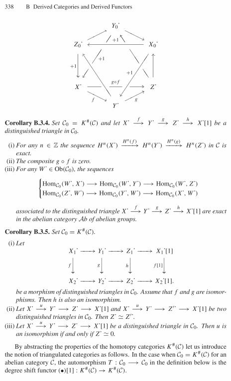
338 B Derived Categories and Derived Functors
Y0˙
Z0˙
X˙
Y˙
Z˙
X0˙+1
g◦f
+1
+1
+1
f g
���
��� ���
���
��
��
��� �
��
��
��
��
���
����
���
��
Corollary B.3.4. Set C0 = K#(C) and let X˙ f−→ Y˙ g−→ Z˙ h−→ X˙[1] be adistinguished triangle in C0.
(i) For any n ∈ Z the sequence Hn(X˙) Hn(f )−−−→ Hn(Y˙) Hn(g)−−−→ Hn(Z˙) in C isexact.
(ii) The composite g ◦ f is zero.(iii) For any W˙ ∈ Ob(C0), the sequences{
HomC0(W˙, X˙) −→ HomC0(W˙, Y˙) −→ HomC0(W˙, Z˙)HomC0(Z˙, W˙) −→ HomC0(Y˙, W˙) −→ HomC0(X˙, W˙)
associated to the distinguished triangle X˙ f−→ Y˙ g−→ Z˙ h−→ X˙[1] are exactin the abelian category Ab of abelian groups.
Corollary B.3.5. Set C0 = K#(C).
(i) LetX1˙ −−−→ Y1˙ −−−→ Z1˙ −−−→ X1˙[1]⏐⏐⏐f
⏐⏐⏐g ⏐⏐⏐h ⏐⏐⏐f [1]
X2˙ −−−→ Y2˙ −−−→ Z2˙ −−−→ X2˙[1].be a morphism of distinguished triangles in C0. Assume that f and g are isomor-phisms. Then h is also an isomorphism.
(ii) Let X˙ u−→ Y˙ −→ Z˙ −→ X˙[1] and X˙ u−→ Y˙ −→ Z′˙ −→ X˙[1] be twodistinguished triangles in C0. Then Z˙ � Z′ .
(iii) Let X˙ u−→ Y˙ −→ Z˙ −→ X˙[1] be a distinguished triangle in C0. Then u isan isomorphism if and only if Z˙ � 0.
By abstracting the properties of the homotopy categories K#(C) let us introducethe notion of triangulated categories as follows. In the case when C0 = K#(C) for anabelian category C, the automorphism T : C0 −→ C0 in the definition below is thedegree shift functor (•)[1] : K#(C) → K#(C).
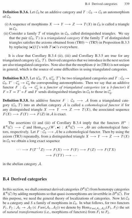
B.4 Derived categories 339
Definition B.3.6. Let C0 be an additive category and T : C0 → C0 an automorphismof C0.
(i) A sequence of morphisms X −→ Y −→ Z −→ T (X) in C0 is called a trianglein C0.
(ii) Consider a family T of triangles in C0, called distinguished triangles. We saythat the pair (C0, T ) is a triangulated category if the family T of distinguishedtriangles satisfies the axioms obtained from (TR0) ∼ (TR5) in Proposition B.3.3by replacing (•)[1]’s with T (•)’s everywhere.
It is clear that Corollary B.3.4 (ii), (iii) and Corollary B.3.5 are true for anytriangulated category (C0, T ). Derived categories that we introduce in the next sectionare also triangulated categories. Note also that the morphism ψ in (TR4) is not uniquein general, which is the source of some difficulties in using triangulated categories.
Definition B.3.7. Let (C0, T ), (C′0, T ′) be two triangulated categories and T : C0 →
C0, T ′ : C′0 → C′
0 the corresponding automorphisms. Then we say that an additivefunctor F : C0 → C′
0 is a functor of triangulated categories (or a ∂-functor) ifF ◦ T = T ′ ◦ F and F sends distinguished triangles in C0 to those in C′
0.
Definition B.3.8. An additive functor F : C0 −→ A from a triangulated cate-gory (C0, T ) into an abelian category A is called a cohomological functor if forany distinguished triangle X −→ Y −→ Z −→ T (X), the associated sequenceF(X) −→ F(Y ) −→ F(Z) in A is exact.
The assertions (i) and (iii) of Corollary B.3.4 imply that the functors Hn :K#(C) −→ C and HomK#(C)(W˙, •) : K#(C) −→ Ab are cohomological func-tors, respectively. Let F : C0 −→ A be a cohomological functor. Then by using theaxiom (TR3) repeatedly, from a distinguished triangle X −→ Y −→ Z −→ T (X)
in C0 we obtain a long exact sequence
· · · −→ F(T −1Z) −→ F(X) −→ F(Y ) −→ F(Z) −→ F(T X)
−→ F(T Y ) −→ · · ·in the abelian category A.
B.4 Derived categories
In this section, we shall construct derived categories D#(C) from homotopy categoriesK#(C) by adding morphisms so that quasi-isomorphisms are invertible in D#(C). Forthis purpose, we need the general theory of localizations of categories. Now let C0be a category and S a family of morphisms in C0. In what follows, for two functorsF1, F2 : A1 → A2 (∈ Fun(A1, A2)) we denote by HomFun(A1,A2)(F1, F2) the setof natural transformations (i.e., morphisms of functors) from F1 to F2.
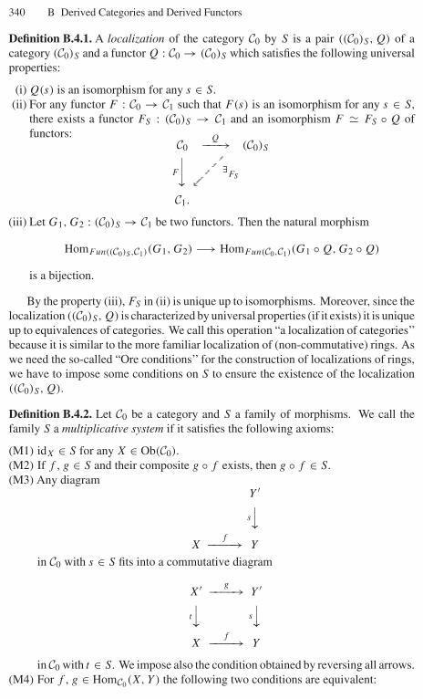
340 B Derived Categories and Derived Functors
Definition B.4.1. A localization of the category C0 by S is a pair ((C0)S, Q) of acategory (C0)S and a functor Q : C0 → (C0)S which satisfies the following universalproperties:
(i) Q(s) is an isomorphism for any s ∈ S.(ii) For any functor F : C0 → C1 such that F(s) is an isomorphism for any s ∈ S,
there exists a functor FS : (C0)S → C1 and an isomorphism F � FS ◦ Q offunctors:
C0 −−−→Q(C0)S⏐⏐⏐F ∃
FS
C1.
(iii) Let G1, G2 : (C0)S → C1 be two functors. Then the natural morphism
HomFun((C0)S ,C1)(G1, G2) −→ HomFun(C0,C1)(G1 ◦ Q, G2 ◦ Q)
is a bijection.
By the property (iii), FS in (ii) is unique up to isomorphisms. Moreover, since thelocalization ((C0)S, Q) is characterized by universal properties (if it exists) it is uniqueup to equivalences of categories. We call this operation “a localization of categories’’because it is similar to the more familiar localization of (non-commutative) rings. Aswe need the so-called “Ore conditions’’ for the construction of localizations of rings,we have to impose some conditions on S to ensure the existence of the localization((C0)S, Q).
Definition B.4.2. Let C0 be a category and S a family of morphisms. We call thefamily S a multiplicative system if it satisfies the following axioms:
(M1) idX ∈ S for any X ∈ Ob(C0).(M2) If f , g ∈ S and their composite g ◦ f exists, then g ◦ f ∈ S.(M3) Any diagram
Y ′
s
⏐⏐X
f−−−−→ Y
in C0 with s ∈ S fits into a commutative diagram
X′ g−−−−→ Y ′
t
⏐⏐ s
⏐⏐X
f−−−−→ Y
in C0 with t ∈ S. We impose also the condition obtained by reversing all arrows.(M4) For f , g ∈ HomC0(X, Y ) the following two conditions are equivalent:
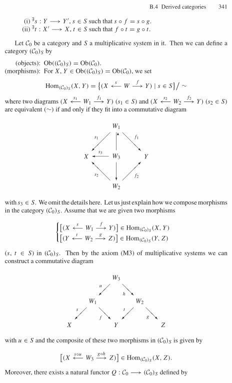
B.4 Derived categories 341
(i) ∃s : Y −→ Y ′, s ∈ S such that s ◦ f = s ◦ g.(ii) ∃t : X′ −→ X, t ∈ S such that f ◦ t = g ◦ t .
Let C0 be a category and S a multiplicative system in it. Then we can define acategory (C0)S by
(objects): Ob((C0)S) = Ob(C0).(morphisms): For X, Y ∈ Ob((C0)S) = Ob(C0), we set
Hom(C0)S(X, Y ) = {
(Xs←− W
f−→ Y ) | s ∈ S}/ ∼
where two diagrams (Xs1←− W1
f1−→ Y ) (s1 ∈ S) and (Xs2←− W2
f2−→ Y ) (s2 ∈ S)
are equivalent (∼) if and only if they fit into a commutative diagram
W1
X W3 Y
W2
��
��
s1 ��
��
f1
�
�s3
�
��
��s2 �
���f2
with s3 ∈ S. We omit the details here. Let us just explain how we compose morphismsin the category (C0)S . Assume that we are given two morphisms{[
(Xs←− W1
f−→ Y )] ∈ Hom(C0)S
(X, Y )[(Y
t←− W2g−→ Z)
] ∈ Hom(C0)S(Y, Z)
(s, t ∈ S) in (C0)S . Then by the axiom (M3) of multiplicative systems we canconstruct a commutative diagram
W3
W1 W2
X Y Z
���u �
��h
���s �
��f�
��t �
��g
with u ∈ S and the composite of these two morphisms in (C0)S is given by[(X
s◦u←− W3g◦h−→ Z)
] ∈ Hom(C0)S(X, Z).
Moreover, there exists a natural functor Q : C0 −→ (C0)S defined by
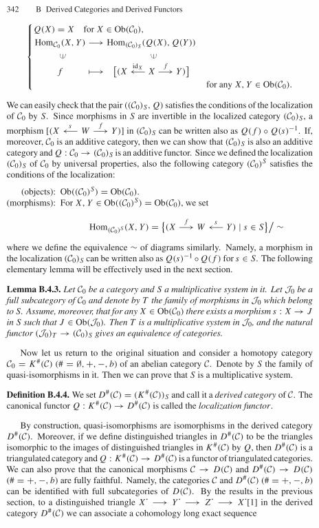
342 B Derived Categories and Derived Functors⎧⎪⎪⎪⎪⎪⎪⎨⎪⎪⎪⎪⎪⎪⎩
Q(X) = X for X ∈ Ob(C0),
HomC0(X, Y ) −→ Hom(C0)S(Q(X), Q(Y ))
�� ��f �−→ [
(XidX←− X
f−→ Y )]
for any X, Y ∈ Ob(C0).
We can easily check that the pair ((C0)S, Q) satisfies the conditions of the localizationof C0 by S. Since morphisms in S are invertible in the localized category (C0)S , a
morphism [(X s←− Wf−→ Y )] in (C0)S can be written also as Q(f ) ◦ Q(s)−1. If,
moreover, C0 is an additive category, then we can show that (C0)S is also an additivecategory and Q : C0 → (C0)S is an additive functor. Since we defined the localization(C0)S of C0 by universal properties, also the following category (C0)S satisfies theconditions of the localization:
(objects): Ob((C0)S) = Ob(C0).(morphisms): For X, Y ∈ Ob((C0)S) = Ob(C0), we set
Hom(C0)S (X, Y ) = {(X
f−→ Ws←− Y ) | s ∈ S
}/ ∼where we define the equivalence ∼ of diagrams similarly. Namely, a morphism inthe localization (C0)S can be written also as Q(s)−1 ◦Q(f ) for s ∈ S. The followingelementary lemma will be effectively used in the next section.
Lemma B.4.3. Let C0 be a category and S a multiplicative system in it. Let J0 be afull subcategory of C0 and denote by T the family of morphisms in J0 which belongto S. Assume, moreover, that for any X ∈ Ob(C0) there exists a morphism s : X → J
in S such that J ∈ Ob(J0). Then T is a multiplicative system in J0, and the naturalfunctor (J0)T → (C0)S gives an equivalence of categories.
Now let us return to the original situation and consider a homotopy categoryC0 = K#(C) (# = ∅, +, −, b) of an abelian category C. Denote by S the family ofquasi-isomorphisms in it. Then we can prove that S is a multiplicative system.
Definition B.4.4. We set D#(C) = (K#(C))S and call it a derived category of C. Thecanonical functor Q : K#(C) → D#(C) is called the localization functor.
By construction, quasi-isomorphisms are isomorphisms in the derived categoryD#(C). Moreover, if we define distinguished triangles in D#(C) to be the trianglesisomorphic to the images of distinguished triangles in K#(C) by Q, then D#(C) is atriangulated category and Q : K#(C) → D#(C) is a functor of triangulated categories.We can also prove that the canonical morphisms C → D(C) and D#(C) → D(C)
(# = +, −, b) are fully faithful. Namely, the categories C and D#(C) (# = +, −, b)can be identified with full subcategories of D(C). By the results in the previoussection, to a distinguished triangle X˙ −→ Y˙ −→ Z˙ −→ X˙[1] in the derivedcategory D#(C) we can associate a cohomology long exact sequence
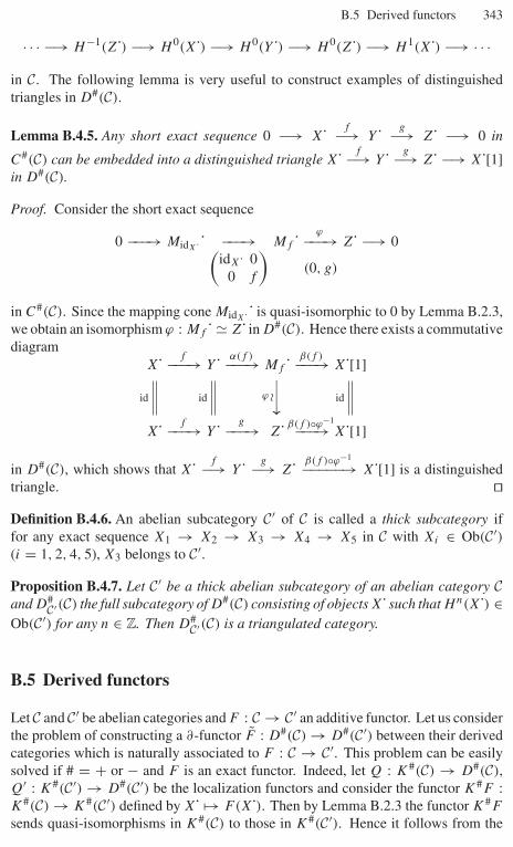
B.5 Derived functors 343
· · · −→ H−1(Z˙) −→ H 0(X˙) −→ H 0(Y˙) −→ H 0(Z˙) −→ H 1(X˙) −→ · · ·in C. The following lemma is very useful to construct examples of distinguishedtriangles in D#(C).
Lemma B.4.5. Any short exact sequence 0 −→ X˙ f−→ Y˙ g−→ Z˙ −→ 0 in
C#(C) can be embedded into a distinguished triangle X˙ f−→ Y˙ g−→ Z˙ −→ X˙[1]in D#(C).
Proof. Consider the short exact sequence
0 −−−→ MidX˙ ˙ −−−→ Mf ˙ −−−→ϕZ˙ −→ 0(
idX˙ 00 f
)(0, g)
in C#(C). Since the mapping cone MidX˙ ˙ is quasi-isomorphic to 0 by Lemma B.2.3,we obtain an isomorphism ϕ : Mf ˙ � Z˙ in D#(C). Hence there exists a commutativediagram
X˙ −−−→fY˙ −−−→α(f )
Mf ˙ −−−→β(f )X˙[1]
id id
⏐⏐⏐ϕ � id
X˙ −−−→fY˙ −−−→g
Z˙ −−−→β(f )◦ϕ−1
X˙[1]
in D#(C), which shows that X˙ f−→ Y˙ g−→ Z˙ β(f )◦ϕ−1
−−−−−→ X˙[1] is a distinguishedtriangle. ��Definition B.4.6. An abelian subcategory C′ of C is called a thick subcategory iffor any exact sequence X1 → X2 → X3 → X4 → X5 in C with Xi ∈ Ob(C′)(i = 1, 2, 4, 5), X3 belongs to C′.
Proposition B.4.7. Let C′ be a thick abelian subcategory of an abelian category Cand D#
C′(C) the full subcategory of D#(C) consisting of objects X˙ such that Hn(X˙) ∈Ob(C′) for any n ∈ Z. Then D#
C′(C) is a triangulated category.
B.5 Derived functors
Let C and C′ be abelian categories and F : C → C′ an additive functor. Let us considerthe problem of constructing a ∂-functor F : D#(C) → D#(C′) between their derivedcategories which is naturally associated to F : C → C′. This problem can be easilysolved if # = + or − and F is an exact functor. Indeed, let Q : K#(C) → D#(C),Q′ : K#(C′) → D#(C′) be the localization functors and consider the functor K#F :K#(C) → K#(C′) defined by X˙ �→ F(X˙). Then by Lemma B.2.3 the functor K#F
sends quasi-isomorphisms in K#(C) to those in K#(C′). Hence it follows from the
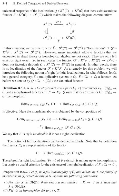
344 B Derived Categories and Derived Functors
universal properties of the localization Q : K#(C) → D#(C) that there exists a uniquefunctor F : D#(C) → D#(C′) which makes the following diagram commutative:
K#(C)K#F−−−−→ K#(C′)
Q
⏐⏐ ⏐⏐Q′
D#(C) −−−−→F
D#(C′).
In this situation, we call the functor F : D#(C) → D#(C′) a “localization’’ of Q′ ◦K#F : K#(C) → D#(C′). However, many important additive functors that weencounter in sheaf theory or homological algebra are not exact. They are only leftexact or right exact. So in such cases the functor Q′ ◦ K#F : K#(C) → D#(C′)does not factorize through Q : K#(C) → D#(C) in general. In other words, thereis no localization of the functor Q′ ◦ K#F . As a remedy for this problem we willintroduce the following notion of right (or left) localizations. In what follows, let C0be a general category, S a multiplicative system in C0, F : C0 → C1 a functor. Asbefore we denote by Q : C0 → (C0)S the canonical functor.
Definition B.5.1. A right localization of F is a pair (FS, τ ) of a functor FS : (C0)S →C1 and a morphism of functors τ : F → FS ◦Q such that for any functor G : (C0)S →C1 the morphism
HomFun((C0)S ,C1)(FS, G) −→ HomFun(C0,C1)(F, G ◦ Q)
is bijective. Here the morphism above is obtained by the composition of
HomFun((C0)S ,C1)(FS, G) −→ HomFun(C0,C1)(FS ◦ Q, G ◦ Q)
τ−→ HomFun(C0,C1)(F, G ◦ Q).
We say that F is right localizable if it has a right localization.
The notion of left localizations can be defined similarly. Note that by definitionthe functor FS is a representative of the functor
G −→ HomFun(C0,C1)(F, G ◦ Q).
Therefore, if a right localization (FS, τ ) of F exists, it is unique up to isomorphisms.Let us give a useful criterion for the existence of the right localization of F : C0 → C1.
Proposition B.5.2. Let J0 be a full subcategory of C0 and denote by T the family ofmorphisms in J0 which belong to S. Assume the following conditions:
(i) For any X ∈ Ob(C0) there exists a morphism s : X → J in S such thatJ ∈ Ob(J0).
(ii) F(t) is an isomorphism for any t ∈ T .
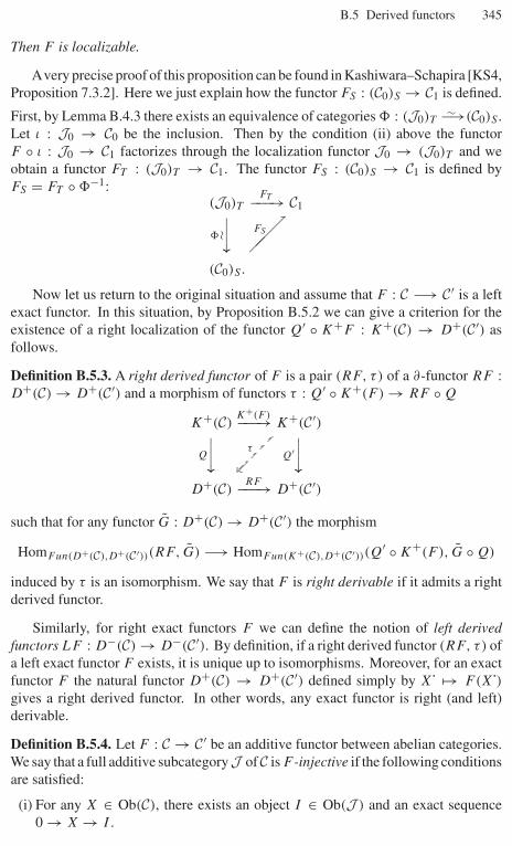
B.5 Derived functors 345
Then F is localizable.
Avery precise proof of this proposition can be found in Kashiwara–Schapira [KS4,Proposition 7.3.2]. Here we just explain how the functor FS : (C0)S → C1 is defined.
First, by Lemma B.4.3 there exists an equivalence of categories � : (J0)T −→∼ (C0)S .Let ι : J0 → C0 be the inclusion. Then by the condition (ii) above the functorF ◦ ι : J0 → C1 factorizes through the localization functor J0 → (J0)T and weobtain a functor FT : (J0)T → C1. The functor FS : (C0)S → C1 is defined byFS = FT ◦ �−1:
(J0)T −−−→FT C1⏐⏐⏐�� ���FS
(C0)S.
Now let us return to the original situation and assume that F : C −→ C′ is a leftexact functor. In this situation, by Proposition B.5.2 we can give a criterion for theexistence of a right localization of the functor Q′ ◦ K+F : K+(C) → D+(C′) asfollows.
Definition B.5.3. A right derived functor of F is a pair (RF, τ) of a ∂-functor RF :D+(C) → D+(C′) and a morphism of functors τ : Q′ ◦ K+(F ) → RF ◦ Q
K+(C) −−−→K+(F )K+(C′)⏐⏐⏐Q
τ
⏐⏐⏐Q′
D+(C) −−−→RFD+(C′)
such that for any functor G : D+(C) → D+(C′) the morphism
HomFun(D+(C),D+(C′))(RF, G) −→ HomFun(K+(C),D+(C′))(Q′ ◦ K+(F ), G ◦ Q)
induced by τ is an isomorphism. We say that F is right derivable if it admits a rightderived functor.
Similarly, for right exact functors F we can define the notion of left derivedfunctors LF : D−(C) → D−(C′). By definition, if a right derived functor (RF, τ) ofa left exact functor F exists, it is unique up to isomorphisms. Moreover, for an exactfunctor F the natural functor D+(C) → D+(C′) defined simply by X˙ �→ F(X˙)gives a right derived functor. In other words, any exact functor is right (and left)derivable.
Definition B.5.4. Let F : C → C′ be an additive functor between abelian categories.We say that a full additive subcategory J of C is F -injective if the following conditionsare satisfied:
(i) For any X ∈ Ob(C), there exists an object I ∈ Ob(J ) and an exact sequence0 → X → I .
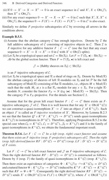
346 B Derived Categories and Derived Functors
(ii) If 0 → X′ → X → X′′ → 0 is an exact sequence in C and X′, X ∈ Ob(J ),then X′′ ∈ Ob(J ).
(iii) For any exact sequence 0 → X′ → X → X′′ → 0 in C such that X′, X, X′′ ∈Ob(J ), the sequence 0 → F(X′) → F(X) → F(X′′) → 0 in C′ is also exact.
Similarly we define F -projective subcategories of C by reversing all arrows in theconditions above.
Example B.5.5.(i) Assume that the abelian category C has enough injectives. Denote by I the
full additive subcategory of C consisting of injective objects in C. Then I isF -injective for any additive functor F : C → C′ (use the fact that any exactsequence 0 → X′ → X → X′′ → 0 in C with X′ ∈ Ob(I) splits).
(ii) Let T0 be a topological space and set C = Sh(T0). Let F = �(T0, •) : Sh(T0) →Ab be the global section functor. Then F = �(T0, •) is left exact and
J = {flabby sheaves on T0} ⊂ Sh(T0)
is an F -injective subcategory of C.(iii) Let T0 be a topological space and R a sheaf of rings on T0. Denote by Mod(R)
the abelian category of sheaves of left R-modules on T0 and let P be the fullsubcategory of Mod(R) consisting of flat R-modules, i.e., objects M ∈ Mod(R)
such that the stalk Mx at x is a flat Rx-module for any x ∈ T0. For a right R-module N , consider the functor FN = N ⊗R (•) : Mod(R) → Sh(T0). Thenthe category P is FN -projective. For the details see Section C.1.
Assume that for the given left exact functor F : C → C′ there exists an F -injective subcategory J of C. Then it is well known that for any X˙ ∈ Ob(K+(C))
we can construct a quasi-isomorphism X˙ → J˙ into an object J˙ of K+(J ). Suchan object J˙ is called an F -injective resolution of X . Moreover, by Lemma B.2.3we see that the functor Q′ ◦ K+F : K+(J ) → D+(C′) sends quasi-isomorphismsin K+(J ) to isomorphisms in D+(C′). Therefore, applying Proposition B.5.2 to thespecial case when C0 = K+(C), C1 = D+(C′), J0 = K+(J ) and S is the family ofquasi-isomorphisms in K+(C), we obtain the fundamental important result.
Theorem B.5.6. Let F : C → C′ be a left (resp. right) exact functor and assumethat there exists an F -injective (resp. F -projective) subcategory of C. Then the right(resp. left) derived functor RF : D+(C) → D+(C′) (resp. LF : D−(C) → D−(C′))of F exists.
Let F : C → C′ be a left exact functor and J an F -injective subcategory of C.Then the right derived functor RF : D+(C) → D+(C′) is constructed as follows.Denote by S (resp. T ) the family of quasi-isomorphisms in K+(C) (resp. K+(J )).
Then there exist an equivalence of categories � : K+(J )T −→∼ K+(C)S = D+(C)
and a natural functor & : K+(J )T → D+(C′) induced by K+F : K+(C) → K+(C′)such that RF = & ◦ �−1. Consequently the right derived functor RF : D+(C) →D+(C′) sends X˙ ∈ Ob(D+(C)) to F(J˙) ∈ Ob(D+(C′)), where J˙ ∈ Ob(K+(J ))

B.6 Bifunctors in derived categories 347
is an F -injective resolution of X . If C has enough injectives and denote by I thefull subcategory of C consisting of injective objects in C, then we have, moreover,an equivalence of categories K+(I) � D+(C). This follows from the basic factthat quasi-isomorphisms in K+(I) are homotopy equivalences. Using this explicitdescription of derived functors, we obtain the following useful composition rule.
Proposition B.5.7. Let C, C′, C′′ be abelian categories and F : C → C′, G : C′ → C′′left exact functors. Assume that C (resp. C′) has an F -injective (resp. G-injective)
subcategory J (resp. J ′) and F(X) ∈ Ob(J ′) for any X ∈ Ob(J ). Then J is(G ◦ F)-injective and
R(G ◦ F) = RG ◦ RF : D+(C) −→ D+(C′′).
Definition B.5.8. Assume that a left exact functor F : C → C′ is right derivable.Then for each n ∈ Z we set
RnF = Hn ◦ RF : D+(C) → C′.
Since RF : D+(C) → D+(C′) sends distinguished triangles to distinguishedtriangles, the functors RnF : D+(C) → C′ defined above are cohomological functors.Now let us identify C with the full subcategory of D+(C) consisting of complexesconcentrated in degree 0. Then we find that for X ∈ Ob(C), RnF(X) ∈ Ob(C′)coincides with the nth derived functor of F in the classical literature.
B.6 Bifunctors in derived categories
In this section we introduce some important bifunctors in derived categories whichwill be frequently used throughout this book. First, let us explain the bifunctorRHom(•, •). Let C be an abelian category. For two complexes X , Y˙ ∈ Ob(C(C))
in C define a new complex Hom ˙(X˙, Y˙) ∈ Ob(C(Ab)) by⎧⎪⎪⎪⎪⎪⎪⎪⎨⎪⎪⎪⎪⎪⎪⎪⎩
Homn(X˙, Y˙) =∏
j−i=n
HomC(Xi, Y j )
dn = dnHom ˙(X˙,Y ˙) :
∏j−i=n
HomC(Xi, Y j ) −→∏
j−i=n+1
HomC(Xi, Y j )
�� ��{fij } �−→ {
gij = (−1)n+1fi+1,j ◦ diX˙ + d
j−1Y ˙ ◦ fi,j−1
}.
This is the simple complex associated to the double complex Hom(X˙, Y˙), whichsatisfies the conditions⎧⎪⎨⎪⎩
Ker dn � HomC(C)(X˙, Y˙[n])Im dn−1 � Ht(X˙, Y˙[n])Hn[Hom ˙(X˙, Y˙)] � HomK(C)(X˙, Y˙[n]).
for any n ∈ Z. We thus defined a bifunctor
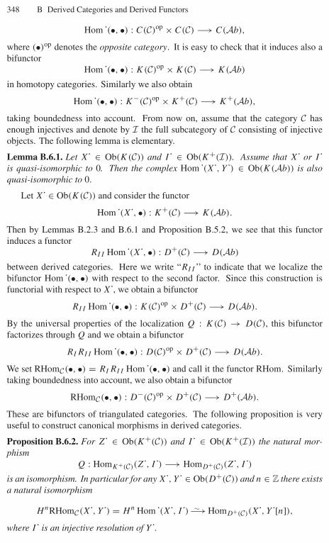
348 B Derived Categories and Derived Functors
Hom ˙(•, •) : C(C)op × C(C) −→ C(Ab),
where (•)op denotes the opposite category. It is easy to check that it induces also abifunctor
Hom ˙(•, •) : K(C)op × K(C) −→ K(Ab)
in homotopy categories. Similarly we also obtain
Hom ˙(•, •) : K−(C)op × K+(C) −→ K+(Ab),
taking boundedness into account. From now on, assume that the category C hasenough injectives and denote by I the full subcategory of C consisting of injectiveobjects. The following lemma is elementary.
Lemma B.6.1. Let X˙ ∈ Ob(K(C)) and I˙ ∈ Ob(K+(I)). Assume that X˙ or I˙is quasi-isomorphic to 0. Then the complex Hom ˙(X˙, Y˙) ∈ Ob(K(Ab)) is alsoquasi-isomorphic to 0.
Let X˙ ∈ Ob(K(C)) and consider the functor
Hom ˙(X˙, •) : K+(C) −→ K(Ab).
Then by Lemmas B.2.3 and B.6.1 and Proposition B.5.2, we see that this functorinduces a functor
RII Hom ˙(X˙, •) : D+(C) −→ D(Ab)
between derived categories. Here we write “RII ’’ to indicate that we localize thebifunctor Hom ˙(•, •) with respect to the second factor. Since this construction isfunctorial with respect to X , we obtain a bifunctor
RII Hom ˙(•, •) : K(C)op × D+(C) −→ D(Ab).
By the universal properties of the localization Q : K(C) → D(C), this bifunctorfactorizes through Q and we obtain a bifunctor
RI RII Hom ˙(•, •) : D(C)op × D+(C) −→ D(Ab).
We set RHomC(•, •) = RI RII Hom ˙(•, •) and call it the functor RHom. Similarlytaking boundedness into account, we also obtain a bifunctor
RHomC(•, •) : D−(C)op × D+(C) −→ D+(Ab).
These are bifunctors of triangulated categories. The following proposition is veryuseful to construct canonical morphisms in derived categories.
Proposition B.6.2. For Z˙ ∈ Ob(K+(C)) and I˙ ∈ Ob(K+(I)) the natural mor-phism
Q : HomK+(C)(Z˙, I˙) −→ HomD+(C)(Z˙, I˙)is an isomorphism. In particular for any X˙, Y˙ ∈ Ob(D+(C)) and n ∈ Z there existsa natural isomorphism
HnRHomC(X˙, Y˙) = Hn Hom ˙(X˙, I˙) −→∼ HomD+(C)(X˙, Y˙[n]),where I˙ is an injective resolution of Y .
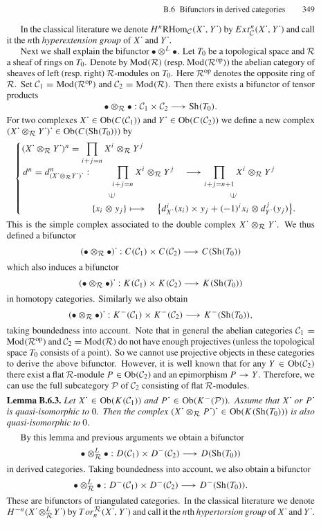
B.6 Bifunctors in derived categories 349
In the classical literature we denote HnRHomC(X˙, Y˙) by ExtnC(X˙, Y˙) and call
it the nth hyperextension group of X˙ and Y .Next we shall explain the bifunctor • ⊗L •. Let T0 be a topological space and R
a sheaf of rings on T0. Denote by Mod(R) (resp. Mod(Rop)) the abelian category ofsheaves of left (resp. right) R-modules on T0. Here Rop denotes the opposite ring ofR. Set C1 = Mod(Rop) and C2 = Mod(R). Then there exists a bifunctor of tensorproducts
• ⊗R • : C1 × C2 −→ Sh(T0).
For two complexes X˙ ∈ Ob(C(C1)) and Y˙ ∈ Ob(C(C2)) we define a new complex(X˙ ⊗R Y˙)˙ ∈ Ob(C(Sh(T0))) by⎧⎪⎪⎪⎪⎪⎪⎪⎨⎪⎪⎪⎪⎪⎪⎪⎩
(X˙ ⊗R Y˙)n =∏
i+j=n
Xi ⊗R Y j
dn = dn(X˙⊗RY ˙)˙ :
∏i+j=n
Xi ⊗R Y j −→∏
i+j=n+1
Xi ⊗R Y j
�� ��{xi ⊗ yj } �−→ {
diX˙(xi) × yj + (−1)ixi ⊗ d
jY ˙(yj )
}.
This is the simple complex associated to the double complex X˙ ⊗R Y . We thusdefined a bifunctor
(• ⊗R •)˙ : C(C1) × C(C2) −→ C(Sh(T0))
which also induces a bifunctor
(• ⊗R •)˙ : K(C1) × K(C2) −→ K(Sh(T0))
in homotopy categories. Similarly we also obtain
(• ⊗R •)˙ : K−(C1) × K−(C2) −→ K−(Sh(T0)),
taking boundedness into account. Note that in general the abelian categories C1 =Mod(Rop) and C2 = Mod(R) do not have enough projectives (unless the topologicalspace T0 consists of a point). So we cannot use projective objects in these categoriesto derive the above bifunctor. However, it is well known that for any Y ∈ Ob(C2)
there exist a flat R-module P ∈ Ob(C2) and an epimorphism P → Y . Therefore, wecan use the full subcategory P of C2 consisting of flat R-modules.
Lemma B.6.3. Let X˙ ∈ Ob(K(C1)) and P ˙ ∈ Ob(K−(P)). Assume that X˙ or P ˙is quasi-isomorphic to 0. Then the complex (X˙ ⊗R P ˙)˙ ∈ Ob(K(Sh(T0))) is alsoquasi-isomorphic to 0.
By this lemma and previous arguments we obtain a bifunctor
• ⊗LR • : D(C1) × D−(C2) −→ D(Sh(T0))
in derived categories. Taking boundedness into account, we also obtain a bifunctor
• ⊗LR • : D−(C1) × D−(C2) −→ D−(Sh(T0)).
These are bifunctors of triangulated categories. In the classical literature we denoteH−n(X˙⊗L
R Y˙) by T orRn (X˙, Y˙) and call it the nth hypertorsion group of X˙ and Y .

C
Sheaves and Functors in Derived Categories
In this appendix, assuming only few prerequisites for sheaf theory, we introducebasic operations of sheaves in derived categories and their main properties with-out proofs. For the details we refer to Hartshorne [Ha1], Iversen [Iv], Kashiwara–Schapira [KS2], [KS4]. We also give a proof of Kashiwara’s non-characteristicdeformation lemma.
C.1 Sheaves and functors
In this section we quickly recall basic operations in sheaf theory. For a topologicalspace X we denote by Sh(X) the abelian category of sheaves on X. The abelian groupof sections of F ∈ Sh(X) on an open subset U ⊂ X is denoted by F(U) or �(U, F ),and the subgroup of �(U, F ) consisting of sections with compact supports is denotedby �c(U, F ). We thus obtain left exact functors �(U, •), �c(U, •) : Sh(X) → Ab
for each open subset U ⊂ X, where Ab denotes the abelian category of abeliangroups. If R is a sheaf of rings on X, we denote by Mod(R) (resp. Mod(Rop)) theabelian category of sheaves of left (resp. right) R-modules on X. Here Rop denotesthe opposite ring of R. For example, in the case where R is the constant sheafZX with germs Z the category Mod(R) is Sh(X). For F, G ∈ Sh(X) (resp. M, N
∈ Mod(R)) we denote by Hom(F, G) (resp. HomR(M, N)) the abelian group ofsheaf homomorphisms (resp. sheaf homomorphisms commuting with the actions ofR) on X from F to G (resp. from M to N ). We thus obtain left exact bifunctors{
Hom(•, •) : Sh(X)op × Sh(X) −→ Ab,
HomR(•, •) : Mod(R)op × Mod(R) −→ Ab.
For a subset Z ⊂ X, we denote by iZ : Z → X the inclusion map.
Definition C.1.1. Let f : X → Y be a morphism of topological spaces, F ∈ Sh(X)
and G ∈ Sh(Y ).

352 C Sheaves and Functors in Derived Categories
(i) The direct image f∗F ∈ Sh(Y ) of F by f is defined by f∗F(V ) = F(f −1(V ))
for each open subset V ⊂ Y . This gives a left exact functor f∗ : Sh(X) → Sh(Y ).If Y is the space pt consisting of one point, the functor f∗ is the global sectionfunctor �(X, •) : Sh(X) → Ab.
(ii) The proper direct image f!F ∈ Sh(Y ) of F by f is defined by f!F(V ) = {s ∈F(f −1(V ))|f |supp s : supp s → V is proper} for each open subset V ⊂ Y .This gives a left exact functor f! : Sh(X) → Sh(Y ). If Y is pt, the functor f! isthe global section functor with compact supports �c(X, •) : Sh(X) → Ab.
(iii) The inverse image f −1G ∈ Sh(X) of G by f is the sheaf associated to thepresheaf (f −1G)′ defined by (f −1G)′(U) = lim−→ G(V ) for each open subsetU ⊂ X, where V ranges through the family of open subsets of Y containingf (U). Since we have an isomorphism (f −1G)x � Gf (x) for any x ∈ X, weobtain an exact functor f −1 : Sh(Y ) → Sh(X).
When we treat proper direct images f! in this book, all topological spaces areassumed to be locally compact and Hausdorff. For two morphisms f : X → Y ,g : Y → Z of topological spaces, we have obvious relations g∗ ◦ f∗ = (g ◦ f )∗,g! ◦f! = (g◦f )! and f −1 ◦g−1 = (g◦f )−1. For F ∈ Sh(X) and a subset Z ⊂ X theinverse image i−1
Z F ∈ Sh(Z) of F by the inclusion map iZ : Z → X is sometimesdenoted by F |Z . If Z is a locally closed subset of X (i.e., a subset of X which iswritten as an intersection of an open subset and a closed subset), then it is well knownthat the functor (iZ)! : Sh(Z) → Sh(X) is exact.
Proposition C.1.2. Let
X′ f ′−−−−→ Y ′
g′⏐⏐ g
⏐⏐X
f−−−−→ Y
be a cartesian square of topological spaces, i.e., X′ is homeomorphic to the fiberproduct X×Y Y ′. Then there exists an isomorphism of functors g−1 ◦f! � f ′
! ◦g′−1 :Sh(X) → Sh(Y ′).
Definition C.1.3. Let X be a topological space, Z ⊂ X a locally closed subset andF ∈ Sh(X).
(i) Set FZ = (iZ)!(iZ)−1F ∈ Sh(X). Since we have (FZ)x � Fx (resp. (FZ)x � 0)for any x ∈ Z (resp. x ∈ X \ Z), we obtain an exact functor (•)Z : Sh(X) →Sh(X).
(ii) Take an open subset W of X containing Z as a closed subset of W . Since theabelian group Ker[F(W) → F(W \Z)] does not depend on the choice of W , wedenote it by �Z(X, F ). This gives a left exact functor �Z(X, •) : Sh(X) → Ab.
(iii) The subsheaf �Z(F ) of F is defined by �Z(F )(U) = �Z∩U (U, F |U ) for eachopen subset U ⊂ X. This gives a left exact functor �Z(•) : Sh(X) → Sh(X). Byconstruction we have an isomorphism of functors �(X, •) ◦ �Z(•) = �Z(X, •).
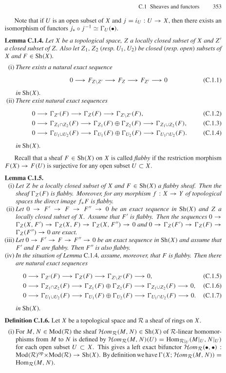
C.1 Sheaves and functors 353
Note that if U is an open subset of X and j = iU : U → X, then there exists anisomorphism of functors j∗ ◦ j−1 � �U (•).
Lemma C.1.4. Let X be a topological space, Z a locally closed subset of X and Z′a closed subset of Z. Also let Z1, Z2 (resp. U1, U2) be closed (resp. open) subsets ofX and F ∈ Sh(X).
(i) There exists a natural exact sequence
0 −→ FZ\Z′ −→ FZ −→ FZ′ −→ 0 (C.1.1)
in Sh(X).(ii) There exist natural exact sequences
0 −→ �Z′(F ) −→ �Z(F ) −→ �Z\Z′(F ), (C.1.2)
0 −→ �Z1∩Z2(F ) −→ �Z1(F ) ⊕ �Z2(F ) −→ �Z1∪Z2(F ), (C.1.3)
0 −→ �U1∪U2(F ) −→ �U1(F ) ⊕ �U2(F ) −→ �U1∩U2(F ). (C.1.4)
in Sh(X).
Recall that a sheaf F ∈ Sh(X) on X is called flabby if the restriction morphismF(X) → F(U) is surjective for any open subset U ⊂ X.
Lemma C.1.5.(i) Let Z be a locally closed subset of X and F ∈ Sh(X) a flabby sheaf. Then the
sheaf �Z(F ) is flabby. Moreover, for any morphism f : X → Y of topologicalspaces the direct image f∗F is flabby.
(ii) Let 0 → F ′ → F → F ′′ → 0 be an exact sequence in Sh(X) and Z alocally closed subset of X. Assume that F ′ is flabby. Then the sequences 0 →�Z(X, F ′) → �Z(X, F ) → �Z(X, F ′′) → 0 and 0 → �Z(F ′) → �Z(F ) →�Z(F ′′) → 0 are exact.
(iii) Let 0 → F ′ → F → F ′′ → 0 be an exact sequence in Sh(X) and assume thatF ′ and F are flabby. Then F ′′ is also flabby.
(iv) In the situation of Lemma C.1.4, assume, moreover, that F is flabby. Then thereare natural exact sequences
0 −→ �Z′(F ) −→ �Z(F ) −→ �Z\Z′(F ) −→ 0, (C.1.5)
0 −→ �Z1∩Z2(F ) −→ �Z1(F ) ⊕ �Z2(F ) −→ �Z1∪Z2(F ) −→ 0, (C.1.6)
0 −→ �U1∪U2(F ) −→ �U1(F ) ⊕ �U2(F ) −→ �U1∩U2(F ) −→ 0. (C.1.7)
in Sh(X).
Definition C.1.6. Let X be a topological space and R a sheaf of rings on X.
(i) For M, N ∈ Mod(R) the sheaf HomR(M, N) ∈ Sh(X) of R-linear homomor-phisms from M to N is defined by HomR(M, N)(U) = HomR|U (M|U , N |U )
for each open subset U ⊂ X. This gives a left exact bifunctor HomR(•, •) :Mod(R)op×Mod(R) → Sh(X). By definition we have �(X; HomR(M, N)) =HomR(M, N).
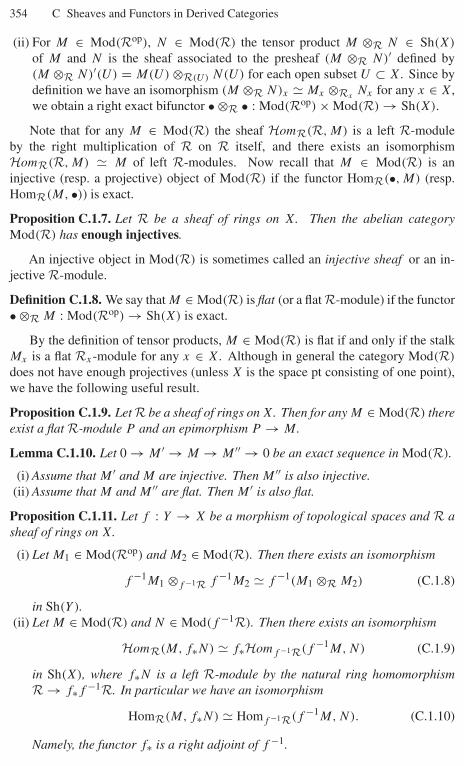
354 C Sheaves and Functors in Derived Categories
(ii) For M ∈ Mod(Rop), N ∈ Mod(R) the tensor product M ⊗R N ∈ Sh(X)
of M and N is the sheaf associated to the presheaf (M ⊗R N)′ defined by(M ⊗R N)′(U) = M(U) ⊗R(U) N(U) for each open subset U ⊂ X. Since bydefinition we have an isomorphism (M ⊗R N)x � Mx ⊗Rx
Nx for any x ∈ X,we obtain a right exact bifunctor • ⊗R • : Mod(Rop) × Mod(R) → Sh(X).
Note that for any M ∈ Mod(R) the sheaf HomR(R, M) is a left R-moduleby the right multiplication of R on R itself, and there exists an isomorphismHomR(R, M) � M of left R-modules. Now recall that M ∈ Mod(R) is aninjective (resp. a projective) object of Mod(R) if the functor HomR(•, M) (resp.HomR(M, •)) is exact.
Proposition C.1.7. Let R be a sheaf of rings on X. Then the abelian categoryMod(R) has enough injectives.
An injective object in Mod(R) is sometimes called an injective sheaf or an in-jective R-module.
Definition C.1.8. We say that M ∈ Mod(R) is flat (or a flat R-module) if the functor• ⊗R M : Mod(Rop) → Sh(X) is exact.
By the definition of tensor products, M ∈ Mod(R) is flat if and only if the stalkMx is a flat Rx-module for any x ∈ X. Although in general the category Mod(R)
does not have enough projectives (unless X is the space pt consisting of one point),we have the following useful result.
Proposition C.1.9. Let R be a sheaf of rings on X. Then for any M ∈ Mod(R) thereexist a flat R-module P and an epimorphism P → M .
Lemma C.1.10. Let 0 → M ′ → M → M ′′ → 0 be an exact sequence in Mod(R).
(i) Assume that M ′ and M are injective. Then M ′′ is also injective.(ii) Assume that M and M ′′ are flat. Then M ′ is also flat.
Proposition C.1.11. Let f : Y → X be a morphism of topological spaces and R asheaf of rings on X.
(i) Let M1 ∈ Mod(Rop) and M2 ∈ Mod(R). Then there exists an isomorphism
f −1M1 ⊗f −1R f −1M2 � f −1(M1 ⊗R M2) (C.1.8)
in Sh(Y ).(ii) Let M ∈ Mod(R) and N ∈ Mod(f −1R). Then there exists an isomorphism
HomR(M, f∗N) � f∗Homf −1R(f −1M, N) (C.1.9)
in Sh(X), where f∗N is a left R-module by the natural ring homomorphismR → f∗f −1R. In particular we have an isomorphism
HomR(M, f∗N) � Homf −1R(f −1M, N). (C.1.10)
Namely, the functor f∗ is a right adjoint of f −1.

C.2 Functors in derived categories of sheaves 355
(iii) Let M ∈ Mod(Rop) and N ∈ Mod(f −1R). Then there exists a natural mor-phism
M ⊗R f!N −→ f!(f −1M ⊗f −1R N) (C.1.11)
in Sh(X). Moreover, this morphism is an isomorphism if M is a flat Rop-module.
Corollary C.1.12. Let f : Y → X be a morphism of topological spaces, R a sheafof rings on X and N ∈ Mod(f −1R) an injective f −1R-module. Then the directimage f∗N is an injective R-module.
Lemma C.1.13. Let Z be a locally closed subset of X, R a sheaf of rings on X andM, N ∈ Mod(R). Then we have natural isomorphisms
�ZHomR(M, N) � HomR(M, �ZN) � HomR(MZ, N). (C.1.12)
Corollary C.1.14. Let R be a sheaf of rings on X, Z a locally closed subset of X
and M, N ∈ Mod(R). Assume that N is an injective R-module. Then the sheafHomR(M, N) (resp. �ZN) is flabby (resp. an injective R-module). In particular,any injective R-module is flabby.
C.2 Functors in derived categories of sheaves
Applying the results in Appendix B to functors of operations of sheaves, we canintroduce various functors in derived categories of sheaves as follows.
Let X be a topological space and R a sheaf of rings on X. Since the cate-gory Mod(R) is abelian, we obtain a derived category D(Mod(R)) of complexesin Mod(R) and its full subcategories D#(Mod(R)) (# = +, −, b). In this bookfor # = ∅, +, −, b we sometimes denote D#(Mod(R)) by D#(R) for the sake ofsimplicity. For example, we set D+(ZX) = D+(Sh(X)). Now let Z be a locallyclosed subset of X, and f : Y → X a morphism of topological spaces. Consider thefollowing left exact functors:⎧⎪⎨⎪⎩
�(X, •), �c(X, •), �Z(X, •) : Mod(R) −→ Ab,
�Z(•) : Mod(R) −→ Mod(R),
f∗, f! : Mod(f −1R) −→ Mod(R).
(C.2.1)
Since the categories Mod(R) and Mod(f −1R) have enough injectives we obtaintheir derived functors⎧⎪⎨⎪⎩
R�(X, •), R�c(X, •), R�Z(X, •) : D+(R) −→ D+(Ab),
R�Z(•) : D+(R) −→ D+(R),
Rf ∗, Rf ! : D+(f −1R) −→ D+(R).
(C.2.2)
For example, for M˙ ∈ D+(R) the object R�(X, F˙) ∈ D+(Ab) is calculatedas follows. First take a quasi-isomorphism M˙−→∼ I˙ in C+(R) such that I k isan injective R-module for any k ∈ Z. Then we have R�(X, F˙) � �(X, I˙).
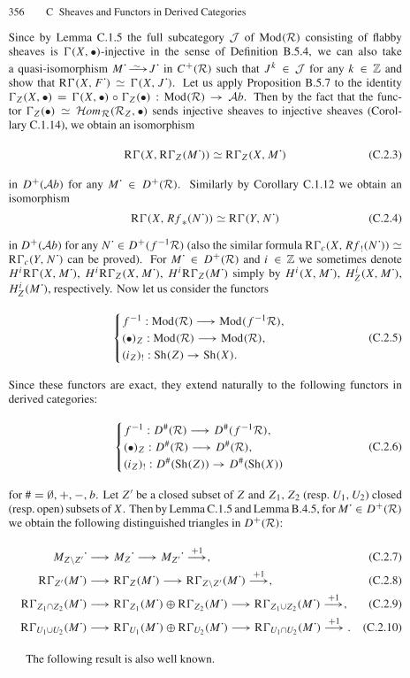
356 C Sheaves and Functors in Derived Categories
Since by Lemma C.1.5 the full subcategory J of Mod(R) consisting of flabbysheaves is �(X, •)-injective in the sense of Definition B.5.4, we can also take
a quasi-isomorphism M˙−→∼ J˙ in C+(R) such that J k ∈ J for any k ∈ Z andshow that R�(X, F˙) � �(X, J˙). Let us apply Proposition B.5.7 to the identity�Z(X, •) = �(X, •) ◦ �Z(•) : Mod(R) → Ab. Then by the fact that the func-tor �Z(•) � HomR(RZ, •) sends injective sheaves to injective sheaves (Corol-lary C.1.14), we obtain an isomorphism
R�(X, R�Z(M˙)) � R�Z(X, M˙) (C.2.3)
in D+(Ab) for any M˙ ∈ D+(R). Similarly by Corollary C.1.12 we obtain anisomorphism
R�(X, Rf ∗(N˙)) � R�(Y, N˙) (C.2.4)
in D+(Ab) for any N˙ ∈ D+(f −1R) (also the similar formula R�c(X, Rf !(N˙)) �R�c(Y, N˙) can be proved). For M˙ ∈ D+(R) and i ∈ Z we sometimes denoteHiR�(X, M˙), HiR�Z(X, M˙), HiR�Z(M˙) simply by Hi(X, M˙), Hi
Z(X, M˙),Hi
Z(M˙), respectively. Now let us consider the functors⎧⎪⎨⎪⎩f −1 : Mod(R) −→ Mod(f −1R),
(•)Z : Mod(R) −→ Mod(R),
(iZ)! : Sh(Z) → Sh(X).
(C.2.5)
Since these functors are exact, they extend naturally to the following functors inderived categories: ⎧⎪⎨⎪⎩
f −1 : D#(R) −→ D#(f −1R),
(•)Z : D#(R) −→ D#(R),
(iZ)! : D#(Sh(Z)) → D#(Sh(X))
(C.2.6)
for # = ∅, +, −, b. Let Z′ be a closed subset of Z and Z1, Z2 (resp. U1, U2) closed(resp. open) subsets of X. Then by Lemma C.1.5 and Lemma B.4.5, for M˙ ∈ D+(R)
we obtain the following distinguished triangles in D+(R):
MZ\Z′˙ −→ MZ˙ −→ MZ′˙ +1−→, (C.2.7)
R�Z′(M˙) −→ R�Z(M˙) −→ R�Z\Z′(M˙) +1−→, (C.2.8)
R�Z1∩Z2(M˙) −→ R�Z1(M˙) ⊕ R�Z2(M˙) −→ R�Z1∪Z2(M˙) +1−→, (C.2.9)
R�U1∪U2(M˙) −→ R�U1(M˙) ⊕ R�U2(M˙) −→ R�U1∩U2(M˙) +1−→ . (C.2.10)
The following result is also well known.
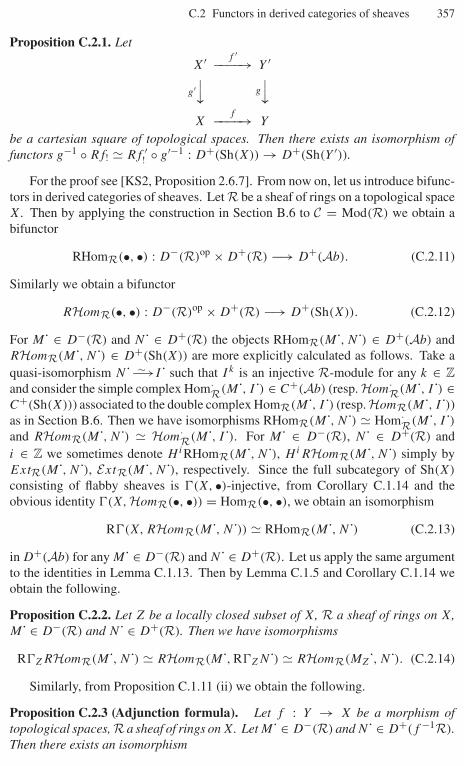
C.2 Functors in derived categories of sheaves 357
Proposition C.2.1. Let
X′ f ′−−−−→ Y ′
g′⏐⏐ g
⏐⏐X
f−−−−→ Y
be a cartesian square of topological spaces. Then there exists an isomorphism offunctors g−1 ◦ Rf! � Rf ′
! ◦ g′−1 : D+(Sh(X)) → D+(Sh(Y ′)).
For the proof see [KS2, Proposition 2.6.7]. From now on, let us introduce bifunc-tors in derived categories of sheaves. Let R be a sheaf of rings on a topological spaceX. Then by applying the construction in Section B.6 to C = Mod(R) we obtain abifunctor
RHomR(•, •) : D−(R)op × D+(R) −→ D+(Ab). (C.2.11)
Similarly we obtain a bifunctor
RHomR(•, •) : D−(R)op × D+(R) −→ D+(Sh(X)). (C.2.12)
For M˙ ∈ D−(R) and N˙ ∈ D+(R) the objects RHomR(M˙, N˙) ∈ D+(Ab) andRHomR(M˙, N˙) ∈ D+(Sh(X)) are more explicitly calculated as follows. Take aquasi-isomorphism N˙−→∼ I˙ such that I k is an injective R-module for any k ∈ Zand consider the simple complex Hom·
R(M˙, I˙) ∈ C+(Ab) (resp. Hom·R(M˙, I˙) ∈
C+(Sh(X))) associated to the double complex HomR(M˙, I˙) (resp. HomR(M˙, I˙))as in Section B.6. Then we have isomorphisms RHomR(M˙, N˙) � Hom·
R(M˙, I˙)and RHomR(M˙, N˙) � Hom·
R(M˙, I˙). For M˙ ∈ D−(R), N˙ ∈ D+(R) andi ∈ Z we sometimes denote HiRHomR(M˙, N˙), HiRHomR(M˙, N˙) simply byExtR(M˙, N˙), ExtR(M˙, N˙), respectively. Since the full subcategory of Sh(X)
consisting of flabby sheaves is �(X, •)-injective, from Corollary C.1.14 and theobvious identity �(X, HomR(•, •)) = HomR(•, •), we obtain an isomorphism
R�(X, RHomR(M˙, N˙)) � RHomR(M˙, N˙) (C.2.13)
in D+(Ab) for any M˙ ∈ D−(R) and N˙ ∈ D+(R). Let us apply the same argumentto the identities in Lemma C.1.13. Then by Lemma C.1.5 and Corollary C.1.14 weobtain the following.
Proposition C.2.2. Let Z be a locally closed subset of X, R a sheaf of rings on X,M˙ ∈ D−(R) and N˙ ∈ D+(R). Then we have isomorphisms
R�ZRHomR(M˙, N˙) � RHomR(M˙, R�ZN˙) � RHomR(MZ˙, N˙). (C.2.14)
Similarly, from Proposition C.1.11 (ii) we obtain the following.
Proposition C.2.3 (Adjunction formula). Let f : Y → X be a morphism oftopological spaces, R a sheaf of rings on X. Let M˙ ∈ D−(R) and N˙ ∈ D+(f −1R).Then there exists an isomorphism
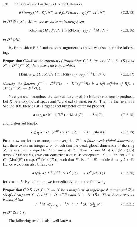
358 C Sheaves and Functors in Derived Categories
RHomR(M˙, Rf∗N˙) � Rf∗RHomf −1R(f −1M˙, N˙) (C.2.15)
in D+(Sh(X)). Moreover, we have an isomorphism
RHomR(M˙, Rf∗N˙) � RHomf −1R(f −1M˙, N˙) (C.2.16)
in D+(Ab).
By Proposition B.6.2 and the same argument as above, we also obtain the follow-ing.
Proposition C.2.4. In the situation of Proposition C.2.3, for any L˙ ∈ D+(R) andN˙ ∈ D+(f −1R) there exists an isomorphism
HomD+(R)(L˙, Rf∗N˙) � HomD+(f −1R)(f−1L˙, N˙). (C.2.17)
Namely, the functor f −1 : D+(R) → D+(f −1R) is a left adjoint of Rf∗ :D+(f −1R) → D+(R).
Next we shall introduce the derived functor of the bifunctor of tensor products.Let X be a topological space and R a sheaf of rings on X. Then by the results inSection B.6, there exists a right exact bifunctor of tensor products
• ⊗R • : Mod(Rop) × Mod(R) −→ Sh(X), (C.2.18)
and its derived functor
• ⊗LR • : D−(Rop) × D−(R) −→ D−(Sh(X)). (C.2.19)
From now on, let us assume, moreover, that R has finite weak global dimension,i.e., there exists an integer d > 0 such that the weak global dimension of the ringRx is less than or equal to d for any x ∈ X. Then for any M˙ ∈ C+(Mod(R))
(resp. Cb(Mod(R))) we can construct a quasi-isomorphism P ˙ → M˙ for P ˙ ∈C+(Mod(R)) (resp. Cb(Mod(R))) such that P k is a flat R-module for any k ∈ Z.Hence we obtain also bifunctors
• ⊗LR • : D#(Rop) × D#(R) −→ D#(Sh(X)) (C.2.20)
for # = +, b. By definition, we immediately obtain the following.
Proposition C.2.5. Let f : Y → X be a morphism of topological spaces and R asheaf of rings on X. Let M˙ ∈ D−(Rop) and N˙ ∈ D−(R). Then there exists anisomorphism
f −1M˙ ⊗Lf −1R f −1N˙ � f −1(M˙ ⊗L
R N˙) (C.2.21)
in D−(Sh(Y )).
The following result is also well known.
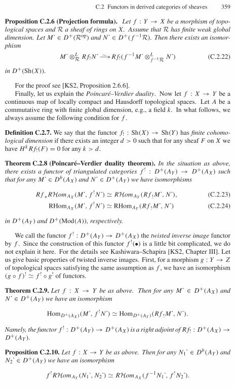
C.2 Functors in derived categories of sheaves 359
Proposition C.2.6 (Projection formula). Let f : Y → X be a morphism of topo-logical spaces and R a sheaf of rings on X. Assume that R has finite weak globaldimension. Let M˙ ∈ D+(Rop) and N˙ ∈ D+(f −1R). Then there exists an isomor-phism
M˙ ⊗LR Rf!N˙−→∼ Rf!(f −1M˙ ⊗L
f −1R N˙) (C.2.22)
in D+(Sh(X)).
For the proof see [KS2, Proposition 2.6.6].Finally, let us explain the Poincaré–Verdier duality. Now let f : X → Y be a
continuous map of locally compact and Hausdorff topological spaces. Let A be acommutative ring with finite global dimension, e.g., a field k. In what follows, wealways assume the following condition for f .
Definition C.2.7. We say that the functor f! : Sh(X) → Sh(Y ) has finite cohomo-logical dimension if there exists an integer d > 0 such that for any sheaf F on X wehave HkRf!(F ) = 0 for any k > d .
Theorem C.2.8 (Poincaré–Verdier duality theorem). In the situation as above,there exists a functor of triangulated categories f ! : D+(AY ) → D+(AX) suchthat for any M˙ ∈ Db(AX) and N˙ ∈ D+(AY ) we have isomorphisms
Rf ∗RHomAX(M˙, f !N˙) � RHomAY
(Rf !M˙, N˙), (C.2.23)
RHomAX(M˙, f !N˙) � RHomAY
(Rf !M˙, N˙) (C.2.24)
in D+(AY ) and D+(Mod(A)), respectively.
We call the functor f ! : D+(AY ) → D+(AX) the twisted inverse image functorby f . Since the construction of this functor f !(•) is a little bit complicated, we donot explain it here. For the details see Kashiwara–Schapira [KS2, Chapter III]. Letus give basic properties of twisted inverse images. First, for a morphism g : Y → Z
of topological spaces satisfying the same assumption as f , we have an isomorphism(g ◦ f )! � f ! ◦ g! of functors.
Theorem C.2.9. Let f : X → Y be as above. Then for any M˙ ∈ D+(AX) andN˙ ∈ D+(AY ) we have an isomorphism
HomD+(AX)(M˙, f !N˙) � HomD+(AY )(Rf !M˙, N˙).
Namely, the functor f ! : D+(AY ) → D+(AX) is a right adjoint of Rf! : D+(AX) →D+(AY ).
Proposition C.2.10. Let f : X → Y be as above. Then for any N1˙ ∈ Db(AY ) andN2˙ ∈ D+(AY ) we have an isomorphism
f !RHomAY(N1˙, N2˙) � RHomAX
(f −1N1˙, f !N2˙).
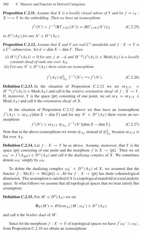
360 C Sheaves and Functors in Derived Categories
Proposition C.2.11. Assume that X is a locally closed subset of Y and let f = iX :X ↪−→ Y be the embedding. Then we have an isomorphism
f !(N˙) � f −1(R�f (X)(N˙)) = (R�f (X)(N˙))|X (C.2.25)
in D+(AX) for any N˙ ∈ D+(AY ).
Proposition C.2.12. Assume that X and Y are real C1-manifolds and f : X → Y isa C1-submersion. Set d = dim X − dim Y . Then
(i) Hj (f !(AY )) = 0 for any j = −d and H−d(f !(AY )) ∈ Mod(AX) is a locallyconstant sheaf of rank one over AX.
(ii) For any N˙ ∈ D+(AY ) there exists an isomorphism
f !(AY ) ⊗LAX
f −1(N˙) −→∼ f !(N˙). (C.2.26)
Definition C.2.13. In the situation of Proposition C.2.12 we set orX/Y =H−d(f !(AY )) ∈ Mod(AX) and call it the relative orientation sheaf of f : X → Y .If, moreover, Y is the space {pt} consisting of one point, we set orX = orX/Y ∈Mod(AX) and call it the orientation sheaf of X.
In the situation of Proposition C.2.12 above we thus have an isomorphismf !(AY ) � orX/Y [dim X − dim Y ] and for any N˙ ∈ D+(AY ) there exists an iso-morphism
f !(N˙) � orX/Y ⊗AXf −1(N˙)[dim X − dim Y ]. (C.2.27)
Note that in the above isomorphism we wrote ⊗AXinstead of ⊗L
AXbecause orX/Y is
flat over AX.
Definition C.2.14. Let f : X → Y be as above. Assume, moreover, that Y is thespace {pt} consisting of one point and the morphism f is X → {pt}. Then we setωX˙ = f !(A{pt}) ∈ D+(AX) and call it the dualizing complex of X. We sometimesdenote ωX˙ simply by ωX.
To define the dualizing complex ωX˙ ∈ D+(AX) of X, we assumed that thefunctor f! : Sh(X) → Sh({pt}) = Ab for f : X → {pt} has finite cohomologicaldimension. This assumption is satisfied if X is a topological manifold or a real analyticspace. In what follows we assume that all topological spaces that we treat satisfy thisassumption.
Definition C.2.15. For M˙ ∈ Db(AX) we set
DX(M˙) = RHomAX(M˙, ωX˙) ∈ D+(AX)
and call it the Verdier dual of M .
Since for the morphism f : X → Y of topological spaces we have f !ωY ˙ � ωX ,from Proposition C.2.10 we obtain an isomorphism
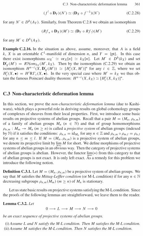
C.3 Non-characteristic deformation lemma 361
(f ! ◦ DY )(N˙) � (DX ◦ f −1)(N˙) (C.2.28)
for any N˙ ∈ Db(AY ). Similarly, from Theorem C.2.8 we obtain an isomorphism
(Rf ∗ ◦ DX)(M˙) � (DY ◦ Rf !)(M˙) (C.2.29)
for any M˙ ∈ Db(AX).
Example C.2.16. In the situation as above, assume, moreover, that A is a fieldk, X is an orientable C1-manifold of dimension n, and Y = {pt}. In this casethere exist isomorphisms ωX˙ � orX[n] � kX[n]. Let M˙ ∈ Db(kX) and setD′
X(M˙) = RHomkX(M˙, kX). Then by the isomorphism (C.2.29) we obtain an
isomorphism Hn−i (X, D′X(M˙)) � [Hi
c (X, M˙)]∗ for any i ∈ Z, where we setHi
c (X, •) = HiR�c(X, •). In the very special case where M˙ = kX we thus ob-tain the famous Poincaré duality theorem: Hn−i (X, kX) � [Hi
c (X, kX)]∗.
C.3 Non-characteristic deformation lemma
In this section, we prove the non-characteristic deformation lemma (due to Kashi-wara), which plays a powerful role in deriving results on global cohomology groupsof complexes of sheaves from their local properties. First, we introduce some basicresults on projective systems of abelian groups. Recall that a pair M = (Mn, ρn,m)
of a family of abelian groups Mn (n ∈ N) and that of group homomorphismsρn,m : Mm → Mn (m ≥ n) is called a projective system of abelian groups (indexedby N) if it satisfies the conditions: ρn,n = idMn for any n ∈ Z and ρn,m ◦ ρm,l = ρn,l
for any n ≤ m ≤ l. If M = (Mn, ρn,m) is a projective system of abelian groups,we denote its projective limit by lim←− M for short. We define morphisms of projectivesystems of abelian groups in an obvious way. Then the category of projective systemsof abelian groups is abelian. However, the functor lim←−(∗) from this category to thatof abelian groups is not exact. It is only left exact. As a remedy for this problem weintroduce the following notion.
Definition C.3.1. Let M = (Mn, ρn,m) be a projective system of abelian groups. Wesay that M satisfies the Mittag-Leffler condition (or M-L condition) if for any n ∈ Ndecreasing subgroups ρn,m(Mm) (m ≥ n) of Mn is stationary.
Let us state basic results on projective systems satisfying the M-Lcondition. Sincethe proofs of the following lemmas are straightforward, we leave them to the reader.
Lemma C.3.2. Let0 −→ L −→ M −→ N −→ 0
be an exact sequence of projective systems of abelian groups.
(i) Assume L and N satisfy the M-L condition. Then M satisfies the M-L condition.(ii) Assume M satisfies the M-L condition. Then N satisfies the M-L condition.
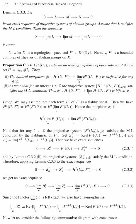
362 C Sheaves and Functors in Derived Categories
Lemma C.3.3. Let0 −→ L −→ M −→ N −→ 0
be an exact sequence of projective systems of abelian groups. Assume that L satisfiesthe M-L condition. Then the sequence
0 −→ lim←− L −→ lim←− M −→ lim←− N −→ 0
is exact.
Now let X be a topological space and F˙ ∈ Db(ZX). Namely, F˙ is a boundedcomplex of sheaves of abelian groups on X.
Proposition C.3.4. Let {Un}n∈N be an increasing sequence of open subsets of X andset U = ∪n∈NUn. Then
(i) The natural morphism φi : Hi(U, F˙) → lim←−n
H i(Un, F˙) is surjective for anyi ∈ Z.
(ii) Assume that for an integer i ∈ Z the projective system {Hi−1(Un, F˙)}n∈N sat-isfies the M-L condition. Then φi : Hi(U, F˙) → lim←−
n
H i(Un, F˙) is bijective.
Proof. We may assume that each term F i of F˙ is a flabby sheaf. Then we haveHi(U, F˙) = Hi(F˙(U)) = Hi(lim←−
n
F˙(Un)). Hence the morphism φi is
Hi(lim←−n
F˙(Un)) → lim←−n
H i(F˙(Un)).
Note that for any i ∈ Z the projective system {F i(Un)}n∈N satisfies the M-Lcondition by the flabbiness of F i . Set Zi
n = Ker[F i(Un) → F i+1(Un)] andBi
n = Im[F i−1(Un) → F i(Un)]. Then we have exact sequences
0 −→ Zin −→ F i(Un) −→ Bi+1
n −→ 0 (C.3.1)
and by Lemma C.3.2 (ii) the projective systems {Bin}n∈N satisfy the M-L condition.
Therefore, applying Lemma C.3.3 to the exact sequences
0 −→ Bin −→ Zi
n −→ Hi(Un, F˙) −→ 0 (C.3.2)
we get an exact sequence
0 −→ lim←−n
Bin −→ lim←−
n
Zin −→ lim←−
n
H i(Un, F˙) −→ 0. (C.3.3)
Since the functor lim←−(∗) is left exact, we also have isomorphisms
lim←−n
Zin � Ker[lim←−
n
F i(Un) → lim←−n
F i+1(Un)] = Ker[F i(U) → F i+1(U)].
Now let us consider the following commutative diagram with exact rows:
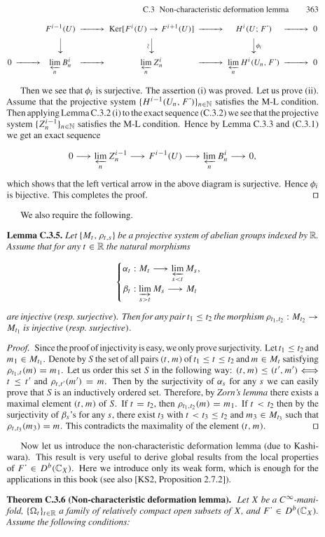
C.3 Non-characteristic deformation lemma 363
F i−1(U) −−−−→ Ker[F i(U) → F i+1(U)] −−−−→ Hi(U ; F˙) −−−−→ 0⏐⏐ �⏐⏐ ⏐⏐φi
0 −−−−→ lim←−n
Bin −−−−→ lim←−
n
Zin −−−−→ lim←−
n
Hi(Un, F˙) −−−−→ 0
Then we see that φi is surjective. The assertion (i) was proved. Let us prove (ii).Assume that the projective system {Hi−1(Un, F˙)}n∈N satisfies the M-L condition.Then applying Lemma C.3.2 (i) to the exact sequence (C.3.2) we see that the projectivesystem {Zi−1
n }n∈N satisfies the M-L condition. Hence by Lemma C.3.3 and (C.3.1)we get an exact sequence
0 −→ lim←−n
Zi−1n −→ F i−1(U) −→ lim←−
n
Bin −→ 0,
which shows that the left vertical arrow in the above diagram is surjective. Hence φi
is bijective. This completes the proof. ��We also require the following.
Lemma C.3.5. Let {Mt, ρt,s} be a projective system of abelian groups indexed by R.Assume that for any t ∈ R the natural morphisms⎧⎪⎨⎪⎩
αt : Mt −→ lim←−s<t
Ms,
βt : lim−→s>t
Ms −→ Mt
are injective (resp. surjective). Then for any pair t1 ≤ t2 the morphism ρt1,t2 : Mt2 →Mt1 is injective (resp. surjective).
Proof. Since the proof of injectivity is easy, we only prove surjectivity. Let t1 ≤ t2 andm1 ∈ Mt1 . Denote by S the set of all pairs (t, m) of t1 ≤ t ≤ t2 and m ∈ Mt satisfyingρt1,t (m) = m1. Let us order this set S in the following way: (t, m) ≤ (t ′, m′) ⇐⇒t ≤ t ′ and ρt,t ′(m′) = m. Then by the surjectivity of αs for any s we can easilyprove that S is an inductively ordered set. Therefore, by Zorn’s lemma there exists amaximal element (t, m) of S. If t = t2, then ρt1,t2(m) = m1. If t < t2 then by thesurjectivity of βs’s for any s, there exist t3 with t < t3 ≤ t2 and m3 ∈ Mt3 such thatρt,t3(m3) = m. This contradicts the maximality of the element (t, m). ��
Now let us introduce the non-characteristic deformation lemma (due to Kashi-wara). This result is very useful to derive global results from the local propertiesof F˙ ∈ Db(CX). Here we introduce only its weak form, which is enough for theapplications in this book (see also [KS2, Proposition 2.7.2]).
Theorem C.3.6 (Non-characteristic deformation lemma). Let X be a C∞-mani-fold, {�t }t∈R a family of relatively compact open subsets of X, and F˙ ∈ Db(CX).Assume the following conditions:
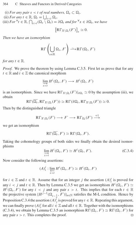
364 C Sheaves and Functors in Derived Categories
(i) For any pair s < t of real numbers, �s ⊂ �t .(ii) For any t ∈ R, �t = ⋃
s<t �s .(iii) For ∀t ∈ R,
⋂s>t (�s \ �t) = ∂�t and for ∀x ∈ ∂�t , we have[
R�X\�t (F˙)]x
� 0.
Then we have an isomorphism
R�
(⋃s∈R
�s, F˙)
−→∼ R�(�t , F˙)
for any t ∈ R.
Proof. We prove the theorem by using Lemma C.3.5. First let us prove that for anyt ∈ R and i ∈ Z the canonical morphism
lim−→s>t
H i(�s, F˙) −→ Hi(�t , F˙)
is an isomorphism. Since we have R�X\�t (F˙)|∂�t � 0 by the assumption (iii), weobtain
R�(�t , R�X\�t (F˙)) � R�(∂�t , R�X\�t (F˙)) � 0.
Then by the distinguished triangle
R�X\�t (F˙) −→ F˙ −→ R��t (F˙) +1−→we get an isomorphism
R�(�t , F˙) � R�(�t , F˙).Taking the cohomology groups of both sides we finally obtain the desired isomor-phisms
lim−→s>t
H i(�s, F˙) � Hi(�t , F˙). (C.3.4)
Now consider the following assertions:
(A)ti : lim←−
s<t
H i(�s, F˙) � Hi(�t , F˙)
for i ∈ Z and t ∈ R. Assume that for an integer j the assertion (A)ti is proved for
any i < j and t ∈ R. Then by Lemma C.3.5 we get an isomorphism Hi(�s, F˙) �Hi(�t , F˙) for any i < j and any pair s > t . This implies that for each t ∈ Rthe projective system {Hj−1(�
t− 1n, F˙)}n∈N satisfies the M-L condition. Hence by
Proposition C.3.4 the assertion (A)tj is proved for any t ∈ R. Repeating this argument,
we can finally prove (A)ti for all i ∈ Z and all t ∈ R. Together with the isomorphisms
(C.3.4), we obtain by Lemma C.3.5 an isomorphism R�(�s, F˙) � R�(�t , F˙) forany pair s > t . This completes the proof. ��
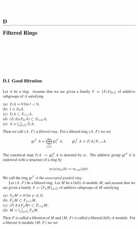
D
Filtered Rings
D.1 Good filtration
Let A be a ring. Assume that we are given a family F = {FlA}l∈Z of additivesubgroups of A satisfying
(a) FlA = 0 for l < 0,(b) 1 ∈ F0A,(c) FlA ⊂ Fl+1A,(d) (FlA)(FmA) ⊂ Fl+mA,(e) A = ⋃
l∈Z FlA.
Then we call (A, F ) a filtered ring. For a filtered ring (A, F ) we set
grF A =⊕l∈Z
grFl A, grF
l A = FlA/Fl−1A.
The canonical map FlA → grFl A is denoted by σl . The additive group grF A is
endowed with a structure of a ring by
σl(a)σm(b) = σl+m(ab).
We call the ring grF A the associated graded ring.Let (A, F ) be a filtered ring. Let M be a (left) A-module M , and assume that we
are given a family F = {FpM}p∈Z of additive subgroups of M satisfying
(a) FpM = 0 for p # 0,(b) FpM ⊂ Fp+1M ,(c) (FlA)(FpM) ⊂ Fl+pM ,(d) M = ⋃
p∈Z FpM .
Then F is called a filtration of M and (M, F ) is called a filtered (left) A-module. Fora filtered A-module (M, F ) we set
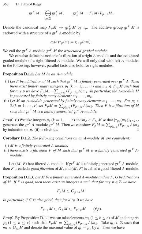
366 D Filtered Rings
grF M =⊕p∈Z
grFp M, grF
p M = FpM/Fp−1M.
Denote the canonical map FpM → grFp M by τp. The additive group grF M is
endowed with a structure of a grF A-module by
σl(a)τp(m) = τl+p(am).
We call the grF A-module grF M the associated graded module.We can also define the notion of a filtration of a right A-module and the associated
graded module of a right filtered A-module. We will only deal with left A-modulesin the following; however, parallel facts also hold for right modules.
Proposition D.1.1. Let M be an A-module.
(i) Let F be a filtration of M such that grF M is finitely generated over grF A. Thenthere exist finitely many integers pk (k = 1, . . . , r) and mk ∈ Fpk
M such thatfor any p we have FpM = ∑
p≥pk(Fp−pk
A)mk . In particular, the A-module M
is generated by finitely many elements m1, . . . , mk .(ii) Let M an A-module generated by finitely many elements m1, . . . , mk . For pk ∈
Z (k = 1, . . . , r) set FpM = ∑p≥pk
(Fp−pkA)mk . Then F is a filtration of M
such that grF M is a finitely generated grF A-module.
Proof. (i) We take integers pk (k = 1, . . . , r) and mk ∈ FpkM so that {τpk
(mk)}1≤k≤r
generates the grF A-module grF M . Then we can show FpM = ∑p≥pk
(Fp−pkA)mk
by induction on p. (ii) is obvious. ��Corollary D.1.2. The following conditions on an A-module M are equivalent:
(i) M is a finitely generated A-module,(ii) there exists a filtration F of M such that grF M is a finitely generated grF A-
module.
Let (M, F ) be a filtered A-module. If grF M is a finitely generated grF A-module,then F is called a good filtration of M , and (M, F ) is called a good filtered A-module.
Proposition D.1.3. Let M be a finitely generated A-module and let F, G be filtrationsof M . If F is good, then there exist an integers a such that for any p ∈ Z we have
FpM ⊂ Gp+aM.
In particular, if G is also good, then for a � 0 we have
Fp−aM ⊂ GpM ⊂ Fp+aM (∀p).
Proof. By Proposition D.1.1 we can take elements mk (1 ≤ k ≤ r) of M and integerspk (1 ≤ k ≤ r) such that FpM = ∑
p≥pk(Fp−pk
A)mk . Take qk ∈ Z such thatmk ∈ Gqk
M and denote the maximal value of qk − pk by a. Then we have
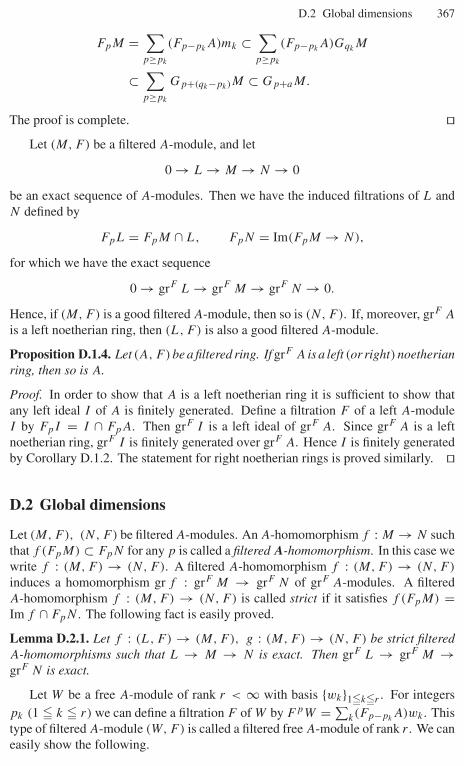
D.2 Global dimensions 367
FpM =∑
p≥pk
(Fp−pkA)mk ⊂
∑p≥pk
(Fp−pkA)Gqk
M
⊂∑
p≥pk
Gp+(qk−pk)M ⊂ Gp+aM.
The proof is complete. ��Let (M, F ) be a filtered A-module, and let
0 → L → M → N → 0
be an exact sequence of A-modules. Then we have the induced filtrations of L andN defined by
FpL = FpM ∩ L, FpN = Im(FpM → N),
for which we have the exact sequence
0 → grF L → grF M → grF N → 0.
Hence, if (M, F ) is a good filtered A-module, then so is (N, F ). If, moreover, grF A
is a left noetherian ring, then (L, F ) is also a good filtered A-module.
Proposition D.1.4. Let (A, F ) be a filtered ring. If grF A is a left (or right) noetherianring, then so is A.
Proof. In order to show that A is a left noetherian ring it is sufficient to show thatany left ideal I of A is finitely generated. Define a filtration F of a left A-moduleI by FpI = I ∩ FpA. Then grF I is a left ideal of grF A. Since grF A is a leftnoetherian ring, grF I is finitely generated over grF A. Hence I is finitely generatedby Corollary D.1.2. The statement for right noetherian rings is proved similarly. ��
D.2 Global dimensions
Let (M, F ), (N, F ) be filtered A-modules. An A-homomorphism f : M → N suchthat f (FpM) ⊂ FpN for any p is called a filtered A-homomorphism. In this case wewrite f : (M, F ) → (N, F ). A filtered A-homomorphism f : (M, F ) → (N, F )
induces a homomorphism gr f : grF M → grF N of grF A-modules. A filteredA-homomorphism f : (M, F ) → (N, F ) is called strict if it satisfies f (FpM) =Im f ∩ FpN . The following fact is easily proved.
Lemma D.2.1. Let f : (L, F ) → (M, F ), g : (M, F ) → (N, F ) be strict filteredA-homomorphisms such that L → M → N is exact. Then grF L → grF M →grF N is exact.
Let W be a free A-module of rank r < ∞ with basis {wk}1�k�r . For integerspk (1 � k � r) we can define a filtration F of W by F pW = ∑
k(Fp−pkA)wk . This
type of filtered A-module (W, F ) is called a filtered free A-module of rank r . We caneasily show the following.
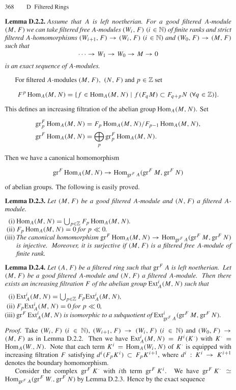
368 D Filtered Rings
Lemma D.2.2. Assume that A is left noetherian. For a good filtered A-module(M, F ) we can take filtered free A-modules (Wi, F ) (i ∈ N) of finite ranks and strictfiltered A-homomorphisms (Wi+1, F ) → (Wi, F ) (i ∈ N) and (W0, F ) → (M, F )
such that· · · → W1 → W0 → M → 0
is an exact sequence of A-modules.
For filtered A-modules (M, F ), (N, F ) and p ∈ Z set
F p HomA(M, N) = {f ∈ HomA(M, N) | f (FqM) ⊂ Fq+pN (∀q ∈ Z)}.This defines an increasing filtration of the abelian group HomA(M, N). Set
grFp HomA(M, N) = Fp HomA(M, N)/Fp−1 HomA(M, N),
grF HomA(M, N) =⊕
p
grFp HomA(M, N).
Then we have a canonical homomorphism
grF HomA(M, N) → HomgrF A(grF M, grF N)
of abelian groups. The following is easily proved.
Lemma D.2.3. Let (M, F ) be a good filtered A-module and (N, F ) a filtered A-module.
(i) HomA(M, N) = ⋃p∈Z Fp HomA(M, N).
(ii) Fp HomA(M, N) = 0 for p # 0.(iii) The canonical homomorphism grF HomA(M, N) → HomgrF A(grF M, grF N)
is injective. Moreover, it is surjective if (M, F ) is a filtered free A-module offinite rank.
Lemma D.2.4. Let (A, F ) be a filtered ring such that grF A is left noetherian. Let(M, F ) be a good filtered A-module and (N, F ) a filtered A-module. Then thereexists an increasing filtration F of the abelian group ExtiA(M, N) such that
(i) ExtiA(M, N) = ⋃p∈Z FpExtiA(M, N),
(ii) FpExtiA(M, N) = 0 for p # 0,(iii) grF ExtiA(M, N) is isomorphic to a subquotient of Exti
grF A(grF M, grF N).
Proof. Take (Wi, F ) (i ∈ N), (Wi+1, F ) → (Wi, F ) (i ∈ N) and (W0, F ) →(M, F ) as in Lemma D.2.2. Then we have ExtiA(M, N) = Hi(K ·) with K · =HomA(W·, N). Note that each term Ki = HomA(Wi, N) of K · is equipped withincreasing filtration F satisfying di(FpKi) ⊂ FpKi+1, where di : Ki → Ki+1
denotes the boundary homomorphism.Consider the complex grF K · with ith term grF Ki . We have grF K · �
HomgrF A(grF W·, grF N) by Lemma D.2.3. Hence by the exact sequence
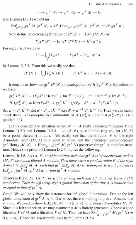
D.2 Global dimensions 369
· · · → grF W1 → grF W0 → grF M → 0,
(see Lemma D.2.1) we obtain
ExtigrF A(grF M, grF N) = Hi(HomgrF A(grF W·, grF N) � Hi(grF K ·).
Now define an increasing filtration of Hi(K ·) = ExtiA(M, N) by
FpHi(K ·) = Im(H i(F pK ·) → Hi(K ·)).For each i ∈ N we have
Ki =⋃p
FpKi, FpKi = 0 (p # 0).
by Lemma D.2.3. From this we easily see that
Hi(K ·) =⋃p
FpHi(K ·), FpH i(K ·) = 0 (p # 0).
It remains to show that grF H i(K ·) is a subquotient of Hi(grF K ·). By definitionwe have
grFp H i(K ·) = (FpKi ∩ Ker di + Im di−1)/(Fp−1Ki ∩ Ker di + Im di−1),
H i(grFp K ·) = Ker(FpKi → grF
p Ki+1)/(Fp−1Ki + di−1(FpKi−1)).
Set L = FpKi ∩ Ker di/(Fp−1Ki ∩ Ker di + di−1(FpKi−1)). Then we can easilycheck that L is isomorphic to a submodule of Hi(grF
p K ·) and that grFp H i(K ·) is a
quotient of L. ��Let us consider the situation where N = A (with canonical filtration F ) in
Lemma D.2.3 and Lemma D.2.4. Let (A, F ) be a filtered ring and let (M, F )
be a good filtered A-module. We easily see that the filtration F of the rightA-module HomA(M, A) is a good filtration and the canonical homomorphismgrF HomA(M, N) → HomgrF A(grF M, grF N) preserves the grF A-modules struc-ture. Hence (the proof of) Lemma D.2.4 implies the following.
Lemma D.2.5. Let (A, F ) be a filtered ring such that grF A is left noetherian, and let(M, F ) be a good filtered A-module. Then there exists a good filtration F of the rightA-module ExtiA(M, A) such that grF ExtiA(M, A) is isomorphic to a subquotient ofExti
grF A(grF M, grF A) as a right grF A-module.
Theorem D.2.6. Let (A, F ) be a filtered ring such that grF A is left (resp. right)noetherian. Then the left (resp. right) global dimension of the ring A is smaller thanor equal to that of grF A.
Proof. We will only show the statement for left global dimensions. Denote the leftglobal dimension of grF A by n. If n = ∞, there is nothing to prove. Assume thatn < ∞. We need to show ExtiA(M, N) = 0 (i > n) for arbitrary A-modules M, N .Since A is left noetherian, we may assume that M is finitely generated. Choose a goodfiltration F of M and a filtration F of N . Then we have Exti
grF A(grF M, grF N) =
0 (i > n). Hence the assertion follows from Lemma D.2.4. ��
370 D Filtered Rings
D.3 Singular supports
Let R be a commutative noetherian ring and let M be a finitely generated R-module.We denote by supp(M) the set of prime ideals p of R satisfying Mp = 0, and bysupp0(M) the set of minimal elements of supp(M). We have p ∈ supp(M) if andonly if p contains the annihilating ideal
AnnR(M) = {r ∈ R | rM = 0}.In fact, we have √
AnnR(M) =⋂
p∈supp(M)
p.
For p ∈ supp0(M) we denote the length of the artinian Rp-module Mp by 'p(M).We set 'q(M) = 0 for a prime ideal q ∈ supp(M). For an exact sequence
0 → L → M → N → 0
of finitely generated R-modules we have
supp(M) = supp(L) ∪ supp(N).
Moreover, for p ∈ supp0(M) we have
'p(M) = 'p(L) + 'p(N).
In the rest of this section (A, F ) denotes a filtered ring such that grF A is acommutative noetherian ring. Let M be a finitely generated A-module. By choosinga good filtration F we can consider supp(grF M) and 'p(grF M) for p ∈ supp0(M).
Lemma D.3.1. supp(grF M) and 'p(grF M) for p ∈ supp0(M) do not depend on thechoice of a good filtration F .
Proof. We say two good filtrations F and G are “adjacent’’if they satisfy the condition
FiM ⊂ GiM ⊂ Fi+1M (∀i ∈ Z).
We first show the assertion in this case. Consider the natural homomorphismϕi : FiM/Fi−1M → GiM/Gi−1M . Then we have Ker ϕi � Gi−1M/Fi−1M �Coker ϕi−1. Therefore, the morphism ϕ : grF M → grG M entails an isomorphismKer ϕ � Coker ϕ. Consider the exact sequence
0 → Ker ϕ → grF Mϕ→ grG M → Coker ϕ → 0
of finitely generated grF A-modules. From this we obtain
supp(grF M) = supp(Ker ϕ) ∪ supp(Im ϕ),
supp(grG M) = supp(Im ϕ) ∪ supp(Coker ϕ).

D.3 Singular supports 371
Hence Ker ϕ � Coker ϕ implies supp(grF M) = supp(grG M). Moreover, for p ∈supp0(grF M) = supp0(grG M) we have
'p(grF M) = 'p(Ker ϕ) + 'p(Im ϕ) = 'p(grG M).
The assertion is proved for adjacent good filtrations.Let us consider the general case. Namely, assume that F and G are arbitrary good
filtrations of M . For k ∈ Z set
F(k)i M = FiM + Gi+kM (i ∈ Z).
By Proposition D.1.3 F (k) is a good filtration of M satisfying the conditions⎧⎪⎨⎪⎩F (k) = F (k # 0),
F (k) = G[k] (k � 0),
F (k) and F (k+1) are adjacent,
where G[k] is a filtration obtained form G by the degree shift [k]. Therefore, ourassertion follows form the adjacent case. ��Definition D.3.2. For a finitely generated A-module M we set
SS(M) = supp(grF M),
SS0(M) = supp0(grF M),
JM =√
AnngrF A(grF M) =⋂
p∈SS0(M)
p,
d(M) = Krull dim(
grF A/JM
),
mp(M) = 'p(grF M) (p ∈ SS0(M) or p /∈ SS(M)),
where F is a good filtration of M . SS(M) and JM are called the singular supportand the characteristic ideal of M , respectively.
Lemma D.3.3. For an exact sequence
0 → L → M → N → 0
of finitely generated A-modules we have
SS(M) = SS(L) ∪ SS(N),
d(M) = max{d(L), d(N)},mp(M) = mp(L) + mp(N) (p ∈ SS0(M)).
Proof. Take a good filtration F of M . With respect to the induced filtrations of L andN we have a short exact sequence
0 −→ grF M −→ grF N −→ grF L −→ 0.
Hence the assertions for SS and 'p are obvious. The assertion for d follows from theone for SS. ��
372 D Filtered Rings
Since grF A is commutative, we have [FpA, FqA] ⊂ Fp+q−1A. Here, for a, b ∈A we set [a, b] = ab − ba. Hence we obtain a bi-additive product
{ , } : grFp A × grF
q A → grFp+q−1 A, ({σp(a), σq(b)} = σp+q−1([a, b])).
Its bi-additive extension
{ , } : grF A × grF A → grF A
is called the Poisson bracket. It satisfies the following properties:
(i) {a, b} + {b, a} = 0,(ii) {{a, b}, c} + {{b, c}, a} + {{c, a}, b} = 0,
(iii) {a, bc} = {a, b}c + b{a, c}.We say that an ideal I of grF A is involutive if it satisfies {I, I } ⊂ I .
We state the following deep result of Gabber [Ga] without proof.
Theorem D.3.4. Assume that (A, F ) is a filtered ring such that the center of A con-tains a subring isomorphic to Q and that grF A is a commutative noetherian ring.Let M be a finitely generated A-module. Then any p ∈ SS0(M) is involutive. Inparticular, JM is involutive.
D.4 Duality
In this section (A, F ) is a filtered ring such that grF A is a regular commutative ringof pure dimension m (a commutative ring R is called a regular ring of pure dimensionm if its localization at any maximal ideal is a regular local ring of dimension m). Inparticular, grF A is a noetherian ring whose global dimension and Krull dimensionare equal to m. Hence A is a left and right noetherian ring with global dimension� m by Proposition D.1.4 and Theorem D.2.6. We will consider properties of theExt-groups ExtiA(M, A) for finitely generated A-modules M .
Note first that for any (left) A-module M the Ext-groups ExtiA(M, A) are endowedwith a right A-module structure (i.e., a left Aop-module structure, where Aop denotesthe opposite ring) by the right multiplication of A on A. Since A has global dimension� m, we have ExtiA(M, A) = 0 for i > m. Moreover, if M is finitely generated, thenExtiA(M, A) are also finitely generated since A is left noetherian.
Let us give a formulation in terms of the derived category. Let Mod(A) andModf (A) denote the category of (left) A-modules and its full subcategory consistingof finitely generated A-modules, respectively. Denote by Db(A) and Db
f (A) thebounded derived category of Mod(A) and its full subcategory consisting of complexeswhose cohomology groups belong to Modf (A). Our objectives are the functors
D = R HomA(•, A) : Dbf (A) → Db
f (Aop)op,
D′ = R HomAop(•, Aop) : Dbf (Aop) → Db
f (A)op,
where Dbf (Aop) is defined similarly.

D.4 Duality 373
Proposition D.4.1. We have D′ ◦ D � Id and D ◦ D′ � Id.
Proof. By symmetry we have only to show D′◦D � Id. We first construct a canonicalmorphism M · → D′DM · for M · ∈ Db
f (A). Set H · = DM · = R HomA(M ·, A). By
R HomA⊗ZAop(M · ⊗Z H ·, A) � R HomA(M ·, R HomAop(H ·, Aop))
we have
HomA⊗ZAop(M · ⊗Z H ·, A) � HomA(M ·, R HomAop(H ·, Aop))
Hence the canonical morphism M · ⊗Z H ·(= M · ⊗Z R HomA(M ·, A)) → A inDb(A ⊗Z Aop) gives rise to a canonical morphism
M · → R HomAop(H ·, Aop)(= D′DM)
in Db(A). It remains to show that M · → D′DM · is an isomorphism. By taking a freeresolution of M · we may replace M · with A. In this case the assertion is clear. ��
For M · ∈ Dbf (A) (or Db
f (Aop)) we set
SS(M ·) =⋃
i
SS(H i(M ·)).
We easily see by Lemma D.3.3 that for a distinguished triangle
L· −→ M · −→ N · +1−→we have SS(M ·) ⊂ SS(L·) ∪ SS(N ·).
Proposition D.4.2. For M · ∈ Dbf (A) (resp. Db
f (Aop)) we have SS(DM ·) = SS(M ·)(resp. SS(D′M ·) = SS(M ·)).
Proof. By Proposition D.4.1 and symmetry we have only to show SS(DM ·) ⊂SS(M ·) for M · ∈ Db
f (A). We use induction on the cohomological length of M ·.We first consider the case where M · = M ∈ Modf (A). Take a good filtrationF of M and consider a good filtration F of ExtiA(M, A) as in Lemma D.2.5. ByLemma D.2.5 we have
SS(ExtiA(M, A)) = supp(grF ExtiA(M, A)) ⊂ supp(ExtigrF A(grF M, grF A))
⊂ supp(grF M) = SS(M).
The assertion is proved in the case where M · = M ∈ Modf (A). Now we considerthe general case. Set k = min{i | Hi(M ·) = 0}. Then we have a distinguishedtriangle
Hk(M ·)[−k] −→ M · −→ N · +1−→,
where N · = τ�k+1M ·. By
374 D Filtered Rings
Hi(N ·) ={
Hi(M ·) (i = k)
0 (i = k)
we obtain SS(M ·) = SS(N ·) ∪ SS(Hk(M ·)). Moreover, by the hypothesis of induc-tion we have SS(DN ·) ⊂ SS(N ·) and SS(DHk(M ·)) ⊂ SS(Hk(M ·)). Hence by thedistinguished triangle
DN · −→ DM · −→ (DHk(M ·))[k] +1−→we obtain
SS(DM ·) ⊂ SS(DHk(M ·)) ∪ SS(DN ·) ⊂ SS(Hk(M ·)) ∪ SS(N ·) = SS(M ·).
The proof is complete. ��For a finitely generated A-module M set
j (M) := min{i | ExtiA(M, A) = 0}.Theorem D.4.3. Let M be a finitely generated A-module.
(i) j (M) + d(M) = m,(ii) d(ExtiA(M, A)) ≤ m − i (i ∈ Z),
(iii) d(Extj (M)A (M, A)) = d(M).
(Recall that m denotes the global dimension of grF A.)
The following corresponding fact for regular commutative rings is well known(see [Ser2], [Bj1]).
Theorem D.4.4. Let R be a regular commutative ring of dimension m′. For afinitely generated R-module N we set d(N) := Krull dim(R/ AnnR N) and j (N) :=min{ i | ExtiR(N, R) = 0}.
(i) d(N) + j (N) = m′,(ii) d(ExtiR(N, R)) ≤ m′ − i (i ∈ Z),
(iii) d(Extj (N)R (N, R)) = d(N).
Proof of Theorem D.4.3. We apply Theorem D.4.4 to the case R = grF A. Fixa good filtration F of M . By Lemma D.2.4 (iii) we have SS(ExtiA(M, A)) ⊂supp(Exti
grF A(grF M, grF A)) and hence
d(ExtiA(M, A)) � d(ExtigrF A(grF M, grF A)).
Thus (ii) follows from the corresponding fact for grF A. Moreover, we haveExtiA(M, A) = 0 for i < j (grF M). Hence in order to show (i) and (iii) it issufficient to verify

D.5 Codimension filtration 375
d(Extj (grF M)
A (M, A)) = d(M).
By Proposition D.4.2 we have
d(M) = maxi�j (grF M)
d(ExtiA(M, A)).
For i > j (grF M) we have
d(ExtiA(M, A)) � m − i < m − j (grF M) = d(grF M) = d(M),
and hence we must have d(Extj (grF M)
A (M, A)) = d(M). ��Corollary D.4.5. For an exact sequence
0 → L → M → N → 0
of finitely generated A-modules we have
j (M) = min{j (L), j (N)}.
D.5 Codimension filtration
In this section (A, F ) is a filtered ring such that grF A is a regular commutative ringof pure dimension m. For a finitely generated A-module M and s ≥ 0 we denoteby Cs(M) the sum of all submodules N of M satisfying j (N) ≥ s. Since Cs(M)
is finitely generated, we have j (Cs(M)) ≥ s by Corollary D.4.5 and hence Cs(M)
is the largest submodule N of M satisfying j (N) ≥ s. By definition we have adecreasing filtration
0 = Cm+1(M) ⊂ Cm(M) ⊂ · · · ⊂ C1(M) ⊂ C0(M) = M.
We say that a finitely generated A-module M is purely s-codimensional if Cs(M) =M and Cs+1(M) = 0.
Lemma D.5.1. For any finitely generated A-module M Cs(M)/Cs+1(M) is purelys-codimensional.
Proof. Set N = Cs(M)/Cs+1(M). Then we have j (N) ≥ j (Cs(M)) ≥ s and henceCs(N) = N . Set K = Ker (Cs(M) → N/Cs+1(N)). Then by the exact sequence
0 → Cs+1(M) → K → Cs+1(N) → 0
we have j (K) = min{j (Cs+1(M)), j (Cs+1(N))} ≥ s + 1. By the maximality ofCs+1(M) we obtain K = Cs+1(M), i.e., Cs+1(N) = 0. ��
376 D Filtered Rings
We will give a cohomological interpretation of this filtration.For a finitely generated A-module M and s ≥ 0 we set
T s(M) = Ext0Aop(τ
�sR HomA(M, A), Aop).
By Proposition D.4.1 we have T 0(M) = M . By j (Exts(M, A)) ≥ s we haveExts−1
Aop (Exts(M, A), Aop) = 0. Hence by applying R HomAop(•, Aop) to the distin-guished triangle
ExtsA(M, A)[−s] −→ τ�sR HomA(M, A) −→ τ�s+1R HomA(M, A)+1−→
and taking the cohomology groups we obtain an exact sequence
0 → T s+1(M) → T s(M) → ExtsAop(ExtsA(M, A), Aop).
Hence we obtain a decreasing filtration
0 = T m+1(M) ⊂ T m(M) ⊂ · · · ⊂ T 1(M) ⊂ T 0(M) = M.
Proposition D.5.2. For any s we have Cs(M) = T s(M).
Proof. By j (ExtsAop(Exts(M, A), Aop)) ≥ s we see from the exact sequence
0 → T s+1(M) → T s(M) → ExtsAop(ExtsA(M, A), Aop)
using the backward induction on s that j (T s(M)) ≥ s. Hence T s(M) ⊂ Cs(M). Itremains to show the opposite inclusion. Set N = Cs(M). By j (N) ≥ s we have
τ�sR HomA(N, A) = R HomA(N, A),
and hence N = T s(N). By the functoriality of T s we have a commutative diagram
T s(N) N⏐⏐ ⏐⏐T s(M) −−−−→ M,
which implies N ⊂ T s(M). ��Theorem D.5.3. Let M be a finitely generated A-module which is purely s-codimen-sional. Then for any p ∈ SS0(M) we have
Krull dim((grF A)/p) = m − s.
Proof. The assertion being trivial for M = 0 we assume that M = 0. In this case wehave j (M) = s. Let F be a good filtration of M . Then there exists a good filtrationF of N = ExtsA(M, A) such that grF N is a subquotient of Exts
grF A(grF M, grF A).
Hence
D.5 Codimension filtration 377
SS(N) = supp(grF N) ⊂ supp(ExtsgrF A(grF M, grF A))
⊂ supp(grF M) = SS(M).
On the other hand since M is purely s-codimensional, we have
M = T s(M)/T s+1(M) ⊂ ExtsAop(ExtsA(M, A), Aop) = ExtsAop(N, Aop)
and hence SS(M) ⊂ SS(ExtsAop(N, Aop)) ⊂ SS(N). Therefore, we have
SS(M) = supp(grF M) = supp(ExtsgrF A(grF M, grF A)).
By j (grF M) = j (M) = s we have j ((grF A)/p) ≥ s for any p ∈ supp0(grF M).Set � = {p ∈ supp0(grF M) | j ((grF A)/p) = s)}. By a well-known fact incommutative algebra there exists a submodule L of grF M such that j (L) > s andsupp0(grF M/L) = �. We need to show supp(grF M) = supp(grF M/L). We haveobviously supp(grF M) ⊃ supp(grF M/L). On the other hand by Exts(L, grF A) =0 we have an injection Exts(grF M, grF A) → Exts(grF M/L, grF A), and hence
supp(grF M) = supp(Exts(grF M, grF A)) ⊂ supp(Exts(grF M/L, grF A))
⊂ supp(grF M/L).
The proof is complete. ��
E
Symplectic Geometry
In this chapter we first present basic results in symplectic geometry laying specialemphasis on cotangent bundles of complex manifolds. Most of the results are wellknown and we refer the reader to Abraham–Mardsen [AM] and Duistermaat [Dui]for details. Next we will precisely study conic Lagrangian analytic subsets in thecotangent bundles of complex manifolds. We prove that such a Lagrangian subset iscontained in the union of the conormal bundles of strata in a Whitney stratificationof the base manifold (Kashiwara’s theorem in [Kas3], [Kas8]).
E.1 Symplectic vector spaces
Let V be a finite-dimensional vector space over a field k. A symplectic form σ on V isa non-degenerate anti-symmetric bilinear form on V . If a vector space V is endowedwith a symplectic form σ , we call the pair (V , σ ) a symplectic vector space. Thedimension of a symplectic vector space is even. Let (V , σ ) be a symplectic vectorspace. Denote by V ∗ the dual of V . Then for any θ ∈ V ∗ there exists a uniqueHθ ∈ V such that
< θ, v >= σ(v, Hθ ) (v ∈ V )
by the non-degeneracy of σ . The correspondence θ �→ Hθ defines the Hamiltonianisomorphism H : V ∗ � V . For a linear subspace W of V consider its orthogonalcomplement W⊥ = {v ∈ V |σ(v, W) = 0} with respect to σ . Then again by thenon-degeneracy of σ we obtain dim W + dim W⊥ = dim V . Now let us introducethe following important linear subspaces of V .
Definition E.1.1. A linear subspace W of V is called isotropic (resp. Lagrangian,resp. involutive) if it satisfies W ⊂ W⊥ (resp. W = W⊥, resp. W ⊃ W⊥).
Note that if a linear subspace W ⊂ V is isotropic (resp. Lagrangian, resp. invo-lutive) then dim W ≤ 1
2 dim V (resp. dim W = 12 dim V , resp. dim W ≥ 1
2 dim V ).Moreover, a one-dimensional subspace (resp. a hyperplane) of V is always isotropic(resp. involutive).
380 E Symplectic Geometry
Example E.1.2. Let W be a finite-dimensional vector space and W ∗ its dual. SetV = W ⊕ W ∗ and define a bilinear form σ on V by
σ((x, ξ), (x′, ξ ′)) =< x′, ξ > − < x, ξ ′ > ((x, ξ), (x′, ξ ′) ∈ V = W ⊕ W ∗).
Then (V , σ ) is a symplectic vector space. Moreover, W and W ∗ are Lagrangiansubspaces of V .
E.2 Symplectic structures on cotangent bundles
A complex manifold X is called a (holomorphic) symplectic manifold if there existsa holomorphic 2-form σ globally defined on X which induces a symplectic form onthe tangent space TxX of X at each x ∈ X. The dimension of a symplectic manifoldis necessarily even. As one of the most important examples of symplectic manifolds,we treat here cotangent bundles of complex manifolds.
Now let X be a complex manifold and T X (resp. T ∗X) its tangent (resp. cotangent)bundle. We denote by π : T ∗X → X the canonical projection. By differentiatingπ we obtain the tangent map π ′ : T (T ∗X) → (T ∗X) ×X (T X) and its dual ρπ :(T ∗X) ×X (T ∗X) → T ∗(T ∗X). If we restrict ρπ to the diagonal T ∗X of (T ∗X) ×X
(T ∗X) then we get a map T ∗X → T ∗(T ∗X). Since this map is a holomorphic sectionof the bundle T ∗(T ∗X) → T ∗X, it corresponds to a (globally defined) holomorphic1-form αX on T ∗X. We call αX the canonical 1-form. If we take a local coordinate(x1, x2, . . . , xn) of X on an open subset U ⊂ X, then any point p of T ∗U ⊂ T ∗X
can be written uniquely as p = (x1, x2, . . . , xn; ξ1dx1 + ξ2dx2 + · + ξndxn) whereξi ∈ C. We call (x1, x2, . . . , xn; ξ1, ξ2, . . . , ξn) the local coordinate system of T ∗X
associated to (x1, x2, . . . , xn). In this local coordinate of T ∗X the canonical 1-formαX is written as αX = ∑n
i=1 ξidxi . Set σX = dαX = ∑ni=1 dξi ∧ dxi . Then we see
that the holomorphic 2-form σX defines a symplectic structure on Tp(T ∗X) at eachpoint p ∈ T ∗X. Namely, the cotangent bundle T ∗X is endowed with a structure ofa symplectic manifold by σX. We call σX the (canonical) symplectic form of T ∗X.Since there exists the Hamiltonian isomorphism H : T ∗
p (T ∗X) � Tp(T ∗X) at eachp ∈ T ∗X, we obtain the global isomorphism H : T ∗(T ∗X) � T (T ∗X). For aholomorphic function f on T ∗X we define a holomorphic vector field Hf to be theimage of the 1-form df by H : T ∗(T ∗X) � T (T ∗X). The vector field Hf is calledthe Hamiltonian vector field of f . Define the Poisson bracket of two holomorphicfunctions f, g on T ∗X by {f, g} = Hf (g) = σX(Hf , Hg). In the local coordinate(x1, x2, . . . , xn; ξ1, ξ2, . . . , ξn) of T ∗X we have the explicit formula
Hf =n∑
i=1
(∂f
∂ξi
∂
∂xi
− ∂f
∂xi
∂
∂ξi
).
We can also easily verify the following:⎧⎪⎨⎪⎩{f, g} = −{g, f },{f, hg} = h{f, g} + g{f, h},{{f, g}, h} + {{g, h}, f } + {{h, f }, g} = 0.
E.3 Lagrangian subsets of cotangent bundles 381
Moreover, we have [Hf , Hg] = H{f,g}, where [Hf , Hg] is the Lie bracket of Hf
and Hg .
Definition E.2.1. An analytic subset V of T ∗X is called isotropic (resp. Lagrangian,resp. involutive) if for any smooth point p ∈ Vreg of V the tangent space TpV at p isa isotropic (resp. a Lagrangian, resp. an involutive) subspace in Tp(T ∗X).
By definition the dimension of a Lagrangian analytic subset of T ∗X is equal todim X.
Example E.2.2.(i) Let Y ⊂ X be a complex submanifold of X. Then the conormal bundle T ∗
Y X ofY in X is a Lagrangian submanifold of T ∗X.
(ii) Let f be a holomorphic function on X. Set �f = {(x, grad f (x)|x ∈ X}. Then�f is a Lagrangian submanifold of T ∗X.
For an analytic subset V of T ∗X denote by IV the subsheaf of OT ∗X consistingof holomorphic functions vanishing on V .
Lemma E.2.3. For an analytic subset V of T ∗X the following conditions are equiv-alent:
(i) V is involutive.(ii) {IV , IV } ⊂ IV .
Proof. By the definition of Hamiltonian isomorphisms, for each smooth point p ∈Vreg of V the orthogonal complement (TpV )⊥ of TpV in the symplectic vector spaceTp(T ∗X) is spanned by the Hamiltonian vector fields Hf of f ∈ IV . Assume that V
is involutive. If f, g ∈ IV then the Hamiltonian vector field Hf is tangent to Vreg andhence {f, g} = Hf (g) = 0 on Vreg. Since {f, g} is holomorphic and Vreg is dense inV , {f, g} = 0 on the whole V , i.e., {f, g} ∈ IV . The part (i) =⇒ (ii) was proved.The converse can be proved more easily. ��
E.3 Lagrangian subsets of cotangent bundles
Let X be a complex manifold of dimension n. Since the fibers of the cotangent bundleT ∗X are complex vector spaces, there exists a natural action of the multiplicativegroup C× = C \ {0} on T ∗X. We say that an analytic subset V of T ∗X is conic ifV is stable by this action of C×. In this subsection we focus our attention on conicLagrangian analytic subsets of T ∗X.
First let us examine the image H(αX) of the canonical 1-form αX by theHamiltonian isomorphism H : T ∗(T ∗X) � T (T ∗X). In a local coordinate(x1, x2, . . . , xn; ξ1, ξ2, . . . , ξn) of T ∗X the holomorphic vector field H(αX) thus ob-tained has the form
H(αX) = −n∑
i=1
ξi
∂
∂ξi
.
It follows that −H(αX) is the infinitesimal generator of the action of C× on T ∗X.We call this vector field the Euler vector field .
382 E Symplectic Geometry
Lemma E.3.1. Let V be a conic complex submanifold of T ∗X. Then V is isotropicif and only if the pull-back αX|V of αX to V is identically zero.
Proof. Assume that αX|V is identically zero on V . Then also the pull-back of thesymplectic 2-form σX = dαX to V vanishes. Hence V is isotropic. Let us prove theconverse. Assume that V is isotropic. Then for any local section δ of the tangentbundle T V → V we have
〈αX, δ〉 = σX(δ, H(αX)) = 0
on V because the Euler vector field −H(αX) is tangent to V by the conicness of V .This means that αX|V is identically zero on V . ��Corollary E.3.2. Let � be a conic Lagrangian analytic subset of T ∗X. Then thepull-back of αX to the regular part �reg of � is identically zero.
Let Z be an analytic subset of the base space X and denote by T ∗Zreg
X the closureof the conormal bundle T ∗
ZregX of Zreg in T ∗X. Since the closure is taken with respect
to the classical topology of T ∗X, it is not clear if T ∗Zreg
X is an analytic subset of T ∗X
or not. In Proposition E.3.5 below, we will prove the analyticity of T ∗Zreg
X. For thispurpose, recall the following definitions.
Definition E.3.3. Let S be an analytic space. A locally finite partition S = ⊔α∈A Sα
of S by locally closed complex manifolds Sα’s is called a stratification of S if for eachSα the closure Sα and the boundary ∂Sα = Sα \ Sα are analytic and unions of Sβ ’s.A complex manifold Sα in it is called a stratum of the stratification S = ⊔
α∈A Sα .
Definition E.3.4. Let S be an analytic space. Then we say that a subset S′ of S isconstructible if there exists stratification S = ⊔
α∈A Sα of S such that S′ is a unionof some strata in it.
For an analytic space S the family of constructible subsets of S is closed undervarious set-theoretical operations. Note also that by definition the closure of a con-structible subset is analytic. Moreover, if f : S → S′ is a morphism (resp. propermorphism) of analytic spaces, then the inverse (resp. direct) image of a constructiblesubset of S′ (resp. S) by f is again constructible. Now we are ready to prove thefollowing.
Proposition E.3.5. T ∗Zreg
X is an analytic subset of T ∗X.
Proof. We may assume that Z is irreducible. By Hironaka’s theorem there exists aproper holomorphic map f : Y → X from a complex manifold Y and an analyticsubset Z′ = Z of Z such that f (Y ) = Z, Z0 := Z\Z′ is smooth, and the restriction off to Y0 := f −1(Z0) induces a biholomorphic map f |Y0 : Y0 � Z0. From f : Y → X
we obtain the canonical morphisms
T ∗Yρf←−−−−− Y ×X T ∗X
�f−−−−−→ T ∗X.

E.3 Lagrangian subsets of cotangent bundles 383
We easily see that T ∗Z0
X = �f ρ−1f (T ∗
Y0Y0), where T ∗
Y0Y0 � Y0 is the zero-section of
T ∗Y0 ⊂ T ∗Y . Since T ∗Y0
Y0 is a constructible subset of T ∗Y and �f is proper, T ∗Z0
X
is a constructible subset of T ∗X. Hence the closure T ∗Z0
X = T ∗Zreg
X is an analyticsubset of T ∗X. ��
By Example E.2.2 and Proposition E.3.5, for an irreducible analytic subset Z of X
we conclude that the closure T ∗Zreg
X is an irreducible conic Lagrangian analytic subsetof T ∗X. The following result, which was first proved by Kashiwara [Kas3], [Kas8],shows that any irreducible conic Lagrangian analytic subset of T ∗X is obtained inthis way.
Theorem E.3.6 (Kashiwara [Kas3], [Kas8]). Let � be a conic Lagrangian analyticsubset of T ∗X. Assume that � is irreducible. Then Z = π(�) is an irreducibleanalytic subset of X and � = T ∗
ZregX.
Proof. Since � is conic, Z = π(�) = (T ∗XX) ∩ � is an analytic subset of X.
Moreover, by definition we easily see that Z is irreducible. Denote by �0 the opensubset of π−1(Zreg)∩�reg consisting of points where the map π |�reg has the maximalrank. Then �0 is open dense in π−1(Zreg)∩� and the maximal rank is equal to dim Z.Now let p be a point in �0. Taking a local coordinate (x1, x2, . . . , xn) of X aroundthe point π(p) ∈ Zreg, we may assume that Z = {x1 = x2 = · · · = xd = 0} whered = n − dim Z. Let us choose a local section s : Zreg ↪→ �reg of π |�reg such thats(π(p)) = p. Let i�reg : �reg ↪→ T ∗X be the embedding. Then by Corollary E.3.2the pull-back of the canonical 1-form αX to Zreg by i�reg ◦ s is zero. On the otherhand, this 1-form on Zreg has the form ξd+1(x′)dxd+1 + · · · + ξn(x′)dxn, where weset x′ = (xd+1, . . . , xn). Therefore, the point p should be contained in {ξd+1 =· · · = ξn = 0}. We proved that �0 ⊂ T ∗
ZregX. Since dim �0 = dim T ∗
ZregX = n we
obtain T ∗Zreg
X = �0 ⊂ �. Then the result follows from the irreducibility of �. ��To treat general conic Lagrangian analytic subsets of T ∗X let us briefly explain
Whitney stratifications.
Definition E.3.7. Let S be an analytic subset of a complex manifold M . A stratifica-tion S = ⊔
α∈A Sα of S is called a Whitney stratification if it satisfies the followingWhitney conditions (a) and (b):
(a) Assume that a sequence xi ∈ Sα of points converges to a point y ∈ Sβ (α = β)and the limit T of the tangent spaces Txi
Sα exists. Then we have TySβ ⊂ T .(b) Let xi ∈ Sα and yi ∈ Sβ be two sequences of points which converge to the same
point y ∈ Sβ (α = β). Assume further that the limit l (resp. T ) of the lines lijointing xi and yi (resp. of the tangent spaces Txi
Sα) exists. Then we have l ⊂ T .
It is well known that any stratification of an analytic set can be refined to satisfy theWhitney conditions. Intuitively, the Whitney conditions means that the geometricalnormal structure of the stratification S = ⊔
α∈A Sα is locally constant along eachstratum Sα as is illustrated in the example below.
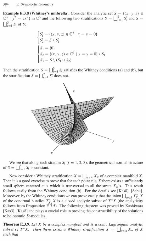
384 E Symplectic Geometry
Example E.3.8 (Whitney’s umbrella). Consider the analytic set S = {(x, y, z) ∈C3 | y2 = zx2} in C3 and the following two stratifications S = ⊔2
i=1 S′i and S =⊔3
i=1 Si of S: {S′
1 = {(x, y, z) ∈ C3 | x = y = 0}S′
2 = S \ S′1⎧⎪⎨⎪⎩
S1 = {0}S2 = {(x, y, z) ∈ C3 | x = y = 0} \ S1
S3 = S \ (S1 � S2)
Then the stratification S = ⊔3i=1 Si satisfies the Whitney conditions (a) and (b), but
the stratification S = ⊔2i=1 S′
i does not.
y
x
z
We see that along each stratum Si (i = 1, 2, 3), the geometrical normal structureof S = ⊔3
i=1 Si is constant.
Now consider a Whitney stratification X = ⊔α∈A Xα of a complex manifold X.
Then it is a good exercise to prove that for each point x ∈ X there exists a sufficientlysmall sphere centered at x which is transversal to all the strata Xα’s. This resultfollows easily from the Whitney condition (b). For the details see [Kas8], [Schu].Moreover, by the Whitney conditions we can prove easily that the union
⊔α∈A T ∗
XαX
of the conormal bundles T ∗Xα
X is a closed analytic subset of T ∗X (the analyticityfollows from Proposition E.3.5). The following theorem was proved by Kashiwara[Kas3], [Kas8] and plays a crucial role in proving the constructibility of the solutionsto holonomic D-modules.
Theorem E.3.9. Let X be a complex manifold and � a conic Lagrangian analyticsubset of T ∗X. Then there exists a Whitney stratification X = ⊔
α∈A Xα of X
such that
E.3 Lagrangian subsets of cotangent bundles 385
� ⊂⊔α∈A
T ∗Xα
X.
Proof. Let � = ∪i∈I �i be the irreducible decomposition of � and set Zi = π(�i).Then we can take a Whitney stratification X = ⊔
α∈A Xα of X such that Zi is a unionof strata in it for any i ∈ I . Note that for each i ∈ I there exists a (unique) stratumXαi
⊂ (Zi)reg which is open dense in Zi . Hence we have �i = T ∗(Zi)reg
X = T ∗Xαi
X
by Theorem E.3.6 and � = ∪i∈I �i ⊂ �α∈AT ∗Xα
X. ��

References
[AM] R. Abraham and J. E. Mardsen, Foundation of Mechanics, Benjamin/Cummings,Reading, MA, 1978.
[AJS] H. H. Andersen, J. C. Jantzen, and W. Soergel, Representations of Quantum Groupsat a pth Root of Unity and of Semisimple Groups in Characteristic p: Independenceof p, Astérisque, Vol. 220, Société Mathématique de France, Paris, 1994.
[An1] E. Andronikof, A microlocal version of the Riemann–Hilbert correspondence, Topol.Methods Nonlinear Anal., 4-2 (1994), 417–425.
[An2] E. Andronikof, Microlocalisation tempérée, Mémoires de la Société Mathématiquede France (N.S.), Vol. 57, Société Mathématique de France, Paris, 1994.
[AB] D. V. Anosov and A. A. Bolibruch, The Riemann–Hilbert Problem, Aspects of Math-ematics, Vol. E22, Vieweg, Braunschweig, Germany, 1994.
[AK] K. Aomoto and M. Kita, The Theory of Hypergeometric Functions, Springer-Verlag,Tokyo, 1994 (in Japanese).
[Ber1] J. Bernstein, Modules over a ring of differential operators: An investigation ofthe fundamental solutions of equations with constant coefficients, Functional Anal.Appl., 5 (1971), 89–101.
[Ber2] J. Bernstein, Analytic continuation of generalized functions with respect to a param-eter, Functional Anal. Appl., 6 (1972), 273–285.
[Ber3] J. Bernstein, Algebraic Theory of D-Modules, unpublished notes.[BL] J. Bernstein and V. Lunts, Equivariant Sheaves and Functors, Lecture Notes in
Mathematics, Vol. 1578, Springer-Verlag, Berlin, 1994.[Bei] A. A. Beilinson, On the derived category of perverse sheaves, in K-Theory,
Arithmetic and Geometry (Moscow, 1984–1986), Lecture Notes in Mathematics,Vol. 1289, Springer-Verlag, Berlin, 1987, 27–41.
[BB] A. A. Beilinson and J. Bernstein, Localisation de g-modules, C. R. Acad. Sci. ParisSér. I Math., 292-1 (1981), 15–18.
[BB2] A. A. Beilinson and J. Bernstein, A proof of Jantzen conjectures, Adv. Soviet Math.,16 (1993) (I. M. Gel′fand Seminar), 1–50.
[BBD] A. A. Beilinson, J. Bernstein, and P. Deligne, Faisceaux pervers, in Analysis andTopology on Singular Spaces I (Luminy, 1981), Astérisque, Vol. 100, Société Mathé-matique de France, Paris, 1982, 5–171.
[Bj1] J.-E. Björk, Rings of Differential Operators, North-Holland Mathematical Library,Vol. 21, North-Holland, Amsterdam, 1979.
388 References
[Bj2] J.-E. Björk, Analytic D-Modules and Applications, Mathematics and Its Applica-tions, Vol. 247, Kluwer Academic Publishers, Dordrecht, Netherlands, 1993.
[BS] J.-M. Bony and P. Schapira, Existence et prolongement des solutions holomorphesdes équations aux dérivées partielles, Invent. Math., 17 (1972), 95–105.
[Bor1] A. Borel, Linear Algebraic Groups, 2nd ed., Graduate Texts in Math., Vol. 126,Springer-Verlag, New York, 1991.
[Bor2] A. Borel (ed.), Intersection Cohomology (Bern, 1983), Progress in Mathematics,Vol. 50, Birkhäuser Boston, Cambridge, MA, 1984.
[Bor3] A. Borel, P.-P. Grivel, B. Kaup, A. Haefliger, B. Malgrange, and F. Ehlers, AlgebraicD-Modules, Perspectives in Mathematics, Vol. 2, Academic Press, Boston, 1987.
[BM] W. Borho and R. MacPherson, Partial resolutions of nilpotent varieties, in Analysisand Topology on Singular Spaces II, III (Luminy, 1981),Astérisque, Vol. 101, SociétéMathématique de France, Paris, 1983, 23–74.
[Bou] N. Bourbaki, Groupes et algèbres de Lie, Hermann, Paris, 1972, Chapters 4–6.[BMM] J. Briançon, P. Maisonobe, and M. Merle, Localisation de systèmes différentiels,
stratifications de Whitney et condition de Thom, Invent. Math., 117-3 (1994), 531–550.
[Br] J.-L. Brylinski, Transformations canoniques, dualité projective, théorie de Lefschetz,transformations de Fourier et sommes trigonométriques, in Géométrie et analysemicrolocales, Astérisque, Vols. 140 and 141, Société Mathématique de France, Paris,1986, 3–134.
[BK] J.-L. Brylinski and M. Kashiwara, Kazhdan–Lusztig conjecture and holonomic sys-tems, Invent. Math., 64-3 (1981), 387–410.
[BMV] J.-L. Brylinski, B. Malgrange, and J.-L. Verdier, Transformation de Fouriergéométrique I, II, C. R. Acad. Sci. Paris Sér. I Math., 297 (1983), 55–58 and303 (1986), 193–198.
[Ca1] L. Casian, Kazhdan–Lusztig multiplicity formulas for Kac–Moody algebras,C. R. Acad. Sci. Paris Sér. I Math., 310-6 (1990), 333–337.
[Ca2] L. Casian, Proof of the Kazhdan–Lusztig conjecture for Kac–Moody algebras (thecharacters ch Lωρ − ρ), Adv. Math., 119-2 (1996), 207–281.
[Ch] C. Chevalley, Séminaire sur la classification des groupes de Lie algébriques, ÉcoleNormale Supérieure, Paris, 1956–1958.
[CG] N. Chriss and V. Ginzburg, Representation Theory and Complex Geometry,Birkhäuser Boston, Cambridge, MA, 1997.
[Co] V. Colin, Specialization of formal cohomology and asymptotic expansions, Publ.Res. Inst. Math. Sci., 37-1 (2001), 37–69.
[D] A. D’Agnolo, Radon transform and the Cavalieri condition: A cohomological ap-proach, Duke Math. J., 93-3 (1998), 597–632.
[DS1] A. D’Agnolo and P. Schapira, An inverse image theorem for sheaves with applica-tions to the Cauchy problem, Duke Math. J., 64-3 (1991), 451–472.
[DS2] A. D’Agnolo and P. Schapira, Radon–Penrose transform for D-modules, J. Func-tional Anal., 139-2 (1996), 349–382.
[De1] P. Deligne, Équations différentielles à points singuliers réguliers, Lecture Notes inMathematics, Vol. 163, Springer-Verlag, Berlin, 1970.
[De2] P. Deligne, Théorie de Hodge I, Actes du Congrés International des Mathématiciens(Nice 1970) 425–430 II, III, Publ. Math. IHES, 40 (1971), 5–57 and 44 (1974), 5–77.
[De3] P. Deligne, La conjecture de Weil I, II, Publ. Math. IHES, 43 (1974), 273–307 and52 (1980), 137–252.
[Di] A. Dimca, Sheaves in Topology, Universitext, Springer-Verlag, Berlin, 2004.

References 389
[Dr] V. Drinfeld, On a conjecture of Kashiwara, Math. Res. Lett., 8-5–6 (2001), 713–728.[Du] A. S. Dubson, Formule pour l’indice des complexes constructibles et des Modules
holonomes, C. R. Acad. Sci. Paris Sér. I Math., 298-6 (1984), 113–116.[Dui] J. J. Duistermaat, Fourier Integral Operators, Lecture Notes, Courant Institute, New
York, 1973.[Dy] E. B. Dynkin, Semisimple subalgebras of semisimple Lie algebras, Amer. Math. Soc.
Transl., 6 (1957), 111–244.[F] W. Fulton, Intersection Theory, Ergebnisse der Mathematik und ihrer Grenz-
gebiete (3), Vol. 2, Springer-Verlag, Berlin, 1984.[Ga] O. Gabber, The integrability of the characteristic variety, Amer. J. Math., 103-
3 (1981), 445–468.[Gai] D. Gaitsgory, On de Jong’s Conjecture, preprint, math.AG/0402184.[GGM] A. Galligo, M. Granger, and P. Maisonobe, D-modules et faisceaux pervers dont
le support singulier est un croisement normal, Ann. Inst. Fourier (Grenoble), 35-1 (1985), 1–48.
[GKZ] I. M. Gelfand, M. M. Kapranov, and A. V. Zelevinsky, Generalized Euler integralsand A-hypergeometric functions, Adv. Math., 84-2 (1990), 255–271.
[GeM] S. I. Gelfand and Y. Manin, Methods of Homological Algebra I: Introduction toCohomology Theory and Derived Categories, Springer-Verlag, Berlin, 1991.
[GMV] S. I. Gelfand, R. MacPherson, and K. Vilonen, Perverse sheaves and quivers, DukeMath. J., 83-3 (1996), 621–643.
[GMV2] S. I. Gelfand, R. MacPherson, and K. Vilonen, Microlocal Perverse Sheaves, pre-print, math.AG/0509440.
[Gi] V. Ginsburg, Characteristic varieties and vanishing cycles, Invent. Math., 84-2 (1986), 327–402.
[Gon] A. B. Goncharov, Differential equations and integral geometry, Adv. Math., 131-2 (1997), 279–343.
[GM1] M. Goresky and R. MacPherson, Intersection homology II, Invent. Math., 72-1 (1983), 77–129.
[GM2] M. Goresky and R. MacPherson, Stratified Morse Theory, Ergebnisse der Mathe-matik und ihrer Grenzgebiete (3), Vol. 14, Springer-Verlag, Berlin, 1988.
[Go] L. Göttsche, The Betti numbers of the Hilbert scheme of points on a smooth projectivesurface, Math. Ann., 286-1–3 (1990), 193–207.
[Gri] P. A. Griffiths, Periods of integrals on algebraic manifolds: Summary of main resultsand discussion of open problems, Bull. Amer. Math. Soc., 76 (1970), 228–296.
[GS] P. A. Griffiths and W. Schmid, Recent developments in Hodge theory: A discussionof techniques and results, in Discrete Subgroups of Lie Groups and Applicatonsto Moduli (International Colloquium, Bombay, 1973), Oxford University Press,Bombay, 1975, 31–127.
[Gr] I. Grojnowski, Instantons and affine algebras I: The Hilbert scheme and vertex op-erators, Math. Res. Lett., 3-2 (1996), 275–291.
[Gro1] A. Grothendieck, Sur quelques points d’algèbre homologique, Tôhoku Math. J. (2),9 (1957), 119–221.
[Gro2] A. Grothendieck, Eléments de géométrie algébrique, EGA(avec J. Dieudonné), Publ.Math. IHES, 4 (1960), 8, 11 (1961), 17 (1963), 20 (1964), 24 (1965), 28 (1966),32 (1967).
[Gro3] A. Grothendieck, L’enterrement (1): Ou la robe de l’empereur de Chine, in Recolteset semailles: Réflexions et témoignage sur un passé de mathématicien, Universitédes Sciences et Techniques du Languedoc, Montpellier, France, 1985.

390 References
[G1] S. Guillermou, Introduction aux faisceaux pervers, personal note.[Gui] S. Guillermou, Index of transversally elliptic D-modules, Ann. Sci. École Norm.
Sup. (4) 34-2 (2001), 223–265.[Ha1] R. Hartshorne, Residues and Duality, Lecture Notes in Mathematics, Vol. 20,
Springer-Verlag, Berlin, 1966 (lecture notes of a seminar on the work ofA. Grothendieck, given at Harvard 1963/64; with an appendix by P. Deligne).
[Ha2] R. Hartshorne, Algebraic Geometry, Graduate Texts in Mathematics, Vol. 52,Springer-Verlag, New York, 1977.
[Hi] H. Hironaka, Resolution of singularities of an algebraic variety over a field of char-acteristic zero I, II, Ann. Math. (2), 79 (1964), 109–203 79 (1964), 205–326.
[Hr] E. Horikawa, Introduction to Complex Algebraic Geometory, Iwanami Shoten,Tokyo, 1990 (in Japanese).
[Ho1] R. Hotta, Holonomic D-modules in representation theory, in The Arcata Conferenceon Representations of Finite Groups (Arcata, CA, 1986), Proceedings of Symposia inPure Mathematics, Vol. 47, American Mathematical Society, Providence, RI, 1987,87–102.
[Ho2] R. Hotta, Introduction to Algebra: Groups and Modules, Shokabo, Tokyo, 1987 (inJapanese).
[Ho3] R. Hotta, Introduction to D-Modules, Lecture Notes Series, Vol. 1, Institute of Math-ematical Science, Madras, India, 1987.
[Ho4] R. Hotta, Equivariant D-Modules, Travaux en Cours, Hermann, Paris, 1995.[HK1] R. Hotta and M. Kashiwara, The invariant holonomic system on a semisimple Lie
algebra, Invent. Math., 75-2 (1984), 327–358.[HK2] R. Hotta and M. Kashiwara, Quotients of the Harish-Chandra system by primi-
tive ideals, in Geometry Today (Rome, 1984), Progress in Mathematics, Vol. 60,Birkhäuser Boston, Cambridge, MA, 1985, 185–205.
[Hu1] J. E. Humphreys, Introduction to Lie Algebras and Representation Theory, GraduateTexts in Mathematics, Vol. 9, Springer-Verlag, New York, 1972.
[Hu2] J. E. Humphreys, Linear Algebraic Groups, Graduate Texts in Mathematics, Vol. 21,Springer-Verlag, New York, 1975.
[Is] R. Ishimura, The Cauchy–Kowalevski theorem for E-modules, J. Math. PuresAppl. (9), 77-7 (1998), 647–654.
[Iv] B. Iversen, Cohomology of Sheaves, Springer-Verlag, Berlin, 1987.[J] J. C. Jantzen, Moduln mit einem höchsten Gewicht, Lecture Notes in Mathematics,
Vol. 750, Springer-Verlag, Berlin, 1979.[Kas1] M. Kashiwara, Algebraic Study of Partial Differential Equations, Master’s thesis,
University of Tokyo, Tokyo, 1970 (in Japanese).[Kas2] M. Kashiwara, Index theorem for a maximally overdetermined system of linear
differential equations, Proc. Japan Acad., 49 (1973), 803–804.[Kas3] M. Kashiwara, On the maximally overdetermined system of linear differential equa-
tions I, Publ. Res. Inst. Math. Sci., 10 (1974–1975), 563–579.[Kas4] M. Kashiwara, B-functions and holonomic systems: Rationality of roots of B-
functions, Invent. Math., 38-1 (1976–1977), 33–53.[Kas5] M. Kashiwara, On the holonomic systems of linear differential equations II, Invent.
Math., 49-2 (1978), 121–135.[Kas6] M. Kashiwara, Faisceaux constructibles et systèmes holonômes d’équations aux
dérivées partielles linéaires à points singuliers réguliers, in Séminaire Goulaouic-Schwartz, Exp. 19, 1979–1980, École Polytechnique, Palaiseau, France, 1980 (inFrench).
References 391
[Kas7] M. Kashiwara, Holonomic systems of linear differential equations with regular sin-gularities and related topics in topology, in Algebraic Varieties and Analytic Varieties(Tokyo, 1981), Advanced Studies in Pure Mathematics, Vol. 1, Elsevier, Amsterdam,1983, 49–54.
[Kas8] M. Kashiwara, Systems of Microdifferential Equations, Progress in Mathematics,Vol. 34, Birkhäuser Boston, Cambridge, MA, 1983 (based on lecture notes by TeresaMonteiro Fernandes; translated from the French).
[Kas9] M. Kashiwara, Vanishing cycle sheaves and holonomic systems of differential equa-tions, in Algebraic Geometry (Tokyo/Kyoto, 1982), Lecture Notes in Mathematics,Vol. 1016, Springer-Verlag, Berlin, 1983, 134–142.
[Kas10] M. Kashiwara, The Riemann–Hilbert problem for holonomic systems, Publ. Res.Inst. Math. Sci., 20-2 (1984), 319–365.
[Kas11] M. Kashiwara, Index theorem for constructible sheaves, in Differential Systems andSingularities (Luminy, 1983),Astérisque, Vol. 130, Société Mathématique de France,Paris, 1985, 193–209.
[Kas12] M. Kashiwara, Introduction to Microlocal Analysis, Monographies de L’Enseigne-ment Mathématique, Vol. 32, Série des Conférences de l’Union Mathématique In-ternationale, Vol. 7, L’Enseignement Mathématique, Geneva, 1986.
[Kas13] M. Kashiwara, A study of variation of mixed Hodge structure, Publ. Res. Inst. Math.Sci., 22-5 (1986), 991–1024.
[Kas14] M. Kashiwara, Representation theory and D-modules on flag varieties, in Orbitesunipotentes et représentations III, Astérisque, Vols. 173 and 174, Société Mathéma-tique de France, Paris, 1989, 55–109.
[Kas15] M. Kashiwara, Kazhdan–Lusztig conjecture for a symmetrizable Kac–Moody Liealgebra, in The Grothendieck Festschrift, Vol. II, Progress in Mathematics, Vol. 87,Birkhäuser Boston, Cambridge, MA, 1990, 407–433.
[Kas16] M. Kashiwara, Algebraic Study of Systems of Partial Differential Equations, Master’sthesis, University of Tokyo, Tokyo, 1970; Mémoires de la Société Mathématique deFrance (N.S.), Vol. 63, Société Mathématique de France, Paris, 1995 (translated byA. D’Agnolo and J.-P. Schneiders).
[Kas17] M. Kashiwara, Semisimple holonomic D-modules, in Topological Field Theory,Primitive Forms and Related Topics (Kyoto, 1996), Progress in Mathematics,Vol. 160, Birkhäuser Boston, Cambridge, MA, 1998, 267–271.
[Kas18] M. Kashiwara, D-Modules and Microlocal Calculus, Iwanami Series in ModernMathematics, Iwanami Shoten, Tokyo, 2000 (in Japanese); Translations of Math-ematical Monographs, Vol. 217, American Mathematical Society, Providence, RI,2003 (in English; translated by Mutsumi Saito).
[Kas19] M. Kashiwara, t-structures on the derived categories of D-modules and O-modules,Moscow Math. J., 4-4 (2004), 847–868.
[KK1] M. Kashiwara and T. Kawai, On the characteristic variety of a holonomic systemwith regular singularities, Adv. Math., 34-2 (1979), 163–184.
[KK2] M. Kashiwara and T. Kawai, Second-microlocalization and asymptotic expan-sions, in Complex Analysis, Microlocal Calculus and Relativistic Quantum The-ory (Proceedings of the International Colloquium, Centre Physique, Les Houches,1979), Lecture Notes in Physics, Vol. 126, Springer-Verlag, Berlin, 1980, 21–76.
[KK3] M. Kashiwara and T. Kawai, On holonomic systems of microdifferential equa-tions III: Systems with regular singularities, Publ. Res. Inst. Math. Sci., 17-3 (1981),813–979.
[KK4] M. Kashiwara and T. Kawai, Microlocal analysis, Publ. Res. Inst. Math. Sci., 19-3 (1983), 1003–1032.
392 References
[KKK] M. Kashiwara, T. Kawai, and T. Kimura, Foundations of Algebraic Analysis, Prince-ton Mathematical Series, Vol. 37, Princeton University Press, Princeton, NJ, 1986(translated from the Japanese by Goro Kato).
[six] M. Kashiwara, A. Kowata, K. Minemura, K. Okamoto, T. Oshima, and M. Tanaka,Eigenfunctions of invariant differential operators on a symmetric space, Ann.Math. (2), 107-1 (1978), 1–39.
[KFS] M. Kashiwara, T. Monteiro Fernandes, and P. Schapira, Truncated microsupport andholomorphic solutions of D-modules, Ann. Sci. École Norm. Sup. (4), 36-4 (2003),583–599.
[KO] M. Kashiwara and T. Oshima, Systems of differential equations with regular singu-larities and their boundary value problems, Ann. Math. (2), 106-1 (1977), 145–200.
[KS1] M. Kashiwara and P. Schapira, Microlocal Study of Sheaves, Astérisque, Vol. 128,Société Mathématique de France, Paris, 1985.
[KS2] M. Kashiwara and P. Schapira, Sheaves on Manifolds, Grundlehren der Mathe-matischen Wissenschaften, Vol. 292, Springer-Verlag, Berlin, 1990.
[KS3] M. Kashiwara and P. Schapira, Moderate and Formal Cohomology Associated withConstructible Sheaves, Mémoires de la Société Mathématique de France (N.S.),Vol. 64, Société Mathématique de France, Paris, 1996.
[KS4] M. Kashiwara and P. Schapira, Categories and Sheaves, Grundlehren der Mathe-matischen Wissenschaften, Vol. 332, Springer-Verlag, Berlin, 2006.
[KT1] M. Kashiwara and T. Tanisaki, The characteristic cycles of holonomic systems on aflag manifold related to the Weyl group algebra, Invent. Math., 77-1 (1984), 185–198.
[KT2] M. Kashiwara and T. Tanisaki, Kazhdan–Lusztig conjecture for symmetrizable Kac–Moody Lie algebra II: Intersection cohomologies of Schubert varieties, in Opera-tor Algebras, Unitary Representations, Enveloping Algebras, and Invariant Theory(Paris, 1989), Progress in Mathematics, Vol. 92, Birkhäuser Boston, Cambridge,MA, 1990, 159–195.
[KT3] M. Kashiwara and T. Tanisaki, Kazhdan–Lusztig conjecture for affine Lie algebraswith negative level, Duke Math. J., 77-1 (1995), 21–62.
[KT4] M. Kashiwara and T. Tanisaki, Kazhdan–Lusztig conjecture for affine Lie algebraswith negative level II: Nonintegral case, Duke Math. J., 84-3 (1996), 771–813.
[KT5] M. Kashiwara and T. Tanisaki, Kazhdan–Lusztig conjecture for symmetrizable Kac–Moody Lie algebras III: Positive rational case, Asian J. Math., 2-4 (1998), 779–832.
[KT6] M. Kashiwara and T. Tanisaki, On Kazhdan–Lusztig conjectures, Sugaku, 47-3 (1995), 269–285; Sugaku Expositions, 11-2 (1998), 177–195.
[KT7] M. Kashiwara and T. Tanisaki, Characters of irreducible modules with non-criticalhighest weights over affine Lie algebras, in Representations and Quantizations(Shanghai, 1998), China Higher Education Press, Beijing, 2000, 275–296.
[Kat] N. M. Katz, An overview of Deligne’s work on Hilbert’s twenty-first problem, inMathematical Developments Arising from Hilbert Problems (Proceedings of Sym-posia in Pure Mathematics, Vol. XXVIII, Northern Illinois University, De Kalb, IL,1974), American Mathematical Society, Providence, RI, 1976, 537–557.
[KL1] D. Kazhdan and G. Lusztig, Representations of Coxeter groups and Hecke algebras,Invent. Math., 53-2 (1979), 165–184.
[KL2] D. Kazhdan and G. Lusztig, Schubert varieties and Poincaré duality, in Geometryof the Laplace Operator (University of Hawaii, Honolulu, HI , 1979), Proceedingsof Symposia in Pure Mathematics, Vol. XXXVI, American Mathematical Society,Providence, RI, 1980, 185–203.
[KL3] D. Kazhdan and G. Lusztig, Tensor structures arising from affine Lie algebras I–IV,J. Amer. Math. Soc., 6 (1993), 905–947, 949–1011 and 7 (1994), 335–381, 383–453.
References 393
[Ki] F. Kirwan, An Introduction to Intersection Homology Theory, Pitman Research Notesin Mathematics Series, Vol. 187, Longman, Harlow, UK, 1988.
[Kos] B. Kostant, Lie group representations on polynomial rings, Amer. J. Math., 85 (1963),327–404.
[LM] D. T. Lê and Z. Mebkhout, Introduction to linear differential systems, in Singularities,Part 2 (Arcata, CA, 1981), Proceedings of Symposia in Pure Mathematics, Vol. 40,American Mathematical Society, Providence, RI, 1983, 31–63.
[L1] G. Lusztig, Green polynomials and singularities of unipotent classes, Adv. Math.,42-2 (1981), 169–178.
[L2] G. Lusztig, Intersection cohomology methods in representation theory, in I. Satake,ed., Proceedings of the International Congress of Mathematicians (Kyoto 1990),Springer-Verlag, 1991, 155–174.
[Mac] R. MacPherson, Chern classes for singular algebraic varieties, Ann. Math. (2),100 (1974), 423–432.
[MS] P. Maisonobe and C. Sabbah, D-modules cohérents et holonomes (Les cours duCIMPA), Travaux en Cours, Vols. 45 and 46, Hermann, Paris, 1993.
[Ma1] B. Malgrange, Intégrales asymptotiques et monodromie, Ann. Sci. École Norm.Sup. (4), 7 (1974), 405–430 (1975).
[Ma2] B. Malgrange, On I. N. Bernšteın’s polynomials, in Séminaire Goulaouic-Schwartz1973–1974: Equations aux dériveés partielles et analyse fonctionelle, Exp. 20,Centre de Mathématiques, École Polytechnique, Paris, 1974 (in French); UspehiMat. Nauk, 29-4 (1974) (volume II of a collection of articles dedicated to the memoryof Ivan Georgievic Petrovskiı), 81–88 (translated by A. G. Kušnirenko).
[Ma3] B. Malgrange, Sur les points singuliers des équations différentielles, Enseign.Math. (2), 20 (1974), 147–176.
[Ma4] B. Malgrange, Le polynôme de Bernstein d’une singularité isolée, in Fourier IntegralOperators and Partial Differential Equations (International Colloquium, Universityof Nice, Nice, 1974), Lecture Notes in Mathematics, Vol. 459, Springer-Verlag,Berlin, 1975, 98–119.
[Ma5] B. Malgrange, L’involutivité des caractéristiques des systèmes différentiels et mi-crodifférentiels, in Séminaire Bourbaki, Exp. 522 (1977–1978), Lecture Notes inMathematics, Vol. 710, Springer-Verlag, Berlin, 1979, 277–289.
[Ma6] B. Malgrange, La classification des connexions irrégulières à une variable, in Mathe-matics and Physics (Paris, 1979/1982), Progress in Mathematics, Vol. 37, BirkhäuserBoston, Cambridge, MA, 1983, 381–399.
[Ma7] B. Malgrange, Polynômes de Bernstein–Sato et cohomologie évanescente, in Anal-ysis and Topology on Singular Spaces II, III (Luminy, 1981), Astérisque, Vol. 101,Société Mathématique de France, Paris, 1983, 243–267.
[Ma8] B. Malgrange, Équations différentielles à coefficients polynomiaux, Progress inMathematics, Vol. 96, Birkhäuser Boston, Cambridge, MA, 1991.
[Mar] C. Marastoni, Grassmann duality for D-modules, Ann. Sci. École Norm. Sup. (4),31-4 (1998), 459–491.
[MT] C. Marastoni and T. Tanisaki, Radon transforms for quasi-equivariant D-moduleson generalized flag manifolds, Differential Geom. Appl., 18-2 (2003), 147–176.
[Mas1] D. B. Massey, The Sebastiani–Thom isomorphism in the derived category, Compo-sitio Math., 125-3 (2001), 353–362.
[Mas2] D. B. Massey, Numerical control over complex analytic singularities, Mem. Amer.Math. Soc., 163-778 (2003), no. 778.
[Mat] T. Matsuki, The orbits of affine symmetric spaces under the action of minimalparabolic subgroups, J. Math. Soc. Japan, 31-2 (1979), 331–357.
394 References
[Matm] H. Matsumura, Commutative Algebra, 2nd ed., Mathematics Lecture Note Series,Vol. 56, Benjamin/Cummings, Reading, MA, 1980.
[Me1] Z. Mebkhout, Sur le problème de Hilbert–Riemann, in Complex Analysis, MicrolocalCalculus and Relativistic Quantum Theory (Proceedings of the International Collo-quium, Centre Physique, Les Houches, 1979), Lecture Notes in Physics, Vol. 126,Springer-Verlag, Berlin, 1980, 90–110.
[Me2] Z. Mebkhout, Théorèmes de bidualité locale pour les DX-modules holonomes, Ark.Mat., 20-1 (1982), 111–124.
[Me3] Z. Mebkhout, Théorèmes de dualité globale pour les DX-modules cohérents, Math.Scand., 50-1 (1982), 25–43.
[Me4] Z. Mebkhout, Une équivalence de catégories, Compositio Math., 51-1 (1984), 51–62; Une autre équivalence de catégories, Compositio Math., 51-1 (1984), 63–88.
[Me5] Z. Mebkhout, Le formalisme des six opérations de Grothendieck pour les DX-modules cohérents, Travaux en Cours, Vol. 35, Hermann, Paris, 1989.
[Me6] Z. Mebkhout, Le théorème de comparaison entre cohomologies de de Rham d’unevariété algébrique complexe et le théorème d’existence de Riemann, Publ. Math.IHES, 69 (1989), 47–89.
[MV] I. Mirkovic and K. Vilonen, Perverse sheaves on affine Grassmannians and Langlandsduality, Math. Res. Lett., 7-1 (2000), 13–24.
[Mn] M. Miyanishi, Algebraic Geometry, Shokabo, Tokyo, 1990 (in Japanese).[My] T. Miyata and A. H., eds., Proceedings of the 5th Seminar on Algebra II (Hyogo,
1982), 1983 (in Japanese).[Mo] T. Mochizuki, Asymptotic Behaviour of Tame Harmonic Bundles and an Application
to Pure Twistor D-Modules, preprint, math.DG/0312230.[Mu] D. Mumford, The Red Book of Varieties and Schemes, Lecture Notes in Mathematics,
Vol. 1358, Springer-Verlag, Berlin, 1988.[Na1] H. Nakajima, Heisenberg algebra and Hilbert schemes of points on projective sur-
faces, Ann. Math. (2), 145-2 (1997), 379–388.[Na2] H. Nakajima, Lectures on Hilbert Schemes of Points on Surfaces, University Lecture
Series, Vol. 18, American Mathematical Society, Providence, RI, 1999.[NT] P. Nang and K. Takeuchi, Characteristic cycles of perverse sheaves and Milnor fibers,
Math. Z., 249-3 (2005), 493–511; addendum, Math. Z., 250-3 (2005), 729.[N] M. Noumi, Regular holonomic systems and their minimal extensions I, in Group
Representations and Systems of Differential Equations (Tokyo, 1982), AdvancedStudies in Pure Mathematics, Vol. 4, Elsevier, Amsterdam, 1984, 209–221.
[Oa1] T. Oaku, Gröbner Bases and Linear Partial Differetial Equations (Introduction toComputational Algebraic Analysis), Lecture Notes in Mathematics, Vol. 38, SophiaUniversity, Tokyo, 1994 (in Japanese).
[Oa2] T. Oaku, An algorithm of computing b-functions, Duke Math. J., 87-1 (1997), 115–132.
[O] T. Oda, Introduction to algebraic analysis on complex manifolds, in Algebraic Vari-eties and Analytic Varieties (Tokyo, 1981), Advanced Studies in Pure Mathematics,Vol. 1, North-Holland, Amsterdam, 1983, 29–48.
[P] F. Pham, Singularités des systèmes différentiels de Gauss–Manin, Progress in Math-ematics, Vol. 2, Birkhäuser Boston, Cambridge, MA, 1979.
[Ri] R. W. Richardson, Jr., Conjugacy classes in Lie algebras and algebraic groups, Ann.Math. (2), 86 (1967), 1–15.
[R] J.-E. Roos, Détermination de la dimension homologique globale des algèbres deWeyl, C. R. Acad. Sci. Paris Sér. A–B, 274 (1972), A23–A26.

References 395
[Sab1] C. Sabbah, Quelques remarques sur la géométrie des espaces conormaux, in Dif-ferential Systems and Singularities (Luminy, 1983), Astérisque, Vol. 130, SociétéMathématique de France, Paris, 1985, 161–192.
[Sab2] C. Sabbah, Polarizable Twistor D-Modules, Astérisque, Vol. 300, Société Mathé-matique de France, Paris, 2005.
[Sa1] M. Saito, Modules de Hodge polarisables, Publ. Res. Inst. Math. Sci., 24-6 (1988),849–995.
[Sa2] M. Saito, Induced D-modules and differential complexes, Bull. Soc. Math. France,117-3 (1989), 361–387.
[Sa3] M. Saito, Mixed Hodge modules, Publ. Res. Inst. Math. Sci., 26-2 (1990), 221–333.[SST] M. Saito, B. Sturmfels, and N. Takayama, Gröbner Deformations of Hypergeomet-
ric Differential Equations, Algorithms and Computation in Mathematics, Vol. 6,Springer-Verlag, Berlin, 2000.
[SKKO] M. Sato, M. Kashiwara, T. Kimura, and T. Oshima, Microlocal analysis of preho-mogeneous vector spaces, Invent. Math., 62-1 (1980–1981), 117–179.
[SKK] M. Sato, T. Kawai, and M. Kashiwara, Microfunctions and pseudo-differential equa-tions, in Hyperfunctions and Pseudo-Differential Equations (Katata, 1971) (dedi-cated to the memory of André Martineau), Lecture Notes in Mathematics, Vol. 287,Springer-Verlag, Berlin, 1973, 265–529.
[Sc] P. Schapira, Microdifferential Systems in the Complex Domain, Grundlehren derMathematischen Wissenschaften, Vol. 269, Springer-Verlag, Berlin, 1985.
[SS] P. Schapira and J.-P. Schneiders, Elliptic Pairs I: Relative Finiteness and Duality,Astérisque, Vol. 224, Société Mathématique de France, Paris, 1994, 5–60; EllipticPairs II: Euler Class and Relative Index Theorem, Astérisque, Vol. 224, SociétéMathématique de France, Paris, 1994, 61–98.
[SV] W. Schmid and K. Vilonen, Characteristic cycles of constructible sheaves, Invent.Math., 124-1–3 (1996), 451–502.
[Sch] J.-P. Schneiders, Un théorème de dualité relative pour les modules différentiels,C. R. Acad. Sci. Paris Sér. I Math., 303-3 (1986), 235–238.
[Schu] J. Schürmann, Topology of Singular Spaces and Constructible Sheaves, InstytutMatematyczny Polskiej Akademii Nauk. Monografie Matematyczne (New Series)(Mathematics Institute of the Polish Academy of Sciences Mathematical Mono-graphs (New Series)), Vol. 63, Birkhäuser, Basel, Switzerland, 2003.
[Sek1] J. Sekiguchi, Regular holonomic systems and their minimal extensions II: Applica-tion to the multiplicity formula for Verma modules, in Group Representations andSystems of Differential Equations (Tokyo, 1982), Advanced Studies in Pure Mathe-matics, Vol. 4, North-Holland, Amsterdam, 1984, 243–253.
[Sek2] J. Sekiguchi, Applications of Partial Differential Equations to Representation The-ory, Lecture Notes in Mathematics, Vol. 27, Sophia University, Tokyo, 1988 (inJapanese).
[Ser1] J.-P. Serre, Géométrie algébrique et géométrie analytique, Ann. Inst. Fourier(Grenoble), 6 (1955–1956), 1–42.
[Ser2] J.-P. Serre, Algèbre locale: Multiplicités (Cours au Collège de France, 1957–1958;rédigé par Pierre Gabriel), 2nd ed., Lecture Notes in Mathematics, Vol. 11, Springer-Verlag, Berlin, 1965.
[Sp1] T.A. Springer, Linear Algebraic Groups, Progress in Mathematics, Vol. 9, BirkhäuserBoston, Cambridge, MA, 1981.
[Sp2] T. A. Springer, Quelques applications de la cohomologie d’intersection, in SéminaireBourbaki, Exp. 589, Astérisque, Vol. 92–93, Société Mathématique de France, Paris,1982, 410–431.
396 References
[Ta] N. Takayama, Software for rings and modules, Sugaku, 45-3 (1993), 256–263 (inJapanese).
[Tk1] K. Takeuchi, Dimension formulas for the hyperfunction solutions to holonomic D-modules, Adv. Math., 180-1 (2003), 134–145.
[Tk2] K. Takeuchi, Perverse sheaves and Milnor fibers over singular varieties, in J.-P. Bras-selet and T. Suwa, eds., Singularities in Geometry and Topology 2004, AdvancedStudies in Pure Mathematics, Vol. 46, Kinokuniya, Tokyo and American Mathemat-ical Society, Providence, RI, 2007.
[T1] T. Tanisaki, Holonomic systems on a flag variety associated to Harish-Chandra mod-ules and representations of a Weyl group, in Algebraic Groups and Related Topics(Kyoto/Nagoya, 1983), Advanced Studies in Pure Mathematics, Vol. 6, AmericanMathematical Society, Providence, RI, 1985, 139–154.
[T2] T. Tanisaki, Hodge modules, equivariant K-theory and Hecke algebras, Publ. Res.Inst. Math. Sci., 23-5 (1987), 841–879.
[Th] R. Thom, Ensembles et morphismes stratifiés, Bull. Amer. Math. Soc., 75 (1969),240–284.
[V1] J.-L. Verdier, Classe d’homologie associée à un cycle, in Séminaire de géométrieanalytique (École Normale Supérieure, Paris, 1974–75), Astérisque, Vol. 36–37,Société Mathématique de France, Paris, 1976, 101–151.
[V2] J.-L. Verdier, Catégories dérivées, in Cohomologie etale (SGA 4 12 ), Lecture Notes
in Mathematics, Vol. 569, Springer-Verlag, Berlin, 1977, 262–311.[V3] J.-L. Verdier, Géométrie microlocale, in Algebraic Geometry (Tokyo/Kyoto, 1982),
Lecture Notes in Mathematics, Vol. 1016, Springer-Verlag, Berlin, 1983, 127–133.[V4] J.-L. Verdier, Dualité dans la cohomologie des espaces localement compacts, in
Séminaire Bourbaki, Vol. 9, Exp. 300, Société Mathématique de France, Paris, 1995,337–349.
[Was] I. Waschkies, The stack of microlocal perverse sheaves, Bull. Soc. Math. France,132-3 (2004), 397–462.
[Z] M. Zerner, Domaine d’holomorphie des fonctions vérifiant une équation aux dérivéespartielles, C. R. Acad. Sci. Paris Sér. I Math., 272 (1971), 1646–1648.
List of Notation
• N = Z≥0 = {0, 1, 2, . . . }• N+ = Z>0 = {1, 2, 3, . . . }
Chapter 1
• OX 15• �X 15• DX 15• σ(P )(x, ξ) = ∑
α∈Nn aα(x)ξα 16• ξα = ξ
α11 ξ
α22 · · · ξαn
n 16• α! = α1!α2! · · · αn! 16• |α| = ∑
i αi 16• FlDX 16• resV
U16
• gr DX 17• σl(P ) 17• T ∗X 17• π : T ∗X → X 17• ∇ : �X → EndC(M) 17• Conn(X) 18• t P (x, ∂) = ∑
α(−∂)αaα(x) 18• �X 19• Lie θ 19• Rop 19• L⊗−1 = HomOX
(L, OX) 19• Mod(R) 20• Mod(Rop) 20• f ∗M = OX ⊗f −1OY
f −1M 21
• DX→Y = OX ⊗f −1OYf −1DY 22
• DY←X =�X ⊗OX
DX→Y ⊗f −1OYf −1�⊗−1
Y23
• Modqc(OX) 25
• Modqc(DX) 25• Modc(DX) 28• Modf (R) 28• D(R) = D(Mod(R)) 31• Db
qc(DX) 32
• Dbc (DX) 32
• Lf ∗(M ·) = DX→Y ⊗Lf −1DY
f −1M ·32
• Dbqc(OZ) 33
• Dbc (OZ) 33
• f †M · = Lf ∗M ·[dim X − dim Y ] 33• i�M = Homi−1DY
(DY←X, i−1M)
37• �X(M) 37• M � N 38• �X : X → X × X 39•
∫f M · = Rf∗(DY←X ⊗L
DXM ·) 40
•∫ kf M · = Hk
(∫f M ·) 41
• �kX
= ∧k �1X
44
• �kX/Y
= OY � �kZ
45• DRX/Y (M) 45
• ModXqc(DY ) 48
• ModXc (DY ) 48
• Db,Xqc (DY ) 50
• Db,Xc (DY ) 50
• BX|Y 51
398 List of Notation
Chapter 2
• (M, F ) 57
• grF M 59• Ch(M) 59• Cyc G 59• CC(M) 60• CCd(M) 60• T ∗
XX 60
• CsM 63• T ∗
YX 64
• T ∗X
Y = ρ−1f
(T ∗X
X) 65
• DM · = RHomDX(M ·, DX)
⊗OX�⊗−1
X[dim X] 71
• pt 77
Chapter 3
• Modh(DX) 81• m(M) 82• Db
h(DX) 82
• Dn = �(Cn, DCn ) 86• N 87• BiDn = ∑
|α|+|β|≤i Cxα∂β 88
• dB(M) 89• mB(M) 89• j (M) 90•
∫f ! = DY
∫f DX 91
• f � = DXf †DY 91• L(Y, M) 95
Chapter 4
• Xan 103• DRX M · = �X ⊗L
DXM · 103
• SolX M · = RHomDX(M ·, OX) 103
• M∇ 104• Loc(X) 104• XR 108• SS(F ·) 109
• Db(CX) = Db(Mod(CX)) 110
• Dbc (X) 111
• Perv(CX) 113
• B∞{z}|X 116
• EuS 119
• Man = DXan ⊗ι−1DXι−1M 120
Chapter 5
• O = (OC)0 127• K 127• B∗
ε = {x ∈ C | 0 < |x| < ε} 128• K 128• (M, ∇) 128• Kmod 130• θ = x∂ 132• θ = x∇ 133• OC,p 135• KC,p 135
• θp = xpd
dxp136
• OX[D] 139• M∇ 140• Conn(X; D) 140• B = {x ∈ C | |x| < 1} 141• Connreg(X; D) 142• DX′ [D′] 142• Dk 143• ResL
Dk∇ 144
• B∗ = B \ {0} 145• �X〈D〉 = { θ ∈ �X | θI ⊂ I } 150• FpD(K, L) (p ∈ Z) 158
Chapter 6
• Modrh(DX) 161 • Dbrh
(DX) 161
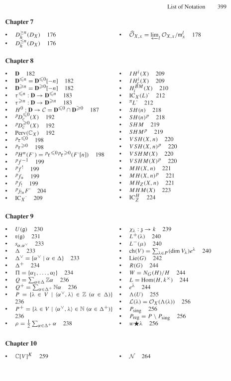
List of Notation 399
Chapter 7
• D≥nh
(DX) 176
• D≤nh
(DX) 176
• OX,x = lim←−lOX,x/ml
x 178
Chapter 8
• D 182• D�n = D�0[−n] 182• D�n = D�0[−n] 182• τ�n : D → D�n 183• τ�n : D → D�n 183• H 0 : D → C = D�0 ∩ D�0 187• pD
�0c (X) 192
• pD�0c (X) 192
• Perv(CX) 192• pτ�0 198• pτ�0 198• pHn(F ·) = pτ�0pτ�0(F ·[n]) 198• pf −1 199• pf ! 199• pf∗ 199• pf! 199• pj!∗F˙ 204• ICX
· 209
• IH i(X) 209• IH i
c (X) 209• HBM
i(X) 210
• ICX(L)˙ 212• πL˙ 212• SH(n) 218• SH(n)p 218• SHM 219• SHMp 219• V SH(X, n) 220• V SH(X, n)p 220• V SHM(X) 220• V SHM(X)p 220• MH(X, n) 221• MH(X, n)p 221• MHZ(X, n) 221• MHM(X) 223• ICH
Z224
Chapter 9
• U(g) 230• r(g) 231• sα,α∨ 233• � 233• �∨ = {α∨ | α ∈ �} 233• �+ 234• $ = {α1, . . . , αl} 234• Q = ∑
α∈� Zα 236• Q+ = ∑
α∈�+ Nα 236• P = {λ ∈ V | 〈α∨, λ〉 ∈ Z (α ∈ �)}
236• P + = {λ ∈ V | 〈α∨, λ〉 ∈ N (α ∈ �+)}
236• ρ = 1
2∑
α∈�+ α 238
• χλ : z → k 239• L+(λ) 240• L−(µ) 240• ch(V ) = ∑
λ∈P (dim Vλ)eλ 240• Lie(G) 242• R(G) 244• W = NG(H)/H 244• L = Hom(H, k×) 244• eλ 244• �(U) 255• L(λ) = OX(�(λ)) 256• Psing 256• Preg = P \ Psing 256• w�λ 256
Chapter 10
• C[V ]K 259 • N 264
400 List of Notation
Chapter 11
• DVY
271
• Dλ = DL(λ+ρ)X
272• Mod(g, χ) 274• Modf (g, χ) 274• Mode
qc(Dλ) 274• Mode
c(Dλ) 274
• Mod(g, K) 284• Mod(g, χ, K) 284• Modf (g, χ, K) 284• Modqc(DY , K) 284• Modc(DY , K) 284• Perv(CY , K) 287
Chapter 12
• ch(M) = ∑µ∈h∗(dim Mµ)eµ 289
• M(λ) = U(g)/(U(g)n
+∑h∈h U(g)(h − λ(h)1)) 290• K(λ) 292• L(λ) = M(λ)/K(λ) 292
• [M(λ) : L(µ)] 294• � = {−wρ − ρ | w ∈ W } 295• K(Modf (g, χ−ρ, B)) 296• H(W) 296• Py,w(q) 296
Chapter 13
• Rn = K(SH(n)p) 311 • R = ⊕n∈Z Rn 311
Appendix A
• k[X] = k[X1, X2, . . . , Xn] 321• V (S) 321• I (W) 321• k[V ] 322• Specm A 322
• D(f ) 323• M 323• OX 325• �X 327• �1
X328
Appendix B
• RnF 332• Sh(T0) 333• C(C) 333• C+(C) 333• C−(C) 333• Cb(C) 333• X˙[k] 334• Mf ˙ 334
• τ�kX· 334• τ�kX· 334• K#(C) (# = ∅, +, −, b) 335• Ab 338• HomFun(A1,A2)(F1, F2) 339
• D#(C) (# = ∅, +, −, b) 342• Q : K#(C) → D#(C) 342• D(C) 342• RF 345• RnF = Hn ◦ RF 347• Hom ˙(•, •) 347• RHomC(•, •) 348• ExtnC(X˙, Y˙) 349• Mod(R) 349• Mod(Rop) 349• (• ⊗R •)˙ 349• • ⊗L
R • 349

List of Notation 401
Appendix C
• Sh(X) 351• F(U) 351• �(U, F ) 351• �c(U, F ) 351• Ab 351• Mod(R) 351• Mod(Rop) 351• Rop 351• Hom(F, G) 351• HomR(M, N) 351• f∗F 352• f!F 352• f −1G 352• F |Z 352• X ×Y Y ′ 352• FZ 352• �Z(X, F ) 352• �Z(F) 352• HomR(M, N) 353• M ⊗R N 354• D#(R) = D#(Mod(R))
(# = ∅, +, −, b) 355
• R�(X, •) 355• R�Z(•) 355• Rf ∗ 355• Rf ! 355• Hi(X, M˙) 356• Hi
Z(X, M˙) 356
• HiZ
(M˙) 356• RHomR(•, •) 357• RHomR(•, •) 357• ExtR(M˙, N˙) 357• ExtR(M˙, N˙) 357• • ⊗L
R • 358
• f !(•) 359• orX/Y 360• orX 360• ωX˙ 360• DX(M˙) 360• Hi
c(X, M˙) 361• M = (Mn, ρn,m) 361• lim←− M 361
Appendix D
• F = {FlA}l∈Z 365• (A, F ) 365• grF A 365• σl 365• supp(M) 370• supp0(M) 370• AnnR(M) 370• 'p(M) 370• SS(M) 371• SS0(M) 371• JM 371
• d(M) 371• mp(M) 371• {a, b} 372• Modf (A) 372
• Dbf
(A) 372
• D = R HomA(•, A) 372• D′ = R HomAop(•, Aop) 372• SS(M ·) 373• j (M) 374• Cs(M) 375
Appendix E
• αX = ∑ni=1 ξidxi 380
• σX = ∑ni=1 dξi ∧ dxi 380
• H : T ∗(T ∗X) � T (T ∗X) 380• Hf 380
• {f, g} 380• C× = C \ {0} 381• ρf : Y ×X T ∗X → T ∗Y 382• �f : Y ×X T ∗X → T ∗X 382

Index
b-function 102D-affine 25F -injective 345F -injective resolution 346F -projective 346G-equivariant 253, 254(g, K)-module 283G-module 242g-module 230K-equivariant D-module 284K-equivariant g-module 283K-equivariant local system 287K-equivariant mixed Hodge module 312K-equivariant perverse sheaf 287l-adic étale cohomology group 217O-lattice 133t-exact 189t-structure 182∂-functor 339
abelian category 333absolutely irreducible 314adjacent 370adjoint group 248adjoint representation 231, 243adjunction formula 80, 357admissible 224affine open covering 29affine variety 325algebraic group 241algebraic meromorphic connection 135,
153algebraic meromorphic extension 136algebraic set 321
algebraic variety 325algebraically constructible sheaf 112annihilating ideal 370Artin–Schreier theorem 294artinian 81associated cycle 60associated fiber bundle 306associated graded module 366associated graded ring 365
base change theorem 48, 54Beilinson–Bernstein 273Beilinson–Bernstein correspondence 298Bernstein filtration 88Borel subalgebra 238Borel subgroup 250Borel–Moore homology group 210Borel–Weil theorem 255bounded 333bounded above 333bounded below 333Bruhat decomposition 252Bruhat ordering 236, 252
canonical 1-form 380canonical sheaf 19Cartan matrix 234Cartan subalgebra 231Cartan’s criterion 231cartesian square 54, 352Cauchy–Kowalevski theorem 106Cauchy–Kowalevski–Kashiwara theorem
105Cech complex 85
404 Index
central character 239, 274character 240, 249, 289characteristic cycle 60, 119characteristic ideal 371characteristic variety 59Chevalley restriction theorem 260cocycle condition 254codimension filtration 375coherent 27, 326coherent continuation representation 310coherent sheaf of rings 27cohomological functor 187, 339cohomological length 50, 163commutative Lie algebra 229comparison theorem 178compatible 204completely reducible 239computational algebraic analysis 62Condition (R) 147conic 59, 381conjugacy class 263connection 18connection matrix 129conormal bundle 64, 381constructibility theorem 113constructible 382constructible sheaf 111convolution product 310coordinate ring 322coroot system 233cotangent bundle 17cotangent sheaf 327, 328Coxeter group 296Coxeter number 261Coxeter transformation 261curve testing criterion 162
de Rham complex 103decomposition theorem 213Deligne theorem 155Deligne’s Riemann–Hilbert correspondence
147, 149Deligne’s theorem 149Deligne–Goresky–MacPherson extension
203derived category 342derived functor 332diagonal embedding 39differential operator 15
dimension 89, 328Dirac delta function 51direct image 21, 40, 352discrete valuation ring 135distinguished triangle 53, 336divisor 139divisor completion 154dominant morphism 137dual 19, 70duality functor 71dualizing complex 111, 360Dynkin diagram 234Dynkin–Kostant theory 265
effictive meromorphic connection (alongdivisors) 142
elementary symmetric polynomial 262enough injectives 331, 354equivariant 284equivariant vector bundle 253étale morphism 123, 329Euler obstruction 119Euler vector field 381exponent 262exterior tensor product 39
filtered A-homomorphism 367filtered D-module 57filtered ring 17, 365finite cohomological dimension 359finite morphism 65finite weak global dimension 358five lemma 107flabby 353flag variety 215, 251flat 354flat connection 18forgetful functor 39formal adjoint 18formal solution 178Fourier transform 87Fréchet space 116Fréchet–Schwartz type 116Frobenius morphism 217Frobenius theorem 104Fuchs 132functor of triangulated categories 339fundamental class 210fundamental solution matrix 130
Index 405
Gabber theorem 62Gabber’s theorem 372GAGA 155GAGA-principle 121Gauss–Manin connection 165generalized Cartan matrix 237generalized Poincaré duality 209geometric Langlands program 215geometric representation theory 213global dimension 369good filtration 58, 366graded module 58graded ring 17, 57graph embedding 55Grauert direct image theorem 143Griffiths transversality 219Gronwall’s inequality 132, 146Grothendieck group 296
Haboush’s theorem 249Hamiltonian isomorphism 379Hamiltonian vector field 380Harish-Chandra homomorphism 239Hartogs theorem 145heart 182Hecke algebra 296highest weight 289highest weight module 289highest weight vector 289Hilbert polynomial 88Hilbert scheme 216Hilbert’s Nullstellensatz 141, 322Hironaka’s desingularization theorem 92Hodge filtration 218Hodge module 221, 311Hodge structure 218holonomic 64holonomic system 64homotopic 335homotopic to 0 335homotopy category 335homotopy equivalence 335horizontal section 104, 128, 140hyperextension group 349hypergeometric function 62hypertorsion group 349
injective resolution 331injective sheaf 354
integrability condition 18integrable connection 18, 61intersection cohomology complex 178,
202, 209, 224intersection cohomology group 202, 209invariant distribution 215invariant polynomial 259invariant polynomial ring 259inverse image 21, 33, 352involutive 62, 372, 379irreducible 233irreducible representation 239irregularity sheaf 173isotropic 379Iwahori–Hecke algebra 296
Jacobson–Morozov theorem 265Jantzen’s deformation argument 299Jordan decomposition 243, 263Jordan–Hölder series 95
Kac–Moody Lie algebra 237Kashiwara
conjecture on semisimple holonomicsystems 299
constructibility theorem 113equivalence 48local index theorem 119
Kazhdan–Lusztig conjecture 297Kazhdan–Lusztig polynomials 297Killing form 231Koszul complex 152Koszul resolution 35
Lagrangian 212, 379Langlands classification 287left derived functor 345left D-module 17left t-exact 189Leibniz rule 16length 370Lie algebra 229, 242Lie bracket 229Lie derivative 19linear algebraic group 241local coordinate system 15, 329local Euler–Poincaré index 118local system 104localization 340localization functor 342
406 Index
localization of category 340logarithmic pole 144longest element 236
mapping cone 334maximal torus 244maximally overdetermined system 64meromorphic connection 128, 139micro-support 109, 212microdifferential operator 109microlocal Riemann–Hilbert correspondence
178microlocalization 178middle perversity 191minimal extension 95, 178, 203, 204Mittag-Leffler condition 361mixed Hodge structure 219mixed weight 224moderate growth 130moment map 270monodromy matrix 130monodromy representation 146morphism of Hodge structures 218morphism of triangles 336multiplicative system 340multiplicity 60, 89, 119, 294Mumford’s conjecture 249
Nagata counterexample to Hilbert’s 14thproblem 259
Nakayama lemma 27natural transformation 339nilpotent cone 264, 270nilpotent conjugacy class 263nilpotent part 263non-characteristic 65non-characteristic deformation lemma
361, 363normal crossing 143normalization 214
octahedral axiom 337Oda’s rule 20ODE 127opposite category 348order filtration 16ordinary differential equation 18, 127Ore condition 340orientation sheaf 360
PBW 230perverse cohomology 198perverse sheaf 113, 114, 198perverse t-structure 191Poincaré duality 202Poincaré lemma 105Poincaré–Verdier duality 359Poincaré–Birkhoff–Witt theorem 230Poisson bracket 372, 380polarizable 218, 219polarization of Hodge structures 218prevariety 325principal ideal domain 135principal open subset 323principal symbol 17projection formula 56, 359projective system 361proper direct image 352pure weight 224
quasi-coherent 326quasi-coherent sheaf 25quasi-compact 325quasi-inverse 21quasi-isomorphism 332, 333quasi-projective 30
radical 231, 244, 322radical ideal 323Radon transform 48rationally smooth 211reduced 322reductive 244reflexive 141regular 133, 135–137, 153, 161, 162regular conjugacy class 267regular element 267regular extension (of analytic integrable
connections) 147regular function 325regular holonomic D-module 161regular meromorphic connection (along
divisors) 141regular ring 372regular singularity 136relative de Rham complex 45relative orientation sheaf 360relevant 215, 216representation 230, 242

Index 407
residue 144resolution of singularities 269Riemann–Hilbert correspondence 174right derivable 345right derived functor 345right D-module 19right localizable 344right localization 344right t-exact 189root datum 245root lattice 236root system 232, 233, 245
Sato’s hyperfunction 116Schubert cell 252Schubert variety 252Schwartz distribution 77, 178semisimple 231, 244semisimple conjugacy class 263semisimple element 243semisimple part 263semismall 213separated 325Serre’s twisted sheaf 256shifted complex 334shifted inverse image 33side-changing 21simple 231simple holonomic D-module 95simple root 234singular support 59, 371small 213smooth 328smooth completion 92solution complex 103solvable Lie algebra 231Spencer resolution 44Springer representation 216Springer resolution 270stack 198standard t-structure 182stratification 111, 382stratum 111, 382strict 218, 367strict support 221
structure sheaf 15, 325support (of perverse sheaves) 198symplectic form 379, 380symplectic manifold 380symplectic vector space 379
tangent sheaf 15, 327Tate twist 221theory of invariant polynomials 259theory of weights 224thick subcategory 343total multiplicity 82total symbol 16trace map 77transfer bimodules 23triangle 336triangulated category 339truncated complex 334twisted differential operator 272twisted intersection cohomology complex
212twisted inverse image 359
underlying real manifold 108unipotent element 243
variation of Hodge structures 219Verdier dual 111, 360Verma module 291
weight 218, 239weight lattice 236weight space 239Weil conjecture 217Weyl algebra 86Weyl group 234Weyl vector 238Weyl’s character formula 240Weyl’s denominator formula 241Whitney condition 383Whitney stratification 114, 383Whitney’s umbrella 384
Zariski topology 321zero-section 60Zorn’s lemma 363

Progress in MathematicsEdited by:
Hyman Bass Joseph OesterléDept. of Mathematics Equipe de théorie des nombresUniversity of Michigan Université Paris 6Ann Arbor, MI 48109 175 rue du ChevaleretUSA 75013 Paris, [email protected] [email protected]
Progress in Mathematics is a series of books intended for professional mathematicians and scientists,encompassing all areas of pure mathematics. This distinguished series, which began in 1979, includesauthored monographs and edited collections of papers on important research developments as well asexpositions of particular subject areas.
We encourage preparation of manuscripts in some form of T X for delivery in camera-ready copywhich leads to rapid publication, or in electronic form for interfacing with laser printers or typesetters.
Proposals should be sent directly to the editors or to: Birkhäuser Boston, 675 Massachusetts Avenue,Cambridge, MA 02139, USA or to Birkhauser Verlag, 40-44 Viadukstrasse, CH-4051 Basel,Switzerland.
161 SAGAN/STANLEY (eds). Mathematical Essays in Honor of Gian-Carlo Rota162 ARNOLD/GREUEL/STEENBRINK. Singularities: The Brieskorn Anniversary Volume163 BERNDT/SCHMIDT. Elements of the Representaiton Theory of the Jacobi Group164 ROUSSARIE. Bifurcations of Planar Vector Fields and Hilbert's Sixteenth Problem165 MIGLIORE. Introduction to Liaison Theory and Deficiency Modules166 ELIAS/GIRAL/MIRO-ROIG/ZARZUELA (eds). Six Lectures on Commutative Algebra167 FACCHINI. Module Theory168 BALOG/KATONA/SZA'SZ/RECSKI (eds). European Congress of Mathematics, Budapest, July 22-26, 1996. Vol. I169 BALOG/KATONA/SZA'SZ/RECSKI (eds). European Congress of Mathematics, Budapest, July 22-26, 1996. Vol. II168/169 Sets Vols I, II170 PATERSON. Groupoids, Inverse Semigroups, and their Operator Algebras171 REZNIKOV/SCHAPPACHER (eds). Regulators in Analysis, Geometry and Number Theory172 BRYLINSKI/BRYLINSKI/NISTOR/TSYGAN/ XU (eds). Advances in Geometry
E
150 SHIOTA. Geometry of Subanalytic and Semialgebraic Sets151 HUMMEL. Gromov's Compactness Theorem for Pseudo-holomorphic Curves152 GROMOV. Metric Structures for Riemannian and Non-Riemannian Spaces. Sean Bates (translator)153 BUESCU. Exotic Attractors: From Liapunov Stability to Riddled Basins154 BÖTTCHER/KARLOVICH. Carleson Curves, Muckenhoupt Weights, and Toeplitz Operators155 DRAGOMIR/ORNEA. Locally Conformal
Kähler Geometry156 GUIVARC'H/JI/TAYLOR. Compactifications of Symmetric Spaces157 MURTY/MURTY. Non-vanishing of L-functions and Applications158 TIRAO/VOGAN/WOLF (eds). Geometry and Representation Theory of Real and p-adic Groups159 THANGAVELU. Harmonic Analysis on the Heisenberg Group160 KASHIWARA/MATSUO/SAITO/SATAKE (eds). Topological Field Theory, Primitive Forms and Related Topics
Alan WeinsteinDept. of MathematicsUniversity of CaliforniaBerkeley, CA [email protected]
173 DRÄXLER/MICHLER/RINGEL (eds). Compu tational Methods for Representation of Groups and Algebras: Euroconference in Essen174 GOERSS/JARDINE. Simplicial Homotopy Theory175 BAÑUELOS/MOORE. Probabilistic Behavior of Harmonic Functions176 BASS/LUBOTZKY. Tree Lattices177 BIRKENHAKE/LANGE. Complex Tori178 PUIG. On the Local Structure of Morita and Rickard Equivalence Between Brauer Blocks179 MORALES RUIZ. Differential Galois Theory and Non-Integrability of Hamiltonian Systems180 PATERNAIN. Geodesic Flows181 HAUSER/LIPMAN/OORT/QUIRÓS (eds).
Resolution of Singularities: In Tribute to Oscar Zariski182 BILLEY/LAKSHMIBAI. Singular Loci of Schubert Varieties183 KAPOVICH. Hyperbolic Manifolds and Discrete Groups184 du SAUTOY/SEGAL/SHALEV (eds). New Horizons in pro-p Groups185 FARAUT/KANEYUKI/KORÁNYI/LU/ROOS. Analysis and Geometry on Complex Homogeneous Domains186 KLEINERT. Units in Skew Fields187 BOST/LOESER/RAYNAUD. Courbes Semi-stables et Groupe Fondamental en Géométrie Algébrique188 DOLBEAULT/IORDAN/HENKIN/SKODA/ TRÉPREAU (eds). Complex Analysis and Geometry: International Conference in Honor of Pierre Lelong189 ANDRÉ/BALDASSARI. DeRham Coho- mology of Differential Modules on Algebraic Varieties190 van den ESSEN. Polynomial Automor- phisms and the Jacobian Conjecture.191 KASHIWARA/MIWA (eds). Physical Combinatorics192 DEHORNOY. Braids and Self-Distributivity193 KNUDSON. Homology of Linear Groups194 JUHL. Cohomological Theory of Dynamical Zeta Functions195 FABER/van der GEER/OORT (eds). Moduli of Abelian Varieties
196 AGUADÉ/BROTO/CASACUBERTA (eds). Cohomological Methods in Homotopy Theory197 CHERIX/COWLING/JOLISSAINT/JULG/
VALETTE (eds). Groups with the Haagerup property198 LANDSMAN/PFLAUM/SCHLICHENMAIER
(eds). Quantization of Singular Symplectic Quotients199 PEYRE/TSCHINKEL. Rational Points on Algebraic Varieties200 GOLUBITSKY/STEWART. The Symmetry Perspective201 CASACUBERTA/MIRÓ-ROIG/VERDERA/
XAMBÓ-DESCAMPS (eds). European Congress of Mathematics, Volume 1202 CASACUBERTA/MIRÓ-ROIG/VERDERA/
XAMBÓ-DESCAMPS (eds). European Congress of Mathematics, Volume 2203 BLAIR. Riemannian Geometry of Contact and Symplectic Manifolds204 KUMAR. Kac–Moody Groups, their Flag Varieties, and Representation Theory205 BOUWKNEGT/WU. Geometric Analysis and Applications to Quantum Field Theory206 SNAITH. Algebraic K-groups as Galois Modules207 LONG. Index Theory for Symplectic Paths with Applications208 TURAEV. Torsions of 3-dimensional Manifolds209 UNTERBERGER. Automorphic Pseudo- differential Analysis and Higher Level Weyl Calculi210 JOSEPH/MELNIKOV/RENTSCHLER (eds). Studies in Memory of Issai Schur211 HERNÁNDEZ-LERMA/LASSERE. Markov Chains and Invariant Probabilities212 LUBOTZKY/SEGAL. Subgroup Growth213 DUVAL/GUIEU/OVSIENKO (eds). The Orbit Method in Geometry and Physics. In Honor of A.A. Kirillov214 DUNGEY/TER ELST/ROBINSON. Analysis on Lie Groups with Polynomial Growth215 ARONE/HUBBUCK/LEVI/WEISS. Algebraic Topology.216 BOROVIK/GELFAND/WHITE. Coxeter Matroids.217 THANGAVELU. An Introduction to the Uncertainty Principle: Hardy's Theorem on Lie Groups.

218 FRESNEL/VAN DER PUT. Rigid Analytic Geometry and Its Applications.219 SURIS. The Problem of Integrable Discretization: Hamiltonian Approach220 DELORME/VERGNE (eds). Noncommutative Harmonic Analysis: In Honor of Jacques Carmona221 Gray. Tubes, 2nd Edition222 Ortega/Ratiu. Momentum Maps and Hamiltonian Reduction223 Andreu-Vaillo/Caselles/Mazón. Parabolic Quasilinear Equations Minimizing Linear Growth Functionals224 Cremona/Lario/Quer/Ribet (eds). Modular Curves and Abelian Varieties225 Andersson/Passare/Sigurdsson. Complex Convexity and Analytic Functionals226 Poonen/Tschinkel (eds). Arithmetic of Higher-Dimensional Algebraic Varieties227 Lepowsky/Li. Introduction to Vertex Operator Algebras and Their Representations228 Anker/Orsted (eds). Lie Theory: Lie Algebras and Representations229 Anker/Orsted (eds). Lie Theory: Unitary Representations and Compactifications of Symmetric Spaces230 Anker/Orsted (eds). Lie Theory: Harmonic Analysis on Symmetric Spaces—General Plancheral Theorems231 Brion/Kumar. Frobenius Splitting Methods in Geometry and Representation Theory232 Marsden/Ratiu (eds). The Breadth of Symplectic and Poisson Geometry: Festschrift in Honor of Alan Weinstein233 David. Singular Sets of Minimizers for the Mumford–Shah Functional234 Kowalski/Musso/Perrone (eds). Complex, Contact and Symmetric Manifolds: In Honor of L. Vanhecke235 Bogomolov/Tschinkel (eds). Geometric Methods in Algebra and Number Theory236 Hotta/Takeuchi/Tanisaki. D-Modules, Perverse Sheaves, and Representation Theory237 Kulish/Manojlovic/Samtleben (eds). Infinite Dimensional Algebras and Quantum Integrable Systems238 Sabadini/Struppa/Walnut (eds). Harmonic Analysis, Signal Processing, and Complexity: Festschrift in Honor of the 60th Birthday of Carlos A. Berenstein
239 van der Geer/Moonen/Schoof (eds). Number Fields and Function Fields — Two Parallel Worlds240 Ambrosetti/Malchiodi. Perturbation Methods and Semilinear Elliptic Problems on Rn
241 Seade. On the Topology of Isolated Singularities in Analytic Spaces242 Dufour/Zung. Poisson Structures and their Normal Forms243 Bernstein/Hinich/Melnikov (eds). Studies in Lie Theory: In honor of A. Joseph244 Etingof/Retakh/Singer (eds). The Unity of Mathematics: In Honor of Ninetieth Birthday of I.M. Gelfand245 Fels/Huckleberry/Wolf. Cycle Spaces of Flag Domains: A Complex Geometric View246 Dragomir/Tomassini. Differential Geometry and Analysis on CR Manifolds247 Baves. The Algebra of Secondary Cohomology Operations.248 Bartholdi et al. (eds). Infinite Groups: Geometric, Combinatorial and Dynamical Aspects249 Kock/Vainsencher. An Invitation to Quantum Cohomology: Kontsevich's Formula for Rational Plane Curves250 Unterberger. The Fourfold Way in Real Analysis and an Alternative to the Metaplectic251 Boutet de Monvel/Buchholz/ Iagolnitzer/Moschella. Rigorous Quantum Field Theory: A Festschrift for Jacques Bros252 Maeda/Michor/Ochiai/Yoshioka. From Geometry to Quantum Mechanics: In Honor of Hideki Omori253 Ginzburg. Algebraic Geometry and Number Theory: In Honor of Vladimir Drinfeld's 50th Birthday254 Ma/Marinescu. Holomorphic Morse Inequalities and Bergman Kernels255 Kobayashi/Toshiyuki/Schmid/Yang. Representation Theory and Automorphic Forms.256 Borthwick. Spectral Theory of Infinite-Area Hyperbolic Surfaces.257 Lakshmibai/Littelmann. Schubert Varieties.258 Gan/Kudla/Tschinkel. Eisenstein Series and Applications.259 Capogna/Danielli. An Introduction to the Heisenberg Group and the Sub-Rieman nian Isoperimetric Problem.
260 Holzapfel/Uludag/Yoshida. Arithmetic and Geometry Around Hypergeometric Functions.261 Stout. Polynomial Convexity
ˇ

![Abdul-Awal, S. M., Hotta, C. T., Davey, M. P., Dodd, A. …Abdul-Awal, S. M., Hotta, C. T., Davey, M. P., Dodd, A. N., Smith, A. G., & Webb, A. A. R. (2016). NO-mediated [Ca2+]cyt](https://img.pdfslide.us/doc/110x75/5fcfbc114da5980a514b1821/abdul-awal-s-m-hotta-c-t-davey-m-p-dodd-a-abdul-awal-s-m-hotta.jpg)