Progress in Applied CFD – CFD2017

2Proceedings of the 12th International Conference on Computational Fluid Dynamics in the Oil & Gas, Metallurgical and Process Industries

SINTEFPROCEEDINGS

Progress in Applied CFD –CFD2017

Editors: Jan Erik Olsen and Stein Tore Johansen

Progress in Applied CFD – CFD2017

Proceedings of the 12th International Conference on Computational Fluid Dynamics

in the Oil & Gas, Metallurgical and Process Industries

SINTEF Proceedings

SINTEF Academic Press

SINTEF Proceedings no 2 Editors: Jan Erik Olsen and Stein Tore JohansenProgress in Applied CFD – CFD2017

Selected papers from 10th International Conference on Computational Fluid Dynamics in the Oil & Gas, Metal lurgical and Process Industries

Key words:CFD, Flow, Modelling

Cover, illustration: Arun Kamath

ISSN 2387-4295 (online)ISBN 978-82-536-1544-8 (pdf)

© Copyright SINTEF Academic Press 2017The material in this publication is covered by the provisions of the Norwegian Copyright Act. Without any special agreement with SINTEF Academic Press, any copying and making available of the material is only allowed to the extent that this is permitted by law or allowed through an agreement with Kopinor, the Reproduction Rights Organisation for Norway. Any use contrary to legislation or an agreement may lead to a liability for damages and confiscation, and may be punished by fines or imprisonment

SINTEF Academic PressAddress: Forskningsveien 3 B PO Box 124 Blindern N-0314 OSLOTel: +47 73 59 30 00Fax: +47 22 96 55 08

www.sintef.no/byggforskwww.sintefbok.no

SINTEF ProceedingsSINTEF Proceedings is a serial publication for peer-reviewed conference proceedings on a variety of scientific topics.The processes of peer-reviewing of papers published in SINTEF Proceedings are administered by the conference organizers and proceedings editors. Detailed procedures will vary according to custom and practice in each scientific community.

PREFACE

This book contains all manuscripts approved by the reviewers and the organizing committee of the

12th International Conference on Computational Fluid Dynamics in the Oil & Gas, Metallurgical and

Process Industries. The conference was hosted by SINTEF in Trondheim in May/June 2017 and is also

known as CFD2017 for short. The conference series was initiated by CSIRO and Phil Schwarz in 1997.

So far the conference has been alternating between CSIRO in Melbourne and SINTEF in Trondheim.

The conferences focuses on the application of CFD in the oil and gas industries, metal production,

mineral processing, power generation, chemicals and other process industries. In addition pragmatic

modelling concepts and bio‐mechanical applications have become an important part of the

conference. The papers in this book demonstrate the current progress in applied CFD.

The conference papers undergo a review process involving two experts. Only papers accepted by the

reviewers are included in the proceedings. 108 contributions were presented at the conference

together with six keynote presentations. A majority of these contributions are presented by their

manuscript in this collection (a few were granted to present without an accompanying manuscript).

The organizing committee would like to thank everyone who has helped with review of manuscripts,

all those who helped to promote the conference and all authors who have submitted scientific

contributions. We are also grateful for the support from the conference sponsors: ANSYS, SFI Metal

Production and NanoSim.

Stein Tore Johansen & Jan Erik Olsen

3

Organizing committee:

Conference chairman: Prof. Stein Tore Johansen

Conference coordinator: Dr. Jan Erik Olsen

Dr. Bernhard Müller

Dr.Sigrid Karstad Dahl

Dr.Shahriar Amini

Dr.Ernst Meese

Dr.Josip Zoric

Dr.Jannike Solsvik

Dr.Peter Witt

Scientific committee:

Stein Tore Johansen, SINTEF/NTNU

Bernhard Müller, NTNU

Phil Schwarz, CSIRO

Akio Tomiyama, Kobe University

Hans Kuipers, Eindhoven University of Technology

Jinghai Li, Chinese Academy of Science

Markus Braun, Ansys

Simon Lo, CD‐adapco

Patrick Segers, Universiteit Gent

Jiyuan Tu, RMIT

Jos Derksen, University of Aberdeen

Dmitry Eskin, Schlumberger‐Doll Research

Pär Jönsson, KTH

Stefan Pirker, Johannes Kepler University

Josip Zoric, SINTEF

4

CONTENTS

PRAGMATIC MODELLING ................................................................................................................ 9 On pragmatism in industrial modeling. Part III: Application to operational drilling ............................. 11 CFD modeling of dynamic emulsion stability ........................................................................................ 23 Modelling of interaction between turbines and terrain wakes using pragmatic approach ................. 29 FLUIDIZED BED .............................................................................................................................. 37 Simulation of chemical looping combustion process in a double looping fluidized bed reactor with cu‐based oxygen carriers .................................................................................................. 39 Extremely fast simulations of heat transfer in fluidized beds ............................................................... 47 Mass transfer phenomena in fluidized beds with horizontally immersed membranes ....................... 53 A Two‐Fluid model study of hydrogen production via water gas shift in fluidized bed membrane reactors .............................................................................................................................. 63 Effect of lift force on dense gas‐fluidized beds of non‐spherical particles ........................................... 71 Experimental and numerical investigation of a bubbling dense gas‐solid fluidized bed ...................... 81 Direct numerical simulation of the effective drag in gas‐liquid‐solid systems ..................................... 89 A Lagrangian‐Eulerian hybrid model for the simulation of direct reduction of iron ore in fluidized beds..................................................................................................................................... 97 High temperature fluidization ‐ influence of inter‐particle forces on fluidization behavior .............. 107 Verification of filtered two fluid models for reactive gas‐solid flows ................................................. 115 BIOMECHANICS ........................................................................................................................... 123 A computational framework involving CFD and data mining tools for analyzing disease in cartoid artery ...................................................................................................................................... 125 Investigating the numerical parameter space for a stenosed patient‐specific internal carotid artery model ............................................................................................................................ 133 Velocity profiles in a 2D model of the left ventricular outflow tract, pathological case study using PIV and CFD modeling .............................................................................................. 139 Oscillatory flow and mass transport in a coronary artery ................................................................... 147 Patient specific numerical simulation of flow in the human upper airways for assessing the effect of nasal surgery ................................................................................................................... 153 CFD simulations of turbulent flow in the human upper airways ........................................................ 163 OIL & GAS APPLICATIONS ............................................................................................................ 169 Estimation of flow rates and parameters in two‐phase stratified and slug flow by an ensemble Kalman filter ....................................................................................................................... 171 Direct numerical simulation of proppant transport in a narrow channel for hydraulic fracturing application .......................................................................................................................... 179 Multiphase direct numerical simulations (DNS) of oil‐water flows through homogeneous porous rocks ................................................................................................................ 185 CFD erosion modelling of blind tees ................................................................................................... 191 Shape factors inclusion in a one‐dimensional, transient two‐fluid model for stratified and slug flow simulations in pipes ...................................................................................................... 201 Gas‐liquid two‐phase flow behavior in terrain‐inclined pipelines for wet natural gas transportation ............................................................................................................................... 207

NUMERICS, METHODS & CODE DEVELOPMENT ........................................................................... 213 Innovative computing for industrially‐relevant multiphase flows ...................................................... 215 Development of GPU parallel multiphase flow solver for turbulent slurry flows in cyclone .............. 223 Immersed boundary method for the compressible Navier–Stokes equations using high order summation‐by‐parts difference operators ........................................................................ 233 Direct numerical simulation of coupled heat and mass transfer in fluid‐solid systems ..................... 243 A simulation concept for generic simulation of multi‐material flow, using staggered Cartesian grids ........................................................................................................... 253 A cartesian cut‐cell method, based on formal volume averaging of mass, momentum equations ......................................................................................................................... 265 SOFT: a framework for semantic interoperability of scientific software ............................................ 273 POPULATION BALANCE ............................................................................................................... 279 Combined multifluid‐population balance method for polydisperse multiphase flows ...................... 281 A multifluid‐PBE model for a slurry bubble column with bubble size dependent velocity, weight fractions and temperature ........................................................................................ 285 CFD simulation of the droplet size distribution of liquid‐liquid emulsions in stirred tank reactors ........................................................................................................................ 295 Towards a CFD model for boiling flows: validation of QMOM predictions with TOPFLOW experiments ....................................................................................................................... 301 Numerical simulations of turbulent liquid‐liquid dispersions with quadrature‐based moment methods ................................................................................................................................ 309 Simulation of dispersion of immiscible fluids in a turbulent couette flow ......................................... 317 Simulation of gas‐liquid flows in separators ‐ a Lagrangian approach ................................................ 325 CFD modelling to predict mass transfer in pulsed sieve plate extraction columns ............................ 335 BREAKUP & COALESCENCE .......................................................................................................... 343 Experimental and numerical study on single droplet breakage in turbulent flow ............................. 345 Improved collision modelling for liquid metal droplets in a copper slag cleaning process ................ 355 Modelling of bubble dynamics in slag during its hot stage engineering ............................................. 365 Controlled coalescence with local front reconstruction method ....................................................... 373 BUBBLY FLOWS ........................................................................................................................... 381 Modelling of fluid dynamics, mass transfer and chemical reaction in bubbly flows .......................... 383 Stochastic DSMC model for large scale dense bubbly flows ............................................................... 391 On the surfacing mechanism of bubble plumes from subsea gas release .......................................... 399 Bubble generated turbulence in two fluid simulation of bubbly flow ................................................ 405 HEAT TRANSFER .......................................................................................................................... 413 CFD‐simulation of boiling in a heated pipe including flow pattern transitions using a multi‐field concept .................................................................................................................. 415 The pear‐shaped fate of an ice melting front ..................................................................................... 423 Flow dynamics studies for flexible operation of continuous casters (flow flex cc) ............................. 431 An Euler‐Euler model for gas‐liquid flows in a coil wound heat exchanger ........................................ 441 NON‐NEWTONIAN FLOWS ........................................................................................................... 449 Viscoelastic flow simulations in disordered porous media ................................................................. 451 Tire rubber extrudate swell simulation and verification with experiments ....................................... 459 Front‐tracking simulations of bubbles rising in non‐Newtonian fluids ............................................... 469 A 2D sediment bed morphodynamics model for turbulent, non‐Newtonian, particle‐loaded flows ........................................................................................................................... 479

METALLURGICAL APPLICATIONS .................................................................................................. 491 Experimental modelling of metallurgical processes ........................................................................... 493 State of the art: macroscopic modelling approaches for the description of multiphysics phenomena within the electroslag remelting process ....................................................................... 499 LES‐VOF simulation of turbulent interfacial flow in the continuous casting mold ............................. 507 CFD‐DEM modelling of blast furnace tapping ..................................................................................... 515 Multiphase flow modelling of furnace tapholes ................................................................................. 521 Numerical predictions of the shape and size of the raceway zone in a blast furnace ........................ 531 Modelling and measurements in the aluminium industry ‐ Where are the obstacles? ..................... 541 Modelling of chemical reactions in metallurgical processes ............................................................... 549 Using CFD analysis to optimise top submerged lance furnace geometries ........................................ 555 Numerical analysis of the temperature distribution in a martensic stainless steel strip during hardening ......................................................................................................................... 565 Validation of a rapid slag viscosity measurement by CFD ................................................................... 575 Solidification modeling with user defined function in ANSYS Fluent .................................................. 583 Cleaning of polycyclic aromatic hydrocarbons (PAH) obtained from ferroalloys plant ...................... 587 Granular flow described by fictitious fluids: a suitable methodology for process simulations .......... 593 A multiscale numerical approach of the dripping slag in the coke bed zone of a pilot scale Si‐Mn furnace ..................................................................................................................... 599 INDUSTRIAL APPLICATIONS ......................................................................................................... 605 Use of CFD as a design tool for a phospheric acid plant cooling pond ............................................... 607 Numerical evaluation of co‐firing solid recovered fuel with petroleum coke in a cement rotary kiln: Influence of fuel moisture ................................................................................... 613 Experimental and CFD investigation of fractal distributor on a novel plate and frame ion‐exchanger ........................................................................................................................... 621 COMBUSTION ............................................................................................................................. 631 CFD modeling of a commercial‐size circle‐draft biomass gasifier ....................................................... 633 Numerical study of coal particle gasification up to Reynolds numbers of 1000 ................................. 641 Modelling combustion of pulverized coal and alternative carbon materials in the blast furnace raceway ......................................................................................................................... 647 Combustion chamber scaling for energy recovery from furnace process gas: waste to value ..................................................................................................................................... 657 PACKED BED ................................................................................................................................ 665 Comparison of particle‐resolved direct numerical simulation and 1D modelling of catalytic reactions in a packed bed ................................................................................................. 667 Numerical investigation of particle types influence on packed bed adsorber behaviour .................. 675 CFD based study of dense medium drum separation processes ........................................................ 683 A multi‐domain 1D particle‐reactor model for packed bed reactor applications ............................... 689 SPECIES TRANSPORT & INTERFACES ............................................................................................ 699 Modelling and numerical simulation of surface active species transport ‐ reaction in welding processes ........................................................................................................... 701 Multiscale approach to fully resolved boundary layers using adaptive grids ..................................... 709 Implementation, demonstration and validation of a user‐defined wall function for direct precipitation fouling in Ansys Fluent ................................................................................... 717

FREE SURFACE FLOW & WAVES ................................................................................................... 727 Unresolved CFD‐DEM in environmental engineering: submarine slope stability and other applications................................................................................................................................ 729 Influence of the upstream cylinder and wave breaking point on the breaking wave forces on the downstream cylinder .................................................................................................... 735 Recent developments for the computation of the necessary submergence of pump intakes with free surfaces ................................................................................................................... 743 Parallel multiphase flow software for solving the Navier‐Stokes equations ...................................... 752 PARTICLE METHODS .................................................................................................................... 759 A numerical approach to model aggregate restructuring in shear flow using DEM in Lattice‐Boltzmann simulations ............................................................................................................ 761 Adaptive coarse‐graining for large‐scale DEM simulations ................................................................. 773 Novel efficient hybrid‐DEM collision integration scheme ................................................................... 779 Implementing the kinetic theory of granular flows into the Lagrangian dense discrete phase model ................................................................................................................ 785 Importance of the different fluid forces on particle dispersion in fluid phase resonance mixers ................................................................................................................................ 791 Large scale modelling of bubble formation and growth in a supersaturated liquid ........................... 798 FUNDAMENTAL FLUID DYNAMICS ............................................................................................... 807 Flow past a yawed cylinder of finite length using a fictitious domain method .................................. 809 A numerical evaluation of the effect of the electro‐magnetic force on bubble flow in aluminium smelting process ............................................................................................................ 819 A DNS study of droplet spreading and penetration on a porous medium .......................................... 825 From linear to nonlinear: Transient growth in confined magnetohydrodynamic flows ..................... 831

A 2D SEDIMENT BED MORPHODYNAMICS MODEL FOR TURBULENT, NON-NEWTONIAN, PARTICLE-LOADED FLOWS

Alexander BUSCH1*, Milad KHATIBI2, Stein T. JOHANSEN1,3, Rune W. TIME2 1 Norwegian University of Science and Technology (NTNU), Trondheim, NORWAY

2 University of Stavanger (UiS), Stavanger, NORWAY 3 SINTEF Materials and Chemistry, Trondheim, NORWAY

* E-mail: [email protected]

ABSTRACT In petroleum drilling, cuttings transport problems, i.e. an accumulation of drilled of solids in the wellbore, are a major contributor to well downtime and have therefore been extensively researched over the years, both experimentally and through simulation. In recent years, Computational Fluid Dynamics (CFD) has been used intensively due to increasing available computational power. Here, the problem of cuttings transport is typically investigated as a laminar/turbulent, potentially non-Newtonian (purely shear-thinning) multiphase problem. Typically, an Eulerian-Eulerian two-fluid model concept is utilized, where the particle phase is treated as a second continuous phase. Optionally, a granular flow model, based on the Kinetic Theory of Granular Flow (KTGF), may be used to account for the dense granular flow properties of cuttings forming a sediment bed. One issue of the state of the art CFD approach as described above is the proper resolution of the bed interface, as this may not be accurately resolved in an industrial-relevant CFD simulation. In this paper, an alternative approach is taken based on modeling concepts used in environmental sediment transport research (rivers, deserts). Instead of including the sediment bed in the computational domain, the latter is limited to the part of the domain filled with the particle-loaded continuous fluid phase. Consequently, the bed interface becomes a deformable domain boundary, which is updated based on the solution of an additional scalar transport equation for the bed height, which is based on the so-called Exner equation (Exner, 1925), a mass conservation equation accounting for convection, and additionally deposition and erosion in the bed load layer. These convective fluxes are modeled with closures relating these fluxes to flow quantities. As a first step, a 2D model was implemented in ANSYS Fluent R17.2 using Fluent’s dynamic mesh capabilities and User-Defined Function (UDF) interfaces. The model accounts for local bed slope, hindered settling, and non-Newtonian, shear-thinning viscosity of the fluid phase as well as turbulence. Model results are benchmarked with experimental data for five different operating points. Most probably due to the utilized unsteady Reynolds-Averaging framework (URANS), the model is not capable of predicting flow-induced dunes; however, it does predict bed deformation as a consequence of for instance non-equilibrium boundary conditions. Other model issues such as e.g. non-Newtonian formulations of the closures are identified and discussed.

Keywords: Drilling, cuttings transport, particle transport, sediment transport, bed load, turbulence, non-Newtonian, multiphase, deforming mesh, CFD.

NOMENCLATURE

Greek Symbols α Volume fraction, [-]. β Local bed slope, [rad].

�̇�𝛾 Shear rate, mag. of deformation rate tensor, [1/s]. ρ Mass density, [kg/m3]. µ Dynamic viscosity, [kg/m.s]. ν Kinematic viscosity, [kg/m.s]. τ (Wall) Shear stress, [Pa]. ϕ Angle of repose, [rad]. θ Non-dimensional shear stress, Shields number, [-]. ω Specific dissipation rate [1/s].

Latin Symbols c Coefficient of drag, [-]. C Bed slope model constant, ≈ 1.5, [-]. d Diameter, [m]. D Deposition, [m/s]. D Rate of deformation tensor, [m/s²]. E Entrainment, [m/s]. F Momentum exchange term, [kg/s².m³]. g Gravitational acceleration, [m/s²]. h Bed height, [m]. k Turbulent kinetic energy, [m²/s²]. n Exp. in rheo. models & hind. settling function, [-]. q Vol. bed load transport rate per unit width, [m³/s.m]. s Ratio of solid and fluid densities, [-]. S Source term, [kg/s.m³]. t Time, [s]. T Stress tensor, [kg.m/s².m³]. u Velocity vector, [m/s]. v Vertical velocity component, [m/s]. V Volume, [m³].

Sub/superscripts 0 Horizontal or initial or zero. * Non-dimensional. b Bed. cr Critical/Treshold. CR Cross. D Drag. f Fluid. i Phase index. PL Power-law. s Solid. t Turbulent. T Transposed. x x-direction in space. y y-direction in space. z z-direction in space.

Abbreviations 2D Two-dimensional in space. 3D Three-dimensional in space. CFD Computational Fluid Dynamics.

479

mailto:[email protected]?subject=CFD2017%20-%20Bed%20morphodynamics%20paper

GNF Generalized Newtonian Fluid. H2O Water. KTGF Kinetic theory of granular flow. PAC Polyannionic cellulose. OBM Oil-based muds. UDF User-Defined Function. URANS Unsteady Reynolds-Averaged-Navier-Stokes. SST Shear Stress Transport. VLES Very Large-Eddy Simulation. WBM Water-based muds.

INTRODUCTION

Existing research body and praxis Cuttings transport in wellbores, herein termed wellbore flows, is a multiscale problem, both in space and time but also regarding the different levels of physical complexity. In general, wellbore flows incorporate non-Newtonian rheology, dispersed and potentially dense packed solids (cuttings forming a sediment bed) and the flow may be turbulent. The domain of interest is an annulus, formed by the drill pipe, which may also rotate, inside the wellbore. Conceptually, the flow may be categorized into three layers: (1) A flowing mixture layer, where particles are transported in a heterogeneous suspension. (2) An intermediate layer, where particles roll and slide on top of each other, which is just a few particle diameters thick. (3) Depending on the various parameters involved, a densely packed, and in most cases stationary, cuttings bed may form at the lower part of the annulus. Several scientists, e.g. Doron and Barnea (1993); Savage et al. (1996) or more recently Bello et al. (2011); Nossair et al. (2012); Goharzadeh et al. (2013); Corredor et al. (2016), have experimentally investigated wellbore flows in laboratory flow loops. Corredor et al. (2016) determined the critical velocities for the initiation of particle movement with rolling, saltation, and suspension. They found that the fluctuation of pressure gradient is due to the dune movement. Nossair et al. (2012) found a significant influence of pipe inclination on flow structure as a consequence of liquid-particle interaction at the bed interface and the suspension layer. Goharzadeh et al. (2013) found that an increased bed height in a horizontal pipe reduces the effective cross-sectional flow area and results in higher local liquid velocity, which is leading to higher shear forces at the solid-liquid interface. For solid particles, the dominant factors to induce the movement is the fluid shear force at the solid-liquid interface and the gravity force. In recent years, CFD has been increasingly used to model wellbore flows. Different levels of complexity may be addressed by incorporating adequate models for multiphase flows, non-Newtonian fluid rheology, turbulence, and more physics. Mainly, the Eulerian-Eulerian two-fluid model has been used in recent research activities, for instance by Ofei et al. (2014); Sun et al. (2014); Manzar and Shah (2014); Han et al. (2010), where the fluid and solid phase are treated as two interpenetrating continua. In wellbore flows, a cuttings

1 This is an ambiguous term. In this study, it is considered to be the top of the sliding/rolling particle layer, where saltation processes just start to occur.

bed may form under different conditions. Solids are not kept entirely in suspension, but settle out and agglomerate on the lower part of the annulus forming a stationary packed bed with maximum packing density (αs ≈ 0.63) and a moving dense layer (αs ≈ 0.55), where particles roll and slide on top of each other. This layer is usually only a few particle diameters thick. In terms of CFD modeling, the formation of a cuttings bed may be accounted for by incorporating the kinetic theory of granular flow (KTGF), as for instance used by Han et al. (2010). The KTGF describes the granular flow in the dense packed bed, where solid pressure and granular temperature become important flow variables.

Position and Motivation Utilizing the KTGF is computationally more expensive as additional transport equations have to be solved. Furthermore, the fine layer on top of the stationary cuttings bed, where particle roll and slide on top of each other, may not be resolved properly. Finally, the cuttings bed interface1 may not be tracked properly, as interpolation of the various solids volume fraction values of different cells is required to yield the approximate position based on a threshold such as e.g. αs = 0.55. In sediment transport research, CFD models usually utilize the so-called “Exner equation”, derived by Exner (1925), in order to track the development of the sediment bed height. The sediment bed height is usually taken as the distance from some reference level to the top or bottom of the so-called “bed load” layer. The "bed load" layer is located on top of the static bed and comprises a thin layer containing sediment flux, characterized by sliding and rolling particles. The dispersed solids are usually modelled by an additional species transport equation. Empirical formulas are used to model the bed load transport rate, where a variety of models exists to account for the deposition and entrainment fluxes. Examples of such a modeling approach are Solberg et al. (2006); Brørs (1999) or more recently Khosronejad et al. (2011); Khosronejad and Sotiropoulos (2014). In order to simplify numerical cuttings transport studies, we will apply a combination of a multiphase treatment of the particle-loaded, potentially non-Newtonian flow and the Exner equation approach for tracking the bed interface. A two-dimensional (2D) model is implemented in ANSYS Fluent 17.2 and results are compared with respective experimental data for a set of different case parameters.

Structure of this work In the next section, we present a description of the modeling concept as well as the general flow and bed load models, along with different important model elements. Next, we provide an overview of the experimental setup and measurement techniques. In the following section, both numerical and experimental results will be presented, followed by a discussion of the results and comparison of CFD and experimental results. Finally, the last section provides a conclusion and outlook.

480

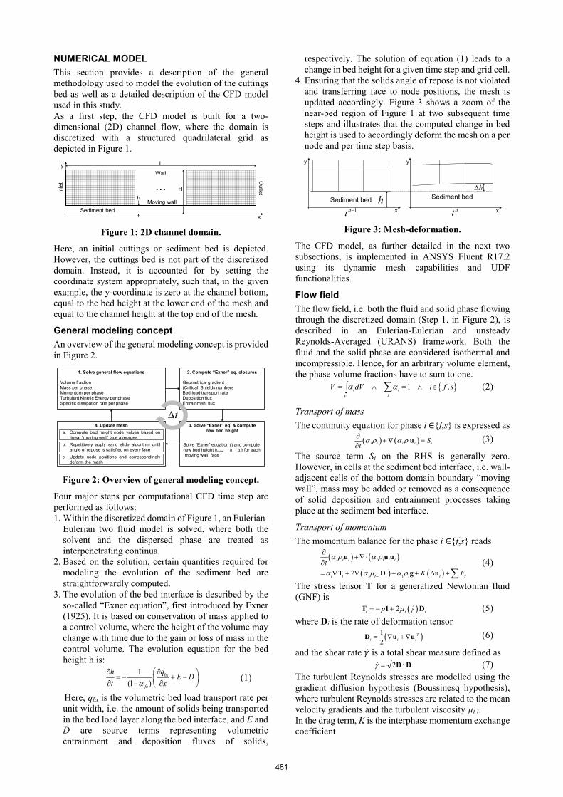
NUMERICAL MODEL This section provides a description of the general methodology used to model the evolution of the cuttings bed as well as a detailed description of the CFD model used in this study. As a first step, the CFD model is built for a two-dimensional (2D) channel flow, where the domain is discretized with a structured quadrilateral grid as depicted in Figure 1.

OutletIn

let

L

Hh

Wall

x

y

Sediment bed

…Moving wall

Figure 1: 2D channel domain.

Here, an initial cuttings or sediment bed is depicted. However, the cuttings bed is not part of the discretized domain. Instead, it is accounted for by setting the coordinate system appropriately, such that, in the given example, the y-coordinate is zero at the channel bottom, equal to the bed height at the lower end of the mesh and equal to the channel height at the top end of the mesh.

General modeling concept An overview of the general modeling concept is provided in Figure 2.

3. Solve “Exner” eq. & computenew bed height

2. Compute “Exner” eq. closures

4. Update mesh

Geometrical gradient(Critical) Shields numbersBed load transport rateDeposition fluxEntrainment flux

a. Compute bed height node values based onlinear “moving wall” face averages

1. Solve general flow equations

Solve “Exner” equation () and compute new bed height ℎ𝑛𝑒𝑤 = ℎ + ∆ℎ for each “moving wall” face

b. Repetitively apply sand slide algorithm untilangle of repose is satisfied on every face

c. Update node positions and correspondinglydeform the mesh

t∆

Volume fractionMass per phaseMomentum per phaseTurbulent Kinetic Energy per phaseSpecific dissipation rate per phase

Figure 2: Overview of general modeling concept.

Four major steps per computational CFD time step are performed as follows: 1. Within the discretized domain of Figure 1, an Eulerian-

Eulerian two fluid model is solved, where both the solvent and the dispersed phase are treated as interpenetrating continua.

2. Based on the solution, certain quantities required for modeling the evolution of the sediment bed are straightforwardly computed.

3. The evolution of the bed interface is described by the so-called “Exner equation”, first introduced by Exner (1925). It is based on conservation of mass applied to a control volume, where the height of the volume may change with time due to the gain or loss of mass in the control volume. The evolution equation for the bed height h is:

1

(1 )bx

fb

qh E Dt xα

∂∂ = − + − ∂ − ∂ (1)

Here, qbx is the volumetric bed load transport rate per unit width, i.e. the amount of solids being transported in the bed load layer along the bed interface, and E and D are source terms representing volumetric entrainment and deposition fluxes of solids,

respectively. The solution of equation (1) leads to a change in bed height for a given time step and grid cell.

4. Ensuring that the solids angle of repose is not violated and transferring face to node positions, the mesh is updated accordingly. Figure 3 shows a zoom of the near-bed region of Figure 1 at two subsequent time steps and illustrates that the computed change in bed height is used to accordingly deform the mesh on a per node and per time step basis.

Sediment bed

y

1nt −

h Sediment bedh∆

x x

y

nt Figure 3: Mesh-deformation.

The CFD model, as further detailed in the next two subsections, is implemented in ANSYS Fluent R17.2 using its dynamic mesh capabilities and UDF functionalities.

Flow field The flow field, i.e. both the fluid and solid phase flowing through the discretized domain (Step 1. in Figure 2), is described in an Eulerian-Eulerian and unsteady Reynolds-Averaged (URANS) framework. Both the fluid and the solid phase are considered isothermal and incompressible. Hence, for an arbitrary volume element, the phase volume fractions have to sum to one. { }1 ,i i i

iV

V dV i f sα α= ∧ = ∧ ∈∑∫ (2)

Transport of mass The continuity equation for phase i ∈{f,s} is expressed as ( ) ( )i i i i i iS

tα ρ α ρ∂

+ ∇ =∂

u (3)

The source term Si on the RHS is generally zero. However, in cells at the sediment bed interface, i.e. wall-adjacent cells of the bottom domain boundary “moving wall”, mass may be added or removed as a consequence of solid deposition and entrainment processes taking place at the sediment bed interface.

Transport of momentum The momentum balance for the phase i ∈{f,s} reads

( ) ( )

( ) ( )2

i i i i i i i

i i i t i i i i i s

tK F

α ρ α ρ

α α µ α ρ−

∂+ ∇ ⋅

∂= ∇ + ∇ + + ∆ + ∑

u u u

T D g u (4)

The stress tensor T for a generalized Newtonian fluid (GNF) is ( )2i i ip µ γ= − +T 1 D (5) where Di is the rate of deformation tensor ( )1

2T

i i i= ∇ + ∇D u u (6)

and the shear rate �̇�𝛾 is a total shear measure defined as 2 :γ = D D (7) The turbulent Reynolds stresses are modelled using the gradient diffusion hypothesis (Boussinesq hypothesis), where turbulent Reynolds stresses are related to the mean velocity gradients and the turbulent viscosity µt-i. In the drag term, K is the interphase momentum exchange coefficient

481

( )6

i sD

s

AK f cρτ

= (8)

with the particle relaxation time

18s s

sf

dρτµ

= (9)

and where the function f(cD) represents the effect of a particular interphase momentum exchange model. Here, the model of Schiller and Naumann (1933) has been used. Other momentum exchange terms include lift, virtual mass, turbulent dispersion and turbulent interaction L VM TD TIF F F F F= + + +∑ (10) where the standard Fluent formulation for the virtual mass force is used and lift is described by the model of Saffman (1965), turbulent dispersion by the model of Simonin and Viollet (1990b), and turbulent interaction as described by Simonin and Viollet (1990a). Note, that, in accordance with the source term in the mass transport equation (3), the momentum equation (4) should feature a corresponding momentum source term to account for momentum exchange in the wall-adjacent grid cells. However, compared to the other terms in equation (4), the momentum source term due to mass exchange is expected to be of negligible order of magnitude.

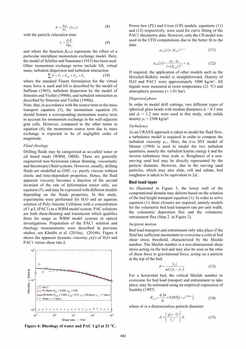
Fluid rheology Drilling fluids may be categorized as so-called water or oil based muds (WBM, OBM). These are generally engineered non-Newtonian (shear thinning, viscoelastic and thixotropic) fluid systems. However, usually, drilling fluids are modelled as GNF, i.e. purely viscous without elastic and time-dependent properties. Hence, the fluid apparent viscosity becomes a function of the second invariant of the rate of deformation tensor only, see equation (5), and may be expressed with different models depending on the fluids properties. In this study, experiments were performed for H2O and an aqueous solution of Poly-Anionic Cellulose with a concentration of 1 g/L (PAC1) as a WBM model system. PAC solutions are both shear-thinning and translucent which qualifies them for usage as WBM model systems in optical investigations. Preparation of the PAC1 solution and rheology measurements were described in previous studies, see Khatibi et al. (2016a), (2016b). Figure 4 shows the apparent dynamic viscosity µ(�̇�𝛾) of H2O and PAC1 versus shear rate �̇�𝛾.

Figure 4: Rheology of water and PAC 1 g/l at 21 °C.

Power-law (PL) and Cross (CR) models, equations (11) and (12) respectively, were used for curve fitting of the PAC1 rheometric data. However, only the CR model was used in the CFD computations due to the better fit to the data. ( ) 1PLn

PLPL Kµ γ γ −= (11)

( )( )

0 1 CRnCR

CRK∞

∞µ µµ γ µ

γ−

= ++

(12)

If required, the application of other models such as the Herschel-Bulkley model is straightforward. Density of H2O and PAC1 were approximately 1000 kg/m³. All liquids were measured at room temperature (21 °C) and atmospheric pressure (≈ 1.01 bar).

Dispersed phase In order to model drill cuttings, two different types of spherical glass beads with median diameters ds = 0.3 mm and ds = 1.2 mm were used in this study, with solids density ρs = 2500 kg/m³.

Turbulence As an URANS approach is taken to model the fluid flow, a turbulence model is required in order to compute the turbulent viscosity µt-i. Here, the k-ω SST model of Menter (1994) is used to model the two turbulent quantities, namely the turbulent kinetic energy k and the inverse turbulence time scale ω. Roughness of a non-moving sand bed may be directly represented by the particle diameter. However, due to the moving sand particles, which may also slide, roll and saltate, bed roughness is taken to be equivalent to 2ds.

Bed load layer As illustrated in Figure 3, the lower wall of the computational domain may deform based on the solution of the bed height transport equation (1). In order to solve equation (1), three closures are required, namely models for the volumetric bed load transport rate per unit width, the volumetric deposition flux and the volumetric entrainment flux (Step 2. in Figure 2).

Incipient motion Bed load transport and entrainment only take place if the fluid has sufficient momentum to overcome a critical bed shear stress threshold, characterized by the Shields number. The Shields number is a non-dimensional shear stress acting on the bed and may also be seen as the ratio of shear force to gravitational force, acting on a particle at the top of the bed.

( )b

s s fgdτ

θρ ρ

=−

(13)

For a horizontal bed, the critical Shields number to overcome for bed load transport and entrainment to take place, may be estimated using an empirical expression of Soulsby (1997)

( )*0.02,0

*

0.24 0.055 1 dcr e

dθ −= + − (14)

where d* is a dimensionless particle diameter

( )

13

* 2

1s

f

g sd d

ν −

=

(15)

482

Applying a force balance to a particle on a slope yields, for the 2D case, where shear stress always acts in the bed slope direction,

( )( ),0

sinsincr cr

β φθ θ

φ+

= (16)

where ϕ is the solids angle of repose and β is the local bed slope.

Bed load transport rate The bed load transport rate is mainly a function of the shear stress acting on the bed. Various empirical bed load formulas exist for different flow patterns and sediments. In this study, the expression of Nielsen (1992) is used,

( ) ( )0 3

0

12 1cr

bxs cr cr

ifq

g s d if

θ θ

θ θ θ θ θ−

≤= − − >

(17)

which is valid for a zero-slope bed. Following Struiksma and Crosato (1989), a slope correction term is introduced as

0f

bx bxf

u hq q Cxu−

∂ = − ∂

(18)

where C is a constant and the direction of qbx is assumed to be equivalent to the x-direction of the fluid velocity uf in the wall-adjacent grid cell.

Deposition The deposition flux D, i.e. particles leaving suspension and depositing on the bed, may be modeled as the product of the solid volume fraction and the suspension hindered settling velocity of Richardson and Zaki (1957) ( )n

s f setD vα α= (19) where vset is the settling velocity of an individual particle estimated with ( )4

3s f p

setf D

d gv

cρ ρ

ρ−

= − (20)

based on the drag coefficient cD of Schiller and Naumann (1933). According to Garside and Al-Dibouni (1977), the exponent n in equation (19) is given by

0.9

0.9

0.27 Re 5.10.1Re 1

p

p

n+

=+

(21)

Entrainment/Erosion Following Celik and Rodi (1988), the entrainment flux E, i.e. particles leaving the bed and entering suspension due to near-bed turbulent eddies, may be expressed with the near-bed Reynolds flux of solids

s j sT

s s T

uE

Sc yα αµ

ρ ρ

′ ′ ∂= ≈ −

∂ (22)

which may be modeled using the ratio of turbulent viscosity and the turbulent Schmidt number times the solid fraction gradient.

Sand slide A pile of granular material will, under the pure influence of gravity, settle in such a way that the angle between its slope and the horizontal plane is equal to the materials angle of repose. The solution of equation (1) may lead to a violation of the angle of repose. Hence, a sand slide algorithm is required to avoid local violation of the angle of repose. The algorithm of Liang et al. (2005) is applied, where a face gradient is readjusted in a mass-conservative manner if the face slope is violating the angle of repose (Step 4. in Figure 2).

Boundary and initial conditions Initially, the bed height is 5 mm in the entire domain and all the flow variables in the domain are zero. At the inlet, a laminar velocity profile, which is adjusted to the potentially changing inlet size between step (4) and step (1) in Figure 2, is utilized for both the solid and the fluid phase. The velocity profile is defined in such a manner that the superficial velocities of the 2D channel flow CFD model and 3D pipe flow experiments match. A zero bed load transport rate gradient is used as a BC for the volumetric bed load transport rate. The solid volume fraction is assumed constant across the inlet. Reasonable values for the in-situ solid volume fraction were estimated based on the ratio of experimental superficial velocities

sss

ss sl

UU U

α =+

(23)

where the superficial particle velocity was calculated from the solids collection/injection rate and the superficial liquid velocity was calculated based on logged data from a Coriolis flow meter.

Implementation in ANSYS Fluent R17.2 With reference to Figure 2, the implementation in ANSYS Fluent R17.2 is as follows: 1. The flow field is solved in a standard manner using the

Phase-Coupled SIMPLE scheme, spatial discretization is second order, with the exception of volume fraction where the QUICK scheme has been used. The time discretization is implicit second order.

2. After the flow field variables are available, the three closures (18), (19), and (22) are calculated using an EXECUTE_AT_END UDF.

3. In the same UDF, the bed height evolution equation (1) is solved with a first-order upwind scheme

( ) ( )(1 ) (1 )

t t t t tx x x x x

fb fb

t th h q q E Dxα α

+∆−∆

∆− −

∆= − − − −

∆ (24)

Note, that the volumetric transport rate qx is a function of the transported property h. However, changes of the bed height h occur on a much larger time scale than changes of flow field variables such as velocity. Since the first-order upwind scheme, i.e. equation (24), is solved at the end of each CFD time step, no numerical instabilities are to be expected. The net solid and fluid fluxes into/out of the wall-adjacent cell leads to a source term in these cells, as given in equation (3).

4. Finally, the computational domain is then updated by individual node movement using a DEFINE_GRID_MOTION UDF, where the new node positions are computed based on linear face position averages and the whole bed is repetitively swept with the sand slide algorithm until the angle of repose is satisfied at all bed faces. ANSYS Fluent's dynamic mesh capability is used to deform the mesh correspondingly. Here, the spring-based smoothing method is used, where the individual node displacements are obtained by treating the mesh as a network of connected springs. Displacements of the boundary nodes computed via equation (24) will be transmitted through the mesh by calculating adjacent node displacements based on Hooke’s law.

483

EXPERIMENTS

Flow loop The experiments were carried out in a medium-scale flow loop at the University of Stavanger. The flow loop, shown in Figure 5, is a closed loop, where the particles are separated and re-injected continuously to the test sections after collection in a hydrocyclone (10).

Figure 5: Medium-scale flow loop.

The flow loop features both a horizontal and an inclined test section, where the pipe is made of transparent plexiglas. The inner pipe diameter is 0.04 m, the total length of the horizontal test section is 6 m, with an upstream entrance length of 4 m. The test fluid was stored in a 350 L source tank (1). A PCM Moineau 2515 screw pump (2), regulated by a frequency invertor, provided the flow. Liquid flow rate and temperature were monitored by a Promass 80F DN50 Coriolis flow meter (3). The glass beads were mixed into the liquid through a Venturi shaped injector (4). The test section was located 4 m downstream of the injection point to minimize entrance flow effects and to let the particle-liquid patterns become fully developed. The pressure gradient data was measured over a length of 1.52 m by a Rosemount 3051 transducer (9). At the same position, flow pattern images were recorded using two high speed video cameras (8): A Basler camera with 500 fps at full resolution of 800x600 and a SpeedCam Mini e2 camera with 2500 fps at full resolution of 512x512 pixels. Particles and liquid were separated in the hydrocyclone (10), just after the inclined test section. The particles are then re-injected through the injection pipe (7) and the liquid is returned to the tank (1).

Estimate of CFD boundary conditions The solid superficial velocity required to specify the in-situ solid volume fraction used as a BC in the CFD model, i.e. equation (23), was estimated by measuring the injection and collection rate of particles. A time series of images of the injection pipe (7) was obtained, where one of the control valves (5, 6) was closed and the other one was open to collect or inject the particles. The changes of the packed particles height were calculated by analyzing the images in Matlab.

Test matrix Table 1 summarizes the relevant parameters used in the experiments (and corresponding simulations). In all cases, glass beads with a density of 2500 kg/m³ were used as solids. The global αs represents the total volumetric loading of solids in the flow loop, whereas the in-situ αs represents the estimated solid volume fraction of moving solids

according to equation (23) used as a BC in the CFD simulations.

Table 1: Test matrix

Case #1 #2 #3 #4 #5 Fluid H2O H2O H2O PAC1 PAC1

Usl [m/s] 0.26 0.43 0.44 0.45 0.81 µ0 [mPa.s] - - - 26 26 µ∞ [mPa.s] 1 1 1 1 1

KCR [Pa.snCR] - - - 0.008 0.008 nCR [-] - - - 0.37 0.37

ds [mm] 0.3 0.3 1.2 1.2 1.2 αS [-] global 0.08 0.08 0.12 0.12 0.12 αS [-] in-situ ≈ 0.0015 ≈ 0.0015 ≈ 0.001 ≈ 0.001 ≈ 0.001

Pipe inclination was 0° in all cases, i.e. only the data from the horizontal test section was used in this study.

RESULTS

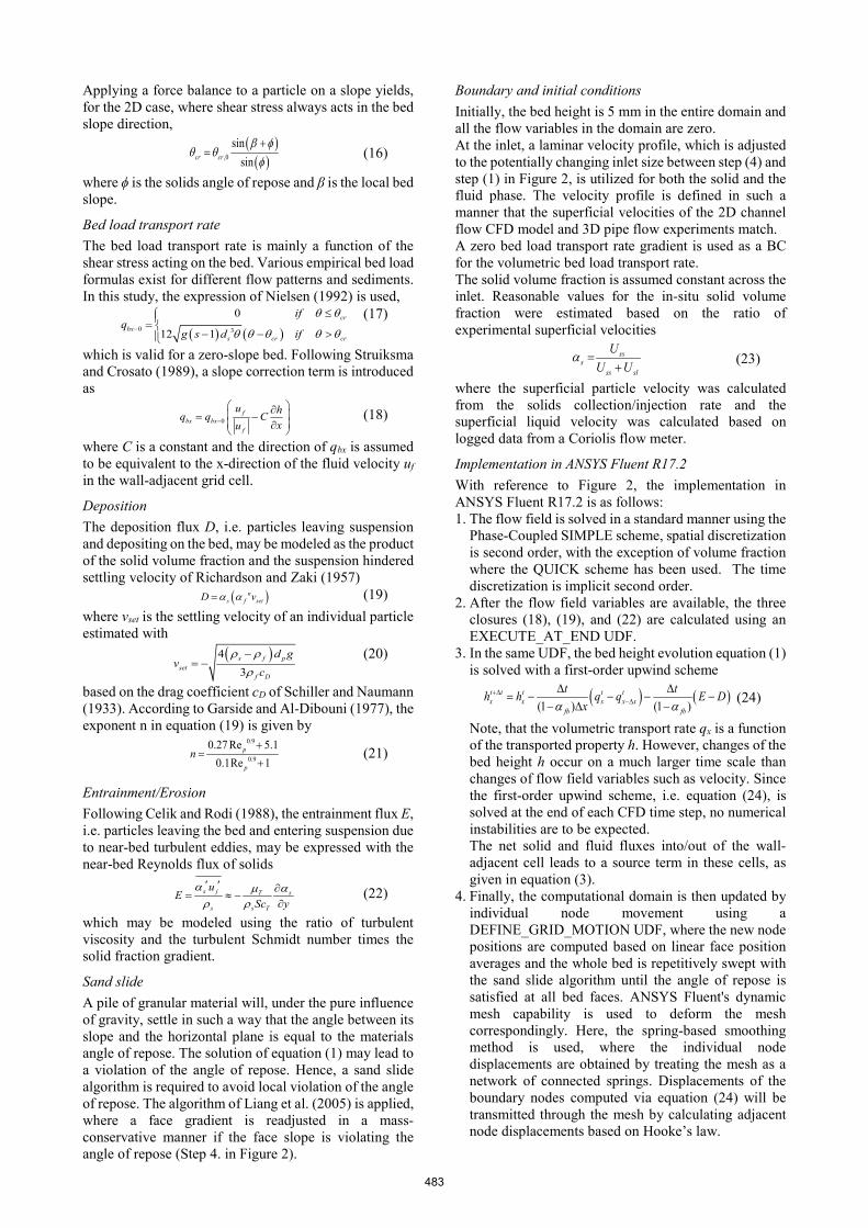
Numerical Modeling (CFD) In the case of H2O, solids eventually accumulate into a pile at the inlet due to a developing recirculation zone, blocking more than half the inlet. For case #1, as depicted in Figure 6, and at approximately x ≈ 1 m, a static bed begins to form where the solids concentration profile as well as the bed height is constant with respect to x.

Figure 6: Bed height as a function of time, case #1.

For case #2, as illustrated in Figure 7, a large pile of solids develops in the domain (here depicted at t = 50 s), which eventually is eroded.


For case #3, simulations were always diverging for a big variety of solver settings. Using time steps < 0.0005 s lead to stable simulations; however, no results were obtained due to currently unavailable computational power required.

484

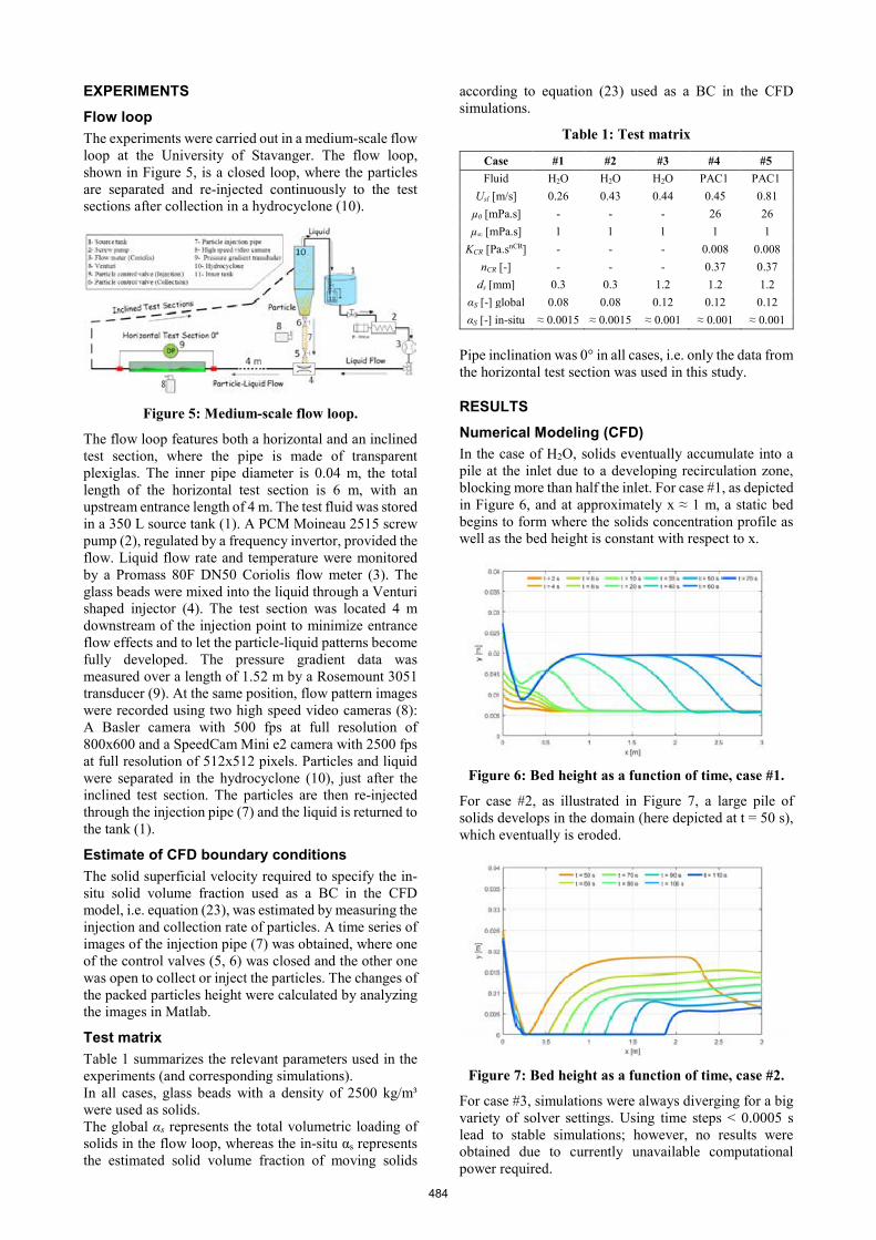
In case of PAC1, no pile build-up is observed at the inlet in either case. For case #4, as depicted in Figure 8, a dune starts to grow at x ≈ 0.5 m and eventually the bed approaches a steady-state with a bed height h = 0. 0136 m.


For case #5, as illustrated in Figure 9, the bed is eroded from the start and yields a semi-steady-state bed height towards the outlet.


However, the bed is eroded continuously, leading to zero bed height after the small dune traveling through the domain in the flow wise direction. No moving sand dunes were observed in the simulations.

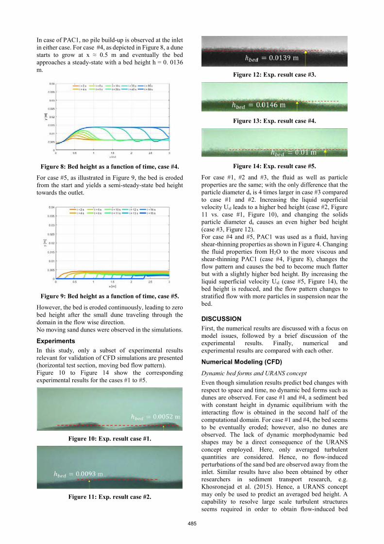
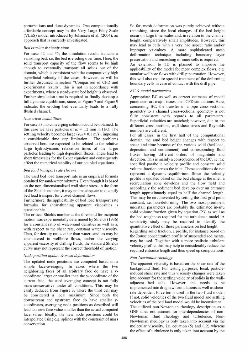
Experiments In this study, only a subset of experimental results relevant for validation of CFD simulations are presented (horizontal test section, moving bed flow pattern). Figure 10 to Figure 14 show the corresponding experimental results for the cases #1 to #5.

Figure 10: Exp. result case #1.





For case #1, #2 and #3, the fluid as well as particle properties are the same; with the only difference that the particle diameter ds is 4 times larger in case #3 compared to case #1 and #2. Increasing the liquid superficial velocity Usl leads to a higher bed height (case #2, Figure 11 vs. case #1, Figure 10), and changing the solids particle diameter ds causes an even higher bed height (case #3, Figure 12). For case #4 and #5, PAC1 was used as a fluid, having shear-thinning properties as shown in Figure 4. Changing the fluid properties from H2O to the more viscous and shear-thinning PAC1 (case #4, Figure 8), changes the flow pattern and causes the bed to become much flatter but with a slightly higher bed height. By increasing the liquid superficial velocity Usl (case #5, Figure 14), the bed height is reduced, and the flow pattern changes to stratified flow with more particles in suspension near the bed.

DISCUSSION First, the numerical results are discussed with a focus on model issues, followed by a brief discussion of the experimental results. Finally, numerical and experimental results are compared with each other.

Numerical Modeling (CFD)

Dynamic bed forms and URANS concept Even though simulation results predict bed changes with respect to space and time, no dynamic bed forms such as dunes are observed. For case #1 and #4, a sediment bed with constant height in dynamic equilibrium with the interacting flow is obtained in the second half of the computational domain. For case #1 and #4, the bed seems to be eventually eroded; however, also no dunes are observed. The lack of dynamic morphodynamic bed shapes may be a direct consequence of the URANS concept employed. Here, only averaged turbulent quantities are considered. Hence, no flow-induced perturbations of the sand bed are observed away from the inlet. Similar results have also been obtained by other researchers in sediment transport research, e.g. Khosronejad et al. (2015). Hence, a URANS concept may only be used to predict an averaged bed height. A capability to resolve large scale turbulent structures seems required in order to obtain flow-induced bed

485

perturbations and dune dynamics. One computationally affordable concept may be the Very Large Eddy Scale (VLES) model introduced by Johansen et al. (2004), an approach that is currently investigated.

Bed erosion & steady-state For case #2 and #5, the simulation results indicate a vanishing bed, i.e. the bed is eroding over time. Here, the solid transport capacity of the flow seems to be high enough to eventually transport all solids out of the domain, which is consistent with the comparatively high superficial velocity of the cases. However, as will be further discussed in section “Comparison of CFD and experimental results”, this is not in accordance with experiments, where a steady-state bed height is observed. Further simulation time is required to finally develop a full dynamic equilibrium, since, as Figure 7 and Figure 9 indicate, the eroding bed eventually leads to a fully flushed channel.

Numerical instabilities For case #3, no converging solution could be obtained. In this case we have particles of ds = 1.2 mm in H2O. The settling velocity becomes large (vset ≈ 0.1 m/s), imposing a considerable time step limitation. The problems observed here are expected to be related to the relative large hydrodynamic relaxation times of the larger particles leading to high deposition fluxes. These lead to short timescales for the Exner equation and consequently affect the numerical stability of our coupled equations.

Bed load transport rate closure The used bed load transport rate is an empirical formula obtained for sand-water mixtures. Even though it is based on the non-dimensionalised wall shear stress in the form of the Shields number, it may not be adequate to quantify bed load transport for closed channel flows. Furthermore, the applicability of bed load transport rate formulas for shear-thinning apparent viscosities is questionable. The critical Shields number as the threshold for incipient motion was experimentally determined by Shields (1936) for a constant ratio of water-sand densities as well as a, with respect to the shear rate, constant water viscosity. Thus, for density ratios other than water-sand, as may be encountered in wellbore flows, and/or the varying apparent viscosity of drilling fluids, the standard Shields curve may not represent the correct threshold of motion.

Node position update & mesh deformation The updated node positions are computed based on a simple face-averaging. In cases where the two neighboring faces of an arbitrary face do have a y-coordinate larger or smaller than the y-coordinate of the current face, the used averaging concept is not fully mass-conservative under all conditions. This may be easily deduced from Figure 3, where the third cell may be considered a local maximum. Since both the downstream and upstream face do have smaller y-coordinates, averaging node positions as described will lead to a new face value smaller than the actual computed face value. Ideally, the new node positions could be interpolated using e.g. splines with the constraint of mass conservation.

So far, mesh deformation was purely achieved without remeshing, since the local changes of the bed height occur on large time scales and, in relation to the channel height, comparatively small amplitudes. However, this may lead to cells with a very bad aspect ratio and/or improper y+-values. A more sophisticated mesh deformation technique including boundary layer preservation and remeshing of inner cells is required. An extension to 3D is planned to improve the applicability of the model for more complex flows, e.g. annular wellbore flows with drill pipe rotation. However, this will also require special treatment of the deforming boundary cells in case of contact with the drill pipe.

BC & model parameters Appropriate BC as well as correct estimates of model parameters are major issues in all CFD simulations. Here, concerning BC, the transfer of a pipe cross-sectional geometry to a channel cross-sectional geometry is not fully consistent with regards to all parameters: Superficial velocities are matched; however, due to the different cross-sections, wall shear stress and Reynolds numbers are different. For all cases, in the first half of the computational domain, the sand bed height changes with respect to space and time because of the various solid (bed load, deposition and entrainment) and corresponding fluid fluxes having different orders of magnitude and direction. This is mainly a consequence of the BC, i.e. the specified parabolic velocity profile and constant solid volume fraction across the inlet. These conditions do not represent a dynamic equilibrium. Since the velocity profile is updated based on the bed change at the inlet, a recirculation zone develops and the flow field and accordingly the sediment bed develop over an entrance length approximately equal to half the channel length. This may be circumvented by setting the first grid point constant, i.e. non-deforming. The two most prominent uncertain parameters are probably the estimated in-situ solid volume fraction given by equation (23) as well as the bed roughness required for the turbulence model. A sensitivity study may be required to identify the quantitative effect of these parameters on bed height. Regarding solid fraction, a profile, for instance based on the Rouse concentration profile of suspended sediments, may be used. Together with a more realistic turbulent velocity profile, this may help to considerably reduce the required entrance length and thus speed up computations.

Non-Newtonian rheology The apparent viscosity is based on the shear rate of the background fluid. For testing purposes, local, particle-induced shear rate and thus viscosity changes were taken into account for the settling velocity of solids in the wall-adjacent bed cells. However, this needs to be implemented into drag law formulations as well as shear-rate dependent force terms used in the two-fluid model. If not, solid velocities of the two fluid model and settling velocities of the bed load model would be inconsistent. The utilized non-Newtonian rheology description as a GNF does not account for interdependencies of non-Newtonian fluid rheology and turbulence. Non-Newtonian rheology is only taken into account via the molecular viscosity, i.e. equation (5) and (12) whereas the effect of turbulence is only taken into account by the

486

corresponding models affecting the turbulent viscosity µt-i. This is due to the conventional but simplified RANS treatment where the viscosity is first considered constant and later made variable by relating it to the shear rate, again see equation (5) and (12). Thus, terms representing the impact of fluctuations in strain rate on the fluids molecular viscosity as shown by Pinho (2003) as well as Gavrilov and Rudyak (2016) are ignored. Adequate wall treatment for non-Newtonian fluids is not available so far, as the wall functions in ANSYS Fluent are based on the common Newtonian log-law concept. Hence, the boundary layer needs to be resolved down to y+ < 1 into the laminar sublayer or non-Newtonian wall laws have to be developed, e.g. based on Johansen (2015). Drag, other momentum exchange terms and settling models utilized are based on Newtonian fluids. Here, further work is needed to account for non-constant viscosities, using available modeling concepts such as e.g. Childs et al. (2016); Ceylan et al. (1999); Li et al. (2012); Renaud et al. (2004); Shah et al. (2007); Shah (1986).

Experiments Recording of experimental data started after a flow stabilization sequence of 30 min, in order to yield dynamic equilibrium. An entrance length of 4 m upstream of the test section was sufficient to yield a well- developed particle-liquid flow in test section of the horizontal pipe, where the video images were recorded. The camera frame rate was sufficient to capture and track the movement of individual particles inside the test section. Bed heights were measured from the video images and are in agreement with conventional theory. Theoretically, the bed height should decrease with increasing liquid flowrate due to increased shear stress against the bed. Thus, both bed load and suspended load increase, which may be directly seen in Figure 13 and Figure 14 for the case of PAC1. However, in the case of H2O, an increase in bed height is observed, which may be explained by flow pattern transition from a rather stationary bed, where dunes are moving very slowly (case #1) to a moving bed, where dunes move much faster (case #2). In addition, beyond a threshold velocity, particle dunes disappear and the bed becomes flatter. For constant particle mass density, the bed height increases with increasing particle diameter, due to increase in settling velocity, and decrease in entrainment rate. Increased viscosity of shear-thinning fluid leads to decrease in bed height due to the increased solids transport capacity of the flow. This is mainly due to reduced settling velocity and consequently less deposition. It also leads to higher shear-stress acting on the bed and consequently more bed-load transport.

Comparison of CFD and experimental results As pointed out, the URANS-based numerical modeling approach does not yield any bed dynamics such as dunes. Therefore, comparison of CFD and experimental results may only be conducted based on a time/spatial average of the steady-state bed height.

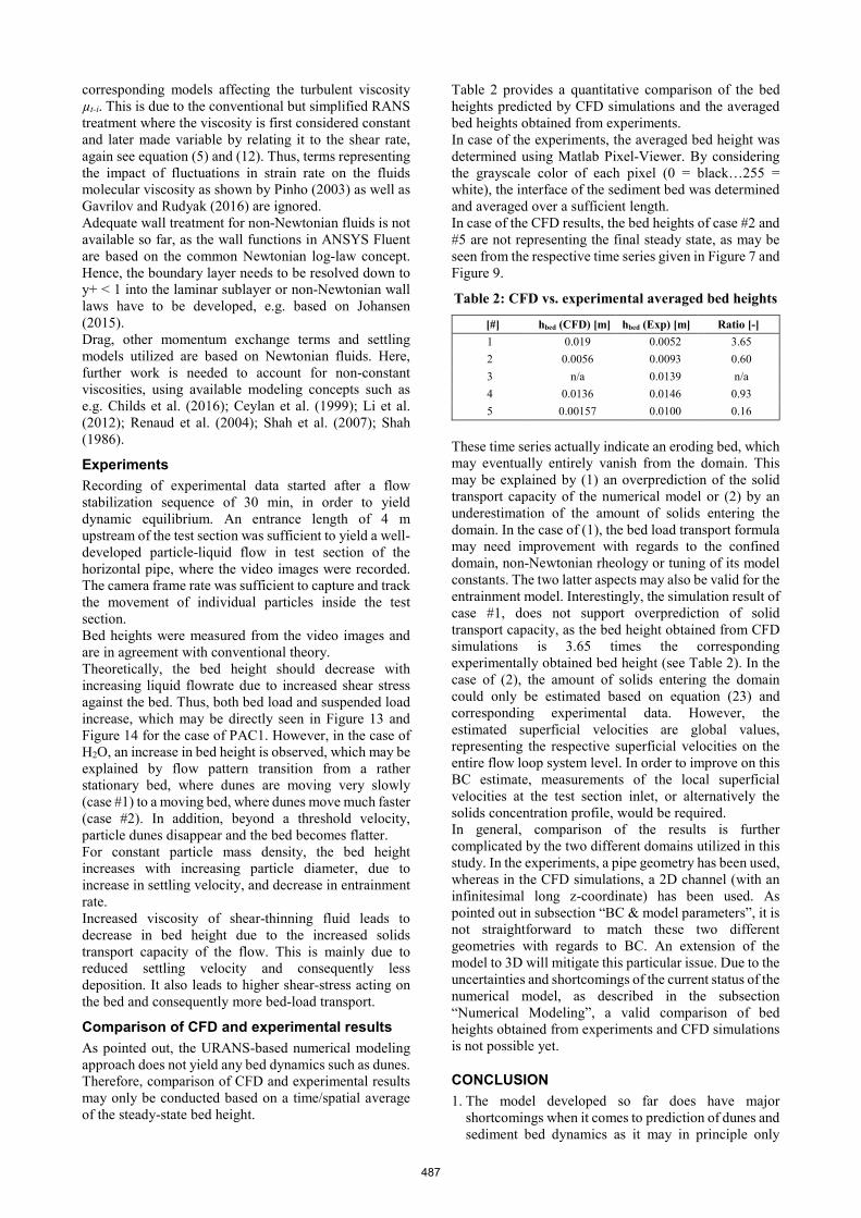
Table 2 provides a quantitative comparison of the bed heights predicted by CFD simulations and the averaged bed heights obtained from experiments. In case of the experiments, the averaged bed height was determined using Matlab Pixel-Viewer. By considering the grayscale color of each pixel (0 = black…255 = white), the interface of the sediment bed was determined and averaged over a sufficient length. In case of the CFD results, the bed heights of case #2 and #5 are not representing the final steady state, as may be seen from the respective time series given in Figure 7 and Figure 9.

Table 2: CFD vs. experimental averaged bed heights

[#] hbed (CFD) [m] hbed (Exp) [m] Ratio [-] 1 0.019 0.0052 3.65 2 0.0056 0.0093 0.60 3 n/a 0.0139 n/a 4 0.0136 0.0146 0.93 5 0.00157 0.0100 0.16

These time series actually indicate an eroding bed, which may eventually entirely vanish from the domain. This may be explained by (1) an overprediction of the solid transport capacity of the numerical model or (2) by an underestimation of the amount of solids entering the domain. In the case of (1), the bed load transport formula may need improvement with regards to the confined domain, non-Newtonian rheology or tuning of its model constants. The two latter aspects may also be valid for the entrainment model. Interestingly, the simulation result of case #1, does not support overprediction of solid transport capacity, as the bed height obtained from CFD simulations is 3.65 times the corresponding experimentally obtained bed height (see Table 2). In the case of (2), the amount of solids entering the domain could only be estimated based on equation (23) and corresponding experimental data. However, the estimated superficial velocities are global values, representing the respective superficial velocities on the entire flow loop system level. In order to improve on this BC estimate, measurements of the local superficial velocities at the test section inlet, or alternatively the solids concentration profile, would be required. In general, comparison of the results is further complicated by the two different domains utilized in this study. In the experiments, a pipe geometry has been used, whereas in the CFD simulations, a 2D channel (with an infinitesimal long z-coordinate) has been used. As pointed out in subsection “BC & model parameters”, it is not straightforward to match these two different geometries with regards to BC. An extension of the model to 3D will mitigate this particular issue. Due to the uncertainties and shortcomings of the current status of the numerical model, as described in the subsection “Numerical Modeling”, a valid comparison of bed heights obtained from experiments and CFD simulations is not possible yet.

CONCLUSION 1. The model developed so far does have major

shortcomings when it comes to prediction of dunes and sediment bed dynamics as it may in principle only

487

predict the steady-state average bed height due to the utilized URANS approach. A simplified LES approach, e.g. the VLES concept currently investigated, may lead to a model capable of describing flow-induced dynamic bed shapes such as travelling dunes.

2. The current model status does not correctly predict the transport capacity of the flow, i.e. does not allow a quantitatively correct prediction of the steady-state bed height. An improved bed load transport model, together with a more realistic entrainment model, may yield more realistic transport capacities and consequently better predict the steady-state bed shape and bed height.

3. Improved inlet boundary conditions, in particular an inlet turbulent velocity profile together with a solid volume fraction profile, may considerably shorten entrance length effects and consequently speed up computations.

4. Further modeling work is required to adequately describe the effect of non-Newtonian rheology on various elements of the model: Non-Newtonian formulations for closures such as the bed load formula, the drag coefficient, the (critical) Shields number, and the hindered settling effect as well as non-Newtonian turbulence interdependencies may improve the model.

5. An investigation of the model’s sensitivity with respect to bed roughness and in-situ solid volume fraction at the inlet is necessary in order to understand the effect of these two uncertain parameters.

6. An extension of the model to 3D will extend the applicability of the model for pipe flows, annular flows and potentially even more complex flows such as annular wellbore flows with drill pipe rotation, but at the same time require more sophisticated mesh deformation techniques.

ACKNOWLEDGEMENTS The project Advanced Wellbore transport Modelling (AdWell) with its sponsor, the Research Council of Norway and its partners Statoil, GDF SUEZ E&P Norge, IRIS, UiS, NTNU and SINTEF are gratefully acknowledged for funding and supporting part of this work.

REFERENCES BELLO, K. O. ET AL., (2011), “Minimum Transport Velocity Models for Suspended Particles in Multiphase Flow Revisited.” In SPE Annual Technical Conference and Exhibition Society of Petroleum Engineers. BRØRS, B., (1999), “Numerical Modeling of Flow and Scour at Pipelines.” Journal of Hydraulic Engineering 125:511–523. CELIK, I., AND RODI, W., (1988), “Modeling Suspended Sediment Transport in Nonequilibrium Situations.” Journal of Hydraulic Engineering 114:1157–1191. CEYLAN, K. ET AL., (1999), “A theoretical model for estimation of drag force in the flow of non-newtonian fluids around spherical solid particles.” Powder Technology 103:286–291. CHILDS, L. H. ET AL., (2016), “Dynamic settling of particles in shear flows of shear-thinning fluids.” Journal of Non-Newtonian Fluid Mechanics 235:83–94.

CORREDOR, R. ET AL., (2016), “Experimental investigation of cuttings bed erosion in horizontal wells using water and drag reducing fluids.” Journal of Petroleum Science and Engineering 147:129–142. DORON, P., AND BARNEA, D., (1993), “A three-layer model for solid-liquid flow in horizontal pipes.” International Journal of Multiphase Flow 19:1029–1043. EXNER, F. M., (1925), “Uber die Wechselwirkung zwischen Wasser und Geschiebe in Flüssen.” Akad. Wiss. Wien Math. Naturwiss. Klasse 134:165–204. GARSIDE, J., AND AL-DIBOUNI, M. R., (1977), “Velocity-Voidage Relationships for Fluidization and Sedimentation in Solid-Liquid Systems.” Industrial & Engineering Chemistry Process Design and Development 16:206–214. GAVRILOV, A. A., AND RUDYAK, V. Y., (2016), “Reynolds-averaged modeling of turbulent flows of power-law fluids.” Journal of Non-Newtonian Fluid Mechanics 227:45–55. GOHARZADEH, A. ET AL., (2013), “Experimental Characterization of Slug Flow on Solid Particle Transport in a 1 Deg Upward Inclined Pipeline.” Journal of Fluids Engineering 135:081304. HAN, S. M. ET AL., (2010), “Solid-liquid hydrodynamics in a slim hole drilling annulus.” Journal of Petroleum Science and Engineering 70:308–319. JOHANSEN, S. T., (2015), “Improved fluid control by proper non-Newtonian flow modeling.” In Tekna – Flow Assurance Larvik. JOHANSEN, S. T. ET AL., (2004), “Filter-based unsteady RANS computations.” International Journal of Heat and Fluid Flow 25:10–21. KHATIBI, M. ET AL., (2016a), “Experimental Investigation of Effect of Salts on Rheological Properties of Non-Newtonian Fluids.” In Nordic Rheology Conference, University of Helsinki, Finland. KHATIBI, M. ET AL., (2016b), “Particles Falling Through Viscoelastic Non-Newtonian Flows in a Horizontal Rectangular Channel Analyzed with PIV and PTV Techniques.” Journal of Non-Newtonian Fluid Mechanics 235:143–153. KHOSRONEJAD, A. ET AL., (2011), “Curvilinear immersed boundary method for simulating coupled flow and bed morphodynamic interactions due to sediment transport phenomena.” Advances in Water Resources 34:829–843. KHOSRONEJAD, A. ET AL., (2015), “Numerical simulation of large dunes in meandering streams and rivers with in-stream rock structures.” Fluvial Eco-Hydraulics And Morphodynamics 81:45–61. KHOSRONEJAD, A., AND SOTIROPOULOS, F., (2014), “Numerical simulation of sand waves in a turbulent open channel flow.” Journal of Fluid Mechanics 753:150–216. LI, S. ET AL., (2012), “The viscosity distribution around a rising bubble in shear-thinning non-newtonian fluids.” Brazilian Journal of Chemical Engineering 29:265–274. LIANG, D. ET AL., (2005), “Numerical modeling of flow and scour below a pipeline in currents - Part II. Scour simulation.” Coastal Engineering 52:43–62. MANZAR, M. A., AND SHAH, S. N., (2014), “Particle Distribution and Erosion During the Flow of Newtonian and Non-Newtonian Slurries in Straight and Coiled

488

http://www.ad-well.no/

http://www.ad-well.no/

Pipes.” Engineering Applications of Computational Fluid Mechanics 3:296–320. MENTER, F. R., (1994), “Two-equation eddy-viscosity turbulence models for engineering applications.” AIAA Journal 32:1598–1605. NIELSEN, P., (1992), “Coastal bottom boundary layers and sediment transport.” World Scientific Publishing Co Inc. NOSSAIR, A. M. ET AL., (2012), “Influence of Pipeline Inclination on Hydraulic Conveying of Sand Particles.” In ASME 2012 International Mechanical Engineering Congress and Exposition pp. 2287–2293. American Society of Mechanical Engineers. OFEI, T. N. ET AL., (2014), “CFD Method for Predicting Annular Pressure Losses and Cuttings Concentration in Eccentric Horizontal Wells.” Journal of Petroleum Engineering 2014:1–16. PINHO, F. T., (2003), “A Model for the Effect of Turbulence on the Molecular Viscosity of Generalized Newtonian Fluids.” In 17th International Congress of Mechanical Engineering, Brazilian Society of Mechanical Sciences and Engineering (ABCM), Sao Paulo. RENAUD, M. ET AL., (2004), “Power-Law Fluid Flow Over a Sphere: Average Shear Rate and Drag Coefficient.” The Canadian Journal of Chemical Engineering 82:1066–1070. RICHARDSON, J. F., AND ZAKI, W. N., (1957), “Sedimentation and fluidisation: Part I.” Chemical Engineering Research and Design 75:S82–S100. SAFFMAN, P. G., (1965), “The lift on a small sphere in a slow shear flow.” Journal of Fluid Mechanics 22:385. SAVAGE, S. B. ET AL., (1996), “Solids transport, separation and classification.” Powder technology 88:323–333. SCHILLER, L., AND NAUMANN, A., (1933), “Über die grundlegenden Berechnungen bei der

Schwerkraftaufbereitung.” Z. Ver. Dtsch. Ing 77:318–320. SHAH, S. N., (1986), “Proppant-settling correlations for non-Newtonian Fluids.” SPE Production Engineering 1:446–448. SHAH, S. N. ET AL., (2007), “New model for single spherical particle settling velocity in power law (visco-inelastic) fluids.” International Journal of Multiphase Flow 33:51–66. SHIELDS, A., (1936), “Anwendung der Aehnlichkeitsmechanik und der Turbulenzforschung auf die Geschiebebewegung.” SIMONIN, C., AND VIOLLET, P., (1990a), “Predictions of an oxygen droplet pulverization in a compressible subsonic coflowing hydrogen flow.” Numerical Methods for Multiphase Flows, FED91:65–82. SIMONIN, O., AND VIOLLET, P., (1990b), “Modelling of turbulent two-phase jets loaded with discrete particles.” FG Hewitt, et al., Phenomena in multiphase yow:259. SOLBERG, T. ET AL., (2006), “CFD modelling of scour around offshore wind turbines in areas with strong currents.” In Offshore Wind Turbines situated in Areas with Strong Currents Offshore Center Danmark, Esbjerg. SOULSBY, R., (1997), “6. Threshold of motion.” In Dynamics of marine sands pp. 97–110. Thomas Telford Publishing. STRUIKSMA, N., AND CROSATO, A., (1989), “Analysis of a 2-D bed topography model for rivers.” In Water Resources Monograph (S. Ikeda and G. Parker, eds.) pp. 153–180. American Geophysical Union, Washington, D. C. SUN, X. ET AL., (2014), “Effect of drillpipe rotation on cuttings transport using computational fluid dynamics (CFD) in complex structure wells.” Journal of Petroleum Exploration and Production Technology 4:255–261.

489

Documents

Progress in Applied CFD – CFD2017