Programming under uncertainty: The complete problem

Z. Wahrscheinliehkeitstheorie verw. Geb. 4, 316--339 (1966)

Programming under Uncertainty: The (~omplete Problem ~ l~oaw~ W~Ts

Received December 3, 1964

Abstract. We define the complete problem of a two-stage linear programming under uncertainty, to be:

Minimize z(x) = E~(cx ~ q+y+ ~ q-y-} subject to A x = b

Tx + I y + ~- I y - = x~O,y+ ~=O,y-~O

where x is the first-stage decision variable, the pair (y+, y-) represents the second-stage decision variables. In order to solve this class of problem, we derive a convex programming problem, whose set of optimal solutions is identical to the set of optimal solutions of our original problem. This problem is called the effuivalent convex programming. If the random variable has a continuous distribution, we give an algorithm to solve the equivalent convex program. Moreover, we derive explicitly the equivalent convex program for a few common distributions.

1. Introduction

The standard/orm for the two-stage l inear program under unce r t a in ty is :

(1) Minimize z(x) = E~{cx -~ q y} subject to A x =- b

T x - ~ M y = - ~ ~ ( ~ , Y , F ) x~=O y>=O

where A is a mat r ix m • n, T is n5 • n, M is ~ • ~, ~ is a r andom vector whose

probabi l i ty space is (~, ~ , F). This problem (1) belongs to the class of stochastic l inear programming problems for which one seeks a here-and-now 8olution. One interprets problem (1) as follows: the decision maker selects the ac t iv i ty levels for

x, say x --~ ~, he then observes the r andom event $ ~ ~ and he is finally allowed a

corrective act ion y, such t h a t y ~_ O, M y ~ ~ -- T~ and qy is m in imum. This second stage decision y, is t aken when no "uncertaint ies , , are left in the problem.

The decision maker wants to minimize the sum of his fixed costs (cx) a nd of the pena l ty costs he m a y expect when he has selected given ac t iv i ty levels (x). I t is clear from this in te rpre ta t ion t ha t we could also write the objective funct ion of (1)

(2) z(x) ~-- cx -~ E ~ ( m i n q y [ x } .

All quant i t ies considered here belong to the reals, denoted R. Vectors will belong to f ini te-dimensional real vector spaces R n and whether they are to be regarded as row vectors or column vectors will always be dea r from the context in

* Parts of this material was written while the author was at the Operations Research Center at the University of California (Berkeley), where this research was partially supported by the Office of Naval Research under Contract Number 222 (83) with the University of Cali- fornia and by a research grant from the National Science Foundation.

Programming under Uncertainty: The Complete Problem 317

which they appear. Thus, for example, the expressions

Z = (Zl, .-. , Zi, -. . , Z~)

T x = Z ~a

y+v- = v2 y7 i=1

are easily understood. No special provisions will be made for transposing vectors. The random vector ~ : (~l . . . . . ~i, . . . , ~ ) is a "numerical" random vector,

i.e. E c R ~, ~ is a ~-algebra and F is a probabili ty distribution function from which could be obtained a probabili ty measure. (31, ~-l , F/) is the probabili ty space of the random variable ~ . We only need independence of ~ and x : our first- stage decision has no effect on (~, ~ , F).

I f for every finite interval, Fi (~) has a finite number of discontinuity points, then we can always integrate by parts ]gl(~i)dFt(~i), where g~($i) is a linear function of $i. I f it exists, we denote the density function of ~i by / i (~i) i = 1 . . . . . and ff they exist, let ~ / a n d fli be respectively the greatest lower bound and least upper bound of $/. We assume tha t E~,{~i} exists for all i ---- 1, . . . , ~ .

We say tha t problem (1) is Complete when the matr ix M (after an appropriate rearrangement of rows and columns) can be partit ioned in two parts, whose first part is an identity matr ix and the second par t is the negative of an identi ty matrix, M = (I, - - I) .

The standard form of the problem to be studied in this article is then

(3) Minimize z(x) = E~ {cx + q+ y+ + q-y-} subject to A x = b

T x + I y + - - I y - = ~ , ~ e ( S , , ~ , Y ) x>=O, y+>=O, y->=O

where we parti t ioned the vectors q and y of the standard form (1) in (q+, q-) and (y+, y-), respectively. I f m = 0 (i. e. there are no constraints of type A x -= b) the characteristics of our problem remain the same.

Among all classes of special cases of the two-stage linear programs under uncertainty, the "complete,, case seems to cover the largest class of possible applications. One can think of the vector x as representing the activity levels of a production plant, constrained by A x = b, x ~ 0. T is the " transformation" of these act ivi ty levels into sellable goods. Z = Tx, is then the amount of goods the producer decides to place on a market where the demand, ~, is only known in probability, y+ and y - represent the "errors" the producer made in estimating the demand; q+ and q- are penalty costs for making these "errors". For instance, an inventory type problem has T = I , q+ represents the unit shortage cost, and q- the unit holding cost, and A x = b the capacity, budget, technology . . . . con- strMnts. I t can be shown tha t the correlations between the $~ do not enter the problem; we do not need the independence of the ~. We denote the marginal distribution functions by Fi (~i)i = ] . . . . . ~ .

The first section of this report shows the existence of an equivalent separable convex program to (3). Iu the second section we let the random variable $ assume different distributions, and we derive the corresponding equivalent convex programs. Finally, we suggest an algorithm for solving (3) when ~ has a continuous distribution.

318 ROGE~WETs:

2. The equivalent separable convex program

We say tha t a programming problem is equivalent to another programming problem if their set of optimal solutions is identical. Let us consider

(4) Minimize z (x) ~- c x -k Q (x) subject to A x ~ b

x ~ 0 where

(5) and

(6)

Q (x) = E~(z , j ,~) {Q (x, ~)}

Q (x, ~) = {Min q+ y+ ~- q- y - ] y+ - - y - = ~ - - T x, y+ ~ 0, y - ~ 0}.

(7) Proposition: (4) is equivalent to (3).

B y (5), definition of Q(x) and (2), the objective functions of (3) and (4) are identical. I t suffices to show t h a t (3) and (4) have the same set of feasible solutions.

Since we seek a here-and-now solution, a solution to (3) is not a pair (x, y), but a vector x. Our decision y is taken when the random event has occurred.

Our second stage problem

(8) Minimize q+y§ 4- q - y - subject to I y + - I y - ~ ~ - - T x

y+>=O, y - ~ O

is always feasible, because whatever be the values assumed by ~ and x; it is always possible to express any number as the difference of two non-negat ive numbers. The constraints limiting the here-and-now decision are: A x ---- b, x ~ 0, i. e. (3) and (4) have the same set of feasible solutions. I f (3) is (in)feasible so is (4) and vice versa.

The word complete, which was used to define the class of linear programs under uncertainty of the form (3), can now be justified intuitively by the properties of the solution set, viz. : every x satisfying the "fixed" constraints : (A x ---- b, x ~ 0) is automatically a feasible solution to problem (3) *. This is not the case in general

for linear programs under uncertainty. Let

(9) K ~- {xIAx----- b, x ~ 0} .

I f K : 0 we define Min z (x) : - Jr oo. x ~ K

(10) Proposition: (4) is a convex program.

Since K is a convex set and c x is a linear function of x, it suffices to show tha t Q (x) is convex in x. I t is easy to verify tha t Q (x, ~) is convex in x (see (6)). The operator E~ applied to Q (x, ~), ~ e ~ , forms a positive weighted linear combinat ion of convex functions in x. The resulting funct ion Q (x) is thus convex.

I n what follows, we assume tha t (3) is solvable, i. e. z (x) a t ta ins its min imum on K. We also assume t h a t K has a non-empty interior. We now show tha t the

* We did define the "complete" problem by M : (/, -- I). Every matrix M satisfying the intuitive justification for the use of the word "complete", does not yield a "complete" problem. In our later work, we define this class of problems as the simple recourse model for stochastic programming.


Equivalent Convex Programming problem (4) is a Separable Convex Programming Problem [2, p. 482] and this, contrary to the assertion found in the Appendix to [4, p. 216].

The second part of this section describes some useful characteristics of the objective function of (4). The last part is devoted to show how the existing solution methods for separable convex programs could be used.

Let

and

A. Q (Z) is separable

Zi = Ti x where Ti is the i th row of T

Q(Z)--Q(x) when z = T x "

None the less, we should not confuse Q (Z) and Q (x). Their domains being subsets of R m and/~n, respectively.

I f the function Q (Z) can be written in the form

Q (Z) : ~ Qi (Z~) i = l

where

and Qi (Zi) is a convex function

Z = (Zl . . . . . Z~)

then Q (Z) is called convex-separable.

For a selected x (i. e. Z) and given ~, the problem to be solved in the second stage is :

(11) P (g, ~) : Minimum ~ q+ y+ + ~ q~- y~- i = 1 i = 1

subject to Y~ - - Yi- = ~ - - Zi, i = 1 . . . . . y + ~ O , y i ~ O .

The dual to the linear program (11) is:

(12) Q (Z, ~) = Maximum ~ ~i (~, Zf) (~i -- Z~). i = 1

subject to -- q~- ~ ~ (~i, Z~) g q+, i : 1 , . . . , ~ .

We have already seen that for any given pair (Z, ~), problem (11) is always feasible; problem (12) is feasible iff Vi the interval [-- q~-, q+] ~: 0. These last conditions are completely independent of the values assumed by X and $. Using the Existence Theorem (duality theory in linear programming), we establish the following :

(13) Proposition: (11) is solvable i~ q+ + q- = ~t ~ O.

The permanent (VZ, V~) feasibility of (11) and the proposition we just estab- lished implies that ff the assumption q+ + q- ~ 0 was not satisfied, then

P (X, ~) = -- ~ V ~, V~ (u x) Ee{P(z, }) } ---- -- oo VZ

320 ROGE~ ~ETS:

and

Le t

(14)

(15) Proposition:

z (x ) = - - ~ V x e K .

Qi (z~, ~i) = Max imum ~ (~i, Zd (~ - - Zd subject to - - q~- < ~ ($~, Z~) < q+

m

Q (Z, ~) = ~ Q~ (Z~, $i). i=1

The opt imal solution to (14), and so to (12) can be obta ined as follows: I f (~l - - Z~) < 0, set ~i (~l, X~) = - - qi- i . e . the coefficient of the object ive

funct ion is negative, we set z i (~ i , Zi) at its lowest possible value because we are maximizing.

I f ($t - - Xi) > 0, set ~ ($1, Z~) = q+- I f (~i - - Z~) = 0, t ake for z~(~ , g~) any value of the in terval [ - - q~-, q/+]. Le t

~ (Zd ----- E~ (opt imal ~ ($t, Z~)}

be the expected value of the opt imal solution to (14). I f ~i has a cont inuous densi ty function, then m (Zi) is unique, but not ff Prob {~i = Zi} > 0. B y definition we set gi ($1, Z~) = - - qi- when (~i - - Zi) = 0, bu t we come back to this problem in the last section (IV).

I n wha t follows we assume t h a t q+ -~ q - = ~ ~ 0 otherwise our problem would be wi thout interest . I f we assume t h a t the second stage prob lem is solvable, then the op t imal solution to (11) mus t sat isfy the condition y + y - ---- 0 (i. e. y+ > 0 -> y/- ---- 0 and y~- > 0 -->y+ - - 0). One could then show t h a t Q(Z) is convex iff

> 0, using e. g. the p rope r ty t h a t a funct ion Qi (Zi) is convex iff i t has non- decreasing first differences and t h a t Q(Z) is a convex combinat ion of convex functions.

Le t z (x) = (~1 (zl) . . . . . ~ (zd, -. . , ~,~(z~))

Q~ (z~) = E~, {@ (Z~, &)} Q (z) = E~ {Q (z, ~)}.

I t is t r iv ia l to show t h a t Qi (~i, gi) is convex and so is Ql (Zt), because b y definition it is a posit ive l inear combinat ion of convex functions. Moreover the expecta t ion of a sum of r andom variables equals the sum of the expecta t ion of these r a n d o m var iables and using (15) we get

(16) Proposit ion: Q (Z) = ~ Qt (Z~) i ~ 1

Since the different Q~ (Xt) are convex, we have now proved the separabi l i ty of Q (X)" F r o m the dual i ty theory for linear p rogramming , we also get

P (Z, ~) = Q (Z, ~) V given pair Z and ~,

then P ( Z ) -~ E ~ { P ( z , ~)} ---- E ~ { Q ( z , ~)} =- Q(Z).


(17)

where

B. A Study o/Q~ (;/d

We point out some of the characteris t ics of the funct ions Q~ (Zt), which are useful to s implify the computa t ion procedures when seeking an op t imal solution and also to obta in explicit forms for the equivalent convex p rogramming problem when the ~t,s have some specific dis t r ibut ion functions.

B y definition

~ (zd = - q/- j" d ~ (~) + q~+ ~ d ~ (~)

= qi + - - (t* f d f ( $ d & <= ;r

Also

We write

(18)

where

(19)

then

F~ (~i) is the dis tr ibut ion funct ion of ~i.

& < Z~ $* < z*

Q~ (zd = q+ ~ - Ft (Zd - ;r~ (Zd Z~

~o~ (Zi) = qi f $i dFi (~i)

I n order to obta in a more explicit form of Q~ (Z~) we divide the range of Z~ in three par ts , ( - - oo, ei) [ei, fli], (fli, q- co) and we express Q~ (Zd for these intervals. I f ~i has no lower bound, we set el = - - c~ and consider the first in terval empty , if ~ has no uppe r bound we set fi~ = q- oo and the th i rd in terval is then empty .

Case 1. Z~ < ~i then {~i l~ =< Zi} = O. I n this region:

~o~ (Zd = 0

Qi (Zd = q/+ ~ - q+ Z~

d dz~ q~ (Zd = - - q~+ on ( - - ~ , ~ )

= - - a i ( X d on ( - - o o , ~ d .

i = 1 i = 1 i = 1

and

322 Ror W~s :

Thus, the function Qi (gi) is linear on the interval (-- ~o, el)- As mentioned above, this interval may be empty. (See Appendix I.)

Case 2. o~ <= Z~ <= fli then {$~ ]~ ~ Z~} = {~t]~i <= ~ <= ~}" In this region

Zt

oft Zi

Z~

The "form" of the function Qi (Zi) on this interval [~ , fi~] depends on dFt (~). In Section 3 of this paper, we give examples for a few common distributions. I f Qi (Zi) is differentiable on this interval, we have :

d z~ dzr Q~ (Zd = -- q+ + qi .[dF~ (~), on (~/, rid,

= - ~ ( Z d , on ( ~ , ~ ) .

Case 3. Zl > fii then {~i]~ ~ Zi} = ~i. In this region

~ ( zd = q/+ - q~ = - q~-,

~t (;~) = ~ ~ ,

Q~(z~) = q~+ ~i - ~ + q~ ~ = - q~ ~ + q~ xi

and d

dx~ Q i ( z d = q~- , o n (Oh, + ~ o ) ,

= - ~ ( Z * ) , on (~,, + ~ ) .

The function Qi (Zi) is thus linear on the interval (fli, + c~).

(20) Proposition: Q~ (Zi) is continuous.

I f Ft (~f) is a continuous distribution function, it is obvious to remark tha t Qi (Zd is continuous at all interior points of the intervals (-- oo, ~i], [~,/~i], [/3i, + oo). Since Prob{~i = ei} = Prob{~i = fi~} = 0, Ql(zd is also continuous at ~ / and fli. I t suffices to show tha t Qi (Zd is continuous for Zi equal to a discon- t inui ty point of Fi (~i). Without loss of generality, we can assume tha t Prob {$/= el} = / > 0 .

When Z/converges to 7i from the left, we have:

l ~ Q~ (zi) = q ? ~ - q~+ ~ . Zl--->ct~

When Z/converges to e~ from the right, we have: Zl

Zi

Since the two limits are equal, Qi (Zi) is continuous at ~i.


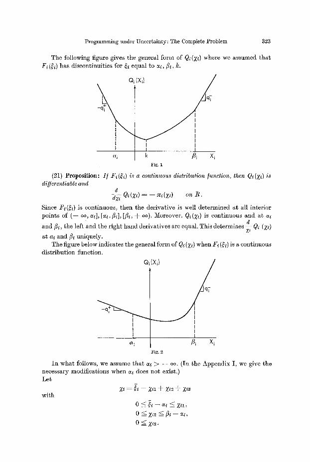
The following figure gives the general form of Q~ (Zl) where we assumed that Fi ($i) has discontinuities for ~i equal to ~i,/~/, k.

Q (X~) /

I I

a i k fli Xi Fig. 1

I / F i (~) is a continuous distribution/unction, then Qi (Zi) is ( 2 1 ) P r o p o s i t i o n : di~erentiable and

d dz~ Q i ( z ~ ) = - z~i(Zi) o n R .

Since Fi (~i) is continuous, then the derivative is well determined at all interior points of (-- oo, ei], [~, ill], [fii, q- oo). Moreover. Qi (Zt) is continuous and at at

and fit, the left End the right hand derivatives are equal. This determines ~ Qi (Z~)

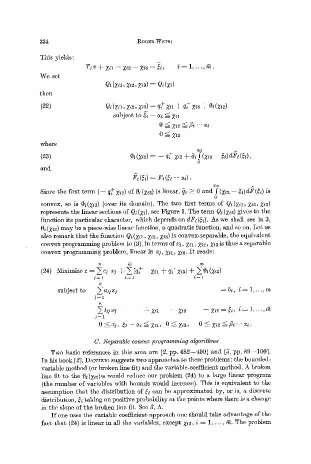
at at and fit uniquely. The figure below indicates the general form of Q~ (Z~) when Ft (~t) is a continuous

distribution function.

Qi(Xi) /

I I I I I I I

a i Bi Xi Fig. 2

In what follows, we assume that ~ / > -- oo. (In the Appendix I, we give the necessary modifications when ~ does not exist.) Let

Z~ = ~ -- Zil 4- Zi2 4- Zi3 with

0 ~__~i-- ~ti =~__ Zi l ,

0 _-< Zi . s fi~ - a~,

0 ==_ 2:~3-

324 Roo~W~Ts:

This yields:

We set

then

(22) Q~ (Z~i, Z~, X~) = q+ )/ii § q/- Xt~ § 0~ (Z~)

subject to ~ -- ~i G Z~l

0 ~ Zi~

where

(231 O~ (Zi2) = -- q+ )/~2 -]- q~ f (Z~2 -- ~) d/~ (&), 0

and

Z~2

Since the first term (-- q+ Z~21 of 0~ (Z~2) is linear, ~ _>_ 0 and ] (Zt2 -- ~)d/~(&) is 0

convex, so is 01 (g~) (over its domain). The two first terms of Q~ (Zu, Z~, Z~a) represents the linear sections of Qi (Zi), see Figure 1. The term Q~ (Zi2) gives to the function its particular character, which depends on dF~ (&). As we shall see in 3, 0~ (Z~2) may be a piece-wise linear function, a quadratic function, and so on. Let us also remark that the function Q~ (Z~l, %~u, Z~a) is convex-separable, the equivalent convex programming problem to (3), in terms of xj, Zii, Zi2, Zi~ is thus a separable convex programming problem, linear in x~-, Z~l, ~/f3- I t reads:

~ m

(24) Minimize z ---- cj xj + ~ [q+ Zu + q~- Zi3] + ~ 0/(Z~2) j = l i = 1 i = 1

subject to ~ a~jxj : b~, i = 1 , . . . ,m ] = 1

j = l

0 = xj., ~ - - ~ _-< X~i, 0 ~ Xi3, 0 = Zi2 =< fi~ - - ~ i .

C. Separable convex programming algorithms

Two basic references in this area are [2, pp. 482--490] and [5, pp. 89--100]. In his book [2], DAy,zIG suggests two approaches to these problems : the bounded- variable method (or broken line fit) and the variable-coefficient method. A broken line fit to the 0i (Z~2)'s would reduce our problem (24) to a large linear program (the number of variables with bounds would increase). This is equivalent to the assumption that the distribution of ~ can be approximated by, or is, a discrete distribution, ~.~ taking on positive probability at the points where there is a change in the slope of the broken line fit. See 3, A.

I f one uses the variable coefficient approach one should take advantage of the fact tha t (24) is linear in all the variables, except Zi2, i = 1 . . . . . ~ . The problem


then becomes: n

(25) Minimize z = ~ c~xl ~- ~. [q+ i = 1 i = 1

subject to ~a~x~ ~'=:

%

m

i = 1

and

bi, i = 1 , . . . , m

-~-Z~: --Zia - - Z ~ : $ ~ , i : l . . . . .

0 < x~, & - - ~ < ~/~, 0 < ~ , 0 < 9~ < fl~ - - ~ ,

~t~ > O, g~ > O~ (l~) + = = = - q ~ ,~ + ~ ~ , , ~ - ~ , d~ ~ , . ~ , , 0

i = l . . . . . ~ .

The solution me thod to this class of problems as well as the convergence propert ies are fully discussed in [2, pp. 486--490, pp. 433--438].

3. The probability space: (Z, ~', F)

I n this section we derive the equivalent convex p rogramming problem to (3), for some specific dis t r ibut ion functions F. Up to now, the assumpt ion made on the dis t r ibut ion of ~ /were l imited to : E (~/} exists and one can compute the value of Zi2

(Z~2 - - ~i)dFi(~i), VZi2 G [0, fli - - ~ ] ff gl > - - 0% (more general ly one can 0

gt

in tegra te ] ($i - - zi)dF~(~i), VZ~ G [ ~ , fi~] i.e. the formulas of the Rieman-

Stieltjes in tegra t ion b y par t s apply). We did not require the independence of the ~i.

A. ~ is finite

The nota t ions used in this pa rag raph differ sl ightly f rom the previous section. Le t ~ < ~ , . . . , < ~.'~ be the values assumed by ~ with probabil i t ies /1,

1~ . . . . . 17' respectively. Le t

8 - - 1

l = l

Fik,+:____ 1 : Prob {~i < oo}, Fi : 1 Prob (~l < ~ } : 0, k~

1 = 1

I t is easy to see t ha t

E~{Minq+yi ' ~ - q i - Y ~ ] ~ i ~ Z i ~ "~+~ z _ z ~ ~ & } = q~+ ~ (~ x~)/~ + q~- (x~ - ~1I~. l = s § 1=1

Then k ~ §

l = 1

326 Roo~a W~Ts :

where ~ Z~ = Z*, l = 1

l _ _ 0 < z~ < ~ - ~i -1 = d, - - 2, . . . , k~, 0 < ~ + 1

Since ~ >_ 0 (the second stage prob lem is bounded by assumption) and

F ~ < F ~ + ~ for l = l . . . . . h

i t is readily seen t h a t Q~ (Z~) is a piece-wise linear convex [unction. This last p rope r ty allows us to formulate our original problem as a linear p rogram [2, pp. 484--485], v i z . :

n ~ k~+ 1 ~,

(26) Minimize z ~ ci xY - - Z Z (q+ Fz : " j = l , = ~ , = ~ , = 1

n

subject to ~. a~ xj ---- b~, i = 1, . . . , m i = l

n ki

j = l l=l

xj_>0, j=L . . . , n z~ --< d~, o =< z~ --< 4 , o __< z , ~,+~

for i : l . . . . . m and 1 = 2 . . . . . / c r ~g

where ~ q+ ~ is a constant . i = 1

- - %~I in (24) corresponds to Z~ and Z~3 in (24) corresponds to %~ '+1. The var iables Z~, 1 = 2, ...,/c~ in (26) correspond to the unique var iable g~2 in (24).

This problem can now be solved using a linear p rogramming code with upper- bound variable option.

1. Allocation o] aircraft to routes under uncertain demand. The approach indicated above could be a t t r ibu ted to F~RGUSO~ and DANTZm where it was underlying their work: "Allocat ion of Aircraf t to Routes under Uncer ta in Demand. , , [2, pp. 568--591 ]. Using their notat ion, the problem wri t ten in s tandard fo rm (3) is:

m - - l n - - 1 n - - 1 n - - 1

i= l j= l j = l j = l n

subject to ~ x/j = a~, i = 1, . . . , m - - 1 j = l m--1

Pc" xtj + xmj - - y;' ---- ~I, j = 1 . . . . . u - - 1 i=1

x~i~O , Xmj>=O, y j ~ O , i = l , . . . , m - - 1 ; j = l , . . . , n ,

where yj is the number of seats remaining available and ~j here is their d i. The in te rpre ta t ion of the other symbols is given in [2, pp. 574]. This problem has the following features:

Cmj=O for a l l j .

Programming under Uncer~Mnty: The Complete Problem 327

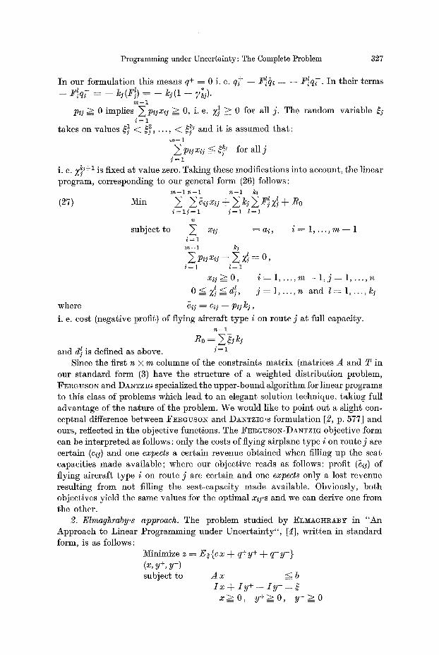
I n our formulat ion this means q+ = 0 i. e. q~' F ~ ~ - - - =- - - F~qi �9 In their terms - kj(F ) * -- F @ . . . . . 7hj)"

m--1

Pii > 0 implies ~ p,jxij > O, i. e. Z~ > 0 for all j . The random variable ~j i = 1

takes on values ~J < ~2 . . . . . < ~J and it is assumed tha t : ~7~--1

p jx,j < @ for all j ] = 1

i. e. Z~ J+l is fixed at value zero. Taking these modifications into account, the linear program, corresponding to our general form (26) follows:

m--1 n--1 n--1 k~

(27) Min Y JYP Z + R0 i = 1 ] = 1 ] = 1 / = 1

subject to ~ xo" = a i , i = l . . . . . m - - 1 i = 1 m - - 1 k~

Zj = O, i = 1 / = 1

x i j > O , i = 1 . . . . . m - - l , j = l . . . . . n

0 < Z ~ < d ~ , j = l . . . . , n and l = l . . . . . k i

where c/j = %" -- Pij kj,

i. e. cost (negative profit) of flying aircraft type i on route j at full capacity. n--1

R0 = and d~ is defined as above, j = 1

Since the first n X m columns of the constraints mat r ix (matrices A and T in our s tandard form (3) have the s tructure of a weighted distr ibution problem, F r R a u s o x and DANTZm specialized the upper-bound algori thm for linear programs to this class of problems which lead to an elegant solution technique, taking full advantage of the nature of the problem. We would like to point out a slight con- ceptual difference between F~Rauso~ and DANTZm'S formulat ion [2, p. 577] and ours, reflected in the objective functions. The F~GVSo~-DANTZm objective form can be interpreted as follows : only the costs of flying airplane type i on route j are certain (ci3") and one expects a certain revenue obtained when filling up the seat capacities made avMlable; where our objective reads as follows: profit ( ~ ) of flying aircraft type i on route j are certain and one expects only a lost revenue resulting f rom not filling the seat-capaci ty made avMlable. Obviously, bo th objectives yield the same values for the opt imal x~,s and we can derive one from the other.

2. Elmaghraby,s approach. The problem studied by ELMAGHRABY in " A n Approach to Linear Programming under Uncer ta in ty" , [4], wri t ten in s tandard form, is as follows:

Minimize z =- E~ {c x + q+ y+ + q - y - } (x, y+, y-) subject to A x < b

I x + Iy+ - - I y - =- x > 0 , y + > 0 , y - > 0

328 RoG~W~rs:

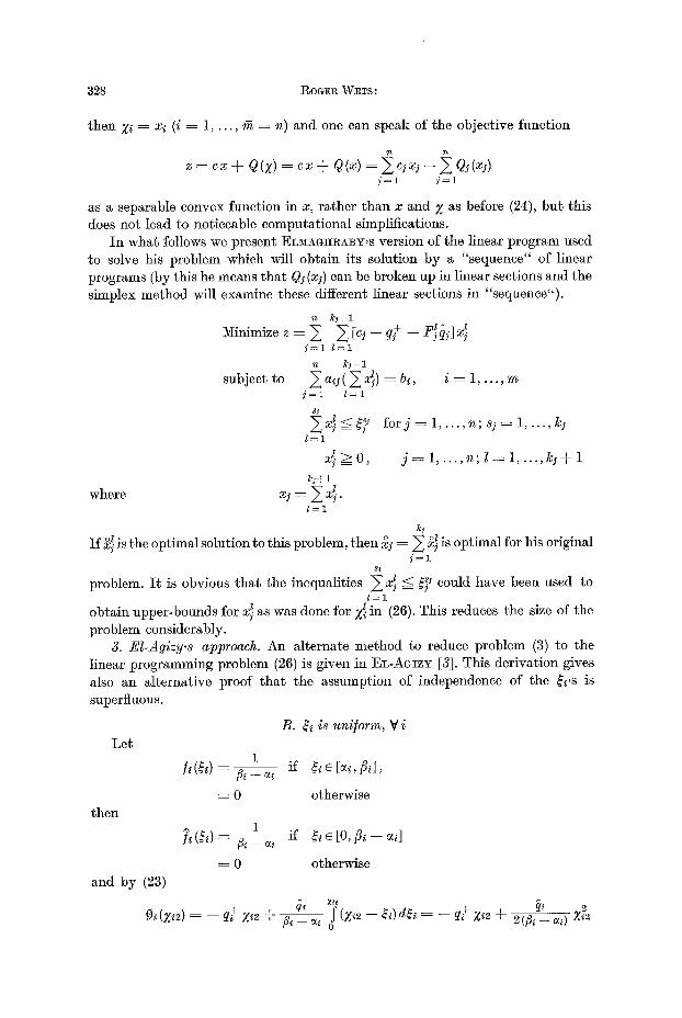
then Z~ = xi (i ---- 1 . . . . . ~ = n) and one can speak of the objective function

z = c x + Q(x) = c x + Q(x) = y c jx j + Qj(xj) 3"=1 i=1

as a separable convex function in x, rather than x and Z as before (24), but this does not lead to noticeable computational simplifications.

In what follows we present ELMAG~ABY,S version of the linear program used to solve his problem which will obtain its solution by a "sequence" of linear programs (by this he means that Qj (xj) can be broken up in linear sections and the simplex method will examine these different linear sections in "sequence").

n /c~+l

Minimize z = Z s ] = 1 l = 1

/ c i + l

subject to a/j ( ~ x}) = hi, i = 1 . . . . . m y=l 1=1

8t

Zx~ ____< ~ ' f o r j = 1 . . . . . n ; s j = 1 . . . . . /c 1 / = 1

x} >= O, j = l, . . . ,n ; l = l . . . . . !cjq-1 lcj+ l

where x;. = ~, x}. / = 1

]cj

I f }~ is the optimal solution to this problem, then ~;. = ~ ~ is optimal for his original ]=1

sj

problem. I t is obvious that the inequalities ~ x} G ~ ' could have been used to / = 1

obtain upper-bounds for x} as was done for X~ in (26). This reduces the size of the problem considerably.

3. EI-Agizy,s approach. An alternate method to reduce problem (3) to the linear programming problem (26) is given in EL-AGIzu [3]. This derivation gives also an alternative proof tha t the assumption of independence of the ~i's is superfluous.

Let

then

B. ~i is uni/orm, V i

1 / i (~i)-- fit--at if ~i~[ai ,f i i] ,

= 0 otherwise

i

----- 0 otherwise

and by (23)

r (;/~2) = - - q+ ;/42 q- /h z ~ ~ ~ (Zi2 - - &) d& = - - q+ Zi2 q- 2 ( & - - ~t) X~2


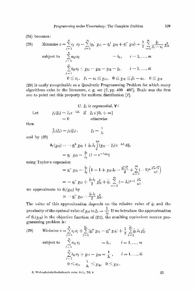
(24) becomes :

(28) Minimize z = c~ x i + (q+ Z~I - - q~ Z~2 + qi- Zta) + g N Z~ j = l / = 1 i =

%

subject to ~ at~ xl ---- be, i : 1 . . . . , m i = l

~ t # x ~ + Z i l - - Z ~ 2 - - Z i 3 : ~ { , i : 1 . . . . . ~ ] = 1

(28) is easily recognizable as a Quadratic Programming Problem for which many algorithms exist in the literature, e. g. see [2, pp. 490--491]. Beale was the first one to point out this property for uniform distribution [1].

C. ~ is exponential, u i

Let [i(&) = z~e~ -~'~' ff &e [0, + co]

----- 0 otherwise then

1

and by (23) Zr

r + 0

~ (1 - e -;~xr

using Taylor,s expansion ,2 2 oo , n ) n \

.=3 ~.v ]

~,h Z/22 ~ z~5 = - - q+ Xi2 § 2 ~ " § ~ "" ( - - )~i)n-1 n!

I t s 3

we approximate to 0i(Z/2) by

The value of this approximation depends on the relative value of {{ and the 1

proximity of the optimal value of ZiP to ~{ : ~ - I f we introduce the approximation

of G: (X{2) in the objective function of (24), the resulting equivalent convex programming problem is:

n Yn l ~-n_

(29) Minimize z = ~ c 3 x;. § Z [q+ Zil -- q+ Z{~] § ~ Z q * 2, Zi~.2 j= l i=I =

subject to ~ a{j x~ = b{, i : 1 . . . . . m ] = 1

n ]

Qyxy § z l l - - Z i P - - - - i = l , . . . , y=l ;ti '

1 0 G x ~ , X~ G; /~ , 0 G ; / ~ .

Z. Wahrscheinlichkei~stheorie verw. Geb., Bd. 4 23

330 ROGER WETS:

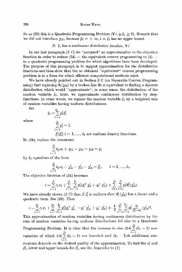
So as (28) this is a Quadratic Programming Problem (Vi, ql).i ~ 0). Remark tha t we did not introduce Z,a, because fii = + c~, i. e. ~, has no upper bound.

D. & has a continuous distribution/unction, V i

In our last paragraph (3. C) we "accepted" an approximation to the objective function in order to reduce (24) - - the equivalent convex programming to (3) - - to a quadratic programming problem for which algorithms have been developed. The purpose of this paragraph is to suggest approximation for the distribution functions and then show tha t the so obtained "equivalent" convex programming problem is in a form for which efficient computational methods exist.

We have already pointed out in Section 2. C (on Separable Convex Program- ming) tha t replacing 0~ (%*~) by a broken line fit is equivalent to finding a discrete distribution which would "approximate", in some sense, the distribution of the random variable $~. Here, we approximate continuous distribution by step- functions. In other words, we replace the random variable & by a weighted sum of random variables having uniform distributions.

Set ~,

where ~,

1=1

1~ (~) 1 = 1 . . . . . k~ are unitbrm density functions.

In (24), replace the constraint

n ~ t~jxj + g i l - Xi~ - Z~a = ~

i = l

by k, equations of the form

i l l l l t~j xj + Za - - %i2 - - Zia = &, j = l

The objective function of (24) becomes

n r~ /r

1 = 1 , . . . , k , .

j = l i = 1 / = 1 i = 1 1 = 1

We have already shown (8. C) tha t if ~{ is uniform then 0{ (Z~2) has a linear and a quadratic term. See (28). Then

j=l i=I/=i ii

This approximation of random variables having continuous distribution by the sum of random variables having uniform distributions led also to a Quadratic

Programming Problem. I t is clear that the increase in size ( 3 r ~ (/c~ -- 1) new }-n i = 1

variables of which 2 ~ . ( / ~ - 1) are bounded and ( / c i - 1 )~ additional con- i = 1

straints) depends on the desired quality of the approximation. To find the ~.~ and /~, lower and upper bounds for $~, see the Appendix to [1].


E. Summary

This section has shown tha t either directly or by approximation it was some- times possible to reduce the equivalent convex programming to (3), to program- ruing problems for which we possess efficient algorithms. For simplicity we have assumed in each paragraph tha t the marginal density func t ion / i ($i) was of the same nature V i. This is not Ilecessarily the case. I t should be clear by now tha t each 0~ (Zi2) can be treated independently. For instance, if ~1 has a discrete distribution, and say ~2 a uniform distribution it is not difficult to show tha t the equivalent convex programming problem is a quadratic programming problem.

4. An algorithm for continuous distribution functions

We now give an algorithm to solve problem (3) when V~,/~i ($i) is a continuous distribution function. We assume tha t the distribution functions F~(~) allow Rieman-Stieltjes integration of linear functions of $i. We also assume tha t (3) is solvable which implies among other conditions tha t q ~ 0. We have shown (4) tha t the equivalent convex programming to (3) can be written

(30) Minimize z(x) = cx + Q(x)

subject to A x = b

x > 0 o r

(30')

where

then

Minimize z (x, Z) = c x -}- Q (Z)

~ X ~ b

T x - - Z = 0

x=>0

m

i = 1 i = 1

Q (x) = ~ q~+ ~i - ~ [~i (T~ x) + =~ (T~ x) T~ z]. i = 1 i = l

Since ~. q~+ ~l is a constant, we may delete this term from the objective function i = l

m

of our problems. We also write ~o(Z ) = ~ ~v~ (Zi). i = 1

Problem (30) becomes n 4h

(31) Minimize ~ (x) = ~ c j x j -- ~ [~fi(Tix) + ~ ( T i x ) Tix] ] = 1 i = 1

subject to ~ aiix j = b, i = 1, . . . , m j= l xj >= 0, j = 1, . . . , n

We should note tha t : I f F/(~i) is continuous at ~ = Zi, then

23*

332 Ro~v,~ W~s:

(36) that [c - - ~ (Z) T] x ~ [c - - ~ (Z) T] ~.

I f F~ (~i) has a non-zero j ump a t ~i = Z~ then

and

In this case a complete range of values exist for the expected values of opt imal solutions to (14). Ident ica l relat ions hold for ~ (Zi). I n wha t follows, we assume t h a t f~ (~l) is a continuous distr ibution, V i = 1 . . . . . N. The following proposit ions enable us to derive an a lgor i thm to solve problem (31), and consequent ly prob lem (3).

(32) Proposition: d x ( x ) = c - - z ( 2 ) T ( i . e . S x j - - c~ - - [z(Z ) T]t). d

The result is immedia te if we r emark t h a t (21) yields ~/~- Q(Z) = - ~ (Z)

and also t h a t g = T x .

(33) Proposition: [c - - u ( Z ) T ] x - - yJ(~) is a suppor t ing hyperplane o / ; ( x ) at x ~ 2 where g = T 2 .

I n view of (32), i t suffices to show t h a t ; (2) = [c - - ~ (Z)T] 2 - - ~ (Z) which is obvious by the definitions of ; (x).

(34) Proposition: I / 2 ~ K and [c - ~(2) T] (x - - 2) ~ 0, V x ~ K then ~ (x) has a m i n i m u m at ~.

Since ; (x) is convex, then the following inequal i ty holds [7] :

~ ( x ) - ~(~) _> [c - ~ ( ~ ) T ] ( x - ~).

Moreover, b y hypothesis the second t e rm of this inequal i ty is non-negat ive for all x ~ K. This implies

; ( x ) ~ ; ( 2 ) , V x c K .

(35) Proposition: Let x, ~ ~ K and such that [ c - ~ ( Z ) T ] x > [ c - ~ ( z ) T ] 2 then ~ x ~ ~ (x, ~] such that ~ (x ~ ~ ~ (x).

Since [c - - ~ (Z) T] x > [c - - 7r (Z) T] ~, we have

[c - ~ (z) T] x > [c - - z (Z) T] (;~ x + (1 - - ~) ~) , V )~ c [0, 1).

I f ~ (x) ~ ~(~x ~- (1 - - 2~)2) V)~ e [O, 1], consider

~ ( ~ ) = ~ ( ~ x ~ - ( 1 - - 2 ) ~ ) where ~ e [ O , l ] .

Since z (x) is differentiable, so is ~ (~) [6]. Then

d

This implies t h a t ~ ~0 e [0, 1) such t h a t

~(~0) < ~(1) . Let

x ~ ---- ~0x -~ (1 - - ~0)~ we have ~(x ~ ~ ~(x) which contradicts

~(x) g ~ ( ) ~ x ~ - ( 1 - - ~ ) 2 ) , u

Proposition: Let x ~ K and ~(x) ~ ~(x ~ -~ Minimum ~(x), then ~ 2 such x e K

Programming under UncertMnfy: The Complete Problem 333

Since ; (x) is convex and b y our hypothesis we have

0 > ; (x ~ - - ; (x) ~ [c - - ~ (Z) T] (x ~ - - x) .

This Iast two proposit ions suggest an i tera t ive procedure, the nex t proposi t ion gives us a tes t of opt imal i ty .

(3'7) Proposit ion: ; ( x ~ -----Minimum ~(x) i / and only i / X~K

[c - - 7~ (X ~ T] x ~ = Min immn [c - - x~ (X ~ T] x where X ~ ~ T x ~ . x ~ K

Let [ c - - ~ ( z 0 ) T ] x ~ g [ c - - z ( z ~ V x e K then b y (34) x o is optima]. Le t ~(x ~ g ~(x), V x e K and asume t h a t ~x ~ K such t h a t

[c - - ~ (Z ~ T] x ~ > [c - - ~ (Z ~ T] x

then b y proposi t ion (35), ~ 2 e (x ~ x] such t h a t ~ (2) < ~ (x0), which contradicts the assumpt ion : ~x e K such t h a t [c - - ~(Z ~ T J x o > [c - - ~ ( Z ~ T]x .

Let us now consider the following l inear p rogramming problem.

(38) Minimize [c - - u (Z ~) T] 2

subject to A 2 ---- b

2 > O

X ~ ~ T x k , x ~ ~ K .

Since p rob lem (31) is solvable, so is problem (38) Vx ~ e K ; (proposition (20) and the l inear i ty of the t e rm cx proves the cont inui ty of ~ (x) over K). B y (37), if x ~ is an op t imal solution to (38), t hen x ~ is op t imal for (31). I f x ~ is not an opt imal solution, then b y (36) the opt imal solution to (38), say ~ , is such t ha t

[c - ~ (Z ~) TJ (x~ - ~ ) > 0

then b y (35), 3 x k+l e (x ~, ~k] such t h a t

;(x~+t) < ~(z~).

Since x ~+1 e K, we can find ~ (Z ~+1) and solve a new linear p rog ram of the fo rm (38) where we introduce the new values for the row vector ~ (Z). To find x ~+1 consider the fnnct ion:

(39) ~(2) = ~(Px~ + (i - - 2)2k), 2 e [0, 1] n n

i = 1 j = l i ~ 1

i = 1

Since z (x) is differentiable, so is ~ (2) [6]. The der ivat ive of ~ (2) wi th respect to 2 for 2s --< 2 --< ~s+l, is

(~0) ~ - - ~ ( 2 ) = c ( ~ ~ ) - ~q~+ (z~ -~ ~ - - z ~ ) + ~ q~(z~ - z~) ~ dF~(&) d)~

i e lSa

where

334 ROOEB WETS:

where

and

and

I~ = {i

= {i - -

{As) = {0,

ks < As+~

Z~ -- Z~ l

~ - ~ < AsK z~ - ~ = J

1, z~ Z~ ' Z~"~ -- ~~z~ ' i = 1 . . . . , r ~ / ~ [0, 1]

, V s = {1,2 . . . . . r = < 2 ~ + 2 } .

We assumed here t ha t Z~ - - Z~ > 0, this is not the case Vi, we develop the

der ivat ion of j z ~ (4) in more detail in Appendix I I . To find the m i n i m u m of

d (4) we successively compute the value o f ~ - ~ (4) a t the points ks (at mos t 2 ~ - ~ 2,)

for s---- 1, . . . , r.

I f d-- ~ ~(0) >= 0 then ~(A) a t ta ins its m i n i m u m on [0, 1] a t A ---- 0.

I f ~ (ks) _--< 0 and ~ ~ (2s+1) => 0 then ~ (A) a t ta ins its m i n i m u m a t some

A e [A~, As+l].

I f d ~ ( 1 ) =< 0 then ~(A) a t ta ins i t s m in imum on [0, 1] a t A = 1.

I f ~ (4) a t ta ins its m i n i m u m a t A ---- 1, then

(x~) = ; (x ) , V x e [x~, ~k].

This implies t h a t x ~ was an op t imal solution to (38), otherwise we contradic t (36), thus x ~ is an opt imal solution to (31). Le t A ~ be the m i n i m u m of$(A) = ~(Ax ~ + (1 - - A)2 ~) on [0, 1), we set

x ~+1 = A~x ~ + (1 - - A~)2 ~.

A flow char t of this a lgor i thm is given a t the end. We now show the convergence of this process. Proposi t ions (35) and (36) assure us t h a t if x ~ is not an op t imal solution for (31), then z (x ~) > z(x ~+1) since z(x) a t ta ins its m i n i m u m value on [x ~, 2 ~] a t x~+L Moreover, p rob lem (31) being solvable implies t h a t the series {z (x~)} is Cauchy convergent .

(41) Proposit ion: [c - - z ( z ~ ) T ] ( ~ - - x ~) <= z ( x ~ - - z ( x ~) where x ~ is an

opt imal solution o/ (31). Since ~ (x) is convex and b y (21)

(x ~ - - ~ (x ~) ~ Iv - - zv (Z ~) T] (x ~ - - x~)

and since 2~ is opt imal for (38), we have

[c -- ~ (g ~) T] x ~ => [c -- ~ (g ~) T] ~ .

Adding up these two inequalities gives the desired result. F r o m this last proposit ion, we have obta ined a lower bound for ~ (x ~ and

(42) ~ (x~) -t- [c - - ~ (Z k) T] (2~ - - x~) =< ; (x 0) =< ~ (x~).


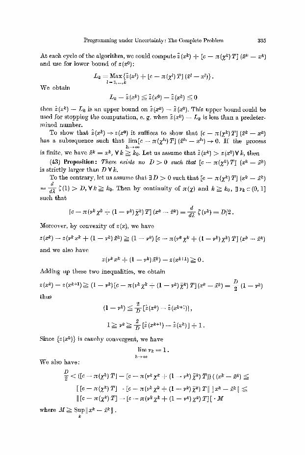
At each cycle of the a lgori thm, we could compute ~ (x k) § [c - - 7~ ( i f ) T] (2~ - - x ~) and use for lower bound of z (x ~ :

L~ = Max{~ (x~) + [c - - z(Zz) T] (~z _ x~)}. l = 1 ..... k

We obtain

L~ - - ~ (x ~) ~ ~ (x o) - - ~ (x ~) =< 0

then ~ (x k) - - L~ is an upper bound on ~ (x k) - - ~ (xO). This upper bound could be used for s topping the computa t ion , e. g. when ~ (x ~) - - Lk is less t han a predeter- mined number .

To show t h a t ~ (x ~) --> z (x ~ i t suffices to show t h a t [c - - z ( i f ) T] ( ~ - - x ~) has a subsequence such t h a t l i m [ c - 7~(Z k~) T] ( 2 k ~ xk,)__> O. I f the process

is finite, we have ~ ~-- x ~, V k ~ k0. Le t us assume t h a t ~ (x~) > z (x ~ V k, then

(43) Proposit ion: There exists no D > 0 such that [c - - ~:(Z k) T] (x ~ - - 2 ~) is s t r ict ly larger t han D V k.

To the contrary , let us assume t h a t 3 D > 0 such t h a t [c - - ~(Z ~) T] (x ~ - - 2 ~) d

- - d~ ~(1) > D, Vk _>__/Co. Then b y cont inui ty of ~(Z) and /C ~ /Co, 3vk ~ (0, 1]

such t h a t

d [c - - ~(v~Z ~ § (1 - - v~) ~k) T] (x ~ - - ~k) = ~ - $(v ~) = D/2 .

Moreover, b y convexi ty of z (x), we have

z(x~) - z(~,~x~ § (1 - ~) ~ ) => (1 - ~ ) [c - z ( ~ X ~ + (1 - ~ ) ;r T ] (x~ - - ~ )

and we also have

z(~,~x ~ § (1 - - ~ ) ~ ) - - z (x ~+~) ~= O.

Adding up these two inequalities, we obta in

D z (x ~) - - z(x ~+1) ~ (1 - - ~ ) [c - - 7~(f~Z ~ § (1 - - f~) ]~) T] (x/c - - 2 ~) = -2- (1 - - v~)

thus 2 .

(1 - ~) =< ~ [ z (x~ ) - ~ ( x ~ + ~ ) ] ,

l__~ ~ k ~ ~---Vz(x k + l ) - z ( x ~)] § 1 .

Since {z (x~)} is cauchy convergent , we have

l im v~ = 1. ~----> oo

We also have :

D < ([c - ~(Z~) T] -- [c -- ~(~Z ~ + (I -- ~) ~) T]) ( (x~ -- ~) _<

]1 [c - - 7~(ff) T] - - [c - - ~(v~X ~ § (1 - - ~ ) ~ ) T[] [Ix ~ - - ~ [ !

iI [c - - = ( i f ) T] - - [c - - x ( ~ Z ~ § (1 - - ~)Z~) T] ][. M

where M ~ Sup II x~ - ~ Jl. k

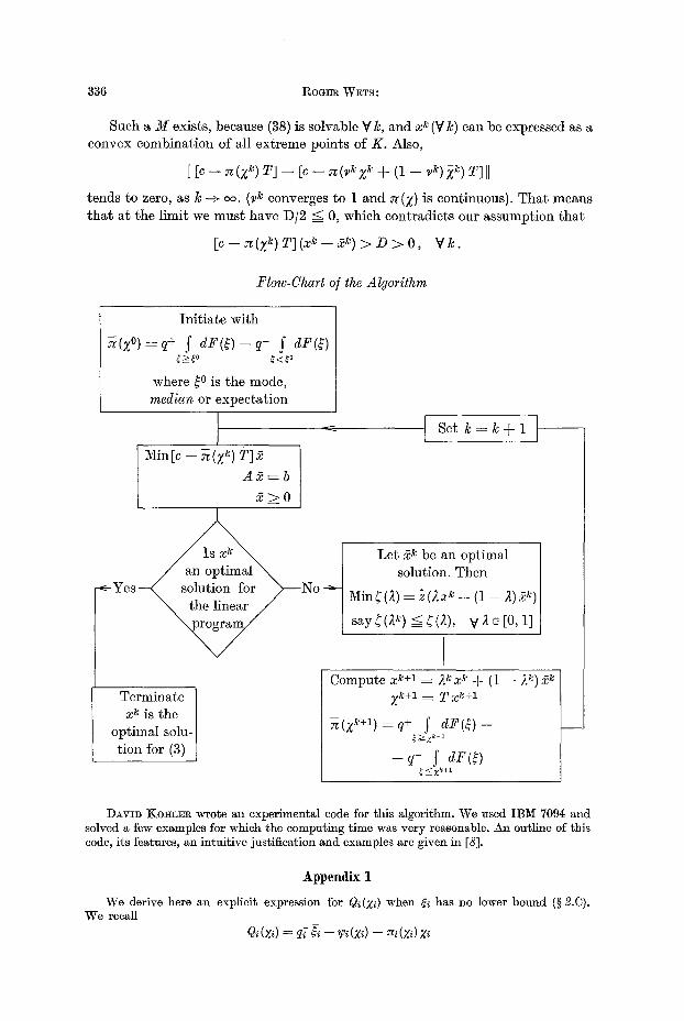
336 ROoERWETs:

Such a M exists, because (38) is solvable Vk, and xk(Yk) can be expressed as a convex combination of all extreme points of K. Also,

l] [c -- x(Z k) T] -- [c -- 7~(v~ Z~ ~- (I -- ~) ~k) T] [I

tends to zero, as/~ -+ oo. (v/~ converges to 1 and ~ (Z) is continuous). That means that at the limit we must have D/2 --< 0, which contradicts our assumption that

[c - ~(Z ~) T] (x~ -- ~ ) > D > O, V k.

Flow-Chart o/the Algorithm

Initiate with

(Z ~ S d F ( ~ ) - - q - S dF(~) ~>~o ~<~o

where ~o is the mode, median or expectation

Min[c -- .~ (;g~) T]2

A 2 = b 2 > 0

-<--Yes No ~

Terminate ] x k is the /

optimal solu-] tion for (3) ]

Set k = k q - 1 [ - -

Let 2~ be an optimal solution. Then

Min~(~) ---- ~(~z~ + (1 -- ~)2k)

say~(~ k) G~()~), V ~ [ O , ] ]

Compute )C k+ l = )JC Z/c + ( l - - ~k)2/c

Z k+l = TX ~+I

~(Z k+l) =q+ ; dE(J)--

- q - f dF($)

DAVID ]:~OtlLER wrote an experimental code for this algorithm. We used I B ~ 7094 and solved a few examples for which the computing t ime was very reasonable. An outline of this code, its features, an intui t ive justification and examples are given in [8].

Appendix 1

We derive here an explicit expression for Q~(Z~) when ~ has no lower bound (w 2.C). We recall

+ Q~(z~) = qi & - w~(z~) - ~(z~) z~

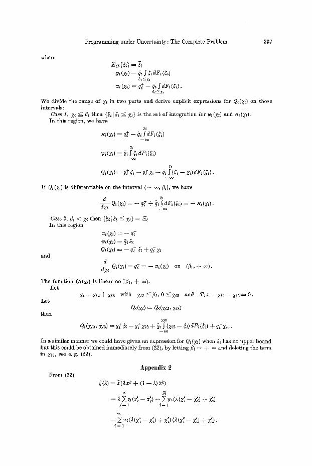
Programming under Uncer ta in ty : The Complete Problem 337

where

We divide the range of Z~ in two parts and derive explicit expressions for Q~(7,~) on those intervals:

Case 1. Z~ <= fli then {&[ ~ G %~} is the set of integrat ion for Y~i(g~) and ~(Z~). In this region, we have

Z~

~*(z*) = q+ - ~i J" dFd&)

Zi

Zi

- - c o

I f Q~06) is differentiable on the interval ( - - ~o, fii), we have

d z~ d% ~ Q~ (Xi) = - ~ + ~ ~ dF~ (&) = - - ~i (%i).

Case 2. fl~ < Z~ then {$~[& g Z~} = Z~ In this region

~(Z~) = -- q~

~(z~) = ~ &

Q~(Z~) = - q~ & + ~ ; /~ and

d d)/, Q~(7~) = q~ = - - ~(Z~) on (fl~, + o~).

The function Q~(y~) is l inear on [fig, q- ~) . Let

Z i = Z i 2 ~ % ~ 3 with Z~2 < f l ~ , 0 ~ % ~ a Let

then Qi(Z~)=Q~(z~2, Zt3)

and T i x - - z i 2 - - % ~ 3 = 0 .

Z~2

Q*(z*2, x~3) = q$ & - ~$ x*2 + ~, f (z ,2 - &) dE, (&) + q~ X~ . - - o o

In a similar manner we could have given an expression for Q~ (Zi) when & has no upper bound bu t this could be obtained immediately from (22), by let t ing fl, ~ -i- co and deleting the term in Z~3, see e. g. (29).

From (39) A p p e n d i x 2

r = ~(Zx~ + (1 - z)~)

n k --k k

y=l i=i

~b

- Z ~ ( ; . ( z ~ - 2~1 + z~)(~4d - ~) + x~). i = 1

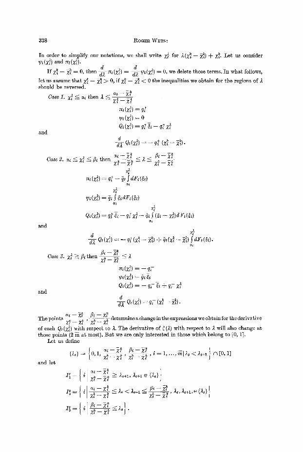
338 ROGER WETS:

I n order to s implify our no ta t ions , we shah wr i te Z} for 2(Z~ - - ~ ) + Z~. Le t us consider ~0i (J/i) a n d ~i (X~).

d ~ d I f Z} - - Z~ = O, t h e n d2 ~ (Zi) = ~ - ~i (Zi) = O, we delete those te rms. I n w h a t follows,

le t us assume t h a t Z~ - - Z~ > O, if Z~ - - Z~ < 0 the inequal i t ies we o b t a i n for t he regions of ,~ should be reversed.

Case 1. Zl < cq t h e n 2 < ei - - Z/~ = = z,~ - ~,~

~ ( z ~ ) = o

Q~(z~) = ~ , - q~z~ and

d - - ( Z ~ - - Zd

Case 2. ai ~ Z~ ~_ fl~ t h e n ~ - ~ < 2 < fli - - Z~ z ' ~ - ~.'~ = = ~ - ~

~ (z~) = q; - ~ ~ d ~ ( ~ ) otl

). + - + ).

d ,~ + q~ (;/i q~(zi - - Zi) d2 Q ~ ( Z ' ) = - - - Z ~ ) - t - - ~ -'~ Yd3"~(~d.

a n d

a n d

- - ; r < 2 Case 3. Z~ >= fit t h e n fli ~'~

~ i ( z h = - q~-

Q ~ ( z } ) = - q , - ~ + ~ , - z , ~

d

{2s} =

a n d le t

The po in t s Z~ - - Z~ ' ~Z~ ---- ~'~z~ de te rmine a change in t he expressions we o b t a i n for the de r iva t ive

of each Qi(z~) w i th respec t to 2. The de r iva t ive of ~(Z) w i th respec t to 2 will also change a t those po in t s (2 m a t most) . B u t we are only in te res t ed in those which belong to [0, 1].

L e t us define

0 , 1 , ~ - - , �9 - k i = 1 , . . . , N I 2 ~ < 2 ~ + 1 r ~ [ 0 , 1 ] z~ - 2'~

_>- i ,+1 .2 ,+1 e {~,} Zl - - Z~

- - Z i < 2 s . z g = i z~ z ~ =


If i ~ I s , that means that on the interval [As, As+L] the derivative of Q~(Z~) takes on the value

q+ (Z~ -- -l~Zi); if i e I~ we have to use the third form of the derivative of ~ Q~ (g~'). For

~ [As, )~s+l] we get: ?&

- - z ~ )

d)L i = 1 ie I~ i~ISs

A simple algebraic manipulation gives us (40). I t is very easy to see how the construction of the sets I~, I s and I.~ have to be modified if Z~ -- Z~ < 0.

References

[1] B~ALE, E. ~ . : The use of quadratic programming in stochastic linear programming. RAND P--2404, August 1961.

[2] DA~-TZIG, G. B. : Linear programming and extensions. Princeton: Princeton Univ. Press 1963.

[3] EL-AGIZY, M. : Programming under uncertainty with discrete distribution function. Univ. of California, Operations Res. Center, 0RC 64--13, 1964.

[4] EL~AOm~XBY, S. E. : An approach to linear programming under uncertainty. Operations Res. 7, No. 1, 208--216 (1959).

[5] MILLE~, C. E. : The simplex method for local separable programming. In Recent advances in mathematical programming, pp. 89--100 (Ed. Graves and Wolfe) 1963.

[6] DIEUDO:~-E]~, J.: Foundations of modern analysis. New York: Academic Press 1963. [7] ZOUTEiNDIJK, Cx. : Methods of feasible directions. Amsterdam: Elsevier 1960. [8] K6n~E~, D., and R. WETs: Programming under uncertainty: An experimental code for

the complete problem. Univ. of California, Berkeley ORC 64--15, 1964.

Mathematics Research Laboratory Boeing Scientific Research Laboratories

POB 3981, Seattle Washington 98124/USA

Documents

Programming under uncertainty: The complete problem