Embed Size (px)
Citation preview
Programming Languages:Theory and Practice
(WORKING DRAFT OF SEPTEMBER 19, 2005.)
Robert HarperCarnegie Mellon University
Spring Semester, 2005

Copyright c© 2005. All Rights Reserved.
Preface
This is a collection of lecture notes for Computer Science 15–312 Program-ming Languages. This course has been taught by the author in the Spring of1999 and 2000 at Carnegie Mellon University, and by Andrew Appel in theFall of 1999, 2000, and 2001 at Princeton University. I am grateful to An-drew for his advice and suggestions, and to our students at both CarnegieMellon and Princeton whose enthusiasm (and patience!) was instrumentalin helping to create the course and this text.
What follows is a working draft of a planned book that seeks to strikea careful balance between developing the theoretical foundations of pro-gramming languages and explaining the pragmatic issues involved in theirdesign and implementation. Many considerations come into play in the de-sign of a programming language. I seek here to demonstrate the central roleof type theory and operational semantics in helping to define a languageand to understand its properties.
Comments and suggestions are most welcome. Enjoy!

iv
WORKING DRAFT SEPTEMBER 19, 2005
Contents
Preface iii
I Preliminaries 1
1 Inductive Definitions 31.1 Relations and Judgements . . . . . . . . . . . . . . . . . . . . 31.2 Rules and Derivations . . . . . . . . . . . . . . . . . . . . . . 41.3 Examples of Inductive Definitions . . . . . . . . . . . . . . . 51.4 Rule Induction . . . . . . . . . . . . . . . . . . . . . . . . . . . 61.5 Iterated and Simultaneous Inductive Definitions . . . . . . . 71.6 Examples of Rule Induction . . . . . . . . . . . . . . . . . . . 71.7 Admissible and Derivable Rules . . . . . . . . . . . . . . . . 81.8 Defining Functions by Rules . . . . . . . . . . . . . . . . . . . 101.9 Foundations . . . . . . . . . . . . . . . . . . . . . . . . . . . . 11
2 Transition Systems 132.1 Transition Systems . . . . . . . . . . . . . . . . . . . . . . . . 132.2 Exercises . . . . . . . . . . . . . . . . . . . . . . . . . . . . . . 14
II Defining a Language 15
3 Concrete Syntax 173.1 Strings . . . . . . . . . . . . . . . . . . . . . . . . . . . . . . . 173.2 Context-Free Grammars . . . . . . . . . . . . . . . . . . . . . 183.3 Ambiguity . . . . . . . . . . . . . . . . . . . . . . . . . . . . . 193.4 Exercises . . . . . . . . . . . . . . . . . . . . . . . . . . . . . . 22
v

vi CONTENTS
4 Abstract Syntax Trees 234.1 Abstract Syntax Trees . . . . . . . . . . . . . . . . . . . . . . . 234.2 Structural Induction . . . . . . . . . . . . . . . . . . . . . . . 244.3 Parsing . . . . . . . . . . . . . . . . . . . . . . . . . . . . . . . 254.4 Exercises . . . . . . . . . . . . . . . . . . . . . . . . . . . . . . 27
5 Abstract Binding Trees 295.1 Names . . . . . . . . . . . . . . . . . . . . . . . . . . . . . . . 295.2 Abstract Syntax With Names . . . . . . . . . . . . . . . . . . 305.3 Abstract Binding Trees . . . . . . . . . . . . . . . . . . . . . . 305.4 Renaming . . . . . . . . . . . . . . . . . . . . . . . . . . . . . 315.5 Structural Induction . . . . . . . . . . . . . . . . . . . . . . . 34
6 Static Semantics 376.1 Static Semantics of Arithmetic Expressions . . . . . . . . . . 376.2 Exercises . . . . . . . . . . . . . . . . . . . . . . . . . . . . . . 38
7 Dynamic Semantics 397.1 Structured Operational Semantics . . . . . . . . . . . . . . . . 397.2 Evaluation Semantics . . . . . . . . . . . . . . . . . . . . . . . 427.3 Relating Transition and Evaluation Semantics . . . . . . . . . 437.4 Exercises . . . . . . . . . . . . . . . . . . . . . . . . . . . . . . 44
8 Relating Static and Dynamic Semantics 458.1 Preservation for Arithmetic Expressions . . . . . . . . . . . . 458.2 Progress for Arithmetic Expressions . . . . . . . . . . . . . . 468.3 Exercises . . . . . . . . . . . . . . . . . . . . . . . . . . . . . . 46
III A Functional Language 47
9 A Minimal Functional Language 499.1 Syntax . . . . . . . . . . . . . . . . . . . . . . . . . . . . . . . 49
9.1.1 Concrete Syntax . . . . . . . . . . . . . . . . . . . . . . 499.1.2 Abstract Syntax . . . . . . . . . . . . . . . . . . . . . . 50
9.2 Static Semantics . . . . . . . . . . . . . . . . . . . . . . . . . . 509.3 Properties of Typing . . . . . . . . . . . . . . . . . . . . . . . 529.4 Dynamic Semantics . . . . . . . . . . . . . . . . . . . . . . . . 549.5 Properties of the Dynamic Semantics . . . . . . . . . . . . . . 569.6 Exercises . . . . . . . . . . . . . . . . . . . . . . . . . . . . . . 57
WORKING DRAFT SEPTEMBER 19, 2005
CONTENTS vii
10 Type Safety 5910.1 Defining Type Safety . . . . . . . . . . . . . . . . . . . . . . . 5910.2 Type Safety . . . . . . . . . . . . . . . . . . . . . . . . . . . . . 6010.3 Run-Time Errors and Safety . . . . . . . . . . . . . . . . . . . 63
IV Control and Data Flow 67
11 Abstract Machines 6911.1 Control Flow . . . . . . . . . . . . . . . . . . . . . . . . . . . . 7011.2 Environments . . . . . . . . . . . . . . . . . . . . . . . . . . . 77
12 Continuations 8312.1 Informal Overview of Continuations . . . . . . . . . . . . . . 8412.2 Semantics of Continuations . . . . . . . . . . . . . . . . . . . 8712.3 Coroutines . . . . . . . . . . . . . . . . . . . . . . . . . . . . . 9112.4 Exercises . . . . . . . . . . . . . . . . . . . . . . . . . . . . . . 95
13 Exceptions 9713.1 Exercises . . . . . . . . . . . . . . . . . . . . . . . . . . . . . . 102
V Imperative Functional Programming 105
14 Mutable Storage 10714.1 References . . . . . . . . . . . . . . . . . . . . . . . . . . . . . 107
15 Monads 11315.1 A Monadic Language . . . . . . . . . . . . . . . . . . . . . . . 11415.2 Reifying Effects . . . . . . . . . . . . . . . . . . . . . . . . . . 11615.3 Exercises . . . . . . . . . . . . . . . . . . . . . . . . . . . . . . 117
VI Cost Semantics and Parallelism 119
16 Cost Semantics 12116.1 Evaluation Semantics . . . . . . . . . . . . . . . . . . . . . . . 12116.2 Relating Evaluation Semantics to Transition Semantics . . . 12216.3 Cost Semantics . . . . . . . . . . . . . . . . . . . . . . . . . . 12316.4 Relating Cost Semantics to Transition Semantics . . . . . . . 12416.5 Exercises . . . . . . . . . . . . . . . . . . . . . . . . . . . . . . 125
SEPTEMBER 19, 2005 WORKING DRAFT
viii CONTENTS
17 Implicit Parallelism 12717.1 Tuple Parallelism . . . . . . . . . . . . . . . . . . . . . . . . . 12717.2 Work and Depth . . . . . . . . . . . . . . . . . . . . . . . . . . 12917.3 Vector Parallelism . . . . . . . . . . . . . . . . . . . . . . . . . 132
18 A Parallel Abstract Machine 13718.1 A Simple Parallel Language . . . . . . . . . . . . . . . . . . . 13718.2 A Parallel Abstract Machine . . . . . . . . . . . . . . . . . . . 13918.3 Cost Semantics, Revisited . . . . . . . . . . . . . . . . . . . . 14118.4 Provable Implementations (Summary) . . . . . . . . . . . . . 142
VII Data Structures and Abstraction 145
19 Aggregate Data Structures 14719.1 Products . . . . . . . . . . . . . . . . . . . . . . . . . . . . . . 14719.2 Sums . . . . . . . . . . . . . . . . . . . . . . . . . . . . . . . . 14919.3 Recursive Types . . . . . . . . . . . . . . . . . . . . . . . . . . 150
20 Polymorphism 15320.1 A Polymorphic Language . . . . . . . . . . . . . . . . . . . . 15420.2 ML-style Type Inference . . . . . . . . . . . . . . . . . . . . . 16020.3 Parametricity . . . . . . . . . . . . . . . . . . . . . . . . . . . 161
20.3.1 Informal Discussion . . . . . . . . . . . . . . . . . . . 16220.3.2 Relational Parametricity . . . . . . . . . . . . . . . . . 165
21 Data Abstraction 17121.1 Existential Types . . . . . . . . . . . . . . . . . . . . . . . . . 172
21.1.1 Abstract Syntax . . . . . . . . . . . . . . . . . . . . . . 17221.1.2 Correspondence With ML . . . . . . . . . . . . . . . . 17221.1.3 Static Semantics . . . . . . . . . . . . . . . . . . . . . . 17421.1.4 Dynamic Semantics . . . . . . . . . . . . . . . . . . . . 17521.1.5 Safety . . . . . . . . . . . . . . . . . . . . . . . . . . . . 176
21.2 Representation Independence . . . . . . . . . . . . . . . . . . 176
VIII Lazy Evaluation 181
22 Lazy Types 18322.1 Lazy Types . . . . . . . . . . . . . . . . . . . . . . . . . . . . . 185
22.1.1 Lazy Lists in an Eager Language . . . . . . . . . . . . 187
WORKING DRAFT SEPTEMBER 19, 2005
CONTENTS ix
22.1.2 Delayed Evaluation and Lazy Data Structures . . . . 193
23 Lazy Languages 19723.0.3 Call-by-Name and Call-by-Need . . . . . . . . . . . . 19923.0.4 Strict Types in a Lazy Language . . . . . . . . . . . . 201
IX Dynamic Typing 203
24 Dynamic Typing 20524.1 Dynamic Typing . . . . . . . . . . . . . . . . . . . . . . . . . . 20724.2 Implementing Dynamic Typing . . . . . . . . . . . . . . . . . 20824.3 Dynamic Typing as Static Typing . . . . . . . . . . . . . . . . 210
25 Featherweight Java 21325.1 Abstract Syntax . . . . . . . . . . . . . . . . . . . . . . . . . . 21325.2 Static Semantics . . . . . . . . . . . . . . . . . . . . . . . . . . 21625.3 Dynamic Semantics . . . . . . . . . . . . . . . . . . . . . . . . 21825.4 Type Safety . . . . . . . . . . . . . . . . . . . . . . . . . . . . . 22025.5 Acknowledgement . . . . . . . . . . . . . . . . . . . . . . . . 221
X Subtyping and Inheritance 223
26 Subtyping 22526.1 Adding Subtyping . . . . . . . . . . . . . . . . . . . . . . . . 22526.2 Varieties of Subtyping . . . . . . . . . . . . . . . . . . . . . . 227
26.2.1 Arithmetic Subtyping . . . . . . . . . . . . . . . . . . 22726.2.2 Function Subtyping . . . . . . . . . . . . . . . . . . . 22826.2.3 Product and Record Subtyping . . . . . . . . . . . . . 23026.2.4 Reference Subtyping . . . . . . . . . . . . . . . . . . . 231
26.3 Type Checking With Subtyping . . . . . . . . . . . . . . . . . 23226.4 Implementation of Subtyping . . . . . . . . . . . . . . . . . . 234
26.4.1 Coercions . . . . . . . . . . . . . . . . . . . . . . . . . 234
27 Inheritance and Subtyping in Java 23927.1 Inheritance Mechanisms in Java . . . . . . . . . . . . . . . . . 239
27.1.1 Classes and Instances . . . . . . . . . . . . . . . . . . 23927.1.2 Subclasses . . . . . . . . . . . . . . . . . . . . . . . . . 24127.1.3 Abstract Classes and Interfaces . . . . . . . . . . . . . 242
27.2 Subtyping in Java . . . . . . . . . . . . . . . . . . . . . . . . . 244
SEPTEMBER 19, 2005 WORKING DRAFT
x CONTENTS
27.2.1 Subtyping . . . . . . . . . . . . . . . . . . . . . . . . . 24427.2.2 Subsumption . . . . . . . . . . . . . . . . . . . . . . . 24527.2.3 Dynamic Dispatch . . . . . . . . . . . . . . . . . . . . 24627.2.4 Casting . . . . . . . . . . . . . . . . . . . . . . . . . . . 247
27.3 Methodology . . . . . . . . . . . . . . . . . . . . . . . . . . . 249
XI Concurrency 251
28 Concurrent ML 253
XII Storage Management 255
29 Storage Management 25729.1 The A Machine . . . . . . . . . . . . . . . . . . . . . . . . . . . 25729.2 Garbage Collection . . . . . . . . . . . . . . . . . . . . . . . . 261
WORKING DRAFT SEPTEMBER 19, 2005

Part I
Preliminaries
1

Chapter 1
Inductive Definitions
Inductive definitions are an indispensable tool in the study of program-ming languages. In this chapter we will develop the basic framework ofinductive definitions, and give some examples of their use.
1.1 Relations and Judgements
We start with the notion of an n-place, or n-ary, relation, R, among n ≥ 1objects of interest. (A one-place relation is sometimes called a predicate, orproperty, or class.) A relation is also called a judgement form, and the asser-tion that objects x1, . . . , xn stand in the relation R, written R x1, . . . , xn orx1, . . . , xn R, is called an instance of that judgement form, or just a judgementfor short.
Many judgement forms arise in the study of programming languages.Here are a few examples, with their intended meanings:
n nat n is a natural numbert tree t is a binary treep prop p expresses a propositionp true the proposition p is trueτ type x is a typee : τ e is an expression of type τ
The descriptions in the chart above are only meant to be suggestive, andnot as precise definitions. One method for defining judgement forms suchas these is by an inductive definition in the form of a collection of rules.
3
4 1.2 Rules and Derivations
1.2 Rules and Derivations
An inductive definition of an n-ary relation R consists of a collection of infer-ence rules of the form
~x1 R · · · ~xk R~x R .
Here ~x and each ~x1 . . . ,~xk are n-tuples of objects, and R is the relation beingdefined. The judgements above the horizontal line are called the premisesof the rule, and the judgement below is called the conclusion of the rule. Ifa rule has no premises (i.e., n = 0), the rule is called an axiom; otherwise itis a proper rule.
A relation P is closed under a rule
~x1 R · · · ~xk R~x R
iff ~x P whenever ~x1 P, . . . , ~xk P. The relation P is closed under a set of suchrules iff it is closed under each rule in the set. If S is a set of rules of theabove form, then the relation, R, inductively defined by the rule set, S , is thestrongest (most restrictive) relation closed under S . This means that R isclosed under S , and that if P is also closed under S , then ~x R implies ~x P.
If R is inductively defined by a rule set SR, then ~x R holds if and only ifit has a derivation consisting of a composition of rules in SR, starting withaxioms and ending with ~x R. A derivation may be depicted as a “stack” ofrules of the form
...D1
~x1 R · · ·
...Dk
~xk R~x R
where~x1 R · · · ~xk R
~x R
is an inference rule, and each Di is a derivation of ~xi R.To show that a judgement is derivable we need only find a derivation
for it. There are two main methods for finding a derivation, called forwardchaining and backward chaining. Forward chaining starts with the axiomsand works forward towards the desired judgement, whereas backwardchaining starts with the desired judgement and works backwards towardsthe axioms.
WORKING DRAFT SEPTEMBER 19, 2005
1.3 Examples of Inductive Definitions 5
More precisely, forward chaining search maintains a set of derivablejudgements, and continually extends this set by adding to it the conclusionof any rule all of whose premises are in that set. Initially, the set is empty;the process terminates when the desired judgement occurs in the set. As-suming that all rules are considered at every stage, forward chaining willeventually find a derivation of any derivable judgement, but it is impos-sible (in general) to decide algorithmically when to stop extending the setand conclude that the desired judgement is not derivable. We may go onand on adding more judgements to the derivable set without ever achiev-ing the intended goal. It is a matter of understanding the global propertiesof the rules to determine that a given judgement is not derivable.
Forward chaining is undirected in the sense that it does not take ac-count of the end goal when deciding how to proceed at each step. Incontrast, backward chaining is goal-directed. Backward chaining searchmaintains a set of current goals, judgements whose derivations are to besought. Initially, this set consists solely of the judgement we wish to de-rive. At each stage, we remove a judgement from the goal set, and considerall rules whose conclusion is that judgement. For each such rule, we addto the goal set the premises of that rule. The process terminates when thegoal set is empty, all goals having been achieved. As with forward chain-ing, backward chaining will eventually find a derivation of any derivablejudgement, but there is no algorithmic method for determining in generalwhether the current goal is derivable. Thus we may futilely add more andmore judgements to the goal set, never reaching a point at which all goalshave been satisfied.
1.3 Examples of Inductive Definitions
Let us now consider some examples of inductive definitions. The followingset of rules, SN , constitute an inductive definition of the judgement formnat:
zero natx nat
succ(x) nat
The first rule states that zero is a natural number. The second states that ifx is a natural number, so is succ(x). Quite obviously, the judgement x natis derivable from rules SN iff x is a natural number. For example, here is a
SEPTEMBER 19, 2005 WORKING DRAFT

6 1.4 Rule Induction
derivation of the judgement succ(succ(zero)) nat:
zero natsucc(zero) nat
succ(succ(zero)) nat
The following set of rules, ST, form an inductive definition of the judge-ment form tree:
empty tree
x tree y tree
node(x, y) tree
The first states that an empty tree is a binary tree. The second states that anode with two binary trees as children is also a binary tree.
Using the rules ST, we may construct a derivation of the judgement
node(empty, node(empty, empty)) tree
as follows:
empty tree
empty tree empty tree
node(empty, empty) tree
node(empty, node(empty, empty)) tree
1.4 Rule Induction
Suppose that the relation R is inductively defined by the rule set SR. Theprinciple of rule induction is used to show ~x P, whenever ~x R. Since R is thestrongest relation closed under SR, it is enough to show that P is closedunder SR. Specifically, for every rule
~x1 R · · · ~xk R~x R
in SR, we must show ~x P under the assumptions ~x1 P, . . . , ~xk P. The as-sumptions ~x1 P, . . . , ~xk P are the inductive hypotheses, and the conclusion iscalled the inductive step, corresponding to that rule.
Rule induction is also called induction on derivations, for if ~x R holds,then there must be some derivation of it from the rules in SR. Consider thefinal rule in the derivation, whose conclusion is ~x R and whose premisesare ~x1 R, . . . , ~xk R. By induction we have ~x1 P, . . . , ~xk P, and hence to show~x P, it suffices to show that ~x1 P, . . . , ~xk P imply ~x P.
WORKING DRAFT SEPTEMBER 19, 2005

1.5 Iterated and Simultaneous Inductive Definitions 7
1.5 Iterated and Simultaneous Inductive Definitions
Inductive definitions are often iterated, meaning that one inductive defini-tion builds on top of another. For example, the following set of rules, SL,defines the predicate list, which expresses that an object is a list of naturalnumbers:
nil list
x nat y list
cons(x, y) list
Notice that the second rule makes reference to the judgement nat definedearlier.
It is also common to give a simultaneous inductive definition of severalrelations, R1, . . . , Rk, by a single set of rules, SR1,...,Rk . Each rule in the sethas the form
~x1 Ri1 · · · ~xm Rim
~x Ri
where 1 ≤ ij ≤ k for each 1 ≤ j ≤ k.The principle of rule induction for such a simultaneous inductive def-
inition gives a sufficient condition for a family P1, . . . , Pk of relations suchthat ~x Pi whenever ~x Ri, for each 1 ≤ i ≤ k. To show this, it is sufficient toshow for each rule
~x1 Ri1 · · · ~xm Rim
~x Ri
if ~x1 Pi1 , . . . , ~xm Rim , then ~x Ri.For example, consider the rule set, Seo, which forms a simultaneous
inductive definition of the judgement forms x even, stating that x is an evennatural number, and x odd, stating that x is an odd natural number.
zero evenx odd
succ(x) even
x evensucc(x) odd
These rules must be interpreted as a simultaneous inductive definition be-cause the definition of each judgement form refers to the other.
1.6 Examples of Rule Induction
Consider the rule set SN defined earlier. The principle of rule induction forSN states that to show x P whenever x nat, it is enough to show
SEPTEMBER 19, 2005 WORKING DRAFT
8 1.7 Admissible and Derivable Rules
1. zero P;
2. if y P, then succ(y) P.
This is just the familiar principal of mathematical induction.The principle of rule induction for ST states that if we are to show that
x P whenever x tree, it is enough to show
1. empty P;
2. if x1 P and x2 P, then node(x1, x2) P.
This is sometimes called the principle of tree induction.The principle of rule induction naturally extends to simultaneous in-
ductive definitions as well. For example, the rule induction principle cor-responding to the rule set Seo states that if we are to show x P wheneverx even, and x Q whenever x odd, it is enough to show
1. zero P;
2. if x P, then succ(x) Q;
3. if x Q, then succ(x) P.
These proof obligations are derived in the evident manner from the rulesin Seo.
1.7 Admissible and Derivable Rules
Let SR be an inductive definition of the relation R. There are two senses inwhich a rule
~x1 R · · · ~xk R~x R
may be thought of as being “valid” for SR: it can be either derivable or ad-missible.
A rule is said to be derivable iff there is a derivation of its conclusion fromits premises. This means that there is a composition of rules starting withthe premises and ending with the conclusion. For example, the followingrule is derivable in SN :
x natsucc(succ(succ(x))) nat.
WORKING DRAFT SEPTEMBER 19, 2005
1.7 Admissible and Derivable Rules 9
Its derivation is as follows:
x natsucc(x) nat
succ(succ(x)) nat
succ(succ(succ(x))) nat.
A rule is said to be admissible iff its conclusion is derivable from nopremises whenever its premises are derivable from no premises. For ex-ample, the following rule is admissible in SN :
succ(x) natx nat .
First, note that this rule is not derivable for any choice of x. For if x is zero,then the only rule that applies has no premises, and if x is succ(y) for somey, then the only rule that applies has as premise y nat, rather than x nat.However, this rule is admissible! We may prove this by induction on thederivation of the premise of the rule. For if succ(x) nat is derivable fromno premises, it can only be by second rule, which means that x nat is alsoderivable, as required. (This example shows that not every admissible ruleis derivable.)
The distinction between admissible and derivable rules can be hard tograsp at first. One way to gain intuition is to note that if a rule is derivablein a rule set S , then it remains derivable in any rule set S ′ ⊇ S . This isbecause the derivation of that rule depends only on what rules are avail-able, and is not sensitive to whether any other rules are also available. Incontrast a rule can be admissible in S , but inadmissible in some extensionS ′ ⊇ S ! For example, suppose that we add to SN the rule
succ(junk) nat.
Now it is no longer the case that the rule
succ(x) natx nat .
is admissible, for if the premise were derived using the additional rule,there is no derivation of junk nat, as would be required for this rule to beadmissible.
Since admissibility is sensitive to which rules are absent, as well as towhich are present, a proof of admissibility of a non-derivable rule must, at
SEPTEMBER 19, 2005 WORKING DRAFT
10 1.8 Defining Functions by Rules
bottom, involve a use of rule induction. A proof by rule induction containsa case for each rule in the given set, and so it is immediately obvious thatthe argument is not stable under an expansion of this set with an additionalrule. The proof must be reconsidered, taking account of the additional rule,and there is no guarantee that the proof can be extended to cover the newcase (as the preceding example illustrates).
1.8 Defining Functions by Rules
A common use of inductive definitions is to define inductively its graph,a relation, which we then prove is a function. For example, one way todefine the addition function on natural numbers is to define inductivelythe relation A (m, n, p), with the intended meaning that p is the sum of mand n, as follows:
m natA (m, zero, m)
A (m, n, p)A (m, succ(n), succ(p))
We then must show that p is uniquely determined as a function of m and n.That is, we show that if m nat and n nat, then there exists a unique p suchthat A (m, n, p) by rule induction on the rules defining the natural numbers.
1. From m nat and zero nat, show that there exists a unique p such thatA (m, n, p). Taking p to be m, it is easy to see that A (m, n, p).
2. From m nat and succ(n) nat and the assumption that there exists aunique p such that A (m, n, p), we are to show that there exists aunique q such that A (m, succ(n), q). Taking q = succ(p) does thejob.
Given this, we are entitled to write A (m, n, p) as the equation m + n = p.Often the rule format for defining functions illustrated above can be a
bit unwieldy. In practice we often present such rules in the more conve-nient form of recursion equations. For example, the addition function maybe defined by the following recursion equations:
m + zero =df mm + succ(n) =df succ(m + n)
These equations clearly define a relation, namely the three-place relationgiven above, but we must prove that they constitute an implicit definitionof a function.
WORKING DRAFT SEPTEMBER 19, 2005
1.9 Foundations 11
1.9 Foundations
We have left unspecified just what sorts of objects may occur in judgementsand rules. For example, the inductive definition of binary trees makes useof empty and node(−,−) without saying precisely just what are these ob-jects. This is a matter of foundations that we will only touch on brieflyhere.
One point of view is to simply take as given that the constructions wehave mentioned so far are intuitively acceptable, and require no further jus-tification or explanation. Generally, we may permit any form of “finitary”construction, whereby finite entities are built up from other such finite en-tities by finitely executable processes in some intuitive sense. This is theattitude that we shall adopt in the sequel. We will simply assume with-out further comment that the constructions we describe are self-evidentlymeaningful, and do not require further justification.
Another point of view is to work within some other widely acceptedfoundation, such as set theory. While this leads to a mathematically sat-isfactory account, it ignores the very real question of whether and howour constructions can be justified on computational grounds (and defersthe foundational questions to questions about set existence). After all, thestudy of programming languages is all about things we can implement ona machine! Conventional set theory makes it difficult to discuss such mat-ters. A standard halfway point is to insist that all work take place in theuniverse of hereditarily finite sets, which are finite sets whose elemets are fi-nite sets whose elements are finite sets . . . . Any construction that can becarried out in this universe is taken as meaningful, and tacitly assumed tobe effectively executable on a machine.
A more concrete, but technically awkward, approach is to admit onlythe natural numbers as finitary objects — any other object of interest mustbe encoded as a natural number using the technique of Godel numbering,which establishes a bijection between a set X of finitary objects and the setN of natural numbers. Via such an encoding every object of interest is anatural number!
In practice one would never implement such a representation in a com-puter program, but rather work directly with a more natural representationsuch as Lisp s-expressions, or ML concrete data types. This amounts to tak-ing the universe of objects to be the collection of well-founded, finitely branch-ing trees. These may be encoded as natural numbers, or hereditarily finitewell-founded sets, or taken as intuitively meaningful and not in need offurther justification. More radically, one may even dispense with the well-
SEPTEMBER 19, 2005 WORKING DRAFT

12 1.9 Foundations
foundedness requirement, and consider infinite, finitely branching trees asthe universe of objects. With more difficulty these may also be representedas natural numbers, or, more naturally, as non-well-founded sets, or evenaccepted as intuitively meaningful without further justification.
WORKING DRAFT SEPTEMBER 19, 2005
Chapter 2
Transition Systems
Transition systems are used to describe the execution behavior of programsby defining an abstract computing device with a set, S, of states that arerelated by a transition relation, 7→. The transition relation describes how thestate of the machine evolves during execution.
2.1 Transition Systems
A transition system consists of a set S of states, a subset I ⊆ S of initial states,a subset F ⊆ S of final states, and a binary transition relation 7→ ⊆ S× S. Wewrite s 7→ s′ to indicate that (s, s′) ∈ 7→. It is convenient to require that s 6 7→in the case that s ∈ F.
An execution sequence is a sequence of states s0, . . . , sn such that s0 ∈ I,and si 7→ si+1 for every 0 ≤ i < n. An execution sequence is maximal iffsn 6 7→; it is complete iff it is maximal and, in addition, sn ∈ F. Thus everycomplete execution sequence is maximal, but maximal sequences are notnecessarily complete.
A state s ∈ S for which there is no s′ ∈ S such that s 7→ s′ is said tobe stuck. Not all stuck states are final! Non-final stuck states correspond torun-time errors, states for which there is no well-defined next state.
A transition system is deterministic iff for every s ∈ S there exists at mostone s′ ∈ S such that s 7→ s′. Most of the transition systems we will considerin this book are deterministic, the notable exceptions being those used tomodel concurrency.
The reflexive, transitive closure, ∗7→, of the transition relation 7→ is induc-
13
14 2.2 Exercises
tively defined by the following rules:
s ∗7→ ss 7→ s′ s′ ∗7→ s′′
s ∗7→ s′′
It is easy to prove by rule induction that ∗7→ is indeed reflexive and transi-tive.
The complete transition relation, !7→ is the restriction to ∗7→ to S× F. That
is, s !7→ s′ iff s ∗7→ s′ and s′ ∈ F.The multistep transition relation, n7−→, is defined by induction on n ≥ 0
as follows:
s 07−→ s
s 7→ s′ s′ n7−→ s′′
s n+17−→ s′′
It is easy to show that s ∗7→ s′ iff s n7−→ s′ for some n ≥ 0.Since the multistep transition is inductively defined, we may prove that
P(e, e′) holds whenever e 7→∗ e′ by showing
1. P(e, e).
2. if e 7→ e′ and P(e′, e′′), then P(e, e′′).
The first requirement is to show that P is reflexive. The second is oftendescribed as showing that P is closed under head expansion, or closed underreverse evaluation.
2.2 Exercises
1. Prove that s ∗7→ s′ iff there exists n ≥ 0 such that s n7−→ s′.
WORKING DRAFT SEPTEMBER 19, 2005

Part II
Defining a Language
15

Chapter 3
Concrete Syntax
The concrete syntax of a language is a means of representing expressions asstrings, linear sequences of characters (or symbols) that may be written on apage or entered using a keyboard. The concrete syntax usually is designedto enhance readability and to eliminate ambiguity. While there are goodmethods (grounded in the theory of formal languages) for eliminating am-biguity, improving readability is, of course, a matter of taste about whichreasonable people may disagree. Techniques for eliminating ambiguity in-clude precedence conventions for binary operators and various forms ofparentheses for grouping sub-expressions. Techniques for enhancing read-ability include the use of suggestive key words and phrases, and establish-ment of punctuation and layout conventions.
3.1 Strings
To begin with we must define what we mean by characters and strings.An alphabet, Σ, is a set of characters, or symbols. Often Σ is taken implicitlyto be the set of ASCII or UniCode characters, but we shall need to makeuse of other character sets as well. The judgement form char is inductivelydefined by the following rules (one per choice of c ∈ Σ):
(c ∈ Σ)c char
The judgment form stringΣ states that s is a string of characters from Σ.It is inductively defined by the following rules:
ε stringΣ
c char s stringΣc · s stringΣ
17
18 3.2 Context-Free Grammars
In most cases we omit explicit mention of the alphabet, Σ, and just writes string to indicate that s is a string over an implied choice of alphabet.
In practice strings are written in the usual manner, abcd instead of themore proper a · (b · (c · (d · ε))). The function s1ˆs2 stands for string concate-nation; it may be defined by induction on s1. We usually just juxtapose twostrings to indicate their concatentation, writing s1 s2, rather than s1ˆs2.
3.2 Context-Free Grammars
The standard method for defining concrete syntax is by giving a context-freegrammar (CFG) for the language. A grammar consists of three things:
1. An alphabet Σ of terminals.
2. A finite set N of non-terminals that stand for the syntactic categories.
3. A set P of productions of the form A : : = α, where A is a non-terminaland α is a string of terminals and non-terminals.
Whenever there is a set of productions
A : : = α1...
A : : = αn.
all with the same left-hand side, we often abbreviate it as follows:
A : : = α1 | · · · | αn.
A context-free grammar is essentially a simultaneous inductive defini-tion of its syntactic categories. Specifically, we may associate a rule set Rwith a grammar according to the following procedure. First, we treat eachnon-terminal as a label of its syntactic category. Second, for each produc-tion
A : : = s1 A1 s2 . . . sn−1 An sn
of the grammar, where A1, . . . , An are all of the non-terminals on the right-hand side of that production, and s1, . . . , sn are strings of terminals, add arule
t1 A1 . . . tn Ans1 t1 s2 . . . sn−1 tn sn A
WORKING DRAFT SEPTEMBER 19, 2005
3.3 Ambiguity 19
to the rule set R. For each non-terminal A, we say that s is a string of syntacticcategory A iff s A is derivable according to the rule set R so obtained.
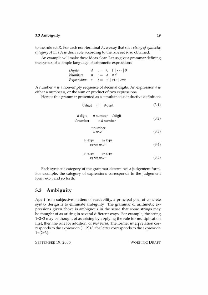
An example will make these ideas clear. Let us give a grammar definingthe syntax of a simple language of arithmetic expressions.
Digits d : : = 0 | 1 | · · · | 9Numbers n : : = d | n dExpressions e : : = n | e+e | e*e
A number n is a non-empty sequence of decimal digits. An expression e iseither a number n, or the sum or product of two expressions.
Here is this grammar presented as a simultaneous inductive definition:
0 digit · · · 9 digit (3.1)
d digit
d number
n number d digit
n d number(3.2)
n numbern expr (3.3)
e1 expr e2 expre1+e2 expr (3.4)
e1 expr e2 expre1*e2 expr (3.5)
Each syntactic category of the grammar determines a judgement form.For example, the category of expressions corresponds to the judgementform expr, and so forth.
3.3 Ambiguity
Apart from subjective matters of readability, a principal goal of concretesyntax design is to eliminate ambiguity. The grammar of arithmetic ex-pressions given above is ambiguous in the sense that some strings maybe thought of as arising in several different ways. For example, the string1+2*3 may be thought of as arising by applying the rule for multiplicationfirst, then the rule for addition, or vice versa. The former interpretation cor-responds to the expression (1+2)*3; the latter corresponds to the expression1+(2*3).
SEPTEMBER 19, 2005 WORKING DRAFT
20 3.3 Ambiguity
The trouble is that we cannot simply tell from the generated stringwhich reading is intended. This causes numerous problems. For exam-ple, suppose that we wish to define a function eval that assigns to eacharithmetic expression e its value n ∈ N. A natural approach is to use ruleinduction on the rules determined by the grammar of expressions.
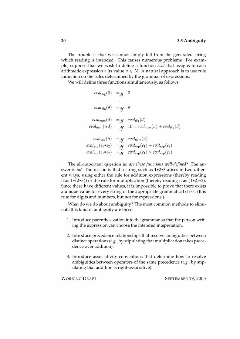
We will define three functions simultaneously, as follows:
evaldig(0) =df 0...
evaldig(9) =df 9
evalnum(d) =df evaldig(d)evalnum(n d) =df 10× evalnum(n) + evaldig(d)
evalexp(n) =df evalnum(n)evalexp(e1+e2) =df evalexp(e1) + evalexp(e2)evalexp(e1*e2) =df evalexp(e1)× evalexp(e2)
The all-important question is: are these functions well-defined? The an-swer is no! The reason is that a string such as 1+2*3 arises in two differ-ent ways, using either the rule for addition expressions (thereby readingit as 1+(2*3)) or the rule for multiplication (thereby reading it as (1+2)*3).Since these have different values, it is impossible to prove that there existsa unique value for every string of the appropriate grammatical class. (It istrue for digits and numbers, but not for expressions.)
What do we do about ambiguity? The most common methods to elimi-nate this kind of ambiguity are these:
1. Introduce parenthesization into the grammar so that the person writ-ing the expression can choose the intended intepretation.
2. Introduce precedence relationships that resolve ambiguities betweendistinct operations (e.g., by stipulating that multiplication takes prece-dence over addition).
3. Introduce associativity conventions that determine how to resolveambiguities between operators of the same precedence (e.g., by stip-ulating that addition is right-associative).
WORKING DRAFT SEPTEMBER 19, 2005

3.3 Ambiguity 21
Using these techniques, we arrive at the following revised grammar forarithmetic expressions.
Digits d : : = 0 | 1 | · · · | 9Numbers n : : = d | n dExpressions e : : = t | t+eTerms t : : = f | f*tFactors f : : = n | (e)
We have made two significant changes. The grammar has been “layered”to express the precedence of multiplication over addition and to expressright-associativity of each, and an additional form of expression, parenthe-sization, has been introduced.
It is a straightforward exercise to translate this grammar into an induc-tive definition. Having done so, it is also straightforward to revise the def-inition of the evaluation functions so that are well-defined. The reviseddefinitions are given by rule induction; they require additional clauses forthe new syntactic categories.
evaldig(0) =df 0...
evaldig(9) =df 9
evalnum(d) =df evaldig(d)evalnum(n d) =df 10× evalnum(n) + evaldig(d)
evalexp(t) =df evaltrm(t)evalexp(t+e) =df evaltrm(t) + evalexp(e)
evaltrm( f ) =df evalfct( f )evaltrm( f*t) =df evalfct( f )× evaltrm(t)
evalfct(n) =df evalnum(n)evalfct((e)) =df evalexp(e)
A straightforward proof by rule induction shows that these functions arewell-defined.
SEPTEMBER 19, 2005 WORKING DRAFT
22 3.4 Exercises
3.4 Exercises
WORKING DRAFT SEPTEMBER 19, 2005
Chapter 4
Abstract Syntax Trees
The concrete syntax of a language is an inductively-defined set of stringsover a given alphabet. Its abstract syntax is an inductively-defined set ofabstract syntax trees, or ast’s, over a set of operators. Abstract syntax avoidsthe ambiguities of concrete syntax by employing operators that determinethe outermost form of any given expression, rather than relying on parsingconventions to disambiguate strings.
4.1 Abstract Syntax Trees
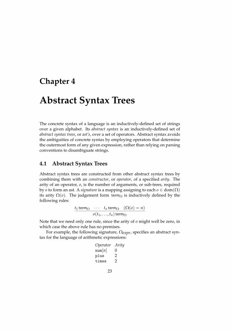
Abstract syntax trees are constructed from other abstract syntax trees bycombining them with an constructor, or operator, of a specified arity. Thearity of an operator, o, is the number of arguments, or sub-trees, requiredby o to form an ast. A signature is a mapping assigning to each o ∈ dom(Ω)its arity Ω(o). The judgement form termΩ is inductively defined by thefollowing rules:
t1 termΩ · · · tn termΩ (Ω(o) = n)o(t1, . . . , tn) termΩ
Note that we need only one rule, since the arity of o might well be zero, inwhich case the above rule has no premises.
For example, the following signature, Ωexpr, specifies an abstract syn-tax for the language of arithmetic expressions:
Operator Aritynum[n] 0plus 2times 2
23
24 4.2 Structural Induction
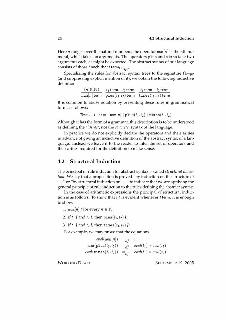
Here n ranges over the natural numbers; the operator num[n] is the nth nu-meral, which takes no arguments. The operators plus and times take twoarguments each, as might be expected. The abstract syntax of our languageconsists of those t such that t termΩexpr .
Specializing the rules for abstract syntax trees to the signature Ωexpr(and suppressing explicit mention of it), we obtain the following inductivedefinition:
(n ∈N)num[n] term
t1 term t2 term
plus(t1, t2) term
t1 term t2 term
times(t1, t2) term
It is common to abuse notation by presenting these rules in grammaticalform, as follows:
Terms t : : = num[n] | plus(t1, t2) | times(t1, t2)
Although it has the form of a grammar, this description is to be understoodas defining the abstract, not the concrete, syntax of the language.
In practice we do not explicitly declare the operators and their aritiesin advance of giving an inductive definition of the abstract syntax of a lan-guage. Instead we leave it to the reader to infer the set of operators andtheir arities required for the definition to make sense.
4.2 Structural Induction
The principal of rule induction for abstract syntax is called structural induc-tion. We say that a proposition is proved “by induction on the structure of. . . ” or “by structural induction on . . . ” to indicate that we are applying thegeneral principle of rule induction to the rules defining the abstract syntax.
In the case of arithmetic expressions the principal of structural induc-tion is as follows. To show that t J is evident whenever t term, it is enoughto show:
1. num[n] J for every n ∈N;
2. if t1 J and t2 J, then plus(t1, t2) J;
3. if t1 J and t2 J, then times(t1, t2) J;
For example, we may prove that the equations
eval(num[n]) =df neval(plus(t1, t2)) =df eval(t1) + eval(t2)
eval(times(t1, t2)) =df eval(t1)× eval(t2)
WORKING DRAFT SEPTEMBER 19, 2005
4.3 Parsing 25
determine a function eval from the abstract syntax of expressions to num-bers. That is, we may show by induction on the structure of e that there isa unique n such that eval(t) = n.
4.3 Parsing
The process of translation from concrete to abstract syntax is called pars-ing. Typically the concrete syntax is specified by an inductive definitiondefining the grammatical strings of the language, and the abstract syntax isgiven by an inductive definition of the abstract syntax trees that constitutethe language. In this case it is natural to formulate parsing as an inductivelydefined function mapping concrete the abstract syntax. Since parsing is tobe a function, there is exactly one abstract syntax tree corresponding to awell-formed (grammatical) piece of concrete syntax. Strings that are notderivable according to the rules of the concrete syntax are not grammatical,and can be rejected as ill-formed.
For example, consider the language of arithmetic expressions discussedin Chapter 3. Since we wish to define a function on the concrete syntax, itshould be clear from the discussion in Section 3.3 that we should workwith the disambiguated grammar that makes explicit the precedence andassociativity of addition and multiplication. With the rules of this grammarin mind, we may define simultaneously a family of parsing functions for
SEPTEMBER 19, 2005 WORKING DRAFT
26 4.3 Parsing
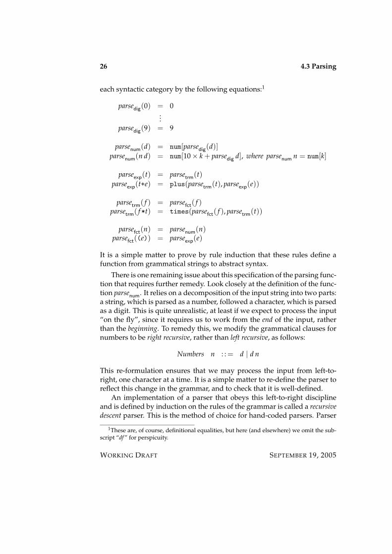
each syntactic category by the following equations:1
parsedig(0) = 0...
parsedig(9) = 9
parsenum(d) = num[parsedig(d)]parsenum(n d) = num[10× k + parsedig d], where parsenum n = num[k]
parseexp(t) = parsetrm(t)parseexp(t+e) = plus(parsetrm(t), parseexp(e))
parsetrm( f ) = parsefct( f )parsetrm( f*t) = times(parsefct( f ), parsetrm(t))
parsefct(n) = parsenum(n)parsefct((e)) = parseexp(e)
It is a simple matter to prove by rule induction that these rules define afunction from grammatical strings to abstract syntax.
There is one remaining issue about this specification of the parsing func-tion that requires further remedy. Look closely at the definition of the func-tion parsenum. It relies on a decomposition of the input string into two parts:a string, which is parsed as a number, followed a character, which is parsedas a digit. This is quite unrealistic, at least if we expect to process the input“on the fly”, since it requires us to work from the end of the input, ratherthan the beginning. To remedy this, we modify the grammatical clauses fornumbers to be right recursive, rather than left recursive, as follows:
Numbers n : : = d | d n
This re-formulation ensures that we may process the input from left-to-right, one character at a time. It is a simple matter to re-define the parser toreflect this change in the grammar, and to check that it is well-defined.
An implementation of a parser that obeys this left-to-right disciplineand is defined by induction on the rules of the grammar is called a recursivedescent parser. This is the method of choice for hand-coded parsers. Parser
1These are, of course, definitional equalities, but here (and elsewhere) we omit the sub-script “df ” for perspicuity.
WORKING DRAFT SEPTEMBER 19, 2005
4.4 Exercises 27
generators, which automatically create parsers from grammars, make useof a different technique that is more efficient, but much harder to imple-ment by hand.
4.4 Exercises
1. Give a concrete and (first-order) abstract syntax for a language.
2. Write a parser for that language.
SEPTEMBER 19, 2005 WORKING DRAFT

28 4.4 Exercises
WORKING DRAFT SEPTEMBER 19, 2005
Chapter 5
Abstract Binding Trees
Abstract syntax trees make explicit the hierarchical relationships among thecomponents of a phrase by abstracting out from irrelevant surface detailssuch as parenthesization. Abstract binding trees, or abt’s, go one step furtherand make explicit the binding and scope of identifiers in a phrase, abstract-ing from the “spelling” of bound names so as to focus attention on theirfundamental role as designators.
5.1 Names
Names are widely used in programming languages: names of variables,names of fields in structures, names of types, names of communicationchannels, names of locations in the heap, and so forth. Names have nostructure beyond their identity. In particular, the “spelling” of a name isof no intrinsic significance, but serves only to distinguish one name fromanother. Consequently, we shall treat names as atoms, and abstract awaytheir internal structure.
We assume given a judgement form name such that x name for infinitelymany x. We will often make use of n-tuples of names ~x = x1, . . . , xn, wheren ≥ 0. The constituent names of ~x are written xi, where 1 ≤ i ≤ n, andwe tacitly assume that if i 6= j, then xi and xj are distinct names. In anysuch tuple the names xi are tacitly assumed to be pairwise distinct. If ~x isan n-tuple of names, we define its length, |~x|, to be n.
29

30 5.2 Abstract Syntax With Names
5.2 Abstract Syntax With Names
Suppose that we enrich the language of arithmetic expressions given inChapter 4 with a means of binding the value of an arithmetic expression toan identifier for use within another arithmetic expression. To support thiswe extend the abstract syntax with two additional constructs:1
x nameid(x) termΩ
x name t1 termΩ t2 termΩ
let(x, t1, t2) termΩ
The ast id(x) represents a use of a name, x, as a variable, and the astlet(x, t1, t2) introduces a name, x, that is to be bound to (the value of) t1for use within t2.
The difficulty with abstract syntax trees is that they make no provisionfor specifying the binding and scope of names. For example, in the astlet(x, t1, t2), the name x is available for use within t2, but not within t1.That is, the name x is bound by the let construct for use within its scope,the sub-tree t2. But there is nothing intrinsic to the ast that makes this clear.Rather, it is a condition imposed on the ast “from the outside”, rather thanan intrinsic property of the abstract syntax. Worse, the informal specifica-tion is vague in certain respects. For example, what does it mean if we nestbindings for the same identifier, as in the following example?
let(x, t1, let(x, id(x), id(x)))
Which occurrences of x refer to which bindings, and why?
5.3 Abstract Binding Trees
Abstract binding trees are a generalization of abstract syntax trees that pro-vide intrinsic support for binding and scope of names. Abt’s are formedfrom names and abstractors by operators. Operators are assigned (general-ized) arities, which are finite sequences of valences, which are natural num-bers. Thus an arity has the form (m1, . . . , mk), specifying an operator with karguments, each of which is an abstractor of the specified valence. Abstrac-tors are formed by associating zero or more names with an abt; the valenceis the number of names attached to the abstractor. The present notion ofarity generalizes that given in Chapter 4 by observing that the arity n fromChapter 4 becomes the arity (0, . . . , 0), with n copies of 0.
1One may also devise a concrete syntax, for example writing let x be e1 in e2 for thebinding construct, and a parser to translate from the concrete to the abstract syntax.
WORKING DRAFT SEPTEMBER 19, 2005

5.4 Renaming 31
This informal description can be made precise by a simultaneous induc-tive definition of two judgement forms, abtΩ and absΩ, which are param-eterized by a signature assigning a (generalized) arity to each of a finite setof operators. The judgement t abtΩ asserts that t is an abt over signature Ω,and the judgement ~x.t absn
Ω states that ~x.t is an abstractor of valence n.
x namex abtΩ
β1 absm1Ω · · · βk absmk
Ω
o(β1, . . . , βk) abtΩ(Ω(o) = (m1, . . . , mk))
t abtΩ
t abs0Ω
x name β absnΩ
x.β absn+1Ω
An abstractor of valence n has the form x1.x2.. . . xn.t, which is sometimesabbreviated ~x.t, where ~x = x1, . . . , xn. We tacitly assume that no nameis repeated in such a sequence, since doing so serves no useful purpose.Finally, we make no distinction between an abstractor of valence zero andan abt.
The language of arithmetic expressions may be represented as abstractbinding trees built from the following signature.
Operator Aritynum[n] ()plus (0, 0)times (0, 0)let (0, 1)
The arity of the “let” operator makes clear that no name is bound in thefirst position, but that one name is bound in the second.
5.4 Renaming
The free names, FN(t), of an abt, t, is inductively defined by the followingrecursion equations:
FN(x) =df x FN(o(β1, . . . , βk)) =df FN(β1) ∪ · · · ∪ FN(βk)
FN(~x.t) =df FN(t) \~x
Thus, the set of free names in t are those names occurring in t that do not liewithin the scope of an abstractor.
SEPTEMBER 19, 2005 WORKING DRAFT
32 5.4 Renaming
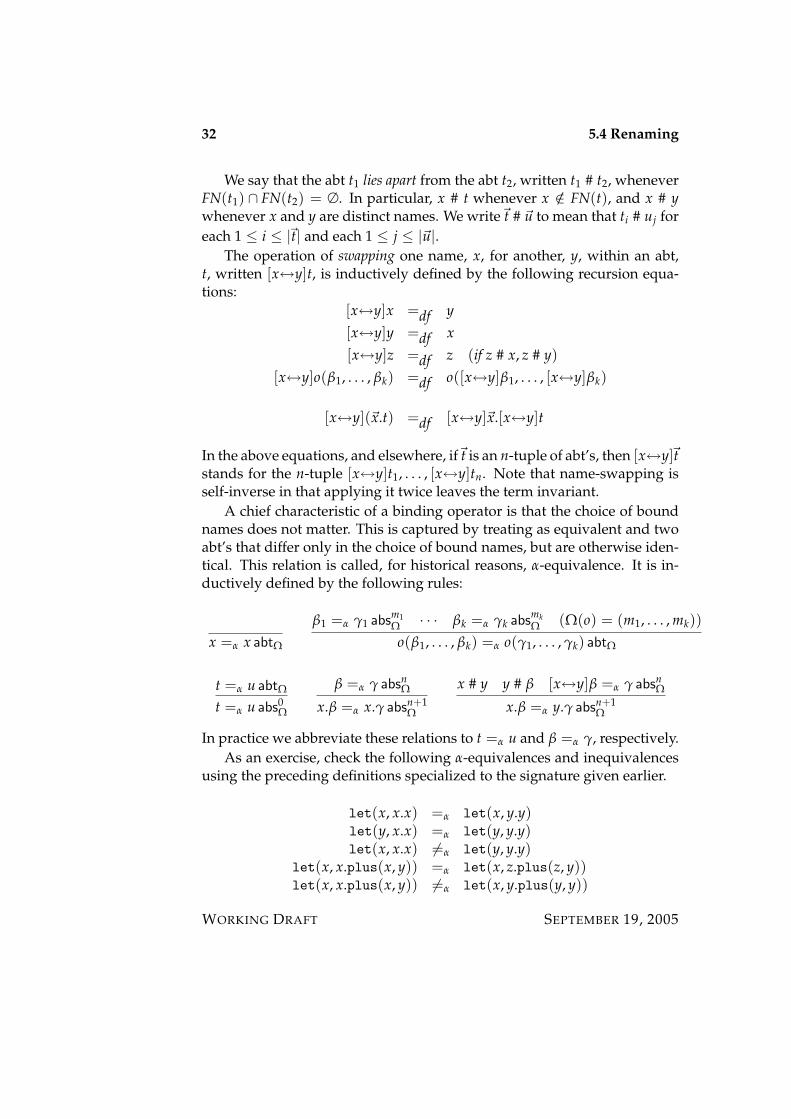
We say that the abt t1 lies apart from the abt t2, written t1 # t2, wheneverFN(t1) ∩ FN(t2) = ∅. In particular, x # t whenever x /∈ FN(t), and x # ywhenever x and y are distinct names. We write~t # ~u to mean that ti # uj foreach 1 ≤ i ≤ |~t| and each 1 ≤ j ≤ |~u|.
The operation of swapping one name, x, for another, y, within an abt,t, written [x↔y]t, is inductively defined by the following recursion equa-tions:
[x↔y]x =df y[x↔y]y =df x[x↔y]z =df z (if z # x, z # y)
[x↔y]o(β1, . . . , βk) =df o([x↔y]β1, . . . , [x↔y]βk)
[x↔y](~x.t) =df [x↔y]~x.[x↔y]t
In the above equations, and elsewhere, if~t is an n-tuple of abt’s, then [x↔y]~tstands for the n-tuple [x↔y]t1, . . . , [x↔y]tn. Note that name-swapping isself-inverse in that applying it twice leaves the term invariant.
A chief characteristic of a binding operator is that the choice of boundnames does not matter. This is captured by treating as equivalent and twoabt’s that differ only in the choice of bound names, but are otherwise iden-tical. This relation is called, for historical reasons, α-equivalence. It is in-ductively defined by the following rules:
x =α x abtΩ
β1 =α γ1 absm1Ω · · · βk =α γk absmk
Ω (Ω(o) = (m1, . . . , mk))o(β1, . . . , βk) =α o(γ1, . . . , γk) abtΩ
t =α u abtΩ
t =α u abs0Ω
β =α γ absnΩ
x.β =α x.γ absn+1Ω
x # y y # β [x↔y]β =α γ absnΩ
x.β =α y.γ absn+1Ω
In practice we abbreviate these relations to t =α u and β =α γ, respectively.As an exercise, check the following α-equivalences and inequivalences
using the preceding definitions specialized to the signature given earlier.
let(x, x.x) =α let(x, y.y)let(y, x.x) =α let(y, y.y)let(x, x.x) 6=α let(y, y.y)
let(x, x.plus(x, y)) =α let(x, z.plus(z, y))let(x, x.plus(x, y)) 6=α let(x, y.plus(y, y))
WORKING DRAFT SEPTEMBER 19, 2005

5.4 Renaming 33
The following axiom of α-equivalence is derivable:
x # y y # β
x.β =α y.[x↔y]β absn+1Ω
This is often stated as the fundamental axiom of α-equivalence. Finally, ob-serve that if t =α u abtΩ, then FN(t) = FN(u), and similarly if β =α γ absn
Ω,then FN(β) = FN(γ). In particular, if t =α u abtΩ and x # u, then x # t.
It may be shown by rule induction that α-equivalence is, in fact, anequivalence relation (i.e., it is reflexive, symmetric, and transitive). Forsymmetry we that the free name set is invariant under α-equivalence, andthat name-swapping is self-inverse. For transitivity we must show simul-taneously that (i) t =α u and u =α v imply t =α v, and (ii) β =α γ andγ =α δ imply β =α δ. Let us consider the case that β = x.β′, γ = y.γ′, andδ = z.δ′. Suppose that β =α γ and γ =α δ. We are to show that β =α δ, forwhich it suffices to show either
1. x = z and β′ =α δ′, or
2. x # z and z # β′ and [x↔z]β′ =α δ′.
There are four cases to consider, depending on the derivation of β =α γand γ =α δ. Consider the case in which x # y, y # β′, and [x↔y]β′ =α γ′
from the first assumption, and y # z, z # γ′, and [y↔z]γ′ =α δ′ from thesecond. We proceed by cases on whether x = z or x # z.
1. Suppose that x = z. Since [x↔y]β′ =α γ′ and [y↔z]γ′ =α δ′, it fol-lows that [y↔z][x↔y]β′ =α δ′. But since x = z, we have [y↔z][x↔y]β′ =[y↔x][x↔y]β′ = β′, so we have β′ =α δ′, as desired.
2. Suppose that x # z. Note that z # γ′, so z # [x↔y]β′, and hence z # β′
since x # z and y # z. Finally, [x↔y]β′ =α γ′, so [y↔z][x↔y]β′ =α δ′,and hence [x↔z]β′ =α δ′, as required.
This completes the proof of this case; the other cases are handled similarly.From this point onwards we identify any two abt’s t and u such that
t =α u. This means that an abt implicitly stands for its α-equivalence class,and that we tacitly assert that all operations and relations on abt’s respectsα-equivalence. Put the other way around, any operation or relation on abt’sthat fails to respect α-equivalence is illegitimate, and therefore ruled out ofconsideration. In this way we ensure that the choice of bound names doesnot matter.
SEPTEMBER 19, 2005 WORKING DRAFT
34 5.5 Structural Induction
One consequence of this policy on abt’s is that whenever we encounteran abstract x.β, we may assume that x is fresh in the sense that it may beimplicitly chosen to not occur in any specified finite set of names. For if Xis such a finite set and x ∈ X, then we may choose another representativeof the α-equivalence class of x.β, say x′.β′, such that x′ /∈ X, meeting theimplicit assumption of freshness.
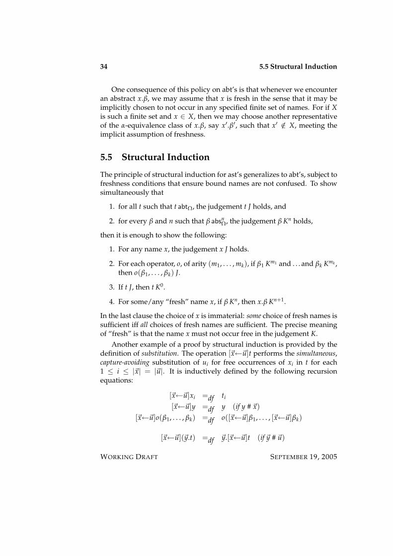
5.5 Structural Induction
The principle of structural induction for ast’s generalizes to abt’s, subject tofreshness conditions that ensure bound names are not confused. To showsimultaneously that
1. for all t such that t abtΩ, the judgement t J holds, and
2. for every β and n such that β absnΩ, the judgement β Kn holds,
then it is enough to show the following:
1. For any name x, the judgement x J holds.
2. For each operator, o, of arity (m1, . . . , mk), if β1 Km1 and . . . and βk Kmk ,then o(β1, . . . , βk) J.
3. If t J, then t K0.
4. For some/any “fresh” name x, if β Kn, then x.β Kn+1.
In the last clause the choice of x is immaterial: some choice of fresh names issufficient iff all choices of fresh names are sufficient. The precise meaningof “fresh” is that the name x must not occur free in the judgement K.
Another example of a proof by structural induction is provided by thedefinition of substitution. The operation [~x←~u]t performs the simultaneous,capture-avoiding substitution of ui for free occurrences of xi in t for each1 ≤ i ≤ |~x| = |~u|. It is inductively defined by the following recursionequations:
[~x←~u]xi =df ti
[~x←~u]y =df y (if y # ~x)[~x←~u]o(β1, . . . , βk) =df o([~x←~u]β1, . . . , [~x←~u]βk)
[~x←~u](~y.t) =df ~y.[~x←~u]t (if ~y # ~u)
WORKING DRAFT SEPTEMBER 19, 2005
5.5 Structural Induction 35
The condition on the last clause can always be met, by the freshness as-sumption. More precisely, we may prove by structural induction that sub-stitution is total in the sense that for any ~u, ~x, and t, there exists a unique t′
such that [~x←~u]t = t′. The crucial point is that the principal of structuralinduction for abstract binding trees permits us to choose bound names tolie apart from ~x when applying the inductive hypothesis.
SEPTEMBER 19, 2005 WORKING DRAFT

36 5.5 Structural Induction
WORKING DRAFT SEPTEMBER 19, 2005

Chapter 6
Static Semantics
The static semantics of a language determines which pieces of abstract syn-tax (represented as ast’s or abt’s) are well-formed according to some context-sensitive criteria. A typical example of a well-formedness constraint is scoperesolution, the requirement that every name be declared before it is used.
6.1 Static Semantics of Arithmetic Expressions
We will give an inductive definition of a static semantics for the languageof arithmetic expressions that performs scope resolution. A well-formednessjudgement has the form Γ ` e ok, where Γ is a finite set of variables and eis the abt representation of an arithmetic expression. The meaning of thisjudgement is that e is an arithmetic expression all of whose free variablesare in the set Γ. Thus, if ∅ ` e ok, then e has no unbound variables, and istherefore suitable for evaluation.
(x ∈ Γ)Γ ` x ok
(n ≥ 0)Γ ` num[n] ok
Γ ` e1 ok Γ ` e2 ok
Γ ` plus(e1, e2) ok
Γ ` e1 ok Γ ` e2 ok
Γ ` times(e1, e2) ok
Γ ` e1 ok Γ ∪ x ` e2 ok (x /∈ Γ)Γ ` let(e1, x.e2) ok
There are a few things to notice about these rules. First, a variable is well-formed iff it is in Γ. This is consistent with the informal reading of thejudgement. Second, a let expression adds a new variable to Γ for use within
37
38 6.2 Exercises
e2. The “newness” of the variable is captured by the requirement that x /∈ Γ.Since we identify abt’s up to choice of bound names, this requirement canalways be met by a suitable renaming prior to application of the rule. Third,the rules are syntax-directed in the sense that there is one rule for each formof expression; as we will see later, this is not always the case for a staticsemantics.
6.2 Exercises
1. Show that Γ ` e ok iff FN(e) ⊆ Γ. From left to right, proceed by ruleinduction. From right to left, proceed by induction on the structureof e.
WORKING DRAFT SEPTEMBER 19, 2005
Chapter 7
Dynamic Semantics
The dynamic semantics of a language specifies how programs are to be ex-ecuted. There are two popular methods for specifying dynamic seman-tics. One method, called structured operational semantics (SOS), or transi-tion semantics, presents the dynamic semantics of a language as a transitionsystem specifying the step-by-step execution of programs. Another, calledevaluation semantics, or ES, presents the dynamic semantics as a binary re-lation specifying the result of a complete execution of a program.
7.1 Structured Operational Semantics
A structured operational semantics for a language consists of a transitionsystem whose states are programs and whose transition relation is definedby induction over the structure of programs. We will illustrate SOS forthe simple language of arithmetic expressions (including let expressions)discussed in Chapter 5.
The set of states is the set of well-formed arithmetic expressions:
S = e | ∃Γ Γ ` e ok .
The set of initial states, I ⊆ S, is the set of closed expressions:
I = e | ∅ ` e ok .
The set of final states, F ⊆ S, is just the set of numerals for natural numbers:
F = num[n] | n ≥ 0 .
39
40 7.1 Structured Operational Semantics
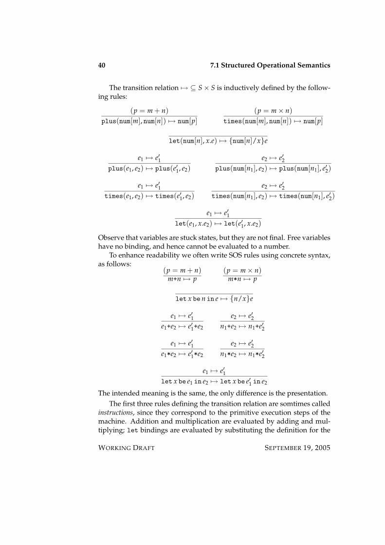
The transition relation 7→ ⊆ S× S is inductively defined by the follow-ing rules:
(p = m + n)plus(num[m], num[n]) 7→ num[p]
(p = m× n)times(num[m], num[n]) 7→ num[p]
let(num[n], x.e) 7→ num[n]/xe
e1 7→ e′1plus(e1, e2) 7→ plus(e′1, e2)
e2 7→ e′2plus(num[n1], e2) 7→ plus(num[n1], e′2)
e1 7→ e′1times(e1, e2) 7→ times(e′1, e2)
e2 7→ e′2times(num[n1], e2) 7→ times(num[n1], e′2)
e1 7→ e′1let(e1, x.e2) 7→ let(e′1, x.e2)
Observe that variables are stuck states, but they are not final. Free variableshave no binding, and hence cannot be evaluated to a number.
To enhance readability we often write SOS rules using concrete syntax,as follows:
(p = m + n)m+n 7→ p
(p = m× n)m*n 7→ p
let x be n in e 7→ n/xe
e1 7→ e′1e1+e2 7→ e′1+e2
e2 7→ e′2n1+e2 7→ n1+e′2
e1 7→ e′1e1*e2 7→ e′1*e2
e2 7→ e′2n1*e2 7→ n1*e′2
e1 7→ e′1let x be e1 in e2 7→ let x be e′1 in e2
The intended meaning is the same, the only difference is the presentation.The first three rules defining the transition relation are somtimes called
instructions, since they correspond to the primitive execution steps of themachine. Addition and multiplication are evaluated by adding and mul-tiplying; let bindings are evaluated by substituting the definition for the
WORKING DRAFT SEPTEMBER 19, 2005

7.1 Structured Operational Semantics 41
variable in the body. In all three cases the principal arguments of the con-structor are required to be numbers. Both arguments of an addition ormultiplication are principal, but only the binding of the variable in a letexpression is principal. We say that these primitives are evaluated by value,because the instructions apply only when the principal arguments havebeen fully evaluated.
What if the principal arguments have not (yet) been fully evaluated?Then we must evaluate them! In the case of arithmetic expressions we ar-bitrarily choose a left-to-right evaluation order. First we evaluate the firstargument, then the second. Once both have been evaluated, the instructionrule applies. In the case of let expressions we first evaluate the binding,after which the instruction step applies. Note that evaluation of an argu-ment can take multiple steps. The transition relation is defined so that onestep of evaluation is made at a time, reconstructing the entire expression asnecessary.
For example, consider the following evaluation sequence:
let x be 1+2 in (x+3)*4 7→ let x be 3 in (x+3)*47→ (3+3)*47→ 6*47→ 24
Each step is justified by a rule defining the transition relation. Instructionrules are axioms, and hence have no premises, but all other rules are justi-fied by a subsidiary deduction of another transition. For example, the firsttransition is justified by a subsidiary deduction of 1+2 7→ 3, which is justi-fied by the first instruction rule definining the transition relation. Each ofthe subsequent steps is justified similarly.
Since the transition relation in SOS is inductively defined, we may rea-son about it using rule induction. Specifically, to show that P(e, e′) holdswhenever e 7→ e′, it is sufficient to show that P is closed under the rulesdefining the transition relation. For example, it is a simple matter to showby rule induction that the transition relation for evaluation of arithmetic ex-pressions is deterministic: if e 7→ e′ and e 7→ e′′, then e′ = e′′. This may beproved by simultaneous rule induction over the definition of the transitionrelation.
SEPTEMBER 19, 2005 WORKING DRAFT
42 7.2 Evaluation Semantics
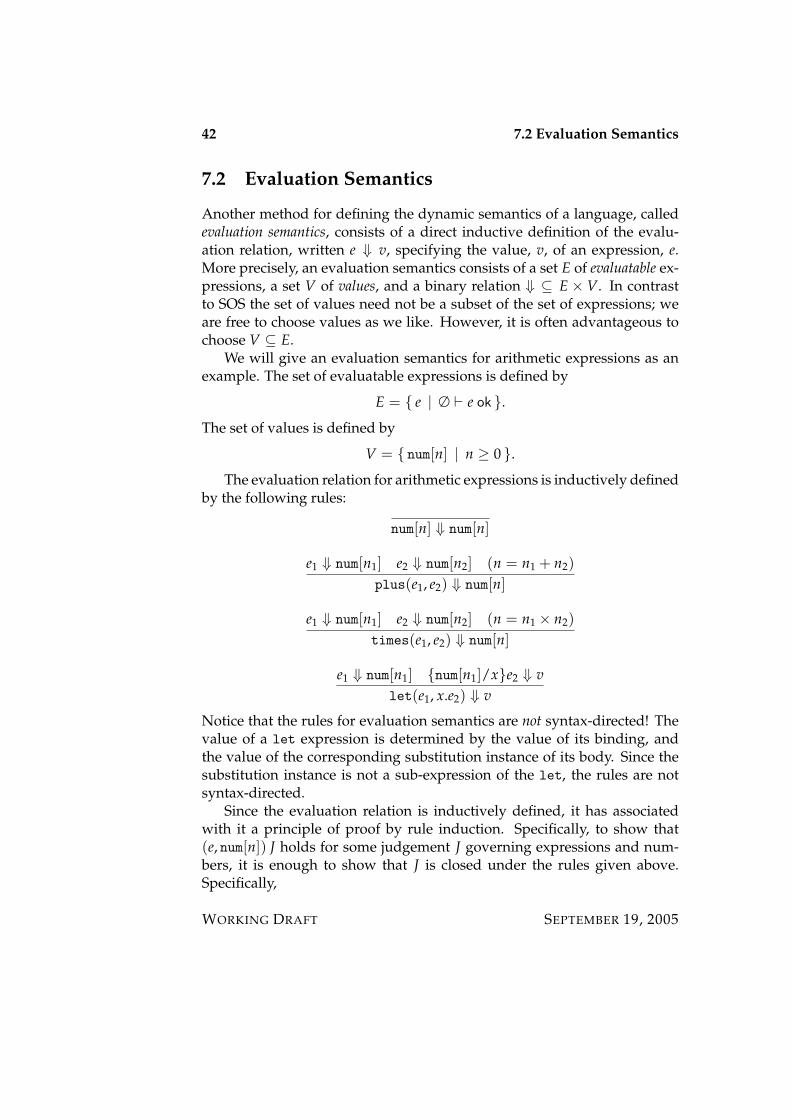
7.2 Evaluation Semantics
Another method for defining the dynamic semantics of a language, calledevaluation semantics, consists of a direct inductive definition of the evalu-ation relation, written e ⇓ v, specifying the value, v, of an expression, e.More precisely, an evaluation semantics consists of a set E of evaluatable ex-pressions, a set V of values, and a binary relation ⇓ ⊆ E × V. In contrastto SOS the set of values need not be a subset of the set of expressions; weare free to choose values as we like. However, it is often advantageous tochoose V ⊆ E.
We will give an evaluation semantics for arithmetic expressions as anexample. The set of evaluatable expressions is defined by
E = e | ∅ ` e ok .
The set of values is defined by
V = num[n] | n ≥ 0 .
The evaluation relation for arithmetic expressions is inductively definedby the following rules:
num[n] ⇓ num[n]
e1 ⇓ num[n1] e2 ⇓ num[n2] (n = n1 + n2)plus(e1, e2) ⇓ num[n]
e1 ⇓ num[n1] e2 ⇓ num[n2] (n = n1 × n2)times(e1, e2) ⇓ num[n]
e1 ⇓ num[n1] num[n1]/xe2 ⇓ vlet(e1, x.e2) ⇓ v
Notice that the rules for evaluation semantics are not syntax-directed! Thevalue of a let expression is determined by the value of its binding, andthe value of the corresponding substitution instance of its body. Since thesubstitution instance is not a sub-expression of the let, the rules are notsyntax-directed.
Since the evaluation relation is inductively defined, it has associatedwith it a principle of proof by rule induction. Specifically, to show that(e, num[n]) J holds for some judgement J governing expressions and num-bers, it is enough to show that J is closed under the rules given above.Specifically,
WORKING DRAFT SEPTEMBER 19, 2005

7.3 Relating Transition and Evaluation Semantics 43
1. Show that (num[n], num[n]) J.
2. Assume that (e1, num[n1]) J and (e2, num[n2]) J. Show that (plus(e1, e2), num[n1 + n2]) Jand that (times(e1, e2), num[n1 × n2]) J.
3. Assume that (e1, num[n1]) J and (num[n1]/xe2, num[n2]) J. Show that(let(e1, x.e2), num[n2]) J.
7.3 Relating Transition and Evaluation Semantics
We have given two different forms of dynamic semantics for the same lan-guage. It is natural to ask whether they are equivalent, but to do so first re-quires that we consider carefully what we mean by equivalence. The tran-sition semantics describes a step-by-step process of execution, whereas theevaluation semantics suppresses the intermediate states, focussing atten-tion on the initial and final states alone. This suggests that the appropriatecorrespondence is between complete execution sequences in the transitionsemantics and the evaluation relation in the evaluation semantics.
Theorem 7.1For all well-formed, closed arithmetic expressions e and all natural num-
bers n, e !7→ num[n] iff e ⇓ num[n].
How might we prove such a theorem? We will consider each directionseparately. We consider the easier case first.
Lemma 7.2If e ⇓ num[n], then e !7→ num[n].
Proof: By induction on the definition of the evaluation relation. For exam-ple, suppose that plus(e1, e2) ⇓ num[n] by the rule for evaluating additions.
By induction we know that e1!7→ num[n1] and e2
!7→ num[n2]. We reason asfollows:
plus(e1, e2)∗7→ plus(num[n1], e2)∗7→ plus(num[n1], num[n2])7→ num[n1 + n2]
Therefore plus(e1, e2)!7→ num[n1 + n2], as required. The other cases are han-
dled similarly.
SEPTEMBER 19, 2005 WORKING DRAFT
44 7.4 Exercises
What about the converse? Recall from Chapter 2 that the complete eval-
uation relation, !7→, is the restriction of the multi-step evaluation relation,∗7→, to initial and final states (here closed expressions and numerals). Recall
also that multi-step evaluation is inductively defined by two rules, reflex-ivity and closure under head expansion. By definition num[n] ⇓ num[n], soit suffices to show closure under head expansion.
Lemma 7.3If e 7→ e′ and e′ ⇓ num[n], then e ⇓ num[n].
Proof: By induction on the definition of the transition relation. For ex-ample, suppose that plus(e1, e2) 7→ plus(e′1, e2), where e1 7→ e′1. Supposefurther that plus(e′1, e2) ⇓ num[n], so that e′1 ⇓ num[n1], and e2 ⇓ num[n2]and n = n1 + n2. By induction e1 ⇓ num[n1], and hence plus(e1, e2) ⇓ n, asrequired.
7.4 Exercises
1. Prove that if e 7→ e1 and e 7→ e2, then e1 ≡ e2.
2. Prove that if e ∈ I and e 7→ e′, then e′ ∈ I. Proceed by induction onthe definition of the transition relation.
3. Prove that if e ∈ I \ F, then there exists e′ such that e 7→ e′. Proceed byinduction on the rules defining well-formedness given in Chapter 6.
4. Prove that if e ⇓ v1 and e ⇓ v2, then v1 ≡ v2.
5. Complete the proof of equivalence of evaluation and transition se-mantics.
WORKING DRAFT SEPTEMBER 19, 2005
Chapter 8
Relating Static and DynamicSemantics
The static and dynamic semantics of a language cohere if the strictures ofthe static semantics ensure the well-behavior of the dynamic semantics. Inthe case of arithmetic expressions, this amounts to showing two properties:
1. Preservation: If ∅ ` e ok and e 7→ e′, then ∅ ` e′ ok.
2. Progress: If ∅ ` e ok, then either e = num[n] for some n, or there existse′ such that e 7→ e′.
The first says that the steps of evaluation preserve well-formedness, thesecond says that well-formedness ensures that either we are done or wecan make progress towards completion.
8.1 Preservation for Arithmetic Expressions
The preservation theorem is proved by induction on the rules defining thetransition system for step-by-step evaluation of arithmetic expressions. Wewill write e ok for ∅ ` e ok to enhance readability. Consider the rule
e1 7→ e′1plus(e1, e2) 7→ plus(e′1, e2).
By induction we may assume that if e1 ok, then e′1 ok. Assume that plus(e1, e2) ok.From the definition of the static semantics we have that e1 ok and e2 ok. Byinduction e′1 ok, so by the static semantics plus(e′1, e2) ok. The other casesare quite similar.
45
46 8.2 Progress for Arithmetic Expressions
8.2 Progress for Arithmetic Expressions
A moment’s thought reveals that if e 6 7→, then e must be a name, for other-wise e is either a number or some transition applies. Thus the content of theprogress theorem for the language of arithmetic expressions is that evalua-tion of a well-formed expression cannot encounter an unbound variable.
The proof of progress proceeds by induction on the rules of the staticsemantics. The rule for variables cannot occur, because we are assumingthat the context, Γ, is empty. To take a representative case, consider the rule
Γ ` e1 ok Γ ` e2 ok
Γ ` plus(e1, e2) ok
where Γ = ∅. Let e = plus(e1, e2), and assume e ok. Since e is not anumber, we must show that there exists e′ such that e 7→ e′. By induc-tion we have that either e1 is a number, num[n1], or there exists e′1 suchthat e1 7→ e′1. In the latter case it follows that plus(e1, e2) 7→ plus(e′1, e2),as required. In the former we also have by induction that either e2 is anumber, num[n2], or there exists e′2 such that e1 7→ e′1. In the latter casewe have plus(num[n1], e2) 7→ plus(num[n2], e′2). In the former we haveplus(num[n1], num[n2]) 7→ num[n1 + n2]. The other cases are handled sim-ilarly.
8.3 Exercises
WORKING DRAFT SEPTEMBER 19, 2005
Part III
A Functional Language
47

Chapter 9
A Minimal FunctionalLanguage
The language MinML will serve as the jumping-off point for much of ourstudy of programming language concepts. MinML is a call-by-value, effect-free language with integers, booleans, and a (partial) function type.
9.1 Syntax
9.1.1 Concrete Syntax
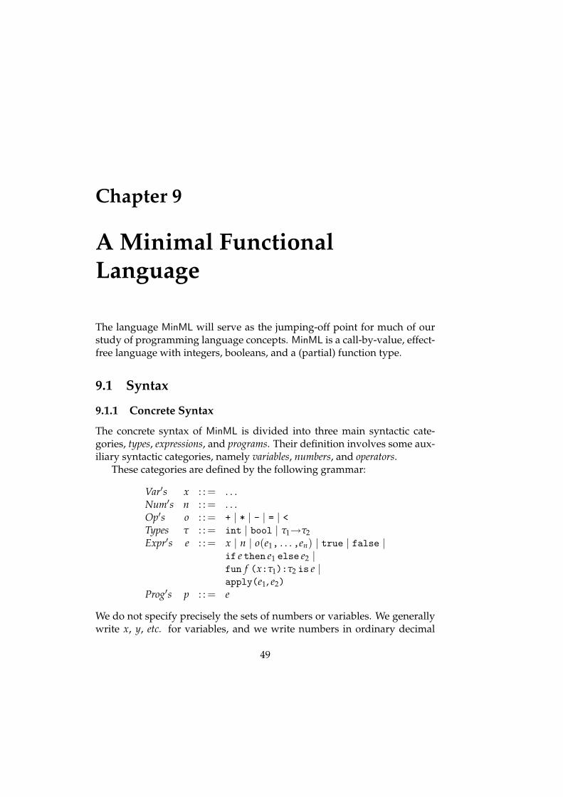
The concrete syntax of MinML is divided into three main syntactic cate-gories, types, expressions, and programs. Their definition involves some aux-iliary syntactic categories, namely variables, numbers, and operators.
These categories are defined by the following grammar:
Var′s x : : = . . .Num′s n : : = . . .Op′s o : : = + | * | - | = | <Types τ : : = int | bool | τ1→τ2Expr′s e : : = x | n | o(e1, . . . ,en) | true | false |
if e then e1 else e2 |fun f (x:τ1):τ2 is e |apply(e1, e2)
Prog′s p : : = e
We do not specify precisely the sets of numbers or variables. We generallywrite x, y, etc. for variables, and we write numbers in ordinary decimal
49

50 9.2 Static Semantics
notation. As usual we do not bother to specify such niceties as parenthe-sization or the use of infix syntax for binary operators, both of which wouldbe necessary in practice.
9.1.2 Abstract Syntax
The abstract syntax of MinML may be read off from its concrete syntax byinterpreting the preceding grammar as a specification of a set of abstractbinding trees, rather than as a set of strings. The only additional infor-mation we need, beyond what is provided by the context-free grammar, isa specification of the binding and scopes of names in an expression. In-formally, these may be specified by saying that in the function expressionfun f (x:τ1):τ2 is e the variables f and x are both bound within the bodyof the function, e. Written as an abt, a function expression has the formfun(τ1, τ2, f ,x.e), which has the virtue of making explicit that f and x arebound within e, and that the argument and result types of the function arepart of the syntax.
The following signature constitutes a precise definition of the abstractsyntax of MinML as a class of abt’s:
Operator Arityint ()bool ()→ (0, 0)
n ()o (0, . . . , 0︸ ︷︷ ︸
n
)
fun (0, 0, 2)apply (0, 0)true ()false ()if (0, 0, 0)
In the above specification o is an n-argument primitive operator.
9.2 Static Semantics
Not all expressions in MinML are sensible. For example, the expressionif 3 then 1 else 0 is not well-formed because 3 is an integer, whereas the
WORKING DRAFT SEPTEMBER 19, 2005

9.2 Static Semantics 51
conditional test expects a boolean. In other words, this expression is ill-typed because the expected constraint is not met. Expressions which dosatisfy these constraints are said to be well-typed, or well-formed.
Typing is clearly context-sensitive. The expression x + 3 may or maynot be well-typed, according to the type we assume for the variable x. Thatis, it depends on the surrounding context whether this sub-expression iswell-typed or not.
The three-place typing judgement, written Γ ` e : τ, states that e is a well-typed expression with type τ in the context Γ, which assigns types to somefinte set of names that may occur free in e. When e is closed (has no freevariables), we write simply e : τ instead of the more unwieldy ∅ ` e : τ.
We write Γ(x) for the unique type τ (if any) assigned to x by Γ. Thefunction Γ[x:τ], where x /∈ dom(Γ), is defined by the following equation
Γ[x:τ](y) =
τ if y = xΓ(y) otherwise
The typing relation is inductively defined by the following rules:
(Γ(x) = τ)Γ ` x : τ (9.1)
Here it is understood that if Γ(x) is undefined, then no type for x is deriv-able from assumptions Γ.
Γ ` n : int (9.2)
Γ ` true : bool (9.3)
Γ ` false : bool (9.4)
The typing rules for the arithmetic and boolean primitive operators are asexpected.
Γ ` e1 : int Γ ` e2 : intΓ ` +(e1, e2) : int (9.5)
Γ ` e1 : int Γ ` e2 : intΓ ` *(e1, e2) : int (9.6)
Γ ` e1 : int Γ ` e2 : intΓ ` -(e1, e2) : int (9.7)
SEPTEMBER 19, 2005 WORKING DRAFT
52 9.3 Properties of Typing
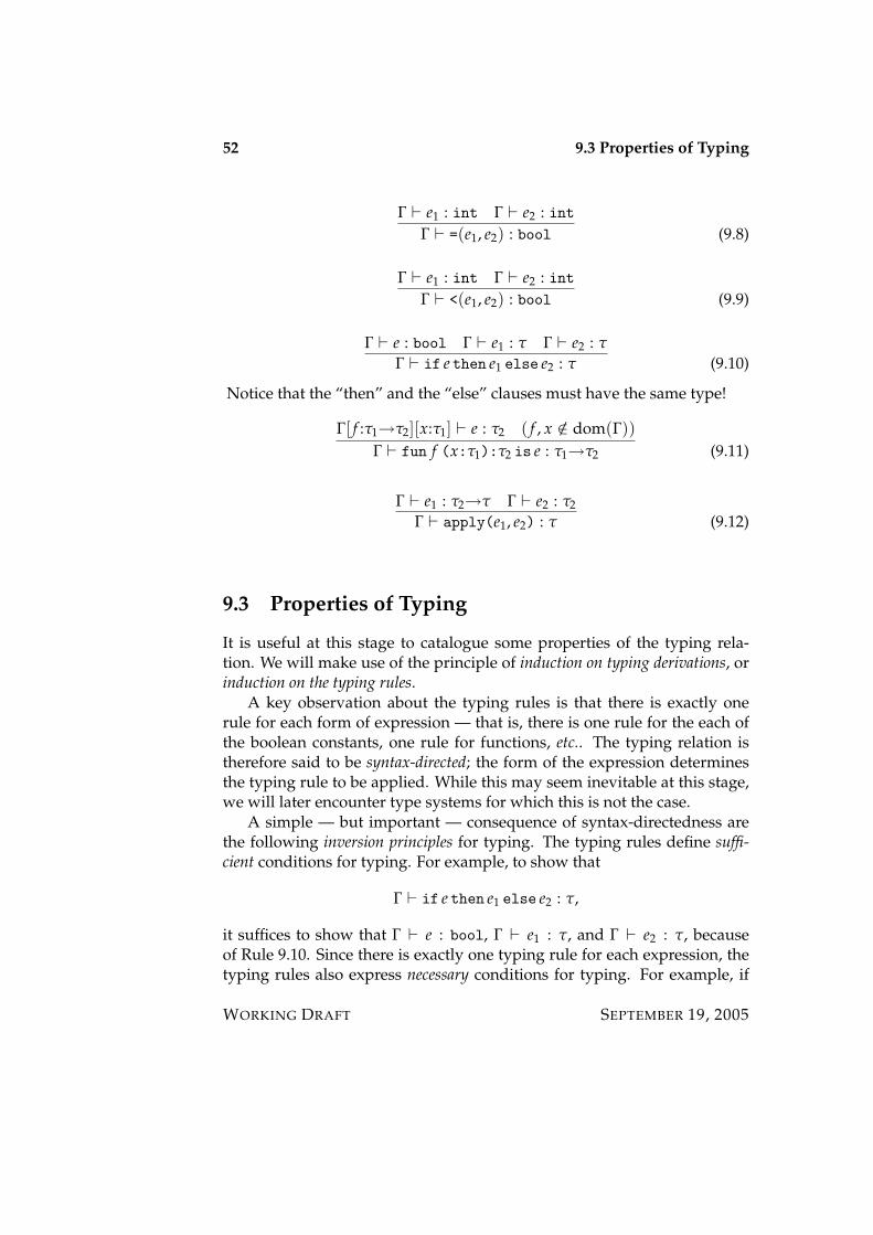
Γ ` e1 : int Γ ` e2 : intΓ ` =(e1, e2) : bool (9.8)
Γ ` e1 : int Γ ` e2 : intΓ ` <(e1, e2) : bool (9.9)
Γ ` e : bool Γ ` e1 : τ Γ ` e2 : τ
Γ ` if e then e1 else e2 : τ (9.10)
Notice that the “then” and the “else” clauses must have the same type!
Γ[ f :τ1→τ2][x:τ1] ` e : τ2 ( f , x /∈ dom(Γ))Γ ` fun f (x:τ1):τ2 is e : τ1→τ2 (9.11)
Γ ` e1 : τ2→τ Γ ` e2 : τ2
Γ ` apply(e1, e2) : τ (9.12)
9.3 Properties of Typing
It is useful at this stage to catalogue some properties of the typing rela-tion. We will make use of the principle of induction on typing derivations, orinduction on the typing rules.
A key observation about the typing rules is that there is exactly onerule for each form of expression — that is, there is one rule for the each ofthe boolean constants, one rule for functions, etc.. The typing relation istherefore said to be syntax-directed; the form of the expression determinesthe typing rule to be applied. While this may seem inevitable at this stage,we will later encounter type systems for which this is not the case.
A simple — but important — consequence of syntax-directedness arethe following inversion principles for typing. The typing rules define suffi-cient conditions for typing. For example, to show that
Γ ` if e then e1 else e2 : τ,
it suffices to show that Γ ` e : bool, Γ ` e1 : τ, and Γ ` e2 : τ, becauseof Rule 9.10. Since there is exactly one typing rule for each expression, thetyping rules also express necessary conditions for typing. For example, if
WORKING DRAFT SEPTEMBER 19, 2005
9.3 Properties of Typing 53
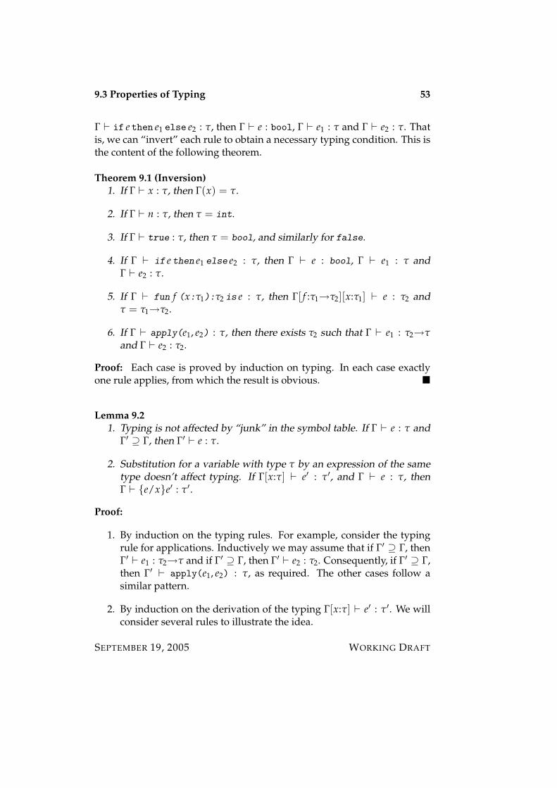
Γ ` if e then e1 else e2 : τ, then Γ ` e : bool, Γ ` e1 : τ and Γ ` e2 : τ. Thatis, we can “invert” each rule to obtain a necessary typing condition. This isthe content of the following theorem.
Theorem 9.1 (Inversion)1. If Γ ` x : τ, then Γ(x) = τ.
2. If Γ ` n : τ, then τ = int.
3. If Γ ` true : τ, then τ = bool, and similarly for false.
4. If Γ ` if e then e1 else e2 : τ, then Γ ` e : bool, Γ ` e1 : τ andΓ ` e2 : τ.
5. If Γ ` fun f (x:τ1):τ2 is e : τ, then Γ[ f :τ1→τ2][x:τ1] ` e : τ2 andτ = τ1→τ2.
6. If Γ ` apply(e1, e2) : τ, then there exists τ2 such that Γ ` e1 : τ2→τand Γ ` e2 : τ2.
Proof: Each case is proved by induction on typing. In each case exactlyone rule applies, from which the result is obvious.
Lemma 9.21. Typing is not affected by “junk” in the symbol table. If Γ ` e : τ and
Γ′ ⊇ Γ, then Γ′ ` e : τ.
2. Substitution for a variable with type τ by an expression of the sametype doesn’t affect typing. If Γ[x:τ] ` e′ : τ′, and Γ ` e : τ, thenΓ ` e/xe′ : τ′.
Proof:
1. By induction on the typing rules. For example, consider the typingrule for applications. Inductively we may assume that if Γ′ ⊇ Γ, thenΓ′ ` e1 : τ2→τ and if Γ′ ⊇ Γ, then Γ′ ` e2 : τ2. Consequently, if Γ′ ⊇ Γ,then Γ′ ` apply(e1, e2) : τ, as required. The other cases follow asimilar pattern.
2. By induction on the derivation of the typing Γ[x:τ] ` e′ : τ′. We willconsider several rules to illustrate the idea.
SEPTEMBER 19, 2005 WORKING DRAFT
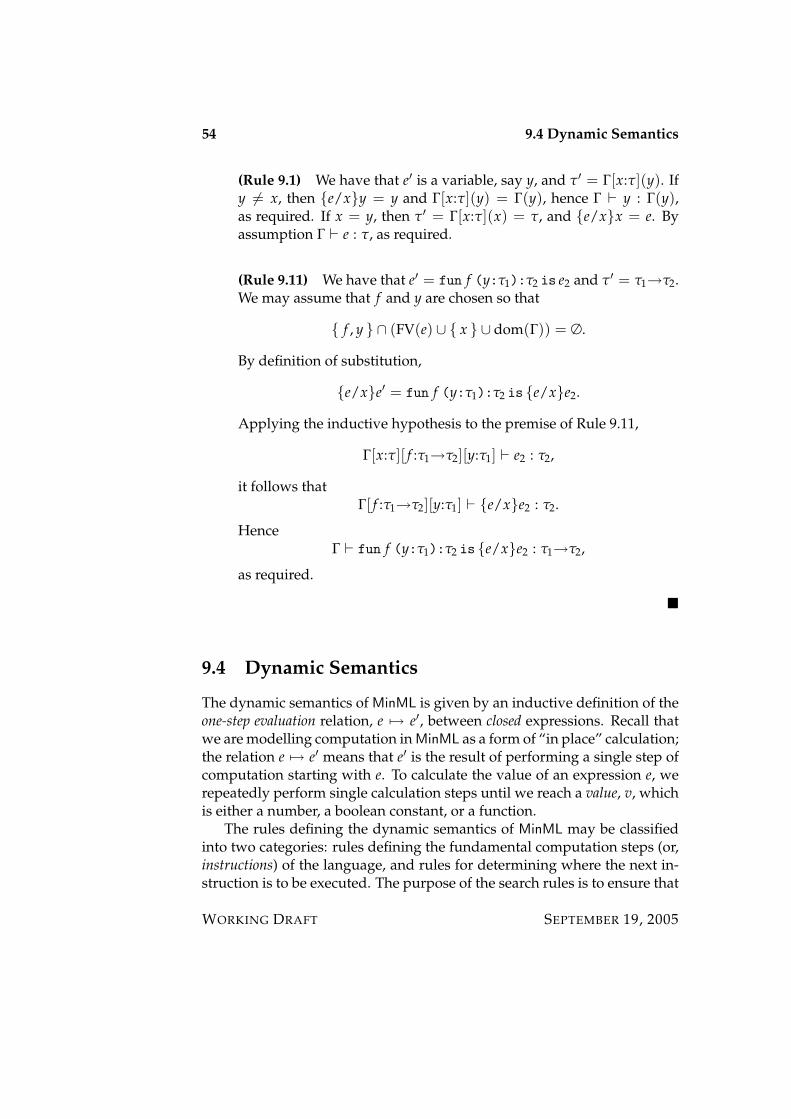
54 9.4 Dynamic Semantics
(Rule 9.1) We have that e′ is a variable, say y, and τ′ = Γ[x:τ](y). Ify 6= x, then e/xy = y and Γ[x:τ](y) = Γ(y), hence Γ ` y : Γ(y),as required. If x = y, then τ′ = Γ[x:τ](x) = τ, and e/xx = e. Byassumption Γ ` e : τ, as required.
(Rule 9.11) We have that e′ = fun f (y:τ1):τ2 is e2 and τ′ = τ1→τ2.We may assume that f and y are chosen so that
f , y ∩ (FV(e) ∪ x ∪ dom(Γ)) = ∅.
By definition of substitution,
e/xe′ = fun f (y:τ1):τ2 is e/xe2.
Applying the inductive hypothesis to the premise of Rule 9.11,
Γ[x:τ][ f :τ1→τ2][y:τ1] ` e2 : τ2,
it follows thatΓ[ f :τ1→τ2][y:τ1] ` e/xe2 : τ2.
HenceΓ ` fun f (y:τ1):τ2 is e/xe2 : τ1→τ2,
as required.
9.4 Dynamic Semantics
The dynamic semantics of MinML is given by an inductive definition of theone-step evaluation relation, e 7→ e′, between closed expressions. Recall thatwe are modelling computation in MinML as a form of “in place” calculation;the relation e 7→ e′ means that e′ is the result of performing a single step ofcomputation starting with e. To calculate the value of an expression e, werepeatedly perform single calculation steps until we reach a value, v, whichis either a number, a boolean constant, or a function.
The rules defining the dynamic semantics of MinML may be classifiedinto two categories: rules defining the fundamental computation steps (or,instructions) of the language, and rules for determining where the next in-struction is to be executed. The purpose of the search rules is to ensure that
WORKING DRAFT SEPTEMBER 19, 2005
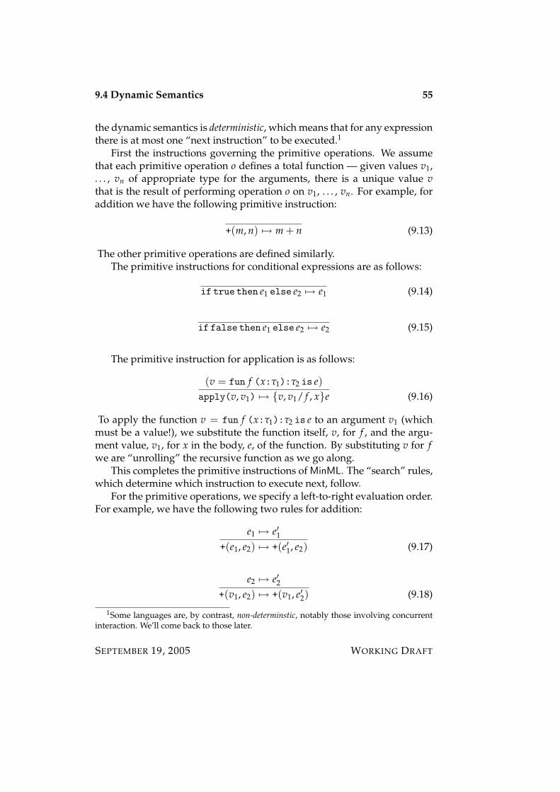
9.4 Dynamic Semantics 55
the dynamic semantics is deterministic, which means that for any expressionthere is at most one “next instruction” to be executed.1
First the instructions governing the primitive operations. We assumethat each primitive operation o defines a total function — given values v1,. . . , vn of appropriate type for the arguments, there is a unique value vthat is the result of performing operation o on v1, . . . , vn. For example, foraddition we have the following primitive instruction:
+(m, n) 7→ m + n (9.13)
The other primitive operations are defined similarly.The primitive instructions for conditional expressions are as follows:
if true then e1 else e2 7→ e1 (9.14)
if false then e1 else e2 7→ e2 (9.15)
The primitive instruction for application is as follows:
(v = fun f (x:τ1):τ2 is e)apply(v, v1) 7→ v, v1/ f , xe (9.16)
To apply the function v = fun f (x:τ1):τ2 is e to an argument v1 (whichmust be a value!), we substitute the function itself, v, for f , and the argu-ment value, v1, for x in the body, e, of the function. By substituting v for fwe are “unrolling” the recursive function as we go along.
This completes the primitive instructions of MinML. The “search” rules,which determine which instruction to execute next, follow.
For the primitive operations, we specify a left-to-right evaluation order.For example, we have the following two rules for addition:
e1 7→ e′1+(e1, e2) 7→ +(e′1, e2) (9.17)
e2 7→ e′2+(v1, e2) 7→ +(v1, e′2) (9.18)
1Some languages are, by contrast, non-determinstic, notably those involving concurrentinteraction. We’ll come back to those later.
SEPTEMBER 19, 2005 WORKING DRAFT
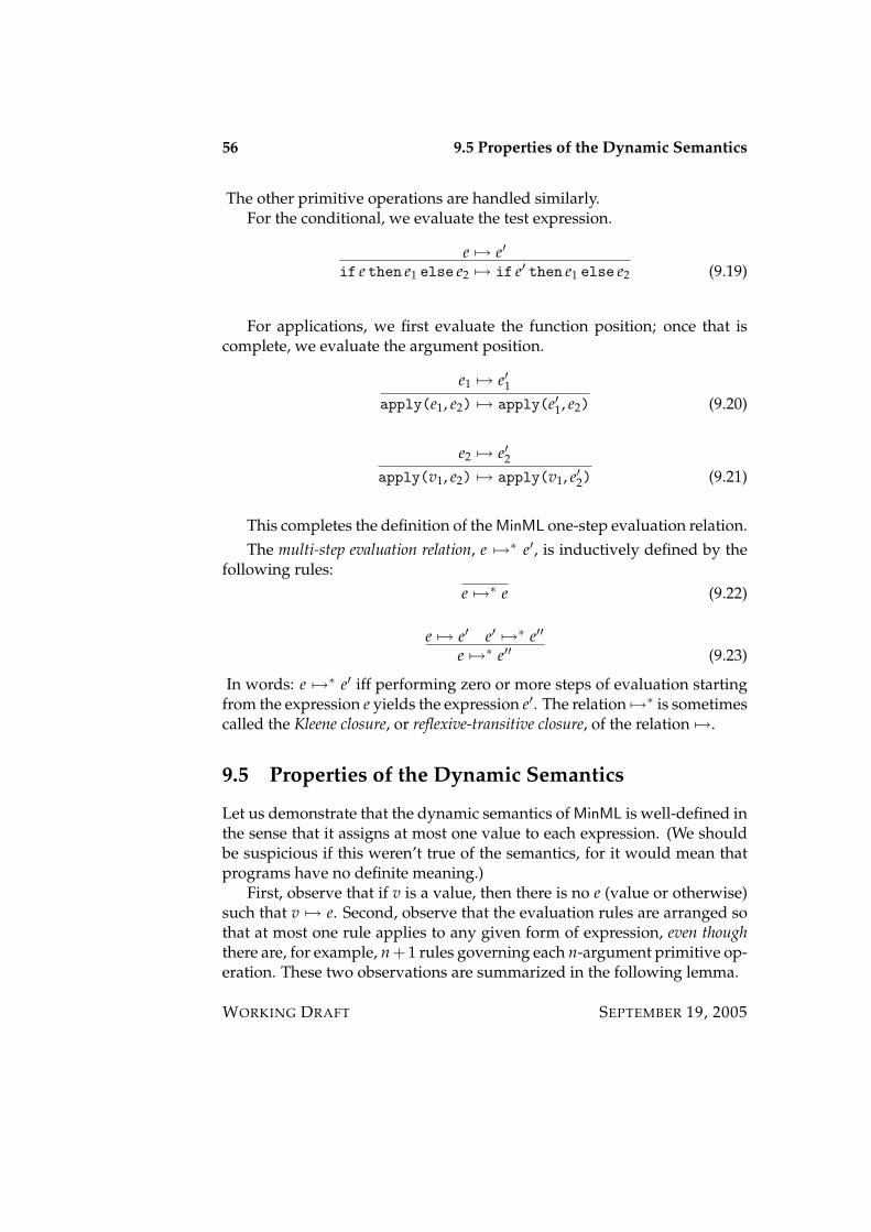
56 9.5 Properties of the Dynamic Semantics
The other primitive operations are handled similarly.For the conditional, we evaluate the test expression.
e 7→ e′
if e then e1 else e2 7→ if e′ then e1 else e2 (9.19)
For applications, we first evaluate the function position; once that iscomplete, we evaluate the argument position.
e1 7→ e′1apply(e1, e2) 7→ apply(e′1, e2) (9.20)
e2 7→ e′2apply(v1, e2) 7→ apply(v1, e′2) (9.21)
This completes the definition of the MinML one-step evaluation relation.The multi-step evaluation relation, e 7→∗ e′, is inductively defined by the
following rules:e 7→∗ e (9.22)
e 7→ e′ e′ 7→∗ e′′
e 7→∗ e′′ (9.23)
In words: e 7→∗ e′ iff performing zero or more steps of evaluation startingfrom the expression e yields the expression e′. The relation 7→∗ is sometimescalled the Kleene closure, or reflexive-transitive closure, of the relation 7→.
9.5 Properties of the Dynamic Semantics
Let us demonstrate that the dynamic semantics of MinML is well-defined inthe sense that it assigns at most one value to each expression. (We shouldbe suspicious if this weren’t true of the semantics, for it would mean thatprograms have no definite meaning.)
First, observe that if v is a value, then there is no e (value or otherwise)such that v 7→ e. Second, observe that the evaluation rules are arranged sothat at most one rule applies to any given form of expression, even thoughthere are, for example, n + 1 rules governing each n-argument primitive op-eration. These two observations are summarized in the following lemma.
WORKING DRAFT SEPTEMBER 19, 2005

9.6 Exercises 57
Lemma 9.3For every closed expression e, there exists at most one e′ such that e 7→ e′.In other words, the relation 7→ is a partial function.
Proof: By induction on the structure of e. We leave the proof as an exerciseto the reader. Be sure to consider all rules that apply to a given expressione!
It follows that evaluation to a value is deterministic:
Lemma 9.4For every closed expression e, there exists at most one value v such thate 7→∗ v.
Proof: Follows immediately from the preceding lemma, together with theobservation that there is no transition from a value.
9.6 Exercises
1. Can you think of a type system for a variant of MinML in which inver-sion fails? What form would such a type system have to take? Hint:think about overloading arithmetic operations.
2. Prove by induction on the structure of e that for every e and every Γthere exists at most one τ such that Γ ` e : τ. Hint: use rule inductionfor the rules defining the abstract syntax of expressions.
SEPTEMBER 19, 2005 WORKING DRAFT

58 9.6 Exercises
WORKING DRAFT SEPTEMBER 19, 2005
Chapter 10
Type Safety
Programming languages such as ML and Java are said to be “safe” (or,“type safe”, or “strongly typed”). Informally, this means that certain kindsof mismatches cannot arise during execution. For example, it will neverarise that an integer is to be applied to an argument, nor that two functionscould be added to each other. The goal of this section is to make this infor-mal notion precise. What is remarkable is that we will be able to clarify theidea of type safety without making reference to an implementation. Con-sequently, the notion of type safety is extremely robust — it is shared by allcorrect implementations of the language.
10.1 Defining Type Safety
Type safety is a relation between the static and dynamic semantics. It tellsus something about the execution of well-typed programs; it says nothingabout the execution of ill-typed programs. In implementation terms, we ex-pect ill-typed programs to be rejected by the compiler, so that nothing needbe said about their execution behavior (just as syntactically incorrect pro-grams are rejected, and nothing is said about what such a program mightmean).
In the framework we are developing, type safety amounts to the follow-ing two conditions:
1. Preservation. If e is a well-typed program, and e 7→ e′, then e′ is alsoa well-typed program.
2. Progress. If e is a well-typed program, then either e is a value, or thereexists e′ such that e 7→ e′.
59
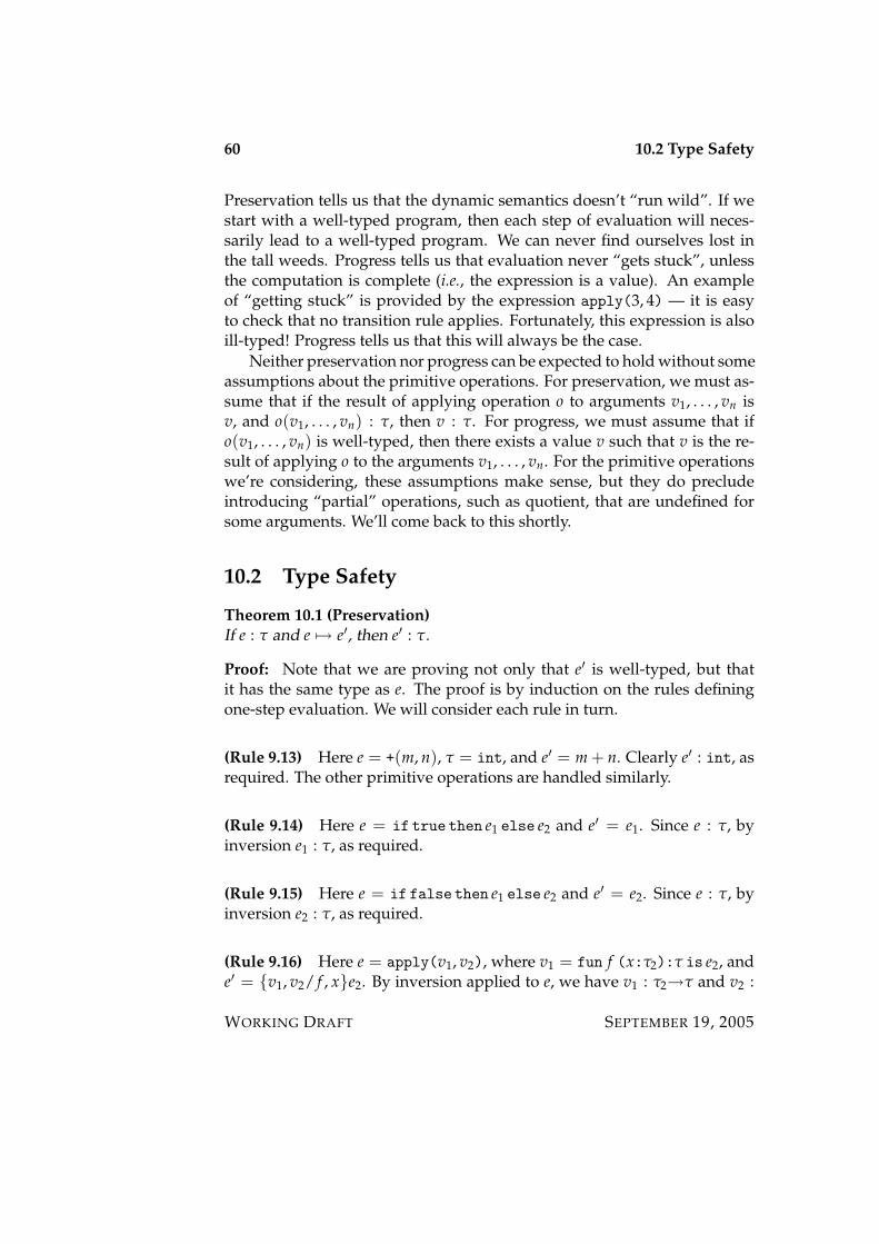
60 10.2 Type Safety
Preservation tells us that the dynamic semantics doesn’t “run wild”. If westart with a well-typed program, then each step of evaluation will neces-sarily lead to a well-typed program. We can never find ourselves lost inthe tall weeds. Progress tells us that evaluation never “gets stuck”, unlessthe computation is complete (i.e., the expression is a value). An exampleof “getting stuck” is provided by the expression apply(3, 4) — it is easyto check that no transition rule applies. Fortunately, this expression is alsoill-typed! Progress tells us that this will always be the case.
Neither preservation nor progress can be expected to hold without someassumptions about the primitive operations. For preservation, we must as-sume that if the result of applying operation o to arguments v1, . . . , vn isv, and o(v1, . . . , vn) : τ, then v : τ. For progress, we must assume that ifo(v1, . . . , vn) is well-typed, then there exists a value v such that v is the re-sult of applying o to the arguments v1, . . . , vn. For the primitive operationswe’re considering, these assumptions make sense, but they do precludeintroducing “partial” operations, such as quotient, that are undefined forsome arguments. We’ll come back to this shortly.
10.2 Type Safety
Theorem 10.1 (Preservation)If e : τ and e 7→ e′, then e′ : τ.
Proof: Note that we are proving not only that e′ is well-typed, but thatit has the same type as e. The proof is by induction on the rules definingone-step evaluation. We will consider each rule in turn.
(Rule 9.13) Here e = +(m, n), τ = int, and e′ = m + n. Clearly e′ : int, asrequired. The other primitive operations are handled similarly.
(Rule 9.14) Here e = if true then e1 else e2 and e′ = e1. Since e : τ, byinversion e1 : τ, as required.
(Rule 9.15) Here e = if false then e1 else e2 and e′ = e2. Since e : τ, byinversion e2 : τ, as required.
(Rule 9.16) Here e = apply(v1, v2), where v1 = fun f (x:τ2):τ is e2, ande′ = v1, v2/ f , xe2. By inversion applied to e, we have v1 : τ2→τ and v2 :
WORKING DRAFT SEPTEMBER 19, 2005
10.2 Type Safety 61
τ2. By inversion applied to v1, we have [ f :τ2→τ][x:τ2] ` e2 : τ. Therefore,by substitution we have v1, v2/ f , xe2 : τ, as required.
(Rule 9.17) Here e = +(e1, e2), e′ = +(e′1, e2), and e1 7→ e′1. By inversione1 : int, so that by induction e′1 : int, and hence e′ : int, as required.
(Rule 9.18) Here e = +(v1, e2), e′ = +(v1, e′2), and e2 7→ e′2. By inversione2 : int, so that by induction e′2 : int, and hence e′ : int, as required.
The other primitive operations are handled similarly.
(Rule 9.19) Here e = if e1 then e2 else e3 and e′ = if e′1 then e2 else e3.By inversion we have that e1 : bool, e2 : τ and e3 : τ. By inductive hypoth-esis e′1 : bool, and hence e′ : τ.
(Rule 9.20) Here e = apply(e1, e2) and e′ = apply(e′1, e2). By inversione1 : τ2→τ and e2 : τ2, for some type τ2. By induction e′1 : τ2→τ, and hencee′ : τ.
(Rule 9.21) Here e = apply(v1, e2) and e′ = apply(v1, e′2). By inversion,v1 : τ2→τ and e2 : τ2, for some type τ2. By induction e′2 : τ2, and hencee′ : τ.
The type of a closed value “predicts” its form.
Lemma 10.2 (Canonical Forms)Suppose that v : τ is a closed, well-formed value.
1. If τ = bool, then either v = true or v = false.
2. If τ = int, then v = n for some n.
3. If τ = τ1→τ2, then v = fun f (x:τ1):τ2 is e for some f , x, and e.
Proof: By induction on the typing rules, using the fact that v is a value.
Exercise 10.3Give a proof of the canonical forms lemma.
SEPTEMBER 19, 2005 WORKING DRAFT
62 10.2 Type Safety
Theorem 10.4 (Progress)If e : τ, then either e is a value, or there exists e′ such that e 7→ e′.
Proof: The proof is by induction on the typing rules.
(Rule 9.1) Cannot occur, since e is closed.
(Rules 9.2, 9.3, 9.4, 9.11) In each case e is a value, which completes theproof.
(Rule 9.5) Here e = +(e1, e2) and τ = int, with e1 : int and e2 : int. Byinduction we have either e1 is a value, or there exists e′1 such that e1 7→ e′1for some expression e′1. In the latter case it follows that e 7→ e′, wheree′ = +(e′1, e2). In the former case, we note that by the canonical forms lemmae1 = n1 for some n1, and we consider e2. By induction either e2 is a value, ore2 7→ e′2 for some expression e′2. If e2 is a value, then by the canonical formslemma e2 = n2 for some n2, and we note that e 7→ e′, where e′ = n1 + n2.Otherwise, e 7→ e′, where e′ = +(v1, e′2), as desired.
(Rule 9.10) Here e = if e1 then e2 else e3, with e1 : bool, e2 : τ, and e3 :τ. By the first inductive hypothesis, either e1 is a value, or there exists e′1such that e1 7→ e′1. If e1 is a value, then we have by the Canonical FormsLemma, either e1 = true or e1 = false. In the former case e 7→ e2, andin the latter e 7→ e3, as required. If e1 is not a value, then e 7→ e′, wheree′ = if e′1 then e2 else e3, by Rule 9.19.
(Rule 9.12) Here e = apply(e1, e2), with e1 : τ2→τ and e2 : τ2. By the firstinductive hypothesis, either e1 is a value, or there exists e′1 such that e1 7→ e′1.If e1 is not a value, then e 7→ apply(e′1, e2) by Rule 9.20, as required. By thesecond inductive hypothesis, either e2 is a value, or there exists e′2 such thate2 7→ e′2. If e2 is not a value, then e 7→ e′, where e′ = apply(e1, e′2), asrequired. Finally, if both e1 and e2 are values, then by the Canonical FormsLemma, e1 = fun f (x:τ2):τ is e′′, and e 7→ e′, where e′ = e1, e2/ f , xe′′,by Rule 9.16.
Theorem 10.5 (Safety)If e is closed and well-typed, then evaluation of e can only terminate witha value of the same type. In particular, evaluation cannot “get stuck” in an
WORKING DRAFT SEPTEMBER 19, 2005
10.3 Run-Time Errors and Safety 63
ill-defined state.
10.3 Run-Time Errors and Safety
Stuck states correspond to ill-defined programs that attempt to, say, treatan integer as a pointer to a function, or that move a pointer beyond thelimits of a region of memory. In an unsafe language there are no stuck states— every program will do something — but it may be impossible to predicthow the program will behave in certain situations. It may “dump core”, orit may allow the programmer to access private data, or it may compute a“random” result.
The best-known example of an unsafe language is C. It’s lack of safetymanifests itself in numerous ways, notably in that computer viruses nearlyalways rely on overrunning a region of memory as a critical step in an at-tack. Another symptom is lack of portability: an unsafe program may ex-ecute sensibly on one platform, but behave entirely differently on another.To avoid this behavior, standards bodies have defined portable subsets ofC that are guaranteed to have predictable behavior on all platforms. Butthere is no good way to ensure that a programmer, whether through maliceor neglect, adheres to this subset.1
Safe languages, in contrast, avoid ill-defined states entirely, by imposingtyping restrictions that ensure that well-typed programs have well-definedbehavior. MinML is a good example of a safe language. It is inherentlyportable, because its dynamic semantics is specified in an implementation-independent manner, and because its static semantics ensures that well-typed programs never “get stuck”. Stated contrapositively, the type safetytheorem for MinML assures us that stuck states are ill-typed.
But suppose that we add to MinML a primitive operation, such as quo-tient, that is undefined for certain arguments. An expression such as 3/0would most-assuredly be “stuck”, yet would be well-typed, at least if wetake the natural typing rule for it:
Γ ` e1 : int Γ ` e2 : intΓ ` e1 / e2 : int
What are we to make of this? Is the extension of MinML with quotientunsafe?
To recover safety, we have two options:
1It should be easy to convince yourself that it is undecidable whether a given C programcan reach an implementation-dependent state.
SEPTEMBER 19, 2005 WORKING DRAFT
64 10.3 Run-Time Errors and Safety
1. Enhance the type system so that no well-typed program can ever divideby zero.
2. Modify the dynamic semantics so that division by zero is not “stuck”,but rather incurs a run-time error.
The first option amounts to requiring that the type checker prove that thedenominator of a quotient is non-zero in order for it to be well-typed. Butthis means that the type system would, in general, be undecidable, for wecan easily arrange for the denominator of some expression to be non-zeroexactly when some Turing machine halts on blank tape. It is the subject ofongoing research to devise conservative type checkers that are sufficientlyexpressive to be useful in practice, but we shall not pursue this approachany further here.
The second option is widely used. It is based on distinguishing checkedfrom unchecked errors. A checked error is one that is detected at executiontime by an explicit test for ill-defined situations. For example, the quotientoperation tests whether its denominator is zero, incurring an error if so. Anunchecked error is one that is not detected at execution time, but rather isregarded as “stuck” or “ill-defined”. Type errors in MinML are uncheckederrors, precisely because the static semantics ensures that they can neveroccur.
The point of introducing checked errors is that they ensure well-definedbehavior even for ill-defined programs. Thus 3/0 evaluates to error, ratherthan simply “getting stuck” or behaving unpredictably. The essence of typesafety is that well-typed programs should have well-defined behavior, evenif that behavior is to signal an error. That way we can predict how the pro-gram will behave simply by looking at the program itself, without regard tothe implementation or platform. In this sense safe languages are inherentlyportable, which explains the recent resurgence in interest in them.
How might checked errors be added to MinML? The main idea is to addto MinML a special expression, error, that designates a run-time fault in anexpression. Its typing rule is as follows:
Γ ` error : τ (10.1)
Note that a run-time error can have any type at all. The reasons for thiswill become clear once we re-state the safety theorem.
The dynamic semantics is augmented in two ways. First, we add newtransitions for the checked errors. For example, the following rule checks
WORKING DRAFT SEPTEMBER 19, 2005
10.3 Run-Time Errors and Safety 65
for a zero denominator in a quotient:
v1 / 0 7→ error (10.2)
Second, we add rules to propagate errors; once an error has arisen, it abortsthe rest of the computation. Here are two representative error propagationrules:
apply(error, v2) 7→ error (10.3)
apply(v1, error) 7→ error (10.4)
These rule state that if the function or argument position of an applicationincur an error, then so does the entire application.
With these changes, the type safety theorem may be stated as follows:
Theorem 10.6 (Safety With Errors)If an expression is well-typed, it can only evaluate to a value or evaluate toerror. It cannot “get stuck” in an ill-defined state.
As before, safety follows from preservation and progress. The preser-vation theorem states that types are preserved by evaluation. We have al-ready proved this for MinML; we need only consider error transitions. Butfor these preservation is trivial, since error has any type whatsoever. Thecanonical forms lemma carries over without change. The progress theoremis proved as before, relying on checked errors to ensure that progress canbe made, even in ill-defined states such as division by zero.
SEPTEMBER 19, 2005 WORKING DRAFT
66 10.3 Run-Time Errors and Safety
WORKING DRAFT SEPTEMBER 19, 2005
Part IV
Control and Data Flow
67

Chapter 11
Abstract Machines
Long considered to be a topic of primarily academic interest, abstract, or vir-tual, machines are now attracting renewed attention, especially by the soft-ware industry. The main idea is to define an instruction set for a “pseudo-computer”, the abstract machine, that may be used as the object code forcompiling a high-level language (such as ML or Java) and that may be im-plemented with reasonable efficiency on a wide variety of stock platforms.This means that the high-level language must be implemented only once,for the abstract machine, but that the abstract machine must itself be im-plemented once per platform. One advantage is that it is, in principle,much easier to port the abstract machine than it is to re-implement thelanguage for each platform. More importantly, this architecture supportsthe exchange of object code across the network — if everyone implementsthe abstract machine, then code can migrate from one computer to anotherwithout modification. Web sites all over the world exploit this capability totremendous advantage, using the Java Virtual Machine.
Before we get started, let us ask ourselves the question: what is an ab-stract machine? In other words, what is a computer? The fundamental ideaof computation is the notion of step-by-step execution of instructions thattransform the state of the computer in some determinate fashion.1 Eachinstruction should be executable in a finite amount of time using a finiteamount of information, and it should be clear how to effect the requiredstate transformation using only physically realizable methods.2 Execution
1The question of determinacy is increasingly problematic for real computers, largelybecause of the aggressive use of parallelism in their implementation. We will gloss overthis issue here.
2For example, consider the instruction that, given the representation of a program, setsregister zero to one iff there is an input on which that program halts when executed, and
69
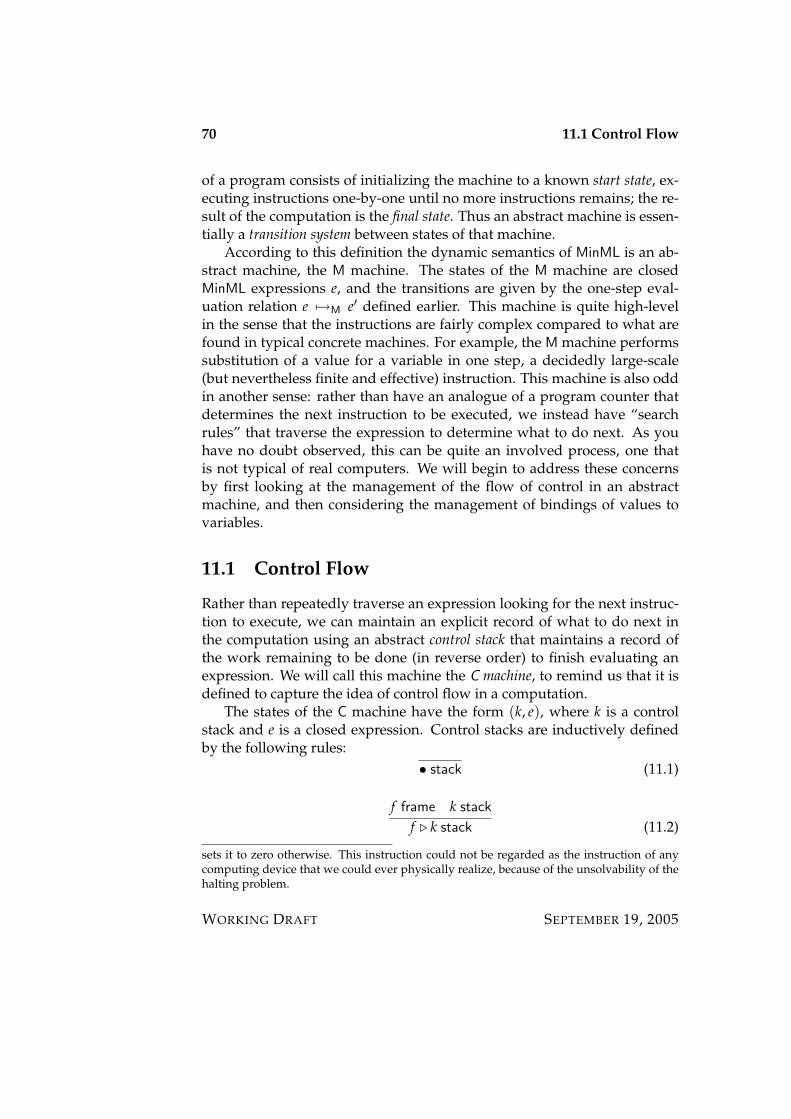
70 11.1 Control Flow
of a program consists of initializing the machine to a known start state, ex-ecuting instructions one-by-one until no more instructions remains; the re-sult of the computation is the final state. Thus an abstract machine is essen-tially a transition system between states of that machine.
According to this definition the dynamic semantics of MinML is an ab-stract machine, the M machine. The states of the M machine are closedMinML expressions e, and the transitions are given by the one-step eval-uation relation e 7→M e′ defined earlier. This machine is quite high-levelin the sense that the instructions are fairly complex compared to what arefound in typical concrete machines. For example, the M machine performssubstitution of a value for a variable in one step, a decidedly large-scale(but nevertheless finite and effective) instruction. This machine is also oddin another sense: rather than have an analogue of a program counter thatdetermines the next instruction to be executed, we instead have “searchrules” that traverse the expression to determine what to do next. As youhave no doubt observed, this can be quite an involved process, one thatis not typical of real computers. We will begin to address these concernsby first looking at the management of the flow of control in an abstractmachine, and then considering the management of bindings of values tovariables.
11.1 Control Flow
Rather than repeatedly traverse an expression looking for the next instruc-tion to execute, we can maintain an explicit record of what to do next inthe computation using an abstract control stack that maintains a record ofthe work remaining to be done (in reverse order) to finish evaluating anexpression. We will call this machine the C machine, to remind us that it isdefined to capture the idea of control flow in a computation.
The states of the C machine have the form (k, e), where k is a controlstack and e is a closed expression. Control stacks are inductively definedby the following rules:
• stack (11.1)
f frame k stack
f . k stack (11.2)
sets it to zero otherwise. This instruction could not be regarded as the instruction of anycomputing device that we could ever physically realize, because of the unsolvability of thehalting problem.
WORKING DRAFT SEPTEMBER 19, 2005
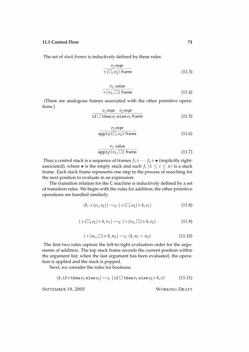
11.1 Control Flow 71
The set of stack frames is inductively defined by these rules:
e2 expr
+(, e2) frame (11.3)
v1 value
+(v1,) frame (11.4)
(There are analogous frames associated with the other primitive opera-tions.)
e1 expr e2 expr
if then e1 else e2 frame (11.5)
e2 expr
apply(, e2) frame (11.6)
v1 value
apply(v1,) frame (11.7)
Thus a control stack is a sequence of frames f1 . · · · fn . • (implicitly right-associated), where • is the empty stack and each fi (1 ≤ i ≤ n) is a stackframe. Each stack frame represents one step in the process of searching forthe next position to evaluate in an expression.
The transition relation for the C machine is inductively defined by a setof transition rules. We begin with the rules for addition; the other primitiveoperations are handled similarly.
(k, +(e1, e2)) 7→C (+(, e2) . k, e1) (11.8)
(+(, e2) . k, v1) 7→C (+(v1,) . k, e2) (11.9)
(+(n1,) . k, n2) 7→C (k, n1 + n2) (11.10)
The first two rules capture the left-to-right evaluation order for the argu-ments of addition. The top stack frame records the current position withinthe argument list; when the last argument has been evaluated, the opera-tion is applied and the stack is popped.
Next, we consider the rules for booleans.
(k, if e then e1 else e2) 7→C (if then e1 else e2 . k, e) (11.11)
SEPTEMBER 19, 2005 WORKING DRAFT
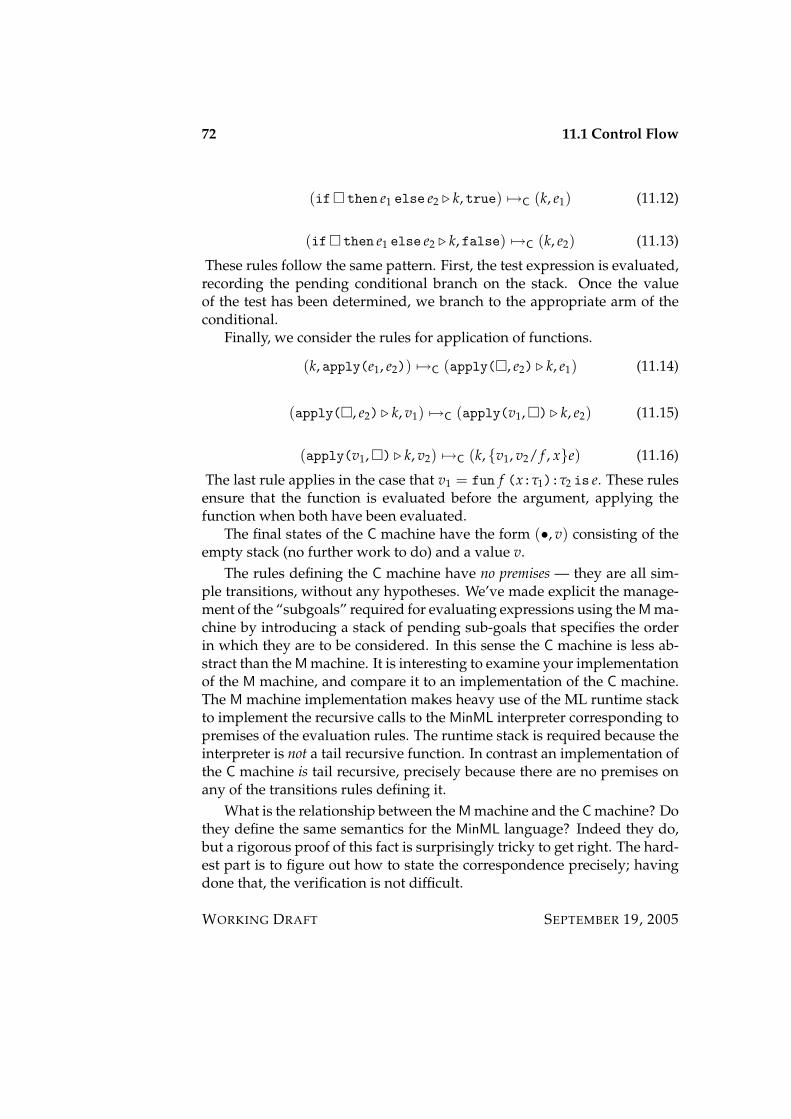
72 11.1 Control Flow
(if then e1 else e2 . k, true) 7→C (k, e1) (11.12)
(if then e1 else e2 . k, false) 7→C (k, e2) (11.13)
These rules follow the same pattern. First, the test expression is evaluated,recording the pending conditional branch on the stack. Once the valueof the test has been determined, we branch to the appropriate arm of theconditional.
Finally, we consider the rules for application of functions.
(k, apply(e1, e2)) 7→C (apply(, e2) . k, e1) (11.14)
(apply(, e2) . k, v1) 7→C (apply(v1,) . k, e2) (11.15)
(apply(v1,) . k, v2) 7→C (k, v1, v2/ f , xe) (11.16)
The last rule applies in the case that v1 = fun f (x:τ1):τ2 is e. These rulesensure that the function is evaluated before the argument, applying thefunction when both have been evaluated.
The final states of the C machine have the form (•, v) consisting of theempty stack (no further work to do) and a value v.
The rules defining the C machine have no premises — they are all sim-ple transitions, without any hypotheses. We’ve made explicit the manage-ment of the “subgoals” required for evaluating expressions using the M ma-chine by introducing a stack of pending sub-goals that specifies the orderin which they are to be considered. In this sense the C machine is less ab-stract than the M machine. It is interesting to examine your implementationof the M machine, and compare it to an implementation of the C machine.The M machine implementation makes heavy use of the ML runtime stackto implement the recursive calls to the MinML interpreter corresponding topremises of the evaluation rules. The runtime stack is required because theinterpreter is not a tail recursive function. In contrast an implementation ofthe C machine is tail recursive, precisely because there are no premises onany of the transitions rules defining it.
What is the relationship between the M machine and the C machine? Dothey define the same semantics for the MinML language? Indeed they do,but a rigorous proof of this fact is surprisingly tricky to get right. The hard-est part is to figure out how to state the correspondence precisely; havingdone that, the verification is not difficult.
WORKING DRAFT SEPTEMBER 19, 2005
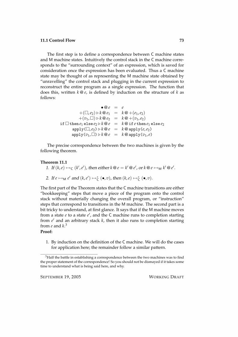
11.1 Control Flow 73
The first step is to define a correspondence between C machine statesand M machine states. Intuitively the control stack in the C machine corre-sponds to the “surrounding context” of an expression, which is saved forconsideration once the expression has been evaluated. Thus a C machinestate may be thought of as representing the M machine state obtained by“unravelling” the control stack and plugging in the current expression toreconstruct the entire program as a single expression. The function thatdoes this, written k @ e, is defined by induction on the structure of k asfollows:
•@ e = e+(, e2) . k @ e1 = k @ +(e1, e2)+(v1,) . k @ e2 = k @ +(v1, e2)
if then e1 else e2 . k @ e = k @ if e then e1 else e2apply(, e2) . k @ e = k @ apply(e, e2)apply(v1,) . k @ e = k @ apply(v1, e)
The precise correspondence between the two machines is given by thefollowing theorem.
Theorem 11.11. If (k, e) 7→C (k′, e′), then either k @ e = k′ @ e′, or k @ e 7→M k′ @ e′.
2. If e 7→M e′ and (k, e′) 7→∗C (•, v), then (k, e) 7→∗C (•, v).
The first part of the Theorem states that the C machine transitions are either“bookkeeping” steps that move a piece of the program onto the controlstack without materially changing the overall program, or “instruction”steps that correspond to transitions in the M machine. The second part is abit tricky to understand, at first glance. It says that if the M machine movesfrom a state e to a state e′, and the C machine runs to completion startingfrom e′ and an arbitrary stack k, then it also runs to completion startingfrom e and k.3
Proof:
1. By induction on the definition of the C machine. We will do the casesfor application here; the remainder follow a similar pattern.
3Half the battle in establishing a correspondence between the two machines was to findthe proper statement of the correspondence! So you should not be dismayed if it takes sometime to understand what is being said here, and why.
SEPTEMBER 19, 2005 WORKING DRAFT

74 11.1 Control Flow
(a) Consider the transition
(k, apply(e1, e2)) 7→C (apply(, e2) . k, e1).
Here e = apply(e1, e2), k′ = apply(, e2) . k, and e′ = e1. It iseasy to check that k @ e = k′ @ e′.
(b) Consider the transition
(apply(, e2) . k′′, v1) 7→C (apply(v1,) . k′′, e2).
Here e = v1, k = apply(, e2). k′′, e′ = e2, and k′ = apply(v1,).k′′. It is easy to check that k @ e = k′ @ e′.
(c) Consider the transition
(apply(v1,) . k′, v2) 7→C (k′, v1, v2/ f , xe),
where v1 = fun f (x:τ2):τ is e. Here k = apply(v1,) . k′,e = v2, and e′ = v1, v2/ f , xe. We have
k @ e = k′ @ apply(v1, v2)7→ k′ @ e′
as desired. The second step follows from the observation thatstacks are defined so that the M search rules “glide over” k′ —the next instruction to execute in k′ @ apply(v1, v2) must be theapplication apply(v1, v2).
2. By induction on the MinML dynamic semantics. We will do the casesfor application here; the remainder follow a similar pattern.
(a) e = apply(v1, v2) 7→M v1, v2/ f , xe2 = e′, where the valuev1 = fun f (x:τ2):τ is e2. Suppose that (k, e′) 7→∗C (•, v). By thedefinition of the C machine transition relation,
(k, e) 7→C (apply(, v2) . k, v1)7→C (apply(v1,) . k, v2)7→C (k, e′)
From this, the result follows immediately.
(b) e = apply(e1, e2) 7→M apply(e′1, e2) = e′, where e1 7→M e′1. Sup-pose that (k, e′) 7→∗C (•, v). Since e′ = apply(e′1, e2), and since the
WORKING DRAFT SEPTEMBER 19, 2005
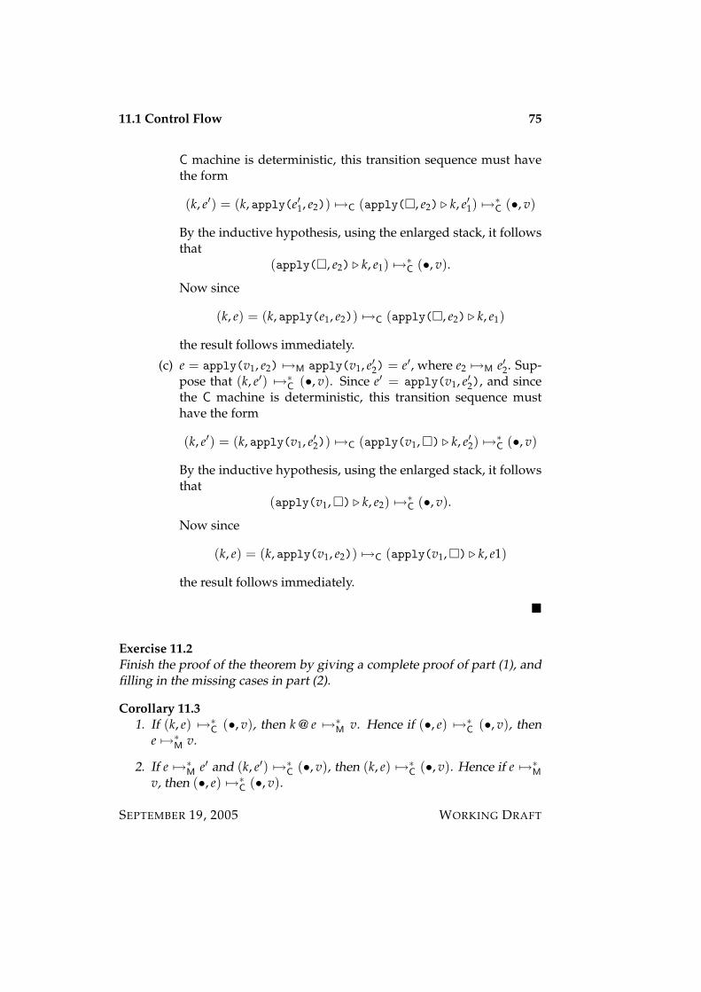
11.1 Control Flow 75
C machine is deterministic, this transition sequence must havethe form
(k, e′) = (k, apply(e′1, e2)) 7→C (apply(, e2) . k, e′1) 7→∗C (•, v)
By the inductive hypothesis, using the enlarged stack, it followsthat
(apply(, e2) . k, e1) 7→∗C (•, v).
Now since
(k, e) = (k, apply(e1, e2)) 7→C (apply(, e2) . k, e1)
the result follows immediately.
(c) e = apply(v1, e2) 7→M apply(v1, e′2) = e′, where e2 7→M e′2. Sup-pose that (k, e′) 7→∗C (•, v). Since e′ = apply(v1, e′2), and sincethe C machine is deterministic, this transition sequence musthave the form
(k, e′) = (k, apply(v1, e′2)) 7→C (apply(v1,) . k, e′2) 7→∗C (•, v)
By the inductive hypothesis, using the enlarged stack, it followsthat
(apply(v1,) . k, e2) 7→∗C (•, v).
Now since
(k, e) = (k, apply(v1, e2)) 7→C (apply(v1,) . k, e1)
the result follows immediately.
Exercise 11.2Finish the proof of the theorem by giving a complete proof of part (1), andfilling in the missing cases in part (2).
Corollary 11.31. If (k, e) 7→∗C (•, v), then k @ e 7→∗M v. Hence if (•, e) 7→∗C (•, v), then
e 7→∗M v.
2. If e 7→∗M e′ and (k, e′) 7→∗C (•, v), then (k, e) 7→∗C (•, v). Hence if e 7→∗Mv, then (•, e) 7→∗C (•, v).
SEPTEMBER 19, 2005 WORKING DRAFT
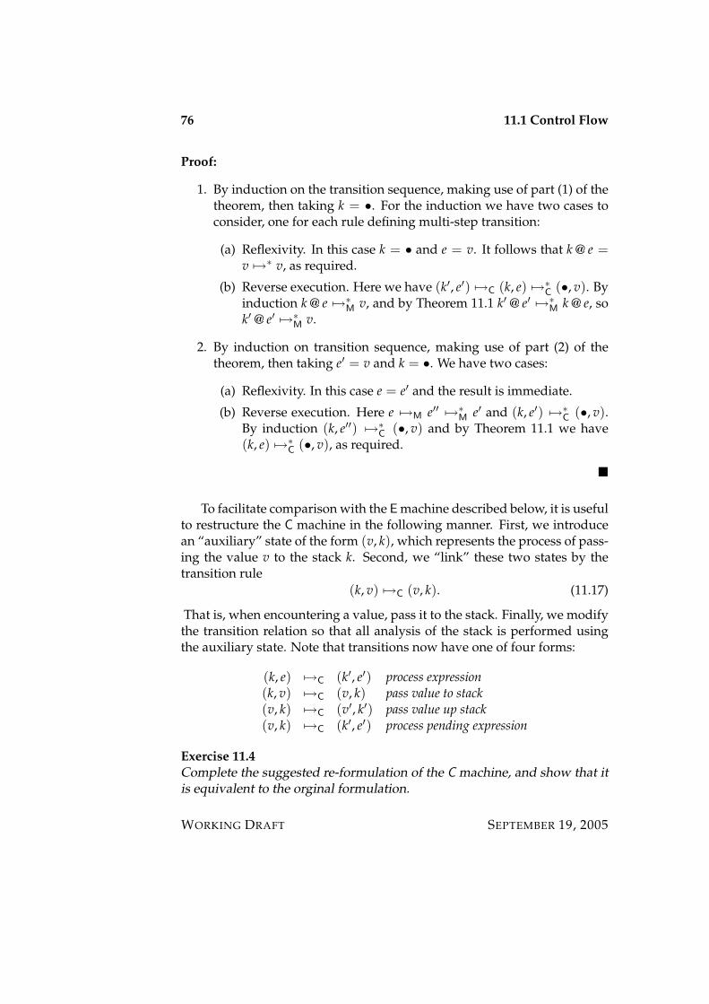
76 11.1 Control Flow
Proof:
1. By induction on the transition sequence, making use of part (1) of thetheorem, then taking k = •. For the induction we have two cases toconsider, one for each rule defining multi-step transition:
(a) Reflexivity. In this case k = • and e = v. It follows that k @ e =v 7→∗ v, as required.
(b) Reverse execution. Here we have (k′, e′) 7→C (k, e) 7→∗C (•, v). Byinduction k @ e 7→∗M v, and by Theorem 11.1 k′ @ e′ 7→∗M k @ e, sok′ @ e′ 7→∗M v.
2. By induction on transition sequence, making use of part (2) of thetheorem, then taking e′ = v and k = •. We have two cases:
(a) Reflexivity. In this case e = e′ and the result is immediate.
(b) Reverse execution. Here e 7→M e′′ 7→∗M e′ and (k, e′) 7→∗C (•, v).By induction (k, e′′) 7→∗C (•, v) and by Theorem 11.1 we have(k, e) 7→∗C (•, v), as required.
To facilitate comparison with the E machine described below, it is usefulto restructure the C machine in the following manner. First, we introducean “auxiliary” state of the form (v, k), which represents the process of pass-ing the value v to the stack k. Second, we “link” these two states by thetransition rule
(k, v) 7→C (v, k). (11.17)
That is, when encountering a value, pass it to the stack. Finally, we modifythe transition relation so that all analysis of the stack is performed usingthe auxiliary state. Note that transitions now have one of four forms:
(k, e) 7→C (k′, e′) process expression(k, v) 7→C (v, k) pass value to stack(v, k) 7→C (v′, k′) pass value up stack(v, k) 7→C (k′, e′) process pending expression
Exercise 11.4Complete the suggested re-formulation of the C machine, and show that itis equivalent to the orginal formulation.
WORKING DRAFT SEPTEMBER 19, 2005
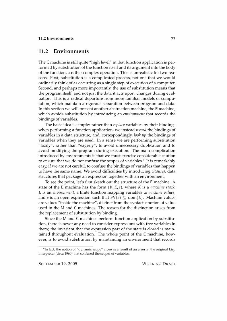
11.2 Environments 77
11.2 Environments
The C machine is still quite “high level” in that function application is per-formed by substitution of the function itself and its argument into the bodyof the function, a rather complex operation. This is unrealistic for two rea-sons. First, substitution is a complicated process, not one that we wouldordinarily think of as occurring as a single step of execution of a computer.Second, and perhaps more importantly, the use of substitution means thatthe program itself, and not just the data it acts upon, changes during eval-uation. This is a radical departure from more familiar models of compu-tation, which maintain a rigorous separation between program and data.In this section we will present another abstraction machine, the E machine,which avoids substitution by introducing an environment that records thebindings of variables.
The basic idea is simple: rather than replace variables by their bindingswhen performing a function application, we instead record the bindings ofvariables in a data structure, and, correspondingly, look up the bindings ofvariables when they are used. In a sense we are performing substitution“lazily”, rather than “eagerly”, to avoid unnecessary duplication and toavoid modifying the program during execution. The main complicationintroduced by environments is that we must exercise considerable cautionto ensure that we do not confuse the scopes of variables.4 It is remarkablyeasy, if we are not careful, to confuse the bindings of variables that happento have the same name. We avoid difficulties by introducing closures, datastructures that package an expression together with an environment.
To see the point, let’s first sketch out the structure of the E machine. Astate of the E machine has the form (K, E, e), where K is a machine stack,E is an environment, a finite function mapping variables to machine values,and e is an open expression such that FV(e) ⊆ dom(E). Machine valuesare values “inside the machine”, distinct from the syntactic notion of valueused in the M and C machines. The reason for the distinction arises fromthe replacement of substitution by binding.
Since the M and C machines perform function application by substitu-tion, there is never any need to consider expressions with free variables inthem; the invariant that the expression part of the state is closed is main-tained throughout evaluation. The whole point of the E machine, how-ever, is to avoid substitution by maintaining an environment that records
4In fact, the notion of “dynamic scope” arose as a result of an error in the original Lispinterpreter (circa 1960) that confused the scopes of variables.
SEPTEMBER 19, 2005 WORKING DRAFT

78 11.2 Environments
the bindings of free variables. When a function is called, the parameteris bound to the argument, the function name is bound to the function it-self, and the body is evaluated; when that is complete the bindings of thefunction name and parameter can be released, and evaluation continues.
This suggests that the environment is a global, stack-like data structureonto which arguments are pushed and popped during evaluation — valuesare pushed on function call and popped on function return. In fact, the en-vironment might be called the data stack for precisely this reason. However,a moment’s thought reveals that this characterization is a tad too simplistic,because it overlooks a crucial issue in the implementation of functional lan-guages, namely the ability to return functions as results of function appli-cations. Suppose that f is a function of type int→int→int. When appliedto an integer n, the result apply( f , n) yields a function of type int→int.For example, f might be the following function:
fun (x:int):int→int is fun (y:int):int is x,
Observe that the function returned by f contains a free occurrence of theparameter x of f . If we follow the simple stack-like discipline of functioncall and return, we will, upon calling f , bind x to 1, yielding the value
fun (y:int):int is x,
then pop the binding of x from the environment. But wait a minute! Thereturned value is a function that contains a free occurrence of x, and we’vejust deleted the binding for x from the environment! Subsequent uses ofthis function will either capture some other binding for x that happens tobe in the environment at the time it is used, violating the static scopingprinciple,5, or incur an unbound variable error if no binding for x happensto be available.
This problem is avoided by the use of closures. The value returned bythe application apply( f , 1) is the closure6
fun (y:int):int is x[E[x 7→ 1]]
where E is the environment in effect at the point of the call. When f returnsthe binding for x is indeed popped from the global environment, but a local
5This is the error in the original implementation of Lisp referred to earlier.6In this case the rest of the environment, E, is superfluous. In general we can cut down
the closing environment to just those variables that actually occur in the body of the func-tion. We will ignore this optimization for the time being.
WORKING DRAFT SEPTEMBER 19, 2005

11.2 Environments 79
copy of it is retained in the closure returned by f . This way no confusionor capture is possible, and the static scoping discipline is maintained, evenin the absence of substitution.
The need for closures motivates the distinction between syntactic val-ues and machine values. The latter are inductively defined by the followingrules:
n mvalue (11.18)
true mvalue (11.19)
false mvalue (11.20)
x var y var e expr
fun x (y:τ1):τ2 is e[E] mvalue (11.21)
An environment, E, is a finite function mapping variables to machine val-ues.
The set of machine stacks is inductively defined by the following rules:
• mstack (11.22)
F mframe K mstackF . K mstack . (11.23)
Here F is a machine frame. The set of machine frames is inductively definedby these rules:
e2 expr
+(, e2)[E] mframe (11.24)
V1 mvalue
+(V1,) mframe (11.25)
e1 expr e2 expr
if then e1 else e2[E] mframe (11.26)
e2 expr
apply(, e2)[E] mframe (11.27)
V1 mvalue
apply(V1,) mframe (11.28)
SEPTEMBER 19, 2005 WORKING DRAFT
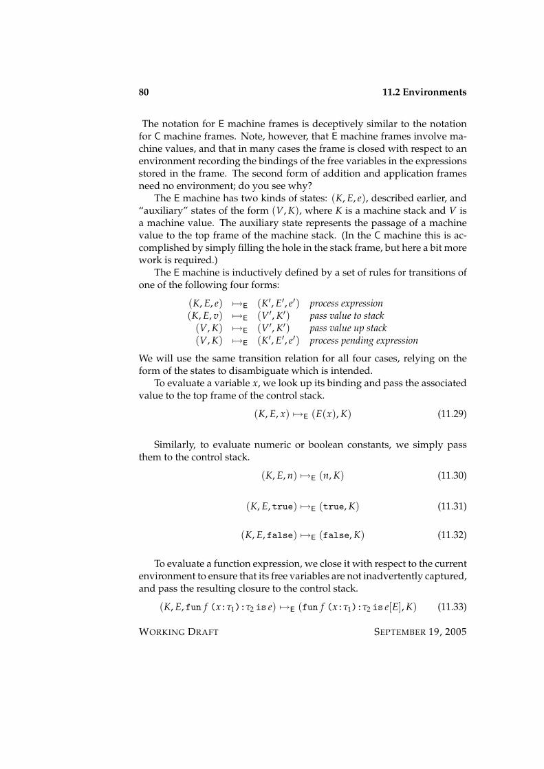
80 11.2 Environments
The notation for E machine frames is deceptively similar to the notationfor C machine frames. Note, however, that E machine frames involve ma-chine values, and that in many cases the frame is closed with respect to anenvironment recording the bindings of the free variables in the expressionsstored in the frame. The second form of addition and application framesneed no environment; do you see why?
The E machine has two kinds of states: (K, E, e), described earlier, and“auxiliary” states of the form (V, K), where K is a machine stack and V isa machine value. The auxiliary state represents the passage of a machinevalue to the top frame of the machine stack. (In the C machine this is ac-complished by simply filling the hole in the stack frame, but here a bit morework is required.)
The E machine is inductively defined by a set of rules for transitions ofone of the following four forms:
(K, E, e) 7→E (K′, E′, e′) process expression(K, E, v) 7→E (V ′, K′) pass value to stack
(V, K) 7→E (V ′, K′) pass value up stack(V, K) 7→E (K′, E′, e′) process pending expression
We will use the same transition relation for all four cases, relying on theform of the states to disambiguate which is intended.
To evaluate a variable x, we look up its binding and pass the associatedvalue to the top frame of the control stack.
(K, E, x) 7→E (E(x), K) (11.29)
Similarly, to evaluate numeric or boolean constants, we simply passthem to the control stack.
(K, E, n) 7→E (n, K) (11.30)
(K, E, true) 7→E (true, K) (11.31)
(K, E, false) 7→E (false, K) (11.32)
To evaluate a function expression, we close it with respect to the currentenvironment to ensure that its free variables are not inadvertently captured,and pass the resulting closure to the control stack.
(K, E, fun f (x:τ1):τ2 is e) 7→E (fun f (x:τ1):τ2 is e[E], K) (11.33)
WORKING DRAFT SEPTEMBER 19, 2005

11.2 Environments 81
To evaluate a primitive operation, we start by evaluating its first argu-ment, pushing a frame on the control stack that records the need to evaluateits remaining arguments.
(K, E, +(e1, e2)) 7→E (+(, e2)[E] . K, E, e1) (11.34)
Notice that the frame is closed in the current environment to avoid captureof free variables in the remaining arguments.
To evaluate a conditional, we evaluate the test expression, pushing aframe on the control stack to record the two pending branches, once againclosed with respect to the current environment.
(K, E, if e then e1 else e2) 7→E (if then e1 else e2[E] . K, E, e) (11.35)
To evaluate an application, we begin by evaluating the function posi-tion, pushing a frame to record the pending evaluation of the argument,closed with respect to the current environment.
(K, E, apply(e1, e2)) 7→E (apply(, e2)[E] . K, E, e1) (11.36)
To complete the definition of the E machine, we must define the transi-tions governing the auxiliary states.
Pending argument evaluations for primitive operations are handled asfollows. If more arguments remain to be evaluated, we switch states toprocess the next argument.
(V1, +(, e2)[E] . K) 7→E (+(V1,) . K, E, e2) (11.37)
Notice that the environment of the frame is used to evaluate the next argu-ment. If no more arguments remain to be evaluated, we pass the result ofexecuting the primitive operation to the rest of the stack.
(n2, +(v1,) . K) 7→E (n1 + n2, K) (11.38)
Pending conditional branches are handled in the obvious manner.
(true, if then e1 else e2[E] . K) 7→E (K, E, e1) (11.39)
(false, if then e1 else e2[E] . K) 7→E (K, E, e2) (11.40)
SEPTEMBER 19, 2005 WORKING DRAFT
82 11.2 Environments
Notice that the environment of the frame is restored before evaluating theappropriate branch of the conditional.
Pending function applications are handled as follows.
(V, apply(, e2)[E] . K) 7→E (apply(V,) . K, E, e2) (11.41)
Observe that the environment of the frame is restored before evaluatingthe argument of the application, and that the function value (which is, pre-sumbly, a closure) is stored intact in the new top frame of the stack.
Once the argument has been evaluated, we call the function.
(V2, apply(V,) . K) 7→E (K, E[ f 7→ V][x 7→ V2], e) (11.42)
whereV = fun f (x:τ1):τ2 is e[E].
To call the function we bind f to V and x to V2 in the environment of the clo-sure, continuing with the evaluation of the body of the function. Observethat since we use the environment of the closure, extended with bindingsfor the function and its parameter, we ensure that the appropriate bindingsfor the free variables of the function are employed.
The final states of the E machine have the form (V, •), with final re-sult V. Notice that the result is a machine value. If the type of the entireprogram is int or bool, then V will be a numeral or a boolean constant,respectively. Otherwise the value will be a closure.
A correspondence between the E and the C machine along the lines ofthe correspondence between the C machine and the M machine may beestablished. However, since the technical details are rather involved, wewill not pursue a rigorous treatment of the relationship here. Suffice it tosay that if e is a closed MinML program of base type (int or bool), then(•, e) 7→∗C (•, v) iff (•, ∅, e) 7→∗E (v, •). (The restriction to base type is neces-sary if we are to claim that both machines return the same value.)
WORKING DRAFT SEPTEMBER 19, 2005
Chapter 12
Continuations
The semantics of many control constructs (such as exceptions and co-routines)can be expressed in terms of reified control stacks, a representation of a con-trol stack as an ordinary value. This is achieved by allowing a stack to bepassed as a value within a program and to be restored at a later point, even ifcontrol has long since returned past the point of reification. Reified controlstacks of this kind are called first-class continuations, where the qualifica-tion “first class” stresses that they are ordinary values with an indefinitelifetime that can be passed and returned at will in a computation. First-class continuations never “expire”, and it is always sensible to reinstate acontinuation without compromising safety. Thus first-class continuationssupport unlimited “time travel” — we can go back to a previous point inthe computation and then return to some point in its future, at will.
How is this achieved? The key to implementing first-class continua-tions is to arrange that control stacks are persistent data structures, just likeany other data structure in ML that does not involve mutable references.By a persistent data structure we mean one for which operations on it yielda “new” version of the data structure without disturbing the old version.For example, lists in ML are persistent in the sense that if we cons an ele-ment to the front of a list we do not thereby destroy the original list, butrather yield a new list with an additional element at the front, retaining thepossibility of using the old list for other purposes. In this sense persistentdata structures allow time travel — we can easily switch between severalversions of a data structure without regard to the temporal order in whichthey were created. This is in sharp contrast to more familiar ephemeral datastructures for which operations such as insertion of an element irrevocablymutate the data structure, preventing any form of time travel.
83
84 12.1 Informal Overview of Continuations
Returning to the case in point, the standard implementation of a controlstack is as an ephemeral data structure, a pointer to a region of mutablestorage that is overwritten whenever we push a frame. This makes it im-possible to maintain an “old” and a “new” copy of the control stack at thesame time, making time travel impossible. If, however, we represent thecontrol stack as a persistent data structure, then we can easily reify a con-trol stack by simply binding it to a variable, and continue working. If wewish we can easily return to that control stack by referring to the variablethat is bound to it. This is achieved in practice by representing the controlstack as a list of frames in the heap so that the persistence of lists can beextended to control stacks. While we will not be specific about implemen-tation strategies in this note, it should be born in mind when consideringthe semantics outlined below.
Why are first-class continuations useful? Fundamentally, they are rep-resentations of the control state of a computation at a given point in time.Using first-class continuations we can “checkpoint” the control state of aprogram, save it in a data structure, and return to it later. In fact this isprecisely what is necessary to implement threads (concurrently executingprograms) — the thread scheduler must be able to checkpoint a programand save it for later execution, perhaps after a pending event occurs or an-other thread yields the processor. In Section 12.3 we will show how to builda threads package for concurrent programming using continuations.
12.1 Informal Overview of Continuations
We will extend MinML with the type τ cont of continuations accepting val-ues of type τ. A continuation will, in fact, be a control stack of type τ stack,but rather than expose this representation to the programmer, we will re-gard τ cont as an abstract type supporting two operations, letcc x in e andthrow e1 to e2.1
Informally, evaluation of letcc x in e binds the current continuation2 tox and evaluates e. The current continuation is, as we’ve discussed, a reifi-cation of the current control stack, which represents the current point in theevaluation of the program. The type of x is τ cont, where τ is the type of e.The intuition is that the current continuation is the point to which e returns
1Close relatives of these primitives are available in SML/NJ in the following forms:for letcc x in e, write SMLofNJ.Cont.callcc (fn x => e), and for throw e1 to e2, writeSMLofNJ.Cont.throw e2 e1.
2Hence the name “letcc”.
WORKING DRAFT SEPTEMBER 19, 2005

12.1 Informal Overview of Continuations 85
when it completes evaluation. Consequently, the control stack expects avalue of type τ, which then determines how execution proceeds. Thus x isbound to a stack expecting a value of type τ, that is, a value of type τ cont.Note that this is the only way to obtain a value of type τ cont; there are noexpressions that evaluate to continuations. (This is similar to our treatmentof references — values of type τ ref are locations, but locations can onlybe obtained by evaluating a ref expression.)
We may “jump” to a saved control point by throwing a value to a contin-uation, written throw e1 to e2. The expression e2 must evaluate to a τ1 cont,and e1 must evaluate to a value of type τ1. The current control stack is aban-doned in favor of the reified control stack resulting from the evaluation ofe2; the value of e1 is then passed to that stack.
Here is a simple example, written in Standard ML notation. The idea isto multiply the elements of a list, short-circuiting the computation in case 0is encountered. Here’s the code:
fun mult list (l:int list):int =letcc ret inlet fun mult nil = 1
| mult (0:: ) = throw 0 to ret| mult (n::l) = n * mult l
in mult l end )
Ignoring the letcc for the moment, the body of mult list is a let expres-sion that defines a recursive procedure mult, and applies it to the argumentof mult list. The job of mult is to return the product of the elements of thelist. Ignoring the second line of mult, it should be clear why and how thiscode works.
Now let’s consider the second line of mult, and the outer use of letcc.Intuitively, the purpose of the second line of mult is to short circuit the mul-tiplication, returning 0 immediately in the case that a 0 occurs in the list.This is achieved by throwing the value 0 (the final answer) to the continua-tion bound to the variable ret. This variable is bound by letcc surround-ing the body of mult list. What continuation is it? It’s the continuationthat runs upon completion of the body of mult list. This continuationwould be executed in the case that no 0 is encountered and evaluation pro-ceeds normally. In the unusual case of encountering a 0 in the list, webranch directly to the return point, passing the value 0, effecting an earlyreturn from the procedure with result value 0.
Here’s another formulation of the same function:
SEPTEMBER 19, 2005 WORKING DRAFT
86 12.1 Informal Overview of Continuations
fun mult list l =let fun mult nil ret = 1
| mult (0:: ) ret = throw 0 to ret| mult (n::l) ret = n * mult l ret
in letcc ret in (mult l) ret end
Here the inner loop is parameterized by the return continuation for earlyexit. The multiplication loop is obtained by calling mult with the currentcontinuation at the exit point of mult list so that throws to ret effect anearly return from mult list, as desired.
Let’s look at another example: given a continuation k of type τ cont anda function f of type τ′→τ, return a continuation k′ of type τ′ cont with thefollowing behavior: throwing a value v′ of type τ′ to k′ throws the valuef (v′) to k. This is called composition of a function with a continuation. Wewish to fill in the following template:
fun compose (f:τ′->τ,k:τ cont):τ′ cont = ...
The function compose will have type
((τ′ -> τ) * τ cont) -> τ′ cont
The first problem is to obtain the continuation we wish to return. Thesecond problem is how to return it. The continuation we seek is the one ineffect at the point of the ellipsis in the expression throw f(...) to k. Thisis the continuation that, when given a value v′, applies f to it, and throwsthe result to k. We can seize this continuation using letcc, writing
throw f(letcc x:τ′ cont in ...) to k
At the point of the ellipsis the variable x is bound to the continuation wewish to return. How can we return it? By using the same trick as we usedfor short-circuiting evaluation above! We don’t want to actually throw avalue to this continuation (yet), instead we wish to abort it and return it asthe result. Here’s the final code:
fun compose (f, k) =letcc ret inthrow (f (letcc r in throw r to ret)) to k
The type of ret is τ′ cont cont, a continuation expecting a continuationexpecting a value of type τ′!
WORKING DRAFT SEPTEMBER 19, 2005

12.2 Semantics of Continuations 87
We can do without first-class continuations by “rolling our own”. Theidea is that we can perform (by hand or automatically) a systematic pro-gram transformation in which a “copy” of the control stack is maintainedas a function, called a continuation. Every function takes as an argumentthe control stack to which it is to pass its result by applying given stack(represented as a function) to the result value. Functions never return inthe usual sense; they pass their result to the given continuation. Programswritten in this form are said to be in continuation-passing style, or CPS forshort.
Here’s the code to multiply the elements of a list (without short-circuiting)in continuation-passing style:
fun cps mult nil k = k 1| cps mult (n::l) k = cps mult l (fn r => k (n * r))
fun mult l = cps mult l (fn r => r)
It’s easy to implement the short-circuit form by passing an additionalcontinuation, the one to invoke for short-circuiting the result:
fun cps mult list l k =let fun cps mult nil k0 k = k 1| fun cps mult (0:: ) k0 k = k0 0| fun cps mult (n::l) k0 k = cps mult k0 l (fn p => k (n*p))
in cps mult l k k end
The continuation k0 never changes; it is always the return continuation forcps mult list. The argument continuation to cps mult list is duplicatedon the call to cps mult.
Observe that the type of the first version of cps mult becomes
int list→(int→α)→α,
and that the type of the second version becomes
int list→(int→α)→(int→α)→α,
These transformations are representative of the general case.
12.2 Semantics of Continuations
The informal description of evaluation is quite complex, as you no doubthave observed. Here’s an example where a formal semantics is much clearer,
SEPTEMBER 19, 2005 WORKING DRAFT
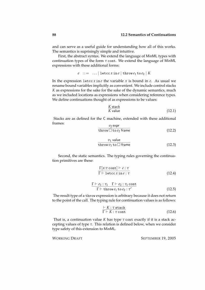
88 12.2 Semantics of Continuations
and can serve as a useful guide for understanding how all of this works.The semantics is suprisingly simple and intuitive.
First, the abstract syntax. We extend the language of MinML types withcontinuation types of the form τ cont. We extend the language of MinMLexpressions with these additional forms:
e : : = . . . | letcc x in e | throw e1 to e2 | K
In the expression letcc x in e the variable x is bound in e. As usual werename bound variables implicitly as convenient. We include control stacksK as expressions for the sake for the sake of the dynamic semantics, muchas we included locations as expressions when considering reference types.We define continuations thought of as expressions to be values:
K stackK value (12.1)
Stacks are as defined for the C machine, extended with these additionalframes: e2 expr
throw to e2 frame (12.2)
v1 value
throw v1 to frame (12.3)
Second, the static semantics. The typing rules governing the continua-tion primitives are these:
Γ[x:τ cont] ` e : τ
Γ ` letcc x in e : τ (12.4)
Γ ` e1 : τ1 Γ ` e2 : τ1 cont
Γ ` throw e1 to e2 : τ′ (12.5)
The result type of a throw expression is arbitrary because it does not returnto the point of the call. The typing rule for continuation values is as follows:
` K : τ stackΓ ` K : τ cont (12.6)
That is, a continuation value K has type τ cont exactly if it is a stack ac-cepting values of type τ. This relation is defined below, when we considertype safety of this extension to MinML.
WORKING DRAFT SEPTEMBER 19, 2005
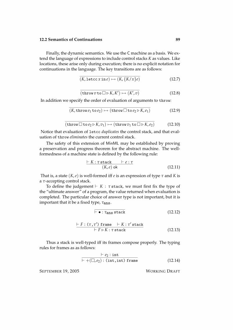
12.2 Semantics of Continuations 89
Finally, the dynamic semantics. We use the C machine as a basis. We ex-tend the language of expressions to include control stacks K as values. Likelocations, these arise only during execution; there is no explicit notation forcontinuations in the language. The key transitions are as follows:
(K, letcc x in e) 7→ (K, K/xe) (12.7)
(throw v to . K, K′) 7→ (K′, v) (12.8)
In addition we specify the order of evaluation of arguments to throw:
(K, throw e1 to e2) 7→ (throw to e2 . K, e1) (12.9)
(throw to e2 . K, v1) 7→ (throw v1 to . K, e2) (12.10)
Notice that evaluation of letcc duplicates the control stack, and that eval-uation of throw eliminates the current control stack.
The safety of this extension of MinML may be established by provinga preservation and progress theorem for the abstract machine. The well-formedness of a machine state is defined by the following rule:
` K : τ stack ` e : τ(K, e) ok (12.11)
That is, a state (K, e) is well-formed iff e is an expression of type τ and K isa τ-accepting control stack.
To define the judgement ` K : τ stack, we must first fix the type ofthe “ultimate answer” of a program, the value returned when evaluation iscompleted. The particular choice of answer type is not important, but it isimportant that it be a fixed type, τans.
` • : τans stack (12.12)
` F : (τ,τ′) frame ` K : τ′ stack` F . K : τ stack (12.13)
Thus a stack is well-typed iff its frames compose properly. The typingrules for frames as as follows:
` e2 : int` +(, e2) : (int,int) frame (12.14)
SEPTEMBER 19, 2005 WORKING DRAFT
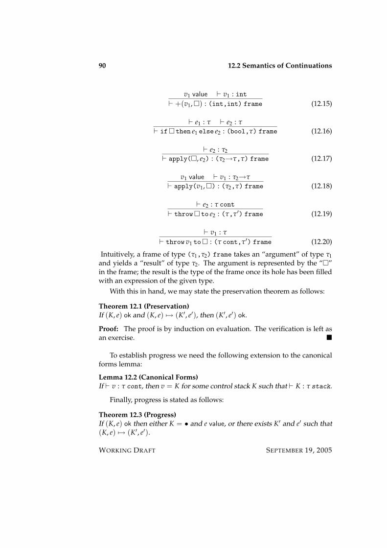
90 12.2 Semantics of Continuations
v1 value ` v1 : int` +(v1,) : (int,int) frame (12.15)
` e1 : τ ` e2 : τ
` if then e1 else e2 : (bool,τ) frame (12.16)
` e2 : τ2
` apply(, e2) : (τ2→τ,τ) frame (12.17)
v1 value ` v1 : τ2→τ
` apply(v1,) : (τ2,τ) frame (12.18)
` e2 : τ cont
` throw to e2 : (τ,τ′) frame (12.19)
` v1 : τ
` throw v1 to : (τ cont,τ′) frame (12.20)
Intuitively, a frame of type (τ1,τ2) frame takes an “argument” of type τ1and yields a “result” of type τ2. The argument is represented by the “”in the frame; the result is the type of the frame once its hole has been filledwith an expression of the given type.
With this in hand, we may state the preservation theorem as follows:
Theorem 12.1 (Preservation)If (K, e) ok and (K, e) 7→ (K′, e′), then (K′, e′) ok.
Proof: The proof is by induction on evaluation. The verification is left asan exercise.
To establish progress we need the following extension to the canonicalforms lemma:
Lemma 12.2 (Canonical Forms)If ` v : τ cont, then v = K for some control stack K such that ` K : τ stack.
Finally, progress is stated as follows:
Theorem 12.3 (Progress)If (K, e) ok then either K = • and e value, or there exists K′ and e′ such that(K, e) 7→ (K′, e′).
WORKING DRAFT SEPTEMBER 19, 2005
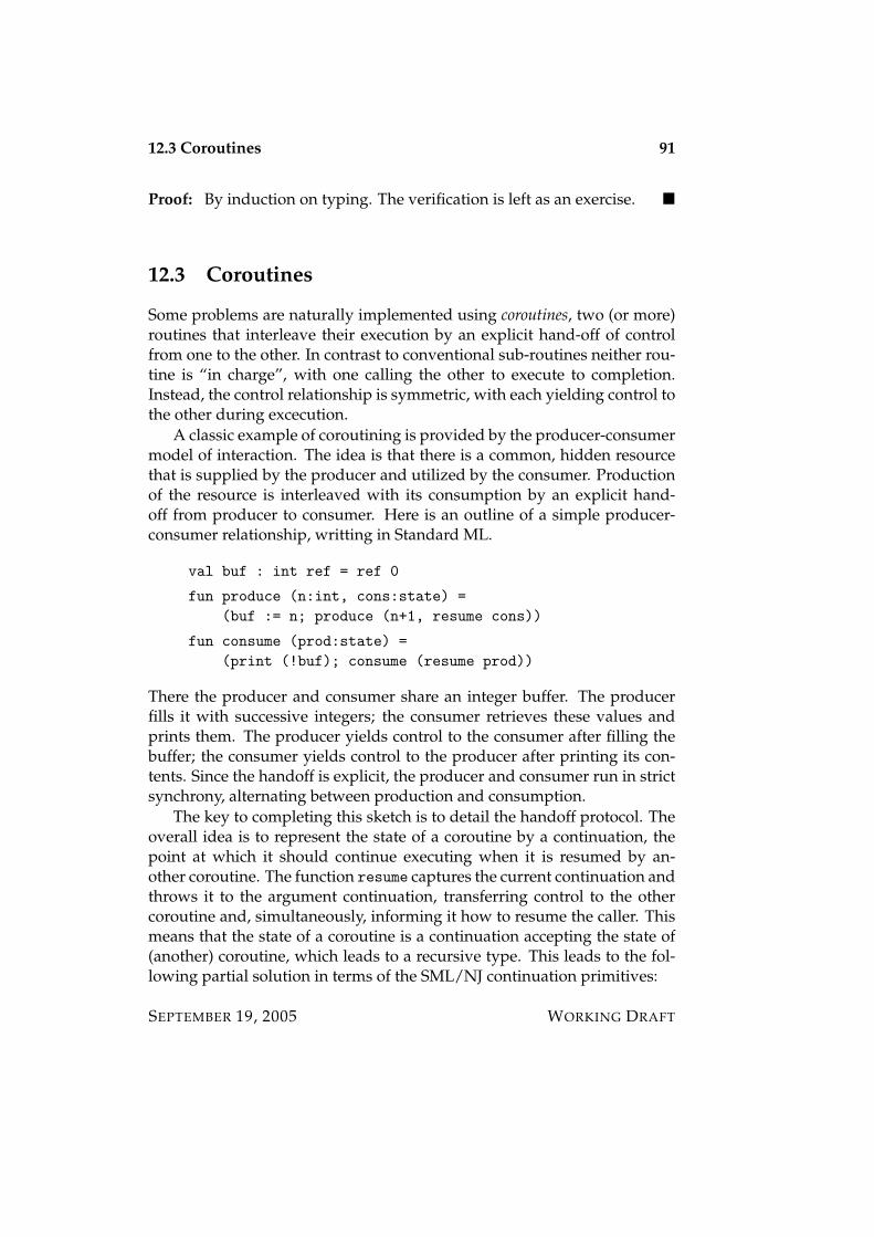
12.3 Coroutines 91
Proof: By induction on typing. The verification is left as an exercise.
12.3 Coroutines
Some problems are naturally implemented using coroutines, two (or more)routines that interleave their execution by an explicit hand-off of controlfrom one to the other. In contrast to conventional sub-routines neither rou-tine is “in charge”, with one calling the other to execute to completion.Instead, the control relationship is symmetric, with each yielding control tothe other during excecution.
A classic example of coroutining is provided by the producer-consumermodel of interaction. The idea is that there is a common, hidden resourcethat is supplied by the producer and utilized by the consumer. Productionof the resource is interleaved with its consumption by an explicit hand-off from producer to consumer. Here is an outline of a simple producer-consumer relationship, writting in Standard ML.
val buf : int ref = ref 0
fun produce (n:int, cons:state) =(buf := n; produce (n+1, resume cons))
fun consume (prod:state) =(print (!buf); consume (resume prod))
There the producer and consumer share an integer buffer. The producerfills it with successive integers; the consumer retrieves these values andprints them. The producer yields control to the consumer after filling thebuffer; the consumer yields control to the producer after printing its con-tents. Since the handoff is explicit, the producer and consumer run in strictsynchrony, alternating between production and consumption.
The key to completing this sketch is to detail the handoff protocol. Theoverall idea is to represent the state of a coroutine by a continuation, thepoint at which it should continue executing when it is resumed by an-other coroutine. The function resume captures the current continuation andthrows it to the argument continuation, transferring control to the othercoroutine and, simultaneously, informing it how to resume the caller. Thismeans that the state of a coroutine is a continuation accepting the state of(another) coroutine, which leads to a recursive type. This leads to the fol-lowing partial solution in terms of the SML/NJ continuation primitives:
SEPTEMBER 19, 2005 WORKING DRAFT
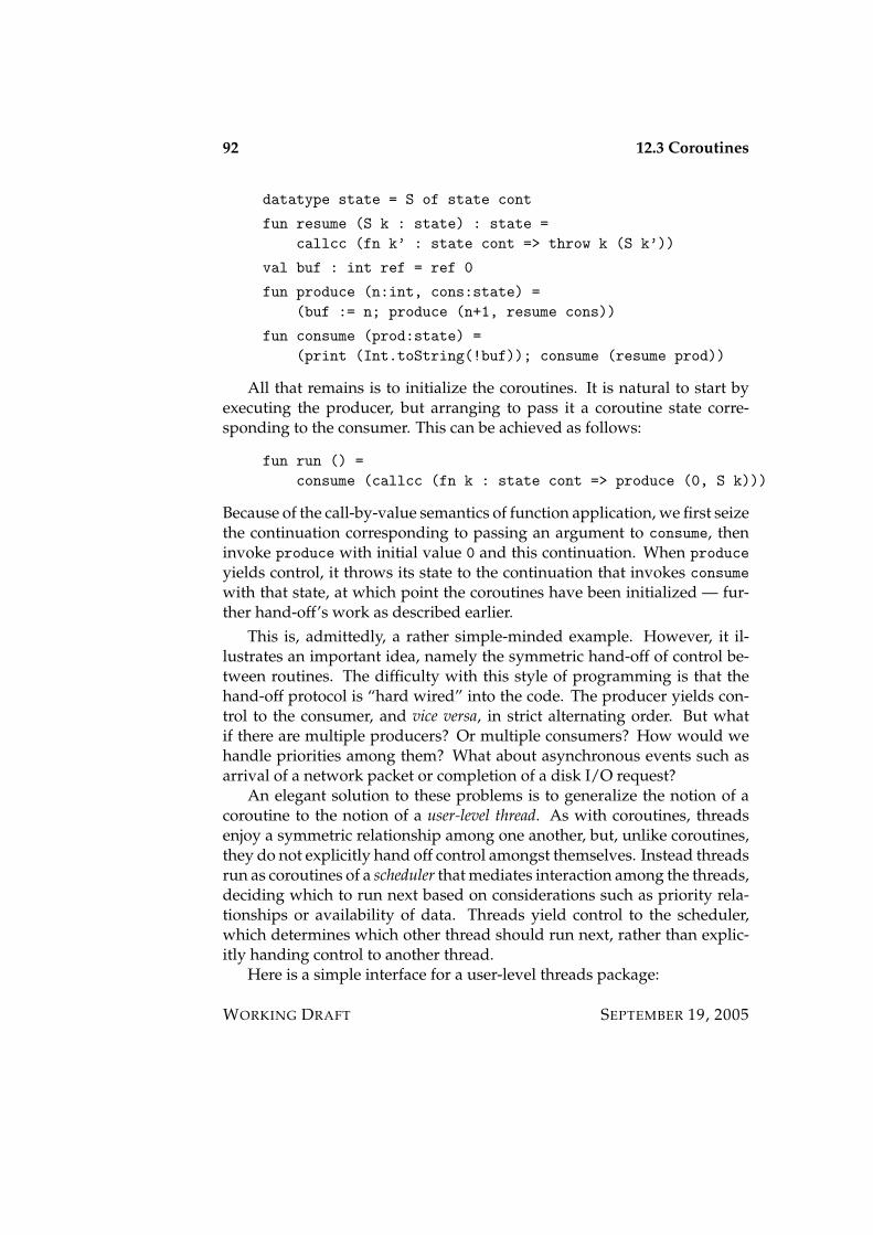
92 12.3 Coroutines
datatype state = S of state cont
fun resume (S k : state) : state =callcc (fn k’ : state cont => throw k (S k’))
val buf : int ref = ref 0
fun produce (n:int, cons:state) =(buf := n; produce (n+1, resume cons))
fun consume (prod:state) =(print (Int.toString(!buf)); consume (resume prod))
All that remains is to initialize the coroutines. It is natural to start byexecuting the producer, but arranging to pass it a coroutine state corre-sponding to the consumer. This can be achieved as follows:
fun run () =consume (callcc (fn k : state cont => produce (0, S k)))
Because of the call-by-value semantics of function application, we first seizethe continuation corresponding to passing an argument to consume, theninvoke produce with initial value 0 and this continuation. When produceyields control, it throws its state to the continuation that invokes consumewith that state, at which point the coroutines have been initialized — fur-ther hand-off’s work as described earlier.
This is, admittedly, a rather simple-minded example. However, it il-lustrates an important idea, namely the symmetric hand-off of control be-tween routines. The difficulty with this style of programming is that thehand-off protocol is “hard wired” into the code. The producer yields con-trol to the consumer, and vice versa, in strict alternating order. But whatif there are multiple producers? Or multiple consumers? How would wehandle priorities among them? What about asynchronous events such asarrival of a network packet or completion of a disk I/O request?
An elegant solution to these problems is to generalize the notion of acoroutine to the notion of a user-level thread. As with coroutines, threadsenjoy a symmetric relationship among one another, but, unlike coroutines,they do not explicitly hand off control amongst themselves. Instead threadsrun as coroutines of a scheduler that mediates interaction among the threads,deciding which to run next based on considerations such as priority rela-tionships or availability of data. Threads yield control to the scheduler,which determines which other thread should run next, rather than explic-itly handing control to another thread.
Here is a simple interface for a user-level threads package:
WORKING DRAFT SEPTEMBER 19, 2005
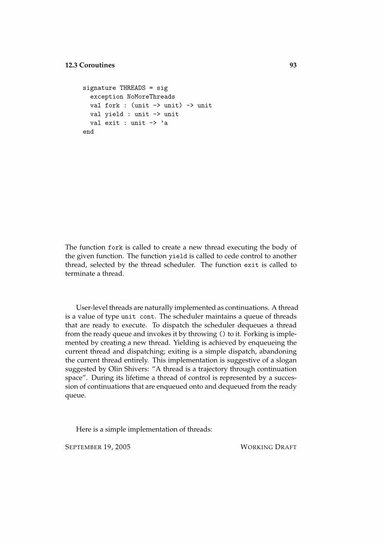
12.3 Coroutines 93
signature THREADS = sigexception NoMoreThreadsval fork : (unit -> unit) -> unitval yield : unit -> unitval exit : unit -> ’a
end
The function fork is called to create a new thread executing the body ofthe given function. The function yield is called to cede control to anotherthread, selected by the thread scheduler. The function exit is called toterminate a thread.
User-level threads are naturally implemented as continuations. A threadis a value of type unit cont. The scheduler maintains a queue of threadsthat are ready to execute. To dispatch the scheduler dequeues a threadfrom the ready queue and invokes it by throwing () to it. Forking is imple-mented by creating a new thread. Yielding is achieved by enqueueing thecurrent thread and dispatching; exiting is a simple dispatch, abandoningthe current thread entirely. This implementation is suggestive of a slogansuggested by Olin Shivers: “A thread is a trajectory through continuationspace”. During its lifetime a thread of control is represented by a succes-sion of continuations that are enqueued onto and dequeued from the readyqueue.
Here is a simple implementation of threads:
SEPTEMBER 19, 2005 WORKING DRAFT

94 12.3 Coroutines
structure Threads :> THREADS = structopen SMLofNJ.Contexception NoRunnableThreadstype thread = unit contval readyQueue : thread Queue.queue = Queue.mkQueue()fun dispatch () =
letval t = Queue.dequeue readyQueue
handle Queue.Dequeue => raise NoRunnableThreadsin
throw t ()end
fun exit () = dispatch()fun enqueue t = Queue.enqueue (readyQueue, t)fun fork f =
callcc (fn parent => (enqueue parent; f (); exit()))fun yield () =
callcc (fn parent => (enqueue parent; dispatch()))end
Using the above thread interface we may implement the simple producer-consumer example as follows:
structure Client = structopen Threadsval buffer : int ref = ref (~1)fun producer (n) =
(buffer := n ; yield () ; producer (n+1))fun consumer () =
(print (Int.toString (!buffer)); yield (); consumer())fun run () =
(fork (consumer); producer 0)end
This example is excessively naıve, however, in that it relies on the strictFIFO ordering of threads by the scheduler, allowing careful control overthe order of execution. If, for example, the producer were to run severaltimes in a row before the consumer could run, several numbers would beomitted from the output.
Here is a better solution that avoids this problem (but does so by “busywaiting”):
WORKING DRAFT SEPTEMBER 19, 2005

12.4 Exercises 95
structure Client = structopen Threadsval buffer : int option ref = ref NONEfun producer (n) =
(case !bufferof NONE => (buffer := SOME n ; yield() ; producer (n+1))| SOME => (yield (); producer (n)))
fun consumer () =(case !buffer
of NONE => (yield (); consumer())| SOME n =>(print (Int.toString n); buffer := NONE; yield(); consumer()))
fun run () =(fork (consumer); producer 0)
end
There is much more to be said about threads! We will return to thislater in the course. For now, the main idea is to give a flavor of how first-class continuations can be used to implement a user-level threads packagewith very little difficulty. A more complete implementation is, of course,somewhat more complex, but not much more. We can easily provide allthat is necessary for sophisticated thread programming in a few hundredlines of ML code.
12.4 Exercises
1. Study the short-circuit multiplication example carefully to be sureyou understand why it works!
2. Attempt to solve the problem of composing a continuation with afunction yourself, before reading the solution.
3. Simulate the evaluation of compose ( f, k) on the empty stack. Ob-serve that the control stack substituted for x is
apply( f ,) . throw to k . • (12.21)
This stack is returned from compose. Next, simulate the behavior ofthrowing a value v′ to this continuation. Observe that the above stackis reinstated and that v′ is passed to it.
SEPTEMBER 19, 2005 WORKING DRAFT

96 12.4 Exercises
WORKING DRAFT SEPTEMBER 19, 2005

Chapter 13
Exceptions
Exceptions effects a non-local transfer of control from the point at whichthe exception is raised to a dynamically enclosing handler for that excep-tion. This transfer interrupts the normal flow of control in a program inresponse to unusual conditions. For example, exceptions can be used tosignal an error condition, or to indicate the need for special handling incertain circumstances that arise only rarely. To be sure, one could use ex-plicit conditionals to check for and process errors or unusual conditions,but using exceptions is often more convenient, particularly since the trans-fer to the handler is direct and immediate, rather than indirect via a seriesof explicit checks. All too often explicit checks are omitted (by design orneglect), whereas exceptions cannot be ignored.
We’ll consider the extension of MinML with an exception mechanismsimilar to that of Standard ML, with the significant simplification that novalue is associated with the exception — we simply signal the exceptionand thereby invoke the nearest dynamically enclosing handler. We’ll comeback to consider value-passing exceptions later.
The following grammar describes the extensions to MinML to supportvalueless exceptions:
e : : = . . . | fail | try e1 ow e2
The expression fail raises an exception. The expression try e1 ow e2 evalu-ates e1. If it terminates normally, we return its value; otherwise, if it fails,we continue by evaluating e2.
The static semantics of exceptions is quite straightforward:
Γ ` fail : τ (13.1)
97
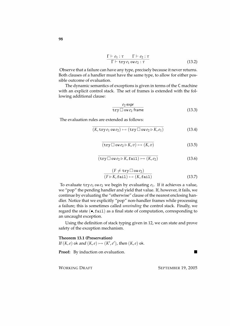
98
Γ ` e1 : τ Γ ` e2 : τ
Γ ` try e1 ow e2 : τ (13.2)
Observe that a failure can have any type, precisely because it never returns.Both clauses of a handler must have the same type, to allow for either pos-sible outcome of evaluation.
The dynamic semantics of exceptions is given in terms of the C machinewith an explicit control stack. The set of frames is extended with the fol-lowing additional clause:
e2 expr
try ow e2 frame (13.3)
The evaluation rules are extended as follows:
(K, try e1 ow e2) 7→ (try ow e2 . K, e1) (13.4)
(try ow e2 . K, v) 7→ (K, v) (13.5)
(try ow e2 . K, fail) 7→ (K, e2) (13.6)
(F 6= try ow e2)(F . K, fail) 7→ (K, fail) (13.7)
To evaluate try e1 ow e2 we begin by evaluating e1. If it achieves a value,we “pop” the pending handler and yield that value. If, however, it fails, wecontinue by evaluating the “otherwise” clause of the nearest enclosing han-dler. Notice that we explicitly “pop” non-handler frames while processinga failure; this is sometimes called unwinding the control stack. Finally, weregard the state (•, fail) as a final state of computation, corresponding toan uncaught exception.
Using the definition of stack typing given in 12, we can state and provesafety of the exception mechanism.
Theorem 13.1 (Preservation)If (K, e) ok and (K, e) 7→ (K′, e′), then (K, e) ok.
Proof: By induction on evaluation.
WORKING DRAFT SEPTEMBER 19, 2005

99
Theorem 13.2 (Progress)If (K, e) ok then either
1. K = • and e value, or
2. K = • and e = fail, or
3. there exists K′ and e′ such that (K, e) 7→ (K′, e′).
Proof: By induction on typing.
The dynamic semantics of exceptions is somewhat unsatisfactory be-cause of the explicit unwinding of the control stack to find the nearest en-closing handler. While this does effect a non-local transfer of control, it doesso by rather crude means, rather than by a direct “jump” to the handler. Inpractice exceptions are implemented as jumps, using the following ideas.A dedicated register is set aside to contain the “current” exception handler.When an exception is raised, the current handler is retrieved from the ex-ception register, and control is passed to it. Before doing so, however, wemust reset the exception register to contain the nearest handler enclosingthe new handler. This ensures that if the handler raises an exception thecorrect handler is invoked. How do we recover this handler? We maintaina stack of pending handlers that is pushed whenever a handler is installed,and popped whenever a handler is invoked. The exception register is thetop element of this stack. Note that we must restore the control stack to thepoint at which the handler was installed before invoking the handler!
This can be modelled by a machine with states of the form (H, K, e),where
• H is a handler stack;
• K is a control stack;
• e is a closed expression
A handler stack consists of a stack of pairs consisting of a handler togetherits associated control stack:
• hstack (13.8)
K stack e expr H hstack
(K, e) . H hstack (13.9)
A handler stack element consists of a “freeze dried” control stack pairedwith a pending handler.
SEPTEMBER 19, 2005 WORKING DRAFT
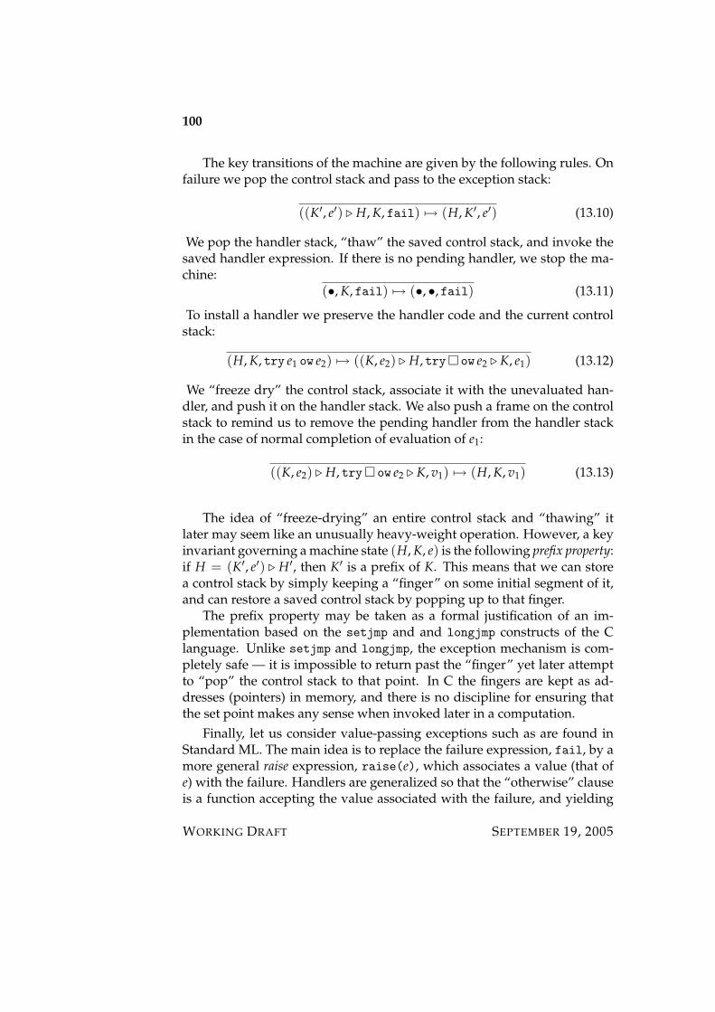
100
The key transitions of the machine are given by the following rules. Onfailure we pop the control stack and pass to the exception stack:
((K′, e′) . H, K, fail) 7→ (H, K′, e′) (13.10)
We pop the handler stack, “thaw” the saved control stack, and invoke thesaved handler expression. If there is no pending handler, we stop the ma-chine:
(•, K, fail) 7→ (•, •, fail) (13.11)
To install a handler we preserve the handler code and the current controlstack:
(H, K, try e1 ow e2) 7→ ((K, e2) . H, try ow e2 . K, e1) (13.12)
We “freeze dry” the control stack, associate it with the unevaluated han-dler, and push it on the handler stack. We also push a frame on the controlstack to remind us to remove the pending handler from the handler stackin the case of normal completion of evaluation of e1:
((K, e2) . H, try ow e2 . K, v1) 7→ (H, K, v1) (13.13)
The idea of “freeze-drying” an entire control stack and “thawing” itlater may seem like an unusually heavy-weight operation. However, a keyinvariant governing a machine state (H, K, e) is the following prefix property:if H = (K′, e′) . H′, then K′ is a prefix of K. This means that we can storea control stack by simply keeping a “finger” on some initial segment of it,and can restore a saved control stack by popping up to that finger.
The prefix property may be taken as a formal justification of an im-plementation based on the setjmp and and longjmp constructs of the Clanguage. Unlike setjmp and longjmp, the exception mechanism is com-pletely safe — it is impossible to return past the “finger” yet later attemptto “pop” the control stack to that point. In C the fingers are kept as ad-dresses (pointers) in memory, and there is no discipline for ensuring thatthe set point makes any sense when invoked later in a computation.
Finally, let us consider value-passing exceptions such as are found inStandard ML. The main idea is to replace the failure expression, fail, by amore general raise expression, raise(e), which associates a value (that ofe) with the failure. Handlers are generalized so that the “otherwise” clauseis a function accepting the value associated with the failure, and yielding
WORKING DRAFT SEPTEMBER 19, 2005
101
a value of the same type as the “try” clause. Here is a sketch of the staticsemantics for this variation:
Γ ` e : τexn
Γ ` raise(e) : τ (13.14)
Γ ` e1 : τ Γ ` e2 : τexn→τ
Γ ` try e1 ow e2 : τ (13.15)
These rules are parameterized by the type of values associated with excep-tions, τexn.
The question is: what should be the type τexn? The first thing to observeis that all exceptions should be of the same type, otherwise we cannot guar-antee type safety. The reason is that a handler might be invoked by anyraise expression occurring during the execution of its “try” clause. If oneexception raised an integer, and another a boolean, the handler could notsafely dispatch on the exception value. Given this, we must choose a typeτexn that supports a flexible programming style.
For example, we might choose, say, string, for τexn, with the idea thatthe value associated with an exception is a description of the cause of theexception. For example, we might write
fun div (m, 0) = raise "Division by zero attempted."| div (m, n) = ... raise "Arithmetic overflow occurred." ...
However, consider the plight of the poor handler, which may wish to dis-tinguish between division-by-zero and arithmetic overflow. How might itdo that? If exception values were strings, it would have to parse the string,relying on the message to be in a standard format, and dispatch based onthe parse. This is manifestly unworkable. For similar reasons we wouldn’tchoose τexn to be, say, int, since that would require coding up exceptions asnumbers, much like “error numbers” in Unix. Again, completely unwork-able in practice, and completely unmodular (different modules are boundto conflict over their numbering scheme).
A more reasonable choice would be to define τexn to be a given datatypeexc. For example, we might have the declaration
datatype exc = Div | Overflow | Match | Bind
as part of the implicit prelude of every program. Then we’d write
fun div (m, 0) = raise Div| div (m, n) = ... raise Overflow ...
SEPTEMBER 19, 2005 WORKING DRAFT
102 13.1 Exercises
Now the handler can easily dispatch on Div or Overflow using patternmatching, which is much better. However, this choice restricts all programsto a fixed set of exceptions, the value constructors associated with the pre-declared exc datatype.
To allow extensibility Standard ML includes a special extensible datatypecalled exn. Values of type exn are similar to values of a datatype, namelythey are constructed from other values using a constructor. Moreover, wemay pattern match against values of type exn in the usual way. But, in ad-dition, we may introduce new constructors of type exn “on the fly”, ratherthan declare a fixed set at the beginning of the program. Such new con-structors are introduced using an exception declaration such as the follow-ing:
exception Divexception Overflow
Now Div and Overflow are constructors of type exn, and may be used ina raise expression or matched against by an exception handler. Exceptiondeclarations can occur anywhere in the program, and are guaranteed (byα-conversion) to be distinct from all other exceptions that may occur else-where in the program, even if they happen to have the same name. If twomodules declare an exception named Error, then these are different excep-tions; no confusion is possible.
The interesting thing about the exn type is that it has nothing whatsoeverto do with the exception mechanism (beyond the fact that it is the type of val-ues associated with exceptions). In particular, the exception declarationintroduces a value constructor that has no inherent connection with the ex-ception mechanism. We may use the exn type for other purposes; indeed,Java has an analogue of the type exn, called Object. This is the basis fordowncasting and so-called typecase in Java.
13.1 Exercises
1. Hand-simulate the evaluation of a few simple expressions with ex-ceptions and handlers to get a feeling for how it works.
2. Prove Theorem 13.1.
3. Prove Theorem 13.2.
WORKING DRAFT SEPTEMBER 19, 2005
13.1 Exercises 103
4. Combine the treatment of references and exceptions to form a lan-guage with both of these features. You will face a choice of how todefine the interaction between mutation and exceptions:
(a) As in ML, mutations are irrevocable, even in the face of excep-tions that “backtrack” to a surrounding handler.
(b) Invocation of a handler rolls back the memory to the state at thepoint of installation of the handler.
Give a dynamic semantics for each alternative, and argue for andagainst each choice.
5. State and prove the safety of the formulation of exceptions using ahandler stack.
6. Prove that the prefix property is preserved by every step of evalua-tion.
SEPTEMBER 19, 2005 WORKING DRAFT

104 13.1 Exercises
WORKING DRAFT SEPTEMBER 19, 2005
Part V
Imperative FunctionalProgramming
105

Chapter 14
Mutable Storage
MinML is said to be a pure language because the execution model consistsentirely of evaluating an expression for its value. ML is an impure languagebecause its execution model also includes effects, specifically, control effectsand store effects. Control effects are non-local transfers of control; these werestudied in Chapters 12 and 13. Store effects are dynamic modifications tomutable storage. This chapter is concerned with store effects.
14.1 References
The MinML type language is extended with reference types τ ref whose el-ements are to be thought of as mutable storage cells. We correspondinglyextend the expression language with these primitive operations:
e : : = l | ref(e) | !e | e1:=e2
As in Standard ML, ref(e) allocates a “new” reference cell, !e retrieves thecontents of the cell e, and e1:=e2 sets the contents of the cell e1 to the valuee2. The variable l ranges over a set of locations, an infinite set of identifiersdisjoint from variables. These are needed for the dynamic semantics, butare not expected to be notated directly by the programmer. The set of valuesis extended to include locations.
Typing judgments have the form Λ; Γ ` e : τ, where Λ is a location typ-ing, a finite function mapping locations to types; the other components ofthe judgement are as for MinML. The location typing Λ records the types ofallocated locations during execution; this is critical for a precise statementand proof of type soundness.
107
108 14.1 References
The typing rules are those of MinML (extended to carry a location typ-ing), plus the following rules governing the new constructs of the language:
(Λ(l) = τ)Λ; Γ ` l : τ ref (14.1)
Λ; Γ ` e : τ
Λ; Γ ` ref(e) : τ ref (14.2)
Λ; Γ ` e : τ refΛ; Γ ` !e : τ (14.3)
Λ; Γ ` e1 : τ2 ref Λ; Γ ` e2 : τ2
Λ; Γ ` e1:=e2 : τ2 (14.4)
Notice that the location typing is not extended during type checking! Loca-tions arise only during execution, and are not part of complete programs,which must not have any free locations in them. The role of the locationtyping will become apparent in the proof of type safety for MinML extendedwith references.
A memory is a finite function mapping locations to closed values (butpossibly involving locations). The dynamic semantics of MinML with refer-ences is given by an abstract machine. The states of this machine have theform (M, e), where M is a memory and e is an expression possibly involv-ing free locations in the domain of M. The locations in dom(M) are boundsimultaneously in (M, e); the names of locations may be changed at willwithout changing the identity of the state.
The transitions for this machine are similar to those of the M machine,but with these additional steps:
(M, e) 7→ (M′, e′)(M, ref(e)) 7→ (M′, ref(e′)) (14.5)
(l /∈ dom(M))(M, ref(v)) 7→ (M[l=v], l) (14.6)
(M, e) 7→ (M′, e′)(M, !e) 7→ (M′, !e′) (14.7)
WORKING DRAFT SEPTEMBER 19, 2005

14.1 References 109
(l ∈ dom(M))(M, !l) 7→ (M, M(l)) (14.8)
(M, e1) 7→ (M′, e′1)(M, e1:=e2) 7→ (M′, e′1:=e2) (14.9)
(M, e2) 7→ (M′, e′2)(M, v1:=e2) 7→ (M′, v1:=e′2) (14.10)
(l ∈ dom(M))(M, l:=v) 7→ (M[l=v], v) (14.11)
A state (M, e) is final iff e is a value (possibly a location).To prove type safety for this extension we will make use of some auxil-
iary relations. Most importantly, the typing relation between memories andlocation typings, written ` M : Λ, is inductively defined by the followingrule:
dom(M) = dom(Λ) ∀l ∈ dom(Λ) Λ; • ` M(l) : Λ(l)` M : Λ (14.12)
It is very important to study this rule carefully! First, we require that Λand M govern the same set of locations. Second, for each location l in theircommon domain, we require that the value at location l, namely M(l), havethe type assigned to l, namely Λ(l), relative to the entire location typing Λ.This means, in particular, that memories may be “circular” in the sense thatthe value at location l may contain an occurrence of l, for example if thatvalue is a function.
The typing rule for memories is reminiscent of the typing rule for recur-sive functions — we are allowed to assume the typing that we are tryingto prove while trying to prove it. This similarity is no accident, as the fol-lowing example shows. Here we use ML notation, but the example can bereadily translated into MinML extended with references:
SEPTEMBER 19, 2005 WORKING DRAFT
110 14.1 References
(* loop forever when called *)fun diverge (x:int):int = diverge x(* allocate a reference cell *)val fc : (int->int) ref = ref (diverge)(* define a function that ‘‘recurs’’ through fc *)fun f 0 = 1 | f n = n * ((!fc)(n-1))(* tie the knot *)val = fc := f(* now call f *)val n = f 5
This technique is called backpatching. It is used in some compilers to imple-ment recursive functions (and other forms of looping construct).
Exercise 14.11. Sketch the contents of the memory after each step in the above exam-
ple. Observe that after the assignment to fc the memory is “circular”in the sense that some location contains a reference to itself.
2. Prove that every cycle in well-formed memory must “pass through”a function. Suppose that M(l1) = l2, M(l2) = l3, . . . , M(ln) = l1 forsome sequence l1, . . . , ln of locations. Show that there is no locationtyping Λ such that ` M : Λ.
The well-formedness of a machine state is inductively defined by thefollowing rule:
` M : Λ Λ; • ` e : τ
(M, e) ok (14.13)
That is, (M, e) is well-formed iff there is a location typing for M relative towhich e is well-typed.
Theorem 14.2 (Preservation)If (M, e) ok and (M, e) 7→ (M′, e′), then (M′, e′) ok.
Proof: The trick is to prove a stronger result by induction on evaluation: if(M, e) 7→ (M′, e′), ` M : Λ, and Λ; • ` e : τ, then there exists Λ′ ⊇ Λ suchthat ` M′ : Λ′ and Λ′; • ` e′ : τ.
Exercise 14.3Prove Theorem 14.2. The strengthened form tells us that the location typ-ing, and the memory, increase monotonically during evaluation — the type
WORKING DRAFT SEPTEMBER 19, 2005
14.1 References 111
of a location never changes once it is established at the point of allocation.This is crucial for the induction.
Theorem 14.4 (Progress)If (M, e) ok then either (M, e) is a final state or there exists (M′, e′) such that(M, e) 7→ (M′, e′).
Proof: The proof is by induction on typing: if ` M : Λ and Λ; • ` e : τ,then either e is a value or there exists M′ ⊇ M and e′ such that (M, e) 7→(M′, e′).
Exercise 14.5Prove Theorem 14.4 by induction on typing of machine states.
SEPTEMBER 19, 2005 WORKING DRAFT

112 14.1 References
WORKING DRAFT SEPTEMBER 19, 2005
Chapter 15
Monads
As we saw in Chapter 14 one way to combine functional and imperativeprogramming is to add a type of reference cells to MinML. This approachworks well for call-by-value languages,1 because we can easily predict whereexpressions are evaluated, and hence where references are allocated and as-signed. For call-by-name languages this approach is problematic, becausein such languages it is much harder to predict when (and how often) ex-pressions are evaluated.
Enriching ML with a type of references has an additional consequencethat one can no longer determine from the type alone whether an expres-sion mutates storage. For example, a function of type int→int must takenan integer as argument and yield an integer as result, but may or may notallocate new reference cells or mutate existing reference cells. The expres-sive power of the type system is thereby weakened, because we cannot dis-tinguish pure (effect-free) expressions from impure (effect-ful) expressions.
Another approach to introducing effects in a purely functional languageis to make the use of effects explicit in the type system. Several methodshave been proposed, but the most elegant and widely used is the conceptof a monad. Roughly speaking, we distinguish between pure and impure ex-pressions, and make a corresponding distinction between pure and impurefunction types. Then a function of type int→int is a pure function (hasno effects when evaluated), whereas a function of type int int mayhave an effect when applied. The monadic approach is more popular forcall-by-name languages, but is equally sensible for call-by-value languages.
1We need to introduce cbv and cbn earlier, say in Chapter 9.
113
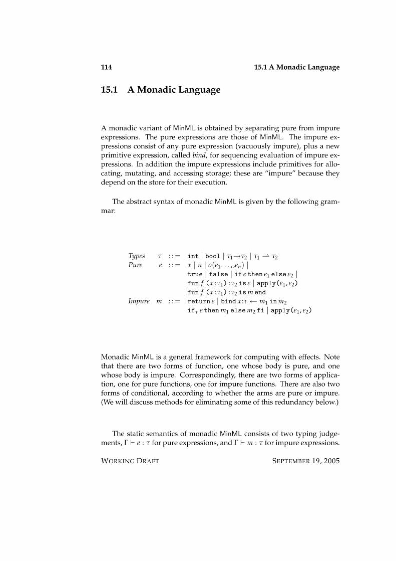
114 15.1 A Monadic Language
15.1 A Monadic Language
A monadic variant of MinML is obtained by separating pure from impureexpressions. The pure expressions are those of MinML. The impure ex-pressions consist of any pure expression (vacuously impure), plus a newprimitive expression, called bind, for sequencing evaluation of impure ex-pressions. In addition the impure expressions include primitives for allo-cating, mutating, and accessing storage; these are “impure” because theydepend on the store for their execution.
The abstract syntax of monadic MinML is given by the following gram-mar:
Types τ : : = int | bool | τ1→τ2 | τ1 τ2Pure e : : = x | n | o(e1. . .,,en) |
true | false | if e then e1 else e2 |fun f (x:τ1):τ2 is e | apply(e1, e2)fun f (x:τ1):τ2 ism end
Impure m : : = return e | bind x:τ ← m1 inm2ifτ e thenm1 elsem2 fi | apply(e1, e2)
Monadic MinML is a general framework for computing with effects. Notethat there are two forms of function, one whose body is pure, and onewhose body is impure. Correspondingly, there are two forms of applica-tion, one for pure functions, one for impure functions. There are also twoforms of conditional, according to whether the arms are pure or impure.(We will discuss methods for eliminating some of this redundancy below.)
The static semantics of monadic MinML consists of two typing judge-ments, Γ ` e : τ for pure expressions, and Γ ` m : τ for impure expressions.
WORKING DRAFT SEPTEMBER 19, 2005
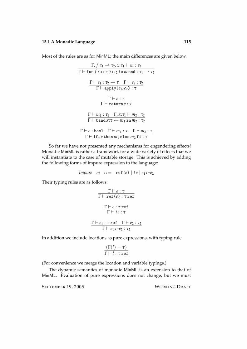
15.1 A Monadic Language 115
Most of the rules are as for MinML; the main differences are given below.
Γ, f :τ1 τ2, x:τ1 ` m : τ2
Γ ` fun f (x:τ1):τ2 ism end : τ1 τ2
Γ ` e1 : τ2 τ Γ ` e2 : τ2
Γ ` apply(e1, e2) : τ
Γ ` e : τΓ ` return e : τ
Γ ` m1 : τ1 Γ, x:τ1 ` m2 : τ2
Γ ` bind x:τ ← m1 inm2 : τ2
Γ ` e : bool Γ ` m1 : τ Γ ` m2 : τ
Γ ` ifτ e thenm1 elsem2 fi : τ
So far we have not presented any mechanisms for engendering effects!Monadic MinML is rather a framework for a wide variety of effects that wewill instantiate to the case of mutable storage. This is achieved by addingthe following forms of impure expression to the language:
Impure m : : = ref(e) | !e | e1:=e2
Their typing rules are as follows:
Γ ` e : τΓ ` ref(e) : τ ref
Γ ` e : τ refΓ ` !e : τ
Γ ` e1 : τ ref Γ ` e2 : τ2
Γ ` e1:=e2 : τ2
In addition we include locations as pure expressions, with typing rule
(Γ(l) = τ)Γ ` l : τ ref
(For convenience we merge the location and variable typings.)The dynamic semantics of monadic MinML is an extension to that of
MinML. Evaluation of pure expressions does not change, but we must
SEPTEMBER 19, 2005 WORKING DRAFT

116 15.2 Reifying Effects
add rules governing evaluation of impure expressions. For the purposesof describing mutable storage, we must consider transitions of the form(M, m) 7→ (M′, m′), where M and M′ are memories, as in Chapter 14.
e 7→ e′
(M, return e) 7→ (M, return e′)
(M, m1) 7→ (M′, m′1)(M, bind x:τ ← m1 inm2) 7→ (M′, bind x:τ ← m′1 inm2)
(M, bind x:τ ← return v inm2) 7→ (M, v/xm2)
The evaluation rules for the reference primitives are as in Chapter 14.
15.2 Reifying Effects
The need for pure and impure function spaces in monadic MinML is some-what unpleasant because of the duplication of constructs. One way toavoid this is to introduce a new type constructor, ! τ, whose elements areunevaluated impure expressions. The computation embodied by the ex-pression is said to be reified (turned into a “thing”).
The syntax required for this extension is as follows:
Types τ : : = ! τPure e : : = box(m)Impure m : : = unbox(e)
Informally, the pure expression box(m) is a value that contains an un-evaluated impure expression m; the expression m is said to be boxed. Boxedexpressions can be used as ordinary values without restriction. The expres-sion unbox(e) “opens the box” and evaluates the impure expression inside;it is therefore itself an impure expression.
The static semantics of this extension is given by the following rules:
Γ ` m : τΓ ` box(m) : ! τ
Γ ` e : ! τΓ ` unbox(e) : τ
WORKING DRAFT SEPTEMBER 19, 2005
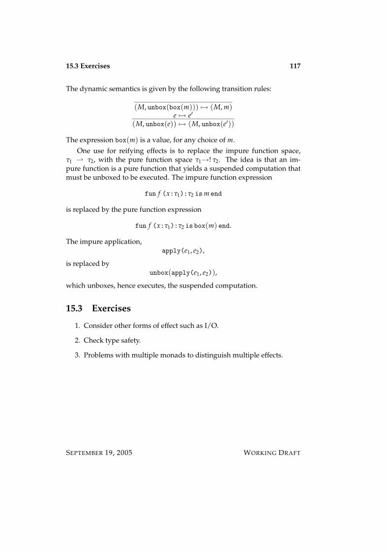
15.3 Exercises 117
The dynamic semantics is given by the following transition rules:
(M, unbox(box(m))) 7→ (M, m)e 7→ e′
(M, unbox(e)) 7→ (M, unbox(e′))
The expression box(m) is a value, for any choice of m.One use for reifying effects is to replace the impure function space,
τ1 τ2, with the pure function space τ1→! τ2. The idea is that an im-pure function is a pure function that yields a suspended computation thatmust be unboxed to be executed. The impure function expression
fun f (x:τ1):τ2 ism end
is replaced by the pure function expression
fun f (x:τ1):τ2 is box(m) end.
The impure application,apply(e1, e2),
is replaced byunbox(apply(e1, e2)),
which unboxes, hence executes, the suspended computation.
15.3 Exercises
1. Consider other forms of effect such as I/O.
2. Check type safety.
3. Problems with multiple monads to distinguish multiple effects.
SEPTEMBER 19, 2005 WORKING DRAFT

118 15.3 Exercises
WORKING DRAFT SEPTEMBER 19, 2005
Part VI
Cost Semantics and Parallelism
119

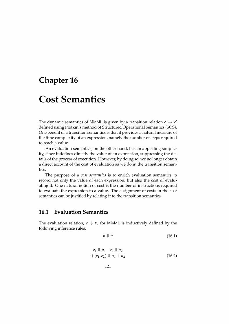
Chapter 16
Cost Semantics
The dynamic semantics of MinML is given by a transition relation e 7→ e′
defined using Plotkin’s method of Structured Operational Semantics (SOS).One benefit of a transition semantics is that it provides a natural measure ofthe time complexity of an expression, namely the number of steps requiredto reach a value.
An evaluation semantics, on the other hand, has an appealing simplic-ity, since it defines directly the value of an expression, suppressing the de-tails of the process of execution. However, by doing so, we no longer obtaina direct account of the cost of evaluation as we do in the transition seman-tics.
The purpose of a cost semantics is to enrich evaluation semantics torecord not only the value of each expression, but also the cost of evalu-ating it. One natural notion of cost is the number of instructions requiredto evaluate the expression to a value. The assignment of costs in the costsemantics can be justified by relating it to the transition semantics.
16.1 Evaluation Semantics
The evaluation relation, e ⇓ v, for MinML is inductively defined by thefollowing inference rules.
n ⇓ n (16.1)
e1 ⇓ n1 e2 ⇓ n2
+(e1, e2) ⇓ n1 + n2 (16.2)
121
122 16.2 Relating Evaluation Semantics to Transition Semantics
(and similarly for the other primitive operations).
true ⇓ true false ⇓ false (16.3)
e ⇓ true e1 ⇓ vif e then e1 else e2 ⇓ v (16.4)
e ⇓ false e2 ⇓ vif e then e1 else e2 ⇓ v (16.5)
fun f (x:τ1):τ2 is e ⇓ fun f (x:τ1):τ2 is e (16.6)
e1 ⇓ v1 e2 ⇓ v2 v1, v2/ f , xe ⇓ vapply(e1, e2) ⇓ v (16.7)
(where v1 = fun f (x:τ1):τ2 is e.)This concludes the definition of the evaluation semantics of MinML. As
you can see, the specification is quite small and is very intuitively appeal-ing.
16.2 Relating Evaluation Semantics to Transition Se-mantics
The precise relationship between SOS and ES is given by the following the-orem.
Theorem 16.11. If e ⇓ v, then e 7→∗ v.
2. If e 7→ e′ and e′ ⇓ v, then e ⇓ v. Consequently, if e 7→∗ v, then e ⇓ v.
Proof:
1. By induction on the rules defining the evaluation relation. The re-sult is clearly true for values, since trivially v 7→∗ v. Suppose thate = apply(e1, e2) and assume that e ⇓ v. Then e1 ⇓ v1, wherev1 = fun f (x:τ1):τ2 is e, e2 ⇓ v2, and v1, v2/ f , xe ⇓ v. By in-duction we have that e1 7→∗ v1, e2 7→∗ v2 and v1, v2/ f , xe 7→∗ v.It follows that apply(e1, e2) 7→∗ apply(v1, e2) 7→∗ apply(v1, v2) 7→v1, v2/ f , xe 7→∗ v, as required. The other cases are handled simi-larly.
WORKING DRAFT SEPTEMBER 19, 2005

16.3 Cost Semantics 123
2. By induction on the rules defining single-step transition. Supposethat e = apply(v1, v2), where v1 = fun f (x:τ1):τ2 is e, and e′ =v1, v2/ f , xe. Suppose further that e′ ⇓ v; we are to show that e ⇓ v.Since v1 ⇓ v1 and v2 ⇓ v2, the result follows immediately from theassumption that e′ ⇓ v. Now suppose that e = apply(e1, e2) ande′ = apply(e′1, e2), where e1 7→ e′1. Assume that e′ ⇓ v; we are toshow that e ⇓ v. It follows that e′1 ⇓ v1, e2 ⇓ v2, and v1, v2/ f , xe ⇓v. By induction e1 ⇓ v1, and hence e ⇓ v. The remaining cases arehandled similarly. It follows by induction on the rules defining multi-step evaluation that if e 7→∗ v, then e ⇓ v. The base case, v 7→∗ v,follows from the fact that v ⇓ v. Now suppose that e 7→ e′ 7→∗ v. Byinduction e′ ⇓ v, and hence e ⇓ v by what we have just proved.
16.3 Cost Semantics
In this section we will give a cost semantics for MinML that reflects thenumber of steps required to complete evaluation according to the struc-tured operational semantics given in Chapter 9.
Evaluation judgements have the form e ⇓n v, with the informal mean-ing that e evaluates to v in n steps. The rules for deriving these judgementsare easily defined.
n ⇓0 n (16.8)
e1 ⇓k1 n1 e2 ⇓k2 n2
+(e1, e2) ⇓k1+k2+1 n1 + n2 (16.9)
(and similarly for the other primitive operations).
true ⇓0 true false ⇓0 false (16.10)
e ⇓k true e1 ⇓k1 vif e then e1 else e2 ⇓k+k1+1 v (16.11)
e ⇓k false e2 ⇓k2 vif e then e1 else e2 ⇓k+k2+1 v (16.12)
SEPTEMBER 19, 2005 WORKING DRAFT
124 16.4 Relating Cost Semantics to Transition Semantics
fun f (x:τ1):τ2 is e ⇓0 fun f (x:τ1):τ2 is e (16.13)
e1 ⇓k1 v1 e2 ⇓k2 v2 v1, v2/ f , xe ⇓k v
apply(e1, e2) ⇓k1+k2+k+1 v (16.14)
(where v1 = fun f (x:τ1):τ2 is e.)This completes the definition of the cost semantics for MinML.
16.4 Relating Cost Semantics to Transition Semantics
What is it that makes the cost semantics given above “correct”? Informally,we expect that if e ⇓k v, then e should evaluate to v in k steps. Moreover,we also expect the converse to hold — the cost semantics should be com-pletely faithful to the underlying execution model. This is captured by thefollowing theorem.
To state the theorem we need one additional bit of notation. Definee k7→ e′ by induction on k as follows. For the basis, we define e 07→ e′ iff
e = e′; if k = k′ + 1, we define e k7→ e′ to hold iff e 7→ e′′ k′7→ e′.
Theorem 16.2For any closed expression e and closed value v of the same type, e ⇓k v iff
e k7→ v.
Proof: From left to right we proceed by induction on the definition of thecost semantics. For example, consider the rule for function application. Wehave e = apply(e1, e2) and k = k1 + k2 + k + 1, where
1. e1 ⇓k1 v1,
2. e2 ⇓k2 v2,
3. v1 = fun f (x:τ1):τ2 is e,
4. v1, v2/ f , xe ⇓k v.
By induction we have
1. e1k17→ v1,
2. e2k27→ v2,
WORKING DRAFT SEPTEMBER 19, 2005

16.5 Exercises 125
3. v1, v2/ f , xe k7→ v,
and hencee1(e2)
k17→ v1(e2)k27→ v1(v2)7→ v1, v2/ f , xe
k7→ v
which is enough for the result.From right to left we proceed by induction on k. For k = 0, we must
have e = v. By inspection of the cost evaluation rules we may check thatv ⇓0 v for every value v. For k = k′ + 1, we must show that if e 7→ e′
and e′ ⇓k′ v, then e ⇓k v. This is proved by a subsidiary induction on thetransition rules. For example, suppose that e = e1(e2) 7→ e′1(e2) = e′, withe1 7→ e′1. By hypothesis e′1(e2) ⇓k v, so k = k1 + k2 + k3 + 1, where
1. e′1 ⇓k1 v1,
2. e2 ⇓k2 v2,
3. v1 = fun f (x:τ1):τ2 is e,
4. v1, v2/ f , xe ⇓k3 v.
By induction e1 ⇓k1+1 v1, hence e ⇓k+1 v, as required.
16.5 Exercises
SEPTEMBER 19, 2005 WORKING DRAFT

126 16.5 Exercises
WORKING DRAFT SEPTEMBER 19, 2005
Chapter 17
Implicit Parallelism
In this chapter we study the extension of MinML with implicit data paral-lelism, a means of speeding up computations by allowing expressions tobe evaluated simultaneously. By “implicit” we mean that the use of paral-lelism is invisible to the programmer as far as the ultimate results of com-putation are concerned. By “data parallel” we mean that the parallelism ina program arises from the simultaneous evaluation of the components of adata structure.
Implicit parallelism is very natural in an effect-free language such asMinML. The reason is that in such a language it is not possible to deter-mine the order in which the components of an aggregate data structureare evaluated. They might be evaluated in an arbitrary sequential order,or might even be evaluated simultaneously, without affecting the outcomeof the computation. This is in sharp contrast to effect-ful languages, forthen the order of evaluation, or the use of parallelism, is visible to the pro-grammer. Indeed, dependence on the evaluation order must be carefullyguarded against to ensure that the outcome is determinate.
17.1 Tuple Parallelism
We begin by considering a parallel semantics for tuples according to whichall components of a tuple are evaluated simultaneously. For simplicity weconsider only pairs, but the ideas generalize in a straightforward mannerto tuples of any size. Since the “widths” of tuples are specified statically aspart of their type, the amount of parallelism that can be induced in any onestep is bounded by a static constant. In Section 17.3 we will extend this topermit a statically unbounded degree of parallelism.
127
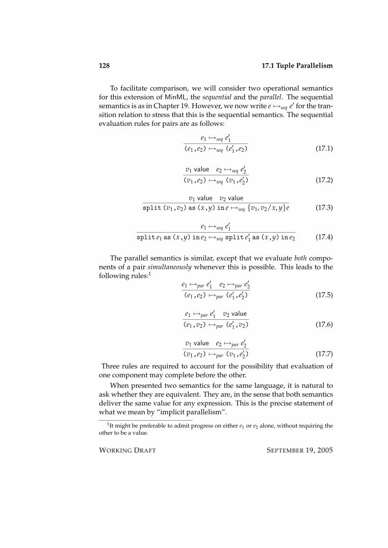
128 17.1 Tuple Parallelism
To facilitate comparison, we will consider two operational semanticsfor this extension of MinML, the sequential and the parallel. The sequentialsemantics is as in Chapter 19. However, we now write e 7→seq e′ for the tran-sition relation to stress that this is the sequential semantics. The sequentialevaluation rules for pairs are as follows:
e1 7→seq e′1(e1,e2) 7→seq (e′1,e2) (17.1)
v1 value e2 7→seq e′2(v1,e2) 7→seq (v1,e′2) (17.2)
v1 value v2 value
split (v1,v2) as (x,y) in e 7→seq v1, v2/x, ye (17.3)
e1 7→seq e′1split e1 as (x,y) in e2 7→seq split e′1 as (x,y) in e2 (17.4)
The parallel semantics is similar, except that we evaluate both compo-nents of a pair simultaneously whenever this is possible. This leads to thefollowing rules:1
e1 7→par e′1 e2 7→par e′2(e1,e2) 7→par (e′1,e′2) (17.5)
e1 7→par e′1 v2 value
(e1,v2) 7→par (e′1,v2) (17.6)
v1 value e2 7→par e′2(v1,e2) 7→par (v1,e′2) (17.7)
Three rules are required to account for the possibility that evaluation ofone component may complete before the other.
When presented two semantics for the same language, it is natural toask whether they are equivalent. They are, in the sense that both semanticsdeliver the same value for any expression. This is the precise statement ofwhat we mean by “implicit parallelism”.
1It might be preferable to admit progress on either e1 or e2 alone, without requiring theother to be a value.
WORKING DRAFT SEPTEMBER 19, 2005
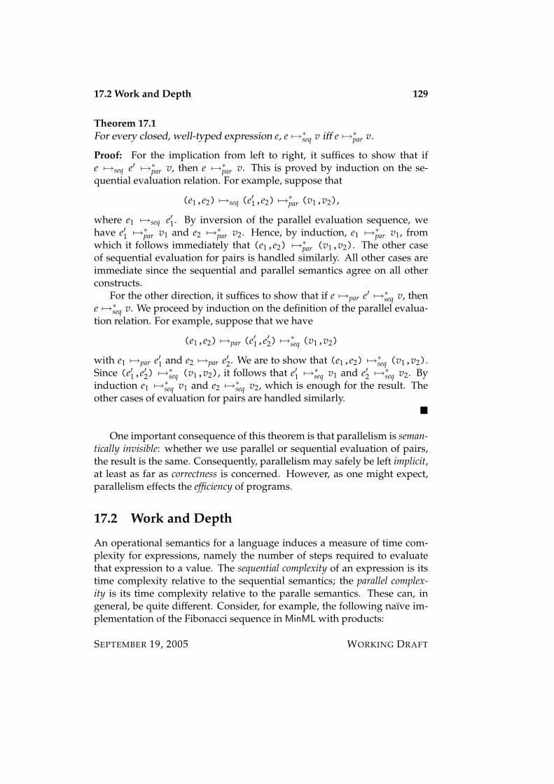
17.2 Work and Depth 129
Theorem 17.1For every closed, well-typed expression e, e 7→∗seq v iff e 7→∗par v.
Proof: For the implication from left to right, it suffices to show that ife 7→seq e′ 7→∗par v, then e 7→∗par v. This is proved by induction on the se-quential evaluation relation. For example, suppose that
(e1,e2) 7→seq (e′1,e2) 7→∗par (v1,v2),
where e1 7→seq e′1. By inversion of the parallel evaluation sequence, wehave e′1 7→∗par v1 and e2 7→∗par v2. Hence, by induction, e1 7→∗par v1, fromwhich it follows immediately that (e1,e2) 7→∗par (v1,v2). The other caseof sequential evaluation for pairs is handled similarly. All other cases areimmediate since the sequential and parallel semantics agree on all otherconstructs.
For the other direction, it suffices to show that if e 7→par e′ 7→∗seq v, thene 7→∗seq v. We proceed by induction on the definition of the parallel evalua-tion relation. For example, suppose that we have
(e1,e2) 7→par (e′1,e′2) 7→∗seq (v1,v2)
with e1 7→par e′1 and e2 7→par e′2. We are to show that (e1,e2) 7→∗seq (v1,v2).Since (e′1,e′2) 7→∗seq (v1,v2), it follows that e′1 7→∗seq v1 and e′2 7→∗seq v2. Byinduction e1 7→∗seq v1 and e2 7→∗seq v2, which is enough for the result. Theother cases of evaluation for pairs are handled similarly.
One important consequence of this theorem is that parallelism is seman-tically invisible: whether we use parallel or sequential evaluation of pairs,the result is the same. Consequently, parallelism may safely be left implicit,at least as far as correctness is concerned. However, as one might expect,parallelism effects the efficiency of programs.
17.2 Work and Depth
An operational semantics for a language induces a measure of time com-plexity for expressions, namely the number of steps required to evaluatethat expression to a value. The sequential complexity of an expression is itstime complexity relative to the sequential semantics; the parallel complex-ity is its time complexity relative to the paralle semantics. These can, ingeneral, be quite different. Consider, for example, the following naıve im-plementation of the Fibonacci sequence in MinML with products:
SEPTEMBER 19, 2005 WORKING DRAFT
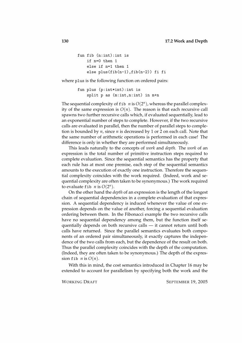
130 17.2 Work and Depth
fun fib (n:int):int isif n=0 then 1else if n=1 then 1else plus(fib(n-1),fib(n-2)) fi fi
where plus is the following function on ordered pairs:
fun plus (p:int*int):int issplit p as (m:int,n:int) in m+n
The sequential complexity of fib n is O(2n), whereas the parallel complex-ity of the same expression is O(n). The reason is that each recursive callspawns two further recursive calls which, if evaluated sequentially, lead toan exponential number of steps to complete. However, if the two recursivecalls are evaluated in parallel, then the number of parallel steps to comple-tion is bounded by n, since n is decreased by 1 or 2 on each call. Note thatthe same number of arithmetic operations is performed in each case! Thedifference is only in whether they are performed simultaneously.
This leads naturally to the concepts of work and depth. The work of anexpression is the total number of primitive instruction steps required tocomplete evaluation. Since the sequential semantics has the property thateach rule has at most one premise, each step of the sequential semanticsamounts to the execution of exactly one instruction. Therefore the sequen-tial complexity coincides with the work required. (Indeed, work and se-quential complexity are often taken to be synonymous.) The work requiredto evaluate fib n is O(2n).
On the other hand the depth of an expression is the length of the longestchain of sequential dependencies in a complete evaluation of that expres-sion. A sequential dependency is induced whenever the value of one ex-pression depends on the value of another, forcing a sequential evaluationordering between them. In the Fibonacci example the two recursive callshave no sequential dependency among them, but the function itself se-quentially depends on both recursive calls — it cannot return until bothcalls have returned. Since the parallel semantics evaluates both compo-nents of an ordered pair simultaneously, it exactly captures the indepen-dence of the two calls from each, but the dependence of the result on both.Thus the parallel complexity coincides with the depth of the computation.(Indeed, they are often taken to be synonymous.) The depth of the expres-sion fib n is O(n).
With this in mind, the cost semantics introduced in Chapter 16 may beextended to account for parallelism by specifying both the work and the
WORKING DRAFT SEPTEMBER 19, 2005
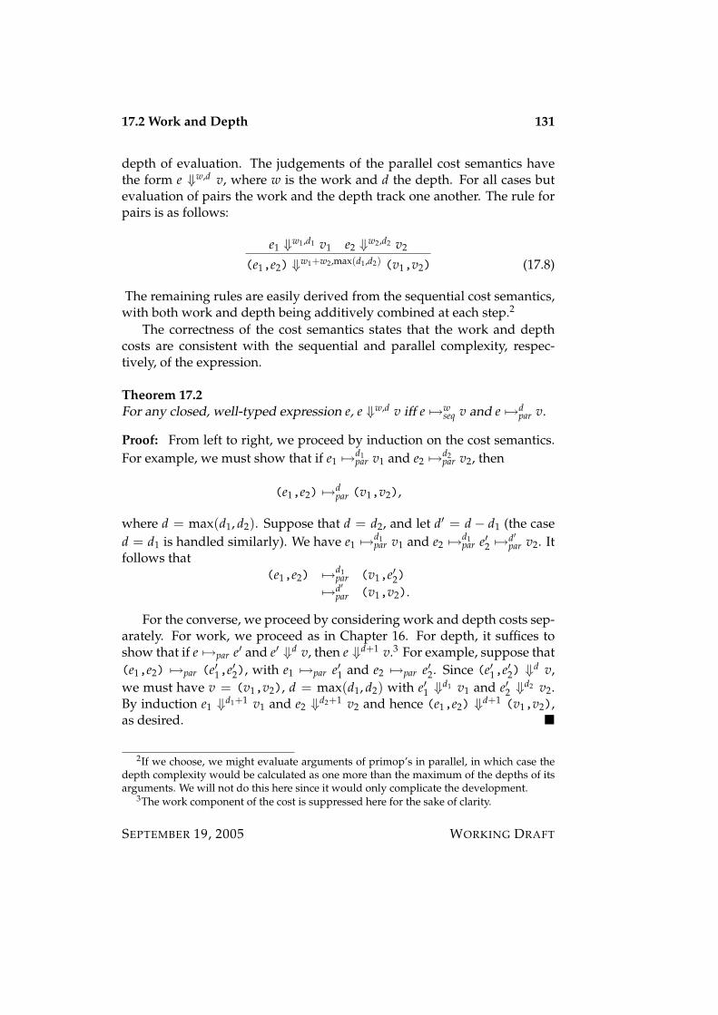
17.2 Work and Depth 131
depth of evaluation. The judgements of the parallel cost semantics havethe form e ⇓w,d v, where w is the work and d the depth. For all cases butevaluation of pairs the work and the depth track one another. The rule forpairs is as follows:
e1 ⇓w1,d1 v1 e2 ⇓w2,d2 v2
(e1,e2) ⇓w1+w2,max(d1,d2) (v1,v2) (17.8)
The remaining rules are easily derived from the sequential cost semantics,with both work and depth being additively combined at each step.2
The correctness of the cost semantics states that the work and depthcosts are consistent with the sequential and parallel complexity, respec-tively, of the expression.
Theorem 17.2For any closed, well-typed expression e, e ⇓w,d v iff e 7→w
seq v and e 7→dpar v.
Proof: From left to right, we proceed by induction on the cost semantics.For example, we must show that if e1 7→d1
par v1 and e2 7→d2par v2, then
(e1,e2) 7→dpar (v1,v2),
where d = max(d1, d2). Suppose that d = d2, and let d′ = d− d1 (the cased = d1 is handled similarly). We have e1 7→d1
par v1 and e2 7→d1par e′2 7→d′
par v2. Itfollows that
(e1,e2) 7→d1par (v1,e′2)
7→d′par (v1,v2).
For the converse, we proceed by considering work and depth costs sep-arately. For work, we proceed as in Chapter 16. For depth, it suffices toshow that if e 7→par e′ and e′ ⇓d v, then e ⇓d+1 v.3 For example, suppose that(e1,e2) 7→par (e′1,e′2), with e1 7→par e′1 and e2 7→par e′2. Since (e′1,e′2) ⇓d v,we must have v = (v1,v2), d = max(d1, d2) with e′1 ⇓d1 v1 and e′2 ⇓d2 v2.By induction e1 ⇓d1+1 v1 and e2 ⇓d2+1 v2 and hence (e1,e2) ⇓d+1 (v1,v2),as desired.
2If we choose, we might evaluate arguments of primop’s in parallel, in which case thedepth complexity would be calculated as one more than the maximum of the depths of itsarguments. We will not do this here since it would only complicate the development.
3The work component of the cost is suppressed here for the sake of clarity.
SEPTEMBER 19, 2005 WORKING DRAFT
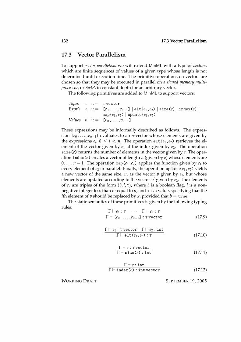
132 17.3 Vector Parallelism
17.3 Vector Parallelism
To support vector parallelism we will extend MinML with a type of vectors,which are finite sequences of values of a given type whose length is notdetermined until execution time. The primitive operations on vectors arechosen so that they may be executed in parallel on a shared memory multi-processor, or SMP, in constant depth for an arbitrary vector.
The following primitives are added to MinML to support vectors:
Types τ : : = τ vectorExpr’s e : : = [e0, . . . ,en−1] | elt(e1,e2) | size(e) | index(e) |
map(e1,e2) | update(e1,e2)Values v : : = [v0, . . . ,vn−1]
These expressions may be informally described as follows. The expres-sion [e0, . . . ,en−1] evaluates to an n-vector whose elements are given bythe expressions ei, 0 ≤ i < n. The operation elt(e1,e2) retrieves the el-ement of the vector given by e1 at the index given by e2. The operationsize(e) returns the number of elements in the vector given by e. The oper-ation index(e) creates a vector of length n (given by e) whose elements are0, . . . , n− 1. The operation map(e1,e2) applies the function given by e1 toevery element of e2 in parallel. Finally, the operation update(e1,e2) yieldsa new vector of the same size, n, as the vector v given by e1, but whoseelements are updated according to the vector v′ given by e2. The elementsof e2 are triples of the form (b, i, x), where b is a boolean flag, i is a non-negative integer less than or equal to n, and x is a value, specifying that theith element of v should be replaced by x, provided that b = true.
The static semantics of these primitives is given by the following typingrules:
Γ ` e1 : τ · · · Γ ` en : τ
Γ ` [e0, . . . ,en−1] : τ vector (17.9)
Γ ` e1 : τ vector Γ ` e2 : intΓ ` elt(e1,e2) : τ (17.10)
Γ ` e : τ vectorΓ ` size(e) : int (17.11)
Γ ` e : intΓ ` index(e) : int vector (17.12)
WORKING DRAFT SEPTEMBER 19, 2005
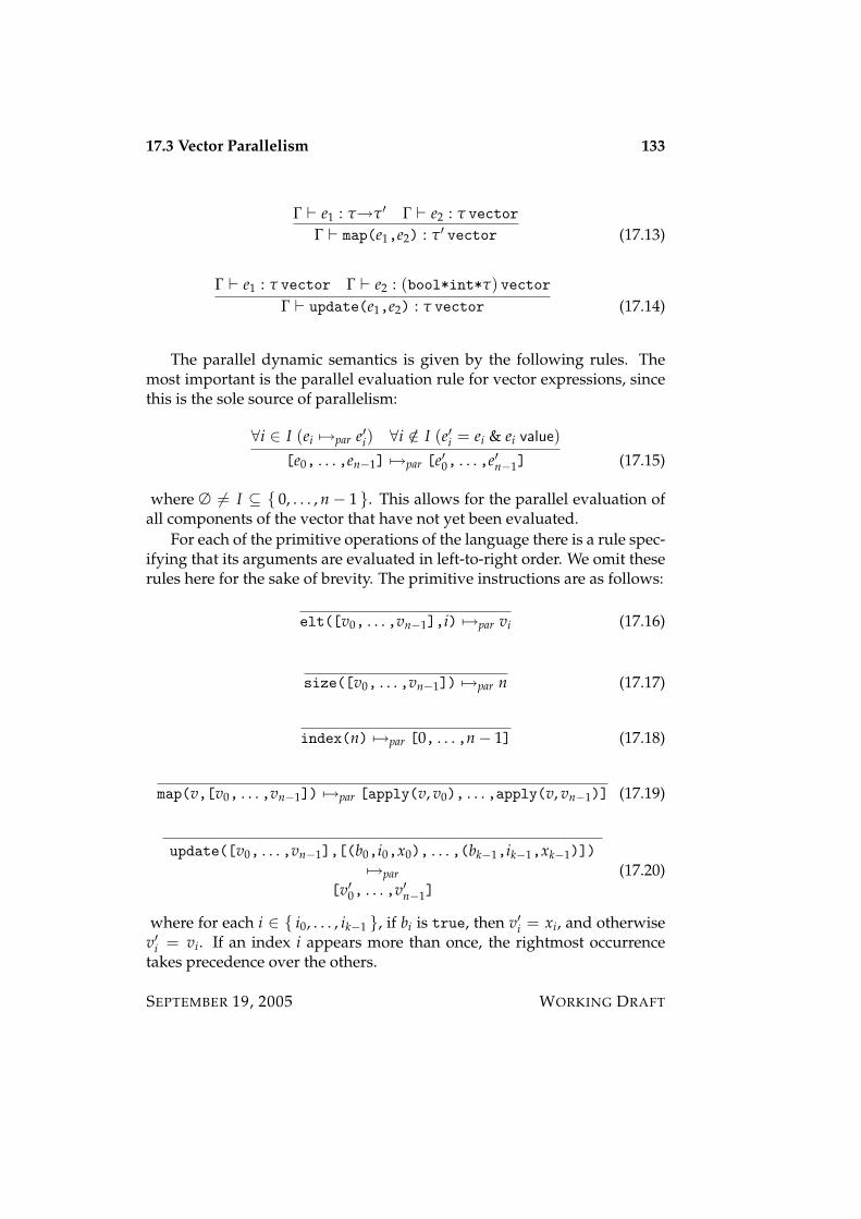
17.3 Vector Parallelism 133
Γ ` e1 : τ→τ′ Γ ` e2 : τ vector
Γ ` map(e1,e2) : τ′ vector (17.13)
Γ ` e1 : τ vector Γ ` e2 : (bool*int*τ) vectorΓ ` update(e1,e2) : τ vector (17.14)
The parallel dynamic semantics is given by the following rules. Themost important is the parallel evaluation rule for vector expressions, sincethis is the sole source of parallelism:
∀i ∈ I (ei 7→par e′i) ∀i /∈ I (e′i = ei & ei value)[e0, . . . ,en−1] 7→par [e′0, . . . ,e′n−1] (17.15)
where ∅ 6= I ⊆ 0, . . . , n− 1 . This allows for the parallel evaluation ofall components of the vector that have not yet been evaluated.
For each of the primitive operations of the language there is a rule spec-ifying that its arguments are evaluated in left-to-right order. We omit theserules here for the sake of brevity. The primitive instructions are as follows:
elt([v0, . . . ,vn−1],i) 7→par vi (17.16)
size([v0, . . . ,vn−1]) 7→par n (17.17)
index(n) 7→par [0, . . . ,n− 1] (17.18)
map(v,[v0, . . . ,vn−1]) 7→par [apply(v, v0), . . . ,apply(v, vn−1)] (17.19)
update([v0, . . . ,vn−1],[(b0,i0,x0), . . . ,(bk−1,ik−1,xk−1)])7→par
[v′0, . . . ,v′n−1](17.20)
where for each i ∈ i0, . . . , ik−1 , if bi is true, then v′i = xi, and otherwisev′i = vi. If an index i appears more than once, the rightmost occurrencetakes precedence over the others.
SEPTEMBER 19, 2005 WORKING DRAFT
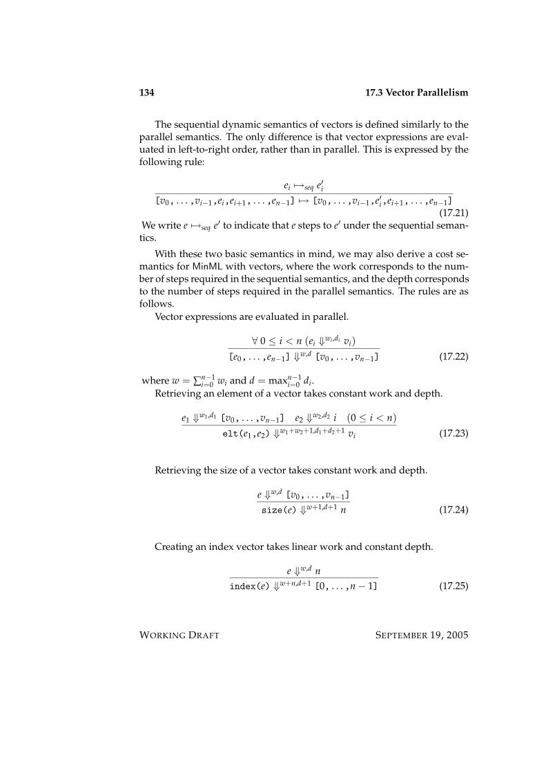
134 17.3 Vector Parallelism
The sequential dynamic semantics of vectors is defined similarly to theparallel semantics. The only difference is that vector expressions are eval-uated in left-to-right order, rather than in parallel. This is expressed by thefollowing rule:
ei 7→seq e′i[v0, . . . ,vi−1,ei,ei+1, . . . ,en−1] 7→ [v0, . . . ,vi−1,e′i,ei+1, . . . ,en−1]
(17.21)We write e 7→seq e′ to indicate that e steps to e′ under the sequential seman-tics.
With these two basic semantics in mind, we may also derive a cost se-mantics for MinML with vectors, where the work corresponds to the num-ber of steps required in the sequential semantics, and the depth correspondsto the number of steps required in the parallel semantics. The rules are asfollows.
Vector expressions are evaluated in parallel.
∀ 0 ≤ i < n (ei ⇓wi ,di vi)[e0, . . . ,en−1] ⇓w,d [v0, . . . ,vn−1] (17.22)
where w = ∑n−1i=0 wi and d = maxn−1
i=0 di.Retrieving an element of a vector takes constant work and depth.
e1 ⇓w1,d1 [v0, . . . ,vn−1] e2 ⇓w2,d2 i (0 ≤ i < n)elt(e1,e2) ⇓w1+w2+1,d1+d2+1 vi (17.23)
Retrieving the size of a vector takes constant work and depth.
e ⇓w,d [v0, . . . ,vn−1]
size(e) ⇓w+1,d+1 n (17.24)
Creating an index vector takes linear work and constant depth.
e ⇓w,d nindex(e) ⇓w+n,d+1 [0, . . . ,n− 1] (17.25)
WORKING DRAFT SEPTEMBER 19, 2005

17.3 Vector Parallelism 135
Mapping a function across a vector takes constant work and depth be-yond the cost of the function applications.
e1 ⇓w1,d1 v e2 ⇓w2,d2 [v0, . . . ,vn−1][apply(v, v0), . . . ,apply(v, vn−1)] ⇓w,d [v′0, . . . ,v′n−1]
map(e1,e2) ⇓w1+w2+w+1,d1+d2+d+1 [v′0, . . . ,v′n−1] (17.26)
Updating a vector takes linear work and constant depth.
e1 ⇓w1,d1 [v0, . . . ,vn−1] e2 ⇓w2,d2 [(b1,i1,x1), . . . ,(bk,ik,xk)]
update(e1,e2) ⇓w1+w2+k+n,d1+d2+1 [v′0, . . . ,v′n−1] (17.27)
where for each i ∈ i1, . . . , ik , if bi is true, then v′i = xi, and otherwisev′i = vi. If an index i appears more than once, the rightmost occurrencetakes precedence over the others.
Theorem 17.3For the extension of MinML with vectors, e ⇓w,d v iff e 7→d
par v and e 7→wseq v.
SEPTEMBER 19, 2005 WORKING DRAFT

136 17.3 Vector Parallelism
WORKING DRAFT SEPTEMBER 19, 2005
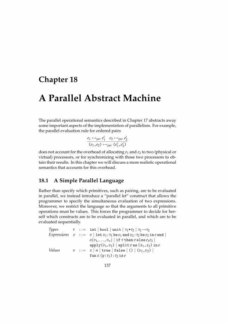
Chapter 18
A Parallel Abstract Machine
The parallel operational semantics described in Chapter 17 abstracts awaysome important aspects of the implementation of parallelism. For example,the parallel evaluation rule for ordered pairs
e1 7→par e′1 e2 7→par e′2(e1,e2) 7→par (e′1,e′2)
does not account for the overhead of allocating e1 and e2 to two (physical orvirtual) processors, or for synchronizing with those two processors to ob-tain their results. In this chapter we will discuss a more realistic operationalsemantics that accounts for this overhead.
18.1 A Simple Parallel Language
Rather than specify which primitives, such as pairing, are to be evaluatedin parallel, we instead introduce a “parallel let” construct that allows theprogrammer to specify the simultaneous evaluation of two expressions.Moreover, we restrict the language so that the arguments to all primitiveoperations must be values. This forces the programmer to decide for her-self which constructs are to be evaluated in parallel, and which are to beevaluated sequentially.
Types τ : : = int | bool | unit | τ1*τ2 | τ1→τ2Expressions e : : = v | let x1:τ1 be e1 and x2:τ2 be e2 in e end |
o(v1, . . . , vn) | if τ then v else e1e2 |apply(v1, v2) | split v as (x1,x2) in e
Values v : : = x | n | true | false | () | (v1,v2) |fun x (y:τ1):τ2 is e
137

138 18.1 A Simple Parallel Language
The binding conventions are as for MinML with product types, with theadditional specification that the variables x1 and x2 are bound within thebody of a let expression. Note that variables are regarded as values onlyfor the purpose of defining the syntax of the language; evaluation is, asever, defined only on closed terms.
As will become apparent when we specify the dynamic semantics, the“sequential let” is definable from the “parallel let”:
let τ1:x1 be e1 in e2 : = let x1:τ1 be e1 and x:unit be () in e2 end
where x does not occur free in e2. Using these, the “parallel pair” is defin-able by the equation
(e1,e2)par : = let x1:τ1 be e1 and x2:τ2 be e2 in (x1,x2) end
whereas the “(left-to-right) sequential pair” is definable by the equation
(e1,e2)seq : = let τ1:x1 be e1 in let τ2:x2 be e2 in (x1,x2).
The static semantics of this language is essentially that of MinML withproduct types, with the addition of the following typing rule for the parallellet construct:
Γ ` e1 : τ1 Γ ` e2 : τ2 Γ, x1:τ1, x2:τ2 ` e : τ
Γ ` let x1:τ1 be e1 and x2:τ2 be e2 in e end : τ (18.1)
It is a simple exercise to give a parallel structured operational semanticsto this language in the style of Chapter 17. In particular, it would employthe following rules for the parallel let construct.
e1 7→par e′1 e2 7→par e′2let x1:τ1 be e1 and x2:τ2 be e2 in e end
7→parlet x1:τ1 be e′1 and x2:τ2 be e′2 in e end
(18.2)
e1 7→par e′1let x1:τ1 be e1 and x2:τ2 be v2 in e end
7→parlet x1:τ1 be e′1 and x2:τ2 be v2 in e end
(18.3)
WORKING DRAFT SEPTEMBER 19, 2005
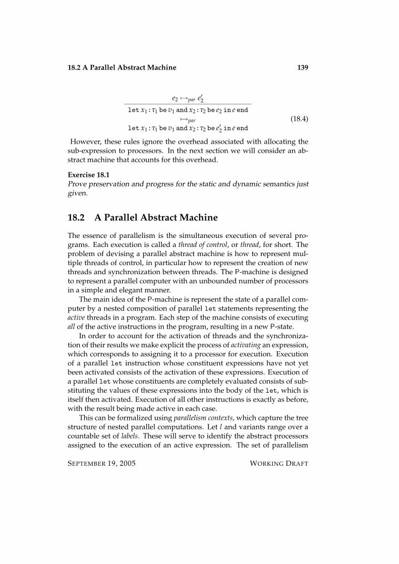
18.2 A Parallel Abstract Machine 139
e2 7→par e′2let x1:τ1 be v1 and x2:τ2 be e2 in e end
7→parlet x1:τ1 be v1 and x2:τ2 be e′2 in e end
(18.4)
However, these rules ignore the overhead associated with allocating thesub-expression to processors. In the next section we will consider an ab-stract machine that accounts for this overhead.
Exercise 18.1Prove preservation and progress for the static and dynamic semantics justgiven.
18.2 A Parallel Abstract Machine
The essence of parallelism is the simultaneous execution of several pro-grams. Each execution is called a thread of control, or thread, for short. Theproblem of devising a parallel abstract machine is how to represent mul-tiple threads of control, in particular how to represent the creation of newthreads and synchronization between threads. The P-machine is designedto represent a parallel computer with an unbounded number of processorsin a simple and elegant manner.
The main idea of the P-machine is represent the state of a parallel com-puter by a nested composition of parallel let statements representing theactive threads in a program. Each step of the machine consists of executingall of the active instructions in the program, resulting in a new P-state.
In order to account for the activation of threads and the synchroniza-tion of their results we make explicit the process of activating an expression,which corresponds to assigning it to a processor for execution. Executionof a parallel let instruction whose constituent expressions have not yetbeen activated consists of the activation of these expressions. Execution ofa parallel let whose constituents are completely evaluated consists of sub-stituting the values of these expressions into the body of the let, which isitself then activated. Execution of all other instructions is exactly as before,with the result being made active in each case.
This can be formalized using parallelism contexts, which capture the treestructure of nested parallel computations. Let l and variants range over acountable set of labels. These will serve to identify the abstract processorsassigned to the execution of an active expression. The set of parallelism
SEPTEMBER 19, 2005 WORKING DRAFT

140 18.2 A Parallel Abstract Machine
contexts L is defined by the following grammar:
L : : = l: | l:let x1:τ1 beL1 and x2:τ2 beL2 in e end |l:let x1:τ1 beL1 and x2:τ2 be v2 in e end |
l:let x1:τ1 be v1 and x2:τ2 beL2 in e end
A parallelism context is well-formed only if all labels occurring within it aredistinct; hereafter we will consider only well-formed parallelism contexts.
A labelled “hole” in a parallelism context represents an active computa-tion site; a labelled let expression represents a pending computation thatis awaiting completion of its child threads. We have arranged things so thatall active sites are children of pending sites, reflecting the intuition that anactive site must have been spawned by some (now pending) site.
The arity of a context is defined to be the number of “holes” occurringwithin it. The arity is therefore the number of active threads within thecontext. If L is a context with arity n, then the expression L[l = e]ni=1 rep-resents the result of “filling” the hole labelled li with the expression ei, foreach 1 ≤ i ≤ n. Thus the ei’s represent the active expressions within thecontext; the label li represents the “name” of the processor assigned to exe-cute ei.
Each step of the P-machine consists of executing all of the active instruc-tions in the current state. This is captured by the following evaluation rule:
e1 −→ e′1 · · · en −→ e′nL[l = e]ni=1 7→P L[l = e′]ni=1
The relation e −→ e′ defines the atomic instruction steps of the P-machine. These are defined by a set of axioms. The first is the fork axiom,which initiates execution of a parallel let statement:
let x1:τ1 be e1 and x2:τ2 be e2 in e end−→
let x1:τ1 be l1:e1 and x2:τ2 be l2:e2 in e end(18.5)
Here l1 and l2 are “new” labels that do not otherwise occur in the compu-tation. They serve as the labels of the processors assigned to execute e1 ande2, respectively.
The second instruction is the join axiom, which completes execution ofa parallel let:
v1 value v2 value
let x1:τ1 be l1:v1 and x2:τ2 be l2:v2 in e end −→ v1, v2/x1, x2e (18.6)
WORKING DRAFT SEPTEMBER 19, 2005
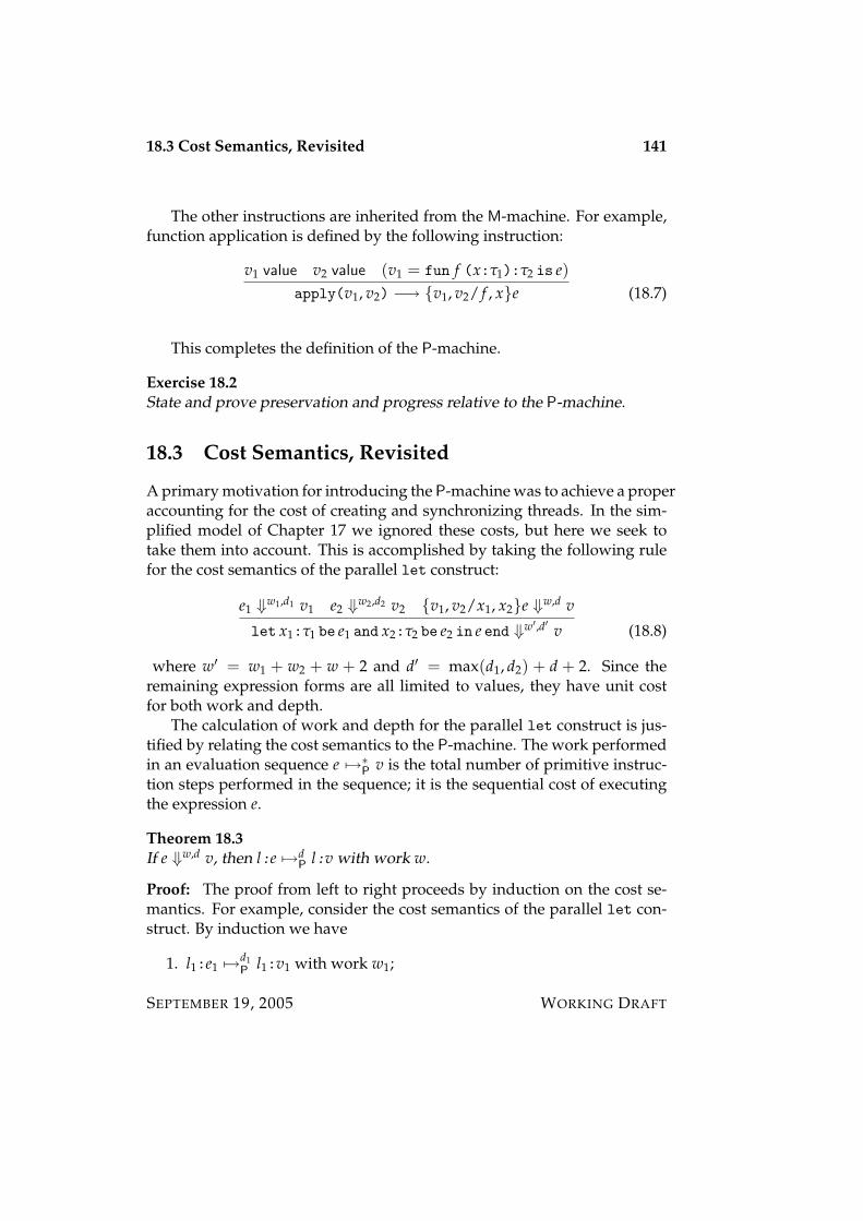
18.3 Cost Semantics, Revisited 141
The other instructions are inherited from the M-machine. For example,function application is defined by the following instruction:
v1 value v2 value (v1 = fun f (x:τ1):τ2 is e)apply(v1, v2) −→ v1, v2/ f , xe (18.7)
This completes the definition of the P-machine.
Exercise 18.2State and prove preservation and progress relative to the P-machine.
18.3 Cost Semantics, Revisited
A primary motivation for introducing the P-machine was to achieve a properaccounting for the cost of creating and synchronizing threads. In the sim-plified model of Chapter 17 we ignored these costs, but here we seek totake them into account. This is accomplished by taking the following rulefor the cost semantics of the parallel let construct:
e1 ⇓w1,d1 v1 e2 ⇓w2,d2 v2 v1, v2/x1, x2e ⇓w,d v
let x1:τ1 be e1 and x2:τ2 be e2 in e end ⇓w′,d′ v (18.8)
where w′ = w1 + w2 + w + 2 and d′ = max(d1, d2) + d + 2. Since theremaining expression forms are all limited to values, they have unit costfor both work and depth.
The calculation of work and depth for the parallel let construct is jus-tified by relating the cost semantics to the P-machine. The work performedin an evaluation sequence e 7→∗P v is the total number of primitive instruc-tion steps performed in the sequence; it is the sequential cost of executingthe expression e.
Theorem 18.3If e ⇓w,d v, then l:e 7→d
P l:v with work w.
Proof: The proof from left to right proceeds by induction on the cost se-mantics. For example, consider the cost semantics of the parallel let con-struct. By induction we have
1. l1:e1 7→d1P l1:v1 with work w1;
SEPTEMBER 19, 2005 WORKING DRAFT

142 18.4 Provable Implementations (Summary)
2. l2:e2 7→d2P l2:v2 with work w2;
3. l:v1, v2/x1, x2e 7→dP l:v with work w.
We therefore have the following P-machine evaluation sequence:
l:let x1:τ1 be e1 and x2:τ2 be e2 in e end 7→P
l:let x1:τ1 be l1:e1 and x2:τ2 be l2:e2 in e end 7→max(d1,d2)P
l:let x1:τ1 be l1:v1 and x2:τ2 be l2:v2 in e end 7→P
l:v1, v2/x1, x2e 7→dP
l:v
The total length of the evaluation sequence is max(d1, d2) + d + 2, as re-quired by the depth cost, and the total work is w1 + w2 + w + 2, as requiredby the work cost.
18.4 Provable Implementations (Summary)
The semantics of parallelism given above is based on an idealized parallelcomputer with an unlimited number of processors. In practice this idealiza-tion must be simulated using some fixed number, p, of physical processors.In practice p is on the order of 10’s of processors, but may even rise (at thetime of this writing) into the 100’s. In any case p does not vary with inputsize, but is rather a fixed parameter of the implementation platform. Theimportant question is how efficiently can one simulate unbounded paral-lelism using only p processors? That is, how realistic are the costs assignedto the language by our semantics? Can we make accurate predictions aboutthe running time of a program on a real parallel computer based on the ide-alized cost assigned to it by our semantics?
The answer is yes, through the notion of a provably efficient implementa-tion. While a full treatment of these ideas is beyond the scope of this book,it is worthwhile to summarize the main ideas.
Theorem 18.4 (Blelloch and Greiner)If e ⇓w,d v, then e can be evaluated on an SMP with p-processors in timeO(w/p + d lg p).
For our purposes, an SMP is any of a wide range of parallel computers,including a CRCW PRAM, a hypercube, or a butterfly network. Observethat for p = 1, the stated bound simplifies to O(w), as would be expected.
WORKING DRAFT SEPTEMBER 19, 2005
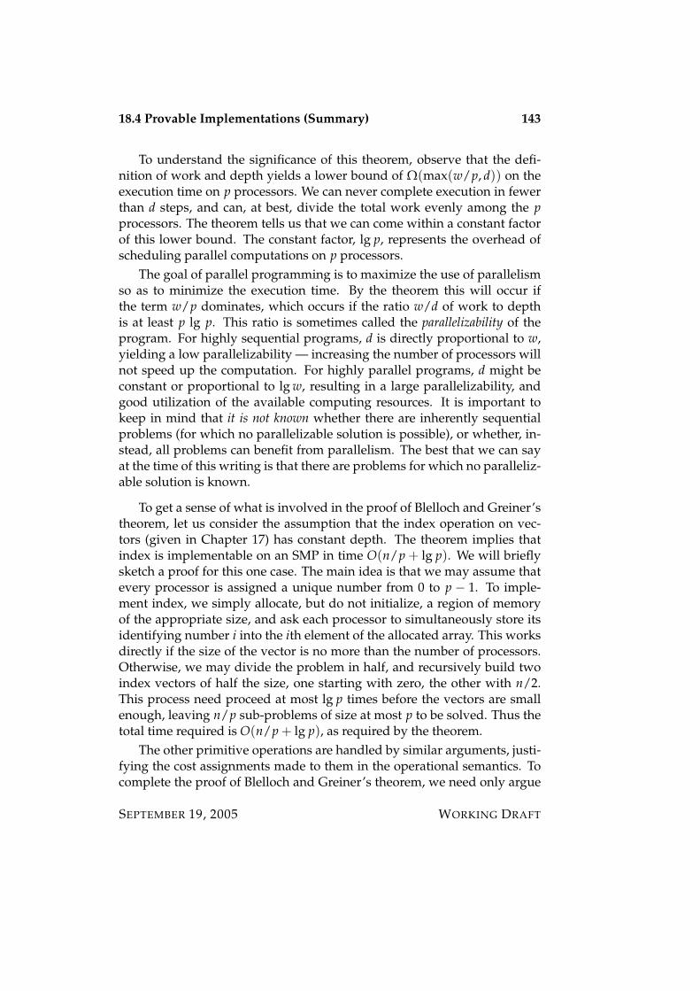
18.4 Provable Implementations (Summary) 143
To understand the significance of this theorem, observe that the defi-nition of work and depth yields a lower bound of Ω(max(w/p, d)) on theexecution time on p processors. We can never complete execution in fewerthan d steps, and can, at best, divide the total work evenly among the pprocessors. The theorem tells us that we can come within a constant factorof this lower bound. The constant factor, lg p, represents the overhead ofscheduling parallel computations on p processors.
The goal of parallel programming is to maximize the use of parallelismso as to minimize the execution time. By the theorem this will occur ifthe term w/p dominates, which occurs if the ratio w/d of work to depthis at least p lg p. This ratio is sometimes called the parallelizability of theprogram. For highly sequential programs, d is directly proportional to w,yielding a low parallelizability — increasing the number of processors willnot speed up the computation. For highly parallel programs, d might beconstant or proportional to lg w, resulting in a large parallelizability, andgood utilization of the available computing resources. It is important tokeep in mind that it is not known whether there are inherently sequentialproblems (for which no parallelizable solution is possible), or whether, in-stead, all problems can benefit from parallelism. The best that we can sayat the time of this writing is that there are problems for which no paralleliz-able solution is known.
To get a sense of what is involved in the proof of Blelloch and Greiner’stheorem, let us consider the assumption that the index operation on vec-tors (given in Chapter 17) has constant depth. The theorem implies thatindex is implementable on an SMP in time O(n/p + lg p). We will brieflysketch a proof for this one case. The main idea is that we may assume thatevery processor is assigned a unique number from 0 to p − 1. To imple-ment index, we simply allocate, but do not initialize, a region of memoryof the appropriate size, and ask each processor to simultaneously store itsidentifying number i into the ith element of the allocated array. This worksdirectly if the size of the vector is no more than the number of processors.Otherwise, we may divide the problem in half, and recursively build twoindex vectors of half the size, one starting with zero, the other with n/2.This process need proceed at most lg p times before the vectors are smallenough, leaving n/p sub-problems of size at most p to be solved. Thus thetotal time required is O(n/p + lg p), as required by the theorem.
The other primitive operations are handled by similar arguments, justi-fying the cost assignments made to them in the operational semantics. Tocomplete the proof of Blelloch and Greiner’s theorem, we need only argue
SEPTEMBER 19, 2005 WORKING DRAFT

144 18.4 Provable Implementations (Summary)
that the total work w can indeed be allocated to p processors with a costof only lg p for the overhead. This is a consequence of Brent’s Theorem,which states that a total workload w divided into d parallel steps may beimplemented on p processors in O(n/p + d lg p) time. The argument relieson certain assumptions about the SMP, including the ability to perform aparallel fetch-and-add operation in constant time.
WORKING DRAFT SEPTEMBER 19, 2005
Part VII
Data Structures andAbstraction
145

Chapter 19
Aggregate Data Structures
It is interesting to add to MinML support for programming with aggregatedata structures such as n-tuples, lists, and tree structures. We will decom-pose these familiar data structures into three types:
1. Product (or tuple) types. In general these are types whose values aren-tuples of values, with each component of a specified type. We willstudy two special cases that are sufficient to cover the general case:0-tuples (also known as the unit type) and 2-tuples (also known asordered pairs).
2. Sum (or variant or union) types. These are types whose values arevalues of one of n specified types, with an explicit “tag” indicatingwhich of the n choices is made.
3. Recursive types. These are “self-referential” types whose values mayhave as constituents values of the recursive type itself. Familiar ex-amples include lists and trees. A non-empty list consists of a value atthe head of the list together with another value of list type.
19.1 Products
The first-order abstract syntax associated with nullary and binary producttypes is given by the following grammar:
Types τ : : = unit | τ1*τ2Expressions e : : = () | check e1 is () in e2 | (e1,e2) |
split e1 as (x,y) in e2Values v : : = () | (v1,v2)
147
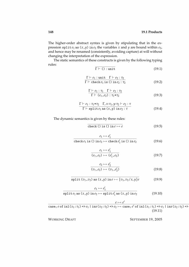
148 19.1 Products
The higher-order abstract syntax is given by stipulating that in the ex-pression split e1 as (x,y) in e2 the variables x and y are bound within e2,and hence may be renamed (consistently, avoiding capture) at will withoutchanging the interpretation of the expression.
The static semantics of these constructs is given by the following typingrules:
Γ ` () : unit (19.1)
Γ ` e1 : unit Γ ` e2 : τ2
Γ ` check e1 is () in e2 : τ2 (19.2)
Γ ` e1 : τ1 Γ ` e2 : τ2
Γ ` (e1,e2) : τ1*τ2 (19.3)
Γ ` e1 : τ1*τ2 Γ, x:τ1, y:τ2 ` e2 : τ
Γ ` split e1 as (x,y) in e2 : τ (19.4)
The dynamic semantics is given by these rules:
check () is () in e 7→ e (19.5)
e1 7→ e′1check e1 is () in e2 7→ check e′1 is () in e2 (19.6)
e1 7→ e′1(e1,e2) 7→ (e′1,e2) (19.7)
e2 7→ e′2(v1,e2) 7→ (v1,e′2) (19.8)
split (v1,v2) as (x,y) in e 7→ v1, v2/x, ye (19.9)
e1 7→ e′1split e1 as (x,y) in e2 7→ split e′1 as (x,y) in e2 (19.10)
e 7→ e′
caseτ e of inl(x1:τ1) => e1 | inr(x2:τ2) => e2 7→ caseτ e′ of inl(x1:τ1) => e1 | inr(x2:τ2) => e2(19.11)
WORKING DRAFT SEPTEMBER 19, 2005
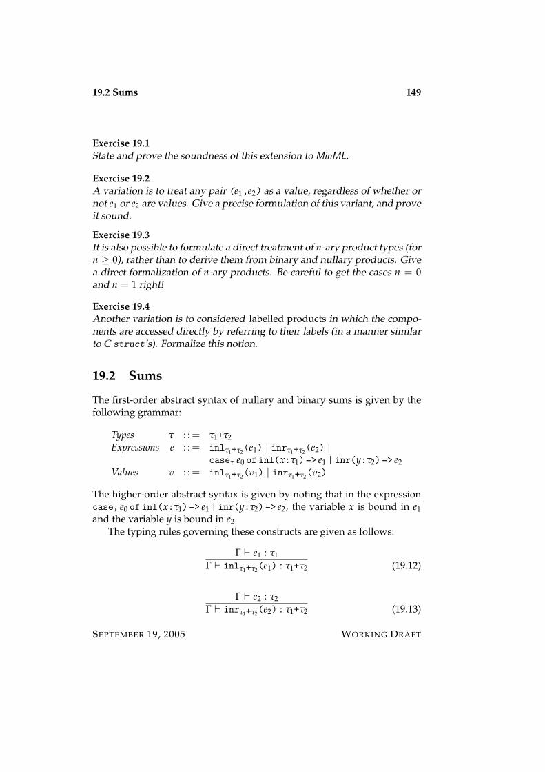
19.2 Sums 149
Exercise 19.1State and prove the soundness of this extension to MinML.
Exercise 19.2A variation is to treat any pair (e1,e2) as a value, regardless of whether ornot e1 or e2 are values. Give a precise formulation of this variant, and proveit sound.
Exercise 19.3It is also possible to formulate a direct treatment of n-ary product types (forn ≥ 0), rather than to derive them from binary and nullary products. Givea direct formalization of n-ary products. Be careful to get the cases n = 0and n = 1 right!
Exercise 19.4Another variation is to considered labelled products in which the compo-nents are accessed directly by referring to their labels (in a manner similarto C struct’s). Formalize this notion.
19.2 Sums
The first-order abstract syntax of nullary and binary sums is given by thefollowing grammar:
Types τ : : = τ1+τ2Expressions e : : = inlτ1+τ2(e1) | inrτ1+τ2(e2) |
caseτ e0 of inl(x:τ1) => e1 | inr(y:τ2) => e2Values v : : = inlτ1+τ2(v1) | inrτ1+τ2(v2)
The higher-order abstract syntax is given by noting that in the expressioncaseτ e0 of inl(x:τ1) => e1 | inr(y:τ2) => e2, the variable x is bound in e1and the variable y is bound in e2.
The typing rules governing these constructs are given as follows:
Γ ` e1 : τ1
Γ ` inlτ1+τ2(e1) : τ1+τ2 (19.12)
Γ ` e2 : τ2
Γ ` inrτ1+τ2(e2) : τ1+τ2 (19.13)
SEPTEMBER 19, 2005 WORKING DRAFT
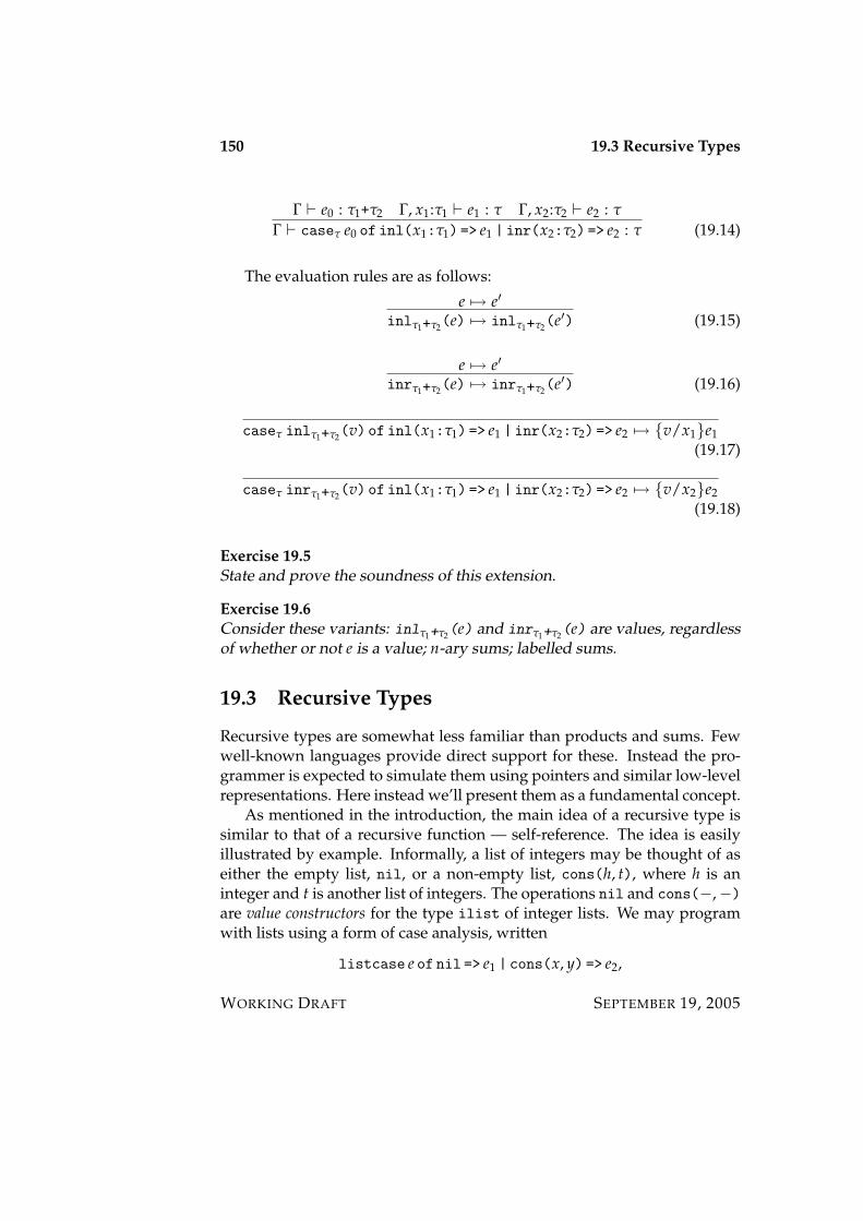
150 19.3 Recursive Types
Γ ` e0 : τ1+τ2 Γ, x1:τ1 ` e1 : τ Γ, x2:τ2 ` e2 : τ
Γ ` caseτ e0 of inl(x1:τ1) => e1 | inr(x2:τ2) => e2 : τ (19.14)
The evaluation rules are as follows:
e 7→ e′
inlτ1+τ2(e) 7→ inlτ1+τ2(e′) (19.15)
e 7→ e′
inrτ1+τ2(e) 7→ inrτ1+τ2(e′) (19.16)
caseτ inlτ1+τ2(v) of inl(x1:τ1) => e1 | inr(x2:τ2) => e2 7→ v/x1e1(19.17)
caseτ inrτ1+τ2(v) of inl(x1:τ1) => e1 | inr(x2:τ2) => e2 7→ v/x2e2(19.18)
Exercise 19.5State and prove the soundness of this extension.
Exercise 19.6Consider these variants: inlτ1+τ2(e) and inrτ1+τ2(e) are values, regardlessof whether or not e is a value; n-ary sums; labelled sums.
19.3 Recursive Types
Recursive types are somewhat less familiar than products and sums. Fewwell-known languages provide direct support for these. Instead the pro-grammer is expected to simulate them using pointers and similar low-levelrepresentations. Here instead we’ll present them as a fundamental concept.
As mentioned in the introduction, the main idea of a recursive type issimilar to that of a recursive function — self-reference. The idea is easilyillustrated by example. Informally, a list of integers may be thought of aseither the empty list, nil, or a non-empty list, cons(h, t), where h is aninteger and t is another list of integers. The operations nil and cons(−,−)are value constructors for the type ilist of integer lists. We may programwith lists using a form of case analysis, written
listcase e of nil => e1 | cons(x, y) => e2,
WORKING DRAFT SEPTEMBER 19, 2005
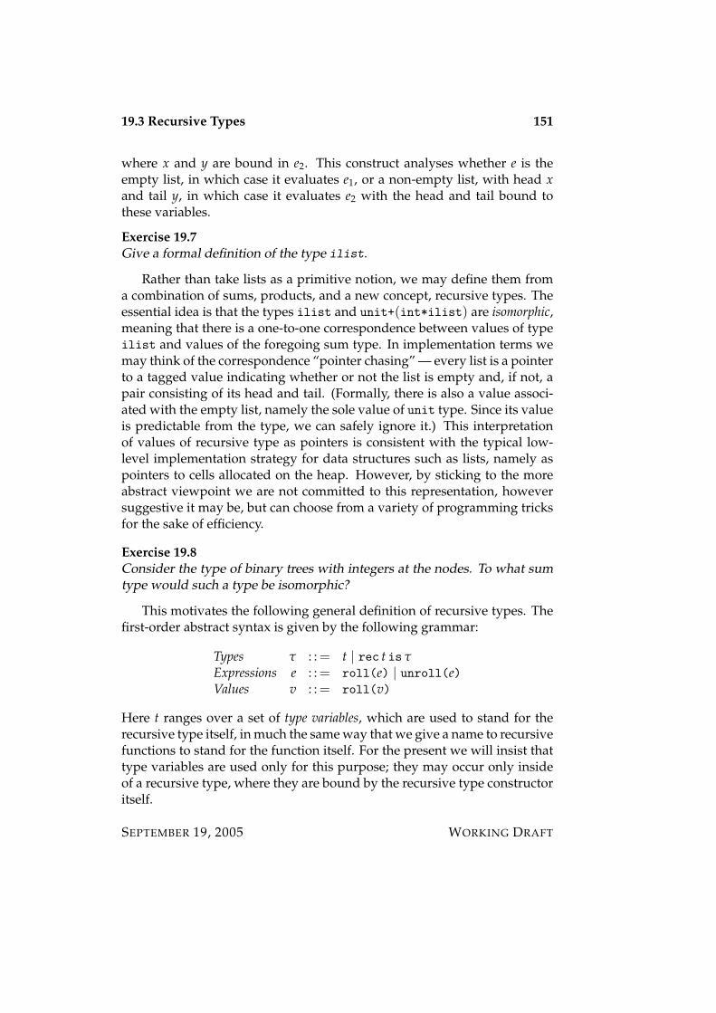
19.3 Recursive Types 151
where x and y are bound in e2. This construct analyses whether e is theempty list, in which case it evaluates e1, or a non-empty list, with head xand tail y, in which case it evaluates e2 with the head and tail bound tothese variables.
Exercise 19.7Give a formal definition of the type ilist.
Rather than take lists as a primitive notion, we may define them froma combination of sums, products, and a new concept, recursive types. Theessential idea is that the types ilist and unit+(int*ilist) are isomorphic,meaning that there is a one-to-one correspondence between values of typeilist and values of the foregoing sum type. In implementation terms wemay think of the correspondence “pointer chasing” — every list is a pointerto a tagged value indicating whether or not the list is empty and, if not, apair consisting of its head and tail. (Formally, there is also a value associ-ated with the empty list, namely the sole value of unit type. Since its valueis predictable from the type, we can safely ignore it.) This interpretationof values of recursive type as pointers is consistent with the typical low-level implementation strategy for data structures such as lists, namely aspointers to cells allocated on the heap. However, by sticking to the moreabstract viewpoint we are not committed to this representation, howeversuggestive it may be, but can choose from a variety of programming tricksfor the sake of efficiency.
Exercise 19.8Consider the type of binary trees with integers at the nodes. To what sumtype would such a type be isomorphic?
This motivates the following general definition of recursive types. Thefirst-order abstract syntax is given by the following grammar:
Types τ : : = t | rec t is τExpressions e : : = roll(e) | unroll(e)Values v : : = roll(v)
Here t ranges over a set of type variables, which are used to stand for therecursive type itself, in much the same way that we give a name to recursivefunctions to stand for the function itself. For the present we will insist thattype variables are used only for this purpose; they may occur only insideof a recursive type, where they are bound by the recursive type constructoritself.
SEPTEMBER 19, 2005 WORKING DRAFT
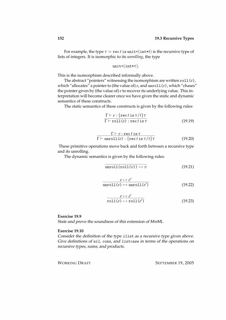
152 19.3 Recursive Types
For example, the type τ = rec t is unit+(int*t) is the recursive type oflists of integers. It is isomorphic to its unrolling, the type
unit+(int*τ).
This is the isomorphism described informally above.The abstract “pointers” witnessing the isomorphism are written roll(e),
which “allocates” a pointer to (the value of) e, and unroll(e), which “chases”the pointer given by (the value of) e to recover its underlying value. This in-terpretation will become clearer once we have given the static and dynamicsemantics of these constructs.
The static semantics of these constructs is given by the following rules:
Γ ` e : rec t is τ/tτΓ ` roll(e) : rec t is τ (19.19)
Γ ` e : rec t is τΓ ` unroll(e) : rec t is τ/tτ (19.20)
These primitive operations move back and forth between a recursive typeand its unrolling.
The dynamic semantics is given by the following rules:
unroll(roll(v)) 7→ v (19.21)
e 7→ e′
unroll(e) 7→ unroll(e′) (19.22)
e 7→ e′
roll(e) 7→ roll(e′) (19.23)
Exercise 19.9State and prove the soundness of this extension of MinML.
Exercise 19.10Consider the definition of the type ilist as a recursive type given above.Give definitions of nil, cons, and listcase in terms of the operations onrecursive types, sums, and products.
WORKING DRAFT SEPTEMBER 19, 2005
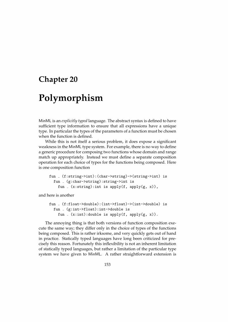
Chapter 20
Polymorphism
MinML is an explicitly typed language. The abstract syntax is defined to havesufficient type information to ensure that all expressions have a uniquetype. In particular the types of the parameters of a function must be chosenwhen the function is defined.
While this is not itself a serious problem, it does expose a significantweakness in the MinML type system. For example, there is no way to definea generic procedure for composing two functions whose domain and rangematch up appropriately. Instead we must define a separate compositionoperation for each choice of types for the functions being composed. Hereis one composition function
fun (f:string->int):(char->string)->(string->int) isfun (g:char->string):string->int isfun (x:string):int is apply(f, apply(g, x)),
and here is another
fun (f:float->double):(int->float)->(int->double) isfun (g:int->float):int->double isfun (x:int):double is apply(f, apply(g, x)).
The annoying thing is that both versions of function composition exe-cute the same way; they differ only in the choice of types of the functionsbeing composed. This is rather irksome, and very quickly gets out of handin practice. Statically typed languages have long been criticized for pre-cisely this reason. Fortunately this inflexibility is not an inherent limitationof statically typed languages, but rather a limitation of the particular typesystem we have given to MinML. A rather straightforward extension is
153

154 20.1 A Polymorphic Language
sufficient to provide the kind of flexibility that is essential for a practicallanguage. This extension is called polymorphism.
While ML has had such a type system from its inception (circa 1978),few other languages have followed suit. Notably the Java language suffersfrom this limitation (but the difficulty is mitigated somewhat in the pres-ence of subtyping). Plans are in the works, however, for adding polymor-phism (called generics) to the Java language. A compiler for this extension,called Generic Java, is already available.
20.1 A Polymorphic Language
Polymorphic MinML, or PolyMinML, is an extension of MinML with the abil-ity to define polymorphic functions. Informally, a polymorphic function is afunction that takes a type as argument and yields a value as result. The typeparameter to a polymorphic function represents an unknown, or generic,type, which can be instantiated by applying the function to a specific type.The types of polymorphic functions are called polymorphic types, or poly-types.
A significant design decision is whether to regard polymorphic typesas “first-class” types, or whether they are, instead, “second-class” citizens.Polymorphic functions in ML are second-class — they cannot be passed asarguments, returned as results, or stored in data structures. The only thingwe may do with polymorphic values is to bind them to identifiers with aval or fun binding. Uses of such identifiers are automatically instantiatedby an implicit polymorphic instantiation. The alternative is to treat poly-morphic functions as first-class values, which can be used like any othervalue in the language. Here there are no restrictions on how they can beused, but you should be warned that doing so precludes using type infer-ence to perform polymorphic abstraction and instantiation automatically.
We’ll set things up for second-class polymorphism by explicitly distin-guishing polymorphic types from monomorphic types. The first-class casecan then be recovered by simply conflating polytypes and monotypes.
WORKING DRAFT SEPTEMBER 19, 2005

20.1 A Polymorphic Language 155
Abstract Syntax
The abstract syntax of PolyMinML is defined by the following extension tothe MinML grammar:
Polytypes σ : : = τ | ∀t(σ)Monotypes τ : : = . . . | tExpressions e : : = . . . | Fun t in e | inst(e,τ)Values v : : = . . . | Fun t in e
The variable t ranges over a set of type variables, which are written ML-style’a, ’b, and so on in examples. In the polytype ∀t(σ) the type variable tis bound in σ; we do not distinguish between polytypes that differ onlyin the names of bound variables. Since the quantifier can occur only atthe outermost level, in ML it is left implicit. An expression of the formFun t in e is a polymorphic function with parameter t and body e. The variablet is bound within e. An expression of the form inst(e,τ) is a polymorphicinstantiation of the polymorphic function e at monotype τ. Notice that wemay only instantiate polymorphic functions with monotypes. In exampleswe write f[τ] for polymorphic instantiation, rather than the more verboseinst( f,τ).
We write FTV(τ) (respectively, FTV(σ), FTV(e)) for the set of free typevariables occurring in τ (respectively, σ, e). Capture-avoiding substitu-tion of a monotype τ for free occurrences of a type variable t in a poly-type σ (resp., monotype τ′, expression e) is written τ/tσ (resp., τ/tτ′,τ/te).
Static Semantics
The static semantics of PolyMinML is a straightforward extension to that ofMinML. One significant change, however, is that we must now keep trackof the scopes of type variables, as well as ordinary variables. In the staticsemantics of MinML a typing judgement had the form Γ ` e : τ, whereΓ is a context assigning types to ordinary variables. Only those variablesin dom Γ may legally occur in e. For PolyMinML we must introduce anadditional context, ∆, which is a set of type variables, those that may legallyoccur in the types and expression of the judgement.
The static semantics consists of rules for deriving the following twojudgements:
∆ ` σ ok σ is a well-formed type in ∆Γ `∆ e : σ e is a well-formed expression of type σ in Γ and ∆
SEPTEMBER 19, 2005 WORKING DRAFT

156 20.1 A Polymorphic Language
The rules for validity of types are as follows:
t ∈ ∆∆ ` t ok (20.1)
∆ ` int ok (20.2)
∆ ` bool ok (20.3)
∆ ` τ1 ok ∆ ` τ2 ok
∆ ` τ1→τ2 ok (20.4)
∆ ∪ t ` σ ok t /∈ ∆∆ ` ∀t(σ) ok (20.5)
The auxiliary judgement ∆ ` Γ is defined by the following rule:
∆ ` Γ(x) ok (∀x ∈ dom(Γ))∆ ` Γ ok . (20.6)
The rules for deriving typing judgements Γ `∆ e : σ are as follows. Weassume that ∆ ` Γ ok, ∆ ` σ ok, FV(e) ⊆ dom(Γ), and FTV(e) ⊆ ∆. Wegive only the rules specific to PolyMinML; the remaining rules are those ofMinML, augmented with a set ∆ of type variables.
Γ `∆∪ t e : σ t /∈ ∆
Γ `∆ Fun t in e : ∀t(σ) (20.7)
Γ `∆ e : ∀t(σ) ∆ ` τ ok
Γ `∆ inst(e,τ) : τ/tσ (20.8)
For example, here is the polymorphic composition function in PolyMinML:
Fun t inFun u inFun v infun (f:u->v):(t->u)->(t->v) isfun (g:t->u):t->v isfun (x:t):v is apply(f, apply(g, x))
WORKING DRAFT SEPTEMBER 19, 2005
20.1 A Polymorphic Language 157
It is easy to check that it has type
∀t(∀u(∀v((u→v)→(t→u)→(t→v)))).
We will need the following technical lemma stating that typing is pre-served under instantiation:
Lemma 20.1 (Instantiation)If Γ `∆∪ t e : σ, where t /∈ ∆, and ∆ ` τ ok, then τ/tΓ `∆ τ/te :τ/tσ.
The proof is by induction on typing, and involves no new ideas beyondwhat we have already seen.
We will also have need of the following canonical forms lemma:
Lemma 20.2 (Canonical Forms)If v : ∀t(σ), then v = Fun t in e for some t and e such that ∅ ` t e : σ.
This is proved by a straightforward analysis of the typing rules.
Dynamic Semantics
The dynamic semantics of PolyMinML is a simple extension of that of MinML.We need only add the following two SOS rules:
inst(Fun t in e,τ) 7→ τ/te (20.9)
e 7→ e′
inst(e,τ) 7→ inst(e′,τ) (20.10)
It is then a simple matter to prove safety for this language.
Theorem 20.3 (Preservation)If e : σ and e 7→ e′, then e′ : σ.
The proof is by induction on evaluation.
Theorem 20.4 (Progress)If e : σ, then either e is a value or there exists e′ such that e 7→ e′.
As before, this is proved by induction on typing.
SEPTEMBER 19, 2005 WORKING DRAFT
158 20.1 A Polymorphic Language
First-Class Polymorphism
The syntax given above describes an ML-like treatment of polymorphism,albeit one in which polymorphic abstraction and instantiation is explicit,rather than implicit, as it is in ML. To obtain the first-class variant of PolyMinML,we simply ignore the distinction between poly- and mono-types, regardingthem all as simply types. Everything else remains unchanged, includingthe proofs of progress and preservation.
With first-class polymorphism we may consider types such as
∀t(t→t)→∀t(t→t),
which cannot be expressed in the ML-like fragment. This is the type offunctions that accept a polymorphic function as argument and yield a poly-morphic function (of the same type) as result. If f has the above type,then f(Fun t in fun (x:t):t is x) is well-formed. However, the applica-tion f(fun (x:int):int is+(x, 1)) is ill-formed, because the successorfunction does not have type ∀t(t→t). The requirement that the argumentbe polymorphic is a significant restriction on how f may be used!
Contrast this with the following type (which does lie within the ML-likefragment):
∀t((t→t)→(t→t)).
This is the type of polymorphic functions that, for each type t, accept afunction on t and yield another function on t. If g has this type, the expres-sion inst(g,int)(succ) is well-formed, since we first instantiate g at int,then apply it to the successor function.
The situation gets more interesting in the presence of data structuressuch as lists and reference cells. It is a worthwhile exercise to consider thedifference between the types ∀t(σ) list and ∀t(σ list) for various choicesof σ. Note once again that the former type cannot be expressed in ML,whereas the latter can.
Recall the following counterexample to type soundness for the earlyversion of ML without the so-called value restriction:
letval r : (’a -> ’a) ref = ref (fn x:’a => x)
inr := (fn x:int => x+1) ; (!r)(true)
end
WORKING DRAFT SEPTEMBER 19, 2005
20.1 A Polymorphic Language 159
A simple check of the polymorphic typing rules reveals that this is a well-formed expression, provided that the value restriction is suspended. Ofcourse, it “gets stuck” during evaluation by attempting to add 1 to true.
Using the framework of explicit polymorphism, I will argue that thesuperficial plausibility of this example (which led to the unsoundness inthe language) stems from a failure to distinguish between these two types:
1. The type ∀t(t→t ref) of polymorphic functions yielding referencecells containing a function from a type to itself.
2. The type ∀t(t→t) ref of reference cells containing polymorphic func-tions yielding a function from a type to itself.
(Notice the similarity to the distinctions discussed above.) For this exampleto be well-formed, we rely on an inconsistent reading of the example. Atthe point of the val binding we are treating r as a value of the latter type,namely a reference cell containing a polymorphic function. But in the bodyof the let we are treating it as a value of the former type, a polymorphicfunction yielding a reference cell. We cannot have it both ways at once!
To sort out the error let us make the polymorphic instantiation and ab-straction explicit. Here’s one rendering:
letval r : All ’a ((’a -> ’a) ref) =Fun ’a in ref (fn x:’a => x) end
inr[int] := (fn x:int => x+1) ; (!(r[bool]))(true)
end
Notice that we have made the polymorphic abstraction explicit, and in-serted corresponding polymorphic instantiations. This example is type cor-rect, and hence (by the proof of safety above) sound. But notice that it al-locates two reference cells, not one! Recall that polymporphic functions arevalues, and the binding of r is just such a value. Each of the two instancesof r executes the body of this function separately, each time allocating anew reference cell. Hence the unsoundness goes away!
Here’s another rendering that is, in fact, ill-typed (and should be, sinceit “gets stuck”!).
SEPTEMBER 19, 2005 WORKING DRAFT
160 20.2 ML-style Type Inference
letval r : (All ’a (’a -> ’a)) ref =ref (Fun ’a in fn x:’a => x end)
inr := (fn x:int => x+1) ; (!r)[bool](true)
end
The assignment to r is ill-typed because the successor is not sufficientlypolymorphic. The retrieval and subsequent instantiation and application istype-correct, however. If we change the program to
letval r : (All ’a (’a -> ’a)) ref =ref (Fun ’a in fn x:’a => x end)
inr := (Fun ’a in fn x:’a => x end) ; (!r)[bool](true)
end
then the expression is well-typed, and behaves sanely, precisely because wehave assigned to r a sufficiently polymorphic function.
20.2 ML-style Type Inference
ML-style type inference may be viewed as a translation from the implicitlytyped syntax of ML to the explicitly-typed syntax of PolyMinML. Specifi-cally, the type inference mechanism performs the following tasks:
• Attaching type labels to function arguments and results.
• Inserting polymorphic abstractions for declarations of polymorphictype.
• Inserting polymorphic instantiations whenever a polymorphic de-clared variable is used.
Thus in ML we may write
val I : ’a -> ’a = fn x => xval n : int = I(I)(3)
This stands for the PolyMinML declarations1
1We’ve not equipped PolyMinML with a declaration construct, but you can see from theexample how this might be done.
WORKING DRAFT SEPTEMBER 19, 2005

20.3 Parametricity 161
val I : ∀t(t→t) = Fun t in fun (x:t):t is xval n : int = inst(I,int→int)(inst(I,int))(3)
Here we apply the polymorphic identity function to itself, then apply theresult to 3. The identity function is explicitly abstracted on the type of itsargument and result, and its domain and range types are made explicit onthe function itself. The two occurrences of I in the ML code are replaced byinstantiations of I in the PolyMinML code, first at type int→int, the secondat type int.
With this in mind we can now explain the “value restriction” on poly-morphism in ML. Referring to the example of the previous section, thetype inference mechanism of ML generates the first rendering of the ex-ample give above in which the type of the reference cell is ∀t((t→t) ref).As we’ve seen, when viewed in this way, the example is not problematic,provided that polymorphic abstractions are seen as values. For in this casethe two instances of r generate two distinct reference cells, and no difficul-ties arise. Unfortunately, ML does not treat polymorphic abstractions asvalues! Only one reference cell is allocated, which, in the absence of thevalue restriction, would lead to unsoundness.
Why does the value restriction save the day? In the case that the poly-morphic expression is not a value (in the ML sense) the polymorphic ab-straction that is inserted by the type inference mechanism changes a non-value into a value! This changes the semantics of the expression (as we’veseen, from allocating one cell, to allocating two different cells), which vio-lates the semantics of ML itself.2 However, if we limit ourselves to valuesin the first place, then the polymorphic abstraction is only ever wrappedaround a value, and no change of semantics occurs. Therefore3, the inser-tion of polymorphic abstraction doesn’t change the semantics, and every-thing is safe. The example above involving reference cells is ruled out, be-cause the expression ref (fn x => x) is not a value, but such is the natureof the value restriction.
20.3 Parametricity
Our original motivation for introducing polymorphism was to enable moreprograms to be written — those that are “generic” in one or more types,such as the composition function give above. The idea is that if the behavior
2One could argue that the ML semantics is incorrect, which leads to a different language.3This would need to be proved, of course.
SEPTEMBER 19, 2005 WORKING DRAFT
162 20.3 Parametricity
of a function does not depend on a choice of types, then it is useful to be ableto define such “type oblivious” functions in the language. Once we havesuch a mechanism in hand, it can also be used to ensure that a particularpiece of code can not depend on a choice of types by insisting that it bepolymorphic in those types. In this sense polymorphism may be used toimpose restrictions on a program, as well as to allow more programs to bewritten.
The restrictions imposed by requiring a program to be polymorphic un-derlie the often-observed experience when programming in ML that if thetypes are correct, then the program is correct. Roughly speaking, since theML type system is polymorphic, if a function type checks with a polymor-phic type, then the strictures of polymorphism vastly cut down the set ofwell-typed programs with that type. Since the intended program is onethese (by the hypothesis that its type is “right”), you’re much more likelyto have written it if the set of possibilities is smaller.
The technical foundation for these remarks is called parametricity. Thegoal of this section is to give an account of parametricity for PolyMinML.To keep the technical details under control, we will restrict attention to theML-like (prenex) fragment of PolyMinML. It is possibly to generalize tofirst-class polymorphism, but at the expense of considerable technical com-plexity. Nevertheless we will find it necessary to gloss over some technicaldetails, but wherever a “pedagogic fiction” is required, I will point it out.To start with, it should be stressed that the following does not apply to lan-guages with mutable references!
20.3.1 Informal Discussion
We will begin with an informal discussion of parametricity based on a “seatof the pants” understanding of the set of well-formed programs of a type.
Suppose that a function value f has the type ∀t(t→t). What functioncould it be?
1. It could diverge when instantiated — f [τ] goes into an infinite loop.Since f is polymorphic, its behavior cannot depend on the choice ofτ, so in fact f [τ′] diverges for all τ′ if it diverges for τ.
2. It could converge when instantiated at τ to a function g of type τ→τthat loops when applied to an argument v of type τ — i.e., g(v) runsforever. Since f is polymorphic, g must diverge on every argument vof type τ if it diverges on some argument of type τ.
WORKING DRAFT SEPTEMBER 19, 2005

20.3 Parametricity 163
3. It could converge when instantiated at τ to a function g of type τ→τthat, when applied to a value v of type τ returns a value v′ of typeτ. Since f is polymorphic, g cannot depend on the choice of v, so v′
must in fact be v.
Let us call cases (1) and (2) uninteresting. The foregoing discussion sug-gests that the only interesting function f of type ∀t(t→t) is the polymorphicidentity function.
Suppose that f is an interesting function of type ∀t(t). What functioncould it be? A moment’s thought reveals that it cannot be interesting! Thatis, every function f of this type must diverge when instantiated, and henceis uninteresting. In other words, there are no interesting values of this type— it is essentially an “empty” type.
For a final example, suppose that f is an interesting function of type∀t(t list→t list). What function could it be?
1. The identity function that simply returns its argument.
2. The constantly-nil function that always returns the empty list.
3. A function that drops some elements from the list according to a pre-determined (data-independent) algorithm — e.g., always drops thefirst three elements of its argument.
4. A permutation function that reorganizes the elements of its argu-ment.
The characteristic that these functions have in common is that their behav-ior is entirely determined by the spine of the list, and is independent ofthe elements of the list. For example, f cannot be the function that dropsall “even” elements of the list — the elements might not be numbers! Thepoint is that the type of f is polymorphic in the element type, but revealsthat the argument is a list of unspecified elements. Therefore it can onlydepend on the “list-ness” of its argument, and never on its contents.
In general if a polymorphic function behaves the same at every typeinstance, we say that it is parametric in that type. In PolyMinML all polymor-phic functions are parametric. In Standard ML most functions are, exceptthose that involve equality types. The equality function is not parametric be-cause the equality test depends on the type instance — testing equality ofintegers is different than testing equality of floating point numbers, and wecannot test equality of functions. Such “pseudo-polymorphic” operationsare said to be ad hoc, to contrast them from parametric.
SEPTEMBER 19, 2005 WORKING DRAFT
164 20.3 Parametricity
How can parametricity be exploited? As we will see later, parametric-ity is the foundation for data abstraction in a programming language. Toget a sense of the relationship, let us consider a classical example of ex-ploiting parametricity, the polymorphic Church numerals. Let N be the type∀t(t→(t→t)→t). What are the interesting functions of the type N? Givenany type τ, and values z : τ and s : τ→τ, the expression
f [τ](z)(s)
must yield a value of type τ. Moreover, it must behave uniformly withrespect to the choice of τ. What values could it yield? The only way tobuild a value of type τ is by using the element z and the function s passedto it. A moment’s thought reveals that the application must amount to then-fold composition
s(s(. . . s(z) . . .)).
That is, the elements of N are in 1-to-1 correspondence with the naturalnumbers.
Let us write n for the polymorphic function of type N representing thenatural number n, namely the function
Fun t infn z:t in
fn s:t->t ins(s(... s)...))
endend
end
where there are n occurrences of s in the expression. Observe that if weinstantiate n at the built-in type int and apply the result to 0 and succ,it evaluates to the number n. In general we may think of performing an“experiment” on a value of type N by instantiating it at a type whose valueswill constitute the observations, the applying it to operations z and s forperforming the experiment, and observing the result.
Using this we can calculate with Church numerals. Let us consider howto define the addition function on N. Given m and n of type N, we wishto compute their sum m + n, also of type N. That is, the addition functionmust look as follows:
WORKING DRAFT SEPTEMBER 19, 2005
20.3 Parametricity 165
fn m:N infn n:N in
Fun t infn z:t in
fn s:t->t in...
endend
endend
end
The question is: how to fill in the missing code? Think in terms of ex-periments. Given m and n of type N, we are to yield a value that when“probed” by supplying a type t, an element z of that type, and a function son that type, must yield the (m + n)-fold composition of s with z. One wayto do this is to “run” m on t, z, and s, yielding the m-fold composition of swith z, then “running” n on this value and s again to obtain the n-fold com-position of s with the n-fold composition of s with z — the desired answer.Here’s the code:
fn m:N infn n:N in
Fun t infn z:t in
fn s:t->t inn[t](m[t](z)(s))(s)
endend
endend
end
To see that it works, instantiate the result at τ, apply it to z and s, andobserve the result.
20.3.2 Relational Parametricity
In this section we give a more precise formulation of parametricity. Themain idea is that polymorphism implies that certain equations between ex-pressions must hold. For example, if f : ∀t(t→t), then f must be equal to
SEPTEMBER 19, 2005 WORKING DRAFT
166 20.3 Parametricity
the identity function, and if f : N, then f must be equal to some Churchnumeral n. To make the informal idea of parametricity precise, we mustclarify what we mean by equality of expressions.
The main idea is to define equality in terms of “experiments” that wecarry out on expressions to “test” whether they are equal. The valid experi-ments on an expression are determined solely by its type. In general we saythat two closed expressions of a type τ are equal iff either they both diverge,or they both converge to equal values of that type. Equality of closed val-ues is then defined based on their type. For integers and booleans, equalityis straightforward: two values are equal iff they are identical. The intu-ition here is that equality of numbers and booleans is directly observable.Since functions are “infinite” objects (when thought of in terms of their in-put/output behavior), we define equality in terms of their behavior whenapplied. Specifically, two functions f and g of type τ1→τ2 are equal iffwhenever they are applied to equal arguments of type τ1, they yield equalresults of type τ2.
More formally, we make the following definitions. First, we defineequality of closed expressions of type τ as follows:
e ∼=exp e′ : τ iff e 7→∗ v⇔ e′ 7→∗ v′ andv ∼=val v′ : τ.
Notice that if e and e′ both diverge, then they are equal expressions in thissense. For closed values, we define equality by induction on the structureof monotypes:
v ∼=val v′ : bool iff v = v′ = true or v = v′ = falsev ∼=val v′ : int iff v = v′ = n for some n ≥ 0
v ∼=val v′ : τ1→τ2 iff v1∼=val v′1 : τ1 implies v(v1) ∼=exp v′(v′1) : τ2
The following lemma states two important properties of this notion ofequality.
Lemma 20.51. Expression and value equivalence are reflexive, symmetric, and tran-
sitive.
2. Expression equivalence is a congruence: we may replace any sub-expression of an expression e by an equivalent sub-expression to ob-tain an equivalent expression.
So far we’ve considered only equality of closed expressions of monomor-phic type. The definition is made so that it readily generalizes to the poly-morphic case. The idea is that when we quantify over a type, we are not
WORKING DRAFT SEPTEMBER 19, 2005
20.3 Parametricity 167
able to say a priori what we mean by equality at that type, precisely be-cause it is “unknown”. Therefore we also quantify over all possible notionsof equality to cover all possible interpretations of that type. Let us writeR : τ ↔ τ′ to indicate that R is a binary relation between values of type τand τ′.
Here is the definition of equality of polymorphic values:
v ∼=val v′ : ∀t(σ) iff for all τ and τ′, and all R : τ ↔ τ′, v [τ] ∼=exp v′ [τ′] : σ
where we take equality at the type variable t to be the relation R (i.e., v ∼=valv′ : t iff v R v′).
There is one important proviso: when quantifying over relations, wemust restrict attention to what are called admissible relations, a sub-classof relations that, in a suitable sense, respects computation. Most naturalchoices of relation are admissible, but it is possible to contrive examplesthat are not. The rough-and-ready rule is this: a relation is admissible iffit is closed under “partial computation”. Evaluation of an expression e toa value proceeds through a series of intermediate expressions e 7→ e1 7→e2 7→ · · · en. The expressions ei may be thought of as “partial computations”of e, stopping points along the way to the value of e. If a relation relatescorresponding partial computations of e and e′, then, to be admissible, itmust also relate e and e′ — it cannot relate all partial computations, andthen refuse to relate the complete expressions. We will not develop thisidea any further, since to do so would require the formalization of partialcomputation. I hope that this informal discussion suffices to give the idea.
The following is Reynolds’ Parametricity Theorem:
Theorem 20.6 (Parametricity)If e : σ is a closed expression, then e ∼=exp e : σ.
This may seem obvious, until you consider that the notion of equality be-tween expressions of polymorphic type is very strong, requiring equiva-lence under all possible relational interpretations of the quantified type.
Using the Parametricity Theorem we may prove a result we stated in-formally above.
Theorem 20.7If f : ∀t(t→t) is an interesting value, then f ∼=val id : ∀t(t→t), where id isthe polymorphic identity function.
Proof: Suppose that τ and τ′ are monotypes, and that R : τ ↔ τ′. We wishto show that
f [τ] ∼=exp id [τ′] : t→t,
SEPTEMBER 19, 2005 WORKING DRAFT
168 20.3 Parametricity
where equality at type t is taken to be the relation R.Since f (and id) are interesting, there exists values fτ and idτ′ such that
f [τ] 7→∗ fτ
andid [τ′] 7→∗ idτ′ .
We wish to show thatfτ∼=val idτ′ : t→t.
Suppose that v1∼=val v′1 : t, which is to say v1 R v′1 since equality at type
t is taken to be the relation R. We are to show that
fτ(v1) ∼=exp idτ′(v′1) : t
By the assumption that f is interesting (and the fact that id is interesting),there exists values v2 and v′2 such that
fτ(v1) 7→∗ v2
andidτ′(v′1) 7→∗ v′2.
By the definition of id, it follows that v′2 = v′1 (it’s the identity function!).We must show that v2 R v′1 to complete the proof.
Now define the relation R′ : τ ↔ τ to be the set (v, v) | v R v′1 .Since f : ∀t(t→t), we have by the Parametricity Theorem that f ∼=val f :∀t(t→t), where equality at type t is taken to be the relation R′. Since v1 R v′1,we have by definition v1 R′ v1. Using the definition of equality of polymor-phic type, it follows that
fτ(v1) ∼=exp idτ′(v1) : t.
Hence v2 R v′1, as required.
You might reasonably wonder, at this point, what the relationship f ∼=valid : ∀t(t→t) has to do with f ’s execution behavior. It is a general fact, whichwe will not attempt to prove, that equivalence as we’ve defined it yields re-sults about execution behavior. For example, if f : ∀t(t→t), we can showthat for every τ and every v : τ, f [τ](v) evaluates to v. By the precedingtheorem f ∼=val id : ∀t(t→t). Suppose that τ is some monotype and v : τ issome closed value. Define the relation R : τ ↔ τ by
v1 R v2 iff v1 = v2 = v.
WORKING DRAFT SEPTEMBER 19, 2005

20.3 Parametricity 169
Then we have by the definition of equality for polymorphic values
f [τ](v) ∼=exp id [τ](v) : t,
where equality at t is taken to be the relation R. Since the right-hand sideterminates, so must the left-hand side, and both must yield values relatedby R, which is to say that both sides must evaluate to v.
SEPTEMBER 19, 2005 WORKING DRAFT

170 20.3 Parametricity
WORKING DRAFT SEPTEMBER 19, 2005
Chapter 21
Data Abstraction
Data abstraction is perhaps the most fundamental technique for structur-ing programs to ensure their robustness over time and to facilitate teamdevelopment. The fundamental idea of data abstraction is the separationof the client from the implementor of the abstraction by an interface. Theinterface is a form of “contract” between the client and implementor. Itspecifies the operations that may be performed on values of the abstracttype by the client and, at the same time, imposes the obligation on the im-plementor to provide these operations with the specified functionality. Bylimiting the client’s view of the abstract type to a specified set of operations,the interface protects the client from depending on the details of the imple-mentation of the abstraction, most especially its representation in terms ofwell-known constructs of the programming language. Doing so ensuresthat the implementor is free to change the representation (and, correspond-ingly, the implementation of the operations) of the abstract type withoutaffecting the behavior of a client of the abstraction.
Our intention is to develop a rigorous account of data abstraction in anextension of PolyMinML with existential types. Existential types provide thefundamental linguistic mechanisms for defining interfaces, implementingthem, and using the implementation in client code. Using this extensionof PolyMinML we will then develop a formal treatment of representationindependence based on Reynolds’s Parametricity Theorem for PolyMinML.The representation independence theorem will then serve as the basis forproving the correctness of abstract type implementations using bisimula-tion relations.
171
172 21.1 Existential Types
21.1 Existential Types
21.1.1 Abstract Syntax
The syntax of PolyMinML is extended with the following constructs:
Polytypes σ : : = . . .| ∃t(σ)
Expressions e : : = . . .| pack τ with e as σ| open e1 as t with x:σ in e2
Values v : : = . . .| pack τ with v as σ
The polytype ∃t(σ) is called an existential type. An existential type is the in-terface of an abstract type. An implementation of the existential type ∃t(σ) isa package value of the form pack τ with v as ∃t(σ) consisting of a monotypeτ together with a value v of type τ/tσ. The monotype τ is the represen-tation type of the implementation; the value v is the implementation of theoperations of the abstract type. A client makes use of an implementationby opening it within a scope, written open ei as t with x:σ in ec, where ei isan implementation of the interface ∃t(σ), and ec is the client code definedin terms of an unknown type t (standing for the representation type) andan unknown value x of type σ (standing for the unknown operations).
In an existential type ∃t(σ) the type variable t is bound in σ, and may berenamed at will to satisfy uniqueness requirements. In an expression of theform open ei as t with x:σ in ec the type variable t and the ordinary variablex are bound in ec, and may also be renamed at will to satisfy non-occurrencerequirements. As we will see below, renaming of bound variables is crucialfor ensuring that an abstract type is “new” in the sense of being distinctfrom any other type whenever it is opened for use in a scope. This is some-times called generativity of abstract types, since each occurrence of open“generates” a “new” type for use within the body of the client. In real-ity this informal notion of generativity comes down to renaming of boundvariables to ensure their uniqueness in a context.
21.1.2 Correspondence With ML
To fix ideas, it is worthwhile to draw analogies between the present formal-ism and (some aspects of) the Standard ML module system. We have thefollowing correspondences:
WORKING DRAFT SEPTEMBER 19, 2005

21.1 Existential Types 173
PolyMinML + Existentials Standard MLExistential type SignaturePackage Structure, with opaque ascriptionOpening a package open declaration
Here is an example of these correspondences in action. In the sequel wewill use ML-like notation with the understanding that it is to be interpretedin PolyMinML in the following fashion.
Here is an ML signature for a persistent representation of queues:
signature QUEUE =sigtype queueval empty : queueval insert : int * queue -> queueval remove : queue -> int * queue
end
This signature is deliberately stripped down to simplify the development.In particular we leave undefined the meaning of remove on an empty queue.
The corresponding existential type is σq : = ∃q(τq), where
τq : = q*((int*q)→q)*(q→(int*q))
That is, the operations of the abstraction consist of a three-tuple of values,one for the empty queue, one for the insert function, and one for the removefunction.
Here is a straightforward implementation of the QUEUE interface in ML:
structure QL :> QUEUE =structtype queue = int listval empty = nilfun insert (x, xs) = x::xsfun remove xs =
let val (x,xs’) = rev xs in (x, rev xs’) endend
A queue is a list in reverse enqueue order — the last element to be en-queued is at the head of the list. Notice that we use opaque signature ascrip-tion to ensure that the type queue is hidden from the client!
The corresponding package is eq : = pack int list with vq as σq, where
vq : = (nil,(vi,vr))
SEPTEMBER 19, 2005 WORKING DRAFT
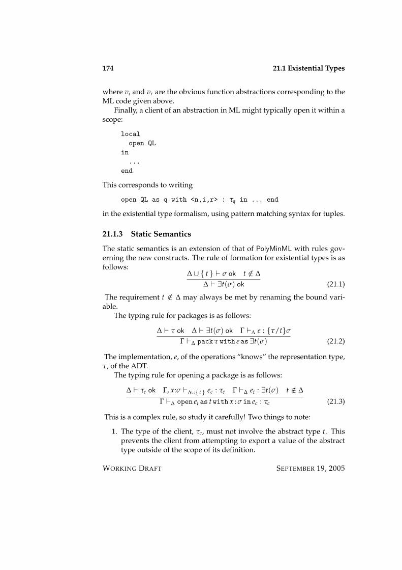
174 21.1 Existential Types
where vi and vr are the obvious function abstractions corresponding to theML code given above.
Finally, a client of an abstraction in ML might typically open it within ascope:
localopen QL
in...
end
This corresponds to writing
open QL as q with <n,i,r> : τq in ... end
in the existential type formalism, using pattern matching syntax for tuples.
21.1.3 Static Semantics
The static semantics is an extension of that of PolyMinML with rules gov-erning the new constructs. The rule of formation for existential types is asfollows:
∆ ∪ t ` σ ok t /∈ ∆∆ ` ∃t(σ) ok (21.1)
The requirement t /∈ ∆ may always be met by renaming the bound vari-able.
The typing rule for packages is as follows:
∆ ` τ ok ∆ ` ∃t(σ) ok Γ `∆ e : τ/tσΓ `∆ pack τ with e as ∃t(σ) (21.2)
The implementation, e, of the operations “knows” the representation type,τ, of the ADT.
The typing rule for opening a package is as follows:
∆ ` τc ok Γ, x:σ `∆∪ t ec : τc Γ `∆ ei : ∃t(σ) t /∈ ∆
Γ `∆ open ei as t with x:σ in ec : τc (21.3)
This is a complex rule, so study it carefully! Two things to note:
1. The type of the client, τc, must not involve the abstract type t. Thisprevents the client from attempting to export a value of the abstracttype outside of the scope of its definition.
WORKING DRAFT SEPTEMBER 19, 2005
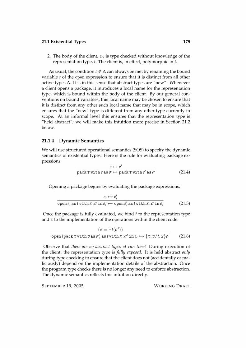
21.1 Existential Types 175
2. The body of the client, ec, is type checked without knowledge of therepresentation type, t. The client is, in effect, polymorphic in t.
As usual, the condition t /∈ ∆ can always be met by renaming the boundvariable t of the open expression to ensure that it is distinct from all otheractive types ∆. It is in this sense that abstract types are “new”! Whenevera client opens a package, it introduces a local name for the representationtype, which is bound within the body of the client. By our general con-ventions on bound variables, this local name may be chosen to ensure thatit is distinct from any other such local name that may be in scope, whichensures that the “new” type is different from any other type currently inscope. At an informal level this ensures that the representation type is“held abstract”; we will make this intuition more precise in Section 21.2below.
21.1.4 Dynamic Semantics
We will use structured operational semantics (SOS) to specify the dynamicsemantics of existential types. Here is the rule for evaluating package ex-pressions:
e 7→ e′
pack τ with e as σ 7→ pack τ with e′ as σ (21.4)
Opening a package begins by evaluating the package expressions:
ei 7→ e′iopen ei as t with x:σ in ec 7→ open e′i as t with x:σ in ec (21.5)
Once the package is fully evaluated, we bind t to the representation typeand x to the implementation of the operations within the client code:
(σ = ∃t(σ′))open (pack τ with v as σ) as t with x:σ′ in ec 7→ τ, v/t, xec (21.6)
Observe that there are no abstract types at run time! During execution ofthe client, the representation type is fully exposed. It is held abstract onlyduring type checking to ensure that the client does not (accidentally or ma-liciously) depend on the implementation details of the abstraction. Oncethe program type checks there is no longer any need to enforce abstraction.The dynamic semantics reflects this intuition directly.
SEPTEMBER 19, 2005 WORKING DRAFT

176 21.2 Representation Independence
21.1.5 Safety
The safety of the extension is stated and proved as usual. The argument isa simple extension of that used for PolyMinML to the new constructs.
Theorem 21.1 (Preservation)If e : τ and e 7→ e′, then e′ : τ.
Lemma 21.2 (Canonical Forms)If v : ∃t(σ) is a value, then v = pack τ with v′ as ∃t(σ) for some monotypeτ and some value v′ : τ/tσ.
Theorem 21.3 (Progress)If e : τ then either e value or there exists e′ such that e 7→ e′.
21.2 Representation Independence
Parametricity is the essence of representation independence. The typingrules for open given above ensure that the client of an abstract type is poly-morphic in the representation type. According to our informal understand-ing of parametricity this means that the client’s behavior is in some sense“independent” of the representation type.
More formally, we say that an (admissible) relation R : τ1 ↔ τ2 is abisimulation between the packages
pack τ1 with v1 as ∃t(σ)
andpack τ2 with v2 as ∃t(σ)
of type ∃t(σ) iff v1∼=val v2 : σ, taking equality at type t to be the relation
R. The reason for calling such a relation R a bisimulation will become ap-parent shortly. Two packages are said to be bisimilar whenever there is abisimulation between them.
Since the client ec of a data abstraction of type ∃t(σ) is essentially apolymorphic function of type ∀t(σ→τc), where t /∈ FTV(τc), it follows fromthe Parametricity Theorem that
τ1, v1/t, xec ∼=exp τ2, v2/t, xec : τc
whenever R is such a bisimulation. Consequently,
open e1 as t with x:σ in ec ∼=exp open e2 as t with x:σ in ec : τc.
WORKING DRAFT SEPTEMBER 19, 2005
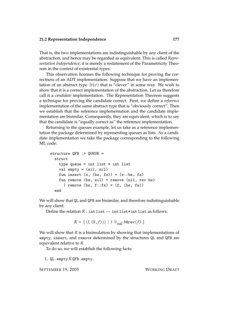
21.2 Representation Independence 177
That is, the two implementations are indistinguishable by any client of theabstraction, and hence may be regarded as equivalent. This is called Repre-sentation Independence; it is merely a restatement of the Parametricity Theo-rem in the context of existential types.
This observation licenses the following technique for proving the cor-rectness of an ADT implementation. Suppose that we have an implemen-tation of an abstract type ∃t(σ) that is “clever” in some way. We wish toshow that it is a correct implementation of the abstraction. Let us thereforecall it a candidate implementation. The Representation Theorem suggestsa technique for proving the candidate correct. First, we define a referenceimplementation of the same abstract type that is “obviously correct”. Thenwe establish that the reference implementation and the candidate imple-mentation are bisimilar. Consequently, they are equivalent, which is to saythat the candidate is “equally correct as” the reference implementation.
Returning to the queues example, let us take as a reference implemen-tation the package determined by representing queues as lists. As a candi-date implementation we take the package corresponding to the followingML code:
structure QFB :> QUEUE =structtype queue = int list * int listval empty = (nil, nil)fun insert (x, (bs, fs)) = (x::bs, fs)fun remove (bs, nil) = remove (nil, rev bs)| remove (bs, f::fs) = (f, (bs, fs))
end
We will show that QL and QFB are bisimilar, and therefore indistinguishableby any client.
Define the relation R : int list↔ int list*int list as follows:
R = (l, (b, f))) | l ∼=val b@rev( f)
We will show that R is a bisimulation by showing that implementations ofempty, insert, and remove determined by the structures QL and QFB areequivalent relative to R.
To do so, we will establish the following facts:
1. QL.empty R QFB.empty.
SEPTEMBER 19, 2005 WORKING DRAFT
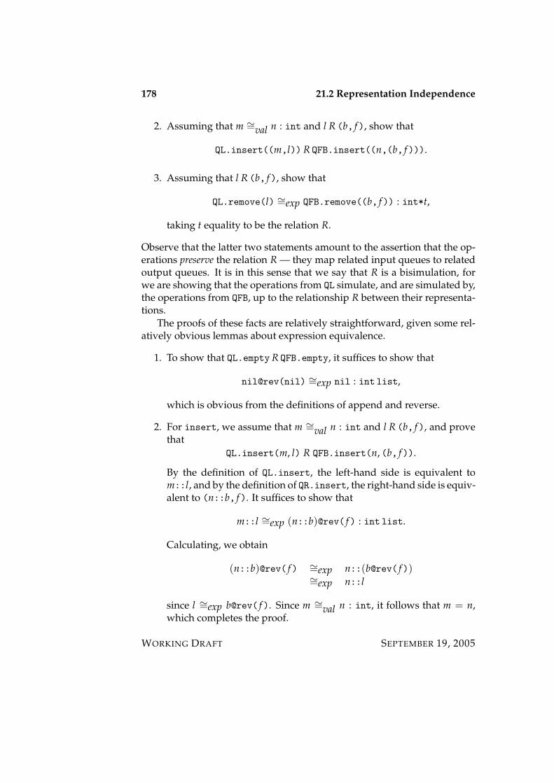
178 21.2 Representation Independence
2. Assuming that m ∼=val n : int and l R (b, f), show that
QL.insert((m,l)) R QFB.insert((n,(b, f))).
3. Assuming that l R (b, f), show that
QL.remove(l) ∼=exp QFB.remove((b, f)) : int*t,
taking t equality to be the relation R.
Observe that the latter two statements amount to the assertion that the op-erations preserve the relation R — they map related input queues to relatedoutput queues. It is in this sense that we say that R is a bisimulation, forwe are showing that the operations from QL simulate, and are simulated by,the operations from QFB, up to the relationship R between their representa-tions.
The proofs of these facts are relatively straightforward, given some rel-atively obvious lemmas about expression equivalence.
1. To show that QL.empty R QFB.empty, it suffices to show that
nil@rev(nil) ∼=exp nil : int list,
which is obvious from the definitions of append and reverse.
2. For insert, we assume that m ∼=val n : int and l R (b, f), and provethat
QL.insert(m, l) R QFB.insert(n, (b, f)).
By the definition of QL.insert, the left-hand side is equivalent tom::l, and by the definition of QR.insert, the right-hand side is equiv-alent to (n::b, f). It suffices to show that
m::l ∼=exp (n::b)@rev( f) : int list.
Calculating, we obtain
(n::b)@rev( f) ∼=exp n::(b@rev( f))∼=exp n::l
since l ∼=exp b@rev( f). Since m ∼=val n : int, it follows that m = n,which completes the proof.
WORKING DRAFT SEPTEMBER 19, 2005
21.2 Representation Independence 179
3. For remove, we assume that l is related by R to (b, f), which is to saythat l ∼=exp b@rev( f). We are to show
QL.remove(l) ∼=exp QFB.remove((b, f)) : int*t,
taking t equality to be the relation R. Assuming that the queue is non-empty, so that the remove is defined, we have l ∼=exp l′@[m] for somel′ and m. We proceed by cases according to whether or not f is empty.If f is non-empty, then f ∼=exp n:: f ′ for some n and f ′. Then by thedefinition of QFB.remove,
QFB.remove((b, f)) ∼=exp (n,(b, f ′)) : int*t,
relative to R. We must show that
(m,l′) ∼=exp (n,(b, f ′)) : int*t,
relative to R. This means that we must show that m = n and l′ ∼=expb@rev( f ′) : int list.
Calculating from our assumptions,
l = l′@[m]= b@rev( f)= b@rev(n:: f ′)= b@(rev( f ′)@[n])= (b@rev( f ′))@[n]
From this the result follows. Finally, if f is empty, then b ∼=exp b′@[n]for some b′ and n. But then rev(b) ∼=exp n::rev(b′), which reducesto the case for f non-empty.
This completes the proof — by Representation Independence the refer-ence and candidate implementations are equivalent.
SEPTEMBER 19, 2005 WORKING DRAFT

180 21.2 Representation Independence
WORKING DRAFT SEPTEMBER 19, 2005
Part VIII
Lazy Evaluation
181

Chapter 22
Lazy Types
The language MinML is an example of an eager, or strict, functional lan-guage. Such languages are characterized by two, separable features of theiroperational semantics.
1. Call-by-value. The argument to a function is evaluated before controlis passed to the body of the function. Function parameters are onlyever bound to values.
2. Strict data types. A value of a data type is constructed, possibly fromother values, at the point at which the constructor is used.
Since most familiar languages are eager, this might seem to be the mostnatural, or even the only possible, choice. The subject of this chapter isto explore an alternative, lazy evaluation, that seeks to delay evaluation ofexpressions as long as possible, until their value is actually required to com-plete a computation. This strategy is called “lazy” because we perform onlythe evaluation that is actually required to complete a computation. If thevalue of an expression is never required, it is never (needlessly) computed.Moreover, the lazy evaluation strategy memoizes delayed computations sothat they are never performed more than once. Once (if ever) the valuehas been determined, it is stored away to be used in case the value is everneeded again.
Lazy languages are characterized by the following features of their op-erational semantics.
1. Call-by-need. The argument to a function is passed to the body of thefunction without evaluating it. The argument is only evaluated if itis needed in the computation, and then its value is saved for futurereference in case it is needed again.
183

184
2. Lazy data types. An expression yielding a value of a data type is notevaluated until its value is actually required to complete a computa-tion. The value, once obtained, is saved in case it is needed again.
While it might seem, at first glance, that lazy evaluation would lead tomore efficient programs (by avoiding unnecessary work), it is not at all ob-vious that this is the case. In fact it’s not the case. The main issue is thatmemoization is costly, because of the bookkeeping overhead required tomanage the transition from unevaluated expression to evaluated value. Adelayed computation must store the code that determines the value of anexpression (should it be required), together with some means of triggeringits evaluation once it is required. If the value is ever obtained, the value de-termined by the code must be stored away, and we must somehow ensurethat this value is returned on subsequent access. This can slow down manyprograms. For example, if we know that a function will inspect the valueof every element of a list, it is much more efficient to simply evaluate theseelements when the list is created, rather than fruitlessly delaying the com-putation of each element, only to have it be required eventually anyway.Strictness analysis is used in an attempt to discover such cases, so that theoverhead can be eliminated, but in general it is impossible (for decidabilityreasons) to determine completely and accurately whether the value of anexpression is surely needed in a given program.
The real utility of lazy evaluation lies not in the possible efficiency gainsit may afford in some circumstances, but rather in a substantial increasein expressive power that it brings to a language. By delaying evaluationof an expression until it is needed, we can naturally model situations inwhich the value does not even exist until it is required. A typical exampleis interactive input. The user can be modelled as a “delayed computation”that produces its values (i.e., enters its input) only upon demand, not allat once before the program begins execution. Lazy evaluation models thisscenario quite precisely.
Another example of the use of lazy evaluation is in the representationof infinite data structures, such as the sequence of all natural numbers. Ob-viously we cannot hope to compute the entire sequence at the time that itis created. Fortunately, only a finite initial segment of the sequence is everneeded to complete execution of a program. Using lazy evaluation we cancompute this initial segment on demand, avoiding the need to compute thepart we do not require.
Lazy evaluation is an important and useful concept to have at your dis-posal. The question that we shall explore in this chapter is how best to
WORKING DRAFT SEPTEMBER 19, 2005
22.1 Lazy Types 185
provide such a feature in a programming language. Historically, there hasbeen a division between eager and lazy languages, exemplified by ML andHaskell, respectively, which impose one or the other evaluation strategyglobally, leaving no room for combining the best of both approaches.
More recently, it has come to be recognized by both communities thatit is important to support both forms of evaluation. This has led to two,distinct approaches to supporting laziness:
1. Lazy types in a strict language. The idea is to add support for lazydata types to a strict language by providing a means of defining suchtypes, and for creating and destroying values of these types. Con-structors are implicitly memoized to avoid redundant re-computationof expressions. The call-by-value evaluation strategy for functions ismaintained.
2. Strict types in a lazy language. The idea is to add support for construc-tors that forcibly evaluate their arguments, avoiding the overhead ofmanaging the bookkeeping associated with delayed, memoized com-putation. The call-by-need evaluation strategy for function calls ismaintained.
We will explore both alternatives.
22.1 Lazy Types
We will first explore the addition of lazy data types to a strict functionallanguage. We will focus on a specific example, the type of lazy lists. Forthe sake of simplicity we’ll consider only lazy lists of integers, but noth-ing hinges on this assumption.1 For the rest of this section we’ll drop themodifier “lazy”, and just write “list”, instead of “lazy list”.
The key idea is to treat a computation of a list element as a value of listtype, where a computation is simply a memoized, delayed evaluation ofan expression. By admitting computations as values we can support lazylists in a strict language. In particular the call-by-value evaluation strat-egy is not disrupted. Passing a lazy list to a function does not cause thedelayed computation to be evaluated; rather, it is passed in delayed form tothe function as a computation of that type. Pattern matching on a value oflist type requires that the computation be forced to expose the underlying
1It simply allows us to avoid forward-referencing the concept of polymorphism.
SEPTEMBER 19, 2005 WORKING DRAFT
186 22.1 Lazy Types
list element, which is then analyzed and deconstructed. It is very impor-tant to keep in mind the distinction between evaluation of an expression oflist type, and forcing a value of list type. The former simply yields a com-putation as value, whereas the latter evaluates and memoizes the delayedcomputation.
One consequence of laziness is that the tail of a (non-empty) lazy list,need not “exist” at the time the non-empty list is created. Being itself a lazylist, the tail need only be produced “on demand”, by forcing a computation.This is the key to using lazy lists to model interactive input and to representinfinite data structures. For example, we might define the infinite list ofnatural numbers by the equation
nats = iterate successor 0
where the function iterate is defined (informally) by the equation
iterate f x = lcons (x, iterate f (f x)),
where lcons creates a non-empty lazy list with the specified head and tail.We must think of nats as being created on demand. Successive elements ofnats are created by succcessive recursive calls to iterate, which are onlymade as we explore the list.
Another approach to defining the infinite list of natural numbers is tomake use of self-reference, as illustrated by the following example. The in-finite sequence of natural numbers may be thought as a solution to therecursion equation
nats = lcons (0, lmap successor nats),
where successor and lmap are the evident functions. Here again we mustthink of nats as being created on demand. Successive elements of natsare created as follows. When we inspect the first element of nats, it isimmediately revealed to be 0, as specified. When we inspect the secondelement, we apply lmap successor to nats, then inspect the head elementof the result. This is successor(0), or 1; it’s tail is the result of mappingsuccessor over that list — that is, the result of adding 2 to every elementof the original list, and so on.
WORKING DRAFT SEPTEMBER 19, 2005

22.1 Lazy Types 187
22.1.1 Lazy Lists in an Eager Language
The additional constructs required to add lazy lists to MinML are given bythe following grammar:
Types τ : : = llistExpressions e : : = lnil | lcons(e1,e2) | lazy x is e |
lcase e of lnil => e0 | lcons(x,y) => e1
In the expression lazy x is e the variable x is bound within e; in the ex-pression lcase e of lnil => e0 | lcons(x,y) => e1 the variables x and y arebound in e1. As usual we identify expressions that differ only in the namesof their bound variables.
Lazy lists may be defined either by explicit construction — using lniland lcons — or by a recursion equation — using lazy x is e, where e isa lazy list expression. The idea is that the variable x stands for the listconstructed by e, and may be used within e to refer to the list itself. Forexample, the infinite list of 1’s is given by the expression
lazy x is lcons(1,x).
More interesting examples can be expressed using recursive definitionssuch as the following definition of the list of all natural numbers:
lazy x is lcons (1, lmap successor x).
To complete this definition we must define lmap. This raises a subtle issuethat is very easy to overlook. A natural choice is as follows:
fun map(f:int->int):llist->llist isfun lmapf(l:llist) islcase l
of lnil => lnil| lcons(x,y) => lcons (f x, lmapf y).
Unfortunately this definition doesn’t work as expected! Suppose that fis a function of type int->int and that l is a non-empty lazy list. Con-sider what happens when we evaluate the expression map f l. The lcaseforces evaluation of l, which leads to a recursive call to the internal func-tion lmapf, which forces the evaluation of the tail of l, and so on. If l is aninfinite list, the application diverges.
The problem is that the result of a call to map f l should be representedby a computation of a list, in which subsequent calls to map on the tail(s) ofthat list are delayed until they are needed. This is achieved by the followingcoding trick:
SEPTEMBER 19, 2005 WORKING DRAFT
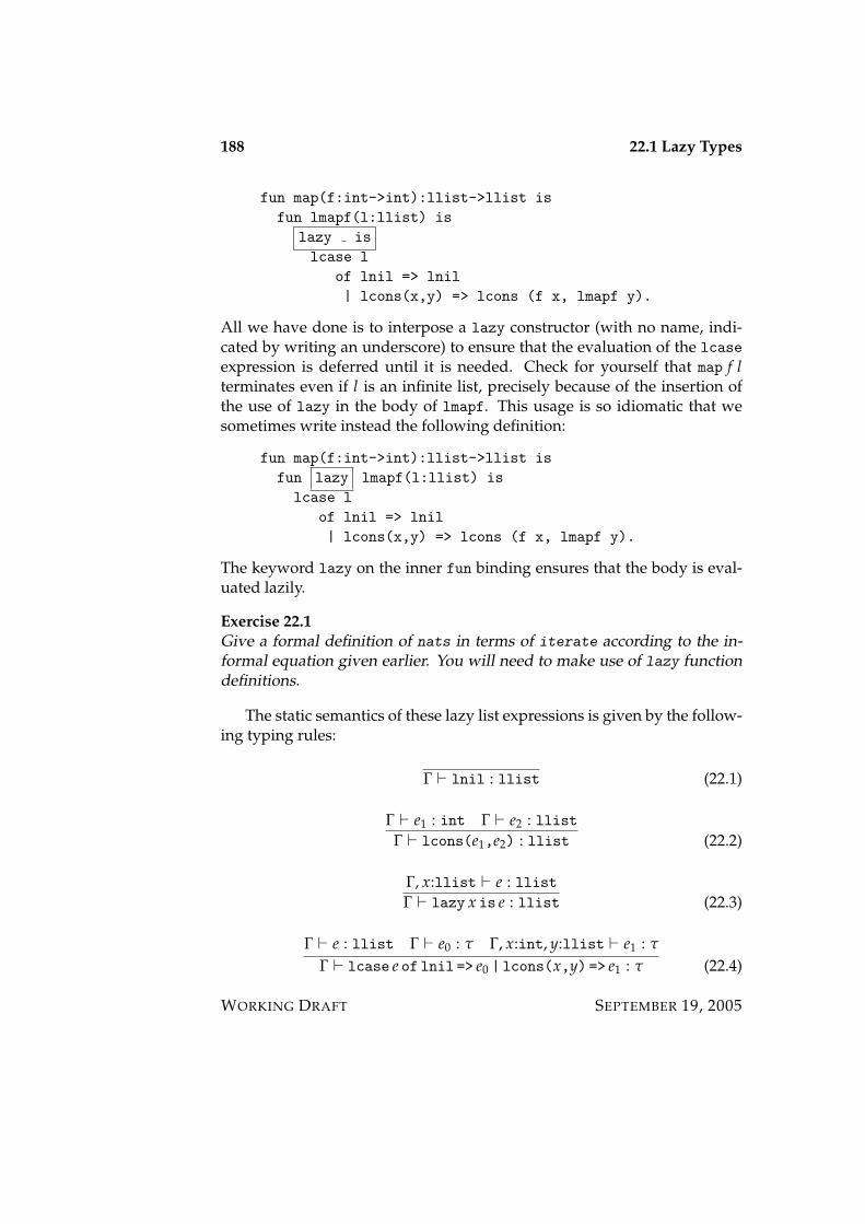
188 22.1 Lazy Types
fun map(f:int->int):llist->llist isfun lmapf(l:llist) is
lazy islcase l
of lnil => lnil| lcons(x,y) => lcons (f x, lmapf y).
All we have done is to interpose a lazy constructor (with no name, indi-cated by writing an underscore) to ensure that the evaluation of the lcaseexpression is deferred until it is needed. Check for yourself that map f lterminates even if l is an infinite list, precisely because of the insertion ofthe use of lazy in the body of lmapf. This usage is so idiomatic that wesometimes write instead the following definition:
fun map(f:int->int):llist->llist isfun lazy lmapf(l:llist) islcase l
of lnil => lnil| lcons(x,y) => lcons (f x, lmapf y).
The keyword lazy on the inner fun binding ensures that the body is eval-uated lazily.
Exercise 22.1Give a formal definition of nats in terms of iterate according to the in-formal equation given earlier. You will need to make use of lazy functiondefinitions.
The static semantics of these lazy list expressions is given by the follow-ing typing rules:
Γ ` lnil : llist (22.1)
Γ ` e1 : int Γ ` e2 : llistΓ ` lcons(e1,e2) : llist (22.2)
Γ, x:llist ` e : llistΓ ` lazy x is e : llist (22.3)
Γ ` e : llist Γ ` e0 : τ Γ, x:int, y:llist ` e1 : τ
Γ ` lcase e of lnil => e0 | lcons(x,y) => e1 : τ (22.4)
WORKING DRAFT SEPTEMBER 19, 2005
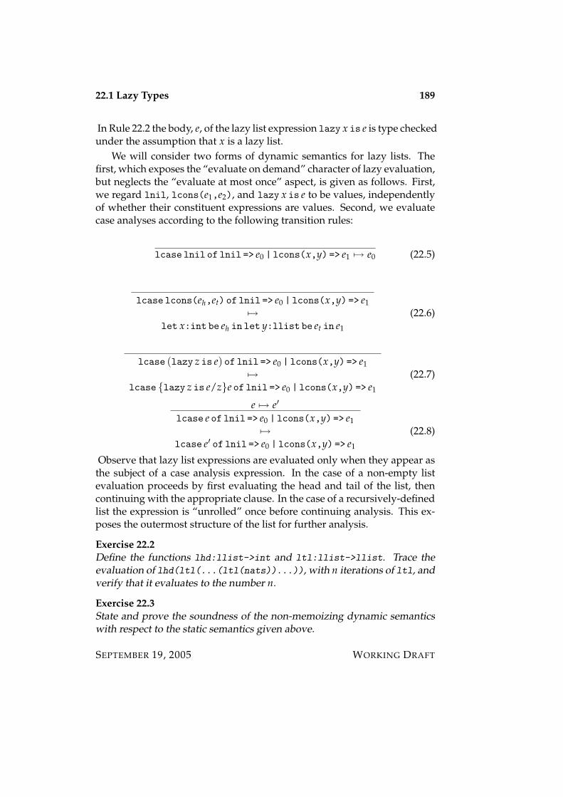
22.1 Lazy Types 189
In Rule 22.2 the body, e, of the lazy list expression lazy x is e is type checkedunder the assumption that x is a lazy list.
We will consider two forms of dynamic semantics for lazy lists. Thefirst, which exposes the “evaluate on demand” character of lazy evaluation,but neglects the “evaluate at most once” aspect, is given as follows. First,we regard lnil, lcons(e1,e2), and lazy x is e to be values, independentlyof whether their constituent expressions are values. Second, we evaluatecase analyses according to the following transition rules:
lcase lnil of lnil => e0 | lcons(x,y) => e1 7→ e0 (22.5)
lcase lcons(eh,et) of lnil => e0 | lcons(x,y) => e17→
let x:int be eh in let y:llist be et in e1
(22.6)
lcase (lazy z is e) of lnil => e0 | lcons(x,y) => e17→
lcase lazy z is e/ze of lnil => e0 | lcons(x,y) => e1
(22.7)
e 7→ e′
lcase e of lnil => e0 | lcons(x,y) => e17→
lcase e′ of lnil => e0 | lcons(x,y) => e1
(22.8)
Observe that lazy list expressions are evaluated only when they appear asthe subject of a case analysis expression. In the case of a non-empty listevaluation proceeds by first evaluating the head and tail of the list, thencontinuing with the appropriate clause. In the case of a recursively-definedlist the expression is “unrolled” once before continuing analysis. This ex-poses the outermost structure of the list for further analysis.
Exercise 22.2Define the functions lhd:llist->int and ltl:llist->llist. Trace theevaluation of lhd(ltl(...(ltl(nats))...)), with n iterations of ltl, andverify that it evaluates to the number n.
Exercise 22.3State and prove the soundness of the non-memoizing dynamic semanticswith respect to the static semantics given above.
SEPTEMBER 19, 2005 WORKING DRAFT

190 22.1 Lazy Types
Consider the lazy list value v = lazy x is x. It is easy to verify that eis well-typed, with type llist. It is also easy to see that performing a caseanalysis on v leads to an infinite regress, since v/xx = v. The value v isan example of a “black hole”, a value that, when forced, will lead back tothe value itself, and, moreover, is easily seen to lead to divergence. Anotherexample of a black hole is the value
lazy x is (lmap succ x)
that, when forced, maps the successor function over itself.What is it that makes the recursive list
lazy nats is lcons (0, lmap succ nats)
well-defined? This expression is not a black hole because the occurrence ofnats in the body of the recursive list expression is “guarded” by the call tolcons.
Exercise 22.4Develop a type discipline that rules out black holes as ill-formed. Hint:Define a judgement Γ ` e ↓ x, which means that x is guarded within e.Ensure that lazy x is e is well-typed only if x is guarded within e.
Exercise 22.5It is often convenient to define several lists simultaneously by mutual re-cursion. Generalize lazy x is e to admit simultaneous recursive definitionof several lists at once.
The foregoing dynamic semantics neglects the “evaluate at most once”aspect of laziness — if a lazy list expression is ever evaluated, its valueshould be stored so that re-evaluation is avoided should it ever be analyzedagain. This can be modeled by introducing a memory that holds delayedcomputations whenever they are created. The memory is updated if (andonly if) the value of that computation is ever required. Thus no evaluationis ever repeated, and some pending evaluations may never occur at all.This is called memoization.
The memoizing dynamic semantics is specified by an abstract machinewith states of the form (M, e), where M is a memory, a finite mapping ofvariables to values, and e is an expression whose free variables are all inthe domain of M. Free variables are used to stand for the values of listexpressions; they are essentially pointers into the memory, which storesthe value of the expression. We therefore regard free variables as values;these are in fact the only values of list type in this semantics.
WORKING DRAFT SEPTEMBER 19, 2005

22.1 Lazy Types 191
The transition rules for the memoizing dynamic semantics are as fol-lows:
(x /∈ dom(M))(M, lazy z is e) 7→ (M[x=lazy z is e], x) (22.9)
(x /∈ dom(M))(M, lnil) 7→ (M[x=lnil], x) (22.10)
(x /∈ dom(M))(M, lcons(e1,e2)) 7→ (M[x=lcons(e1,e2)], x) (22.11)
(M(z) = lnil)(M, lcase z of lnil => e0 | lcons(x,y) => e1)
7→(M, e0)
(22.12)
(M(z) = lcons(vh,vt))(M, lcase z of lnil => e0 | lcons(x,y) => e1) 7→ (M, vh, vt/x, ye1)
(22.13)
(M(z) = lcons(eh,et)) (M[z=•], eh) 7→∗ (M′, vh) (M′[z=•], et) 7→∗ (M′′, vt)(M, lcase z of lnil => e0 | lcons(x,y) => e1)
7→(M′′[z=lcons(vh,vt)], vh, vt/x, ye1)
(22.14)
(M(z) = lazy z is e) (M[z=•], e) 7→∗ (M′, v)(M, lcase z of lnil => e0 | lcons(x,y) => e1)
7→(M′[z=v], lcase v of lnil => e0 | lcons(x,y) => e1)
(22.15)
(M, e) 7→ (M′, e′)(M, lcase e of lnil => e0 | lcons(x,y) => e1)
7→(M′, lcase e′ of lnil => e0 | lcons(x,y) => e1)
(22.16)
Warning: These rules are very subtle! Here are some salient points tokeep in mind when studying them.
First, observe that the list-forming constructs are no longer values, butinstead have evaluation rules associated with them. These rules simply
SEPTEMBER 19, 2005 WORKING DRAFT

192 22.1 Lazy Types
store a pending computation in the memory and return a “pointer” to itas result. Thus a value of lazy list type is always a variable referring to apending computation in the store.
Second, observe that the rules for case analysis inspect the contents ofmemory to determine how to proceed. The case for lnil is entirely straight-forward, but the other two cases are more complex. Suppose that locationz contains lcons(e1,e2). First, we check whether we’ve already evaluatedthis list cell. If so, we continue by evaluating e1, with x and y replacedby the previously-computed values of the head and tail of the list. Other-wise, the time has come to evaluate this cell. We evaluate the head and tailcompletely to obtain their values, then continue by substituting these valuesfor the appropriate variables in the clause for non-empty lists. Moreover,we update the memory to record the values of the head and tail of the listso that subsequent accesses avoid re-evaluation. Similarly, if z contains arecursively-defined list, we fully evaluate its body, continuing with the re-sult and updating the memory to reflect the result of evaluation.
Third, we explicitly check for “black holes” by ensuring that a run-timeerror occurs whenever they are encountered. This is achieved by temporar-ily setting the contents of a list cell to the special “black hole” symbol,•, during evaluation of a list expression, thereby ensuring the evaluation“gets stuck” (i.e., incurs a run-time error) in the case that evaluation of a listexpression requires the value of the list itself.
Exercise 22.6Convince yourself that the replacement of z by • in the second premise ofRule 22.14 is redundant — the location z is already guaranteed to be boundto •.
Exercise 22.7State and prove the soundness of the memoizing dynamic semantics withrespect to the static semantics given above. Be certain that your treatmentof the memory takes account of cyclic dependencies.
Exercise 22.8Give an evaluation semantics for memoized lazy lists by a set of rules forderiving judgements of the form (M, e) ⇓ (M′, v).
Exercise 22.9Consider once again the augmented static semantics in which black holesare ruled out. Prove that evaluation never “gets stuck” by accessing a cellthat contains the black hole symbol.
WORKING DRAFT SEPTEMBER 19, 2005

22.1 Lazy Types 193
Exercise 22.10Consider again the definition of the natural numbers as the lazy list
lazy nats is (lcons (0, lmap succ nats)).
Prove that, for the non-memoized semantics, that accessing the nth elementrequires O(n2) time, whereas in the memoized semantics the same compu-tation requires O(n) time. This shows that memoization can improve theasymptotic complexity of an algorithm (not merely lower the constant fac-tors).
22.1.2 Delayed Evaluation and Lazy Data Structures
Another approach to lazy evaluation in the context of a strict language isto isolate the notion of a delayed computation as a separate concept. Thecrucial idea is that a delayed computation is a value that can, for example,appear in a component of a data structure. Evaluation of a delayed com-putation occurs as a result of an explicit force operation. Computations areimplicitly memoized in the sense that the first time it is forced, its value isstored and returned immediately should it ever be forced again. Lazy datastructures can then be built up using standard means, but with judicioususe of delayed computations to ensure laziness.
Since the technical details of delayed computation are very similar tothose just outlined for lazy lists, we will go through them only very briefly.Here is a syntactic extension to MinML that supports delayed evaluation:
Types τ : : = τ computationExpressions e : : = delay x is e | eval e1 as x in e2
In the expression delay x is e the variable x is bound within e, and in theexpression eval e1 as x in e2 the variable x is bound within e2. The ex-pression delay x is e both delays evaluation of e and gives it a name thatcan be used within e to stand for the computation itself. The expressioneval e1 as x in e2 forces the evaluation of the delayed computation e1, bindsthat value to x, and continues by evaluating e2.
The static semantics is given by the following rules:
Γ ` e : τΓ ` delay x is e : τ computation (22.17)
Γ ` e1 : τ1 computation Γ, x:τ1 ` e2 : τ2
Γ ` eval e1 as x in e2 : τ2 (22.18)
SEPTEMBER 19, 2005 WORKING DRAFT
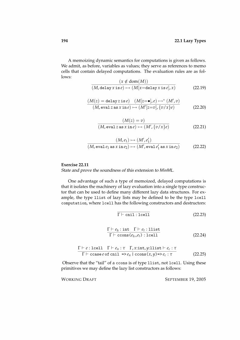
194 22.1 Lazy Types
A memoizing dynamic semantics for computations is given as follows.We admit, as before, variables as values; they serve as references to memocells that contain delayed computations. The evaluation rules are as fol-lows:
(x /∈ dom(M))(M, delay x is e) 7→ (M[x=delay x is e], x) (22.19)
(M(z) = delay z is e) (M[z=•], e) 7→∗ (M′, v)(M, eval z as x in e) 7→ (M′[z=v], v/xe) (22.20)
(M(z) = v)(M, eval z as x in e) 7→ (M′, v/xe) (22.21)
(M, e1) 7→ (M′, e′1)(M, eval e1 as x in e2) 7→ (M′, eval e′1 as x in e2) (22.22)
Exercise 22.11State and prove the soundness of this extension to MinML.
One advantage of such a type of memoized, delayed computations isthat it isolates the machinery of lazy evaluation into a single type construc-tor that can be used to define many different lazy data structures. For ex-ample, the type llist of lazy lists may be defined to be the type lcellcomputation, where lcell has the following constructors and destructors:
Γ ` cnil : lcell (22.23)
Γ ` eh : int Γ ` et : llistΓ ` ccons(eh,et) : lcell (22.24)
Γ ` e : lcell Γ ` en : τ Γ, x:int, y:llist ` ec : τ
Γ ` ccase e of cnil => en | ccons(x, y)=> ec : τ (22.25)
Observe that the “tail” of a ccons is of type llist, not lcell. Using theseprimitives we may define the lazy list constructors as follows:
WORKING DRAFT SEPTEMBER 19, 2005

22.1 Lazy Types 195
lnil = lazy is cnil
lcons(eh,et) = lazy is ccons(eh, et)
lcase e of nil => en | cons(x, y) => ec =force z=e incase z of cnil => en | ccons(x,y) => ec
Observe that case analysis on a lazy list forces the computation of that list,then analyzes the form of the outermost lazy list cell.
This “two-stage” construction of lazy lists in terms of lazy cells is oftenshort-circuited by simply identifying llist with lcell. However, this is amistake! The reason is that according to this definition every lazy list ex-pression must immediately determine whether the list is empty, and, if not,must determine its first element. But this conflicts with the “computationon demand” interpretation of laziness, according to which a lazy list mightnot even have a first element at the time that the list is defined, but only atthe time that the code inspects it. It is therefore imperative to distinguish,as we have done, between the type llist of lazy lists (delayed computa-tions of cells) and the type lcell of lazy cells (which specify emptiness anddefine the first element of non-empty lists).
SEPTEMBER 19, 2005 WORKING DRAFT

196 22.1 Lazy Types
WORKING DRAFT SEPTEMBER 19, 2005
Chapter 23
Lazy Languages
So far we’ve been considering the addition of lazy types to eager languages.Now we’ll consider the alternative, the notion of a lazy lanuage and, briefly,the addition of eager types to a lazy language.
As we said in the introduction the main features of a lazy language arethe call-by-need argument-passing discipline together with lazy value con-structors that construct values of a type from delayed computations. Undercall-by-value the arguments to functions and constructors are evaluatedbefore the function is called or the constructor is applied. Variables areonly ever bound to fully-evaluated expressions, or values, and construc-tors build values out of other values. Under call-by-need arguments arepassed to functions in delayed, memoized form, without evaluating themuntil they are needed. Moreover, value constructors build delayed, memo-ized computations out of other delayed, memoized computations, withoutevaluation. Variables are, in general, bound to pending computations thatare only forced when (and if) that value is required. Once forced, the bind-ing is updated to record the computed value, should it ever be requiredagain.
The interesting thing is that the static typing rules for the lazy variant ofMinML are exactly the same as those for the eager version. What is differ-ent is how those types are interpreted. In an eager language values of typeint are integer values (i.e., numbers); in a lazy language they are integercomputations, some of which might not even terminate when evaluated.Similarly, in an eager language values of list type are finite sequences ofvalues of the element type; in a lazy language values of list type are com-putations of such sequences, which need not be finite. And so on. Theimportant point is that the types have different meanings in lazy languages
197
198
than they do in strict languages.One symptom of this difference is that lazy languages are very liberal in
admitting recursive definitions compared to eager languages. In an eagerlanguage it makes no sense to admit recursive definitions such as
val x : int = 1+x
or
val x : int list = cons (1, x).
Roughly speaking, neither of these recursion equations has a solution. Thereis no integer value x satisfying the equation x = 1 + x, nor is there any finitelist satisfying the equation x = cons(1,x).
However, as we’ve already seen, equations such as
val x : int delayed = delay (1 + x)
and
val x : int list delayed = delay (lcons (1, x))
do make sense, precisely because they define recursive computations, ratherthan values. The first example defines a computation of an integer that,when forced, diverges; the second defines a computation of a list that, whenforced, computes a non-empty list with 1 as first element and the list itselfas tail.
In a lazy language every expression stands for a computation, so it isalways sensible to make a recursive definition such as
val rec x : int = 1+x.
Syntactically this looks like the inadmissible definition discussed above,but, when taken in the context of a lazy interpretation, it makes perfectsense as a definition of a recursive computation — the value of x is thedivergent computation of an integer.
The downside of admitting such a liberal treatment of computations isthat it leaves no room in the language for ordinary values! Everything’sa computation, with values emerging as those computations that happento have a trivial evaluation (e.g., numerals are trivial computations in thesense that no work is required to evaluate them). This is often touted asan advantage of lazy languages — the “freedom” to ignore whether some-thing is a value or not. But this appearance of freedom is really bondage.By admitting only computations, you are deprived of the ability to work
WORKING DRAFT SEPTEMBER 19, 2005

199
with plain values. For example, lazy languages do not have a type of nat-ural numbers, but rather only a type of computations of natural numbers.Consequently, elementary programming techniques such as definition bymathematical induction are precluded. The baby’s been thrown out withthe bathwater.
In recognition of this most lazy languages now admit eager types aswell as lazy types, moving them closer in spirit to eager languages thatadmit lazy types, but biased in the opposite direction. This is achieved ina somewhat unsatisfactory manner, by relying on data abstraction mecha-nisms to ensure that the only values of a type are those that are generatedby specified strict functions (those that evaluate their arguments). The rea-son it is unsatisfactory is that this approach merely limits the possible set ofcomputations of a given type, but still admits, for example, the undefinedcomputation as an element of every type.
23.0.3 Call-by-Name and Call-by-Need
To model lazy languages we simply extend MinML with an additional con-struct for recursively-defined computations, written rec x:τ is e. The vari-able x is bound in e, and may be renamed at will. Recursive computationsare governed by the following typing rule:
Γ, x:τ ` e : τ
Γ ` rec x:τ is e : τ (23.1)
In addition we replace the recursive function expression fun f (x:τ1):τ2 is ewith the non-recursive form fn τ:x in e, since the former may be defined bythe expression
rec f:τ1→τ2 is fn τ1:x in e.
As before, it is simpler to start with a non-memoizing dynamic seman-tics to better expose the core ideas. We’ll work with core MinML enrichedwith recursive computations. Closed values are precisely as for the eagercase, as are nearly all of the evaluation rules. The only exception is the rulefor function application, which is as follows:
fn τ:x in e(e′) 7→ fn τ:x in e, e′/xe (23.2)
This is known as the call-by-name1 rule, according to which arguments are
1The terminology is well-established, but not especially descriptive. As near as I can tellthe idea is that we pass the “name” of the computation (i.e., the expression that engendersit), rather than its value.
SEPTEMBER 19, 2005 WORKING DRAFT
200
passed to functions in unevaluated form, deferring their evaluation untilthe point at which they are actually used.
The only additional rule required is the one for recursive computations.But this is entirely straightforward:
rec x:τ is e 7→ rec x:τ is e/xe (23.3)
To evaluate a recursive computation, simply unroll the recursion by onestep and continue from there.
Exercise 23.1Show that the behavior of the recursive function expression fun f (x:τ1):τ2 is eis correctly defined by
rec f:τ1→τ2 is fn τ1:x in e
in the sense that an application of the latter mimicks the behavior of theformer (under call-by-name).
To model the “at most once” aspect of lazy evaluation we introduce,as before, a memory in which we store computations, initially in their un-evaluated, and later, if ever, in their evaluated forms. The difference hereis that all expressions define computations that must be stored. Since themain ideas are similar to those used to define lazy lists, we simply give theevaluation rules here.
The state of computation is a pair (M, e) where M is a finite memorymapping variables to values, and e is an expression whose free variableslie within the domain of M. Final states have the form (M, v), where v is aclosed value. In particular, v is not a variable.
Nearly all of the rules of MinML carry over to the present case nearly un-changed, apart from propagating the memory appropriately. For example,the rules for evaluating addition expressions is as follows:
(M, e1) 7→ (M′, e′1)(M, +(e1, e2)) 7→ (M′, +(e′1, e2)) (23.4)
(M, e2) 7→ (M′, e′2)(M, +(v1, e2)) 7→ (M′, +(v1, e′2)) (23.5)
(M, +(n1, n2)) 7→ (M, n1 + n2) (23.6)
WORKING DRAFT SEPTEMBER 19, 2005

201
The main differences are in the rule for function application and theneed for additional rules for variables and recursive computations.
(x /∈ dom(M))(M, fn τ:x in e(e′)) 7→ (M[x = e′], e) (23.7)
(M(x) = v)(M, x) 7→ (M, v) (23.8)
(M(x) = e) (M[x = •], e) 7→∗ (M′, v)(M, x) 7→ (M′[x = v], v) (23.9)
(x /∈ dom(M))(M, rec x:τ is e) 7→ (M[x = e], e) (23.10)
Observe that we employ the “black holing” technique to catch ill-definedrecursive definitions.
23.0.4 Strict Types in a Lazy Language
As discussed above, lazy languages are committed to the fundamental prin-ciple that the elements of a type are computations, which include values,and not just values themselves. This means, in particular, that every typecontains a “divergent” element, the computation that, when evaluated,goes into an infinite loop.2
One consequence, alluded to above, is that recursive type equationshave overly rich solutions. For example, in this setting the recursive typeequation
data llist = lnil | lcons of int * list
does not correspond to the familiar type of finite integer lists. In fact thistype contains as elements both divergent computations of lists and also
2This is often called “bottom”, written ⊥, for largely historical reasons. I prefer to avoidthis terminology because so much confusion has been caused by it. In particular, it is notalways correct to identify the least element of a domain with the divergent computation ofthat type! The domain of values of partial function type contains a least element, the totallyundefined function, but this element does not correspond to the divergent computation ofthat type.
SEPTEMBER 19, 2005 WORKING DRAFT
202
computations of infinite lists. The reason is that the tail of every list is acomputation of another list, so we can easily use recursion equations suchas
rec ones is lcons (1, ones)
to define an infinite element of this type.The inclusion of divergent expressions in every type is unavoidable in
a lazy language, precisely because of the commitment to the interpretationof types as computations. However, we can rule out infinite lists (for ex-ample) by insisting that cons evaluate its tail whenever it is applied. Thisis called a strictness annotation. If cons is strict in its seond argument, thenthe equation
rec ones is cons (1, ones)
denotes the divergent computation, rather than the infinite list of ones.These informal ideas correspond to different rules for evaluating con-
structors. We will illustrate this by giving a non-memoizing semantics forlazy MinML extended with eager lists. It is straightforward to adapt this tothe memoizing case.
In the fully lazy case the rules for evaluation are these. First, we regardlnil as a value, and regard lcons(e1,e2) as a value, regardless of whethere1 or e2 are values. Then we define the transition rules for case analysis asfollows:
lcase lnil of lnil => en | lcons(x,y) => ec 7→ en (23.11)
lcase lcons(e1,e2) of lnil => en | lcons(x,y) => ec 7→ e1, e2/x, yec(23.12)
If instead we wish to rule out infinite lists, then we may choose to regardlcons(e1,e2) to be a value only if e2 is a value, without changing the rulesfor case analysis. If we wish the elements of the list to be values, then weconsider lcons(e1,e2) to be a value only in the case that e1 is a value, andso on for all the possible combinations of choices.
As we stated earlier, this cuts down the set of possible computations of,say, list type, but retains the fundamental commitment to the interpretationof all types as types of computations.
WORKING DRAFT SEPTEMBER 19, 2005
Part IX
Dynamic Typing
203

Chapter 24
Dynamic Typing
The formalization of type safety given in Chapter 10 states that a languageis type safe iff it satisfies both preservation and progress. According to thisaccount, “stuck” states — non-final states with no transition — must berejected by the static type system as ill-typed. Although this requirementseems natural for relatively simple languages such as MinML, it is not im-mediately clear that our formalization of type safety scales to larger lan-guages, nor is it entirely clear that the informal notion of safety is faithfullycaptured by the preservation and progress theorems.
One issue that we addressed in Chapter 10 was how to handle expres-sions such as 3 div 0, which are well-typed, yet stuck, in apparent vio-lation of the progress theorem. We discussed two possible ways to handlesuch a situation. One is to enrich the type system so that such an expressionis ill-typed. However, this takes us considerably beyond the capabilities ofcurrent type systems for practical programming languages. The alternativeis to ensure that such ill-defined states are not “stuck”, but rather make atransition to a designated error state. To do so we introduced the notionof a checked error, which is explicitly detected and signalled during exe-cution. Checked errors are constrasted with unchecked errors, which areruled out by the static semantics.
In this chapter we will concern ourselves with question of why thereshould unchecked errors at all. Why aren’t all errors, including type er-rors, checked at run-time? Then we can dispense with the static semanticsentirely, and, in the process, execute more programs. Such a language iscalled dynamically typed, in contrast to MinML, which is statically typed.
One advantage of dynamic typing is that it supports a more flexibletreatment of conditionals. For example, the expression
205
206
(if true then 7 else "7")+1
is statically ill-typed, yet it executes successfully without getting stuck orincurring a checked error. Why rule it out, simply because the type checkeris unable to “prove” that the else branch cannot be taken? Instead we mayshift the burden to the programmer, who is required to maintain invari-ants that ensure that no run-time type errors can occur, even though theprogram may contain conditionals such as this one.
Another advantage of dynamic typing is that it supports heterogeneousdata structures, which may contain elements of many different types. Forexample, we may wish to form the “list”
[true, 1, 3.4, fn x=>x]
consisting of four values of distinct type. Languages such as ML precludeformation of such a list, insisting instead that all elements have the sametype; these are called homogenous lists. The argument for heterogeneity isthat there is nothing inherently “wrong” with such a list, particularly sinceits constructors are insensitive to the types of the components — they sim-ply allocate a new node in the heap, and initialize it appropriately.
Note, however, that the additional flexibility afforded by dynamic typ-ing comes at a cost. Since we cannot accurately predict the outcome ofa conditional branch, nor the type of a value extracted from a heteroge-neous data structure, we must program defensively to ensure that nothingbad happens, even in the case of a type error. This is achieved by turn-ing type errors into checked errors, thereby ensuring progress and hencesafety, even in the absence of a static type discipline. Thus dynamic typingcatches type errors as late as possible in the development cycle, whereasstatic typing catches them as early as possible.
In this chapter we will investigate a dynamically typed variant of MinMLin which type errors are treated as checked errors at execution time. Ouranalysis will reveal that, rather than being opposite viewpoints, dynamictyping is a special case of static typing! In this sense static typing is moreexpressive than dynamic typing, despite the superficial impression createdby the examples given above. This viewpoint illustrates the pay-as-you-goprinciple of language design, which states that a program should only in-cur overhead for those language features that it actually uses. By viewingdynamic typing as a special case of static typing, we may avail ourselves ofthe benefits of dynamic typing whenever it is required, but avoid its costswhenever it is not.
WORKING DRAFT SEPTEMBER 19, 2005

24.1 Dynamic Typing 207
24.1 Dynamic Typing
The fundamental idea of dynamic typing is to regard type clashes as checked,rather than unchecked, errors. Doing so puts type errors on a par with divi-sion by zero and other checked errors. This is achieved by augmenting thedynamic semantics with rules that explicitly check for stuck states. For ex-ample, the expression true+7 is such an ill-typed, stuck state. By checkingthat the arguments of an addition are integers, we can ensure that progressmay be made, namely by making a transition to error.
The idea is easily illustrated by example. Consider the rules for func-tion application in MinML given in Chapter 9, which we repeat here forconvenience:
v value v1 value (v = fun f (x:τ1):τ2 is e)apply(v, v1) 7→ v, v1/ f , xe
e1 7→ e′1apply(e1, e2) 7→ apply(e′1, e2)
v1 value e2 7→ e′2apply(v1, e2) 7→ apply(v1, e′2)
In addition to these rules, which govern the well-typed case, we addthe following rules governing the ill-typed case:
v value v1 value (v 6= fun f (x:τ1):τ2 is e)apply(v, v1) 7→ error
apply(error, e2) 7→ error
v1 value
apply(v1, error) 7→ error
The first rule states that a run-time error arises from any attempt to applya non-function to an argument. The other two define the propagation ofsuch errors through other expressions — once an error occurs, it propagatesthroughout the entire program.
By entirely analogous means we may augment the rest of the semanticsof MinML with rules to check for type errors at run time. Once we havedone so, it is safe to eliminate the static semantics in its entirety.1 Having
1We may then simplify the language by omitting type declarations on variables andfunctions, since these are no longer of any use.
SEPTEMBER 19, 2005 WORKING DRAFT
208 24.2 Implementing Dynamic Typing
done so, every expression is well-formed, and hence preservation holdsvacuously. More importantly, the progress theorem also holds because wehave augmented the dynamic semantics with transitions from every ill-typed expression to error, ensuring that there are no “stuck” states. Thus,the dynamically typed variant of MinML is safe in same sense as the stati-cally typed variant. The meaning of safety does not change, only the meansby which it is achieved.
24.2 Implementing Dynamic Typing
Since both the statically- and the dynamically typed variants of MinML aresafe, it is natural to ask which is better. The main difference is in how earlyerrors are detected — at compile time for static languages, at run time fordynamic languages. Is it better to catch errors early, but rule out someuseful programs, or catch them late, but admit more programs? Ratherthan attempt to settle this question, we will sidestep it by showing thatthe apparent dichotomy between static and dynamic typing is illusory byshowing that dynamic typing is a mode of use of static typing. From thispoint of view static and dynamic typing are matters of design for a par-ticular program (which to use in a given situation), rather than a doctrinaldebate about the design of a programming language (which to use in allsituations).
To see how this is possible, let us consider what is involved in imple-menting a dynamically typed language. The dynamically typed variant ofMinML sketched above includes rules for run-time type checking. For ex-ample, the dynamic semantics includes a rule that explicitly checks for anattempt to apply a non-function to an argument. How might such a checkbe implemented? The chief problem is that the natural representations ofdata values on a computer do not support such tests. For example, a func-tion might be represented as a word representing a pointer to a region ofmemory containing a sequence of machine language instructions. An in-teger might be represented as a word interpreted as a two’s complementinteger. But given a word, you cannot tell, in general, whether it is an inte-ger or a code pointer.
To support run-time type checking, we must adulterate our data rep-resentations to ensure that it is possible to implement the required checks.We must be able to tell by looking at the value whether it is an integer, aboolean, or a function. Having done so, we must be able to recover the un-derlying value (integer, boolean, or function) for direct calculation. When-
WORKING DRAFT SEPTEMBER 19, 2005
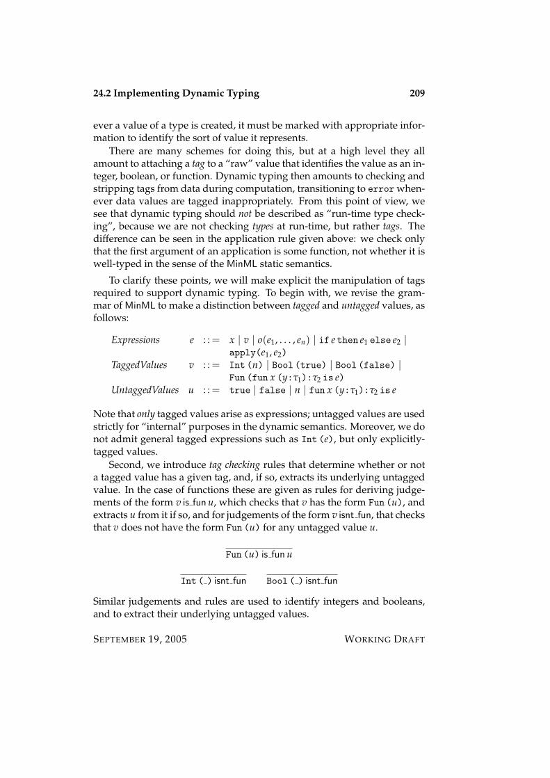
24.2 Implementing Dynamic Typing 209
ever a value of a type is created, it must be marked with appropriate infor-mation to identify the sort of value it represents.
There are many schemes for doing this, but at a high level they allamount to attaching a tag to a “raw” value that identifies the value as an in-teger, boolean, or function. Dynamic typing then amounts to checking andstripping tags from data during computation, transitioning to error when-ever data values are tagged inappropriately. From this point of view, wesee that dynamic typing should not be described as “run-time type check-ing”, because we are not checking types at run-time, but rather tags. Thedifference can be seen in the application rule given above: we check onlythat the first argument of an application is some function, not whether it iswell-typed in the sense of the MinML static semantics.
To clarify these points, we will make explicit the manipulation of tagsrequired to support dynamic typing. To begin with, we revise the gram-mar of MinML to make a distinction between tagged and untagged values, asfollows:
Expressions e : : = x | v | o(e1, . . . , en) | if e then e1 else e2 |apply(e1, e2)
TaggedValues v : : = Int (n) | Bool (true) | Bool (false) |Fun (fun x (y:τ1):τ2 is e)
UntaggedValues u : : = true | false | n | fun x (y:τ1):τ2 is e
Note that only tagged values arise as expressions; untagged values are usedstrictly for “internal” purposes in the dynamic semantics. Moreover, we donot admit general tagged expressions such as Int (e), but only explicitly-tagged values.
Second, we introduce tag checking rules that determine whether or nota tagged value has a given tag, and, if so, extracts its underlying untaggedvalue. In the case of functions these are given as rules for deriving judge-ments of the form v is fun u, which checks that v has the form Fun (u), andextracts u from it if so, and for judgements of the form v isnt fun, that checksthat v does not have the form Fun (u) for any untagged value u.
Fun (u) is fun u
Int ( ) isnt fun Bool ( ) isnt fun
Similar judgements and rules are used to identify integers and booleans,and to extract their underlying untagged values.
SEPTEMBER 19, 2005 WORKING DRAFT
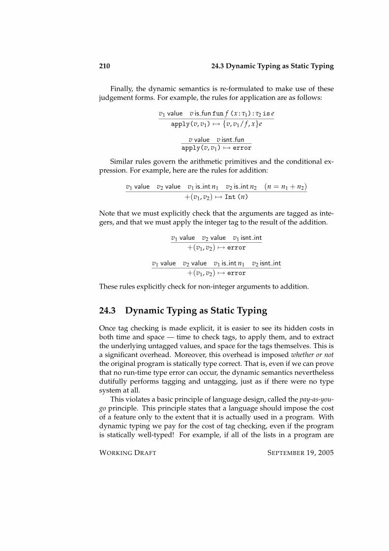
210 24.3 Dynamic Typing as Static Typing
Finally, the dynamic semantics is re-formulated to make use of thesejudgement forms. For example, the rules for application are as follows:
v1 value v is fun fun f (x:τ1):τ2 is eapply(v, v1) 7→ v, v1/ f , xe
v value v isnt funapply(v, v1) 7→ error
Similar rules govern the arithmetic primitives and the conditional ex-pression. For example, here are the rules for addition:
v1 value v2 value v1 is int n1 v2 is int n2 (n = n1 + n2)+(v1, v2) 7→ Int (n)
Note that we must explicitly check that the arguments are tagged as inte-gers, and that we must apply the integer tag to the result of the addition.
v1 value v2 value v1 isnt int
+(v1, v2) 7→ error
v1 value v2 value v1 is int n1 v2 isnt int
+(v1, v2) 7→ error
These rules explicitly check for non-integer arguments to addition.
24.3 Dynamic Typing as Static Typing
Once tag checking is made explicit, it is easier to see its hidden costs inboth time and space — time to check tags, to apply them, and to extractthe underlying untagged values, and space for the tags themselves. This isa significant overhead. Moreover, this overhead is imposed whether or notthe original program is statically type correct. That is, even if we can provethat no run-time type error can occur, the dynamic semantics neverthelessdutifully performs tagging and untagging, just as if there were no typesystem at all.
This violates a basic principle of language design, called the pay-as-you-go principle. This principle states that a language should impose the costof a feature only to the extent that it is actually used in a program. Withdynamic typing we pay for the cost of tag checking, even if the programis statically well-typed! For example, if all of the lists in a program are
WORKING DRAFT SEPTEMBER 19, 2005

24.3 Dynamic Typing as Static Typing 211
homogeneous, we should not have to pay the overhead of supporting het-erogeneous lists. The choice should be in the hands of the programmer, notthe language designer.
It turns out that we can eat our cake and have it too! The key is a simple,but powerful, observation: dynamic typing is but a mode of use of statictyping, provided that our static type system includes a type of tagged data!Dynamic typing emerges as a particular style of programming with taggeddata.
The point is most easily illustrated using ML. The type of tagged datavalues for MinML may be introduced as follows:
(* The type of tagged values. *)datatype tagged =Int of int |Bool of bool |Fun of tagged -> tagged
Values of type tagged are marked with a value constructor indicating theiroutermost form. Tags may be manipulated using pattern matching.
Second, we introduce operations on tagged data values, such as addi-tion or function call, that explicitly check for run-time type errors.
exception TypeError
fun checked add (m:tagged, n:tagged):tagged =case (m,n) of(Int a, Int b) => Int (a+b)
| ( , ) => raise TypeError
fun checked apply (f:tagged, a:tagged):tagged =case f ofFun g => g a
| => raise TypeError
Observe that these functions correspond precisely to the instrumented dy-namic semantics given above.
Using these operations, we can then build heterogeneous lists as valuesof type tagged list.
val het list : tagged list =[Int 1, Bool true, Fun (fn x => x)]
val f : tagged = hd(tl(tl het list))
val x : tagged = checked apply (f, Int 5)
SEPTEMBER 19, 2005 WORKING DRAFT
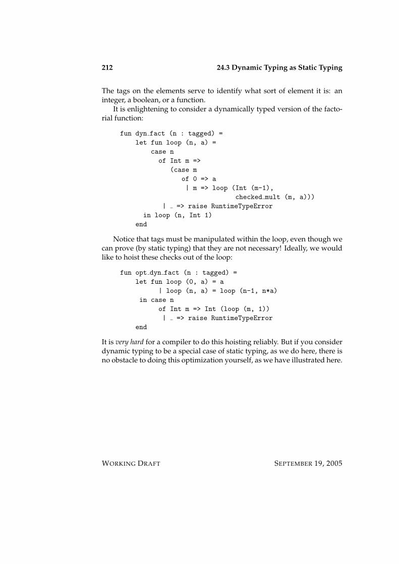
212 24.3 Dynamic Typing as Static Typing
The tags on the elements serve to identify what sort of element it is: aninteger, a boolean, or a function.
It is enlightening to consider a dynamically typed version of the facto-rial function:
fun dyn fact (n : tagged) =let fun loop (n, a) =
case nof Int m =>
(case mof 0 => a| m => loop (Int (m-1),
checked mult (m, a)))| => raise RuntimeTypeError
in loop (n, Int 1)end
Notice that tags must be manipulated within the loop, even though wecan prove (by static typing) that they are not necessary! Ideally, we wouldlike to hoist these checks out of the loop:
fun opt dyn fact (n : tagged) =let fun loop (0, a) = a
| loop (n, a) = loop (n-1, n*a)in case n
of Int m => Int (loop (m, 1))| => raise RuntimeTypeError
end
It is very hard for a compiler to do this hoisting reliably. But if you considerdynamic typing to be a special case of static typing, as we do here, there isno obstacle to doing this optimization yourself, as we have illustrated here.
WORKING DRAFT SEPTEMBER 19, 2005

Chapter 25
Featherweight Java
We will consider a tiny subset of the Java language, called FeatherweightJava, or FJ, that models subtyping and inheritance in Java. We will thendiscuss design alternatives in the context of FJ. For example, in FJ, as inJava, the subtype relation is tightly coupled to the subclass relation. Is thisnecessary? Is it desirable? We will also use FJ as a framework for dis-cussing other aspects of Java, including interfaces, privacy, and arrays.
25.1 Abstract Syntax
The abstract syntax of FJ is given by the following grammar:
Classes C : : = class c extends c c f; k dConstructors k : : = c(c x) super(x); this. f=x;Methods d : : = c m(c x) return e;Types τ : : = cExpressions e : : = x | e. f | e.m(e) | new c(e) | (c) e
The variable f ranges over a set of field names, c over a set of class names, mover a set of method names, and x over a set of variable names. We assumethat these sets are countably infinite and pairwise disjoint. We assume thatthere is a distinguished class name, Object, standing for the root of theclass hierarchy. It’s role will become clear below. We assume that there isa distinguished variable this that cannot otherwise be declared in a pro-gram.
As a notational convenience we use “underbarring” to stand for se-quences of phrases. For example, d stands for a sequence of d’s, whose
213
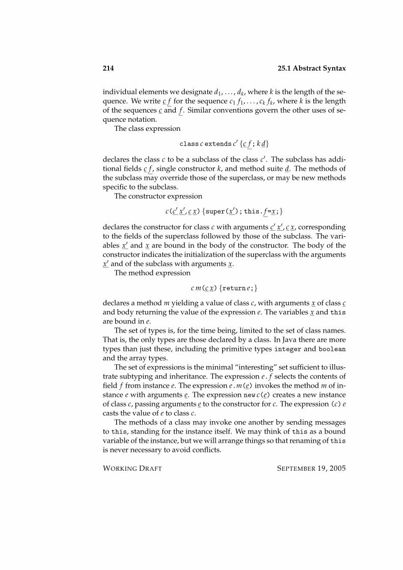
214 25.1 Abstract Syntax
individual elements we designate d1, . . . , dk, where k is the length of the se-quence. We write c f for the sequence c1 f1, . . . , ck fk, where k is the lengthof the sequences c and f . Similar conventions govern the other uses of se-quence notation.
The class expression
class c extends c′ c f; k d
declares the class c to be a subclass of the class c′. The subclass has addi-tional fields c f , single constructor k, and method suite d. The methods ofthe subclass may override those of the superclass, or may be new methodsspecific to the subclass.
The constructor expression
c(c′ x′, c x) super(x′); this. f=x;
declares the constructor for class c with arguments c′ x′, c x, correspondingto the fields of the superclass followed by those of the subclass. The vari-ables x′ and x are bound in the body of the constructor. The body of theconstructor indicates the initialization of the superclass with the argumentsx′ and of the subclass with arguments x.
The method expression
c m(c x) return e;
declares a method m yielding a value of class c, with arguments x of class cand body returning the value of the expression e. The variables x and thisare bound in e.
The set of types is, for the time being, limited to the set of class names.That is, the only types are those declared by a class. In Java there are moretypes than just these, including the primitive types integer and booleanand the array types.
The set of expressions is the minimal “interesting” set sufficient to illus-trate subtyping and inheritance. The expression e. f selects the contents offield f from instance e. The expression e.m(e) invokes the method m of in-stance e with arguments e. The expression new c(e) creates a new instanceof class c, passing arguments e to the constructor for c. The expression (c) ecasts the value of e to class c.
The methods of a class may invoke one another by sending messagesto this, standing for the instance itself. We may think of this as a boundvariable of the instance, but we will arrange things so that renaming of thisis never necessary to avoid conflicts.
WORKING DRAFT SEPTEMBER 19, 2005
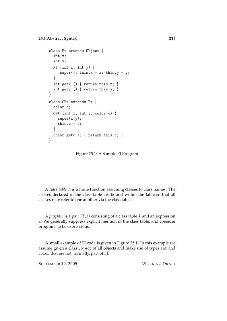
25.1 Abstract Syntax 215
class Pt extends Object int x;int y;
Pt (int x, int y) super(); this.x = x; this.y = y;
int getx () return this.x; int gety () return this.y;
class CPt extends Pt color c;
CPt (int x, int y, color c) super(x,y);this.c = c;
color getc () return this.c;
Figure 25.1: A Sample FJ Program
A class table T is a finite function assigning classes to class names. Theclasses declared in the class table are bound within the table so that allclasses may refer to one another via the class table.
A program is a pair (T, e) consisting of a class table T and an expressione. We generally suppress explicit mention of the class table, and considerprograms to be expressions.
A small example of FJ code is given in Figure 25.1. In this example weassume given a class Object of all objects and make use of types int andcolor that are not, formally, part of FJ.
SEPTEMBER 19, 2005 WORKING DRAFT

216 25.2 Static Semantics
25.2 Static Semantics
The static semantics of FJ is defined by a collection of judgments of thefollowing forms:
τ <: τ′ subtypingΓ ` e : τ expression typingd ok in c well-formed methodC ok well-formed classT ok well-formed class tablefields(c) = c f field lookuptype(m, c) = c→ c method type
The rules defining the static semantics follow.Every variable must be declared:
Γ(x) = τ
Γ ` x : τ (25.1)
The types of fields are defined in the class table.
Γ ` e0 : c0 fields(c0) = c f
Γ ` e0. fi : ci (25.2)
The argument and result types of methods are defined in the class table.
Γ ` e0 : c0 Γ ` e : ctype(m, c0) = c′ → c c <: c′
Γ ` e0.m(e) : c (25.3)
Instantiation must provide values for all instance variables as argu-ments to the constructor.
Γ ` e : c c <: c′ fields(c) = c′ f
Γ ` new c(e) : c (25.4)
All casts are statically valid, but must be checked at run-time.
Γ ` e0 : dΓ ` (c) e0 : c (25.5)
WORKING DRAFT SEPTEMBER 19, 2005
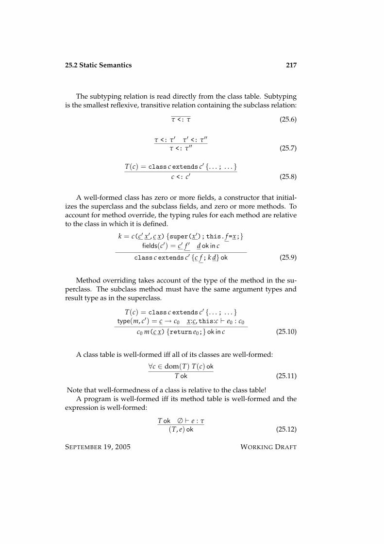
25.2 Static Semantics 217
The subtyping relation is read directly from the class table. Subtypingis the smallest reflexive, transitive relation containing the subclass relation:
τ <: τ (25.6)
τ <: τ′ τ′ <: τ′′
τ <: τ′′ (25.7)
T(c) = class c extends c′ . . . ; . . . c <: c′ (25.8)
A well-formed class has zero or more fields, a constructor that initial-izes the superclass and the subclass fields, and zero or more methods. Toaccount for method override, the typing rules for each method are relativeto the class in which it is defined.
k = c(c′ x′, c x) super(x′); this. f=x;fields(c′) = c′ f ′ d ok in c
class c extends c′ c f; k d ok (25.9)
Method overriding takes account of the type of the method in the su-perclass. The subclass method must have the same argument types andresult type as in the superclass.
T(c) = class c extends c′ . . . ; . . . type(m, c′) = c→ c0 x:c, this:c ` e0 : c0
c0 m(c x) return e0; ok in c (25.10)
A class table is well-formed iff all of its classes are well-formed:
∀c ∈ dom(T) T(c) ok
T ok (25.11)
Note that well-formedness of a class is relative to the class table!A program is well-formed iff its method table is well-formed and the
expression is well-formed:
T ok ∅ ` e : τ(T, e) ok (25.12)
SEPTEMBER 19, 2005 WORKING DRAFT
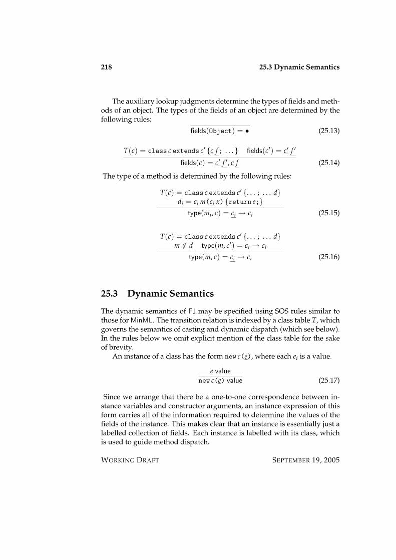
218 25.3 Dynamic Semantics
The auxiliary lookup judgments determine the types of fields and meth-ods of an object. The types of the fields of an object are determined by thefollowing rules:
fields(Object) = • (25.13)
T(c) = class c extends c′ c f; . . . fields(c′) = c′ f ′
fields(c) = c′ f ′, c f (25.14)
The type of a method is determined by the following rules:
T(c) = class c extends c′ . . . ; . . . ddi = ci m(ci x) return e;
type(mi, c) = ci → ci (25.15)
T(c) = class c extends c′ . . . ; . . . dm /∈ d type(m, c′) = ci → ci
type(m, c) = ci → ci (25.16)
25.3 Dynamic Semantics
The dynamic semantics of FJ may be specified using SOS rules similar tothose for MinML. The transition relation is indexed by a class table T, whichgoverns the semantics of casting and dynamic dispatch (which see below).In the rules below we omit explicit mention of the class table for the sakeof brevity.
An instance of a class has the form new c(e), where each ei is a value.
e value
new c(e) value (25.17)
Since we arrange that there be a one-to-one correspondence between in-stance variables and constructor arguments, an instance expression of thisform carries all of the information required to determine the values of thefields of the instance. This makes clear that an instance is essentially just alabelled collection of fields. Each instance is labelled with its class, whichis used to guide method dispatch.
WORKING DRAFT SEPTEMBER 19, 2005
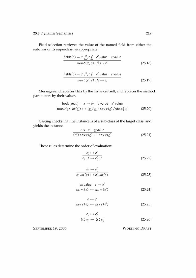
25.3 Dynamic Semantics 219
Field selection retrieves the value of the named field from either thesubclass or its superclass, as appropriate.
fields(c) = c′ f ′, c f e′ value e value
new c(e′, e). f ′i 7→ e′i (25.18)
fields(c) = c′ f ′, c f e′ value e value
new c(e′, e). fi 7→ ei (25.19)
Message send replaces this by the instance itself, and replaces the methodparameters by their values.
body(m, c) = x → e0 e value e′ value
new c(e).m(e′) 7→ e′/xnew c(e)/thise0 (25.20)
Casting checks that the instance is of a sub-class of the target class, andyields the instance.
c <: c′ e value
(c′) new c(e) 7→ new c(e) (25.21)
These rules determine the order of evaluation:
e0 7→ e′0e0. f 7→ e′0. f (25.22)
e0 7→ e′0e0.m(e) 7→ e′0.m(e) (25.23)
e0 value e 7→ e′
e0.m(e) 7→ e0.m(e′) (25.24)
e 7→ e′
new c(e) 7→ new c(e′) (25.25)
e0 7→ e′0(c) e0 7→ (c) e′0 (25.26)
SEPTEMBER 19, 2005 WORKING DRAFT
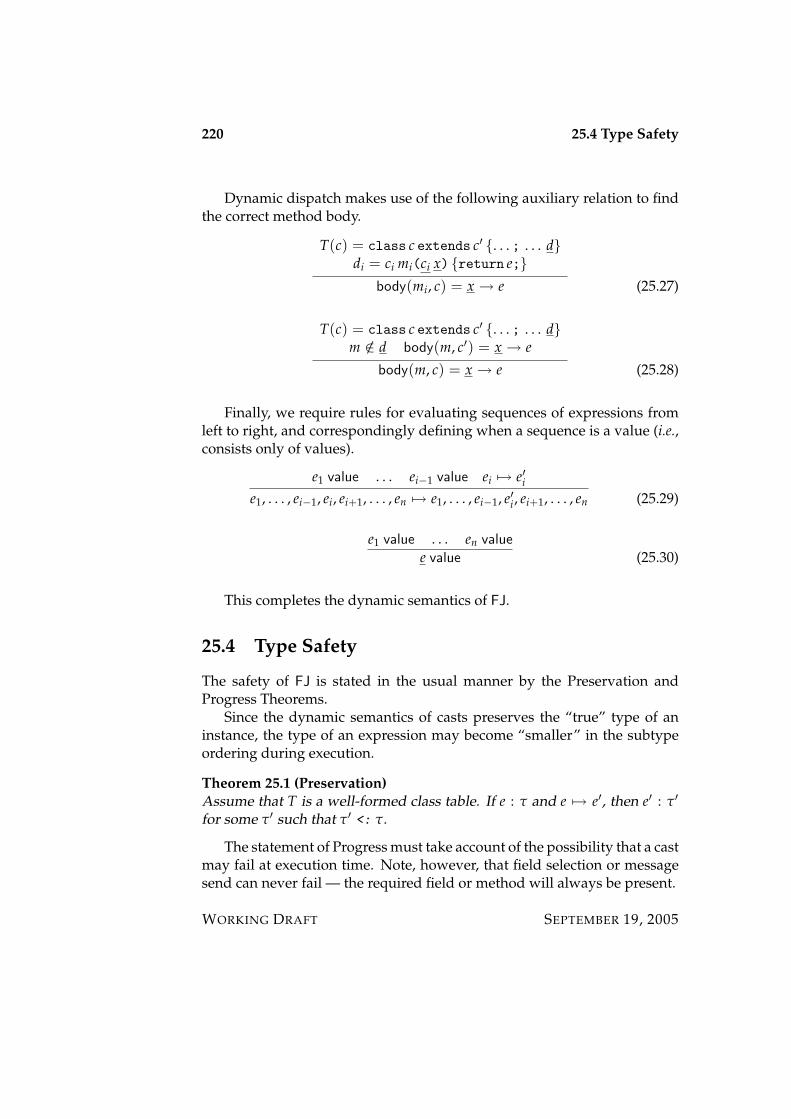
220 25.4 Type Safety
Dynamic dispatch makes use of the following auxiliary relation to findthe correct method body.
T(c) = class c extends c′ . . . ; . . . ddi = ci mi(ci x) return e;
body(mi, c) = x → e (25.27)
T(c) = class c extends c′ . . . ; . . . dm /∈ d body(m, c′) = x → e
body(m, c) = x → e (25.28)
Finally, we require rules for evaluating sequences of expressions fromleft to right, and correspondingly defining when a sequence is a value (i.e.,consists only of values).
e1 value . . . ei−1 value ei 7→ e′ie1, . . . , ei−1, ei, ei+1, . . . , en 7→ e1, . . . , ei−1, e′i, ei+1, . . . , en (25.29)
e1 value . . . en value
e value (25.30)
This completes the dynamic semantics of FJ.
25.4 Type Safety
The safety of FJ is stated in the usual manner by the Preservation andProgress Theorems.
Since the dynamic semantics of casts preserves the “true” type of aninstance, the type of an expression may become “smaller” in the subtypeordering during execution.
Theorem 25.1 (Preservation)Assume that T is a well-formed class table. If e : τ and e 7→ e′, then e′ : τ′
for some τ′ such that τ′ <: τ.
The statement of Progress must take account of the possibility that a castmay fail at execution time. Note, however, that field selection or messagesend can never fail — the required field or method will always be present.
WORKING DRAFT SEPTEMBER 19, 2005

25.5 Acknowledgement 221
Theorem 25.2 (Progress)Assume that T is a well-formed class table. If e : τ then either
1. v value, or
2. e contains an instruction of the form (c) new c′(e0) with e0 value andc′ 6<: c, or
3. there exists e′ such that e 7→ e′.
It follows that if no casts occur in the source program, then the secondcase cannot arise. This can be sharpened somewhat to admit source-levelcasts for which it is known statically that the type of casted expression is asubtype of the target of the cast. However, we cannot predict, in general,statically whether a given cast will succeed or fail dynamically.
Lemma 25.3 (Canonical Forms)If e : c and e value, then e has the form new c′(e0) with e0 value and c′ <: c.
25.5 Acknowledgement
This chapter is based on “Featherweight Java: A Minimal Core Calculusfor Java and GJ” by Atsushi Igarashi, Benjamin Pierce, and Philip Wadler.
SEPTEMBER 19, 2005 WORKING DRAFT

222 25.5 Acknowledgement
WORKING DRAFT SEPTEMBER 19, 2005

Part X
Subtyping and Inheritance
223

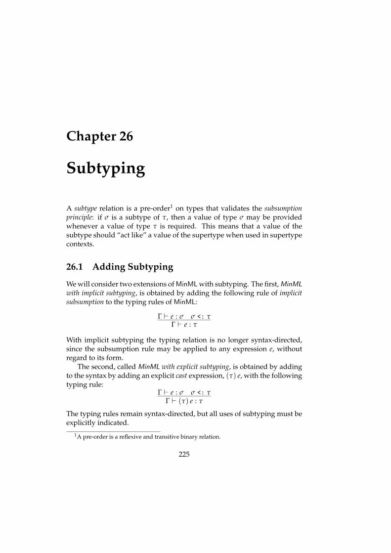
Chapter 26
Subtyping
A subtype relation is a pre-order1 on types that validates the subsumptionprinciple: if σ is a subtype of τ, then a value of type σ may be providedwhenever a value of type τ is required. This means that a value of thesubtype should “act like” a value of the supertype when used in supertypecontexts.
26.1 Adding Subtyping
We will consider two extensions of MinML with subtyping. The first, MinMLwith implicit subtyping, is obtained by adding the following rule of implicitsubsumption to the typing rules of MinML:
Γ ` e : σ σ <: τΓ ` e : τ
With implicit subtyping the typing relation is no longer syntax-directed,since the subsumption rule may be applied to any expression e, withoutregard to its form.
The second, called MinML with explicit subtyping, is obtained by addingto the syntax by adding an explicit cast expression, (τ) e, with the followingtyping rule:
Γ ` e : σ σ <: τΓ ` (τ) e : τ
The typing rules remain syntax-directed, but all uses of subtyping must beexplicitly indicated.
1A pre-order is a reflexive and transitive binary relation.
225
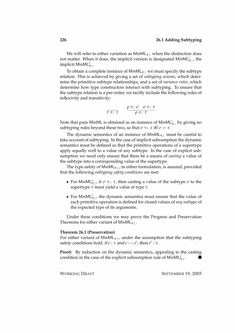
226 26.1 Adding Subtyping
We will refer to either variation as MinML<: when the distinction doesnot matter. When it does, the implicit version is designated MinMLi
<:, theimplicit MinMLe
<:.
To obtain a complete instance of MinML<: we must specify the subtyperelation. This is achieved by giving a set of subtyping axioms, which deter-mine the primitive subtype relationships, and a set of variance rules, whichdetermine how type constructors interact with subtyping. To ensure thatthe subtype relation is a pre-order, we tacitly include the following rules ofreflexivity and transitivity:
τ <: τρ <: σ σ <: τ
ρ <: τ
Note that pure MinML is obtained as an instance of MinMLi<: by giving no
subtyping rules beyond these two, so that σ <: τ iff σ = τ.
The dynamic semantics of an instance of MinML<: must be careful totake account of subtyping. In the case of implicit subsumption the dynamicsemantics must be defined so that the primitive operations of a supertypeapply equally well to a value of any subtype. In the case of explicit sub-sumption we need only ensure that there be a means of casting a value ofthe subtype into a corresponding value of the supertype.
The type safety of MinML<:, in either formulation, is assured, providedthat the following subtyping safety conditions are met:
• For MinMLe<:, if σ <: τ, then casting a value of the subtype σ to the
supertype τ must yield a value of type τ.
• For MinMLi<:, the dynamic semantics must ensure that the value of
each primitive operation is defined for closed values of any subtype ofthe expected type of its arguments.
Under these conditions we may prove the Progress and PreservationTheorems for either variant of MinML<:.
Theorem 26.1 (Preservation)For either variant of MinML<:, under the assumption that the subtypingsafety conditions hold, if e : τ and e 7→ e′, then e′ : τ.
Proof: By induction on the dynamic semantics, appealing to the castingcondition in the case of the explicit subsumption rule of MinMLe
<:.
WORKING DRAFT SEPTEMBER 19, 2005
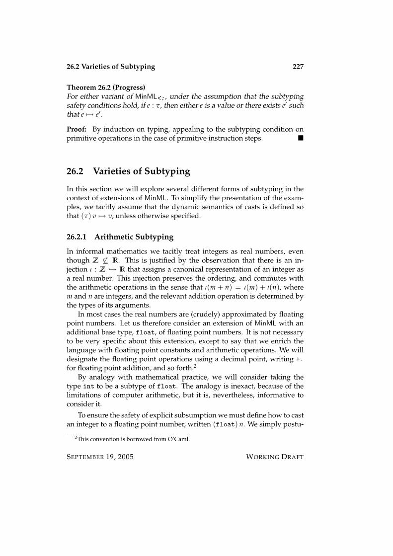
26.2 Varieties of Subtyping 227
Theorem 26.2 (Progress)For either variant of MinML<:, under the assumption that the subtypingsafety conditions hold, if e : τ, then either e is a value or there exists e′ suchthat e 7→ e′.
Proof: By induction on typing, appealing to the subtyping condition onprimitive operations in the case of primitive instruction steps.
26.2 Varieties of Subtyping
In this section we will explore several different forms of subtyping in thecontext of extensions of MinML. To simplify the presentation of the exam-ples, we tacitly assume that the dynamic semantics of casts is defined sothat (τ) v 7→ v, unless otherwise specified.
26.2.1 Arithmetic Subtyping
In informal mathematics we tacitly treat integers as real numbers, eventhough Z 6⊆ R. This is justified by the observation that there is an in-jection ι : Z → R that assigns a canonical representation of an integer asa real number. This injection preserves the ordering, and commutes withthe arithmetic operations in the sense that ι(m + n) = ι(m) + ι(n), wherem and n are integers, and the relevant addition operation is determined bythe types of its arguments.
In most cases the real numbers are (crudely) approximated by floatingpoint numbers. Let us therefore consider an extension of MinML with anadditional base type, float, of floating point numbers. It is not necessaryto be very specific about this extension, except to say that we enrich thelanguage with floating point constants and arithmetic operations. We willdesignate the floating point operations using a decimal point, writing +.for floating point addition, and so forth.2
By analogy with mathematical practice, we will consider taking thetype int to be a subtype of float. The analogy is inexact, because of thelimitations of computer arithmetic, but it is, nevertheless, informative toconsider it.
To ensure the safety of explicit subsumption we must define how to castan integer to a floating point number, written (float) n. We simply postu-
2This convention is borrowed from O’Caml.
SEPTEMBER 19, 2005 WORKING DRAFT
228 26.2 Varieties of Subtyping
late that this is possible, writing n.0 for the floating point representation ofthe integer n, and noting that n.0 has type float.3
To ensure the safety of implicit subsumption we must ensure that thefloating point arithmetic operations are well-defined for integer arguments.For example, we must ensure that an expression such as +.(3, 4) has a well-defined value as a floating point number. To achieve this, we simply requirethat floating point operations implicitly convert any integer arguments tofloating point before performing the operation. In the foregoing exampleevaluation proceeds as follows:
+.(3, 4) 7→ +.(3.0, 4.0) 7→ 7.0.
This strategy requires that the floating point operations detect the presenceof integer arguments, and that it convert any such arguments to floatingpoint before carrying out the operation. We will have more to say aboutthis inefficiency in Section 26.4 below.
26.2.2 Function Subtyping
Suppose that int <: float. What subtyping relationships, if any, shouldhold among the following four types?
1. int→int
2. int→float
3. float→int
4. float→float
To determine the answer, keep in mind the subsumption principle, whichsays that a value of the subtype should be usable in a supertype context.
Suppose f : int→int. If we apply f to x : int, the result has typeint, and hence, by the arithmetic subtyping axiom, has type float. Thissuggests that
int→int <: int→float
is a valid subtype relationship. By similar reasoning, we may derive that
float→int <: float→float
3We may handle the limitations of precision by allowing for a cast operation to fail inthe case of overflow. We will ignore overflow here, for the sake of simplicity.
WORKING DRAFT SEPTEMBER 19, 2005

26.2 Varieties of Subtyping 229
is also valid.Now suppose that f : float→int. If x : int, then x : float by sub-
sumption, and hence we may apply f to x to obtain a result of type int.This suggests that
float→int <: int→int
is a valid subtype relationship. Since int→int <: int→float, it followsthat
float→int <: int→float
is also valid.Subtyping rules that specify how a type constructor interacts with sub-
typing are called variance principles. If a type constructor preserves subtyp-ing in a given argument position, it is said to be covariant in that position. If,instead, it inverts subtyping in a given position it is said to be contravariantin that position. The discussion above suggests that the function space con-structor is covariant in the range position and contravariant in the domainposition. This is expressed by the following rule:
τ1 <: σ1 σ2 <: τ2σ1→σ2 <: τ1→τ2
Note well the inversion of subtyping in the domain, where the functionconstructor is contravariant, and the preservation of subtyping in the range,where the function constructor is covariant.
To ensure safety in the explicit case, we define the dynamic semanticsof a cast operation by the following rule:
(τ1→τ2) v 7→ fn x:τ1 in (τ2) v((σ1) x)
Here v has type σ1→σ2, τ1 <: σ1, and σ2 <: τ2. The argument is cast tothe domain type of the function prior to the call, and its result is cast to theintended type of the application.
To ensure safety in the implicit case, we must ensure that the primi-tive operation of function application behaves correctly on a function of asubtype of the “expected” type. This amounts to ensuring that a functioncan be called with an argument of, and yields a result of, a subtype of theintended type. One way is to adopt a semantics of procedure call that isindependent of the types of the arguments and results. Another is to intro-duce explicit run-time checks similar to those suggested for floating pointarithmetic to ensure that calling conventions for different types can be met.
SEPTEMBER 19, 2005 WORKING DRAFT
230 26.2 Varieties of Subtyping
26.2.3 Product and Record Subtyping
In Chapter 19 we considered an extension of MinML with product types.In this section we’ll consider equipping this extension with subtyping. Wewill work with n-ary products of the form τ1* · · · *τn and with n-ary recordsof the form l1:τ1, . . . ,ln:τn. The tuple types have as elements n-tuplesof the form <e1, . . . ,en> whose ith component is accessed by projection, e.i.Similarly, record types have as elements records of the form l1:e1, . . . ,ln:enwhose lth component is accessed by field selection, e.l.
Using the subsumption principle as a guide, it is natural to consider atuple type to be a subtype of any of its prefixes:
m > nτ1* · · · *τm <: τ1* · · · *τn
Given a value of type τ1* · · · *τn, we can access its ith component, for any1 ≤ i ≤ n. If m > n, then we can equally well access the ith componentof an m-tuple of type τ1* · · · *τm, obtaining the same result. This is calledwidth subtyping for tuples.
For records it is natural to consider a record type to be a subtype ofany record type with any subset of the fields of the subtype. This may bewritten as follows:
m > nl1:τ1, . . . ,lm:τm <: l1:τ1, . . . ,ln:τn
Bear in mind that the ordering of fields in a record type is immaterial, sothis rule allows us to neglect any subset of the fields when passing to asupertype. This is called width subtyping for records. The justification forwidth subtyping is that record components are accessed by label, ratherthan position, and hence the projection from a supertype value will applyequally well to the subtype.
What variance principles apply to tuples and records? Applying theprinciple of subsumption, it is easy to see that tuples and records may beregarded as covariant in all their components. That is,
∀1 ≤ i ≤ n σi <: τiσ1* · · · *σn <: τ1* · · · *τn
and∀1 ≤ i ≤ n σi <: τi
l1:σ1, . . . ,ln:σn <: l1:τ1, . . . ,ln:τn.
These are called depth subtyping rules for tuples and records, respectively.
WORKING DRAFT SEPTEMBER 19, 2005
26.2 Varieties of Subtyping 231
To ensure safety for explicit subsumption we must define the meaningof casting from a sub- to a super-type. The two forms of casting corre-sponding to width and depth subtyping may be consolidated into one, asfollows:
m ≥ n(τ1* · · · *τn) <v1, . . . ,vm> 7→ <(τ1) v1, . . . ,(τn) vn>.
An analogous rule defines the semantics of casting for record types.To ensure safety for implicit subsumption we must ensure that projec-
tion is well-defined on a subtype value. In the case of tuples this meansthat the operation of accessing the ith component from a tuple must be in-sensitive to the size of the tuple, beyond the basic requirement that it havesize at least i. This can be expressed schematically as follows:
<v1, . . . ,vi,. . .>.i 7→ vi.
The ellision indicates that fields beyond the ith are not relevant to the op-eration. Similarly, for records we postulate that selection of the lth field isinsensitive to the presence of any other fields:
l:v,. . ..l 7→ v.
The ellision expresses the independence of field selection from any “extra”fields.
26.2.4 Reference Subtyping
Finally, let us consider the reference types of Chapter 14. What should bethe variance rule for reference types? Suppose that r has type σ ref. Wecan do one of two things with r:
1. Retrieve its contents as a value of type σ.
2. Replace its contents with a value of type σ.
If σ <: τ, then retrieving the contents of r yields a value of type τ, bysubsumption. This suggests that references are covariant:
σ <: τ
σ ref?<: τ ref.
SEPTEMBER 19, 2005 WORKING DRAFT
232 26.3 Type Checking With Subtyping
On the other hand, if τ <: σ, then we may store a value of type τ into r.This suggests that references are contravariant:
τ <: σ
σ ref?<: τ ref.
Given that we may perform either operation on a reference cell, wemust insist that reference types are invariant:
σ <: τ τ <: σσ ref <: τ ref .
The premise of the rule is often strengthened to the requirement that σ andτ be equal:
σ = τσ ref <: τ ref
since there are seldom situations where distinct types are mutual subtypes.A similar analysis may be applied to any mutable data structure. For
example, immutable sequences may be safely taken to be covariant, but mu-table sequences (arrays) must be taken to be invariant, lest safety be com-promised.
26.3 Type Checking With Subtyping
Type checking for MinML<:, in either variant, clearly requires an algorithmfor deciding subtyping: given σ and τ, determine whether or not σ <:τ. The difficulty of deciding type checking is dependent on the specificrules under consideration. In this section we will discuss type checking forMinML<:, under the assumption that we can check the subtype relation.
Consider first the explicit variant of MinML<:. Since the typing rulesare syntax directed, we can proceed as for MinML, with one additional caseto consider. To check whether (σ) e has type τ, we must check two things:
1. Whether e has type σ.
2. Whether σ <: τ.
The former is handled by a recursive call to the type checker, the latter bya call to the subtype checker, which we assume given.
This discussion glosses over an important point. Even in pure MinMLit is not possible to determine directly whether or not Γ ` e : τ. For sup-pose that e is an application e1(e2). To check whether Γ ` e : τ, we must
WORKING DRAFT SEPTEMBER 19, 2005
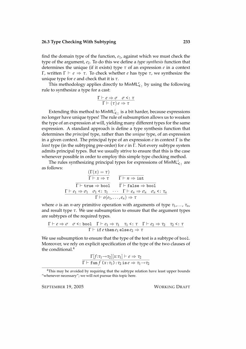
26.3 Type Checking With Subtyping 233
find the domain type of the function, e1, against which we must check thetype of the argument, e2. To do this we define a type synthesis function thatdetermines the unique (if it exists) type τ of an expression e in a contextΓ, written Γ ` e ⇒ τ. To check whether e has type τ, we synthesize theunique type for e and check that it is τ.
This methodology applies directly to MinMLe<: by using the following
rule to synthesize a type for a cast:
Γ ` e⇒ σ σ <: τΓ ` (τ) e⇒ τ
Extending this method to MinMLi<: is a bit harder, because expressions
no longer have unique types! The rule of subsumption allows us to weakenthe type of an expression at will, yielding many different types for the sameexpression. A standard approach is define a type synthesis function thatdetermines the principal type, rather than the unique type, of an expressionin a given context. The principal type of an expression e in context Γ is theleast type (in the subtyping pre-order) for e in Γ. Not every subtype systemadmits principal types. But we usually strive to ensure that this is the casewhenever possible in order to employ this simple type checking method.
The rules synthesizing principal types for expressions of MinMLi<: are
as follows:(Γ(x) = τ)Γ ` x ⇒ τ Γ ` n⇒ int
Γ ` true⇒ bool Γ ` false⇒ boolΓ ` e1 ⇒ σ1 σ1 <: τ1 · · · Γ ` en ⇒ σn σn <: τn
Γ ` o(e1, . . . , en)⇒ τ
where o is an n-ary primitive operation with arguments of type τ1,. . . , τn,and result type τ. We use subsumption to ensure that the argument typesare subtypes of the required types.
Γ ` e⇒ σ σ <: bool Γ ` e1 ⇒ τ1 τ1 <: τ Γ ` e2 ⇒ τ2 τ2 <: τ
Γ ` if e then e1 else e2 ⇒ τ
We use subsumption to ensure that the type of the test is a subtype of bool.Moreover, we rely on explicit specification of the type of the two clauses ofthe conditional.4
Γ[ f :τ1→τ2][x:τ1] ` e⇒ τ2
Γ ` fun f (x:τ1):τ2 is e⇒ τ1→τ2
4This may be avoided by requiring that the subtype relation have least upper bounds“whenever necessary”; we will not pursue this topic here.
SEPTEMBER 19, 2005 WORKING DRAFT
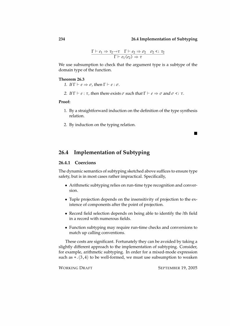
234 26.4 Implementation of Subtyping
Γ ` e1 ⇒ τ2→τ Γ ` e2 ⇒ σ2 σ2 <: τ2
Γ ` e1(e2)⇒ τ
We use subsumption to check that the argument type is a subtype of thedomain type of the function.
Theorem 26.31. If Γ ` e⇒ σ, then Γ ` e : σ.
2. If Γ ` e : τ, then there exists σ such that Γ ` e⇒ σ and σ <: τ.
Proof:
1. By a straightforward induction on the definition of the type synthesisrelation.
2. By induction on the typing relation.
26.4 Implementation of Subtyping
26.4.1 Coercions
The dynamic semantics of subtyping sketched above suffices to ensure typesafety, but is in most cases rather impractical. Specifically,
• Arithmetic subtyping relies on run-time type recognition and conver-sion.
• Tuple projection depends on the insensitivity of projection to the ex-istence of components after the point of projection.
• Record field selection depends on being able to identify the lth fieldin a record with numerous fields.
• Function subtyping may require run-time checks and conversions tomatch up calling conventions.
These costs are significant. Fortunately they can be avoided by taking aslightly different approach to the implementation of subtyping. Consider,for example, arithmetic subtyping. In order for a mixed-mode expressionsuch as +.(3,4) to be well-formed, we must use subsumption to weaken
WORKING DRAFT SEPTEMBER 19, 2005
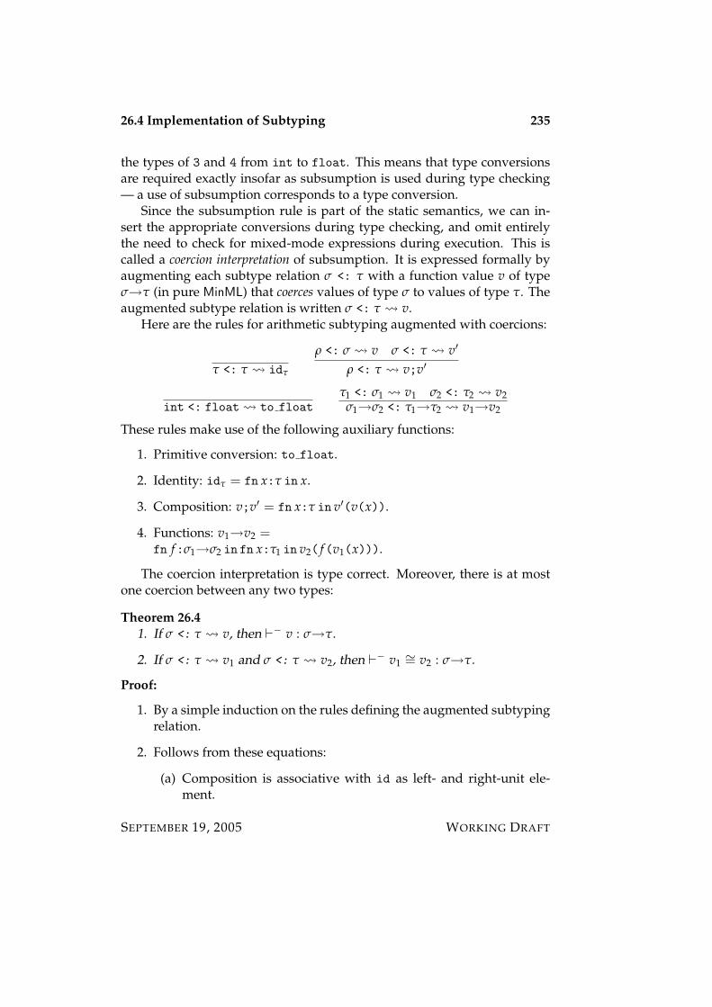
26.4 Implementation of Subtyping 235
the types of 3 and 4 from int to float. This means that type conversionsare required exactly insofar as subsumption is used during type checking— a use of subsumption corresponds to a type conversion.
Since the subsumption rule is part of the static semantics, we can in-sert the appropriate conversions during type checking, and omit entirelythe need to check for mixed-mode expressions during execution. This iscalled a coercion interpretation of subsumption. It is expressed formally byaugmenting each subtype relation σ <: τ with a function value v of typeσ→τ (in pure MinML) that coerces values of type σ to values of type τ. Theaugmented subtype relation is written σ <: τ v.
Here are the rules for arithmetic subtyping augmented with coercions:
τ <: τ idτ
ρ <: σ v σ <: τ v′
ρ <: τ v;v′
int <: float to floatτ1 <: σ1 v1 σ2 <: τ2 v2
σ1→σ2 <: τ1→τ2 v1→v2
These rules make use of the following auxiliary functions:
1. Primitive conversion: to float.
2. Identity: idτ = fn x:τ in x.
3. Composition: v;v′ = fn x:τ in v′(v(x)).
4. Functions: v1→v2 =fn f:σ1→σ2 in fn x:τ1 in v2( f(v1(x))).
The coercion interpretation is type correct. Moreover, there is at mostone coercion between any two types:
Theorem 26.41. If σ <: τ v, then `− v : σ→τ.
2. If σ <: τ v1 and σ <: τ v2, then `− v1∼= v2 : σ→τ.
Proof:
1. By a simple induction on the rules defining the augmented subtypingrelation.
2. Follows from these equations:
(a) Composition is associative with id as left- and right-unit ele-ment.
SEPTEMBER 19, 2005 WORKING DRAFT
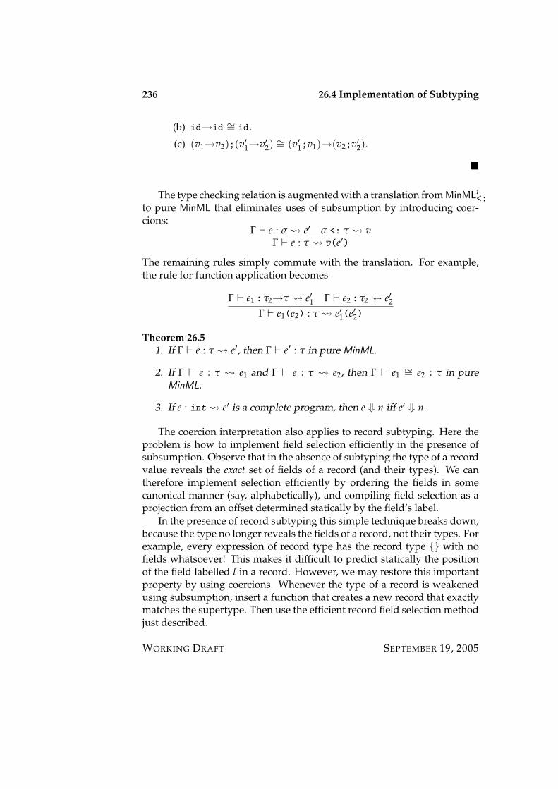
236 26.4 Implementation of Subtyping
(b) id→id ∼= id.
(c) (v1→v2);(v′1→v′2) ∼= (v′1;v1)→(v2;v′2).
The type checking relation is augmented with a translation from MinMLi<:
to pure MinML that eliminates uses of subsumption by introducing coer-cions:
Γ ` e : σ e′ σ <: τ vΓ ` e : τ v(e′)
The remaining rules simply commute with the translation. For example,the rule for function application becomes
Γ ` e1 : τ2→τ e′1 Γ ` e2 : τ2 e′2Γ ` e1(e2) : τ e′1(e′2)
Theorem 26.51. If Γ ` e : τ e′, then Γ ` e′ : τ in pure MinML.
2. If Γ ` e : τ e1 and Γ ` e : τ e2, then Γ ` e1∼= e2 : τ in pure
MinML.
3. If e : int e′ is a complete program, then e ⇓ n iff e′ ⇓ n.
The coercion interpretation also applies to record subtyping. Here theproblem is how to implement field selection efficiently in the presence ofsubsumption. Observe that in the absence of subtyping the type of a recordvalue reveals the exact set of fields of a record (and their types). We cantherefore implement selection efficiently by ordering the fields in somecanonical manner (say, alphabetically), and compiling field selection as aprojection from an offset determined statically by the field’s label.
In the presence of record subtyping this simple technique breaks down,because the type no longer reveals the fields of a record, not their types. Forexample, every expression of record type has the record type with nofields whatsoever! This makes it difficult to predict statically the positionof the field labelled l in a record. However, we may restore this importantproperty by using coercions. Whenever the type of a record is weakenedusing subsumption, insert a function that creates a new record that exactlymatches the supertype. Then use the efficient record field selection methodjust described.
WORKING DRAFT SEPTEMBER 19, 2005
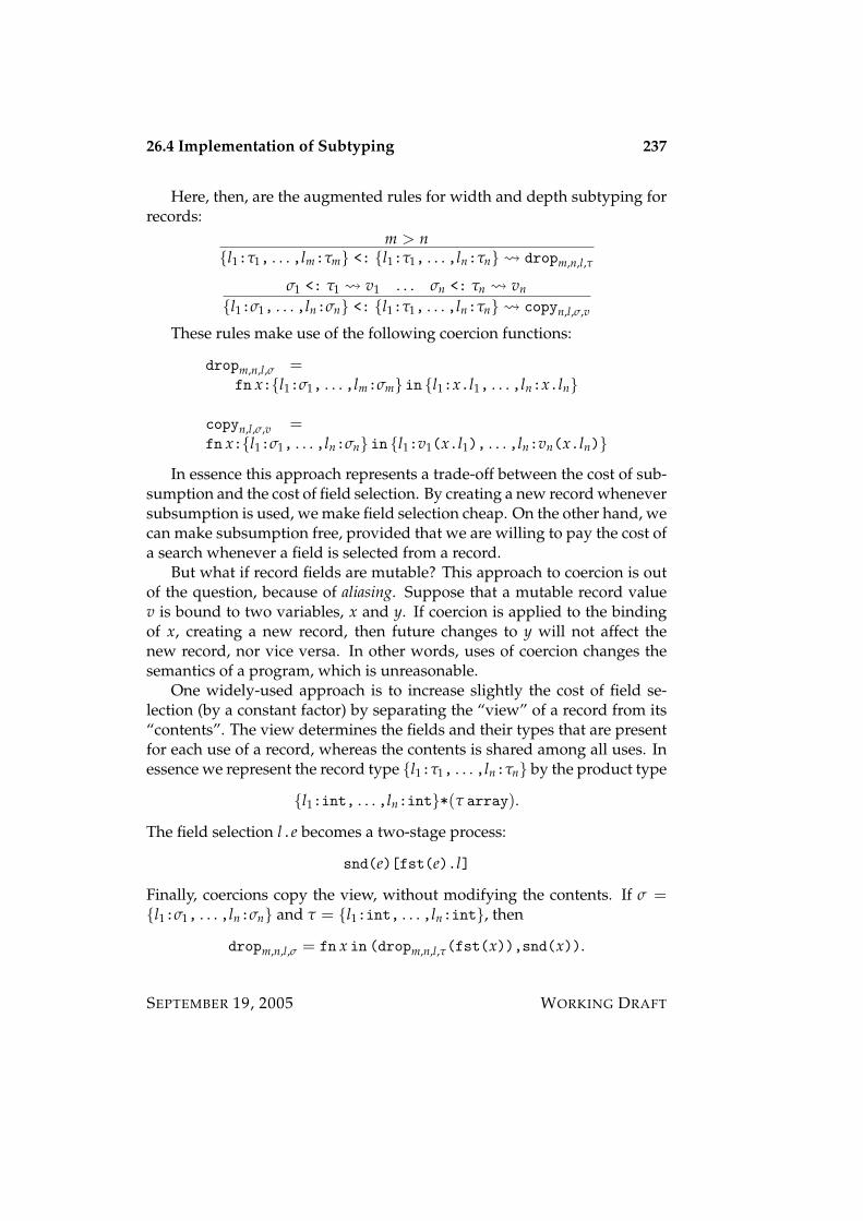
26.4 Implementation of Subtyping 237
Here, then, are the augmented rules for width and depth subtyping forrecords:
m > nl1:τ1, . . . ,lm:τm <: l1:τ1, . . . ,ln:τn dropm,n,l,τ
σ1 <: τ1 v1 . . . σn <: τn vn
l1:σ1, . . . ,ln:σn <: l1:τ1, . . . ,ln:τn copyn,l,σ,v
These rules make use of the following coercion functions:
dropm,n,l,σ =fn x:l1:σ1, . . . ,lm:σm in l1:x.l1, . . . ,ln:x.ln
copyn,l,σ,v =fn x:l1:σ1, . . . ,ln:σn in l1:v1(x.l1), . . . ,ln:vn(x.ln)
In essence this approach represents a trade-off between the cost of sub-sumption and the cost of field selection. By creating a new record wheneversubsumption is used, we make field selection cheap. On the other hand, wecan make subsumption free, provided that we are willing to pay the cost ofa search whenever a field is selected from a record.
But what if record fields are mutable? This approach to coercion is outof the question, because of aliasing. Suppose that a mutable record valuev is bound to two variables, x and y. If coercion is applied to the bindingof x, creating a new record, then future changes to y will not affect thenew record, nor vice versa. In other words, uses of coercion changes thesemantics of a program, which is unreasonable.
One widely-used approach is to increase slightly the cost of field se-lection (by a constant factor) by separating the “view” of a record from its“contents”. The view determines the fields and their types that are presentfor each use of a record, whereas the contents is shared among all uses. Inessence we represent the record type l1:τ1, . . . ,ln:τn by the product type
l1:int, . . . ,ln:int*(τ array).
The field selection l.e becomes a two-stage process:
snd(e)[fst(e).l]
Finally, coercions copy the view, without modifying the contents. If σ =l1:σ1, . . . ,ln:σn and τ = l1:int, . . . ,ln:int, then
dropm,n,l,σ = fn x in (dropm,n,l,τ(fst(x)),snd(x)).
SEPTEMBER 19, 2005 WORKING DRAFT
238 26.4 Implementation of Subtyping
WORKING DRAFT SEPTEMBER 19, 2005
Chapter 27
Inheritance and Subtyping inJava
In this note we discuss the closely-related, but conceptually distinct, no-tions of inheritance, or subclassing, and subtyping as exemplified in the Javalanguage. Inheritance is a mechanism for supporting code re-use throughincremental extension and modification. Subtyping is a mechanism for ex-pressing behavioral relationships between types that allow values of a sub-type to be provided whenever a value of a supertype is required.
In Java inheritance relationships give rise to subtype relationships, butnot every subtype relationship arises via inheritance. Moreover, there arelanguages (including some extensions of Java) for which subclasses do notgive rise to subtypes, and there are languages with no classes at all, butwith a rich notion of subtyping. For these reasons it is best to keep a cleardistinction between subclassing and subtyping.
27.1 Inheritance Mechanisms in Java
27.1.1 Classes and Instances
The fundamental unit of inheritance in Java is the class. A class consistsof a collection of fields and a collection of methods. Fields are assignablevariables; methods are procedures acting on these variables. Fields andmethods can be either static (per-class) or dynamic (per-instance).1 Staticfields are per-class data. Static methods are just ordinary functions actingon static fields.
1Fields and methods are assumed dynamic unless explicitly declared to be static.
239

240 27.1 Inheritance Mechanisms in Java
Classes give rise to instances, or objects, that consist of the dynamic meth-ods of the class together with fresh copies (or instances) of its dynamicfields. Instances of classes are created by a constructor, whose role is to allo-cate and initialize fresh copies of the dynamic fields (which are also knownas instance variables). Constructors have the same name as their class, andare invoked by writing new C(e1, . . . , en), where C is a class and e1, . . . , enare arguments to the constructor.2 Static methods have access only to thestatic fields (and methods) of its class; dynamic methods have access toboth the static and dynamic fields and methods of the class.
The components of a class have a designated visibility attribute, eitherpublic, private, or protected. The public components are those that areaccessible by all clients of the class. Public static components are accessi-ble to any client with access to the class. Public dynamic components arevisible to any client of any instance of the class. Protected components are“semi-private; we’ll have more to say about protected components later.
The components of a class also have a finality attribute. Final fields arenot assignable — they are read-only attributes of the class or instance. Ac-tually, final dynamic fields can be assigned exactly once, by a constructorof the class, to initialize their values. Final methods are of interest in con-nection with inheritance, to which we’ll return below.
The components of a class have types. The type of a field is the type of itsbinding as a (possibly assignable) variable. The type of a method specifiesthe types of its arguments (if any) and the type of its results. The type of aconstructor specifies the types of its arguments (if any); its “result type” isthe instance type of the class itself, and may not be specified explicitly. (Wewill say more about the type structure of Java below.)
The public static fields and methods of a class C are accessed using“dot notation”. If f is a static field of C, a client may refer to it by writ-ing C. f . Similarly, if m is a static method of C, a client may invoke it bywriting C.m(e1,...,en), where e1, . . . , en are the argument expressions ofthe method. The expected type checking rules govern access to fields andinvocations of methods.
The public dynamic fields and methods of an instance c of a class Care similarly accessed using “dot notation”, albeit from the instance, ratherthan the class. That is, if f is a public dynamic field of C, then c. f refersto the f field of the instance c. Since distinct instances have distinct fields,there is no essential connection between c. f and c′. f when c and c′ are
2Classes can have multiple constructors that are distinguished by overloading. We willnot discuss overloading here.
WORKING DRAFT SEPTEMBER 19, 2005
27.1 Inheritance Mechanisms in Java 241
distinct instances of class C. If m is a public dynamic method of C, thenc.m(e1, . . . , en) invokes the method m of the instance c with the specifiedarguments. This is sometimes called sending a message m to instance c witharguments e1, . . . , en.
Within a dynamic method one may refer to the dynamic fields andmethods of the class via the pseudo-variable this, which is bound to theinstance itself. The methods of an instance may call one another (or them-selves) by sending a message to this. Although Java defines conventionswhereby explicit reference to this may be omitted, it is useful to eschewthese conveniences and always use this to refer to the components of aninstance from within code for that instance. We may think of this as animplicit argument to all methods that allows the method to access to objectitself.
27.1.2 Subclasses
A class may be defined by inheriting the visible fields and methods of an-other class. The new class is said to be a subclass of the old class, the su-perclass. Consequently, inheritance is sometimes known as subclassing. Javasupports single inheritance — every class has at most one superclass. Thatis, one can only inherit from a single class; one cannot combine two classesby inheritance to form a third. In Java the subclass is said to extend thesuperclass.
There are two forms of inheritance available in Java:
1. Enrichment. The subclass enriches the superclass by providing addi-tional fields and methods not present in the superclass.
2. Overriding. The subclass may re-define a method in the superclass bygiving it a new implementation in the subclass.
Enrichment is a relatively innocuous aspect of inheritance. The true powerof inheritance lies in the ability to override methods.
Overriding, which is also known as method specialization, is used to “spe-cialize” the implementation of a superclass method to suit the needs of thesubclass. This is particularly important when the other methods of the classinvoke the overridden method by sending a message to this. If a methodm is overridden in a subclass D of a class C, then all methods of D thatinvoke m via this will refer to the “new” version of m defined by the over-ride. The “old” version can still be accessed explicitly from the subclass by
SEPTEMBER 19, 2005 WORKING DRAFT
242 27.1 Inheritance Mechanisms in Java
referring to super.m. The keyword super is a pseudo-variable that may beused to refer to the overridden methods.
Inheritance can be controlled using visibility constraints. A sub-classD of a class C automatically inherits the private fields and methods of Cwithout the possibility of overriding, or otherwise accessing, them. Thepublic fields and methods of the superclass are accessible to the subclasswithout restriction, and retain their public attribute in the subclass, unlessoverridden. A protected component is “semi-private” — accessible to thesubclass, but not otherwise publically visible.3
Inheritance can also be limited using finality constraints. If a methodis declared final, it may not be overridden in any subclass — it must beinherited as-is, without further modification. However, if a final methodinvokes, via this, a non-final method, then the behavior of the final methodcan still be changed by the sub-class by overriding the non-final method.By declaring an entire class to be final, no class can inherit from it. Thisserves to ensure that any instance of this class invokes the code from thisclass, and not from any subclass of it.
Instantiation of a subclass of a class proceeds in three phases:
1. The instance variables of the subclass, which include those of the su-perclass, are allocated.
2. The constructor of the superclass is invoked to initialize the super-class’s instance variables.
3. The constructor of the subclass is invoked to initialize the subclass’sinstance variables.
The superclass constructor can be explicitly invoked by a subclass construc-tor by writing super(e1, . . . , en), but only as the very first statement of thesubclass’s constructor. This ensures proper initialization order, and avoidscertain anomalies and insecurities that arise if this restriction is relaxed.
27.1.3 Abstract Classes and Interfaces
An abstract class is a class in which one or more methods are declared,but left unimplemented. Abstract methods may be invoked by the othermethods of an abstract class by sending a message to this, but since theirimplementation is not provided, abstract classes do not themselves have
3Actually, Java assigns protected components “package scope”, but since we are notdiscussing packages here, we will ignore this issue.
WORKING DRAFT SEPTEMBER 19, 2005
27.1 Inheritance Mechanisms in Java 243
instances. Instead the obligation is imposed on a subclass of the abstractclass to provide implementations of the abstract methods to obtain a con-crete class, which does have instances. Abstract classes are useful for settingup “code templates” that are instantiated by inheritance. The abstract classbecomes the locus of code sharing for all concretions of that class, whichinherit the shared code and provide the missing non-shared code.
Taking this idea to the extreme, an interface is a “fully abstract” class,which is to say that
• All its fields are public static final (i.e., they are constants).
• All its methods are abstract public; they must be implemented bya subclass.
Since interfaces are a special form of abstract class, they have no instances.The utility of interfaces stems from their role in implements declara-
tions. As we mentioned above, a class may be declared to extend a singleclass to inherit from it.4 A class may also be declared to implement one ormore interfaces, meaning that the class provides the public methods of theinterface, with their specified types. Since interfaces are special kinds ofclasses, Java is sometimes said to provide multiple inheritance of interfaces,but only single inheritance of implementation. For similar reasons an inter-face may be declared to extend multiple interfaces, provided that the resulttypes of their common methods coincide.
The purpose of declaring an interface for a class is to support writinggeneric code that works with any instance providing the methods specifiedin the interface, without requiring that instance to arise from any particularposition in the inheritance hierarchy. For example, we may have two un-related classes in the class hierarchy providing a method m. If both classesare declared to implement an interface that mentions m, then code pro-grammed against this interface will work for an instance of either class.
The literature on Java emphasizes that interfaces are descriptive of be-havior (to the extend that types alone allow), whereas classes are prescrip-tive of implementation. While this is surely a noble purpose, it is curiousthat interfaces are classes in Java, rather than types. In particular interfacesare unable to specify the public fields of an instance by simply stating theirtypes, which would be natural were interfaces a form of type. Instead fieldsin interfaces are forced to be constants (public, static, final), precluding theiruse for describing the public instance variables of an object.
4Classes that do not specify a superclass implicitly extend the class Object of all objects.
SEPTEMBER 19, 2005 WORKING DRAFT
244 27.2 Subtyping in Java
27.2 Subtyping in Java
The Java type system consists of the following types:
1. Base types, including int, float, void, and boolean.
2. Class types C, which classify the instances of a class C.
3. Array types of the form τ [ ], where τ is a type, representing mutablearrays of values of type τ.
The basic types behave essentially as one would expect, based on pre-vious experience with languages such as C and C++. Unlike C or C++ Javahas true array types, with operations for creating and initializing an arrayand for accessing and assigning elements of an array. All array operationsare safe in the sense that any attempt to exceed the bounds of the arrayresults in a checked error at run-time.
Every class, whether abstract or concrete, including interfaces, has as-sociated with it the type of its instances, called (oddly enough) the instancetype of the class. Java blurs the distinction between the class as a programstructure and the instance type determined by the class — class namesserve not only to identify the class but also the instance type of that class. Itmay seem odd that abstract classes, and interfaces, all define instance types,even though they don’t have instances. However, as will become clear be-low, even abstract classes have instances, indirectly through their concretesubclasses. Similarly, interfaces may be thought of as possessing instances,namely the instances of concrete classes that implement that interface.
27.2.1 Subtyping
To define the Java subtype relation we need two auxiliary relations. Thesubclass relation, C C C′, is the reflexive and transitive closure of the extendsrelation among classes, which holds precisely when one class is declared toextend another. In other words, C C C′ iff C either coincides with C′, in-herits directly from C′, or inherits from a subclass of C′. Since interfaces areclasses, the subclass relation also applies to interfaces, but note that multi-ple inheritance of interfaces means that an interface can be a subinterface(subclass) of more than one interface. The implementation relation, C J I, isdefined to hold exactly when a class C is declared to implement an interfacethat inherits from I.
WORKING DRAFT SEPTEMBER 19, 2005
27.2 Subtyping in Java 245
The Java subtype relation is inductively defined by the following rules.Subtyping is reflexive and transitive:
τ <: τ (27.1)
τ <: τ′ τ′ <: τ′′
τ <: τ′′ (27.2)
Arrays are covariant type constructors, in the sense of this rule:
τ <: τ′
τ [ ] <: τ′ [ ] (27.3)
Inheritance implies subtyping:
C C C′
C <: C′ (27.4)
Implementation implies subtyping:
C J IC <: I (27.5)
Every class is a subclass of the distinguished “root” class Object:
τ <: Object (27.6)
The array subtyping rule is a structural subtyping principle — one neednot explicitly declare subtyping relationships between array types for themto hold. On the other hand, the inheritance and implementation rules ofsubtyping are examples of nominal subtyping — they hold when they aredeclared to hold at the point of definition (or are implied by further sub-typing relations).
27.2.2 Subsumption
The subsumption principle tells us that if e is an expression of type τ andτ <: τ′, then e is also an expression of type τ′. In particular, if a methodis declared with a parameter of type τ, then it makes sense to provide anargument of any type τ′ such that τ′ <: τ. Similarly, if a constructor takesa parameter of a type, then it is legitimate to provide an argument of asubtype of that type. Finally, if a method is declared to return a value oftype τ, then it is legitimate to return a value of any subtype of τ.
SEPTEMBER 19, 2005 WORKING DRAFT
246 27.2 Subtyping in Java
This brings up an awkward issue in the Java type system. What shouldbe the type of a conditional expression e ? e1: e2? Clearly e should have typeboolean, and e1 and e2 should have the same type, since we cannot in gen-eral predict the outcome of the condition e. In the presence of subtyping,this amounts to the requirement that the types of e1 and e2 have an up-per bound in the subtype ordering. To avoid assigning an excessively weaktype, and to ensure that there is a unique choice of type for the conditional,it would make sense to assign the conditional the least upper bound of thetypes of e1 and e2. Unfortunately, two types need not have a least upperbound! For example, if an interface I extends incomparable interfaces Kand L, and J extends both K and L, then I and J do not have a least upperbound — both K and L are upper bounds of both, but neither is smallerthan the other. To deal with this Java imposes the rather ad hoc requirementthat either the type of e1 be a subtype of the type of e2, or vice versa, to avoidthe difficulty.
A more serious difficulty with the Java type system is that the array sub-typing rule, which states that the array type constructor is covariant in thetype of the array elements, violates the subsumption principle. To under-stand why, recall that we can do one of two things with an array: retrievean element, or assign to an element. If τ <: τ′ and A is an array of typeτ [ ], then retrieving an element of A yields a value of type τ, which is byhypothesis an element of type τ′. So we are OK with respect to retrieval.Now consider array assignment. Suppose once again that τ <: τ′ and thatA is an array of type τ [ ]. Then A is also an array of type τ′ [ ], accordingto the Java rule for array subtyping. This means we can assign a value xof type τ′ to an element of A. But this violates the assumption that A is anarray of type τ [ ] — one of its elements is of type τ′.
With no further provisions the language would not be type safe. It isa simple matter to contrive an example involving arrays that incurs a run-time type error (“gets stuck”). Java avoids this by a simple, but expensive,device — every array assignment incurs a “run-time type check” that en-sures that the assignment does not create an unsafe situation. In the nextsubsection we explain how this is achieved.
27.2.3 Dynamic Dispatch
According to Java typing rules, if C is a sub-class of D, then C is a sub-typeof D. Since the instances of a class C have type C, they also, by subsump-tion, have type D, as do the instances of class D itself. In other words, ifthe static type of an instance is D, it might be an instance of class C or an
WORKING DRAFT SEPTEMBER 19, 2005
27.2 Subtyping in Java 247
instance of class D. In this sense the static type of an instance is at best anapproximation of its dynamic type, the class of which it is an instance.
The distinction between the static and the dynamic type of an object isfundamental to object-oriented programming. In particular method spe-cialization is based on the dynamic type of an object, not its static type.Specifically, if C is a sub-class of D that overrides a method m, then invok-ing the method m of a C instance o will always refer to the overriding codein C, even if the static type of o is D. That is, method dispatch is basedon the dynamic type of the instance, not on its static type. For this reasonmethod specialization is sometimes called dynamic dispatch, or, less perspic-uously, late binding.
How is this achieved? Essentially, every object is tagged with the classthat created it, and this tag is used to determine which method to invokewhen a message is sent to that object. The constructors of a class C “label”the objects they create with C. The method dispatch mechanism consultsthis label when determining which method to invoke.5
The same mechanism is used to ensure that array assignments do notlead to type insecurities. Suppose that the static type of A is C [ ], andthat the static type of instance o is C. By covariance of array types thedynamic type of A might be D [ ] for some sub-class D of C. But unless thedynamic type of o is also D, the assignment of o to an element of A shouldbe prohibited. This is ensured by an explicit run-time check. In Java everysingle array assignment incurs a run-time check whenever the array containsobjects.6
27.2.4 Casting
A container class is one whose instances “contain” instances of another class.For example, a class of lists or trees or sets would be a container class inthis sense. Since the operations on containers are largely (or entirely) inde-pendent of the type of their elements, it makes sense to define containersgenerally, rather than defining one for each element type. In Java this isachieved by exploiting subsumption. Since every object has type Object,a general container is essentially a container whose elements are of typeObject. This allows the container operations to be defined once for all el-
5In practice the label is a pointer to the vector of methods of the class, and the method isaccessed by indexing into this vector. But we can just as easily imagine this to be achievedby a case analysis on the class name to determine the appropriate method vector.
6Arrays of integers and floats do not incur this overhead, because numbers are not ob-jects.
SEPTEMBER 19, 2005 WORKING DRAFT
248 27.2 Subtyping in Java
ement types. However, when retrieving an element from a container itsstatic type is Object; we lost track of its dynamic type during type check-ing. If we wish to use such an object in any meaningful way, we mustrecover its dynamic type so that message sends are not rejected at compiletime.
Java supports a safe form of casting, or change of type. A cast is written(τ) e. The expression e is called the subject of the cast, and the type τ is thetarget type of the cast. The type of the cast is τ, provided that the cast makessense, and its value is that of e. In general we cannot determine whetherthe cast makes sense until execution time, when the dynamic type of theexpression is available for comparison with the target type. For example,every instance in Java has type Object, but its true type will usually besome class further down the type hierarchy. Therefore a cast applied to anexpression of type Object cannot be validated until execution time.
Since the static type is an attenuated version of the dynamic type of anobject, we can classify casts into three varieties:
1. Up casts, in which the static type of the expression is a subtype ofthe target type of the cast. The type checker accepts the cast, and norun-time check is required.
2. Down casts, in which the static type of the expression is a supertype ofthe target type. The true type may or may not be a subtype of thetarget, so a run-time check is required.
3. Stupid casts, in which the static type of the expression rules out thepossibility of its dynamic type matching the target of the cast. Thecast is rejected.
Similar checks are performed to ensure that array assignments are safe.Note that it is up to the programmer to maintain a sufficiently strong
invariant to ensure that down casts do not fail. For example, if a containeris intended to contain objects of a class C, then retrieved elements of thatclass will typically be down cast to a sub-class of C. It is entirely up to theprogrammer to ensure that these casts do not fail at execution time. Thatis, the programmer must maintain the invariant that the retrieved elementreally contains an instance of the target class of the cast.
WORKING DRAFT SEPTEMBER 19, 2005

27.3 Methodology 249
27.3 Methodology
With this in hand we can (briefly) discuss the methodology of inheritancein object-oriented languages. As we just noted, in Java subclassing entailssubtyping — the instance type of a subclass is a subtype of the instance typeof the superclass. It is important to recognize that this is a methodologicalcommitment to certain uses of inheritance.
Recall that a subtype relationship is intended to express a form of be-havioral equivalence. This is expressed by the subsumption principle, whichstates that subtype values may be provided whenever a supertype value isrequired. In terms of a class hierarchy this means that a value of the sub-class can be provided whenever a value of the superclass is required. Forthis to make good sense the values of the subclass should “behave prop-erly” in superclass contexts — they should not be distinguishable fromthem.
But this isn’t necessarily so! Since inheritance admits overriding ofmethods, we can make almost arbitrary7 changes to the behavior of thesuperclass when defining the subclass. For example, we can turn a stack-like object into a queue-like object (replacing a LIFO discipline by a FIFOdiscipline) by inheritance, thereby changing the behavior drastically. If weare to pass off a subclass instance as a superclass instance using subtyping,then we should refrain from making such drastic behavioral changes.
The Java type system provides only weak tools for ensuring a behav-ioral subtyping relationship between a subclass and its superclass. Fun-damentally, the type system is not strong enough to express the desiredconstraints.8. To compensate for this Java provides the finality mechanismto limit inheritance. Final classes cannot be inherited from at all, ensuringthat values of its instance type are indeed instances of that class (rather thanan arbitrary subclass). Final methods cannot be overridden, ensuring thatcertain aspects of behavior are “frozen” by the class definition.
Nominal subtyping may also be seen as a tool for enforcing behavioralsubtyping relationships. For unless a class extends a given class or is de-clared to implement a given interface, no subtyping relationship holds.This helps to ensure that the programmer explicitly considers the behav-ioral subtyping obligations that are implied by such declarations, and istherefore an aid to controlling inheritance.
7Limited only by finality declarations in the superclass.8Nor is the type system of any other language that I am aware of, including ML
SEPTEMBER 19, 2005 WORKING DRAFT

250 27.3 Methodology
WORKING DRAFT SEPTEMBER 19, 2005
Part XI
Concurrency
251

Chapter 28
Concurrent ML
253

254
WORKING DRAFT SEPTEMBER 19, 2005
Part XII
Storage Management
255

Chapter 29
Storage Management
The dynamic semantics for MinML given in Chapter 9, and even the C-machine given in Chapter 11, ignore questions of storage management. Inparticular, all values, be they integers, booleans, functions, or tuples, aretreated the same way. But this is unrealistic. Physical machines are capableof handling only rather “small” values, namely those that can fit into aword. Thus, while it is reasonable to treat, say, integers and booleans asvalues directly, it is unreasonable to do the same with “large” objects suchas tuples or functions.
In this chapter we consider an extension of the C-machine to account forstorage management. We proceed in two steps. First, we give an abstractmachine, called the A-machine, that includes a heap for allocating “large”objects. This introduces the problem of garbage, storage that is allocated forvalues that are no longer needed by the program. This leads to a discussionof automatic storage management, or garbage collection, which allows us toreclaim unused storage in the heap.
29.1 The A Machine
The A-machine is defined for an extension of MinML in which we add anadditional form of expression, a location, l, which will serve as a “reference”or “pointer” into the heap.
Values are classified into two categories, small and large, by the follow-ing rules:
(l ∈ Loc)l svalue (29.1)
257
258 29.1 The A Machine
(n ∈ Z)n svalue (29.2)
true svalue (29.3)
false svalue (29.4)
x var y var e expr
fun x (y:τ1):τ2 is e lvalue (29.5)
A state of the A-machine has the form (H, k, e), where H is a heap, afinite function mapping locations to large values, k is a control stack, and eis an expression. A heap H is said to be self-contained iff FL(H) ⊆ dom(H),where FL(H) is the set of locations occuring free in any location in H, anddom H is the domain of H.
Stack frames are similar to those of the C-machine, but refined to ac-count for the distinction between small and large values.
e2 expr
+(, e2) frame (29.6)
v1 svalue
+(v1,) frame (29.7)
(There are analogous frames associated with the other primitive opera-tions.)
e1 expr e2 expr
if then e1 else e2 frame (29.8)
e2 expr
apply(, e2) frame (29.9)
v1 svalue
apply(v1,) frame (29.10)
Notice that v1 is required to be a small value; a function is represented by alocation in the heap, which is small.
As with the C-machine, a stack is a sequence of frames:
• stack (29.11)
WORKING DRAFT SEPTEMBER 19, 2005
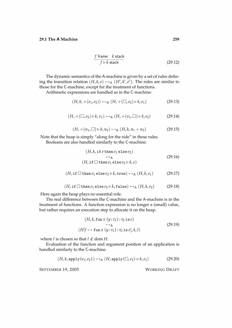
29.1 The A Machine 259
f frame k stack
f . k stack (29.12)
The dynamic semantics of the A-machine is given by a set of rules defin-ing the transition relation (H, k, e) 7→A (H′, k′, e′). The rules are similar tothose for the C-machine, except for the treatment of functions.
Arithmetic expressions are handled as in the C-machine:
(H, k, +(e1, e2)) 7→A (H, +(, e2) . k, e1) (29.13)
(H, +(, e2) . k, v1) 7→A (H, +(v1,) . k, e2) (29.14)
(H, +(n1,) . k, n2) 7→A (H, k, n1 + n2) (29.15)
Note that the heap is simply “along for the ride” in these rules.Booleans are also handled similarly to the C-machine:
(H, k, if e then e1 else e2)7→A
(H, if then e1 else e2 . k, e)(29.16)
(H, if then e1 else e2 . k, true) 7→A (H, k, e1) (29.17)
(H, if then e1 else e2 . k, false) 7→A (H, k, e2) (29.18)
Here again the heap plays no essential role.The real difference between the C-machine and the A-machine is in the
treatment of functions. A function expression is no longer a (small) value,but rather requires an execution step to allocate it on the heap.
(H, k, fun x (y:τ1):τ2 is e)7→A
(H[l 7→ fun x (y:τ1):τ2 is e], k, l)(29.19)
where l is chosen so that l /∈ dom H.Evaluation of the function and argument position of an application is
handled similarly to the C-machine.
(H, k, apply(e1, e2)) 7→A (H, apply(, e2) . k, e1) (29.20)
SEPTEMBER 19, 2005 WORKING DRAFT

260 29.1 The A Machine
(H, apply(, e2) . k, v1) 7→A (H, apply(v1,) . k, e2) (29.21)
Execution of a function call differs from the corresponding C-machineinstruction in that the function must be retrieved from the heap in orderto determine the appropriate instance of its body. Notice that the locationof the function, and not the function itself, is substituted for the functionvariable!
v1 loc H(v1) = fun f (x:τ1):τ2 is e(H, apply(v1,) . k, v2) 7→A (H, k, v1, v2/ f , xe) (29.22)
The A-machine preserves self-containment of the heap. This followsfrom observing that whenever a location is allocated, it is immediatelygiven a binding in the heap, and that the bindings of heap locations aresimply those functions that are encountered during evaluation.
Lemma 29.1If H is self-contained and (H, k, e) 7→A (H′, k′, e′), then H′ is also self-contained. Moreover, if FL(k) ∪ FL(e) ⊆ dom H, then FL(k′) ∪ FL(e′) ⊆dom H′.
It is not too difficult to see that the A-machine and the C-machine havethe same “observable behavior” in the sense that both machines deter-mine the same value for closed expressions of integer type. However, it issomewhat technically involved to develop a precise correspondence. Themain idea is to define the heap expansion of an A-machine state to be theC-machine state obtained by replacing all locations in the stack and expres-sion by their values in the heap. (It is important to take care that the loca-tions occurring in a value stored are themselves replaced by their values inthe heap!) We then prove that an A-machine state reaches a final state in ac-cordance with the transition rules of the A-machines iff its expansion doesin accordance with the rules of the C-machine. Finally, we observe that thevalue of a final state of integer type is the same for both machines.
Formally, let H(e) stand for the substitution
H(l1), . . . , H(ln)/l1, . . . , lne,
where dom H = l1, . . . , ln . Similarly, let H(k) denote the result of per-forming this substitution on every expression occurring in the stack k.
WORKING DRAFT SEPTEMBER 19, 2005
29.2 Garbage Collection 261
Theorem 29.2If (H, k, e) 7→A (H′, k′, e′), then (H(k), H(e)) 7→0,1
C (H′(k′), H′(e′)).
Notice that the allocation of a function in the A-machine corresponds tozero steps of execution on the C-machine, because in the latter case func-tions are values.
29.2 Garbage Collection
The purpose of the A-machine is to model the memory allocation that wouldbe required in an implementation of MinML. This raises the question ofgarbage, storage that is no longer necessary for a computation to complete.The purpose of a garbage collector is to reclaim such storage for further use.Of course, in a purely abstract model there is no reason to perform garbagecollection, but in practice we must contend with the limitations of finite,physical computers. For this reason we give a formal treatment of garbagecollection for the A-machine.
The crucial issue for any garbage collector is to determine which lo-cations are unnecessary for computation to complete. These are deemedgarbage, and are reclaimed so as to conserve memory. But when is a loca-tion unnecessary for a computation to complete? Consider the A-machinestate (H, k, e). A location l ∈ dom(H) is unnecessary, or irrelevant, for thismachine state iff execution can be completed without referring to the con-tents of l. That is, l ∈ dom H is unnecessary iff (H, k, e) 7→∗A (H′, •, v) iff(Hl , k, e) 7→∗A (H′′, •, v), where Hl is H with the binding for l removed, andH′′ is some heap.
Unfortunately, a machine cannot decide whether a location is unneces-sary!
Theorem 29.3It is mechanically undecidable whether or not a location l is unnecessaryfor a given state of the A-machine.
Intuitively, we cannot decide whether l is necessary without actually run-ning the program. It is not hard to formulate a reduction from the haltingproblem to prove this theorem: simply arrange that l is used to complete acomputation iff some given Turing machine diverges on blank input.
Given this fundamental limitation, practical garbage collectors mustemploy a conservative approximation to determine which locations are un-necessary in a given machine state. The most popular criterion is based
SEPTEMBER 19, 2005 WORKING DRAFT
262 29.2 Garbage Collection
on reachability. A location ln is unreachable, or inaccessible, iff there is nosequence of locations l1, . . . , ln such that l1 occurs in either the current ex-pression or on the control stack, and li occurs in li+1 for each 1 ≤ i < n.
Theorem 29.4If a location l is unreachable in a state (H, k, e), then it is also unnecessaryfor that state.
Each transition depends only on the locations occurring on the control stackor in the current expression. Some steps move values from the heap ontothe stack or current expression. Therefore in a multi-step sequence, execu-tion can depend only on reachable locations in the sense of the definitionabove.
The set of unreachable locations in a state may be determined by tracing.This is easily achieved by an iterative process that maintains a finite set ofof locations, called the roots, containing the locations that have been foundto be reachable up to that point in the trace. The root set is initialized tothe locations occurring in the expression and control stack. The tracingprocess completes when no more locations can be added. Having found thereachable locations for a given state, we then deem all other heap locationsto be unreachable, and hence unnecessary for computation to proceed. Forthis reason the reachable locations are said to be live, and the unreachableare said to be dead.
Essentially all garbage collectors used in practice work by tracing. Butsince reachability is only a conservative approximation of necessity, all prac-tical collectors are conservative! So-called conservative collectors are, in fact,incorrect collectors that may deem as garbage storage that is actually nec-essary for the computation to proceed. Calling such a collector “conserva-tive” is misleading (actually, wrong), but it is nevertheless common practicein the literature.
The job of a garbage collector is to dispose of the unreachable loca-tions in the heap, freeing up memory for later use. In an abstract settingwhere we allow for heaps of unbounded size, it is never necessary to col-lect garbage, but of course in practical situations we cannot afford to wasteunlimited amounts of storage. We will present an abstract model of a par-ticular form of garbage collection, called copying collection, that is widelyused in practice. The goal is to present the main ideas of copying collec-tion, and to prove that garbage collection is semantically “invisible” in thesense that it does not change the outcome of execution.
WORKING DRAFT SEPTEMBER 19, 2005
29.2 Garbage Collection 263
The main idea of copying collection is to simultaneously determinewhich locations are reachable, and to arrange that the contents of all reach-able locations are preserved. The rest are deemed garbage, and are re-claimed. In a copying collector this is achieved by partitioning storage intotwo parts, called semi-spaces. During normal execution allocation occurs inone of the two semi-spaces until it is completely filled, at which point thecollector is invoked. The collector proceeds by copying all reachable stor-age from the current, filled semi-space, called the from space, to the othersemi-space, called the to space. Once this is accomplished, execution con-tinues using the “to space” as the new heap, and the old “from space” isreclaimed in bulk. This exchange of roles is called a flip.
By copying all and only the reachable locations the collector ensuresthat unreachable locations are reclaimed, and that no reachable locationsare lost. Since reachability is a conservative criterion, the collector may pre-serve more storage than is strictly necessary, but, in view of the fundamen-tal undecidability of necessity, this is the price we pay for mechanical col-lection. Another important property of copying collectors is that their exe-cution time is proportion to the size of the live data; no work is expendedmanipulating reclaimable storage. This is the fundamental motivation forusing semi-spaces: once the reachable locations have been copied, the un-reachable ones are eliminated by the simple measure of “flipping” the rolesof the spaces. Since the amount of work performed is proportional to thelive data, we can amortize the cost of collection across the allocation of thelive storage, so that garbage collection is (asymptotically) “free”. However,this benefit comes at the cost of using only half of available memory at anytime, thereby doubling the overall storage required.
Copying garbage collection may be formalized as an abstract machinewith states of the form (H f , S, Ht), where H f is the “ from” space, Ht isthe “to” space, and S is the scan set, the set of reachable locations. Theinitial state of the collector is (H, S, ∅), where H is the “current” heap and∅ 6= S ⊆ dom(H f ) is the set of locations occurring in the program orcontrol stack. The final state of the collector is (H f , ∅, Ht), with an emptyscan set.
The collector is invoked by adding the following instruction to the A-machine:
(H, FL(k) ∪ FL(e), ∅) 7→∗G (H′′, ∅, H′)(H, k, e) 7→A (H′, k, e) (29.23)
The scan set is initialized to the set of free locations occurring in eitherthe current stack or the current expression. These are the locations that are
SEPTEMBER 19, 2005 WORKING DRAFT

264 29.2 Garbage Collection
immediately reachable in that state; the collector will determine those thatare transitively reachable, and preserve their bindings. Once the collectorhas finished, the “to” space is installed as the new heap.
Note that a garbage collection can be performed at any time! This cor-rectly models the unpredictability of collection in an implementation, butavoids specifying the exact criteria under which the collector is invoked. Asmentioned earlier, this is typically because the current heap is exhausted,but in an abstract setting we impose no fixed limit on heap sizes, preferringinstead to simply allow collection to be performed spontaneously accord-ing to unspecified criteria.
The collection machine is defined by the following two rules:
(H f [l = v], S ∪ l , Ht) 7→G (H f , S ∪ FL(v), Ht[l = v]) (29.24)
(H f , S ∪ l , Ht[l = v]) 7→G (H f , S, Ht[l = v]) (29.25)
The first rule copies a reachable binding in the “from” space to the “to”space, and extends the scan set to include those locations occurring in thecopied value. This ensures that we will correctly preserve those locationsthat occur in a reachable location. The second rule throws away any lo-cation in the scan set that has already been copied. This rule is necessarybecause when the scan set is updated by the free locations of a heap value,we may add locations that have already been copied, and we do not wantto copy them twice!
The collector is governed by a number of important invariants.
1. The scan set contains only “valid” locations: S ⊆ dom H f ∪ dom Ht;
2. The “from” and “to” space are disjoint: dom H f ∩ dom Ht = ∅;
3. Every location in “to” space is either in “to” space, or in the scan set:FL(Ht) ⊆ S ∪ dom Ht;
4. Every location in “from” space is either in “from” or “to” space: FL(H f ) ⊆dom H f ∪ dom Ht.
The first two invariants are minimal “sanity” conditions; the second twoare crucial to the operation of the collector. The third states that the “to”space contains only locations that are either already copied into “to” space,or will eventually be copied, because they are in the scan set, and hence in“from” space (by disjointness). The fourth states that locations in “from”
WORKING DRAFT SEPTEMBER 19, 2005
29.2 Garbage Collection 265
space contain only locations that either have already been copied or are yetto be copied.
These invariants are easily seen to hold of the initial state of the col-lector, since the “to” space is empty, and the “from” space is assumed tobe self-contained. Moreover, if these invariants hold of a final state, thenFL(Ht) ⊆ dom Ht, since S = ∅ in that case. Thus the heap remains self-contained after collection.
Theorem 29.5 (Preservation of Invariants)If the collector invariants hold of (H f , S, Ht) and (H f , S, Ht) 7→G (H′f , S′, H′t),then the same invariants hold of (H′f , S′, H′t).
The correctness of the collector follows from the following lemma.
Lemma 29.6If (H f , S, Ht) 7→G (H′f , S′, H′t), then H f ∪ Ht = H′f ∪ H′t and S ∪ dom Ht ⊆S′ ∪ dom H′t.
The first property states that the union of the semi-spaces never changes;bindings are only copied from one to the other. The second property statesthat the domain of the “to” space together with the scan set does not change.
From this lemma we obtain the following crucial facts about the collec-tor. Let S = FL(k) ∪ FL(e), and suppose that
(H, S, ∅) 7→∗G (H′′, ∅, H′).
Then we have the following properties:
1. The reachable locations are bound in H′: FL(k) ∪ FL(e) ⊆ dom H′.This follows from the lemma, since the inital “to” space and the finalscan set are empty.
2. The reachable data is correctly copied: H′ ⊆ H. This follows from thelemma, which yields H = H′′ ∪ H′.
SEPTEMBER 19, 2005 WORKING DRAFT

266 29.2 Garbage Collection
WORKING DRAFT SEPTEMBER 19, 2005

Bibliography
267