Progenesis QI for proteomics User Guide - Nonlinearstorage.nonlinear.com/webfiles/progenesis/qi-for-proteomics/v1.0/... · Progenesis QI for Proteomics User Guide 5 Restoring a Tutorial

Progenesis QI for proteomics User Guide

Analysis workflow guidelines for HDMse and MSe

data

Progenesis QI for Proteomics User Guide

Contents

Introduction ....................................................................................................................... 3

How to use this document ................................................................................................ 3

How can I analyse my own runs using LC-MS? ............................................................... 3

LC-MS Data used in this user guide ................................................................................. 3

Workflow approach to LC-MS run analysis ...................................................................... 4

Restoring a Tutorial Archive ............................................................................................. 5

Stage 1: Import Data and QC review of LC-MS data set ................................................. 6

Stage 2: Automatic Alignment of your data ...................................................................... 7

Stage 3: Licensing ............................................................................................................ 9

Stage 4: Review Alignment .............................................................................................. 9

Reviewing Quality of Alignment ...................................................................................... 11

Stage 5A: Filtering .......................................................................................................... 14

Stage 5B: Reviewing Normalisation ............................................................................... 18

Stage 6: Experiment Design Setup for Analysed Runs .................................................. 21

Stage 7: Validation, review and editing of results .......................................................... 24

Stage 8: Peptide Statistics on Selected Features .......................................................... 38

Stage 9: Identify peptides ............................................................................................... 42

Stage 10: Refine Identifications ...................................................................................... 45

Stage 11: Resolve Conflicts ........................................................................................... 47

Stage 12: Review Proteins ............................................................................................. 51

Stage 13: Protein Statistics ............................................................................................ 55

Stage 14: Exporting data ................................................................................................ 56

Stage 15: Reporting ........................................................................................................ 57

Appendix 1: Stage 1 Data Import and QC review of LC-MS data set ............................ 59

Appendix 2: Manual assistance of Alignment................................................................. 65

Appendix 3: Licensing runs (Stage 3) ............................................................................ 70

Appendix 4: Within-subject Design ................................................................................. 71

Appendix 5: Power Analysis (Peptide Stats) .................................................................. 73

Appendix 6: Waters Machine Specification .................................................................... 74


3

Introduction

This user guide takes you through a complete analysis of 9 LC-MS runs with 3 groups (3 replicate runs per group) using the unique Progenesis QI for Proteomics workflow. It starts with LC-MS data folders loading then Alignment, followed by Peak Detection that creates a list of interesting features (peptides) which are explored within Peptide Stats using multivariate statistical methods then onto Protein identity and Protein Stats.

To allow ease of use the tutorial is designed to start with the restoration of an Archived experiment where the data files have already been loaded. The document covers all the stages in the workflow, so if you are using your own data files please refer to Appendix 1 (page 59) then start at page 6.

How to use this document

You can print this user guide to help you work hands-on with the software. The complete user guide takes about 60 minutes. This means you can perform the first half focused on LC-MS run alignment and analysis then complete the second half of analysis exploring comparative differences and Protein identity at a convenient time.

How can I analyse my own runs using LC-MS?

You can freely explore the quality of your LC-MS data using Data Import and then licence your own LC-MS runs using this evaluation copy of Progenesis LC-MS. Instructions on how to do this are included in a section at the end of the user guide document.

LC-MS Data used in this user guide

For the purposes of this data set the MSE parameters were set to 250:125:1000 instead of the default settings as defined in Appendix 1 (page 59). This was to done to reduce the time taken to demo the data analysis.


4

Workflow approach to LC-MS run analysis

Progenesis QI for Proteomics adopts an intuitive Workflow approach to performing comparative LC-MS data analysis. The following user guide describes the various stages of this workflow (see below) focusing mainly on the stages from Alignment to Report.

Stage Description Page

LC-MS Import Data: Selection and review of data files for analysis 6 Automatic Alignment: Automatic Reference selection and Alignment 7

Licensing: allows licensing of individual data files when there 9 is no dongle attached (Appendix 3)

Review Alignment: review of automatic and manual run alignment 9

Filtering: defining filters for peaks based on Retention Time, 14 m/z , Charge and Number of Isotopes.

Review Normalisation: explaining LC-MS normalisation 18

Experiment Design Setup: defining one or more group set ups 21 for analysed aligned runs

Review Peak Picking: review and validate results, edit peak detection, 24 tag groups of peaks and select peaks for further analysis

Peptide Statistics: performing multivariate statistical analysis on 38 tagged and selected groups of peptides

Identify Peptides: managing export of MS/MS spectra to, and import 42 of peptide ids from Peptide Search engines

Refine Identifications: manage peptide ids and filters 45

Resolve Conflicts: validation and resolution of peptide id conflicts for 47 data entered from Database Search engines

Review proteins: review protein and peptide identity 51

Protein Statistics: multivariate statistical analysis on proteins 55

Report: generate a report for proteins and/or peptides 57


5

Restoring a Tutorial Archive

The data in the tutorial archive (Progenesis QI.P_Tutorial HDMSe.ProgenesisQIPArchive) is part of the Progenesis QI for Proteomics demo suite. Download and uncompress the zipped archive from the link on the website.

Now restore the uncompressed tutorial archive file. To do this, first locate the Tutorial Archive file from Progenesis QI for proteomics using the Open button and press Open.

This opens the 'Import from archive' dialog.

Select the Create a new experiment option and select the folder in which you placed the archive, using the icon (to the right).

Then press Import.

Note: use the Replace an existing experiment option if you want to over-write an existing version of the tutorial.

Tip: at each stage in the software there are links to more information and help on the website.


6

Stage 1: Import Data and QC review of LC-MS data set

The tutorial will now open at the Import Data stage (see below).

Each data file appears as a 2D representation of the run. At this stage you will be warned if any of the data files have been ‘centroided’ during the data acquisition and conversion process. Note: the Experiment Properties are available from the File menu. These were selected when the experiment was created (see Appendix 1, page 59). Tip: the 'Exclude areas from selected run' facility allows you to examine and exclude areas (usually early and/or late in the LC dimension (Retention Time)) that appear excessively noisy due to capture of data during column regeneration. This is not required for this data set. Note: use the Remove Run to remove run(s) from the current experiment. Now start the Alignment process


7

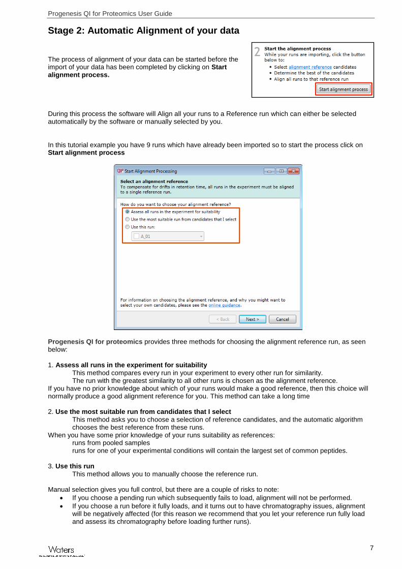
Stage 2: Automatic Alignment of your data

The process of alignment of your data can be started before the import of your data has been completed by clicking on Start alignment process. During this process the software will Align all your runs to a Reference run which can either be selected automatically by the software or manually selected by you. In this tutorial example you have 9 runs which have already been imported so to start the process click on Start alignment process

Progenesis QI for proteomics provides three methods for choosing the alignment reference run, as seen below: 1. Assess all runs in the experiment for suitability

This method compares every run in your experiment to every other run for similarity. The run with the greatest similarity to all other runs is chosen as the alignment reference.

If you have no prior knowledge about which of your runs would make a good reference, then this choice will normally produce a good alignment reference for you. This method can take a long time 2. Use the most suitable run from candidates that I select

This method asks you to choose a selection of reference candidates, and the automatic algorithm chooses the best reference from these runs.

When you have some prior knowledge of your runs suitability as references: runs from pooled samples runs for one of your experimental conditions will contain the largest set of common peptides.

3. Use this run

This method allows you to manually choose the reference run. Manual selection gives you full control, but there are a couple of risks to note:

If you choose a pending run which subsequently fails to load, alignment will not be performed.

If you choose a run before it fully loads, and it turns out to have chromatography issues, alignment will be negatively affected (for this reason we recommend that you let your reference run fully load and assess its chromatography before loading further runs).


8

For this tutorial we will select the first option (See Appendix 1, page 59 for more details on using the other options). You will now be asked if you want to align your runs automatically or manually.

Select automatically and click finish. The Alignment process starts with the automatic selection of A_01 as the reference

Once the Reference run has been chosen the automatic alignment is then performed. As the whole process proceeds you get information on what stage has been performed and also the % of the process that has been completed. When the Alignment completes you can either review the chromatography or go to the Review Alignment using the options on the Alignment Dialog. Click Review Alignment.


9

Stage 3: Licensing

This stage in the analysis workflow will only appear if you are using ‘Unlicensed’ data files to evaluate the software and have no dongle attached.

For details on how to use Licensing go to Appendix 3 (page 70) If you are using the tutorial archive, this page will not appear as the data files are licensed.

Stage 4: Review Alignment

At this stage Progenesis QI for proteomics Review Alignment opens displaying the alignment of the runs to the Reference run (A_01).

Vector Editing (Window A): is the main alignment area and displays the area defined by the current focus rectangle shown in Window C. The current run is displayed in green and the reference run is displayed in magenta. Here is where you can review in detail the vectors and also place the manual alignment vectors when required.

Transition (Window B): uses an alpha blend to animate between the current and reference runs. Before the runs are aligned, the features appear to move up and down. Once correctly aligned, they will appear to

Alignment Vector Alpha Blend

display animates between current

and reference runs

Current Focus

Current Run

(Green)

Reference Run

(Magenta)

A B

C D

Table of Alignment

Vectors and Scores


10

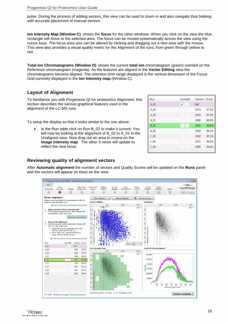
pulse. During the process of adding vectors, this view can be used to zoom in and also navigate thus helping with accurate placement of manual vectors.

Ion Intensity Map (Window C): shows the focus for the other windows. When you click on the view the blue rectangle will move to the selected area. The focus can be moved systematically across the view using the cursor keys. The focus area size can be altered by clicking and dragging out a new area with the mouse. This view also provides a visual quality metric for the Alignment of the runs, from green through yellow to red.

Total Ion Chromatograms (Window D): shows the current total ion chromatogram (green) overlaid on the Reference chromatogram (magenta). As the features are aligned in the Vector Editing view the chromatograms become aligned. The retention time range displayed is the vertical dimension of the Focus Grid currently displayed in the Ion Intensity map (Window C).

Layout of Alignment

To familiarize you with Progenesis QI for proteomics Alignment, this section describes the various graphical features used in the alignment of the LC-MS runs

To setup the display so that it looks similar to the one above:

In the Run table click on Run B_02 to make it current. You will now be looking at the alignment of B_02 to A_01 in the Unaligned view. Now drag out an area to review on the Image intensity map. The other 3 views will update to reflect the new focus.

Reviewing quality of alignment vectors

After Automatic alignment the number of vectors and Quality Scores will be updated on the Runs panel and the vectors will appear (in blue) on the view.


11

Where the alignment has worked well, the alignment views will look as below with the Ion Intensity Map showing green indicating good quality alignment and the Transition view showing features pulsing slightly but not moving up and down.

To simulate poor alignment, place a single manual vector on the Vector editing view (Window A). To do this click and drag out a single vector then release the mouse button. By doing this a single manual vector will appear with a length corresponding to the ‘drag’.

Note: the manual vector is red, to distinguish it from the automatic vectors (blue)

The effect of adding this incorrect manual vector is to reduce the Alignment score and also cause a significant proportion of the Alignment quality squares to turn red on the Ion Intensity Map (as shown below).

.

Using a Simulated miss-aligned example to explain the review process for alignment, the alignment looks as below with a region of poor alignment (highlighted in red).

Reviewing Quality of Alignment

At this point the quality metric, overlaid on the Ion Intensity Map as coloured squares, acts as a guide drawing your attention to areas of the alignment. These range from Good (Green) through OK (Yellow) to Needs review (Red). Drag out a ‘Focus’ area that corresponds to one of the coloured squares. Three example squares are examined here.


12

For a ‘green’ square the majority of the data appears overlapped (black) indicating good alignment. When viewed in the Transition view the data appears to pulse.

For a ‘yellow’ square some of the data appears overlapped (black) indicating OK alignment. When viewed in the Transition view some of the data appears to pulse.

For a ‘red’ square little if any of the data appears overlapped (black) indicating questionable alignment. When viewed in the Transition view little data appears to pulse.

Note: the coloured metric should be used as a guide. In cases where there are a few ‘isolated’ red squares this can also be indicative of ‘real’ differences between the two runs being aligned and should be considered when examining the overall score and surrounding squares in the current alignment.


13

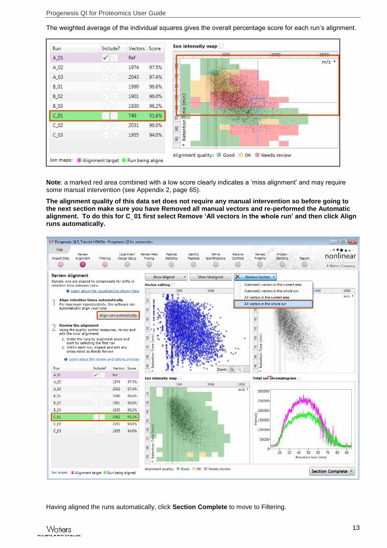
The weighted average of the individual squares gives the overall percentage score for each run’s alignment.

Note: a marked red area combined with a low score clearly indicates a ‘miss alignment’ and may require some manual intervention (see Appendix 2, page 65).

The alignment quality of this data set does not require any manual intervention so before going to the next section make sure you have Removed all manual vectors and re-performed the Automatic alignment. To do this for C_01 first select Remove ‘All vectors in the whole run’ and then click Align runs automatically.

Having aligned the runs automatically, click Section Complete to move to Filtering.


14

Stage 5A: Filtering

Now that you have reviewed your aligned Runs, you are ready to analyse them. Move to the Filtering stage, by either clicking on Section Complete (bottom right) or on Filtering on the workflow.

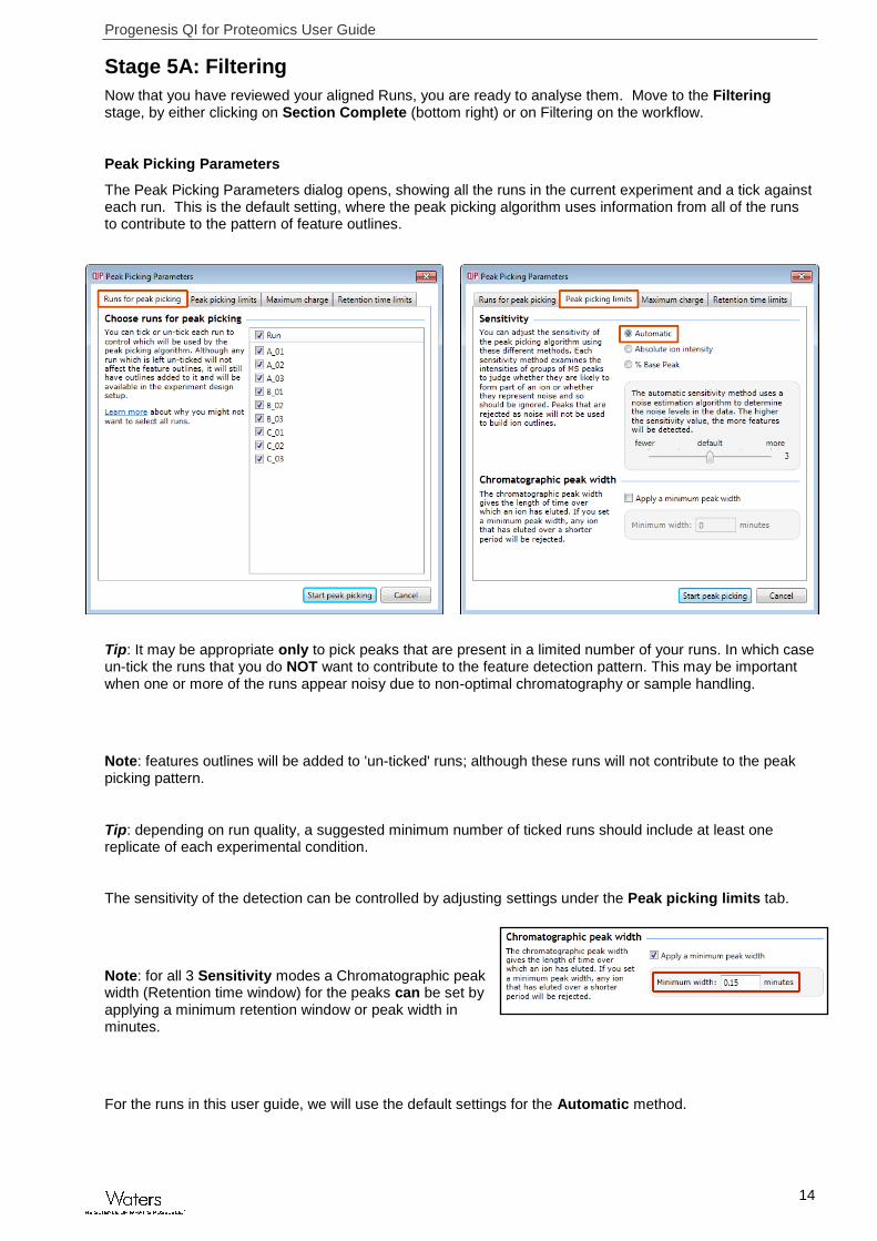
Peak Picking Parameters

The Peak Picking Parameters dialog opens, showing all the runs in the current experiment and a tick against each run. This is the default setting, where the peak picking algorithm uses information from all of the runs to contribute to the pattern of feature outlines.

Tip: It may be appropriate only to pick peaks that are present in a limited number of your runs. In which case un-tick the runs that you do NOT want to contribute to the feature detection pattern. This may be important when one or more of the runs appear noisy due to non-optimal chromatography or sample handling.

Note: features outlines will be added to 'un-ticked' runs; although these runs will not contribute to the peak picking pattern.

Tip: depending on run quality, a suggested minimum number of ticked runs should include at least one replicate of each experimental condition.

The sensitivity of the detection can be controlled by adjusting settings under the Peak picking limits tab.

Note: for all 3 Sensitivity modes a Chromatographic peak width (Retention time window) for the peaks can be set by applying a minimum retention window or peak width in minutes.

For the runs in this user guide, we will use the default settings for the Automatic method.


15

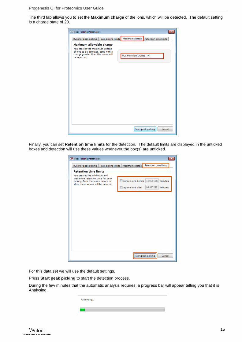
The third tab allows you to set the Maximum charge of the ions, which will be detected. The default setting is a charge state of 20.

Finally, you can set Retention time limits for the detection. The default limits are displayed in the unticked boxes and detection will use these values whenever the box(s) are unticked.

For this data set we will use the default settings.

Press Start peak picking to start the detection process.

During the few minutes that the automatic analysis requires, a progress bar will appear telling you that it is Analysing.


16

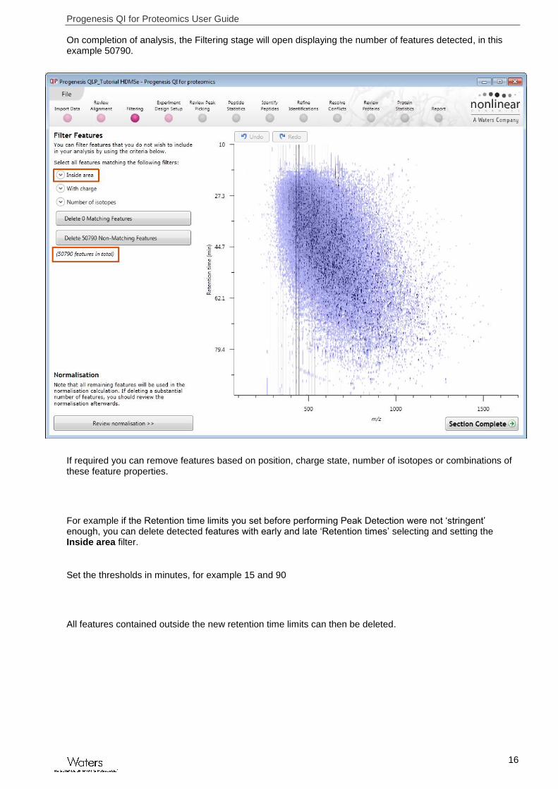
On completion of analysis, the Filtering stage will open displaying the number of features detected, in this example 50790.

If required you can remove features based on position, charge state, number of isotopes or combinations of these feature properties.

For example if the Retention time limits you set before performing Peak Detection were not ‘stringent’ enough, you can delete detected features with early and late ‘Retention times’ selecting and setting the Inside area filter.

Set the thresholds in minutes, for example 15 and 90

All features contained outside the new retention time limits can then be deleted.


17

To remove the features outside the retention time limits, as shown in blue, (in this case 56), press the Delete 56 Non-Matching Features button.

In addition to setting limits for ‘Retention time and m/z’, features can also be selected based on charge or the number of isotopes present. This allows you to refine the selection through a combination of feature properties.

For example, when With charge is selected the number of features present at each charge state is displayed, these can be selected accordingly.

Area limits, charge state and number of isotopes can be combined to refine the feature selection.

Tip: when filtering on one property of the feature i.e. charge state, make sure you have 'collapsed' the other filters (see right)


18

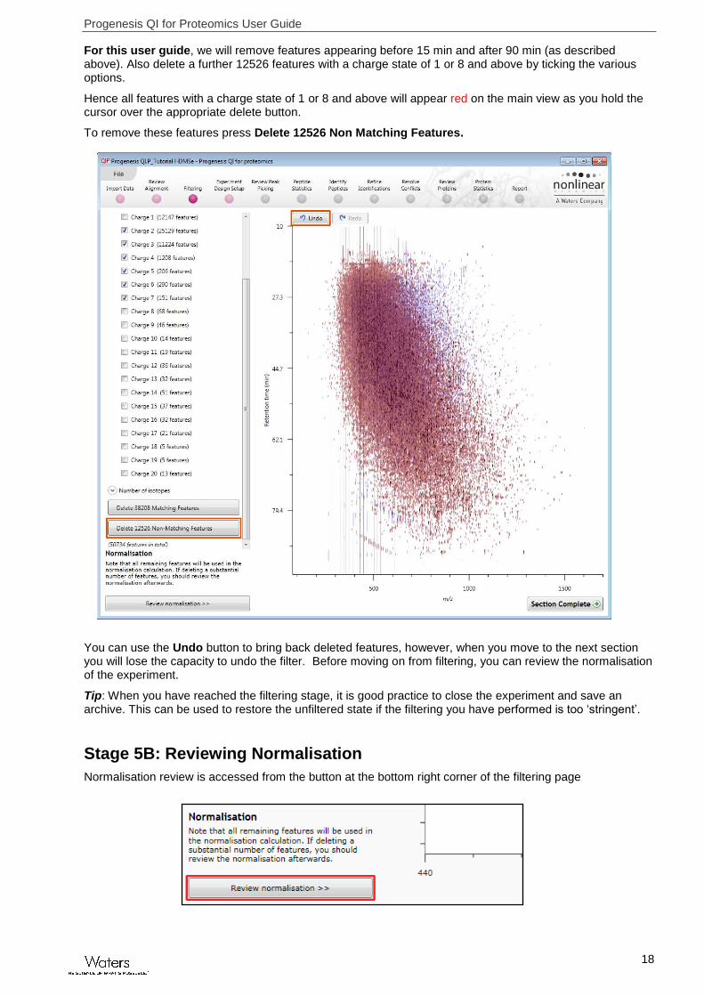
For this user guide, we will remove features appearing before 15 min and after 90 min (as described above). Also delete a further 12526 features with a charge state of 1 or 8 and above by ticking the various options.

Hence all features with a charge state of 1 or 8 and above will appear red on the main view as you hold the cursor over the appropriate delete button.

To remove these features press Delete 12526 Non Matching Features.

You can use the Undo button to bring back deleted features, however, when you move to the next section you will lose the capacity to undo the filter. Before moving on from filtering, you can review the normalisation of the experiment.

Tip: When you have reached the filtering stage, it is good practice to close the experiment and save an archive. This can be used to restore the unfiltered state if the filtering you have performed is too ‘stringent’.

Stage 5B: Reviewing Normalisation

Normalisation review is accessed from the button at the bottom right corner of the filtering page


19

If you have filtered out a number of features from the original detection pattern then the normalisation will update.

The Review Normalisation page will open displaying plots for the normalisation of all the features on each run.

This page in the workflow does not allow you to alter the Normalisation of your data but provides you with individual views for each run showing the data points used in the calculation of the normalisation factor for the run.

Alternatively, if you do not believe normalisation is necessary, you can opt to use un-normalised feature abundances for the rest of the analysis.

Normalisation factors are reported in the table to the left of the plots.

Calculation of Normalisation Factor:

Progenesis QI for proteomics will automatically select one of the runs that is 'least different' from all the other runs in the data and then set this to be the 'Normalising reference'. The run used, is shown above the table of Normalisation factors (in this example C_02).


20

For each sample run, each blue dot shows the log of the abundance ratio for a different feature (normalisation target abundance/run abundance).

The details for individual features can be viewed as you hold the cursor over the dots on the plot.

On the graph the features are shown ordered by ascending mean abundance. The normalisation factor is then calculated by finding the mean of the log abundance ratios of the features that fall within the ‘robust estimated limits’ (dotted red lines). Features outside these limits are considered to be outliers and therefore will not affect the normalisation.

Finally, if you do not wish to work with normalised data then you can use the raw abundances by switching off the normalisation.

Note: once you have identified the features, you can then apply the Normalise to a set of house keeping proteins by using this option to locate and select the features.

For this experiment, you should leave the Normalise to all proteins option selected.

Now return to filtering by clicking on the button on the bottom left of the screen

For this example, we DO NOT do any additional Filtering so click on Section complete.

Note: if you do any extra filtering then Normalisation recalculates as you move to the next stage in the Workflow.


21

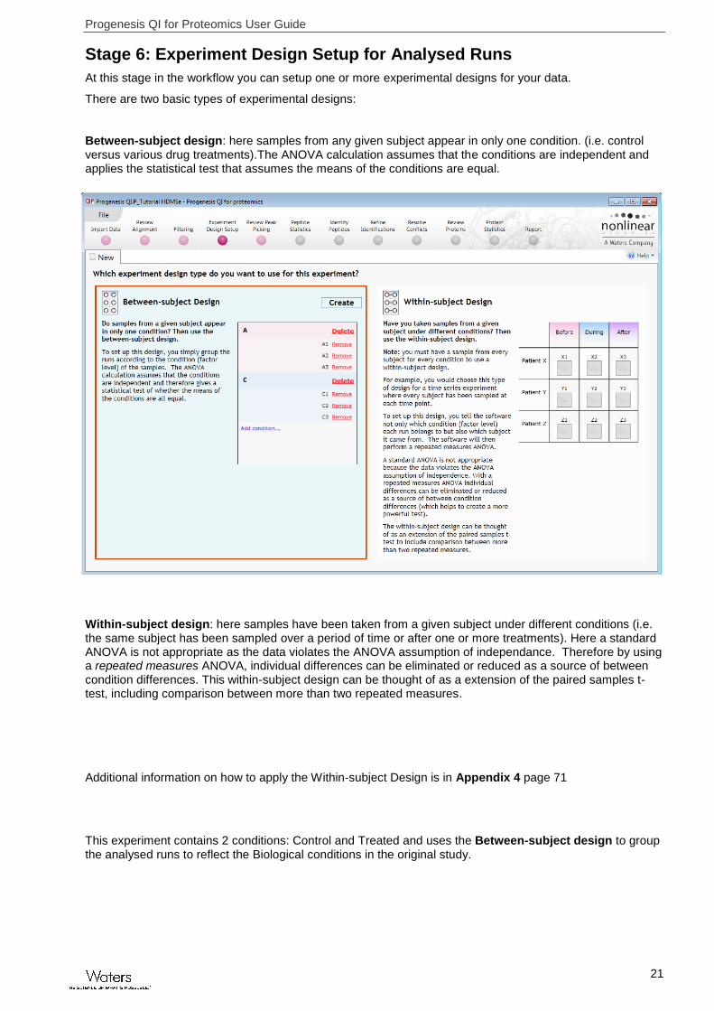
Stage 6: Experiment Design Setup for Analysed Runs

At this stage in the workflow you can setup one or more experimental designs for your data.

There are two basic types of experimental designs:

Between-subject design: here samples from any given subject appear in only one condition. (i.e. control versus various drug treatments).The ANOVA calculation assumes that the conditions are independent and applies the statistical test that assumes the means of the conditions are equal.

Within-subject design: here samples have been taken from a given subject under different conditions (i.e. the same subject has been sampled over a period of time or after one or more treatments). Here a standard ANOVA is not appropriate as the data violates the ANOVA assumption of independance. Therefore by using a repeated measures ANOVA, individual differences can be eliminated or reduced as a source of between condition differences. This within-subject design can be thought of as a extension of the paired samples t-test, including comparison between more than two repeated measures.

Additional information on how to apply the Within-subject Design is in Appendix 4 page 71

This experiment contains 2 conditions: Control and Treated and uses the Between-subject design to group the analysed runs to reflect the Biological conditions in the original study.


22

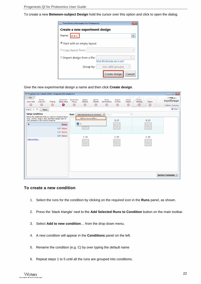
To create a new Between-subject Design hold the cursor over this option and click to open the dialog.

Give the new experimental design a name and then click Create design.

To create a new condition

1. Select the runs for the condition by clicking on the required icon in the Runs panel, as shown.

2. Press the ‘black triangle’ next to the Add Selected Runs to Condition button on the main toolbar.

3. Select Add to new condition… from the drop down menu.

4. A new condition will appear in the Conditions panel on the left.

5. Rename the condition (e.g. C) by over typing the default name

6. Repeat steps 1 to 5 until all the runs are grouped into conditions.


23

An alternative way to handling the grouping of this set and other larger (and more complex) experimental designs is to make use of sample tracking information that has been stored in a spread sheet at the time of sample collection and/or preparation. For this example there is a QIP_Conditions.spl file available in the Experiment Archive you restored at the beginning of this tutorial exercise. To use this approach select the Import design from file option from the New Experiment Design dialog. Then locate the QIP_Conditions file and select what to Group by, for example: Condition.

When Create design is pressed the new tab refreshes to allow you to adjust the conditions. Use Delete on the Conditions panel to remove conditions that are not required in this particular design.

Note: On deleting a condition the runs will reappear in the Runs window. Note: both designs are available as separate tabs. To move to the next stage in the workflow, Review Peak Picking, click Section Complete.


24

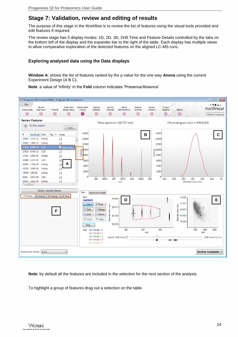
Stage 7: Validation, review and editing of results

The purpose of this stage in the Workflow is to review the list of features using the visual tools provided and edit features if required.

The review stage has 5 display modes: 1D, 2D, 3D, Drift Time and Feature Details controlled by the tabs on the bottom left of the display and the expander bar to the right of the table. Each display has multiple views to allow comparative exploration of the detected features on the aligned LC-MS runs.

Exploring analysed data using the Data displays

Window A: shows the list of features ranked by the p value for the one way Anova using the current Experiment Design (A B C).

Note: a value of ‘Infinity’ in the Fold column indicates ‘Presence/Absence’

Note: by default all the features are included in the selection for the next section of the analysis.

To highlight a group of features drag out a selection on the table.

E

B C

D

A

F


25

The 1D Display

Window B: displays the Mass spectrum for the current feature on the selected Run (in window D).

Window C: displays the Chromatogram for the current feature on the selected Run (in window D).

Window D: displays the details of the currently selected run. By default the selected run is an Aggregate view of all the aligned runs.

Details of individual runs can be viewed by using the ‘Run’ link and selecting the run you wish to view.

The feature editing tools are located in this window (see page 34 for functional explanation).

Clicking on the Expression Profile tab in Window D shows the comparative behaviour of the feature across the various biological groups based on group average normalised volume. The error bars show +/- 3 standard errors.

Window E: shows where the current feature is located on the LC-MS run by means of the ‘Green’ rectangle.

To change the current location, click on the image of the run (note: the retention time and m/z values update as you move the cursor around this view).

Note: doing this updates the focus of all the other windows.


26

You can also drag out an area (green square) on this view that will re-focus the other windows.

The 2D Display

Windows A, D and E: perform the same functions across all 4 display modes.

In the 2D Montage mode, Window B displays a montage of the current feature across all the aligned LC-MS runs.

The appearance of the Montage (window B) is controlled by the panel on the bottom left of the display.


27

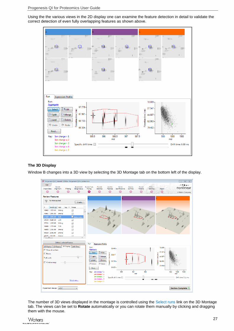
Using the the various views in the 2D display one can examine the feature detection in detail to validate the correct detection of even fully overlapping features as shown above.

The 3D Display

Window B changes into a 3D view by selecting the 3D Montage tab on the bottom left of the display.

The number of 3D views displayed in the montage is controlled using the Select runs link on the 3D Montage tab. The views can be set to Rotate automatically or you can rotate them manually by clicking and dragging them with the mouse.


28

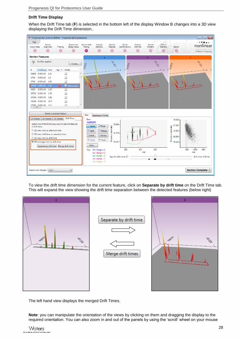
Drift Time Display

When the Drift Time tab (F) is selected in the bottom left of the display Window B changes into a 3D view displaying the Drift Time dimension..

To view the drift time dimension for the current feature, click on Separate by drift time on the Drift Time tab. This will expand the view showing the drift time separation between the detected features (below right)

The left hand view displays the merged Drift Times.

Note: you can manipulate the orientation of the views by clicking on them and dragging the display to the required orientation. You can also zoom in and out of the panels by using the ‘scroll’ wheel on your mouse


29

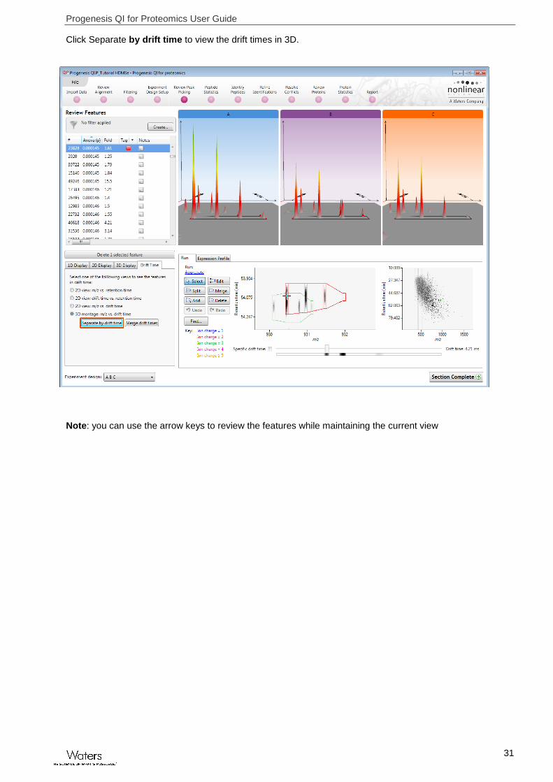
Note: you can step through the specific Drift Times (measured in milli seconds) for the current feature by clicking on the Specific drift time tick box at the bottom of the display.

The ‘crosshairs’ on the feature in the Run view identifies it as the current feature in the table.

As you move the slider over the intense areas, indicated below, all the views update to the corresponding drift time.


30

Note: the crosshairs will remain on the original feature in the table as you explore the Specific Drift times

When you un-tick the ‘Specific drift time, tick box the 3D views will return to showing the Merged Views for the current feature in the table.


31

Click Separate by drift time to view the drift times in 3D.

Note: you can use the arrow keys to review the features while maintaining the current view


32

Using Quick Tags to locate examples of Drift Time

In the previous section, describing how to view Drift Time, you will have noticed the presence of a red ‘Tag’ in the table next to the feature that we examined. Progenesis QI for proteomics allows you to assign tags based on the properties of detected features either through the manual sorting of the table or making use of the ‘Quick Tags’. These tags can be used to filter the list of displayed data in order to aid exploration of the data.

To create a Quick tag for all features demonstrating separation by Drift time, right click on the table. Select Quick Tags then Separated by drift time.

In the new tag dialog either accept or overtype the tag name.

When the tag is created it will appear against those features that meet the criteria for the creation of the tag, in this case:

It tags features that overlap in both m/z and retention time but do not show an overlap in the drift time dimension i.e. those features that drift time has separated

For example the features below is overlapping at the same m/z and RT but are separated in drift time

Now filter the table so that it currently only displays a list of features containing the separated by drift time tag.

Click on Create on the filter panel above the table.

This will open a Tag filter dialog, in this example, displaying that you have created assigned the Separated by drift time tag to 583 features in your experiment.


33

To display only those features containing this tag drag the Separated by drift time tag on to the Show panel and click OK.

When you apply the tag filter the table will now only display the features with the appropriate tag(s).

Note: with this Tag filter applied you can easily review the effect of Drift time separation for the features.

To remove the filter click on Edit, above the table, and Clear the filter followed by OK.


34

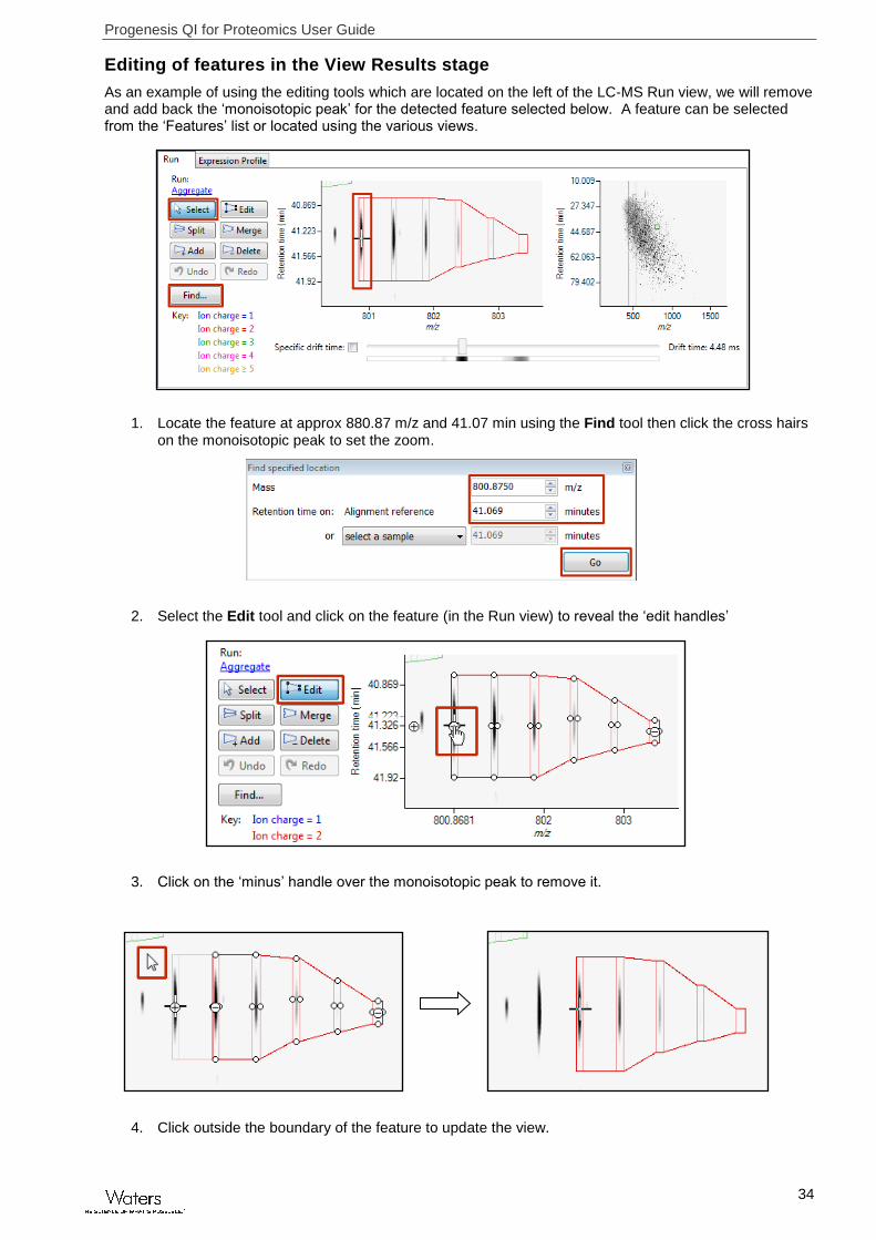
Editing of features in the View Results stage

As an example of using the editing tools which are located on the left of the LC-MS Run view, we will remove and add back the ‘monoisotopic peak’ for the detected feature selected below. A feature can be selected from the ‘Features’ list or located using the various views.

1. Locate the feature at approx 880.87 m/z and 41.07 min using the Find tool then click the cross hairs on the monoisotopic peak to set the zoom.

2. Select the Edit tool and click on the feature (in the Run view) to reveal the ‘edit handles’

3. Click on the ‘minus’ handle over the monoisotopic peak to remove it.

4. Click outside the boundary of the feature to update the view.


35

5. To add a peak to an existing feature, ensure that Edit is selected then click inside the feature to reveal the handles.

6. Click on the ‘plus’ handle on the peak to add it.

7. Then click outside the feature to update the view.

8. Note: If you are not satisfied with the editing use the Undo button and retry.

9. Finally note: that a tag is automatically added to the edited feature in the table and the features id. number is changed to the next available one at the end of the list.

The other tools: split, merge, add and delete behave in a similar fashion and their use can be combined to achieve the desired results.

Selecting and tagging features for Peptide Statistics

There are a number of ways to ‘refine’ your ‘Ranked List’ of analysed features before examining them with the Statistical tools in Peptide Statistics. These make use of simple ‘Selection’ and ‘Tagging’ tools that can be applied to the various groupings created in Stage 5 (page 21). An example is described below.

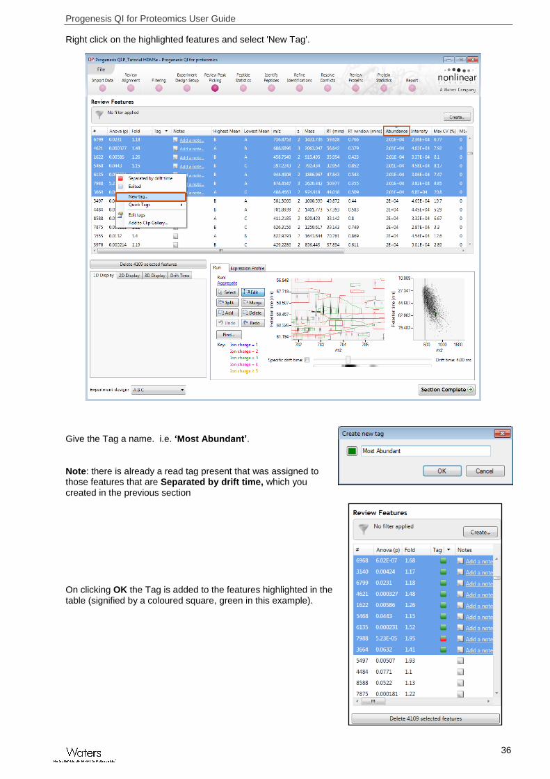
First expand the 'Features' table to show all the details by double clicking on the ‘Splitter Control’ to the right of the Review Features table.

Then order on Abundance and select all features with an Abundance > 2x104.


36

Right click on the highlighted features and select 'New Tag'.

Give the Tag a name. i.e. ‘Most Abundant’.

Note: there is already a read tag present that was assigned to those features that are Separated by drift time, which you created in the previous section

On clicking OK the Tag is added to the features highlighted in the table (signified by a coloured square, green in this example).


37

Now right click on any feature in the table and select Quick Tags this will offer you a number of standard tag options. Select Anova p-value.... Then set the threshold as required and adjust default name as required and click Create Tag.

Once this tag appears against features in the table right click on the table again and create another Quick Tag, this time for features with a Max fold change ≥ 2

The table now displays features with multiple tags.

The tags can be used to quickly focus the table on those features that display similar properties.

For example: to focus the table on displaying those features that are Most Abundant click on Create on the filter panel above the table.

Drag the tag on to the panel Show features that have all of these tags and press OK.

To move to the next stage in the workflow, Peptide Statistics, click Section Complete.


38

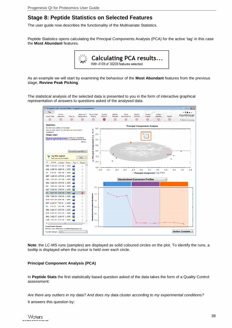
Stage 8: Peptide Statistics on Selected Features

The user guide now describes the functionality of the Multivariate Statistics.

Peptide Statistics opens calculating the Principal Components Analysis (PCA) for the active 'tag' in this case the Most Abundant features.

As an example we will start by examining the behaviour of the Most Abundant features from the previous stage, Review Peak Picking.

The statistical analysis of the selected data is presented to you in the form of interactive graphical representation of answers to questions asked of the analysed data.

Note: the LC-MS runs (samples) are displayed as solid coloured circles on the plot. To identify the runs, a tooltip is displayed when the cursor is held over each circle.

Principal Component Analysis (PCA)

In Peptide Stats the first statistically based question asked of the data takes the form of a Quality Control assessment:

Are there any outliers in my data? And does my data cluster according to my experimental conditions?

It answers this question by:


39

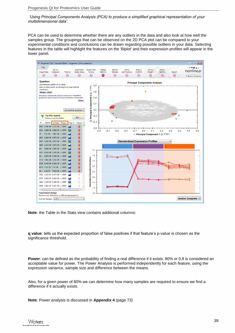
‘Using Principal Components Analysis (PCA) to produce a simplified graphical representation of your multidimensional data’.

PCA can be used to determine whether there are any outliers in the data and also look at how well the samples group. The groupings that can be observed on the 2D PCA plot can be compared to your experimental conditions and conclusions can be drawn regarding possible outliers in your data. Selecting features in the table will highlight the features on the 'Biplot' and their expression profiles will appear in the lower panel.

Note: the Table in the Stats view contains additional columns:

q value: tells us the expected proportion of false positives if that feature’s p-value is chosen as the significance threshold.

Power: can be defined as the probability of finding a real difference if it exists. 80% or 0.8 is considered an acceptable value for power. The Power Analysis is performed independently for each feature, using the expression variance, sample size and difference between the means.

Also, for a given power of 80% we can determine how many samples are required to ensure we find a difference if it actually exists.

Note: Power analysis is discussed in Appendix 4 (page 73)


40

Correlation Analysis

With the tag filter still set to display only the top 4109 Most Abundant features, we are going to explore the Correlation Analysis of these features.

To set up the Correlation Analysis using this filtered data set click on Ask another question (above the table)

A selection of 3 tools will appear in the form of questions.

Select the second option to explore ‘feature correlation based on similarity of expression profiles’

This time the statistically based question(s) being asked is:

‘Group my (selected) features according to how similar their expression profiles are’

The question is answered by:

‘Using Correlation analysis to evaluate the relationships between the (selected) features’ expression profiles’.


41

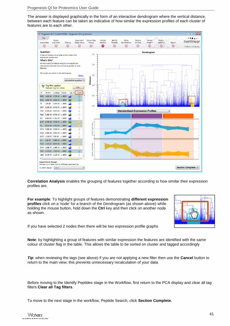
The answer is displayed graphically in the form of an interactive dendrogram where the vertical distance, between each feature can be taken as indicative of how similar the expression profiles of each cluster of features are to each other.

Correlation Analysis enables the grouping of features together according to how similar their expression profiles are.

For example: To highlight groups of features demonstrating different expression profiles click on a 'node' for a branch of the Dendrogram (as shown above) while holding the mouse button, hold down the Ctrl key and then click on another node as shown.

If you have selected 2 nodes then there will be two expression profile graphs

Note: by highlighting a group of features with similar expression the features are identified with the same colour of cluster flag in the table. This allows the table to be sorted on cluster and tagged accordingly

Tip: when reviewing the tags (see above) if you are not applying a new filter then use the Cancel button to return to the main view, this prevents unnecessary recalculation of your data.

Before moving to the Identify Peptides stage in the Workflow, first return to the PCA display and clear all tag filters Clear all Tag filters.

To move to the next stage in the workflow, Peptide Search, click Section Complete.


42

Stage 9: Identify peptides

Progenesis QI for proteomics is designed to perform peptide identifications either directly or by allowing you to export MS/MS peak lists in formats which can be used to perform peptide searches by various search engines. The resulting identifications can then be imported back into Progenesis QI for proteomics, using a number of different file types, and matched to your detected features.

For this example we are using the direct method MSE Search.

The Identify Peptides page currently displays the full list of the detected features in your experiment and some of their attributes, including the number of Identifications. If search results exist these can be cleared by clicking Clear all identifications.

Entering Search Parameters

Firstly you need to select the FASTA file containing peptide and protein identifications.

SWISSPROT-1 is provided with the installation of the software.

To add new Databanks in the form of FASTA files click on Edit… to open the Databank editor

Note: the SWISSPROT-1.0 is locked


43

For a new Databank you need to give it name, select the parsing rules and specify the location of the FASTA file, see the example below.

The new Data bank will appear in the left panel now click Save to return to the Search parameters.

If your databank is not already displayed then select it from the drop down list.

Expand the Common search parameters

The default settings are displayed:

Digest reagent: is set as Trypsin. Alternative Digest reagents are available from the list and additional ones can be added to the list using the Reagent editor...

Missed cleavages: is set as 1.

Maximum protein mass: is set at 250kDa

Modifications: are set Carbamidomethyl C (Fixed) and Oxidation M (variable). More modifications are available from the list and additional ones can be added to the list using the Modification editor…


44

Having selected the Databank and set the parameters, before Searching for identifications make sure that all of the runs are available for searching.

Depending on the search parameters the MSE Search can take some time

Once the Ion Accounting is complete, features with identifications are identified with a solid grey symbol and the number of identifications appears in the next column.

Details for the current features identifications are displayed in the table below and the Fragment ions for the current identification are displayed in the bottom panel.

Note: if you want to perform the search with a new set of parameters then first select Clear all identifications

In order to review, and refine the quality of the Peptide Search results click on the next stage in the workflow, Refine Identifications.


45

Stage 10: Refine Identifications

In this example we are going to apply a number of filters to ‘refine’ the quality of the Databank search.

As an example 'Acceptance Criteria' on which to base the sequential filtering of the Peptide results, the following thresholds will be applied:

Remove identifications with a Score less than 4

Remove identifications where less than 2 hits were returned

Remove all identifications where the Protein Description Contains the following: 'Putative', ‘Probable’, ‘Like’, ‘Potential’ and ‘Predicted’

To perform these filters, on the Batch detection options panel, set the Score to less than 4, then Delete matching search results.

Note: the search results matching the filter criteria turn pink and the total is displayed at the bottom of the table (1770 matching out of 28887)

Note: a dialog warns you of what you are about to delete

Now Clear all filters and then apply the next filter (Hits: less than 2)


46

Now in the Description first enter ‘Like’ and delete matching search results. Then enter the ‘regular expression’: regex:Puta|Prob|Pote|Pred and delete matching search results.

Having applied all the filters there will be 7981 search results remaining

To validate the Peptide search results at the protein level select the next stage in the workflow by clicking on Review Proteins.


47

Stage 11: Resolve Conflicts

This stage allows you to examine the behaviour of the identified peptides and choose to resolve any conflicts for the various peptide assignments at the protein level.

The number of conflicts you have to resolve will depend on the scope and stringency of the filters you apply at the Refine Identifications stage.

Note: the default Protein options for protein grouping and Protein quantitation are set as shown

This means that if you choose not to resolve the conflicts then a protein’s quantitation will be based on the non-conflicting or unique features (peptides).

If you choose not to resolve conflicts then click Section Complete to Review Proteins.

To proceed with resolving conflicts there are some simple rules that you can apply using this stage in the workflow

With Group similar proteins selected the additional members are indicated by a bracketed number located after the Accession number. As an example, when the cursor is held over the accession number the group members appear in a tool tip.

The bracketed number in the Peptides column indicates the number of unique peptides used for quantitation.


48

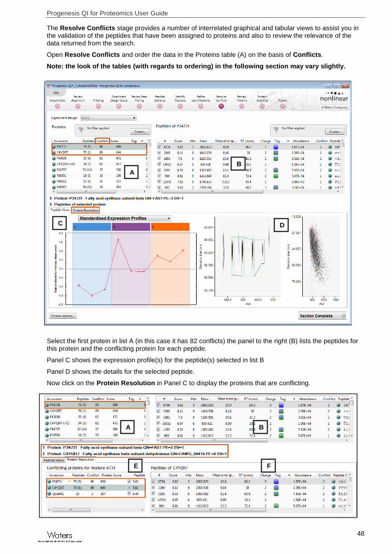
The Resolve Conflicts stage provides a number of interrelated graphical and tabular views to assist you in the validation of the peptides that have been assigned to proteins and also to review the relevance of the data returned from the search.

Open Resolve Conflicts and order the data in the Proteins table (A) on the basis of Conflicts.

Note: the look of the tables (with regards to ordering) in the following section may vary slightly.

Select the first protein in list A (in this case it has 82 conflicts) the panel to the right (B) lists the peptides for this protein and the conflicting protein for each peptide.

Panel C shows the expression profile(s) for the peptide(s) selected in list B

Panel D shows the details for the selected peptide.

Now click on the Protein Resolution in Panel C to display the proteins that are conflicting.

D

B

C

A

B A

F E


49

The lower left panel (E) displays the Conflicting proteins for the feature highlighted in panel (B) this includes the current protein in panel A as indicated by the orange ball to the right of the accession.

The Accession and description for the 2 proteins highlighted in Panels A and E are shown in the middle margin. As most of the features are conflicting between the 2 closely related proteins one simple way to resolve these conflicts is to favour the protein with the higher score and greater number of non-conflicting peptides.

One way to do this is to right click on the lower scoring protein in panel E which only has one unique peptide and turn off all its peptides

All the peptides are now switched off in panel B and all the entries for the lower scoring protein are set to zero. The higher scoring protein now has 66 non-conflicting peptides and only 3 conflicts

To resolve these remaining conflicts first order the conflicts in panel B and select the top one (which may still be selected) Panel B will display the peptides for this protein and the number of conflicts for each peptide. Panel E will also update to show the conflicting protein.

Again, favouring the protein with the higher score, but this time resolve the conflict by switching off (or un-assigning) the peptide in panel F for the protein with the lower score. By doing this the other 3 panels

B A

F E

B A

F E


50

update to show the change in conflicts.

Repeat this process until there are no conflicts remaining for the current protein in Panel A.

Now repeat using a similar approach for the next protein in Panel A, here the situation is similar.

Resolution of conflicts for this protein

Adopting a similar approach to the next protein favouring the protein with the highest score as each conflict is assessed.

In this case the first peptide for protein (P41797) has 5 conflicting proteins therefore move down the 5 conflicting proteins in panel E resolving the conflict in favour of this protein before moving on to the next peptide (which has 4 conflicts) in Panel B.

B A

F E


51

Using this approach, resolve this protein’s conflicts.

Note: where a protein has no or very few unique peptides and shares a large number of conflicts with a similarly named protein from a different species then right click and turn off all peptides

By adopting a combination of these rules you can work through the resolution of conflicts for the whole data set. Having completed Conflict resolution, move forward to Review Proteins.

Stage 12: Review Proteins

The Review Proteins stage opens displaying details for all proteins. You can now create tags at the level of the proteins. Right click on the table and create Quick Tags for proteins with an Anova p value ≤ 0.05 and Max Fold change ≥ 2.

Create the 2 Quick Tags


52

Corresponding protein tags are now displayed for the proteins.

To view the corresponding peptide measurements for the current protein either double click on the protein in the table or use the View peptide measurements below the table.


53

Note: by selecting all the peptides you can compare the pattern of expression across all the samples allowing you to identify ‘atypical’ behaviour of peptides assigned to the current protein.

Modified proteins can be located by specifically searching for proteins containing modified peptides. Use the Back button to return to the Proteins List and right click on it and select Modification from the list of Quick Tags.


54

To find those proteins containing peptides with Carbamidomethyl on cysteine residues enter Carbamidomethyl C. This will automatically provide a named tag when you click Create tag.

Repeat this for Oxidation of methionine residues.

To reduce the table to displaying only these proteins with modified peptides (oxidation on methionine) use the tag filter to focus on these proteins.

The proteins table will only display those proteins containing modified peptides.

Note: the Sequence Quick tag can be used to locate Proteins containing peptides with specific motifs.

Before leaving this stage in the workflow clear active Tag Filters.

Now move to the Protein Statistics section by clicking on Protein Statistics icon on the workflow at the top of the screen.


55

Stage 13: Protein Statistics

Protein Statistics opens with a Principal Components Analysis (PCA) for all the proteins displayed.

The Multivariate Stats can now be applied to all or subsets of proteins as determined by the current Tag filters. Allowing you to identify similar paterns of expression using the Correlation Analysis. Click on 2 of the branches (holding the Ctrl key down) to see diffeing patterns of expression.

Now move to the Report section to report on Proteins and /or peptides.


56

Stage 14: Exporting data

Protein measurement data can be exported from Progenesis QI for proteomics Workflow from the Review Peak Peaking stage onwards. Various data can be output and imported during the LC-MS workflow using

the File Menu options. The actual data available depends on the current stage of the Workflow.

As an example, try exporting data at the Review Proteins stage.

This opens a dialog that controls the content of the exported file. In this example we are only exporting a limited number of fields.

On saving the file the option to Open File is available.

The csv file opens displaying the exported Protein Measurements

Note: you can add addition columns to the csv file (shown above) containing numerical or descriptive information about the proteins. Then using the Import additional Protein Data… option on the File menu selectively import these extra columns into your experiment.


57

Stage 15: Reporting

The Report Design stage allows you to select what views you want to include in a report based on the list of currently selected proteins.

Note: this facility is used to generate Html reports on a limited selection of Proteins in your data. Creating a report on all the data in your experiment can take a long time

As an example we will create a report for only the proteins showing a Max Fold change of greater than 2.

1. First reduce the proteins to report on by selecting the ‘Max fold change ≥ 2’ tag. In this example it reduces the number of proteins in the table to 22.

2. Expand the various Report Design options (by default they are all selected)

3. Un-tick as shown below

4. Click Create Report

This opens a dialog to allow you to save the report, after which it will be opened in the form of a web page.


58

Click on the Accession No. in the proteins section of the Report and this will take you to the Assigned peptides for this protein

Having closed the report it can be reopened by double clicking on the saved html file.

Note: you can also copy and paste all or selected sections of the report to Excel and/or Word.

Note: there are separate panels for reporting on Proteins and Peptides.


59

Appendix 1: Stage 1 Data Import and QC review of LC-MS data set

You can use your own data files, either by directly loading the raw files (Waters, Thermo, Bruker, ABSciex and Agilent) or, for other Vendors, convert them to mzXML or mzML format first.

To create a new experiment with your files select New give your experiment a name. Then select data type, the default is ‘Profile data’.

Note: if you have converted or captured the data as centroided then select Centroided data and enter the Resolution for the MS machine used.

Click Create experiment to open the LC-MS Data Import stage of the workflow.

Select the ‘Import Data file format’, in this example they are Waters/SYNAPT data Then locate your data files using Import...


60

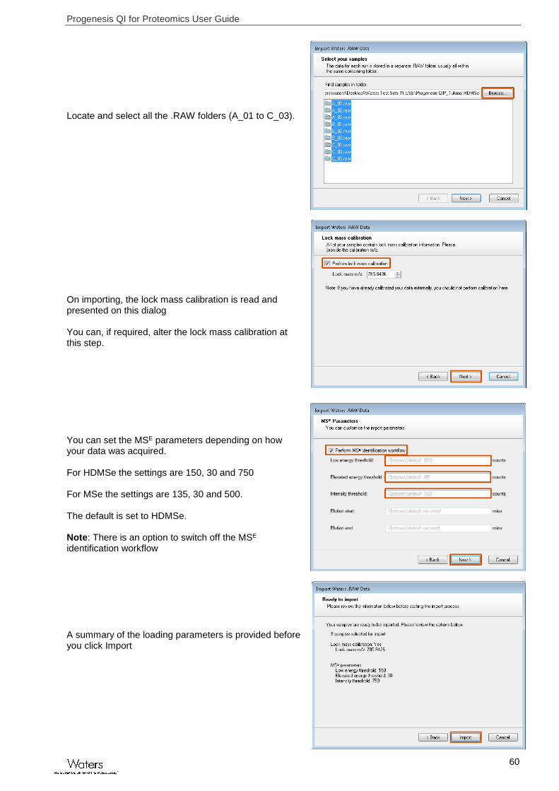
Locate and select all the .RAW folders (A_01 to C_03). On importing, the lock mass calibration is read and presented on this dialog You can, if required, alter the lock mass calibration at this step. You can set the MSE parameters depending on how your data was acquired. For HDMSe the settings are 150, 30 and 750 For MSe the settings are 135, 30 and 500. The default is set to HDMSe. Note: There is an option to switch off the MSE identification workflow A summary of the loading parameters is provided before you click Import


61

On loading the selected runs your data set will be automatically examined and the size of each file will be reduced by a ‘data modelling routine’, which reduces the data by several orders of magnitude but still retains all the relevant quantitation and positional information. Note: For a large number of files this may take some time. Each data file appears as a 2D representation of the run. At this stage you will be warned if any of the data files have been ‘centroided’ during the data acquisition and conversion process.

Note: as each data file is loaded the progress is reported in the Import Data list. The dialog below the run reports on the QC of the imported Data files. In this case ‘No problems found’ with the this data file Note: details of the current run appear on the top right of the view. Note: as the loading process starts you can also start the automatic alignment before the loading has completed. This is a 2 stage process that involves the selection of an Alignment Reference (either automatically or manually then the automatic alignment of all your runs to this Reference run. Click Start alignment process to start the automatic alignment of your runs.


62

Progenesis QI for proteomics provides three methods for choosing the alignment reference run, as seen below:

1. Assess all runs in the experiment for suitability

This method compares every run in your experiment to every other run for similarity. The run with the greatest similarity to all other runs is chosen as the alignment reference.

If you have no prior knowledge about which of your runs would make a good reference, then this choice will normally produce a good alignment reference for you. This method can take a long time 2. Use the most suitable run from candidates that I select

This method asks you to choose a selection of reference candidates, and the automatic algorithm chooses the best reference from these runs.

When you have some prior knowledge of your runs suitability as references:

runs from pooled samples runs for one of your experimental conditions will contain the largest set of common peptides.

3. Use this run

This method allows you to manually choose the reference run. Manual selection gives you full control, but there are a couple of risks to note:

If you choose a pending run which subsequently fails to load, alignment will not be performed.

If you choose a run before it fully loads, and it turns out to have chromatography issues, alignment will be negatively affected (for this reason we recommend that you let your reference run fully load and assess it’s chromatography before loading further runs).


63

Once you have selected how to handle the choice of Reference run you will now be asked if you want to Align your runs automatically or manually.

Select automatically and click finish. The Alignment process starts with the automatic selection of A_01 as the reference

Once the Reference run has been chosen the automatic alignment is performed. As the whole process proceeds you get information on what stage has been performed and also the % of the process that has been completed. Note: At this stage you have the option to Review the Chromatography or go straight to the review of the Automatic Alignment of your data.


64

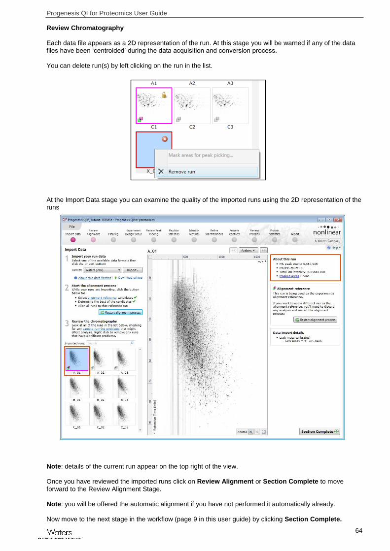
Review Chromatography Each data file appears as a 2D representation of the run. At this stage you will be warned if any of the data files have been ‘centroided’ during the data acquisition and conversion process. You can delete run(s) by left clicking on the run in the list.

At the Import Data stage you can examine the quality of the imported runs using the 2D representation of the runs

Note: details of the current run appear on the top right of the view. Once you have reviewed the imported runs click on Review Alignment or Section Complete to move forward to the Review Alignment Stage. Note: you will be offered the automatic alignment if you have not performed it automatically already. Now move to the next stage in the workflow (page 9 in this user guide) by clicking Section Complete.


65

Appendix 2: Manual assistance of Alignment

Approach to alignment

To place manual alignment vectors on a run (B_02 in this example):

1. Click on Run B_02 in the Runs panel, this will be highlighted in green and the reference run (A_01) will be highlighted in magenta.

2. You will need approximately 5 - 10 alignment vectors evenly distributed from top to bottom of the whole run.

3. First drag out an area on the Ion Intensity Map (C), this will reset the other 3 windows to display the same ‘zoomed’ area

Note: the features moving back and forwards between the 2 runs in the Transition window (B) indicating the misalignment of the two runs

Note: the Ion Intensity Map gives you a colour metric, visually scoring of the current alignment and an overall score is placed next to the Vectors column in the table. With each additional vector this score will update to reflect the overall quality of the alignment. The colour coding on the Ion intensity Map will also update with each additional vector

Note: The Total Ion Chromatograms window (D) also reflects the misalignment of the 2 runs for the current Retention Time range (vertical dimension of the current Focus grid in the Ion Intensity Map window).

A B

C D


66

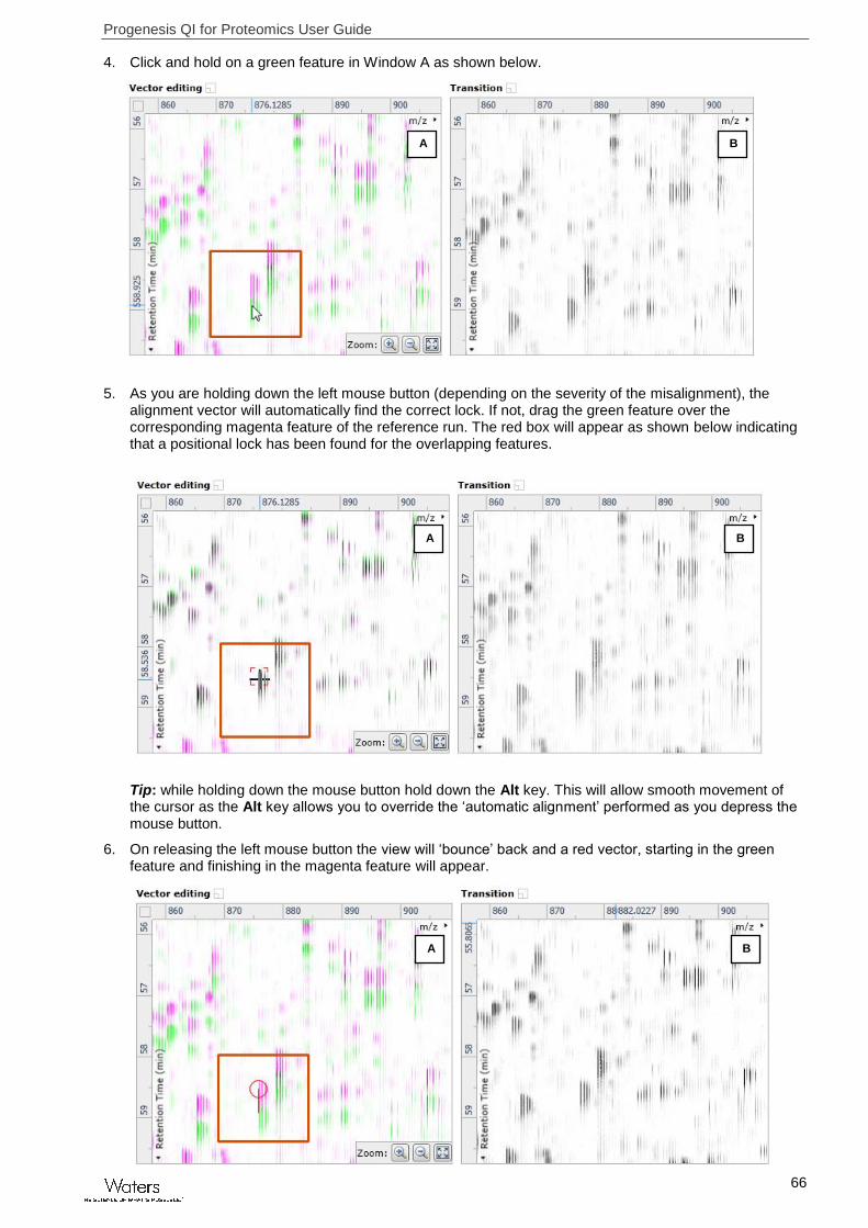
4. Click and hold on a green feature in Window A as shown below.

5. As you are holding down the left mouse button (depending on the severity of the misalignment), the alignment vector will automatically find the correct lock. If not, drag the green feature over the corresponding magenta feature of the reference run. The red box will appear as shown below indicating that a positional lock has been found for the overlapping features.

Tip: while holding down the mouse button hold down the Alt key. This will allow smooth movement of the cursor as the Alt key allows you to override the ‘automatic alignment’ performed as you depress the mouse button.

6. On releasing the left mouse button the view will ‘bounce’ back and a red vector, starting in the green feature and finishing in the magenta feature will appear.

A B

A B

A B


67

Note: an incorrectly placed vector is removed by right clicking on it in the Vector Editing window and selecting delete vector

7. Now click Show Aligned on the top tool bar to see the effect of adding a single vector.

8. With the placement of a single manual vector the increase in the proportion of the Ion Intensity Map (C) showing green is reflected in the improved alignment score in the table. Now click in the Ion Intensity Map to relocate the focus in order to place the next manual vector.

9. Adding an additional vector will improve the alignment further as shown below.

A B

C


68

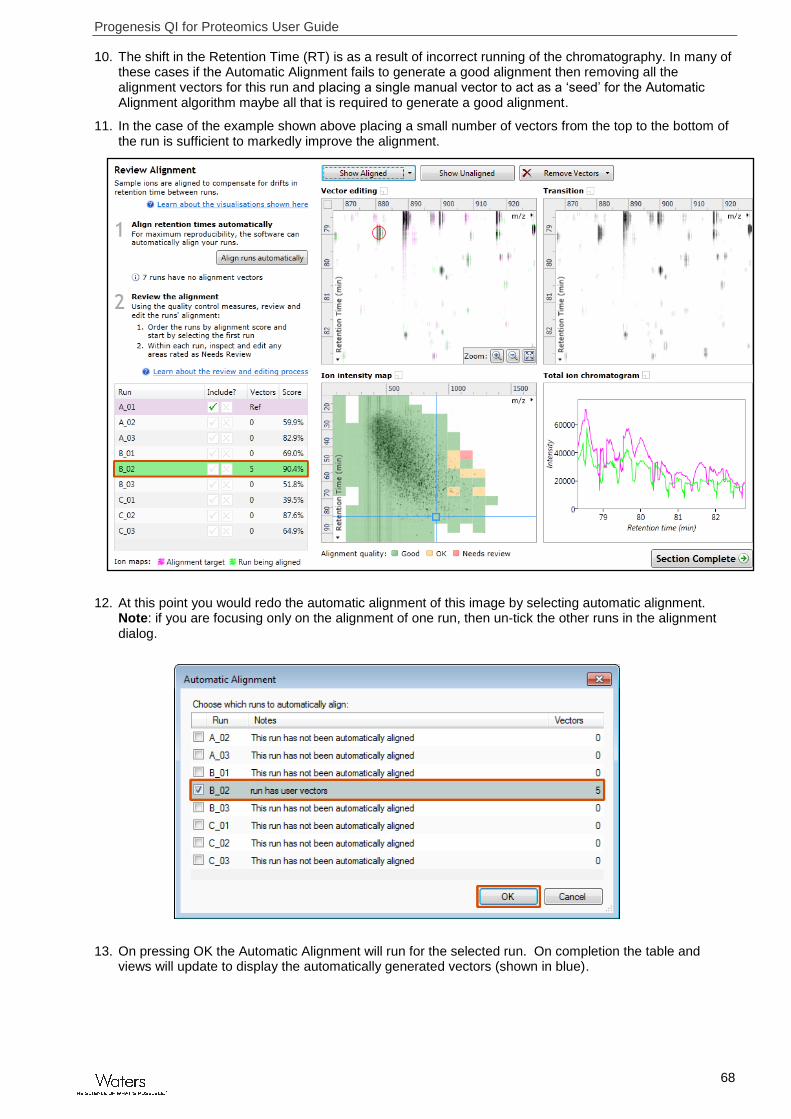
10. The shift in the Retention Time (RT) is as a result of incorrect running of the chromatography. In many of these cases if the Automatic Alignment fails to generate a good alignment then removing all the alignment vectors for this run and placing a single manual vector to act as a ‘seed’ for the Automatic Alignment algorithm maybe all that is required to generate a good alignment.

11. In the case of the example shown above placing a small number of vectors from the top to the bottom of the run is sufficient to markedly improve the alignment.

12. At this point you would redo the automatic alignment of this image by selecting automatic alignment. Note: if you are focusing only on the alignment of one run, then un-tick the other runs in the alignment dialog.

13. On pressing OK the Automatic Alignment will run for the selected run. On completion the table and views will update to display the automatically generated vectors (shown in blue).


69

14. Repeat this process for all the runs to be aligned.

The number of manual vectors that you add at this stage is dependent on the misalignment between the current run and the Reference run.

Note: In many cases only using the Automatic vector wizard will achieve the alignment.

Tip: a normal alignment strategy would be: to run the automatic alignment first for all runs, then order the alignments based on score. For low scoring alignments remove all the vectors and place 1 to 5 manual vectors to increase the score then perform automatic alignment. Then review the improved alignment score.

Also the ‘ease’ of addition of vectors is dependent on the actual differences between the LC-MS runs being aligned.

To review the vectors, automatic and manual, return to page 10

A B


70

Appendix 3: Licensing runs (Stage 3)

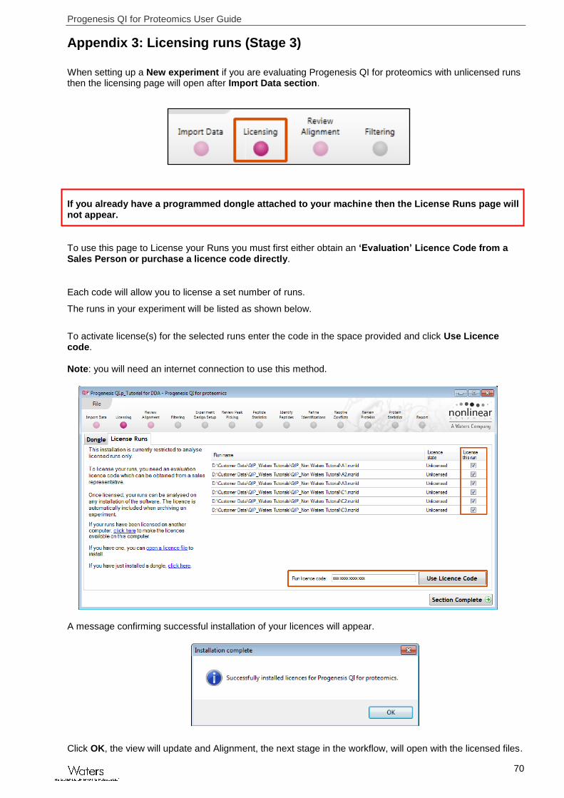
When setting up a New experiment if you are evaluating Progenesis QI for proteomics with unlicensed runs then the licensing page will open after Import Data section.

If you already have a programmed dongle attached to your machine then the License Runs page will not appear.

To use this page to License your Runs you must first either obtain an ‘Evaluation’ Licence Code from a Sales Person or purchase a licence code directly.

Each code will allow you to license a set number of runs.

The runs in your experiment will be listed as shown below.

To activate license(s) for the selected runs enter the code in the space provided and click Use Licence code. Note: you will need an internet connection to use this method.

A message confirming successful installation of your licences will appear.

Click OK, the view will update and Alignment, the next stage in the workflow, will open with the licensed files.


71

Appendix 4: Within-subject Design

To create a Within-subject Design for your data set select this option on the Experiment Design Setup page and enter the name of the design.

In this example there are 3 Subjects (i.e. patients A, B and C) who have been individually sampled: Before(1), During (2) and After (3) treatment

When the design page opens use the Add Subject and Add Condition buttons to create the matrix that fits your experimental design, over typing the names as required.


72

Then Drag and drop the Samples on to the correct 'cell' of the matrix.

You can create additional Experimental Designs using the New tab

All of these Experimental Designs are available at all the following stages in the Progenesis QI for proteomics workflow.


73

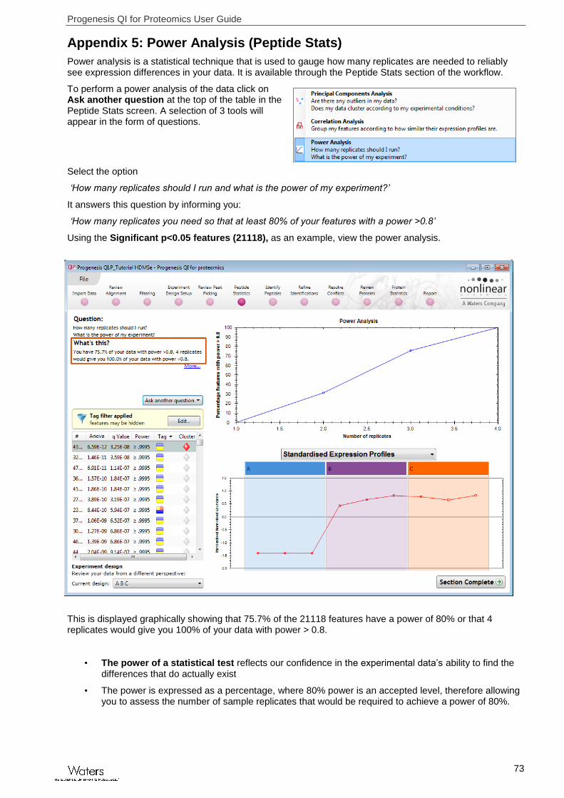
Appendix 5: Power Analysis (Peptide Stats)

Power analysis is a statistical technique that is used to gauge how many replicates are needed to reliably see expression differences in your data. It is available through the Peptide Stats section of the workflow.

To perform a power analysis of the data click on Ask another question at the top of the table in the Peptide Stats screen. A selection of 3 tools will appear in the form of questions.

Select the option

‘How many replicates should I run and what is the power of my experiment?’

It answers this question by informing you:

‘How many replicates you need so that at least 80% of your features with a power >0.8’

Using the Significant p<0.05 features (21118), as an example, view the power analysis.

This is displayed graphically showing that 75.7% of the 21118 features have a power of 80% or that 4 replicates would give you 100% of your data with power > 0.8.

• The power of a statistical test reflects our confidence in the experimental data’s ability to find the differences that do actually exist

• The power is expressed as a percentage, where 80% power is an accepted level, therefore allowing you to assess the number of sample replicates that would be required to achieve a power of 80%.


74

Appendix 6: Waters Machine Specification

This appendix provides information on the approximate time(s) taken at each stage and the total time taken to analyse a set of 9 (Phase 1) HDMSe runs on a Waters Demo Spec PC.

Machine Spec: Lenovo

Processor: Intel® Xeon® CPU 2.66GHz 12core X5650 @ 2.67GHz

RAM: 24.0 GB

System Type: 64-bit Operating System

File Folder Size: Each file folder (.RAW): 40.9 Gig

Analysis Stages: Per file Total

Import Data: Loading of Raw data per file 12min 2hr 6min Total for 9 files

Apex Background processing 1hr 05min(max) 9hr 45min Total for 9 files

(re-opening at Import Data) 20s

Alignment: Automatic alignment of data 8min 30s

(re-opening at Alignment) 10s

Peak Detection: Automatic Detection of data 14min 15s

(re-opening at Peak Detection) 10s

Identify Peptides: Performing MSE Search 14min 30s

(re-opening at Identify Peptides) 10s

Total Analysis Time Excluding Background Apex Processing 2hr 42min

Including Apex processing assuming pause for Apex 9hr 58min

Restoring Tutorial_A_Loading HDMSe.TOIP Experiment from archive 4min

Documents

Progenesis QI for proteomics User Guide - Nonlinearstorage.nonlinear.com/webfiles/progenesis/qi-for-proteomics/v1.0/... · Progenesis QI for Proteomics User Guide 5 Restoring a Tutorial