Embed Size (px)
Citation preview

CFD in Heat Transfer Equipment
Professor Bengt Sunden
Division of Heat Transfer
Department of Energy Sciences
Lund University
email: [email protected]

CFD ?
• CFD = Computational Fluid Dynamics;
Numerical solution methodology of
governing equations for mass
conservation, momentum and heat
transfer
• Focus on thermal issues; Computational
Heat Transfer or Numerical Heat
Transfer more appropriate names

Flow and Heat Transfer in Heat Transfer Equipment -
Governing Equations, steady state, Reynolds averaging
0jj
Ux
ji
ji
j
j
i
ji
ji
j
uuxx
U
x
U
xx
pUU
x
tu
x
T
xTU
xj
jjj
j
Pr

Turbulence Models
• Zero-equation models
• One-equation models
• Two-equation models
• Reynolds stress models
• Algebraic stress models
• Large Eddy Simulations (LES)
• Direct Numerical Simulations (DNS)

Turbulence models, RANS based
• Standard k-ε model
• RNG k-ε model
• Realizable k-ε model
• Standard k-ω model
• SST k-ω model
• Reynolds Stress Model
• v2f

Turbulence Models - Wall Effects
• Wall Functions Approach
• Low Reynolds Number Modelling

j
i
ji
jk
t
j
j
j x
Uuu
x
k
xkU
x)
Pr()(
kfC
x
Uuu
kC
xxU
x j
iji
j
t
j
j
j
2
2
1)Pr
()(
EXAMPLE OF A TWO-EQUATION
TURBULENCE MODEL
• Low-Re version k- model

EXAMPLE OF A TWO-EQUATION
TURBULENCE MODEL
• Low-Re version k- model, turbulent kinematic viscosity
/2kCft
μt= ρνt
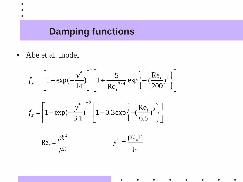
• Abe et al. model
2
4/3
2*
)200
Re(exp
Re
51)
14exp(1 t
t
yf
2
Rek
t yu n
*
2*
2Re1 exp( ) 1 0.3exp ( )
3.1 6.5
tyf
Damping functions

The general equation
• Arbitrary variable
Sxx
uxt jj
jj

NUMERICAL METHODS FOR PDEs -General
Purpose
• FDM - finite difference method
• FVM - finite volume method
• FEM - finite element method
• CVFEM - control volume finite element method
• BEM -boundary element

Control volume method-FVM
dS
B
n
Vthj
j j jV V V
UdV dV S dV
x x x
S S V
U dS dS S dV
Divergence theorem

Discretization - Sum over all the CV faces
IO
Ae
1 1
nf nf
f f ff f
C D S V
Sum up
S S V
U dS dS S dV

Computational grid and a control volume
• Two-dimensional case
S
N
EW P
n
e
s
w

Terms to be determined
• Convection flux Cf
• Diffusion flux Df
• Scalar value at a face Φf

CONVECTION-DIFFUSION TERMS
• CDS - central difference scheme
• UDS - upstream scheme
• HYBRID - hybrid scheme
• Power law scheme
• QUICK
• van Leer

PRESSURE - VELOCITY COUPLING
• SIMPLE (Semi-Implicit-Method-Pressure-
Linked-Equations)
• SIMPLEC (SIMPLE-Consistent)
• SIMPLEX (SIMPLE-extended)
• PISO (Pressure-Implicit-Splitting-
Operators)
• SIMPLER (SIMPLE-revised)

General algebraic equation, 2D case
aP P = aE E + aW W + aN N + aS S + b

Discretization - grid
Cartesian grid Body-fitted grid Unstructured grid

A typical multi-block BFC grid
0 2 4 6 8 10x/e
0
1
2
3
y/e

Why multi-block?
• To ease the grid-generation of complex
geometries
• Natural way for domain decomposition
used by parallel computation
• Better cache usage: smaller blocks are
easier to fit in the cache

Strategy for multi-blocking
• Keep most of the single-block code unchanged
• Same way of thinking as a single-block code
• Hide the multi-blocking from the end-user to ease the implementation of physical models
• Introduce no difference in the results

Grids - examples
-4 -3 -2 -1 0 1 2 3 4 5 6x/e0
1
2
3
y/e
0 2 4 6 8 10x/e
0
1
2
3
y/e
0 2 4 6 8 10x/e
0
1
2
3
y/e
Orthogonal-mb
Non-Orthogonal-mb
Non-Orthogonal-sb

Effect of multi-blocking
• On final results
• On convergence
• Execution speed

COMMERCIAL CFD COMPUTER CODES
• ANSYS FLUENT
• ANSYS CFX
• STAR CCM+
• COMSOL
• PHOENICS
• NUMECA
• CONVERGENT
• OPEN FOAM
• In-house codes

Examples of CFD in Heat Transfer
• Plate heat exchangers
• Radiators
• Impinging jet
• Impinging jet in cross flow

Ways to adopt CFD in heat exchanger analysis
and design
• 1) entire heat exchanger. a) detailed
simulations with large scales meshes,
b) local volume averaging or porous
media approach including distribution
of resistances
• 2) Modules or group of modules are
identified and streamwise periodic or
cyclic boundary conditions are
imposed

Gasketed plate-and-frame heat exchanger
Plate Heat Exchanger
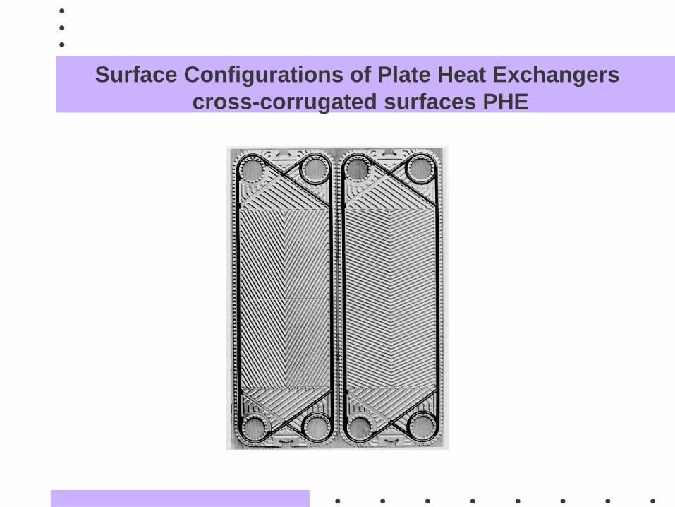
Surface Configurations of Plate Heat Exchangers
cross-corrugated surfaces PHE

Surface Configurations of Plate Heat Exchangers -
cross-corrugated surfaces PHE
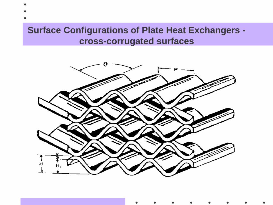
Surface Configurations of Plate Heat Exchangers -
cross-corrugated surfaces

Surface Configurations of Plate Heat Exchangers -
cross-corrugated surfaces – unit cell

Reynolds number
Definition:
w
m
2Re
w
m
2Re
w
m
2Re
w
m
2Re
w
m
2Re
Re = 2m/

Surface Configurations of Plate Heat Exchangers -
cross-corrugated surfaces

Plate Heat Exchangers : cross-corrugated surfaces,
hexahedron cells and boundary layer grid

Plate Heat Exchangers - cross-corrugated surfaces
• Re = 3000-5000
• Grid density ~ 89 500-985 000
computational cells

Plate Heat Exchangers - cross-corrugated surfaces;
Flow distribution

Plate Heat Exchangers - cross-corrugated surfaces; whole plate
calculations - flow field in neighborhood of contact points
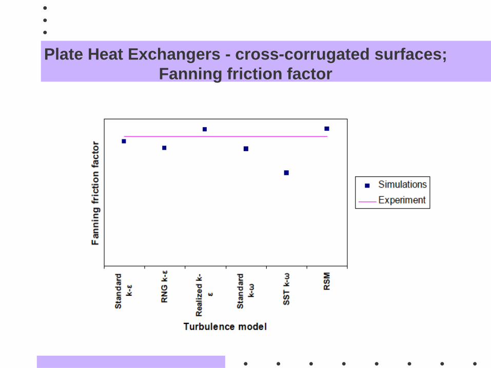
Plate Heat Exchangers - cross-corrugated surfaces;
Fanning friction factor

Plate Heat Exchangers - cross-corrugated surfaces;
Heat transfer coefficient

Surface Configurations of a Compact Heat Exchanger -
triangular duct with bumps for regenerators
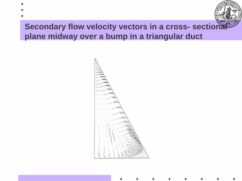
Secondary flow velocity vectors in a cross- sectional
plane midway over a bump in a triangular duct

Radiator in vehicles

Radiator – flat tubes and multilouvered fin geometry
HP
Hw

Radiator – porous media concept
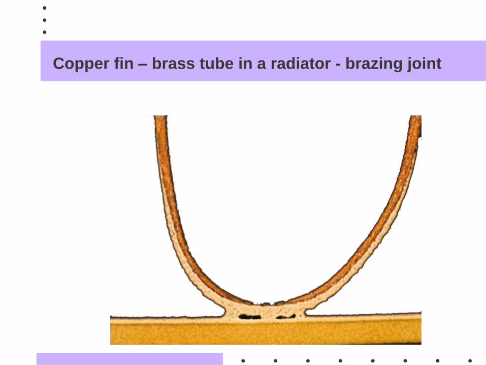
Copper fin – brass tube in a radiator - brazing joint

Copper fin – brass tube in a radiator - brazing joint

Brazing joints in radiators - example temperature
distribution

Multilouvered fin - sketch

Setup in Numerical Solution

Grid structure - inlet section

Grid structure - louver section

Grid structure - flow reverting section

Computed results - louvered fins
(a) Velocity at ReLp = 171 ( U = 2.5m/s )
(b) Temperature at ReLp = 171
(c) Velocity at ReLp = 513 ( U = 7.5 m/s )
(d) Temperature at ReLp = 513

Computed results – louvered fins
(a) Velocity at ReLp= 376 ( U=5.5 m/s )
(a) Temperature at ReLp= 376 ( U=5.5 m/s )
(c) Velocity vektors at ReLp=376

Computed results – louvered fins
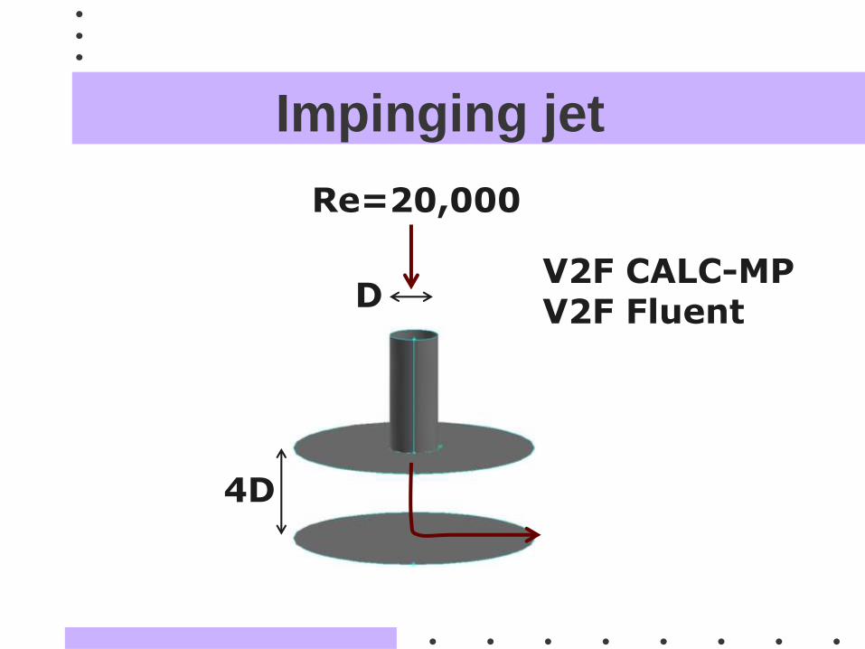
Impinging jet
Re=20,000
D
4D
V2F CALC-MPV2F Fluent

Mean velocities – comparisons with ANSYS
FLUENT
U
V
CALC-MP Fluent

Turbulence properties - Comparison with Fluent
TKE
ED
CALC-MP Fluent

Nusselt number on the impingement wall
0 1 2 3 4 50
50
100
150
200 Exp. Lee et al.
V2F Fluent
V2F CALC-MP
Nu
r/D

Jet Impinging on a Flat Surface
Re = 11000,
H/B = 4.0
0 2 4 6 8 10 12 14 16 18
0
10
20
30
40
50
60
70
80
90
100
Present simulation (EASM)
Present simulation (V2F Durbin 1995)
Exp. Gau & Lee (1992)
Exp. Schlunder (1977)
Exp. Gardon (1966)
Nu
x/B
The secondary peak of the Nusselt number is
predicted faithfully, using V2F.

Impinging jet in cross flow
Impingement cooling
Aircraft vertical take off and landing

Flow structure with cross flow
xX
Z
Y
Jet
Cro
ssFlo
w

Flow at the symmetry plane
M = 0.1 M = 0.2

Flow at two cross sections
-4 -2 0 2 4z/D
0
1
2
3
4
y/D
X = 1.5D
-4 -2 0 2 4z/D
0
1
2
3
4
y/D
Cross flow
Jet flow (Re = 20,000)
X = 20D

Horse shoe vortices
RANS LES
Cross flow
Jet flow (Re = 20,000)
Y/D = 3.2
Y/D = 2.3

Reynolds stresses
RANS
LES
uu uv

Nusselt number at symmetry line
5 6 7 8 9 10 11 12 13 14 150
50
100
150
200
250M = 0.1
LES
V2F
Nu
x/D

TOPICS NOT TREATED
• Implementation of boundary conditions
• Complex geometries
• Adaptive grid methods
• Local grid refinements
• Solution of algebraic equations
• Convergence and accuracy
• Parallel computing

Summary
CFD might be a useful tool in engineering R & D in
heat transfer
Arbitrary geometries can be handled decently but
may require a huge amount of grid points
Computer demanding for complete real
geometries
Turbulence modeling is critical or a weakness