Embed Size (px)
Citation preview
1
Prof. Ji Chen
Notes 22
Antennas and Radiation
ECE 3317
Spring 2014
x
y
z
Il
0 dB
30�30�
60�
120�
150� 150�
120�
60�
m
0
-10 dB
-20 dB
-30 dB
z
2
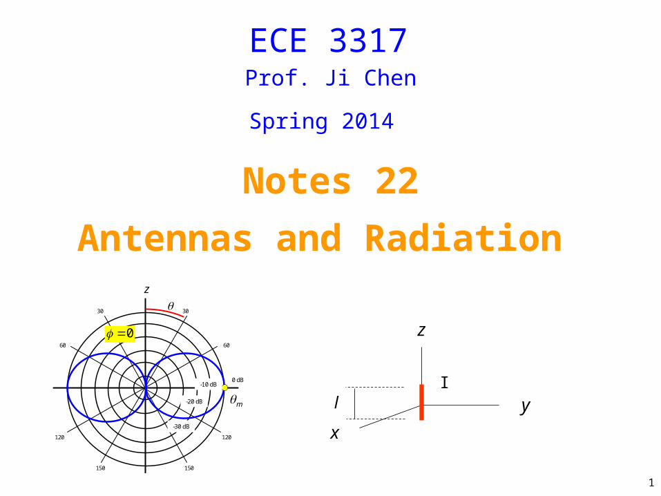
Antenna Radiation
We consider here the radiation from an arbitrary antenna.
The far-field radiation acts like a plane wave going in the radial direction.
+-
x
y
z
r
, ,r r
r "far field"
S
3
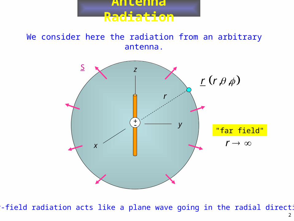
How far do we have to go to be in the far field?
This is justified from later analysis.
+-
r
, ,r r Sphere of minimum diameter D that encloses the antenna.
2
0
2Dr
Antenna Radiation (cont.)
4
Antenna Radiation (cont.)
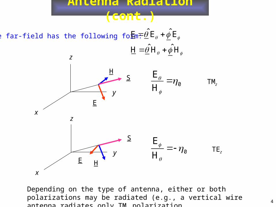
The far-field has the following form: ˆ ˆE E E
ˆ ˆH H H
0
E
H
0
E
H
x
y
z
E
HS
x
y
z
HE
S
TMz
TEz
Depending on the type of antenna, either or both polarizations may be radiated (e.g., a vertical wire antenna radiates only TMz polarization.
5
Antenna Radiation (cont.)
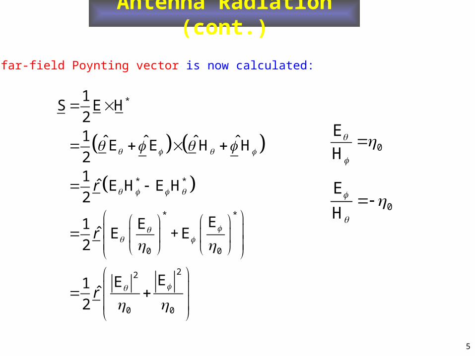
The far-field Poynting vector is now calculated:
*
* *
* *
0 0
22
0 0
1S E H
21 ˆ ˆ ˆ ˆE E H H21
ˆ E H E H2
EE1ˆ E + E
2
EE1ˆ
2
r
r
r
0
E
H
0
E
H
6
Antenna Radiation (cont.)
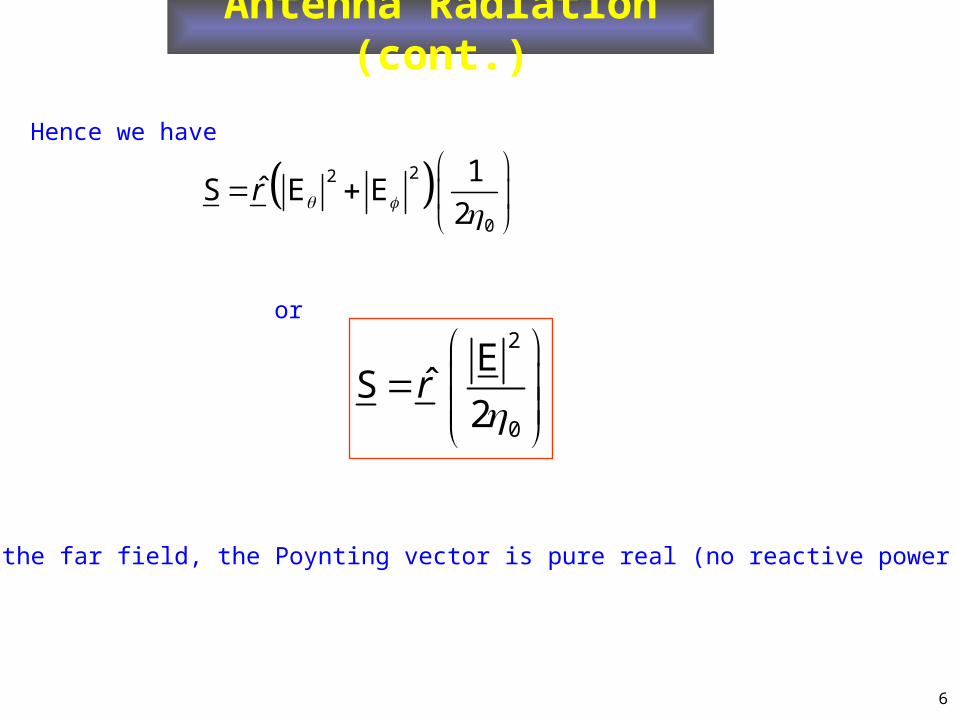
Hence we have
22
0
1ˆS E E
2r
2
0
EˆS
2r
or
Note: In the far field, the Poynting vector is pure real (no reactive power flow).
7
Radiation Pattern
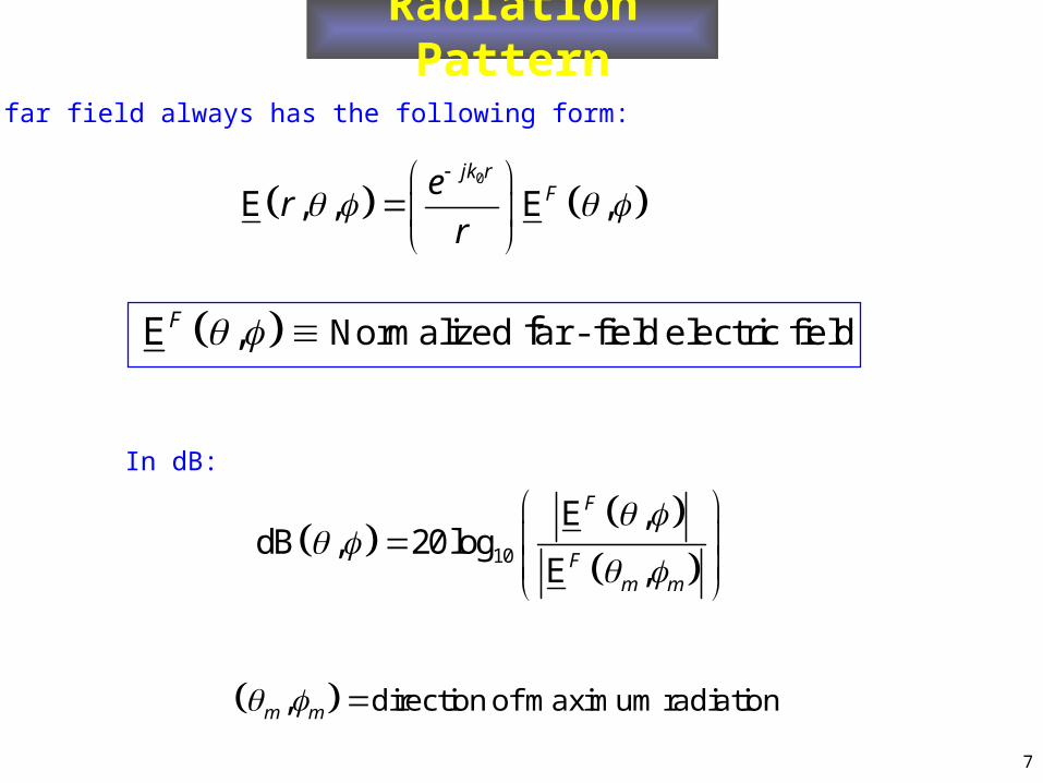
The far field always has the following form:
0
E , , E ,jk r
Fer
r
E ,F Normalized ar - field electric fieldf
In dB:
10
E ,dB , 20log
E ,
F
Fm m
,m m direction of maximum radiation
8
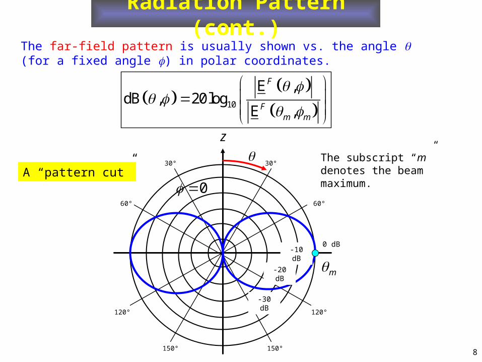
Radiation Pattern (cont.)The far-field pattern is usually shown vs. the angle (for a fixed angle ) in polar coordinates.
10
E ,dB , 20log
E ,
F
Fm m
The subscript “m” denotes the beam maximum.
0 dB
30°30°
60°
120°
150° 150°
120°
60°
m
0
-10 dB
-20 dB
-30 dB
z
A “pattern cut”
9
Radiated Power
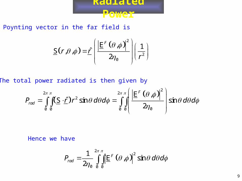
The Poynting vector in the far field is
2
20
E , 1ˆS , ,
2
F
r rr
The total power radiated is then given by
2
2 22
00 0 0 0
E ,ˆS sin sin
2
F
radP r r d d d d
Hence we have
2
2
0 0 0
1E , sin
2F
radP d d
10
Directivity
In dB,
2
S ,,
/ 4r
rad
D rP r
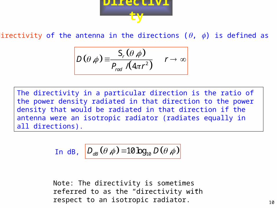
The directivity in a particular direction is the ratio of the power density radiated in that direction to the power density that would be radiated in that direction if the antenna were an isotropic radiator (radiates equally in all directions).
10, 10 log ,dBD D
The directivity of the antenna in the directions (, ) is defined as
Note: The directivity is sometimes referred to as the “directivity with respect to an isotropic radiator.”
11
Directivity (cont.)
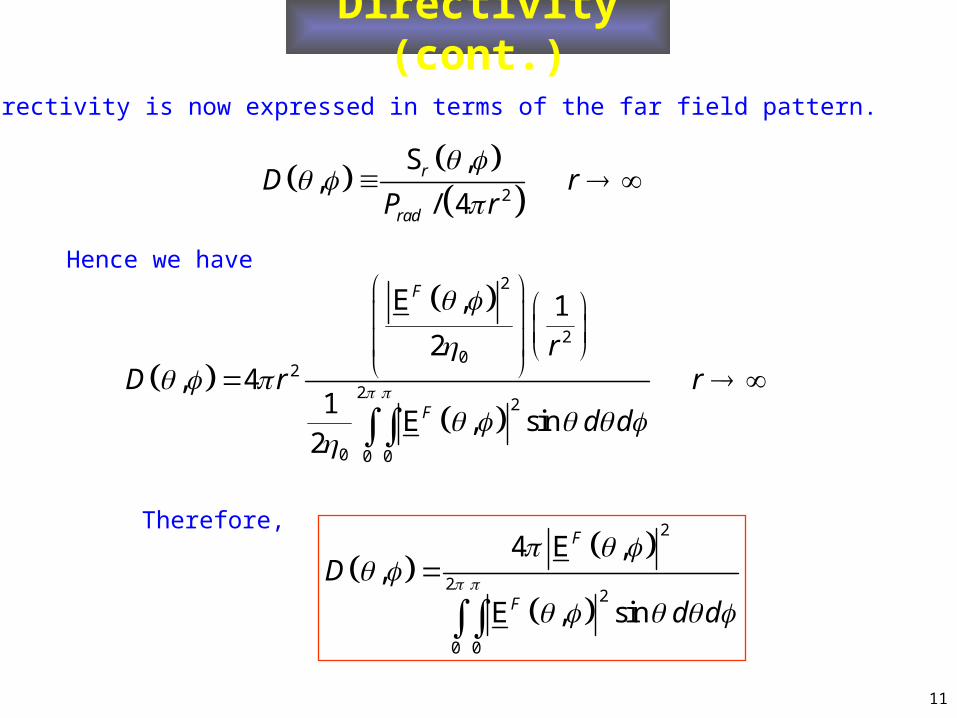
The directivity is now expressed in terms of the far field pattern.
2
S ,,
/ 4r
rad
D rP r
2
20
22
2
0 0 0
E , 1
2, 4
1E , sin
2
F
F
rD r r
d d
Therefore,
2
22
0 0
4 E ,,
E , sin
F
F
D
d d
Hence we have
12
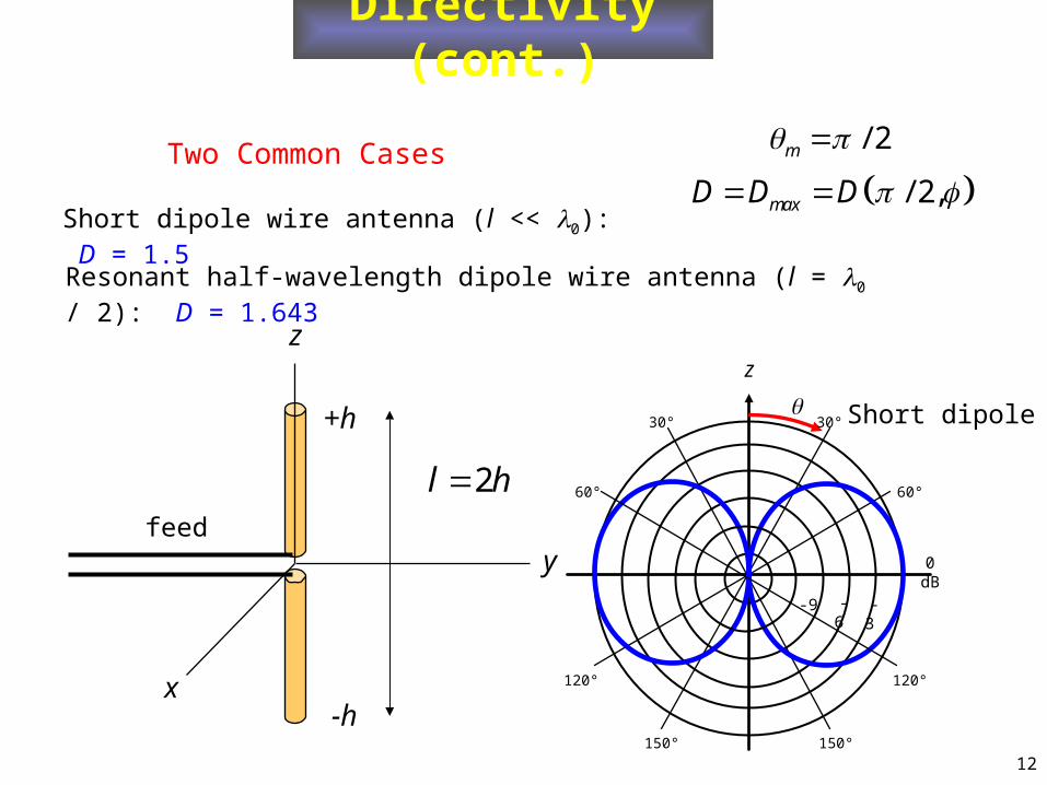
Directivity (cont.)
Two Common Cases
Short dipole wire antenna (l << 0): D = 1.5
Resonant half-wavelength dipole wire antenna (l = 0 / 2): D = 1.643
y
+h
z
x-h
feed
2l h
/ 2,maxD D D
/ 2m
-9 -3 -6
0 dB
30°30°
60°
120°
150° 150°
120°
60°
z
Short dipole
13
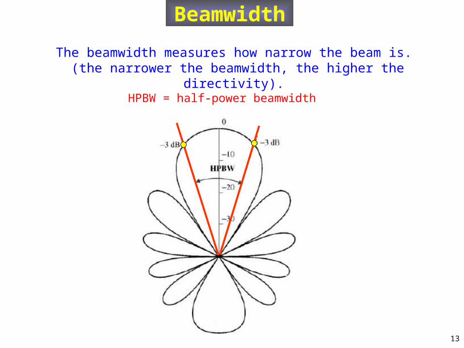
Beamwidth
The beamwidth measures how narrow the beam is. (the narrower the beamwidth, the higher the directivity).
HPBW = half-power beamwidth
14
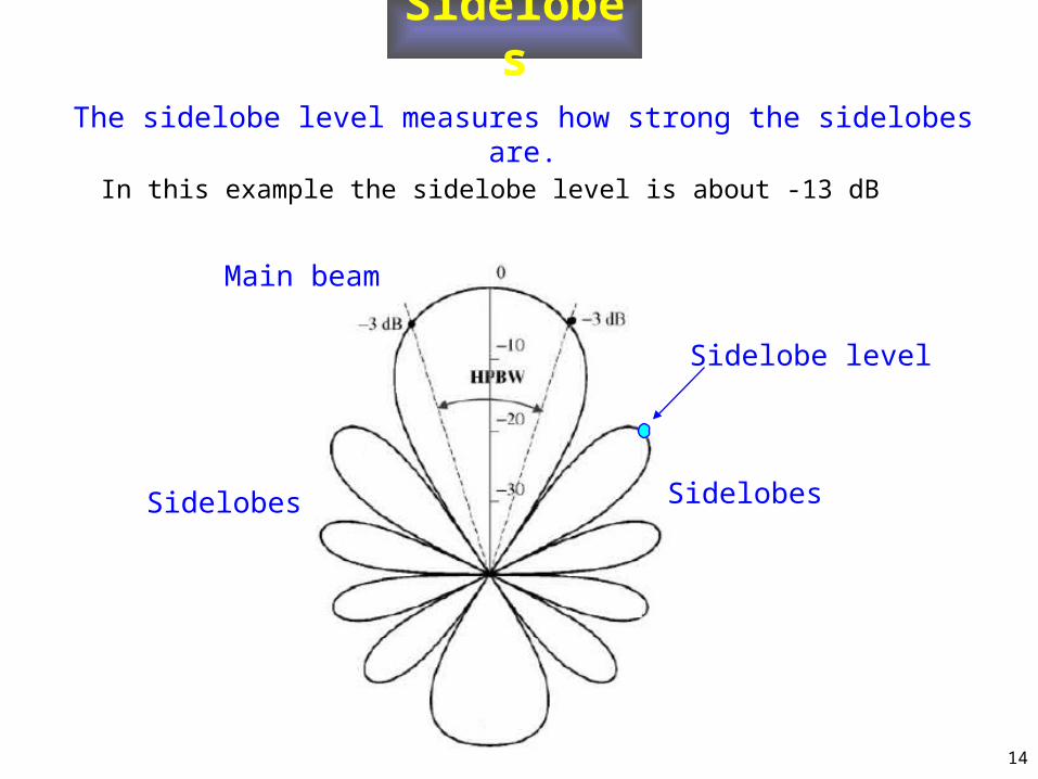
Sidelobes
The sidelobe level measures how strong the sidelobes are.
In this example the sidelobe level is about -13 dB
Sidelobes
Sidelobe level
Sidelobes
Main beam
15
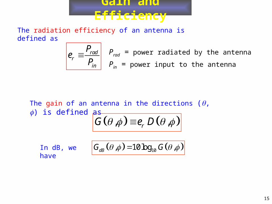
Gain and Efficiency
The radiation efficiency of an antenna is defined as
radr
in
Pe
P Prad = power radiated by the antenna
Pin = power input to the antenna
The gain of an antenna in the directions (, ) is defined as
, ,rG e D
10, 10 log ,dBG G In dB, we have
16
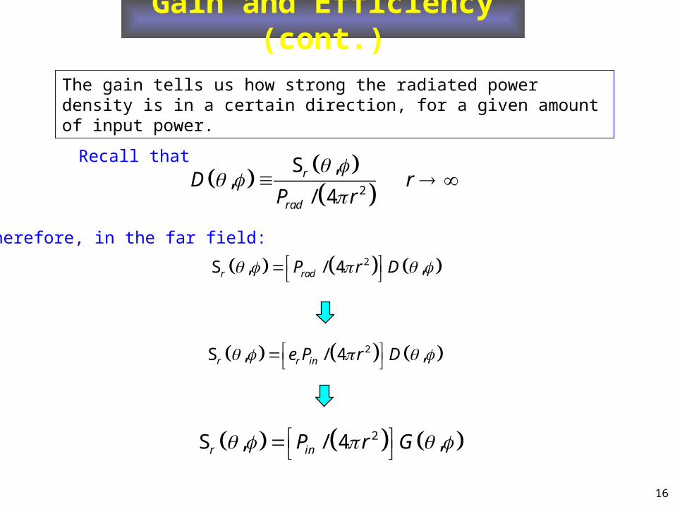
Gain and Efficiency (cont.)
The gain tells us how strong the radiated power density is in a certain direction, for a given amount of input power.
2S , / 4 ,r r ine P r D
2S , / 4 ,r inP r G
2
S ,,
/ 4r
rad
D rP r
2S , / 4 ,r radP r D
Therefore, in the far field:
Recall that
17
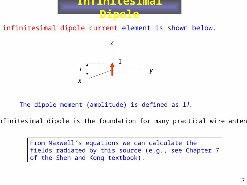
Infinitesimal Dipole
The infinitesimal dipole current element is shown below.
x
y
z
Il
The dipole moment (amplitude) is defined as I l.
From Maxwell’s equations we can calculate the fields radiated by this source (e.g., see Chapter 7 of the Shen and Kong textbook).
The infinitesimal dipole is the foundation for many practical wire antennas.
18
Infinitesimal Dipole (cont.)
0
0
0
0 20
0 20 0
00
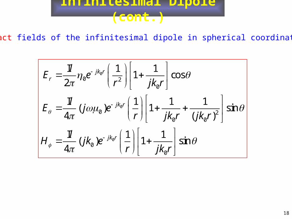
I 1 11 cos
2
I 1 1 1( ) 1 sin
4 ( )
I 1 1( ) 1 sin
4
jk rr
jk r
jk r
lE e
r jk r
lE j e
r jk r jk r
lH jk e
r jk r
The exact fields of the infinitesimal dipole in spherical coordinates are
19
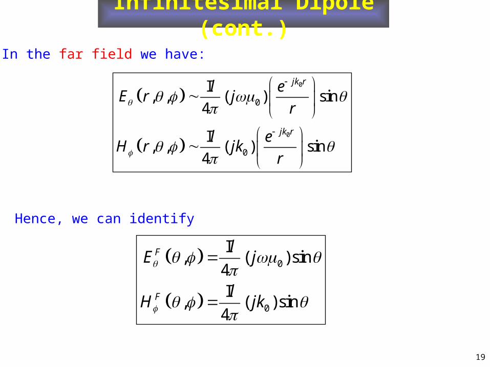
Infinitesimal Dipole (cont.)
0
0
0
0
I, , ( ) sin
4
I, , ( ) sin
4
jk r
jk r
l eE r j
r
l eH r jk
r
In the far field we have:
0
0
I, ( )sin
4I
, ( )sin4
F
F
lE j
lH jk
Hence, we can identify
20
Infinitesimal Dipole (cont.)
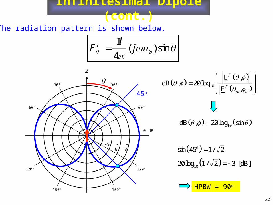
The radiation pattern is shown below.
0
I( )sin
4F l
E j
10
E ,dB , 20log
E ,
F
Fm m
10dB , 20log sin
HPBW = 90o
10
sin 45 1 / 2
20log 1 / 2 3 [dB]
o
-9 -3 -6
0 dB
30°30°
60°
120°
150° 150°
120°
60°
z
45o
21
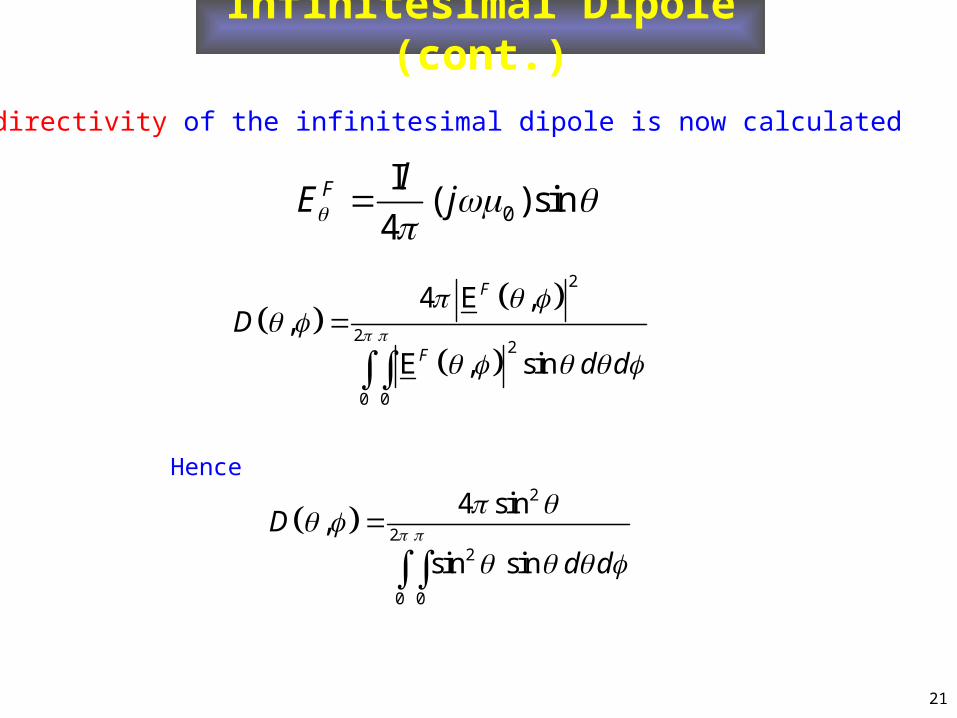
Infinitesimal Dipole (cont.)
The directivity of the infinitesimal dipole is now calculated
0
I( )sin
4F l
E j
2
22
0 0
4 E ,,
E , sin
F
F
D
d d
2
22
0 0
4 sin,
sin sin
D
d d
Hence
22
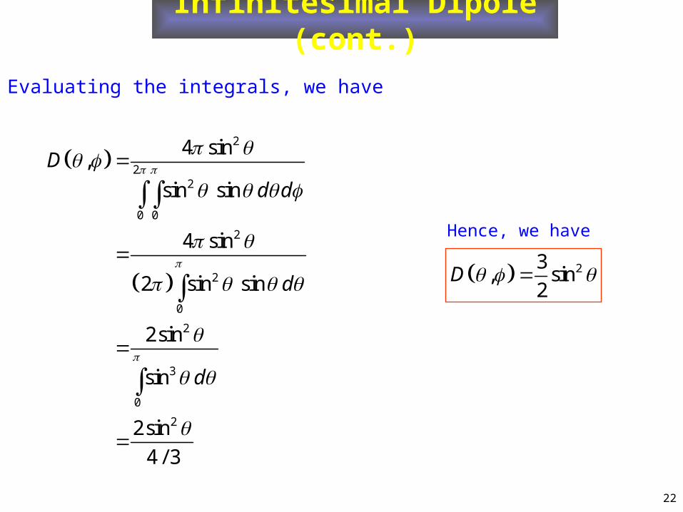
Infinitesimal Dipole (cont.)
Evaluating the integrals, we have
2
22
0 0
2
2
0
2
3
0
2
4 sin,
sin sin
4 sin
2 sin sin
2sin
sin
2sin
4 / 3
D
d d
d
d
Hence, we have
23, sin
2D
23
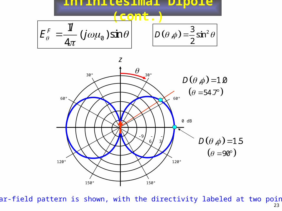
Infinitesimal Dipole (cont.)
23, sin
2D
, 1.5D
, 1.0D o54.7
0
I( )sin
4F l
E j
The far-field pattern is shown, with the directivity labeled at two points.
o90
-9 -3 -6
0 dB
30°30°
60°
120°
150° 150°
120°
60°
z
24
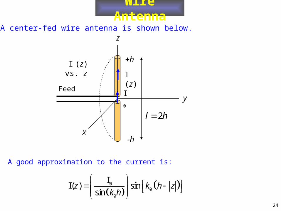
Wire Antenna
00
0
II( ) sin
sinz k h z
k h
A good approximation to the current is:
A center-fed wire antenna is shown below.
y
+h
z
I (z)
x-h
Feed
2l h
I 0
I (z) vs. z
25
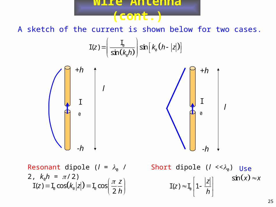
Wire Antenna (cont.)
00
0
II( ) sin
sinz k h z
k h
A sketch of the current is shown below for two cases.
Resonant dipole (l = 0 / 2, k0h = / 2) Short dipole (l <<0)
0I( ) I 1z
zh
0 0 0I( ) I cos I cos
2
zz k z
h
+h
-h
lI 0
+h
-h
l
I 0
sin x xUse
26
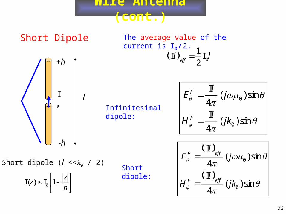
Short Dipole
Short dipole (l <<0 / 2)
0I( ) I 1z
zh
Wire Antenna (cont.)
The average value of the current is I0 / 2.
0
1I I
2effl l
0
0
I( )sin
4I
( )sin4
effF
effF
lE j
lH jk
Infinitesimal dipole:0
0
I( )sin
4I
( )sin4
F
F
lE j
lH jk
Short dipole:
+h
-h
lI 0
27
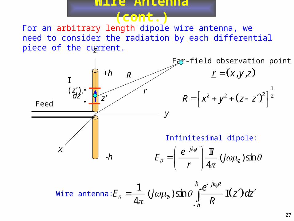
Wire Antenna (cont.)For an arbitrary length dipole wire antenna, we need to consider the radiation by each differential piece of the current.
Far-field observation point
, ,r x y z
0
0
I( )sin
4
jk re lE j
r
0
0
1( )sin I
4
h jk R
h
eE j z dz
R
Wire antenna:
Infinitesimal dipole:
1
22 2 2R x y z z y
+h
z
x-h
Feed
r
R
dz' z'
I (z')
28
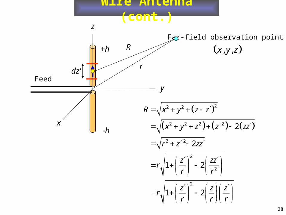
Wire Antenna (cont.)
Far-field observation point
z
y
+h
x-h
Feed
r
R
dz'
22 2
2 2 2 2
2 2
2
2
2
2
2
1 2
1 2
R x y z z
x y z z zz
r z zz
z zzr
r r
z z zr
r r r
, ,x y z
29
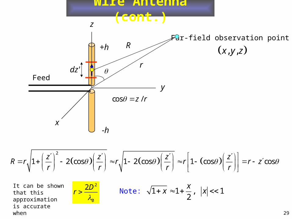
Wire Antenna (cont.)
Far-field observation point
2
1 2 cos 1 2 cos 1 cos cosz z z z
R r r r r zr r r r
, ,x y z
1 1 , 12
xx x Note:
z
y
+h
x-h
Feed
r
R
dz'
cos /z r
2
0
2Dr
It can be shown that this approximation is accurate when
30
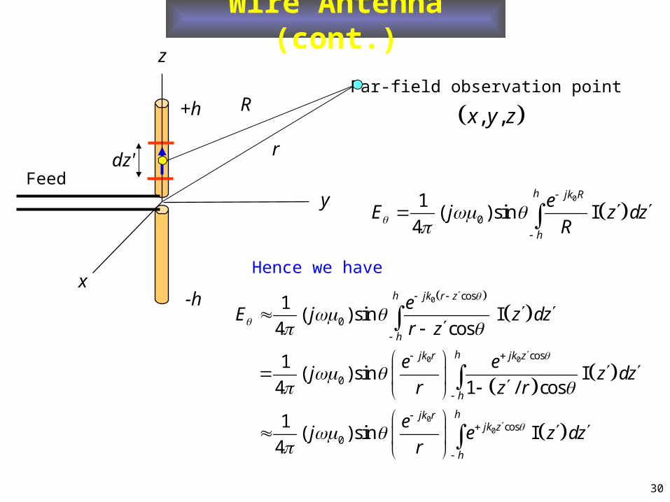
Wire Antenna (cont.)
Far-field observation point
z
y
+h
x-h
Feed
r
R
dz'
, ,x y z
0
0 0
0
0
cos
0
cos
0
cos0
1( )sin I
4 cos
1( )sin I
4 1 / cos
1( )sin I
4
h jk r z
h
hjk r jk z
h
hjk rjk z
h
eE j z dz
r z
e ej z dz
r z r
ej e z dz
r
0
0
1( )sin I
4
h jk R
h
eE j z dz
R
Hence we have
31
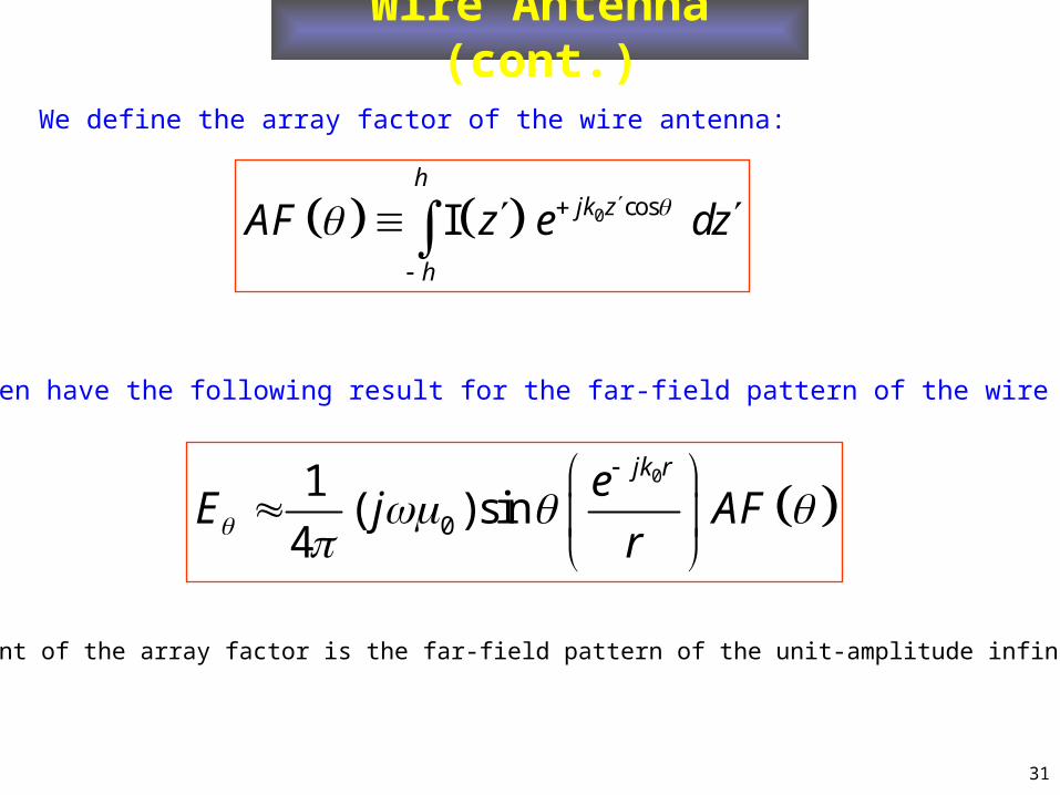
Wire Antenna (cont.)
We define the array factor of the wire antenna:
0 cosIh
jk z
h
AF z e dz
We then have the following result for the far-field pattern of the wire antenna:
0
0
1( )sin
4
jk reE j AF
r
The term in front of the array factor is the far-field pattern of the unit-amplitude infinitesimal dipole.
32
Wire Antenna (cont.)
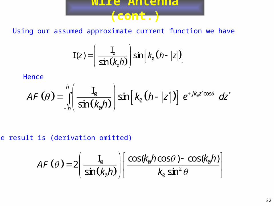
Using our assumed approximate current function we have
0 cos00
0
Isin
sin
hjk z
h
AF k h z e dzk h
The result is (derivation omitted)
0 0 0
20 0
I cos( cos ) cos( )2
sin sin
k h k hAF
k h k
00
0
II( ) sin
sinz k h z
k h
Hence
33
Wire Antenna (cont.)
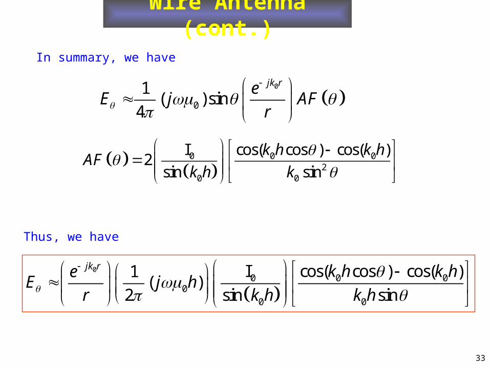
In summary, we have
0 0 0
20 0
I cos( cos ) cos( )2
sin sin
k h k hAF
k h k
0
0
1( )sin
4
jk reE j AF
r
0
0 0 00
0 0
I cos( cos ) cos( )1( )
2 sin sin
jk r k h k heE j h
r k h k h
Thus, we have
34
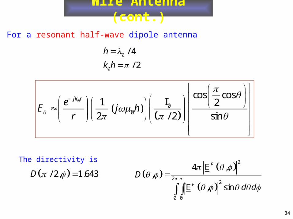
Wire Antenna (cont.)
For a resonant half-wave dipole antenna
0
00
cos cosI1 2
( )2 / 2 sin
jk reE j h
r
0
0
/ 4
/ 2
h
k h
/ 2, 1.643D
The directivity is
2
22
0 0
4 E ,,
E , sin
F
F
D
d d
35
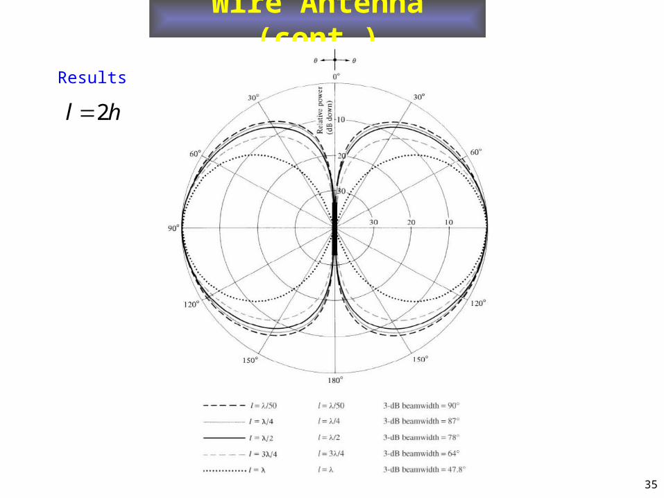
Wire Antenna (cont.)
Results
2l h
36
Wire Antenna (cont.)
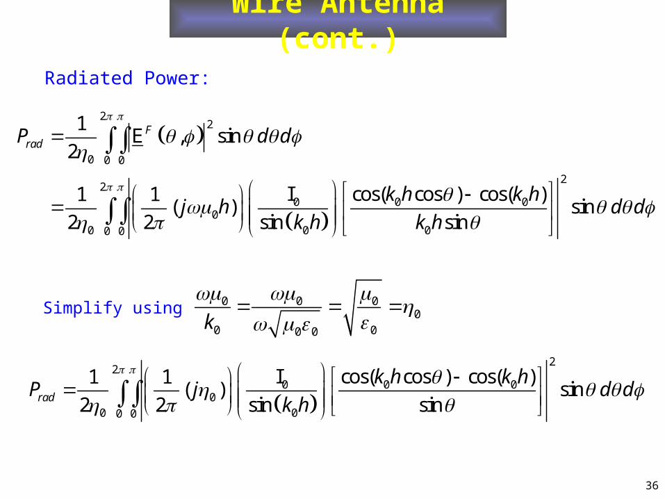
Radiated Power:
22
0 0 0
22
0 0 00
0 0 00 0
1E , sin
2
I cos( cos ) cos( )1 1( ) sin
2 2 sin sin
FradP d d
k h k hj h d d
k h k h
0 0 00
0 00 0k
Simplify using
22
0 0 00
0 00 0
I cos( cos ) cos( )1 1( ) sin
2 2 sin sinrad
k h k hP j d d
k h
37
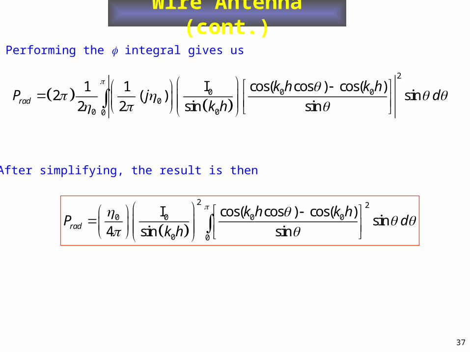
Wire Antenna (cont.)
Performing the integral gives us
2
0 0 00
0 00
I cos( cos ) cos( )1 12 ( ) sin
2 2 sin sinrad
k h k hP j d
k h
2 2
0 0 0 0
0 0
I cos( cos ) cos( )sin
4 sin sinrad
k h k hP d
k h
After simplifying, the result is then
38
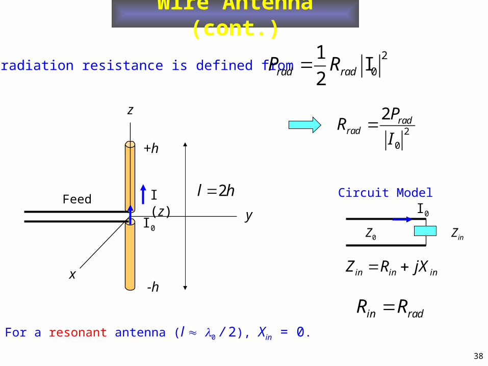
Wire Antenna (cont.)
The radiation resistance is defined from 2
0
1I
2rad radP R
in in inZ R jX
in radR R
Circuit Model
For a resonant antenna (l 0 / 2), Xin = 0.
2
0
2 radrad
PR
I
y
+h
z
I (z)
x-h
Feed2l h
I0 Z0 Zin
I0
39
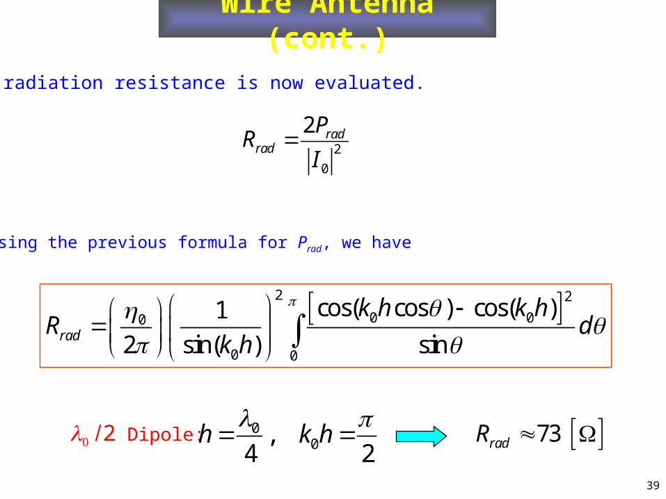
Wire Antenna (cont.)
The radiation resistance is now evaluated.
2
0
2 radrad
PR
I
Using the previous formula for Prad, we have
2 2
0 00
0 0
cos( cos ) cos( )1
2 sin( ) sinrad
k h k hR d
k h
l0 / 2 Dipole: 00,
4 2h k h
73radR
40
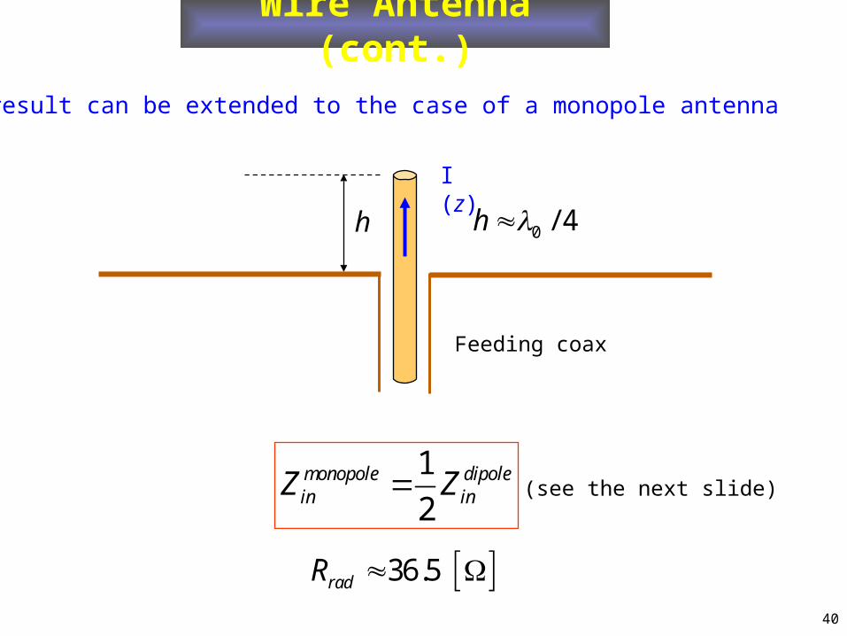
Wire Antenna (cont.)
The result can be extended to the case of a monopole antenna
1
2monopole dipolein inZ Z
36.5radR
(see the next slide)
h
Feeding coax
0 / 4h
I (z)
41
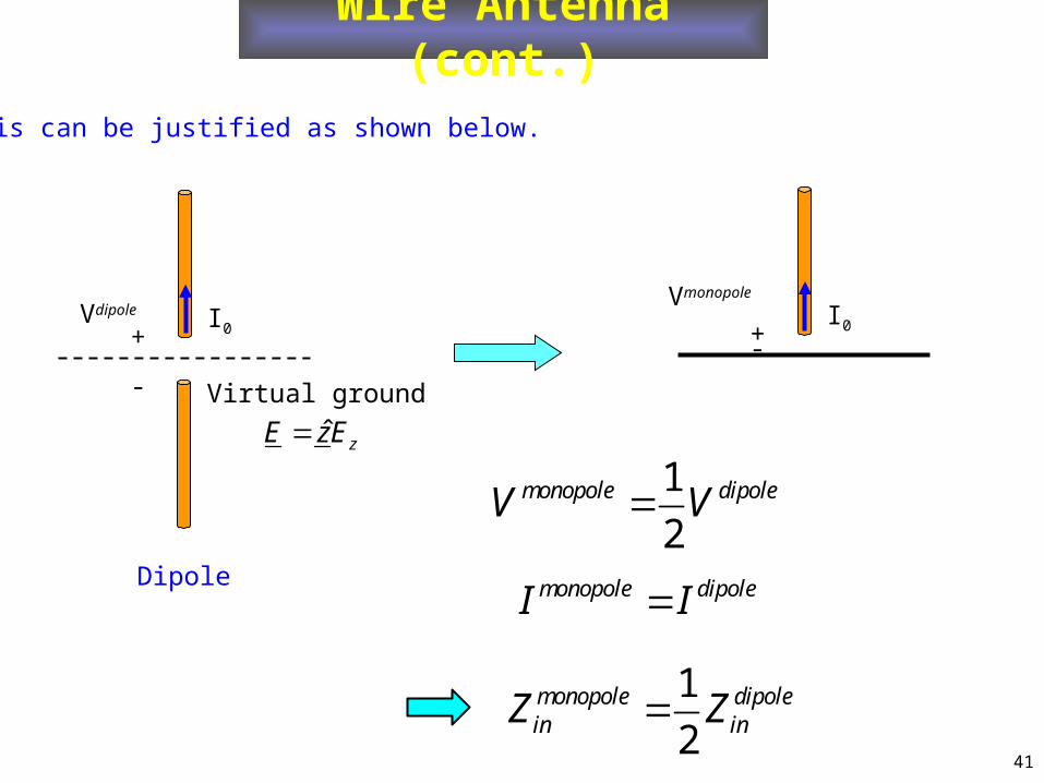
Wire Antenna (cont.)
This can be justified as shown below.
+
-
Dipole
Vdipole I0
Virtual ground
+
Vmonopole
I0
-
1
2monopole dipoleV V
ˆ zE zE
monopole dipoleI I
1
2monopole dipolein inZ Z
42
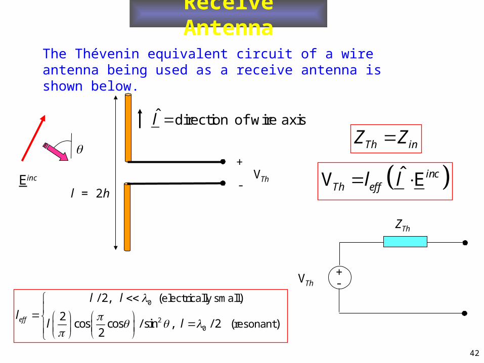
Receive Antenna
The Thévenin equivalent circuit of a wire antenna being used as a receive antenna is shown below.
+-VTh
ZTh
Th inZ Z
ˆV EincTh effl l
0
20
/ 2, ( )
2cos cos / sin , / 2 ( )
2eff
l l
ll l
electrically small
resonant
+
-VThEinc
l = 2h
l̂ direction of wire axis
43
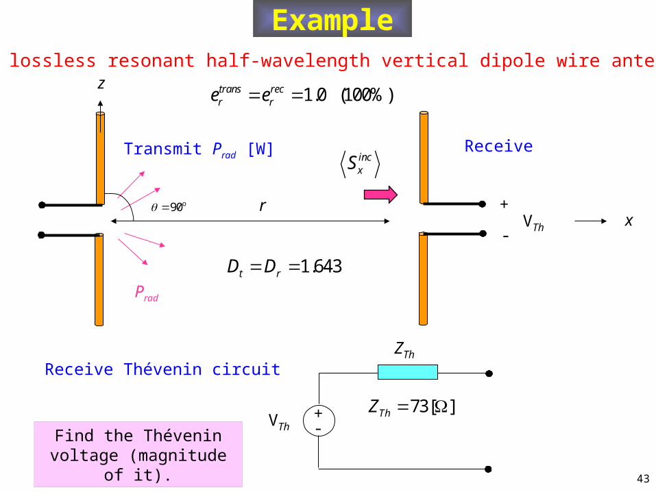
Example
+-VTh
ZTh
Receive Thévenin circuit
Two lossless resonant half-wavelength vertical dipole wire antennas
73[ ]ThZ
1.643t rD D
incxS
+
-VTh
Receive
xr
Transmit Prad [W]
Prad
z
o90
Find the Thévenin voltage (magnitude of it).
1.0 (100%)trans recr re e
44
Example (cont.)
o
2
90
0
2 2 2
2
0 020
2 2cos cos / sin
2
2
1.6434 4 4
EE 2 1.643 2
2 4
eff eff
inc incin rad radx t t x
inczinc inc inc rad
x z x
l l l l
l
P P PS G D S
r r r
PS S
r
002
2V 1.643 2
2 4rad
Th
P
r
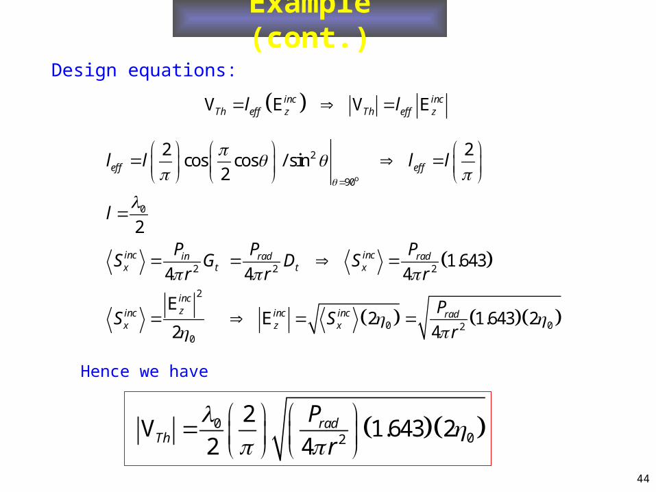
Hence we have
Design equations:
V E V Einc incTh eff z Th eff zl l
45
Example (cont.)
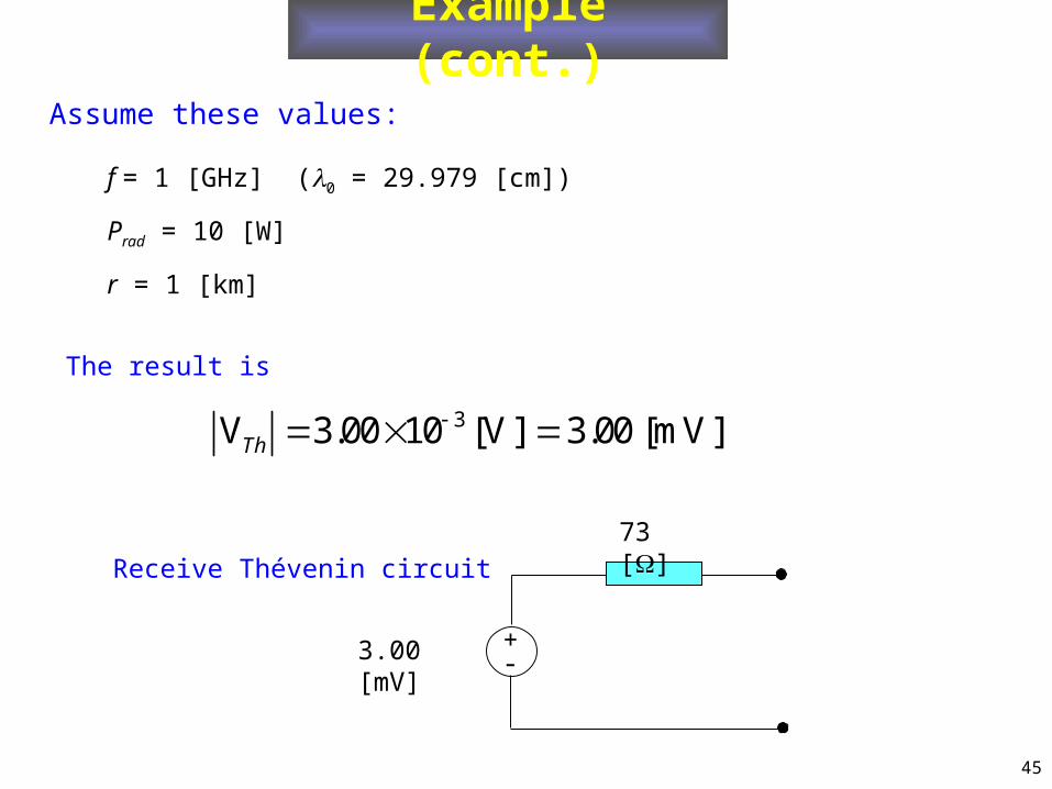
The result is
Assume these values:
f = 1 [GHz] (0 = 29.979 [cm])
Prad = 10 [W]
r = 1 [km]
3V 3.00 10 [V] 3.00 [mV]Th
+-3.00 [mV]
73 []Receive Thévenin circuit
46
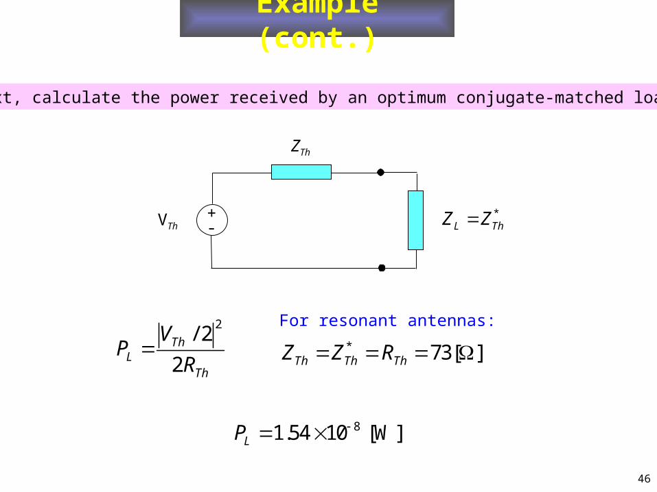
81.54 10 [W]LP
Next, calculate the power received by an optimum conjugate-matched load
Example (cont.)
+-VTh
ZTh
*L ThZ Z
2/ 2
2Th
LTh
VP
R * 73[ ]Th Th ThZ Z R
For resonant antennas:
47
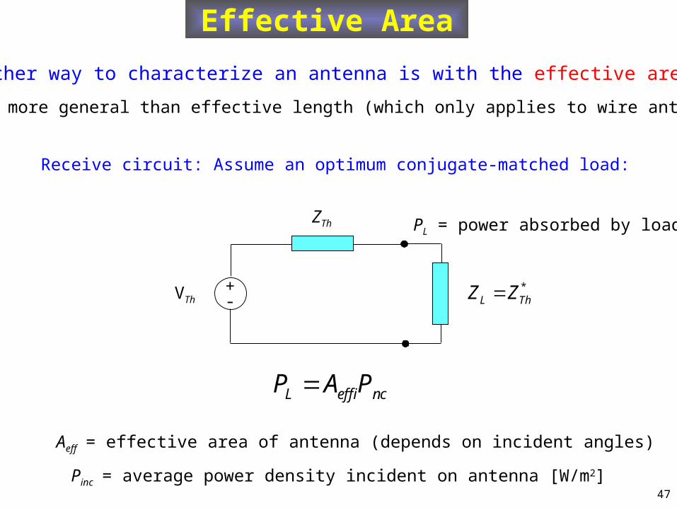
Effective Area
Another way to characterize an antenna is with the effective area.
Receive circuit: Assume an optimum conjugate-matched load:
This is more general than effective length (which only applies to wire antennas).
+-VTh
ZTh
*L ThZ Z
L eff incP A P
Aeff = effective area of antenna (depends on incident angles)
Pinc = average power density incident on antenna [W/m2]
PL = power absorbed by load
48
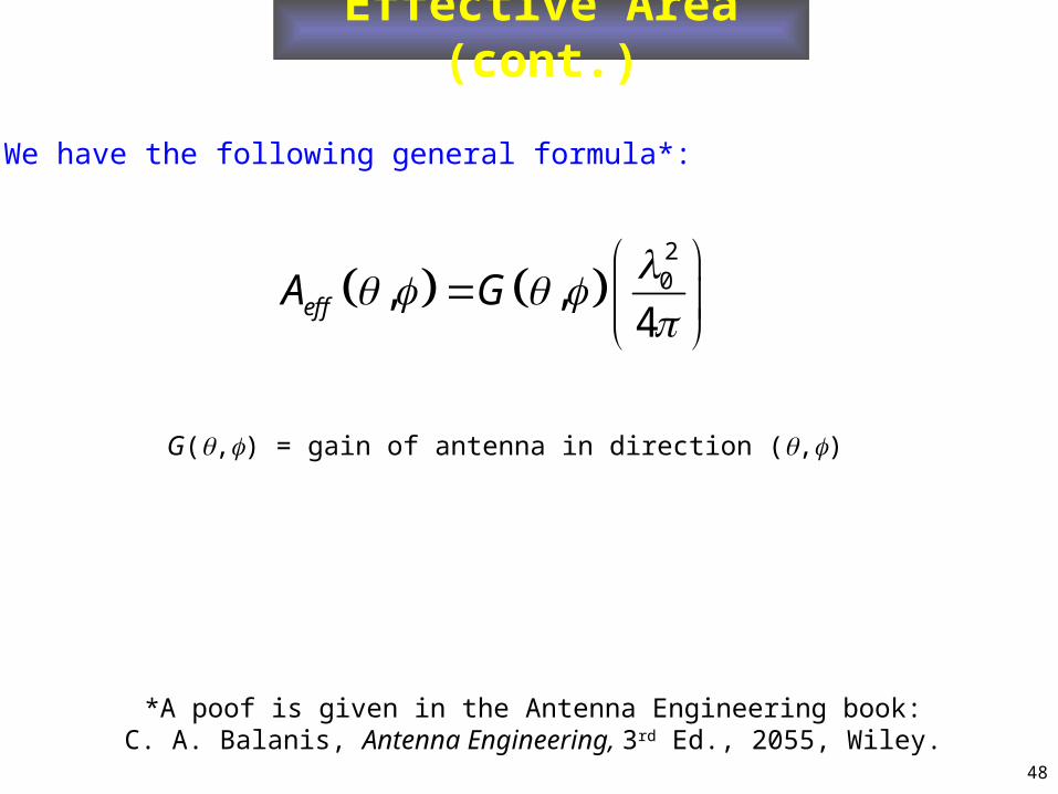
Effective Area (cont.)
We have the following general formula*:
20, ,
4effA G
*A poof is given in the Antenna Engineering book:C. A. Balanis, Antenna Engineering, 3rd Ed., 2055, Wiley.
G(,) = gain of antenna in direction (,)
49
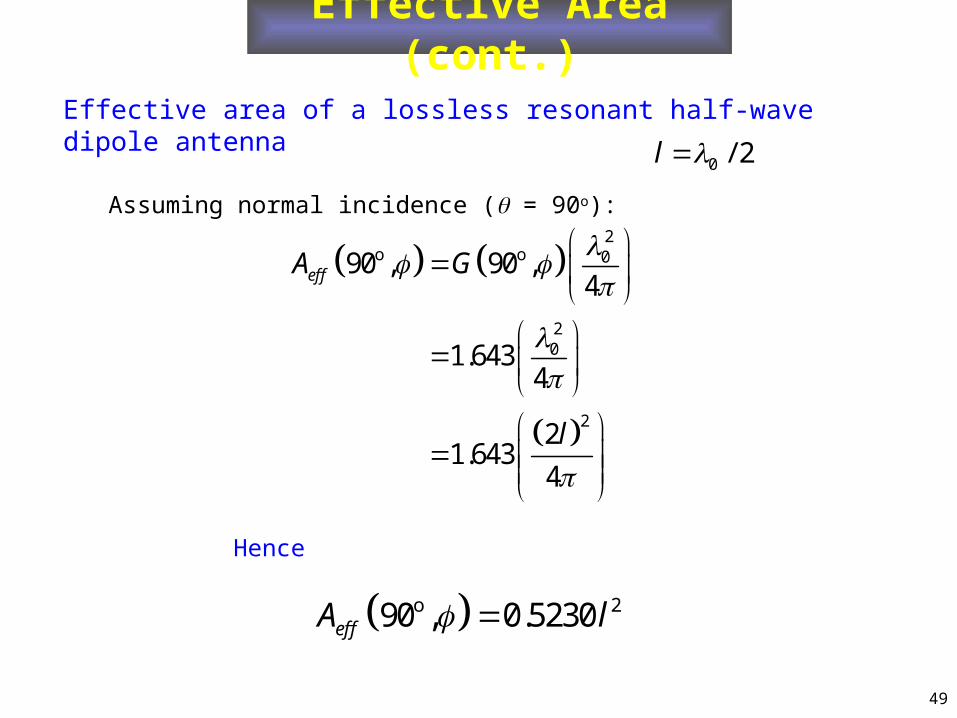
Effective Area (cont.)
2o o 0
20
2
90 , 90 ,4
1.6434
21.643
4
effA G
l
Effective area of a lossless resonant half-wave dipole antenna
o 290 , 0.5230effA l
Hence
Assuming normal incidence ( = 90o):
0 / 2l
50
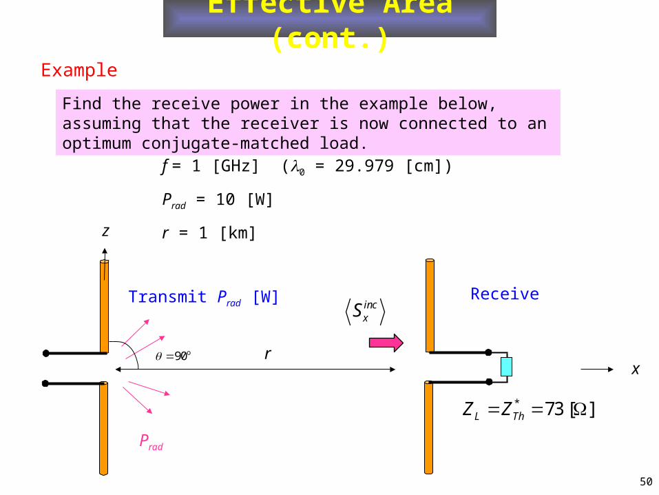
Effective Area (cont.)
Example
Find the receive power in the example below, assuming that the receiver is now connected to an optimum conjugate-matched load.
f = 1 [GHz] (0 = 29.979 [cm])
Prad = 10 [W]
r = 1 [km]
incxS
Receive
xr
Transmit Prad [W]
Prad
z
o90
* 73 [ ]L ThZ Z
51
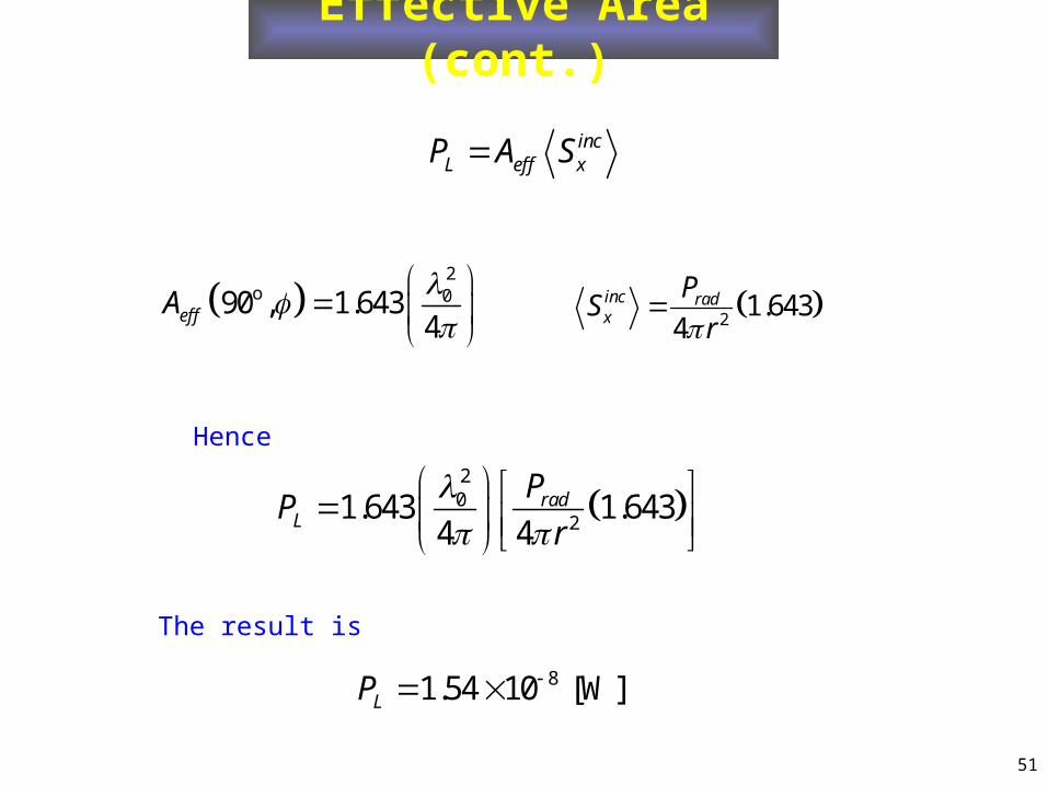
Effective Area (cont.)
2
o 090 , 1.6434effA
incL eff xP A S
21.643
4inc radx
PS
r
20
21.643 1.643
4 4rad
L
PP
r
81.54 10 [W]LP
Hence
The result is
52
Effective Area (cont.)
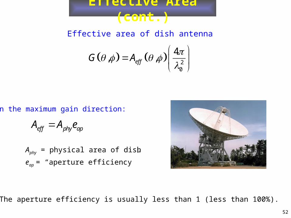
Effective area of dish antenna
20
4, ,effG A
eff phy apA A e
Aphy = physical area of dish
eap = “aperture efficiency”
In the maximum gain direction:
The aperture efficiency is usually less than 1 (less than 100%).