CSLS Conference on the Canada – U.S. Manufacturing Productivity Gap

January 21 - 22, 2000 Château Laurier Hotel, Ottawa, Ontario

Centre for theStudy of Living Standards

Centre d'étude desniveaux de vie

Productivity Growth and Trade Specialization

Rick HarrisSimon Fraser University

Samer KherfiSimon Fraser University

Session 6 “Do Trade Specialization Patterns Contribute to the Gap?”January 22 10:15 AM - 11:45 AM

0

Productivity Growth and Trade Specialization

by

Richard G. HarrisSimon Fraser University and Canadian Institute for Advanced Research

and

Samer KherfiSimon Fraser University

Paper prepared for Centre for the Study of Living Standards

Conference

The Canada-U.S. Manufacturing Productivity Gap

January 21-22

Ottawa, CanadaPreliminary Only

*Comments welcome. Please do not quote without permission. Authors can be reached

by email at rharris@sfu.ca and skherfi@sfuc.ca.

1

1. Introduction

The productivity panic in Canada continues unabated with little resolution yet as

to what the major proximate causes of the decline in Canadian living standards might be

attributed. The long standing gap in Canada-U.S productivity levels remains a continuing

puzzle which thus far has defied a single coherent explanation. Andrew Sharpe in his

overview paper covers a number of the potential explanations. This paper focuses on the

class of explanations which are primarily motivated by the role of international trade as it

relates to manufacturing and productivity growth rates between countries. Now it is

entirely possible that the 'reasons' for the gap have nothing to do with trade per se. Other

explanations may ultimately prove to be more compelling. However the interaction

between trade and productivity growth has historically been important, and in the

Canada-U.S. case the substantial growth in trade volumes in the last two decades strongly

suggests that the two trends might be related.

Why should one focus on explanations related to trade in particular?

There are at least three reasons why trade and trade patterns are potentially important

explanations of the gap. First, trade breaks the direct link between productivity and real

incomes that holds in closed economy models. Two, Canada-U.S. trade volumes are

amongst the largest in the world, and Canada is heavily specialized by region in its trade

with the United States1. Close to 90 percent of Canadian manufacturing exports go to the

United States. The growth in trade and openness vis-a-vis the U.S. has been nothing

short of phenomenal in the 90's with export to GDP ratios going from the 25 percent

range to the 40 percent range in a decade. The well documented convergence effect

should have been working in Canada's favor--with Canada catching-up to the US after the

implementation of the FTA/NAFTA, but this does not appear to be the case. Third, the

increased trade and factor mobility, including the mobility of knowledge, has raised the

counterfactual question as to how North American regional specialization is likely to

evolve and where the Canadian regions might fit in that broader pattern.

1 See Grady and MacMillan(1998).

2

Even within the class of 'trade explanations' the analyst is confronted with a

serious problem in sorting out measurement issues , competing hypotheses, causality

versus correlation, and data constraints. This paper is an attempt to sort out some aspects

of this puzzle. Ideally one would like to have a tight theoretical framework in which to

conduct the data analysis. Part of the problem however is that different theories of trade

suggest different interpretations, and ourpurpose here is not to test a particular trade

theory. It is useful thought to review briefly what two major trade theories, an amended

version of Heckscher-Ohlin for productivity differences, and the Ricardian trade model,

have to say about changes in productivity and trade. The paper then goes on to look at

the productivity growth process in Canadian manufacturing and its interaction with trade.

Again here there are many alternative theories of endogenous productivity change which

have been advanced in the last decade ( Grossman and Helpman(1991) ) which suggest

different causal linkages between trade and productivity growth. The most famous of

these is Baumol's convergence hypothesis, and empirically there is a fairly strong

aggregate evidence for conditional convergence which tends to be faster the greater the

degree of openness.

A trade explanation for the Canada-U.S. gap in productivity levels, or the

persistence of the gap, could arise in at least two different ways. Think of a general

model with a two way linkage running between trade and productivity growth.

Productivity patterns influence trade patterns through comparative advantage effects, and

trade influences productivity growth through a variety of endogenous growth

mechanisms. Both trade specialization and productivity change over time as a

consequence of long lived investment decisions by governments and firms. Moreover

policy and luck can have a significant influence on how a country specializes and the

success of attempts to invest in productivity improvements. Ex post a gap can increase or

persist for two quite different reasons.

a. The pattern of investments in specialization turn out to be inconsistent

with the sectors/industries in which productivity improvements are most

successful.

b. The pattern of productivity improvements are not in those areas which

have the highest rates of growth in demand in external markets. a f

3

The first hypothesis suggests that for some reasons the economy tended to

allocate resources towards the sectors which had lower productivity potential. The

second set of reasons suggests that the productivity growth process itself has been in the

wrong direction, or at least inconsistent with external developments. It should be

recognized that in both cases we are looking for plausible ex post rationalizations for the

gap. It is important to remember that Canada's poor productivity performance is hardly

novel among the OCED countries. For other countries that have been low on the

productivity pole, for e.g. Norway, Australia and the United Kingdom, similar concerns

have been expressed. For many years U. S. productivity growth lagged European growth

rates and it is only the more recent years which show signs of a significant acceleration of

U.S. productivity growth. Owever explanations which may be valid in each of those

cases may not be valid in the case of the Canada-U.S. comparison.

2. Productivity and Trade Theories.

In this section I want to review two major trade theories and discuss how

international productivity differences are manifested in trade patterns, and how

productivity growth and levels are affected by trade. The two main theories are a) the

Hecksher-Ohlin framework amend to incorporate neutral productivity differences. And

b) the Ricardian and other models of trade specialization.

2. a) Heckscher-Ohlin with Neutral Productivity Differences.

This set of theories is most closely related to the various measurement

frameworks which emphasize TFP accounting at the sectoral level, and PPP adjustments

for constructing comparable real output levels comparisons. It would be reasonable to

claim that the bulk of the measurement literature falls within this framework. To keep

matters simple think of a two country framework. The Home country (Canada)

corresponds to the variables without an * and the US variables will be denoted by an *.

We ignore third countries.2 There are n homogenous tradable goods, trading under

2 In the case of the smaller country Canada who is assumed to be a price taker in world goods markets in

this theory, ignoring third country issues is not that important.

4

conditions of non-distorted free trade at prices Pi. Each good i can be thought of a

produced under competitive classical constant returns conditions with output Yi of good i

the home and foreign country are given by

*)M*,L*,K(*F*A*Y

)M,L,K(FAY

iiiiii

iiiiii

=

=

where the inputs are capital labour and materials. The materials input Mi a sub-

aggregate of the n traded goods. The Hicks neutral productivity differences are the terms

Ai One can disaggregate capital and labour and quality adjust. Trade is explained both

by productivity differences A/A* and by factor endowment differences K/K* etc.

Countries tend to export goods which are intensive in the use of their abundant factor and

goods in which they have a comparative advantage as measured by Ai/Ai*. Factor prices

in equilibrium reflect average productivity differences between countries.

The substitution aspects of the technology as summarized in the functions Fi and

Fi* are usually taken as similar across countries. If both the Fi and Ai are different across

countries, then the H-O-V model of trade does not have an predictive content. In any

case provided one can measure either growth rates of TFP or do levels comparisons

provided are outputs and inputs can be measured in comparable units across countries.

The HOV model without specialization assumes all goods are produced in all

countries. This is usually implemented at the 2 or 3 digit industry level with an explicit

assumption that the steel industry in Canada, for example, is producing a homogeneous

output which is the same as that produced in the United States. This allows meaningful

comparison of both average labor productivity, ALP, and TFP across the same sectors.

The HOV framework automatically both suggests and constrains the manner in which the

productivity trade question is framed.

Real incomes, the gap and terms of trade effects

Most Canadian economists are familiar with this model. Canada is usually treated

as a small open economy. If we think of manufacturing as one large sector with

resources K and L available, the production sector equilibrium can be represented by the

manufacturing GDP function

5

==== ∑ ∑∑)i i

ii

iiiiiiiiy,l,k LL;KK);L,K(FAY:Ypmax)L,K,A,p(G

where p is the vector of internationally determined goods prices. If we normalize GDP

say by dividing by the number of workers L in each country relative GDP per worker

(v/v*) is measured by

*L/*)L*,K*,A,p(GL/)L,K,A,p(G*v/v = .

Changes in productivity holding all else constant will change the gap. In fact the change

in manufacturing GDP due to a change in the productivity of sector i TFP Ai alone is

given by

iiAsv =

where si is the value share of sector i's output in total manufacturing output, and hats

denote percentage changes. The change in the total gap reflects therefore the growth

rates of the TFP's in both countries and the relative output shares in each country.

In this amended HOV model with productivity differences the gap for a small

open economy is either due to factor endowment differences, or to TFP differences. Note

that the theory is dependent only on international prices, p and supply side effects of

technology or resources. Over time as the PPF's of the two economies shift out in theory

competitive markets will choose the GDP maximizing resource allocation given the

evolution of exogenous productivity patterns. In practice however economies do not

costlessly and instantly change sectoral patterns of specialization. Large investments are

required in both physical and human capital for this to occur. Moreover taxes, subsidies,

and other economic policies can affect this resource allocation. Ex post therefore we can

ask whether the revealed pattern of specialization is consistent with one predicted by the

theory--that is did specialization occur in sectors with the highest productivity growth and

most advantageous terms of trade shifts?

2.b Ricardian International Specialization

An alternative to the Heckscher-Ohlin framework and one with quite different

implications resides in the famous Ricardian model of trade in which economies

specialize through trade in different goods. International specialization implies that the

6

set of goods across which comparisons are made are increasingly disparate--that is they

involve comparing apples and oranges. Or to put it more specifically a steel plant in

Hamilton may be producing a different set of products than a steel plant in Buffalo and

thus productivity comparisons are not easily made or in fact even possible. Countries

will differ in aggregate productivity levels depending upon how one weights the different

outputs each country produces. More generally this approach suggests the following:

• One, as production becomes internationally specialized the real growth effects

of productivity change will be increasingly transmitted through terms of trade

changes in the short to medium term, and over the longer term in changes in

the particular pattern of specialization.

• Two, relative real income levels are ultimately dependent upon the pattern of

specialization. A country will tend to have a higher relative income the larger

the share of global spending on manufactures that fall on its goods.

Productivity is important because is determines which goods a nation

specializes in.

As the Ricardian trade theory fallen out of style in recent years it may be useful to review

its productivity implications. To do this we lay out a simple three good, two country

model.

A Ricardian Model of Productivity Growth

In this section a simple two country version of trade and specialization is

reviewed. The model is quite traditional except for the introduction of a non-traded good

in each country (good 1) to add a necessary dose of realism, and one quite important from

the perspective of interpreting measurement exercises. There are two trade goods (2 and

3) and two countries Home and Foreign. The Foreign country is denoted by a *

superscript on most variables. What is slightly novel is that we shall focus on an

equilibrium with international specialization, and secondly one which is in steady-state

growth equilibrium but with exogenous productivity growth across all activities.

Output of each good i is denoted by Yi and a value added input aggregator whose

quantity is denoted by Li and whose nominal factor price is W. Hence forth this factor

will simply be called 'labour'. Factors are mobile between sectors but not countries. Each

sector has a constant returns production function

7

321 ,,iLiii == ΑΥ

In equilibrium with competition goods price Pi and the economy wide factor price is

given by

W1

ii Α

=Ρ

The growth rate of any particular variable will be hatted ie ^. The growth rate of rate of

average labour productivity in sector i is denoted by gi so that

ii g=Α

Labour market clearing requires that the inelastically supplied labour endowment

L equals labour supply to each sector; 321 LLLL ++= . To keep things simple assume

Mill-Cobb-Douglas preferences on the part of all consumers with expenditure shares αi.

Demand for each good i is then given by

LAPWL

D iii

ii α

α==

and supply is given by

iii LAS =

In autarky market clearing implies that labour is allocated according to the rule

LL iai α=

Real income (as calculate by the indirect utility function of the representative Mill

consumer) is denoted by U and

321

321321 321

321

321

ααααααααα AALA

AW

AW

AW

WLPPP

IU =

==

The growth of real income will be denoted by y--this is what we would conventionally

think of as the appropriate index of the change in living standards if we hold L fixed.

Assume there are no issues of labour force participation or hours worked. For the most

part we will stick with this interpretation. In general with increases in L the aggregate

change in real income is given by

332211 gggLUlogdy ααα +++=≡

The important point here is that in a closed economy the aggregate change in living

8

standards is given by the weighted sum of productivity growth rates in each of the three

sectors with weights corresponding to expenditures shares.

International Trade and Specialization

We now introduce trade between the two countries. We shall use the convention

of taking tothe price of non-traded goods in the foreign country as the numeraire. (You

can think of this as simply US dollars to measure all values in). With this normalization

wages in Foreign are simply equal to productivity in the non-traded sector in foreign, so

that *1

*1 *1 AWPSet =⇒= .

We now want to concentrate on an equilibrium in which both countries are specialized.

As the number of goods becomes large this will be the 'normal case'. Country size is

reflected in the number of goods each country is specialized in. Assume therefore that

Home is specialized in good 2 and Foreign in good 3. This will require that in

equilibrium the unit cost of producing good 2 is no greater in Home than in Foreign, and

conversely for good 3. Hence it must be the case that

*33

*22

2*1*1

AWW

Aand

AWW

Ac ≥≤=

Together these imply the following comparative productivity inequalities which imply

that Home has a relative productivity advantage in good 2 and Foreign in good 3;

2

3*2

*3

AA

AA

≥

A number of important and interesting implications follow from this simple model. First

relative wages (the factoral terms of trade) reflect taste and aggregate endowments--not

relative productivities/

=3

2** α

αL

LWW .

Real income growth in Home and Foreign (lower case y ) is given by the equations

*332211

logggg

udyααα ++=

=

*3322

*11

* *logggg

udyααα ++=

=

9

This equation illustrates a simple and important result. Real income growth is

identical in the two countries provided productivity growth is the same in both countries

non-traded sectors. Thinking of manufacturing as 'traded goods';this implies that

differential rates of growth of productivity in manufacturing do not lead to differential

rates of growth in real income. Why? Real income growth and GDP growth diverge

however in this framework due to the presence of terms of trade effects. Real GDP

growth calculated as the weighted average growth rates of sectoral growth, with the

weights corresponding to value of output weights. In equilibrium the value share of

output devoted to sector 1 is in fact constant since

111111 LALAY α==

( ) LAY 212 1 α−=

and thus

1

11

1

2211

111 α

α==

+≡

WL

LAAW

YPYPYPS

The growth rate of real GDP in Home is given by

( ) 2111 1 ggr αα −+≡

The difference between growth rates of real income and GDP in Home are given by

( )

( ) ( )23333212

2111332211

g*g*gg1

g1g*gggry

−α=α+−α+α=

α−−α−α+α+α=−

The implications of this equation are that real income and real GDP growth will diverge

to the extent that growth rates of productivity of the goods in which each country has

specialized have diverged. In particular has Home has specialized in good 2, if

productivity growth in Home industry 2 proceeds at a faster pace than productivity

growth in Foreign's exports sector 3, Home will have GDP growth which is faster than

real income growth. Real output gains on the GDP side are more than offset by terms of

trade losses. The argument is completely symmetric and the opposite would hold for

foreign.

Simple levels comparisons on productivity in a model with complete

specialization could try to measure of A2/A3. It should be clear that in this model the

10

actual value of these relative productivities are not directly related to the relative real

incomes. Indeed this ratio (the 'gap') could diverge or converge and have no impact on

relative real incomes. The real income in each country is the Wage divided by the cost of

living index dual to the Cobb-Douglas utility function. This v and v* denote real income

levels per unit labour in Home and Foreign. In a free trade equilibrium we have that the

ratio of real value added (or real income) per unit of composite factor is given by

1))((** *

1

1

3

2 α

αα

AA

LL

vv =

Note that relative real incomes reflect the demand side of the model. In particular

the ratio of expenditure shares on the goods in which each country has specialized affect

relative real incomes. Holding productivity in services constant a country tends to be

relatively better off--that is it has a higher relative real income to the extent a larger share

of expenditures on manufactures falls on its manufacturing sector. Furthermore if

expenditure shares change over time, a country specialized in a good with a growing

expenditure share will tend to have a rising relative income. Productivity affects the gap,

as measure by v/v*, only to the extent that it affects the patterns of specialization.

To address the question of changes in the patterns of specialization would really needs a

dynamic model. In the short run it is useful to think of the pattern of specialization as

being fixed and only changing slowly. This simple model can be generalized in a number

of ways. In fact there are a variety of trade theories which hinge on some combination of

scale economies at the level of the firm or plant, and either vertical or horizontal product

differentiation which give rise to similar results. The important point to emphasize is that

unlike the HOV model the demand side matters. A country that is specialized in a good

with a high growth in demand will experience a rising real income level. Demand might

shift in favor of one country because it develops new goods which the other country does

not. Observed real income growth therefore reflects a combination of productivity

changes on existing goods which are transmitted abroad through terms of trade changes,

and real income increases due to the development of new goods or industries in the

country in question has a comparative advantage.

11

3. The Dynamics of Productivity Growth

How does trade interact with productivity growth? In the HOV model

productivity differences will have effects which tend to bias growth in favor of high

growth sectors, given unchanged terms of trade. In the Ricardian model productivity

growth will tend to shift specialization patterns towards sectors in which the country

achieves comparative advantage (assuming policy allows this to happen). Much of the

endogenous growth literature has been summarized in terms of the openness and

convergence hypothesis which can be viewed as a reduced form specification of

productivity dynamics consistent with either the Ricardian or HOV model an dsome

unspecified process generating technological change both at Home and internationally.

1. Most of the explanations of why productivity differs tend to go strictly

speaking beyond either the HOV or Ricardian framework, but the bulk of the

literature tends to focus on national specific explanations.

2. Two of the most important explanations relating productivity growth to

openness and trade have been a)the conditional convergence hypothesis.

Countries with the lower TFP levels will tend, ceteris paribus to have

productivity growth rates which are higher, and b) the spillovers approach

which suggests that trade and foreign direct investment are important

mediators of the transmission of technical change across counties. The latter

is discussed by Jeff Bernstein at this conference.3

A typical convergence equation for productivity growth looks like

ii

iiii Z)

*A*AA

(A γ+−

λ+α=

Various theories offer different explanations for the determinants of the sector-country

specific rates of technological change, and for the rate of convergence s λ as a function of

the productivity gap. The set of variables Z may a number of other productivity growth

drivers depending upon which endogenous growth theory is appealed to. Strictly

speaking this equation is probably best viewed as a reduced form rather than a structural

3 See also Bernstein(1996).

12

equation. It has been applied most frequently in the case of national economies, but there

is now a growing literature which uses panel data for manufacturing industries to test for

similar effects.

The issue of whether connditional-β convergence occurs in the manufacturing

sector is far from resolved. There are a number of studies which document the non-

convergence in measured productivity of the manufacturing sector industrial counties, a

trend which began in the mid 1980's, after three decades of almost continuous

convergence. The general convergence hypothesis seems to describe aggregate GDP

OECD data fairly well and there is a large literature on this issue. At the sectoral level

however there appears to have been an increase in dispersion of manufacturing

productivity levels at least since the mid 1980's. Bernard and Jones(1996) report that

substantial reductions in the β conditional convergence parameter suing average labour

productivity data from the period 1970-1987 (β=-0.032) relative to the period 1975-87(

β=-0.0275.) but in both cases are insignificant. The ratio between the least productive

and most productive was 1.96 in 1987 and is at least as high as in 1975 using a variety of

measures of productivity. More recent data using the OECD ISDB data show that as of

1996 the situation has changed little with substantial divergence between the leader

country (the US) and all other countries on labour productivity. As is well known

Canada using these measures Canada converged through the late 80's and subsequently

has fallen behind the US substantially.4

There is now a large theoretical literature which argues that 'openness' affects

productivity dynamics through a variety of channels. In the endogenous growth literature

knowledge drives growth and openness will affect growth to the extent that its affects

incentives to innovate, the underlying productivity of innovation or the transmission of

research discoveries across national borders. One can classify these effects to the extent

they effect (a) the rate of technological progress which is independent of the stock of

ideas abroad , (b) the rate at which knowledge diffuses across international borders , and

(c) the available stock of knowledge available internationally. Quantitatively an

4 Specifically the OCED reports using value added per hour worked that Canada in 1985 stood at 85

percent of the US level and in 1996 was at 69 percent of the US level.

13

important question is whether openness has a more important effect on α or λ. The

former or spillovers approach may reflect general spillovers associated with trade and

Foreign Direct Investment while the latter 'convergence effect' bears directly on the

technology which is available abroad and whom the trading partners are. In the case of

Canada, a sudden forging ahead by the U.S. would be ultimately good news if the most

important effect of openness is on the rate of convergence. However the absence of

convergence of manufacturing productivity levels is the international analogue of the

Canada-US gap problem. Is the convergence hypothesis incorrect or is something else at

work?

In the case of nation specific explanations one looks for common national

determinants of either the α or λ parameters. This can be applied fairly naturally in the

HOV framework. One may also be interested however in sectoral differences in

productivity growth--in particular is productivity growth concentrated in particular

sectors due to differences in either openness or other variables?

A natural question to ask is whether productivity growth is forward looking. This

makes sense as investments are required to produce productivity growth. Thus one could

include under the list of Z factors which affect investments in productivity. Under the

HOV framework it is natural to ask whether productivity growth has been concentrated in

sectors with favorable terms of trade developments. In the Ricardian model demand

variables could be important. That is did productivity growth occur in sectors with good

growth in external demand, measured for example by either exports or other proxies for

foreign demand?

4. Measuring Specialization

One prior question to ask is whether there is any evidence that specialization is

becoming relatively more important as the Canadian economy has opened up to trade

with the United States over the past two decades. There are a number of ways to do this.

At a broad inter-industry level looking at industry importance by the share of value added

the Canadian manufacturing structure remains remarkably stable. See table 1. The top

10 sector from 1988 to 1995 increased their share of total value from 46 percent to 50

14

percent. But once you get below the top two, Transportation Equipment and Pulp and

Paper you get remarkably little variation over the period.

What about trade? First let's examine some traditional aggregate indexes of inter

versus intro industry trade reported in Table 2. G, N and Z are the conventional indexes

of gross, inter-industry and intra-industry trade (IIT index) on a bilateral basis. G is the

sum of N and Z.5 There have been substantial increases in intra-industry trade between

Canada and the United States, but also in gross international specialization and inter-

industry trade. The IIT index is conventionally taken as an indicator of increased

horizontal specialization. At the level of individual sectors there are some sectors that

have had substantial increases in intra-industry trade as reported in Table 3. Note that

many of these industries are either intermediate or capital goods industries. This leads to

the question of whether the specialization that is going on is primarily vertical or

horizontal. It could be either but a number of studies for the EU suggest the pattern of

specialization emerging there is primarily vertical.

5 Fuentes-Godoy et al. (1996) provides a useful discussion of the use of trade specialization indexes.

15

Table 1

Top 10 Manufacturing Industries by Share of Value Added of Total Manufacturing

1988 and 1995

Top 10 1988 rank share Top 10 1995 shareTRANSPORTATION EQUIPMENT IND. 1 13.17 TRANSPORTATION EQUIPMENT IND. 16.154

PULP & PAPER INDUSTRIES 2 9.018 PULP & PAPER INDUSTRIES 10.019INDUSTRIAL CHEMICALS INDUSTRIES 3 3.57 ELECTRONIC EQUIPMENT INDUSTRIES 4.12NON-FERROUS SMELTING & REFINING 4 3.484 OTHER MACHINERY & EQUIPMENT 3.807

PRIMARY STEEL INDUSTRIES 5 3.402 SAWMILLS, PLANING & SHINGLE 3.186OTHER MACHINERY & EQUIPMENT 6 3.306 INDUSTRIAL CHEMICALS INDUSTRIES 2.933

ELECTRONIC EQUIPMENT INDUSTRIES 7 3.134 PRIMARY STEEL INDUSTRIES 2.906SAWMILLS, PLANING & SHINGLE MIL 8 2.938 NON-FERROUS SMELTING & REFINING 2.523

COMBINED PUBLISHING AND PRINTING IND. 9 2.036 COMMERCIAL PRINTING 2.294MEAT & POULTRY PRODUCTS 10 1.957 PHARMACEUTICAL & MEDICINE INDUS 1.927

Top 10 share of total value added mfg. 46.015 49.869

Table 2

Indices of Gross(G) , Inter-Industry(N) and Intra-Industry Specialization(Z) in

Aggregate Canadian Bilateral Trade between Canada and U. S. A.

Year 1980 1985 1988 1995

G 0.619 0.704 0.755 1.048

N 0.276 0.262 0.313 0.423

Z 0.344 0.442 0.442 0.625

16

Table 3. Ranking of Industries Based on Changes in Intra-Industry Specialization Arising from

Bilateral Trade between Canada and U.S.A During 1980 to 1988.

INDUSTRY 1980-1988Ranking Change in IIT index

OTHER FURNITURE & FIXTURE IND. 1 0.705

AGRICULTURE IMPLEMENT INDUSTRY 2 0.501FISH PRODUCTS INDUSTRY 3 0.406OTHER CONVERTED PAPER PRODUCTS 4 0.295WIRE AND WIRE PRODUCTS INDUSTRI 5 0.274GLASS & GLASS PRODUCTS INDUSTRI 6 0.262HOUSEHOLD FURNITURE INDUSTRIES 7 0.235TIRE, TUBE, RUBBER HOSE & BELTING

and OTHER PROD.8 0.230

PLASTIC & SYNTHETIC RESIN INDUS 9 0.226HEATING EQUIPMENT INDUSTRY 10 0.185AIRCRAFT, TRANSPORT, RAILROAD IND. 11 0.156NATURAL FIBRE, CANVAS and RELATED PROD.

.And OTHER TEXTILE PROD..

12 0.141

FOAM, PLASTIC, PIPE, PLASTIC FILM AND

OTHER PLASTIC PROD.13 0.133

COPPER ROLLING CASTING & EXTRUD 14 0.129ALUMINUM ROLLING CASTING, EXTRU 15 0.128REFINED PETROLEUM AND OTHER PETROLEUM

AND COAL PRODUCTS IND.16 0.117

OFFICE, STORE & BUSINESS MACHINERY 17 0.116WOODEN BOX &PALLET, COFFIN AND CASKET IND. 18 0.111VENEER AND PLYWOOD INDUSTRIES 19 0.106COMMUNICATIONS, ENERGY WIRE & C 20 0.104

17

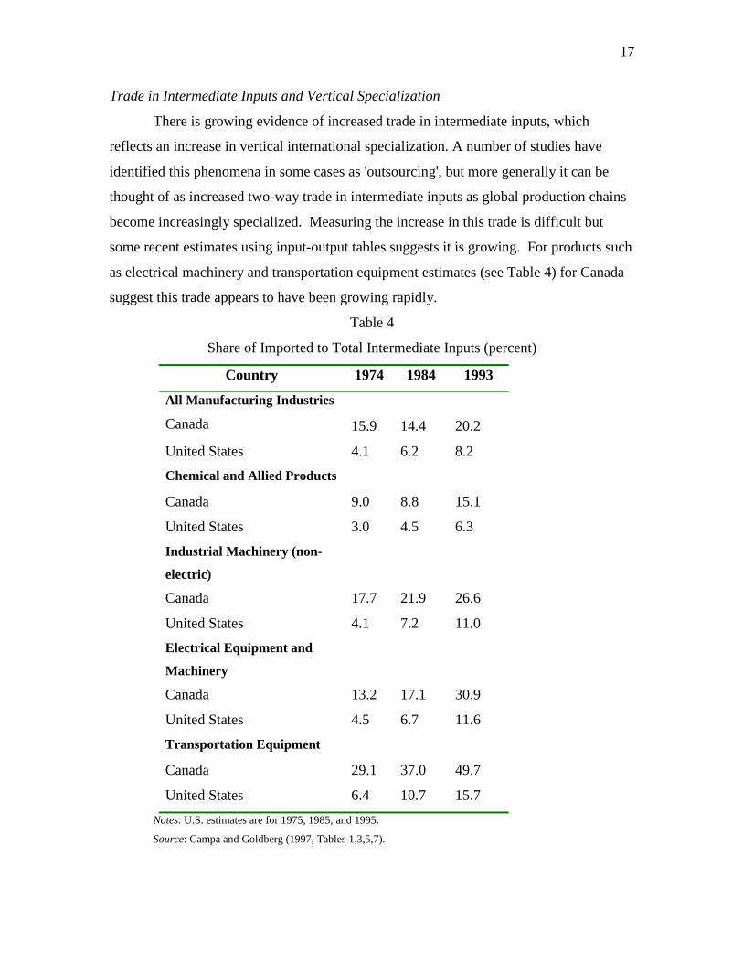
Trade in Intermediate Inputs and Vertical Specialization

There is growing evidence of increased trade in intermediate inputs, which

reflects an increase in vertical international specialization. A number of studies have

identified this phenomena in some cases as 'outsourcing', but more generally it can be

thought of as increased two-way trade in intermediate inputs as global production chains

become increasingly specialized. Measuring the increase in this trade is difficult but

some recent estimates using input-output tables suggests it is growing. For products such

as electrical machinery and transportation equipment estimates (see Table 4) for Canada

suggest this trade appears to have been growing rapidly.

Table 4

Share of Imported to Total Intermediate Inputs (percent)

Country 1974 1984 1993

All Manufacturing Industries

Canada 15.9 14.4 20.2

United States 4.1 6.2 8.2

Chemical and Allied Products

Canada 9.0 8.8 15.1

United States 3.0 4.5 6.3

Industrial Machinery (non-

electric)

Canada 17.7 21.9 26.6

United States 4.1 7.2 11.0

Electrical Equipment and

Machinery

Canada 13.2 17.1 30.9

United States 4.5 6.7 11.6

Transportation Equipment

Canada 29.1 37.0 49.7

United States 6.4 10.7 15.7Notes: U.S. estimates are for 1975, 1985, and 1995.

Source: Campa and Goldberg (1997, Tables 1,3,5,7).

18

There appears to evidence of increases in specialization within Canadian trade

patterns looked at from an intra-industry perspective and some weak evidence of

increased specialization at the inter-industry level. In general it is supportive of

Ricardian theories which appeal to specialization as a response to increased openness.

5. An Empirical model of Productivity Growth and Openness.

We now examine the empirical relationship between trade and productivity for

Canadian manufacturing. To recall, there was evidence of the levels gap closing at the

aggregate manufacturing level through the 80's; but since that time the gap appears to

have widened. The data we use compares the 1980-88 period to the 88-95 period.6 In a

number of ways this particular comparison may be unfortunate. As is well known the

Canadian economy was hit with a number of 'shocks' in the early 90's which may have

exacerbated the economic situation, including a slowdown in productivity growth. These

include tight monetary policy, a rapidly appreciating exchange rate, a political crisis, and

a fiscal crisis which necessitated sharp reductions in spending. The net effect was a

dramatic reduction in growth rates and as significant output gap according to

conventional macroeconomic calculations. See Fortin(1996) for a discussion. In

manufacturing the situation was not much better. According to BLS data there was a

5.75 percentage point gap in favor of the U.S. over the 1888-1995 period, between U.S.

and Canadian manufacturing output growth. However even during the 1980's the

situation was little different with US manufacturing output growth (cumulative) from

1980 to 1988 7 percentage points over the Canadian growth over the same period.

As noted in our previous discussion there are reasons to suspect a connection

between productivity growth and openness. We estimate an empirical openness and

growth equation for Canadian manufacturing for the period 1980-1995. We concentrate

on the two periods 1980-88 and 1988-1995 with the 88 break corresponding to the last

year prior to the CUSFTA. This also allows us to use some recent Industry Canada

estimates of productivity growth. The dependent variable is the annual growth in TFP

6 This data was kindly provided to us by Industry Canada and is the outcome of a large study which is also

being presented at this conference. See the paper by Wolong Gu and Mun Ho.

19

over the period express as a percentage. The openness variable can be measured in a

variety of ways but we chose to use OPEN measured by the ratio of exports to shipments.

The RATIO variable is the ratio of the Canadian to US TFP levels at the beginning of the

period which reflects the productivity gap by industry. Other variables are incorporated

including human capital (measured by the ratio of workers with university education to

total workers) (HUMAN) and various indexes of demand growth (DEMAND) thought to

be important from the Ricardian perspective.

itit5it4it3it21it DEMANDaHUMANaRATIOaOPENaaGTFP ε+++++=

This was estimated as a panel across the two periods with 17 manufacturing industries,

with some regressions including fixed effects for industries and a dummy for the post 88

period (time dummy) labeled FTA.. Results are reported in Table 5 for the models

without industry fixed effects and Table 6 with industry fixed effects. The model without

industry fixed effects has very little explanatory power. Adding Industry Fixed effects

improves the R-square. Some comments on the results worth noting.

1. The levels RATIO variable and openness variable are invariably insignificant

although of the correct sign when entered separately. However when entered

interactively so that increased openness is more valuable to countries with a higher

productivity gap, the coefficients become significant and of the correct sign. Thus

contrary to the general pessimism there appear to be evidence in favor of the

conditional convergence effect for Canadian manufacturing industries.

2. The FTA time dummy appears with a negative coefficient in the non-fixed effects

model. With industry fixed effects it is generally positive and marginally significant.

Model 4 allows for a slope dummy on the Open/Ratio variable and while of the

correct sign is not significant.

3. The Human capital variable generally is not significant which is somewhat surprising

given that is has shown up in a number of aggregate convergence and openness

studies.

4. The Demand growth variable is not significant without or without industry fixed

effects. Two demand models were tried-model 6 with growth in the value of exports

as the proxy for demand, and model 7 with U.S. output growth(real) proxying

demand growth in the same industry

20

Table 5

Productivity Dynamics

CAN_GTFP Model 1 Model 3

RATIO

OPEN

OPEN/RATIO 0.5037 0.5177

0.4940 0.490

FTA*OPEN/RATIO

HUMAN

DEMAND 3.67

2.9646

Time/Post FTA -0.1791

0.22415

-0.2450

0.2287

R-squared 0.03815 0.0797

* Significant, 90%

** Significant, 95%

21

Table 6

Productivity Dynamics-Industry Fixed Effects

CAN_GTFP Model 1 Model 2 Model 3 Model 4

RATIO -2.406 -1.149

1.316* 1.515

OPEN 6.504

4.285

OPEN/RATIO 7.041 6.088

2.484** 2.615** 2

FTA*OPEN/RATIO 1.032

0.9348

HUMAN

1

Time/Post FTA 0.112 0.624 0.739 0.133 0.838 0.019 1.132 0.015

R-squared 0.509 0.571 0.601 0.629

* Significant, 90%

** Significant, 95%

22

Table 6, continued.

CAN_GTFP Model 6 Model 7

RATIO(CAN/US)

OPEN

OPEN/RATIO 7.185 6.957

2.423** 2.5619**

FTA*OPEN/RATIO

HUMAN

DEMAND1 5.774

4.178

DEMAND2 0.03513

0.1002

Time 0.953 0.010 0.832 0.330

R-squared 0.644 0.604

On average the combined coefficient on the gap and openness ratio seems to be in

the range of 0.7 to 0.9. Given the increasing and substantial openness of the Canadian

economy this suggests the substantial gap in productivity levels, which the Industry

Canada study suggests stands at about 88 percent based on adjusted TFP comparisons.

One can translate that into about a 0.4 percent convergence effect per year for an

industry with an export to shipments ratio of 40 percent and the average productivity gap.

On the issue of demand effects there is no evidence that productivity growth was

concentrated in sectors with strong demand growth potential. We conclude (weakly) that

at least on that score there seems to a case that Canadian manufacturing missed the boat

in terms of concentrating its productivity efforts in those sectors where it could have had

23

greater impact. We are cautious however in this interpretation for two reasons. First,

there were a few sectors with spectacularly negative productivity growth in the 88-95

period including Printing. Lumber, and Stone, clay and glass products. It is possible the

FTA, and possibly commodity price developments were responsible for the unusual

productivity performance in these sectors. To the extent they constitute outliers they may

seriously be biasing the results. One could of course go on extensive specification

searches for other productivity drivers besides trade. Perhaps this conference will

provide us some useful suggestions as where to look.

5. Explaining the Pattern of Export Growth

We now ask the reverse question to that posed in the last section. Is the pattern of

trade which emerged over the period consistent with an improved aggregate productivity

performance, or in fact was it counterproductive? Note that this is related to another well

trodden issue --the testing of Ricardian trade models in which productivity explicitly

appears as a determinant of relative costs. Choudri and Schembri(1998) have recently

carried such an exercise using a more modern version of the theory. The purpose here

thought is slightly different. We are not interested in testing a structural model of trade.

Rather what is at issue here is the investment (and policy) decisions which within the

manufacturing sector which led to the observed pattern of specialization in Canada and

resulting export growth. To do this we estimate a simple model of real export growth

(value of exports deflated by a general selling price index). In line with a variety of

theories we expect the pattern of export growth to depend positively on productivity

growth, relative price increases, and a number of other potential variables. Under the

HOV model in particuular would like to control for factor intensity differences across

sectors to pick up Rybczinksi effects but we will ignore these due to data problems. A

failure to find growth positively associated with the cross sectional variation in TFP,

particularly in the both FTA period, would be be a smoking gun indicative of a flawed

pattern of comparative advantage. On the other hand if export growth is associated with

TFP growth this particular class of explanations for the 'gap' may be suspect.

In the Ricardian framework there should be a similar set of forces at work,

although ideally we would like to correct for other factors in addition to productivity

24

which would have led certain export sectors to expand relative to others. Ideally one

would like to control for the import competitiveness of the US industry. To do that we

will use US productivity growth.

It is useful to begin with a couple of scatter plots for the two-digit data of output

growth versus TFP growth and Relative Product Price changes. See figures 1 and 2 for

the post FTA years. There is a positive but fairly weak correlation between TFP and

output growth. With respect to relative prices however the expected positive association

associated from a small open economy supply side model does not appear at first cut to

be very evident. Other interpretations of this are obviously possible.

We begin first with the disaggregated 3-digit matched trade and industry data.

Three models of export growth on TFP growth are estimated. Model 1 include industry

effect, Model 2 does not have a time dummy for the FTA, and Model 3 has no industry

fixed effects. In all cases the TFP growth variable is insignificant and in the case of

Model 3 is actually negative. This suggests there is at first past little evidence of export

specialization in those sectors where productivity growth was high.

Table 7

Export Growth and TFP: 104 Industries

D-Export Growth Model 1 Model 2 Model 3

D-TFP growth .700

0.5912

0.518

0.6039

-0.1822

0.4540

FTA dummy -0.227 0.2079

1.931

R-square .606 0.673 .0142** Adjusted R-square.

The second model estimated is on the 2-digit data. In this case we control for two

additional factors. First, relative price changes across industries, and second,

productivity growth in the United States. Under the Ricardian model one would expect

that strong U.S. productivity growth would reduce exports in Canada. The estimated

model is a panel on the 80-88 and 88-95 periods using the same data as in the previous

section. Export growth is the dependent variable denoted by D-X regressed on the

25

change in Canadian TFP growth, D-TFPCAN, US-Productivity Growth, D-TFPUS, and

changes in relative price, D-PRICE.

Model 1 is the basis model with all effects included (there are industry fixed effects in

any of these results. Basically all the coefficients are insignficant, although the TFP

growth rates comes out with the correct sign. The Relative price term is virtually

insignficant in the models. The FTA dummy is postive in models 1 and 2 although its

effect is not large. When the FTA coefficient is interacted with Canadian productivity

growth this coefficent is significant. It remains signficant in fact with any of the other

variables included or excluded.

In general the conclusion is basically mildly negative. There is little evidence that

Canadian exports responded in a complementary way to the emerging pattern of

productivity growth in the 80-95 period. More puzzling is the fact that patterns of

relative export growth appear to be unrelated to relative price increases.

Table 8

Models of Export Growth

D-X Canada Model 1 Model 2 Model 3

D-TFP CAN .01408

.01238

0.0141

0.01194

D-TFP US -0.00103

0.0089

FTA*D-TFPCAN .0288**

.0135

D-PRICE 0.0012

0.0069

0.001261 0.0025

.0058

FTA DUMMY 0.0403

0.01435

0.0403

0.0140

R-Square .21208 0.1209

Conclusion to follow:

26

Bibliography

Abramovitz, M. (1986). "Catching Up, Forging Ahead and Falling Behind," Journal of EconomicHistory, 46:385–406

Ben-David, D. (1993). "Equalizing Exchange: Trade Liberalization and Income Convergence,"Quarterly Journal of Economics, 108(3):653–79.

Bernard, A.B and C.I Jones (1996). "Comparing Apples to Oranges: Productivity Convergenceand Measurement Across Industries and Countries," American Economic Review,December.

Bernard, A.S. and J.B. Jensen (1999). Exporting and Productivity, Working Paper No. 7135,National Bureau of Economic Research, Cambridge (Mass.).

Bernstein, J.I. (1994). International R&D Spillovers Between Industries in Canada and theUnited States, Working Paper No. 3, Industry Canada, Microeconomic Policy AnalysisBranch, September..

Choudri, E. H.and L. Schembri (1998) "Productivity Performance and InternationalCompetitiveness: A New Test of an Old Theory" mimeo, Economics, CarletonUniversity, Ottawa, Canada.

Easterly, W., M. Kremer, L. Pritchett and L. Summers (1993). "Good Policy or Good Luck?Country Growth Performance and Temporary Shocks," Journal of Monetary Economics,32:459–83.

Edwards, S. (1998), "Openness, productivity and growth: what do we really know?" EconomicJournal, pages 383-98.

Fortin, P. (1996). "The Great Canadian Slump," Canadian Journal of Economics, XXIX:761–87,November.

Fuentes-Goddoy, Paul Hansson and Lars Lundberg (1996) "International specialization andstructura change in Swedish Manufacturing, 1969-1992. Weltwirtschaftliches Archiv,132, No..3, 523-543.

Grady, P. and K. Macmillan (1998). "Why is Interprovincial Trade Down and International TradeUp," Canadian Business Economics, 6(4):26–35.

Grossman, G. and E. Helpman,, (1991a), Innovation and Growth in the Global Economy, MITPress.

Harris, R.G. (1998). "Long Term Productivity Issues," in T.J. Courchene and T.A. Wilson (eds.),Fiscal Targets and Economic Growth, John Deutsch Institute, Queen’s University,Kingston, p. 67–90.

Sachs, J.D and A. Warner (1995). "Economic Reform and the Process of Global Integration,"Brookings Papers on Economic Activity, p. 1–118.

27

Treffler, D. (1999). Canada's Lagging Productivity, Working Paper ECWP–125, EconomicGrowth and Policy Program , Canadian Institute for Advanced Research, Toronto.

28

Figure 1

Figure 2

Relationship Between Output Growth and Productivity Growth During 1988-1995

-2.5

-2

-1.5

-1

-0.5

0

0.5

1

1.5

2

-8 -6 -4 -2 0 2 4 6 8 10

Output Growth

Tota

l Fac

tor P

rodu

ctiv

ity G

row

thOutput Growth versus Relative Price Changes during

1988- 1995. (In Percentage)

-2.0000

-1.0000

0.0000

1.0000

2.0000

3.0000

4.0000

-2.25 -1.75 -1.25 -0.75 -0.25 0.25 0.75 1.25 1.75

Output Growth

Rel

ativ

e Pr

ice

Cha

nges