Productivity of Nations: A Stochastic Frontier Approach to TFP Decomposition

8/12/2019 Productivity of Nations: A Stochastic Frontier Approach to TFP Decomposition

http://slidepdf.com/reader/full/productivity-of-nations-a-stochastic-frontier-approach-to-tfp-decomposition 1/19

Hindawi Publishing CorporationEconomics Research InternationalVolume 2012, Article ID 584869, 19 pagesdoi:10.1155/2012/584869

Research ArticleProductivity of Nations: A Stochastic Frontier Approach toTFP Decomposition

Jorge Oliveira Pires1 and Fernando Garcia 2

1 Escola de Economia de S˜ ao Paulo, Fundac ao Getulio Vargas, Rua Itapeva, 474-11 S˜ ao Paulo, SP, Brazil 2 Confederac ¸˜ ao Nacional de Servic os, Rua Professor Tamandar e Toledo, 69-3 S˜ ao Paulo, SP, Brazil

Correspondence should be addressed to Jorge Oliveira Pires, [email protected]

Received 31 August 2011; Accepted 26 October 2011

Academic Editor: Magda E. Kandil

Copyright © 2012 J. O. Pires and F. Garcia. This is an open access article distributed under the Creative Commons AttributionLicense, which permits unrestricted use, distribution, and reproduction in any medium, provided the original work is properly cited.

This paper tackles the problem of aggregate TFP measurement using stochastic frontier analysis. We estimate a world productionfrontier for a sample of 75 countries over a long period. The “Bauer-Kumbhakar” decomposition of TFP is applied to asmaller sample in order to evaluate the eff ects of changes in efficiency (technical and allocative), scale eff ects, and technicalchange. Estimated technical efficiency scores are compared to productivity indexes off ered by nonfrontier studies. We concludethat diff erences in productivity are responsible for virtually all the diff erences of growth performance between developed anddeveloping nations and that a large part of this is due to allocative efficiency.

1. Introduction

This paper uses an alternative way of measuring total factorproductivity based on stochastic frontier analysis (SFA). Thegreat advantage of SFA is the possibility that it off ers of de-composing productivity change into parts that have straight-forward economic interpretation.

Previous studies have attempted to evaluate the efficiency and productivity growth of nations in the context of the so-called technical inefficiency literature, most of which usingdata envelopment analysis (DEA) techniques for a sample of OECD countries (e.g., Fare et al. [1]). Deliktas and Balcilar

[2, 3] have used SFA but in the context of a somewhat res-tricted time period of analysis (1991–2000) which permits amore comprehensive sample of countries (130-country fron-tier). However, they do not analyze or provide results aboutefficiency levels or rates of change of efficiency (or any othercomponent of TFP change) for the great majority of suchcountries, focusing their analysis only on 25 transition coun-tries. They do not study the role of allocative efficiency either.

The main contribution of our paper is to show that asuitable decomposition of TFP can be applied to a fairly largesample of heterogeneous countries for an extensive periodof time in order to evaluate not just the roles of technicalprogress and technical efficiency change, but also scale and

allocative efficiency change as determinants of long-termgrowth. We are not aware at this time of any other SFA study that has produced quantitative results showing that allocativeefficiency plays an important role in the economic growth of nations.

The stochastic frontier model used in this article assumesthe existence of technical inefficiency which evolves followinga particular behavior. This allows one to split productivity changes into (i) the change in technical efficiency, whichmeasures the movement of an economy towards (or away from) the production frontier, and (ii) technical progress,

which measures shifts of the frontier over time.When applied to a flexible technology (e.g., translog),

this technique further allows one to evaluate the presenceof scale efficiency. The Bauer-Kumbhakar decomposition(Bauer [4], Kumbhakar [5]) may then be applied, allowingthe additional measurement of changes in allocative effi-ciency. Our results show that this last component, togetherwith technical change, explains a large portion of the diff er-ences in economic growth between developed and develop-ing countries.

In the next section, we present the hypotheses behindthe stochastic frontier estimation and TFP decomposition.Section 3 presents the estimates of the world stochastic



2 Economics Research International

production frontier and discusses the technical efficiency scores obtained comparing them to productivity indexes sug-gested by Islam [6] and Hall and Jones[7]. Technical progressand returns to scale estimates are also discussed. In Section 4,we use the estimates of the previous section in order todecompose TFP change from 1965 up to 2000. The role

of technical progress and allocative effi

ciency change ineconomic growth of both developed and developing nationsis highlighted in Section 5. At last, in Section 6, we discussthe contribution of these results for the recent debate aboutthe sources of economic growth and the nature and role of TFP components.

2. SFA and TFP Decomposition

The approach adopted in this paper is that developed inthe literature on technical efficiency and productivity, morespecifically in the “statistical” and “parametric” branches of this literature, which is known as Stochastic Frontier Analysis

(SFA). The focus of SFA is to obtain an estimator for oneof the components of TFP, the degree of technical efficiency.Technical efficiency is estimated in addition to technicalchange which in its turn is captured (as usual) by a timetrend and interactions of the regressors with time. The modelused here is essentially that developed (independently) by Aigner et al. [8] and by Meeusen and van den Broeck [9].Their formulation was extended by Pitt and Lee [10] andSchmidt and Sickles [11] for the panel data case. Since thesetwo last mentioned studies, a number of enhancements havebeen suggested, such as that of Battese and Coelli [12], inwhich the technical inefficiency is modeled so as to be timevariant. A thorough compilation of this literature is found inKumbhakar and Lovell [13].

The general stochastic production frontier model is de-scribed by the equations below, where y is the vector for thequantities produced by the various countries, x is the vec-tor for production factors used, and β is the vector for theparameters defining the production technology.

y = f

t , x , β

· exp(v ) · exp(−u), u ≥ 0. (1)

The v and u terms (vectors) represent diff erent errorcomponents. The first one refers to the random part of theerror, while the second is a downward deviation from theproduction frontier (which can be inferred by the nega-tive sign and the restriction u ≥ 0). Thus, f (t , x , β) ·

exp(v ) represents the stochastic frontier of production and v has a symmetrical distribution to capture the random ef-fects of measuring errors and exogenous shocks that causethe position of the deterministic nucleus of the frontier, f (t , x , β), to vary from country to country. The level of tech-nical efficiency (TE), that is, the ratio of observed outputto potential output (given by the frontier) is captured by the component exp(−u) (note that TEit = y it / exp(x it β) =

exp(x it β − uit ) / exp(x it β) = exp(−uit ) and, therefore, 0 < TE< 1). For each country i and each time period t , we have

y it = f

t , x it , β

· exp(v it ) · exp(−uit );

i = 1, . . . , N , t = 1, . . . , T.(2)

Once it is assumed that v ∼ iid N (0, σ 2); u ∼

NT(µ, σ 2u ), that is, u has a normal-truncated distribution(with a nonnull average µ) the two error components areindependent of each other and x is supposed exogenous, themodel can be estimated by maximum-likelihood (ML) tech-niques and the restriction of a half-normal distribution (µ =

0) can be tested. Given these conditions, the traditional asy-mptotic properties of the ML estimators hold. In addition,we take the technical inefficiency component as time-variant,as suggested by Battese and Coelli [12]:

uit = exp

−η(t − T )

· ui, uit ≥ 0, i = 1, . . . , N , t ∈ τ (i).(3)

Other parameterizations of u are possible but we willnot pursue them here (see, e.g., Kumbhakar [14], Corn-well et al. [15], Lee and Schmidt [16]).

In expression (3), τ (i) represents the T i periods of time for which we have available observations for the i-nthcountry, among the available T periods in the panel (i.e.,

τ (i) may contain all periods in the panel or only a subsetof periods). The sign of η dictates the behavior of technicalinefficiency over time. When η is not significantly diff er-ent from zero, technical inefficiency does not vary in time(persistent inefficiency). This specification of the behavioralpattern of inefficiency is somewhat inflexible, as the model’sarchitects themselves admit. According to the formulation,technical inefficiency must; grow at decreasing rates (η > 0)or decrease at increasing rates (η < 0). Moreover, the estimat-ed value for η is the same for all countries in the sample,which means that the pattern of inefficiency rise or reductionis the same for all countries. Despite these limitations, webelieve the model can still bring very interesting insights into

the patterns of economic growth of nations.Assuming a translog technology with two production

factors, namely, capital (K ) and labor (L), the model can beexpressed in the following way:

ln y it = β0 + βt · t + βK ln K it + βL ln Lit + 0.5 · βtt · t 2

+ 0.5 · βKK (lnKit )2 + 0.5 · βLL(ln Lit )

2

+ 0.5 · βKL (ln K it ) · (ln Lit ) + βKt [(ln K it ) · t ]

+ βLt [(ln Lit ) · t ] + v it − uit .(4)

The output elasticities with respect to K and L can beobtained from (4), working out the derivatives. Due to theuse of a translog technology, these elasticities are country andtime specific. The technical progress measure is also specificfor each country and period of time and can be obtained by partial diff erentiation of the deterministic part of (4) withrespect to time.

Bauer [4] and Kumbhakar [5] suggested a quite inge-nious, yet simple, type of productivity decomposition whichgoes beyond the division of productivity changes into acatchup eff ect and a technical innovation eff ect. Such frame-work also accounts for scale eff ects and inefficient allocationof productive factors. To perform this decomposition, we



Economics Research International 3

must first estimate the model depicted by (3) and (4). Then,it is possible to “compose” the rate of total factor productivity change from the results. In the expressions that follow, dotsover variables indicate time derivatives, g TFP denotes the rateof TFP growth, sK and sL are the shares of capital and labor inaggregate income, and εK and εL are output elasticities with

respect to the factors of production.The components of productivity change can be identifiedfrom algebraic manipulations from the deterministic part of the production frontier depicted in (2) combined with theusual expression for the productivity change Divisia index:

g TFP =

˙ y

y − sK

K

K − sL

L

L. (5)

From the deterministic part of (2), we have

˙ y

y =

∂lnf

t , K , L, β

∂t + εK

K

K + εL

L

L −

∂u

∂t . (6)

In the expressions that follow, RTS denotes returns toscale with RTS = εK + εL, g K is the growth rate of capital( K/ K ) and g L is the growth rate of labor (L/L); λK = εK / RTSand λL = εL / RTS are defined as normalized shares of capitaland labor in income. Combining (5) and (6), we have

g TFP = TP − u + (RTS − 1) ·

λK · g K + λL · g L

+

( λK − sK ) · g K + ( λL − sL) · g L

.(7)

That is, total factor productivity growth can be split intofour elements:

(i) technical progress, measured by TP = ∂ ln f (t , K , L,

B) /∂t ;(ii) change in technical efficiency, denoted by −u;

(iii) change in the scale of production, given by (RTS−1)·

[ λK · g K + λL · g L];

(iv) change in allocative efficiency, measured by [( λK −

sK ) · g K + ( λL − sL) · g L].

We can now study the impact of each of the componentsof TFP. If the technology is immutable, it does not contributeto productivity gains. The same happens with technicalinefficiency. If it does not vary in time, it also does not haveany impact on the rate of change of productivity.

The contribution of economies of scale depends both on

technology as well as on factor accumulation. The presenceof constant returns to scale (RTS = 1) cancels out the thirdcomponent on the right of (7). In the case of increasingreturns to scale (RTS > 1) and an increase in the amountof productive factors, we have a higher rate of productivity growth. If the amounts of production factors diminish, thenwe would have a reduction in the rate of productivity change.An inverse analogous reasoning can be made for decreasingreturns and reduction (increase) in the amount of productivefactors.

Since λK + λL = 1, the distances ( λK − sK ) and ( λL − sL)are symmetric and have opposite signs. Therefore, a factorreallocation that, say, increases the intensity of labor and

reduces that of capital will necessarily bring a change inallocative efficiency. Only when there are no inefficiencies orscale eff ects is the measure of productivity change identicalto technical progress.

3. Estimation of the World StochasticFrontier (1950–2000)

The model estimation was conducted using statistics soft-ware STATA, which includes among its preprogrammedmodels that of Battese and Coelli [12]. The database for thisstudy consists of a nonbalanced panel for aggregated outputand production factors (K and L) of a sample of countriesthat includes both wealthy as well as poor nations. Thesedata were basically obtained from Penn World Tables (PWT),version 6.1, for years 1950 to 2000. Data for factor shareswere obtained from the System of National Accounts 1968(SNA68, United Nations [17]) and from the Annual National Accounts of OECD (OECD [18]). Since the constructionof a database that proved useful for conducting aggregateproductivity analysis using SFA techniques seems to be animportant contribution of this study, we choose not to justbriefly describe the data and sample here, but to do it moreextensively in Appendix A.

A number of alternative specifications were tested, im-posing diff erent restrictions on the parameters of the translogtechnology. Likelihood ratios tests allow us to check if suchrestrictions are valid or not. These statistics are presented inAppendix B. As a general result of these tests, we can say thatthe statistics favor the (complete) translog functional form.

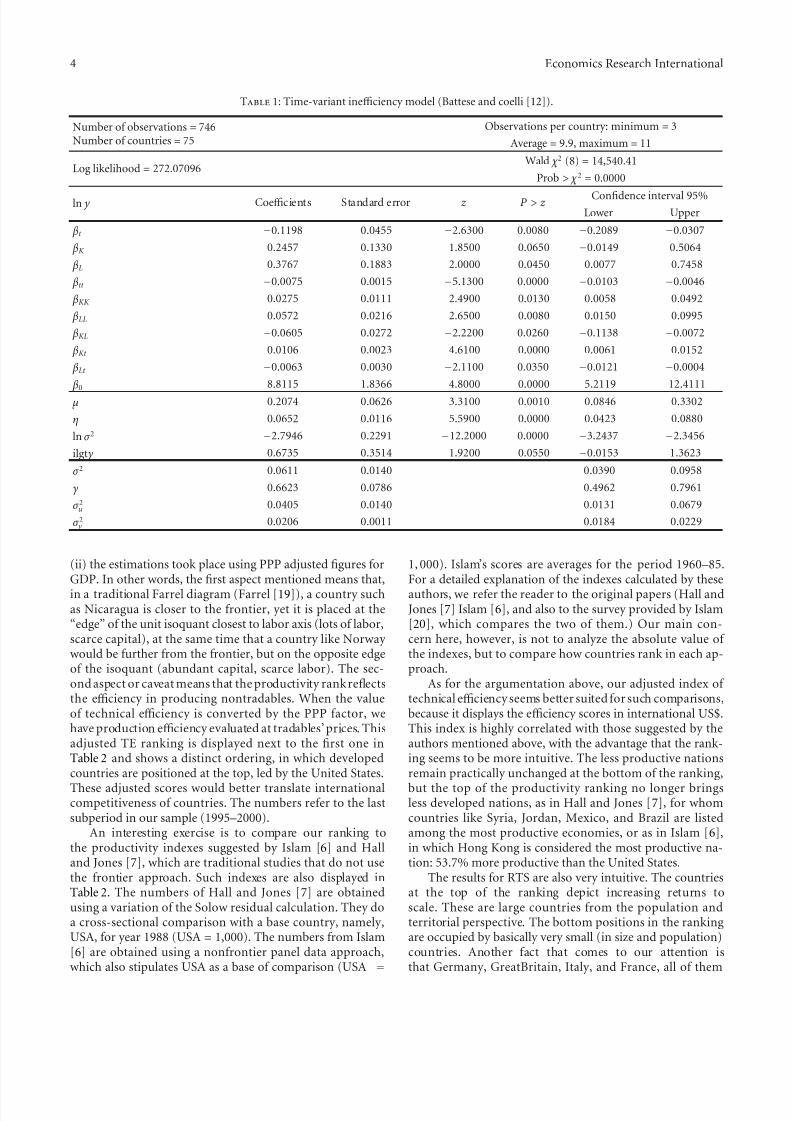
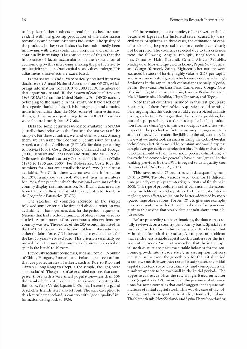
Results for the translog specification are presented inTable 1. All parameters are significant at 5%, except for thecapital elasticity of output, which is significant at 6.5%. Themean inefficiency µ is significantly diff erent from zero at1%, showing that the normal truncated distribution is anappropriate assumption (if it were not significant, we wouldfall back to the case of a half-normal distribution). Theestimated value of η is positive, which means that technicalefficiency grows at decreasing rates (catchup).

βKL is negative, revealing the possibility of substitutionbetween the production factors. The βt and βtt coefficientsindicate that the neutral part of technical progress has nega-tive eff ects on production and in order to achieve (positive)technical progress, it is necessary that the nonneutral partof technical progress off sets these eff ects. The signs of βKt

and βLt indicate, respectively, that the nonneutral part of technical progress goes hand in hand with capital accumu-lation (positive sign of βKt ), and inversely with labor supply (negative sign of βLt ), that is, technical progress is laborsavingand is more intense in countries where capital is abundant.

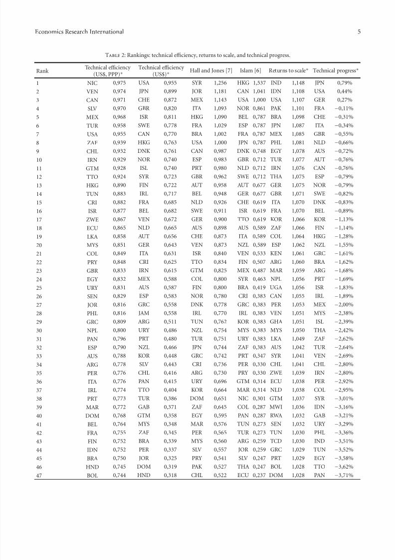
Inspection of the results for returns to scale, techni-cal change, and technical efficiency reveals that these areeconomically meaningful. Table 2 shows country ranks forRTS, TE, and TP. The technical efficiency ranking must beviewed with caution. Although the presence of countries likeNicaragua, Venezuela, and El Salvador in the first positionsdoes indeed seem odd, two aspects must be kept in mind:(i) these results are “conditional” on the capital-labor ratio;




Table 1: Time-variant inefficiency model (Battese and coelli [12]).

Number of observations = 746Number of countries = 75

Observations per country: minimum = 3

Average = 9.9, maximum = 11

Log likelihood = 272.07096 Wald χ 2 (8) = 14,540.41

Prob > χ 2 = 0.0000

ln y Coefficients Standard error z P > z Confidence interval 95%Lower Upper

βt −0.1198 0.0455 −2.6300 0.0080 −0.2089 −0.0307

βK 0.2457 0.1330 1.8500 0.0650 −0.0149 0.5064

βL 0.3767 0.1883 2.0000 0.0450 0.0077 0.7458

βtt −0.0075 0.0015 −5.1300 0.0000 −0.0103 −0.0046

βKK 0.0275 0.0111 2.4900 0.0130 0.0058 0.0492

βLL 0.0572 0.0216 2.6500 0.0080 0.0150 0.0995

βKL −0.0605 0.0272 −2.2200 0.0260 −0.1138 −0.0072

βKt 0.0106 0.0023 4.6100 0.0000 0.0061 0.0152

βLt −0.0063 0.0030 −2.1100 0.0350 −0.0121 −0.0004

β0 8.8115 1.8366 4.8000 0.0000 5.2119 12.4111

µ 0.2074 0.0626 3.3100 0.0010 0.0846 0.3302

η 0.0652 0.0116 5.5900 0.0000 0.0423 0.0880

ln σ 2 −2.7946 0.2291 −12.2000 0.0000 −3.2437 −2.3456

ilgtγ 0.6735 0.3514 1.9200 0.0550 −0.0153 1.3623

σ 2 0.0611 0.0140 0.0390 0.0958

γ 0.6623 0.0786 0.4962 0.7961

σ 2u 0.0405 0.0140 0.0131 0.0679

σ 2v 0.0206 0.0011 0.0184 0.0229

(ii) the estimations took place using PPP adjusted figures forGDP. In other words, the first aspect mentioned means that,in a traditional Farrel diagram (Farrel [19]), a country suchas Nicaragua is closer to the frontier, yet it is placed at the“edge” of the unit isoquant closest to labor axis (lots of labor,scarce capital), at the same time that a country like Norway would be further from the frontier, but on the opposite edgeof the isoquant (abundant capital, scarce labor). The sec-ond aspect or caveat means that the productivity rank reflectsthe efficiency in producing nontradables. When the valueof technical efficiency is converted by the PPP factor, wehave production efficiency evaluated at tradables’ prices. Thisadjusted TE ranking is displayed next to the first one inTable 2 and shows a distinct ordering, in which developedcountries are positioned at the top, led by the United States.

These adjusted scores would better translate internationalcompetitiveness of countries. The numbers refer to the lastsubperiod in our sample (1995–2000).

An interesting exercise is to compare our ranking tothe productivity indexes suggested by Islam [6] and Halland Jones [7], which are traditional studies that do not usethe frontier approach. Such indexes are also displayed inTable 2. The numbers of Hall and Jones [7] are obtainedusing a variation of the Solow residual calculation. They doa cross-sectional comparison with a base country, namely,USA, for year 1988 (USA = 1,000). The numbers from Islam[6] are obtained using a nonfrontier panel data approach,which also stipulates USA as a base of comparison (USA =

1, 000). Islam’s scores are averages for the period 1960–85.For a detailed explanation of the indexes calculated by theseauthors, we refer the reader to the original papers (Hall andJones [7] Islam [6], and also to the survey provided by Islam[20], which compares the two of them.) Our main con-cern here, however, is not to analyze the absolute value of the indexes, but to compare how countries rank in each ap-proach.

As for the argumentation above, our adjusted index of technical efficiency seems better suited for such comparisons,because it displays the efficiency scores in international US$.This index is highly correlated with those suggested by theauthors mentioned above, with the advantage that the rank-ing seems to be more intuitive. The less productive nationsremain practically unchanged at the bottom of the ranking,

but the top of the productivity ranking no longer bringsless developed nations, as in Hall and Jones [7], for whomcountries like Syria, Jordan, Mexico, and Brazil are listedamong the most productive economies, or as in Islam [6],in which Hong Kong is considered the most productive na-tion: 53.7% more productive than the United States.

The results for RTS are also very intuitive. The countriesat the top of the ranking depict increasing returns toscale. These are large countries from the population andterritorial perspective. The bottom positions in the rankingare occupied by basically very small (in size and population)countries. Another fact that comes to our attention isthat Germany, GreatBritain, Italy, and France, all of them




Table 2: Rankings: technical efficiency, returns to scale, and technical progress.

Rank Technical efficiency

(US$, PPP)∗

Technical efficiency (US$)∗

Hall and Jones [7] Islam [6] Returns to scale∗ Technical progress∗

1 NIC 0,975 USA 0,955 SYR 1,256 HKG 1,537 IND 1,148 JPN 0,79%

2 VEN 0,974 JPN 0,899 JOR 1,181 CAN 1,041 IDN 1,108 USA 0,44%

3 CAN 0,971 CHE 0,872 MEX 1,143 USA 1,000 USA 1,107 GER 0,27%

4 SLV 0,970 GBR 0,820 ITA 1,093 NOR 0,861 PAK 1,101 FRA −0,11%

5 MEX 0,968 ISR 0,811 HKG 1,090 BEL 0,787 BRA 1,098 CHE −0,31%

6 TUR 0,958 SWE 0,778 FRA 1,029 ESP 0,787 JPN 1,087 ITA −0,34%

7 USA 0,955 CAN 0,770 BRA 1,002 FRA 0,787 MEX 1,085 GBR −0,55%

8 ZAF 0,939 HKG 0,763 USA 1,000 JPN 0,787 PHL 1,081 NLD −0,66%

9 CHL 0,932 DNK 0,761 CAN 0,987 DNK 0,748 EGY 1,078 AUS −0,72%

10 IRN 0,929 NOR 0,740 ESP 0,983 GBR 0,712 TUR 1,077 AUT −0,76%

11 GTM 0,928 ISL 0,740 PRT 0,980 NLD 0,712 IRN 1,076 CAN −0,76%

12 TTO 0,924 SYR 0,723 GBR 0,962 SWE 0,712 THA 1,075 ESP −0,79%

13 HKG 0,890 FIN 0,722 AUT 0,958 AUT 0,677 GER 1,075 NOR −0,79%

14 TUN 0,883 IRL 0,717 BEL 0,948 GER 0,677 GBR 1,071 SWE −

0,82%15 CRI 0,882 FRA 0,685 NLD 0,926 CHE 0,619 ITA 1,070 DNK −0,83%

16 ISR 0,877 BEL 0,682 SWE 0,911 ISR 0,619 FRA 1,070 BEL −0,89%

17 ZWE 0,867 VEN 0,672 GER 0,900 TTO 0,619 KOR 1,066 KOR −1,13%

18 ECU 0,865 NLD 0,665 AUS 0,898 AUS 0,589 ZAF 1,066 FIN −1,14%

19 LKA 0,858 AUT 0,656 CHE 0,873 ITA 0,589 COL 1,064 HKG −1,28%

20 MYS 0,851 GER 0,643 VEN 0,873 NZL 0,589 ESP 1,062 NZL −1,55%

21 COL 0,849 ITA 0,631 ISR 0,840 VEN 0,533 KEN 1,061 GRC −1,61%

22 PRY 0,848 CRI 0,625 TTO 0,834 FIN 0,507 ARG 1,060 BRA −1,62%

23 GBR 0,833 IRN 0,615 GTM 0,825 MEX 0,487 MAR 1,059 ARG −1,68%

24 EGY 0,832 MEX 0,588 COL 0,800 SYR 0,463 NPL 1,056 PRT −1,69%

25 URY 0,831 AUS 0,587 FIN 0,800 BRA 0,419 UGA 1,056 ISR −1,83%

26 SEN 0,829 ESP 0,583 NOR 0,780 CRI 0,383 CAN 1,055 IRL −1,89%

27 JOR 0,816 GRC 0,558 DNK 0,778 GRC 0,383 PER 1,053 MEX −2,00%

28 PHL 0,816 JAM 0,558 IRL 0,770 IRL 0,383 VEN 1,051 MYS −2,38%

29 GRC 0,809 ARG 0,511 TUN 0,762 KOR 0,383 GHA 1,051 ISL −2,39%

30 NPL 0,800 URY 0,486 NZL 0,754 MYS 0,383 MYS 1,050 THA −2,42%

31 PAN 0,796 PRT 0,480 TUR 0,751 URY 0,383 LKA 1,049 ZAF −2,62%

32 ESP 0,790 NZL 0,466 JPN 0,744 ZAF 0,383 AUS 1,042 TUR −2,64%

33 AUS 0,788 KOR 0,448 GRC 0,742 PRT 0,347 SYR 1,041 VEN −2,69%

34 ARG 0,778 SLV 0,443 CRI 0,736 PER 0,330 CHL 1,041 CHL −2,80%

35 PER 0,776 CHL 0,416 ARG 0,730 PRY 0,330 ZWE 1,039 IRN −2,80%

36 ITA 0,776 PAN 0,415 URY 0,696 GTM 0,314 ECU 1,038 PER −2,92%

37 IRL 0,774 TTO 0,404 KOR 0,664 MAR 0,314 NLD 1,038 COL −

2,95%38 PRT 0,773 TUR 0,386 DOM 0,651 NIC 0,301 GTM 1,037 SYR −3,01%

39 MAR 0,772 GAB 0,371 ZAF 0,645 COL 0,287 MWI 1,036 IDN −3,16%

40 DOM 0,768 GTM 0,358 EGY 0,595 PAN 0,287 RWA 1,032 GAB −3,21%

41 BEL 0,764 MYS 0,348 MAR 0,576 TUN 0,273 SEN 1,032 URY −3,29%

42 FRA 0,755 ZAF 0,345 PER 0,565 TUR 0,273 TUN 1,030 PHL −3,36%

43 FIN 0,752 BRA 0,339 MYS 0,560 ARG 0,259 TCD 1,030 IND −3,51%

44 IDN 0,752 PER 0,337 SLV 0,557 JOR 0,259 GRC 1,029 TUN −3,52%

45 BRA 0,750 JOR 0,325 PRY 0,541 SLV 0,247 PRT 1,029 EGY −3,58%

46 HND 0,745 DOM 0,319 PAK 0,527 THA 0,247 BOL 1,028 TTO −3,62%

47 BOL 0,744 HND 0,318 CHL 0,522 ECU 0,237 DOM 1,028 PAN −3,71%




Table 2: Continued.

Rank Technical efficiency

(US$, PPP)∗

Technical efficiency (US$)∗

Hall and Jones [7] Islam [6] Returns to scale∗ Technical progress∗

48 SWE 0,742 EGY 0,286 THA 0,513 CHL 0,225 BEL 1,028 MAR −3,71%

49 NLD 0,738 COL 0,281 ECU 0,504 DOM 0,214 SWE 1,023 CRI −3,73%

50 CHE 0,738 BOL 0,252 LKA 0,481 PAK 0,194 HND 1,022 JAM −3,80%

51 RWA 0,737 TUN 0,252 BOL 0,469 PHL 0,186 AUT 1,021 ECU −3,95%

52 PAK 0,734 ECU 0,250 PAN 0,463 BOL 0,169 SLV 1,020 DOM −4,02%

53 TCD 0,722 PRY 0,242 HND 0,449 JAM 0,169 HKG 1,018 PRY −4,10%

54 GAB 0,720 NIC 0,237 NIC 0,443 EGY 0,153 CHE 1,017 JOR −4,25%

55 DNK 0,713 SEN 0,226 JAM 0,410 LKA 0,153 NIC 1,017 SLV −4,29%

56 LSO 0,708 LSO 0,210 PHL 0,389 HND 0,126 PRY 1,016 GTM −4,39%

57 NZL 0,703 MAR 0,209 IND 0,344 NPL 0,120 ISR 1,015 LKA −4,48%

58 AUT 0,700 PHL 0,203 SEN 0,316 SEN 0,110 JOR 1,014 PAK −4,53%

60 KOR 0,692 LKA 0,188 ZWE 0,275 UGA 0,104 DNK 1,010 BOL −4,58%

61 JAM 0,678 ZWE 0,185 NPL 0,244 ZWE 0,104 FIN 1,010 HND −4,90%

62 GER 0,677 THA 0,176 RWA 0,242 IND 0,071 CRI 1,006 ZWE −4,90%

63 NOR 0,659 KEN 0,161 KEN 0,237 KEN 0,071 NOR 1,006 LSO −5,19%64 ISL 0,654 RWA 0,159 GHA 0,215 RWA 0,065 IRL 1,004 NIC −5,24%

65 IND 0,640 UGA 0,158 UGA 0,162 MWI 0,058 URY 1,004 KEN −5,32%

66 GHA 0,637 PAK 0,146 TCD 0,151 GHA 0,053 NZL 1,003 GHA −5,49%

67 UGA 0,635 TCD 0,138 MWI 0,130 TCD 0,042 PAN 1,000 SEN −5,50%

68 SYR 0,632 IDN 0,136 JAM 0,998 NPL −5,94%

69 JPN 0,621 GHA 0,119 LSO 0,994 MWI −6,10%

70 KEN 0,611 NPL 0,118 TTO 0,981 UGA −6,19%

71 THA 0,595 IND 0,109 GAB 0,975 RWA −6,43%

72 MWI 0,502 MWI 0,102 ISL 0,939 TCD −6,56%

Source: Islam [20], Table 11.3 page 485–488], and own estimations. Hall and Jones indexes depicted here are equal to exp (log A), in Table 9 of Hall and Jones(1996) [7].

(∗) Annual average rates 1996–2000. Three countries were left out due to lack of information for this subperiod.

European nations of very homogeneous characteristics, areplaced next each other in the ranking.

The results for technical progress seem at first sight ratherodd, with almost all of them being negative. (Although mostof the numbers for Technical progress (TP) in Table 2 arenegative, they refer only to the last subperiod of our sample,that is, 1996–2000. TP presented a pattern in which it startspositive and then shows a decaying trend along the sub-periods in the sample.) Nonetheless, the ordering seems tomatch our intuition regarding the technological performance

of nations. At the top positions are Japan, United States, Ger-many, and France. Among the countries at the bottom arethe African nations, wellknown for their lack of technologicalknowledge.

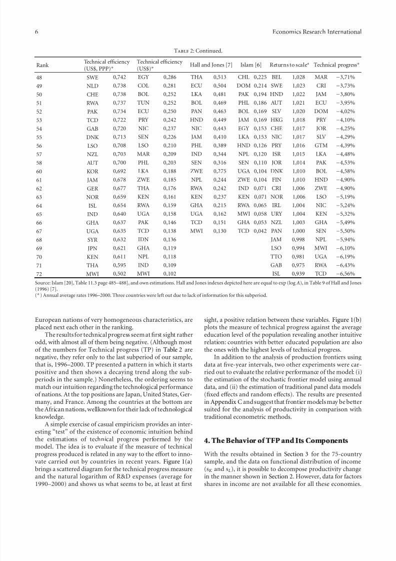
A simple exercise of casual empiricism provides an inter-esting “test” of the existence of economic intuition behindthe estimations of technical progress performed by themodel. The idea is to evaluate if the measure of technicalprogress produced is related in any way to the eff ort to inno-vate carried out by countries in recent years. Figure 1(a)brings a scattered diagram for the technical progress measureand the natural logarithm of R&D expenses (average for1990–2000) and shows us what seems to be, at least at first

sight, a positive relation between these variables. Figure 1(b)plots the measure of technical progress against the averageeducation level of the population revealing another intuitiverelation: countries with better educated population are alsothe ones with the highest levels of technical progress.

In addition to the analysis of production frontiers usingdata at five-year intervals, two other experiments were car-ried out to evaluate the relative performance of the model: (i)the estimation of the stochastic frontier model using annualdata, and (ii) the estimation of traditional panel data models

(fixed eff ects and random eff ects). The results are presentedin Appendix C and suggest that frontier models may be bettersuited for the analysis of productivity in comparison withtraditional econometric methods.

4. The Behavior of TFP and Its Components

With the results obtained in Section 3 for the 75-country sample, and the data on functional distribution of income(sK and sL), it is possible to decompose productivity changein the manner shown in Section 2. However, data for factorsshares in income are not available for all these economies.




R&D expenditures (Millions of US$)—average 1990–2000

T e c h n i c a l p r o g r e s s ( p . a

. % )

VEN

USA

THA

SWE

PRT

PHL

MYS

MEX

KOR

JPN

ITA

ISL

IND

GER

DNK

CHL

CHE

BRA

AUS

ARG

1 0

2 0 3 0 4 0 5 0

1 0 0

2 0 0 3 0 0 4 0 0

5 0 0

1

. 0 0 0

2

. 0 0 0

3

. 0 0 0

4

. 0 0 0

5

. 0 0 0

1 0 . 0 0 0

2 0 . 0 0 0

3 0 . 0 0 0

4 0 . 0 0 0

5 0 . 0 0 0

1 0 0 . 0 0 0

2 0 0 . 0 0 0

3 0 0 . 0 0 0

−0.05

−0.04

−0.03

−0.02

−0.01

0

0.01

(a)

T e c h n i c a l p r o

g r e s s ( p . a . % )

Average years of schooling of population over 25 years

14121086420

ZWE

VEN

USA

UGA

THA

SWE

SEN

PRT

PHL

PAK

MYS

MEX

LSO

KOR

JPN

ITA

ISL

IND

GER FRA

ESP DNK

COL CHL

CHE

BRA

AUS

ARG

−0.1

−0.1

−0.0

−0.0

0

0

(b)

Figure 1: R&D Expenditures, human capital and technicalprogress. Sources: own estimations and World Development Indica-tors (World Bank) for R&D and Schooling. Technical progress ratesare averages for 1996–2000.

We managed to collect data for only 36 of the 75 countries inthe sample, and just from 1970 up to 2000. The full decom-position of TFP is then restricted to this group and period.Table 3 brings the results.

Examination of average productivity change numbersalong the 30 years in question shows some interesting results.All top positions are occupied by OECD countries. Among

them, Japan’s performance stands out, with an averageannualproductivity growth rate of 2.42%. The countries that follow are Austria (1.77%), France (1.75%), Norway (1.53%), Swit-zerland (1.51%), and USA (1.49%). In the middle block, wefind some Latin American countries, such as Jamaica, Brazil,Peru, Venezuela, and Bolivia, all of them with relatively low

TFP growth rates. Brazil showed an average rise in producti-vity of 0.39% per year. Among the other Latin Americancountries in the sample, we see that Mexico, Costa Rica, and,surprisingly, Chile had reductions in productivity. Greeceand Turkey are the only OECD members with negativeproductivity growth during this time.

Countries for which technical progress (TP) showedthe greatest impact on productivity growth were Japan, theUnited States, France, Switzerland, Italy, United Kingdom,The Netherlands, and Australia, in this order. Contributionsof TP for this group of countries ranged from 0.56 to 0.30percent per year, on average. As we can see, they are all de-veloped nationsthat invest substantial amounts in R&D.

Among the 19 countries that presented positive contri-butions of technical progress, 18 are OECD members (seeTable 3). As mentioned before, for many countries, the lastsubperiod (1996–2000) reveals negative technical progress(as shown in Table 2). Notwithstanding that, in Table 3, wedepict positive average annual contributions of TP to growthfor 19 countries (of the total 36). These numbers are averagescalculated for the longer period 1970–2000.

Brazil is the only member of OECD that managed tohave technical progress contributing for higher productivity,mainly in the 1965 to 1985 period. This trend matches thatof three other Latin American countries that underwent amarked import substitution process, namely, Mexico, Peru,and Venezuela. The fall in the pace of technical progress of these countries coincides with the debt crisis and economicliberalization, periods during which the industrializationprocess slows down its pace.

An important aspect pertains to the interpretation of technical regress (negative technical progress) that appears inthe results of this study (other authors also report this kindof result using frontier techniques—Rao and Coelli [21] isan example). First, it should be pointed out that a frontierwas not estimated for each country and, therefore, it is nota matter of saying that this or that country had “inward”shifts to their frontiers. The interpretation is quite difficultin light of the way that technical progress was achieved, by including a time trend in the model (and interactions of

time with capital and labor). According to Arrow [22], thisprocedure, which is rather common in the literature, is mostof all a confession of ignorance. As discussed in Section 3, theunderlying idea here is that countries closer to the frontier(and on the forefront of technical progress) are responsiblefor the actual shift in the world production frontier.

One way of interpreting technical regress in less devel-oped nations is that it may be the result of circumstances ordecisions that end up halting the production of some high-technology products and encouraging the manufacturing of low-technology products. Since GDP is the aggregation of value added in a number of industries, this sliding perfor-mance could be the result of production shifting from some




Table 3: Sources of economic growth 1970–2000: average annual % change.

Country 1Economicgrowth

2Capitalaccumulation

2Laborexpansion

Productivity change Random3

shocksTFP

Technicalprogress

Technicalefficiency

Scaleeff ects

Allocativeefficiency

AUS 4.16 1.17 1.06 0.93 0.30 0.46 0.06 0.12 1.00

AUT 3.74 1.70 0.30 1.77 0.25 0.69 0.01 0.81 −

0.03BEL 3.29 1.60 0.31 1.40 0.23 0.52 0.03 0.61 −0.02

BOL 2.73 1.68 1.00 0.05 −0.55 0.57 0.00 0.02 0.00

BRA 5.59 4.51 1.13 0.39 0.01 0.55 0.41 −0.58 −0.44

CAN 4.14 1.87 1.10 0.98 0.26 0.06 0.12 0.54 0.19

CHE 2.03 1.31 0.52 1.51 0.40 0.59 −0.01 0.53 −1.30

CHL 4.98 3.88 0.87 −0.41 −0.30 0.13 0.11 −0.35 0.64

COL 4.93 3.73 1.05 −0.20 −0.30 0.31 0.20 −0.41 0.34

CRI 4.89 4.01 1.63 −0.32 −0.47 0.24 −0.12 0.03 −0.43

DNK 2.61 0.89 0.35 1.39 0.27 0.65 −0.01 0.47 −0.02

ESP 3.97 2.79 0.54 1.30 0.23 0.45 0.17 0.44 −0.66

FIN 3.65 1.76 0.37 1.45 0.18 0.55 −0.02 0.74 0.07

FRA 3.43 1.79 0.47 1.75 0.41 0.54 0.15 0.64 −0.57

GBR 2.73 0.99 0.27 1.33 0.32 0.35 0.10 0.55 0.13

GRC 3.67 4.37 0.30 −0.46 0.05 0.41 0.04 −0.95 −0.55

IRL 6.03 2.18 0.61 0.97 −0.05 0.49 −0.04 0.56 2.27

ISL 4.13 1.22 0.93 0.97 −0.09 0.82 −0.21 0.46 1.01

ITA 3.53 2.14 0.29 1.24 0.35 0.49 0.15 0.25 −0.14

JAM 1.80 2.06 0.86 0.41 −0.43 0.75 −0.08 0.18 −1.54

JOR 6.23 5.95 2.17 −0.83 −0.63 0.39 −0.14 −0.45 −1.06

JPN 5.26 3.54 0.58 2.42 0.56 0.92 0.34 0.57 −1.28

KEN 5.17 3.22 1.48 0.07 −0.79 0.95 0.16 −0.24 0.39

KOR 9.31 6.93 0.88 0.62 −0.03 0.71 0.40 −0.46 0.87

MEX 5.00 4.57 1.27 −

0.18 −

0.07 0.06 0.34 −

0.51 −

0.66NLD 3.59 1.20 0.65 1.27 0.30 0.58 0.05 0.34 0.46

NOR 4.09 1.75 0.40 1.53 0.25 0.81 −0.03 0.50 0.41

NZL 2.39 0.47 0.77 0.76 0.15 0.68 −0.02 −0.05 0.39

PER 3.15 2.75 1.00 0.21 −0.20 0.49 0.10 −0.17 −0.81

PRT 4.71 3.09 0.39 1.20 −0.02 0.50 0.05 0.67 0.03

SWE 2.57 0.96 0.36 1.44 0.28 0.57 0.01 0.57 −0.20

THA 8.01 6.51 0.62 −0.73 −0.29 1.00 0.37 −1.79 1.60

TTO 3.62 2.65 0.83 −0.23 −0.41 0.15 −0.16 0.18 0.36

TUR 5.38 5.93 0.79 −1.33 −0.26 0.08 0.33 −1.48 −0.01

USA 3.97 1.70 0.84 1.49 0.52 0.09 0.28 0.59 −0.07

VEN 1.82 2.24 1.41 0.06 −0.10 0.05 0.08 0.04 −1.90

(1) Growth of GDP; (2) Growth rates adjusted by income shares; (3) Obtained as a residual.

highly productive sectors to others, where productivity islower. To test this hypothesis is beyond the scope of thispaper and would require an analysis disaggregated by sectorsof activity (an interesting example of a disaggregate study is Kim and Han [23], which analyses several South Koreanindustries using the Bauer-Kumbhakar decomposition).

All countries enjoyed rising technical efficiency as shownby the positive numbers in Table 3. That is a characteristicof the estimated model. The Battese and Coelli [ 12] modelimposes the restriction of a common η to all countries.

In the sample including all 75 countries, the estimatedvalue for this parameter was positive, which resulted in acatchup pattern for all countries: technical efficiency grows atdecreasing rates. The countries that had the largest catchupswere Thailand, Kenya, Japan, Iceland, Norway, Jamaica, andSouth Korea.

It is quite intuitive that Thailand, Japan, and South Koreashould appear at the top here, since they have made greateff ort to absorb technology and educate their people. Forthe other countries, however, this conclusion does not seem




to be so obvious. Nonetheless, Kenya, Iceland, and Jamaicaenjoyed very high rates of growth during some periods inthe sample, revealing a movement towards the frontier whosecause could only be understood following a deeper inves-tigation of the history of these economies (something beyondthe scope of this study). Among countries with low technical

effi

ciency improvements are the United States and Canadawhich is reasonable, since both these nations are already closeto the frontier. They are in fact pushing the frontier further.

It is plausible to suppose that countries with vast massesof population are those set to gain the most from scale eff ects.That is exactly the result obtained, with Brazil, South Korea,Thailand, Mexico, Japan, Turkey, and the USA showing largenumbers for this component. All of them but Japan and theUSA are usually referred to as “developing” nations and havesurely experienced leaping growth during some subperiodsof the sample, most of which based on factor accumulation.This accumulation also paved the way to productivity growthbased on scale. It is also rather intuitive that countries withsmall population have gained less, or even lost productivity,as witnessed by the results of Ireland, Jamaica, Costa Rica,Jordan, Trinidad and Tobago, and Iceland.

The estimated model produces scores that reflect thelevels of technical efficiency of these nations, but not levelsof allocative efficiency. The eff ects of allocative efficiency areonly evaluated in dynamic terms and reflect either an approx-imation or a departure of the value of the estimated sharesof income factors ( λK and λL) from their competitive values(i.e., factor remuneration from its marginal products). Asshown in Table 3, countries that had the largest allocativeefficiency gains were Austria, Finland, Portugal, France,Belgium, the United States, and Japan. At the other end arecountries that lost out with the dynamics of factor allocation.Most of the Latin American countries fall within this group,as well as South Korea (until 1985) and Thailand. Some of OECD’s poorest members are also among those countriesthat had poor performance in allocative efficiency terms,such as Greece and Turkey.

We see systematic gains with factor allocation in richereconomies and losses (or very modest gains) in poorer ones.It is interesting to point out that the diff erences betweenthese two groups of countries regarding changes in allocativeefficiency are even more marked in the first three five-yearperiods of the sample. It is well known that both Brazil andThailand decided on a strategy of “growth without adjust-ment” in response to the oil shock of 1973, with increasing

debt during this time. In Brazil the II National DevelopmentPlan was being implemented and government played animportant role in resource allocation in the economy and wasresponsible for large infrastructure investments. The impor-tance of government in resource allocation is also a charac-teristic of South Korea during the early years in the sample.

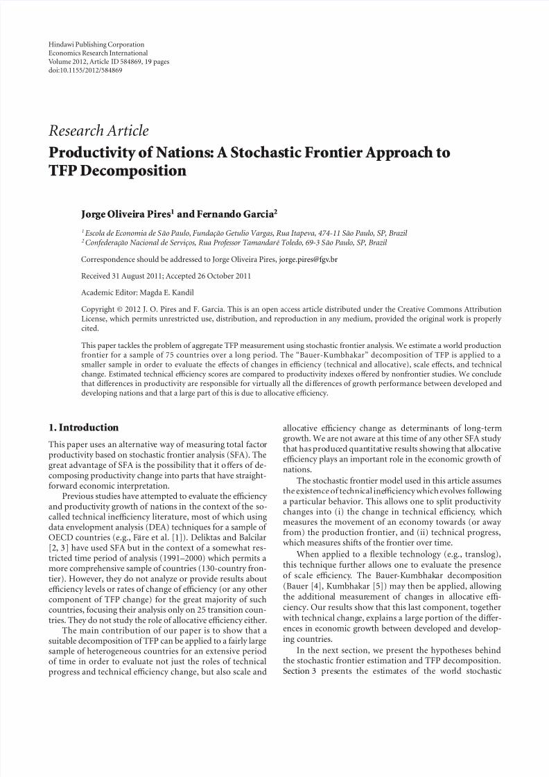
Figure 2 shows the evolution of total factor productivity change in six economies, calculated in two ways: (i) withallocative efficiency and (ii) without this component. Thefirst aspect to be highlighted is the distinct patterns of behav-ior displayed by developed and developing nations. France,the United States, and Japan present dynamic gains withresources allocation, and for them TFP computing allocative

efficiency remains above the measure that excludes thiscomponent. The opposite happens in Brazil for most of thesample period and in all of it for Mexico. South Korea, on theother hand, has a distinct pattern, in which the curves crosseach other, that is, allocative efficiency inverts its impact,becoming a driver for productivity gains in that country.

For Brazil, TFP computed without allocative effi

ciency is usually superior showing the eff ects of “ill allocation” of production factors. From the mid 1980s to the mid 1990s,this tendency reverses and begins to contribute to producti-vity growth, even if very little.After that period, the contribu-tion turns negative again, but not as large as in the first five- year periods under study. Mexico also reduces the negativeallocative eff ects as of the mid 1980s, but never enough tocontribute to a rise in productivity. For those two countries,the improvement in allocative efficiency roughly coincideswith market-oriented reforms. A significant relationship be-tween such phenomena remains to be tested though. On theother hand, Figure 2 also shows that rich nations such as Fra-nce, the United States, and Japan have persistent gains withallocative efficiency.

5. The Role of Technical Progress and Allocative Efficiency in Economic Growth

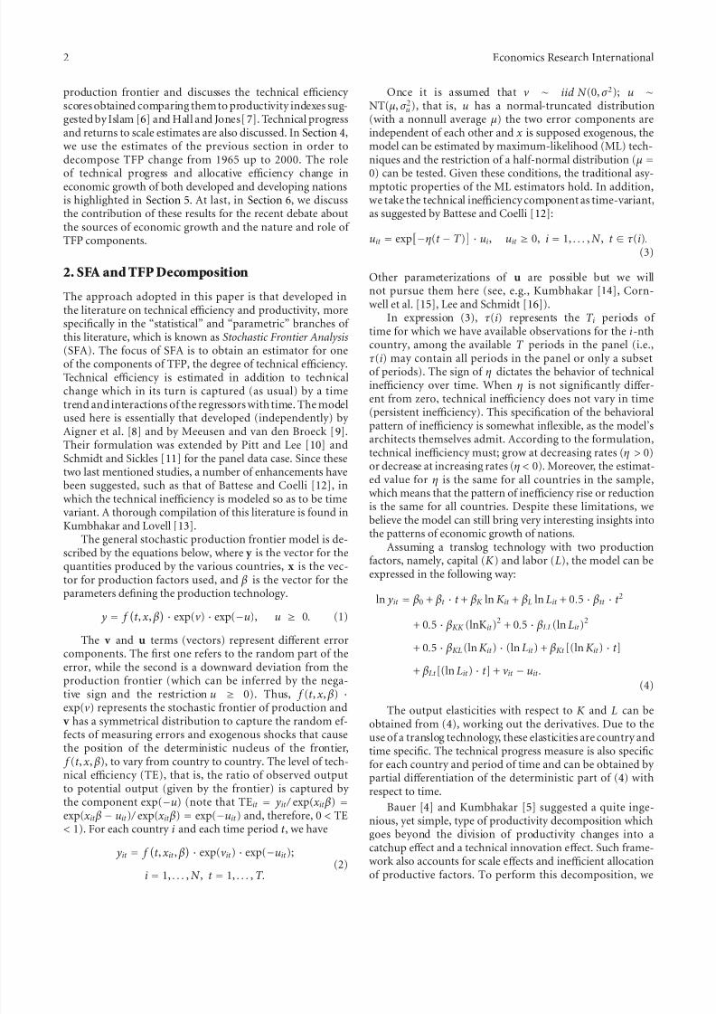
We will now take a closer look at the diff erences in eco-nomic growth patterns of developed and developing nations.Table 4 and Figure 3 bring results on the sources of growthfor those two groups of countries. The group of developednations consists of OECD member countries except Mexico,Greece, and Turkey, which are in the developing nationsgroup. This last group includes, in addition to the abovethree, all other countries in the sample (total of 36 countries).Table 4 displays annual averages for each five-year period andalso for the whole thirty-year period.

We see that developing nations grew more than devel-oped ones (18.2%). This happened because both capitalaccumulation and labor expansion were larger in developingcountries. However, the growth of GDP per worker wasgreater in developed countries, which can be attributed basi-cally to two factors: (i) the diff erence between the growthrates of capital and labor was greater in developed nations,thus providing higher growth of capital per worker; (ii) thechange in TFP in developed nations was considerably higherthan in developing ones (yet it should be said that in the sec-

ond group this change pushed down GDP’s growth). The dif-ferences between the two groups in regard to growth of cap-ital per worker are well below the diff erences in TFP growth.This suggests that productivity plays a role of great impor-tance in the development of nations, better yet, that it mightexplain a significant part of the diff erences in GDP per cap-ita growth between rich and poor countries.

If we take a look at the relative importance of the com-ponents of productivity, we see that developed nations havesome advantages, even if minor, in regard to technical effici-ency. On the other hand, we also see that this diff erence isin part off set by positive scale eff ects enjoyed by developingcountries. Judging by the magnitude of the diff erences




With allocative efficiency

Brazil

2000199519901985198019751970

Mexico

2000199519901985198019751970

Korea

2000199519901985198019751970

Japan

2000199519901985198019751970

France

2000199519901985198019751970

USA

2000199519901985198019751970

Without allocative efficiency

With allocative efficiency

Without allocative efficiency

−0.04

−0.02

0

0.02

0.04

0.06

0.08

0.04

0.06

0.08

0.1

0.12

0.14

0.16

0.18

0.04

0.06

0.08

0.1

0.12

0.14

−0.03

−0.02

−0.01

0

0

0.01

0.02

0.02

0.04

0.06

0.08

0.1

0.12

0

0.02

0.03

0.04

−0.1

−0.05

0

0.5

0.1

0.15

Figure 2: Total factor productivity change, with and without allocative efficiency.

between the groups of countries regarding the pace of technical progress and the evolution of allocative efficiency,we are able to conclude that these two components explainmost of the diff erences in productivity existing between thetwo groups.

While developed nations enjoyed technical progress of 7.2% in the 30 years analyzed here, developing countries infact suff ered a 9.8% drop in that component, a gap that addsup to 18.8%. We also notice that rich countries accumulated

sizable 12.5% in allocative efficiency improvement, at thesame time that in poor countries this variable fell 11%. Here,we have an accumulated diff erence of 26.4% in this com-ponent, which places this figure at the forefront in explainingthe diff erences in productivity among the two groups of countries, and consequently the diff erences in the rates of output growth.

Lower rates of growth of output per worker in develop-ing nations in comparison with developed ones lead to




Table 4: Sources of economic growth per group of countries and subperiods: % change.

Variable Group of

countries∗

Annual averages in the sub-periods Annualaverage

Accumulated1966–1970 1971–1975 1976–1980 1981–1985 1986–1990 1991–1995 1996–2000

GDP growth

Developed 5.33 3.92 3.44 2.30 3.62 2.04 3.57 4.04 228.22

Developing 5.29 5.14 5.64 1.93 3.38 4.12 2.90 4.74 301.10

Diff erence 0.03 −1.16 −2.08 0.37 0.23 −2.00 0.65 −0.67 −18.17

Capitalaccumulation

Developed 5.58 5.84 4.34 3.14 2.99 2.44 2.53 4.48 272.60

Developing 6.54 6.72 6.59 5.04 3.85 4.13 3.59 6.09 489.67

Diff erence −0.90 −0.83 −2.11 −1.81 −0.82 −1.63 −1.02 −1.52 −36.81

Laborexpansion

Developed 0.97 1.19 0.89 0.77 0.59 0.85 0.65 0.98 34.14

Developing 2.95 2.82 2.81 2.68 2.41 2.15 1.91 2.96 139.92

Diff erence −1.93 −1.59 −1.87 −1.86 −1.78 −1.27 −1.24 −1.92 −44.09

Change inGDP perworker

Developed 4.32 2.70 2.53 1.52 3.01 1.17 2.91 3.03 144.68

Developing 2.27 2.25 2.76 −0.73 0.95 1.92 0.98 1.73 67.18

Diff erence 2.00 0.43 −0.22 2.27 2.04 −0.74 1.91 1.28 46.36

Change incapital perworker

Developed 4.57 4.59 3.42 2.35 2.39 1.57 1.87 3.46 177.76

Developing 3.49 3.79 3.68 2.30 1.40 1.94 1.65 3.04 145.78

Diff erence 1.05 0.77 −0.25 0.05 0.98 −0.36 0.22 0.41 13.02

Change inTFP

Developed 1.32 1.56 1.34 1.04 0.97 0.68 0.59 1.25 45.14

Developing 0.07 −0.10 −0.23 −0.11 −0.16 −0.35 −0.37 −0.21 −6.11

Diff erence 1.25 1.66 1.58 1.15 1.14 1.03 0.97 1.46 54.58

Technicalprogress

Developed 0.54 0.44 0.33 0.21 0.09 −0.04 −0.17 0.23 7.22

Developing 0.04 −0.06 −0.16 −0.28 −0.41 −0.53 −0.66 −0.34 −9.76

Diff erence 0.50 0.50 0.49 0.49 0.50 0.49 0.49 0.58 18.82

Change intechnicalefficiency

Developed 0.56 0.53 0.49 0.46 0.43 0.40 0.38 0.54 17.63

Developing 0.43 0.40 0.37 0.35 0.33 0.31 0.29 0.41 13.13

Diff erence 0.13 0.13 0.12 0.11 0.10 0.10 0.09 0.13 3.98

Change in

scaleefficiency

Developed 0.05 0.06 0.06 0.06 0.07 0.07 0.07 0.07 2.25

Developing 0.01 0.07 0.10 0.10 0.13 0.14 0.14 0.12 3.53

Diff erence 0.04 0.00 −0.04 −0.04 −0.07 −0.07 −0.07 −0.04 −1.24

Change inallocativeefficiency

Developed 0.17 0.52 0.45 0.30 0.38 0.24 0.31 0.39 12.50

Developing −0.40 −0.50 −0.54 −0.28 −0.21 −0.26 −0.14 −0.39 −10.99

Diff erence 0.57 1.02 1.00 0.59 0.59 0.49 0.45 0.78 26.40∗

The values in this table were calculated by taking simple arithmetic averages over the countries comprising each group of the rates of change for eachsubperiod. The accumulated eff ects as well as the annual average numbers were computed by compounding (or discounting) rates. The relative factor pricesand relative marginal productivity of each period used in our calculations refers to the last year of the 5-year interval; for example, the values of sK , sL, λK ,and λL used to estimate the allocative efficiency changes between 1966 and 1970 refer to 1970.

divergence between the standards of living of the twogroups. In light of this, common aspects among countries

having similar growth patterns (and similar behavior forthe diff erence between the two measures of TFP mentionedbefore—with and without allocative efficiency) should besought and their motivation explored. The remarks madeat end of Section 4 are speculations on this topic and relatethese common aspects to policy.

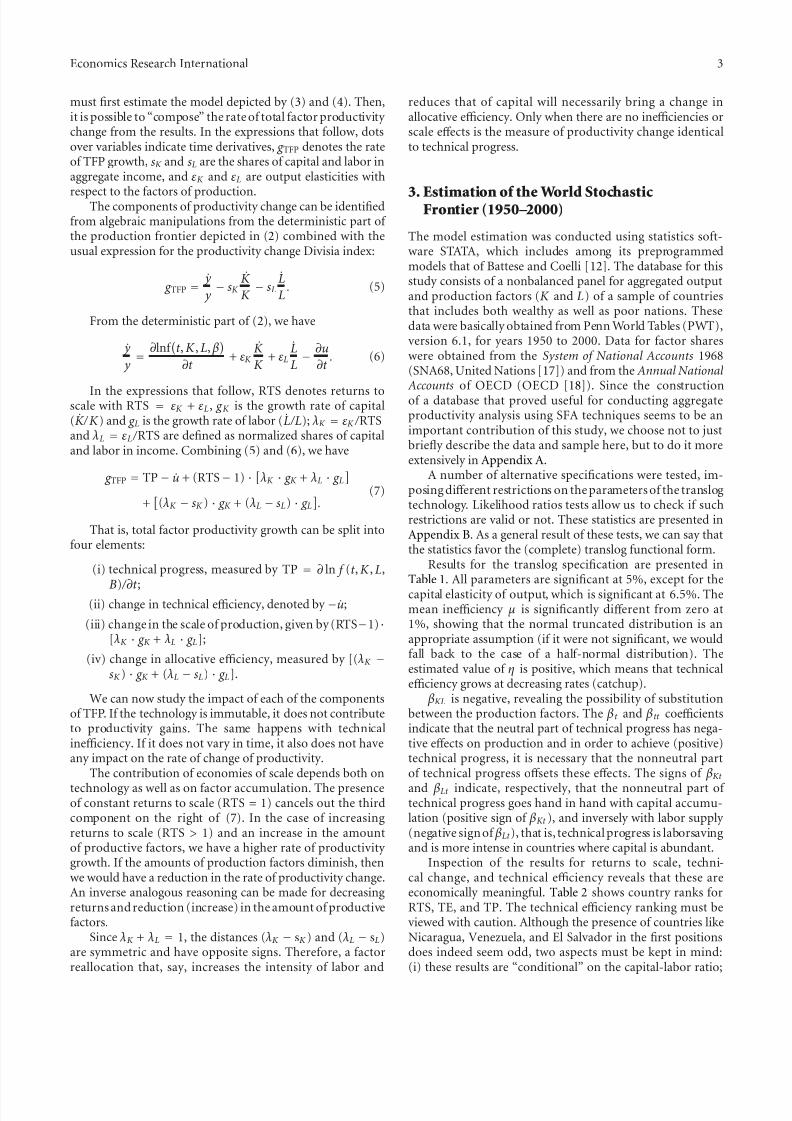
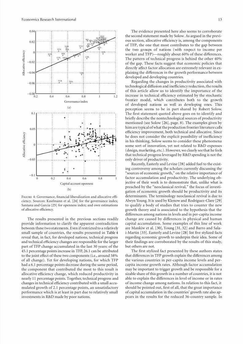
The allocative nature of policy eff ects is captured in arather informal way in Figure 4, where the measure of alloca-tive efficiency estimated here is plotted against two indi-cators (that, hopefully, do reflect policy). One is the Gover-nance Index developed by Kaufmann et al. [24] and the otheris the degree of capital account openness, according to themeasure suggested by Santana and Garcia [25]. As expected,

the economies with better governance in 1998 enjoyed lessdistortions and consequently greater allocative gains between

1995 and 2000 as depicted in Figure 4(a). Figure 4(b) plotsthe allocative efficiency measure against the openness index mentioned (for 33 of the 36 economies) from 1970 to 2000.Here, we have five-year changes in these two measures, andwe can see that reduction in barriers to capital flow seems tobe associated with improvements in allocative efficiency.

6. SFA and Recent Issues in theEconomic Growth Literature

Two excerpts from contemporary remarks made by RobertSolow reveal that much remains to be clarified regarding




Developing countries

2000199519901985198019751970

C o n t r i b u t i o n o f f a

c t o r a c c u m u l a t i o n

2000199519901985198019751970

C o n t r i b u

t i o n o f T F P

2000199519901985198019751970

T e c h n i c a l p r o g r e s s

2000199519901985198019751970

T e c h n i c a l e f fi c i e n c y

2000199519901985198019751970

S c a l e e f fi c i e n c y

2000199519901985198019751970

A l l o c a t i v e e f fi c i e n c y

−0.1

−0.05

0 0

0.05

0.1

0.15

0.2

0.25

−0.1

−0.05

0.05

0.1

0.15

0.2

0.25

−0.04

−0.02

0

0.02

0.04

0.06

0.08

−0.04

−0.02

0

0.02

0.04

0.06

0.08

−0.04

−0.02

0

0.02

0.04

0.06

0.08

−0.04

−0.02

0

0.02

0.04

0.06

0.08

Developed countries

Developing countries

Developed countries

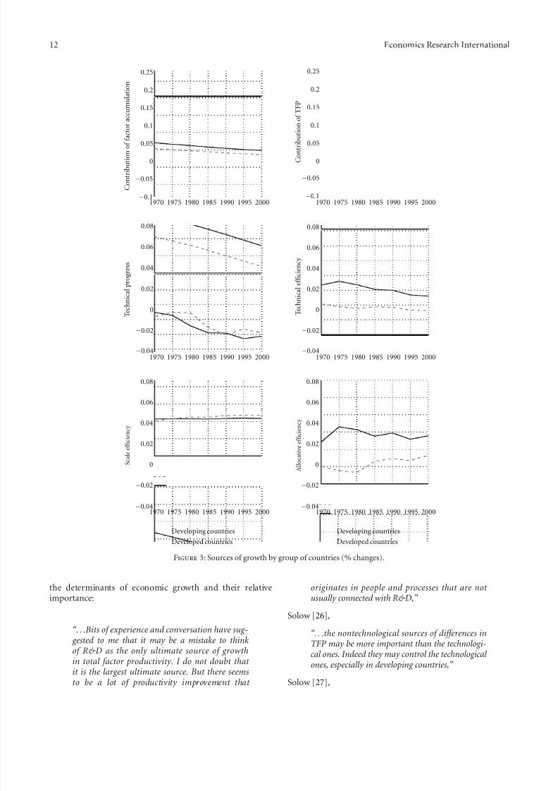
Figure 3: Sources of growth by group of countries (% changes).

the determinants of economic growth and their relativeimportance:

“ . . .Bits of experience and conversation have suggested to me that it may be a mistake to thinkof R&D as the only ultimate source of growthin total factor productivity. I do not doubt that it is the largest ultimate source. But there seemsto be a lot of productivity improvement that

originates in people and processes that are not usually connected with R&D,”

Solow [26] ,

“ . . .the nontechnological sources of di ff erences inTFP may be more important than the technologi-cal ones. Indeed they may control the technological ones, especially in developing countries,”

Solow [27],




0.2 0.4 0.6 0.8 1 1.2

Governance index

A l l o c a t i v e e f

fi c i e n c y

VEN

USA

TUR

TTO

THA

SWE

PRT

PER NZL

NOR NLD

MEX

KOR KEN

JPN

JOR

JAM ITA

ISLIRL

GRC

GBR

FRAFIN

ESP

DNK

CRI

COL CHL

CHE

CAN

BRA

BOL

BELAUT

AUS

−0.08

−0.06

−0.04

−0.02

0

0.02

0.04

(a)

0.2 0.4 0.6 0.8 1

0

0

Capital account openness

A l l o c a t i v e e

f fi c i e n c y

0.05

0.1

−0.1

−0.05

(b)

Figure 4: Governance, financial liberalization and allocative effi-ciency. Sources: Kaufmann et al. [24] for the governance index;Santana and Garcia [25] for openness index; and own estimationsof allocative efficiency.

The results presented in the previous sections readily provide information to clarify the apparent contradictionbetween these two statements. Even if restricted to a relatively small sample of countries, the results presented in Table 4reveal that, in fact, for developed nations, technical progress

and technical efficiency changes are responsible for the largerpart of TFP change accumulated in the last 30 years: of the45.1 percentage points increase in TFP, 26.1 can be attributedto the joint eff ect of these two components (i.e., around 58%of all change). Yet for developing nations, for which TFPhad a 6.1 percentage points decrease during the same period,the component that contributed the most to this result isallocative efficiency change, which reduced productivity innearly 11 percentage points. Together, technical progress andchanges in technical efficiency contributed with a small accu-mulated growth of 2.1 percentage points, an unsatisfactory performance which is at least in part due to relatively smallinvestments in R&D made by poor nations.

The evidence presented here also seems to corroboratethe second statement made by Solow. As argued in the previ-ous section, allocative efficiency is, among the componentsof TFP, the one that most contributes to the gap betweenthe two groups of nations (with respect to income perworker and TFP)—roughly about 60% of these diff erences.

The pattern of technical progress is behind the other 40%of the gap. These facts suggest that economic policies thatdirectly aff ect factor allocation are extremely relevant in ex-plaining the diff erences in the growth performance betweendeveloped and developing countries.

Regarding the changes in productivity associated withtechnological diff usion and inefficiency reduction, the resultsof this article allow us to identify the importance of theincrease in technical efficiency estimated by the stochasticfrontier model, which contributes both to the growthof developed nations as well as developing ones. Thisperception seems to be in part shared by Robert Solow.The first statement quoted above goes on to identify andbriefly describe the nontechnological sources of productivity mentioned (see Solow [26], page. 8). The examples given by him are typical of what the production frontier literature callsefficiency improvement, both technical and allocative. Sincehe does not consider the explicit possibility of inefficiency in his thinking, Solow seems to consider these phenomenasome sort of innovation, yet not related to R&D expenses(design, marketing, etc.). However, we clearly see that he feelsthat technical progress leveraged by R&D spending is not theonly driver of productivity.

Recently, Easterly and Levine [28] added fuel to the exist-ing controversy among the scholars currently discussing the“sources of economic growth,” on the relative importance of factor accumulation and productivity. The underlying ob- jective of their work is to demonstrate that, unlike what ispreached by the “neoclassical revival,” the focus of investi-gation of economic growth should be productivity and itsdeterminants. The terminology neoclassical revival is due toAlwyn Young. It is used by Klenow and Rodrıguez-Clare [29]to qualify a body of studies that tries to counter the new growth theory and is associated to the hypothesis that thediff erences among nations in levels and in per-capita incomechange are caused by diff erences in physical and humancapital accumulation. Some examples of this line of work are Mankiw et al. [30], Young [31, 32] and Barro and Sala-i-Martin [33]. Easterly and Levine [28] list five stylized factsregarding economic growth to underpin their idea. Some of

their findings are corroborated by the results of this study,but others are not.

The first stylized fact presented by these authors statesthat diff erences in TFP growth explain the diff erences amongthe various countries in per-capita income levels and per-capita income growth rates. Although factor accumulationmay be important to trigger growth and be responsible for asizable share of this growth in a number of countries, it is notable to explain the diff erences in level of income or in ratesof income change among nations. In relation to this fact, itshould be pointed out, first of all, that the great importanceof capital accumulation in the countries’ growth rate also ap-pears in the results for the reduced 36-country sample. In




fact, we find that 80% of the growth would be attributableto the accumulation of capital and labor, and only the20% remaining would come from productivity gains. Theresults vary when we calculate separately the average forthe group of 24 developed countries (factor accumulationis lower, close to 63% of the growth) and for the group

of 12 developing nations (contribution to productivity isnegative and, therefore, the factor accumulation is behind allthe economic growth).

If the reference is output per worker, the importance of capital accumulation remains high. With some additionalcalculations based on the numbers listed in Table 4, weconclude that on average 62.1% of the GDP growth is dueto capital accumulation. Klenow and Rodrıguez-Clare [29]reach a similar result for a sample of 98 countries: on average70% of economic growth is the result of physical and humancapital accumulation. The comparison is obviously limit-ed, because human capital is not considered in this study andbecause the samples are diff erent. Nonetheless, the reducedsample used in this article contains 24 of the 30 OECDmembers, while the sample used by Klenow and Rodrı-guez-Clare [29] contains all of them. Consequently, we canconclude that most of the nations that diff erentiate the twosamples are developing economies, which generally have ahigher share of capital in income. Thus, the inclusion of thesecountries would tend to raise the participation of factors inthe growth of GDP per worker (above 62.1%), bringing theresults of the two studies closer to each other.

Regarding income per capita, the diff erence between richand poor nations is the second stylized fact pointed out by Easterly and Levine [28]. According to them, this phenome-non is not very consistent with the analytical apparatus thatemphasizes factor accumulation with diminishing returnsand lack of economies of scale. It would be more appropriateto emphasize productivity growth based on technology andincreasing returns. Klenow [34] argues, however, that insti-tutional frameworks (such as tax structure, protectionism,lack of property rights,) may reduce the accumulation of physical and human capital. In line with the ideas suggestedby Easterly and Levine [28], the results of this article rejectan interpretation based on factor accumulation for this dis-crepancy.

The divergence between developed and developing na-tions was one of the results found using the empirical modelapplied in this study. Moreover, it is clear that the diff er-ences in the rates of productivity change are behind all the

diff erences in the rates of growth of GDP per worker (theaccumulation of factors contributed towards reducing suchdiff erences). Note that this result was obtained within thetraditional framework of an aggregated production functionwith diminishing returns. It was not necessary to incorporatein the analysis a new sector (a knowledge production sectorpresenting increasing returns).

The third stylized factor in the list of Easterly and Levine[28] suggests that the accumulation of factors is persistent,at the same time that economic growth is not. Consideringthat changes in the rate of growth depend both on changes infactor accumulation as well as on changes in productivity, thevalidity of this stylized fact impliesthat TFP cannot be persis-

2000199519901985198019751970

A v e r a g e o f r a n d o m e

r r o r c o m p o n e n t

Developed

Developing

−0.02

−0.015

−0.01

−0.005

0

0.005

0.01

0.015

0.02

Figure 5: Average random error component by group of countries,1970 to 2000.

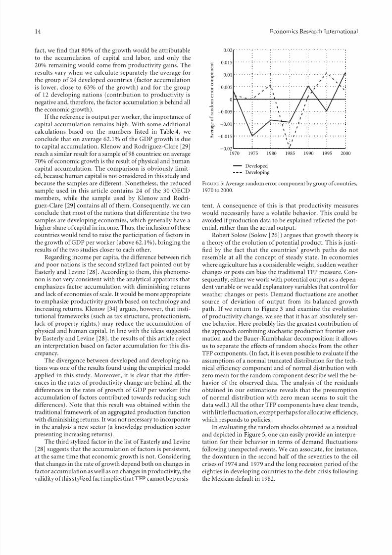
tent. A consequence of this is that productivity measureswould necessarily have a volatile behavior. This could beavoided if production data to be explained reflected the pot-ential, rather than the actual output.

Robert Solow (Solow [26]) argues that growth theory isa theory of the evolution of potential product. This is justi-fied by the fact that the countries’ growth paths do notresemble at all the concept of steady state. In economieswhere agriculture has a considerable weight, sudden weatherchanges or pests can bias the traditional TFP measure. Con-sequently, either we work with potential output as a depen-dent variable or we add explanatory variables that control forweather changes or pests. Demand fluctuations are anothersource of deviation of output from its balanced growthpath. If we return to Figure 3 and examine the evolutionof productivity change, we see that it has an absolutely ser-ene behavior. Here probably lies the greatest contribution of the approach combining stochastic production frontier esti-mation and the Bauer-Kumbhakar decomposition: it allowsus to separate the eff ects of random shocks from the otherTFP components. (In fact, it is even possible to evaluate if theassumptions of a normal truncated distribution for the tech-nical efficiency component and of normal distribution withzero mean for the random component describe well the be-havior of the observed data. The analysis of the residuals

obtained in our estimations reveals that the presumptionof normal distribution with zero mean seems to suit thedata well.) All the other TFP components have clear trends,with little fluctuation, except perhaps for allocative efficiency,which responds to policies.

In evaluating the random shocks obtained as a residualand depicted in Figure 5, one can easily provide an interpre-tation for their behavior in terms of demand fluctuationsfollowing unexpected events. We can associate, for instance,the downturn in the second half of the seventies to the oilcrises of 1974 and 1979 and the long recession period of theeighties in developing countries to the debt crisis followingthe Mexican default in 1982.




The fourth stylized fact points out that production fac-tors tend to flow towards the same direction and as a conse-quence economic activity is quite concentrated. This is validnot only among countries but also within them (regions,states, and cities). If there were no productivity diff erences,the trend would be exactly the opposite, that is, that of an

even distribution of factors among the various countries,because of the presence of decreasing returns. Diff erencesin policies could explain factor accumulation (regulation,tax structure, legal systems, public education, etc.). However,usually these policies have a nationwide scope and would notbe helpful in explaining concentration within the nations.Easterly and Levine [28] do not provide a single explanationfor this phenomenon and argue that such stylized fact isconsistent with existing explanations in terms of poverty traps, intragroup factors, or geographical externalities andis also consistent with explanations based on diff erences of productivity caused by technological diff erences.

The results of this article have shown that developingnations accumulate production factors at a much faster pacethan that of developed nations and for this reason also grow faster. The model used presents a measure of scale eff ects forthe sample countries that is intuitive but not fully consistentwith the notion of concentration of economic activity.Although the estimated measure of scale eff ects for develop-ing economies came up suggesting increasing returns to scale(for India, Indonesia, Brazil, and Mexico, to name a few), themagnitude of these eff ects is not up to the task of explainingthe fourth stylized fact identified by Easterly and Levine [28].

The fifth and last stylized fact states that policiesimplemented by nations have a relevant impact on long-term growth rates of these nations. The authors try to show that variables related to policy decisions of nationwidescope, such as education, degree of trade and financialliberalization, and size of the government, among otherfactors, are related to countries’ growth rates and to TFP. Thisis consistent with our results since changes in governmentpolicy have fundamental impacts on allocative efficiency.We believe to have shown the great importance of allocativeefficiency change in productivity change, and consequently in growth rate diff erences.

With a clear economic interpretation and the advantageof separating random shocks from the regular behavior of theeconomies, the stochastic frontier approach combined withflexible functional forms (for production frontiers) and theTFP decomposition described here seems to be a promising

way of looking at aggregate productivity, one up to the task of providing a broad range of explanations in the field of economic growth.

Appendices

A. Data and Sample

Below, we detail the definitions of each series used in theeconometric estimations. We also describe the proceduresused in selecting the countries and the time periods thatactually comprise the econometric estimations.

The output variable used is GDP measured at constantprices (1996 US$), with purchasing power parity (PPP)adjustment. It is obtained by taking the real GDP per capitachain series (RGDPPCH) from PWT 6.1 and multiplying itby total population for each country.

With respect to labor (L), we use a proxy, the population

of equivalent adults ( peqa), obtained from PWT. The conceptderives from population data: based on data for the totalpopulation ( pop), an average is computed that attributes aweight of 1 to people older than 15 ( pop15+) and 0.5 topeople aged up to 15 ( pop15−). That is, pequa = ( pop15+)×

1 + ( pop15−) × 0.5. These data are obtained indirectly from the PWT 6.1, by performing calculations using threevariables: real GDP per capita chain series (rgdpch) wasdivided by real GDP per equivalent adult (rgdpeqa) andthen multiplied by the population ( pop), that is, L =

(rgdpch/rgdpeqa) · pop = (GDP / pop) · ( peqa/ GDP) · pop.Another possibility would be to use data pertaining to the

labor force. These can be obtained through a transformationsimilar to the one described above, using the variable real GDP per worker (rgdpwok). A country-by-country detailedanalysis of the two series suggests that peqa is more reliable,which was the motivation of our choice.

The perpetual inventory method was used to compute aseries for the stock of capital of each nation in the sample.This method uses an initial capital stock estimate (com-puted from investment data), the supposition of a stable rateof growth for a given period, and additional suppositionsregarding the depreciation rate. The measure of the initialcapital stock is quite sensitive to the problems of measure-ment error regarding the flow of investment (and also thegrowth of GDP).

The investment series usedin computing the capital stock was obtained from multiplying the GDP, in constant 1996local currency, by the “current” investment rate, and thenconverting this result to US$ using the 1996 exchange rate.GDP in 1996 local currency units was obtained by simply adding up all its components, which are available in thenafinalpwt spreadsheet of the PWT. The current investmentrate was obtained dividing the value of investment in currentlocal currency by the current GDP. The exchange rate usedis obtained from the series XRAT , found in the nafinalpwt spreadsheet of the PWT 6.1.

The initial capital stock is computed using the investmentseries. To do so, we took as the reference year, the yearfollowing that of the start of the investment series. We then

used the perpetual inventory method to build up the remain-der of the series. This procedure allowed each country tohave its own capital stock series beginning in the first yearfor which we have available data for aggregated investment.

The capital stock series used in this study was notadjusted for purchasing power parity disparities. More speci-fically, it is taken in constant 1996 US$. This reflects the per-ception that investment decisions are taken considering rela-tive domestic prices. Cohen and Soto [35] also notice this andargue that PPP adjustment imposes on poorer countries rela-tive prices that are diff erent from those of the market, and anapparently high marginal productivity of capital. The price of investment goods has been decreasing over time in relation




to the price of other products, a trend that has become moreevident with the growing production of the informationtechnology and communications industries. The quality of the products in these two industries has undoubtedly beenimproving, with prices continually dropping and capital usecontinually increasing. The consequence of this is that the

importance of factor accumulation in the explanation of economic growth is increasing, making the part relative toproductivity smaller. Once capital stock values undergo PPPadjustment, these eff ects are exacerbated.

Factor shares sK and sL were basically obtained from twodatabases: (i) Annual National Accounts from OECD, whichbrings information from 1970 to 2000 for 30 members of that organization; and (ii) the System of National Accounts1968 (SNA68) from the United Nations. For OECD nationsbelonging to the sample in this study, we have used only this organization’s database (it is homogeneous and containsmore information than the SNA, some of them estimates,though). Information pertaining to non-OECD countries

were obtained mostly from SNA68.Data for some countries were not available in SNA68

(usually those relative to the first and the last years of thesample). For these countries, we tried other sources. Amongthem, we can name the Economic Commission for LatinAmerica and the Caribbean (ECLAC) for data pertainingto Bolivia (2000), Costa Rica (2000), Trinidad and Tobago(2000), Jamaica and Peru (1995 and 2000), and MIDEPLAN(Ministerio de Planificacion y Cooperacion) for data of Chile(1975 to 1985 and 2000). For Bolivia and Costa Rica thenumbers for 2000 are actually those of 1999 (the closestavailable). For Chile, there was no available informationfor 1970 in any sources used. We used then the numbers

for 1973, first year for which the national accounts of thiscountry display that information. For Brazil, data used arefrom the local official statistical bureau, Instituto Brasileirode Geografia e Estatıstica (IBGE).

The selection of countries included in the samplefollowed some criteria. The first and obvious criterion wasavailability of homogeneous data for the period in question.Nations that had a reduced number of observations were ex-cluded. A minimum of 30 continuous observations percountry was set. Therefore, of the 203 economies listed inthe PWT 6.1, 86 countries that did not have information oneither the labor force, GDP, investment, or exchange rate forthe last 30 years were excluded. This criterion essentially re-

moved from the sample a number of countries created orsplit in the last 20 to 30 years.

Previously socialist economies, such as People’s Republicof China, Hungary, Romania and Poland, or those nationsthat are protectorates of others, such as Puerto Rico andTaiwan (Hong Kong was kept in the sample, though), werealso excluded. The group of 86 excluded nations also com-prises those with a very small population—less than 500thousand inhabitants in 2000. For this reason, countries likeBarbados, Cape Verde, Equatorial Guinea, Luxembourg, andSeychelles Islands were also left out. The only exception tothis last rule was Iceland, a country with “good quality” in-formation dating back to 1950.

Of the remaining 112 economies, other 13 were excludedbecause of lapses in the historical series caused by wars,civil wars, or splitups. In these cases, the estimation of capi-tal stock using the perpetual inventory method can clearly not be applied. The countries rejected due to this criterionwere the following: Angola, Ethiopia, Bangladesh, Gui-

nea, Comoros, Haiti, Burundi, Central African Republic,Madagascar, Mozambique, Sierra Leone, Papua New Guinea,and Congo (formerly Zaire). Eighteen other nations wereexcluded because of having highly volatile GDP per capitaand investment rate figures, which causes excessively highdeviations in the capital stock estimations (namely, Algeria,Benin, Botswana, Burkina Faso, Cameroon, Congo, CoteD’Ivoire, Fiji, Mauritius, Gambia, Guinea-Bissau, Guyana,Mali, Mauritania, Namibia, Niger, Tanzania, and Togo).

Note that all countries included in this last group arepoor, most of them from Africa. A question could be raisedhere, arguing that this decision would create a biased analysisthrough selection. We argue that this is not a problem, be-

cause the purpose here is to describe a quite flexible produc-tion frontier (translog ): in this case, output elasticities withrespect to the productive factors can vary among countriesand in time, which renders flexibility to the adjustments. Inthe event we undertook an analysis using the Cobb-Douglastechnology, elasticities would be constant and would expresssample averages subject to selection bias. In this analysis, theselection should actually favor more precise estimations, asthe excluded economies generally have a low “grade” in theranking provided by the PWT in regard to data quality (seeHeston et al. [36], Table A, p. 13).

This leaves us with 75 countries with data spanning from1950 to 2000. The observations were taken for 11 diff erent

time periods, every 5 years, starting in 1950 and finishing in2000. This type of procedure is rather common in the econo-mic growth literature and is justified by the interest of study-ing long-term eff ects, which can be better addressed by morespaced time observations. Forbes [37], to give one example,makes estimations with data gathered every five years and justifies this saying that yearly data contain short-term dis-turbances.

Before proceeding to the estimations, the data were care-fully reviewed, on a country per country basis. Special carewas taken with the series for capital stock. It is known thatestimations for initial capital stock can present problemsthat render less reliable capital stock numbers for the first

years of the series. We must remember that the initial capi-tal stock calculations presume a stable behavior for the eco-nomic growth rate (steady state), an assumption not very realistic. In the event the growth rate for the initial periodis too low (much lower than that of steady state), the initialcapital stock tends to be overestimated, and consequently thenumbers appear to be too small in the initial periods. Theopposite can occur when the rate is high. Based on scatterplots (capital x GDP), we noticed the presence of observa-tions for some countries that could suggest inadequate esti-mations of initial capital stock. This was the case of the fol-lowing countries: Argentina, Australia, Denmark, Iceland,The Netherlands, New Zealand, and Syria. Therefore, the first




Table 5: Likelihood ratio tests.

ModelFull

TranslogAll βs / = 0

HarrodNeutral

Solow Neutral

HicksNeutral

Translogwithout TP

Cobb-Douglaswith TP

Harrod Neutral 19.69 — — — — —

βKt = 0 χ 2 (1)

Solow Neutral 4.55 NC — — — —

βLt = 0 χ 2 (1)

Hicks Neutral 19.71 0.01 15.15 — — —

βKt = βLt = 0 χ 2 (2) χ 2 (1) χ 2 (1)

Translog without TP 33.43 13.74 28.88 13.72 — —

βt = βtt = βKt = βLt = 0 χ 2 (4) χ 2 (3) χ 2 (3) χ 2 (2)

Cobb-Douglas with TP 110.01 90.32 105.46 90.31 NC —

βtt = βKt = βLt = βKL = βKK = βLL = 0 χ 2 (6) χ 2 (5) χ 2 (5) χ 2 (4)

Cobb-Douglas without TP 152.21 132.51 147.65 132.50 118.78 42.20

βt = βtt = βKt = βLt = βKL = βKK = βLL = 0 χ 2 (7) χ 2 (6) χ 2 (6) χ 2 (5) χ 2 (3) χ 2 (1)

NC = not comparable; TP = technical progress.

two (or three) observations of the series pertaining to thesecountries were eliminated.

A similar problem occurred for some countries whenscatter plots of production and population of equivalentadults were analyzed. Ireland, Greece, and Cyprus experi-enced, at diff erent moments, considerable reductions in theirpopulation of equivalent adults, presenting a behavior notcompatible with the premise of factors diminishing returns.For the first two nations, this happened at the beginningof the series, a fact that could indicate problems withdiff erent sources for population data (up to 1960 thePWT’s population data come from the United Nations Deve-lopment Centre and after this year they come from the WorldBank). Consequently, we decided to exclude the first twoobservations of the series for Ireland (1950 and 1955) andthe first (1955) for Greece.

B. Likelihood Ratio (LR) Tests

The likelihood ratio statistic is given by λ = −2[LR −

LNR ], where LR and LNR are, respectively, the estimated log-likelihood of the described model and of the nonrestrictmodel. Table 5 summarizes the tests performed. The null

hypothesis under question is always that the model identifiedin the matrix line is nested in the model of the matrix column. The λ statistic has a χ 2 (DF) distribution, whereDF is the diff erence in the degrees of freedom between themodels. If the value expressed in the cell of the matrix below is greater than the critical value, then the nullhypothesis cannot be rejected, otherwise, it can be rejected.For example, testing if the Harrod Neutral model is nested inthe Full Translog Model is the same as testing the restrictionH0 : βKt = 0 in this last specification. Since the test statisticfor the comparison between the restricted and unrestrictedmodel is λ = −2[262,224−272,071] = 19,69 and the criticalvalue at 1%is 6,64, wereject H0 (which in turn means that we

cannot reject the hypothesis that the Harrod Neutral modelis nested in the Full Translog model).

C. Alternative Estimations

In addition to the analysis of production frontiers using dataat five-year intervals, two other experiments were carried outto evaluate the relative performance of the model: (i) theestimation of the stochastic frontier model using annual data,and (ii) the estimation of traditional panel data models (fixedeff ects and random eff ects). The results are presented below.

Regarding the first experiment, it can be said that five- year interval data yield better results than annual ones, asexpected. In spite of being valid on the whole, the annualmodel generates nonsignificant coefficients associated withtime, capital stock, and the labor force: p(z) = 16.7%, 19.0%,and 24.5%, respectively. Moreover, the model’s total varianceis larger, given the existence of short-term variability inoutput (0.077 as opposed to 0.061 in the model with five- year data). The average technical inefficiency, given by µ,is relatively high (0.249 compared to 0.207 in the five-yearmodel), which explains the higher variance of technicalefficiency and lower of technical progress (that turns out

negative for all countries after 1997). For this reason, theinfluence of µ in the total variance also rises, from 66.3% to77%. If the estimation of technical inefficiency was based ontheBattese and Coelli [38] model, it might have been possibleto control the eff ect of these short-term variations. Thereis also the possibility to follow the approach suggested by Cuesta [39], a task we intend to pursue in another enterprise.

The estimates produced by the traditional panel datafixedeff ects and randomeff ects models turned up quite infe-rior to those of the stochastic frontier models. The Hausmantest ( χ 2 = 49, 03) favors the fixed eff ects model, although4 out the 9 coefficients of the translog specification endedup being not significant at 10%. Furthermore, the results




are not intuitive at all. Some countries have zero or negativelabor elasticities, such as Iceland and South Korea, and re-turns to scale vary a lot: the United States, to give an exa-mple, would have an estimated RTS of 1.26, whereas Icelandwould be a mere 0.49. The estimations of technical progresslikewise do not seem very reasonable: United States, Japan,

and Germany show large technical regress at the same timethat Trinidad and Tobago, Lesotho, and Jamaica have extra-ordinary technical progress. These resultssuggest that fron-tier models may be better suited for the analysis of produc-tivity in comparison with traditional econometric methods.

References

[1] R. Fare, S. Grosskopf, M. Norris, and Z. Zhang, “Productivity growth,technicalprogress,and efficiency changein industrial-ized countries,” American Economic Review , vol. 84, no. 1, pp.66–83, 1994.

[2] E. Deliktas and M. Balcilar, “A comparative analysis of

productivity growth, catch-up and convergence in transitioneconomies,” in Proceedings of the 6th METU Conference onEconomics, Ankara, Turkey, September 2002.

[3] E. Deliktas and M. Balcilar, “A comparative analysis of productivity growth, catch-up, and convergence in transitioneconomies,” Emerging Markets Finance and Trade, vol. 41, no.1, pp. 6–28, 2005.

[4] P. W. Bauer, “Decomposing TFP growth in the presence of costinefficiency, nonconstant returns to scale, and technologicalprogress,” Journal of Productivity Analysis, vol. 1, no. 4, pp.287–299, 1990.

[5] S. C. Kumbhakar, “Estimation and decomposition of produc-tivity change when production is not efficient,” Econometric Reviews, vol. 19, pp. 425–460, 2000.

[6] N. Islam, “Growth empirics: a panel data approach,” Quarterly Journal of Economics, vol. 110, no. 4, pp. 1127–1170, 1995.

[7] R. Hall and C. Jones, “The productivity of nations,” NBER Working Paper 5812, 1996.

[8] D. Aigner, C. A. K. Lovell, and P. Schmidt, “Formulation andestimation of stochastic frontier production function models,”

Journal of Econometrics , vol. 6, no. 1, pp. 21–37, 1977.

[9] W. Meeusen and J. van den Broeck, “Efficiency estimationfrom Cobb-Douglas production functions with composederror,” International Economic Review , vol. 18, pp. 435–444,1977.

[10] M. M. Pitt and L. F. Lee, “The measurement and sourcesof technical inefficiency in the Indonesian weaving industry,”

Journal of Development Economics, vol. 9, no. 1, pp. 43–64,1981.

[11] P. Schmidt and R. Sickles, “Production frontiers and paneldata,” Journal of Business and Economic Statistics, vol. 2, no.4, pp. 367–374, 1984.

[12] G. E. Battese and T. J. Coelli, “Frontier production functions,technical efficiency and panel data: with application to paddy farmers in India,” Journal of Productivity Analysis, vol. 3, no.1-2, pp. 153–169, 1992.

[13] S. C. Kumbhakar and C. A. K. Lovell, Stochastic Frontier Analysis, Cambridge University Press, Cambridge, UK, 2000.

[14] S. C. Kumbhakar, “Production frontiers, panel data, and time-varying technical inefficiency,” Journal of Econometrics, vol. 46,no. 1-2, pp. 201–211, 1990.

[15] C. Cornwell, P. Schmidt, and R. C. Sickles, “Production fron-tiers with cross-sectional and time-series variation in effi-ciency levels,” Journal of Econometrics, vol. 46, no. 1-2, pp.185–200, 1990.

[16] Y. H. Lee and P. Schmidt, “A production frontier model withflexible temporal variation in technical efficiency,” in The

Measurement of Productive E fficiency , H. Fried, C. A. K. Lovell,

and S. Schmidt, Eds., Oxford University Press, New York, NY,USA, 1993.

[17] United Nations, “System of national accounts 1968,” CD-Rom,2003.

[18] OECD, Annual National Accounts for OECD Member Countries—Data from 1970 onwards. Table 3: GDP by Income ,2003.

[19] M. J. Farrel, “The measurement of productive efficiency,” Journal of the Royal Statistical Society A, vol. 120, pp. 253–290,1957.

[20] N. Islam, “Diff erent approaches to international comparisonof total factor productivity,” in New Developments in Produc-tivity Analysis, C. R. Hulten, E. R. Dean,and M. J.Harper, Eds.,University of Chicago Press, Chicago, Ill, USA, 2001.

[21] D. S. P. Rao and T. J. Coelli, “A cross-country analysis of GDPgrowth catch-up and convergence in productivity and ine-quality,” Working Paper 5/98, Centre for Efficiency and Pro-ductivity Analysis (CEPA), 1998.

[22] K. J. Arrow, “The economic implications of learning by doing,”Review of Economic Studies, vol. 29, pp. 155–173, 1962.

[23] S. Kim and G. Han, “A decomposition of total factor produc-tivity growth in korean manufacturing industries: a stocha-stic frontier approach,” Journal of Productivity Analysis, vol. 16,no. 3, pp. 269–281, 2001.

[24] D. Kaufmann, A. Kraay, and P. Zoido-Lobaton, “Governancematters,” World Bank Policy Research Working Paper 2196,1999.

[25] J. R. Santana and F. Garcia, “New evidence of the impact of capital account liberalization on economic growth,” in Pro-ceedings of the Latin American Meeting of the Econometric Soci-ety , Santiago, Chile, 2004.

[26] R. M. Solow, “After technical progress and the aggregate pro-duction function,” in New Developments in Productivity Analy-sis, C. R. Hulten, E. R. Dean, and M. J. Harper, Eds., University of Chicago Press, Chicago, Ill, USA, 2001.

[27] R. M. Solow, “Applying growth theory across countries,” World Bank Economic Review , vol. 15, no. 2, pp. 283–288, 2001.

[28] W. Easterly and R. Levine, “It’s not factor accumulation:stylized facts and growth models,” World Bank Economic Review , vol. 15, no. 2, pp. 177–219, 2001.

[29] P. Klenow and A. Rodrıguez-Clare, “The neoclassical revivalin growth economics: has it gone too far?” in NBER Macroeco-

nomics Annual 1997 , B. Bernanke and J. Rotemberg, Eds., pp.73–114, MIT Press, 1997.

[30] N. G. Mankiw, D. Romer, and D. N. Weil, “A contribution tothe empirics of economic growth,” Quarterly Journal of Econo-mics, vol. 107, pp. 407–437, 1992.

[31] A. Young, “A tale of two cities: factor accumulation and tech-nical change in Hong Kong and Singapore,” in NBER Macro-economics An-Nual 1992, O. J. Blanchard and S. Fischer, Eds.,MIT Press, Cambridge, Mass, USA, 1992.

[32] A. Young, “The tyranny of numbers: confronting the statisticalrealities of the East Asian growth experience,” Quarterly Jour-nal of Economics, vol. 110, no. 3, pp. 641–680, 1995.

[33] R. J. Barro and X. Sala-i-Martin, Economic Growth, McGraw-Hill, New York, NY, USA, 1995.




[34] P. Klenow, “Comment on ’Its not factor accumulation: stylizedfacts and growth models’,” World Bank Economic Review , vol.15, no. 2, pp. 221–224, 2001.

[35] D. Cohen and M. Soto, “Why are poor countries poor? Amessage of hope which in-volves the resolution of the Bec-ker/Lucas paradox,” Manuscript (revised version of Dis-cus-sion Paper 3528 of the Centre for Economic Policy Research,

2002), 2003.[36] A. Heston, R. Summers, and B. Aten, Data Appendix for a

Space-Time System of National Accounts: Penn World Table Ver-sion 6.1, Center for International Comparisons of Production,Income and Prices at the University of Pennsylvania, 2002.

[37] K. J. Forbes, “A reassessment of the relationship betweeninequality and growth,” American Economic Review , vol. 90,no. 4, pp. 869–887, 2000.

[38] G. E. Battese and T. J. Coelli, “A model for technical inef-ficiency eff ects in a stochastic frontier production function forpanel data,” Empirical Economics, vol. 20, no. 2, pp. 325–332,1995.

[39] R. A. Cuesta, “A production model with firm-specific temporalvariation in technical inefficiency: with application to spanish

dairy farms,” Journal of Productivity Analysis, vol. 13, no. 2, pp.139–158, 2001.

Documents

Productivity of Nations: A Stochastic Frontier Approach to TFP Decomposition