DPRIETI Discussion Paper Series 10-E-040

Productivity, Markup, Scale Economies, and the Business Cycle:Estimates from firm-level panel data in Japan

KIYOTA KozoYokohama National University

The Research Institute of Economy, Trade and Industryhttp://www.rieti.go.jp/en/

RIETI Discussion Paper Series 10-E-040

July 2010

Productivity, Markup, Scale Economies, and the Business Cycle: Estimates from firm-level panel data in Japan*

Kozo KIYOTA†

Faculty of Business Administration, Yokohama National University

Abstract

This paper examines the relationship between productivity, markup, scale economies,

and the business cycle. The paper contributes to the literature by presenting a simple

econometric framework that permits simultaneous estimation of the changes in

productivity, markup, and scale economies from a panel of firm-level data. The

framework is then applied to Japanese firm-level data for 1994 - 2006. The results

indicate that productivity is procyclical even after the changes in markup and scale

economies are controlled for. However, both markup and scale economies are neither

procyclical nor countercyclical once the changes in productivity are taken into

account.1

Key words: Productivity, Markup, Scale Economies, Business Cycle, Japan

JEL classification: D24, O4, E32, L16

1*The research in this paper was conducted at the Research Institute of Economy, Trade and Industry (RIETI). Thanks to Mitsuhiro Fukao and seminar participants at Keio University, Japan Center for Economic Research (JCER), and RIETI for their helpful comments on earlier versions of this paper. I am grateful to Toshiyuki Matsuura for help with accessing some of the data. Financial support from the Japan Society for the Promotion of Science (Grant-in-aid A-22243023) is acknowledged gratefully. All errors or omissions are the sole responsibility of the author. †Faculty of Business Administration, Yokohama National University, 79-4 Tokiwadai, Hodogaya-ku,

Yokohama 240-8501, Japan; Phone: +81-45-339-3770; Fax: +81-45-339-3707; E-mail: kiyota[at]ynu.ac.jp

RIETI Discussion Papers Series aims at widely disseminating research results in the form of professional

papers, thereby stimulating lively discussion. The views expressed in the papers are solely those of the

author(s), and do not present those of the Research Institute of Economy, Trade and Industry.

1 Introduction

This paper examines the relationship between productivity, markup, scale economies, and

the business cycle, which is one of the central concerns in various fields of economics.1 Our

motivation comes from two strands of research. One is the literature on the relationship

between productivity and the business cycle. As Basu and Fernald (2001) have argued,

the procyclical movement of productivity is closely related to the impulses underlying the

business cycle. Accordingly, several studies have asked whether productivity is procyclical

or countercyclical. Many of them have found procyclical movement in the United States

(Basu, 1996), Japan (Miyagawa, Sakuragawa, and Takizawa, 2006), and Europe (Inklaar,

2007).

The other strand is the study of the relationship between markup and the business cycle.

Changes in markup provide us with important information about the changes in market

structure. Furthermore, the changes in markup over the business cycle can significantly

affect the inflation dynamics of the economy. Previous studies have presented mixed results.

Using industry-level data, Rotemberg and Woodford (1991) and Chevalier and Scharfstein

(1996) found that markup was countercyclical in the United States. In contrast, Beccarello

(1995) found procyclical movement of markup for major OECD countries except for the

United States, using industry-level data. Nishimura, Ohkusa, and Ariga (1999) and Kiyota,

Nakajima, and Nishimura (2009) further extended the analysis, utilizing firm-level data in

Japan. Both of these studies found procyclical movement of markup.

Both strands of research have made significant contributions to the literature. However,

the first strand of studies ignored the cyclical movement of markup, and the second strand

ignored the cyclical movement of productivity. These studies thus could not distinguish

1In this paper, productivity means total factor productivity (TFP). Markup is measured by price overmarginal cost. The business cycle is defined as the changes in real value added at the industry and aggregatelevels.

1

between the cyclical movement of markup and that of productivity. This in turn implies

that the estimated markup and/or productivity could be over- or underestimated.

This paper proposes a framework to integrate these two strands of study. The following

two questions are addressed in this paper: 1) Do sectoral productivity, markup, and scale

economies correlate with the business cycle? 2) Is aggregate productivity procyclical? A

contribution of this paper is to present a simple econometric framework that permits simul-

taneous estimation of the changes in productivity, markup, and scale economies. In other

words, this paper estimates productivity growth, controlling for the changes in markup

and scale economies at the same time. Our empirical work relies primarily on the tools

developed by Klette (1999) together with the idea of a productivity chain index devel-

oped by Good, Nadiri, and Sickles (1997). The framework is then applied to Japanese

firm-level data between 1994 and 2006, covering more than 8,000 manufacturing firms an-

nually. Based on the markup corrected measures developed by Basu and Fernald (2001),

the estimated sectoral productivity growth is aggregated to obtain some macroeconomic

implications.

This paper also contributes to the recent discussion on the productivity growth of the

Japanese economy. Since Hayashi and Prescott (2002) argued that the decline in pro-

ductivity was a major factor in the prolonged recession of the Japanese economy in the

1990s, several studies have examined the relationship between productivity dynamics and

the business cycle in Japan. Miyagawa, Sakuragawa, and Takizawa (2006) used quar-

terly industry-level data for 1976–2002 and found procyclical movement of productivity.

Kawamoto (2005) used annual industry-level data for 1973–1998 and made various adjust-

ments for TFP to remove the effects of factors other than technology change. He found

that TFP did not decline in the 1990s. These studies contribute to a deeper understanding

of the current Japanese economy. However, these studies pay little attention to changes in

2

markup and, therefore, their productivity estimates could be biased severely.2

The next section presents the methodology. Section 3 explains the data used in this

paper. The estimation results are presented in Section 4. Section 5 provides a summary

and concluding remarks.

2 Methodology

2.1 Production function

The model relies primarily on the tools developed by Klette (1999) together with the idea

of the productivity chain index by Good et al. (1997). Firm i in industry n is assumed to

produce output Y using capital XK , labor XL, and intermediate inputs XM in year t, with

a production function Yit = AitFt(XKit , XL

it , XMit ), where Ait is a firm-specific productivity

factor.3 Assume that the firm has some market power in the output market whereas it is a

price taker in the input markets. Rewrite the production function in terms of logarithmic

deviations from the representative reference firm r in the initial year (i.e., t = 0):4

yit = ait + αKit x

Kit + αL

itxLit + αM

it xMit , (1)

where lowercase letters denote the logarithmic deviation from the reference firm of the

corresponding upper case variable. For example, yit = ln(Yit) − ln(Yr0); αjit are the output

2Both Kawamoto (2005) and Miyagawa et al. (2006) assumed constant markup.3In Sections 2.1 and 2.2, we omit subscript n identifying the industry to avoid confusion from the

notation.4The representative reference firm is the firm that has the arithmetic mean values of log output and

log inputs over firms in the initial year. This approach follows the chain index of the hypothetical firm inGood et al. (1997).

3

elasticities for input j ∈ (K,L,M) evaluated at Xjit:

αjit =

[Xj

it

Yit

∂Yit

∂Xjit

]Xj

it=Xjit

, (2)

where Xjit is an internal point between the input of firm i and that of the reference firm.

Denote the price of output, capital, labor, and intermediate inputs for firm i in year t as

pit, pKit , pL

it, and pMit , respectively.

The firm’s optimization problem is assumed to maximize profits. The first-order con-

ditions imply that:

∂Yit

∂Xjit

= Ait∂Ft(·)∂Xj

it

=pj

it

(1 − ϵ−1it )pit

, (3)

where ϵit is the price elasticity of demand (i.e., ϵit = −(dYit/Yit)/(dpit/pit)). Let sjit and

sjr0 be firm i’s cost share of input j relative to total revenue in year t and the reference

firm’s cost share in the initial year, respectively.5 Because (1 − ϵ−1it )−1 represents the ratio

of price to marginal cost, or markup µit, we have:

αjit = µits

jit, (4)

where sjit = (sj

it + sjr0)/2. Define the elasticity of scale in production as:

ηit =∑

j

αjit. (5)

Klette (1999) argued that equation (4) does not necessarily hold for capital because of

various capital rigidities (e.g., quasi-fixity of capital stock). Following Klette (1999), this

5The reference firm’s cost share is defined as the arithmetic mean of the cost share over all firms.

4

paper handles this problem as follows. From equation (5):

αKit = ηit − µit(s

Lit + sM

it ). (6)

Equation (1) is rewritten as:

yit = ait + µitxVit + ηitx

Kit , (7)

where

xVit =

∑j =K

sjit(x

jit − xK

it ). (8)

Note that, under perfect competition in the output market (i.e., µit = 1) and constant

returns to scale technology (i.e., ηit = 1), equation (1) is written as:

yit = ait +∑

j

sjitx

jit. (9)

Therefore,

ait = ln Ait − ln Ar0

∼ (ln Yit − ln Yr0) −∑

j

1

2(sj

it + sjr0)(ln Xj

it − ln Xjr0)

∼ (ln Yit − ln Yrt) −∑

j

1

2(sj

it + sjrt)(ln Xj

it − ln Xjrt)

+(ln Yrt − ln Yr0) −∑

j

1

2(sj

rt + sjr0)(ln Xj

rt − ln Xjr0), (10)

which corresponds (approximately) to the productivity chain index developed by Good et

al. (1997).

One may be concerned with the following relationship between markup µit and scale

5

economies ηit:

ηit =ACit

MCit

=pit

MCit

ACit

pit

= µit

(∑j

sjit

)= µit(1 − sπ

it), (11)

where ACit is average cost; MCit is marginal cost; and sπit is the profit rate, which is defined

as the share of economic profit in total (gross) revenue.6 Equation (11) in turn implies that

µit and ηit move in tandem. Note, however, that αKit = µits

Kit because of capital rigidities.

Therefore, the third equality in equation (11) does not hold. This means that markup and

scale economies can move differently when capital rigidities exist.

2.2 Estimation strategy

The first-difference version of equation (7) is:

∆yit = ∆ait + ∆{µitxVit} + ∆{ηitx

Kit }, (12)

where ∆ indicates the first-difference operator between years t and t − 1. For example,

∆yit = yit − yit−1. Suppose that the term ait consists of a firm-specific fixed effect and a

random error term uit: ait = ai + at + uit;7 the term µit consists of the firm-specific fixed

effect µi and the time-specific industry-average effect µt: µit = µi + µt;8 and the term ηit

consists of the firm-specific fixed effect ηi and the time-specific industry-average effect ηt:

6Under perfect competition in the output market, pit = ACit = MCit. Therefore, ηit = 1 (i.e., constantreturns to scale). For more details about this identity, see Basu and Fernald (1997).

7Like Klette (1999), the firm-specific fixed effect ai disappears because of first differences. Unlike Klette(1999), however, the productivity change common across firms within an industry at cannot be neglectedbecause all variables are measured relative to the reference firm in the initial year.

8A similar specification has been employed in Kiyota et al. (2009).

6

ηit = ηi + ηt. Equation (12) is rewritten as follows:

∆yit = ∆at + ∆µitxVit + µit∆xV

it + ∆ηitxKit + ηit∆xK

it + ∆uit

= ∆at + ∆µtxVit + µt∆xV

it + ∆ηtxKit + ηt∆xK

it + ∆vit, (13)

where

∆vit = ∆uit + µi∆xVit + ηi∆xK

it . (14)

An upper bar indicates the average between years t and t − 1. For example, xVit = (xV

it +

xVit−1)/2. Similar to Klette (1999), the averages of industry markup µt and scale economies

ηt between years t and t − 1 are estimated. Furthermore, this framework allows us to

estimate simultaneously the changes in productivity ∆at, markup ∆µt, and scale economies

∆ηt.

Note that equation (13) cannot be consistently estimated by OLS because random pro-

ductivity shocks might be correlated with changes in factor inputs to the extent that the

shocks are anticipated before factor demands are determined. In addition, there might be

possible reporting errors in variables. The model is estimated using orthogonality assump-

tions between error term ∆vit and a set of instruments Zit:

E(Z′it∆vit) = 0. (15)

The parameters to be estimated are µt, ηt, ∆at, ∆µt, and ∆ηt in equation (13). One-step

system GMM (Blundell and Bond, 1998) is employed for the estimation.9 Two types of

instruments are used to check the robustness of the results. One is lagged differences of

9We employ system GMM although Klette (1999) employed Arellano and Bond GMM (Arellano andBond, 1991) because system GMM overcomes several problems of Arellano and Bond GMM such asinitial conditions problems. Van Biesebroeck (2007) has found that system GMM provided the mostrobust productivity growth estimates of the parametric methods when measurement error or heterogeneousproduction technology exists. For more details about system GMM, see Baltagi (2005, pp. 147–148).

7

the year dummies, xKit , and ∆xK

it as instruments for equations in levels, in addition to

lagged level values of the year dummies, xKit , and ∆xK

it as instruments for equations in

first differences (Instruments I). This means that productivity shocks and capital stock are

exogenous while labor and intermediate inputs are endogenous. The other excludes xKit

from Instruments I (Instruments II). This means that productivity shocks are exogenous

while other inputs are endogenous. Whether equation (15) holds is examined by the Hansen

test statistics.

3 Data

We use the confidential micro database of the Kigyou Katsudou Kihon Chousa Houkokusho

(Basic Survey of Japanese Business Structure and Activities: BSJBSA) prepared annually

by the Research and Statistics Department, METI (1994–2006). This survey was first

conducted in 1991, and then annually from 1994. The main purpose of the survey is to

capture statistically the overall picture of Japanese corporate firms in light of their activity

diversification, globalization, and strategies on research and development and information

technology.

The strength of the survey is its sample coverage and reliability of information. The

survey is compulsory for firms with more than 50 employees and with capital of more than

30 million yen in manufacturing and nonmanufacturing firms (some nonmanufacturing

sectors such as finance, insurance, and software services are not included). The limitation

of the survey is that some information on financial and institutional features such as keiretsu

are not available, and small firms with fewer than 50 workers (or with capital of less than

30 million yen) are excluded.10

From the BSJBSA, we constructed a longitudinal (panel) data set from 1994 to 2006

10In 2002, the BSJBSA covered about one-third of Japan’s total labor force excluding the public, finan-cial, and other services sectors that are not covered in the survey (Kiyota et al. 2009).

8

in order to estimate equation (13). Output Yit is defined as real gross output measured by

nominal sales divided by the sectoral gross output price deflator pt. Inputs consist of labor,

capital, and intermediate inputs. Labor XLit is defined as man-hours. Real capital stock

XKit is computed from tangible assets and investment based on the perpetual inventory

method. Intermediate inputs XMit are real intermediate inputs and are defined as nominal

intermediate inputs deflated by the sectoral input price deflator pMt . The working hours and

price deflators are not available in the BSJBSA and are obtained from the Japan Industrial

Productivity (JIP) 2009 database, which was compiled as a part of a research project by the

Research Institute of Economy, Trade, and Industry (RIETI) and Hitotsubashi University.11

We focus on manufacturing to enable a comparison with the results of previous stud-

ies. We remove firms from our sample for which sales and inputs are not positive. We

also remove firms whose changes in output and inputs exceed mean±4σ, where σ is the

standard deviation of the corresponding variable. Reentry firms that disappeared once

and reappeared are also removed because it is difficult to construct the capital stock in

a consistent way. The number of observations exceeds 8,000 annually.12 A more detailed

explanation about the variables is provided in Data Appendix.

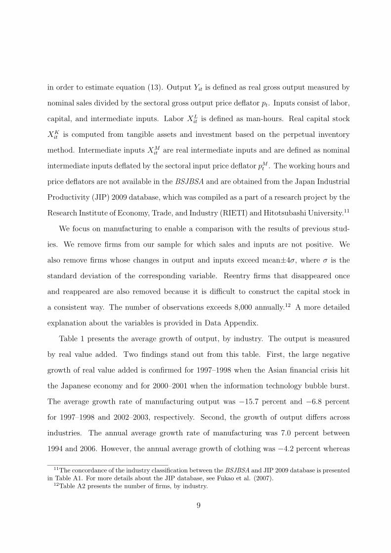
Table 1 presents the average growth of output, by industry. The output is measured

by real value added. Two findings stand out from this table. First, the large negative

growth of real value added is confirmed for 1997–1998 when the Asian financial crisis hit

the Japanese economy and for 2000–2001 when the information technology bubble burst.

The average growth rate of manufacturing output was −15.7 percent and −6.8 percent

for 1997–1998 and 2002–2003, respectively. Second, the growth of output differs across

industries. The annual average growth rate of manufacturing was 7.0 percent between

1994 and 2006. However, the annual average growth of clothing was −4.2 percent whereas

11The concordance of the industry classification between the BSJBSA and JIP 2009 database is presentedin Table A1. For more details about the JIP database, see Fukao et al. (2007).

12Table A2 presents the number of firms, by industry.

9

that of electronic parts and components was 15.4 percent. These results together suggest

that the growth of output is heterogeneous across years and across industries.

=== Table 1 ===

4 Productivity, Markup, Scale Economies, and the

Business Cycle

4.1 Do sectoral productivity, markup, and scale economies cor-

relate with the business cycle?

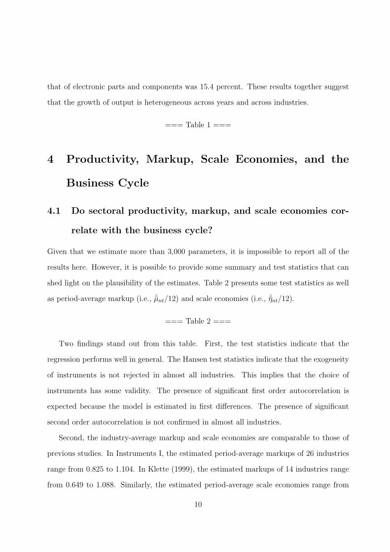
Given that we estimate more than 3,000 parameters, it is impossible to report all of the

results here. However, it is possible to provide some summary and test statistics that can

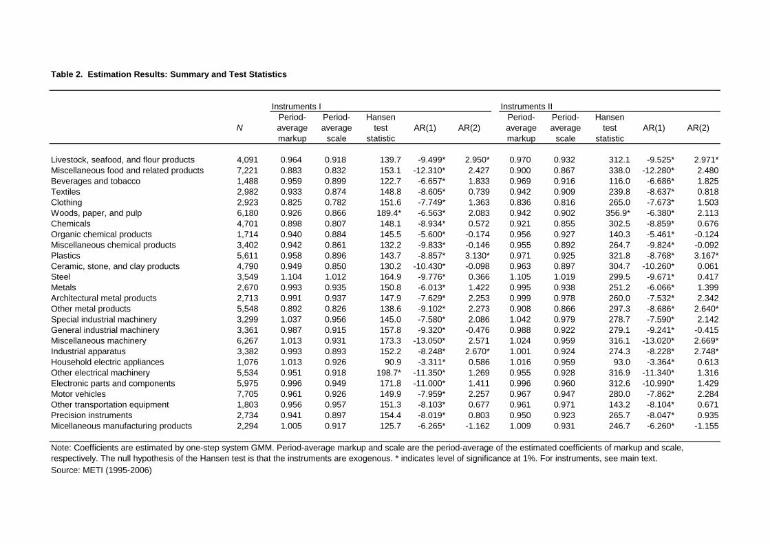
shed light on the plausibility of the estimates. Table 2 presents some test statistics as well

as period-average markup (i.e., ˆµnt/12) and scale economies (i.e., ˆηnt/12).

=== Table 2 ===

Two findings stand out from this table. First, the test statistics indicate that the

regression performs well in general. The Hansen test statistics indicate that the exogeneity

of instruments is not rejected in almost all industries. This implies that the choice of

instruments has some validity. The presence of significant first order autocorrelation is

expected because the model is estimated in first differences. The presence of significant

second order autocorrelation is not confirmed in almost all industries.

Second, the industry-average markup and scale economies are comparable to those of

previous studies. In Instruments I, the estimated period-average markups of 26 industries

range from 0.825 to 1.104. In Klette (1999), the estimated markups of 14 industries range

from 0.649 to 1.088. Similarly, the estimated period-average scale economies range from

10

0.782 to 1.012, while those of Klette (1999) range from 0.653 to 1.009. Quantitatively

similar results are obtained when we use Instruments II. These results show the plausibility

of the estimates.

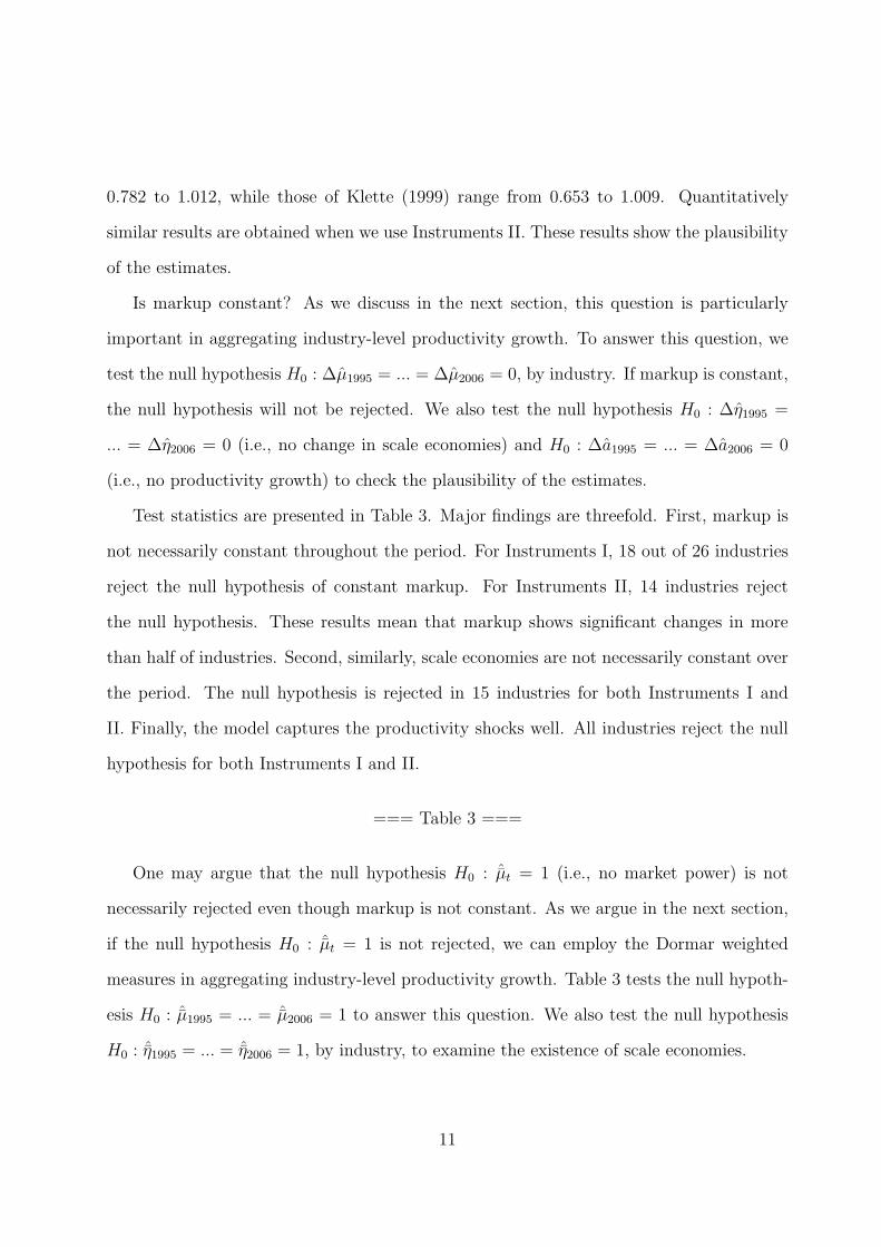
Is markup constant? As we discuss in the next section, this question is particularly

important in aggregating industry-level productivity growth. To answer this question, we

test the null hypothesis H0 : ∆µ1995 = ... = ∆µ2006 = 0, by industry. If markup is constant,

the null hypothesis will not be rejected. We also test the null hypothesis H0 : ∆η1995 =

... = ∆η2006 = 0 (i.e., no change in scale economies) and H0 : ∆a1995 = ... = ∆a2006 = 0

(i.e., no productivity growth) to check the plausibility of the estimates.

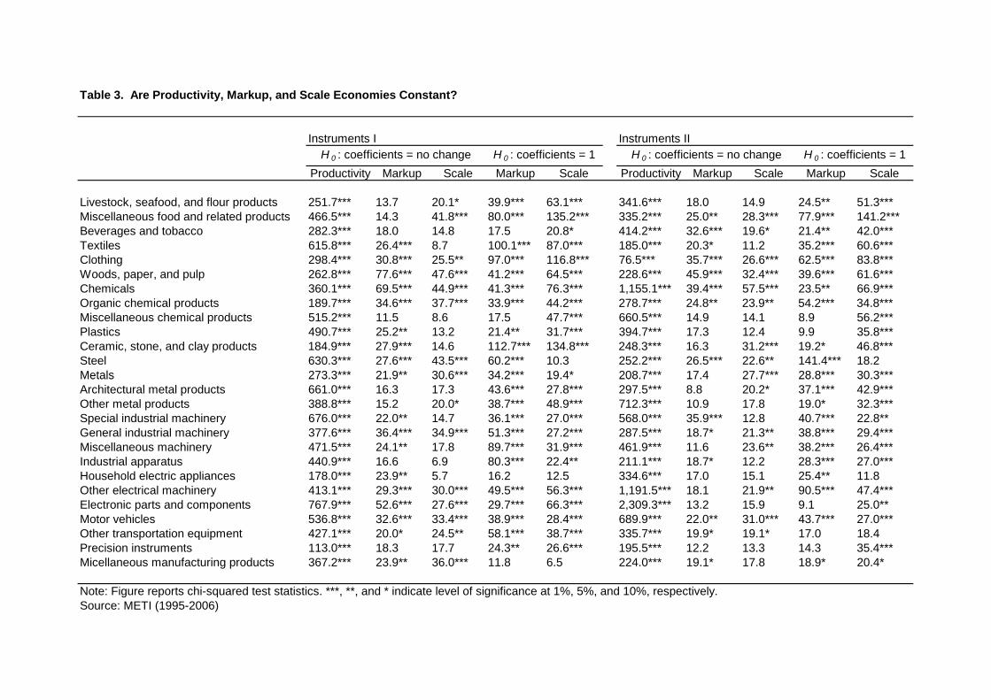
Test statistics are presented in Table 3. Major findings are threefold. First, markup is

not necessarily constant throughout the period. For Instruments I, 18 out of 26 industries

reject the null hypothesis of constant markup. For Instruments II, 14 industries reject

the null hypothesis. These results mean that markup shows significant changes in more

than half of industries. Second, similarly, scale economies are not necessarily constant over

the period. The null hypothesis is rejected in 15 industries for both Instruments I and

II. Finally, the model captures the productivity shocks well. All industries reject the null

hypothesis for both Instruments I and II.

=== Table 3 ===

One may argue that the null hypothesis H0 : ˆµt = 1 (i.e., no market power) is not

necessarily rejected even though markup is not constant. As we argue in the next section,

if the null hypothesis H0 : ˆµt = 1 is not rejected, we can employ the Dormar weighted

measures in aggregating industry-level productivity growth. Table 3 tests the null hypoth-

esis H0 : ˆµ1995 = ... = ˆµ2006 = 1 to answer this question. We also test the null hypothesis

H0 : ˆη1995 = ... = ˆη2006 = 1, by industry, to examine the existence of scale economies.

11

The results indicate that the hypothesis H0 : ˆµ1995 = ... = ˆµ2006 = 1 is not supported in

the majority of industries. For Instruments I, the null hypothesis is rejected in 22 out of 26

industries. Similarly, Table 3 does not support constant returns to scale. For Instruments

I, the null hypothesis H0 : ˆη1995 = ... = ˆη2006 = 1 is rejected in 23 out of 26 industries.

Quantitatively similar results are obtained for Instruments II.

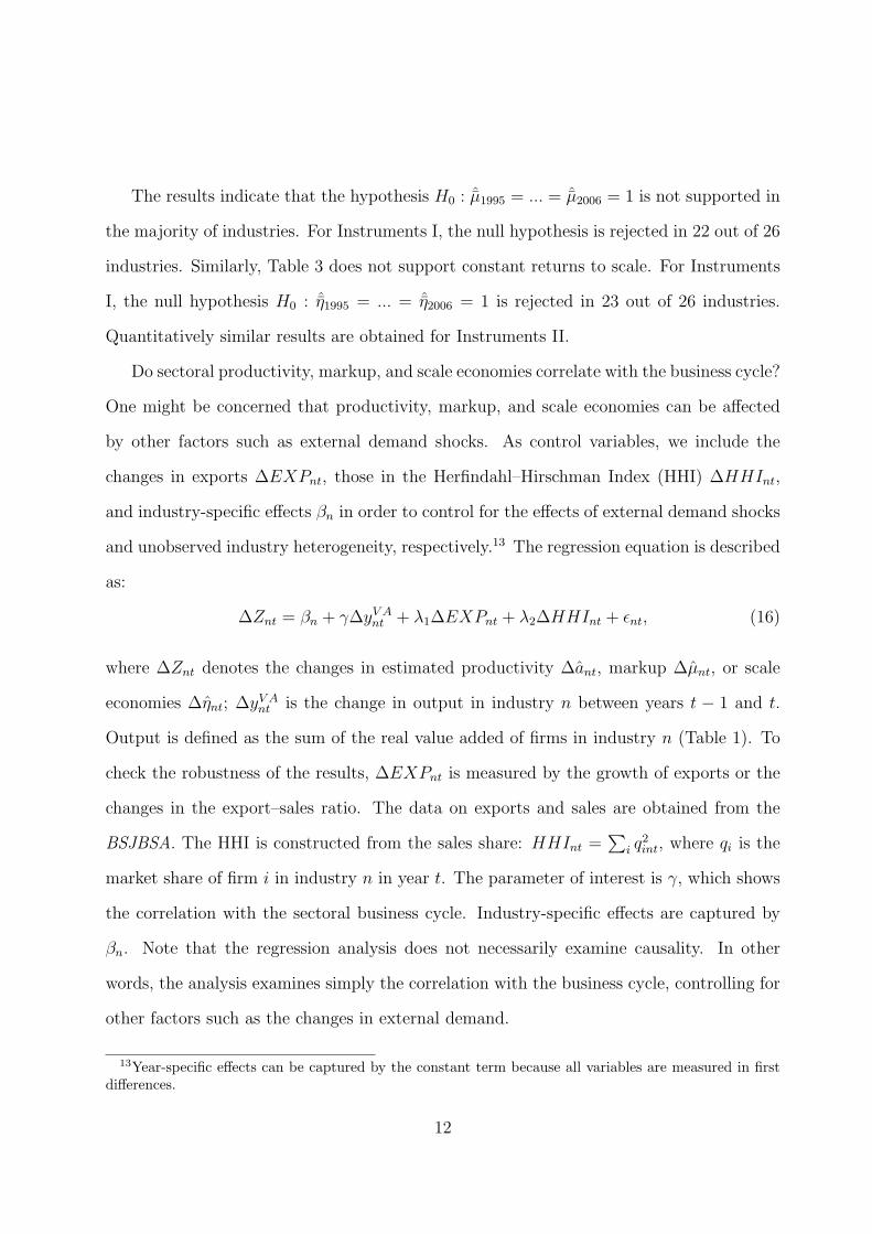
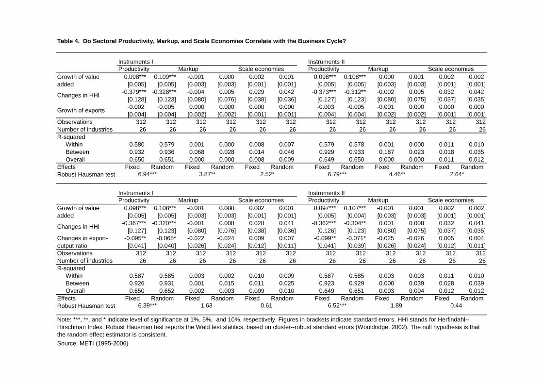
Do sectoral productivity, markup, and scale economies correlate with the business cycle?

One might be concerned that productivity, markup, and scale economies can be affected

by other factors such as external demand shocks. As control variables, we include the

changes in exports ∆EXPnt, those in the Herfindahl–Hirschman Index (HHI) ∆HHInt,

and industry-specific effects βn in order to control for the effects of external demand shocks

and unobserved industry heterogeneity, respectively.13 The regression equation is described

as:

∆Znt = βn + γ∆yV Ant + λ1∆EXPnt + λ2∆HHInt + ϵnt, (16)

where ∆Znt denotes the changes in estimated productivity ∆ant, markup ∆µnt, or scale

economies ∆ηnt; ∆yV Ant is the change in output in industry n between years t − 1 and t.

Output is defined as the sum of the real value added of firms in industry n (Table 1). To

check the robustness of the results, ∆EXPnt is measured by the growth of exports or the

changes in the export–sales ratio. The data on exports and sales are obtained from the

BSJBSA. The HHI is constructed from the sales share: HHInt =∑

i q2int, where qi is the

market share of firm i in industry n in year t. The parameter of interest is γ, which shows

the correlation with the sectoral business cycle. Industry-specific effects are captured by

βn. Note that the regression analysis does not necessarily examine causality. In other

words, the analysis examines simply the correlation with the business cycle, controlling for

other factors such as the changes in external demand.

13Year-specific effects can be captured by the constant term because all variables are measured in firstdifferences.

12

=== Table 4 ===

Table 4 shows the regression results. The results indicate that the coefficients of the

changes in output are significantly positive for the changes in productivity. The result sug-

gests that the productivity growth is procyclical, which supports the finding of Miyagawa

et al. (2006), who found procyclical movement of productivity in Japan. In contrast, the

coefficients of the changes in output are insignificant for the changes in markup. This find-

ing suggests that markup is neither procyclical nor countercyclical. This result contradicts

the findings of Nishimura et al. (1999) and Kiyota et al. (2009), who found procyclical

movement of markup in Japan. The relationship between scale economies and the business

cycle is also insignificant.

The procyclical movement of productivity is confirmed even after changes in each vari-

able are controlled for. However, the procyclical movement of markup disappears once the

changes in productivity are taken into account. The results imply that previous studies

may thus misinterpret the movement of procyclical productivity as procyclical markup.

The changes in exports are generally insignificant. Besides, this result holds whether the

changes in exports are measured by the growth of exports or the changes in the export–sales

ratio. This result suggests that the effects of external demand on productivity, markup,

and scale economies may be limited in this period. The changes in HHI have significantly

negative coefficients for productivity growth. This result means that productivity growth

declines with increases in the industry’s concentration. In other words, productivity growth

is enhanced in competitive markets. In contrast, the changes in HHI do not show any

significant coefficients for markup. Further analysis is needed to clarify the determinants

of changes in markup.

13

4.2 Is aggregate productivity procyclical?

Is aggregate productivity procyclical? The estimation results in the previous section are

not able to answer this question directly because productivity growth is estimated at the

industry level. Note also that the previous section focuses on industry-average productivity

growth. If productivity growth is different between large and small industries, the growth

of aggregate productivity can show a different pattern from that of industry-average pro-

ductivity. To aggregate the sectoral productivity growth, this paper utilizes the markup

corrected measures developed by Basu and Fernald (2001).

Denote changes in aggregate productivity as ∆aAt . Reintroduce industry subscript n.

Define aggregate productivity growth ∆aAt as a weighted average of industry productivity

growth:

∆aAt =

∑n

(sV A

nt

1 − ˆµntsMnt

)∆ant, (17)

where ∆ant is the estimated productivity growth of industry n from equation (13); ˆµnt is

the estimated markup of industry n from equation (13); and sV Ant is the share of industry

n’s value added between years t and t − 1:

sV Ant =

sV Ant + sV A

nt−1

2, sM

nt =sM

nt + sMnt−1

2, sV A

nt =pntYnt − pM

ntXMnt∑

n(pntYnt − pMntX

Mnt )

,

pntYnt =∑i∈n

pitYit, and pMntX

Mnt =

∑i∈n

pMit XM

it . (18)

The estimated industry productivity changes are first divided by 1 − ˆµntsMnt in order to

convert them from a gross output to a value-added basis. These changes are weighted by

the industry’s share of aggregate value added.14

Note that this aggregation scheme does not include the contribution of entry and exit

because growth is defined for firms that exist between years t and t−1. However, Nishimura

14Under perfect competition, ˆµnt = 1. This is known as the Domar weighted measure (Domar, 1961).

14

et al. (2005) used the same firm-level data for 1994–1998 and found that the effects of net

entry (= entry − exit) on aggregate productivity growth were rather small. A similar

finding is confirmed in Fukao and Kwon (2006). Although the effects of entry and exit

could be substantial in other countries where entry and exit are active, they are marginal

during the sample period in Japan.

For equation (17), a number of studies assumed that markup was constant over their

sample period: ˆµnt = ˆµn, or that markup was equal to unity: ˆµnt = 1. However, the estima-

tion results of the previous section questioned the empirical validity of these assumptions.

The results suggest that one needs the parameters of markup by year and by industry in

order to utilize the markup corrected measures. More careful treatment is thus needed in

using the markup corrected measures. Unlike previous studies, the analysis in this paper

takes into account the changes in markup.

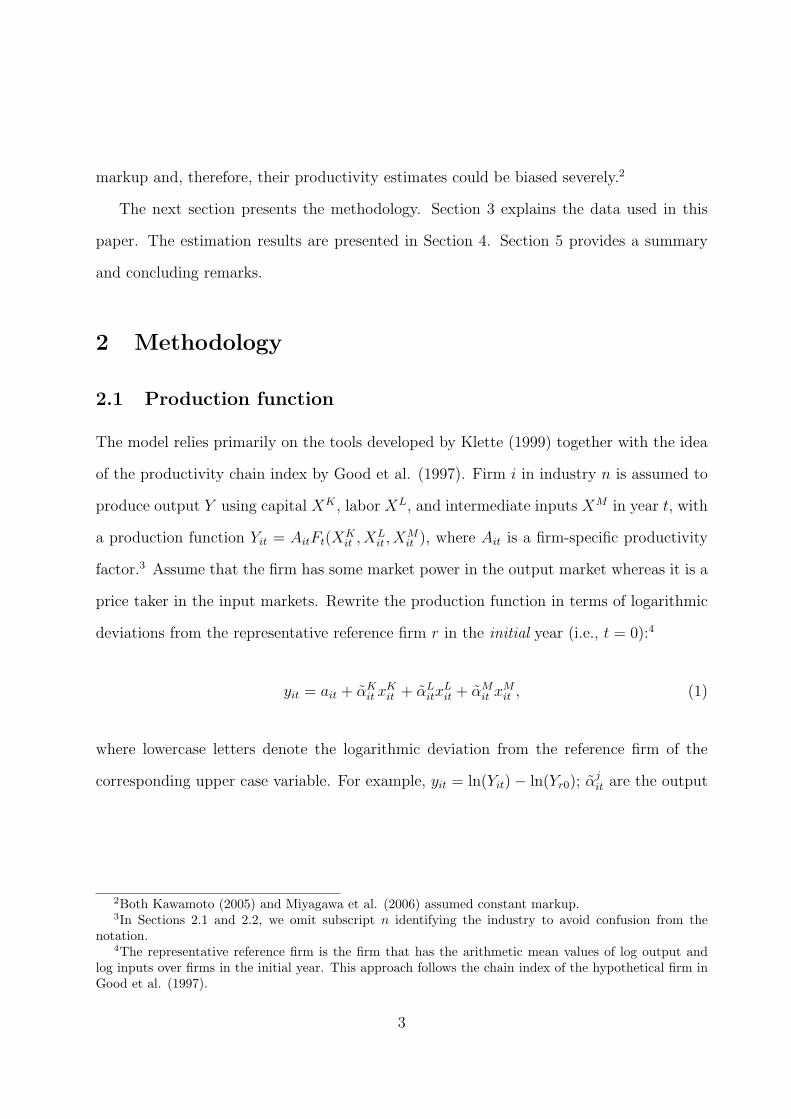
Figure 1 presents the results. The business cycle is measured by the growth of real

value added in manufacturing. Figure 1 indicates that aggregate productivity is procyclical.

Indeed, the correlation coefficients between aggregate productivity and the business cycle

are 0.90 for both Instruments I and II.15 The results suggest that aggregate productivity is

also procyclical even after the changes in markup and scale economies are controlled for.

=== Figure 1 ===

One may be concerned that the business cycle can be measured in alternative ways.

For example, the Bank of Japan (BOJ) conducts a statistical survey called TANKAN

(the Short-term Economic Survey of Enterprises in Japan) to capture the business trends

of enterprises in Japan. Similarly, the METI surveys business conditions monthly and

constructs the indices of industrial production and producers’ shipments. These indices

may be more appropriate for measuring the business cycle than changes in output.

15The correlation of aggregate productivity between Instruments I and II is 0.9986.

15

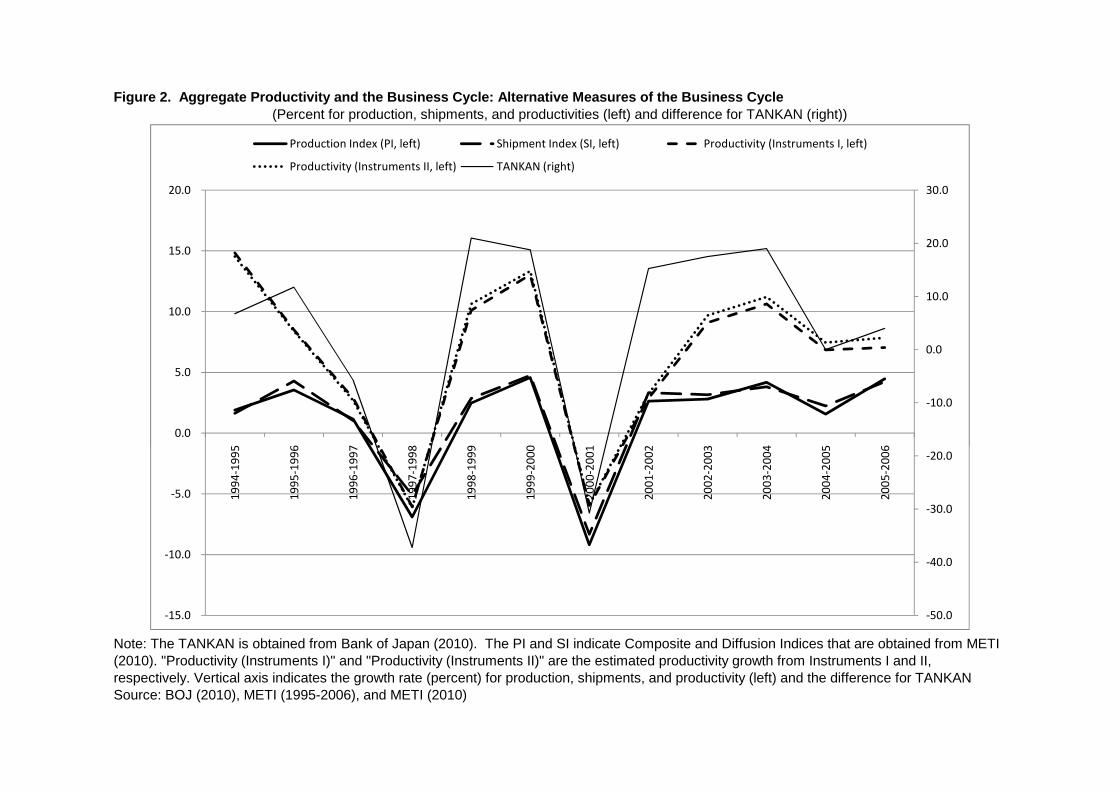
To address this concern, we also examine how the results are sensitive to the measure-

ment of the business cycle. Three alternative measures are used in this paper: 1) TANKAN,

2) index of industrial production, or production index (PI), and 3) index of producers’ ship-

ments, or shipments index (SI). The TANKAN is obtained from the Bank of Japan (2010)

while both PI and SI are obtained from METI (2010).16 Note that the TANKAN is sur-

veyed quarterly and the PI and SI are surveyed monthly. For the TANKAN, we first

calculate the annual average indices (fiscal year basis) and then take the first differences

between two consecutive years to compare with annual growth of aggregate productivity.17

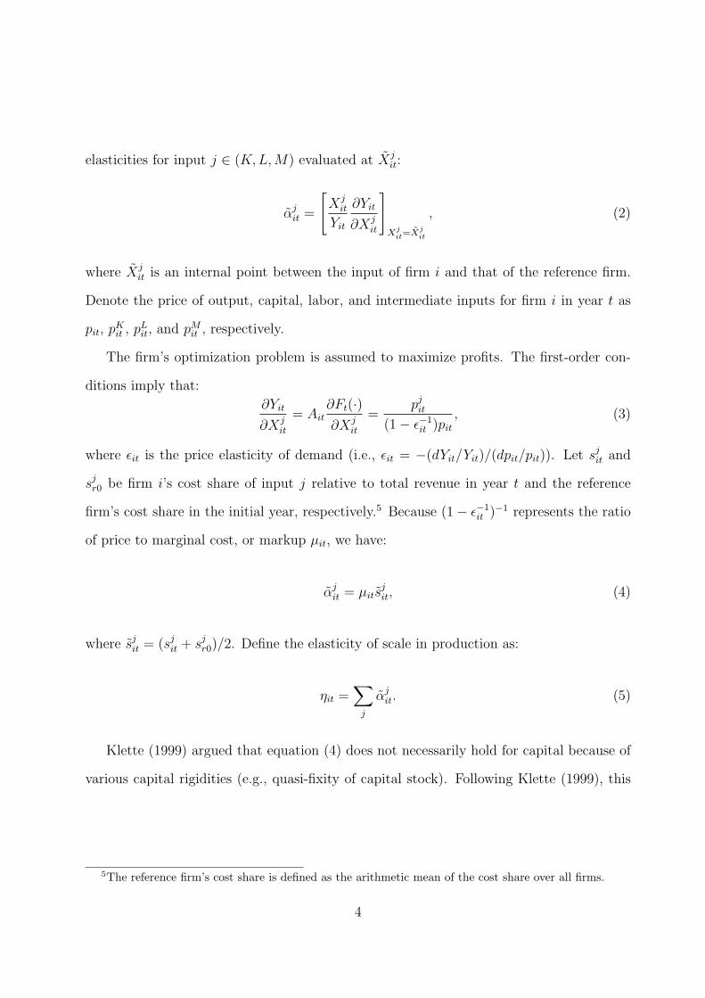
Figure 2 presents the results. The results indicate that the procyclical movement of ag-

gregate productivity is confirmed even when we utilize the different measures of the business

cycle. The correlation coefficients between aggregate productivity and the TANKAN are

0.87 and 0.88 for Instruments I and II, respectively. Similarly, the correlation coefficients

between aggregate productivity and PI are 0.86 and 0.87 for Instruments I and II, respec-

tively, while those between aggregate productivity and SI are 0.84 and 0.85 for Instruments

I and II, respectively. These results together suggest that the procyclicality of productivity

is not sensitive to the measurement of the business cycle.

=== Figure 2 ===

5 Concluding Remarks

This paper asked two questions: 1) Do sectoral productivity, markup, and scale economies

correlate with the business cycle? 2) Is aggregate productivity procyclical? A contribution

of this paper is to present a simple econometric framework that permits simultaneous

estimation of the changes in productivity, markup, and scale economies from a panel of

firm-level data. The framework is then applied to Japanese firm-level data for 1994–2006.16Both PI and SI are seasonally adjusted indices.17We calculate the first difference rather than the growth rate because these indices take negative values.

16

The major findings of this paper are threefold. First, markup is not necessarily constant

over the period. The null hypothesis that markup is constant is rejected in more than

half of industries. The result implies that more careful treatment is needed in using the

markup corrected measures to aggregate productivity growth because previous studies have

assumed that markup is constant over the period.

Second, productivity shows procyclical movement. The relationship between sectoral

value-added growth and sectoral productivity growth is significantly positive. At the aggre-

gate level, the correlation coefficient between productivity and the business cycle, measured

by aggregate real value added, is around 0.9. These results together imply that produc-

tivity is procyclical even after the changes in markup and scale economies are controlled

for.

Third, however, markup and scale economies are neither procyclical nor countercyclical

once changes in productivity are taken into account. At the sectoral level, the correlation

between markup and the business cycle as well as the correlation between scale economies

and the business cycle are insignificant. Insignificant correlation between markup and

the business cycle contradicts the findings of Nishimura et al. (1999) and Kiyota et al.

(2009), who found procyclical movement of markup in Japan. Previous studies thus may

misinterpret the movement of procyclical productivity as procyclical markup.

The results of this paper also shed light on the importance of studies that utilize firm-

level data in both industry- and aggregate-level analysis. A study utilizing industry-level

data may not be able to estimate markup or scale economies by year and by industry

because the number of parameters will exceed the number of observations. To clarify the

relationship between productivity and the business cycle, therefore, it is imperative that

the quality and coverage of the firm-level data be improved and expanded.

In conclusion, there are several research issues for the future that are worth mentioning.

First, the analysis that utilized firm-level data in other countries is an important extension.

17

This paper found that the procyclical movement of markup disappears once the changes in

productivity are controlled for. This result suggests that the observed procyclical movement

of markup in other countries is likely to overstate the changes in markup.

Second, further investigation of the relationship between productivity, markup, and the

business cycle is an important extension. For example, this paper utilized annual data.

However, quarterly or monthly data might be more appropriate for capturing the business

cycle. To conduct a more detailed analysis, more detailed firm-level data can be helpful.

Finally, it is also important to examine the determinants of changes in markup, pro-

ductivity, and scale economies in more detail. A study using data on different countries

and/or periods will add a national perspective to the growing body of empirical literature

on productivity, markup, and the business cycle. Although this paper found procyclical

movement of markup in Japan, different patterns may be confirmed in other countries.

These issues will be addressed in our future research.

Data Appendix

Output is defined as total sales divided by the gross output price index. Total sales are

available in the Basic Survey of Japanese Business Structure and Activities (BSJBSA). The

gross output price index is obtained from the JIP 2009 database and defined as sectoral

nominal gross output divided by sectoral real gross output (2000 constant prices).

Intermediate inputs are defined as nominal intermediate inputs divided by the input

price index. Data for the nominal intermediate inputs are available in the BSJBSA and

defined as: operating cost (= sales cost + administrative cost) − (wage payments + depre-

ciation cost). The input price index is obtained from the JIP 2009 database and defined

as sectoral nominal intermediate inputs divided by sectoral real intermediate inputs.

Labor input is defined as number of man-hours, which is each firm’s total number of

18

workers multiplied by working hours. The total number of regular workers is obtained from

the BSJBSA. Because working hours are not available in the BSJBSA, we obtain sectoral

annual average working hours from the JIP 2009 database and multiply it by the number

of regular workers.

Capital stock is constructed from tangible fixed assets. In the BSJBSA, tangible fixed

assets include land that is reported at nominal book values except for 1995 and 1996. In

other words, the information on land is available only in 1995 and 1996. To construct

capital stock, we first exclude land from tangible fixed assets, multiplying by (1 − land

ratio):

BKit = BK

it × (1 − ξ), (A-1)

where BKit and BK

it are the book value of tangible fixed assets that exclude land and include

land, respectively, and ξ is the land ratio. For the land ratio, following Fukao and Kwon

(2006), we use the industry-average ratio of land to tangible fixed assets in 1995 and 1996.18

The book value of tangible assets (excluding land) is then converted to the current

value of, or nominal, tangible assets. The conversion rate is constructed from Financial

Statements Statistics of Corporations by Industry published by the Ministry of Finance.

The value of nominal tangible assets is then deflated by the investment goods deflator:

XKit =

BKit × ρt

pIt

, (A-2)

where XKit denotes real tangible assets for firm i in year t (2000 constant prices); ρt is the

conversion rate;19 and pIt is the investment goods deflator. The real value of tangible assets

in the initial year τ (τ is 1994 or the first year when a firm appeared in the BSJBSA) is

defined as the initial capital stock: XKiτ . Then the perpetual inventory method is used to

18Therefore, the land ratio is constant throughout the period.19For more details about the conversion rate, see Tokui, Inui, and Kim (2008).

19

construct real capital stock:

XKit = XK

it−1(1 − δt) + XIit/p

It , (A-3)

where XKit is the capital stock for firm i in year t; δt is the depreciation rate; XI

it is

investment; and pIt is the investment goods deflator.20 The depreciation rate is defined

as the weighted average of various assets in an industry. The investment goods deflator

is defined as sectoral nominal investment flows divided by sectoral real investment flows.

Both the depreciation rate and the investment goods deflator are obtained from the JIP

2009 database.

The cost of intermediate inputs is defined as nominal intermediate inputs while that of

labor is wage payments. The cost of capital is the user cost of capital multiplied by the

real capital stock. The user cost of capital is obtained from the JIP 2009 database and

defined as the sectoral nominal capital cost divided by the sectoral real capital stock.

Exports are also available at the firm level in the BSJBSA. One problem is that the

definition of exports in the BSJBSA changed in 1997. Before 1997, exports included sales

by foreign branches (indirect exports). After 1997, however, exports are defined as exports

from the parent firm (direct exports). Total (direct plus indirect) exports are also available

between 1997 and 1999. For consistency, this paper focuses on direct exports. Exports

before 1997 are adjusted by multiplying the figure by the ratio of direct exports to total

exports. The ratio of direct exports is defined as the industry-average ratio of direct exports

to total exports between 1997 and 1999.

Note that the industry classification of the BSJBSA is not the same as that of the JIP

2009 database. If one industry in the BSJBSA corresponds to more than one industry

in the JIP 2009 database, we aggregate the nominal values and real values from the JIP

20We regard firms that did not report investment as firms with no investment (zero investment).

20

2009 database and then divide the aggregate nominal values by the aggregate real values

to obtain indices. The concordance of the industry classification between the BSJBSA and

the JIP 2009 database is presented in Table A1.

In constructing these variables, some firms report unusual figures. This paper 1) selects

manufacturing; 2) removes firms whose sales and inputs were not positive; 3) removes

firms whose changes in output ∆yit and inputs ∆xVit and ∆xK

it exceed mean±4σ, where

σ is the standard deviation of the corresponding variable; and 4) removes reentry firms

that disappear once and reappear, because it is difficult to construct the capital stock

in a consistent way. As Table A2 shows, the total number of observations exceeds 8,000

annually.

References

Arellano, Manuel and Stephen Bond (1991) “Some Tests of Specification for Panel Data:

Monte Carlo Evidence and an Application to Employment Equations,” Review of

Economic Studies, 58(2): 277–297.

Baltagi, Badi H. (2005) Econometric Analysis of Panel Data, 3rd Ed., Chichester, UK:

John Wiley & Sons.

Bank of Japan (BOJ) (2010) TANKAN (The Short-Term Survey of Enterprises in Japan),

Tokyo: BOJ website.

Basu, Susanto (1996) “Procyclical Productivity: Increasing Returns to Scale or Cyclical

Utilization,” Quarterly Journal of Economics, 111(3): 719–751.

Basu, Susanto and John G. Fernald (1997) “Returns to Scale in U.S. Production: Estimates

and Implications,” Journal of Political Economy, 105(2): 249–283.

Basu, Susanto and John G. Fernald (2001) “Why Is Productivity Procyclical? Why Do

21

We Care?” in Charles R. Hulten, Edwin R. Dean, and Michael J. Harper (eds.),

New Developments in Productivity Analysis, Chicago, IL: University of Chicago

Press/NBER, 225–301.

Beccarello, Massimo (1996) “Time Series Analysis of Market Power: Evidence from G-7

Manufacturing,” International Journal of Industrial Organization, 15(1): 123–136.

Blundell, Richard and Stephen Bond (1998) “Initial Conditions and Moment Restrictions

in Dynamic Panel Data Models,” Journal of Econometrics, 87(1): 115–143.

Bottasso, Anna and Alessandro Sembenelli (2001) “Market Power, Productivity and the

EU Single Market Program: Evidence from a Panel of Intalian Firms,” European

Economic Review, 45(1): 167–186.

Chevalier, Judith A. and David S. Scharfstein (1996) “Capital-Market Imperfections and

Countercyclical Markups: Theory and Evidence,” American Economic Review,

86(4): 703–725.

Domar, Evsey D. (1961) “On the Measurement of Technical Change,” Economic Journal,

71(284): 710–729.

Fukao, Kyoji, Sumio Hamagata, Tomohiko Inui, Keiko Ito, Hyeog Ug Kwon, Tatsuji

Makino, Tsutomu Miyagawa, Yasuo Nakanishi, and Joji Tokui (2007) “Estima-

tion Procedures and TFP Analysis of the JIP Database 2006,” RIETI Discussion

Paper, 07-E-003.

Fukao, Kyoji and Hyeog Ug Kwon (2006) “Why Did Japan’s TFP Growth Slow Down in the

Lost Decade? An Empirical Analysis Based on Firm-Level Data of Manufacturing,”

Japanese Economic Review, 57(2): 195–228.

Good, David H., M. Ishaq Nadiri, and Robin Sickles (1997) “Index Number and Factor

Demand Approaches to the Estimation of Productivity,” in M. Hashem Pesaran and

22

Peter Schmidt (eds.), Handbook of Applied Econometrics: Microeconometrics, Vol.

II., Oxford: Blackwell.

Hayashi, Fumio and Edward C. Prescott (2002) “The 1990s in Japan: A Lost Decade,”

Review of Economic Dynamics, 5(1): 206–235.

Inklaar, Robert (2007) “Cyclical Productivity in Europe and the United States: Evaluating

the Evidence on Returns to Scale and Input Utilization,” Economica, 74(296): 822–

841.

Kawamoto, Takuji (2005) “What Do the Purified Solow Residuals Tell Us about Japan’s

Lost Decade?” Monetary and Economic Studies, 23(1): 113–148.

Kiyota, Kozo, Takanobu Nakajima, and Kiyohiko G. Nishimura (2009) “Measurement of

the Market Power of Firms: The Japanese Case in the 1990s,” Industrial and Cor-

porate Change, 18(3): 381–414.

Klette, Tor Jacob (1999) “Market Power, Scale Economies and Productivity: Estimates

from a Panel of Establishment Data,” Journal of Industrial Economics, 47(4): 451–

476.

Miyagawa, Tsutomu, Yukie Sakuragawa, and Miho Takizawa (2006) “Productivity and

Business Cycles in Japan: Evidence from Japanese Industry Data,” Japanese Eco-

nomic Review, 57(2): 161–186.

Nishimura, Kiyohiko G., Takanobu Nakajima, and Kozo Kiyota (2005) “Does the Natural

Selection Mechanism Still Work in Severe Recessions? Examination of the Japanese

Economy in the 1990s,” Journal of Economic Behavior and Organization, 58(1):

53–78.

Nishimura, Kiyohiko G., Yasushi Ohkusa, and Kenn Ariga (1999) “Estimating the Mark-up

Over Marginal Cost: A Panel Analysis of Japanese Firms 1971–1994,” International

Journal of Industrial Organization, 17(8): 1077–1111.

23

Research and Statistics Department, Ministry of Economy, Trade and Industry (METI)

(1994–2006) Kigyou Katsudou Kihon Chousa Houkokusho (Basic Survey of Japanese

Business Structure and Activities), Tokyo: METI.

Research and Statistics Department, Ministry of Economy, Trade and Industry (METI)

(2010) Kokogyou Seisan Shisuu (Indices on Mining and Manufacturing), Tokyo:

METI website.

Rotemberg, Julio J. and Michael Woodford (1991) “Markups and the Business Cycle,”

NBER Macroeconomics Annual 1991, 6: 63–129.

Tokui, Joji, Tomohiko Inui, and Young Gak Kim (2008) “Embodied Technological Progress

and Productivity Slowdown in Japan,” RIETI Discussion Paper Series 08-E-017,

Research Institute of Economy, Trade, and Industry.

Van Biesebroeck, Johannes (2007) “Robustness of Productivity Estimates,” Journal of

Industrial Economics, 55(3): 529–569.

Wooldridge, Jeffrey M. (2002) Econometric Analysis of Cross Section and Panel Data,

Cambridge, MA: MIT Press.

24

5.0 

10.0 

15.0 

20.0 

25.0 

30.0 

Value added Productivity (Instruments I) Productivity (Instruments II)

truments II)" are the estimated

Figure 1. Is Aggregate Productivity Pro-cyclical?(Percent)

Note: Value added indicates the growth of real value added. "Productivity (Instruments I)" and "Productivity (Insproductivity growth from Instruments I and II, respectively. Vertical axis indicates the growth rate (percent).Source: METI (1995-2006)

‐20.0 

‐15.0 

‐10.0 

‐5.0 

0.0 

5.0 

10.0 

15.0 

20.0 

25.0 

30.0 

1994

‐1995

1995

‐1996

1996

‐1997

1997

‐1998

1998

‐1999

1999

‐2000

2000

‐2001

2001

‐2002

2002

‐2003

2003

‐2004

2004

‐2005

2005

‐2006

Value added Productivity (Instruments I) Productivity (Instruments II)

‐10.0 

0.0 

10.0 

20.0 

30.0 

0.0 

5.0 

10.0 

15.0 

20.0 

5 6 7 8 9 0 1 2 3 4 5 6

Production Index (PI, left) Shipment Index (SI, left) Productivity (Instruments I, left)

Productivity (Instruments II, left) TANKAN (right)

es that are obtained from METI Instruments I and II,

ference for TANKAN

Figure 2. Aggregate Productivity and the Business Cycle: Alternative Measures of the Business Cycle(Percent for production, shipments, and productivities (left) and difference for TANKAN (right))

Note: The TANKAN is obtained from Bank of Japan (2010). The PI and SI indicate Composite and Diffusion Indic(2010). "Productivity (Instruments I)" and "Productivity (Instruments II)" are the estimated productivity growth fromrespectively. Vertical axis indicates the growth rate (percent) for production, shipments, and productivity (left) and the difSource: BOJ (2010), METI (1995-2006), and METI (2010)

‐50.0 

‐40.0 

‐30.0 

‐20.0 

‐10.0 

0.0 

10.0 

20.0 

30.0 

‐15.0 

‐10.0 

‐5.0 

0.0 

5.0 

10.0 

15.0 

20.0 

1994

‐1995

1995

‐1996

1996

‐1997

1997

‐1998

1998

‐1999

1999

‐2000

2000

‐2001

2001

‐2002

2002

‐2003

2003

‐2004

2004

‐2005

2005

‐2006

Production Index (PI, left) Shipment Index (SI, left) Productivity (Instruments I, left)

Productivity (Instruments II, left) TANKAN (right)

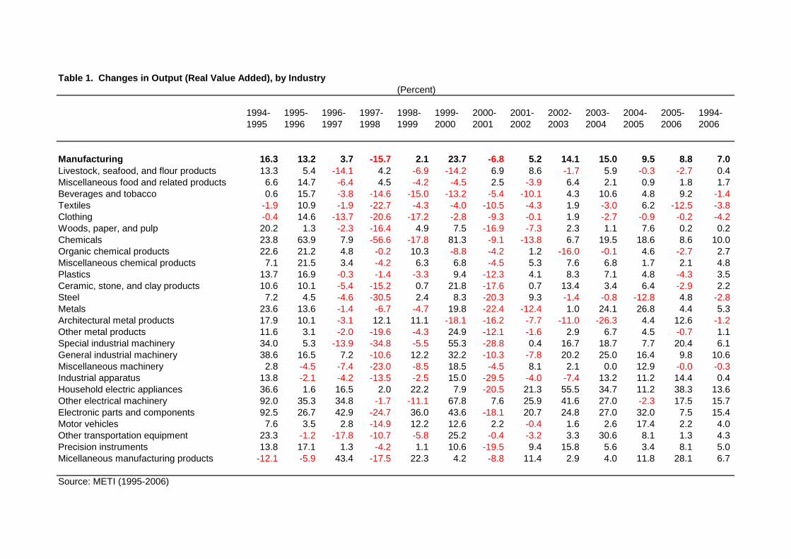
Table 1. Changes in Output (Real Value Added), by Industry(Percent)

1919

94-95

1995-1996

199199

6-7

11997-998

1998-1999

199200

9-0

22000-001

2001-2002

2002-2003

2003-2004

2004-2005

2005-2006

1994-2006

Manufacturing 16.3 13.2 3.7 -15.7 2.1 23.7 -6.8 5.2 14.1 15.0 9.5 8.8 7.0Livestock, seafood, and flour products 13.3 5.4 -14.1 4.2 -6.9 -14.2 6.9 8.6 -1.7 5.9 -0.3 -2.7 0.4Miscellaneous food and related products 6.6 14.7 -6.4 4.5 -4.2 -4.5 2.5 -3.9 6.4 2.1 0.9 1.8 1.7Beverages and tobacco 0.6 15.7 -3.8 -14.6 -15.0 -13.2 -5.4 -10.1 4.3 10.6 4.8 9.2 -1.4 Textiles -1.9 10.9 -1.9 -22.7 -4.3 -4.0 -10.5 -4.3 1.9 -3.0 6.2 -12.5 -3.8 Clothing -0.4 14.6 -13.7 -20.6 -17.2 -2.8 -9.3 -0.1 1.9 -2.7 -0.9 -0.2 -4.2 Woods, paper, and pulp 20.2 1.3 -2.3 -16.4 4.9 7.5 -16.9 -7.3 2.3 1.1 7.6 0.2 0.2Chemicals 23.8 63.9 7.9 -56.6 -17.8 81.3 -9.1 -13.8 6.7 19.5 18.6 8.6 10.0Organic chemical products 22.6 21.2 4.8 -0.2 10.3 -8.8 -4.2 1.2 -16.0 -0.1 4.6 -2.7 2.7Miscellaneous chemical products 7.1 21.5 3.4 -4.2 6.3 6.8 -4.5 5.3 7.6 6.8 1.7 2.1 4.8Plastics 13.7 16.9 -0.3 -1.4 -3.3 9.4 -12.3 4.1 8.3 7.1 4.8 -4.3 3.5Ceramic, stone, and clay products 10.6 10.1 -5.4 -15.2 0.7 21.8 -17.6 0.7 13.4 3.4 6.4 -2.9 2.2Steel 7.2 4.5 -4.6 -30.5 2.4 8.3 -20.3 9.3 -1.4 -0.8 -12.8 4.8 -2.8 Metals 23.6 13.6 -1.4 -6.7 -4.7 19.8 -22.4 -12.4 1.0 24.1 26.8 4.4 5.3Architectural metal products 17.9 10.1 -3.1 12.1 11.1 -18.1 -16.2 -7.7 -11.0 -26.3 4.4 12.6 -1.2 Other metal products 11.6 3.1 -2.0 -19.6 -4.3 24.9 -12.1 -1.6 2.9 6.7 4.5 -0.7 1.1Special industrial machinery 34.0 5.3 -13.9 -34.8 -5.5 55.3 -28.8 0.4 16.7 18.7 7.7 20.4 6.1General industrial machinery 38.6 16.5 7.2 -10.6 12.2 32.2 -10.3 -7.8 20.2 25.0 16.4 9.8 10.6Miscellaneous machinery 2.8 -4.5 -7.4 -23.0 -8.5 18.5 -4.5 8.1 2.1 0.0 12.9 -0.0 -0.3 Industrial apparatus 13.8 -2.1 -4.2 -13.5 -2.5 15.0 -29.5 -4.0 -7.4 13.2 11.2 14.4 0.4Household electric appliances 36.6 1.6 16.5 2.0 22.2 7.9 -20.5 21.3 55.5 34.7 11.2 38.3 13.6Other electrical machinery 92.0 35.3 34.8 -1.7 -11.1 67.8 7.6 25.9 41.6 27.0 -2.3 17.5 15.7Electronic parts and components 92.5 26.7 42.9 -24.7 36.0 43.6 -18.1 20.7 24.8 27.0 32.0 7.5 15.4Motor vehicles 7.6 3.5 2.8 -14.9 12.2 12.6 2.2 -0.4 1.6 2.6 17.4 2.2 4.0Other transportation equipment 23.3 -1.2 -17.8 -10.7 -5.8 25.2 -0.4 -3.2 3.3 30.6 8.1 1.3 4.3Precision instruments 13.8 17.1 1.3 -4.2 1.1 10.6 -19.5 9.4 15.8 5.6 3.4 8.1 5.0Micellaneous manufacturing products -12.1 -5.9 43.4 -17.5 22.3 4.2 -8.8 11.4 2.9 4.0 11.8 28.1 6.7

Source: METI (1995-2006)

ed coefficients of markup and scale,or instruments, see main text.

Table 2. Estimation Results: Summary and Test Statistics

Instruments I Instruments II

NPeriod-averagemarkup

Periodaverag

scale

-e

Han

stati

sentest

sticAR(1) AR(2)

Pavm

eriod-eragearkup

Period-average

scale

Hansentest

statisticAR(1) AR(2)

Livestock, seafood, and flour products 4,091 0.964 0.918 139.7 -9.499* 2.950* 0.970 0.932 312.1 -9.525* 2.971*Miscellaneous food and related products 7,221 0.883 0.832 153.1 -12.310* 2.427 0.900 0.867 338.0 -12.280* 2.480Beverages and tobacco 1,488 0.959 0.899 122.7 -6.657* 1.833 0.969 0.916 116.0 -6.686* 1.825Textiles 2,982 0.933 0.874 148.8 -8.605* 0.739 0.942 0.909 239.8 -8.637* 0.818Clothing 2,923 0.825 0.782 151.6 -7.749* 1.363 0.836 0.816 265.0 -7.673* 1.503Woods, paper, and pulp 6,180 0.926 0.866 189.4* -6.563* 2.083 0.942 0.902 356.9* -6.380* 2.113Chemicals 4,701 0.898 0.807 148.1 -8.934* 0.572 0.921 0.855 302.5 -8.859* 0.676Organic chemical products 1,714 0.940 0.884 145.5 -5.600* -0.174 0.956 0.927 140.3 -5.461* -0.124Miscellaneous chemical products 3,402 0.942 0.861 132.2 -9.833* -0.146 0.955 0.892 264.7 -9.824* -0.092Plastics 5,611 0.958 0.896 143.7 -8.857* 3.130* 0.971 0.925 321.8 -8.768* 3.167*Ceramic, stone, and clay products 4,790 0.949 0.850 130.2 -10.430* -0.098 0.963 0.897 304.7 -10.260* 0.061Steel 3,549 1.104 1.012 164.9 -9.776* 0.366 1.105 1.019 299.5 -9.671* 0.417Metals 2,670 0.993 0.935 150.8 -6.013* 1.422 0.995 0.938 251.2 -6.066* 1.399A hit t l t l d tArchitectural metal products 22,713713 0 9910.991 00.937937 147 9147.9 7 629*-7.629* 22.253 0253 999 0 978 260 0 7 532* 2 3420.999 0.978 260.0 -7.532* 2.342Other metal products 5,548 0.892 0.826 138.6 -9.102* 2.273 0.908 0.866 297.3 -8.686* 2.640*Special industrial machinery 3,299 1.037 0.956 145.0 -7.580* 2.086 1.042 0.979 278.7 -7.590* 2.142General industrial machinery 3,361 0.987 0.915 157.8 -9.320* -0.476 0.988 0.922 279.1 -9.241* -0.415Miscellaneous machinery 6,267 1.013 0.931 173.3 -13.050* 2.571 1.024 0.959 316.1 -13.020* 2.669*Industrial apparatus 3,382 0.993 0.893 152.2 -8.248* 2.670* 1.001 0.924 274.3 -8.228* 2.748*Household electric appliances 1,076 1.013 0.926 90.9 -3.311* 0.586 1.016 0.959 93.0 -3.364* 0.613Other electrical machinery 5,534 0.951 0.918 198.7* -11.350* 1.269 0.955 0.928 316.9 -11.340* 1.316Electronic parts and components 5,975 0.996 0.949 171.8 -11.000* 1.411 0.996 0.960 312.6 -10.990* 1.429Motor vehicles 7,705 0.961 0.926 149.9 -7.959* 2.257 0.967 0.947 280.0 -7.862* 2.284Other transportation equipment 1,803 0.956 0.957 151.3 -8.103* 0.677 0.961 0.971 143.2 -8.104* 0.671Precision instruments 2,734 0.941 0.897 154.4 -8.019* 0.803 0.950 0.923 265.7 -8.047* 0.935Micellaneous manufacturing products 2,294 1.005 0.917 125.7 -6.265* -1.162 1.009 0.931 246.7 -6.260* -1.155

Note: Coefficients are estimated by one-step system GMM. Period-average markup and scale are the period-average of the estimatrespectively. The null hypothesis of the Hansen test is that the instruments are exogenous. * indicates level of significance at 1%. FSource: METI (1995-2006)

H 0 : coefficients = 1 = no change

y.

Table 3. Are Productivity, Markup, and Scale Economies Constant?

Instruments I Instruments IIH 0 : coefficients = no change H 0 : coefficients = 1 H 0 : coefficients

Productivity Markup Scale Markup Scale Productivity Markup Scale Markup Scale

Livestock, seafood, and flour products 251.7*** 13.7 20.1* 39.9*** 63.1*** 341.6*** 18.0 14.9 24.5** 51.3***Miscellaneous food and related products 466.5*** 14.3 41.8*** 80.0*** 135.2*** 335.2*** 25.0** 28.3*** 77.9*** 141.2***Beverages and tobacco 282.3*** 18.0 14.8 17.5 20.8* 414.2*** 32.6*** 19.6* 21.4** 42.0***Textiles 615.8*** 26.4*** 8.7 100.1*** 87.0*** 185.0*** 20.3* 11.2 35.2*** 60.6***Clothing 298.4*** 30.8*** 25.5** 97.0*** 116.8*** 76.5*** 35.7*** 26.6*** 62.5*** 83.8***Woods, paper, and pulp 262.8*** 77.6*** 47.6*** 41.2*** 64.5*** 228.6*** 45.9*** 32.4*** 39.6*** 61.6***Chemicals 360.1*** 69.5*** 44.9*** 41.3*** 76.3*** 1,155.1*** 39.4*** 57.5*** 23.5** 66.9***Organic chemical products 189.7*** 34.6*** 37.7*** 33.9*** 44.2*** 278.7*** 24.8** 23.9** 54.2*** 34.8***Miscellaneous chemical products 515.2*** 11.5 8.6 17.5 47.7*** 660.5*** 14.9 14.1 8.9 56.2***Plastics 490.7*** 25.2** 13.2 21.4** 31.7*** 394.7*** 17.3 12.4 9.9 35.8***Ceramic, stone, and clay products 184.9*** 27.9*** 14.6 112.7*** 134.8*** 248.3*** 16.3 31.2*** 19.2* 46.8***Steel 630.3*** 27.6*** 43.5*** 60.2*** 10.3 252.2*** 26.5*** 22.6** 141.4*** 18.2MetalsMetals 273.3*273.3 ** 221.91.9** 30.6***30.6 34.2***34.2 19.4*19.4 208.7***208.7 17.4 27.7*** 28.8*** 30.3***17.4 27.7 28.8 30.3Architectural metal products 661.0*** 16.3 17.3 43.6*** 27.8*** 297.5*** 8.8 20.2* 37.1*** 42.9***Other metal products 388.8*** 15.2 20.0* 38.7*** 48.9*** 712.3*** 10.9 17.8 19.0* 32.3***Special industrial machinery 676.0*** 22.0** 14.7 36.1*** 27.0*** 568.0*** 35.9*** 12.8 40.7*** 22.8**General industrial machinery 377.6*** 36.4*** 34.9*** 51.3*** 27.2*** 287.5*** 18.7* 21.3** 38.8*** 29.4***Miscellaneous machinery 471.5*** 24.1** 17.8 89.7*** 31.9*** 461.9*** 11.6 23.6** 38.2*** 26.4***Industrial apparatus 440.9*** 16.6 6.9 80.3*** 22.4** 211.1*** 18.7* 12.2 28.3*** 27.0***Household electric appliances 178.0*** 23.9** 5.7 16.2 12.5 334.6*** 17.0 15.1 25.4** 11.8Other electrical machinery 413.1*** 29.3*** 30.0*** 49.5*** 56.3*** 1,191.5*** 18.1 21.9** 90.5*** 47.4***Electronic parts and components 767.9*** 52.6*** 27.6*** 29.7*** 66.3*** 2,309.3*** 13.2 15.9 9.1 25.0**Motor vehicles 536.8*** 32.6*** 33.4*** 38.9*** 28.4*** 689.9*** 22.0** 31.0*** 43.7*** 27.0***Other transportation equipment 427.1*** 20.0* 24.5** 58.1*** 38.7*** 335.7*** 19.9* 19.1* 17.0 18.4Precision instruments 113.0*** 18.3 17.7 24.3** 26.6*** 195.5*** 12.2 13.3 14.3 35.4***Micellaneous manufacturing products 367.2*** 23.9** 36.0*** 11.8 6.5 224.0*** 19.1* 17.8 18.9* 20.4*

Note: Figure reports chi-squared test statistics. ***, **, and * indicate level of significance at 1%, 5%, and 10%, respectivelSource: METI (1995-2006)

Scale economies p Scale economies

Scale economiesScale economies

4.46** 2.64*

0 0 -0 0 0 0 0 0 -0 0 0 0

ors. HHI stands for Herfindahl-- 2002). The null hypothesis is that

1.89 0.44

Table 4. Do Sectoral Productivity, Markup, and Scale Economies Correlate with the Business Cycle?

Instruments I Instruments IIProductivity Markup Productivity Markup

Growth of valueadded

0.098*** 0.109*** -0.001 0.000 0.002 0.001 0.098*** 0.108*** 0.000 0.001 0.002 0.002[0.005] [0.005] [0.003] [0.003] [0.001] [0.001] [0.005] [0.005] [0.003] [0.003] [0.001] [0.001]

Changes in HHI -0.379*** -0.328*** -0.004 0.005 0.029 0.042 -0.373*** -0.312** -0.002 0.005 0.032 0.042[0.128] [0.123] [0.080] [0.076] [0.038] [0.036] [0.127] [0.123] [0.080] [0.075] [0.037] [0.035]

Growth of exports -0.002 -0.005 0.000 0.000 0.000 0.000 -0.003 -0.005 -0.001 0.000 0.000 0.000[0.004] [0.004] [0.002] [0.002] [0.001] [0.001] [0.004] [0.004] [0.002] [0.002] [0.001] [0.001]

Observations 312 312 312 312 312 312 312 312 312 312 312 312Number of industries 26 26 26 26 26 26 26 26 26 26 26 26R-squared Within 0.580 0.579 0.001 0.000 0.008 0.007 0.579 0.578 0.001 0.000 0.011 0.010 Between 0.932 0.936 0.068 0.028 0.014 0.046 0.929 0.933 0.187 0.023 0.018 0.035 Overall 0.650 0.651 0.000 0.000 0.008 0.009 0.649 0.650 0.000 0.000 0.011 0.012Effects Fixed Random Fixed Random Fixed Random Fixed Random Fixed Random Fixed RandomRobust Hausman test 6.94*** 3.87** 2.52* 6.79***

Instruments I Instruments IIProductivity Markup Productivity Marku

Growth of valueGrowth of valueadded

0 098***.098 0 108.108*** -0.001001 0 000.000 0 002.002 0.001 0001 097***.097 0 107.107*** -0 001 0 001 0 002 0 002.001 .001 .002 .002[0.005] [0.005] [0.003] [0.003] [0.001] [0.001] [0.005] [0.004] [0.003] [0.003] [0.001] [0.001]

Changes in HHI -0.367*** -0.320*** -0.001 0.008 0.028 0.041 -0.362*** -0.304** 0.001 0.008 0.032 0.041[0.127] [0.123] [0.080] [0.076] [0.038] [0.036] [0.126] [0.123] [0.080] [0.075] [0.037] [0.035]

Changes in exporoutput ratio

-t- 0.095** -0.065* -0.022 -0.024 0.009 0.007 -0.099** -0.071* -0.025 -0.026 0.005 0.004[0.041] [0.040] [0.026] [0.024] [0.012] [0.011] [0.041] [0.039] [0.026] [0.024] [0.012] [0.011]

Observations 312 312 312 312 312 312 312 312 312 312 312 312Number of industries 26 26 26 26 26 26 26 26 26 26 26 26R-squared Within 0.587 0.585 0.003 0.002 0.010 0.009 0.587 0.585 0.003 0.003 0.011 0.010 Between 0.926 0.931 0.001 0.015 0.011 0.025 0.923 0.929 0.000 0.039 0.028 0.039 Overall 0.650 0.652 0.002 0.003 0.009 0.010 0.649 0.651 0.003 0.004 0.012 0.012Effects Fixed Random Fixed Random Fixed Random Fixed Random Fixed Random Fixed RandomRobust Hausman test 6.39*** 1.63 0.61 6.52***

Note: ***, **, and * indicate level of significance at 1%, 5%, and 10%, respectively. Figures in brackets indicate standard errHirschman Index. Robust Hausman test reports the Wald test statitics, based on cluster--robust standard errors (Wooldridge,the random effect estimator is consistent.Source: METI (1995-2006)

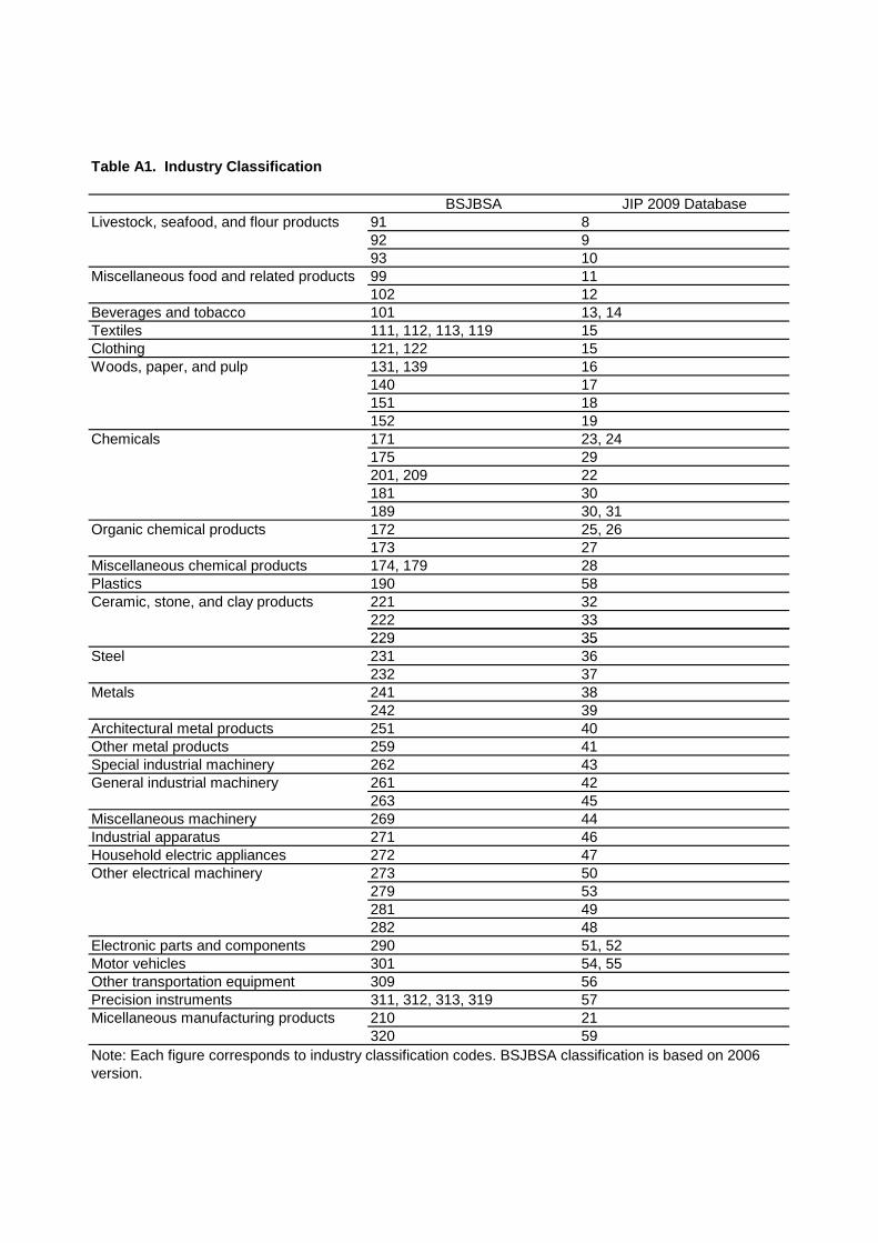
Table A1. Industry Classification

BSJBSA JIP 2009 DatabaseLivestock, seafood, and flour products 91 8

92 993 10

Miscellaneous food and related products 99 11102 12

Beverages and tobacco 101 13, 14Textiles 111, 112, 113, 119 15Clothing 121, 122 15Woods, paper, and pulp 131, 139 16

140 17151 18152 19

Chemicals 171 23, 24175 29201, 209 22181 30189 30, 31

Organic chemical products 172 25, 26173 27

Miscellaneous chemical products 174, 179 28Plastics 190 58Ceramic, stone, and clay products 221 32

222 33229229 3535

Steel 231 36232 37

Metals 241 38242 39

Architectural metal products 251 40Other metal products 259 41Special industrial machinery 262 43General industrial machinery 261 42

263 45Miscellaneous machinery 269 44Industrial apparatus 271 46Household electric appliances 272 47Other electrical machinery 273 50

279 53281 49282 48

Electronic parts and components 290 51, 52Motor vehicles 301 54, 55Other transportation equipment 309 56Precision instruments 311, 312, 313, 319 57Micellaneous manufacturing products 210 21

320 59Note: Each figure corresponds to industry classification codes. BSJBSA classification is based on 2006version.

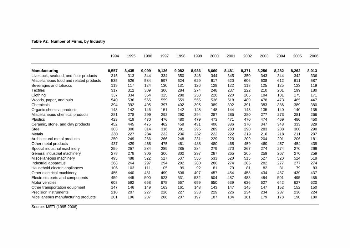
Table A2. Number of Firms, by Industry

1994 1995 1996 1997 1998 1999 2000 2001 2002 2003 2004 2005 2006

Manufacturing 8,557 8,435 9,099 9,136 9,082 8,936 8,660 8,481 8,371 8,256 8,282 8,262 8,013Livestock, seafood, and flour products 315 313 344 334 350 346 344 345 350 343 344 342 336Miscellaneous food and related products 535 526 584 597 624 629 617 620 606 608 612 611 587Beverages and tobacco 119 117 124 130 131 126 128 122 118 125 125 123 119Textiles 317 312 309 306 284 274 248 237 222 210 201 199 180Clothing 337 334 354 325 288 258 228 220 205 184 181 175 171Woods, paper, and pulp 540 536 565 559 559 555 536 518 489 478 473 465 447Chemicals 394 392 405 397 402 395 389 392 391 383 386 389 380Organic chemical products 143 142 146 151 142 148 148 144 143 135 140 140 135Miscellaneous chemical products 281 278 299 292 290 294 287 285 280 277 273 281 266Plastics 423 419 470 476 480 479 473 471 470 474 469 480 450Ceramic, stone, and clay products 452 445 475 462 458 431 406 386 370 347 348 333 329Steel 303 300 314 316 301 295 289 283 290 283 288 300 290MetalsMetals 230230 227227 234234 232232 230230 232232 222222 222222 219 216 218 211 207219 216 218 211 207Architectural metal products 250 249 266 266 248 231 229 223 209 204 201 206 181Other metal products 437 429 458 475 481 488 480 468 459 460 457 454 439Special industrial machinery 259 257 284 289 285 284 279 270 267 274 274 270 266General industrial machinery 278 278 306 306 302 297 287 265 265 259 267 270 259Miscellaneous machinery 495 488 522 527 537 536 533 520 515 527 520 524 518Industrial apparatus 268 264 297 294 292 280 286 274 285 282 277 277 274Household electric appliances 106 103 111 105 99 92 81 79 81 82 81 79 83Other electrical machinery 455 440 481 499 506 497 457 454 453 434 437 439 437Electronic parts and components 459 445 500 523 531 532 504 487 488 484 501 495 485Motor vehicles 603 592 668 678 667 659 650 639 636 627 642 627 620Other transportation equipment 147 146 149 163 161 148 143 147 145 147 152 152 150Precision instruments 210 207 227 226 227 233 229 226 234 234 237 230 224Micellaneous manufacturing products 201 196 207 208 207 197 187 184 181 179 178 190 180

Source: METI (1995-2006)