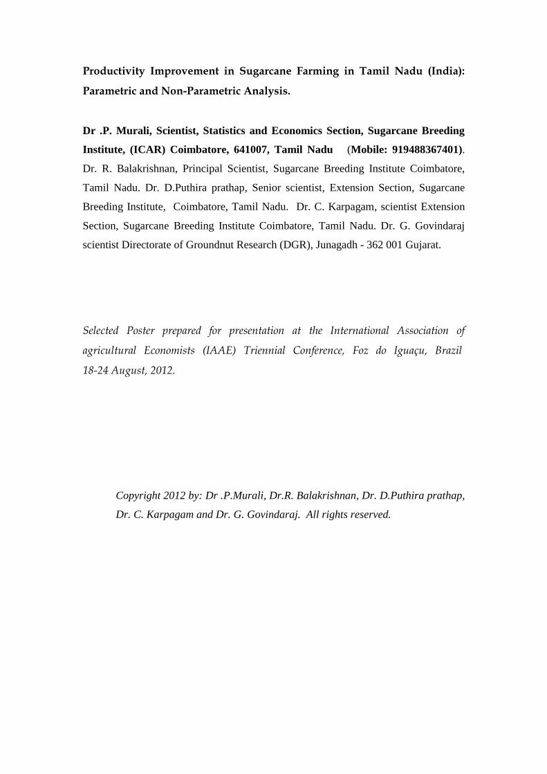
Productivity Improvement in Sugarcane Farming in Tamil Nadu (India):

Parametric and Non-Parametric Analysis.

Dr .P. Murali, Scientist, Statistics and Economics Section, Sugarcane Breeding

Institute, (ICAR) Coimbatore, 641007, Tamil Nadu (Mobile: 919488367401).

Dr. R. Balakrishnan, Principal Scientist, Sugarcane Breeding Institute Coimbatore,

Tamil Nadu. Dr. D.Puthira prathap, Senior scientist, Extension Section, Sugarcane

Breeding Institute, Coimbatore, Tamil Nadu. Dr. C. Karpagam, scientist Extension

Section, Sugarcane Breeding Institute Coimbatore, Tamil Nadu. Dr. G. Govindaraj

scientist Directorate of Groundnut Research (DGR), Junagadh - 362 001 Gujarat.

Selected Poster prepared for presentation at the International Association of

agricultural Economists (IAAE) Triennial Conference, Foz do Iguaçu, Brazil

18-24 August, 2012.

Copyright 2012 by: Dr .P.Murali, Dr.R. Balakrishnan, Dr. D.Puthira prathap,

Dr. C. Karpagam and Dr. G. Govindaraj. All rights reserved.

1

PRODUCTIVITY IMPROVEMENT IN SUGARCANE FARMING IN TAMIL

NADU (INDIA): PARAMETRIC AND NON-PARAMETRIC ANALYSIS

ABSTRACT

Sugarcane productivity is cyclical in India and Tamil Nadu. The post-Green

Revolution phase is characterized by high input-use and decelerating total factor

productivity growth. Sugarcane productivity attained during the 1980s has not been

sustained during the1990s and early 21st

century and has posed a challenge for the

researchers to shift production function upward by improving the technology index.

Examination of issues related to the sugarcane productivity, particularly with

reference to Tamil Nadu state which has highest yield in India. Data envelopment

analysis (DEA) and stochastic frontier analysis (SFA) used to assess productivity

growth of sugarcane farming. The results show consistency between the approaches

and there are potentials for efficiency improvements. Second, there has been a

productivity improvement in the sector, in the interval 0.7–15% in the periods studied

and technical change had the greatest impact on productivity. The average TFP in

after introducing variety Co 86032 was larger than that of pre- introduction of this

variety. In both periods, productivity growth is sustained through technological

progress. In general, policy-makers should try not to be indifferent with respect to the

approach used for productivity measurement as these may give different results.

Key words: Sugarcane, TFP, Malmquist Index, variety Co 86032

2

INTRODUCTION

Sugarcane is the second most important industrial crop in the country is grown

about 5 million hectares. The growth of sugarcane agriculture in the country had been

consistent during the past seven decades. There was increase in area, production,

productivity and sugar recovery. During the period from 1930-31 to 2010-11, the area

under sugarcane had gone up from 1.18 million ha to 5.0 million ha, productivity from

31 tonnes to 70 tonnes per hectare and total cane produced from 37 million tonnes to

340 million tonnes. Current sugar production in the country is about 24.5 million

tonnes (Co-operative sugar 2011).

Among the sugarcane growing states in India, Tamil Nadu ranks third in area

( 0.37 M.ha) and production ( 3.5 Million tonnes) and first in productivity ( 105 t/ha)

and sugarcane productivity is 40% higher than the national productivity (69.5 t/ha).

The area and production of sugarcane at Tamil Nadu is comparable as equal as

Australia and USA.

One of the notable characteristics of the sugarcane agriculture in the country is

its inherent instability. The cane productivity in the state is dependent on rainfall and

drought spells appearing in regular intervals leading to wide fluctuations in cane

productivity. Rising yields also contributed to the growth in sugarcane production.

Yields rose by more than 30% from an average of 75 tonnes/ha in the early-sixties to

more than 105 tonnes/ha in the mid-nineties. Following rapid increases in productivity

in the seventies and early-eighties, the rate of growth slackened in the latter part of the

nineties. The extension of cane area to marginal lands and the use of varieties

susceptible to disease were partly responsible for the slower growth. However, an

average sugarcane yield varies region to region in the state which greatly affects the

cost of cane production in the state.

3

To improve the productivity and efficiency of the sugarcane production

system, new varieties and technologies were introduced in the state to shift the

productivity horizon. Never the less, the yield scenario did not change much and

become cyclical and uneven up to 1999, however, new noble variety (Co 86032 )was

introduced in the state, then the yield was increased significantly. Hence, to identify

the different factors responsible for the productivity growth, this study was

undertaken with panel data to estimate technical change, efficiency change and total

factor productivity of sugarcane production system of the state.

Total Factor Productivity (TFP) of Sugarcane

Productivity growth in agriculture is both a necessary and sufficient condition

for its development and has remained a serious concern for intense research over the

last five decades. Solow (1957) was the first to propose a growth accounting

framework, which attributes the growth in TFP to that part of growth in output, which

cannot be explained by growth in factor inputs like land, and capital. Development

economists and agricultural economists have computed productivity and have

examined productivity growth over time and differences among countries and regions.

Productivity growth is essential to meet the food demands arising out of steady

population and economic growth.

TFP is an important measure to evaluate the performance of any production

system and sustainability of a growth process. However, a number of complex

conceptual issues are not adequately captured by an analysis of the kind described

earlier. First, for example, agricultural research has contributed to breaking the

seasonality in crop production. Second, a great deal of stability has been introduced in

crop production by providing farmers with varieties that tolerate or resist adverse

environmental conditions. Finally, high sugar recovery improvements have added to

4

the value of production as in the case of sugarcane production. All of these and many

other contributions have been subsumed under a residual TFP measure. It would be

worthwhile to identify these influences explicitly, which would lead to a more

realistic assessment of the productivity of sugarcane production system.

The productivity in each district is conditioned by various micro and macro

environmental and biotic factors besides socio-economic aspects. There is a wide gap

in productivity between the fertile and the marginal soil and climate regions of the

state, the former averaging about 125 t/ha and the latter 90 t/ha. Wide gap exists

between the potential yield and the yield levels achieved at present in all the

districts/regions without exception. Bridging of the yield gap should be the primary

focus for attaining the projected targets for the future.

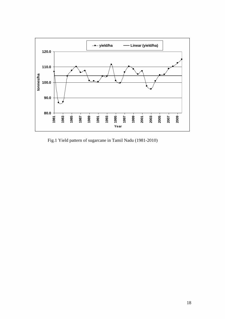
To provide an historical perspective on sugarcane productivity, figure 1

depicts productivity over the last three decades (1981–2010). Before introduction

noble variety (Co86032), productivity has been sluggish, with year to-year

fluctuations. Since 1979/1980 production season, there seems to be some

improvement in the productivity of sugarcane in this period (1999-2010). Largest

improvement can be observed in the recent past.

While much evidence has been provided attesting the productive performance

of the agricultural sector in India and factors influencing it (Kumbakar and Lovell,

2000: Kumar et al., 2003, 2006 and 2008) there is little evidence on sugarcane crop –

specific and sub – regional productive performance. An assessment of crop – specific

efficiency and productivity analysis should be of more interest to policy-makers

implementing liberalization policy than overall aggregates.

The rationale is twofold; (a) An insight can be gained on the potential for

resource savings and productivity improvements of sugarcane crops and, (b) the

5

producers can learn from the front-runners how best to utilize their resources

efficiently. Inter alia, issues of interest in this study are: (a) is there any potential for

improving the efficiency of sugarcane producers in Tamil Nadu? If so, what are the

magnitudes? (b) Has there been any productivity progress in Tamil Nadu cane

production since 1981? The choice of 1981 as reference point is highest yield

recorded since post green revolution period in the state. (a) and (b) irrespective of the

methodology applied? While questions (a) and (b) are interesting to the extent that the

much needed insight on the performance the sector is gained, question (c) provides

evidence on the consistency of frontier techniques within two different and most

commonly used approaches.

This is of considerable interest for policy purpose. If methods do not give

results that are similar or highly correlated to each other, the policy may be fragile and

depends on which frontier approach is employed. While the vast majority of empirical

studies on productivity growth in the agricultural sector mostly have utilized only one

method to estimate their efficiencies, this study focuses on two methodological

approaches for measuring efficiency as follows:

(1) The construction of a nonparametric piecewise linear frontier using linear

programming method known as data envelopment analysis (DEA) (Charnes et al.,

1978);

(2) The construction of a parametric production function using stochastic frontier

analysis (SFA) (Aigner et. al 1977; Meeusen and van de Broeck, 1977; Battese and

Coelli, 1992, Coelli, 1996).

The data

The farm-level data on sugarcane yield and the use of inputs and their prices

from year 1981 to 2010 collected under the "Comprehensive scheme for the study of

6

cost of cultivation of principal crops," Directorate of Economics and Statistics (DES),

Government of India (GOI), were used in the analysis of TFP. The out put prices were

collected from various issues co-operative sugar journal of 1980 to 2011. The missing

year data on inputs and their prices were collected using interpolations based on

trends of the available data. The time-series data on area, yield, production, irrigated

and high-yielding variety (HYV) area for the sugarcane were taken from the various

published reports of the DES (GOI). The share of the hills region in sugarcane

production was marginal and was therefore not included in the analysis.

The rest of this paper is organized as follows: The theoretical foundation for

the stochastic and non-stochastic measurement of the TFP in section 2. Section 3, the

data used is described and the parameter estimates are reported to infer which factors

explain the growth of output. A final section concludes.

II. Methodology

This study utilizes two methodological approaches for measuring efficiency

namely: data envelopment analysis (DEA) (Charnes et al. 1978) and production

function using stochastic frontier analysis (SFA) (Coelli, 1996). For measuring

productivity growth, both methods and their extensions to Malmquist index approach

are used throughout the study. Each of the methods and their subsequent Malmquist

indices is briefly described as follows:

2/1

1

1

00

11),(

)1,1(*

),(

)1,1(),,,(

tt

t

o

tt

t

tt

t

o

tt

t

ttttoyxd

yxd

yxd

YxdyxyxM -------------- (1)

Where td0 ),( tt yx is the output distance for year t, which is defined as the ratio

of observed output to the maximum output, y producible with given technology and

7

input vectors, x (Shapard, 1970). The superscript is the value of the output distance

evaluated input-output of year t+1 using technology of year t.

Equation (1) can be decomposed into the following two components namely

efficiency change index which measures the output –oriented shift in technology

between two periods and the technical change between period t+1 and t. If the

technical change is greater (or less) than one, then technological progress (or regress)

exists.

Symbolically,

EFFCHI = ),(

),(11

1

tt

t

o

tt

t

o

yxd

Yxd

----------------- (2)

and

TECHCHI =

2/1

1

11

1

0

11

110

),(

),(*

),(

),(

tt

t

o

tt

t

tt

t

o

tt

t

yxd

yxd

yxd

Yxd ---------(3)

There exist several methods of estimating the distance functions which makes

up the Malmquist TFP index. The most popular and widely adopted in recent time has

been the DEA like linear programming (LP) methods suggested by Fare et. al (1994)

and its parametric equivalent – stochastic frontier method adopted in this study.

Stochastic Frontier Method

The stochastic production function for panel data can be written as

In ),,,(( itititit uvtxfy ---------------------------------- (4)

I = 1, 2, ………N and t = 1, 2, ………T (Battese and Coelli 1992)

Where yit is production of the ith firm in year t, α is the vector of parameters to

be estimated. The vit are the error component and are assumed to follow a normal

distribution N ( itit u),,0 2 are non negative random variable associated with technical

8

inefficiency in production which are assumed to arise from a normal distribution with

mean u and variance 2

which is truncated at zero. F(.) is a suitable form (e.g

translog), t is a time trend representing the technical change.

In this parametric case, according to Coelli et. Al (1998), the technical

efficiency (TE) are obtained as

TEit = E(exp) (-uit)/vit – uit) ----------------------------- (5)

This can be used to compute the efficiency change component by observing that

TEit = td0 ),( itit yx and 1,tTEi

td0 t+1 ),( 1,1, titi Yx the efficiency change (EC) is

EC = TEit / TEi,t+1 ---------------------------------------------------------(6)

An index of technological change between the two adjacent periods t and t+1

for the ith region can be directly calculated from the estimated parameters of the

stochastic production frontier by simply evaluating the partial derivatives of the

production function with respects to time at itx and 1, tix Following Coelli et al (1998),

the technical change (TC) index is

21

,,(1

1

,1,(1

/

itit

f

txfx

f

txfTCit

------------------------------ (7)

The TFP index can be obtained by simply multiplying the technical change

and the technological change i.e

TFPit = ECit *TCit ----------------------------------------------------------------------------------------------- (8)

This is equivalent to the decomposition of the Malmquist suggested by Fare et al

(1994).

Empirical Specification

This study utilized data on output and inputs of sugarcane of the Tamil Nadu

to construct indices of TFP using the two methods described by equations 1 – 8. The

sample data comprise annual measures of the output of each crop and 6 direct inputs

9

(land area, seed, fertilizer, labour, machine labour and irrigation). For the purposes of

the present study, several functional forms were fitted beginning with Cobb-Douglas

technology. The underlying stochastic production frontier function upon which the

results and discussion of this study are based is approximated by the generalized

Cobb-Douglas form (Fan 1991). The function may also be viewed as a translog

specification without cross terms, i.e. a strongly separable-inputs translog production

frontier function of the sugarcane is specification as:

In yit = αo+αh In Hit + αs, In Sit + αf In Fit + αl In Lit + In Kit + In Iit + αtt+2

1 αnt2+αht

(In Hit)t+αst (In Sit)+αft (In Fit) t+αit (In Lit) t+αkt(In Kit)t+ait (InIit)t+vit-uit ----------------- (9)

Yit is the output of crop i in the year

Hit is the hectares of land cultivated sugarcane each year

Sit is the quantity of seed planted in ‘tonnes

Fit is the quantity of fertilizer used in ‘kgs

Lit is amount of labour used in mandays

Kit is the amount of machine labour used in man days

Iit is the proportion of each crop land area under irrigation

In is the natural log

αi s are unknown parameters to be estimated

vit s are iidN (0, σ,) random errors and are assumed to be independently distributed of

the uit s which are non negative random variables associated with TE inefficiency.

Outputs:

This is the Quantity of sugarcane production in ’000 kgs.

Inputs Fertilizer: Fertilizer use is proxyed as the total fertilizer use in kgs.

Labour: This is measured as the amount of labour in cane production proxyed as the

10

economically active agricultural labor force per unit of area.

Machine labour: it refers to the amount of machine and skilled machine operator

used in cane production.

Land: Expressed in ‘000 ha, it is measured as land area under cane cultivation.

Seed: expressed in ‘000 metric tonnes, it covers quantity of sugarcane seed (setts)

planted/ha.

Irrigation: This is the proportion of rice land area that is irrigated.

III. EMPIRICAL RESULTS AND ANALYSIS

The results of the analysis are in two steps. First we outline the results based

on the SFA and DEA approaches. Then we present the efficiency and technical

change results of both methods, followed by the Total Factor Productivity Analysis.

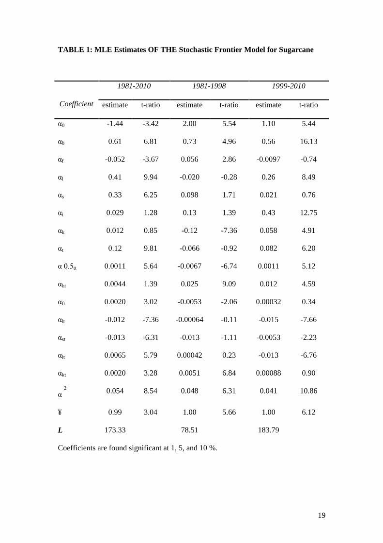
The Results of the Stochastic Frontier Model

Parametric productivity measures are based on the estimated parameters of the

stochastic frontier function (9), and so a brief discussion of these estimates and their

statistical properties precedes our comparative analysis of productivity indices. The

estimated parameter of the stochastic quasi translog production frontier function is

estimated using FRONTIER 4.1 software (Coelli, 1996). The parameter estimates of

the model for the whole period (1981-2010), pre-introduction of variety Co86032

period (1981-1998) and introduction of variety Co86032 period (1999-2010) were

presented in Table 1. The variance parameters, α 2

and ¥ are significantly different

from zero. This provides statistical confirmation of the presumption that there are

differences in technical efficiency among farmers. The mode of the truncated normal

distribution µ, is significantly different from zero, providing statistical evidence that

the distribution of the random variable µ, has a non-zero mean and is truncated below

11

zero. Thus the stochastic frontier production function is empirically justified. Further,

logarithm of the likelihood function indicates a satisfactory fit for the generalized

Cobb Douglas specification. The statistical significance of all of the parameters α 2

and L reinforces the view that technical efficiency affects productivity.

The Maximum Likelihood Estimates (MLE) results indicate that twelve out of

fifteen variables are found to be statistically significant. Apart from fertilizer, the

coefficients of all the variables have the expected positive signs over the entire

analysis period. The negative coefficient of fertilizer over the entire analysis period

suggests operation in stage III of the production function where there is considerable

congestion in the use of fertilizer. Such congestion might be due to late availability of

fertilizer to farmers in the state. Over the analysis period the coefficient of both labour

and capital are positive and significant. The coefficient on the time trend indicates

positive technological progress in sugarcane production between 1981 and 2010. The

frontier is shifting upwards at annual rate of 8 %. The technological progress actually

takes place after introduction of variety Co86032 indicated technological decline in

pre-introduction of variety Co86032 in the state.

IV. Total factor productivity (TFP) and its decomposition

Malmquist productivity indices: SFA

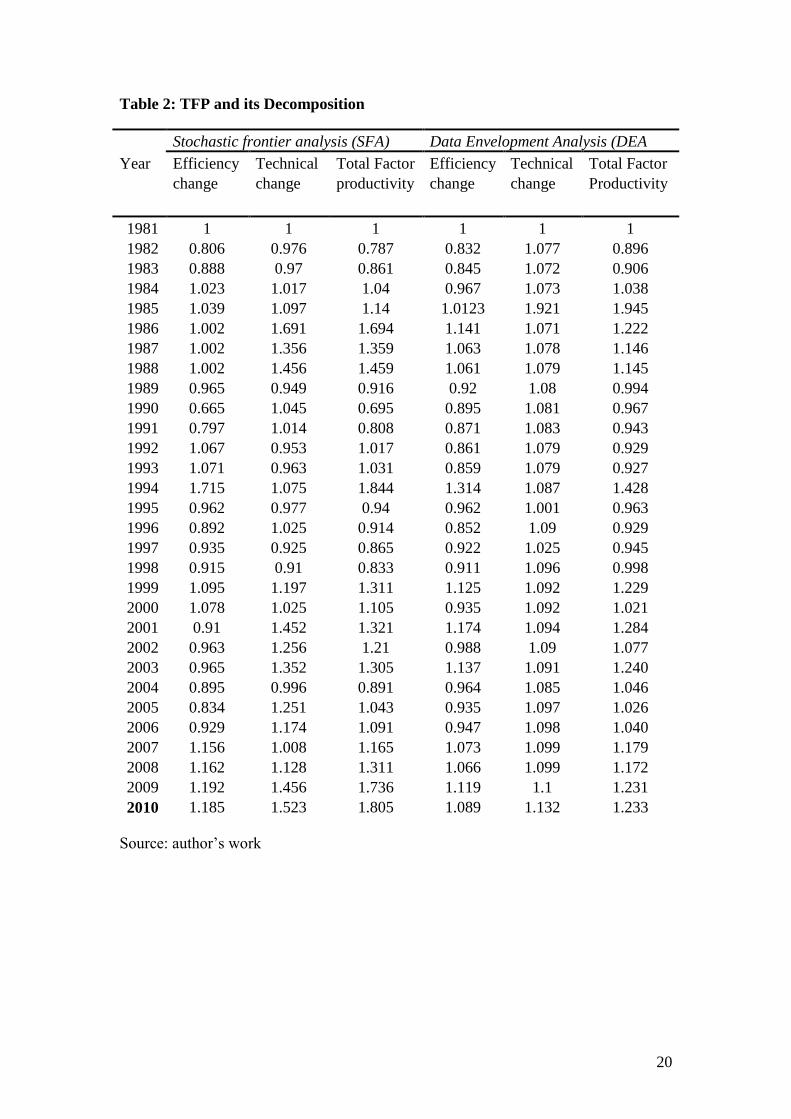
The summary description of the average annual TFP obtained from using the

stochastic frontier analysis and its decomposition into efficiency and technical

changes over the entire period for each country are presented in Table 2. The

evolution is made clearer in figure 2. It should be recalled that if the value of the

Malmquist index or any of its components is less than one, it implies regress between

two adjacent periods, whereas values greater than 1 imply progress or improvement.

12

The values of the indices capture productivity relative to the best performers. In this

study, the Malmquist indices measure year to year changes in productivity. The

evolution in Figure 2 indicates that differences exist among the years.

A comparison of the productivity in the pre-introduction of variety Co86032

period with after introduction of variety Co86032 period (Table 2) shown that more

technological progress and hence more improvement in productivity was recorded

after introduction of variety Co86032 than pre-introduction of variety Co86032

period. The mean technical change after introduction of variety Co86032 and pre

introduction of variety Co86032 periods were 1.234 and 1.140 respectively. The

annual TFP growth over the whole period is 7.6%. The improvement was more due to

technological progress rather than improvement in efficiency. A major contributor to

sugarcane TFP growth in the recent decades has been the technical change. The TFP

changes indicate more progress after introduction of variety Co86032 than pre-

introduction of variety Co86032. Two things could be responsible for this

phenomenon. First, the impressive research of sugarcane breeding institute (SBI) and

extension department of the sugar factories which led to adoption of improved Co

86032 variety of sugarcane at Tamil Nadu. The second is the competitive State

Advised Price (SAP) for sugarcane which tend to boost farmers’ income in the recent

time period in the state.

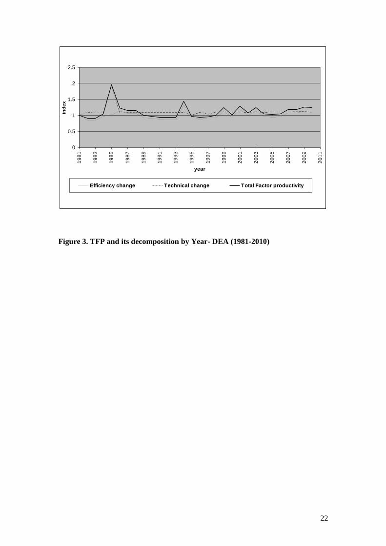
DEA Result

The same sample data were used to calculate the set of indices using DEA-like

method described in equations 1 to 3. The calculations were done using a DEAP

version 2.1 Computer programme and the evolution is shown in Figure 3. The overall

TFP growth rate was 4.3% and it is driven mainly by technical change as was the case

with the stochastic approach. In general however, the two approaches agree that over

13

the analysis period, there have been a productivity progress in the sugarcane

production system of Tamil Nadu. Like the SFA approach, the DEA approach show

on the average that efficiency change indices are smaller than the technical change

components. Also, it can be observed that the TFP of SFA are higher than DEA’s

perhaps because the efficiency scores of SFA tends to be higher than DEA’s. Quite

similar conclusion was reached by Kwon and Lee 2004 when considering the TFP of

Korean rice using both DEA and SFA methods. The finding is however contrary to

Odeck 2007 who discovered that the DEA’s efficiency scores and TFPs tend to be

higher than SFA in Norwegian grain farming.

Over the entire analysis period, the efficiency change is about 0.994 which is

by far lower than 1.048 obtained in case of stochastic approach. However, an even

greater difference is observed in the technical change component. Though both

methods indicate TFP progress, the SFA indicates more productivity progress than the

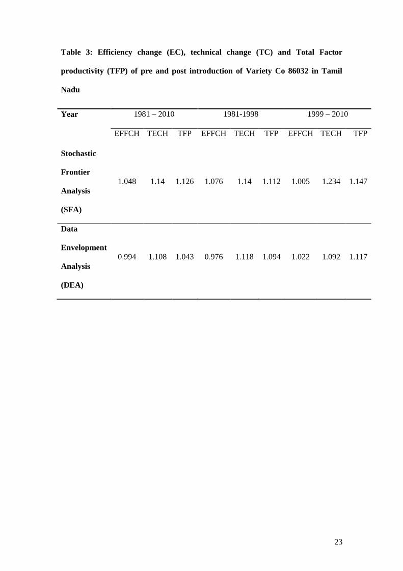
DEA method over the analysis period. Table 3 shows a summary description of the

average performance of the entire time period of 1981 – 2010; pre-introduction of

Co86032 (1981-1998) and after introduction of Co86032 (1999 – 2010). Taking a

look at the result, the entire period (1981 – 2010) productivity increased on the

average 8%. However TFP decline on the average in pre- introduction of Co86032

period whereas the average change in the total factor productivity index was 4.5%.

The growth in was due mainly to innovation rather than improvement in efficiency.

The result of this study differ significantly from few examples of rice – specific TFP

studies such as Cassman and Pingali (1995) and Pardey et al. (1992). While they

discover decline in rice TFP in Asia, the result of this study indicates increase.

Another major difference is that the major source of rice productivity growth in Asia

is efficiency change while in sugarcane it is due mainly to technical change. The use

14

of inputs efficiently in Asia contributes more to TFP growth than net gains from

technological change. Hence, the sugarcane policy content of Tamil Nadu could be re-

defined to accommodate productivity increasing policies inherent in ASEAN green

revolution.

V. CONCLUSION AND POLICY RECOMMENDATION

The present research applied non-parametric and parametric models to a sample of

panel data of sugarcane production for the period of 1981–2010. The productivity

growth was estimated using the Malmquist index obtained through both parametric

and non-parametric approaches. The productivity measures are decomposed into two

sources of growth namely efficiency change and technical change. The results show

evidence of phenomenal growth in the TFP after introduction of Co86032. In both

periods, productivity is sustained through technological progress. Several inferences

may now be drawn from the comparative analysis of DEA and SFA efficiency and

productivity models examined. First, the non-parametric results tend to fluctuate

widely. This is clearly the consequence of the assumption on the stochastic

component, something which may be intensified for agricultural data. The second is

that inefficiency and productivity growth exists over the decadal period. The

magnitude of inefficiency and the extent of productivity growth that has taken place

vary between the approaches applied. Third, examining the components relating to the

shift in the frontier (TC) and efficiency change (EC), technical change turned out to

be a more important source of growth in both parametric and non-parametric models.

A promising finding there upon is that the two approaches applied are, on average,

in conformity to each other although the magnitudes are different. In terms of

efficiency measurements, the differences between the methodologies are very

sensitive on levels of segmentations. In this respect, the somehow conform to

15

previous findings in the literature e.g., Wadud and White (2000). In terms of

productivity measurement, even though both approaches track total productivity

similarly, they do not map each well at the decomposition level. The deviations

between DEA and SFA could have been anticipated because the SFA incorporates

stochastic factor while DEA does not. The differences between the techniques applied

here suggests that policy-makers as well as researchers should not be indifferent as to

the choice of technique for assessing efficiency and productivity, at least with respect

to the magnitudes of potential for efficiency improvements and productivity growth.

Finally, studies have not been able to detect why and how the different approaches

are so different with respect to the decomposed productivity measures. In this respect

necessary caution should be observed against widespread application of either SFA or

DEA until such time that the field of efficiency and productivity measurement

understand how and why these approaches portray efficiency and productivity the

way they do. To this end, there is a need for continuous research in understanding the

differences observed, which in this study concerns the magnitudes rather than

conflicts. Further limitation of the study is that the data used as shown in the yield

curves tend to fluctuate considerably. This mean that yield of sugarcane was

influenced by climate and soil parameters. Given the caution in interpreting the

results, the following policy recommendations are suggested from the findings:

1. The government of Tamil Nadu should invest more in functional agricultural

extension services to enhance efficient use of available productivity increasing

inputs.

2. Given differences in the contribution of efficiency change and technological

progress to the TFP of the sugarcane, the research institute focus to develop

input responsive sugarcane varieties to improve efficiency of the crop.

16

REFERENCES

Aigner, D.J., Lovell, C.A.K. and Schmidt, P. 1977. ‘Formulation and estimation of

stochastic frontier production function models’, Journal of Econometrics, vol.

6, pp. 21–37.

Battese, G.E. and Coelli, T.J. 1992. ‘Production frontier functions, technical

efficiencies and panel data: with application to paddy farmers in India’,

Journal of Productivity Analysis, vol. 3, pp. 153–169.

Cassman, K.G., and P.L. Pingali. 1995. Extrapolating trends from long term

experiments to farmers fields: the case of irrigated rice systems in Asia. In: V.

Barnett, Caves D.W., L.R. Christensen and W.E. Diewert. 1982. The

Economic Theory of Index Numbers and Measurement of Input, Output and

Productivity. -Econometrica, 50, 1393-1414.

Charnes, A., Cooper, W.W. and Rhodes, E. 1978. ‘Measuring efficiency of decision

making units’, European Journal of Operational Research, vol. 2, pp. 429–

444.

Coelli, T., A. 1996. Guide to DEAP, Version 2.1: A Data Envelopment Analysis

(Computer) Program. Center for Efficiency and Productivity Analysis.

University of New England. Working paper, 96/08.

Coelli, E. G., Rao, D. S. P. and Battese, G. E. 1998. An Introduction to Efficiency and

Productivity Analysis, Kluwer Academic Publishers,

Boston/Dordretch/London.

Cooperative sugar 2011. National Federation of Cooperative Sugar Factories Ltd.

New delhi.

Fan, S. 1991. Effects of technological change and institutional reform on production

growth in Chinese agriculture. American Journal of Agricultural Economics

73(2): 266–275.

Fare, R;S, Grosskopf, M. Norris and Z. Zhang 1994. Productivity growth, technical

progress and efficiency change in industrialized countries. American

Economic Review 84: 66 – 83.

Kumar, Praduman and Mittal, Surabhi 2003. Productivityand supply of food grains in

India, In: Towards a Food Secure India: Issues & Policies, Eds: S. Mahendra

Dev,K.P. Kannan and Nira Ramachandran, Manohar Publishers and

Distributers. pp. 33-58.

17

Kumar, Praduman and Mittal, Surabhi 2006. Agriculturalproductivity trend in India:

Sustainability Issues. Agricultural Economics Research Review,

19(Conference No.): 71-88.

Kumar, Praduman, Mittal, Surabhi and Hossain, Mahabub 2008. Agricultural growth

accounting and total factorproductivity in South Asia: A review and

policyimplications, Agricultural Economics Research Review,21(2): 145-172.

Kumbhakar, S. C. and C. Lovell 2000 . Stochastic Frontier Analysis, Cambridge

University Press, Cambridge.

Kwon, O. S. and H. Lee 2004. Productivity mprovement in Korean rice farming:

parametric and non-parametric analysis The Australian Journal of Agricultural

and Resource Economics , 48:2, pp. 323–346.

Montpellier Palavas Meeusen, W. and van de Broeck, J. 1977. Efficiency estimation

from Cobb-Douglas production functions with composite error, International

Economic Review,18, 435–44. Malmquist, S. 1953. Index Numbers and

Indifference Curves. Trabajos de Estatistica, 4, 1, 209.

Odeck, James 2007. 'Measuring technical efficiency and productivity growth: a

comparison of SFA and DEA on Norwegian grain production data', Applied

Economics, 39:20, 2617 – 2630.

Pardey, P. G; J. Roseboom and B. J. Craig 1992. A yardstick for international

comparisons: An application to national agricultural research expenditures,

Economic Development and Cultural Change 40(2); 333-349.

Shephard R. W. 1970. Theory of cost and production functions. Princeton university

press, Princeton.

Solow, R.M., (1957) Technical change and aggregate production function, Reviewof

Economics and Statistics, 39(3): 312-320.

Wadud, A. and White, B. 2000 Farm household efficiency in Bangladesh: a

comparison of stochastic frontier and DEA methods, Applied Economics, 32,

1665–73. World Bank (2007). World Agricultural Development Indicators.

Washington D.C.

18

80.0

90.0

100.0

110.0

120.01981

1983

1985

1987

1989

1991

1993

1995

1997

1999

2001

2003

2005

2007

2009

Year

ton

ne

s/h

a

yield/ha Linear (yield/ha)

Fig.1 Yield pattern of sugarcane in Tamil Nadu (1981-2010)

19

TABLE 1: MLE Estimates OF THE Stochastic Frontier Model for Sugarcane

Coefficient

1981-2010 1981-1998 1999-2010

estimate t-ratio estimate t-ratio estimate t-ratio

α0 -1.44 -3.42 2.00 5.54 1.10 5.44

αh 0.61 6.81 0.73 4.96 0.56 16.13

αf -0.052 -3.67 0.056 2.86 -0.0097 -0.74

αl 0.41 9.94 -0.020 -0.28 0.26 8.49

αs 0.33 6.25 0.098 1.71 0.021 0.76

αi 0.029 1.28 0.13 1.39 0.43 12.75

αk 0.012 0.85 -0.12 -7.36 0.058 4.91

αt 0.12 9.81 -0.066 -0.92 0.082 6.20

α 0.5tt 0.0011 5.64 -0.0067 -6.74 0.0011 5.12

αht 0.0044 1.39 0.025 9.09 0.012 4.59

αft 0.0020 3.02 -0.0053 -2.06 0.00032 0.34

αlt -0.012 -7.36 -0.00064 -0.11 -0.015 -7.66

αst -0.013 -6.31 -0.013 -1.11 -0.0053 -2.23

αit 0.0065 5.79 0.00042 0.23 -0.013 -6.76

αkt 0.0020 3.28 0.0051 6.84 0.00088 0.90

α 2

0.054 8.54 0.048 6.31 0.041 10.86

¥ 0.99 3.04 1.00 5.66 1.00 6.12

L 173.33 78.51 183.79

Coefficients are found significant at 1, 5, and 10 %.

20

Table 2: TFP and its Decomposition

Stochastic frontier analysis (SFA) Data Envelopment Analysis (DEA

Year Efficiency

change

Technical

change

Total Factor

productivity

Efficiency

change

Technical

change

Total Factor

Productivity

1981 1 1 1 1 1 1

1982 0.806 0.976 0.787 0.832 1.077 0.896

1983 0.888 0.97 0.861 0.845 1.072 0.906

1984 1.023 1.017 1.04 0.967 1.073 1.038

1985 1.039 1.097 1.14 1.0123 1.921 1.945

1986 1.002 1.691 1.694 1.141 1.071 1.222

1987 1.002 1.356 1.359 1.063 1.078 1.146

1988 1.002 1.456 1.459 1.061 1.079 1.145

1989 0.965 0.949 0.916 0.92 1.08 0.994

1990 0.665 1.045 0.695 0.895 1.081 0.967

1991 0.797 1.014 0.808 0.871 1.083 0.943

1992 1.067 0.953 1.017 0.861 1.079 0.929

1993 1.071 0.963 1.031 0.859 1.079 0.927

1994 1.715 1.075 1.844 1.314 1.087 1.428

1995 0.962 0.977 0.94 0.962 1.001 0.963

1996 0.892 1.025 0.914 0.852 1.09 0.929

1997 0.935 0.925 0.865 0.922 1.025 0.945

1998 0.915 0.91 0.833 0.911 1.096 0.998

1999 1.095 1.197 1.311 1.125 1.092 1.229

2000 1.078 1.025 1.105 0.935 1.092 1.021

2001 0.91 1.452 1.321 1.174 1.094 1.284

2002 0.963 1.256 1.21 0.988 1.09 1.077

2003 0.965 1.352 1.305 1.137 1.091 1.240

2004 0.895 0.996 0.891 0.964 1.085 1.046

2005 0.834 1.251 1.043 0.935 1.097 1.026

2006 0.929 1.174 1.091 0.947 1.098 1.040

2007 1.156 1.008 1.165 1.073 1.099 1.179

2008 1.162 1.128 1.311 1.066 1.099 1.172

2009 1.192 1.456 1.736 1.119 1.1 1.231

2010 1.185 1.523 1.805 1.089 1.132 1.233

Source: author’s work

21

0

0.5

1

1.5

2

19

80

19

82

19

84

19

86

19

88

19

90

19

92

19

94

19

96

19

98

20

00

20

02

20

04

20

06

20

08

20

10

Year

Ind

ex

Efficiency change Technical change Total Factor productivity

Figure 2. TFP and its decomposition by Year- SFA (1981-2010)

22

0

0.5

1

1.5

2

2.5

19

81

19

83

19

85

19

87

19

89

19

91

19

93

19

95

19

97

19

99

20

01

20

03

20

05

20

07

20

09

20

11

year

ind

ex

Efficiency change Technical change Total Factor productivity

Figure 3. TFP and its decomposition by Year- DEA (1981-2010)

23

Table 3: Efficiency change (EC), technical change (TC) and Total Factor

productivity (TFP) of pre and post introduction of Variety Co 86032 in Tamil

Nadu

Year 1981 – 2010 1981-1998 1999 – 2010

EFFCH TECH TFP EFFCH TECH TFP EFFCH TECH TFP

Stochastic

Frontier

Analysis

(SFA)

1.048 1.14 1.126 1.076 1.14 1.112 1.005 1.234 1.147

Data

Envelopment

Analysis

(DEA)

0.994 1.108 1.043 0.976 1.118 1.094 1.022 1.092 1.117