Full Terms & Conditions of access and use can be found athttp://www.tandfonline.com/action/journalInformation?journalCode=raec20

Download by: [49.174.5.30] Date: 09 February 2016, At: 02:19

Applied Economics

ISSN: 0003-6846 (Print) 1466-4283 (Online) Journal homepage: http://www.tandfonline.com/loi/raec20

Productivity growth and stock returns: firm- andaggregate-level analyses

Hyunbae Chun, Jung-Wook Kim & Randall Morck

To cite this article: Hyunbae Chun, Jung-Wook Kim & Randall Morck (2016): Productivitygrowth and stock returns: firm- and aggregate-level analyses, Applied Economics, DOI:10.1080/00036846.2016.1142659

To link to this article: http://dx.doi.org/10.1080/00036846.2016.1142659

Published online: 08 Feb 2016.

Submit your article to this journal

View related articles

View Crossmark data

Productivity growth and stock returns: firm- and aggregate-level analysesHyunbae Chuna, Jung-Wook Kimb and Randall Morckc,d

aSogang University, Seoul, Korea; bCollege of Business Administration, Seoul National University, Seoul, Korea; cAlberta School of Business,University of Alberta, Edmonton, Canada; dNational Bureau of Economic Research, Cambridge, MA, USA

ABSTRACTA firm’s stock return is affected not only by its own productivity growth rate, but also by otherfirms’ productivity growth rates. We show that this spillover effect is significant and time-varying,and underlies a fallacy of composition observed in late 20th century U.S. data: stock returns andproductivity growth are correlated positively in firm-level data but negatively in aggregate data.This seeming fallacy of composition reflects Schumpeterian creative destruction: a few technol-ogy winners’ stocks rise with their rising productivity while many technology losers’ stocks fallwith their declining productivity. Thus, most individual firms’ stock returns correlate negativelywith aggregate productivity growth. This implies that technological innovation need not be ablessing for all firms and as a result, for investors holding the market. Our findings also provide afirm-level technology innovation-based explanation of prior findings that the market returncorrelates negatively with aggregate earnings.

KEYWORDSTechnological innovation;stock return; heterogeneity;productivity; fallacy ofcomposition

JEL CLASSIFICATIONG10; O33

The first rule of any technology used in a business is thatautomation applied to an efficient operation will mag-nify the efficiency. The second is that automationapplied to an inefficient operation will magnify theinefficiency.

Bill Gates

I. Introduction

Although productivity growth (a measure related toeconomic profits and often associated with techno-logical progress) is of central importance in econom-ics, its importance in finance remains largelyuncharted.1 Estimated annual firm-level productivitygrowth rates for U.S. Compustat firms from 1970 to2006 let us explore the contemporaneous relation-ships between firm-level and aggregate stock returnsand firm-level and aggregate productivity growthrates.2 This exercise supplements recent theoreticaland empirical works revealing economically signifi-cant negative spillovers from technological innova-tion on established firms.

Endogenous growth theory emphasizes positivespillovers from innovation. Popular endogenous

growth models (Romer 1990; Aghion and Howitt1992) posit innovation creating wealth in two ways.First, an innovating firm invests in a new technol-ogy, creating wealth for its shareholders. Second,other firms throughout the economy adopt, imitateor improve the innovation, generating positive spil-lovers that create far more wealth for their share-holders. For example, AT&T’s 1970s semiconductorinnovations first spilled over into electronics partsfirms, and then to other sectors, including autos,home appliances and retailing (Ruttan 2001).Bloom, Schankerman, and van Reenen (2013) findevidence of positive spillovers from research anddevelopment (R&D) to firms with similar technolo-gies, as identified by patent citations.

However, other recent theoretical and empiricalwork associates the diffusion of a new technologyacross the economy with a widened performancegap, as increasingly productive technology winnersleave increasingly troubled loser firms behind (Chunet al. 2008; Bena and Garlappi 2012). Tirole (1988)emphasizes these negative spillovers of innovation asdriven mainly by product market rivalry or

CONTACT Jung-Wook Kim jwkim87@snu.ac.kr College of Business Administration, Seoul National University, Seoul, Korea1Economic profit is total revenue less total costs. Productivity growth is growth in revenues less growth in total costs. Accounting profit or earnings, differsfrom economic profit in subtracting accounting (rather than economic) depreciation, and in not subtracting the cost of equity capital. Economic profitassociated with technological progress is alternatively characterized as an entrepreneurial rent – that is, a return to creativity.

2We define aggregate variables as weighted averages of firm-level variables throughout.

APPLIED ECONOMICS, 2016http://dx.doi.org/10.1080/00036846.2016.1142659

© 2016 Taylor & Francis

Dow

nloa

ded

by [

49.1

74.5

.30]

at 0

2:19

09

Febr

uary

201

6

competition. Hobijn and Jovanovic (2001) andGârleanu, Kogan, and Panageas (2012) modelbroad-based technological progress inducing displa-cement risk, a negative spillovers of technologicalinnovation; that is, an erosion in the values of estab-lished firms’ physical (and human) capital. Kogan,Papanikolaou, and Stoffman (2015) develop a gen-eral equilibrium model in which the benefits oftechnological innovation are distributed asymmetri-cally, distinguishing winners from losers. Theseresults recall Schumpeter’s (1912) view of innovationas a process of creative destruction. Schumpeterbegins with an innovating firm investing in newtechnology that boosts its economic profits, creatingwealth for its own shareholders. But Schumpeterenvisions shareholder wealth destruction at theinnovators’ competitor firms because they fail toutilize the new technology as productively.Consistent with the negative spillover effect, Megnaand Klock (1993) document firms’ share pricesdropping markedly on news of a rival’s innovationsuccess in the semiconductor sector.

In this article, we measure the negative spillovereffect of technological innovation at firm level for allthe industries covered by Compustat and Center forResearch in Security Prices (CRSP) data for a longperiod between 1970 and 2006.3 We follow thegrowth theory literature in using firm-level totalfactor productivity (TFP) growth as a proxy foreconomically profitable technological innovation.4

We follow the finance literature in using stockreturns to measure changes in firms’ market values.

Our findings are summarized as follows.First, the typical firm’s stock price rises signifi-

cantly as its own TFP rises, but falls significantly asaggregate TFP rises, indicating negative spillovers.This implies that economy-wide technological inno-vation need not lift the valuations of all firms, andsuggests Schumpeterian creative destruction: a fewtechnology winners’ stocks rise with their rising pro-ductivity while many technology losers’ stocks fallwith their declining productivity. This is observed in

both the manufacturing and the service sectors.5 Wealso find a significant improvement in goodness offit (between 25% and 74%, depending on the speci-fication) from including aggregate TFP growth inregression analysing the contemporaneous relation-ship between firm-level stock return and firm-levelTFP growth. This is consistent with the importanceof a negative spillover effect of technological innova-tion. Our result differs from Bloom, Schankerman,and van Reenen (2013), who find a positive spillovereffect of R&D activity among firms citing eachother’s patents and who assume a homogenous spil-lover coefficient.6 Our results extend theirs by defin-ing innovation more broadly to include anythingthat boosts TFP, whether R&D-related or patentableor not, and by allowing for heterogeneous spillovercoefficients across firms.

Second, while firm-level TFP growth and firm-level stock return are contemporaneously positivelyassociated, aggregate TFP growth and aggregatestock return are contemporaneously negatively asso-ciated. This seeming contradiction is readily explic-able because the economy-level correlation of TFPgrowth with the stock market’s return is a weightedaverage of the heterogeneous, but mostly negative,correlations of individual firms’ stock returns withaggregate TFP growth. The firm-level correlation, incontrast, reflects a consistently positive linkagebetween a firm’s own TFP growth and its ownstock’s return. Creative destruction provides a com-plete explanation of all of these results. Also, thenegative reaction of firm-level stock return to aggre-gate TFP growth is evident in most industries, sug-gesting that negative spillovers associated withcreative destruction are not limited to certain high-tech sectors.

Third, the observed magnitude of this negativespillover effect exhibits substantial time-series varia-tion: rising until 2000 and then gradually abating.This accords with the information technology (IT)boom of the 1990s inducing a wave of creativedestruction across the U.S. economy that largely

3Our sample period ends in 2006, because the BEA and the BLS ceased reporting SIC-based industry-level deflators thereafter. The newly introduced NAICS-based industry classification was unavailable before 1987.

4See section ‘Total factor productivity growth measure’ for further discussion on the construction and interpretation of TFP.5Creative destruction is induced by the frontier technology. In this article, we do not use a direct measure of the technology frontier. However, during thesample period of 1970–2006 in this article, several studies show that the aggregate TFP increased due to the advance in high TFP firms despite theincrease in the dispersion of TFP among firms (Chun, Kim, and Morck 2011; Chun, Kim, and Lee 2015). This suggests that the advance in the technologicalfrontier lead by winners is a key source of the aggregate TFP growth during the sample period.

6They gauge firm’s technology proximity using patent citation-weighted R&D and associate a valuation premium with this measure. They conclude thatpositive spillovers raise the social return of R&D to twice its private return.

2 H. CHUN ET AL.

Dow

nloa

ded

by [

49.1

74.5

.30]

at 0

2:19

09

Febr

uary

201

6

ran its course by the turn of the 20th century (Pástorand Veronesi 2009; Chun, Kim, and Morck 2011),possibly reflecting the time-varying displacementrisk created by the differing stage of the ITdiffusion.7 In contrast, alternative explanations,such as a positive correlation between the discountrate and profit growth rate (Kothari, Lewellen, andWarner 2006; Hirshleifer, Hou, and Teoh 2009) orinvestors predicting aggregate earnings more accu-rately than firm-level earnings (Sadka and Sadka2009), less readily account for this time variation.In particular, time-series variation in the spillovereffect is well explained by the weighted average ofthe heterogeneous correlations of individual firms’stock returns with aggregate TFP growth. This showsthat the changing relationship between the aggre-gate-level variables reflects firm-level heterogeneityassociated with the effects of creative destruction,which is not clearly identifiable at the aggregatelevel.

Our findings imply that technological changewidens inequality between firms, and the negativeaggregate correlations we detect also suggest poten-tially widening inequality among shareholders.Much of the gain from successful innovation accruesto entrepreneur founders, venture capitalists or pri-vate equity investors who back innovative firmsprior to their initial public offerings (IPOs;Gompers et al. 2008). Public investors who buyinto IPOs tend to earn modest returns (Ritter andWelch 2002). Our result is consistent with thesefindings, in that public shareholders’ wealth, repre-sented by the market return, can decline as econ-omy-wide innovations unfold. In this regard, ourfinding is also consistent with Ritter (2012) whoargues that economic growth is not necessarilygood news for diversified shareholders.8 Finally,our findings supplement İmrohoroğlu and Tüzel(2014), who suggest aggregate productivity shocksas a systematic risk factor in stock returns.

However, while they find heavier loadings on lowerproductivity firms only during recessions, our find-ings suggest that the displacement risk effect is alsoclearly observable cross-sectionally during the late1990s’ IT boom, in which the performance gapbetween technology winners and losers is widened.

This article is organized as follows. Section IIdescribes the data. Section III reports empirical find-ings. Section IV discusses implications of our find-ings and Section V concludes.

II. Data

Total factor productivity growth measure

Firm-level TFP growth is measured annually becausethe necessary Compustat data are annual, anddefined as

dπi;t ¼ dYi;t � 12½SL;i;t þ SL;i;t�1�dLi;t

� 12½SK;i;t þ SK;i;t�1�dKi;t (1)

where dYi;t; dLi;t and dKi;t are firm i’s growth rates invalue-added, labour and capital, respectively, andSL;i;t and SK;i;t are the share of the firm’s costs pay-able to its providers of labour and capital,respectively.9 The firm’s costs of raw materials, elec-tricity and other inputs to production are subtractedfrom its revenues each year to calculate its value-added, Yi;t.

Real value-added is nominal value-added (operatingincome before depreciation [Compustat mnemonic:OIBDP] plus labour and related expenses [XLR or, ifmissing, an estimate described below]), all deflated bythe Bureau of Economic Analysis (BEA) gross productoriginating (GPO) value-added deflator for firm i’stwo-digit primary industry, denoted j(i). Before 1977,these deflators are unavailable, so we use gross outputand intermediate input prices from the Bureau of LaborStatistics (BLS) multifactor productivity database to

7The negative correlation is not universally observed in other countries (Vivian and Jiang 2011) either, suggesting that the intensity of creative destructionmight also differ across countries in a specific time period.

8Using cross-country data consisting of 19 developed countries between 1900 and 2011, Ritter (2012) reports a negative cross-country correlation betweenreal per capita GDP growth and aggregate stock returns. Based on this, he posits that the technological innovation and its ensuing effects on competition,while increasing per capita GDP and consumer welfare, need not increase aggregate shareholder wealth.

9We follow Foster, Haltiwanger, and Syverson (2008), Aghion et al. (2009) and many other studies using the cost-share-based TFP index method forcalculating TFP growth. This approach computes TFP growth directly, avoiding issues associated with various statistical estimation procedures. Moreimportantly, Syverson (2011) shows this approach to be more reliable where production technologies are more flexible and heterogeneous. In contrast, thecommonly used alternative approach based on production function estimation (Olley and Pakes 1996; Levinsohn and Petrin 2003), though useful in manysettings, is highly problematic here because it assumes identical input trade-offs and returns to scale for all firms. The crucial importance of firmheterogeneity in this study thus necessitates the TFP index approach. Nonetheless, section ‘Robustness checks’ considers other methods of calculating TFPgrowth (Hall 1988; Basu and Fernald 1997) as robustness checks.

APPLIED ECONOMICS 3

Dow

nloa

ded

by [

49.1

74.5

.30]

at 0

2:19

09

Febr

uary

201

6

construct substitutes. Then, our output growth rateis dYi;t ; lnðYi;tÞ � lnðYi;t�1Þ:

The firm’s labour cost share, SL;i;t, is its labourand related expenses over this plus capital servicescosts. If labour and related expenses are unreported,we estimate them as industry average wage for i(j),from GPO data, times the firm’s workforce (EMP). Ifemployees’ benefits are excluded from labour andrelated expenses (XLR_FN), we estimate them usingindustry-level ratio of benefits to total compensation,from GPO data. Capital services cost is defined asreal capital stock, Ki,t, times industry j(i)’s rentalprice of capital. To estimate the last, we use theBEA fixed reproducible tangible wealth data on theasset composition of each industry each year toaggregate BLS asset-specific rental prices of capital,tax-adjusted as in BLS (1997), using the Törnqvistmethod. Because DeAngelo and Roll (2015) reportfirm-level capital structures to be highly unstable,and driven by multi-year financing cycles, we donot attempt to adjust cost of capital for firm-levelleverage. Firm i’s capital cost share, SK;i;t, is oneminus its labour cost share. We follow the BLS’method in smoothing SL;i;t and SK;i;t by averagingeach across the current and previous years.

Discussion on other measures of technologyinnovation

Despite the supreme importance of TFP growth inthe growth theory literature, its use in finance isnascent. Maksimovic and Phillips (2002) compareTFP in diversified firms versus conglomerates.Lieberman and Kang (2008) show the TFP variableto contain information above and beyond that dis-cernible from earnings. Chun et al. (2008) link TFPvariation to stock return volatility. İmrohoroğlu andTüzel (2014) explore TFP shocks as a factor in aproduction-based asset pricing model.

Rather than using TFP as a measure of the eco-nomic profits associated with successful innovation,finance research tends to employ measures of inno-vative activity such as patents (Bena and Garlappi2012; Kogan et al. 2012; Hirshleifer, Hsu, and Li2013) or R&D (Chan, Lakonishok, and Sougiannis2001; Hsu 2009; Lin 2012). Unfortunately, in the

present context, well-known ambiguities limit thevalidity of inferences drawn from patent data(Nagaoka, Motohashi, and Goto 2010). First, apatent signifies that the firm believes it has intellec-tual property to protect, not that it has an economic-ally successful innovation. Second, recent workshows that some 50% of patents are strategic –designed as tolls along rivals’ possible researchpaths, pre-emptive moves to avoid litigation orcross-licensing, or defensive gambits to thwart rivals’research efforts (Hall and Ziedonis 2001; Bessen andMeurer 2008; Noel and Schankerman 2013).10 Third,many economically important innovations are notpatented because the innovator prefers alternativeintellectual property defences – secrecy, complexdesign or speedy product development (Cohen,Nelson, and Walsh 2000).

R&D is a direct measure of the cost of inputs usedin technological innovation, but also has limitationsthat render it problematic in this context. First, weare interested in the consequences of a firm’s successas an innovator, not the innovation efforts of firms.Second, R&D spending disclosure is not mandatoryunless the amounts are large, and is therefore astrategic decision – at least for small spenders.Third, disclosed R&D spending is highly concen-trated in a few manufacturing sectors, such as com-puters and pharmaceuticals (Bloom, Schankerman,and van Reenen 2013). Fourth, R&D does not cap-ture spending on non-scientific innovations in, forexample, the service sector. While these limitationsare bridgeable in other contexts, we require a mea-sure of the ex-post gains due to successful innova-tion of any kind.

In this article, we wish to capture the effects ofsuccessful innovation of all types, not just innova-tion associated with scientific or engineeringadvances, which result from R&D spending andare patentable. Such forms of innovation includenew managerial or organizational practices (Bloom,Sadun, and van Reenen 2012), learning by doing(Lucas 1988) and much innovation in the serviceand other non-manufacturing sectors which reflectnon-negligible portion of productivity growth. TFPtheoretically reflects not only R&D-financed andpatentable innovation, but all forms of successfulinnovation. The cost of using TFP is that the

10To correct for these problems, some researchers use citation weights (e.g. Jaffe 1986; Bloom, Schankerman, and van Reenen 2013).

4 H. CHUN ET AL.

Dow

nloa

ded

by [

49.1

74.5

.30]

at 0

2:19

09

Febr

uary

201

6

variable is intrinsically noisy and can reflect luck,good or bad, as well as the fruits of broadly definedinnovation. As long as these problems do notinduce bias, they only work against our finding,reducing statistical significance.

Stock returns

When public shareholders learn that a firm riskslosing business to more innovative or productivecompetitors, they bid down its share price. If suc-cessful adoption of new technology is substantially awinner-take-all competition, the vast majority ofstocks should exhibit elevated displacement risk astechnological progress accelerates, turning the rela-tionship between aggregate-level TFP growth andstock returns predominantly negative if the asso-ciated productivity changes are at least partiallyunexpected by public shareholders at the beginningof the period, but understood by them at the end ofthe period after the firm’s financial statements aremade public. Further, due to the forward-lookingnature of the stock market, stock price changecould be more dramatic than underlying fundamen-tals (Mazzucato 2006).

To construct stock returns, we begin with allstocks covered by the CRSP from 1970 to 2006 forwhich matching TFP growth rates can be con-structed. Following Kothari, Lewellen, andWarner (2006) and Hirshleifer, Hou, and Teoh(2009), we calculate annual total returns usingmonthly total returns from May of year t toApril of year t + 1. This 4-month lag mitigatesproblems associated with delays in Compustatannual data. We wish our annual returns to

include all information released in the firm’sfinancial statements for year t. As in Kothari,Lewellen, and Warner (2006) and Hirshleifer,Hou, and Teoh (2009), we drop all firms withfiscal year-ends other than December to permit aclean correspondence of calendar year stock returndata with fiscal year accounting data.

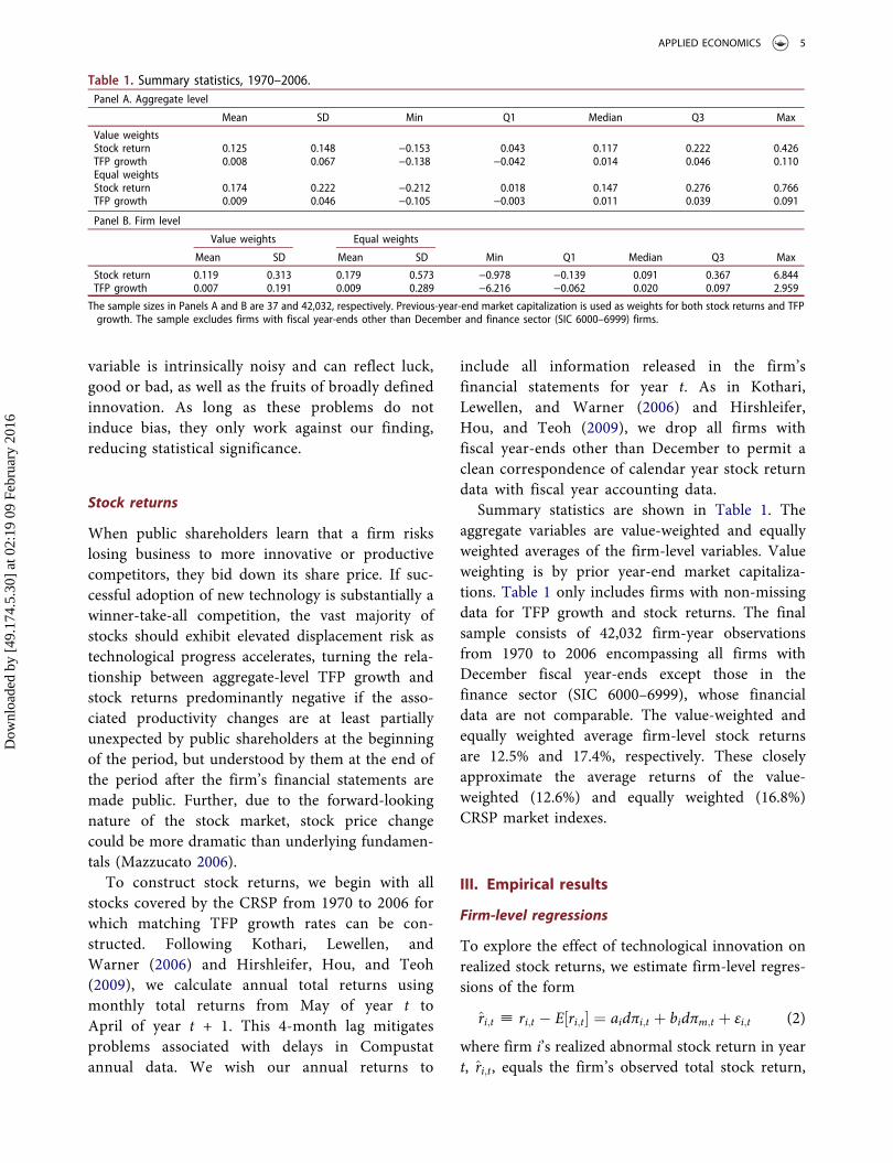
Summary statistics are shown in Table 1. Theaggregate variables are value-weighted and equallyweighted averages of the firm-level variables. Valueweighting is by prior year-end market capitaliza-tions. Table 1 only includes firms with non-missingdata for TFP growth and stock returns. The finalsample consists of 42,032 firm-year observationsfrom 1970 to 2006 encompassing all firms withDecember fiscal year-ends except those in thefinance sector (SIC 6000–6999), whose financialdata are not comparable. The value-weighted andequally weighted average firm-level stock returnsare 12.5% and 17.4%, respectively. These closelyapproximate the average returns of the value-weighted (12.6%) and equally weighted (16.8%)CRSP market indexes.

III. Empirical results

Firm-level regressions

To explore the effect of technological innovation onrealized stock returns, we estimate firm-level regres-sions of the form

r̂i;t ; ri;t � E½ri;t� ¼ aidπi;t þ bidπm;t þ εi;t (2)

where firm i’s realized abnormal stock return in yeart, r̂i;t, equals the firm’s observed total stock return,

Table 1. Summary statistics, 1970–2006.Panel A. Aggregate level

Mean SD Min Q1 Median Q3 Max

Value weightsStock return 0.125 0.148 −0.153 0.043 0.117 0.222 0.426TFP growth 0.008 0.067 −0.138 −0.042 0.014 0.046 0.110Equal weightsStock return 0.174 0.222 −0.212 0.018 0.147 0.276 0.766TFP growth 0.009 0.046 −0.105 −0.003 0.011 0.039 0.091

Panel B. Firm level

Value weights Equal weights

Mean SD Mean SD Min Q1 Median Q3 Max

Stock return 0.119 0.313 0.179 0.573 −0.978 −0.139 0.091 0.367 6.844TFP growth 0.007 0.191 0.009 0.289 −6.216 −0.062 0.020 0.097 2.959

The sample sizes in Panels A and B are 37 and 42,032, respectively. Previous-year-end market capitalization is used as weights for both stock returns and TFPgrowth. The sample excludes firms with fiscal year-ends other than December and finance sector (SIC 6000–6999) firms.

APPLIED ECONOMICS 5

Dow

nloa

ded

by [

49.1

74.5

.30]

at 0

2:19

09

Febr

uary

201

6

ri;t, minus its expected value, E½ri;t�, estimated byCAPM (captial asset pricing model) or other factormodels. TFP growth for individual firm i in year tand aggregate-level TFP growth are denoted dπi;tand dπm;t, respectively, with the latter defined asthe value-weighted average of the dπi;t.

11 Our objec-tive is to measure the correlation between firm i’sabnormal stock return and changes in its economicprofits, which we decompose into two components:the change in its economic profits associated with itsown innovations, dπi;t, and the change in its eco-nomic profits due to either positive or negative spil-lovers associated with the pace of economy-levelinnovation, as captured by bidπm;t.

Because of the inclusion of dπm;t in Equation (2), thecoefficient ai on dπi;t captures the effect of firm i’s firm-specific productivity growth on its own value.12 Theliterature suggests that ai should be positive. Chan,Martin, and Kensinger (1990) report significant positivestock price reactions when firms announce increasedR&D budgets. Pakes (1985) and Blundell, Griffith, andvan Reenen (1999) find higher shareholder value infirms with higher R&D or patents. İmrohoroğlu andTüzel (2014) report a positive relationship betweenfirms’ stock returns and their contemporaneous TFPgrowth, which they interpret as exposure to a technol-ogy risk factor in an asset pricing framework.

The regression coefficient, bi, measures the relation-ship of firm i’s stock return to aggregate TFP growth,above and beyond that to firm i’s own TFP growth.Thus, we assume that the effect of positive or negativespillovers on each firm’s value is proportional to thechange in aggregate economic profits, dπm;t, but allowthe ratio of proportionality to differ across firms. Theexisting literature has ambiguous predictions about bi,the partial correlation of firm i’s stock return withaggregate productivity growth. If positive spillovers pre-dominate, firms’ bi should be largely positive, implying

that most firms’ stock market valuation rise as aggre-gate-level productivity rises; but if negative spilloverspredominate, most firms’ bi should be negative, suggest-ing the negative spillover effect (Tirole 1988; Bena andGarlappi 2012; Gârleanu, Kogan, and Panageas 2012).

To operationalize Equation (2), we estimate thefollowing regression separately for each firm usingannual data windows of various lengths;

ri;t � rf ;t ¼ αi þ aidπi;t þ bidπm;t

þ βi rm;t � rf ;t� �þ εi;t: (3)

In Equation (3), firm i’s expected return compo-nent is rf ;t þ βi rm;t � rf ;t

� �, estimated using the

CAPM with the annualized 1-month treasury bill(T-bill) return, rf ;t, the CRSP value-weighted annualmarket return, rm;t, and stock i’s estimated CAPMbeta, βi.

13 The intercept, αi, captures any remainingunexplained component in the firm’s stock return.

Table 2 summarizes the distributional characteris-tics of the estimated ai and bi thus obtained. The firsttwo columns describe coefficients from regressionsusing all available data for each of the 367 firms forwhich at least 20 observations exist over the sampleperiod of 1970–2006. Numbers in parentheses are thenumber of firms with statistically significant (10%)coefficients. Using long-lived firms only allows moreprecise estimation of the coefficients in Equation (3),but eliminates firms founded after 1986 and thusobviously misses major innovative entrants duringthe 1990s IT boom. We, therefore, rerun Equation(3) for each firm using sequentially increasingly inclu-sive sampling criteria and shorter estimation windows.The third and the fourth columns use 30-year rollingwindows and firms having 20 or more observations;the third pair of columns uses 20-year rolling windowsand firms having 10 or more observations; the fourthpair of columns uses 10-year rolling windows andfirms with five observations or more.14

11The aggregate TFP growth in Equation (2) excludes firm i to prevent spurious correlations between the TFP growth of firm i and the aggregate TFP growth.12Including the lagged value of dπm;t in Equation (2) allows an AR(1) structure in the dπm;t . This lets aggregate TFP growth obey an AR(1) process as well.Given this, bi captures the explanatory power of ‘unexpected’ aggregate TFP growth on firm i’s stock market return. We omit the lagged value as arobustness check and find the distributional characteristics of bi to remain qualitatively similar to that described in the figures and tables.

13Our results are robust to alternative specifications. For example, to avoid any look-ahead bias, we instead use CAPM βis estimated from the prior year’sdata to calculate the abnormal return in Equation (2), and then run regressions of that form. All the results remain qualitatively the same. Replicating thisprocedure using other asset pricing models to calculate the abnormal return in Equation (2) yields qualitatively similar results. See section ‘Robustnesschecks’ for details.

14There is one caveat with the restriction on the number of observations we use in estimating Equation (3). Jovanovic and Rousseau (2001) argue that a newtechnology may induce private firms to list sooner to utilize risk-tolerant equity financing. If new lists prosper on average after IPOs, we may interpret thisas a positive spillover effect of technology innovation. If this is the case, we are underestimating the importance of the positive spillover effect since therestriction on the number of observations may exclude many of new lists. However, Fama and French (2004) report a lower survival rate for new lists inrecent decades. This shows that not all the new entrants enjoy the positive spillover effects of technology innovations, suggesting that new lists alsoconsist of extreme winners and extreme losers (Chun et al. 2008). This reduces the concern for underestimating the positive spillover effect by notincluding them. We thank an anonymous referee for pointing this out.

6 H. CHUN ET AL.

Dow

nloa

ded

by [

49.1

74.5

.30]

at 0

2:19

09

Febr

uary

201

6

First, consider the leftmost two columns, whichsummarize the coefficients for firm-level regression(Equation (3)) for firms having at least 20 annualobservations. Column 2A.1 of Panel A reveals approxi-mately 74% of the firm-level regression coefficients aito be positive. About 27% of the ai coefficients arestatistically significant at 10%, and 87% of these arepositive. Column 2B.1 of Panel B summarizes the ana-logous distributional characteristics for the firm-levelregression coefficients, bi, which gauge the correlationof each firm’s stock return with aggregate TFP growth.Some 81% of firms attract negative bi coefficients.About 28% of the bi are significant, and approximately95% of these are negative. These results show that afirm’s own stock return tends to correlate positively

with its own innovation success, but negatively withthe aggregate innovative success of the economy.15

The second three rows in each panel providemedians as well as equally weighted and value-weighted means of the estimated ai and bi regressioncoefficients. Again focusing on the first pair of col-umns, the equally weighted mean of the ai is 0.575and exceeds its value-weighted analogue of 0.201.The equally weighted mean of the bi is –0.955, andlikewise exceeds its value-weighted analogue of−0.437 in absolute value. These patterns in equallyweighted versus value-weighted means suggest thatsmaller firms profit more from their own innovativesuccesses, but also suffer worse ill effects amid aggre-gate innovative success.

Table 2. Characteristics of coefficients on firm-level TFP growth, aggregate-level TFP growth and the market return in firm-levelregressions explaining firm-level stock return.Panel A. Coefficients on firm’s own TFP growth (ai)

2A.1 2A.2 2A.3 2A.4

Number of coefficientsNegative 94 (13) 678 (85) 3337 (333) 9899 (858)Positive 273 (87) 1991 (573) 8978 (2253) 18,765 (3186)Total 367 (100) 2669 (658) 12,315 (2586) 28,664 (4044)

Median 0.454 (1.066) 0.440 (1.257) 0.477 (1.546) 0.474 (1.871)Mean (EW) 0.575 (1.223) 0.599 (1.329) 0.757 (1.852) 0.882 (2.207)Mean (VW) 0.201 (0.362) 0.234 (0.221) 0.313 (0.298) 0.383 (1.017)

Panel B. Coefficients on aggregate TFP growth (bi)

2B.1 2B.2 2B.3 2B.4

Number of coefficientsNegative 297 (96) 2139 (630) 8598 (1660) 18,000 (2278)Positive 70 (5) 530 (24) 3717 (219) 10,664 (798)Total 367 (101) 2669 (654) 12,315 (1879) 28,664 (3076)

Median −0.974 (−1.998) −0.902 (−2.167) −0.815 (−2.738) −0.797 (−3.237)Mean (EW) −0.955 (−2.105) −0.979 (−2.402) −0.831 (−2.553) −0.730 (−2.132)Mean (VW) −0.437 (−1.211) −0.411 (−1.616) −0.400 (−1.600) −0.295 (−1.335)

Panel C. CAPM beta (βi)

2C.1 2C.2 2C.3 2C.4

Number of coefficientsNegative 54 (1) 506 (27) 3248 (114) 9052 (498)Positive 313 (98) 2163 (587) 9067 (1590) 19,612 (2445)Total 367 (99) 2669 (614) 12,315 (1704) 28,664 (2943)

Median 0.381 (0.762) 0.360 (0.767) 0.360 (1.040) 0.416 (1.345)Mean (EW) 0.448 (0.842) 0.408 (0.820) 0.437 (1.096) 0.468 (1.165)Mean (VW) 0.424 (0.656) 0.436 (0.701) 0.405 (0.858) 0.418 (1.091)

Panel D. Adjusted R2

2D.1 2D.2 2D.3 2D.4

Median 0.082 0.072 0.057 0.068Mean (EW) 0.106 0.097 0.082 0.069Mean (VW) 0.109 0.095 0.096 0.081

Regression coefficients are estimated separately for each firm. The first pair of columns summarizes coefficients from regressions using all available data foreach of the 367 firms with at least 20 observations in the sample window, 1970–2006. Numbers in parentheses are counts of firms with statisticallysignificant (10%) coefficients. The second pair of columns uses 30-year rolling windows and includes firms with 20 or more in the window. The third pair ofcolumns uses 20-year rolling windows and firms with 10 or more observations. The fourth pair of columns uses 10-year rolling windows and firms with fiveobservations or more. Medians, equally weighted (EW) means and value-weighted (VW) means of coefficients are reported in the last three rows of eachpanel. The sample excludes firms with fiscal year-ends other than December and finance sector (SIC 6000–6999) firms.

15Estimating regression for each firm and counting significant coefficients fail to account for cross-firm correlations. An alternative approach, firm-level panelregressions assuming homogeneous ai and bi coefficients across firms and clustering by time, while imposing a different and more restrictive set ofassumptions, reproduces the central findings reported in this section. See section ‘Firm-level panel regressions’ for details.

APPLIED ECONOMICS 7

Dow

nloa

ded

by [

49.1

74.5

.30]

at 0

2:19

09

Febr

uary

201

6

Column 2C.1 of Panel C of Table 2 shows the biand βi coefficients to be very different too. About85% of firm-level regressions attract positive βi coef-ficients, indicating that firms’ stock returns typicallycorrelate positively with market returns. This alsoconfirms that the market risk premium and aggre-gate TFP growth rate have different effects on stockreturns. About 27% of the βi are significant, and ofthese some 99% are positive. The equally weightedand value-weighted means of the βi are similar: 0.448and 0.424, respectively. The low means of the βireflect Compustat’s more limited coverage of smallerfirms and our requirement that firms to have acertain number of years of data, depending on theestimation window, removing younger firms fromthe sample.

The coefficients summarized in the first pair ofcolumns arise from regressions using a single longwindow from 1970 to 2006 for each firm and usingonly firms having least 20 observations. This pre-sumes constant regression coefficients over time foreach individual firm. To let each firm’s ai and bi varyover time, we rerun Equation (3) using alternativewindows and inclusion criteria. The other columnsin Table 2 summarize regression coefficients esti-mated using 30-year rolling windows with at least20 observations, 20-year rolling windows with atleast 10 observations and 10-year rolling windowswith at least 5 observations.16 Decreasing the size ofthe estimation window, while increasing the numberof firms we can use, decreases the number of obser-vations in each window used in estimating Equation(3) for each firm, reducing the fraction of coeffi-cients attaining significance. Nonetheless, the basicpattern of predominantly positive ai and predomi-nantly negative bi persists throughout the table. Forexample, column 2B.2 of Panel B, summarizing thebi coefficients for 30-year rolling windows with atleast 20 observations, shows approximately 80% ofthe bi coefficients negative. About 25% of these areflagged for statistical significance and about 96% ofthese are negative. Column 2B.3 of Panel B, describ-ing coefficients estimated in 20-year rolling windowswith at least 10 observations, shows approximately

70% of the bi coefficients negative. About 15% ofthese are flagged for statistical significance, andamong these, some 88% are negative. Lastly, column2B.4 of Panel B describes results from 10-year rollingwindows with at least five observations. It showsapproximately 63% of the bi coefficients to be nega-tive. About 11% of them are flagged as statisticallysignificant and about 74% of these are negative.Thus, the 10-year windows entirely obviate statisticalsignificance: 11% (3076 of 28,664 coefficients) –essentially the expected 10% incidence of Type IIerrors – are flagged for significance at 10%.However, Type II errors should be 50%, not 74%,negative, leaving even these runs suggestive of nega-tive spillovers.

Panels A and B of Figure 1 graph the distributionof the firm-level regression ai and bi coefficients,respectively, estimated using 10-year rollingwindows.17 Panels A1 and B1 include all estimatedcoefficients, while Panels A2 and B2 include onlycoefficients that are significant at 10% or better.The distributions of the ai and bi differ starkly, anda significantly larger negative mass in the bi distribu-tion is apparent.

If bi captures negative spillovers from aggregateproductivity growth, the distribution characteristicsof the bi should vary over time as aggregate produc-tivity growth accelerates and slows. Schumpeter(1939) posits that, as a major innovation first spreadsacross the economy, successful innovators far outpaceeach affected industry’s increasingly troubled incum-bents; but that once the innovation has propagatedfully, and its best uses in each industry become appar-ent, an increasingly homogeneous set of survivingfirms should compete increasingly on price, ratherthan new product or process development, causingprofit rates should decline towards relatively low andhomogenous levels. This thesis suggests a period ofwidening performance gaps as a new technologyspreads followed by a period of narrowing perfor-mance gaps as it grows mature. Chun, Kim, andMorck (2011) show firm-performance heterogeneityamong U.S. firms increasing until the end of the 20thcentury, but decreasing thereafter, and link this more

16Rolling windows induce serial correlation in firm’s estimated coefficients in addition to the cross-firm correlations within windows (previous footnote). Analternative approach, panel regressions (section ‘Firm-level panel regressions’), is more restrictive in assuming homogeneous ai and bi coefficients acrossfirms and windows, but allows two-dimensional clustering (Thompson 2011) to reflect both cross-firm and time-series non-independence. This exerciseconfirms the findings in this section.

17We obtain similar figures for other estimation windows as well.

8 H. CHUN ET AL.

Dow

nloa

ded

by [

49.1

74.5

.30]

at 0

2:19

09

Febr

uary

201

6

precisely to the observed patterns of IT propagationin different industries. Pástor and Veronesi (2009)likewise interpret changing stock return volatility toconclude that the diffusion of IT was essentially com-plete in the United States by about 2002. Kogan et al.(2012) show that firms affected negatively by otherfirms’ patents in the short run, generally eventuallybenefit from them in the long run – if they survive theinitial negative shock. These considerationssuggest specific patterns of time-series variation inthe distribution characteristics of the bi, for whichwe can test.

Panels A and B of Figure 2 summarize how distri-bution characteristics of the ai and bi change over timeby plotting their decile cut-offs over successive 10-yearrolling windows, each ending in the indicated year.The rightmost graphs in each panel plot differencesbetween the distributions’ 9th and 1st decile cut-offs.

Panel A of Figure 2 shows that, consistent withTable 2, the positive masses of the ai greatly out-weigh their negative masses throughout. Moreover,while their distributions narrow somewhat in the1990s, their medians remain positive throughout.In contrast, the distributional characteristics of the

Panel A1 Panel A2

Panel B1 Panel B2

Panel C1 Panel C2

0.1

.2.3

.4D

ensi

ty

–10 –5 0 5 10 15

a

0.1

.2.3

.4D

ensi

ty

–10 –5 0 5 10 15

a

0.1

.2D

ensi

ty

–20 –10 0 10 20b

0.1

.2D

ensi

ty

–20 –10 0 10 20

b

0.1

.2.3

.4.5

Den

sity

–5 0 5 10beta

0.1

.2.3

.4.5

Den

sity

–5 0 5 10beta

Figure 1. Distributions of firms’ stock return responses to own and aggregate TFP growth: Panel A1. Firm-level TFP: all firms; PanelA2. Firm-level TFP: significant at 10%; Panel B1. Aggregate TFP: all firms; Panel B2. Aggregate TFP: significant at 10%; Panel C1.CAPM beta: all firms; Panel C2. CAPM beta: significant at 10%.Figures omit top and bottom 1% of estimated coefficients.

APPLIED ECONOMICS 9

Dow

nloa

ded

by [

49.1

74.5

.30]

at 0

2:19

09

Febr

uary

201

6

bi change markedly with time. Panel B of Figure 2shows that the median bi remains negative, except inwindows ending near the turn of the century, whenthe distribution of significant coefficients (Panel B2)both shifts its median into the positive range anddistends its positive tail before reverting to its earlierform in later windows.

Panel A3 of Figure 2 shows the difference between9th and 1st decile cut-offs of the ai to be relativelystable throughout the sample period. Again, thiscontrasts starkly with the distributions of the bi.Panel B3 of Figure 2 shows the difference between9th and 1st decile cut-offs of the bi increasing untilthe end of the 20th century, and then decreasing.The increasingly positive median of firm’s bi might

reflect positive spillovers slowly overtaking negativespillovers as the new IT ran its course, but mightalso reflect generally upward biased stock returns asthe 1990s dot.com bubble expanded. Regardless,most of the 1990s show predominantly negative biand the entire decade, even during the bubble per-iod, exhibits a widening performance gap betweensharply divided winners and losers as IT-relatedinnovation peaked (Jovanovic and Rousseau 2005).

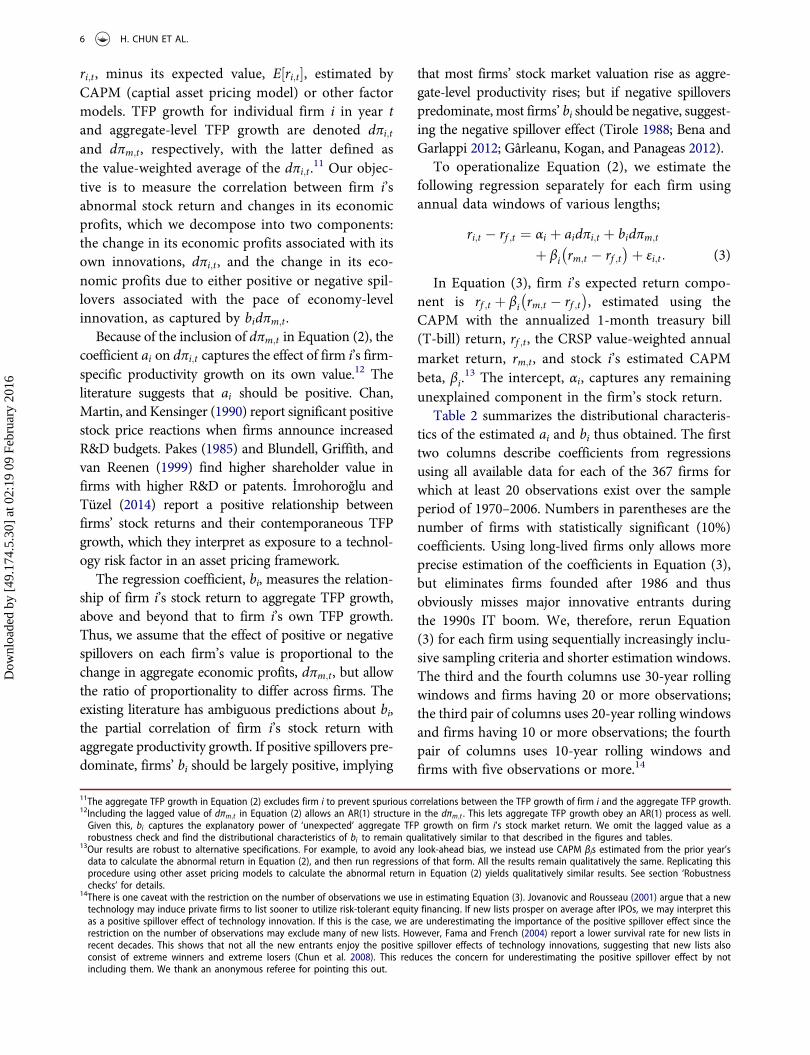
Figure 3 reports the empirical probability func-tions of firms’ bi, averaged across 1980–2006, byindustry. The complete distributions of the bi exhibitnegative medians in 42 of 44 industries, and thedistributions of the significant bi (not shown) arelikewise negative in 38 of 43 industries.18 Figure 3

Panel A1 Panel A2 Panel A3

Panel B1 Panel B2 Panel B3

–5.0

–2.5

0.0

2.5

5.0

7.5

1980 1985 1990 1995 2000 2005–10

–5

0

5

10

15

1980 1985 1990 1995 2000 20050

2

4

6

8

10

12

0

1

2

3

4

5

6

7

1980 1985 1990 1995 2000 2005

All firms (left axis)

Significant at 10% (right axis)

–10

–5

0

5

10

15

1980 1985 1990 1995 2000 2005–20

–10

0

10

20

30

1980 1985 1990 1995 2000 20050

5

10

15

20

25

30

0

2

4

6

8

10

12

14

16

1980 1985 1990 1995 2000 2005

All firms (left axis)

Significant at 10% (right axis)

Figure 2. Dispersion in firm-level stock return responses to own and aggregate TFP growth: Panel A1. Firm-level TFP: all firms; PanelA2. Firm-level TFP: Significant at 10%; Panel A3. Firm-level TFP: 90 percentile minus 10 percentile; Panel B1. Aggregate TFP: all firms;Panel B2. Aggregate TFP: Significant at 10%; Panel B3. Aggregate TFP: 90 percentile minus 10 percentile.Figures show distributions of decile cut-offs for coefficients on firm and aggregate TFP growth obtained from Equation (3) that areestimated over 10-year windows for each firm. In Panels A1, A2, B1 and B2, the three black lines, from the bottom up, track 10th,50th (median) and 90th percentiles, respectively, by the end-year of each 10-year estimation window. Grey lines representintermediate deciles. Panels A1 and B1 include all firms and Panels A2 and B2 include only firms with coefficients significant at 10%.

18One sector lacks significant coefficients.

10 H. CHUN ET AL.

Dow

nloa

ded

by [

49.1

74.5

.30]

at 0

2:19

09

Febr

uary

201

6

shows that the negative coefficients of bi in Figure 2are not concentrated within a few industries, but arecharacteristic of firms spread across the economy asa whole. Repeating this exercise, but separating man-ufacturing from non-manufacturing firms, yieldssimilar patterns (not shown) revealing the patternto be common across both broad sectors.

The findings in this section are consistent withstock returns reflecting Schumpeter’s (1912) creativedestruction. The thick positive tail of the ai distribu-tion reflects profits from firms’ own innovationsboosting their own share prices. The thin positivetail of the bi distribution is consistent with a few

‘winners’ benefiting hugely from aggregate produc-tivity growth, while the thicker negative tail is con-sistent with most firms being left behind bytechnological progress.

Aggregate-level regressions

To explore the relationship between the stock mar-ket return reacts and aggregate productivity growth,we regress the stock market return on aggregate TFPgrowth.

rm;t ¼ aþ bdπm;t þ εm;t: (4)

0 0.25 0.5 0.75 1

PetroleumFarmsHotels

Water transportationOil extraction

Amusement servicesElectric and gas services

Radio and TVTransportation services

WholesalesHealth services

Engineering servicesIndustrial machinery

TelephoneFabricated metal

Tobacco productsElectronics

FoodBusiness services

InstrumentsConstructionCoal mining

LeatherEducational services

ApparelNonmetallic minerals

Metal miningLumber & wood

Miscellaneous manufacturingTrucking

Primary metalPrinting & publishing

ChemicalsFurniture & fixtures

Transportation by airPersonal servicesRubber & plastics

RetailsMotion pictures

Stone, clay, & glassTransportation equipment

PaperRailroad

Textile

Figure 3. Fraction of firms with negative stock return response to value-weighted aggregate TFP growth, means over 1980–2006by industry.Each bar indicates the proportion of firms with negative stock return responses to aggregate TFP growth in Equation (3), averagedover the sample period of 1980–2006. The sample includes all industries with three or more firms in 1980–2006.

APPLIED ECONOMICS 11

Dow

nloa

ded

by [

49.1

74.5

.30]

at 0

2:19

09

Febr

uary

201

6

This specification follows from summing theregressions (Equation (2)) across all firms, weightingeach by wi.

19 The coefficient b, which captures thelinkage between the stock market return and aggre-gate TFP growth, is simply the weighted average ofthe bi in Equation (2). Thus, if positive spilloversoutweigh negative spillovers across firms, theweighted average b ;

Piwibi > 0; but if the negative

spillover effect predominates, b < 0.20 Moreover, ifthe distributional characteristic of the firm-level bidiffers for different estimation windows, b can varythrough time, and even flip signs.

Panel A in Table 3 summarizes these regressionsof (aggregate) stock market returns, rm;t, on aggre-gate TFP growth, dπm;t, taking aggregates as meansof firm-level stock returns and TFP growth rates,respectively. The table displays regressions usingvalue-weighted as well as equally weighted means.Firm-level stock returns are always measured fromMay of year t to April of year t + 1.

Regressions 3A.1 and 3A.2 show dπm;t definedhere as the value-weighted mean TFP growth rate,attracting a significantly negative coefficient.Regression 3A.2 shows that including lagged TFP

Table 3. Regressions of stock returns on TFP growth: aggregate-level versus firm-level panel regressions, 1970–2006.Panel A. Aggregate level

3A.1 3A.2 3A.3 3A.4

VW aggregate TFP −0.622* −0.649*(0.359) (0.357)

Lagged VW aggregate TFP 0.462(0.358)

EW aggregate TFP −1.385* −1.557*(0.772) (0.802)

Lagged EW aggregate TFP 0.677(0.802)

Constant 0.129*** 0.126*** 0.186*** 0.181***(0.024) (0.024) (0.036) (0.037)

Sample size 37 37 37 37Adj. R2 0.079 0.122 0.084 0.103

Panel B. Firm level

3B.1 3B.2 3B.3 3B.4 3B.5 3B.6

Firm TFP 0.289*** 0.289*** 0.291*** 0.296*** 0.253*** 0.261***(0.026) (0.025) (0.026) (0.027) (0.025) (0.025)

Lagged firm TFP 0.019 0.024 0.035(0.017) (0.014) (0.022)

VW aggregate TFP −1.175*** −1.129***(0.343) (0.325)

Lagged VW aggregate TFP 0.788**(0.324)

EW aggregate TFP −1.657** −1.872***(0.697) (0.620)

Lagged EW aggregate TFP 1.113***(0.358)

CAPM factor 0.592*** 0.606*** 0.679*** 0.701*** 0.636*** 0.636***(0.150) (0.126) (0.174) (0.158) (0.176) (0.175)

Sample size 42,032 42,032 42,032 42,032 42,032 42,032Adj. R2 0.092 0.100 0.090 0.098 0.074 0.074

Dependent variables in Panel A are value-weighted (VW) aggregate stock returns (columns 3A.1 and 3A.2) or equally weighted (EW) aggregate stock returns(columns 3A.3 and 3A.4). The dependent variable in Panel B is firm-level stock returns. Panel regressions in Panel B include firm-fixed effects. The sampleexcludes firms with fiscal year-ends other than December and finance sector (SIC 6000–6999) firms. Numbers in parentheses are standard errors. Standarderrors in Panel B are year-clustered.

*Significant at the 10% level.**Significant at the 5% level.***Significant at the 1% level.

19Summing both sides of Equation (2), weighting by wi = firm i’s prior year-end market capitalization, yieldsPiwibri ; rm;t � E rm;t

� � ¼Piwiaidπi;t þ dπm;t

Piwibi . This leads to Equation (4) only if a ; E rm;t

� �þPiwiaidπi;t is a constant within each sample period. This would follow if

both E rm;t� �

andPiwiaidπi;t were constant. Empirically, E rm;t

� �need not be constant (Campbell, Lo, and MacKinlay 1997) and

Piwiaidπi;t need not be

zero – although E dπi;t� �

is fairly close to zero (between 0.7% and 0.9% in Table 1). Nonetheless, if there is little time variation inPiwibi within estimation

windows, Equation (4) serves as a parsimonious specification. A comparison of point estimates, shown below, reveals that b ffi Piwibi in corresponding

estimation window, validating the assumption of a constant a in each window.20If a few very large firms had bi > 0, a positive b might ensue despite most firms having bi < 0. However, equally weighted and value-weighted means ofthe bi exhibit similar behaviour (see especially Figure 4).

12 H. CHUN ET AL.

Dow

nloa

ded

by [

49.1

74.5

.30]

at 0

2:19

09

Febr

uary

201

6

growth as a control leaves this result qualitativelyunchanged.21 Regressions 3A.3 and 3A.4 repeatthese exercises, but define dπm;t as an equallyweighted mean TFP growth rate. The point estimatesfor b remain negative and significant, and roughlydouble in magnitude. Table 3 thus suggests thatnegative spillovers outweigh positive spillovers inthe aggregate for the firms in our sample.

To explore the stability of b over time, Figure 4 plotsestimates of the b coefficient from Equation (4) oversuccessive 10-year rolling windows against the win-dows’ end-years. The figure also plots the value-weighted and equally weighted means of the firm-level coefficients bi from regressions (Equation (3))estimated using the same rolling windows. These twoseries of means closely follow the aggregate-levelregression coefficients b, though the equally weightedmean of the firm-level coefficients bi is generally morenegative than its value-weighted analogue, especiallyfor windows ending after 2000. These patterns suggestthat the time variation in b might be associated with avarying preponderance of negative firm-level coeffi-cients bi estimated using different windows.

Firm-level panel regressions

The previous sections show that firm-level stockreturns are generally positively associated with firms’own productivity growth, but generally negatively asso-ciated with aggregate TFP growth. That is, in Equation(3), the ai are generally positive and the bi are generallynegative. Moreover, the aggregate productivity growthcoefficient b in Equation (4) closely tracks the means ofthe firm-level coefficients on aggregate productivitygrowth, bi, in Equation (2), operationalized asEquation (3). These patterns suggest the alternativespecification of panel regressions of the form

ri;t ¼Xi

δi þ adπi;t þ bdπm;t þ εi;t (5)

with ri,t and dπi,t the stock return and TFP growthrate, respectively, of firm i in year t, and with δirepresenting firm-fixed effects. Including aggregateTFP growth, dπm,t, in the regression precludes time-fixed effects.

The advantage of the firm-by-firm regressions inthe previous section is that each firm has a distinctset of coefficients, ai and bi, for each firm andwindow,22 allowing an analysis of their distributionalcharacteristics. However, spillovers complicateassessment of the overall significance of the coeffi-cients ai and bi across many firms by inducing cross-firm correlations within a given window and, asnoted above, coefficients estimated using overlap-ping windows may not be independent. The panelspecification (Equation (5)), though more restrictivein requiring the firm-level coefficients in Equation(3) to be identical across firms and across time(ai = a and bi = b for each i in the whole sample),23

permits clustering by year (to allow for cross-firmstatistical dependence) or by firm (to address persis-tence in data for each firm). Both these considera-tions weigh against finding statistical significance inEquation (5). Standard errors with firm clusteringare smaller, thus generating higher t-statistics thanthose with year clustering, a typical characteristic ofasset pricing data (Petersen 2009). Clustering by firmor by firm and year simultaneously (Thompson

–3

–2

–1

0

1

2

3

1980 1985 1990 1995 2000 2005

Aggregate response

Value-weighted average of firm-level responses

Equally weighted average of firm-level responses

Figure 4. Aggregate-level versus mean firm-level stock returnresponses to aggregate TFP growth in rolling 10-year windowsending in the year indicated.A black line is aggregate response coefficients obtained fromEquation (4) over 10-year rolling windows. Grey and dottedlines are value-weighted and equally weighted averages offirm-level responses, respectively, obtained from firm-levelregressions in Equation (3) that are estimated over 10-yearwindows for each firm.

21Here and throughout, we define qualitatively unchanged to mean an identical pattern of signs and significance and point estimates of roughly comparablemagnitude. This specification lets aggregate TFP growth obey an AR(1) process, thereby letting b gauge the importance of plausibly ‘unexpected’ TFPgrowth in regressions explaining the stock market return.

22More precisely, we estimate aτi and bτi for each firm i and for each estimation window τ. For brevity, τ is suppressed in our notation.23Kogan et al. (2012) run similar firm-level panel regressions to examine the negative spillover effect. Their aggregate innovation measure, an economicimportance-weighted average of other firms’ patents, attracts a significant negative coefficient, also consistent with the negative spillover effect.

APPLIED ECONOMICS 13

Dow

nloa

ded

by [

49.1

74.5

.30]

at 0

2:19

09

Febr

uary

201

6

2011) generates significance levels for a and b vir-tually identical to those obtained from clustering byyear only. Thus, we evaluate the statistical signifi-cance of our estimated coefficients using yearclustering.

Panel B of Table 3 presents these results.Regression 3B.1 shows a firm’s stock return signifi-cantly positively correlated with its own firm-levelTFP growth, but significantly negatively correlatedwith value-weighted aggregate TFP growth.Regression 3B.2 shows these results unaffected byincluding lagged value-weighted aggregate TFPgrowth as a control. Regressions 3B.3 and 3B.4repeat these specifications, but use equally weightedaggregate TFP growth and, in 3B.4, its lagged value,along with firm-level TFP growth. Firm-level TFPgrowth again attracts a significant positive coeffi-cient, and equally weighted aggregate TFP growthagain attracts a negative coefficient.

Importance of spillover effect

This section evaluates the importance of aggregateTFP growth in explaining contemporaneous stockreturns at the firm level. This entails running regres-sions of the form

ri;t � rf ;t ¼ αi þ aidπi;t þ βi rm;t � rf ;t� �þ εi;t (6)

removing aggregate TFP growth from the baselinemodel of Equation (3). By comparing the coefficientestimates of ai and adjusted R2 in Equations (3) and(6), we can assess the importance of the contributionof aggregate TFP growth in explaining contempora-neous firm-level stock return.

Table 4 shows the ai estimates in Equation (6) tobe generally smaller than those in Equation (3).Thus, the median ai estimate based on the wholesample is 0.454 in Equation (3), but only 0.258 inEquation (6). Both the equal-weighted and value-weighted mean ai estimates are also smaller: respec-tively, 0.404 and 0.100 for Equation (6) versus 0.575and 0.201 for Equation (3). The adjusted R2 statisticstell a similar story: the median regression R2 basedon the whole sample is 8.2% for Equation (3), butonly 4.7% for Equation (6), the difference indicatinga roughly 74% increase in goodness of fit fromincluding aggregate TFP growth. The equal-weightedand value-weighted means of the regression R2sare also markedly lower without aggregate TFPgrowth: 7.1% and 8.8%, respectively, for Equation(6) versus 10.6% and 10.9% for Equation (3).Similar patterns emerge using other estimation

Table 4. Alternative specification for firm-level regressions explaining firm-level stock return: excluding aggregate-level TFP growth.Panel A. Coefficients on firm’s own TFP growth (ai)

4A.1 4A.2 4A.3 4A.4

Number of coefficientsNegative 122 (17) 819 (99) 3635 (363) 10,126 (877)Positive 245 (66) 1850 (430) 8680 (1962) 18,538 (3115)Total 367 (83) 2669 (529) 12,315 (2325) 28,664 (3992)Median 0.258 (0.881) 0.284 (1.067) 0.380 (1.469) 0.388 (1.731)Mean (EW) 0.404 (1.048) 0.438 (1.152) 0.651 (1.739) 0.710 (2.051)Mean (VW) 0.100 (0.203) 0.117 (0.148) 0.187 (0.217) 0.233 (0.427)

Panel B. CAPM beta (βi)

4B.1 4B.2 4B.3 4B.4

Number of coefficientsNegative 40 (1) 437 (19) 2860 (85) 8065 (387)Positive 327 (105) 2232 (660) 9455 (1923) 20,599 (3063)Total 367 (106) 2669 (679) 12,315 (2008) 28,664 (3450)Median 0.406 (0.753) 0.401 (0.783) 0.425 (1.071) 0.495 (1.438)Mean (EW) 0.485 (0.856) 0.455 (0.864) 0.510 (1.159) 0.639 (1.442)Mean (VW) 0.447 (0.618) 0.459 (0.728) 0.450 (0.892) 0.520 (1.281)

Panel C. Adjusted R2

4C.1 4C.2 4C.3 4D.4

Median 0.047 0.040 0.025 0.016Mean (EW) 0.071 0.067 0.060 0.057Mean (VW) 0.088 0.080 0.075 0.077

Regression coefficients are estimated separately for each firm. The first pair of columns summarizes coefficients from regressions using all available data foreach of the 367 firms with at least 20 observations in the sample window, 1970–2006. Numbers in parentheses are counts of firms with statisticallysignificant (10%) coefficients. The second pair of columns uses 30-year rolling windows and includes firms with 20 or more in the window. The third pair ofcolumns uses 20-year rolling windows and firms with 10 or more observations. The fourth pair of columns uses 10-year rolling windows and firms with fiveobservations or more. Medians, equally weighted (EW) means and value-weighted (VW) means of coefficients are reported in the last three rows of eachpanel. The sample excludes firms with fiscal year-ends other than December and finance sector (SIC 6000–6999) firms.

14 H. CHUN ET AL.

Dow

nloa

ded

by [

49.1

74.5

.30]

at 0

2:19

09

Febr

uary

201

6

windows. This exercise suggests that omitting theaggregate TFP growth lowers the point estimates ofai and underestimating the explanatory power oftechnology shocks on stock returns.

An alternative approach gauges the importance ofaggregate TFP growth in the firm-level panel regres-sion model of Equation (5). The results, reported inthe last two columns of Panel B of Table 3, reinforceTable 4. For example, the adjusted R2 rises from7.4% to about 9.2% when aggregate TFP growth isincluded, representing a significant increase of about25% in goodness of fit.

Robustness checks

The results in the tables and figures survive a batteryof robustness tests. In all cases, qualitatively similarresults means identical patterns of signs and signifi-cance to those in the tables and point estimates ofroughly comparable magnitudes. Details are pro-vided wherever this is not true.

The regressions in the tables utilize simple CAPMestimates of each stock’s return each period. Werepeat all these regressions using each of the follow-ing alternative specifications,

ri;t ¼ αi þ aidπi;t þ bidπm;t þ βi rm;t � rf ;t� �þ εi;t

(7A)

ri;t ¼ �ri þ aidπi;t þ bidπm;t þ εi;t (7B)

ri;t � rf ;t ¼ αi þ aidπi;t þ bidπm;t þX3f¼1

λi;f ff þ εi;t

(7C)

ri;t � rf ;t ¼ αi þ aidπi;t þ bidπm;t þ cidπjðiÞ;tþ βi rm;t � rf ;t

� �þ εi;t: (7D)

Specification (Equation (7A)) uses Black’s (1972)zero-beta model in lieu of the CAPM; Equation (7B)employs a naïve specification in which each firm’sexpected stock return is assumed constant; Equation(7C) uses the Fama–French (1993) three-factor model.Equation (7D) includes the industry-level TFP variable,dπjðiÞ;t, the value-weighted average of the TFP growthrates of all firms in j(i), the industry firm i belongs. Anintermediate level of aggregation, industry-level data,might be of interest for several reasons. This removesany potential impact industry-level TFP growth might

have on the coefficients of own firm-level TFP growth,ai, and aggregate TFP growth, bi.

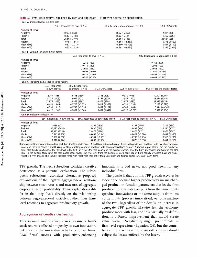
Table 5 shows the distributional characteristics ofthe estimated response coefficients based on alterna-tive specifications described above. Qualitatively simi-lar results to those in Table 2 ensue in all cases. ForEquation (7D), the ci, like the bi, have distributionalcharacteristics consistent with winner-take-all compe-tition. Roughly 56% of firms attract a negative cicoefficient, whereas about 60% attract negative bicoefficients in this specification. However, the greaterincidence of positive ci than bi coefficients is alsosuggestive of relatively more positive spillovers withinthan between industries – perhaps because firms in anindustry use more closely related technologies (Jaffe1986; Bloom, Schankerman, and van Reenen 2013).

We generally aggregate firm-level response vari-ables weighting by market capitalization. Usingequal weighting generates qualitatively similarresults. Weighting by assets or sales, rather thanmarket capitalization also generates results qualita-tively similar to those shown.

We drop observations for all firms with fiscal yearsending in months other than December throughout sothat the stock returns and accounting data, from whichwe construct TFP growth rates, match precisely. If weinclude all firms irrespective of their fiscal years end-ing, for example, the number of firms (firm-year obser-vations) increased from 4672 (42,032) to 9389 (87,106)in the sample period. Rerunning our tests using allavailable data yields qualitatively similar results.

Finally, we consider alternative methods of calculat-ing TFP. Basu and Fernald (1997) and Syverson (2004)modify the standard TFP calculation to account forfirms not fully deploying their capital assets duringbusiness cycle downturns. This approach assumesmaterials and capital-in-production to be imperfectsubstitutes. Hall (1988) proposes a second alternativeTFP calculation using revenue (rather than cost)shares. This approach imposes constant returns toscale. Both alternative TFP measures generate resultsqualitatively similar to those in the figures and tables.

IV. Alternative explanations

The results above expose a fallacy of composition. Afirm’s stock return is positively correlated with itsfirm-level TFP growth rate; but the stock marketreturn is negatively correlated with aggregate-level

APPLIED ECONOMICS 15

Dow

nloa

ded

by [

49.1

74.5

.30]

at 0

2:19

09

Febr

uary

201

6

TFP growth. The next subsection considers creativedestruction as a potential explanation. The subse-quent subsections reconsider alternative proposedexplanations of the negative aggregate-level relation-ship between stock returns and measures of aggregatecorporate sector profitability. These explanations dif-fer in that they focus directly on the relationshipbetween aggregate-level variables, rather than firm-level reactions to aggregate productivity growth.

Aggregation of creative destruction

This seeming inconsistency arises because a firm’sstock return is affected not just by its own innovation,but also by the innovative activity of other firms.Rival firms’ success with productivity-enhancing

innovations is bad news, not good news, for anyindividual firm.

The puzzle is that a firm’s TFP growth elevates itsstock price because higher productivity means chan-ged production function parameters that let the firmproduce more valuable outputs from the same inputs(product innovation) or the same outputs from lesscostly inputs (process innovation), or some mixtureof the two. Regardless of the details, an increase inaggregate TFP growth likewise lets the economyproduce more with less, and this, virtually by defini-tion, is a Pareto improvement that should createvalue overall. Negative bi might predominate infirm-level regressions (Equation (3)), but the contri-bution of the winners to the overall economy shouldeclipse the losses suffered by the losers.

Table 5. Firms’ stock returns explained by own and aggregate TFP growth: Alternative specification.Panel A. Unadjusted for risk-free rate

5A.1 Responses to own TFP (a) 5A.2 Responses to aggregate TFP (b) 5A.3 CAPM beta

Number of firmsNegative 10,033 (863) 18,327 (2397) 9314 (488)Positive 18,631 (3111) 10,337 (751) 19,350 (2363)Total 28,664 (3974) 28,664 (3148) 28,664 (2851)Median 0.453 (1.845) −0.864 (−3.287) 0.393 (1.320)Mean (EW) 0.871 (2.213) −0.800 (−2.306) 0.447 (1.142)Mean (VW) 0.358 (1.026) −0.391 (−1.454) 0.395 (0.961)

Panel B. Without including CAPM factor

5B.1 Responses to own TFP (a) 5B.2 Responses to aggregate TFP (b)

Number of firmsNegative 9250 (789) 19,162 (2970)Positive 19,414 (3498) 9502 (702)Total 28,664 (4287) 28,664 (3672)Median 0.498 (1.905) −1.021 (−3.499)Mean (EW) 0.834 (2.166) −0.894 (−2.470)Mean (VW) 0.380 (0.780) −0.404 (−1.763)

Panel C. Including Fama–French three factors

5C.1 Responsesto own TFP (a)

5C.2 Responses toaggregate TFP (b) 5C.3 CAPM beta 5C.4 FF size factor 5C.5 FF book-to-market factor

Number of firmsNegative 8740 (818) 14,838 (1696) 7708 (425) 10,330 (991) 10,401 (1291)Positive 15,135 (2305) 9037 (701) 16,167 (2279) 13,545 (1792) 13,474 (1745)Total 23,875 (3123) 23,875 (2397) 23,875 (2704) 23,875 (2783) 23,875 (3036)Median 0.452 (1.844) −0.705 (−3.033) 0.417 (1.362) 0.231 (1.332) 0.183 (0.790)Mean (EW) 0.790 (1.917) −0.748 (−2.016) 0.462 (1.269) 0.348 (1.089) 0.014 (−0.340)Mean (VW) 0.412 (1.182) −0.427 (−1.363) 0.467 (1.042) −0.226 (−0.617) 0.072 (0.084)

Panel D. Including industry TFP

5D.1 Responses to own TFP (a) 5D.2 Responses to aggregate TFP (b) 5D.3 Responses to industry TFP (c) 5D.4 CAPM beta

Number of firmsNegative 8188 (673) 14,395 (1809) 13,387 (1706) 7315 (430)Positive 15,687 (2686) 9480 (771) 10,488 (916) 16,560 (2077)Total 23,875 (3359) 23,875 (2580) 23,875 (2622) 23,875 (2507)Median 0.541 (2.350) −0.698 (−3.442) −0.422 (−3.380) 0.432 (1.350)Mean (EW) 0.897 (2.600) −0.541 (−1.712) −0.709 (−2.734) 0.510 (1.236)Mean (VW) 1.018 (2.174) −0.093 (0.236) −0.875 (−1.818) 0.451 (1.216)

Response coefficients are estimated for each firm. Coefficients in Panels A and B are estimated using 10-year rolling windows and firms with five observations ormore and those in Panels C and D using for 10-year rolling windows and firms with seven observations or more. Numbers in parentheses are the number offirms statistically significant at the 10% level in the first three rows for each panel and the average coefficient of the firms statistically significant at the 10%level in the bottom three rows for each panel, respectively. The two rows from the bottom of each panel report both equally weighted (EW) and value-weighted (VW) means. The sample excludes firms with fiscal year-ends other than December and finance sector (SIC 6000–6999) firms.

16 H. CHUN ET AL.

Dow

nloa

ded

by [

49.1

74.5

.30]

at 0

2:19

09

Febr

uary

201

6

Reconciling this reasoning with our findingsrequires returning to the discussion of ‘winner-take-all’ competition. This form of competitionbestows huge rewards on a handful of creative win-ner firms, but wreaks devastation upon vastly moreloser firms. This devastation can take several forms.First, shareholders foresee loser firms’ future cashflows falling as innovation-driven competition inten-sifies. Second, shareholders foresee decreases in thevalues of loser firms’ existing physical capital, pro-duction routines and managerial talent – all of whichwere designed for older technology. Third, both ofthe above effects can increase loser firms’ financialand/or operating leverage, which would furthererode share values if shareholders foresee substantialbankruptcy costs. Fourth, a successfully innovativefirm’s profits need not all accrue to its public share-holders if its creative insiders pay themselves anentrepreneurial rent (e.g. patent royalties). All fourconsiderations, given the forward-looking nature ofshare prices, permit immediate price drops in tech-nology loser firms’ stocks to appear disproportio-nately large relative to their immediate productivitydrops. Regardless of the mechanism, some part ofthe Pareto gains from aggregate TFP growth canreadily accrue to people other than the winnerfirms’ public shareholders at the time its TFP growthis observed.

Time-varying discount rates

Kothari, Lewellen, and Warner (2006) note thatstock prices are the expected present discountedvalues of future corporate disbursements, and arguethat, if investors’ discount rates rise sufficientlywhenever aggregate corporate earnings rise, the neteffect might be lower stock market valuations. Thisthesis requires that investors have not just time-varying risk aversions (Fama 1991; Campbell, Lo,and MacKinlay 1997), but they discount futurerisky cash flows more steeply in good times than inbad times. To test their thesis, Kothari, Lewellen, andWarner (2006) construct several discount rateproxies: the 30-day T-bill rate, the differencebetween 10-year and 1-year constant maturity treas-ury rates and the difference between Moody’s Baaand Aaa yields. Because the stock market returncorrelates negatively with aggregate earningsthroughout their sample window, their thesis

predicts positive correlations between their discountrate proxies and aggregate earnings. Their results areinconclusive: aggregate earnings growth correlatessignificantly positively with the T-bill rate, insignif-icantly with the term structure variable and signifi-cantly negatively with the bond risk premiumvariable. Hirshleifer, Hou, and Teoh (2009) conducta similar analysis and arrive at similarly inconclusiveresults. Also, although the relationship between thestock market return and aggregate earnings growthis negative during their sample period, the relation-ship turns positive in part of our longer samplewindow.

Our explanation based on creative destructionand displacement risk can explain the negative rela-tionship between the stock market return and aggre-gate earnings. Suppose average firm earnings growwhile the performance gap between winner and loserfirms’ earnings widens. As noted above, loser firms’stock prices might fall because of the innovation-driven negative spillover effect (their earnings fallas they lose business to more innovative firms orshareholders discount the value of their capital moreheavily). If displacement risk is a systematic riskfactor disproportionately affecting loser firms’stocks, intensified creative destruction could dispro-portionately elevate the discount rates investors useto value loser firms. Thus, our creative destructionexplanation may be an elaboration of the discountrate thesis of Kothari, Lewellen, and Warner (2006)and Hirshleifer, Hou, and Teoh (2009), not a rivalexplanation. If most listed firms are losers in races toadopt new technologies, their discount rates mightincrease in general, as those papers posit. If the paceof innovation picks up and falls off again, the dis-placement risk factor might wax and wane as well,explaining the sign flip we observe.

Other explanations

Hirshleifer, Hou, and Teoh (2009) decompose earn-ings into cash flow and accrual’s components, andshow that the contemporaneous negative relation-ship between earnings growth and stock returns isdriven by accrual rather than cash flow component.We replicate their findings using their sample per-iod, but not outside it. One possibility is that regu-latory reforms around the turn of the 21st centuryaltered the practice of accruals management in ways

APPLIED ECONOMICS 17

Dow

nloa

ded

by [

49.1

74.5

.30]

at 0

2:19

09

Febr

uary

201

6

that somehow reversed the negative relationshipbetween stock market returns and aggregate earn-ings, at least for a time. The details of such anexplanation are not immediately obvious, but theirhypothesis cannot be rejected out of hand.

Sadka and Sadka (2009) posit that investors foreseeaggregate earnings growth more clearly than firm-level earnings growth. If so, firm-level earningswould convey new information and contempora-neously affect stock returns; but aggregate earnings,largely known in advance, would not. InvokingCampbell’s (1991) return decomposition, they derivea negative aggregate-level relationship betweenexpected earnings growth and the expected stockmarket return. This requires that investors demanda lower risk premium whenever they expect positiveearnings growth (Chen 1991) and Sadka and Sadka(2009) present empirical results supporting this.This hypothesis may also be correct; but is notobviously a complete explanation. For example, ifthe predictability of aggregate earnings is a majordriving force for the negative relationship, the posi-tive relationship observed after 2000 suggests adecreased predictability of aggregate earnings dur-ing that period despite institutional reforms toincrease transparency.

We suggest that Okham’s razor favours a time-varying negative spillover effect as the simplestexplanation of not just the fallacy of composition,but also its changing characteristics over time.Nonetheless, we welcome further research into theimportance of earnings management and the differ-ential predictability of aggregate versus firm-levelfundamentals.

V. Conclusions

Aggregate productivity growth, which many macro-economists interpret as good news for the economy,may not be good news for shareholders (Ritter2012). While some firms’ shares do rise with aggre-gate TFP growth, most firms’ shares drop. Thisimplies that high aggregate productivity growth canbe bad news for the shareholders of most firms and,because losers can outweigh winners in the stockmarket as a whole, for shareholders who hold mar-ket portfolio.

The declines in most firms’ share prices associatedwith increased aggregate productivity growth

highlight the economic importance of negative spil-lovers from technological innovation. These pricedrops might reflect either technology laggards facingintensified competition that erodes their earnings andfuture earnings growth opportunities or the marketdiscounting technology laggards’ future earnings moreheavily to reflect their greater risk of being left behind.Our results also support papers emphasizing winner-take-all competitions in corporate sectors, which claimthat handful of winners outperform most firms,destroying their values as empirically.

In firm-level regressions explaining stock returns,the coefficients of aggregate productivity growth arepredominantly negative, while the coefficients of thefirm’s own productivity growth are predominantlypositive. This suggests an explanation for a fallacy ofcomposition that stock returns and earnings growthcorrelate positively in firm-level data, but negativelyin aggregate data (Kothari, Lewellen, and Warner2006). This seeming contradiction is readily explic-able in that earnings and TFP growth both gauge afirm’s ongoing profitability, and merely reflects apreponderance of listed firms’ stock returns correlat-ing negatively with aggregate productivity growth.These negative aggregate effects sum to a negativecorrelation between the market return and aggregateproductivity growth; despite each firm’s stock returncorrelating positively with the firm’s own productiv-ity growth. Unlike alternative explanations, this the-sis also explains observed variation in themagnitudes of these firm-level and aggregate-leveleffects both across firms and over time.

Taken at face value, our empirical findings implya predominantly negative effect of aggregate pro-ductivity growth on the portfolio wealth of highlydiversified public shareholders in the late 20thcentury. This may reflect public shareholdersbeing precluded from diversifying into early stagestart-ups, and even experiencing a significantwealth loss as economy-wide innovations unfold.Our estimation techniques require that we excludevery young firms from the analysis that leads to thisconclusion, so if these firms provide very highreturns, public shareholders might share morefully in the fruits of technological progress.However, younger firms’ post-IPO long-run returnsare negative on average (e.g. Ritter 1998), suggest-ing that holding more younger stocks would nothave left public shareholders wealthier.

18 H. CHUN ET AL.

Dow

nloa

ded

by [

49.1

74.5

.30]

at 0

2:19

09

Febr

uary

201

6

Acknowledgements

We thank Jay Pil Choi, Martin Dierker, Cheol S. Eun, KeweiHou, Mark Huson, Tomohiko Inui, Bong-Soo Lee, VikasMehrotra, Andrei Shleifer and seminar participants atInternational Conference on Asia-Pacific Financial Markets,CESA Bogota, Korea University, National University ofSingapore, Seoul National University Economics Department,Seoul National University Finance Department, SogangUniversity, Western Economic Association Conference,University of Alberta and Yonsei University EconomicsDepartment. We are also most grateful to the editor and twoanonymous referees for their particularly helpful comments.Earlier version of this article is also available as NBER workingpaper No. 19462.

Disclosure statement

No potential conflict of interest was reported by the authors.

Funding

This work was supported by the National ResearchFoundation of Korea [NRF-2013 S1 A3 A2053312];Institute of Finance and Banking (Seoul NationalUniversity); Institute of Management Research (SeoulNational University). Morck gratefully acknowledges thesupport from the SSHRC and the Bank of Canada.

References

Aghion, P., R. Blundell, R. Griffith, P. Howitt, and S. Prantl.2009. “The Effects of Entry on Incumbent Innovation andProductivity.” Review of Economics and Statistics 91 (1):20–32. doi:10.1162/rest.91.1.20.

Aghion, P., and P. Howitt. 1992. “A Model of Growththrough Creative Destruction.” Econometrica 60 (2): 323–351. doi:10.2307/2951599.

Basu, S., and J. G. Fernald. 1997. “Returns to Scale in U.S.Production: Estimates and Implications.” Journal ofPolitical Economy 105 (2): 249–283. doi:10.1086/262073.

Bena, J., and L. Garlappi. 2012. “Corporate Innovation andReturns.” University of British Columbia Working Paper,Vancouver.

Bessen, J., and M. Meurer. 2008. Patent Failure. Princeton:Princeton University Press.

Black, F. 1972. “Capital Market Equilibrium with RestrictedBorrowing.” The Journal of Business 45 (3): 444–455.doi:10.1086/jb.1972.45.issue-3.

Bloom, N., R. Sadun, and J. van Reenen. 2012. “TheOrganization of Firms across Countries.” The QuarterlyJournal of Economics 127 (4): 1663–1705. doi:10.1093/qje/qje029.

Bloom, N., M. Schankerman, and J. van Reenen. 2013.“Identifying Technology Spillovers and Product MarketRivalry.” Econometrica 81 (4): 1347–1393. doi:10.3982/ECTA9466.

BLS (Bureau of Labor Statistics). 1997. BLS Handbook ofMethods. Washington, DC: Bureau of Labor Statistics.

Blundell, R., R. Griffith, and J. van Reenen. 1999. “MarketShare, Market Value and Innovation in a Panel of BritishManufacturing Firms.” Review of Economic Studies 66 (3):529–554.

Campbell, J. Y., A. W. Lo, and C. MacKinlay. 1999. TheEconometrics of Financial Markets. Princeton: PrincetonUniversity Press.

Campbell, J. Y. 1991. “A Variance Decomposition for StockReturns.” The Economic Journal 101 (405): 157–179.doi:10.2307/2233809.

Chan, L. K., J. Lakonishok, and T. Sougiannis. 2001. “TheStock Market Valuation of Research and DevelopmentExpenditures.” The Journal of Finance 56 (6): 2431–2456.doi:10.1111/jofi.2001.56.issue-6.

Chan, S. H., J. D. Martin, and J. W. Kensinger. 1990.“Corporate Research and Development Expenditures andShare Value.” Journal of Financial Economics 26 (2): 255–276. doi:10.1016/0304-405X(90)90005-K.

Chen, N.-F. 1991. “Financial Investment Opportunities andthe Macroeconomy.” The Journal of Finance 46 (2): 529–554. doi:10.1111/j.1540-6261.1991.tb02673.x.

Chun, H., J.-W. Kim, and J. Lee. 2015. “How DoesInformation Technology Improve AggregateProductivity? A New Channel of Productivity Dispersionand Reallocation.” Research Policy 44 (5): 999–1016.doi:10.1016/j.respol.2014.11.007.

Chun, H., J.-W. Kim, and R. Morck. 2011. “VaryingHeterogeneity among U.S. Firms: Facts andImplications.” Review of Economics and Statistics 93 (3):1034–1052. doi:10.1162/REST_a_00099.

Chun, H., J.-W. Kim, R. Morck, and B. Yeung. 2008.“Creative Destruction and Firm-specific PerformanceHeterogeneity.” Journal of Financial Economics 89 (1):109–135. doi:10.1016/j.jfineco.2007.06.005.

Cohen, W. M., R. R. Nelson, and J. P. Walsh. 2000. ProtectingTheir Intellectual Assets: Appropriability Conditions andWhy U.S. Manufacturing Firms Patent (or Not). NBERWorking Paper No. 7552. Cambridge, MA: NationalBureau of Economic Research.

DeAngelo, H., and R. Roll. 2015. “How Stable Are CorporateCapital Structures?” Journal of Finance 70 (1): 373–418.

Fama, E. F. 1991. “Efficient Capital Markets: II.” The Journalof Finance 46 (5): 1575–1617. doi:10.1111/j.1540-6261.1991.tb04636.x.

Fama, E. F., and K. R. French. 1993. “Common Risk Factors inthe Returns on Stocks and Bonds.” Journal of FinancialEconomics 33 (1): 3–56. doi:10.1016/0304-405X(93)90023-5.

Fama, E. F., and K. R. French. 2004. “New Lists: Fundamentalsand Survival Rates.” Journal of Financial Economics 73 (2):229–269. doi:10.1016/j.jfineco.2003.04.001.

APPLIED ECONOMICS 19

Dow

nloa

ded

by [

49.1

74.5

.30]

at 0

2:19

09

Febr

uary

201

6

Foster, L., J. Haltiwanger, and C. Syverson. 2008.“Reallocation, Firm Turnover, and Efficiency: Selectionon Productivity or Profitability?” American EconomicReview 98 (1): 394–425. doi:10.1257/aer.98.1.394.

Gârleanu, N., L. Kogan, and S. Panageas. 2012.“Displacement Risk and Asset Returns.” Journal ofFinancial Economics 105 (3): 491–510. doi:10.1016/j.jfineco.2012.04.002.

Gompers, P., A. Kovner, J. Lerner, and D. Scharfstein. 2008.“Venture Capital Investment Cycles: The Impact of PublicMarkets.” Journal of Financial Economics 87 (1): 1–23.doi:10.1016/j.jfineco.2006.12.002.

Hall, B. H., and R. H. Ziedonis. 2001. “The Determinants ofPatenting in the U.S. Semiconductor Industry,1980–1994.” Rand Journal of Economics 32 (1): 101–128.doi:10.2307/2696400.

Hall, R. E. 1988. “The Relation between Price and MarginalCost in U.S. Industry.” Journal of Political Economy 96 (5):921–947. doi:10.1086/261570.

Hirshleifer, D., K. Hou, and S. H. Teoh. 2009. “Accruals,Cash Flows, and Aggregate Stock Returns.” Journal ofFinancial Economics 91 (3): 389–406. doi:10.1016/j.jfineco.2007.11.009.

Hirshleifer, D., P.-H. Hsu, and D. Li. 2013. “InnovativeEfficiency and Stock Returns.” Journal of FinancialEconomics 107 (3): 632–654. doi:10.1016/j.jfineco.2012.09.011.

Hobijn, B., and B. Jovanovic. 2001. “The Information-Technology Revolution and the Stock Market: Evidence.”American Economic Review 91 (5): 1203–1220.doi:10.1257/aer.91.5.1203.

Hsu, P.-H. 2009. “Technological Innovations and AggregateRisk Premiums.” Journal of Financial Economics 94 (2):264–279. doi:10.1016/j.jfineco.2009.01.002.

İmrohoroğlu, A., and Ş. Tüzel. 2014. “Firm LevelProductivity, Risk, and Return.” Management Science 60(8): 2073–2090. doi:10.1287/mnsc.2013.1852.

Jaffe, A. 1986. “Technological Opportunity and Spillovers ofR&D: Evidence from Firms, Patents, Profits and MarketValue.” American Economic Review 76 (5): 984–1001.

Jovanovic, B., and P. L. Rousseau. 2005. “General PurposeTechnologies.” In Handbook of Economic Growth, editedby Aghion, P. and S. Durlauf. Amsterdam: Elsevier.

Jovanovic, B., and P. L. Rousseau. 2001. “Why Wait? ACentury of Life before IPO.” American Economic Review91 (2): 336–341. doi:10.1257/aer.91.2.336.

Kogan, L., D. Papanikolaou, A. Seru, and N. Stoffman. 2012.Technological Innovation, Resource Allocation, andGrowth. NBER Working Paper No. 17769. Cambridge,MA: National Bureau of Economic Research.

Kogan, L., D. Papanikolaou, and N. Stoffman. 2015.“Winners and Losers: Creative Destruction and the StockMarket.” MIT Working Paper, Cambridge.

Kothari, S. P., J. Lewellen, and J. B. Warner. 2006. “StockReturns, Aggregate Earnings Surprises, and BehavioralFinance.” Journal of Financial Economics 79 (3): 537–568.doi:10.1016/j.jfineco.2004.06.016.

Levinsohn, J., and A. Petrin. 2003. “Estimating ProductionFunctions Using Inputs to Control for Unobservables.”Review of Economic Studies 70 (2): 317–341. doi:10.1111/roes.2003.70.issue-2.

Lieberman, M. B., and J. Kang. 2008. “How to MeasureCompany Productivity using Value-added: A Focus onPohang Steel (POSCO).” Asia Pacific Journal ofManagement 25 (2): 209–224. doi:10.1007/s10490-007-9081-0.

Lin, X. 2012. “Endogenous Technological Progress and theCross-section of Stock Returns.” Journal of FinancialEconomics 103 (2): 411–427. doi:10.1016/j.jfineco.2011.08.013.

Lucas, R. E., Jr. 1988. “On the Mechanics of EconomicDevelopment.” Journal of Monetary Economics 22 (1): 3–42. doi:10.1016/0304-3932(88)90168-7.

Maksimovic, V., and G. Phillips. 2002. “Do ConglomerateFirms Allocate Resources Inefficiently Across Industries?Theory and Evidence.” The Journal of Finance 57 (2): 721–767. doi:10.1111/jofi.2002.57.issue-2.

Mazzucato, M. 2006. “Innovation and Stock Prices: A Reviewof Some Recent Work.” Revue de L’Observatoire Françaisde Conjonctures Economiques 97 (5): 159–179.

Megna, P., and M. Klock. 1993. “The Impact of IntangibleCapital on Tobin’s q in the Semiconductor Industry.”American Economic Review 83 (2): 265–269.

Nagaoka, S., K. Motohashi, and A. Goto. 2010. “PatentStatistics as an Innovation Indicator.” In Handbook ofthe Economics of Innovation, edited by Hall, B. H. and N.Rosenberg. Amsterdam: North-Holland.

Noel, M., and M. Schankerman. 2013. “Strategic Patentingand Software Innovation.” The Journal of IndustrialEconomics 61 (3): 481–520. doi:10.1111/joie.12024.

Olley, G. S., and A. Pakes. 1996. “The Dynamics ofProductivity in the Telecommunications EquipmentIndustry.” Econometrica 64 (6): 1263–1298. doi:10.2307/2171831.

Pakes, A. 1985. “On Patents, R & D, and the Stock MarketRate of Return.” Journal of Political Economy 93 (2): 390–409. doi:10.1086/261305.

Pástor, L., and P. Veronesi. 2009. “Technological Revolutionsand Stock Prices.” American Economic Review 99 (4):1451–1483. doi:10.1257/aer.99.4.1451.

Petersen, M. A. 2009. “Estimating Standard Errors in FinancePanel Data Sets: Comparing Approaches.” Review ofFinancial Studies 22 (1): 435–480. doi:10.1093/rfs/hhn053.

Ritter, J. 1998. “Initial Public Offerings.” ContemporaneousFinance Digest 2 (1): 5–30.

Ritter, J. R. 2012. “Is Economic Growth Good for Investors?”Journal of Applied Corporate Finance 24 (3): 8–18.doi:10.1111/jacf.2012.24.issue-3.

Ritter, J. R., and I. Welch. 2002. “A Review of IPO Activity,Pricing, and Allocations.” The Journal of Finance 57 (4):1795–1828. doi:10.1111/jofi.2002.57.issue-4.

Romer, P. M. 1990. “Endogenous Technological Change.”Journal of Political Economy 98 (5): S71–S102.doi:10.1086/261725.

20 H. CHUN ET AL.

Dow

nloa

ded

by [

49.1

74.5

.30]

at 0

2:19

09

Febr

uary

201

6

Ruttan, V. W. 2001. Technology, Growth, and Development.New York, NY: Oxford University Press.

Sadka, G., and R. Sadka. 2009. “Predictability andthe Earnings-Returns Relation.” Journal of FinancialEconomics 94 (1): 87–106. doi:10.1016/j.jfineco.2008.10.005.

Schumpeter, J. 1912. Theorie Der WirtschaftlichenEntwicklung. Leipzig: Dunker und Humbolt. (Translationby Redvers Opie. 1934. The Theory of EconomicDevelopment. Cambridge: Harvard University Press).

Schumpeter, J. 1939. Business Cycles: A Theoretical, Historicaland Statistical Analysis of the Capitalist Process. New York,NY: McGraw-Hill.

Syverson, C. 2004. “Product Substitutability and ProductivityDispersion.” Review of Economics and Statistics 86 (2):534–550. doi:10.1162/003465304323031094.

Syverson, C. 2011. “What Determines Productivity?” Journal ofEconomic Literature 49 (2): 326–365. doi:10.1257/jel.49.2.326.

Thompson, S. B. 2011. “Simple Formulas for Standard ErrorsThat Cluster by both Firm and Time.” Journal of FinancialEconomics 99 (1): 1–10. doi:10.1016/j.jfineco.2010.08.016.

Tirole, J. 1988. The Theory of Industrial Organization.Cambridge, MA: MIT Press.

Vivian, A., and X. Jiang. 2011. “The Aggregate Earnings-ReturnRelationship: A Global Perspective.” LoughboroughUniversity Working Paper, Loughborough.

APPLIED ECONOMICS 21

Dow

nloa

ded

by [

49.1

74.5

.30]

at 0

2:19

09

Febr

uary

201

6