FEDERAL RESERVE BANK OF SAN FRANCISCO

WORKING PAPER SERIES

Productivity and Potential Output Before, During, and After the Great Recession

John G. Fernald

Federal Reserve Bank of San Francisco

June 2014

The views in this paper are solely the responsibility of the authors and should not be interpreted as reflecting the views of the Federal Reserve Bank of San Francisco or the Board of Governors of the Federal Reserve System.

Working Paper 2014-15 http://www.frbsf.org/economic-research/publications/working-papers/wp2014-15.pdf

Productivity and Potential Output Before, During, and After the Great Recession

John G. Fernald*

Federal Reserve Bank of San Francisco June 5, 2014

Abstract

U.S. labor and total-factor productivity growth slowed prior to the Great Recession. The timing rules out explanations that focus on disruptions during or since the recession, and industry and state data rule out “bubble economy” stories related to housing or finance. The slowdown is located in industries that produce information technology (IT) or that use IT intensively, consistent with a return to normal productivity growth after nearly a decade of exceptional IT-fueled gains. A calibrated growth model suggests trend productivity growth has returned close to its 1973-1995 pace. Slower underlying productivity growth implies less economic slack than recently estimated by the Congressional Budget Office. As of 2013, about ¾ of the shortfall of actual output from (overly optimistic) pre-recession trends reflects a reduction in the level of potential.

JEL Codes: E23, E32, O41, O47 Keywords: Potential output, productivity, information technology, business cycles, multi-sector growth models

* Contact: Research Department, Federal Reserve Bank of San Francisco, 101 Market St, San Francisco, CA 94105, John.Fernald@sf.frb.org. Forthcoming, NBER Macroeconomics Annual 2014. This is a substantially revised and updated version of a paper that first circulated in 2012 as FRBSF Working Paper 2012-18. I thank Erik Brynjolfsson, Susanto Basu, Mary Daly, Charles Fleischman, Fred Furlong, Robert Gordon, Bob Hall, Bart Hobijn, Chad Jones, Òscar Jordà, Liz Laderman, Zheng Liu, Steve Oliner, Nick Oulton, Jonathan Parker, Bob Shackleton, Dan Sichel, John Williams, and Dan Wilson for helpful comments and conversations. I also thank seminar participants at several institutions, as well as other colleagues at the San Francisco Fed. I thank Titan Alon, Kuni Natsuki and Bing Wang for excellent research assistance.

1. Introduction

When we look back at the 1990s, from the perspective of say 2010,…[w]e may conceivably conclude…that, at the turn of the millennium, the American economy was experiencing a once-in-a-century acceleration of innovation….Alternatively, that 2010 retrospective might well conclude that a good deal of what we are currently experiencing was just one of the many euphoric speculative bubbles that have dotted human history.

Federal Reserve Chairman Alan Greenspan (2000)

Disappointing productivity growth…must be added to the list of reasons that economic growth has been slower than hoped….

Federal Reserve Chairman Ben Bernanke (2014).

The past two decades have seen the rise and fall of exceptional U.S. productivity growth. This

paper argues that labor and total-factor-productivity (TFP) growth slowed prior to the Great Recession.

It marked a retreat from the exceptional, but temporary, information-technology (IT)-fueled pace from

the mid-1990s to the early 2000s. This retreat implies slower output growth going forward as well as a

narrower output gap than recently estimated by the Congressional Budget Office (CBO, 2014a).

Industry and state data show that the pre-Great-Recession productivity slowdown was in sectors

that produce information technology (IT) or that use IT intensively. Sectors that were obviously unusual

or “euphoric” in the 2000s— including housing and finance—were not the source.

Figure 1 illustrates that the mid-1990s surge in productivity growth ended prior to the Great

Recession. The surge in labor-productivity growth, shown by the height of the bars, came after several

decades of slower growth.1 But in the decade ending in 2013:Q4, growth has returned close to its 1973-

95 pace. The figure shows that the slower pace of growth in both labor productivity and TFP was

similar in the four years prior to the onset of the Great Recession as in the six years since.

That the slowdown predated the Great Recession rules out causal stories from the recession

itself. Theory and previous empirical literature (discussed in Section 2.4) provides only limited support

for the view that the Great Recession should have changed the underlying path of TFP. And Figure 1

suggests no evidence that productivity was slower (or much faster) from 2007-2013 than in the several

years before that. The evidence here complements Kahn and Rich’s (2013) finding in a regime-

1 The appendix discusses data sources for the figure and the rest of the paper. Section 2.2 defines and

discusses the growth-accounting decomposition.

3

switching model that, by early 2005—i.e., well before the Great Recession—the probability reached

nearly unity that the economy was in a low-growth regime.

A natural hypothesis is that the slowdown was the flip side of the mid-1990s speedup.

Considerable evidence, discussed in Section 3.1.1, links the TFP speedup to the exceptional contribution

of IT—computers, communications equipment, software, and the Internet. IT has had a broad-based

and pervasive effect through its role as a general purpose technology (GPT) that fosters complementary

innovations, such as business reorganization.

Industry TFP data provide evidence in favor of the IT hypothesis versus alternatives. Notably,

the euphoric, “bubble” sectors of housing, finance, and natural resources do not explain the slowdown.

Rather, the slowdown is in the remaining ¾ of the economy, and is concentrated in industries that

produce IT or that use IT intensively. IT users saw a sizeable bulge in TFP growth in the early 2000s,

even as IT spending itself slowed. That pattern is consistent with the view that benefiting from IT takes

substantial intangible organizational investments that, with a lag, raise measured productivity. By the

mid-2000s, the low-hanging fruit of IT had been plucked.

State data on GDP per worker rule out indirect channels through which the housing bubble and

bust might have mattered. States differ in how much house prices ran up in early 2000s and collapsed

after 2006. Those differences could have influenced innovation through net-worth channels. But there

is little evidence that housing dynamics contributed much to the dynamics of the productivity

slowdown. Rather, it is the common cross-state slowdown in IT-intensive industries that predominates.

I then turn to two implications of the mid-2000s productivity slowdown. First, a multi-sector

neoclassical growth model implies steady-state business-sector labor-productivity growth of about 1.9

percent, as shown at the far right of Figure 1. Prior to the Great Recession, typical estimates were

notably higher. Using demographic estimates from the CBO (2014a), my benchmark estimate implies

longer-term growth in GDP of about 2.1 percent per year. As Figure 1 shows, three out of the past four

decades have shown this slower pace of productivity growth. That pace, rather than the exceptional

1995-2003 pace, appears normal.

Second, by 2013, the output gap, defined as the difference between actual and a production-

function measure of potential output, is narrower than estimated by CBO (2014a). I decompose CBO’s

gap into a “utilization gap” that reflects cyclical mismeasurement of TFP as well as an “hours gap.”

CBO estimates that the utilization gap in 2013 was as deep as any time in history other than 1982 and

4

2009, and was comparable to its level in 1975. In contrast, empirical estimates from Fernald (2014,

following Basu, Fernald, Fisher, and Kimball, BFFK, 2013) suggest a small utilization gap.

Figure 2 shows two alternatives to the CBO estimates of potential, with different estimates of

the utilization gap. Both use the CBO labor gap to measure deviations of hours worked from steady

state. One uses actual TFP, which imposes a utilization gap of zero. When utilization eventually returns

to normal—as it plausibly did prior to 2013—this measure is appropriate. The second, labeled

‘Fernald,’ uses my utilization estimate. By 2013, the alternatives imply that about ¾ of the 2013

shortfall of actual output from the estimated pre-crisis trend reflects a decline in potential output. These

estimates lie well below CBO (2014a), which itself is well below its pre-recession trend. The differences

arise from the CBO’s assumed path for potential TFP. In contrast to the evidence in this paper, the CBO

has no mid-1990s pickup in productivity and much less of a mid-2000s slowdown.

An important caveat is that production-function measures of potential output are inherently

cyclical because investment is cyclical. Slow aggregate-demand growth in the recovery has led to slow

closing of the output gap. Cyclically weak investment, in turn, has contributed to slow potential growth;

indeed, capital input grew at the slowest pace since World War II. Slow capital growth does not directly

affect output gaps—in the CBO definition (as well as the usual DSGE definition), it affects both actual

and potential output. But in standard models, capacity should rebound (raising potential growth above

its steady-state rate) as the economy returns towards its steady-state path.2

Section 2 discusses “facts” about the slowdown in measured labor and total-factor productivity,

and compares the experience during and since the Great Recession to previous recessions and

recoveries, finding that productivity experience was comparable. Section 3 assesses explanations for the

productivity slowdown, using industry data and (maybe) regional data. Section 4 uses a multi-sector

growth model to project medium- to long-run potential output growth. The section also discusses key

uncertainties. Section 5 then draws on the preceding analysis to discuss current potential output and

slack, in the context of the general methodology followed by the Congressional Budget Office.

2. Productivity Growth before the Great Recession

Trend productivity growth slowed several years before the Great Recession.

2 Reifschneider, Wascher, and Wilcox (2013) and Hall (2014) discuss this channel

5

2.1. The mid-2000s slowdown in labor productivity growth

Figure 3 shows the log-level of business-sector labor productivity, which rationalizes the

subsamples shown in Figure 1.3 The mid-1990s speedup in growth is clear. The literature discussed in

Section 3.1.1 links that speedup to information technology (IT). The slowdown in the mid-2000s is also

clear. The dates of the vertical bars are suggested by Bai-Perron test for multiple structural change in

mean growth rates for the period since 1973. I have shown the “traditional” new-economy 1995:Q4

start date along with a slowdown date of 2003:Q4. The breaks are statistically significant.4

The Bai-Perron results complement the findings of Kahn and Rich (2007, 2013). They estimate

a regime-switching model, using data on labor productivity, labor compensation, and consumption.

They find that productivity switched from a high-growth to a low-growth regime around 2004. By early

2005, the probability that the economy was in a low-growth regime was close to unity.

2.2. Growth-accounting identities

Growth accounting provides further perspective on the forces underpinning the slowdown.

Suppose there is a constant returns aggregate production function for output, Y:

1 2 1 2( , ,... , , ,... )Y A F W K K K E L H H (1)

A is technology. K and L are observed capital and labor. W is the workweek of capital and E is

effort—i.e., unobserved variation in the utilization of capital and labor. Ki is input of a particular type of

capital—computers, say, or office buildings. Similarly, Hi is hours of work by a particular type of

worker, differentiated by education, age, and other characteristics. Time subscripts are omitted.

3 As discussed in the data appendix, “output” combines expenditure- and income-side data, so labor

productivity differs slightly from the BLS productivity and cost release (which uses expenditure-side data). 4 I test whether mean growth (the drift term for a random walk) has breaks. Estimated break dates differ

slightly for (real) income- and expenditure side estimates of labor productivity; but significance levels are similar. For the expenditure side, the point estimate for the speedup is 1997:Q2; for the income side, it is 1995:Q3. I stuck with the traditional 1995:Q4 date. For the slowdown, with expenditure the estimated date is 2003:Q4, shown in the figure; with income, it is 2006:Q1. For utilization-adjusted TFP, described in the next section, it is 2005:Q1. Despite uncertainty on exact dates, it clearly predates the Great Recession. In terms of statistical significance, looking at, say, expenditure-side labor productivity from 1973:Q2 through 2013:Q4, the Bai-Perron WDmax test of the null of no breaks against an alternative of an unknown number of breaks rejects the null at the 2-1/2 percent level. The UDmax version of the same test rejects the null at the 5 percent level. The highest significance level is for the null of no breaks against the alternative of 2 breaks, which is significant at the 5 percent level. In the full sample from 1947:Q1 on, there appears to be an additional break at 1973:Q2, as expected.

6

The first-order conditions for cost-minimization imply that output elasticities for a given type of

input are proportional to shares in cost. Let α be total payments to capital as a share in total costs and

, ,jic j K L , be the shares in the total costs of capital and labor, so that 1, ,j

iic j K L . Then the

output elasticity for a given type of capital, say, is Kic . Differentiating logarithmically (where hats are

log-changes) and imposing the first-order conditions yields:

ˆˆ ˆ ˆ(1 )( )

ˆˆ ˆ(1 ) .

Y K H LQ Util A

K L Util A

(2)

Various input aggregates on the right-hand-side are defined as:

1 1 2 2

1 1 2 2

1 2

ˆ ...,

ˆ ˆ ˆ ...

ˆ ˆ ˆ ...

ˆ ˆ

ˆ ˆ(1 )

K K

L L

K c K c K

L c H c H

H H H

LQ L H

Util W E

(3)

Growth in capital services, K , is share-weighted growth in the different types of capital goods.

Similarly, growth in labor services, L, is share-weighted growth in hours for different types of workers.

Total hours growth, H , is the simple sum of hours worked by all types of labor. Labor quality growth,

LQ , is the contribution of changing worker characteristics to labor services growth beyond raw hours.

Finally, Util captures variations in capital’s workweek and labor effort.

TFP growth, or the Solow residual, is output growth not explained by (observed) input growth:

ˆ ˆ ˆ(1 )

ˆ

TFP Y K L

Util A

(4)

The second line follows from equation (2). I will always take TFP growth to be this measured Solow

residual, defined by the first line in (4), and refer to A as utilization-adjusted TFP.

A large literature discusses why measured TFP might not reflect technology over the business

cycle.5 A key reason is unobserved variations in the intensity with which factors are used, Util . Basu,

5 See Basu and Fernald (2002) for discussion and references. They also discuss how to interpret measured TFP

when constant returns and perfect competition do not apply and an aggregate production function does not exist.

7

Fernald, and Kimball (BFK, 2006) and Basu, Fernald, Fisher, and Kimball (2013) implement a

theoretically based measure of utilization. Their method essentially involves rescaling variations in an

observable intensity margin of (detrended) hours per worker. I return to this measure below.

From (2) and (4), labor productivity growth, defined as growth in output per hour, is then:

ˆˆ ˆ ˆ ˆ( )

ˆ ˆ( )

Y H K H LQ LQ Util A

K H LQ LQ TFP

(5)

Loosely, labor productivity rises if workers have more capital or better skills (quality); or if

innovation raises technology. In the short run, cyclical variations in utilization also matter.

2.3. Aggregate data and growth-accounting results

Both TFP and capital deepening contributed to the mid-2000s slowdown in labor productivity

growth. Specifically, Figure 4 shows components of equation (5) using the quarterly growth-accounting

dataset described in the appendix. These data provide quarterly business-sector growth accounting

variables through 2013. Variables shown are in log-levels (i.e., cumulated log-changes). The utilization

measure applies annual estimates from BFFK (2013) to quarterly data. Utilization is based on variations

in industry hours per worker. Using restrictions from theory, BFFK relate unobserved intensity margins

of capital’s workweek and labor effort to this observed intensity margin.

Panel A shows TFP and utilization-adjusted TFP.6 These series grew rapidly from the mid-

1990s to mid-2000s, then essentially hit a flat spot. Panel B shows capital-deepening, / ( )K H LQ . In

the early 2000s, capital deepening growth slowed (consistent, perhaps, with the slowdown in technology

growth). Panel C shows that labor quality accelerated in the Great Recession as low-skilled workers

disproportionately lost jobs. Finally, Panel D shows utilization itself. This series is clearly highly

cyclical. By early 2011, this measure had recovered to a level close to its pre-recession peaks. Indeed,

by the end of the sample, labor productivity (Figure 3) or TFP (Figure 4A) appear to lie more or less on

the slow trend line from the mid-2000s.

6 The UDMax and WDMax tests for the null of no breaks against the null of an unknown number of breaks in

utilization-adjusted TFP is significant at about the 5 percent level.

8

2.4. Productivity growth during the Great Recession

That the slowdown predated the Great Recession suggests it was not a result of the recession

itself. Still, if productivity during the recession were unusual, that might suggest a role for the

recession. For example, a few years of bad productivity luck before the recession could have been

followed by the greater, and more persistent, bad luck of a severe recession. This section argues this was

not the case. Rather, productivity behaved similarly to previous deep recessions: TFP and utilization

fell very sharply, but recovered strongly once the recession ended.7

Figure 5 shows “spider charts” comparing the Great Recession to the nine previous recessions

(1953-2001). In each panel, the horizontal axis shows the number of quarters from the peak. In the

Great Recession, for example, quarter 0 corresponds to 2007:Q4. The vertical axis is the percent change

since the peak. I remove a local trend from all data.8

Panels A and B shows how unusual output and hours were, with steep declines in both. For the

first three quarters (through 2008:Q3), the declines in output and hours worked relative to trend were

modest—at the top of the range of historical experience. After Lehman and AIG in quarter 4, output

and employment fell precipitously. The trough in detrended output is about as deep as previous deep

recessions, but is reached later. (In unfiltered data, the decline is deeper than previous recessions.

Detrending has a larger effect in previous deep recessions when trend growth was faster.)

Panel C shows that labor productivity was solidly inside the range of historical experience—

indeed, not much different from the average (the white line). Relative to trend, labor productivity fell

less than during the 1973 or 1981 recessions.

7 Gali, Smets, and Wouters (2012) focus on the recovery and, as I do, argue that, following the Great

Recession, productivity performance was in line with historical experience. That is, they argue that during the recovery, the problem was slow output growth, not unusual productivity growth. Daly et al. (2013a) discuss the cyclical behavior of labor productivity and TFP (and the degree to which it has changed) using the same data as here. In 2007 and 2008, a few commentators noted that productivity might be slowing (e.g., Fernald, Thipphavong, and Trehan, 2007, and Jorgenson, Ho, and Stiroh, 2008). With hindsight, the pre-recession origins are now clear. Before and during the Great Recession, real-time data obscured the slowdown in trend, and overstated productivity’s strength early in the recession. Almost every revision since 2005 has lowered the path of labor productivity, with most revision to output (the numerator). Until the 2010 revision, productivity appeared to have risen sharply and steadily throughout the recession. Daly et al. (2014) discuss how data revisions helped resolve apparent deviations from Okun’s Law.

8 Detrending does not affect conclusions. Following a Jim Stock recommendation, I removed local trends with a biweight kernel with bandwidth 48 quarters. The local means for both output and labor productivity growth decline from about 2-1/4 percent in 2007:Q4 to under 2 percent by 2013:Q4.

9

Of course, labor productivity includes endogenous capital-deepening and labor quality, both of

which were strong during the recession (see Figure 4B and C). Controlling for those, Panel D shows

that TFP was right at the bottom of historical experience. TFP plunged about 5 percent during the

recession and then quickly bounced back in the early phases of the recovery (quarters 6-8, especially).

Factor utilization in Panel E “explains” the plunge and rebound in TFP. Utilization fell below

the range of historical experience in the recession, then recovered rapidly during the recovery. These

estimates suggest that firms substantially used the intensive as well as extensive margin.

Finally, Panel F shows utilization-adjusted TFP. That series lies in the middle of historical

experience, with a spike from quarter 4 (2008:Q4) to quarter 6 (2009:Q2). The spike could reflect

temporary effects on utilization-adjusted TFP from the recession. A temporary breakdown in financial

intermediation could have led the least productive firms to lose financing (Petrosky-Nadeau, 2013). Or,

panicked firms could have cut workers exceptionally fast and found temporary efficiency gains that

reversed in the recovery. Or, it could reflect fear-induced effort by workers. Lazear, Shaw, and Stanton

(2013) look at how long it takes a given worker to complete a well-defined task at a single large firm

from 2006 to 2010. (They argue the “usual” labor-and capital-hoarding effects are not in their data.)

Task-level productivity rose as the Great Recession began. When the recession ended, task-level

productivity declined—much like utilization-adjusted TFP.

Overall, though the counterfactual is unknown, the figures do not obviously suggest a major

influence of the Great Recession on underlying TFP growth.

Theory is ambiguous about the effects of severe recessions (including financial ones) on the

longer run path of TFP (utilization-adjusted or otherwise). In some models, reduced innovation during

and after a crisis could lead to a persistently lower level of TFP (e.g., Comin and Gertler 2006). Decker

et al. (2013) find that the Great Recession has substantially reduced "dynamism" of the economy, which

could reduce the efficiency of resource allocation (see 3.1.4). Liu and Wang (2013) model a financial

accelerator that leads to procyclical reallocation and productivity. That said, the reallocation effect in

some models goes the other way, raising measured TFP in a credit crisis (e.g., Petrosky-Nadeu, 2013, or

10

the “cleansing effects” of Caballero and Hammour, 1994). And Bloom (2013) points out that high

uncertainty can stimulate longer-run innovation.9

Overall, there is little empirical evidence for developed countries that business cycles

(financially related or otherwise) permanently harm the level or growth rate of TFP. The Great

Depression was an extraordinarily innovative period (Field, 2003, Alexopoulos and Cohen, 2009).

Fatas (2002) finds that, for the richest countries (but not overall), higher volatility is, if anything,

associated with faster growth in GDP per capita. Oulton and Sebastiá-Barriel (2014) look at growth-

accounting variables following financial crises. They find that, for developed countries, the long-run

level of TFP is not significantly changed by a financial crisis; indeed, the point estimate is positive.

3. Why Did TFP Growth Slow?

The data suggest that TFP slowed in the mid-2000s primarily because of the waning of the

exceptional growth effects of information technology as a general purpose technology (GPT).

3.1. Hypotheses

This section discusses several hypotheses for the slowdown. I focus on implications for industry

and state data, which I use in the subsections that follow to help differentiate the stories.

3.1.1. Waning of the IT-induced surge

Studies with aggregate, industry, and plant data link the mid-1990s productivity surge to the

direct and indirect effects of IT. Below, I find evidence that the slowdown in the mid-2000s reflected

the waning of that exceptional pace. For example, once retailing was reorganized to take advantage of

faster information processing, the gains may have become more incremental.

Some IT links are direct. For IT production, the key development was the mid-1990s speedup

and subsequent post-2000 slowdown in the pace of technological progress in semiconductors. In the

mid-1990s, as Jorgenson (2001) highlights, the semiconductor industry moved to a shorter product

9 Basu and Fernald (2009) discuss additional channels. Reifschneider, Wascher, and Wilcox (2013) discuss a

broader range of possible supply-side effects from recessions, including on labor markets.

11

cycle, which meant faster gains in performance and quicker price declines. However, several studies

find that semiconductor performance gains and price reductions slowed after about 2000.10

The indirect effects of IT are more complex and nuanced. In retailing, for example, IT led firms

to innovate in how they manage sales, inventories, and supply chains; the Internet is an extreme

example, in that it made possible completely new ways of doing business. In addition, reallocation

towards higher-productivity establishments amplified the effects, as new or existing firms that were

particularly adept at using new technologies (and thus more productive) grew, while less capable

establishments exited.11 In valve manufacturing, Bartel, Ichniowski, and Shaw (2007) find that IT led to

a change in business strategies to focus on product customization rather than large commodity runs.

Implementing this change required changes in worker skills as well as in management and human-

resource practices. More broadly, Brynjolfsson and Hitt (2000) and others highlight the lags associated

with complementary managerial and organizational innovations.

These nuances reflect the GPT nature of IT.12 For a wide swath of the economy, improved

ability to manage information and communications has led to changes in how firms do business. But it

was unclear a priori how long the transformative, explosive opportunities would last.

Basu, Fernald, Oulton, and Srinivasan (BFOS, 2003) discuss how to map these indirect GPT

effects to conventional growth accounting. They model a tight link between accumulating IT capital

and intangible organizational capital. Intangible capital leads to interesting dynamics for measured TFP,

because it involves both unobserved investment (i.e., output) and unobserved capital (i.e., input).

The BFOS model implies that, as in the data, measured TFP should have surged, temporarily, in

the early 2000s. The reason is that growth in IT capital—and, by assumption, intangible capital—

skyrocketed in the late 1990s but slumped in the early 2000s. That pattern implies that in the 1990s,

firms were increasingly diverting resources to producing unmeasured/intangible output. But in the early

2000s, those resources returned to producing measured output—boosting measured productivity for a

time. Using the BFOS model on aggregate data, Oliner, Sichel, and Stiroh (OSS, 2007) find that falling

investment in unmeasured IT-related intangibles, and the corresponding shift of resources towards 10 See Jorgenson, Ho, and Stiroh (2008), Byrne, Oliner, and Sichel (2013), and Pillai (2013) for references. 11 See Doms (2004) and Foster, Haltiwanger, and Krizan (2006). Fernald and Ramnath (2004) provide a brief

case study of how Walmart used IT to raise productivity. 12 See, e.g., Greenwood and Yorokoglu (1997), Brynjolfsson and Hitt (2000), Basu, Fernald, Oulton, and

Srinivasan (2003), and Brynjolfsson and McAfee (2014).

12

producing measured output, accounted for 2/3 of the measured TFP surge in their data from 1996-2000

to 2000-2006 (0.50 out of 0.81 percent per year). 13 But with less “seed corn” for the future, they argued

that future productivity gains would be slower.

In the empirical work, I examine the broader implication that, regardless of the specific model,

the measurement effects are associated with the use of IT. Hence, the slowdown should be concentrated

in IT-intensive industries.

3.1.2. Housing and finance in a bubble economy

The IT story emphasizes unusual aspects of the U.S. economy that began in the 1990s and

before. But there were unusual features in the 2000s, including the housing boom and bust, the

explosion of often-dodgy financial products and services, and large movements in commodity prices.

To assess the importance of direct effects, I throw out those industries. Indirect channels are

more subtle. For example, changes in entrepreneurial net worth associated with the housing boom and

bust could affect the ability of firms to start or expand, which might influence productivity (possibly

with a lag). A priori, it’s not clear that the timing works for a 2004-2007 slowdown. Household net

worth relative to disposable income peaked in the 2005-2007 period (averaging almost 650 percent). So

net worth was highest just when productivity growth was slowing. Still, the housing boom could have

mattered through some (perhaps unspecified) channel, and state data can provide insight into whether it

might be quantitatively important.

Even if the 2004-2007 slowdown is hard to explain with home prices, the collapse after 2006

and/or the Great Recession itself could have contributed further to the slowdown. Fort et al. (2013)

report that young and small firms are particularly sensitive to fluctuations in housing prices through a

range of credit channels and that startups and job churning were hit hard during and since the Great

Recession. Regional home price differences are also clearly linked to the intensity of the recession

across states (Mian and Sufi, 2012). So I explore the degree to which state labor productivity responds

to state-specific variation in home prices during the recession and (through 2012) recovery. 13 The online appendix discusses the BFOS model in more detail. In my quarterly TFP dataset, IT capital

(information processing and software) grew 16 percent/year from 1995:Q3-2000:Q4, but only 8 percent/year from 2000:Q4-2004:Q4. (The IT-capital share of total income actually edged up slightly, but remained between 6 and 7 percent throughout.) Corrado, Hulten, and Sichel (2006) discuss broader measures of intangible investment and ways to measure them. Van Reenen et al. (2010) report substantial evidence for the IT-linked-intangibles story in micro data.

13

Finally, a very different channel is that the output of financial services is poorly measured. One

concern in the literature (e.g., Wang, Basu, and Fernald, 2009) is mismeasurement of value added

between producers and users of financial services. I explore that hypothesis by seeing whether the

magnitude of the slowdown depends on the intensity of use of financial services.

3.1.3. Other sources of mismeasurement, cyclical or otherwise

Perhaps productivity growth didn’t actually slow but measurement got worse? Cyclical

mismeasurement from utilization and non-constant returns does not fit the timing. More complex

stories are hard to rule out a priori, but also seem unlikely to explain the magnitude of the slowdown.

Controlling for utilization makes the post-2004 slowdown in TFP growth somewhat larger than

measured. In the early 2000s, utilization was flat to down (measured in my quarterly data or with

Federal Reserve capacity utilization). In contrast, during the 2004-07 boom, utilization ticked up.

Increasing returns and markups of price over marginal cost imply that measured TFP should rise

when inputs rise (Hall, 1990). But input growth (share-weighted capital and labor) was relatively rapid

(2+ percent per year) in the fast-productivity-growth late 1990s as well as in the slow-productivity-

growth 2004-07 period. Conversely, input growth was relatively slow (¼ to ½ percent per year) in the

fast-productivity-growth early 2000s as well as in the slow-productivity-growth 2007-2013 period.

Indeed, the sign goes the wrong way. Share-weighted input growth sped up by 2 percentage

points from the 2000-04 period to 2004-07. With constant or modestly increasing returns to scale (e.g.,

Basu and Fernald, 1997), measured TFP growth should, if anything, have sped up a little. Even large

diminishing returns (say, 0.8) imply only a modest slowdown—and would imply, counterfactually, that

measured TFP growth should have been relatively slow in the late 1990s and relatively fast after 2007.

Basu, Fernald, and Shapiro (BFS, 2001) assume that investment adjustment costs reduce

measured productivity as firms divert resources to installing capital. This story does not explain the

TFP slowdown because fixed private non-residential investment grew at a very similar pace (5 to 6

percent per year on average) from 1995-2004 and from 2004-2007. The BFS calibration implies that

adjustment costs subtracted about 0.2 percentage points from measured TFP growth in both subperiods.

Unmeasured quality change is more challenging. IT itself increases product variety, decreases

search costs, and provides valuable services for free. For example, producers can readily offer

customized, non-standard products; there are enormous, poorly measured gains to being able to easily

14

obtain any book in the world in a few days (or via immediate download); and GPS and entertaining cat

videos on YouTube increase consumer surplus. Brynjolfsson and McAfee (2014) estimate that free

Internet goods provide some $300 billion/year in consumer surplus, or about 2 percent of GDP. But

even if that all appeared over a decade, it’s still only 0.2 pp per year.

Moreover, mismeasurement was also severe in the past. There were missing quality

improvements for both capital goods (Gordon, 1990) and consumer goods and services (e.g., Gordon,

2006). In terms of product variety, Broda and Weinstein (2006) measured a four-fold increase in the

variety of U.S. imports in the 1970s, 1980s, and 1990s—long before the 2000s slowdown. Similarly,

Nakamura (1998) notes that, with IT-related improvements in inventory management, the average

supermarket carried 2-1/2 times as many items in 1994 as in 1970. Americans no longer had to settle

for “bright yellow mustard, canned peas, and gelatin desserts” (p.7)

Careful work on measurement requires detailed, often product-specific analysis. In the industry

data, I take a simpler, high-level approach of decomposing the data based on where different industries

plausibly fall on the “well-measured” continuum, as in Griliches (1994) and Nordhaus (2002).

Finally, Oliner, Sichel, and Stiroh (2007) discuss other stories why the early 2000s strength

might have been overstated, consistent with a subsequent slowdown. I do not assess them explicitly but,

to the extent they contribute, they reinforce the “return to normal” message of the IT story.

3.1.4. Reduced dynamism in the economy

By many measures, the U.S. economy has become less dynamic over time (e.g., Decker et al.,

2013). For example, rates of firm entry and job creation and destruction have trended steadily down

over the past 30 years with notable further declines in the Great Recession. Such dynamism improves

factor allocations and fosters the spread of new ideas. The existing literature does not clearly establish

why dynamism has declined. For example, an aging population could be more risk averse; increasing

regulation could raise the cost of business entry; or the “idea production function” might have shifted in

favor of large, established firms and away from new entrants.

Given the links between home-price dynamics and firm entry noted earlier, the state data may

shed light on the recent quantitative importance of this channel. Still, as a longer-term secular trend,

reduced dynamism is unlikely to explain the abrupt productivity slowdown in the mid-2000s:

Dynamism was higher in the slow-productivity-growth 1980s than in the fast-productivity growth late

15

1990s and early 2000s. 14 That said, the decline in dynamism could complement the IT story, to the

extent that ongoing gains from IT require new businesses to enter or expand at the expense of

incumbents. More generally, reduced dynamism reinforces the message of this paper that growth has

slowed, and that major forces were in train prior to the Great Recession.

3.2. Evidence from industry data

Industry data support the IT story for the mid-2000s TFP slowdown. The TFP surge after the

mid-1990s, and its subsequent slowdown, was in IT-producing and intensive-IT-using industries. IT-

producing industries saw productivity explode in the 1995-2000 period. After 2000, productivity

returned close to its pre-1995 pace. IT-intensive industries saw only a modest pickup in the late 1990s

but a marked burst in 2000-2004. After 2004, TFP growth receded close to its pre-1995 pace.

I use BLS data for 60 manufacturing and non-manufacturing industries from 1987-2011. I

express everything in value-added terms, so that they are conceptually identical to TFP in equation (4).15

The data do not control for labor quality, LQ, and predate the 2013 NIPA revisions. Nevertheless, when

aggregated (using value-added weights) to a private-business level, year-to-year changes comove

closely with the Fernald TFP series (the correlation is 0.84).

Table 1 shows TFP growth by subperiod for selected industry groupings. Consistent with the

earlier results, TFP growth for all business industries sped up in the late 1990s and sped up further (to

2.19 percent per year) in the early 2000s. During 2004-2007, growth slowed markedly to only 0.63

percent. From 2007-2011, business TFP growth recovered a touch, to 0.90 percent. Some of this

apparent pickup reflects the spike in labor quality during the Great Recession. Since the 2007-2011

period might still be affected by cyclical variations in LQ and utilization, below I focus primarily on the

pre-Great-Recession period. But broad conclusions are robust to using the full sample period.

Line 2 shows TFP growth for the bubble-economy sectors of natural resources, construction and

real estate, and finance. TFP for that group decelerated from 2000-04 (-0.28 percent per year) to 2004-

14 An exception is high-tech industries, where Haltiwanger, Hathway, and Miranda (2014) report high

dynamism in the late 1990s tech boom; but, as the industry has matured, job and firm turnover has eased. 15 Value-added is like a partial Solow residual, controlling for share-weighted intermediate inputs. Apart from

small approximation error, value-added-weighted growth in industry value-added TFP is equivalent to Domar-weighted growth in gross-output TFP. Conceptually, this bottom-up approach differs from top-down TFP measurement because of input-reallocation terms. Jorgenson, Ho, and Samuels (2013) find these terms are, on average, small.

16

07 (more substantially negative at -1.38 percent). Weakening TFP in natural resources (line 3) and

construction (line 4a) was partially offset by stronger TFP in real estate (line 4b) and finance (line 5).

But importantly, the remaining, non-bubble ¾ of the business economy (line 6) slowed even

more than overall private business. Thus, the slowdown did not merely reflect the unusual features of

commodities, housing, and finance. This narrow business sector slowed further after 2007.

The lines below show additional summary “cuts” of this narrow business sector. These show

that the slowdown was particularly pronounced in IT-producing industries (line 7) and in intensive IT-

using industries (line 9). Figure 6A shows these points graphically. IT-producing sectors saw a burst in

TFP growth in the late 1990s, consistent with the studies of the semiconductor industry noted in Section

3.1.1. (Table 1, line 7a, locates this burst primarily in the production of computers and semiconductors.)

The pace from 2000-2007 was not much different from its pre-1995 pace. Intensive-IT-using industries

saw only a modest pickup in the late 1990s but then productivity exploded in the early 2000s. From

2004-07, productivity in that group more or less receded to its pre-1995 pace. In contrast, non-IT-

intensive industries saw more consistent performance over time.16

Figure 6B shows the importance of IT intensity another way. It plots the post-2004 TFP

slowdown (through 2007) for bins of industries grouped by IT intensity. Bin “1” on the x-axis is the

least IT-intensive, bin 6 is the most. The figure shows that more IT intensive industries (to the right)

had more of a slowdown after 2004. The two least IT-intensive bins on the left showed little slowdown.

A second way to cut the data is well measured versus poorly measured. Well-measured

industries are predominately manufacturing and utilities (in addition to natural resources, which I

exclude), whereas poorly measured industries are predominately services. As the table shows, both

well-measured (line 11) and poorly-measured (line 17) industries picked up somewhat in the late 1990s,

sped up further in the early 2000s, and then slowed markedly (by 1-1/4 to 1-3/4 percentage points) after

2004. Thus, first-cut measurement issues do not seem to be at the heart of the productivity slowdown.

A third cut is finance-intensive versus non-finance-intensive industries. If there was systematic

and growing mismeasurement of intermediate financial services—or, perhaps, growing rent extraction

by financial firms—then the slowdown should be more pronounced in finance-intensive industries. 16 In discussing this paper, John Haltiwanger questioned the reliability of the industry capital-flow table that

underlies the BLS estimates of industry IT intensity. It is based largely on occupational employment, and so may be more directly related to IT workers than IT capital. Importantly, the link to IT remains, as emphasized here.

17

However, the slowdown turns out to be more pronounced for non-finance-intensive industries. These

industries have a larger productivity bump in the early 2000s—and, thus, had further to fall.

Nevertheless, there is no evidence here that the productivity burst was particularly related to finance.

Thus, the industry data suggest the important role played by the production and use of

information technology in explaining the TFP slowdown from 2000-04 to 2004-07. These results, and

the literature in 3.1.1, suggest that IT-intensive industries saw transformative organizational changes

associated with IT, which fueled a burst of productivity in the early 2000s. Once the low-hanging fruit

of reorganization had been plucked, growth returned to normal.

3.3. Evidence from the U.S. states

Labor productivity slowed broadly in almost all states—especially in IT-intensive industries.

More importantly, the state data provide insight into indirect financial and housing channels, since states

differ in housing dynamics during the boom and bust. These dynamics explain little of the cross-state

variation in the degree to which productivity slowed.

The state data are for GDP per worker. Cross-state variation could reflect innovation, perhaps

because, as discussed in Section 3.1.2, credit-market access by innovative entrepreneurs is affected by

net worth.17 But credit market access could affect capital deepening, as well. And to the extent house-

price fluctuations affect aggregate demand, it could affect relative factor utilization across states around

the national average. Since the innovation, capital-deepening, and utilization channels are likely to

move in the same direction in response to shocks to housing wealth, any effects on labor productivity

are an upper bound on the persistent effect on technology or innovation.

Table 2 shows that almost all states saw a broad labor-productivity slowdown. For the entire

private economy, 47 out of 51 states (including D.C.) had slower productivity growth in 2004-07

relative to 1997-2004. (Extending the slowdown period to 2012, the figure rises to 48.) Natural

resources slowed substantially in most states, as did construction and FIRE.

17 In regressions not shown, I confirm that across states, changes in startup activity are, indeed, associated with

(instrumented) changes in home equity. In some specifications, startup activity is associated modestly with state labor-productivity growth—though the explanatory power was always low. The state data are probably too coarse to provide substantial evidence on this channel.

18

Still, as in the industry data, IT rather than the bubble sectors are the story. As in Table 1, IT

production (line 7) slowed substantially; and, in line 8, within the narrower category that excludes the

bubble sectors and IT production, almost all states slow. Within that narrow grouping, IT-intensive

industries (line 9) slowed in 50 out of 51 states (Washington, D.C. was the exception)—and the median

slowdown was large. In contrast, only 35 states saw slowdowns in non-IT-intensive industries, and the

median slowdown was small. Labor productivity in wholesale trade (line 11), where substantial

research has documented the role of IT in fostering reorganizations, slowed in all 51 states after 2004.

What about indirect channels? Table 3, Panel A, examines whether the slowdown (2004-2007

relative to 1997-2004) is related to cross-state home-price changes. I instrument for home-price changes

with the Saiz (2010) housing-supply elasticity (based on geographic features of metropolitan areas).

Mian and Sufi (2012) argue that the elasticity is a good instrument for home price changes in this

period: When credit standards changed in the early 2000s, areas with inelastic land supply saw a larger

increase in housing prices. Conversely, when credit standards tightened after 2006, areas with inelastic

land supply saw larger housing busts. (Units for home-price movements are standard deviations relative

to the cross-section of states.)18

There is scant evidence that cross-state productivity slowdowns are related to home-price

changes during the boom. The house-price change is significant for IT-intensive industries (column 3)

and natural resources (column 8). Still, in both cases, the R2 is low and the coefficient is positive. Since

the average state saw a housing boom, the sign goes the wrong way to explain a widespread slowdown.

For natural resources, a possible channel is that, where home-prices ran up more, marginal

agricultural land was converted to residential uses—so the quality of land in agricultural production

went up. (The share of natural resources in the economy did fall in areas with greater increases in home

prices.) Alternatively, the net worth channel could be particularly important for capital investment in

agriculture, where farmers are often land rich but liquidity constrained.

For IT-intensive industries, the significance could reflect net-worth channels. But it could easily

reflect that aggregate demand was stronger where house-prices ran up more, boosting capital investment

18 I do not remove the mean before standardizing by the cross-sectional standard deviation, so that the constant

term is net of the contribution of the mean change in house prices over the period.

19

and factor utilization. In any case, the R2 is low and the constant term is a large negative. So any effects

of the housing bubble were swamped by other factors—such as IT.

Table 3, Panel B, uses a different cut of the data to address the post-2006 housing collapse and

Great Recession. National home prices peaked in 2006 and slid to 2009. Mian and Sufi (2012) argue

that the depth of the recession across states is related to the magnitude of this decline. So the state

home-price data provide an indicator of where the recession itself might have contributed to weak

productivity. Under the hypothesis that there were a couple years of pre-recession bad luck, followed by

the Great Recession, it considers the 2005-2012 period relative 1997-2005 period. The right-hand-side

variable is the change in home prices from roughly peak to trough (2006 to 2009).

Here, the effects are generally larger, and in line with the Mian-Sufi story for the bubble sectors.

For the entire private economy (column 1), house-price changes have a strong association with labor

productivity. The effects are located in the bubble sectors—construction and FIRE (columns 5 and 6)

and, to a lesser degree, natural resources (column 7). Excluding those sectors (column 2), as well as for

IT-intensive and not-IT intensive sectors, the effect of the housing decline is small and insignificant.

Again, for IT-intensive industries, the large and negative constant term is where the action is.

All told, the state data do not suggest that home-price movements are an important part of the

story. Rather, the state data are consistent with the IT-linked story for the slowdown.

4. Implications for Medium and Long-Run Growth

In a multi-sector neoclassical growth model, the slowdown in TFP growth plausibly implies a

pace of labor productivity growth comparable to 1973 to 1995. What follows assumes constant returns,

perfect competition, and that utilization growth is zero in steady-state. Hence, steady-state growth in

technology and measured TFP are equal: * *A TFP , where stars (*) denote steady-state values.

4.1. Multi-sector projections of labor productivity growth

In one-sector neoclassical growth models, capital deepening depends on exogenous TFP growth.

In the steady state of that model, the capital-output ratio is constant. In U.S. data, however, reproducible

capital input grew about 1 pp per year faster than output from 1973 through 2007.

Multi-sector models, where one (or more) sector produces investment goods and other sectors

do not, fit the data better because they generate a rising capital-output ratio. Steady-state capital

20

deepening depends solely on investment TFP: ** *ˆ ˆ / (1 )IK H LQ TFP . In the data, land is an

important form of non-reproduced capital, earning 10 percent of payments to capital from 2000-2007. If

Tc is land’s share of capital payments, (1 )RTc is the reproducible (non-land) capital share in

output, and land use grows at the same rate as labor, then steady-state labor productivity growth is:19

** * * *ˆ ˆ / (1 )R R

IY H LQ TFP TFP (6)

In the one-sector model without land, the right-hand-side simplifies to the usual expression:

/ (1 )TFP . Land somewhat attenuates the endogenous capital-deepening effect.

In practice, *ITFP needs to be the user-cost weighted average of multiple types of capital goods.

The price of equipment—especially but not solely information-technology related—has fallen rapidly

relative to the prices of other goods. In contrast, the relative price of structures has risen steadily over

time. Hence, I assume there are three final-use sectors as well as (exogenously growing) labor:

1

1

1

( ) ( )

( ) ( )

( ) ( )

D E

B B B

C C C

D K AN

B Q K AN

C Q K AN

(7)

The Durable sector produces equipment and consumer durables. The Building sector produces

structures. The Consumption sector produces non-durables and services. The production functions are

identical apart from building-specific and consumption-specific technology shocks, BQ and CQ .

Some durable goods, D, are invested and become equipment capital; all new buildings become

structures. Both equipment and structures accumulate according to the standard perpetual inventory

formula. Land grows exogenously. All three sectors use the same capital aggregate:20

19 See the online appendix. Because land and labor grow at the same rate, equation (6) omits an “excess” land-

growth term: ** *ˆ ˆ( ) / (1 )T TT H LQ , where *T is land (Terra) and T

Tc is the share of land in total cost.

That term adds 2 basis points over the entire sample period and 0 basis points from 1995 through 2007. 20 The appendix discusses the general properties of this model and discusses its fit. In the empirical

implementation, I add inventories as a durable output, which effectively increases the equipment weight, cE . The model abstracts from potentially important issues. First, production functions and the capital aggregate are

equal across sectors, but actual sectoral factor shares are not (see BFFK, 2013); second, all functions are taken to be Cobb-Douglas. These first two assumptions simplify steady-state calculations, which are best interpreted as a local approximation when shares do not change too much. Third, the model assumes a closed economy. If, say, the ability to import computer components reduces the relative price of computers, the model interprets the lower price as faster

21

1E E T Tc c c cD B CK E S T K K K .

With perfect competition, relative output prices reflect relative marginal costs. With identical

factor prices, relative marginal costs in the model depend solely on relative technologies. In growth rate

terms, the relative price of, say, consumption to durable equipment thus gives relative technology:

C D C D CP P MC MC Q (8)

This approach follows the literature on investment-specific technical change (ISTC, e.g.,

Greenwood, Hercowitz, and Krusell, 1997). It relies on strong assumptions that hold imperfectly in

practice; see Basu, Fernald, Fisher, and Kimball (BFFK, 2013) for an alternative identification. But in

the long-run, BFFK find that relative prices do primarily reflect relative technologies.

Figure 7 shows the implied (cumulated) final-use TFPs, where overall TFP is decomposed using

equation (8). The final-use TFP measures do not control for utilization, but in the longer-run should

provide reasonable indicators of technology trends. All three sectors move roughly together until the

mid-1960s. Buildings TFP then begins to drift steadily downward. By the early 1970s, consumption

TFP largely levels off. In contrast, durables TFP continues to rise steadily until the 1990s.

The difference between the durable and consumption lines is what the literature calls ISTC. In

contrast to the implicit interpretation in that literature, the faster apparent pace of ISTC in the 1970s

arises from slower growth in consumption TFP, not from faster growth in durables (equipment) TFP.

In the mid-1990s, durables TFP does, in fact, accelerate, reflecting IT production. It’s difficult

to see in the figure, but consumption TFP also grew more quickly. Buildings TFP continues to trend

down. In the mid-2000s, prior to the Great Recession, all three series show a reversal in their post-1995

growth pace. Durables TFP grows more slowly; consumption TFP dips a bit; and buildings TFP

plunges. In the Great Recession itself, all three series fall somewhat and then bounce back.

relative TFP. The lower relative price, in the closed-economy model or in a comparable open-economy model, encourages capital deepening. Hence, for the incentives to purchase computers, the closed-economy assumption seems fine. Fourth, recent literature, some discussed in Section 3.1.1, focuses on intangible capital. Conceptually, this is an additional capital good that the economy produces and uses, where we do not observe the investment or the stock of intangibles. At different times, the investment versus service flow effect may dominate measurement. Corrado and Hulten (2013) find that, over the 1980-2011 period, accounting for intangibles makes only a few basis points of difference to “adjusted” GDP per hour, though the split between capital deepening and TFP is affected.

Despite these caveats, the online appendix shows that the model fits historical experience well.

22

How should we use estimates of final-use TFP growth? Pesaran, Pick, and Pranovich (PPP,

2013) argue that break-analysis of the sort done in Sections 2 and 3 is important for understanding

history but not for forecasting. The exact magnitude and dates of breaks are uncertain, and post-break

samples are short. In the current problem, for example, each series may break at different times and

provide only a short window of (volatile) post-break data. PPP show that using estimated break dates is

suboptimal in terms of mean-squared forecast errors (MSFE). They argue for forecasting using all

available data but adjusting the weights on different observations.

As a benchmark, I use a simple approach that PPP call AveW, where one forms forecasts for a

range of historical windows and then averages. PPP find that AveW works well in both Monte Carlo

simulations and actual applications. It deals with uncertainty about the precise timing and magnitude of

breaks by averaging across them. It is similar to exponential smoothing in that it puts more weight on

recent observations, since those observations appear in all of the windows.

I include all possible windows since 1973:Q2 of 24 quarters or longer. Then, for each of the 139

starting dates s [1973:Q2-2007:Q4], I calculate average TFP growth from s through 2014:Q1 for

durables, buildings, and consumption and use those growth rates to forecast labor productivity growth,

LPf(s), with equation (6). I then average the forecasts. Hence, 2007:4

1973:2(1 / 139) ( )AveW f

sLP LP s

.

The model requires values for (reproducible) capital’s share, αR, and for , ( , , )Jc J E S T . I

focus on average values prior to the Great Recession, averaged from 2001:Q4 through 2007:Q4. The

reproducible capital’s share, αR, averaged 31 percent, and capital share overall averaged 35 percent. As

an alternative, I use the 2014:Q1 reproducible capital share of 34 percent (the overall share had risen to

almost 39 percent). Other things equal, a higher capital share implies faster growth from equation (6).

The first column of Table 4, row 6, shows my benchmark estimate of steady-state labor-

productivity growth of a little under 1.9 percent per year. That estimate uses the AveWLP measure. Row

(8) shows that, with the 2014 value of capital’s share, the projection is about 0.2 pp per year faster.

The columns to the right show particular windows. For example, row (6) of the “Since

1973:Q2” column shows LP(1973:Q2), i.e., the prediction for labor productivity with average TFP

growth 1973:Q2-2013:Q4. Using just the past decade, LP(2003:Q3), implies a forecast of under 1 ½

percent, close to the forecast using data since 1973:1. The benchmark AveW forecast of about 1.9

percent labor-productivity growth turns out to be similar to LP(1986:Q4).

23

Finally, productivity influences the long-run equilibrium real interest rate. From the

consumption Euler equation for the multi-sector model, and with a unit intertemporal elasticity of

substitution, the steady-state real rate is / (1 )C Ir TFP TFP n . n is population growth and

ρ is the rate of time preference. With a reproducible capital share of 0.31, the AveW estimate of the

term in brackets is 1.27 percent. This compares with an average (not shown) during the Great

Moderation period (1984:Q1-2007:Q4) of 1.47 percent, and in the 1995:Q4-2007:Q4 period of 1.99

percent. Thus, the direct effect of slower growth on the equilibrium real interest rate may be in the

range of ¼ to ¾ percent. This is on top of the effects of slowing population growth (n).

4.2. Key uncertainties

The model and discussion highlight key issues that will influence future growth. An important

question is whether the IT revolution might return after a pause? Syverson (2013) points out that labor-

productivity during the early-20th-century electrification period showed multiple decades-long waves of

slowdown and acceleration. Pessimists (e.g., Gordon, 2014) think a renewed wave of strong growth is

unlikely; optimists (e.g., Brynjolfsson and MacAfee, 2014) think it’s on its way.

Another issue is model’s steady-state assumptions. Fernald and Jones (2014) discuss a model in

which relatively steady U.S. historical growth of GDP per hour of around 2 percent reflects transition

dynamics of rising educational attainment and an increasing share of the labor force devoted to research.

The steady-state of that model suggests much lower growth in labor productivity (about ½ percent per

year) than I project here. But transition dynamics could continue to play out for a long time to come, or

even intensify. For example, the rise of “frontier” research in China, India and elsewhere—as well as

machine learning and robots—could lead to faster growth in the next few decades, even if the eventual

path is much lower. Fernald and Jones interpret steady-state projections of the sort done here as a local

approximation that might be reasonable over the span of a few decades but not forever.

Not surprisingly, standard errors around long-run projections are large. Mueller and Watson

(2013) estimate an 80 percent confidence interval for 10-year projections of non-farm business output

per hour from 1.0 to 3.0 percent per year; for overall TFP, it ranges from -0.1 to 2.1 percent.

24

4.3. From labor productivity to GDP growth

To translate labor productivity to GDP, I use projections for potential labor input and non-

business output from the CBO (2014a) and labor quality estimates from Jorgenson et al. (2013).

The CBO projects that potential non-farm business hours by 2024 will slow to 0.64 percent per

year, from 1.4 percent per year from 1949 through 2007. Labor quality exacerbates this demographic

slowdown, since new labor-market cohorts are no more educated than retiring cohorts. I therefore

assume zero labor-quality growth. These estimates imply that, in the benchmark case, business output

will grow with productivity (1.85 percent) and hours (0.64 percent) = 2.49 percent per year. For non-

business sector output—mainly general government and the service flow from owner-occupied

housing—CBO forecasts 0.85 percent per year growth at the end of 10 years (in 2024).

Together, the business and non-business projections imply anemic long-run GDP growth of

about 2.1 percent per year. In terms of total GDP per hour, this corresponds to growth of only about 1.6

percent per year. This projection lies below the average from 1950-2007 of 2.0 percent per year.

Prior to the Great Recession, a typical long-run projection for GDP growth was 2-1/2 percent or

higher. For example, in early 2007, the CBO projected growth 10 years out of 2.5 percent per year, and

GDP per hour of 2.0 percent per year—close to its long-run trend. Since 2009, Federal Open Market

Committee participants have published “longer run” projections for GDP growth. In January 2009, 10

out of 16 participants projected 2-1/2 percent growth, with the remaining six higher than that. 21

When the first versions of this paper were written, in late 2011 and early 2012, the projection of

2.1 percent growth, and 1.6 percent for GDP per hour, was low. In contrast, by early 2014, the numbers

reported here are in line with, or above, many other projections. The CBO (2014a) itself projects

growth of potential GDP (in 2024) of 2 percent and GDP per hour of 1.5 percent. Jorgenson et al.

(2013) and Gordon (2014) project GDP per hour growth approximately 10 years out of 1.3 percent.

Byrne, Oliner, and Sichel (2013) project GDP per hour of about 1-1/2 percent.

21 Numbers are reported in the minutes at http://www.federalreserve.gov/monetarypolicy/fomccalendars.htm.

Projection data are presented in bins. I have rounded the “2.4 to 2.5 percent” bin to 2-1/2 percent. Estimates are for total GDP; it is not possible to decompose FOMC projections into productivity versus demographics.

25

5. Implications for Recent Measures of Slack

The pre-Great-Recession productivity slowdown implies that, as of 2013, economic “slack”

using a production-function definition may be narrower than CBO (2014a) estimates. The CBO does, in

fact, build in slower TFP growth after 2004. But the slowdown is more modest than in the data. If

potential is lower than the CBO estimates, then the gap between actual and potential output is smaller.

5.1. Alternative definitions of potential

The CBO’s defines potential in terms of a production function: “the maximum sustainable

amount of real (inflation-adjusted) output that the economy can produce” (CBO, 2014b, page 1). The

dynamic stochastic equilibrium (DSGE) literature offers a theoretically coherent alternative: Potential

(or natural) output is its value when nominal frictions (sticky prices and wages) and, often, markup

shocks are absent.22 Technology shocks directly affect the natural rate of output. But other shocks—

say, to the labor-leisure choice or the rate of time preference—may also cause changes in hours worked

or factor intensity even in the absence of nominal frictions. The CBO definition excludes these effects.

Nevertheless, the DSGE approach is challenging in the present context. Most models assume

that growth in technology has a constant mean—inconsistent with the interpretation in this paper. A

fully-specified regime-switching (or more general) model is complicated. More generally, estimates

tend to be model-specific. Different models may interpret the same data quite differently.

Still, Kiley (2013) finds that, in the Federal Reserve EDO model, the natural-rate measure of the

output gap comoves reasonably closely with a production-function-based measure. Indeed, technology

fluctuations affect potential output in DSGE models as well in the production-function (CBO) approach;

and demand shocks that lead to inefficient fluctuations in hours worked and factor utilization would be

captured in both approaches. Finally, the CBO estimates provide a widely cited benchmark.

22 See, Basu and Fernald (2009) or Kiley (2013) for an extended discussion and references.

26

5.2. Alternative estimates of slack in the CBO approach

Historically, the CBO attributes almost all movements in the output gap for overall GDP to the

(non-farm) business sector, so I assume the GDP gap is simply a rescaled version of the business-sector

gap.23 In the Cobb-Douglas case, if ω is the business share of the economy:

* ,*

Bust t

Bust t

Y Y

Y Y

(9)

For the business sector, suppose the production function is Cobb-Douglas:

1 1Bust t t t t tY K H LQ Util A (10)

The CBO does not explicitly consider labor quality, so the term in brackets on the right side is

measured TFP gross of LQ. The production-function measure of potential output is what the economy

could produce given current technology and capacity, assuming that labor and capital are utilized at

“normal” (steady-state) levels. Setting * 1Util , potential output is:

1 1,* * *( )Bus

t t t t tY K H LQ A

. (11)

Taking the ratio, the output gap for the business sector is:24

1 1

,* * *

Bust t t

tBust t t

Y H LQUtil

Y H LQ

(12)

The CBO publishes annual estimates of the business-sector output and hours gaps. Potential hours

draws on analysis of demographics, trend labor-force participation, mismatch, and other factors. This

equation implicitly defines a CBO “utilization gap” (inclusive of LQ) as:

, ,* *ln ln (1 ) lnCBO LQ Bus Bust t t t tUtil Y Y H H (13)

Figure 8A plots this utilization gap, using the 2001-2007 average capital share of 0.34. It also shows the

cumulated Fernald utilization series (annual, normalized to match the CBO as of 1987) and the Federal

Reserve (FRB) manufacturing capacity-utilization series (relative to its 1981-2007 mean). Over the full

sample, the correlation of the CBO and Fernald series is 0.78, which matches the correlation of the CBO

23 The correlation of the gap from equation (9) with the actual CBO GDP gap is 0.998. CBO (2014b) discusses

some of their underlying assumptions. As shorthand below, I refer to “nonfarm business” as “business.” 24 Kiley (2013) uses this decomposition (apart from labor-quality) to derive a “CBO gap” in the EDO DSGE

model. Note also that any cyclical deviations from “potential TFP,” regardless of source, is labeled as utilization.

27

and FRB series. But the Fernald and FRB series are even more highly correlated (0.82), especially since

the early 1990s. The Fernald and FRB measures both suggest a smaller utilization gap in 2012 and 2013

than does the CBO. Indeed, only at the troughs of deep recessions was the CBO gap more negative than

in 2013: 2009, 1982, and (barely) 1975.25

CBO’s (2014a) large utilization gap reflects its assumptions about potential TFP. Figure 8B

shows that smooth series along with Fernald TFP and utilization-adjusted TFP.26 The CBO shows faster

trend TFP growth starting in the early- to mid-1980s, with no mid-90s acceleration. There is an upward

level effect in the early 2000s, then a smooth path through the end of the sample.

But the Great Recession is a particularly striking anomaly, with no evidence of convergence of

actual and “potential” TFP. Since the CBO assumes underlying technology is stronger than my

estimates imply, they correspondingly need a larger utilization gap to fill in the difference.

Arnold (2009) and CBO (2014b) discuss how the CBO prefers to assume a smooth linear trend

for potential TFP (inclusive of LQ) between business-cycle peaks. This peak-to-peak methodology is

not particularly model-specific, whereas my method, depends on a particular model. The disadvantage

is that the CBO’s assumed (largely linear) trend is subject to large and ongoing ex-post revisions,

especially after a new business cycle peak is reached.27 Since 2004, for example, the CBO’s views

about TFP growth in the 1990s and early 2000s have changed nearly every year. The 2001-2004 bump

up in potential TFP growth became much pronounced in the 2009 release; and only in 2014 did the CBO

first estimate that TFP growth after 2004 was (modestly) slower than TFP growth in the 1990s. Still, the

mid-2000s slowdown in potential TFP growth appears small given the analysis in this paper.

Historically, labor gaps and utilization gaps are strongly positively correlated. Indeed, prior to

the Great Recession the correlation of the CBO hours gap with the utilization gap is higher with the

25 FRB capacity utilization has a downward trend prior to the Great Recession, which is not accounted for here.

The labor-quality gap—which is included with the CBO gap but not with the others—makes the CBO measure even more out of line. The reason is that the LQ gap tends to rise in recessions (when utilization is low), since lower-educated workers disproportionately lose jobs.

26 The CBO measure has been adjusted for trend labor quality and for differences between the CBO and Fernald measures of capital’s growth contribution, which makes the measures more conceptually similar. These adjustments add little volatility to the CBO estimates. The Fernald series in the figure has been converted to a non-farm business basis using the gap between the BLS estimates of business and non-farm business MFP.

27 CBO (2014b, p.5) says: “Particularly significant changes in CBO’s estimates of potential output can occur after the economy reaches a new business cycle peak, an event that usually leads CBO to change the period over which it estimates…trends.” Arnold notes that the CBO may wait for years to implement all revisions to the historical path.

28

Fernald utilization measure (0.70) than with the CBO utilization measure (0.61). The CBO (2014a)

estimates that a sizeable hours gap remained as of 2013, with / * 5.4H H percent. Nevertheless, the

persistence of the utilization gap, six years after the Great Recession began, is out of line with other

evidence that utilization substantially bounced back.

Figure 9 shows the CBO output gap along with two alternatives with different identifying

assumptions on utilization. Both continue to use the CBO hours gap. The first uses the Fernald model-

based utilization measure, as plotted in Figure 8A.28 The second assumes no utilization or LQ gaps by

using actual measured TFP. The “output gap” is then simply a rescaled version of the hours gap. Of

course, since actual factor utilization is procyclical, this measure of the output gap will not move enough

over the cycle—and, correspondingly, will imply a measure of potential output that moves too much

with actual output. However, once utilization and (labor quality) can safely be assumed to have returned

to normal levels, it will correctly measure the gap. Even in this second case, there was a sizeable gap at

the peak of the Great Recession. 29 The reason is that the hours gap is, historically the main driver of the

output gap. In 2013, the hours gap alone contributed 2-1/2 percent to the output gap.

Because of the hours gap, all three measures of the output gap remain sizeable in 2013. But

with the Fernald or the actual TFP measures, slack shows up primarily in the people who are not

working, rather than in the intensity of use of factors that are working. The Bank of England (2014)

takes a similar view of the U.K. economy, where (p.6) it states: “The Committee judges that there

remains spare capacity, concentrated in the labour market....”

The alternatives in Figure 9 are illustrative and make strong assumptions. More important than

specific numbers is that the analysis suggests being explicit about the sources of output gaps—and it

may be more informative to take a stand on utilization gaps than on potential TFP. And, even if one

assumes an exogenous path for potential TFP, it is worth looking at implied utilization.30

28 It is also necessary to take a stand on the labor-quality gap in equation (12). I use a biweight kernel with

bandwidth of 10 years to estimate “trend” labor quality growth. That estimate implies relatively fast trend labor-quality growth in the Great Recession (around 0.4 percent per year). Actual labor-quality rose even faster, as low-skilled workers lost disproportionately lost jobs, opening up a labor-quality gap during and following the Great Recession that peaks at about a 1 percentage point (positive) contribution to the overall output gap.

29 For comparison, the Federal Reserve’s FRB/US model has a gap of 2.8 percent in 2013, fairly close to the Fernald measure. (Those estimates, based on the Fleischman-Roberts,2011, state-space model, are at http://www.federalreserve.gov/econresdata/frbus/us-models-package.htm,; accessed April 4, 2014).

30 Note that the two alternatives in Figure 9 are robust to measurement error in growth in capital or in underlying technology—neither of which appears in the “output gap” ratio (12). In contrast, assuming an exogenous

29

Together, these output-gap assumptions imply the “Actual TFP” and “Fernald” paths of

potential shown earlier in Figure 2. The annual growth rates are model-specific and volatile. But over 6

years, they embody a much lower growth rate of potential because utilization gaps have substantially or

completely closed. Either estimate decomposes about 3/4 of the shortfall relative to the 2007 trend into

a downgrade of potential, with the remainder an output gap (output below potential). (Of course, the

CBO has revised its views about past potential, as well, and now thinks that trend TFP and hours

worked were lower in the runup to the recession than they did at the time.)

Could the level of the gap prior to the crisis have been substantially different than shown? The

growth-accounting approach in this paper is inherently about growth rates. To benchmark levels, I used

the CBO labor gap and set the level of utilization to match the CBO’s utilization-gap as of 1987. Given

these CBO assumptions, output was close to potential prior to the Great Recession. If actual output

were, in fact, further above potential prior to the crisis, then today’s output gap would be

correspondingly less negative. Still, the 2013 average unemployment rate of 7.4 percent is well above

most natural-rate estimates (the CBO was at 5.9 percent), consistent with substantial remaining labor-

market slack. That constrains how much one can adjust the pre-crisis period.

Aspects of the U.S. economy were unsustainable in the mid-2000s. The economy produced too

many houses, and households borrowed too much to finance consumption. But that does not mean that

the level of output was unsustainable—as opposed to its composition. There is ex post misallocation,

since construction workers should have produced other things—but they were producing. And the

excessive consumption in part showed up as imports, not (necessarily) overproducing domestically.

Of course, the potential-output paths in Figure 2 are not exogenous, since a cyclical shortfall of

investment lowers the capital stock. Lower capital affects potential as well as actual GDP. Once

business-cycle dynamics play out, standard models imply that the marginal product of capital will be

high relative to steady state, encouraging capital formation. Hence, potential growth will temporarily

“overshoot” on its return to steady-state (see Hall, 2014).

technology process is sensitive to mismeasurement of capital or technology. For example, suppose capital was scrapped at unusual rates during the Great Recession, e.g., because the economy had too many back hoes. Then growth in true capacity would be lower than measured, and potential would be overestimated. Since actual TFP will be low, the observer would incorrectly infer (from equation (13)) that utilization was low. Of course, firms might instead have deferred scrappage of old but still serviceable capital.

30

Even with a smaller gap in 2013, the gap is still large—and it has closed very slowly. In other

words, despite the slow growth in potential in the recent period, weak aggregate demand has also been

crucial. For example, the housing collapse hit the net worth of households and slowed the housing

recovery; government has contracted; and uncertainty has been pervasive (see, e.g., Williams, 2013).

My focus has been on TFP, where the Great Recession seem less important than trends related to

IT that predated the Great Recession. Nevertheless, there are other channels through which the

persistence of a labor gap could persistently lower potential output. These include the possibility that

workers lose skills and, potentially, drop out of the labor force permanently. Reifschneider et al. (2013)

discuss the implications of this view for monetary policy.

6. Conclusions

In the quotation that opened this paper, Alan Greenspan in 2000 suggested that the economy was

in the midst of a "once-in-a-century acceleration of innovation." That hope has fallen short. At its peak

from the mid-1990s to early 2000s, TFP growth was similar to its pace from the 1940s to early 1970s.

But after 2004, the IT-induced burst in TFP growth faded. For three of the past four decades,

productivity growth has proceeded relatively slowly, suggesting this slower pace is the benchmark.

Writing near the stock-market peak, Greenspan noted, in passing, the possibility of a “euphoric

speculative bubble.” With hindsight, the past two decades have seen speculative booms and busts in

stock and housing markets, and the worst financial crisis since the Great Depression. It is tempting to

point to these factors, including the Great Recession, to explain the swings in productivity growth. But

the productivity retreat predated the Great Recession and is not limited to the “bubble sectors.” Nor was

it more pronounced in states that saw bigger housing-price swings (a proxy for indirect effects). Rather,

the end of exceptional growth can be traced to industries that produce IT or use IT intensively.

Thus, the easing of productivity growth is the flip side of the productivity burst. For now, the IT

revolution is a level effect on measured productivity that showed up for a time as exceptional growth.

Going forward, productivity growth similar to its 1973-95 pace is a reasonable expectation.

The end of exceptional growth implies slower growth in potential output. But this fact does not

mean that all the economy’s problems in recent years are structural or supply-related. After all, output

gaps by any measure have closed very slowly despite substantial monetary accommodation. In other

words, growth in aggregate demand has also been weak. Slower productivity and population growth

31

also point towards a lower neutral real interest rate, which increases the challenges of providing

sufficient monetary stimulus to close gaps.

Uncertainty about any such forecast is inherently high. Jones (2002) argues that 20th century

U.S. growth depended on rising education and research intensity. That is, maintaining growth required

us to pedal ever harder and harder. That isn’t sustainable in steady state, so his model implies slower

long-run growth. But, before we reach that point, there could be another wave of the IT revolution—as

Brynjolfsson and McAffee (2014), Baily, Manyika, and Gupta (2013), and Syverson (2013) suggest—or

some other, unexpected productivity breakthrough. In addition, as Fernald and Jones (2014) suggest,

the future growth model might look substantially different from the past—perhaps reflecting the

innovative potential of robots and machine learning, or the rise of China, India, and other countries as

centers of frontier research. In that case, the results in this paper could reflect an extended pause, a

return to normal before the next wave of transformative growth.

The 2000s slowdown has a parallel with the earlier slowdown of the 1970s. The massive oil-

price shocks around the same time made them an obvious suspect. But theoretical models had difficulty

generating persistent productivity-growth effects from oil; and, when oil prices retraced their increases

in the mid-1980s, productivity growth did not recover. Similarly, the Great Recession is a suspect for

the productivity slowdown in the 2000s, but my analysis exonerates it.

More broadly, it is the exceptional growth that appears unusual—prior to 1973, or from 1995 to

2004. Historians of technology (e.g., David and Wright, 2003; Field, 2003; and Gordon, 2000) argue

that a broad wave of technological breakthroughs led to a surge in productivity growth after World War

I that finally played out around the 1970s. For example, Gordon (2000) highlights (i) electricity, (ii) the

internal combustion engine, (iii) “rearranging molecules” (petrochemicals, plastics, and

pharmaceuticals), and (iv) entertainment, information, and communication (e.g., telephone, radio,

movies, TV). Fernald (1999) and Field (2007) point to one-time gains from infrastructure: Building the

Interstate Highway System was extraordinarily productive; building a second one would not be. The

GPT literature suggests that these constellations, like IT, promoted a wide range of complementary

innovations that propelled exceptional growth for a time, but not forever.

32

Appendix: Data

An online appendix provides greater detail and discussion of the data, which are described briefly here.

Fernald (2014) Quarterly Growth-Accounting Data. Data run 1947:Q2-2014:Q1. The vintage used for this paper was from May 7, 2014. Current vintage data are available at http://www.frbsf.org/economics/economists/jfernald/quarterly_tfp.xls. The dataset includes quarterly growth-accounting measures for the business-sector, including output, hours worked, labor quality (or composition), capital input, and total factor productivity. Output is a geometric average from the income and expenditures sides. Factor utilization follows Basu, Fernald, and Kimball (2006) and Basu, Fernald, Fisher, and Kimball (2013).

BLS Industry Data. Appendix Table 1 provides a list of industries and subgroups.

Multifactor productivity (MFP) and IT capital data were downloaded from http://www.bls.gov/mfp/mprdload.htm (accessed January 16, 2014. IT intensity is based on factor shares, i.e., payments for IT as a share of income. “IT intensive” is the set of industries with the highest IT shares that constitute 50 percent of the value-added weight (averaged 1987-2011) for the non-IT-producing “narrow business” (i.e., excluding natural resources, construction, FIRE, and IT producing) economy. “Well measured” industries follow Griliches (1994) and Nordhaus (2002). To focus on the “non-bubble” sectors, I exclude (well-measured) agriculture and mining and (poorly measured) construction and FIRE. I also exclude IT-producing industries. For finance intensity, I aggregated industries from annual BLS I-O tables (accessed January 14, 2014) at http://www.bls.gov/emp/ep_data_input_output_matrix.htm. The finance share was nominal purchases of intermediate financial services as a share of industry gross output. “Finance intensive” is set of narrow-business industries with the highest shares that constitute 50 percent of the value-added weight of narrow business excluding IT production.

State productivity and other data. BEA GDP by industry and total full time and part time employment by industry were downloaded (February 24, 2014) from https://www.bea.gov/regional. Chain addition and subtraction were used to construct subgroup aggregates to correspond with the BLS industry groupings. State home prices are from Core Logic; and housing elasticity measures are from Saiz (2010). Metropolitan-area elasticities were aggregated to a state level using population weights. (I thank John Krainer and Fred Furlong for providing me with these data). For exploratory regressions, Liz Laderman provided me with BDS data on small job births per capita by state.

CBO data: CBO (2014a) projections for GDP and for (non-farm) business GDP were accessed via Haver Analytics in February, 2014. The non-farm-business labor gap compares unpublished BLS data on hours worked in non-farm business relative to CBO’s published potential non-farm business hours. The unpublished BLS productivity-and-cost hours data match the published index values perfectly.31

31 I thank Bob Arnold at the CBO and John Glaser at BLS for help in understanding the data.

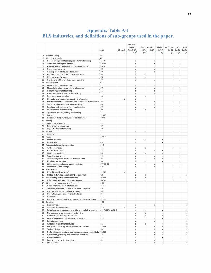
33

Appendix Table A-1 BLS industries, and definitions of sub-groups used in the paper.

NAICS IT‐prod.

Bus, excl. 

Nat Res, 

Con, FIRE

IT‐int. 

(in (2))

Not‐IT‐int. 

(in (2))

Fin‐int.

(in (2))

Not fin. Int

(in (2))

Well

(in (2))

Poor

(in (2))

(1) (2) (3) (4) (5) (6) (7) (8)

1     Manufacturing MN

2     Nondurable goods ND

3       Food, beverage and tobacco product manufacturing 311,312 x x x x

4       Textile and textile product mills 313,314 x x x x

5       Apparel, leather, and allied product manufacturing 315,316 x x x x

6       Paper manufacturing 322 x x x x

7       Printing and related support activities 323 x x x x

8       Petroleum and coal products manufacturing 324 x x x x

9       Chemical manufacturing 325 x x x x

10       Plastics and rubber products manufacturing 326 x x x x

11     Durable goods DM

12       Wood product manufacturing 321 x x x x

13       Nonmetallic mineral product manufacturing 327 x x x x

14       Primary metal manufacturing 331 x x x x

15       Fabricated metal product manufacturing 332 x x x x

16       Machinery manufacturing 333 x x x x

17       Computer and electronic product manufacturing 334 x x

18       Electrical equipment, appliance, and component manufacturing335 x x x x

19       Transportation equipment manufacturing 336 x x x x

20       Furniture and related product manufacturing 337 x x x x

21       Miscellaneous manufacturing 339 x x x x

22     Agriculture, forestry, fishing, and hunting 11

23       Farms 111,112

24       Forestry, fishing, hunting, and related activities 113-115

25     Mining 21

26       Oil and gas extraction 211

27       Mining, except oil and gas 212

28       Support activities for mining 213

29     Utilities 22 x x x x

30       Construction 23

31     Trade 42,44-45

32       Wholesale trade 42 x x x x

33       Retail trade 44,45 x x x x

34     Transportation and warehousing 48-49

35       Air transportation 481 x x x x

36       Rail transportation 482 x x x x

37       Water transportation 483 x x x x

38       Truck transportation 484 x x x x

39       Transit and ground passenger transportation 485 x x x x

40       Pipeline transportation 486 x x x x

41       Other transportation and support activities 487,488,492 x x x x

42       Warehousing and storage 493 x x x x

43     Information 51

44       Publishing (incl. software) 511,516 x x

45       Motion picture and sound recording industries 512 x x x x

46     Broadcasting and telecommunications 515,517 x x x x

47       Information and Data Processing Services  518,519 x x x x

48     Finance, Insurance, and Real Estate  52-53

49       Credit intermed. and related activities 521,522

50       Securities, commods, and other fin. invest. activities 523

51       Insurance carriers and related activities 524

52       Funds, trusts, and other financial vehicles 525

53       Real estate 531

54       Rental and leasing services and lessors of intangible assets 532,533

55     Services 54-81

56       Legal services 5411 x x x x

57       Computer systems design 5415 x x

58       Miscellaneous professional, scientific, and technical services 5412-5414,5416-5419 x x x x

59       Management of companies and enterprises 55 x x x x

60       Administrative and support services 561 x x x x

61       Waste management and remediation services 562 x x x x

62       Education services 61 x x x x

63       Ambulatory health care services 621 x x x x

64       Hospitals and nursing and residential care facilities 622,623 x x x x

65       Social assistance 624 x x x x

66       Performing arts, spectator sports, museums, and related indus711,712 x x x x

67       Amusement, gambling, and recreation industries 713 x x x x

68       Accommodation 721 x x x x

69       Food services and drinking places 722 x x x x

70       Other services 81 x x x x

34

Bibliography

Aaronson, Daniel and Daniel G. Sullivan (2001). “Growth in Worker Quality.” Federal Reserve Bank of Chicago Economic Perspectives, , Vol. 25, 4th Quarter.

Alexopoulos, Michelle and Jon Cohen (2009). “Measuring our Ignorance, One Book at a Time: New Indicators of Technological Change, 1909–1949.” Journal of Monetary Economics, Volume 56, Issue 4, May, Pages 450-470.

Arnold, Robert (2009). “The Challenges of Estimating Potential Output in Real Time.” Federal Reserve Bank of St. Louis Review, July/August 2009, 91(4), pp. 271-90.

Bank of England (2014). “Inflation Report.” February.

Baily, Martin, James Manyika, and Shalabh Gupta (2013). “U.S. Productivity Growth: An Optimistic Perspective.” International Productivity Monitor, vol. 25, pages 3-12, Spring.

Bartel, Ann, Casey Ichniowski, and Kathryn Shaw (2007). “How Does Information Technology Affect Productivity? Plant-Level Comparisons of Product Innovation, Process Improvement, and Worker Skills.” Quarterly Journal of Economics, November: 1721-1758.

Basu, Susanto and John G. Fernald (2002). “Aggregate Productivity and Aggregate Technology.” European Economic Review.

Basu, Susanto and John G. Fernald (2008). “Information and communications technology as a general-purpose technology: evidence from U.S industry data.” Economic Review, Federal Reserve Bank of San Francisco, pages 1-15.

Basu, Susanto and John Fernald (2009). “What Do We Know and Not Know About Potential Output?” St. Louis Fed Review.

Basu, Susanto, John Fernald, Jonas Fisher, and Miles Kimball (2013). “Sector-Specific Technical Change.” Manuscript, Federal Reserve Bank of San Francisco.

Basu, Susanto, John Fernald, and Miles Kimball (2006). “Are Technology Improvements Contractionary?” American Economic Review.

Basu, Susanto, John Fernald, Nicholas Oulton, and Sally Srinivasan (2003). “The Case of the Missing Productivity Growth: Or, Does Information Technology Explain Why Productivity Accelerated in the United States but Not the United Kingdom?” NBER Macroeconomics Annual, 2003.

Bresnahan, T. F., and M. Trajtenberg. (1995). General-purpose technologies:"Engines of growth"? Journal of Econometrics 65(Special Issue, January): 83-108.

Broda, Christian and David E. Weinstein (2006). "Globalization and the Gains from Variety," The Quarterly Journal of Economics, vol. 121(2), pages 541-585, May.

Brynjolfsson, Erik, and L. M. Hitt. (2000). “Beyond computation: Information technology, organizational transformation and business performance.” Journal of Economic Perspectives 14(4):23-48.

Brynjolfsson, Erik, and Andrew McAffee. (2014). The Second Machine Age: Work, Progress, and Prosperity in a Time of Brilliant Technologies. W. W. Norton & Company.

Byrne, David M., Stephen D. Oliner, and Daniel E. Sichel (2013). “Is the Information Technology Revolution Over?” International Productivity Monitor, vol. 25, pages 20-36, Spring.

35

Caballero, Ricardo J and Mohamad L. Hammour (1994). "The Cleansing Effect of Recessions." American Economic Review, vol. 84(5), pages 1350-68, December

Congressional Budget Office (2014a). “The Budget and Economic Outlook: 2014 to 2024.” The Congress of the United States, Congressional Budget Office. February 2014. http://www.cbo.gov/publication/45010.

Congressional Budget Office (2014b). “Revisions to CBO’s Projection of Potential Output Since 2007.” The Congress of the United States, Congressional Budget Office. February 2014. http://www.cbo.gov/publication/45012

Comin, Diego and Mark Gertler (2006). “Medium-Term Business Cycles.” American Economic Review, vol. 96(3), pages 523-551, June.

Corrado, Carol, and Charles Hulten (2013). “Innovation Accounting.” In: Measuring Economic Sustainability and Progress. National Bureau of Economic Research.

Corrado, Carol, Charles Hulten, and Daniel Sichel (2006). “Intangible Capital and Economic Growth.” Review of Income and Wealth, Series 55, No. 3, September 2009

Daly, Mary C., John G. Fernald, Fernanda Nechio, and Oscar Jordà (2014). “Interpreting Deviations from Okun’s Law.” FRBSF Economic Letter, Forthcoming.

David, Paul and Gavin Wright (2003). “General Purpose Technologies and Productivity Surges: Historical Reflections on the Future of the ICT Revolution.” In Paul A. David and Mark Thomas (eds.), The Economic Future in Historical Perspective. Oxford University Press.

Decker, Ryan John Haltiwanger, Ron S Jarmin, and Javier Miranda (2013). “The Secular Decline in Business Dynamism in the U.S.” Manuscript, University of Maryland.

Fatas, Antonio (2002). "The Effects of Business Cycles on Growth." In Economic Growth: Sources, Trends and Cycles, Eds. Norman Loayza and Raimundo Soto. Central Bank of Chile.

Fernald, John G. (1999). "Roads to Prosperity? Assessing the Link between Public Capital and Productivity." American Economic Review, 89(3): 619-638.

Fernald, John G. (2007). “Trend Breaks and Contractionary Technology Improvements.” Journal of Monetary Economics.

Fernald, John G. (2014). “A Quarterly Utilization-Adjusted Series on Total Factor Productivity.” Manuscript, http://www.frbsf.org/economics/economists/jfernald.html. Data supplement at http://www.frbsf.org/economics/economists/jfernald/quarterly_tfp.xls.

Fernald, John and Shanthi Ramnath (2003). “Information Technology and the U.S. Productivity Acceleration.” Chicago Fed Letter, No. 193, September.

Fernald, John, David Thipphavong, and Bharat Trehan (2007) “Will Fast Productivity Growth Persist?” FRBSF Economic Letter 2007-09.

Field, Alexander J. (2003). "The Most Technologically Progressive Decade of the Century." American Economic Review, 93(4): 1399-1413.

Field, Alexander J. (2007). “The Origins of U.S. Total Factor Productivity Growth in the Golden Age.” Cliometrica, 1:63-90.

Fleischman, Charles and John Roberts (2011). "From Many Series, One Cycle: Improved Estimates of the Business Cycle from a Multivariate Unobserved Components Model, " FEDS Working Paper 2011-46.

36

Foster, Lucia, John C. Haltiwanger, and Cornell J. Krizan (2006). "Market Selection, Reallocation, and Restructuring in the U.S. Retail Trade Sector in the 1990s," The Review of Economics and Statistics, vol. 88(4), pages 748-758, November.

Galí, Jordi, Frank Smets, and Rafael Wouters (2012). “Slow Recoveries: A Structural Interpretation.” Manuscript, CREI.

Gordon, Robert J. (1990). The Measurement of Durable Goods Prices, Chicago: University of Chicago Press.

Gordon, Robert J. (2000). Does the "New Economy" Measure up to the Great Inventions of the Past? Journal of Economic Perspectives, vol.4, no.14 (Fall), pp. 49-74.

Gordon, Robert J. (2006). "The Boskin Commission Report: A Retrospective One Decade Later," International Productivity Monitor, vol. 12, pages 7-22, Spring.

Gordon, Robert J. (2014). “The Demise of U.S. Economic Growth: Restatement, Rebuttal, and Reflections.” NBER WP 19895, February.

Greenspan, Alan (2000). “Technology and the economy.” Speech to the Economic Club of New York, New York, New York, January 13.

Greenwood, Jeremy, Zvi Hercowitz, and Per Krusell (1997). "Long-Run Implications of Investment-Specific Technological Change," American Economic Review, vol. 87(3), pages 342-62.

Greenwood, Jeremy and Mehmet Yorukoglu (1997). "1974," Carnegie-Rochester Conference Series on Public Policy, Elsevier, vol. 46(1), pages 49-95, June.

Hall, Robert E. (2014). “Quantifying the Lasting Harm to the U.S. Economy from the Financial Crisis.” Manuscript prepared for NBER Macroeconomics Annual, 2014.

Haltiwanger, John, Ian Hathaway, and Javier Miranda (2014). “Declining Business Dynamism in the U.S. High-Technology Sector.” Manuscript, February 2014.

Hobijn, Bart and Alistair McKay (2007). “Spurious Investment Prices.” Unpublished manuscript, Federal Reserve Bank of San Francisco.

Helpman, Elhanan, ed. (1998). General Purpose Technologies and Economic Growth. Cambridge, MA: MIT Press.

Jones, Charles A. (2002). “Sources of U.S. Economic Growth in a World of Ideas,” American Economic Review, March 2002, 92 (1), 220–239.

Jorgenson, Dale W. (2001). “Information Technology and the U.S. Economy.” American Economic Review, 91, pp. 1–32.

Jorgenson, Dale W., Mun S. Ho, and Jon D. Samuels (2013). “Economic Growth in the Information Age: A Prototype Industry-Level Production Account for the United States, 1947-2010.” Manuscript, Harvard University.

Jorgenson, Dale W., Mun S. Ho, and Kevin J. Stiroh (2008). "A Retrospective Look at the U.S. Productivity Growth Resurgence." Journal of Economic Perspectives, 22(1): 3-24.

Kahn, James A., and Robert W. Rich (2007). “Tracking the New Economy: Using Growth Theory to Detect Changes in Trend Productivity.” Journal of Monetary Economics, Volume 54, Issue 6, September 2007, Pages 1670–1701.

Kahn, James and Robert Rich (2013). “Productivity Model Update.” http://www.newyorkfed.org/research/national_economy/richkahn_prodmod.pdf. (Dec.)

37

Kiley, Michael T., 2013. "Output gaps," Journal of Macroeconomics, Elsevier, vol. 37(C), pages 1-18.

Lazear, Edward P., Kathryn L. Shaw, and Christopher Stanton (2013). “Making Do with Less: Working Harder During Recessions.” NBER Working Paper 19328.

Liu, Zheng, and Pengfei Wang. 2014. "Credit Constraints and Self-Fulfilling Business Cycles." American Economic Journal: Macroeconomics, 6(1): 32-69.

Mian, Atif R. and Amir Sufi (2012). "What explains high unemployment? The aggregate demand channel." NBER Working Papers 17830.

Nakamura, Leonard (1998). “The Retail Revolution and Food-Price Mismeasurement,” Business Review, Federal Reserve Bank of Philadelphia, May/June.

Nalewaik, Jeremy J. (2010). "The Income- and Expenditure-Side Measures of Output Growth," Brookings Papers on Economic Activity, vol. 1, pp. 71-106.

Nordhaus, William D. (2002). "Productivity Growth and the New Economy," Brookings Papers on Economic Activity, Economic Studies Program, The Brookings Institution, vol. 33(2), pages 211-265.

Oliner, Stephen D., Daniel E. Sichel, and Kevin Stiroh (2007). “Explaining a Productive Decade.” Brookings Papers on Economic Activity.

Oulton, Nicholas and María Sebastiá-Barriel (2013). “Effects of Financial Crises on Productivity, Capital and Employment. Paper Prepared for the IARIW-UNSW Conference on “Productivity: Measurement, Drivers and Trends.” Sydney, Australia, November 26-27, 2013.

Pesaran, Hashem, Andreas Pick and Mikhail Pranovich (2013). "Optimal forecasts in the presence of structural breaks." Journal of Econometrics, 177(2) 134-152.

Petrosky-Nadeu, Nicolas (2013). “TFP during a Credit Crunch.” Journal of Economic Theory, 148(3) May 2013.

Reifschneider, Dave, William Wascher, and David Wilcox (2013). “Aggregate Supply in the United States: Recent Developments and Implications for the Conduct of Monetary Policy.” FEDS Working Paper 2013-77.

Saiz, Albert (2010). "The Geographic Determinants of Housing Supply." Quarterly Journal of Economics, 125 (3): 1253-1296.

Syverson, Chad (2013). “Will History Repeat Itself? Comments on ‘Is the Information Technology Revolution Over?’” International Productivity Monitor, vol. 25, pages 37-40, Spring.

Van Reenen, John, Nicholas Bloom, Mirko Draca, Tobias Kretschmer, Raffaella Sadun, Henry Overman, and Mark Schankerman (2010). “The Economic Impact of ICT.” Research report, SMART N. 2007/0020.

Wang, J. Christina, Susanto Basu, and John Fernald (2009). “A General-Equilibrium Asset-Pricing Approach to the Measurement of Nominal and Real Bank Output.” In Price Index Concepts and Measurement, Erwin Diewert, John Greenlees and Charles Hulten, editors.

Williams, John C. (2013). “The Economy and Monetary Policy: Follow the Demand.” Presentation to The Forecasters Club, New York, February 21, 2013.

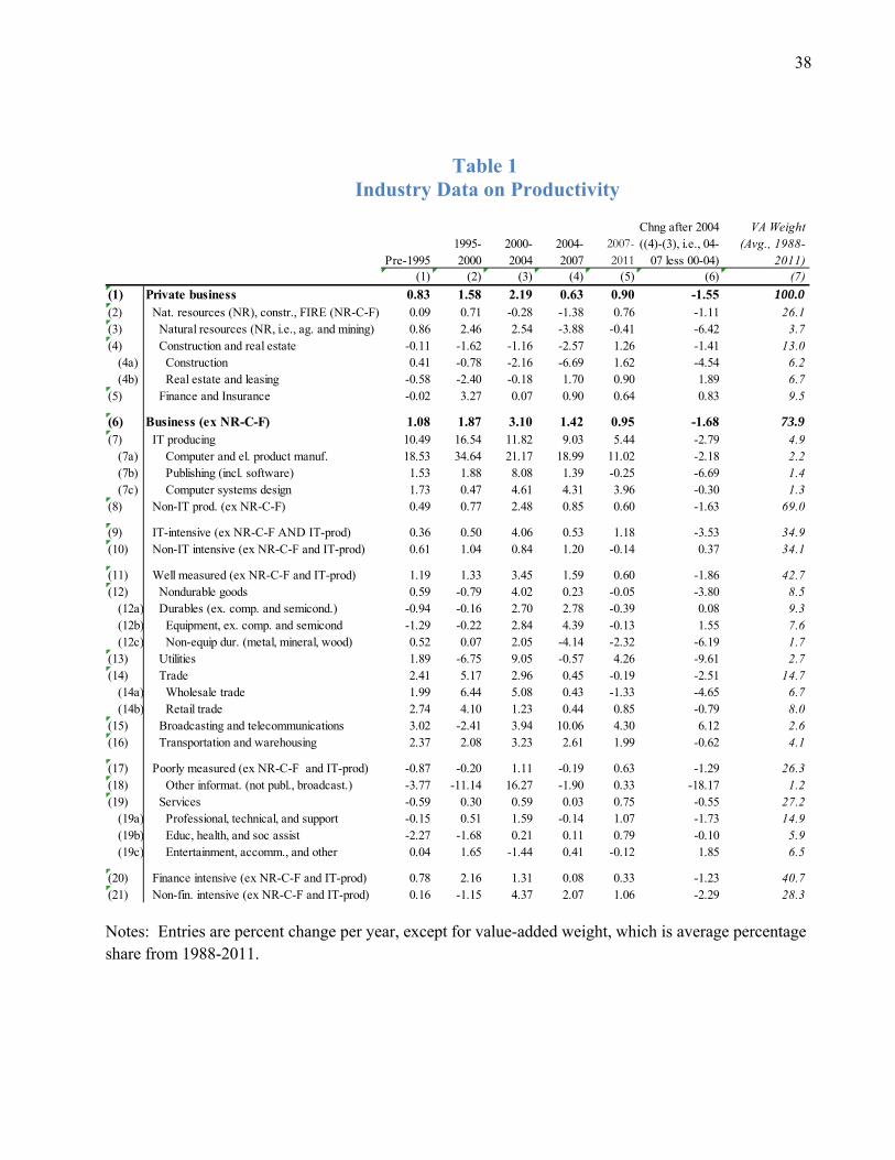
38

Table 1 Industry Data on Productivity

Notes: Entries are percent change per year, except for value-added weight, which is average percentage share from 1988-2011.

Pre-19951995-2000

2000-2004

2004-2007

2007-2011

Chng after 2004 ((4)-(3), i.e., 04-

07 less 00-04)

VA Weight (Avg., 1988-

2011)(1) (2) (3) (4) (5) (6) (7)

(1) Private business 0.83 1.58 2.19 0.63 0.90 -1.55 100.0(2) Nat. resources (NR), constr., FIRE (NR-C-F) 0.09 0.71 -0.28 -1.38 0.76 -1.11 26.1(3) Natural resources (NR, i.e., ag. and mining) 0.86 2.46 2.54 -3.88 -0.41 -6.42 3.7(4) Construction and real estate -0.11 -1.62 -1.16 -2.57 1.26 -1.41 13.0 (4a) Construction 0.41 -0.78 -2.16 -6.69 1.62 -4.54 6.2 (4b) Real estate and leasing -0.58 -2.40 -0.18 1.70 0.90 1.89 6.7(5) Finance and Insurance -0.02 3.27 0.07 0.90 0.64 0.83 9.5

(6) Business (ex NR-C-F) 1.08 1.87 3.10 1.42 0.95 -1.68 73.9(7) IT producing 10.49 16.54 11.82 9.03 5.44 -2.79 4.9 (7a) Computer and el. product manuf. 18.53 34.64 21.17 18.99 11.02 -2.18 2.2 (7b) Publishing (incl. software) 1.53 1.88 8.08 1.39 -0.25 -6.69 1.4 (7c) Computer systems design 1.73 0.47 4.61 4.31 3.96 -0.30 1.3(8) Non-IT prod. (ex NR-C-F) 0.49 0.77 2.48 0.85 0.60 -1.63 69.0

(9) IT-intensive (ex NR-C-F AND IT-prod) 0.36 0.50 4.06 0.53 1.18 -3.53 34.9(10) Non-IT intensive (ex NR-C-F and IT-prod) 0.61 1.04 0.84 1.20 -0.14 0.37 34.1

(11) Well measured (ex NR-C-F and IT-prod) 1.19 1.33 3.45 1.59 0.60 -1.86 42.7(12) Nondurable goods 0.59 -0.79 4.02 0.23 -0.05 -3.80 8.5 (12a) Durables (ex. comp. and semicond.) -0.94 -0.16 2.70 2.78 -0.39 0.08 9.3 (12b) Equipment, ex. comp. and semicond -1.29 -0.22 2.84 4.39 -0.13 1.55 7.6 (12c) Non-equip dur. (metal, mineral, wood) 0.52 0.07 2.05 -4.14 -2.32 -6.19 1.7(13) Utilities 1.89 -6.75 9.05 -0.57 4.26 -9.61 2.7(14) Trade 2.41 5.17 2.96 0.45 -0.19 -2.51 14.7 (14a) Wholesale trade 1.99 6.44 5.08 0.43 -1.33 -4.65 6.7 (14b) Retail trade 2.74 4.10 1.23 0.44 0.85 -0.79 8.0(15) Broadcasting and telecommunications 3.02 -2.41 3.94 10.06 4.30 6.12 2.6(16) Transportation and warehousing 2.37 2.08 3.23 2.61 1.99 -0.62 4.1

(17) Poorly measured (ex NR-C-F and IT-prod) -0.87 -0.20 1.11 -0.19 0.63 -1.29 26.3(18) Other informat. (not publ., broadcast.) -3.77 -11.14 16.27 -1.90 0.33 -18.17 1.2(19) Services -0.59 0.30 0.59 0.03 0.75 -0.55 27.2 (19a) Professional, technical, and support -0.15 0.51 1.59 -0.14 1.07 -1.73 14.9 (19b) Educ, health, and soc assist -2.27 -1.68 0.21 0.11 0.79 -0.10 5.9 (19c) Entertainment, accomm., and other 0.04 1.65 -1.44 0.41 -0.12 1.85 6.5

(20) Finance intensive (ex NR-C-F and IT-prod) 0.78 2.16 1.31 0.08 0.33 -1.23 40.7(21) Non-fin. intensive (ex NR-C-F and IT-prod) 0.16 -1.15 4.37 2.07 1.06 -2.29 28.3

39

Table 2 Number of States with Slowdowns in Labor Productivity Growth

Notes: Table compares growth in GDP per worker before and after 2004 for various industry groupings. For example, column (1) shows the number of states (out of 51, including Washington, D.C.) where average productivity growth from 2004-2007 was slower than from 1997-2004. Industry groupings generally follow Table 1. Columns (2) and (4) show the median slowdown across states, in percentage points at annual rate.

# Slowing 2004-07 fr. 1997-04

Median 04-07 change

# Slowing 2004-12 fr 1997-04

Median 04-12 change

(1) (2) (3) (4)

(1) Private business 47 -1.84 48 -1.44(2) Nat. res. (NR), constr., FIRE (NR-C-F) 48 -2.72 43 -0.99(3) Nat. res. (NR, i.e., ag. and mining) 49 -9.45 49 -6.96(4) Construction 46 -4.63 12 1.33(5) FIRE 43 -1.64 46 -1.52

(6) Private business (ex NR-C-F) 47 -1.36 50 -1.65(7) IT Production 45 -4.94 51 -7.09

(8) Private business (ex NR-C-F and IT prod) 46 -1.11 47 -1.18

(9) IT intensive 50 -1.84 50 -2.12(10) Not-IT intensive 35 -0.56 36 -0.30

(11) Wholesale trade 51 -5.19 51 -5.73(12) Retail trade 49 -2.02 48 -1.33

40

Table 3 Home Prices and State Labor Productivity Slowdowns

 

 

Panel A: ΔLP2004-07 -ΔLP1997-04

Private

Excl. NR-F-C+IT Prod

IT intensive

Not IT intensive Constr FIRE NR

(1) (2) (3) (4) (5) (6) (7) constant -2.06 -1.36 -2.66 -0.61 -4.89 -1.66 -14.50

(0.27) (0.28) (0.33) (0.40) (0.69) (0.53) (2.32)

 

-0.19 0.10 0.36 -0.024 0.08 -0.12 3.16 (0.15) (0.13) (0.13) (0.19) (0.30) (0.28) (1.06)

R2 0.02 0.01 0.05 0.01 0.01 0.02 0.01

 

 

Panel B: ΔLP2005-12 -ΔLP1997-05

Private

Excl. NR-F-C+IT Prod

IT intensive

Not IT intensive Constr FIRE NR

(1) (2) (3) (4) (5) (6) (7) constant -0.71 -1.00 -1.88 -0.28 3.67 -1.18 -1.95

(0.22) (0.20) (0.34) (0.32) (0.54) (0.57) (2.31)

 

0.60 0.15 0.11 0.13 1.38 0.79 2.63 (0.13) (0.11) (0.21) (0.20) (0.33) (0.36) (2.02)

R2 0.14 0.04 0.01 0.18 0.15 0.03 0.01 Notes: Cross-section, population-weighted, IV regressions on 49 U.S. states, including Washington, DC; Hawaii and Alaska are omitted because of missing data. Dependent variable is the change in average productivity for the industry aggregate shown; the top panel looks at 2004-07 from 1997-04; the bottom panel 2005-12 from 1997-05. NR is natural resources, C is construction, F or FIRE is finance, insurance, and real estate. ΔHPI (2001-06) is the change in state home-price indices from 2001Q1 through 2006Q1; ΔHPI (2006-09) is change from 2006:Q1 through 2009:Q2. ΔHPI is normalized by the cross-sectional standard deviation. The Saiz (2010) housing-supply elasticity instruments for the housing-price change.

Indep. var.

Dep var.

ΔHPI (2001‐06) 

Indep. var.

Dep var.

ΔHPI (2006‐09) 

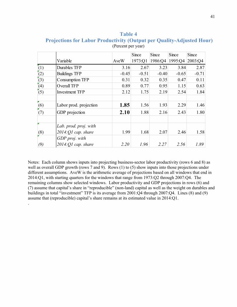
41

Table 4 Projections for Labor Productivity (Output per Quality-Adjusted Hour)

(Percent per year)

Notes: Each column shows inputs into projecting business-sector labor productivity (rows 6 and 8) as well as overall GDP growth (rows 7 and 9). Rows (1) to (5) show inputs into those projections under different assumptions. AveW is the arithmetic average of projections based on all windows that end in 2014:Q1, with starting quarters for the windows that range from 1973:Q2 through 2007:Q4. The remaining columns show selected windows. Labor productivity and GDP projections in rows (6) and (7) assume that capital’s share in “reproducible” (non-land) capital as well as the weight on durables and buildings in total “investment” TFP is its average from 2001:Q4 through 2007:Q4. Lines (8) and (9) assume that (reproducible) capital’s share remains at its estimated value in 2014:Q1. .

Variable AveWSince 1973:Q1

Since 1986:Q4

Since 1995:Q4

Since 2003:Q4

(1) Durables TFP 3.16 2.67 3.23 3.84 2.87(2) Buildings TFP -0.45 -0.51 -0.40 -0.65 -0.71(3) Consumption TFP 0.31 0.32 0.35 0.47 0.11(4) Overall TFP 0.89 0.77 0.95 1.15 0.63(5) Investment TFP 2.12 1.75 2.19 2.54 1.84

(6) Labor prod. projection 1.85 1.56 1.93 2.29 1.46

(7) GDP projection 2.10 1.88 2.16 2.43 1.80

(8)Lab. prod. proj. with 2014:Q1 cap. share 1.99 1.68 2.07 2.46 1.58

(9)GDP proj. with 2014:Q1 cap. share 2.20 1.96 2.27 2.56 1.89

42

Figure 1 Productivity Growth by Sub-Period

43

Figure 2 Potential Output and its Pre-Crisis Trend

Notes: Figure compares actual real GDP to the CBO’s projections for potential prior to the Great Recession (the 2007 line) and CBO’s (2014a) projection, as well as two alternatives that follow the CBO methodology but with different assumptions about utilization. Both alternatives use CBO’s estimated “hours gap” (deviation of hours from steady-state). “Actual TFP” assumes utilization is constant, so that actual TFP measures technology. “Fernald” uses estimated utilization and labor-quality gaps. The “2007” CBO estimates are from January 2008, but are based on data through 2007:Q3. Those estimates have been rescaled to 2009$ so that the 2007 value equals the level in CBO (2014a).

44

Figure 3

Labor productivity since 1973

Source: BLS and Fernald (2014)

.

45

Figure 4 Evolution of Key Growth-Accounting Variables

Notes: Level of utilization is set to zero in 1987:Q4, roughly consistent with the CBO’s estimate that the output gap was close to zero at that point. Source is Fernald (2014).

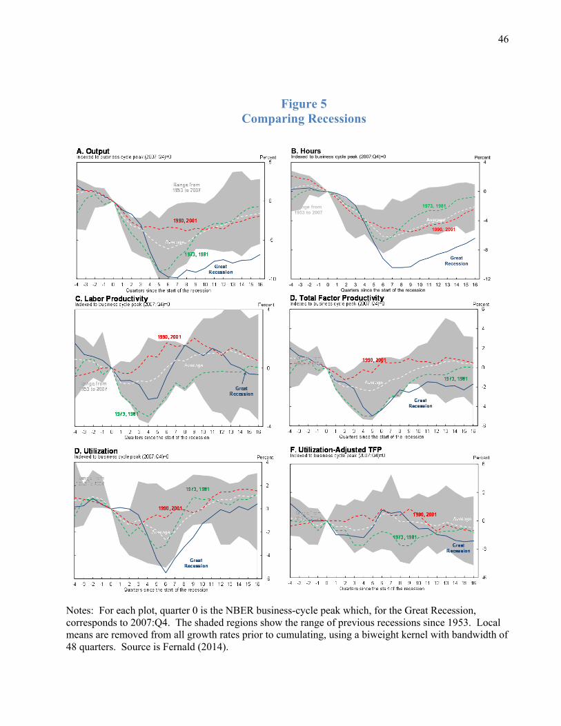
46

Figure 5 Comparing Recessions

Notes: For each plot, quarter 0 is the NBER business-cycle peak which, for the Great Recession, corresponds to 2007:Q4. The shaded regions show the range of previous recessions since 1953. Local means are removed from all growth rates prior to cumulating, using a biweight kernel with bandwidth of 48 quarters. Source is Fernald (2014).

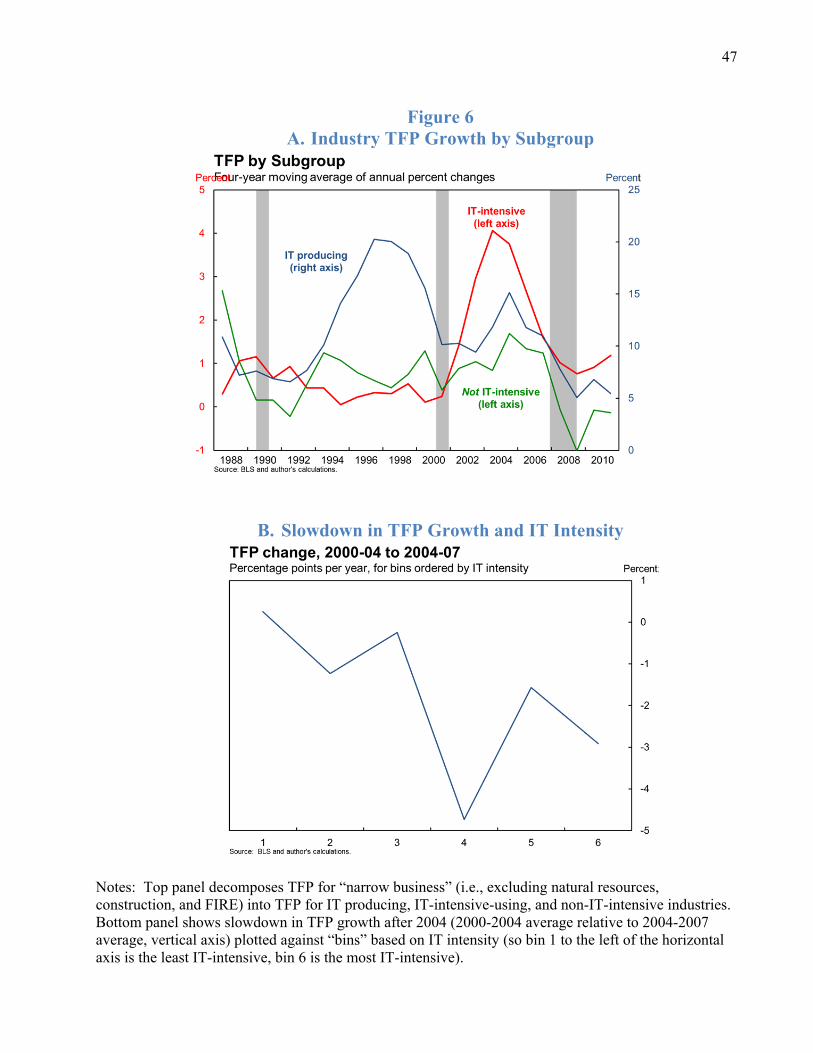
47

Figure 6 A. Industry TFP Growth by Subgroup

B. Slowdown in TFP Growth and IT Intensity

Notes: Top panel decomposes TFP for “narrow business” (i.e., excluding natural resources, construction, and FIRE) into TFP for IT producing, IT-intensive-using, and non-IT-intensive industries. Bottom panel shows slowdown in TFP growth after 2004 (2000-2004 average relative to 2004-2007 average, vertical axis) plotted against “bins” based on IT intensity (so bin 1 to the left of the horizontal axis is the least IT-intensive, bin 6 is the most IT-intensive).

48

Figure 7 TFP by Final Use Sector

49

Figure 8 A. Alternative Utilization Measures

B. CBO and Fernald Estimates of TFP

50

Figure 9 Output Gaps under Different Assumptions

Notes: “Actual TFP” uses the CBO’s (2014a) hours gap but sets the utilization gap to zero. “Fernald” uses the utilization gap estimated in Fernald (2014).