CDE July 2014

PRODUCTION, PROCUREMENT AND INFLATION: A MARKET MODEL FOR FOOD GRAINS

*

Gopakumar K.U. Department of Economics,

Sri Sathya Sai Institute of Higher Learning, Prasanthi Nilayam, Ananthapur Dist,

Andhra Pradesh, 515134.

V. Pandit Email: vnpandit@gmail.com Department of Economics,

Sri Sathya Sai Institute of Higher Learning, Prasanthi Nilayam, Ananthapur Dist,

Andhra Pradesh, 515134.

Working Paper No. 238

Centre for Development Economics Department of Economics, Delhi School of Economics

PRODUCTION, PROCUREMENT AND INFLATION:

A MARKET MODEL FOR FOOD GRAINS*

Gopakumar K.U. and V. Pandit

Department of Economics,

Sri Sathya Sai Institute of Higher Learning,

Prasanthi Nilayam, Ananthapur Dist,

Andhra Pradesh, 515134.

* We are grateful to Professor Mihir Rakshit for some substantive suggestions. An earlier

version of this paper was presented to a seminar organized by the National Council of

Applied Economic Research, New Delhi in July 2013. We thank some of the participants

particularly, Dr. Ganesh Kumar for their useful comments.

ABSTRACT

Rapid rise in the price of food grains and their continued upsurge is a matter of concern for

not only the government and policy makers but also for all concerned with social welfare.

This is particularly so because increased prices of basic food item cause great distress to the

poor sections of the society who have to spend a large part of their income on food. Quite

naturally, understanding the causes of inflation is of high priority for framing the right policy

to tackle the problem needs a clear understanding of the factors that led to the price rise. The

current study tries to examine how prices get determined in Indian food grains market. This

requires a slightly different approach from the conventional demand and supply framework as

government intervenes in the market through open market operations. To this end, we

propose a structural model, explaining the behavior of food grain prices in the India since

1980-81 through 2011-12 incorporating role of government interventions. Our results

confirm that there is strong impact of demand as well as supply side factors. However, when

it comes to controlling of inflation, demand side management turn out to be a highly

significant. Under supply side management, increased capital stock is found to be effective,

as it significantly boosts production and thereby reducing prices and adding to procurement.

Whereas government intervention play a stabilizing role.

Key words: Food grain output, income, money supply, procurement, support prices, capital

stock.

JEL Classification: E31, Q11, Q18.

1

PRODUCTION, PROCUREMENT AND INFLATION:

A MARKET MODEL FOR FOOD GRAINS

1. Introduction

Understandably, inflation is widely seen as a major problem that must be quickly and

effectively dealt with. In particular, it is argued that persistent inflation may destabilize the

process of growth, in general and also have specific and significant adverse welfare

implications. With regard to growth, inflation may be seen to induce a measure of uncertainty

which may cause a dent to the investment process in addition to the impact of higher costs of

borrowing. As far as welfare is concerned much depends on the structure of inflation, because

prices are bound to rise at different rates. In countries like India, where large proportion of its

population is below poverty line, a higher increase in the prices of basic goods has an

excessively adverse impact on the standard of living of the poorer sections of the society.

Moreover, since the increased prices paid by the final consumer are seldom passed on to the

basic producers, who may also belong to the poorer sections of society, the impact is largely

adverse. In any case, many in the poorer sections of the society would be buyers rather than

sellers of these basic goods. Quite likely, the real incomes of the poorer sections would

record a sharp decline than that of more privileged sections. With more than 30% of its

population living in poverty increasing food prices turn out to be particularly serious for

India. This indeed motivates the present exercise.

An in-depth analysis of the policies to control food inflation is of much concern to the

government agencies, the policy makers and professional economists for two main reasons.

Firstly, the solution package is neither obvious nor one way. Attempts to minimize the impact

of higher food prices by subsidizing them or even by meeting the higher domestic demand

through imports are bound to increase public expenditures and result in high import bills

respectively. With fiscal deficit currently above 5% of GDP the situation is particularly

difficult for India. Moreover, high food prices would typically raise wages and material costs

of most industries which in turn mean higher inflation all around. Moreover, use of monetary

policy which may require raising interest rates and reduced money supply may have a

seriously adverse impact on investment. Thus, a wrong diagnosis of the problem and

corresponding policies may have spillover effects on other sectors, leading to macroeconomic

imbalances. Clearly the likely solutions are not straight forward.

2

2. Food Grains Prices: The Overall Movement

The food grain prices started off quite remarkably in the early fifties with a

deflationary phase for five consecutive years starting with 1950-511. For the same

quinquennium, this was accompanied and indeed caused by a significant output growth with

the growth rates in food grain production averaging more than 7 percent. However these

trends in prices as well as output were not sustained thereafter. No wonders that the first five

year plan primarily focused on uplifting the agrarian economy of India. Notably, the then

Prime Minister Pandit Jawaharlal Nehru said “everything else can wait but not agriculture”.

Of the total plan outlay, 31 percent was devoted to the agricultural sector. However, in the

subsequent plans, the importance given to agricultural sector was steadily reduced. As a

result of reduced public investment, besides other factors like adverse weather conditions,

increased pressure on land for non agricultural purposes, increased input prices; food grain

production in the recent decades got more or less stagnated.

However it is quite remarkable that from about 51 million tonnes in 1951-52 the

production of food grains in 2011-12 has increased to 258 million tonnes. But, we also see

that this rate of growth in food grain production was one of increase only at decreasing rate

rather than that of steady growth. The five year average growth rates in production of food

grains declined subsequently from 7.88 percent in 1950-51 through 1954-55 to about 3

percent for the next 15 years; and almost stagnant over 1970-71 through 1974-75. Though the

average growth rates in production picked up in the next ten years, the upward trend was

once again not sustained. In the following years, it again fell consistently registering negative

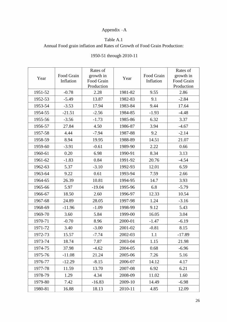
rates of growth during 2000-01 to 2004-05. From Table 1, it is quite clear that for those

periods when a rate of growth in production was low, correspondingly the rate of inflation

was high. This is also important from a welfare point of view because rice, wheat, coarse

cereals, pulses: the major components of the overall food grain basket happen to be the staple

food for majority of Indian population.

In 1956-57 when the food grain production fell by about 7 percent, the prices

immediately shot up at rates above 27 percent. Fortunately for the economy, these explosive

trends eased down quickly and food grain prices were moderate since subsequently. In the

sixties, food grain prices again exploded in 1964-65. Along with modest production, the

Indo-Pak war also had significant impact on the prices this time. No wonder growth rates in

1 For y-o-y annual food grain inflation and growth rates in production see appendix-A

3

grain prices were closer to average of 20 percent for the years 1964-65 through 1967-68. To

add to the problem, 1965-66 the annual rain fall was the lowest since independence till date.

Similar to the sixties, food grain inflation in early 1970‟s also happened to have

similar causes. Initially it was the second Indo-Pak war related to creation of Bangladesh in

1971 that pushed the prices up. However, in the following years, the combined effect of the

international oil shock and deficit monsoon added to the problem by putting further upward

pressure on the prices. In 1971-72 growth rate in production was negative at 3 percent, which

further declined to -7.73 percent the next year. Though production increased marginally in

1973-74, it again fell by 4 percent in 1974-75. Quite naturally in these years we had to import

food grains to meet domestic demand, which further fuelled the domestic prices as food

prices were already high in the international markets. Owing to all these factors, food grain

prices increased rapidly and the rate of increase was closer to 40 percent by 1974-75.

Table: 1

Rates of Inflation and Rates of Growth for Food Grain Production

(Quinquennial Averages)

Period Rates of Inflation in WPI-FG Rates of Growth in Food

Grain Production

1950-51 to 1954-55 -7.83 7.88

1955-56 to 1959-60 6.75 2.83

1960-61 to 1964-65 7.87 3.23

1965-66 to 1969-70 8.20 3.27

1970-71 to 1974-75 15.00 0.30

1975-76 to 1979-80 -0.62 2.86

1980-81 to 1984-85 6.54 6.26

1985-86 to 1989-90 7.24 3.66

1990-91 to 1994 -95 12.67 2.35

1995-96 to 1999-00 9.11 2.01

2000-01 to 2004-05 0.13 -0.18

2005-06 to 2009-10 10.76 2.03

Source: Based on RBI Handbook of Statistics 2010 – 2011 and IEG-DSE Database

During the first half of eighties, grain prices remained quite high at an average closer

to 7 percent despite having excellent crops. In fact growth rate in production of food grains

was above 6 percent which was a rarity barring the early 1950s. However, upward trend in

prices was partly because of the adverse impact of the second oil crisis that could have

fuelled the relative prices. In the latter half of eighties, production was fairly good except for

4

1986-87 and 1987-88. In 1988-89 food grain production marked record production with

increase at 20 percent annually. Quite surprisingly, the prices were also high during this year

having increased at 14 percent. However this could be because of the two consecutive bad

years preceding 1988-89. The next hike in food grain prices was in 1991-92 when prices

increased at 20 percent. Quite surprisingly this was one unique case of food prices going up

rapidly despite good monsoons. During this period it was the cost push factors that were

prominent. Moreover this was the time when economy was getting adjusted to the structural

changes. During this period, as part of new policies, there was huge dose of devaluation

which in turn made the imports costlier. Nevertheless, the overall food grain inflation in the

nineties was quite high with decadal average almost touching 11 percent. On the production

front, the average decadal growth rate in production was just above 2 percent with three years

having negative signs.

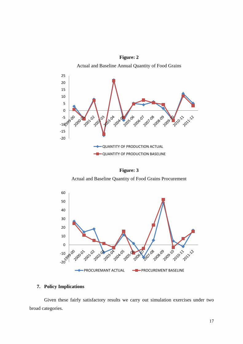
In the first decade of the 21st century, quite contrary to the earlier trends, food grain

inflation was under control despite pitiable output growth. The five year average inflation

during the first half of 2000 was only 0.13 percent. On the other hand, in 2000-01 the food

grain production decreased by 6 percent. This further reduced to -17 percent in 2002-03 and -

4 percent in 2004-05. Year 2003-04 was an exception, as food grain production significantly

increased by 22 percent. In the latter half of the decade 2000-2010 food grain prices increased

even though production was much better than in it‟s the earlier half. This paradoxical trend in

the recent years has gained attention, as many of the academicians and policy makers

consider it as a clear case where the inflation dynamics has undergone a paradigm shift with

prices driven by demand factors and not merely by production trends.

A closer look reveals a more general problem namely, shortage of food supply along

with increasing demand because of increasing incomes, monetary growth, population and

urbanization that has fueled the food inflation in the recent years. The growth rate in GDP

during the post reform period has on an average been of the order of 6.30 percent as

compared to 4.00 percent in the pre reform era. Thus the current episode of inflation needs to

be understood as relating to a period in which the GDP growth has been quite high. The fact

that inequalities in the distribution of income and wealth influence the level and pattern of

inflation also needs to be underlined in understanding inflation as well as the way

government policy may be shaped.

5

While these factors are fairly well understood and widely discussed for a freely

functioning market economy, their specification is relatively harder for a developing

economy where government intervention take different forms in different situations. These

policies are broadly motivated by the desire to ensure that distress of the common people be

minimized. Government interventions in Indian food market are mainly through the Food

Corporation of India (FCI) through which government procures and maintain stocks of food

grains which are released through public distribution system (PDS) and open market

operations2. Keeping in mind the need for a clear understanding of the underlying process we

specify a structural model with a conventional demand-supply framework, but incorporating

government interventions to explain movements in food grain prices. This is important.

3. Major Empirical Approaches.

It is quite common even today for policy makers, commentators and a wider class of

researchers to link inflation prominently to monetary phenomena, even though the

discussions may not be routinely guided by the quantity theory of money or even by the

sophisticated monetarism or the new classical economics. The structuralist view of the

problem does, however, make us look more closely at other factors underlying the price

system even at the macroeconomic level. In an early study Pandit (1978) has highlighted the

role of cost-push factors, which supports structuralist explanation with a considerable

emphasis on the price of food and raw materials originating from the agricultural sector.

Taylor (1983) clearly emphasizes how lagging food supply leads to inflation. For further

insights into the problem at hand, we may also refer to some important studies e.g., Pandit

(1984), Bhujangarao (1987), Sekhar (2003), Gaiha, and Kulkarni (2005) and Kumar and

Sharma (2006).

Studies relating to movements of food prices in India have generally tried to analyze

these under the simple demand supply frame work at equilibrium price and quantities. Many

of these studies3 have used either single equation reduced form framework or partial

adjustment models to explain the inflationary process. This may formally be expressed as:

2 For more detailed discussions on issues regarding government policies and its intervention in food

grain market one may refer to; Rakshit (2001, 2003), Basu (2011), Gupta (2013). 3 See Bhujangarao (1987) for details.

6

P = h [ M, Q, ZPF, P(-1)]

(1)

Where price level P is estimated as a function of money supply M, net availability Q,

and a dummy ZPF to account for other factors. With a year lagged dependent variable as well

as other factors it gives us a dynamic system. The model is basically within the quantity

theory framework with an adaptive expectation formulation, where current/future prices are

estimated as functions of lagged and contemporary prices and money supply. However, such

a specification may not be able to adequately capture the price dynamics in India, especially

that for agricultural/food articles for two reasons. Firstly, quantity cannot be considered

purely exogenous as there can be possibilities of bi-directional causality between prices and

quantities demanded / supplied in the market. Secondly, government intervention in market

plays a crucial role in the market.

Estimating a demand-supply framework at equilibrium price and quantity, can

considerably solve this problem by accounting for interactions between price and quantity

phenomena. Further, the role of government interventions can be brought in either through

demand or supply equations. However, this formulation will require solving the model

simultaneously with appropriate estimation methods4. Alternatively, considering all the

factors that get into each of these equations, a reduced form equation can be estimated either

with prices or quantity as dependent variable. This model can be estimated using OLS

procedure. Such a reduced form specification estimated by Bhujangarao (1987) is as follows.

P = f [C, YLD, SK(-1), PDS, M, GDP, CRAG] (2)

Where, P is price of food grains, which is estimated as function of average costs C,

yield YLD, one year lagged stocks SK(-1), public distribution system PDS, money supply M,

real income GDP, and credit to agriculture CRAG. The above framework was highly relevant

and very well accepted for the estimated sample period till 1983. The analysis confirms the

significance of public distribution system, money supply, input costs and yields in

determining the price movements.

4 It is well known that using OLS procedure to estimate system of equations with variables having bi-

directional causality among the variables can lead to inconsistent results. We may thus have to use

2SLS method of estimation.

7

However, the structure of Indian economy also has changed significantly with

opening up of economy in the early 1990‟s which threw open the economy and, in particular,

the protected agricultural sector for external challenges. Under the open economic framework

fluctuations in the international prices are likely to affect the relative prices in the domestic

economy through exports and imports (Sekhar, 2003, 2011). Though explanation of price

movements under reduced form equations can to an extent be used to bring in the important

variables in consideration under one single equation, the formulation will not allow the model

to effectively capture the dynamics for determining prices and more so for variations in rates

of inflation. Moreover, given the macroeconomic setup, the strong role of structural factors

determining the rates of inflation cannot be sidelined.

A way out to estimate the model clearly lies in the use of a structural model (Pandit,

2000, 2004). The basic aim is to reflect inter-dependence of endogenous variables which are

jointly and simultaneously determined for equilibrium. Exogenous variables can either be

policy instruments or lagged dependent variables or, even natural factors. Estimating

structural model will also have the advantage of specifying separate equations for each of the

endogenous variables rather than bringing them under one reduced form frame work. Studies

by Sekhar (2003) and Kumar and Sharma (2006) have used structural models in modeling

some disaggregate food prices.

Irrespective of the analytical framework or the particular specifications, most of the

studies have identified few common variables that determine food prices. Which includes

production measured in terms of actual production or even net availability, various measures

of income, liquidity and population representing demand variables; various cost push factors

like area of production, fertilizer consumption, agricultural credit, wages etc.; policy

variables such as procurement prices, support prices, government stocks and more

importantly natural factors like rainfall and area cultivated.

4. The Proposed Framework

Keeping the foregoing issues in mind we specify our model as follows. Departing

from the usual procedure of explaining the rate of inflation, we set up two market oriented

relationships – one for the demand and one for the supply. In addition, taking into account the

fact that government intervenes in the market through its procurement policy, under which it

announces the minimum support price and accepts whatever quantity the producers may be

8

willing to offer for procurement. Moreover, government also runs a public distribution

system under which it offers a certain quantity referred to as off-take of food grains, mainly

cereals. This framework gives us a structural model capable of a richer explanation of the

price movements. Before we specify this, let us recapitulate the main features of what one is

trying to capture.

a) Government runs a public distribution system under which it maintains a stock

of food grains acquired by procurement. A certain amount of this quantity is

released in the market every year through PDS.

b) Increase in price of other food articles may tempt people to substitute the

costly food with relatively cheaper grains and this may further increase prices

of food grains. This in short captures the effect of relative prices.

c) Farmers are free to offer part of their production for procurement at the

minimum support price fixed by the government for each product for the year.

Else farmers have an alternative option to sell their produce in the market.

d) The supply is dependent on the capital stock in agriculture, minimum support

prices, area cultivated and the weather conditions, as measured by the annual

rainfall.

e) On the demand side we must include the real disposable income and the

liquidity condition as measured by real money stock.

Variables and the notation used are as follows.

Notation Variable

Q Production of food grains

P WPI for food grains - average for the year

P* WPI for other food articles – average for the year

Y Real Personal Disposable Income

M3 Real money supply (stock at beginning of the year)

PR Procurement of food grains

OT Off-take of food grains through PDS

MSP Minimum support price for food grains

KAG Net capital stock in agriculture at 2004-05 prices.

A Area under cultivation

RF Total annual rainfall

9

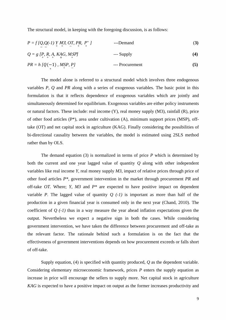
The structural model, in keeping with the foregoing discussion, is as follows:

P = f [Q−

,Q−

(-1) Y+

M3+

, OT−

, PR+

, 𝑃∗

+ ] ---Demand (3)

Q = g [P+

, R+

, A+

, KAG+

, MSP+

] --- Supply (4)

PR = h [𝑄(−1) +

, MSP+

, P−

] --- Procurement (5)

The model alone is referred to a structural model which involves three endogenous

variables P, Q and PR along with a series of exogenous variables. The basic point in this

formulation is that it reflects dependence of exogenous variables which are jointly and

simultaneously determined for equilibrium. Exogenous variables are either policy instruments

or natural factors. These include: real income (Y), real money supply (M3), rainfall (R), price

of other food articles (P*), area under cultivation (A), minimum support prices (MSP), off-

take (OT) and net capital stock in agriculture (KAG). Finally considering the possibilities of

bi-directional causality between the variables, the model is estimated using 2SLS method

rather than by OLS.

The demand equation (3) is normalized in terms of price P which is determined by

both the current and one year lagged value of quantity Q along with other independent

variables like real income Y, real money supply M3, impact of relative prices through price of

other food articles P*, government intervention in the market through procurement PR and

off-take OT. Where; Y, M3 and P* are expected to have positive impact on dependent

variable P. The lagged value of quantity Q (-1) is important as more than half of the

production in a given financial year is consumed only in the next year (Chand, 2010). The

coefficient of Q (-1) thus in a way measure the year ahead inflation expectations given the

output. Nevertheless we expect a negative sign in both the cases. While considering

government intervention, we have taken the difference between procurement and off-take as

the relevant factor. The rationale behind such a formulation is on the fact that the

effectiveness of government interventions depends on how procurement exceeds or falls short

of off-take.

Supply equation, (4) is specified with quantity produced, Q as the dependent variable.

Considering elementary microeconomic framework, prices P enters the supply equation as

increase in price will encourage the sellers to supply more. Net capital stock in agriculture

KAG is expected to have a positive impact on output as the former increases productivity and

10

also gives access to better technology and farm inputs. Government interventions enter the

supply equation through minimum support prices MSP. Once again higher MSP is an

assurance to farmers, which encourage them to produce more. Other variables like rainfall RF

and area cultivated A also enter the supply equation accounting for domestic supply inputs.

Apart from the standard demand-supply framework, an important feature of the model

is the inclusion of equation (5) for procurement PR in which we consider difference of

minimum support prices MSP and prices P as independent variable. This formulation is

indented to take into account dual selling windows available for the sellers5. In other words,

sellers have an option to sell their product to government when MSP is attractive. In an

alternative scenario if MSP is below market price, procurement will be low as suppliers get a

higher price in the local market. However it can also be argued that higher procurement can

lead to increase in prices as it reduces availability in the common market. To this end we

have, accounted for the link from procurement equation to demand equation by taking

difference of procurement to off-take as an independent variable expecting a positive relation

with the dependent variable namely price P. Furthermore, quantity Q enters the procurement

equation with a year lagged value and is expected to have positive impact on the dependent

variable.

The model presented is in keeping with the basic theory involving several

macroeconomic entities and facts on the ground. The purpose is to start with micro theoretic

model which eventually can lead us to explain overall macroeconomic phenomena under

discussion. However, as mentioned earlier, these factors are not independently determined

and have got continuous interactions which make the system rather complex and dynamic.

Since the empirical estimation of such a model using OLS may result in inconsistent

estimates, we have used 2SLS methodology for estimation as stated earlier.

5. Data and Empirical Results

Before going into the estimation of the model and discussion of results we first

present details of the data used for the study. In all the cases data is obtained from the official

published sources or the official websites of the concerned departments. The sample period

for the analysis cover from 1980-81 through 2011-12 and as mentioned earlier, variables are

taken as growth rates. The following table presents information on variables its unit of

5 For further discussions on microeconomic foundations of MSP and its impact on the Indian food

grain market refer to Basu (2011).

11

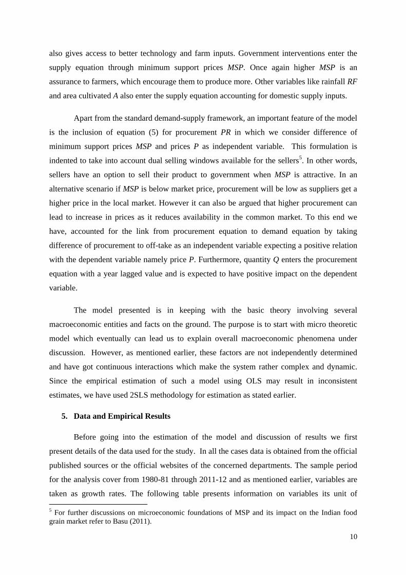
measurements and official sources. However, in the specified model each variable is

measured as percent (y-o-y) rate of growth.

Table: 2

Data and Sources

Data and units Publication Official Sources

Production of food grains

(Million tonnes)

Economic Survey

(2012-13).

Directorate of Economics &

Statistics, Department of Agriculture

& Cooperation.

Wholesale Price Index for

Food grains (2004-05 = 100)

Handbook of Statistics,

Reserve Bank of India.

Office of Economic Advisor,

Ministry of Commerce and Industry.

Whole Price Index for Other

Food Articles (2004-05 = 100)

Handbook of Statistics,

Reserve Bank of India.

Office of Economic Advisor,

Ministry of Commerce and Industry.

Personal Disposable Income

(crores)

Handbook of Statistics,

Reserve Bank of India. Central Statistics Office.

Broad Money Supply (Rupees

billion)

Handbook of Statistics,

Reserve Bank of India. Reserve Bank of India.

Procurement (Million tonnes) Economic Survey

(2012-13)

Ministry of Food, Consumer Affairs

and Public Distribution.

Off-take (Million tonnes) Economic Survey

(2012-13)

Ministry of Food, Consumer Affairs

and Public Distribution.

Minimum Support Prices

(Rupees per quintal)

Handbook of Statistics,

Reserve Bank of India.

1. Ministry of Agriculture.

2. Commission for Agricultural

Costs and Prices. (CACP)

Net Capital Stock (in crores) National Accounts

Statistics.

Central Statistical Organization,

Ministry of Statistics and Programme

Implementation.

Area of production (Million

hectares)

Handbook of Statistics,

Reserve Bank of India. Ministry of Agriculture.

Rainfall (millimeters) Indian Meteorological

Department portal. Ministry of Earth Science.

Price of other food articles is taken as the weighted average of wholesale price index

for fruits, vegetables, milk, egg, meat and fish at 2004-05 prices. Minimum Support Prices

for total food grains is weighted average of MSP for coarse cereals, rice, wheat and pulses;

where the weights are equal to their corresponding weights in the wholesale price index with

2004-05 as base year. Real personal income and real money supply is obtained by deflating

12

the corresponding nominal magnitudes with wholesale price index for all commodities (WPI-

AC) at 2004-05 = 100.

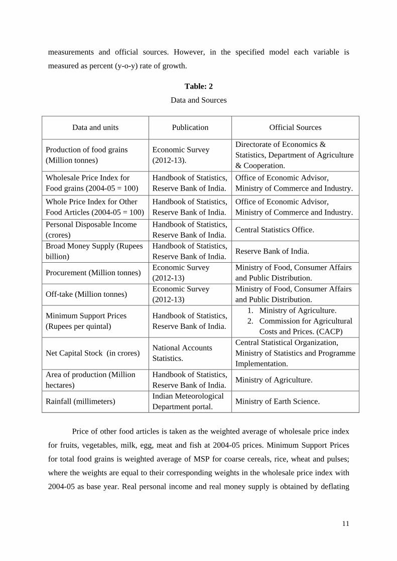
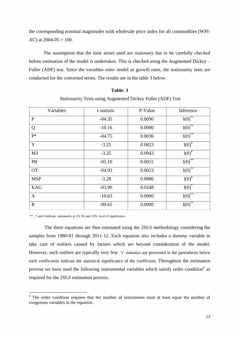
The assumption that the time series used are stationary has to be carefully checked

before estimation of the model is undertaken. This is checked using the Augmented Dickey –

Fuller (ADF) test. Since the variables enter model as growth rates, the stationarity tests are

conducted for the converted series. The results are in the table 3 below.

Table: 3

Stationarity Tests using Augmented Dickey Fuller (ADF) Test

** , * and # indicate stationarity at 1% 5% and 10% level of significance.

The three equations are then estimated using the 2SLS methodology considering the

samples from 1980-81 through 2011-12. Each equation also includes a dummy variable to

take care of outliers caused by factors which are beyond consideration of the model.

However, such outliers are typically very few. „t‟ statistics are presented in the parenthesis below

each coefficients indicate the statistical significance of the coefficient. Throughout the estimation

process we have used the following instrumental variables which satisfy order condition6 as

required for the 2SLS estimation process.

6 The order condition requires that the number of instruments must at least equal the number of

exogenous variables in the equation.

Variables t-statistic P-Value Inference

P -04.35 0.0090 I(0)**

Q -10.16 0.0000 I(0)**

P* -04.75 0.0036 I(0)**

Y -3.25 0.0823 I(0)#

M3 -3.25 0.0943 I(0)#

PR -05.10 0.0015 I(0)**

OT -04.93 0.0023 I(0)**

MSP -3.28 0.0886 I(0)#

KAG -03.90 0.0248 I(0)*

A -10.63 0.0000 I(0)**

R -09.65 0.0000 I(0)**

13

Instruments (exogenous variables) include: P (-1), Q (-1), PR (-1), OT, Y, M3, MSP, KAG,

A, R, DUM1, DUM2, and DUM3.

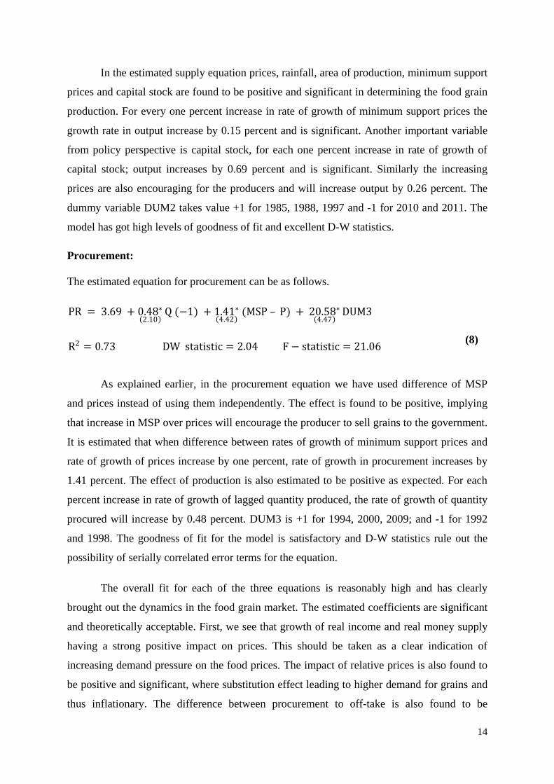
Demand:

To begin with, we estimate the demand equation as follows.

In the demand equation relative prices and income turns out to be a highly significant

factor along with the quantity available, money supply and the PDS. Significant and positive

coefficients for income and money supply indicate increased demand pressure on rate of

growth of food grain prices which is nothing but inflation. For every one percent increase in

rate of growth in income and money supply, food grain inflation, as far as demand is

concerned will increase by 1.16 percent and 0.54 percent respectively. The impact of relative

prices is also positive as expected; for each one percent of increase in rate of inflation for

other food articles, inflation for food grains increase by 0.51 percent. Both the current and

lagged coefficient for production of food grains as expected is having a negative and

significant impact on inflation. For one percent increase in rate of growth of quantity

available, the inflation decreases by 0.38 percent. Whereas the impact of the lagged

coefficient will pull down inflation by 0.34 percent. The difference of procurement and off-

take, as expected is having positive impact on prices and is fairly significant. DUM1 is

assigned a value of +1 for the year 1985 and 2000 and -1 for 1987, 2001, and 2011. The

model has got good fit and DW statistic rules out the possibility of serious auto correlation.

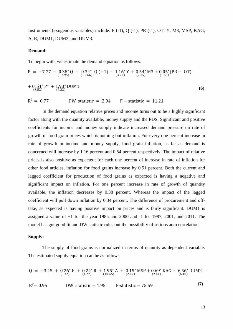
Supply:

The supply of food grains is normalized in terms of quantity as dependent variable.

The estimated supply equation can be as follows.

Q = −3.45 + 0.26∗

3.32 P + 0.24∗

4.27 R + 1.95∗

10.46 A + 0.15∗

2.02 MSP + 0.69∗

2.44 KAG + 6.56∗

6.40 DUM2

R2= 0.95 DW statistic = 1.95 F-statistic = 75.59

(7)

P = −7.77 − 0.38∗

−2.95 Q − 0.34∗

−2.66 Q (−1) + 1.16∗

3.22 Y + 0.54∗

2.15 M3 + 0.05∗

1.66 (PR − OT)

+ 0. 51∗

3.52 P∗ + 1.93∗

7.22 DUM1

R2 = 0.77 DW statistic = 2.04 F − statistic = 11.21

(6)

14

In the estimated supply equation prices, rainfall, area of production, minimum support

prices and capital stock are found to be positive and significant in determining the food grain

production. For every one percent increase in rate of growth of minimum support prices the

growth rate in output increase by 0.15 percent and is significant. Another important variable

from policy perspective is capital stock, for each one percent increase in rate of growth of

capital stock; output increases by 0.69 percent and is significant. Similarly the increasing

prices are also encouraging for the producers and will increase output by 0.26 percent. The

dummy variable DUM2 takes value +1 for 1985, 1988, 1997 and -1 for 2010 and 2011. The

model has got high levels of goodness of fit and excellent D-W statistics.

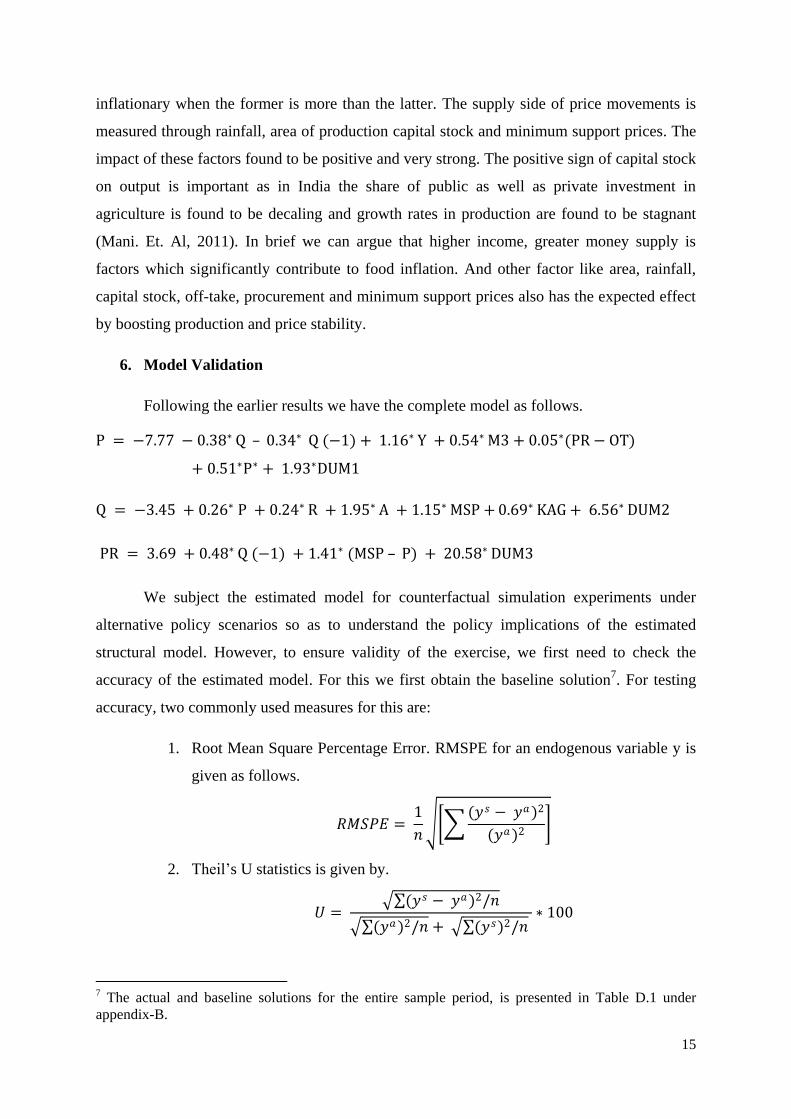
Procurement:

The estimated equation for procurement can be as follows.

As explained earlier, in the procurement equation we have used difference of MSP

and prices instead of using them independently. The effect is found to be positive, implying

that increase in MSP over prices will encourage the producer to sell grains to the government.

It is estimated that when difference between rates of growth of minimum support prices and

rate of growth of prices increase by one percent, rate of growth in procurement increases by

1.41 percent. The effect of production is also estimated to be positive as expected. For each

percent increase in rate of growth of lagged quantity produced, the rate of growth of quantity

procured will increase by 0.48 percent. DUM3 is +1 for 1994, 2000, 2009; and -1 for 1992

and 1998. The goodness of fit for the model is satisfactory and D-W statistics rule out the

possibility of serially correlated error terms for the equation.

The overall fit for each of the three equations is reasonably high and has clearly

brought out the dynamics in the food grain market. The estimated coefficients are significant

and theoretically acceptable. First, we see that growth of real income and real money supply

having a strong positive impact on prices. This should be taken as a clear indication of

increasing demand pressure on the food prices. The impact of relative prices is also found to

be positive and significant, where substitution effect leading to higher demand for grains and

thus inflationary. The difference between procurement to off-take is also found to be

PR = 3.69 + 0.48∗

2.10 Q (−1) + 1.41∗

4.42 (MSP – P) + 20.58∗

4.47 DUM3

R2 = 0.73 DW statistic = 2.04 F − statistic = 21.06

(8)

15

inflationary when the former is more than the latter. The supply side of price movements is

measured through rainfall, area of production capital stock and minimum support prices. The

impact of these factors found to be positive and very strong. The positive sign of capital stock

on output is important as in India the share of public as well as private investment in

agriculture is found to be decaling and growth rates in production are found to be stagnant

(Mani. Et. Al, 2011). In brief we can argue that higher income, greater money supply is

factors which significantly contribute to food inflation. And other factor like area, rainfall,

capital stock, off-take, procurement and minimum support prices also has the expected effect

by boosting production and price stability.

6. Model Validation

Following the earlier results we have the complete model as follows.

P = −7.77 − 0.38∗ Q – 0.34∗ Q (−1) + 1.16∗ Y + 0.54∗ M3 + 0.05∗(PR − OT)

+ 0.51∗P∗ + 1.93∗DUM1

Q = −3.45 + 0.26∗ P + 0.24∗ R + 1.95∗ A + 1.15∗ MSP + 0.69∗ KAG + 6.56∗ DUM2

PR = 3.69 + 0.48∗ Q (−1) + 1.41∗ (MSP – P) + 20.58∗ DUM3

We subject the estimated model for counterfactual simulation experiments under

alternative policy scenarios so as to understand the policy implications of the estimated

structural model. However, to ensure validity of the exercise, we first need to check the

accuracy of the estimated model. For this we first obtain the baseline solution7. For testing

accuracy, two commonly used measures for this are:

1. Root Mean Square Percentage Error. RMSPE for an endogenous variable y is

given as follows.

𝑅𝑀𝑆𝑃𝐸 = 1

𝑛

(𝑦𝑠 − 𝑦𝑎)2

(𝑦𝑎)2

2. Theil‟s U statistics is given by.

𝑈 = (𝑦𝑠 − 𝑦𝑎)2/𝑛

(𝑦𝑎)2/𝑛 + (𝑦𝑠)2/𝑛 ∗ 100

7 The actual and baseline solutions for the entire sample period, is presented in Table D.1 under

appendix-B.

16

Where n is the size of the sample period, ys

and ya

are the forecasted or baseline

solution and actual value of the endogenous variable y. RMSPE and the U are given in Table

4.

Table 4

Model Accuracy: Theil‟s U statistic and RMSPE from 1980-81 through 2011-12

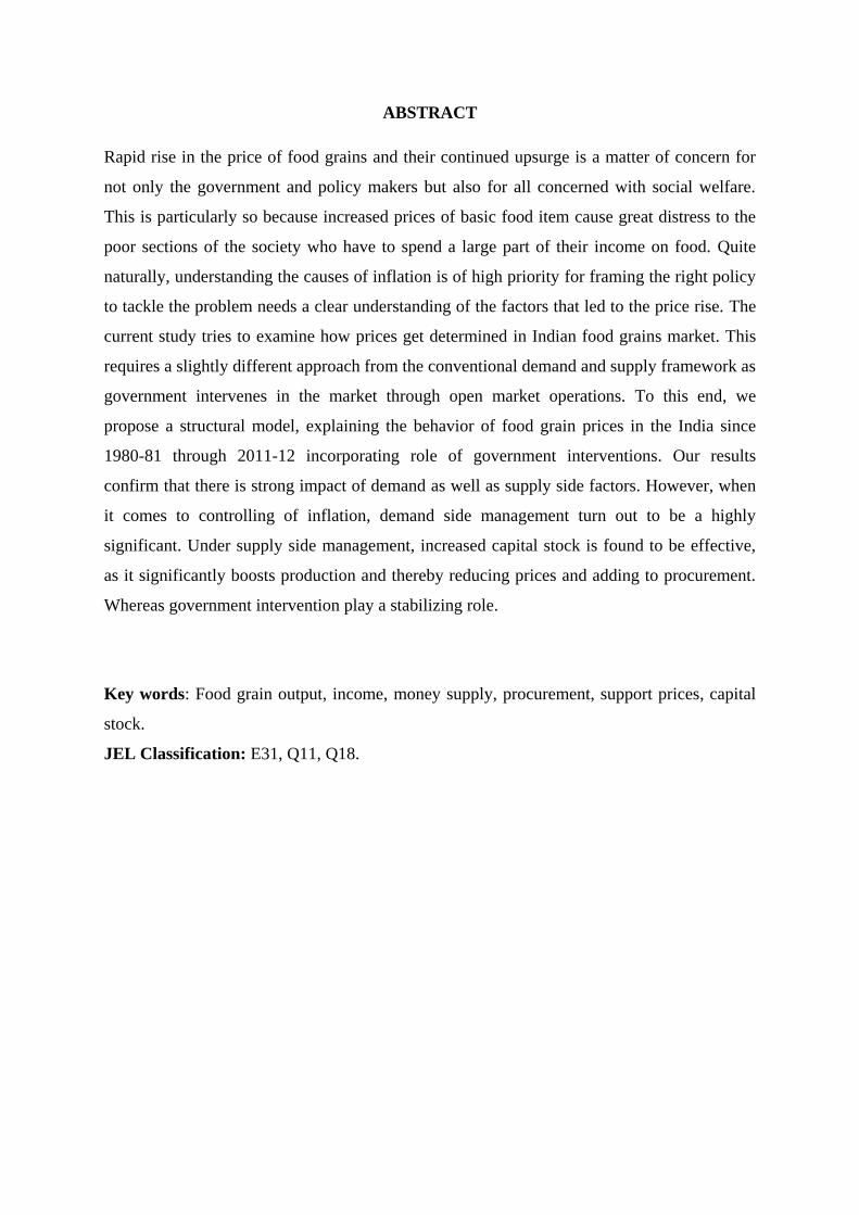
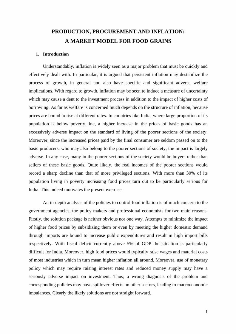
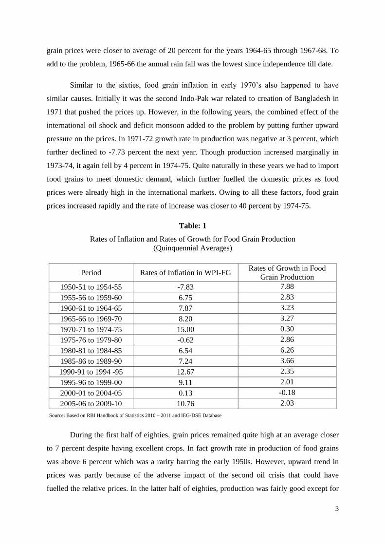
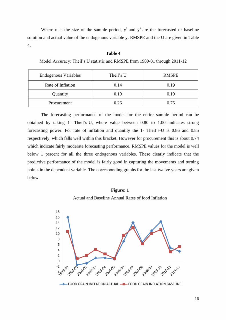
The forecasting performance of the model for the entire sample period can be

obtained by taking 1- Theil‟s-U, where value between 0.80 to 1.00 indicates strong

forecasting power. For rate of inflation and quantity the 1- Theil‟s-U is 0.86 and 0.85

respectively, which falls well within this bracket. However for procurement this is about 0.74

which indicate fairly moderate forecasting performance. RMSPE values for the model is well

below 1 percent for all the three endogenous variables. These clearly indicate that the

predictive performance of the model is fairly good in capturing the movements and turning

points in the dependent variable. The corresponding graphs for the last twelve years are given

below.

Figure: 1

Actual and Baseline Annual Rates of food Inflation

-4

-2

0

2

4

6

8

10

12

14

16

18

FOOD GRAIN INFLATION ACTUAL FOOD GRAIN INFLATION BASELINE

Endogenous Variables Theil‟s U RMSPE

Rate of Inflation 0.14 0.19

Quantity 0.10 0.19

Procurement 0.26 0.75

17

Figure: 2

Actual and Baseline Annual Quantity of Food Grains

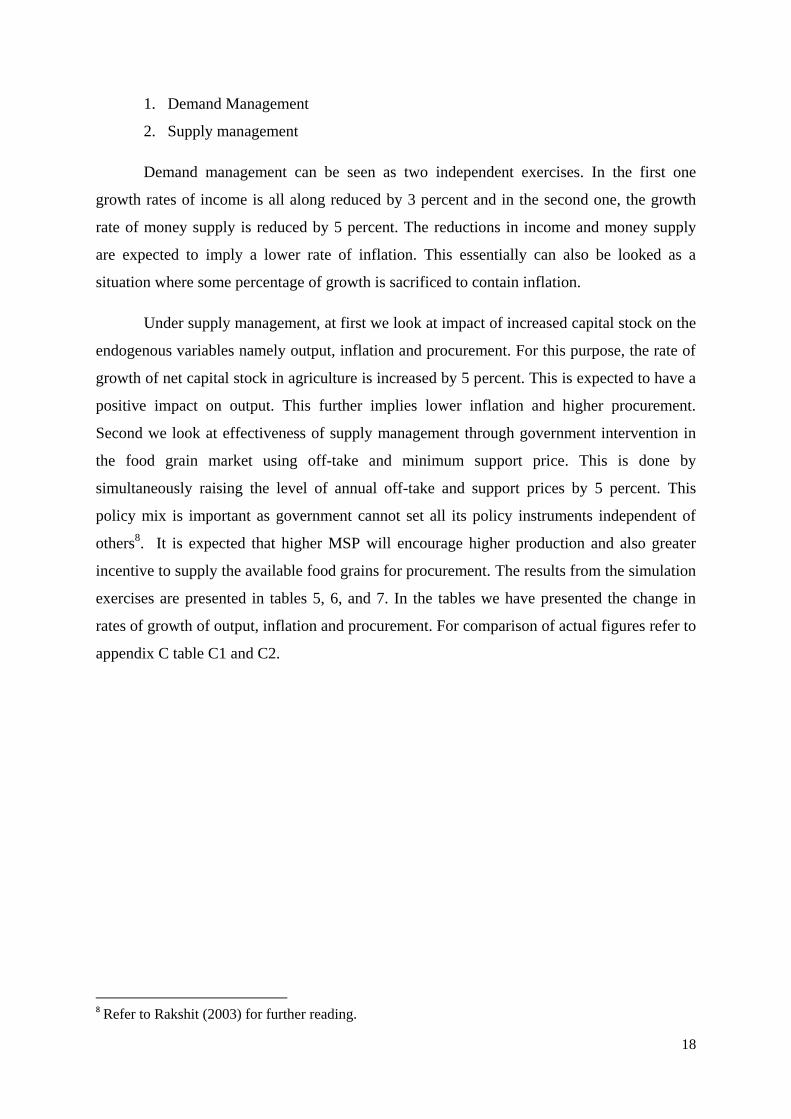
Figure: 3

Actual and Baseline Quantity of Food Grains Procurement

7. Policy Implications

Given these fairly satisfactory results we carry out simulation exercises under two

broad categories.

-20

-15

-10

-5

0

5

10

15

20

25

QUANTITY OF PRODUCTION ACTUAL

QUANTITY OF PRODUCTION BASELINE

-20

-10

0

10

20

30

40

50

60

PROCUREMANT ACTUAL PROCUREMENT BASELINE

18

1. Demand Management

2. Supply management

Demand management can be seen as two independent exercises. In the first one

growth rates of income is all along reduced by 3 percent and in the second one, the growth

rate of money supply is reduced by 5 percent. The reductions in income and money supply

are expected to imply a lower rate of inflation. This essentially can also be looked as a

situation where some percentage of growth is sacrificed to contain inflation.

Under supply management, at first we look at impact of increased capital stock on the

endogenous variables namely output, inflation and procurement. For this purpose, the rate of

growth of net capital stock in agriculture is increased by 5 percent. This is expected to have a

positive impact on output. This further implies lower inflation and higher procurement.

Second we look at effectiveness of supply management through government intervention in

the food grain market using off-take and minimum support price. This is done by

simultaneously raising the level of annual off-take and support prices by 5 percent. This

policy mix is important as government cannot set all its policy instruments independent of

others8. It is expected that higher MSP will encourage higher production and also greater

incentive to supply the available food grains for procurement. The results from the simulation

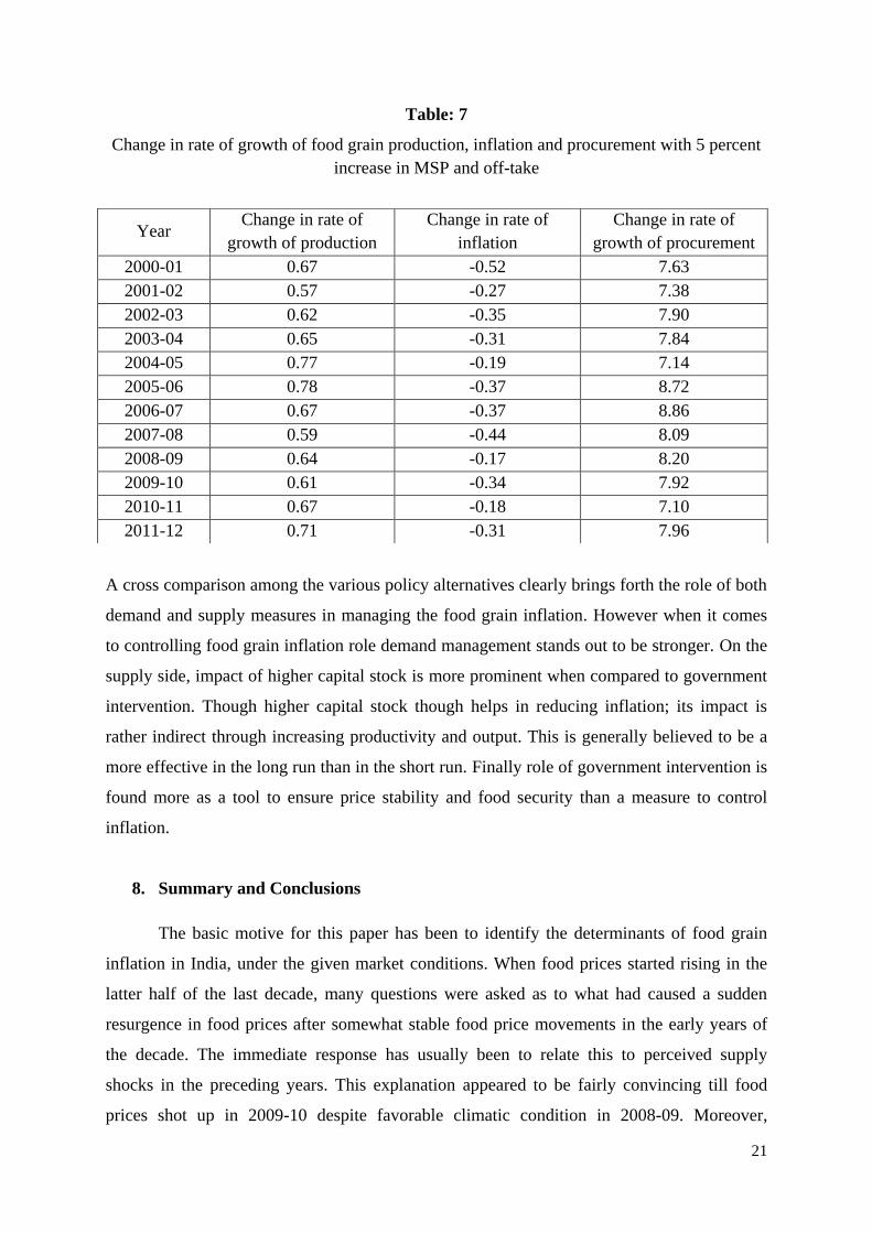
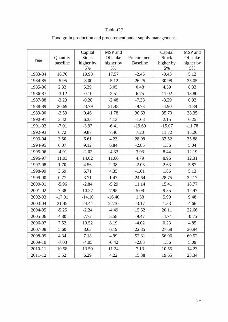
exercises are presented in tables 5, 6, and 7. In the tables we have presented the change in

rates of growth of output, inflation and procurement. For comparison of actual figures refer to

appendix C table C1 and C2.

8 Refer to Rakshit (2003) for further reading.

19

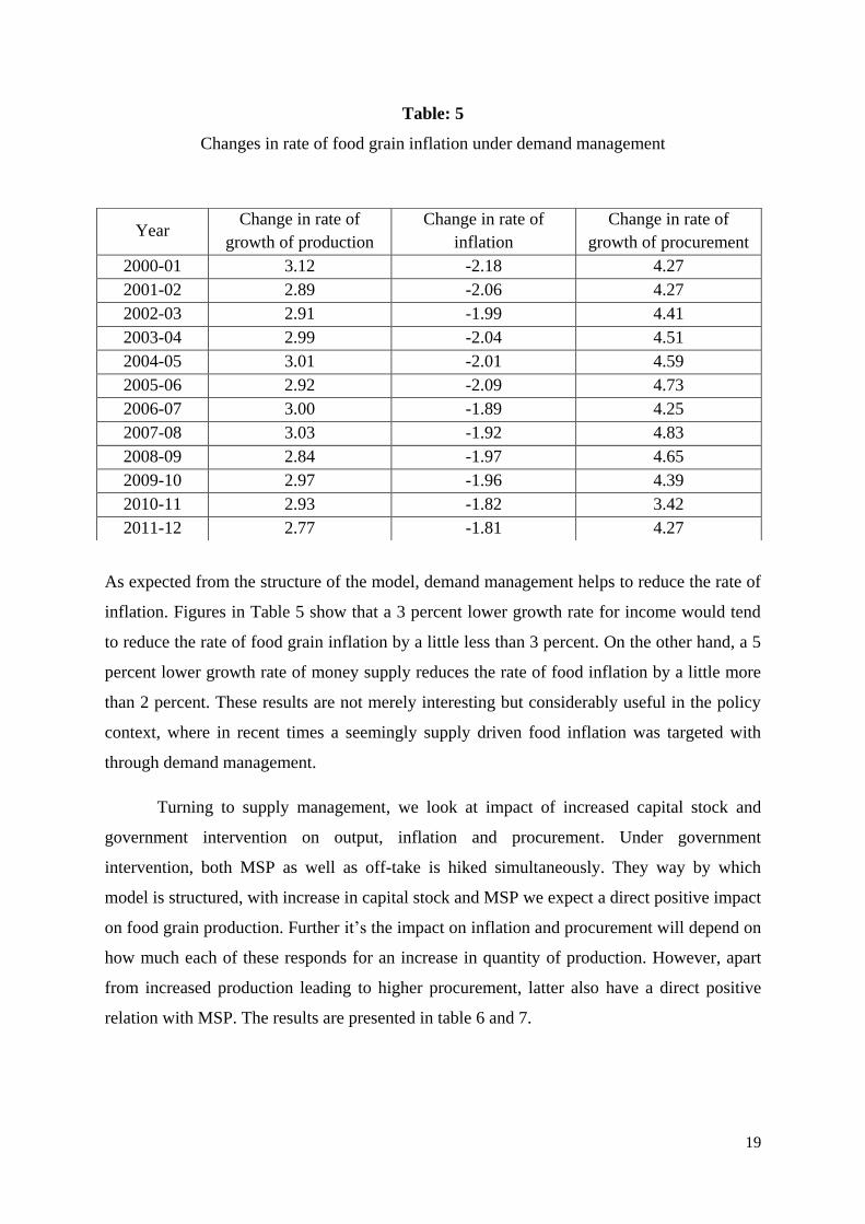
Table: 5

Changes in rate of food grain inflation under demand management

As expected from the structure of the model, demand management helps to reduce the rate of

inflation. Figures in Table 5 show that a 3 percent lower growth rate for income would tend

to reduce the rate of food grain inflation by a little less than 3 percent. On the other hand, a 5

percent lower growth rate of money supply reduces the rate of food inflation by a little more

than 2 percent. These results are not merely interesting but considerably useful in the policy

context, where in recent times a seemingly supply driven food inflation was targeted with

through demand management.

Turning to supply management, we look at impact of increased capital stock and

government intervention on output, inflation and procurement. Under government

intervention, both MSP as well as off-take is hiked simultaneously. They way by which

model is structured, with increase in capital stock and MSP we expect a direct positive impact

on food grain production. Further it‟s the impact on inflation and procurement will depend on

how much each of these responds for an increase in quantity of production. However, apart

from increased production leading to higher procurement, latter also have a direct positive

relation with MSP. The results are presented in table 6 and 7.

Year Change in rate of

growth of production

Change in rate of

inflation

Change in rate of

growth of procurement

2000-01 3.12 -2.18 4.27

2001-02 2.89 -2.06 4.27

2002-03 2.91 -1.99 4.41

2003-04 2.99 -2.04 4.51

2004-05 3.01 -2.01 4.59

2005-06 2.92 -2.09 4.73

2006-07 3.00 -1.89 4.25

2007-08 3.03 -1.92 4.83

2008-09 2.84 -1.97 4.65

2009-10 2.97 -1.96 4.39

2010-11 2.93 -1.82 3.42

2011-12 2.77 -1.81 4.27

20

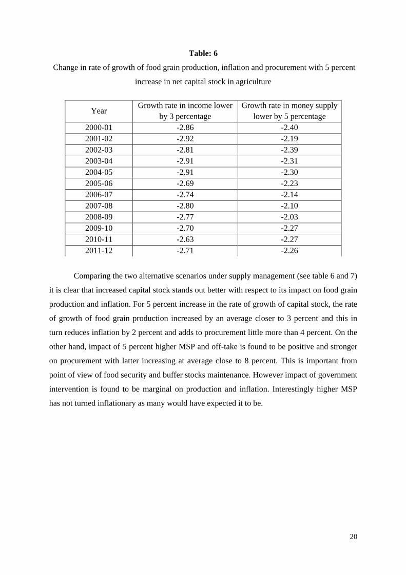
Table: 6

Change in rate of growth of food grain production, inflation and procurement with 5 percent

increase in net capital stock in agriculture

Comparing the two alternative scenarios under supply management (see table 6 and 7)

it is clear that increased capital stock stands out better with respect to its impact on food grain

production and inflation. For 5 percent increase in the rate of growth of capital stock, the rate

of growth of food grain production increased by an average closer to 3 percent and this in

turn reduces inflation by 2 percent and adds to procurement little more than 4 percent. On the

other hand, impact of 5 percent higher MSP and off-take is found to be positive and stronger

on procurement with latter increasing at average close to 8 percent. This is important from

point of view of food security and buffer stocks maintenance. However impact of government

intervention is found to be marginal on production and inflation. Interestingly higher MSP

has not turned inflationary as many would have expected it to be.

Year Growth rate in income lower

by 3 percentage

Growth rate in money supply

lower by 5 percentage

2000-01 -2.86 -2.40

2001-02 -2.92 -2.19

2002-03 -2.81 -2.39

2003-04 -2.91 -2.31

2004-05 -2.91 -2.30

2005-06 -2.69 -2.23

2006-07 -2.74 -2.14

2007-08 -2.80 -2.10

2008-09 -2.77 -2.03

2009-10 -2.70 -2.27

2010-11 -2.63 -2.27

2011-12 -2.71 -2.26

21

Table: 7

Change in rate of growth of food grain production, inflation and procurement with 5 percent

increase in MSP and off-take

A cross comparison among the various policy alternatives clearly brings forth the role of both

demand and supply measures in managing the food grain inflation. However when it comes

to controlling food grain inflation role demand management stands out to be stronger. On the

supply side, impact of higher capital stock is more prominent when compared to government

intervention. Though higher capital stock though helps in reducing inflation; its impact is

rather indirect through increasing productivity and output. This is generally believed to be a

more effective in the long run than in the short run. Finally role of government intervention is

found more as a tool to ensure price stability and food security than a measure to control

inflation.

8. Summary and Conclusions

The basic motive for this paper has been to identify the determinants of food grain

inflation in India, under the given market conditions. When food prices started rising in the

latter half of the last decade, many questions were asked as to what had caused a sudden

resurgence in food prices after somewhat stable food price movements in the early years of

the decade. The immediate response has usually been to relate this to perceived supply

shocks in the preceding years. This explanation appeared to be fairly convincing till food

prices shot up in 2009-10 despite favorable climatic condition in 2008-09. Moreover,

Year Change in rate of

growth of production

Change in rate of

inflation

Change in rate of

growth of procurement

2000-01 0.67 -0.52 7.63

2001-02 0.57 -0.27 7.38

2002-03 0.62 -0.35 7.90

2003-04 0.65 -0.31 7.84

2004-05 0.77 -0.19 7.14

2005-06 0.78 -0.37 8.72

2006-07 0.67 -0.37 8.86

2007-08 0.59 -0.44 8.09

2008-09 0.64 -0.17 8.20

2009-10 0.61 -0.34 7.92

2010-11 0.67 -0.18 7.10

2011-12 0.71 -0.31 7.96

22

government policies and market interventions didn‟t seem to produce expected results as

prices continued to increase. This in turn has motivated us to analyze the problem in a larger

context. In particular, we have attempted to incorporate government intervention in the food

grain market.

To this end we have specified a structural model constituting of three equations

relating demand, supply and procurement. The model is estimated using the 2SLS procedure

covering the sample period, 1980-81 through 2011-12. The results do confirm the strong and

significant impact of demand as well as supply factors determining the food grain prices. On

the demand side it is income, money supply and relative prices that turn out to be important

whereas the significant supply factors are rainfall, area cultivated, capital stock and the nature

and extent of government intervention. With regard to this we have specifically looked at the

impact of MSP, procurement and off-take on the prices. The results are again significant as

we find that larger off-take with higher incentives for procurement has a desirable effect.

Since the model has an excellent measure of accuracy, it is legitimate to work out

policy implications with confidence. The model is solved under two alternative policy

scenarios. First, demand management (a) by reducing the rate of growth of income by 3

percent (b) by lowering rate of growth of money supply by 5 percent. Second, supply

management (a) by increasing rate of growth of capital stock by 5 percent (b) through

government interventions in market by increasing off-take and MSP by 5 percent.

The simulation exercises confirm the substantial role of tighter demand conditions in

controlling the increase in prices, where the impact of income is found to be stronger than

that of money supply. Under supply side management, the impact of higher capital stock is

found to have strong and positive impact on production and thereby bringing down inflation

and also adding to procurement. However, increased MSP and off-take turns out to be more

effective as a stabilizing package by improving output as well as procurement. Where the

effect on latter is found to be more strong. As mentioned earlier, this is important to ensure

food security during the hard times. An important point to be noted here is that, for

government policies to bring out the desired changes it is essential to have the right policy

mix as highlighted by Rakshit (2003).

In conclusion, the current exercise clearly brings forth the role of demand and supply

factors along with the government interventions in determining food grain prices. However,

to have a complete understanding of the dynamics involved, it is important to study the

23

problem at a disaggregate level separately for each of the grains. Moreover, the problem of

income and distributive inequalities also needs to be brought in, to have a complete analytical

framework with more realistic policy implications. It is our intuition that income in the model

is in fact a proxy for its increasingly inequitous distribution rather than its overall level. A

formal testing of this “intuition” is, however, not possible because of data problems.

***********

24

REFERENCES

Basu, Kaushik, 2011. India‟s Foodgrains Policy: An Economic Theory Perspective.

Economic and Political Weekly. vol. 46, 37-46.

Bhujangarao, C., 1987. Determinants of Foodgrain Prices in India: An Empirical

Study, 1961-83. Indian Economic Review. vol. 22, 51-77.

Chand, R., 2010. “Understanding the Nature and Cause of Inflation”. Economic and

Political Weekly. Vol. 45, 10-13.

Gaiha, Raghav.,Vani, S. Kulkarni, 2005. Foodgrains Surpluses, Yields and Prices in

India. Global Forum on Agriculture: Policy Coherence for Development, 30th

November-1stDecember 2005. Paris. France.

Gupta, Neha, 2013. Government Intervention In Grain Markets In India: Rethinking

The Procurement Policy. Working Paper NO. 231, Centre for Development

Economics, Delhi School of Economics.

Mani, Harish.et al, 2011. Public Investment in Agricultural and GDP Growth:

Another Look at the Inter Sectoral Linkages and Policy Implications. Working Paper

NO. 201, Centre for Development Economics, Delhi School of Economics.

Pandit, V., 1978. An analysis of Inflation in India, 1950-1975. Indian Economic

Review, Vol.23, No.2.

Pandit, V., 1984. Macroeconomic Adjustments in a Developing Economy: A Medium

Term Model of Outputs and Prices in India. Indian Economic Review, Vol.19, No.1.

Pandit, V., 2000. Macroeconometric Policy Modeling for India: A Review of Some

Analytical Issues. Journal of Quantitative Economics. Vol. 15, 9-24.

Pandit, V., 2004. Economy-wide Structural Modelling: The Changing Perspectives, in

Pandit. V., and K. Krishnamurti, (eds.), Economic Policy Modelling for India,

Oxford University Press, New Delhi.

25

Parmod Kumar., Anil Sharma, 2006. Price Variability and its Determinants: An

Analysis of Major Foodgrains in India. Indian Economic Review, Vol. 41, 149-172.

Rakshit, M., 2001. Some Public Economics of Food Subsidy and Buffer Stock

Operations in India: Part-1. Money and Finance, Jan-June, 90-124.

Rakshit, M., 2003. Food Policy in India: Some Long Term Issues. Economic and

Political Weekely. Vol. 38.

Sekhar, C.S.C., 2003. Determinants of Price in the World Wheat Markets – Hidden

Lessons for Indian Policy Makers?.Indian economic Review. Vol. 38, 167-188.

Sekhar, C.S.C., 2011. World food grain prices – Effect of Exporting Countries‟

Policies. Indian economic Review. Vol. 46, 217-242.

Taylor, Lance, 1983. Structuralist Macroeconomics: Applicable Models for the

Third World, Basic Books, New York.

26

Appendix –A

Table A.1

Annual Food grain inflation and Rates of Growth of Food Grain Production:

1950-51 through 2010-11

Year Food Grain

Inflation

Rates of

growth in

Food Grain

Production

Year Food Grain

Inflation

Rates of

growth in

Food Grain

Production

1951-52 -0.78 2.28 1981-82 9.55 2.86

1952-53 -5.49 13.87 1982-83 9.1 -2.84

1953-54 -3.53 17.94 1983-84 9.44 17.64

1954-55 -21.51 -2.56 1984-85 -1.93 -4.48

1955-56 -3.56 -1.73 1985-86 6.32 3.37

1956-57 27.84 4.50 1986-87 3.94 -4.67

1957-58 4.44 -7.94 1987-88 9.2 -2.14

1958-59 8.94 19.95 1988-89 14.51 21.07

1959-60 -3.91 -0.61 1989-90 2.22 0.66

1960-61 0.20 6.98 1990-91 8.34 3.13

1961-62 -1.83 0.84 1991-92 20.76 -4.54

1962-63 5.37 -3.10 1992-93 12.01 6.59

1963-64 9.22 0.61 1993-94 7.59 2.66

1964-65 26.39 10.81 1994-95 14.7 3.93

1965-66 5.97 -19.04 1995-96 6.8 -5.79

1966-67 18.50 2.60 1996-97 12.33 10.54

1967-68 24.89 28.05 1997-98 1.24 -3.16

1968-69 -11.96 -1.09 1998-99 9.12 5.43

1969-70 3.60 5.84 1999-00 16.05 3.04

1970-71 -0.70 8.96 2000-01 -1.47 -6.19

1971-72 3.40 -3.00 2001-02 -0.81 8.15

1972-73 15.57 -7.74 2002-03 1.1 -17.89

1973-74 18.74 7.87 2003-04 1.15 21.98

1974-75 37.98 -4.62 2004-05 0.68 -6.96

1975-76 -11.08 21.24 2005-06 7.26 5.16

1976-77 -12.29 -8.15 2006-07 14.12 4.17

1977-78 11.59 13.70 2007-08 6.92 6.21

1978-79 1.29 4.34 2008-09 11.02 1.60

1979-80 7.42 -16.83 2009-10 14.49 -6.98

1980-81 16.88 18.13 2010-11 4.85 12.09

27

Appendix - B

Solutions from the model

Table-B.1

Actual and Baseline values for the endogenous variables in the model.

Year Inflation

Actual

Inflation

Baseline

Quantity

Actual

Quantity

Baseline

Procurement

Actual

Procurement

Baseline

1983-84 9.36 8.68 17.64 16.76 6.87 -2.45

1984-85 -1.90 -4.78 -4.48 -5.95 20.48 26.25

1985-86 6.32 3.67 3.37 2.32 4.45 0.48

1986-87 3.96 2.15 -4.67 -3.12 -0.35 6.75

1987-88 9.17 9.63 -2.14 -3.23 -25.03 -7.38

1988-89 14.49 15.18 21.07 20.69 -5.03 -9.73

1989-90 2.27 4.80 0.66 -2.53 42.34 30.63

1990-91 8.31 11.95 3.13 3.42 18.94 -1.68

1991-92 20.77 18.96 -4.54 -7.01 -28.47 -19.69

1992-93 12.00 12.78 6.59 6.72 11.31 7.20

1993-94 7.58 9.97 2.66 3.50 38.22 28.09

1994-95 14.70 13.33 3.93 6.07 -5.34 -2.85

1995-96 6.80 7.64 -5.79 -4.91 -11.32 3.93

1996-97 12.33 8.08 10.54 11.03 -9.57 4.79

1997-98 1.24 2.70 -3.16 1.70 18.96 -2.03

1998-99 9.12 11.66 5.43 3.69 1.51 -1.61

1999-00 16.05 10.89 3.04 0.77 27.11 24.64

2000-01 -1.47 0.79 -6.19 -5.96 14.73 11.14

2001-02 -0.81 2.05 8.15 7.38 18.31 5.08

2002-03 1.10 4.18 -17.89 -17.01 -8.91 1.58

2003-04 1.15 2.56 21.98 21.45 -3.81 -3.17

2004-05 0.68 0.95 -6.96 -5.25 11.62 15.52

2005-06 7.26 9.36 5.16 4.80 1.59 -9.47

2006-07 14.12 12.22 4.17 7.52 -14.34 -4.02

2007-08 6.92 6.29 6.21 5.60 5.32 22.85

2008-09 11.02 10.03 1.60 4.34 48.40 52.31

2009-10 14.49 11.55 -6.98 -7.03 4.41 -2.83

2010-11 4.85 3.37 12.23 10.58 -2.05 7.13

2011-12 3.61 5.23 5.17 3.52 16.83 15.38

28

Appendix - C

Growth rates in production, inflation and procurement under alternative scenarios

Table-C.1

Food grain inflation under demand and supply management.

Year Baseline

Inflation

Income

lower by 3%

Money

Supply lower

by 5%

Capital Stock

higher by 5%

MSP and

Off-take

higher by 5%

1983-84 8.68 5.64 6.13 7.31 8.51

1984-85 -4.78 -7.61 -6.97 -6.97 -5.24

1985-86 3.67 0.58 1.44 1.44 3.13

1986-87 2.15 -0.75 -0.04 -0.01 1.85

1987-88 9.63 6.82 7.36 7.52 9.28

1988-89 15.18 12.39 13.07 13.21 14.89

1989-90 4.80 1.99 2.68 2.76 4.43

1990-91 11.95 9.26 9.95 10.04 11.43

1991-92 18.96 16.28 16.81 16.98 18.52

1992-93 12.78 9.86 10.55 10.67 12.37

1993-94 9.97 7.30 7.99 8.09 9.61

1994-95 13.33 10.56 11.09 11.29 12.96

1995-96 7.64 4.74 5.65 5.63 7.29

1996-97 8.08 5.38 5.99 6.26 7.87

1997-98 2.70 -0.07 0.48 0.74 2.32

1998-99 11.66 9.17 9.73 9.83 11.52

1999-00 10.89 7.92 8.61 8.79 10.43

2000-01 0.79 -2.07 -1.61 -1.39 0.26

2001-02 2.05 -0.87 -0.14 -0.01 1.78

2002-03 4.18 1.37 1.80 2.19 3.83

2003-04 2.56 -0.35 0.25 0.53 2.25

2004-05 0.95 -1.96 -1.35 -1.06 0.76

2005-06 9.36 6.67 7.13 7.27 8.98

2006-07 12.22 9.48 10.08 10.34 11.85

2007-08 6.29 3.49 4.18 4.37 5.85

2008-09 10.03 7.27 8.01 8.06 9.86

2009-10 11.55 8.85 9.28 9.59 11.21

2010-11 3.37 0.74 1.11 1.56 3.19

2011-12 5.23 2.52 2.97 3.42 4.92

29

Table-C.2

Food grain production and procurement under supply management.

Year Quantity

baseline

Capital

Stock

higher by

5%

MSP and

Off-take

higher by

5%

Procurement

Baseline

Capital

Stock

higher by

5%

MSP and

Off-take

higher by

5%

1983-84 16.76 19.98 17.57 -2.45 -0.43 5.12

1984-85 -5.95 -3.00 -5.12 26.25 30.98 35.05

1985-86 2.32 5.39 3.05 0.48 4.59 8.33

1986-87 -3.12 -0.10 -2.51 6.75 11.02 13.80

1987-88 -3.23 -0.28 -2.48 -7.38 -3.29 0.92

1988-89 20.69 23.79 21.48 -9.73 -4.90 -1.89

1989-90 -2.53 0.46 -1.78 30.63 35.70 38.35

1990-91 3.42 6.33 4.13 -1.68 2.15 6.25

1991-92 -7.01 -3.97 -6.41 -19.69 -15.07 -11.78

1992-93 6.72 9.87 7.40 7.20 11.72 15.26

1993-94 3.50 6.61 4.23 28.09 32.52 35.88

1994-95 6.07 9.12 6.84 -2.85 1.36 5.04

1995-96 -4.91 -2.02 -4.33 3.93 8.44 12.19

1996-97 11.03 14.02 11.66 4.79 8.96 12.31

1997-98 1.70 4.56 2.38 -2.03 2.63 5.87

1998-99 3.69 6.71 4.35 -1.61 1.86 5.13

1999-00 0.77 3.71 1.47 24.64 28.75 32.17

2000-01 -5.96 -2.84 -5.29 11.14 15.41 18.77

2001-02 7.38 10.27 7.95 5.08 9.35 12.47

2002-03 -17.01 -14.10 -16.40 1.58 5.99 9.48

2003-04 21.45 24.44 22.10 -3.17 1.33 4.66

2004-05 -5.25 -2.24 -4.49 15.52 20.11 22.66

2005-06 4.80 7.72 5.58 -9.47 -4.74 -0.75

2006-07 7.52 10.52 8.19 -4.02 0.23 4.85

2007-08 5.60 8.63 6.19 22.85 27.68 30.94

2008-09 4.34 7.18 4.99 52.31 56.96 60.52

2009-10 -7.03 -4.05 -6.42 -2.83 1.56 5.09

2010-11 10.58 13.50 11.24 7.13 10.55 14.23

2011-12 3.52 6.29 4.22 15.38 19.65 23.34