Production of regional single-entry volume tables and

Lakehead University

Knowledge Commons,http://knowledgecommons.lakeheadu.ca

Electronic Theses and Dissertations Retrospective theses

1995

Production of regional single-entry

volume tables and development of raw

wood product mix model for Ontario

Li, Guohua

http://knowledgecommons.lakeheadu.ca/handle/2453/1004

Downloaded from Lakehead University, KnowledgeCommons

PRODUCTION OF REGIONAL SINGLE-ENTRY VOLUME TABLES AND DEVELOPMENT OF RAW WOOD PRODUCT MIX MODEL FOR ONTARIO

by

Guohua Li

A Graduate Thesis Siobmitted

In Partial Fulfillment of the Requirements

for the Degree of Master of Science in Forestry

Faculty of Forestry

Lakehead University

October, 1995

ProQuest Number: 10611905

All rights reserved

INFORMATION TO ALL USERS The quality of this reproduction is dependent upon the quality of the copy submitted.

In the unlikely event that the author did not send a complete manuscript and there are missing pages, these will be noted. Also, if material had to be removed,

a note will indicate the deletion.

Pro

ProQuest 10611905

Published by ProQuest LLC (2017). Copyright of the Dissertation is held by the Author.

All rights reserved. This work is protected against unauthorized copying under Title 17, United States Code

Microform Edition © ProQuest LLC.

ProQuest LLC. 789 East Eisenhower Parkway

P.O. Box 1346 Ann Arbor, Ml 48106 - 1346

Biblioth6que nationale du Canada l^l National Library

of Canada

Acquisitions and Direction des acquisitions et Bibliographic Services Branch des services bibliographiques

395 Wellington Street 395, rue Wellir^ton Ottawa, Ontario Ottawa (Ontario) K1A0N4 K1A0N4

Your Hie Votre r^i^rence

Our file Notre r^/^rence

The author has granted an irrevocable non-exclusive licence allowing the National Library of Canada to reproduce, loan, distribute or sell copies of his/her thesis by any means and In any form or format, making this thesis available to interested persons.

The author retains ownership of the copyright In his/her thesis. Neither the thesis nor substantial extracts from it may be printed or otherwise reproduced without his/her permission.

L’auteur a accorde une licence irrevocable et non exclusive permettant a la Bibliotheque nationale du Canada de reproduire, preter, distribuer ou vendre des copies de sa these de quelque maniere et sous quelque forme que ce soit pour mettre des exempiaires de cette these a la disposition des personnes interessees.

L’auteur conserve la propriete du droit d’auteur qui protege sa these. Ni la these ni des extraits substantiels de celie-ci ne doivent etre imprimes ou autrement reproduits sans son autorisation.

ISBN 0-612-09220-8

Canada

PRODUCTION OF REGIONAL SINGLE-ENTRY VOLUME TABLES

AND

DEVELOPMENT OF RAW WOOD PRODUCT MIX MODEL FOR ONTARIO

FACULTY OF FORESTRY LAKEHEAD UNIVERSITY THUNDER BAY, ONTARIO

by

Guohua Li

Ill

A CAUTION TO THE READER

This M.Sc.F. thesis has been through a semi-formal process of review and comment by at least two faculty members.

It is made available for loan by the faculty for the purpose of advancing the practice of professional and scientific forestry.

The reader should realize that opinions expressed in this document are the opinions and conclusions of the student and do not necessarily reflect the opinions of either the supervisor, the faculty or the University.

IV

ABSTRACT

Li, Guohua. 1995. Production of regional single-entry vol-ume tables and development of raw wood product mix model for Ontario. 73 pp + appendices. Advisor: Dr. Hugh G. Murchison.

Key Words: single-entry volume equations, height-diameter functions, stem profile equations, wood product mixes.

Regional single-entry volume equations for northern Ontario were derived based on the standard volume equations by Honer et al. . A site stratification methodology was employed to derive localized regional height-diameter equations. Using this method, the variation of height prediction for a given species within a region was greatly reduced. Thus, site specific equations were derived for each species.

For stand data lacking tree height information, the exponential function: Height = b^ x e3q)(b2/Dbh) proved best for height prediction. This model was used to substitute height in standard volume equations. In addition to the total volume and gross merchantable volume based on top diameter and stump height, the net merchantable volume based on age was also derived.

Stem profile equations were also fitted and used to model wood product mixes. The results showed that Max and Burkhart's model was the most accurate and precise model in predicting top diameters and section heights along the bole, while the model by Demaerschalk performed better for volume prediction. These stem profile equations demonstrated maximum flexibility in dealing with the wood product mixes. By combining the stem profile models and the single-entry volume equations, a modelling system was developed to estimate wood product mixes for stands based on dbh distributions. The wood product mix model developed can be used at both the tree level and stand level. A Fortran program was written to facilitate the calculations for modelling the combinations of wood product mixes at the stand level.

V

TABLE OF CONTENTS

Page

ABSTRACT ... . iv

LIST OF TABLES . . . vii

LIST OF FIGURES . . ix

ACKNOWLEDGEMENTS .... . x

INTRODUCTION 1 PROBLEMS 1 OBJECTIVES 3

LITERATURE REVIEW 6 VOLUME TABLE CONSTRUCTION 6 STEM PROFILE MODELLING 12 WOOD PRODUCT MIXES MODELLING 15 ACCURACY AND PRECISION 16

METHODOLOGY 19 DATABASE AND DATA PROCESSING 19 SINGLE-ENTRY VOLUME EQUATION DEVELOPMENT ... 22

Data Screening 25 Site Class Assignment 25 Height Prediction Equations ...... 26 Age Prediction Equations 28 Volume Equations 29

Total and Merchantable Volxomes . . . 29 Net Merchantable Volume 30

Comparisons of Regional and Provincial LVT’s 31 STEM PROFILE MODELLING 32 ACCURACY TESTING 33 THE DIMENSIONAL REQUIREMENTS OF WOOD PRODUCTS . . 34 WOOD PRODUCT MIXES MODELLING 35

RESULTS AND DISCUSSION 40 SINGLE-ENTRY VOLUME TABLE CONSTRUCTION .... 40

Model Selection 40 Height-diameter functions 40 Age-height functions 44

Accuracy of Single-Entry Volume Equations . 45

VI

Page

Two Approaches of Deriving Height Information 48

Comparative Analysis of Regional and Provincial LVT's 49

STEM PROFILE MODELLING 52 Comparisons Using The Sample Data .... 52 Comparisons Using The Independent Data . . 57

WOOD PRODUCT MIXES MODELLING ....... 62

CONCLUSIONS AND RECOMMENDATIONS 64 CONCLUSIONS 64 RECOMMENDATIONS FOR FUTURE WORK 66

LITERATURE CITED .... 69

APPENDIX A LIST OF THE SPECIES STUDIED 75

APPENDIX B SITE CLASS ASSIGNMENT EQUATIONS FOR MAJOR TREE SPECIES IN ONTARIO 76

APPENDIX C LIST OF STEM PROFILE MODELS 77

APPENDIX D FORTRAN PROGRAM TO CALCULATE THE WOOD PRODUCT MIXES FOR STAND 82

APPENDIX E PARAMETERS ESTIMATED FOR HEIGHT PREDICTION EQUATIONS FOR NORTHWESTERN ONTARIO 92

APPENDIX F PARAMETERS ESTIMATED FOR HEIGHT PREDICTION EQUATIONS FOR NORTHEASTERN ONTARIO 93

APPENDIX G PARAMETERS ESTIMATED FOR STEM PROFILE MODELS 94

VI1

LIST OF TABLES

Page

Table 1. Summary information of tree data for Northeastern Ontario 20

Table 2. Summary information of tree data for Northwestern Ontario 20

Table 3. Summary information of stem analysis data for Northwestern Ontario 21

Table 4. S\immary information of stem analysis data for Central Ontario 21

Table 5. Summary information of FMI stem analysis data for Ontario 21

Table 6. A sample dimensional requirements of roundwood for Northern Wood Preservers Inc 35

Table 7. Regression statistics for two height-dbh models 41

Table 8. Comparison between the exponential and the Chapman-Richards height prediction models

42

Table 9.

Table 10.

Table 11.

Table 12.

Table 13.

Regression statistics of models in predicting age 44

Comparisons between single-entry and stem analysis volumes 46

Comparisons between single-entry volumes and standard volumes 46

Comparisons between standard volumes and stem analysis volumes 47

Comparisons of the two height derivation approaches 49

Vlll

Page

Table 14. The statistics of 2-tail t-tests for testing the regression coefficients differences for the regional models 50

Table 15. Comparisons of regional and provincial LVT's 51

Table 16. Summary of bias, mean absolute difference, and standard deviation of several stem profile models for the sample data 53

Table 17. Summary of error of stem profile models by relative height class for jack pine ... 55

Table 18. Summary of error of stem profile models by relative height class for black spruce . . 56

Table 19. Summary of bias, mean absolute difference, and standard deviation of several stem profile models for the independent data 58

Table 20. Overall rankings of the four models for diameter, height and vol\ime prediction 59

Table 21. Comparison of stem profile models to single-entry volume equations for volume prediction . . 61

Table 22. Diameter distributions of input stand ... 62

Table 23 . Output of stand modelling 63

Table 24. Volume comparisons between wood product mix model and standard volume equations 63

IX

Figure 1

Figure 2

Figure 3

Figure 4

Figure 5

Figure 6

Figure 7

Figure 8

LIST OF FIGURES

Page

Flowchart of single-entry volume tables construction 24

Scatterplots showing (a) the height-dbh relationship and (b) the age-height relationship

Flowchart for wood product model .... 38

Comparison among several height prediction models for black spruce (site class X) . . 41

The plot of studentized residuals against the predicted height for jack pine (site class = X)43

Plot of age prediction models for black spruce (site class X) 45

Scatterplot of single-entry vol\jmes versus stem analysis volumes 47

Scatterplot of single-entry volumes versus standard volumes 48

X

ACKNOWLEDGEMENTS

This thesis would not be possible without the data provided from various individuals and agencies across Ontario. My thanks to Northeastern Ontario Science and Technology for the assistance in providing the Northeastern region data set, to Northwestern Ontario Science and Technology for the Northwestern region data set, to Ontario Forest Research Institute for the FMI data bank, and to many others for other data sets. I am grateful for their support.

This project was funded and supported by Ontario Ministry of Natural Resources through Ontario Forest Institute, Ontario Lumber Manufacturers Association and Northern Ontario Heritage Fund Corporation, and Lakehead University.

I wish to thank all the members of my advisory committee for their many efforts in encouraging, supporting and correcting the errors in the first few drafts. Dr. R. E. Pulkki made many good comments and suggestions for this thesis. In particular, I wish to thank Dr. Hugh G. Murchison who gave me the tremendous supervision, guidance and encouragement which made this research work easier.

I also wish to thank Dr. Harry V. Wiant. His comments and suggestions were greatly appreciated.

INTRODUCTION

PROBLEMS

An estimate of tree volume is required in almost all

aspects of forest activities. Local volume information is an

immediate need for forest management throughout Ontario. This

need is identified in "Forest Growth and Yield: A Master Plan

for Ontario" (OMNR, 1992).

Standard volume equations with merchantable volxime

conversion factors have been developed and cover most

commercial tree species in Ontario (Honer et al., 1983;

Honer, 1967, 1964). These volume equations employ two input

variables: diameter at breast height (dbh) and total height.

In some forest inventory practices, especially in low

intensity timber cruises, the requirement for height

information, which is more difficult and costly to collect

than dbh, may constitute a problem. Simple, yet reliable,

single-entry volume tables (or local volume tables) with dbh

as the only entry variable may provide a solution.

Tree height is usually a function of dbh. This function

2

can be used to access multiple-entry volume tables for the

construction of single-entry volume tables which give tree

volume as a function of dbh (Murchison, 1984) . It can also be

used to predict height when the wood product volumes are

estimated for a stand using only dbh distributions. Maurer

(1993) demonstrated that for local applications, derived

height equations can be substituted for the height variables

in the standard volume equations (Honer et al. , 1983) to

produce tree volume equations.

Traditionally, according to Maurer (1993), single-entry

volume tables relate diameter to merchantable volxime derived

from roadside scaling measurements. Many equations would be

needed to just cover Northeastern Ontario, as each equation

expresses a species' site specific volume relationship, and

is related to a license area or township. It is costly,

inefficient and very impractical to develop the many single-

entry volume tables required for each specific area.

The existing data from many previous research projects

and operational suirveys throughout the province is an

excellent data source. These data sets can be collated to

produce regional and provincial single-entry volume tables.

Empirical data can provide some information about wood

3

products which can be produced from individual trees or

specific stands. However, such information will generally be

restricted to existing product specifications (Martin, 1981) .

To acquire a thorough knowledge of the multiple-product

information for individual trees and stands, a wood product

mix modelling system is needed that provides flexibility with

changing dimensional requirements of products and gives

reliable volume estimates.

The author had little success in locating literature

dealing with wood product modelling. One of the major

purposes of this study is to develop a system to model wood

products at both tree and stand level through the use of stem

profile models. Using modelling, it is possible to estimate

the portions and combinations of various wood products within

a single tree or a stand according to the desired

merchantable specifications. This estimation is directly

related to dbh and site class when available.

OBJECTIVES

There were three objectives for this study. The primary

objective was to use stem analysis, growth and yield, and

operational cruise (OPC) data gathered within Ontario to

derive regional and provincial single-entry volume tables for

4

all species for which adequate data is available. The second

objective was to develop a system to model raw wood product

mixes (i.e., combinations of veneer bolts, sawlogs, pulpwood

and chips), based on stem analysis, scale returns, OPC and

local volume table (LVT) data. This model will allow wood

product estimation based on annual work schedule (AWS) and

forest resource inventory {FRI) information. The third

objective was to transfer this technology to Ontario Ministry

of Natural Resources (OMNR) staff. In order to accomplish the

above objectives, the following tasks were required:

1. gather as many data sets as possible from within the

regions of Ontario,

2. test and select the best possible models (including

height prediction models, age prediction models and

stem profile models),

3. derive site-stratified regional and provincial single-

entry volume equations from standard volume equations

and tabulate these equations in forms suitable for

field applications,

4. make comparative analyses of the regional and

provincial single-entry volume equations,

5. develop a system based on stem profile models to model

wood product mixes, and

model dbh distributions found in merchantable stands. 6.

model recovery rates by wood product mixes based on

OPC and FRI descriptions.

6

LITERATURE REVIEW

VOLUME TABLE CONSTRUCTION

Individual tree volume cannot be directly measured in

the field, but must be estimated through the use of ancillary

variables (Murchison, 1984). Husch et al. (1982) classified

volume determination methods as: standard formulae,

integration, liquid displacement and graphical estimation.

Total tree volumes are usually estimated using volijme

equations (Munro and Demaerschalk, 1974; Cao et al., 1980).

These equations customarily predict tree volumes from dbh,

and either total or merchantable height.

Tree volume tables have been constructed using many

different approaches. The preferred method for constructing

multiple-entry volume tables is by regression analysis (Avery

and Burkhart, 1983). The volume-ratio approach has been used

to develop volume tables by some mensurationists (Honer,

1964, 1967; Honer et al. , 1983; Burkhart, 1977). This

approach is flexible in estimating both total and

merchantable volume with varying utilization standards.

Another way of addressing tree volume is by stem profile

7

equations or taper equations (Demaerschalk, 1972; Cao et al. ,

1980; Avery and Burkhart, 1983; Alemdag, 1988; Czaplewski et

al., 1989a, 1989b; Czaplewski and Bruce, 1990). Stem profile

models provide the maximum flexibility for computing volumes

of any specified portion of a tree bole. Stem analysis can

also generate accurate volume estimate (Kavanagh, 1983;

Biging, 1988; Maurer, 1993).

Importance sampling was introduced by Gregoire et al

(1986), which provided unbiased estimates of tree volxime.

This estimate is based on one diameter measurement, the

height of the point of measurement being selected randomly

proportional to the estimated distribution of volume along

the bole as determined by a proxy taper function. This voliime

estimate is then adjusted by the ratio of the cross-sectional

area measured at the sample point to that predicted by the

proxy function. Wiant et al (1989) applied importance

sampling to a radiata pine stand and found that irrportance

sampling reduced dendrometry by 96% compared to using 3P

sampling. Wood and Wiant (1990) demonstrated that centroid

sampling, a variant of importance sampling, is superior to

Huber's formula for estimating log volume based on a single

measurement of diameter.

Standard and single-entry voliome tables are the most

8

commonly used volume tables (Maurer, 1993). Standard volxjme

tables usually employ two variables (dbh and total tree

height, and sometimes with stem form as an additional

variable). The principal variables ordinarily associated with

tree volume are dbh and tree height (Chapman and Meyer, 1949;

Husch et al,, 1982; Avery and Burkhart, 1983). Tree form is

also an important variable in predicting tree volume (Avery

and Burkhart, 1983). Flewelling (1993) pointed out that stem

form differences cause volume computations based on dbh and

total height to be in error. Single-entry volume tables are

constructed based on the single variable of dbh (Avery and

Burkhart, 1983). Chapman and Meyer (1949) stated that even

trees of the same species, with identical dbh and total

heights, do not necessarily have the same volume. A single

\aniversal volxome table that would apply to all conditions and

species is therefore not possible.

Foresters are often more interested in estimating

merchantable volume, that is, the content of tree boles from

a given stiimp height to some fixed top diameter or height

limit (Cao et al., 1980; Alemdag, 1990). Honer (1967) used a

volume ratio approach to estimate total tree volume along

with a merchantable voliame conversion factor. Burkhart (1977)

introduced a merchantable volume equation to provide

estimates of the ratios of merchantable to total volume.

9

Honer (1964) emphasized the importance of flexibility of any

system developed to estimate merchantable volume. Alemdag

(1990) summarized that taper curves, volume equations for a

given diameter of utilization, and ratio expressions for

variable merchantable diameters and merchantable heights are

the three main approaches to estimate merchantable volume.

One way of constructing single-entry volume tables is

from the scaled measure of felled trees (Avery and Burkhart,

1983). Single-entry volume tables can also be constructed

from existing multiple-entry volume tables (Chapman and

Meyer, 1949; Avery and Burkhart, 1983; Maurer, 1993). Husch

et al. (1982) also pointed out that single-entry volume

tables are normally derived from standard volume tables. In

constructing single-entry volume tables from standard voltime

tables, tree height information must be estimated in relation

to tree diameters (Husch et al., 1982).

In constructing single-entry volume tables in

Northeastern Ontario, Maurer (1993) made an effort to reduce

the variation of height-diameter relationships by stratifying

the height functions by site class. He concluded that using

local height equations to drive existing standard vol\ame

equations provides an efficient way to produce local volume

information.

10

Chapman and Meyer (1949) argued that although the total

or merchantable height may vary considerably, even in the

same area, the height curve based on diameter can be used to

represent the local condition in the construction and

application of the single-entry volume tables. Avery and

Burkhart (1983) cautioned that the labels "local" and

"standard" are often misleading, for they tend to imply that

single-entry volxime tables are somehow inferior to standard

volume tables. Such an assumption is not necessarily true,

particularly when the single-entry table in question is

derived from a standard volume table.

Gillis and Edwards (1988) pointed out that

theoretically, tree volume equations constructed from

regression analysis should only be applied to that portion of

the forest from which they were derived. In practice,

however, equations are applied regionally with the assumption

that the local fit is acceptable. It is not essential that

single-entry volume equations be applied to relatively small

areas (Avery and Burkhart 1983).

Usually regional tree height functions can be used to

access standard volxime tables. Murchison (1984) pointed out

that one use of tree height functions is in the construction

of single-entry volume tables which give tree volumes as a

11

function of diameters. Bonner (1974) concluded that the

errors due to tree height estimation instead of direct height

measurement are minor and do not significantly affect volume

estimates at stand level.

Numerous height-diameter regression models have been

proposed and used in the past. Avery and Burkhart (1983)

suggested that the exponential model of the form Height = bi

X e3<p(b2/Dbh) is satisfactory for a wide range of species and

for both total and merchantable tree height. Maurer (1993)

compared the fit of three models to data sets collected in

Northeastern Ontario and concluded that the performance of

the above model is superior to those of the basal area model

and the linear model. Arabatzis and Burkhart (1992) compared

eight height-diameter models and demonstrated that the above

exponential model performed the best, especially when fitted

to the data selected by simple random sampling. Huang et al.

(1992), on the other hand, compared the performances of 20

nonlinear height-diameter models for major species in Alberta

and found the Chapman-Richards height-diameter model to be

one of the most accurate height prediction models for major

Alberta tree species.

12

STEM PROFILE MODELLING

A Stem profile model is basically a description of the

stem profile in terms of diameters and heights along the bole

(Alemdag, 1988). The major applications of stem profile

models include:

1. to predict diameter at any height along the main stem

(Cao, et al., 1980; Martin, 1981, 1984; Czaplewski et

ai., 1989a, 1989b),

2. to predict height to any specific diameter limit

(Martin, 1981, 1984),

3 . to estimate total volume and merchantable volume by

integration (Demaerschalk, 1972; Cao et al., 1980;

Avery and Burkhart, 1983; Alemdag, 1988; Czaplewski et

al., 1989a, 1989b; Czaplewski and Bruce, 1990;

Flewelling, 1993),

4. to estimate the segment volume between any two heights

on the bole (Martin, 1981), and

5. to test the accuracy of volxime equations (Biging,

1988) .

There have been numerous approaches to model stem form

in recent decades. According to Sterba (1980), the first stem

profile model was introduced by Behre in 1923. Since then.

13

many stem profile models have been developed. Kozak (1988)

summarized that stem profile equations reported in the

literature can be divided into two major groups: i.e., the

single taper equations and the segmented taper equations. For

the single taper equations, the major weakness is the

significant bias in estimating diameters close to the ground

as well as at some other parts of the tree. Their advantages

are that they are easy to fit, usually easy to integrate for

volume calculation and easy to rearrange for calculation of

merchantable height. With the segmented taper equation, the

bias for diameter predictions are greatly reduced, especially

at the butt portion of a tree bole (Martin, 1981) . This

results in more accurate estimations of volume and height.

The disadvantages are that in most cases, the parameters are

difficult to estimate and the formulae for calculating volume

and merchantable height are cumbersome or nonexistent. Byrne

and Reed (1986) observed that complex stem profile equations,

such as the segmented taper equations, provide better fit of

the stem profile than single taper equations, especially in

the high volume butt region.

Kozak et al. (1969) proposed a simple quadratic model

for describing stem taper of many tree species in British

Coluiribia. Ormerod (1973) even proposed a very simple equation

in which only one coefficient was involved. Demaerschalk

14

(1972) derived a compatible stem profile equation from a

logarithmic volume equation in that both the stem profile

equation and the volume equation yield the same results. Max

and Burkhart (1976), on the other hand, introduced a

complicated segmented polynomial model including two join

points, two dvimn^ variables and four regression coefficients.

Based on the assumption that a tree stem can be divided

into three geometric shapes. Max and Burkhart (1976)

developed three separate submodels that describe the neiloid

frustum of the lower bole, the paraboloid frustiim of the

middle bole, and the conical shape of the upper portion. The

three submodels are then spliced together at two "join

points" into an overall segmented polynomial tree model

(Martin, 1981).

Grosenbaugh (1966) gave a comprehensive and detailed

account of tree form. It is generally agreed that there are

wild variations in the stem form due to variations in the

rate diameter decreases from the butt to the tip (Husch et

al. , 1982). Grosenbaugh (1966) pointed out that the stem

shapes assxime an infinite variation along the stem and

numerous paired measurements of height and diameter would be

required to describe the entire stem. Demaerschalk and Kozak

(1977) suggested that the use of different models for the

15

lower and upper bole could improve the prediction system

considerably.

In the past, stem profile models were fitted with both

diameter (d) and squared diameter (d^) . When d is fitted as

the dependent variable, the model does not provide optimiim

estimates of volume (Demaerschalk, 1972). The stem profile

model with d^ as the dependent variable, on the other hand,

tends to over-estimate stem diameters as the result of

retransformation, thus leading to the over-estimation of

volume (Czaplewski et al., 1989a).

Demaerschalk (1973) pointed out that an equation which

is best for taper is not necessarily best for volume. In

spite of this drawback, stem profile models are still widely

used for estimating volumes, and are especially useful when

dealing with wood product mixes (Martin, 1981).

WOOD PRODUCT MIXES MODELLING

The specifications for wood products and utilization

standards can evolve rapidly, often in response to local

market and economic conditions (Czaplewski et al., 1989b).

The traditional volume equations are no longer sufficient to

16

meet the needs of estimating the volumes for the varying wood

products (Martin, 1981). Stem profile models can be used to

provide greater flexibility with changing specifications and

with new products (Martin, 1981). McTague and Bailey (1987)

insisted that for the purpose of merchandising the tree into

multiple products, the development of a stem profile function

is essential.

ACCURACY AND PRECISION

Two major sources significantly affecting the accuracy

of models include the choice of equation used in determining

volume, and the error in measuring diameters and lengths of

logs (Biging, 1988) . Reynolds (1984) pointed out that one

method of determining how well a model will perform is to

conpare predictions from the model with an existing model or

with actual values from the real system.

Reynolds (1984) expanded on Freese's (1960) accuracy

test by presenting a complete system for testing accuracy.

Rauscher (1986) developed a BASIC program (ATEST) to

facilitate implementation of Reynolds' system. Based on

Rauscher's program, Wiant (1993) developed a DOS-based

program (DOSATEST). DOSATEST is very handy for comparing

17

results.

Three regression statistics were widely employed to

describe the fit of models (Czaplewski et al., 1989a; Martin,

1981; Kozak et al, 1969). These statistics include:

1. mean squared error (MSE),

2. coefficient of determination (r^) ,

3. standard error of estimate (SE).

In evaluating accuracy and precision, some

mensurationists (Cao et al. , 1980; Martin, 1981, 1984)

employed the following criteria:

1. bias (the mean of differences between the actual and

predicted values),

2. mean absolute difference (the mean of the absolute

differences),

3. standard deviation of the differences (SD).

Methods of ranking were also used to evaluate the

performance of models in their prediction ability (Cao et

al., 1980; Martin, 1981, 1984). A rank number is assigned so

rank number one corresponds to the model which has the

smallest absolute value of the criteria (i.e., bias, mean

18

absolute difference, and/or standard deviation) being used

(Cao et al., 1980). Therefore, the smaller the rank number,

the better the model.

Huang et al. (1992) employed three criteria (asymptotic

t-statistics, MSE and the plot of studentized residuals

against the predicted value) to judge the performance of

height-diameter functions. They further pointed out that for

any appropriate function, the asymptotic t-statistics for

each coefficient should be significant, the model MSE should

be small and the studentized residual plot should show

approximately homogeneous variance over the full range of the

predicted values.

19

METHODOLOGY

DATABASE AND DATA PROCESSING

The database used in this study includes two basic data

types. The first type was growth and yield data from

Northeastern and Northwestern regions of Ontario. These data

sets represent a wide range of species compositions, stand

structure and densities, diameter, height, age groups, and

site conditions. They include basic attributes such as

species, dbh, total height and total age. They were used to

develop the single-entry volume tables for these two regions.

The summary information for these data sets are shown in

Tables 1 and 2.

The second type includes stem analysis data from the

Northwestern (Table 3) and Central Ontario Regions (Table 4),

and from the Forest Management Institute (FMI) data bank

(Table 5).

20

Table 1. Summary information of tree data for Northeastern Ontario

Species' Trees Mean

Dbh (cm)

Min. Max. Std. Dev.

Black ash 19 24.6 13 38 Trembling aspen 1404 29.4 2 64 Balsam fir 612 16.1 3 47 White birch 1023 21.4 4 57 Yellow birch 35 32.7 19 66 White cedar 392 27.2 4 73 Tamarack 108 21.4 3 44 Red maple 76 18.1 4 42 Sugar maple 18 35.3 14 58 Balsam poplar 80 25.3 6 47 Jack pine 2038 24.7 2 51 Red pine 20 33.1 10 52 White pine 144 50.4 12 104 Black spruce 2170 18.2 2 45 White spruce 484 29.9 6 63

6.7 10.0 6.1 7.5

11.0 11.1 9.0 7.5

12.4 8.9 7.1 8.8

25.1 6.1

10.2

see Appendix A for the full Latin name

Table 2. Summary information of tree data for Northwestern Ontario

Species Trees Mean

Dbh (cm)

Min. Max. Std. Dev.

Black ash 64 25.7 Balsam fir 1062 15.0 White birch 715 14.7 White cedar 109 24.2 Tamarack 72 22.1 Red maple 15 16.5 Balsam poplar 97 29.1 Jack pine 1903 22,2 Aspen (gen.) 1386 19.7 Red pine 255 34.8 White pine 157 35.9 Black spruce 2687 17.6 White spruce 589 23.2

12.9 2.0 1.7 6.2 6.6 9

10 4 3

12

8 1 0 9 2

11.8 2,9 4.0

50.5 39.5 51.8 51.3 50.8 26.0 50.4 83.0 55.6 61.3 74.0 47.2 55.3

8.6 5.9 7.1 8.4 8.5 5.6 9.0 6.8 9.2 8.4

11.9 5.6

10.2

21

Table 3. Summary information of stem analysis data for Northwestern Ontario

Species Trees Sections Mean

Dbh {cm)

Min. Max. Std. Dev.

Aspen (gen.) 35 3341 20.3 Jaclc pine 325 6962 12.5 Blaclc spruce 80 8111 11.8

0.4 0.2 0.2

58.3 37.3 27.3

11.8 8.0 6.1

Table 4

Species

Summary information of stem analysis data for Central Ontario

Trees Sections Mean

Dbh (cm)

Min. Max. Std. Dev.

White birch 16 340 18.3 Jac)c pine 311 5785 18.1 Red pine 232 4588 23.6 White pine 142 2872 25.2 Aspen (gen.) 213 4584 19.2 White spruce 54 982 23.0

14.8 6.5 3.4

16.8 11.6 15.2

24.4 29.3 50.6 46.9 30.5 35.2

3.1 3.3 6.1 4.9 3.1 4.7

Table 5.

Species

Summary information of FMI stem analysis data for Ontario

Dbh (cm) Trees Sections

Mean Min. Max. Std. Dev.

Largetooth aspen 65 603 23.1 5.1 36.7 7.0 Aspen (gen.) 396 6389 30.9 11.2 47.5 4.9 Trembling aspen 105 867 17.4 5.6 33.3 6.6 Beech 13 114 13.5 5.7 22.9 4.4 Balsam fir 43 496 11.2 4.2 23.1 4.9 White birch 75 592 14.1 5.6 24.5 3.9 White cedar 67 802 23.4 18.4 29.8 2.9 Jaclc pine 543 6470 20.7 4.5 164.8 8.3 Red pine 827 9734 29.9 5.3 65.5 13.3 White pine 904 10509 29.2 3.9 83.4 15.7 Black spruce 171 2051 14.2 5.1 30.5 5.3 White spruce 36 424 19.3 5.3 48.1 8.9

22

The data in Table 3 was measured and recorded by year

with the latest year being 1991. The stem analysis data of

Central Ontario consists of six species. Each tree is

described by three different types of files which describe,

for each individual tree, the general information, the disc

information and the diameter information respectively. By

combining these files, a new data file was created, which

includes all the required information for the modelling

exercises. The section measurements were made at one-metre

intervals with the first measurement taken at 0.3 m from the

butt. Smalian's formula (Husch et al. , 1982) was used to

calculate a column of voltimes in m^. These voliomes were added

to the data file.

Most of the FMI data originated from a series of forest

surveys carried out between 1918 and 1930, with some later

additions. For most of the trees, information is available

from the tree as a whole (such as dbh) and also from

individual sections of trees. A detailed description of the

FMI data can be found in "The Forest Management Institute

Tree Data Bank" (MacLeod, 1978) .

SINGLE-ENTRY VOLUME EQUATION DEVELOPMENT

With the localized height information, simple single-

23

entry voliime equations were derived from the existing

standard voliame equations (Honer et al. , 1983) for each

species within a certain region which is claimed to have

geographic similarity: i.e., the same height-dbh pattern

throughout the region. In order to enhance this similarity,

each species was further stratified by site class unless the

saitple size for a given species was small. In the later case,

a combined "all sites" equation was constructed for a given

species. As a result, a more site specific height-dbh

relationship within the region was achieved. The procedures

involved in developing the regional and provincial single-

entry volume tables are summarized in Figure 1.

24

Figure 1. Flowchart of single-entry volume tables construction.

25

Data Screening

There usually exist some outlier cases in data sets.

Some may be due to non-statistical reasons such as data

recording and transcribing error. In order to exclude any

bias for or against the analyzed equations, confirmed

outliers were eliminated by employing the studentized deleted

residual statistic (Weisberg, 1980; Myers, 1990) before the

actual analysis was started.

Site Class Assignment

Trees in the same area may vary considerably in total or

merchantable height within each diameter class {Chapman and

Meyer, 1949). Such difference is commonly associated with

changes in site quality (Chapman and Burkhart, 1949).

Variation in height prediction can be reduced by stratifying

each species by site class.

Each tree was assigned a site class using Normal Yield

Tables (Plonski, 1981) based on total height and age. Site

class assignment equations for the major tree species in

Ontario were derived based on the mid-class height of each

site class at the observed age (Maurer, 1993). Several sets

26

of equations for different species or species groups are

available for major tree species in northern Ontario

(Appendix B).

For some species, the site-specific equations are

impossible or inappropriate to derive. In these cases, data

of the given species must be pooled together to derive an

"all sites" equation. The following two cases are typical of

the above:

1. the sample size for a given species is not large enough,

2. no appropriate site class equation is available for a

given species.

Height Prediction Ecruations

Based on the relationship shown in Figure 2 (a) , several

mathematical models were tested and the most appropriate one

was used in the subsequent analysis. Besides the two

nonlinear height prediction models (Equations [1] and [2])

tested by Maurer (1993), two additional height-diameter

models of the Chapman-Richards function (Equation [3], Huang

et al., 1992} and the quadratic form equation (Equation [4])

preferred by McDonald (1982) were further compared to the

models. All the models were fitted using xinweighted nonlinear

27

least squares regression. The height prediction functions

tested are listed below:

The exponential function

H = 1.3 + bi X exp (bj/D) [1]

The basal area function

H = 1.3 + bi X [1 - exp (b2 X D^) ] [2]

Chapman-Richards function

H = 1.3 + bi (1 - exp(bsXD) )[3]

The quadratic function

H = bi + b2 X D + ba X [4]

In the above equations:

H = total tree height from ground to tip,

D = diameter outside bark at breast height (1.3 m) ,

1.3 = constant used to account that dbh is measured

at 1.3 m above ground.

exp = the natural logarithmic function (the base

e=2.71828),

k>i = regression coefficients.

28

(a) (b)

Figure 2. Scatterplots showing (a) the height-dbh relationship and (b) the age-height relationship.

Age Prediction Equations

Age information is required in order to derive net

merchantable volume. Tree height is usually closely related

to tree age. Maurer (1994) proposed the following

exponential-type function (Equation [5] ) to predict tree age

(A) from total tree height (H).

A = 1.3 + bi X exp (bj x H) [5]

It appears that there is no reason to include the

constant term 1.3 in the equation since the relationship

between tree age and total tree height is assumed

29

theoretically to pass through the origin (Figure 2 (b)). In

this study, a modified Weibull function (Yang et al., 1978)

was adopted (Equation [6]).

A = bi X exp X H^3 ) [6]

Volume Ecruations

Total and Merchantable Vol\imes

The standard volume model by Honer et al. (1983)

(Equation [7]) has been used extensively in Ontario. In this

study, this model served as the base volume equation from

which the single-entry volume equations (Equation [8]) were

derived. The height variable in the standard volume equation

(Equation [7]) was replaced by the locally derived height

equation.

V = 0.0043891 X X (1-0.04365 x b J ^

b4 + 0.3048 X bg

H

V SE

0.0043891 X X (1-0.04365 x bj) —

^4

0.3048 x b.

1.3 + b^ X exp ( )

[7]

[8]

30

Where,

VsE = single-entry volume (m^)

bi,b2 = coefficients in Equation [1],

b3,b4,bs = coefficients in the standard volume equation.

The gross merchantable volume of a tree (VG„) , according

to Honer et al. (1983), is calculated as a function of VSE by

excluding the top and stump portions of the tree.

VGM = VSEX (ri + r2X + rjX^) [9]

Where,

X = (TV{D" X ((1 - .04365 X b^)^))) x {1 + S/H)

ri,r2,r3 = regression coefficients

bj = regression coefficient in Alemdag and Honer's

{1977) taper equation

T = top diameter

S = stiamp height

Net Merchantable Volume

The net merchantable volume is defined as the gross

merchantable volume minus the cull volxome. The percentage of

cull volume in a tree is closely related to its age and site

class. The net merchantable volume of a tree is therefore

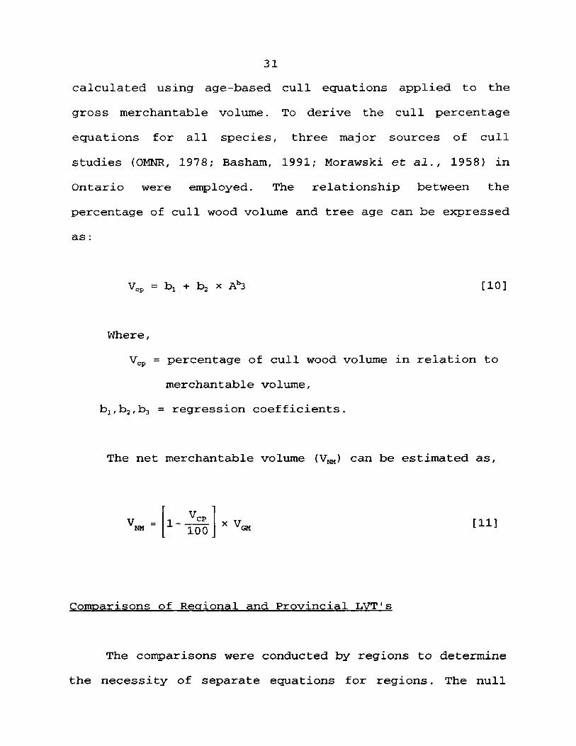
31

calculated using age-based cull equations applied to the

gross merchantable voliome. To derive the cull percentage

equations for all species, three major sources of cull

studies (OMNR, 1978; Basham, 1991; Morawski et al., 1958) in

Ontario were employed. The relationship between the

percentage of cull wood volume and tree age can be expressed

as :

= bi + t>2 X A^’3 [10]

Where,

V^p = percentage of cull wood volume in relation to

merchantable volume,

bi,b2,b3 = regression coefficients.

The net merchantable volume (V^M) can be estimated as.

V. NM 1-

V, CP 100

X V, GH [11]

Comparisons of Regional and Provincial LVT's

The comparisons were conducted by regions to determine

the necessity of separate equations for regions. The null

32

hypothesis was, for a given species, that the coefficients

(bi) in Equation [1] are not significantly different for

different regions and can be combined into one general

equation. The test criteria (t) is expressed as (Myers,

1990):

t = (bij - bik)/S.E.

Where:

bij = coefficient bi for region j,

bik = coefficient bi for region k,

S.E. = pooled standard error of coefficients bij and

bik.

The hypothesis is:

Ho: bij = bik, or I bij - biJ =0

Hi: bij / bik, or |bij - bikl ^0


Stem profile equations were fitted using the stem

analysis data available for this study and used in the

subsequent wood product mix modelling process. Several

33

published stem profile models (Demaerschalk, 1972; Max and

Burkhart, 1976; Kozak et al., 1969; Ormerod, 1973) were

examined and compared. These models are listed in Appendix C.

ACCURACY TESTING

For single-entry volume equations, accuracy testing was

conducted by coitparing the volumes estimated from the single-

entry volume ec[uations to the volumes from the standard

volume equations (Honer et al., 1983), as well as to the

stem analysis volumes. The stem analysis volumes used for the

testing were ass\imed to be the true values. The data sets for

which the single-entry volume accuracy was tested come from

the stem analysis data from Northwestern Ontario. Two species

were made available for the testing: i.e., jack pine and

black spruce.

All the tests were conducted by species and site class.

A similar procedure was applied to test and conpare the

height predication equations and age prediction equations.

The stem profile models were evaluated in order to

select the most appropriate one in the subsequent wood mix

modelling process. Diameter prediction, height prediction and

volume prediction by stem profile models were tested using

34

sample data and independent data sets. For the three

parameters (diameter, height and volume) tested, three

criteria (Cao et al., 1980) were employed.

In order to evaluate the overall performance of the stem

profile models tested, a method of ranking was employed. For

each individual tree species and each data set, a rank number

was assigned to each model according to the three criteria.

These ranks were then summarized for the three criteria for

each species and for each data set. The overall ranking for

each model was assigned based on the sxammed value for

criteria, and for both the sample data and the independent

data. The final overall ranking demonstrates the performance

of a model compared with the others.

THE DIMENSIONAL REQUIREMENTS OF WOOD PRODUCTS

The dimensional requirements for wood products vary due

to the impacts and constraints on forest industries. These

include changes in technology in wood processing and handling

systems, external economic influences on market demand, and

changes in Provincial or industrial policies which impact on

wood supply. Availability of raw material and accessibility

to the mill are also important in acceptance of the raw

35

material by each individual mill. Different mills utilize

different species or groups of species depending on the

products they produce. They set their own dimensional limits

based on the type of equipment in use and the ability of this

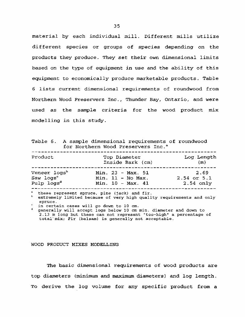
equipment to economically produce marketable products. Table

6 lists current dimensional requirements of roundwood from

Northern Wood Preservers Inc,, Thunder Bay, Ontario, and were

used as the sample criteria for the wood product mix

modelling in this study.

Table 6. A sample dimensional requirements of roundwood for Northern Wood Preservers Inc.®

Product Top Diameter Log Length Inside Bark (cm) (m)

Veneer logs'" Min. 23 - Max. 51 2.69 Saw logs'" Min. 11 - No Max. 2.54 or 5.1 Pulp logs*' Min. 10 - Max. 41 2.54 only

® these represent spruce, pine (jack) and fir. extremely limited because of very high quality requirements and only spruce. in certain cases will go down to 10 cm. generally will accept logs below 10 cm min. diameter and down to 2.13 m long but these can not represent "too-high" a percentage of total" mix; Fir (balsam) is generally not acceptable.


The basic dimensional requirements of wood products are

top diameters (minimtim and maximum diameters) and log length.

To derive the log volume for any specific product from a

36

tree, the lower and upper height limits along the bole are

required. These can be estimated from the known minimum and

maximum diameters using stem profile models.

Based on specific merchantability requirements for

various wood products, the procedure for modelling the wood

product mixes on a stand level is as following:

1. sort the stand information by species, dbh class and

site class when available,

2. decide the types of products being produced from the

stand and their corresponding dimensional requirements

and species preference,

3. determine the priority of products, i.e. the order of

various products to be generated from any given

species,

4. estimate the total height for each species and dbh

class from the dbh measurement using the corresponding

regional height-diameter equation,

5. starting from the product with the highest priority,

calculate the merchantable height limits for the

various products from the known minimum or maximiim top

diameters using a stem profile equation,

calculate the volumes for various products for each

species and dbh class; the basic steps at this stage

6.

37

can be described as: a) calculate the volume for the

first-order product for any given dbh class by

species, b) continue on the calculation of the

volumes for the second and third order products from

the remaining stem based on the merchantability limits

for these products, until the whole stem has been

broken into different products, and

7. sxjm the volumes of the stand:

V = Total volume of the stand,

n^ = Niomber of species in the stand,

TI2 = Number of dbh classes of the i*'*’ species,

nj = Number of wood product types to be modelled,

Vijk = Volume of the product type for the j*'*' dbh

class of the i'^’’ species.

The above procedure is illustrated in Figure 3. A

Fortran program (Appendix D) has been written to facilitate

the calculations for the above tasks.

[12]

Where:

38

Figure 3. Flowchart for wood product model.

39

This wood product mix model can also be equally applied

to individual trees. The basic elements in this system

include:

1. stem profile models to estimate the height limits (Hy

and HL) and the segment volume for any specific

product,

2. height prediction models used to estimate the total

heights from dbh classes,

3. merchantability limits for wood products.

40

RESULTS AND DISCUSSION

SINGLE-ENTRY VOLUME TABLE CONSTRUCTION

Model Selection

Height-diameter functions

The comparison of several height prediction models is

shown in Figure 4. The basal area function tends to flatten

out after dbh reaches a certain point. As dbh becomes larger,

the under-estimation of height by the basal area function

gets greater. The quadratic function fitted the data set well

within a certain range of dbh. It tends to drop down as dbh

gets larger. For very large diameter classes, the under-

estimation of height by the quadratic function is

significant. In contrast, both the exponential equation and

the Chapman-Richards function fitted the data sets very well,

and the shapes are biologically reasonable. Table 7 lists the

regression statistics (MSE and r^) for comparing the

exponential and Chapman-Richards models.

41

DBH (cm)

Figure 4. Comparison among several height prediction models for black spruce (site class X).

Table 7. Regression statistics for two height-dbh models

Species

Black spruce

Site Class n

Exponential

MSE (m)

Chapman-Richards

MSE (m) r^

Jack pine

X 1 2 3 4

X 1 2 3 4

1207 843 368 200

67

126 701 728 289 211

5.59053 4.40240 3.52584 2.35056 1.94378

7.69476 4.24996 2.82672 2.73158 2.76994

0.72248 0.62374 0.62822 0.52267 0.61505

0.71712 0.67735 0.59836 0.55114 0.85248

5.49918 4.36049 3.49706 2.33494 1.92646

7.24379 4.22817 2.82026 2.70972 2.70200

0.72724 0.62778 0.63227 0.52824 0.62435

0.73584 0.67946 0.59983 0.55628 0.85679

For the majority of data points in the dbh range of 10

to 40 cm, both the exponential and the Chapman-Richards

42

function yield almost the same predicted height (Figure 4),

The differences between these two models only lay outside the

10 to 40 cm dbh range.

In terms of bias and mean absolute differences (Table

8), the Chapman-Richards function performed slightly better.

However, it failed to produce good results for species with

small-sample data, such as black ash and red maple. This is

due to the fact that the Chapman-Richards function approaches

the asymptote too quickly when the dependent variable is only

weakly related to the independent variable (Huang et al. ,

1992) .

Table 8. Comparison between the exponential and the Chapman-Richards height prediction models

Species Site Class n Model e |e| SD (m) (m) (m)

Black spruce X

1

2

3

4

Jack pine X

1

2

3

4

1207 Exponential Chapman-Richards










.0202 1.8754 2.36

.0047 1.8523 2.34

.0109 1.6586 2.10

.0037 1.6433 2.09

.0029 1.4871 1.88

.0029 1.4795 1.86 -.0028 1.1882 1.53 -.0002 1.1779 1.52 -.0016 1.0304 1.38 .0029 1.0338 1.38 .0431 2.2544 2.76 .0059 2.1782 2.67 .0059 1.6355 2.06

-.0005 1.6343 2.05 .0020 1.2952 1.68

-.0002 1.2902 1.68 -.0020 1.3055 1.65 .0003 1.3095 1.64 .0424 1.2766 1.66

-.0049 1.2474 1.64

43

For most of the data sets, the model assumptions of

constant variance were approximately met by the exponential

function. Figure 5 shows the plot of studentized residuals

against the predicted height by the exponential function for

jack pine (site class X). It shows approximately homogenous

variance over the full range of predicted values.

Figure 5. The plot of studentized residuals against the predicted height for jack pine (site class = X).

44

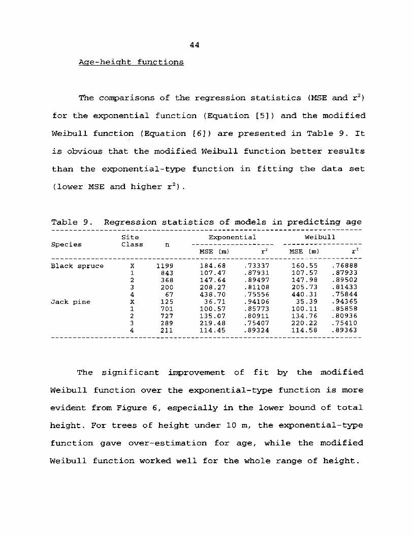
Age-height functions

The cort^arisons of the regression statistics (MSE and r^)

for the e3<ponential function (Equation [5] ) and the modified

Weibull function (Equation [6]) are presented in Table 9. It

is obvious that the modified Weibull function better results

than the exponential-type function in fitting the data set

(lower MSE and higher r^) .

Table 9. Regression statistics of models in predicting age

Exponential Weibull

MSE (m) MSE (m) r' Species

Black spruce

Jack pine

Site Class n

X 1 2 3 4 X 1 2 3 4

1199 843 368 200 67

125 701 727 289 211

184.68 107.47 147.64 208.27 438.70 36.71

100.57 135.07 219.48 114.45

.73337

.87931

.89497

.81108

.75556

.94106

.85773

.80911

.75407

.89324

160.55 107.57 147.98 205.73 440.31 35.39

100.11 134.76 220.22 114.58

.76888

.87933

. 89502

.81433

.75844

.94365

.85858

.80936

.75410

.89363

The significant improvement of fit by the modified

Weibull function over the exponential-type function is more

evident from Figure 6, especially in the lower bound of total

height. For trees of height under 10 m, the exponential-type

function gave over-estimation for age, while the modified

Weibull function worked well for the whole range of height.

45

TOTAL HEIGHT (m)

Figure 6. Plot of age prediction models for black spruce (site class X).

Accuracy of Sinale-Entrv Volume Equations

Table 10 shows the paired samples t-test between the

single-entry vol\ames and the stem analysis volumes. For all

site classes of jack pine and black spruce, except for black

spruce site class 3, the single-entry vol\jme equations fitted

the stem analysis data well with relative bias less than 10

percent. For jack pine, the differences between the single-

entry volumes and the stem analysis were insignificant for

site class X, 3, 4. As expected, the relative differences

46

between the single-entry and standard voliimes are small for

most cases (Table 11) , which demonstrated the consistency

between the single-entry and standard volume equations. These

cortparisons are also illustrated in Figures 7 and 8. Table 12

lists the comparisons of the standard volumes and the stem

analysis volumes.

Table 10. Comparisons between single-entry and stem analysis volumes

site Mean Relative Std. Species Class n Bias Volume Bias (%) Err. t

(m^) (m^) {mh

2-tail Sig.

Jack Pine

Black Spruce

X 1 2 3 4

X 1 2 3 4

120 238 172 156 84

175 312 210 83 37

0.0007 0.0062 -0.0098 -0.0042 -0.0024

0.0099 0.0021 -0.0019 -0.0024 -0.0023

0.0156 0.1802 0.1401 0.1290 0.0278

0.1666 0.0915 0.0567 0.0210 0.0236

4.49 3.44

-7.00 -3.26 -8.63

5.94 2.30

-3.35 -11.43 -9.75

0.001 0.003 0.003 0.002 0.002

0.

0. .002 001

0.001 0.000 0.000

0.95 2.12 -3.71 -1.92 -1.47

5.44 2.32 -3.02 -9.05 -5.68

0.345 0.035 0.000 0.056 0.146

0. 0,

0,

,000 ,021 003

0.000 0.000

Table 11. Comparisons between single-entry volumes and standard volumes

site Mean Relative Std. Species Class n Bias Volume Bias {%) Err.

(m^) (m^) (m^)

2-tail Sig.

Jack Pine X 120 -0.0001 0.0148 -0.68 1 238 -0.0037 0.1703 -2.17 2 172 -0.0113 0.1387 -8.15 3 156 -0.0079 0.1254 -6.30 4 84 -0.0004 0.0297 -1.35

Black Spruce X 175 0.0066 0.1633 4.04 1 312 0.0023 0.0917 2.51 2 210 0 0.0586 0 3 83 -0.0014 0.0220 -6.36 4 37 0 0.0259 0

0.000 0.002 0.003 0.001 0.001

0.001 0.001 0.000 0.000 0.000

-0.

-1.

-5. -5. -0,

6.

4. -0. -5. -0.

, 19 . 89 .45 ,88 .48

,77 ,07 , 04 ,37 06

0.846 0.067 0.000 0.000 0.630

0.000 0.000 0.969 0.000 0.952

Volume

(m''3)

47

Table 12. Comparisons between standard volumes and stem analysis volumes

Species Site Class n

Mean Bias Volijme

(m^)

Relative Bias (%)

Std. Err.

2-tail Sig.

Jack Pine

Black Spruce

X 1 2 3 4

X 1 2 3 4

120 238 172 156

84

175 312 210

83 37

0.0008 0.0099 0.0015 0.0036

-0.0020

0.0033 -0.0002 -0.0019 -0.0011 -0.0023

0.0156 0.1802 0.1401 0.1290 0.0278

0.1666 0.0915 0.0567 0.0210 0.0236

5.13 5.49 1.07 2.79

-7.19

1.98 -0.22 -3.35 -5.24 -9.75

0.000 0.001 0.001 0.001 0.001

0.001 0.001 0.000 0.000 0.000

1.

7 .

1. 2 .

-1.

78 28 41 64 66

2.36 0.42

-5.56 6.72

-5.93

0.078 0.000 0.162 0.009 0.101

0.019 0.675 0.000 0.000 0.000

Figure 7. Scatterplot of single-entry volumes versus stem analysis volumes for jack pine (site class 1).

Volume

(m''3)

48

Figure 8. Scatterplot of single-entry volximes versus standard volumes for jack pine (site class 1) ,

Two Approaches of Deriving Height Information

Zakrzewski (1993) proposed an approach of deriving

height using a central tree method. Maurer's (1993) approach,

on the other hand, is referred to as a site stratification

method.

For the site stratification method, the height-dbh

equations were derived by site class, hence, there is no

direct coitparison to the central tree method which generates

49

the equations by species. By employing the weighted average

criteria for all the site classes, however, it is easier to

compare these two approaches. From Table 13, it is apparent

that the site stratification method yielded better results

(lower MSE and higher r^) .

Table 13. Comparisons of the two height derivation approaches

site Stratification Method Central Species Criteria Tree

scX scl sc2 sc3 sc4 All Method

Jack pine n 126 701 728 289 211 1903 MSE 7.695 4.250 2.827 2.732 2.770 3.592 5.710 r^ 0.717 0.677 0.598 0.551 0.852 0.652 0.571

Aspen n 48 304 572 476 82 1386 MSE 6.561 6.092 4.113 4.165 4.712 4.648 9.405 r^ 0.865 0.758 0.783 0.743 0.599 0.757 0.620

Black spruce n 1207 843 368 200 67 2687 MSE 5.591 4.402 3.526 2.351 1.944 4.602 5.801 r^ 0.722 0.624 0.628 0.523 0.615 0.661 0.658

Comparative Analysis of Regional and Provincial LVT's

The two-tailed t-test statistics (Table 14) show that,

for jack pine, coefficients bi and ba in Equation [1] between

the two regions (Northwest and Northeast) were significantly

different except bj of site class 3. This result justified the

stratification of the single-entry volume equations for jack

pine by region. The height-diameter equations for black

spruce site classes 1, 2, 3 and 4 show overall insignificant

50

differences between the two regions. Only site class X tested

significantly different for both bi and 1>2 between the two

regions (Table 14).

Table 14. The statistics of 2-tail t-tests for testing the regression coefficients differences for the regional models

Species Site Class df

bx

Jack pine

Black spruce

X 1 2 3 4 X 1 2 3 4

382 874 495 176 109

1108 741 371 102 45

3.449** 6.999**

10.442** 3.401** 3.965** 6.111** 1.555 0.838 1.130 2.287*

4.329** 9.707** 7.056**

926 103** 178** 213* 044 030 360

significant at 95% confidence level Significant at 99% confidence level

The provincial single-entry volume equations were

constructed in the same way as the regional equations, by

combining the data sets from the regions across the province.

A further attempt was made to compare the provincial

equations to the regional equations to determine the

applicability of the models on a province-wide basis.

For black spruce, the provincial single-entry volume

equations gave very close vol\ime estimates as those by the

51

regional equations for both regions. The relative differences

between the provincial and the corresponding regional

estimates for all the site classes were less than 5 percent

(Table 15).

When the provincial volume equations for jack pine were

used to the Northeastern region, the differences were

apparent, especially between the provincial equations and the

Northeastern's equations (Table 15).

Table 15. Comparisons of regional and provincial LVT's

Species Site Region® n Class

Mean Vol. (m^)

Mean Diff (m^)

Relative Diff.(%)

Jack pine X

1

2

3

4

Black spruce X

1

2

3

4

NE NW NE NW NE NW NE NW NE NW NE NW NE NW NE NW NE NW NE NW

643 126

1048 701 267 727 68

289 12 56

1013 1207 643 843 378 368 109 200 27 67

.5245

.3923

.4622

.4356

.3869

.3343

.2809

.2681

.0998

.1456

.2525

.2415

.2002

.1714

.1418

.1380

.0859

.1051

.0641

.0613

.0005

.0013 -.0107 .0079

-.0235 .0023

-.0233 .0033

-.0123 -.0043 -.0046 .0025

-.0006 .0002

-.0009 .0017

-.0016 .0017

-.0031 .0009

0.10 0.33

-2.32 1.81

-6.07 0.69

-8.29 1.23

-12.32 -2.94 -1.82 1.04

-0.30 0.12

-0.63 1.23

-1.86 1.62

-4.84 1.47

^ NE = Northeastern Region; NW = Northwestern Region, ^ Defined as the volume predicted by the regional equation minus the

volume predicted by the provincial equation.

52


Comparisons Using The Sample Data

The summary statistics of the model performance for

diameter, height and volxome predictions for the sample data

are displayed in Table 16. To make it easier to compare these

models, all the criteria for the 12 species tested were

combined and recomputed using weighted average of the values

for each model. The biases were calculated by ignoring the

sign.

The bias in predicting diameters ranged from .1235 cm

for Demaerschalk' s model to .3278 cm for the model by Kozak

et al., while mean absolute difference in predicting

diameters ranged from .8617 cm for Max and Burkhart's model

to 1.0782 cm for the model by Kozak et al. In predicting

heights. Max and Burkhart's model did the best job for both

bias and the mean absolute difference (.0865 and .6852 m,

respectively), followed by Demaerschalk's model (.1174 and

.7390 m, respectively). With volume prediction,

Demaerschalk' s model performed the best for both bias and the

mean absolute difference (.0206 and .0485 m^, respectively),

followed by Ormerod's model (.0273 and .0533 m^'

respectively), then by Max and Burkhart's model (.0383 and

53

.0601 respectively). The model by Kozak et al. ranked the

lowest.

Table 16. Siimmary of bias, mean absolute difference, and standard deviation of several stem profile models for the sample data

Model Bias® MAD*^

Diameter Prediction (cm)

Demaerschalk (1972) .1235 Max and Burkhart (1976) .1973 Kozak et al. (1969) .3278 Ormerod (1973) .2449

.9786

.8617 1.0782 1.0675

1.4693 1.3380 1.5802 1.5328

Height Prediction (m)


.7390

.6852

.8070

.8269

Volxime Prediction (m^)

1.0475 1.0290 1.1271 1.1330


.0485

.0601

.0670

.0533

.0863

.1158

.1260

.0988

® The bias is defined as the measured values minus the predicted values. For volume prediction, stem analysis volumes (see MacLeod 1978, Appendix 1) were taken to be the true values.

^ Mean absolute differences of bias, standard deviation of bias.

Further comparisons were made among the models to

evaluate their ability to predict diameters, heights and

volumes in, relation to relative height along the tree bole.

The results are presented in Tables 17 and 18. Several trends

54

were revealed:

(1) It is apparent that the bias for both diameter and height

predictions for Max and Burkhart's model are significantly

smaller than those for the other models for both species at

most positions, especially at the lower portions of the bole.

This again indicates the superior predictive abilities of Max

and Burkhart's model in predicting top diameters and section

heights.

(2) In general. Max and Burkhart's model over-predicted

(negative bias) diameters and voliimes along the entire bole

but under-estimated (positive bias) heights for jack pine at

the middle positions. The other three models over-predicted

diameters, heights and volumes in the lower and upper bole,

but under-estimated in the middle positions

(3) There was no apparent differences among the four models

in predicting the section volumes.

55

Table 17. Summary of error of stem profile models by relative height class for jack pine

Section of Diameter (cm) Height (m) Volume (m^) relative n height Bias SD Bias SD Bias SD

0.0 s X < 0.1 525 0.1 < X < 0.2 272 0.2 < X < 0.3 267 0.3 < X < 0.4 272 0.4 s X < 0.5 264 0.5 < X < 0.6 268 0.6 < X < 0.7 267 0.7 < X < 0.8 264 0.8 < X < 0.9 265 0.9 < X < 1.0 521

All 3185

0.0 < X < 0.1 525 0.1 < X < 0.2 272 0.2 s X < 0.3 267 0.3 < X < 0.4 272 0.4 < X < 0.5 264 0.5 < X < 0.6 268 0.6 < X < 0.7 267 0.7 s X < 0.8 264 0.8 < X < 0.9 265 0.9 < X £ 1.0 521

All 3185

0.0 £ X < 0.1 525 0.1 £ X < 0.2 272 0.2 < X < 0.3 267 0.3 £ X < 0.4 272 0.4 < X < 0.5 264 0.5 £ X < 0.6 268 0.6 < X < 0.7 267 0.7 £ X < 0.8 264 0.8 £ X < 0.9 265 0.9 £ X £ 1.0 521

All 3185

0.0 < X < 0.1 525 0.1 £ X < 0.2 272 0.2 < X < 0.3 267 0.3 < X < 0.4 272 0.4 £ X < 0.5 264 0.5 £ X < 0.6 268 0.6 < X < 0.7 267 0.7£X<0.8 264 0.8£X<0.9 265 0.9 £ X £ 1.0 521

All 3185

Demaerschalk (1972)

.372 1.543 -.449 -.709 .778 -.973 -.663 1.075 -.797 -.408 1.642 -.373 -.042 1.106 .059 .221 .944 .356 .389 1.090 .525 .413 1.241 .532

-.164 1.363 .020 -.656 1.043 -.233 -.129 1.307 -.169 Max and Burkhart (1976)

-.082 1.001 -.152 -.170 .814 -.223 -.396 1.172 -.427 -.379 1.737 -.285 -.227 1.257 -.095 -.114 1.108 .055 -.039 1.231 .150 .006 1.349 .201

-.332 1.428 -.065 -.501 .968 -.151 -.234 1.206 -.103 Kozak et al. (1969)

.172 1.449 -.501 -.779 .966 -.949 -.672 1.256 -.718 -.377 1.744 -.271 -.007 1.218 .153 .239 1.037 .432 .349 1.163 .541 .280 1.305 .466

-.428 1.447 -.162 -.924 1.225 -.335 -.242 1.388 -.182

Ormerod (1973)

-.422 1.435 -.976 -1.286 1.000 -1.539 -1.084 1.281 -1.177 -.675 1.746 -.611 -.157 1.204 -.041 .255 1.005 .389 .565 1.124 .677 .718 1.255 .784 .245 1.352 .328

-.401 .923 -.119 -.258 1.379 -.284

.845 -.0025 .0087 1.000 -.0045 .0049 1.196 -.0053 .0096 1.441 -.0041 .0110 1.106 -.0022 .0099 .956 -.0003 .0077 .996 .0008 .0063

1.129 .0012 .0059 .870 .0004 .0050 .487 -.0009 .0033

1.088 -.0017 .0077

.484 -.0046 .0012 1.296 -.0009 .0044 1.588 -.0033 .0099 1.722 -.0039 .0124 1.347 -.0033 .0119 1.132 -.0022 .0101 1.062 -.0015 .0085 1.141 -.0009 .0075 .765 -.0009 .0060 .448 -.0007 .0031

1.102 -.0023 .0090

.861 -.0033 .0093 1.097 -.0063 .0086 1.316 -.0064 .0127 1.534 -.0048 .0132 1.202 -.0026 .0115 1.058 -.0006 .0090 1.085 .0004 .0073 1.214 .0006 .0066 .928 -.0005 .0057 .554 -.0018 .0038

1.157 -.0025 .0092

1.081 -.0048 .0095 .981 -.0100 .0108

1.171 -.0093 .0143 1.394 -.0068 .0141 1.059 -.0037 .0118 .925 -.0008 .0087 .968 .0011 .0067

1.107 .0021 .0059 .894 .0015 .0048 .468 -.0001 .0032

1.241 -.0030 .0102

56

Table 18. Summary of error of stem profile models by relative height class for black spruce

Section of Diameter (cm) Height (m) Volume (m^) relative n height Bias SD Bias SD Bias SD

0.0 < X < 0.1 142 0.1 s X < 0.2 89 0.2 < X < 0.3 90 0.3sx<0.4 95 0.4<x<0.5 94 0.5 s X < 0.6 89 0.6 £ X < 0.7 87 0.7£X<0.8 88 0.8<x<0.9 88 0.9 s X £ 1.0 169

All 1031

0.0 < X < 0.1 142 0.1 < X < 0.2 89 0.2 £ X < 0.3 90 0.3£X<0.4 95 0.4<x<0.5 94 0.5£X<0.6 89 0.6 £ X < 0.7 87 0.7£X<0.8 88 0.8 £ X < 0.9 88 0.9 £ X £ 1.0 169

All 1031

0.0 £ X < 0.1 142

0.1 < X < 0.2 89 0.2£X<0.3 90 0.3 £ X < 0.4 95 0.4<x<0.5 94 0.5<x<0.6 89 0.6 £ X < 0.7 87 0.7£X<0.8 88 0.8£X<0.9 88 0.9 £ x £ 1.0 169

All 1031

0.0 £ X < 0.1 142 0.1 £ X < 0.2 89 0.2£X<0.3 90 0.3 £ X < 0.4 95 0.4£X<0.5 94 0.5 < X < 0.6 89 0.6£X<0.7 87 0.7£X<0.8 88 0.8<x<0.9 88 0.9 £ x £ 1.0 169

All 1031

Demaerschalk (1972)

.210 1.505 -.550 -.769 .512 -.951 -.387 .505 -.448 -.007 .475 .015 .138 .562 .192 .307 .629 .387 .348 .660 .415 .241 .727 .295 .074 .654 .121

-.106 .464 -.013 .006 .829 -.076

Max and Burlchart (1976)

-.053 .830 -.169 -.097 .496 -.175 -.096 .525 -.107 -.023 .506 .018 -.125 .590 -.108 -.134 .645 -.075 -.136 .688 -.051 -.064 .731 .006 -.024 .643 .025 -.175 .475 -.036 -.097 .623 -.070 Kozalc et al. (1969)

.053 1.507 -.615

-.783 .625 -.937 -.353 .573 -.405 .049 .493 .075 .177 .556 .232 .287 .604 .371 .236 .644 .317 .009 .719 .082

-.330 .680 -.223 -.461 .570 -.196 -.129 .855 -.158

Ormerod (1973)

.235 1.522 -.543 -.756 .463 -.943 -.385 .474 -.452 -.025 .474 -.005 .126 .573 .177 .297 .647 .380 .345 .666 .412 .236 .725 .292 .074 .651 .121

-.107 .461 -.013 .006 .830 -.079

.908 -.0008 .0026

.575 -.0029 .0031

.582 -.0021 .0024

.543 -.0007 .0016

.717 .0002 .0015

.669 .0006 .0016

.662 .0008 .0006

.658 .0006 .0015

.505 .0003 .0012

.266 .0001 .0006 .740 -.0004 .0022

.455 -.0013 .0033

.875 0 .0019

.899 -.0007 .0018

.765 -.0005 .0016

.750 .0004 .0016

.684 -.0005 .0018

.600 -.0005 .0018

.530 -.0013 .0016

.443 0 .0012

.267 0 .0006

.628 -.0004 .0019

.998 -.0012 .0024

.705 -.0033 .0038

.665 -.0023 .0027

.571 -.0007 .0018

.630 .0001 .0015

.671 .0004 .0016

.680 .0005 .0015

.678 .0002 .0014

.512 -.0002 .0013

.312 -.0003 .0007 .768 -.0007 .0023

.883 -.0007 .0027

.536 -.0028 .0029

.560 -.0020 .0022

.543 -.0006 .0015

.627 .0002 .0015

.680 .0006 .0016

.665 .0008 .0016

.660 .0006 .0014

.505 .0003 .0012

.266 .0001 .0006 .731 -.0003 .0021

57

Comparisons Using The Independent Data

The preceding results described the fit of the four stem

profile models to the data used to build the models. For the

stem profile models tested, independent stem analysis data

sets were also used to validate the model performance to

determine their applicability beyond the sample data. Two

sources of independent data sets were used: (1) the reserved

FMI data, and (2) the stem analysis data from Central

Ontario.

As in the tests for the sample data. Max and Burkhart's

model achieved better results than the other models in

predicting diameters and heights. Moreover, Max and

Burkhart's model was the best for volume prediction for the

independent data. These results are shown in Table 19.

58

Table 19. Summary of bias, mean absolute difference, and standard deviation of several stem profile models for the independent data

Model Bias MAD SD

Diameter Prediction (cm)


1.5007 1.3584 1.6117 1.6372

2.0366 1.9075 2.1507 2.1716

Height Prediction (m)


1.0990 1.0187 1.1791 1.2160

1.4528 1.4322 1.5468 1.5835

Volume Prediction* (m^)


.0092

.0090

.0098

.0104

.0162

.0170

.0179

.0172

stem analysis data in Northwestern Ontario.

The ranking results (Table 20) show that Max and

Burkhart's model ranked the highest in ability to predict top

diameters and heights. Demaerschalk's model ranked second,

followed by Ormerod's model and the model by Kozak et al.

With volume prediction, however, Demaerschalk's model ranked

the highest, followed closely by Max and Burkhart's model,

then by Kozak et al.'s model. Ormerod's model gave the

poorest results for volume prediction.

59

Table 20. Overall rankings of the four models for diameter, height and volume prediction

Model Test data Bias

Ranking*

MAD SD Sum

Overall ranking

Diameter

Demaerschalk (1972)

Max and Burkhart (1976)

Kozak et al. (1969)

Ormerod (1973)

sample 22 27 26 75 independent 26 27 25 78 All 48 54 51 155 sample 27 12 13 52 independent 21 11 10 42 All 48 23 23 94 sample 39 42 44 125 independent 26 33 37 96 All 65 75 81 221 sample 32 39 37 108 independent 27 31 28 86 All 59 70 65 194

Demaerschalk (1972)

Max and Burkhart (1976)

Kozak et al. (1969)

Ormerod (1973)

sample independent All sample independent All sample independent All sample independent All

Height

26 26 52 17 25 42 40 19 59 37 30 67

29 24 51 12 20 32 41 28 69 38 28 66

27 23 50 16 18 36 41 34 75 36 25 61

82 73

155 45 63

108 122 81

203 111 83

194

volume

Demaerschalk (1972)

Max and (1976)

Kozak et (1969)

Burkhart

al.

Ormerod (1973)

sample 22 21 19 62 independent 17 16 16 49 All 39 37 35 111 sample 31 28 31 90 independent 10 10 9 29 All 41 38 40 119 sample 36 37 39 112 independent 7 7 7 22 All 43 44 45 134 sample 31 34 31 96 independent 18 17 17 52 All 49 51 49 148

All species combined.

60

A test to compare Demaerschalk' s model and Max and

Burkhart's model to the standard volume equations (Honer et

al., 1983) was conducted. The results are shown in Table 21.

It is apparent that, for most species, both models gave

satisfactory results. For black spruce, balsam fir, white

birch and white cedar, however, the biases are relative

large. Another trend shown in Table 21 is that the over-

estimation becomes greater as the dbh class gets larger.

Generally, Demaerschalk's model performed better in voliome

prediction for.softwood species, while the model by Max and

Burkhart demonstrated superior results for hardwood species.

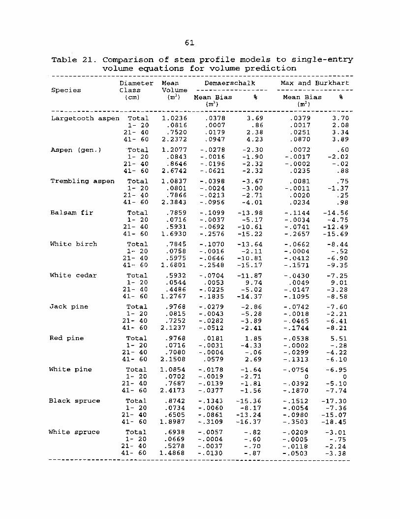
61

Table 21. Comparison of stem profile models to single-entry volume equations for volume prediction

Species Diameter Class (cm)

Mean Volume

(m^)

Demaerschalk

Mean Bias (m^)

Max and Burkhart

Mean Bias (m-

Largetooth aspen Total 1- 20

21- 40 41- 60

Aspen (gen.)

Trembling aspen

Balsam fir

White birch

White cedar

Jack pine

Red pine

White pine

Black spruce

White spruce

Total 1- 20

21- 40 41- 60

Total 1- 20

21- 40 41- 60

Total 1- 20

21- 40 41- 60

Total 1- 20

21- 40 41- 60

Total 1- 20

21- 40 41- 60

Total 1- 20

21- 40 41- 60

Total 1- 20

21- 40 41- 60

Total 1- 20

21- 40 41- 60

Total 1- 20

21- 40 41- 60

Total 1- 20

21- 40 41- 60

1.0236 .0816 .7520

2.2372

1.2077 .0843 .8646

2.6742

1.0837 .0801 .7866

2.3843

.7859

.0716

.5931 1.6930

.7845

.0758

.5975 1.6801

. 5932

.0544

.4486 1.2767

.9768

.0815

.7252 2.1237

.9768

.0716

.7080 2.1508

1.0854 .0702 .7687

2.4173

. 8742

.0734

.6505 1.8987

.6938

.0669

.5278 1.4868

. 0378

.0007

.0179

.0947

.0278

.0016

.0196

.0621

. 0398

.0024

.0213

.0956

.1099

.0037

.0692

.2576

. 1070

. 0016

.0646

.2548

. 0704

.0053

. 0225

. 1835

.0279

.0043

.0282

.0512

.0181

.0031

.0004

.0579

. 0178

. 0019

. 0139

.0377

. 1343

.0060

.0861

.3109

, 0057 0004 0037 0130

3.69 .86

2.38 4.23

-2.30 -1.90 -2.32 -2.32

-3.67 -3.00 -2.71 -4.01

-13.98 -5.17

-10.61 -15.22

-13.64 -2.11

-10.81 -15.17

-11.87 9.74

-5.02 -14.37

-2.86 -5.28 -3.89 -2.41

1.85 -4.33 -.06 2.69

-1.64 -2.71 -1.81 -1.56

-15.36 -8.17

-13.24 -16.37

-.82 -.60 -.70 -.87

. 0379

. 0017

.0251

.0870

.0072

.0017

.0002

.0235

.0081

.0011

. 0020

.0234

.1144

.0034

.0741

.2657

. 0662

. 0004

.0412

.1571

. 0430

.0049

.0147 . 1095

.0742

.0018

.0465

.1744

.0538

.0002

.0299

.1313

.0754 0

.0392

.1870

.1512

.0054

.0980

.3503

.0209

.0005

.0118

.0503

3.70 2.08 3.34 3.89

. 60 -2.02 -.02

.88

.75 -1.37

.25

.98

-14.56 -4.75

-12.49 -15.69

-8.44 -.52

-6.90 -9.35

-7.25 9.01

-3.28 -8.58

-7.60 -2.21 -6.41 -8.21

5.51 -.28

-4.22 -6.10

-6.95 0

-5.10 -7.74

-17.30 -7.36

-15.07 -18.45

-3.01 -.75

-2.24 -3.38

62


The wood product mix model was developed to estimate

volumes for various wood products generated from individual

stands or trees. Obviously, the wood product mix model does

not depend on any specific criteria. The following example

demonstrates the application of the model. The stand

information (Table 22) was taken from stand "Kelvin 2656"

(Maurer, 1994).

Table 22. Diameter distributions of input stand

Dbh Class (cm)

Stems Per Hectare

Trembling aspen

Balsam fir

White birch

Jack pine

Black spruce

White spruce

6 8

10 12 14 16 18 20 22 24 26 28 30 32 34 36 38 40 42 44 46 56

12 9

18 25 21 29 27 10 13 15 7 1 4 3 4 2 1

141 96 51 35 42 24 13 5 8 4

32 41 14 21 16 3 8

13 8 8 9 9

16 9 3 1 3 4

16 10 35 26 4 9 3 2

3 1

16

8 3 3 6 7 3 1 1 2

63

The results of wood product mixes modelled are presented

in Table 23. These volumes were generated from Demaerschalk'

(1972) stem profile model. Table 24 lists the comparisons

between the volvimes and those obtained from the standard

volume equations (Honer et al. , 1983). It is apparent, in

terms of voliime estimation, that the wood product mix model

was consistent to the voliame equation approach.

Table 23. Output of stand modelling*

Ave. Ave. Ave. Volumes For Products {ra’) Spp. Dbh Height Volume n

(cm) (m) (m^) Veneer Sawlog# Pulp# Chips

AT 26.89 21.84 BF 9.89 8.27 BW 12.01 12.36 PJ 25.83 19.73 SB 13.45 11.89 SW 18.12 12.81

ALL 15.73 13.14

.6266 201 .00

.0501 420 .00

.0764 137 .00

.5158 84 .00

.1049 110 1.22

.2242 52 3.57

.2231 1004 4.79

.00 .00 125.95 10.10 .00 10.95

.00 .00 10.46

.00 41.04 2.29

.00 7.07 3.25

.00 7.06 1.03 10.10 55.17 153.93

* This table only shows the summary information for the species and the stand. The merchantability limits are taken from Table 6.

# Because of the similar dimensional requirements, these two products can be assigned either way depending on the preference of the products.

Table 24. Volume comparisons between wood product mix model and standard volume equations

Species Volume Estimates (m^)

Product model Honer et al. Bias %

Trembling aspen Balsam fir White birch Jack pine Black spruce White spruce All

125.95 21.05 10.46 43.33 11.54 11.66

223.99

122.63 20.33 10.52 41.70 10.66 11.53

217.37

3.32 0.72

-0.06 1.66 0.84 0.13 6.62

2.64 3.42

-0.57 3.83 7.28 1.11 2.96

64

CONCLUSIONS AND RECOMMENDATIONS

CONCLUSIONS

In deriving the height variable for the construction of

single-entry volume tables, the site stratification method

demonstrated superior performance over the central tree

method. The use of a site stratified height-dbh equation

greatly reduced the variation of height prediction within a

region, thus leading to a wider application for the

geographic area in which the equation was derived. For black

spruce in the two northern Ontario regions, the provincial

single-entry volume tables will apply nearly equally well as

the regional tables. Generally, there is a wider variation in

the height-dbh relationship between the two regions for jack

pine and the other species tested (Appendix A) . For these

species, the applications of the single-entry volume

equations on a province-wide basis cannot be justified.

The exponential height function of Height = 1.3 + bi x

exp(b2/Dbh), as proved by many others (Maurer, 1993; Arabatzis

and Burkhart, 1992), produced satisfactory height estimates

for most tree species tested in this study. Another height-

65

diameter function deserving some attention is the Chapman-

Richards function suggested by Huang et al. (1992). This

function can be very useful when fitted to large sample data

sets. Unfortunately, it failed to fit the height-diameter

relationship well for some species with small sample data

sets.

In predicting age, the modified Weibull function of Age

= bi X exp(b2 X Heights’S) showed a significant in^rovement over

the exponential-type function of Age = 1.3 + b^ x exp(b2 x

Height). It produced reasonable age estimates for the whole

range of height class observed in this study.

The wood product mix model, based on the stem profile

equations and dbh distributions, offers an efficient way of

estimating merchantable volumes by wood products from

merchantable stands. It is useful in evaluating alternative

uses of timber resources. The wood product mix model can be

applied to any merchantable stands in accordance with varying

product demands and dimensional requirements. The model

itself is flexible, and capable of estimating various wood

products, regardless of the specific criteria for a given

product. With the Fortran program written to facilitate the

calculations, the model is easy and straightforward to apply.

66

Of the stem profile models tested, the segmented

polynomial model by Max and Burkhart (1976) proved to be the

most accurate and precise in predicting top diameters and

section heights, especially at the lower portions of the tree

bole, while the model derived from the logarithmic volume

equation by Demaerschalk (1972) ranked the highest overall

for volume prediction, followed closely by Max and Burkhart's

model. In general, Demaerschalk's model gave better volume

prediction for softwood species, while the model by Max and

Burkhart was superior for hardwood species.

Generally, all the stem profile equations over-estimated

diameters and volumes to some extent due to the

re transformation of squared diameter to diameter (Czaplewski

and Bruce, 1990) . This over-estimation becomes more apparent

when the diameters of trees get larger. This is especially

true for some species such as black spruce and balsam fir.

However, for the range normally observed in Ontario for these

species, this over-estimation was usually less than 10

percent.

RECOMMENDATIONS FOR FUTURE WORK

Due to the limitations of the data sets available, the

single-entry volume table initiative was limited to the two

67

northern regions of Ontario. To complete the above task for

the whole province, further work is needed to collect data

from the other two regions (Central and Southern), and

continue the modelling process using the methodology

demonstrated in this thesis. For some species with

insufficient sample data and for other species without any

data, additional or new data is required to adequately fit

the height prediction models and the age prediction models.

For some tree species, the variation of height within a

region might be too large. It would be desirable to produce

sub-regional single-entry voliame tables (such as forest site

regions defined by Hills (1958)) when the variation of

height-diameter relationships within a region proves

significant, provided that the appropriate data sets for the

subregions are available.

All the stem profile models were fitted by using data

from the FMI data bank, new stem analysis data is also

required to make these equations more adequate and more

reliable. For species such as black spruce, balsam fir, white

birch and white cedar, additional stem analysis data is

needed. It is recommended that the stem profile models by

regions and species be fitted when the data sets are made

available.

68

In this project, the wood product mix model was

basically for the estimation of various wood products for

both a single tree and a stand. Further work to develop a

system to model primary breakdown of trees or stands for

optimal solutions based on the concept of global

optimization, in which overall mill flow, product mixes and

other global criteria will be considered is recommended.

Actual data for merchantable stands was unavailable. The

lack of real data sets was a handicap to model dbh

distributions found in merchantable stands. These dbh

distributions, when available, can be used by combining the

wood product mix model to describe the various combinations

of raw products to be generated from merchantable stands.

69

LITERATURE CITED

Alemdag, I. S. 1990. Merchantable voliome conversion factors and taper equations for commercial tree species of Ontario. PNFI, Chalk River, Ont. Tech. Rept. 8 pp.

Alemdag, I. S. 1988. A ratio method for calculating stem volume to variable merchantable limits, and associated taper equations. For. Chron. 64:18-26.

Alemdag, I. S. and T, G. Honer. 1977. Metric relationships between breast-height and stiamp diameters for eleven tree species from eastern and central Canada. Can. For. Serv., For. Manage. Inst., Ottawa, Ont. Info. Rept. FMR- X-49M.

Arabatzis, A. A. and H. E. Burkhart. 1992. An evaluation of saitpling methods and model forms for estimating height- diameter relationship in loblolly pine plantations. For. Sci. 38(1):192-198.

Avery, T. E. and H. E. Burkhart. 1983. Forest measurements. McGraw Hill Book Company. New York. 331 pp.

Basham, J. T. 1991. Stem decay in living trees in Ontario's forests. Great Lakes For. Cent., For. Can., Sault Ste Marie. Info. Rept. O-X-408. 64 pp.

Biging, D. S. 1988. Estimating the accuracy of volume equations using taper equations of stem profile. Can. J. For. Res. 18:1002-1007.

Bonner, G. M. 1974. Estimation versus measurement of tree heights in forest inventories. For. Chron. 200 pp.

Broad, L. R. and G. C. Wake. 1995. Derivative based methods for constructing volume-ratio and taper equations. For. Sci. 41(1): 157-167.

Burkhart, H. E. 1977. Cubic foot volume of loblolly pine to any merchantable top diameter. South. J. Appl. For. 1:7- 9.

Byrne, J. C. and D. D. Reed. 1986. Complex compatible taper and volume estimation systems for Red and Loblolly pine. For. Sci. 32:423-443.

70

Cao, Q. V., H. E. Burkhart and T. A. Max. 1980. Evaluation of two methods for cubic-volume prediction of loblolly pine to any merchantable limit. For. Sci. 26:71-80.

Chapman, H. H, and W. H. Meyer. 1949. Forest Mensuration. McGraw-Hill Book Company. New York. 522 pp.

Clutter, J. L. 1980. Development of taper functions from variable-top merchantable volume equations. For. Sci. 26:117-120.

Czaplewski, R. L. and D. Bruce. 1990. Retransformation bias in a stem profile model. Can. J. For. Res. 20:1623-1630.

Czaplewski, R. L., A. S. Brown and D. G. Guenther. 1989a. Estimating merchantable tree volume in Oregon and Washington using stem profile models. U.S. Rocky Mt. For. Range Exp. Stn., Fort Collins, Co. Res. Pap. RM- 286. 15 pp.

Czaplewski, R. L., A. S. Brown and R. C. Walker. 1989b. Profile models for estimating log end diameters in the Rocky Mountain region. U.S. Rocky Mt. For. Range Exp. Stn., Fort Collins, Co. Res. Res. Pap. RM-284. 7 pp.

Demaerschalk, J. P. and A. Kozak. 1977. The whole-bole system; a conditional dual equation system for precise prediction of tree profiles. Can. J. For. Res. 7:488- 497 .

Demaerschalk, J. P. 1973. Integrated systems for the estimation of tree taper and volume. Can.. J. For. Res. 3(1);90-94.

Demaerschalk, J. P. 1972. Converting volume equations to compatible taper equations. For. Sci. 18(3):241-245.

Flewelling, J. W. 1993. Variable-shape stem-profile predictions for western hemlock. Part II. Predictions from DBH, total height, and upper stem measurements. Can. J. For. Res. 23:537-544.

Freese, F. 1960. Testing Accuracy. For. Sci. 6:139-145.

Gillis, M. D. and J. A. Edwards. 1988. Volume compilation procedures in forest management inventories. PNFI. For. Can., Info. Rept. PI-X-79. 20 pp.

Gribko, L. S. and H. V. Wiant, Jr. 1992. A SAS* template

71

program for the accuracy test. Compiler 10(1):48-51.

Gregoire, T. G, H. T. Valentine and G. M. Furnival. 1986. Estimation of bole volume by importance sampling. Can. J. For. Res. 16:554-557.

Grosenbaugh, L. R. 1966. Tree form: definition, interpolation, extrapolation. For. Chron. 42(4)444-457.

Hills, G. A. 1958. Soil-forest relationships in the site regions of Ontario. First North America Forest Soils Conference Proc., East Lansing 1958. Bull. Agr. Expt. Sta., Mich. State Univ. pp. 190-212.

Honer, T. G., M. F. Ker and I. S. Alemdag. 1983. Metric timber tables for the commercial tree species of Central and Eastern Canada. Can. For. Serv., Marit. For. Res. Cent., Fredericton, NB. Info. Rept. M-X-140, 139 pp.

Honer, T. G. 1967. Standard volume tables and merchantable conversion factors for the commercial tree species of Central and Eastern Canada. For. Manag. Res. and Serv, Inst. Ottawa; Info. Rep. FMR-X-5, 21 pp + appendices.

Honer, T. G. 1964. The use of height and squared diameter ratios for the estimation of merchantable cubic-foot volume. For. Chron, 40:423-331.

Huang, S., S. J. Titus and D. D. Wiens. 1992. Comparison of nonlinear height-diameter functions for major Alberta tree species. Can. J. For. Res. 22:1297-1304.

Husch, B., C. I, Miller and T. W. Beers. 1982. Forest mensuration. 3rd Ed. John Wiley and Sons Inc. New York. 373 pp.

Kavanagh, J, 1983. Stem analysis: sampling techniques and data processing. Sch. of For., Lakehead Univ., M.Sc thesisThunder Bay, Ont,, 88 pp + appendices,

Kozak, A. 1988. A variable-exponent taper equation. Can. J. For. Res. 18: 1363-1368.

Kozak, A., D. D. Munro and J. H. G. Smith. 1969. Taper functions and their application in forest inventory. For. Chron. 45(4):278-283.

MacLeod, D. A. 1978. The Forest Management Institute tree data bank. Dept, of Envir., Can. For. Serv. FMR-X-112.

72

15 pp.

Martin, A. J. 1984. Testing volume equation accuracy with water displacement techniques. For. Sci. 30{l):41-50.

Martin, A. J. 1981. Taper and volume equations for selected Appalachian hardwood species. USDA, For. Serv. Northeast. For. Exp. Stn., Broomall, PA. Res. Pap. NE- 490. 22 pp.

Maurer, N. L. 1994. Stand volume inventory information for Northeastern Ontario. OMNR, Timmins, Ont. NEST Tech. Rept. TR014. 1135 pp.

Maurer, N. L. 1993. Deriving local tree volume information. OMNR, Timmins, Ont. NEST Tech. Rept. TR-010. 41 pp.

Max, T. A. and H. E. Burkhart. 1976. Segmented polynomial regression applied to taper equations. For. Sci. 22:283- 289.

McDonald, P. M. 1982. Local voliame tables for pacific madrone, tanoak, and California black oak in north- central California. Pac. Southwest For. Range Exp. Stn. USDA For. Serv., Berkeley, Califoria. Note, No. PSW-362, 6 pp.

McTague, J. P. and R. L. Bailey. 1987. Simultaneous total and merchantable volume equations and a compatible taper fxinctions for loblolly pine. Can. J. For. Res. 17:87-92.

Morawski, Z. J. R., J. T. Basham and K. B. Tuner. 1958. Cull studies. A survey of a pathological condition in the forests of Ontario. Div. of Timber, Ont. Dept, of Lands and For. Toronto, Rept. No. 25. 96 pp.

Munro, D. D. and J. P. Demaerschalk. 1974. Taper-based verses vol\ime-based compatible estimating systems. For. Chron. 50(5):197-199.

Murchison. H. G. 1984. Efficiency of multi-phase and multi- stage sampling for tree heights in forest inventory. Univ. of Minnesota, Fac. of Grad. Sch., St. Paul. MN. Ph.D. Thesis. 158 pp.

Myers, R. H. 1990. Classic and Modern regression with applications. 2nd Ed. PWS-Kent Publ. Co. Boston. 488 pp.

OMNR. 1992. Forest growth and yield: a master plan for

73

Ontario. OFRI, OMNR, Sault Ste Marie, Ont. Draft. 109 pp. (Cited in Maurer, 1993).

OMNR. 1978. Cull survey tables (metric). OMNR. 51 pp.

Ormerod, D. W. 1973. A siirple bole model. For. Chron. 49:136- 138.

Plonski, W. L. 1981. Normal yield tables (metric) for major forest species of Ontario. OMNR. 40 pp.

Rauscher. H. M. 1986. Testing prediction accuracy. USDA For. Serv. Gen. Tech. Rep. NC-107. 19 pp.

Reynolds, M. R. Jr. 1984. Estimating the error in model predictions. For. Sci. 30(2):454-469.

Sterba, H. 1980. Stem curves - a review of the literature. For. Abstr. 41:141-145.

Weisberg, S. 1980. Applied linear regression. Wiley Press, New York. 283 pp.

Wiant, H. V. Jr. 1993. DOSATEST for testing accuracy. Compiler ll(3):28-29.

Wiant, H. V. Jr., G. B. Wood and J. A. M. Miles. 1989. Estimating the voliime of a radiata pine stand using importance sampling. '

Wood, G. B. and H. V. Wiant Jr. 1990. Estimating the volume of Australian hardwoods using centroid sampling. Aust. For. 53:271-274.

Yang, R. C., A. Kozak and J. H. G. Smith. 1978. The potential of Weibull-type functions as flexible growth curves. Can. J. For. Res. 8:424-431.

Zakrzewski, V. 1993. Deriving localized tree volume information. OFRI. Sault Ste Marie, Ont. 3 pp.

APPENDICES

75

APPENDIX A LIST OF THE SPECIES STUDIED

Common name Latin name

Softwoods

Species code

White cedar Balsam fir Jack pine Red pine White pine Black spruce White spruce Tamarack

Black ash Largetooth aspen Aspen (gen.) Trembling aspen Beech White birch Yellow birch Red maple Sugar maple Balsam poplar

Thuja occidentalis L. CE Abies balsamea (L.) Mill. BF Pinus banksiana Lamb. PJ Pinus resinosa Ait. PR Pinus strobus L. PW Picea mariana (Mill.)B.S.P. SB Picea g-lauca (Moench) Voss SW Larix laricina (Du Roi) K. Koch LA

Hardwoods

Fraxinus nigra Marsh. AB Populus grandidentata Michx. AL Populus AS Populus tremuloides Michx. AT Fagus grandifolia Ehrh. BE Betula papyrifera Marsh. BW Betula alleghaniensis Britton. BY Acer rubrum L. MR Acer saccharum Marsh. MS Populus balsamifera L. PB

76

APPENDIX B SITE CLASS ASSIGNMENT EQUATIONS FOR MAJOR TREE

SPECIES IN ONTARIO*

No Equations Suitable Species

scX=exp(4

scl=exp(3 sc2=exp(3

sc3=exp(4 sc4=exp(4

scX=exp(3

scl=exp(3 sc2=exp(3

sc3=exp(3

sc4=exp(3

scX=exp(3

scl=exp(3, sc2=exp(3 . sc3=e3<p (3 . sc4=e3qp (2 ,

scX=exp(3, scl=exp(3.

sc2=exp(3. sc3=exp(3, sc4=exp(2.

scX=exp(3.

scl=exp(3. sc2=exp(3. sc3=exp(3.

sc4=exp(3.

050409-48.36061*AGE-^ °)

8513-50.0826*AGE'^ °)

501411-52.2586*AGE"" °)

2542-16.0182*AGE’°-^) 2371-20.42529*AGE"°'^)

-1.0 . 823071-22.44245*AGE . 6544-24.463*AGE-^-°)

.7298-14.223 *AGE'°-''^)

. 6209-16.13 6*AGE’° ’'^)

. 4644546-20.58747*AGE'° '^^

. 647108-27.9734*AGE‘^ °)

.470401-24.463*AGE-^°)

. 392001-31.516*AGE'^ °)

. 169538-32.53107*AGE‘^ °}

. 913733-38.07934*AGE-^°)

. 747122-11.98245*AGE‘°-’^)

. 4052-25.105*AGE‘^ °)

.269-27.413*AGE-^ °)

. 1146-30.748*AGE’^ ®)

.881159-38.87831*AGE-^ °)

, 575054-16.94687*AGE‘°-^^)

.4659-20.05*AGE'°-’^) ,3579-23.78*AGE-° ''^) 4109-32.713*AGE’°-'^^)

183022-37.27952*AGE"°-'^^)

)

Red pine.

White pine

Balsam poplar.

Aspen (gen.)

Black ash, Red oak

Black cherry. Elm,

White birch. Yellow birch. Red maple.

Sugar maple

Jack pine, Scots pine. Trembling aspen.

White spruce

Balsam fir.

White cedar. Black spruce

From Maurer (1993)

77

APPENDIX C LIST OF STEM PROFILE MODELS

The four stem profile models tested in this study are listed bellow. According to Martin (1981), each model is presented by: (a) basic stem profile equation, (b) height prediction equation, and (c) voltime prediction equation.

To simplify the text, the use of the following notations will be consistent in this appendix. Variables not listed are defined where they are used.

d: top diameter inside bark at height h,

D: diameter outside bark at breast height (1.3 m) ,

h: height above the ground to top diameter d,

H: total tree height from ground to tip,

HLI lower limit of tree height for voliime calculation,

Hy: upper limit of tree height for volume calculation,

VL: log volume of tree excluding bark between any two

height limits,

bi,Ci! regression coefficients peculiar to specific

equations.

1. Demaerschalk's (1972) model

[Cl.a]

h = H - d

■

b. [Cl.b]

(10*"') (D^"^) (H^^)

78

(0.0000785) (10^^‘) -X/) _ [Cl.c]

Where:

Z = 2 ba + 1

Xi = H - HL

X2 = H - Hu

2. Max and Burkhart's (1976) model

[C2.a]

Where:

ai = join points; the upper point is i=l,

the lower point is i=2

11 = 1, if h/H < ai

= 0, otherwise

12 = 1, if h/H < 32

0, otherwise

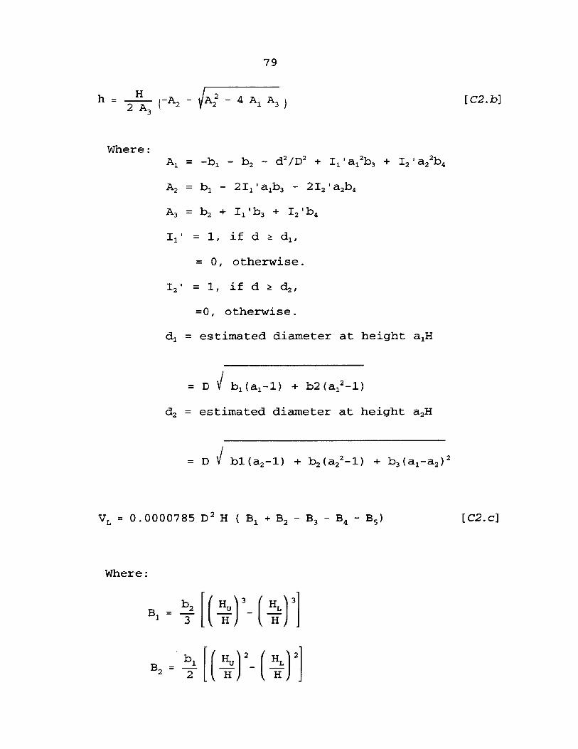
79

h = ^ |-A, - /A| - 4 AJ A, ) tC2.b]

Where: Ai = -bi - ba - d^/D^ + li'ai^ba + Iz'a-z^hi

A2 = bj^ — 2 Ij^ ’ Sib3 — 212' a2b^

A3 = b2 + Ii' b3 + I2' b^

Ii' =1, if d ^ di,

= 0, otherwise.

I2' =1, if d > dj,

=0, otherwise.

di = estimated diameter at height a^H

= D V bi(ai-l) + b2(ai^-l)

d2 = estimated diameter at height ajH

= D V bl{a2-l) + b2(a2'“-l) + b3(ai-a2)^

VL = 0.0000785 H ( + 83 - B3 - - B5) [C2.c]

Where:

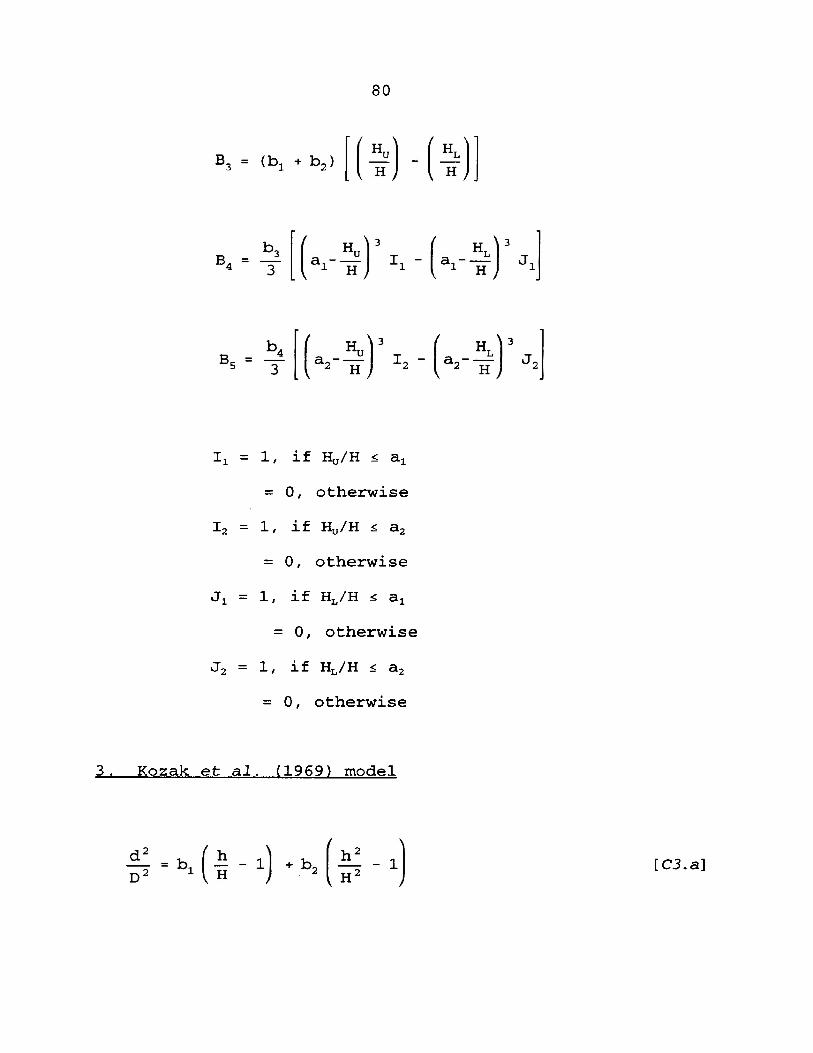
80

11 = 1, if H„/H < ai

= 0, otherwise

12 = 1, if Hu/H ^ 32

= 0, otherwise

Ji = 1, if U^/H < 3i

= 0, otherwise

J2 = 1, if H^/H i 32

= 0, otherwise

3. Kozak et al. (1969) model

[C3.a]

81

h =

(-b,H) - N

(biH)2 - 4b2 (boH^ - d^H-

2 b. [C3.b]

V, {0.0000785D^) bo(H„-Hj 2 H 3 H-

[C3.c]

Where:

bo = -t>i - bj

4. Ormerod's (1973) model

d^ _ I' H-h

D2 ■ i H-1.3j [C4.a]

h = H - (H - 1.3) [C4.b]

VL = (0.00007850^)(H-1.3)

V H-1.3 -( H-1.3 [C4.c]

Where: Y = 2 bi + 1

82

APPENDIX D FORTRAN PROGRAM TO CALCULATE THE WOOD PRODUCT MIXES FOR STAND

This program was written to facilitate the calculations for the wood product mixes based on dbh class distributions of a stand. The input data includes only species, dbh classes and number of stems per dbh class. The output includes: volumes for various wood products for each dbh class and species, and the total for each species and stand. The heights in the program are calculated by the corresponding regional or provincial pooled-site single-entry volxime equations. If site classes are available, the site-stratified single-entry volume equations can be used to calculate the height for each dbh class. Top diameters and section heights in the program are calculated by Max and Burkhart's stem profile equations, while all the volume calculations are made by the stem profile equations by Demaerschalk.

The specifications of wood products were taken from Northern Wood Preservers Inc., Thunder Bay, Ontario. Four types of products were included, i.e., veneer logs, pulp logs, saw logs and chips. Because of the similar dimensional requirements for saw logs and pulp logs, the output of these two products can be assigned either way depending on the product preference. Basically, chips take everything.

Since the dimensional requirements of wood products vary from case to case, and from time to time, minor adjustment is needed according to specific product specifications.

PARAMETERS AND VARIABLES DESCRIPTION

nl

n2 minven maxven minsaw minpulp maxpulp c

stem

niomber of diameter classes for all the species in the stand number of species in the stand minimiam diameter requirement for veneer logs maximum diameter requirement for veneer logs minimiam diameter requirement for saw logs minimum diameter requirement for pulp logs maximum diameter rec[uirement for pulp logs constant in the calculation of log voliome for the metric system number of stems for given dbh class

83

no

sppstem stdstem sppl spp2 dbh ht voltre voids venl sawl pulpl chipl ven2 saw2 pulp2 chip2 dstp hi h2 al a2 bl b2 b3 b4 dl d2 d3 d4 slen

hvmin

hsmin

hpmin

hvmax

hpmax

yvininl

yvmin2

series number assigned to each species in the coefficient file (wood.coe) total stems for given species in the stand total stems for the stand species' name in the stand data file (stand.dat) species' name in the coefficient file (wood.coe) dbh class calculated total height for dbh by Equation [1] calculated tree volume for dbh by Equation [Cl.c] total volume for dbh class average voliime of veneer logs for dbh class average volume of saw logs for dbh class average volume of pulp logs for dbh class average volxime of chips for dbh class total volume of veneer logs for dbh class total volume of saw logs for dbh class total volxime of pulp logs for dbh class total volume of chips for dbh class diameter at stump height coefficient bl in Equation [1] coefficient b2 in Equation [1] upper join point al in Equation [C2.a] upper join point a2 in Equation [C2.a] coefficient bl in Equation [C2.a] coefficient b2 in Equation [C2.a] coefficient b3 in Equation [C2.a] coefficient b4 in Equation [C2.a] coefficient bl in Equation [Cl.a] coefficient b2 in Equation [Cl.a] coefficient b3 in Equation [Cl.a] coefficient b4 in Equation [Cl.a] log lengths requirements of veneer logs, saw logs and pulp logs height limit at minven for the volume calculation of veneer logs height limit at minsaw for the volume calculation of saw logs height limit at minpulp for the volume calculation of pulp logs height limit at maxven for the volume calculation of veneer logs height limit at maxpulp for the volume calculation of pulp logs nvimber of slen for the volume calculation of veneer logs in the case of minimum diameter requirement actual length qualified for the voliame calculation of veneer logs in the case of minimiam diameter requirement

84

yvmaxl

yvmax2

ysminl

ysmin2

ypminl

ypmin2

ypmaxl

ypmax2

stdven stdsaw stdpulp stdchip stdvol wavedbh waveht wavetre sppven

sppsaw

spppulp

sppchip

sppvol waspdbh

waspht

wasptre

number of slen for the volume calculation of veneer logs in the case of maximiom diameter requirement actual length qualified for the volume calculation of veneer logs in the case of maximum diameter requirement number of slen for the volume calculation of saw logs in the case of maximum diameter requirement actual length qualified for the voliome calculation of saw logs in the case of maximum diameter requirement number of slen for the volume calculation of pulp logs in the case of minimum diameter requirement actual length qualified for the volume calculation of pulp logs in the case of minimum diameter requirement number of slen for the volume calculation of pulp logs in the case of maximxam diameter requirement actual length qualified for the volume calculation of pulp logs in the case of maximum diameter requirement total volume of veneer logs for the stand total volume of saw logs for the stand total volume of pulp logs for the stand total volume of chips for the stand total volume for the stand weighted average dbh for the stand weighted average height for the stand weighted average tree voliime for the stand total volume of veneer logs for given species in the stand total volume of saw logs for given species in the stand total volume of pulp logs for given species in the stand total volume of chips for given species in the stand total volume for given species in the stand weighted average dbh for given species in the stand weighted average height for given species in the stand weighted average tree voliome for given species in the stand

85

*** PARAMETER ENTRANCE ***

parameter(nl=74,n2=13,minven=23,maxven=51,minsaw=ll,

$ minpulp=10,maxpulp=41,slen=2.54,c=.0000785)

*** VARIABLE DEFINITION AND STORAGE ALLOCATION ***

character*2 sppl(nl),spp2(n2) integer stem(nl),sppstem(n2),stdstem,no(n2)

real dbh (nl) , ht (nl) , voltre (nl) , voids (nl) , venl (nl) ,

ven2(nl),sawl(nl),saw2(nl),pulpl(nl),pulp2(nl), chipl(nl),chip2(nl),dstp(nl),hvmin(nl),hsmin(nl),

hpmin(nl),hvmax(nl),hpmax(nl),yvminl(nl),

yvmin2 (nl) , yvmaxl (nl) , yvmax2 (nl) , ypminl (nl) ,

ypmin2(nl),ypmaxl(nl),ypmax2(nl),ysminl(nl), ysmin2 (nl) , hi (n2) , h2 (n2) , al (n2) , a2 (n2 ) , bl(n2) ,b2(n2) ,b3(n2) ,b4(n2) ,dl(n2) ,d2(n2) , d3(n2),d4(n2),sppdbh(n2), sppht(n2),spptre(n2),

waspdbh(n2),waspht(n2),wasptre(n2),sppvol(n2), sppven(n2),sppsaw(n2),spppulp(n2),sppchip(n2)

*** OPEN I/O UNITS ***

opend, file= ' stand.dat ‘ , status= 'old' )

open(2,file='wood.coe',status='old')

open(3,file='wood.out',status='new')

*** READ THE STAND FILE AND THE COEFFICIENT FILE ***

do i=l,nl

read(1,*)sppl(i),dbh(i),stem(i)

end do

do i=l,n2

read (2,*)no(i),spp2(i),hi{i),h2(i),al(i),a2(i),

$ bl(i),b2(i),b3(i),b4(i),dl(i),d2(i), $ d3 (i) , d4 (i) end do

86

*** CALCULATE THE VOLUMES FOR VARIOUS PRODUCTS *** *** FOR EACH SPECIES AND DBH CLASS BASED ON ***

*** THE DIMENSIONAL REQUIREMENTS ***

do i=l,nl do k=l,n2

if(sppl(i) .eq. spp2(k))j=no(k) end do ht(i)=1.3+hl(j)*exp(h2(j)/dbh(i) ) voltre(i)=(c*10**(2*dl(j))*dbh{i)**(2*d2(j))*

$ ht(i)**(2*d4(j})*ht(i)**(2*d3(j)+l)) $ /(2*d3(j)+l)

voids (i) =voltre (i) *stem (i) dstp(i)=dbh(i)*sqrt(bl(j)*(0-1)+b2(j)*(0-1)+

$ b3(j)*al(j)**2+b4(j)*a2(j)**2) ddl=dbh(i)*sqrt(bl(j)*(al(j)-1)+

$ b2(j)*(al(j)*al(j)-l)) dd2=dbh(i)*sqrt(bl(j)*(a2(j)-1)+

$ b2(j)*(a2(j)*a2(j)-l)+b3(j)*(al(j)-a2(j))**2) if(sppKi) .eq. 'sb' .or. sppl(i) .eq. ' sW ) then

if(minven .ge. ddl)ivminl=l if(minven .It. ddl)ivminl=0 if(minven .ge. dd2)ivmin2=1 if(minven .It. dd2}ivmin2=0 xvminl=-bl(j)-b2(j)-((minven/dbh(i))**2)+

$ ivminl*al(j)*al(j)*b3(j)+ $ ivmin2 *a2(j)*a2(j)*b4(j)

xvmin2=bl(j)-2 *ivminl*al(j)*b3(j)- $ 2 *ivmin2 *a2(j)*b4(j)

xvmin3 =b2(j)+ivminl*b3(j)+ivmin2 *b4(j) root=xvmin2**2-4*xvminl*xvmin3 hvmin(i)=ht(i)*(-xvmin2-sqrt(root))/(2*xvmin3) if(dstp(i) .It. minven)hvmin(i)=0 yvminl(i)=int(hvmin(i)/slen) yvmin2(i)=yvminl(i)*slen venl(i)=(c*10**(2*dl(j))*dbh(i)**(2*d2(j))*

ht(i)**(2*d4(j))*((ht(i)-0)** (2*d3(j)+l)-(ht(i)-yvmin2(i))** (2*d3(j)+l)))/(2*d3(j)+l)

if(maxven .ge. ddl)ivmaxl=1 if(maxven .It. ddl)ivmaxl=0 if(maxven .ge. dd2)ivmax2=1 if(maxven .It. dd2)ivmax2=0 xvmaxl=-bl(j)-b2(j)-((maxven/dbh(i))**2)+

$ ivmaxl*al(j)*al(j)*b3(j)+ $ ivmax2 *a2(j)*a2(j)*b4(j)

xvmax2=bl(j)-2*ivmaxl*al(j)*b3(j)- $ 2 *ivmax2 *a2(j)*b4(j)

</>-C/> ■(/>

-i/y

•</>■(/>

</>-(/></>

87

xvmax3=b2(j)+ivmaxl*b3(j)+ivmax2 *b4(j) root=xvmax2**2-4*xvmaxl*xvmax3 hvmax(i)=ht(i)*(-xvmax2-sqrt(root))/{2*xvmax3) if(dstp(i) .It. maxven)hvmax(i)=0 yvmaxl(i)=int(hvmax(i)/slen) yvmax2(i)=yvmaxl(i)*slen sawl(i)=(c*10**(2*dl(j))*dbh(i)**(2*d2(j})

*ht(i)**(2*d4(j))*((ht(i)-O)** (2*d3 (j)+l)-(ht(i)-yvmax2(i))** (2*d3(j)+l)))/(2*d3(j)+l)

saw2(i)=sawl(i)*stem(i) venl(i)=venl(i)-sawl{i) ven2(i)=venl(i)*stem(i) if{minpulp .ge. ddl)ipl=l if(minpulp .It. ddl)ipl=0 if(minpulp .ge. dd2)ip2=l if(minpulp .It. dd2)ip2=0 xpminl=-bl(j)-b2(j)-((minpulp/dbh(i))

**2}+ipl*al(j)*al(j)*b3(j)+ ip2 *a2(j)*a2(j)*b4(j)

xpmin2=bl(j)-2*ipl*al(j)*b3(j)- 2*ip2*a2(j)*b4(j)

xpmin3=b2(j)+ipl*b3(j)+ip2*b4(j) root=xpmin2 * *2-4 *xpminl*xpmin3 hpmin(i)=ht(i)*(-xpmin2-sqrt(root))/(2*xpmin3) if(dstp(i) .It. minpulp)hpmin(i)=0 Ypminl(i)=int(hpmin(i)/slen) ypmin2(i)=ypminl(i)*slen pulpl(i) = (c*10**(2 *dl(j))*dbh(i)* *

(2*d2(j))*ht(i)**(2*d4(j))* ((ht(i)-0)**(2*d3(j)+l)-(ht(i)- ypmin2 (i) )**(2*d3(j)+l)))/(2*d3(j)+l)

pulpl(i)=pulpl(i)-venl(i)-sawl(i) pulp2(i)=pulpl(i)*stern(i) chipl(i)=voltre(i)-venl(i)-sawl(i)-pulpl(i) chip2(i)=chipl(i)*stem(i)

else if(sppl(i) .eq. 'pj' .or. sppl(i) .eq. 'pr' $ .or. sppl(i) .eq. 'pw' .or. sppl(i) .eq. $ 'bf')then

if(sppl(i) .ne. 'bf')then if(minpulp .ge. ddl)ipl=l if(minpulp .It. ddl)ipl=0 if(minpulp .ge. dd2)ip2=1 if(minpulp .It. dd2)ip2=0 xpminl=-bl(j)-b2(j)-((minpulp/dbh(i))**2)+

$ ipl*al(j)*al(j)*b3(j)+ $ ip2*a2(j)*a2(j)*b4(j)

xpmin2=bl(j)-2*ipl*al(j)*b3(j)- 2*ip2*a2(j)*b4(j) $

</>-

{/>-

(/>

</V

-t/>

<J><A

</><

/></

>

88

xpmin3=b2(j)+ipl*b3{j)+ip2*b4(j) root=xpmin2 * *2-4 *xpminl*xpmin3 hpmin(i)=ht(i)*{-xpmin2-sqrt(root))

$ /(2 *xpmin3) if(dstp(i) .It. minpulp)hpmin{i)=0 Ypminl(i)=int(hpmin(i)/slen) ypmin2(i)=ypminl(i)*slen pulpl(i) = (c*10*-*^(2*dl(j ) ) *dbh(i) **(2*d2 (j ) )*

ht(i)**(2*d4(j})*((ht(i)-0)** (2*d3(j)+l)-(ht(i)-ypmin2(i))** (2*d3(j)+l)))/(2*d3(j)+l)

if(maxpulp .ge. ddl)ipmaxl=l if(maxpulp .It. ddl)ipmaxl=0 if(maxpulp .ge. dd2)ipmax2=l if(maxpulp .It. dd2)ipmax2=0 xpmaxl=-bl(j)-b2(j)-((maxpulp/dbh(i))**2)+

ipmaxl*al(j)*al(j)*b3(j)+ipmax2 *a2(j)* a2(j)*b4(j)

xpmax2=bl(j)-2*ipmaxl*al(j)*b3(j)- 2*ipmax2*a2(j)*b4(j)

xpmax3=b2(j)+ipmaxl*b3(j)+ipmax2 *b4(j) root=xpmax2 * *2-4 *xpmaxl*xpmax3 hpmax(i)=ht(i)*(-xpmax2-sqrt(root))

/(2 *xpmax3) if(dstp(i) .It. maxpulp)hpmax(i)=0 ypmaxl(i)=int(hpmax(i)/slen) ypmax2(i)=ypmaxl(i)*slen sawl(i)=(c*10**(2*dl(j))*dbh(i)**

(2*d2(j))*ht(i)**(2*d4(j))*((ht(i)-O) **(2*d3 (j)+1)-(ht(i)-ypmax2(i)) **(2*d3(j)+l)))/(2*d3(j)+l)

saw2(i)=sawl(i)*stem(i) pulpl(i)=pulpl(i)-sawl(i) pulp2(i)=pulpl(i)*stem(i) chipl(i)=voltre(i)-pulpl(i)-sawl(i) chip2(i)=chipl(i)*stern (i)

else if(minsaw .ge. ddl)isl=l if(minsaw .It. ddl)isl=0 if(minsaw .ge. dd2)is2=l if(minsaw .It. dd2)is2=0 xsminl=-bl(j)-b2(j)-((minsaw/dbh(i))**2)+

$ isl*al(j)*al(j)*b3(j)+ $ is2*a2(j)*a2(j)*b4(j)

xsmin2=bl(j)-2*isl*al(j)*b3(j)- $ 2*is2*a2(j)*b4(j)

xsmin3=b2(j)+isl*b3(j)+is2*b4(j) root=xsmin2 * *2-4 *xsminl*xsmin3 hsmin(i)=ht(i)*(-xsmin2-sqrt(root))

■(A -(A

-C/

>

89

$ /(2 *xsmin3) if(dstp(i) .It. minsaw)hsmin(i)=0 ysminl(i)=int(hsmin(i)/slen) ysmin2(i)=ysminl(i)*slen sawl(i)=(c*10**(2*dl(j))*dbh(i)

**(2*d2(j))*ht(i)**(2*d4(j))* ((ht(i)-0)**(2*d3(j)+l)-(ht(i)- ysmin2(i) )**{2*d3(j)+l)))/(2*d3(j)+l)

saw2(i)=sawl(i)*stem(i) chipl(i)=voltre(i)-sawl(i) chip2(i)=chipl(i)*stem(i)

end if else

chipl(i)=voltre(i) chip2(i)=chipl(i)*stem(i)

end if do k=1,n2

sppdbh(j)=sppdbh(j)+dbh(i)*stem(i) sppht(j)=sppht(j)+ht(i)*stem(i) spptre(j)=spptre(j)+voltre(i)*stem(i) sppstem(j)=sppstem{j)+stem{i) sppvol(j)=sppvol(j)+volcls(i) sppven(j)=sppven(j)+ven2(i) sppsaw(j)=sppsaw(j)+saw2(i) spppulp(j)=spppulp(j)+pulp2(i) sppchip{j)=sppchip(j)+chip2(i)

end do end do

*** CALCULATE THE SUMMARY INFORMATION FOR EACH SPECIES ***

do k=l,n2 sppdbh{k > =sppdbh{k)/n2 sppht(k)=sppht(k)/n2 spptre(k)=spptre(k)/n2 sppstem(k)=sppstem(k)/n2 sppvol(k)=sppvol(k)/n2 sppven(k)=sppven(k)/n2 sppsaw(k)=sppsaw(k)/n2 spppulp(k)=spppulp(k)/n2 sppchip(k)=sppchip(k)/n2

end do do k=l,n2

if(sppstem(k) .eq. 0)goto 10 waspdbh(k)= sppdbh(k)/spps tem{k) waspht(k)=sppht(k)/sppstem(k)

</></> <A

STAND **

wasptre(k)=spptre(k)/sppstem(k) continue

end do

** CALCULATE THE SUMMARY INFORMATION FOR THE

do i=l,nl stddbh=stddbh+dbh(i)*stem(i) stdht=stdht+ht(i)*stem(i) stdtre=stdtre+voltre(i)*stem(i) stdstem=stdstem+stem(i) stdvol=stdvol+volcls(i) stdven=stdven+ven2(i) stdsaw=stdsaw+saw2(i) stdpulp=stdpulp+pulp2(i) stdchip=stdchip+chip2(i)

end do wavedbh= s tddbh/s tds tem waveht=s tdht / s tds tern wavetre=stdtre/stdstern

*** WRITE THE RESULTS INTO A FILE ***

do i=l,nl write(3,100)sppl(i),dbh(i),ht(i),voltre(i),

$ stem(i) , voids (i) ,ven2 (i) , saw2 (i) , $ pulp2(i),chip2(i) end do write(3,*) write(3,200) write(3,*) do k=l,n2

if(sppstem(k) .eq. 0)goto 20 write(3,100)spp2(k),waspdbh(k),waspht(k),

wasptre(k),sppstem(k),sppvol(k), sppven(k),sppsaw(k),spppulp(k), sppchip(k)

continue end do write(3,*) write(3,300) write(3,*) write(3,400)wavedbh,waveht,wavetre,stdstem,stdvol.

91

$ stdven,stdsaw,stdpulp,stdchip

100 format (lx, lx, a2 , lx, f 6.2, lx, f 5.2, lx, f 7.4 , lx, i5, lx,

$ 5(f8.4,lx)) 200 format(lx,'Sum By Species') 300 format(lx,'Sum For Stand')

400 format(lx, 'ALL',lx,f 6.2,lx,f 5.2,lx,f7.4,lx,i5,lx,

$ 5(f8.4,lx))

*** TERMINATION ***

close(1) close(2)

close(3)

end

92

APPENDIX E PARAMETERS ESTIMATED FOR HEIGHT PREDICTION EQUATIONS FOR NORTHWESTERN ONTARIO

Species Site Class

n bl b2 MSE R^2

BF

BW

CE PB PJ

PO

PR PW SB

SW

X 1 2 X 1 2 3 4

all all X 1 2 3 4 X 1 2 3 4

all all X 1 2 3 4 X 1 2 3 4

707 22 249 18 80 17 54 26

120 22 278 21 205 19 56 14

108 20. 97 30.

126 34. 701 29. 728 24. 289 21. 211 17. 48 37.

304 34. 572 29. 376 24. 82 19.

255 31. 156 36.

1207 31. 843 25. 368 23. 200 20. 67 18. 66 35.

177 28. 160 24. 142 18. 44 19.

.818273263

.716505098

.321345520

.297706997

.702191598

.958976921

.431364659

.988555192

.852090879

.950104918

.632608581

.265315093

.513127228

.514253897

.987117727

.050960011

.086275614

.098611992

.131662518

.125505467

.122271305

.636781025

.982456506

.378487459

.349415943

.603962286

.206273560

.078552868

.241795450 867107680 946863913 080465571

-9.305068218 -8.292207951 -9.208221703 -7.546553657 -6.638045700 -7.198197907 -6.802603434 -6.369777598 -13.28011589 -13.14854045 -13.52132614 -10.74093509 -8.562328324 -8.447308384 -10.14030491 -11.42473368 -10.53863669 -9.037323405 -7.934089579 -7.345334345 -14.89367610 -21.67734865 -13.76392665 -10.80154231 -10.20145156 -8.748798714 -8.438616673 -13.71269628 •11.78307572 ■11.78806361 ■8.501655304 ■11.17130907

3.6691 3.1295 2.3866 8.7855 3.3614 3.2973 2.9670 3.5229 3.8347 6.9557 7.6948 4.2500 2.8267 2.7316

7699 5611 0925 1126 1650 7123

8.9824 12.1348 5.5905 4.4024 3.5258 2.3506 1.9438 8.2368 5.0150 3.7519 3.4997 3.0038

2 6 6 4 4 4

.6959

.6466

.7661

.7258

.7178

.7596

.7626

.3945

.6328

.5594

.7171

.6774

.5984

.5511

.8525

.8651

.7576

.7831

.7434

.5987

.3273

.5569

.7225

.6238

.6282

.5227

.6151

.6154

.7387

.7561

.6676

.5872

93

APPENDIX F PARAMETERS ESTIMATED FOR HEIGHT PREDICTION EQUATIONS FOR NORTHEASTERN ONTARIO

Species Site Class

n bl b2 MSE R^2

AB AT

BF

BW

BY CE

LA MS MR PB PJ

PR PW SB

SW

all 19 27.105310473 X 73 39.848042264 1 436 33.292827450 2 574 29.026879221 3 285 26.020787522 4 36 18.039105995 X 338 24.616877453 1 168 19.237259645 2 82 17.659089963 3 18 14.542580553 X 75 31.007696108 1 220 26.788705122 2 422 22.956840332 3 262 20.391925794 4 44 16.482864837

all 35 23.162540929 X 30 24.238095916 1 112 22.664895451 2 131 19.454985994 3 97 18.042273723 4 22 18.120643850

all 108 27.325001194 all 18 26.566574936 all 76 20.168867613 all 80 27.466417990 X 643 31.334591113 1 1048 24.682442456 2 267 19.848218234 3 68 18.398041518 4 12 12.214712941

all 20 29.193414089 all 144 44.718891012 X 1013 28.911560847 1 643 26.164808352 2 378 22.785412552 3 109 19.653549109 4 27 15.193740215 X 58 39.055819399 1 178 28.148559099 2 143 24.936253768 3 89 22.412100762 4 16 14.630627874

-12.87520504 -12.04180321 -9.971991437 -9.415972261 -9.397394270 -6.174607315 -10.32802211 -9.122497460 -9.395660795 -8.969533426 -9.946290239 -9.022286644 -8.262002419 -8.318052225 -8.906881208 -11.66922779 -13.36555640 -15.62751807 -13.25067820 -13.85980607 -17.46896412 -11.27409620 -14.03096091 -7.312805668 -10.51183997 -10.87619213 -7.574868031 -5.305364509 -7.559071417 -4.893522516 -15.01969211 -25.49728345 -12.41259173 ■11.56642286 -10.22217594 ■8.731535971 ■7.154421233 -18.25027976 -11.82323001 -11.03818561 ■11.71953303 -7.691622550

2 1 3 4

3.2974 9.2977 5.5881 4.4864 4.7240 2.3088 4.0635

1395 6601 1772 8776

3.3678 2.8551 3.1253 1.6473 4.5393 5.4862 3.5584 2.4338 2.3993 1.0230 5.5704 2.5842 4.4292 4.8366 5.7133 5.4309 5.6855 4.8732

9610 5388 4902 5356 9313 1512

1.7093 1.1602 7.7796 2.9828 3.0320 1.8943 1.2442

.6847

.7399

.5993

.5838

.6232

.6081

.6254

.7565

.8095

.6233

.7175

.5974

.5895

.6288

.6834

.4472

.6965

. 6447

.7226

.7483

.8076

.7741

.7850

.5655

.7176

.6461

.5503

.2529

.3166

.2764

.4650

.7969

.6186

.7257

.7284

.8066

.7363

.5077

.5720

.6668

.7970

.7351

94

APPENDIX G PARAMETERS ESTIMATED FOR STEM PROFILE MODELS

Appendix G-1 Parameters estimated for Demaerschalk's (1972) model

Species Size bl b2 b3 b4 MSE R'-2

Largetooth aspen 592 -.049975 Aspen (gen.) 3175 -.043488 Trembling aspen 854 .033251 Beech 114 .029611 Balsam fir 494 .069513 White birch 591 .038528 White cedar 802 .077032 Jack pine 3185 .065070 Red pine 4869 .103114 White pine 5254 .085613 Black spruce 1031 .095149 White spruce 424 .145635

.970239 1.003737 1.035324

047708 016638 020312 063347 970354 958414 985592 015739 000732

0.690464 0.578755 0.662901 0.724240 0.610619 0.824839 0.949528 0.585574 0.650413 0.693985 0.708131 0.919070

-.617293 -.555715 -.718106 -.769283 -.678979 -.847540 -1.057839 -.602582 -.676005 -.732518 -.780004 -1.002816

.00601

.00350

.00461

.00513

.00472

.00988

.01031

.00600

.00733 ,00785 .00839 ,01275

.94483

.95686

.96321

.96582

.95904

.94219

.93136

.94698

.94216 ,93987 .93988 . 92554

Appendix G-2 Parameters estimated for Max and Burkhart’s (1976) model

Species Size al a2 bl b2 b3 b4 MSE R-'2

Large, aspen 592 .73076 .13441 Aspen (gen.) 3175 .79147 .06141 Trembl. aspen 854 .72509 .08659 Beech 114 .80843 .10064 Balsam fir 494 .75000 .06000 White birch 591 .69187 .10679 White cedar 802 .78424 .07237 Jack pine 3185 .84883 .09964 Red pine 4869 .77652 .09197 White pine 5254 .67025 .04547 Black spruce 1031 .71397 .08635 White spruce 424 .68155 .06664

-4.21696 -5.91138

.04174

.48795

.58296

.97912

.80450

.94986 -5.21237 -3.77996 -3.51982 -3.25958

-4

-6 -4. -3 . -3 -4

2.11106 2.96871 1.97654 3.31302 2 .21483 2.00355 1.89441 2.28480 2.55118 1.82266 1.61500 1.58589

-2.19091 -3.26271 -2.11324 -3.35558 -2.47938 -2.07625 -1.47351 -2.42782 -2.89904 -2.28883 -1.88183 -1.36665

9.91985 65.95177 19.20136 31.68926 45.61874 32.14399 144.22722 29.02209 51.80430

301.61778 65.97321 129.72728

.0051

.0028

.0041

.0035

.0046 , 0067 .0056 .0042 .0054 ,0060 .0045 .0086

.95294

.96616

.96710

.97707

.96019

.96106

.96276

.96315

.95708

.95406

.96765

.95013

95

Appendix G-3 Parameters estimated for Kozak et al (1969) model

Species Size bl b2 MSE R-'2

Largetooth aspen 592 -1.535420 .503360 .00607 Aspen (gen.) 3175 -1.196093 .217476 .00356 Trembl. aspen 854 -1.488934 .446002 .00479 Beech 114 -1.800841 .652085 .00502 Balsam fir 494 -1.374381 .313519 .00523 White birch 591 -2.054222 .871360 .00970 White cedar 802 -2.298352 1.086425 .01013 Jack pine 3185 -1.307885 .276449 .00610 Red pine 4869 -1.542600 .445216 .00845 White pine 5254 -1.642996 .534409 .00893 Black spruce 1031 -1.773200 .612695 .00854 White spruce 424 -2.347415 1.083625 .01304

. 94406

. 95619

.96166

.96594

.95447

.94310

.93234

.94601 , 93332 .93158 .93866 , 92352

Appendix G-4 Parameters estimated for Ormerod's (1973) model

Species Size bl MSE R'^2

Largetooth aspen 592 Aspen (gen.) 3175 Trembling aspen 854 Beech 114 Balsam fir 494 White birch 591 White cedar 802 Jack pine 3185 Red pine 4869 White pine 5254 Black spruce 1031 White spruce 424

.760652

.662443

.716617 ,716830 675254 816980 951282 638243 682922 722503 708058 876742

,00816 00554 ,00645 00558 00712 01018 01035 00711 00823 00877 00900 01341

92472 93171 94835 96177 93785 94014 93079 93710 93507 93280 93532 92113

Documents

Production of regional single-entry volume tables and