Embed Size (px)
Citation preview

Louisiana State UniversityLSU Digital Commons
LSU Master's Theses Graduate School
2007
Production data analysis of shale gas reservoirsAdam Michael LewisLouisiana State University and Agricultural and Mechanical College
Follow this and additional works at: https://digitalcommons.lsu.edu/gradschool_theses
Part of the Petroleum Engineering Commons
This Thesis is brought to you for free and open access by the Graduate School at LSU Digital Commons. It has been accepted for inclusion in LSUMaster's Theses by an authorized graduate school editor of LSU Digital Commons. For more information, please contact [email protected].
Recommended CitationLewis, Adam Michael, "Production data analysis of shale gas reservoirs" (2007). LSU Master's Theses. 2066.https://digitalcommons.lsu.edu/gradschool_theses/2066
PRODUCTION DATA ANALYSIS OF SHALE GAS RESERVOIRS
A Thesis
Submitted to the Graduate Faculty in the
Louisiana State University and
Agricultural and Mechanical College
in partial fulfillment of the
requirements for the degree of
Master of Science in Petroleum Engineering
in
The Department of Petroleum Engineering
by
Adam Michael Lewis
B.S., Louisiana State University, 2005
December, 2007

ii
ACKNOWLEDGEMENTS
I would like to thank Louisiana State University for providing me the opportunity to conduct this
research. I would especially like to thank my mentor and advisor Dr. Richard G. Hughes for
guiding me in this research and sharing his knowledge and experience with me. It has been a
wonderful learning opportunity.
I would also like to thank the other members of my committee Dr. Christopher White and Dr.
Julius Langlinais for their guidance and support in completing this work. Finally, I would like to
thank Devon Energy Corporation who were the providers of the data used in this research. I
greatly appreciate all those people who have helped me along the way; this research and this
experience would have been worse off without your support. Thank you.

iii
TABLE OF CONTENTS
ACKNOWLEDGEMENTS....................................................................................................ii
LIST OF TABLES................................................................................................................. .v
LIST OF FIGURES ...............................................................................................................vi
ABSTRACT........................................................................................................................... xi
1. INTRODUCTION………………………………………………………………………..1
1.1. Shale Gas Reservoirs in the U.S. ……………………………………………………1
1.2. Production Data Analysis in the Petroleum Industry………………………………..1
1.3. Project Objectives…………………………………………………………………....2
1.4. Overview of Thesis…………………………………………………………………..2
2. PRODUCTION DATA ANALYSIS LITERATURE REVIEW..................................... ..4
2.1. The Diffusivity Equation.......................................................................................... ..4 2.2. Dimensionless Variables and the Laplace Transform.................................................7 2.3. Type Curves for Single Porosity Systems................................................................ 10 2.4. Arps and Fetkovich..............................................................................................…. 11
2.5. Use of Pseudofunctions by Carter and Wattenbarger............................................... 14
2.6. Material Balance Time by Palacio and Blasingame................................................. 15
2.7. Agarwal..................................................................................................................... 20 2.8. Well Performance Analysis by Cox et al................................................................. 21
3. SHALE GAS ANALYSIS TECHIQUES LITERATURE REVIEW..............................23
3.1. Description of Shale Gas Reservoirs........................................................................ 23 3.2. Empirical Methods…................................................................................................ 23
3.3. Dual/Double Porosity Systems................................................................................. 25 3.4. Hydraulically Fractured Systems.............................................................................. 27 3.5. Dual/Double Porosity Systems with Hydraulic Fractures........................................ 28 3.6. Bumb and McKee..................................................................................................... 30
3.7. Spivey and Semmelbeck........................................................................................... 32 3.8. Summary of Literature Review................................................................................ 32
4. SIMULATION MODELING..........................................................................................34
4.1. Systems Produced at Constant Terminal Rate.......................................................... 34 4.2. Systems Produced at Constant Terminal Pressure.................................................... 47
4.3. Low Permeability Gas Systems................................................................................ 55
5. SIMULATION MODELING OF ADSORPTION…………………………………….. 59
5.1. Adsorption Systems Produced at Constant Terminal Rate………………………... 59
5.2. Adsorption Systems Produced at Constant Terminal Pressure……………………. 66
6. TRIAL CASES….............................................................................................................78

iv
6.1. Simulation Example Well......................................................................................... 78
6.1.1. Analysis as a Single Porosity System with Adsorbed Gas............................. 78 6.1.2. Analysis as a Single Porosity System without Adsorbed Gas........................ 85 6.1.3. Analysis as a Dual Porosity System with Adsorbed Gas................................ 88 6.1.4. Analysis as a Hydraulically Fractured System with Adsorbed Gas................ 91 6.1.5. Analysis as a Dual Porosity Hydraulically Fractured System with
Adsorbed Gas……………………………………………………………….. 93
6.2. Barnett Shale Example Well #1................................................................................ 96
6.2.1. Data and Data Handling..................................................................................96 6.2.2. Analysis as a Single Porosity System..............................................................97 6.2.3. Analysis as a Dual Porosity System................................................................ 100
6.3. Barnett Shale Example Well #2................................................................................ 103
6.3.1. Data and Data Handling..................................................................................103 6.3.2. Analysis as a Single Porosity System..............................................................104 6.3.3. Analysis as a Dual Porosity System................................................................ 106 6.3.4. Stimulation Analysis....................................................................................... 109
7. SUMMARY, CONCLUSIONS, AND RECOMMENDATIONS...................................113
7.1. Summary................................................................................................................... 113 7.2. Conclusions...............................................................................................................113 7.3. Recommendations..................................................................................................... 115
REFERENCES.......................................................................................................................116
NOMENCLATURE……………………………………………………………………….. 119
APPENDIX A……………………………………………………………………………… 121
APPENDIX B……………………………………………………………………………… 124
VITA...................................................................................................................................... 126

v
LIST OF TABLES
Table 1 – Model 1 Dataset ............................................................................................................ 35
Table 2 – Dataset for Model 2....................................................................................................... 38
Table 3 – Values of λ and ω used in Model 2 ............................................................................... 38
Table 4 – Dataset for Model 3....................................................................................................... 43
Table 5 – Dataset for Model 4....................................................................................................... 45
Table 6 – Dataset for Model 5....................................................................................................... 57
Table 7 – Langmuir properties ...................................................................................................... 59
Table 8 – Matching results for dual porosity systems with adsorption......................................... 72
Table 9 – Simulation Example Well Dataset ................................................................................ 79
Table 10 – qd vs. td match results for single porosity system with adsorbed gas .......................... 81
Table 11 – Summary of matching results for single porosity system with adsorbed gas ............. 84
Table 12 – Summary of matching results for single porosity systems without adsorbed gas....... 87
Table 13 – Summary of matching results for dual porosity systems with adsorbed gas. ............. 91
Table 14 – Summary of matching data for hydraulically fractured systems with adsorbed gas... 92
Table 15 – Summary of matching parameters for dual porosity hydraulically fractured systems
with adsorbed gas .......................................................................................................................... 95
Table 16 – Initial Properties for Barnett Shale Example Well #1................................................. 97
Table 17 – Summary of Matching Results for Barnett Shale Example Well #1 ........................ 101
Table 18 – Summary of matching results for Barnett Shale Ex Well #2.................................... 108
Table 19 – Summary of matching results for the first stimulation job performed on Barnett Shale
Ex Well #2................................................................................................................................... 111
vi
LIST OF FIGURES
Figure 1 – Type Curves for a Single Porosity Homogeneous Reservoir from Schlumberger
(1994) ............................................................................................................................................ 11
Figure 2 – Fetkovich Type Curves from Fetkovich, et al. (1987)................................................. 13
Figure 3 – Type Curves for Gas Systems from Carter (1981) ...................................................... 15
Figure 4 – The effect of gas compressibility and gas viscosity on a rate-time decline curve from
Fraim and Wattenbarger (1987) .................................................................................................... 16
Figure 5 – Dimensionless Type Curves from Agarwal (1999) ..................................................... 22
Figure 6 – Cumulative Production plot from Agarwal (1999)...................................................... 22
Figure 7 – Depiction of dual porosity reservoir (after Serra, et al. 1983)..................................... 26
Figure 8 – Type Curves for a Dual Porosity Reservoir showing varying ω from Schlumberger (1994) ............................................................................................................................................ 26
Figure 9 – Type Curves for a Dual Porosity Reservoir showing varying λ from Schlumberger (1994) ............................................................................................................................................ 27
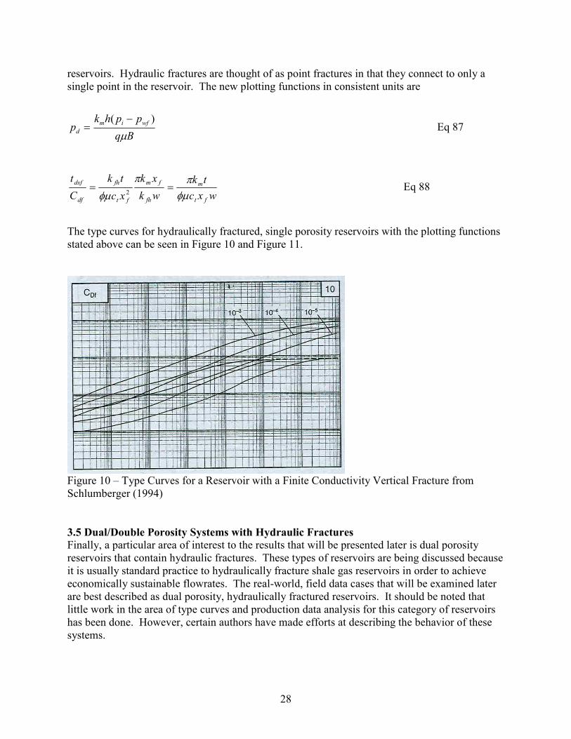
Figure 10 – Type Curves for a Reservoir with a Finite Conductivity Vertical Fracture from
Schlumberger (1994)..................................................................................................................... 28
Figure 11 – Type Curves for a Reservoir with an Infinite Conductivity Vertical Fracture from
Schlumberger (1994)..................................................................................................................... 29
Figure 12 – Type Curves for a Dual Porosity Reservoir with a Finite Conductivity Vertical
Fracture from Aguilera (1989) ...................................................................................................... 30
Figure 13 – Depiction of Model 1................................................................................................. 35
Figure 14 – Wellbore pressure profile for Model 1 ...................................................................... 35
Figure 15 – Diagnostic plot for Model 1 using dimensional plotting functions ........................... 36
Figure 16 – Diagnostic plot for Model 1 using dimensionless plotting functions ........................ 36
Figure 17 – Equivalence of dimensional and dimensionless systems........................................... 37
Figure 18 – Depiction of Model 2................................................................................................. 38
Figure 19 – Wellbore pressure profiles for Model 2 showing the effect of omega ...................... 39
vii
Figure 20 – Diagnostic plot of Model 2 showing the effects of lambda....................................... 40
Figure 21 – Wellbore pressure profiles for Model 2 showing the effects of lambda.................... 41
Figure 22 – Diagnostic plot for Model 2 showing the effects of lambda...................................... 41
Figure 23 – Aerial views of Model 3 ............................................................................................ 43
Figure 24 – Depiction of Model 3................................................................................................. 43
Figure 25 – Wellbore pressure profiles for Model 3 showing the effects of Cdf........................... 44
Figure 26 – Diagnostic plot for Model 3 showing the effects of Cdf ............................................ 44
Figure 27 – Depiction of Model 4................................................................................................. 45
Figure 28 – Wellbore pressure profile for Model 4 showing the effects of fracture half-length .. 46
Figure 29 – Diagnostic plot for Model 4 showing the effects of fracture half-length .................. 47
Figure 30 – Diagnostic plot showing the equivalence of constant rate and constant pressure
derivative curves ........................................................................................................................... 49
Figure 31 -- Diagnostic Plot showing the equivalence of constant rate and pressure systems in a
complex medium........................................................................................................................... 50
Figure 32 -- Rate-decline plot showing the effects of omega ....................................................... 51
Figure 33 – Rate-Decline plot showing the effects of lambda...................................................... 52
Figure 34 – Derivative type curve for constant pressure systems. Shown here converted to an
equivalent constant rate system..................................................................................................... 53
Figure 35 – Rate-Decline type curves for constant pressure systems showing the effects of
dimensionless fracture conductivity.............................................................................................. 54
Figure 36 – Diagnostic plot for a constant pressure system showing the effects of dimensionless
fracture conductivity. Shown here converted to an equivalent constant rate system................... 55
Figure 37 – Rate-Decline type curve showing the effects of changing fracture half-length in a
dual porosity system with a hydraulic fracture. ............................................................................ 56
Figure 38 – Diagnostic plot for a constant pressure system showing the effects of changing
fracture half-length. Shown here converted to an equivalent constant rate system. .................... 57
viii
Figure 39 – Diagnostic plot showing that a shale gas system behaves identically to a “normal”
reservoir on a diagnostic plot ........................................................................................................ 58
Figure 40 – Langmuir isotherm used in simulation models.......................................................... 60
Figure 41 – Wellbore pressure profiles for dual porosity systems showing the effects of
adsorption ...................................................................................................................................... 60
Figure 42 – Diagnostic plot for dual porosity system that shows the effects of adsorption. ........ 61
Figure 43 – Diagnostic plot showing the matching process for adsorbed systems....................... 62
Figure 44 – Wellbore pressure profile for hydraulically fractured systems produced at constant
rate.. ............................................................................................................................................... 64
Figure 45 – Diagnostic plot for hydraulically fractured systems produced at constant rate. ........ 65
Figure 46 – Wellbore pressure profiles for a dual porosity system with a hydraulic fracture ...... 66
Figure 47 – Diagnostic plot for dual porosity systems with a hydraulic fracture ......................... 67
Figure 48 – Rate-decline type curves for dual porosity systems showing the effects of adsorption.
Note that the majority of the effect comes at late-time (i.e. lower pressure). ............................... 69
Figure 49 – Diagnostic plot for constant pressure dual porosity systems..................................... 70
Figure 50 – Diagnostic plot for dual porosity systems with adsorption........................................ 71
Figure 51 – Diagnostic plot for dual porosity systems produced at constant pressure. ................ 72
Figure 52 – Rate-decline type curve for a hydraulically fractured system with adsorbed gas
produced at constant pressure ....................................................................................................... 73
Figure 53 – Diagnostic plot for hydraulically fractured systems with adsorbed gas produced at
constant pressure ........................................................................................................................... 74
Figure 54 – Rate-decline type curve showing the effect of adsorbed gas on dual porosity systems
with hydraulic fractures produced at constant pressure. ............................................................... 75
Figure 55 – Diagnostic plot showing the effects of adsorption on dual porosity systems with
hydraulic fractures produced at constant pressure. ....................................................................... 76
Figure 56 – Depiction of Simulation Example Well Model ......................................................... 79
Figure 57 – Oil-Water Relative Permeability Curve for Simulation Example Well .................... 79

ix
Figure 58 – Gas-Oil Relative Permeability Curve for Simulation Example Well ........................ 80
Figure 59 – Rate Profile for Simulation Example Well ................................................................ 80
Figure 60 – match for qd vs td method for single porosity system with adsorbed gas .................. 82
Figure 61 – match for Fetkovich method for single porosity system with adsorbed gas.............. 83
Figure 62 – match for GPA for single porosity system with adsorbed gas................................... 84
Figure 63 – match results for qd vs. td single porosity system without adsorbed gas ................... 85
Figure 64 – match for Fetkovich method for single porosity systems without adsorbed gas ....... 86
Figure 65 – match for GPA method for single porosity system without adsorbed gas................. 87
Figure 66 – match qd vs. td method for dual porosity systems with adsorbed gas. ....................... 89
Figure 67 – match for Fetkovich method for dual porosity systems with adsorbed gas............... 90
Figure 68 – match for GPA method for dual porosity system with adsorbed gas. ....................... 91
Figure 69 – match using qd vs td for a hydraulically fractured system with adsorbed gas............ 92
Figure 70 – match using GPA for hydraulically fractured system with adsorbed gas.................. 93
Figure 71 – match using qd vs td for a dual porosity hydraulically fractures system with adsorbed
gas.................................................................................................................................................. 94
Figure 72 – match using GPA for dual porosity hydraulically fractured system with adsorbed
gas.................................................................................................................................................. 95
Figure 73 – Combined data plot for Barnett Shale Example Well #1........................................... 98
Figure 74 – Smoothed rate profile for Barnett Shale Example Well #1 ....................................... 99
Figure 75 – Smoothed pressure profile for Barnett Shale Example Well #1................................ 99
Figure 76 – match using GPA for Barnett Shale Example Well #1 assumed to be a single
porosity system with initial pressure of 4000 psi........................................................................ 100
Figure 77 – match using GPA for Barnett Shale Example Well #1 assumed to be a dual porosity
system with initial pressure of 4000 psi. ..................................................................................... 101
Figure 78 – Schematic showing the effects of initial pressure and adsorption parameters ........ 103

x
Figure 79 – Combined data plot for Barnett Shale Ex Well#2 ................................................... 104
Figure 80 – Smoothed rate profile for Barnett Shale Ex Well #2............................................... 105
Figure 81 – Smoothed pressure profile for Barnett Shale Ex Well #2........................................ 105
Figure 82 – match using GPA for Barnett Shale Ex Well #2 assumed to be a single porosity
system with 4000 psi initial pressure. ......................................................................................... 106
Figure 83 – match using GPA for Barnett Shale Example Well #2 assumed to be a dual porosity
system.......................................................................................................................................... 107
Figure 84 – Match using GPA for Barnett Shale Ex Well #2 with an initial pressure of 7500 psi.
..................................................................................................................................................... 109
Figure 85 – Smoothed rate profile for the stimulation job at day 4050 ...................................... 110
Figure 86 – Smoothed pressure profile for the stimulation job at day 4050............................... 110
Figure 87 – match using GPA for the first stimulation job performed on Barnett Shale Ex Well
#2................................................................................................................................................. 111
xi
ABSTRACT
Hydrocarbon resources from unconventional shale gas reservoirs are becoming very important in
the United States in recent years. Understanding the effects of adsorption on production data
analysis will increase the effectiveness of reservoir management in these challenging
environments.
The use of an adjusted system compressibility proposed by Bumb and McKee (1988) is critical
in this process. It allows for dimensional and dimensionless type curves to be corrected at a
reasonably fundamental level, and it breaks the effects of adsorption into something that is
relatively simple to understand. This coupled with a new form of material balance time that was
originally put forth by Palacio and Blasingame (1993), allows the effects of adsorption to be
handled in production data analysis.
The first step in this process was to show the effects of adsorption on various systems: single
porosity, dual porosity, hydraulically fractured, and dual porosity with a hydraulic fracture.
These systems were first viewed as constant terminal rate systems then as constant terminal
pressure systems. Constant pressure systems require a correction to be made to material balance
time in order to apply the correction for adsorption in the form of an adjusted total system
compressibility.
Next, various analysis methods were examined to test their robustness in analyzing systems that
contain adsorbed gas. Continuously, Gas Production Analysis (GPA) (Cox, et al. 2002) showed
itself to be more accurate and more insightful. In combination with the techniques put forth in
this work, it was used to analyze two field cases provided by Devon Energy Corporation from
the Barnett Shale.
The effects of adsorption are reasonably consistent across the reservoir systems examined in this
work. It was confirmed that adsorption can be managed and accounted for using the method put
forth in this work. Also, GPA appears to be the best and most insightful analysis method tested
in this work.
1
1. INTRODUCTION
1.1 Shale Gas Reservoirs in the US
The vast majority of gas production in the United States comes from what are known as
conventional hydrocarbon reservoirs. However, these conventional reservoirs are becoming
increasingly difficult to find and exploit. In an era of rising prices for crude oil and natural gas,
the ability to produce these commodities from unconventional reservoirs becomes very
important. To date, there has been less research done in the area of unconventional gas
production compared to what has been done for conventional gas production.
The term unconventional reservoir requires further explanation. The United States Geological
Survey (USGS) offers a complex definition of which a portion will be presented here. Among
other things, an unconventional reservoir must have: regional extent, very large hydrocarbon
reserves in place, a low expected ultimate recovery, a low matrix permeability, and typically has
a lack of a traditional trapping mechanism (Schenk, 2002).
In particular, shale gas reservoirs present a unique problem to the petroleum industry. They
contain natural gas in both the pore spaces of the reservoir rock and on the surface of the rock
grains themselves that is referred to as adsorbed gas (Montgomery, et al., 2005). This is a
complicated problem in that desorption time, desorption pressure, and volume of the adsorbed
gas all play a role in how this gas affects the production of the total system. Adsorption can
allow for significantly larger quantities of gas to be produced.
Historically, the first commercially successful gas production in the U.S. came from what would
now be considered an unconventional reservoir in the Appalachian Basin in 1821. Currently,
some of the largest gas fields in North America are unconventional, shale gas reservoirs such as
the Lewis Shale of the San Juan Basin, the Barnett Shale of the Fort Worth Basin, and the
Antrim Shale of the Michigan Basin. In addition, gas production from unconventional reservoirs
accounts for roughly 2% of total U.S. dry gas production. (Hill, et al., 2007)
With the world’s, and particularly the U.S.’s, increasing appetite for hydrocarbon based energy
sources, the demand for gas will likely increase. Most experts agree that the days of easy,
conventional gas production are nearly gone. This paves the way for an increase in the gas
production from unconventional reservoirs. As far as the oil industry is concerned, nothing fuels
the desire for more knowledge of a subject quite like an increase in production.
1.2 Production Data Analysis in the Petroleum Industry
For almost as long as oil and gas wells have been produced, there has been some sort of analysis
done on the production data. The main effort has always been, and will continue to be, to
forecast long-term production. Many wells put on production exhibit some sort of decrease in
production over time. Excluding reservoirs with very strong aquifer support, this is due to a
decrease in reservoir pressure. In all cases that will be considered here, this is caused by the
removal of mass (oil or gas) from the reservoir. This decrease in production rate resulted in this
field of petroleum engineering being called decline curve analysis (DCA).

2
Arguably, the first scientific approach to production forecasting was made by Arps (1945). He
developed a set of empirical type curves for oil reservoirs. Little advancement beyond this
empirical method was made until the early 1980’s. Fetkovich (1980) took Arps’ curves and
developed a mathematical derivation by tying them to the pseudosteady state inflow equation. In
doing so, he revolutionized this field of petroleum engineering because the technique presented
showed that there were physical reasons for certain declines which removed much of the
empirical stigma that surrounded DCA. For the first time, an analyst could determine reservoir
properties such as permeability and net pay from an analytical model while having the
confidence that the match to the production data was somewhat unique.
Next, the work of researchers such as Fraim and Wattenbarger (1987) and Palacio and
Blasingame (1993) furthered that of Fetkovich. Fraim and Wattenbarger’s pseudofunctions for
time and pressure accounted for changes gas properties over time; this allowed decline curve
analysis to be rigorously applied to gas reservoirs for the first time. In addition, Palacio and
Blasingame’s development of material balance time allowed for a much more rigorous match to
the production data. Material balance time also allows for constant pressure data to be treated as
constant rate data. This is important because the field of pressure transient analysis (PTA)
emphasizes analytic models for constant rate data. These models are solutions for various
scenarios that are governed by the diffusivity equation. These solutions are much more effective
at identifying flow regimes and reservoir properties than traditional decline curve analysis.
1.3 Project Objectives
Shale gas reservoirs present a unique problem for production data analysis. The effects of the
adsorbed gas are not clearly understood except that it tends to increase production and ultimate
recovery. Lane et al. (1989) presented a methodology based on empirically calculated
adsorption parameters. However, there is no rigorous analytic approach to infer the presence of
adsorbed gas from production data analysis.
That said, this work will outline the effects of adsorbed gas on the common methods of
production data analysis. This will focus on the effect of adsorbed gas on the type curves used
for constant rate and constant pressure production schedules. In addition, the extent to which the
presence of adsorbed gas can be identified with standard production data analysis techniques will
be ascertained.
Lastly, the methods put forth in the work will be applied to a simulated dataset and two datasets
from producing wells in the Barnett Shale. The effects and effectiveness of the methods
presented will be evaluated using these datasets. In addition, what benefit does analyzing
production data as an equivalent well test yield when compared to other analysis methods?
1.4 Overview of Thesis
This first chapter describes the problem that adsorbed gas presents to production data analysis
and why it is necessary to better understand and solve this problem. It also outlines the
objectives of this work.
Chapter 2 is a literature review of production data analysis techniques that are in common use
today. It is intended to serve as refresher of the roots of production data analysis.

3
Chapter 3 is a literature review of shale gas reservoir analysis techniques.
Chapter 4 presents the results of a simulation study that shows the constant rate and constant
pressure type curves for common systems without any effects of adsorbed gas.
Chapter 5 presents the results of a simulation study that shows the effects of adsorbed gas on the
same systems presented in Chapter 4.
Chapter 6 presents 3 example cases, a simulated case and two field cases from the Barnett Shale,
using systems with adsorbed gas. It presents a method for analyzing these systems and the
effects of not treating these systems as adsorbed systems.
Chapter 7 details the conclusions of this work and outlines possible future work in this area.
4
2. PRODUCTION DATA ANALYSIS LITERATURE REVIEW
This literature review is intended to present three overarching concepts. First, there has
been a lot of work done in this area, and most readers will recognize that this review is only a
cursory summary at best. Only the major topics have been covered in an attempt to keep the
discussion flowing. Second, all areas of production data analysis and pressure transient analysis
are connected and very closely related. In reality, these two disciplines of petroleum engineering
are merely working with two different boundary conditions of the same equation. Lastly, there is
room for work to be done regarding the methodology of production data analysis of shale gas
reservoirs.
2.1 The Diffusivity Equation
The roots of production data analysis lie in the diffusivity equation. All production data analysis
makes the assumption that all or part of the production data occurs in boundary-dominated flow.
If this is true, then certain assumptions can be made as to which boundary conditions can be used
to solve the diffusivity equation. To start from the beginning, the diffusivity equation is a
combination of the continuity equation, a flux equation, and an equation of state. The flux
equation used here is Darcy’s Law. For the purposes of this work, the real gas law is used as an
equation of state. This allows for the handling of compressible fluids (i.e. dry gas). Typically,
an exponential relationship between pressure and density is used for cases with small and
constant compressibility, like liquids. The continuity equation and Darcy’s Law are (Lee and
Wattenbarger, 1996)
tr
vr
r
r
∂
∂=
∂
∂−
)()(1 φρρ
Eq 1
r
kvr ∂
Φ∂−=µρ
Eq 2
Assuming that gravity effects are negligible (applicable for an approximately horizontal
reservoir), Darcy’s Law can be re-written as
r
pkvr ∂
∂−=µ
Eq 3
The density term from the real gas law is
z
p
RT
M=ρ
Eq 4
5
Combining the continuity equation, Darcy’s Law, and the real gas law and assuming a
homogeneous medium with constant gas composition and temperature yields (Lee and
Wattenbarger, 1996)
∂∂
=
∂∂
∂∂
z
p
RT
M
tr
pk
z
p
RT
Mr
rrφ
µ1
Eq 5
Assuming permeability and viscosity changes are small and isothermal flow, the equation can be
rearranged and have like terms canceled
∂∂
=
∂∂
∂∂
z
p
tr
p
z
pr
r
k
rφ
µ1
Eq 6
The right hand side of the above equation can be expanded to (Lee and Wattenbarger, 1996)
∂∂
+∂∂
∂∂
=
∂∂
+∂∂
=
∂∂
z
p
pp
z
pt
p
z
p
z
p
ttz
p
z
p
t
φφ
φφφ
φ1
Eq 7
Recalling the definitions of isothermal formation and gas compressibility
∂∂
=p
c fφ
φ1
Eq 8
( )p
zp
p
zcg ∂
∂=
Eq 9
Substituting using the above equations for compressibility
( )gf cct
p
z
p
z
p
t+
∂∂
=
∂∂
φφ
Eq 10
Now, substituting back into the diffusivity equation
t
p
z
p
k
c
t
p
z
p
k
cc
r
p
z
pr
rr
tgf
∂
∂=
∂
∂+=
∂
∂
∂
∂
µφµ
µ
φµ
µ
)(1
Eq 11

6
This is the radial diffusivity equation for a single-phase compressible real gas in a homogeneous,
horizontal medium. In order to solve this equation, it is necessary to treat it like a slightly
compressible fluid. To do this, and retain its applicability to gas reservoirs, the changes in gas
viscosity and compressibility must be taken into account. This is done with the two new
variables called the pseudopressure (m(p)) and the pseudotime (ta) (Lee and Wattenbarger,
1996).
∫=p
pb
dpz
ppm
µ2)(
Eq 12
∫=t
t
itac
dtct
0
)(µ
µ
Eq 13
Substituting these equations into the diffusivity equation yields
at
pm
kr
pmr
rr ∂∂
=
∂
∂∂∂ )()(1 φ
Eq 14
In field units (t in days)
at
pm
kr
pmr
rr ∂
∂=
∂
∂
∂
∂ )(
00634.0
)(1 φ
Eq 15
Now, the above equation is ready to be solved by choosing a set of initial and boundary
conditions. There are many methods and sets of initial/boundary conditions; only a select
number of these solutions will be discussed here. Production data analysis assumes boundary-
dominated flow at a constant bottomhole pressure. This will be discussed later; constant
pressure solutions can also be transformed into constant rate solutions. For this discussion, the
constant rate solution for a well in the center of a cylindrical reservoir will be used. The initial
and boundary conditions are then (in field units) (Lee and Wattenbarger, 1996)
)()0,)(( ipmtrpm ==
Eq 16
sc
sc
rr khT
Tqp
r
pmr
w
50300)(=
∂
∂
=
Eq 17

7
0)(
=
∂
∂
= errr
pm
Eq 18
The approximate, dimensional-space solution to the diffusivity equation with the above
assumptions is (Lee and Wattenbarger, 1996)
−+=∆=−
−
4
3ln
417.1
)(
2)()(
6
w
eg
a
itg
ig
pwfir
r
kh
TqEt
Gzc
pqppmpm
µ
Eq 19
This is a very important solution because it is so similar to some of the solutions used in
production data analysis.
2.2 Dimensionless Variables and the Laplace Transform
The solution to the diffusivity equation presented earlier is a perfectly valid dimensional space
solutions. To solve more complicated systems, certain steps must be taken. To start, the
diffusivity equation for a single-phase compressible fluid in a homogeneous, horizontal medium
is
t
p
k
c
r
pr
rr
t
∂∂
=
∂∂
∂∂ φµ1
Eq 20
A solution to the above equation can be seen in Eq 19. However, a more simple solution exists if
certain variables are created that allow for the simplification of the expressions involved. For
instance, the following equation for pressure has no units, but it encompasses all of the variables
that have an effect on pressure.
Bq
ppkhp
wfi
d µ
)( −=
Eq 21
Dimensionless time and dimensionless radius can also be presented in the same manner.
2
wt
drc
ktt
φµ=
Eq 22
w
dr
rr =
Eq 23
8
The definition of dimensionless variables can mainly be a matter of recognizing the important
groups that govern the equation that is being solved and knowing how to simplify algebraic
expressions. Also, they may be developed from the boundary conditions used for the equations
with the aim of simplifying the resulting solution. In particular, the diffusivity equation sets the
definition of rd and td, while the boundary conditions determine the scaling for pd. Now, using
Eq 23-25, the diffusivity equation can be re-written in dimensionless form as
d
d
d
d
d
dd t
p
r
pr
rr ∂
∂=
∂
∂
∂∂1
Eq 24
with initial condition as
0)( 0 ==dtdd rp
Eq 25
and inner boundary condition (constant-rate production) and outer boundary condition (closed
outer boundary) as
1
1
−=
∂
∂
=drd
d
r
p
Eq 26
0=
∂
∂
= edd rrd
d
r
p
Eq 27
Since, by definition, the dimensionless variables incorporate all of the terms that affect that
variable, most pressure transient plots and production data analysis plots are done using
dimensionless pressure and time variables.
There are many different methods employed to arrive at a solution to the diffusivity equation
with the above boundary conditions. However, a very useful method for solving this
dimensionless equation is by utilizing the Laplace transform. The Laplace transform for
dimensionless pressure is given as (Van Everdingen and Hurst, 1949)
dtetrpsrP dst
ddddd ∫∞
−=0
),(),( Eq 28
where s is the Laplace variable. The diffusivity equation and boundary conditions in Laplace
space are given as
9
d
d
d
dd
d Psdr
Pd
rdr
Pd=+
12
2
Eq 29
sr
P
drd
d 1
1
−=
∂
∂
=
Eq 30
0=
∂
∂
= edd rrd
d
r
P
Eq 31
The solution to Eq 29 with the given boundary conditions in Laplace space is
[ ])()()()(
)()()()(
11112
3
0101
sIsrKsKsrIs
srKsrIsrIsrKP
eded
dedded
d
−
+= Eq 32
with I0 , I1, K0, and K1 being modified Bessel functions of the first and second kind of order 0
and 1. This is the complete form of the analytic solution for a single porosity, homogeneous,
bounded system produced at constant rate. There are many more systems that will be discussed
in this work and their solutions were arrived at in a similar manner as this one. However, one
extremely useful attribute of solutions in Laplace space is the manner in which solutions with
terminal constant pressure boundaries (instead of constant rate) are obtained. In Laplace space,
the relationship between pressure and rate is given as (Van Everdingen and Hurst, 1949)
QsP
2
1= Eq 33
In Eq 33, P is the cumulative pressure drop (i.e. the change in reservoir pressure) in Laplace
space while Q is the cumulative production due to a constant rate in Laplace space. Constant
rate solutions to the diffusivity equation are almost ubiquitous in the petroleum industry. The
definition in Eq 33 implies that the constant pressure solution for any system with a constant rate
solution can be obtained by mere algebra thanks to the Laplace transform.
These solutions are relatively useless if left in Laplace space. The most common method in use
within the petroleum industry is to numerically invert the Laplace space solution using the
Stehfest algorithm one version of which is (Stefhest, 1970)
10
∑
+=
++
−−
−
−=
iN
iF
N
iN
i
iFFiFFN
FFV
,2
max
2
1 2
12
2
)!2()!()!(!2
)!2()1( Eq 34
where Vi is the Stehfest coefficient and N is the Stehfest number. For the solutions considered in
this work, Stehfest numbers between 8 and 12 yield the most stable results.
2.3 Type Curves for Single Porosity Systems
Now, let us examine a specific case that is commonly analyzed in both pressure transient
analysis and production data analysis. It becomes clear why so much effort was spent in
describing the origins of the diffusivity equation in detail, since the analysis of the various
commonly encountered reservoirs almost entirely relies upon type curves. A type curve can be
created for any situation for which an all encompassing, or general solution can be obtained.
These solutions all come from the diffusivity equation and differ only in the assumptions they
make as to the system structure, boundary conditions, and the dimensionless groups chosen.
For instance, a very common solution is the single porosity, slightly compressible liquid type
curves (Eq 32). They use the same pd and td given in Eq 21 and Eq 22, and they include a
dimensionless wellbore storage term given as (Lee and Wattenbarger, 1996)
2
wt
dhrc
CC
φ=
Eq 35
where, for wellbores containing only a single fluid
wellwell cVC *=
Eq 36
and cwell is the compressibility of fluid in the wellbore. In pressure transient analysis, type curves
are typically displayed two ways. First, the dimensionless pressure is plotted against
dimensionless time. Second, a diagnostic plot (i.e. derivative plot) is made. For this case, the y-
axis will be ))()ln(( ddddd CtdpdCt and the x-axis will be td/Cd. The derivative plot allows
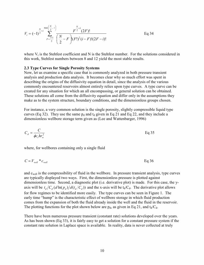
for flow regimes to be identified more easily. The type curves can be seen in Figure 1. The
early time “hump” is the characteristic effect of wellbore storage in which fluid production
comes from the expansion of both the fluid already inside the well and the fluid in the reservoir.
The plotting functions for the plot shown below are pd, as given in Eq 21, and td/Cd.
There have been numerous pressure transient (constant rate) solutions developed over the years.
As has been shown (Eq 33), it is fairly easy to get a solution for a constant pressure system if the
constant rate solution in Laplace space is available. In reality, data is never collected at truly

11
Figure 1 – Type Curves for a Single Porosity Homogeneous Reservoir from Schlumberger
(1994)
constant rate or constant pressure. There are always variations. The data, whether constant rate
or pressure, must be re-initialized at each change. With constant rate data, this is done only with
the time function and is known as superposition. With constant pressure data, re-initialization
must be done in both rate and time and the superposition calculations are more difficult.
Until recently, production data analysis has relied on more empirical methods/solutions because
of the difficulty of analytic solutions. In the last decade, the more rigorous constant pressure
solutions have begun to make a comeback. Building on the success of Fetkovich’s decline
curves, much of the credit for this goes to research groups at Texas A&M University and Fekete
Associates in Canada. Fekete has developed numerous software tools that allow users to access
the analytical constant pressure solutions in the same way pressure transient analysts have done
for years. This combined with high-resolution production data that has historically been
available only for pressure transient testing has breathed new life into production data analysis.
2.4 Arps and Fetkovich
Fetkovich’s main advancement to the area of DCA was to place it on firm
mathematical/theoretical ground. All DCA is in some way based on Arp’s original set of type
curves. These curves were completely empirical and had been regarded as non-scientific. Arps'
decline equation is (Arps, 1945)
bi
i
tbD
qtq
1
)1(
)(
+
=
Eq 37
where the empirical relationship for Di is

12
pi
i
iN
qD = Eq 38
Npi is the cumulative oil production to a hypothetical reservoir pressure of 0 psi. The Arps
equation yields an exponential decline when b = 0 (b = 1 is hyperbolic decline) with an exponent
of –Di*t. The value of b can be indicative of the reservoir type and drive mechanism. Anything
over 0.5 is usually considered multi-layered or heterogeneous. It should be noted that surface
facilities can affect the b value as well. Backpressure on a well will result in a higher b value
than would otherwise be obtained. (Fetkovich et al., 1987)
Hurst (1943) proposed solutions for steady-state water influx. Using modified versions of these
solutions for finite water influx, Fetkovich (1980) proposed that
pi
i
N
tq
wfi
e
ppJtq
)*(
)()(
−= Eq 39
where
ii pqJ /= Eq 40
and
B
hpcrrN itwe
pi615.5
)( 22 φπ −= Eq 41
Assuming that pwf = 0 (wide open decline), one arrives at Arps’ (1945) equation which is
tN
q
i
pi
i
eq
tq −
=)(
Eq 42
So, Fetkovich rederived Arp’s equation and then merged that with pseudosteady-state inflow
equations. So Di = qi / Npi and tDd = (qi / Npi) * t. Assuming a circular reservoir and
pseudosteady inflow, Fetkovich (1980) proposed that
−
Β
−=
5.0ln2.141
)(
w
e
wfi
i
r
r
ppkhq
µ
Eq 43

13
−
−
=
5.0ln15.0
00634.
2
2
w
e
w
e
wtDd
r
r
r
r
rc
kt
tφµ
Eq 44
with qDd = q(t) / qi
−
=
−
Β
−= 5.0ln
5.0ln2.141
)(
)(
w
e
d
w
e
wfi
Ddr
rq
r
r
ppkh
tq
q
µ
Eq 45
where qd is the dimensionless flowrate given by
)(
2.141
wfi
dppkh
quBq
−=
Plotting qDd vs. tDd yields the classic Fetkovich decline curve plot which can be seen in Figure 2.
Figure 2 – Fetkovich Type Curves from Fetkovich, et al. (1987)

14
Fetkovich combined the constant pressure solution to the diffusivity equation with the Arps
equation in a consistent manner which allows a relatively simple, single type curve to be
developed.
Fetkovich never shows the full derivation of his solution. Ehlig-Economides and Joseph (1987)
presented the full derivation of the solution. They also showed that the 0.5 term in Eq 45-47
should be 0.75 considering that this is a pseudosteady-state solution. They also stated that 0.5
appeared to be a better fit to field data even though it is not theoretically correct.
Another important concept introduced to DCA by Fetkovich was re-initialization. Any time the
flow regime changes (for instance, if the well is shut-in, cut back, or stimulated), the production
data must be re-initialized in time and rate. This is done by changing the reference pi and qi and
resetting the time to 0.
2.5 Use of Pseudofunctions by Carter and Wattenbarger
Fetkovich’s decline curves were developed for liquid systems. Carter (1981) recognized that the
assumption of small and constant compressibility was very inaccurate for gas reservoirs
produced at a high drawdown pressure. He developed a variable (γg) that qualified the
magnitude of the error being made when analyzing a gas system using the decline curves for a
liquid system. Carter (1981) defined γg as
wfi
wfigigi
cartzpzp
pmpmc
)/()/(
)()(
2 −
−=µ
λ Eq 46
Where µgi and cgi are the gas viscosity and compressibility at the initial pressure and gµ and gc
are evaluated at average reservoir pressure. Each value of λcart had its own set of decline curve
stems. This is a rather empirical approach that allowed gas systems to plot on liquid system
decline curves. An example of Carter’s decline curves can be seen in Figure 3.
The next significant advancement in DCA came from Fraim and Wattenbarger (1987). Drawing
on concepts from pressure transient analysis and earlier work done by Fetkovich (1980) and
Carter (1981), they introduced the concept of pseudotime for analyzing gas well production data.
Fraim and Wattenbarger (1987) derived the following equation for bounded, radial, gas
reservoirs:
∫−
=
t
gg
igg
igg
ig
i
dtc
c
cG
zp
J
q
q
0
)(
)(
)(2ln
µ
µ
µ
Eq 47
where
Tp
T
rC
A
hkEJ
sc
sc
wA
g
g
=
−
2
5
2458.2ln5.0
9875.1 Eq 48

15
Figure 3 – Type Curves for Gas Systems from Carter (1981)
The shape factor (CA) used in the equation for Jg is 19.1785 rather than the 31.62 for a circular
reservoir. This is done in order to conform to Fetkovich’s type curves. The need for a
pseudotime function is evident after examining Eq 47. Fraim and Wattenbarger (1987) define it
as:
∫=t
t
itac
dtct
0
)(µ
µ
Eq 49
The difference between pseudotime and actual time can be seen in Figure 4 from Fraim and
Wattenbarger (1987). Now, any homogeneous, closed, gas reservoir will exhibit exponential
decline when plotted with the pseudotime function.
2.6 Material Balance Time by Palacio and Blasingame
Palacio and Blasingame (1993) presented the use of material balance time functions to minimize
the effects of variable rate/pressure production histories on the accuracy of DCA forecasts. All
previous methods of DCA required that the well being analyzed be in pseudosteady state
(constant pressure/rate production) in order to isolate the correct transient and decline stems.
Their equation for liquid decline was:
DdwAwfi
o
trCe
A
khpp
q
+=
Β− 1
14ln5.0
2.1412γ
µ Eq 50
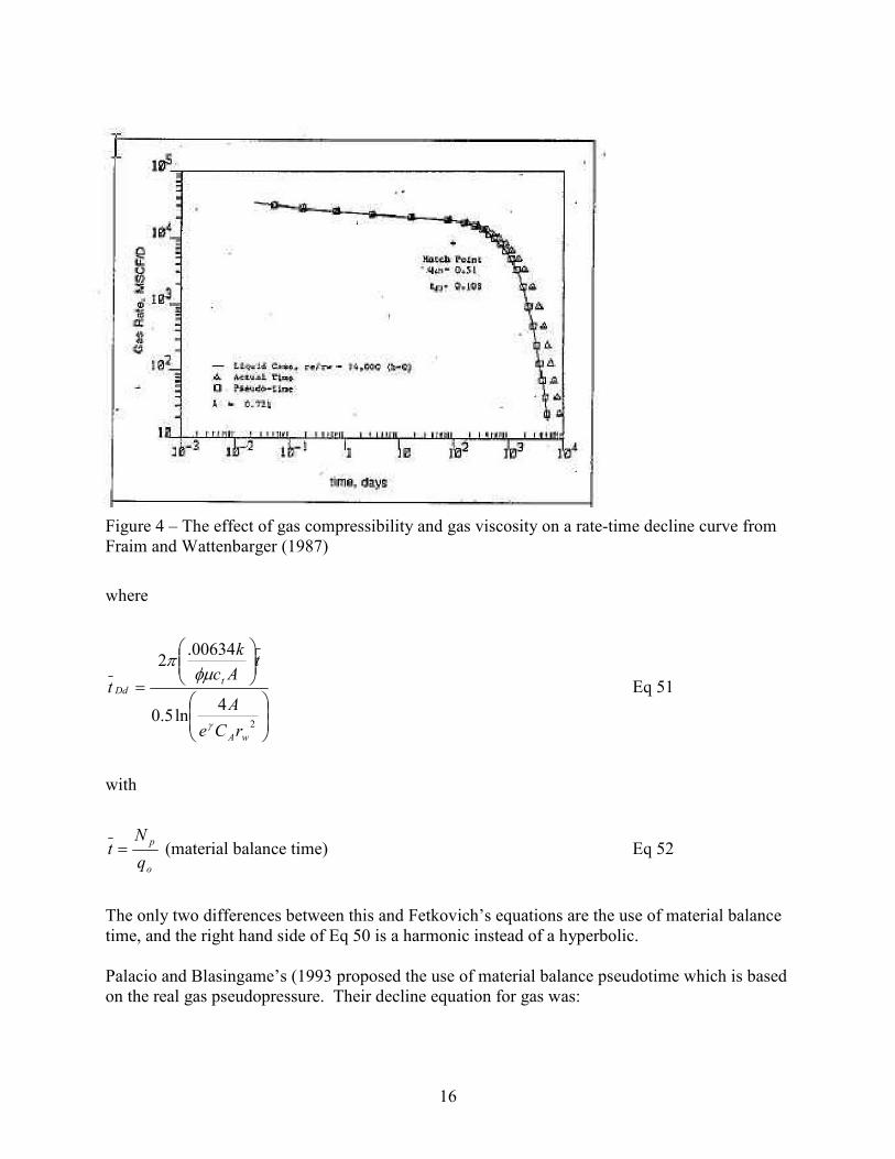
16
Figure 4 – The effect of gas compressibility and gas viscosity on a rate-time decline curve from
Fraim and Wattenbarger (1987)
where
=
2
4ln5.0
00634.2
wA
tDd
rCe
A
tAc
k
t
γ
φµπ
Eq 51
with
o
p
q
Nt = (material balance time) Eq 52
The only two differences between this and Fetkovich’s equations are the use of material balance
time, and the right hand side of Eq 50 is a harmonic instead of a hyperbolic.
Palacio and Blasingame’s (1993 proposed the use of material balance pseudotime which is based
on the real gas pseudopressure. Their decline equation for gas was:
17
aa
g
ptm
q
p=
∆ Eq 53
where
ti
aGc
m1
=
Eq 54
The pseudosteady-state inflow equation is as follows
=
−2
4ln
2
12.141
)()(
wAg
gigi
g
i
rC
A
ehk
B
q
pmpmγ
µ
Eq 55
Adding Eq 54 and Eq 55 gives Palacio and Blasingame’s (1993) coupled decline equation as
a
pssa
a
pssag
i tb
m
bq
pmpm
,,
1)()(
+=−
Eq 56
where
=
2,
4ln
2
12.141
wag
gigi
pssarC
A
ehk
Bb
γ
µ
Eq 57
pTz
zTpB
scsc
scg =
Eq 58
Now, Palacio and Blasingame’s (1993) equation can be re-written as
a
ti
g
wAg
gigi
g tGc
q
rC
A
ehk
Bqpm +
=∆
2
4ln
2
12.141)( γ
µ
Eq 59
While it does not look exactly the same as the solution to the diffusivity equation that was
presented earlier, it is equivalent if you consider that the natural log term in Palacio and
Blasingame’s equation is the more shape factor. The approximation for a well in the middle of a
cylindrical reservoir is ln(re/rw-3/4).
18
Now, it is necessary to examine the decline portion of Eq 59 to elaborate on Palacio and
Blasingame’s approach and their derivation of material balance pseudotime. As was previously
mentioned, the decline equation for gas as presented by Palacio and Blasingame (1993) is
a
tg
tGcq
pm 1)(=
∆
Eq 60
For gas reservoirs, this equation is valid when the pseudotime (ta) includes a material balance
component given as
∫==t
tg
g
g
tigiaa dt
c
q
q
ctt
0µ
µ Eq 61
(material balance incorporated into ta). Pseudopressure is taken as
∫=p
g
dpz
ppm
0
2)(µ
Eq 62
Explaining the derivation of material balance pseudotime requires the use of the gas material
balance equation. This is a well known and widely used relationship between gas production,
corrected reservoir pressure, and original gas in place. The equation for gas material balance
assumes that the reservoir has a closed outer boundary (i.e. is volumetric with no water influx).
Also, the only energy from the reservoir that drives gas production comes from the expansion of
the gas itself. Rock and connate water expansion/compressibility are assumed negligible. The
gas material balance equation under these assumptions is
−=
i
i
pp
z
z
pGG 1
Eq 63
Where Gp = cumulative gas production, and the original gas in place, G, is given by
g
wb
B
SVG
)1( −=
φ Eq 64
For the purposes of this development, gas production rate is more important than cumulative
production. So, the derivative of the gas material balance equation will yield the flowrate. This
expression is then

19
−==
z
p
dt
d
p
zG
dt
dGq
i
ip
g
Eq 65
Rewriting the gas material balance equation
( )t
p
pd
zpd
p
zGq
i
ig ∂
∂−=
Eq 66
Substituting the definition of gas compressibility (Eq 9) into the material balance equation
dt
pdc
z
p
p
zGq g
i
ig −=
Eq 67
Now, this definition of qg can be substituted into the expression for at (Eq 63). The result is
∫
−=
t
tg
g
i
i
g
tigia dt
dt
dp
c
c
z
p
p
Gz
q
ct
0µ
µ
Eq 68
To make this integral easier to solve, Palacio and Blasingame (1993) suggested that, consistent
with the assumptions in gas material balance, the compressibility could be removed by assuming
that gas compressibility (cg) is roughly equal to total system compressibility (ct). This is can be
seen in the equation for system compressibility of a dry gas reservoir below.
fwwgwt ccScSc ++−= )1(
Eq 69
Water compressibility is typically around 1x10⁻⁶ and formation compressibility is typically
around 4 x 10⁻⁶ in consolidated formations. Both of these are 2 to 3 orders of magnitude smaller
than typical values of gas compressibility, even at high pressure. Thus, under these conditions ct
≈ cg and the equation for material balance time can be re-written as
∫
−=
p
p gi
i
g
tigia
i
dpz
p
p
Gz
q
ct
µ
µ
Eq 70
The integral term in this equation is an expression for the real gas pseudopressure difference. So,
the final equation for gas material balance pseudotime is

20
[ ])()(2
pmpmp
Gz
q
ct i
i
i
g
tigia −
=µ
Eq 71
The use of pseudopressure is extremely important when dealing with gas reservoirs because it
accounts for changes in gas viscosity and compressibility, especially if there is a significant
change in reservoir pressure over time. This is the most accurate means of accounting for these
changes in gas properties (Wattenbarger and Lee, 1996).
2.7 Agarwal
The most significant contribution of Agarwal et al. (1999) was their verification of the Palacio
and Blasingame (1993) development of material balance time. Agarwal et al. (1999) used a
single-phase reservoir simulator to compare constant rate and constant pressure systems. They
verified that any system produced at constant pressure could be converted to an equivalent
constant rate system using the material balance time transformation. This is a very important
finding because now the vast library of well known analytical solutions for constant rate systems
can be utilized in production data analysis. In addition, the concept of re-initialization of
production data is much more simple in a constant rate system than in a constant pressure
system.
Agarwal et al. (1999) also made a significant contribution with the use of derivatives in type
curve analysis to greatly aid in the identification of the transition between the transient and
pseudosteady state flow regimes. They used the Palacio and Blasingame (1993) method of
calculating dimensionless adjusted time (taD), which is identical to that of Palacio and
Blasingame (1993) (Eq 69). They also developed their own function of dimensionless time
based on area (tDA).
)(2
A
rtt waDDA = Eq 72
Agarwal et al. (1999) modified three varieties of type curves: rate-time, rate-cumulative
production, and cumulative production-time. Their plot of rate-time is made with 1/pwd vs. tDA.
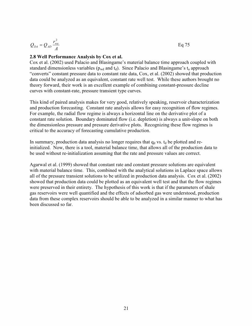
They also plot pwd’ vs. tDA and 1/dln(pwd’) vs. tDA. As is seen in Figure 5, pwd’ has a slope of 2 in the transient period and a slope of 0 during pseudosteady state. This makes it fairly easy to
identify flow regimes when analyzing production data. The Agarwal et al. (1999) equation for
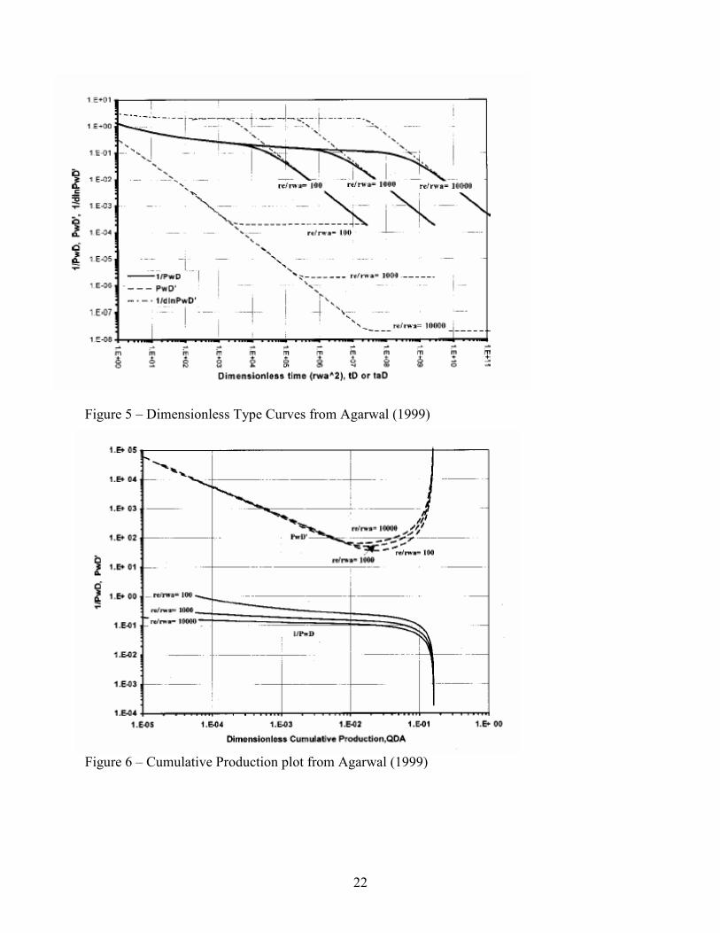
pwd and dimensionless cumulative production (QDA) are
)]()([*
)(14221
wfiwd pmpmkh
tTq
p −= Eq 73
)()(
)()(2002
BHPi
i
iwa
ii
ADpmpm
pmpm
phr
GTzQ
−
−=φ
Eq 74
21
A
rQQ wa
ADDA
2
= Eq 75
2.8 Well Performance Analysis by Cox et al.
Cox et al. (2002) used Palacio and Blasingame’s material balance time approach coupled with
standard dimensionless variables (pwd and td). Since Palacio and Blasingame’s ta approach
“converts” constant pressure data to constant rate data, Cox, et al. (2002) showed that production
data could be analyzed as an equivalent, constant rate well test. While these authors brought no
theory forward, their work is an excellent example of combining constant-pressure decline
curves with constant-rate, pressure transient type curves.
This kind of paired analysis makes for very good, relatively speaking, reservoir characterization
and production forecasting. Constant rate analysis allows for easy recognition of flow regimes.
For example, the radial flow regime is always a horizontal line on the derivative plot of a
constant rate solution. Boundary dominated flow (i.e. depletion) is always a unit-slope on both
the dimensionless pressure and pressure derivative plots. Recognizing these flow regimes is
critical to the accuracy of forecasting cumulative production.
In summary, production data analysis no longer requires that qd vs. td be plotted and re-
initialized. Now, there is a tool, material balance time, that allows all of the production data to
be used without re-initialization assuming that the rate and pressure values are correct.
Agarwal et al. (1999) showed that constant rate and constant pressure solutions are equivalent
with material balance time. This, combined with the analytical solutions in Laplace space allows
all of the pressure transient solutions to be utilized in production data analysis. Cox et al. (2002)
showed that production data could be plotted as an equivalent well test and that the flow regimes
were preserved in their entirety. The hypothesis of this work is that if the parameters of shale
gas reservoirs were well quantified and the effects of adsorbed gas were understood, production
data from these complex reservoirs should be able to be analyzed in a similar manner to what has
been discussed so far.
22
Figure 5 – Dimensionless Type Curves from Agarwal (1999)
Figure 6 – Cumulative Production plot from Agarwal (1999)
23
3. SHALE GAS ANALYSIS TECHIQUES LITERATURE REVIEW
As was mentioned earlier, unconventional reservoirs are playing a larger and larger role in
supplying the demand for hydrocarbons in the United States. In particular, the Barnett shale
formations of the Fort Worth Basin have shown increasing promise in recent years. It is
estimated that the Barnett Shale could contain as much as 250 TCF of gas originally in place.
Ultimate recoveries range from 10 to 20 percent. (Montgomery et al., 2005)
3.1 Description of Shale Gas Reservoirs
Shale gas reservoirs present numerous challenges to analysis that conventional reservoirs simply
do not provide. The first of these challenges to be discussed is the dual porosity nature of these
reservoirs. Similar to carbonate reservoirs, shale gas reservoirs almost always have two different
storage volumes for hydrocarbons, the rock matrix and the natural fractures (Gale et al., 2007).
Because of the plastic nature of shale formations, these natural fractures are generally closed due
to the pressure of the overburden rock (Gale et al., 2007). Consequently, their very low, matrix
permeability, usually on the order of hundreds of nanodarcies (nd), makes un-stimulated,
conventional production impossible. Therefore, almost every well in a shale gas reservoir must
be hydraulically stimulated (fractured) to achieve economical production. These hydraulic
fracture treatments are believed to re-activate and re-connect the natural fracture matrix (Gale et
al., 2007).
Another key difference between conventional gas reservoirs and shale gas reservoirs is adsorbed
gas. Adsorbed gas is gas molecules that are attached to the surface of the rock grains
(Montgomery et al., 2005). The nature of the solid sorbent, temperature, and the rate of gas
diffusion all affect the adsorption (Montgomery et al., 2005). Currently, the only method for
accurately determining the adsorbed gas in a formation is through core sampling and analysis.
The amount of adsorbed gas is usually reported in SCF/ton of rock or SCF/ft3 of rock.
Depending on the situation, adsorbed gas can represent a large percentage of the gas in place and
can have a dramatic impact on production.
3.2 Empirical Methods
Previous efforts of production data analysis of shale reservoirs have focused on identifying the
presence of adsorption/desorption and determining the correct plotting parameters necessary to
accurately estimate reservoir parameters. Lane and Watson (1989) used various types of
numerical simulation models (single porosity with and without adsorption, and dual porosity
with and without adsorption) to attempt to identify adsorption parameters. In addition, they
attempted to determine which type of model gave the best results. They performed a history
match to production data for each type of model. Based on which model yielded the best
statistical match to the production data, they were able to determine whether or not the
desorption mechanism was present.
However, they noted that the shape of the Langmuir isotherm greatly affected their ability to
identify desorption. A linear isotherm indicates very little gas is adsorbed onto the surface of the
shale grains; a non-linear, highly curved, isotherm indicates that large quantities of gas are
adsorbed. In the case of a linear isotherm, the models without desorption were not significantly
different from those with desorption.
24
Lane and Watson (1989) noted that estimating the values of the desorption parameters (and the
Langmuir isotherm) accurately from production data was not possible, but they were able to
accurately determine permeability. However, they stated that if certain reservoir parameters
were independently known, the error in estimating desorption parameters would be greatly
reduced.
Hazlett and Lee (1986) focused on finding an appropriate correlating parameter (plotting
function) for shale gas reservoirs. They correctly noted that the early and intermediate time flow
in dual porosity systems is dominated by the fracture system. Thus, λ, the interporosity flow
coefficient, plays no role. During late time, λ plays a major role while ω, the storativity ratio,
plays only a minor role. So, the approximate solutions to the dual porosity analytical model are:
Early time:
2
1
)(d
dt
qπω
=
Eq 76
Intermediate time:
−−=
)75.0(ln
2exp
75.0ln
12
eDeD
d
eD
drr
t
rq Eq 77
Late time:
−
−−=
)1(
)(exp
2
)1( 2
ωλλ deD
d
trq Eq 78
They also developed new versions of the plotting variables qd and td. Their versions include the
parameter 2
eDrλ , q is replaced with Np/t , and rw is replaced with re. This yields:
)(
)1(894.0
2
wfiet
gp
Drepphrc
BNQ
−
−=φ
ω
Eq 79
and
2
)1(00634.0
etg
Drerc
ktt
φµω−
= Eq 80
When, QDre/tDre is plotted against tDre, an average rate versus time is seen instead of an
instantaneous rate versus time. Hazlett and Lee (1986) noted that accurate values can be

25
determined for the product k x h. However, they showed that the match generated by their
method was not unique for any value of λ, ω, or re.
The methods mentioned do not attempt to characterize the system with any of the known
reservoir models that have analytical solutions. As was stated earlier, the early attempts were
mostly empirical. However, the character of shale gas reservoirs is believed to be known; they
are naturally fractured reservoirs that generally have wells that have been hydraulically fractured
to increase production rate. They have very low matrix permeability and generally contain
adsorbed gas. This forthcoming discussion will outline what analytical models are available that
are similar to shale gas systems. These models can potentially be used in production data
analysis of shale gas reservoirs.
3.3 Dual/Double Porosity Systems
Earlier, analytical type curves for single porosity systems were discussed. Now, a more
complicated solution, the dual porosity reservoir will be examined as it applies better to shale gas
systems. Unless it is otherwise stated, dimensionless time and pressure are those defined in Eq
21 and Eq 22. Here it is necessary to assume several more variables that describe the more
intricate interactions between the naturally occurring fractures in the reservoir and the matrix
rock. Essentially, these reservoirs are treated as two reservoirs, the fractures and the matrix.
The first of these variables is the interporosity flow coefficient (λ) (Gringarten, 1984). This describes how well the natural fractures are connected to one another and to the matrix rock
itself.
f
wm
k
rk2α
λ = Eq 81
where
2
)2(4
mL
nn +=α
Eq 82
where n is the number of normal (90o to one another) fracture planes in the reservoir. For
horizontal fractures or multilayered reservoirs, this number is 1. The maximum value for n is 3
(x, y, and z directions). Lm is the commonly referred to as the characteristic fracture spacing. A
visual depiction is given in Figure 7. (Gringarten, 1984)
The next variable important to dual porosity reservoirs is the storativity coefficient (ω) (Gringarten, 1984). In essence, it compares how large the fracture storativity is in relation to the
total storativity of the reservoir.
mtft
ft
cc
c
)()(
)(
φφ
φω
+=
Eq 83

26
This reservoir depiction is for n = 1.
Figure 7 – Depiction of dual porosity reservoir (after Serra, et al. 1983)
Both λ and ω are dimensionless. The dimensionless plotting functions are slightly different for dual porosity systems when compared to those of single porosity systems. Permeability is now
taken as fracture permeability since that number is usually significantly higher and has more
impact on production performance. Also, total system compressibility and total system porosity
must now incorporate the fractures.
tmtft ccc +=
Eq 84
mft φφφ += Eq 85
The effects of ω and λ on pressure transient type curves with the new plotting functions can clearly be seen in Figure 8 and Figure 9.
Figure 8 – Type Curves for a Dual Porosity Reservoir showing varying ω from Schlumberger (1994)
Matrix
Fracture
hm = Lm
hf
Matrix
Fracture
Matrix

27
Figure 9 – Type Curves for a Dual Porosity Reservoir showing varying λ from Schlumberger (1994)
Figure 8 and Figure 9 clearly show that early time is dominated by the flow from the fractures
themselves. This can be seen in the effects of changing the value of ω. The larger the dips seen in Figure 8 represent decreasing fracture storativity. Intermediate time is dominated by flow
from the matrix into the fractures. This is controlled by the interporosity flow coefficient λ. Figure 9 shows that decreasing fracture-matrix connectivity delays the onset of the effects of ω. In late time, the system behaves like a single porosity system and would exhibit either boundary-
dominated flow (unit-slope) or infinite-acting flow.
3.4 Hydraulically Fractured Systems
Man-made hydraulic fractures are often used in reservoirs that have low permeability that is not
capable of economic production rates. These are very different in character to the naturally
fractured reservoirs that are classified as having a dual/double porosity. Hydraulic fractures are
generally characterized by three variables: fracture half-length xf, fracture width w, and fracture
permeability kfh. These three variables make up the dimensionless fracture conductivity which is
given by (Lee and Wattenbarger, 1996)
fm
fh
dfxk
wkC
π=
Eq 86
Unlike natural fractures, hydraulic fractures are almost entirely vertical in that they cut through
the thickness of a reservoir, and they are typically small in length when they are compared to the
drainage radius of the reservoir (re/xf >> 1). Dimensionless plotting functions are also different
for hydraulically fractured reservoirs. The time function is now tdxf/Cdf with fracture half-length
in place of wellbore radius )*( 22
fwddxf xrtt = . However, the pressure function still uses matrix
permeability. This is counter-intuitive when compared to what was done with naturally fractured
28
reservoirs. Hydraulic fractures are thought of as point fractures in that they connect to only a
single point in the reservoir. The new plotting functions in consistent units are
Bq
pphkp
wfim
d µ
)( −=
Eq 87
wxc
tk
wk
xk
xc
tk
C
t
ft
m
fh
fm
ft
fh
df
dxf
φµππ
φµ==
2
Eq 88
The type curves for hydraulically fractured, single porosity reservoirs with the plotting functions
stated above can be seen in Figure 10 and Figure 11.
Figure 10 – Type Curves for a Reservoir with a Finite Conductivity Vertical Fracture from
Schlumberger (1994)
3.5 Dual/Double Porosity Systems with Hydraulic Fractures
Finally, a particular area of interest to the results that will be presented later is dual porosity
reservoirs that contain hydraulic fractures. These types of reservoirs are being discussed because
it is usually standard practice to hydraulically fracture shale gas reservoirs in order to achieve
economically sustainable flowrates. The real-world, field data cases that will be examined later
are best described as dual porosity, hydraulically fractured reservoirs. It should be noted that
little work in the area of type curves and production data analysis for this category of reservoirs
has been done. However, certain authors have made efforts at describing the behavior of these
systems.

29
Figure 11 – Type Curves for a Reservoir with an Infinite Conductivity Vertical Fracture from
Schlumberger (1994)
The characteristic dimensionless variables that govern this system and are used to solve it are
very similar to those of standard dual porosity systems. The interporosity flow coefficient is now
λfh rather than λ (Cinco-Ley and Meng, 1988). The equation for λfh is
2
2
2
22
w
f
w
f
f
wm
fhr
x
r
x
k
rkλ
αλ ==
Eq 89
In the above equation, kf is the bulk permeability of the natural fractures. For a dual porosity
system with hydraulic fractures, it is important to note that there are now 3 different systems
with different permeability. There is the matrix permeability, km, the natural fracture
permeability, kf, and the hydraulic fracture permeability, kfh. The hydraulic fracture permeability
is not considered in the equation for λfh because hydraulic fractures are seen as being connected to only a single point in the reservoir rather than to the bulk reservoir properties (Aguilera,
1989). Thus, it is implied that only the extent to which the fracture penetrates the reservoir (xf)
will have an effect on production performance. This makes sense as long as kfh >= kf. This is
usually a reasonable assumption for a typical hydraulic fracture.
These kinds of systems have the same ω as standard, dual porosity reservoirs. However,
dimensionless time, td, uses xf in the denominator in place of rw. This is a similar td to a single
porosity, hydraulically fractured system. Dimensionless fracture conductivity is also slightly
different in this case. The equations for td, pd, and Cdf are
wxc
tk
wk
xk
xc
tk
C
t
ft
f
fh
ff
fmft
fh
df
d
φµ
ππ
µφ==
+2)(
Eq 90
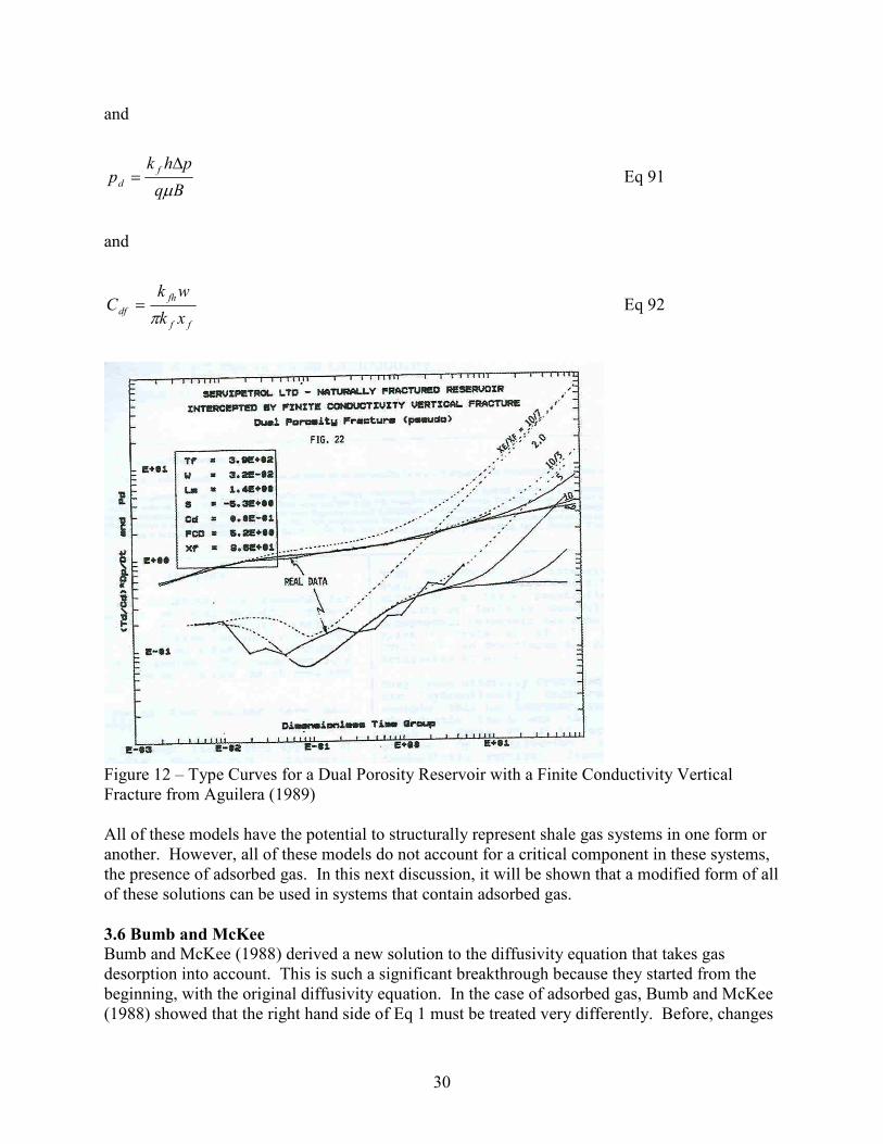
30
and
Bq
phkp
f
d µ
∆=
Eq 91
and
ff
fh
dfxk
wkC
π=
Eq 92
Figure 12 – Type Curves for a Dual Porosity Reservoir with a Finite Conductivity Vertical
Fracture from Aguilera (1989)
All of these models have the potential to structurally represent shale gas systems in one form or
another. However, all of these models do not account for a critical component in these systems,
the presence of adsorbed gas. In this next discussion, it will be shown that a modified form of all
of these solutions can be used in systems that contain adsorbed gas.
3.6 Bumb and McKee
Bumb and McKee (1988) derived a new solution to the diffusivity equation that takes gas
desorption into account. This is such a significant breakthrough because they started from the
beginning, with the original diffusivity equation. In the case of adsorbed gas, Bumb and McKee
(1988) showed that the right hand side of Eq 1 must be treated very differently. Before, changes

31
in system density and porosity were only the result of gas and/or formation expansion. Now,
desorption must be considered. Thus, assuming a Langmuir desorption isotherm the right side of
Eq 1 is expanded to yield (Bumb and McKee, 1988)
( )
∂
∂+
∂∂
+∂∂
=∂∂
t
V
ttt
escρ
φρ
ρφφρ
Eq 93
where
pp
pvV
L
Le +=
Eq 94
and vL is the adsorbed gas per cubic foot of rock and pL is the Langmuir pressure.
The only difference between this equation and the original version of the diffusivity equation
proposed earlier is the third term which accounts for adsorption. Substituting the expanded right
hand side of the above equation, the Langmuir isotherm, and the real gas equation of state into
the diffusivity equation yields
+∂∂
+∂∂
+
∂∂
=
∂∂
∂∂
pp
pv
ttRTz
pM
RTz
pM
tr
p
RTz
pMr
r
k
r L
Lscρ
φφ
µ1
Eq 95
Assuming that molecular gas composition and temperature are constant and rearranging
∂∂
+∂∂
+∂∂
∂∂
+∂∂
∂∂
=
∂∂
∂∂
p
p
pp
pv
tz
p
p
p
tz
p
p
p
z
p
tr
p
z
pr
r
k
r L
Lsc ρφφ
ρφ
φµ
1
Eq 96
Differentiating and recognizing again the definitions of compressibility yields
t
p
pp
pvcc
z
p
r
p
z
pr
r
k
rL
LLsc
fg ∂∂
+++=
∂∂
∂∂
2)(
1
φρρ
φµ
Eq 97
It is important to examine this current form of the diffusivity equation. The gas and formation
compressibility are the same as they are in the original diffusivity equation. The difference is the
third term again. It represents a correction to the total system compressibility to account for the
adsorbed gas (Bumb and McKee, 1988). This compressibility is based on the Langmuir
desorption isotherm. Now, this new total system compressibility is
32
adsfgt cccc ++=*
Eq 98
where
2)( pp
pvc
L
LLsc
ads +=φρρ
Eq 99
3.7 Spivey and Semmelbeck The most recent efforts to accurately analyze production data analytically come from Spivey and
Semmelbeck (1995) and Clarkson et al. (2007). Spivey and Semmelbeck (1995) used a
numerical reservoir simulator to demonstrate the behavior of coalbed methane and shale gas
reservoirs. Their model is simply a high porosity fracture sandwiched between two low
kφ “matrix” layers (i.e. a slab dual porosity model). They compared the simulator’s results to a
dual porosity analytical model and got accurate results when they used the modified version of
the total system compressibility presented by Bumb and McKee (1988). They varied several
parameters including dimensionless radius (rd), interporosity flow coefficient (λ), storativity ratio (ω), flowing bottomhole pressure (pwf), and Langmuir volume (vL).
What is unique about their approach is that the effects of desorption are entirely accounted for by
using the adjusted total compressibility. The Langmuir Volume (vL) and the Langmuir pressure
(pL) are incorporated to account for adsorption. Spivey and Semmelbeck (1995) use standard
equations for qd and td, but substitute in Bumb and McKee’s (1988) definition of compressibility.
f
Lscsc
LLsc
gwwwt cppzT
TzpVpcScSc +
++−+=
2
*
)()1(
φ Eq 100
As expected, the effects of rd and pwf are large and can readily be identified. However, λ, ω, and vL all work together to influence production rate. The Langmuir volume affects how much gas
will actually be available to flow while interporosity flow coefficient and the storativity ratio
affect it’s ability to flow and how it flows. At high vL, the effects of λ and ω are more pronounced, especially at late time. At small values of vL and at early time, it is very difficult to
discern the effects of changing λ and ω. This difficulty could be magnified when using actual production data as opposed to simulated data.
3.8 Summary of Literature Review
There have been significant advances in the field of production data analysis in the last ten years.
Arguably, the methodology behind it is as mathematically grounded as that of pressure transient
analysis. The advent of material balance time, the use of pseudofunctions, and the proliferation
33
of software to implement these things are the largest contributors to this new, more rigorous
approach.
Shale gas reservoirs still present an enormous challenge due to their complexity. Generally
speaking, a shale gas reservoir is probably best represented, analytically, by a dual porosity
model with hydraulic fractures. It is expected that these reservoirs should behave similarly to
their conventional reservoir counterparts. Specifically, all of the various flow regimes that one
would expect should be visible on the derivative plots commonly used in pressure transient
analysis. It has been shown that there is an analytical approach to account for adsorbed gas in
the form of an adjusted compressibility. If this is all that is needed, there should be no reason for
the appearance of the various flow regimes to be altered dramatically. However, the effect (s) of
adsorption on dimensionless type curves is unknown except that it will most likely be very subtle
as was seen when Spivey and Semmelbeck (1995) examined its effect on production data. In
addition, it is not clear how the analysis approach impacts the outcome of an analysis when
adsorption is present.
The Clarkson et al. (2007) work also used the Bumb and McKee (1988) transformation in a
material balance time approach in coalbed methane systems. They also incorporated relative
permeability effects. They showed that these adjustments were necessary and were applied to
radial flow models.
For instance, does analyzing a shale gas reservoir as a single porosity system yield vastly
different results than if one analyzes it as a dual porosity system with hydraulic fractures? If so,
is this error due to the effect of adsorption or just a poor choice of an analytical model? In the
coming chapters, the effects of adsorption on commonly used dimensional and dimensionless
type curves will be shown. In addition, a methodology for analyzing production data from
adsorbed reservoirs using analytical type curves that do not account for adsorption will be
detailed. Finally, the effects applying this methodology to one simulated and two field cases and
the effects of assuming different reservoir systems (single porosity, dual porosity, hydraulically
fractured, and dual porosity with hydraulic fracture) will be shown and explained.

34
4. SIMULATION MODELING
This section shows that it is completely possible to correctly retrieve system parameters if one
knows the system type. The analytic solutions for the various systems (single porosity, dual
porosity, hydraulic fracture, and dual porosity with hydraulic fracture models) were compared to
numerical simulation models. The analytic solutions would be used with real production data to
estimate key reservoir parameters. The effects of all the parameters that influence these analytic
solutions can be seen with clean simulated data. First, systems produced at constant rate and
then constant pressure will be examined. Recall that one of the objectives of this work requires
the analysis of production data as equivalent constant rate data. Adsorption will be discussed in
the next chapter.
To aid in understanding the complexities of all the various systems involved, several finite-
difference flow simulation models were constructed. Variations of these models show that the
effects predicted by the fundamental models of pressure transient analysis (PTA) were visible.
The finite-difference simulator used was GEM from the Computer Modeling Group.
PTA is best done with dimensionless variables. Previous researchers have shown that the use of
dimensionless variables also improves analysis of production data. The main purpose of
discussing pressure transient analysis techniques is to show that the visual indicators of flow
regimes are consistent across all types of analysis. Boundary dominated flow is a unit-slope in
both the pressure and pressure derivative curves in standard PTA; it can be any number of shapes
in standard production data analysis in use today. To review concepts mentioned earlier,
dimensionless time and dimensionless pressure are convenient arrangements of variables that
allow the diffusivity equation to be solved more easily. For the purposes of this work,
dimensionless pressure and dimensionless time will be generally defined by:
g
wfi
wdTq
pmpmkhp
1422
)]()([ −= Eq 101
2)(
00634.0
wtigi
drc
ktt
φµ= Eq 102
4.1 Systems Produced at Constant Terminal Rate
The first simulation model constructed (Model 1) was a single-layer, radial, single porosity
(homogeneous) gas reservoir. There is one well in the center of the model. The model
parameters are listed in Table 1. Note that this model is not representative of shale-gas systems;
a separate model with parameters more realistic for shale gas systems was also constructed and
will be discussed in Chapter 6. This model and its variations can be thought of as the base case.
Original gas in place for Model 1 is 188 BSCF. The grid system has 50 divisions along the
radius arranged logarithmically increasing in size from the center. Model 1 was first run at a
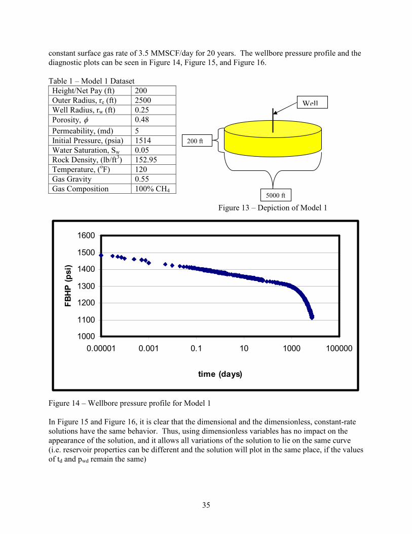
35
constant surface gas rate of 3.5 MMSCF/day for 20 years. The wellbore pressure profile and the
diagnostic plots can be seen in Figure 14, Figure 15, and Figure 16.
Table 1 – Model 1 Dataset
Height/Net Pay (ft) 200
Outer Radius, re (ft) 2500
Well Radius, rw (ft) 0.25
Porosity, φ 0.48
Permeability, (md) 5
Initial Pressure, (psia) 1514
Water Saturation, Sw 0.05
Rock Density, (lb/ft3) 152.95
Temperature, (oF) 120
Gas Gravity 0.55
Gas Composition 100% CH4
Figure 13 – Depiction of Model 1
Figure 14 – Wellbore pressure profile for Model 1
In Figure 15 and Figure 16, it is clear that the dimensional and the dimensionless, constant-rate
solutions have the same behavior. Thus, using dimensionless variables has no impact on the
appearance of the solution, and it allows all variations of the solution to lie on the same curve
(i.e. reservoir properties can be different and the solution will plot in the same place, if the values
of td and pwd remain the same)
1000
1100
1200
1300
1400
1500
1600
0.00001 0.001 0.1 10 1000 100000
time (days)
FBHP (psi)
Well
200 ft
5000 ft

36
Dimensional Type Curve
100000
1000000
10000000
100000000
0.00001 0.0001 0.001 0.01 0.1 1 10 100 1000 10000
time (days)
dm(pwf) or td*d[ln(m(pwf))]/dtd
m(Pwf)'
dm(Pwf)
Radial Flow
Boundary Dominated
Flow: Unit-Slope
Figure 15 – Diagnostic plot for Model 1 using dimensional plotting functions
0.1
1
10
100
0.0000001 0.00001 0.001 0.1 10
td
pd or td*d(lnPd)/dtd
Pd
Pd'
Analy. Soln
Figure 16 – Diagnostic plot for Model 1 using dimensionless plotting functions
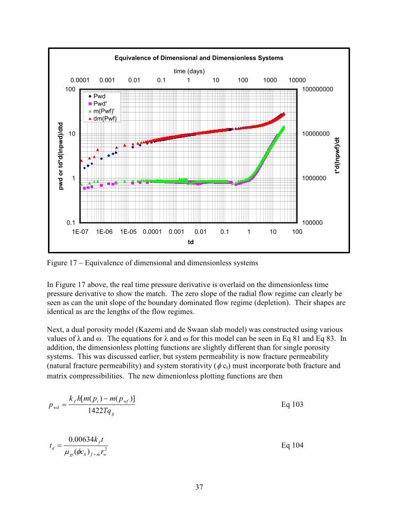
37
Equivalence of Dimensional and Dimensionless Systems
0.1
1
10
100
1E-07 1E-06 1E-05 0.0001 0.001 0.01 0.1 1 10 100
td
pwd or td*d(lnpwd)/dtd
100000
1000000
10000000
100000000
0.0001 0.001 0.01 0.1 1 10 100 1000 10000
time (days)
t*d(lnpwf)/dt
Pwd
Pwd'
m(Pwf)'
dm(Pwf)
Figure 17 – Equivalence of dimensional and dimensionless systems
In Figure 17 above, the real time pressure derivative is overlaid on the dimensionless time
pressure derivative to show the match. The zero slope of the radial flow regime can clearly be
seen as can the unit slope of the boundary dominated flow regime (depletion). Their shapes are
identical as are the lengths of the flow regimes.
Next, a dual porosity model (Kazemi and de Swaan slab model) was constructed using various
values of λ and ω. The equations for λ and ω for this model can be seen in Eq 81 and Eq 83. In
addition, the dimensionless plotting functions are slightly different than for single porosity
systems. This was discussed earlier, but system permeability is now fracture permeability
(natural fracture permeability) and system storativity (φ ct) must incorporate both fracture and matrix compressibilities. The new dimenionless plotting functions are then
g
wfif
wdTq
pmpmhkp
1422
)]()([ −= Eq 103
2)(
00634.0
wmftigi
f
drc
tkt
+
=φµ
Eq 104
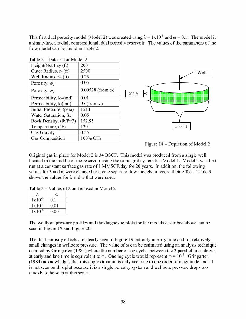
38
This first dual porosity model (Model 2) was created using λ = 1x10⁻⁸ and ω = 0.1. The model is
a single-layer, radial, compositional, dual porosity reservoir. The values of the parameters of the
flow model can be found in Table 2.
Table 2 – Dataset for Model 2
Height/Net Pay (ft) 200
Outer Radius, re (ft) 2500
Well Radius, rw (ft) 0.25
Porosity, mφ 0.05
Porosity, fφ 0.00528 (from ω)
Permeability, km(md) 0.01
Permeability, kf(md) 95 (from λ)
Initial Pressure, (psia) 1514
Water Saturation, Sw 0.05
Rock Density, (lb/ft^3) 152.95
Temperature, (oF) 120
Gas Gravity 0.55
Gas Composition 100% CH4
Figure 18 – Depiction of Model 2
Original gas in place for Model 2 is 34 BSCF. This model was produced from a single well
located in the middle of the reservoir using the same grid system has Model 1. Model 2 was first
run at a constant surface gas rate of 1 MMSCF/day for 20 years. In addition, the following
values for λ and ω were changed to create separate flow models to record their effect. Table 3
shows the values for λ and ω that were used.
Table 3 – Values of λ and ω used in Model 2
λ ω
1x10⁻⁸ 0.1
1x10⁻⁷ 0.01
1x10⁻⁶ 0.001
The wellbore pressure profiles and the diagnostic plots for the models described above can be
seen in Figure 19 and Figure 20.
The dual porosity effects are clearly seen in Figure 19 but only in early time and for relatively
small changes in wellbore pressure. The value of ω can be estimated using an analysis technique
detailed by Gringarten (1984) where the number of log cycles between the 2 parallel lines drawn
at early and late time is equivalent to ω. One log cycle would represent ω = 10-1. Gringarten
(1984) acknowledges that this approximation is only accurate to one order of magnitude. ω = 1
is not seen on this plot because it is a single porosity system and wellbore pressure drops too
quickly to be seen at this scale.
Well
200 ft
5000 ft

39
Effects of Omega
1490
1491
1492
1493
1494
1495
1496
1497
1498
0.000001 0.0001 0.01 1 100 10000
time (days)
FBHP (psi)
Omega = 0.01
Omega = 0.1
Omega = 0.1
Figure 19 – Wellbore pressure profiles for Model 2 showing the effect of omega

40
Effects of Omega
0.001
0.01
0.1
1
10
100
0.01 0.1 1 10 100 1000 10000 100000 100000
0
1E+07 1E+08
td
td*ln(Pd)/dtd
Omg = 0.1Omg = 0.01Omg = 0.001Analy. Soln.
Effects of Omega
Radial Flow
Figure 20 – Diagnostic plot of Model 2 showing the effects of lambda
Figure 20 shows the derivative plot for a dual porosity system. Note that all the systems merge
together during late-time, radial flow. This is expected since all the models are the same
physical size and are produced at the same constant rate. Boundary dominated flow was not
reached here because the models were not allowed to run for a long enough period of time. The
analytical solution shown here used input values from the simulator data file. It shows the
“right” answer for ω = 0.01. The other curves shown in Figure 20 are variations to the simulated
data file to show the effects of ω.
Figure 21 and Figure 22 show the effects of changing the value of λ. It should be noted that
these plots actually have some effects of ω as well (since the model has ω = 0.4 which is the
result of setting fracture porosity equal to formation porosity). ω is not 0.5 because matrix
compressibility and fracture compressibility are not equal in this model. This also explains the
very small “hump” that is characteristic of dual porosity systems. This “hump” is very small for
large values of ω. The λ term only serves to shift the position of the trough created by the effects
of ω. The radial flow regime is still present as a horizontal line on the derivative plot. However,
late time radial flow may not be achieved since the effects of λ can last until the beginning of
boundary dominated flow. This can be seen in both the cases of λ = 1x10⁻⁸ and of λ = 1x10
-7.
The dual porosity analytic model is a much better representation of shale gas reservoirs than a
single porosity system. However, it does not address the presence of hydraulic fractures that are
common to shale gas reservoirs. The next series of plots will apply to the common scenario of

41
Effects of Lambda
1300
1350
1400
1450
1500
1550
0.00001 0.0001 0.001 0.01 0.1 1 10 100 1000 10000
Time (days)
FBHP (psi)
Lambda = 1E-8
Lambda = 1E-7
Lambda = 1E-6
Figure 21 – Wellbore pressure profiles for Model 2 showing the effects of lambda
Effects of Lambda
0.1
1
10
1 100 10000 1000000 100000000 10000000000 1E+12
td
td*dln(pd)/dtd
Lam = 1E-6
Lam = 1E-7
Lam = 1E-8
Analytical Model
Figure 22 – Diagnostic plot for Model 2 showing the effects of lambda

42
hydraulically fractured reservoirs. The development of the plotting functions for these systems
was discussed earlier. For review, the dimensionless time and pressure variables are presented
below.
wxc
tk
C
t
ftmm
m
df
d
µφπ
00634.0=
Eq 105
g
m
wdTq
pmhkp
1422
)(∆=
Eq 106
where
)()()( wfi pmpmpm −=∆ Eq 107
A hydraulic fracture model (Model 3) was constructed in a different manner than the previous
models. As a model, hydraulic fractures are very thin, vertical structures that generally penetrate
the entire thickness of a reservoir and extend for several hundred feet horizontally. The width of
the fracture itself is rarely more than a fraction of an inch.
In a finite difference simulator, this kind of structure is difficult to create. There is really only
one way to achieve the desired result, local grid refinement. For this model, each of the grid
cells around the well were subdivided into multiple cells. The refinement was increased closer to
the well and the fracture. This resulted in the grid cells that represent the fracture being 4 inches
in width. This allowed the permeability to be modified for only a very narrow streak of the
model on either side of the well and was the smallest grid size allowed in the model.
Figure 23 shows map views of Model 3. It shows the local grid refinement as it appears on a
large scale and on a close up view of the area around the well. The fracture is visible as a thin
red line.
The wellbore pressure profiles and type curves for this model and models with different values
of Cdf (Eq 88) are presented in Figure 25 and Figure 26.
The effects of the hydraulic fracture are imbedded in the Cdf term. These effects are visible in
derivative plot in Figure 26 at only early time. They consist of a ¼ slope that is visible for a
short length of time depending on the value of Cdf. The larger values of Cdf (which happen to
coincide with large values of fracture permeability) extend the effects into slightly later time.
However, all of the models merge together at late-time to form the zero-slope pseudo-radial flow
and then the unit-slope boundary-dominated flow.

43
Figure 23 – Aerial views of Model 3
Table 4 – Dataset for Model 3
Height/Net Pay (ft) 40
Outer Radius, re (ft) 2604
Well Radius, rw (ft) 0.25
Porosity, mφ 0.10
xf (ft) 200(Cdf = 0.03)
Permeability, km(md) 0.5
Permeability, kfh(md) 25 (Cdf = 0.03)
Initial Pressure, (psia) 1514
Water Saturation, Sw 0.05
Rock Density, (lb/ft^3) 152.95
Temperature, (oF) 225
Gas Gravity 0.6
Gas Composition 100% CH4
Figure 24 – Depiction of Model 3
Well
Fracture
Well Fracture
40 ft
5280 ft
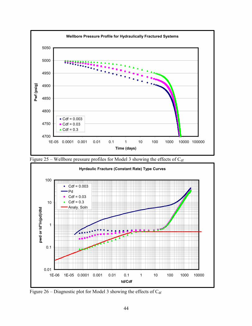
44
Wellbore Pressure Profile for Hydraulically Fractured Systems
4700
4750
4800
4850
4900
4950
5000
5050
1E-05 0.0001 0.001 0.01 0.1 1 10 100 1000 10000 100000
Time (days)
Pwf (psig)
Cdf = 0.003
Cdf = 0.03
Cdf = 0.3
Figure 25 – Wellbore pressure profiles for Model 3 showing the effects of Cdf
Hyrdaulic Fracture (Constant Rate) Type Curves
0.01
0.1
1
10
100
1E-06 1E-05 0.0001 0.001 0.01 0.1 1 10 100 1000 10000
td/Cdf
pwd or td*ln(pd)/dtd
Cdf = 0.003
Pd
Cdf = 0.03
Cdf = 0.3
Analy. Soln
Figure 26 – Diagnostic plot for Model 3 showing the effects of Cdf

45
The next complication added to the system is to assume dual porosity systems with hydraulic
fractures that are produced at constant rate. The plotting functions were discussed earlier and are
essentially a combination of those used for hydraulically fractured systems and those used for
dual porosity systems. They are
wxc
tk
C
t
ft
f
df
d
φµ
π00634.0=
Eq 108
g
f
wdTq
pmhkp
1422
)(∆=
Eq 109
Model 4 was constructed similarly to Model 3. The exact same grid refinement was used to
create the very thin gridblocks necessary for the hydraulic fracture. The only difference is that
Model 4 is a dual porosity model was used, so an additional permeability, kf (natural fracture
permeability), was defined. A schematic of the model is shown in Figure 27 and a list of its
properties can be seen in
Table 5.
Table 5 – Dataset for Model 4
Height/Net Pay (ft) 40
Outer Radius, re (ft) 2604
Well Radius, rw (ft) 0.25
Porosity, mφ 0.10
Porosity, fφ 0.001 (ω = 0.01)
xf (ft) 200
Permeability, km (md) 0.5
Permeability, kf (md) 94 (λ = 1E-5)
Permeability, kfh (md) 250
Initial Pressure, (psia) 1514
Water Saturation, Sw 0.05
Rock Density, (lb/ft^3) 152.95
Temperature, (oF) 225
Gas Gravity 0.6
Gas Composition 100% CH4
Figure 27 – Depiction of Model 4
The effect of different ratios of xe/xf (reservoir half-length to fracture half-length) is shown in
Figure 28 and a noticeable vertical shift is seen. The effects of ω and λ are still visible, although
it is admittedly hard to see those of ω. This is due to the very rapid drawdown that occurs due to
the presence of the hydraulic fracture.
Well Fracture
40 ft
5280 ft

46
Wellbore Pressure Profile for Dual Porosity Systems
w/Hydraulic Fracture (Effects of xe/xf)
4998.5
4998.7
4998.9
4999.1
4999.3
4999.5
4999.7
4999.9
5000.1
5000.3
5000.5
0.000001 0.0001 0.01 1 100 10000 1000000
Time (days)
FBHP (psig)
Lambda 1E-5, Xe/Xf = 13
Lambda 1E-5, Xe/Xf = 5.5
Lambda 1E-6, Xe/Xf = 13
Lambda 1E-6, Xe/Xf = 5.5
Figure 28 – Wellbore pressure profile for Model 4 showing the effects of fracture half-length
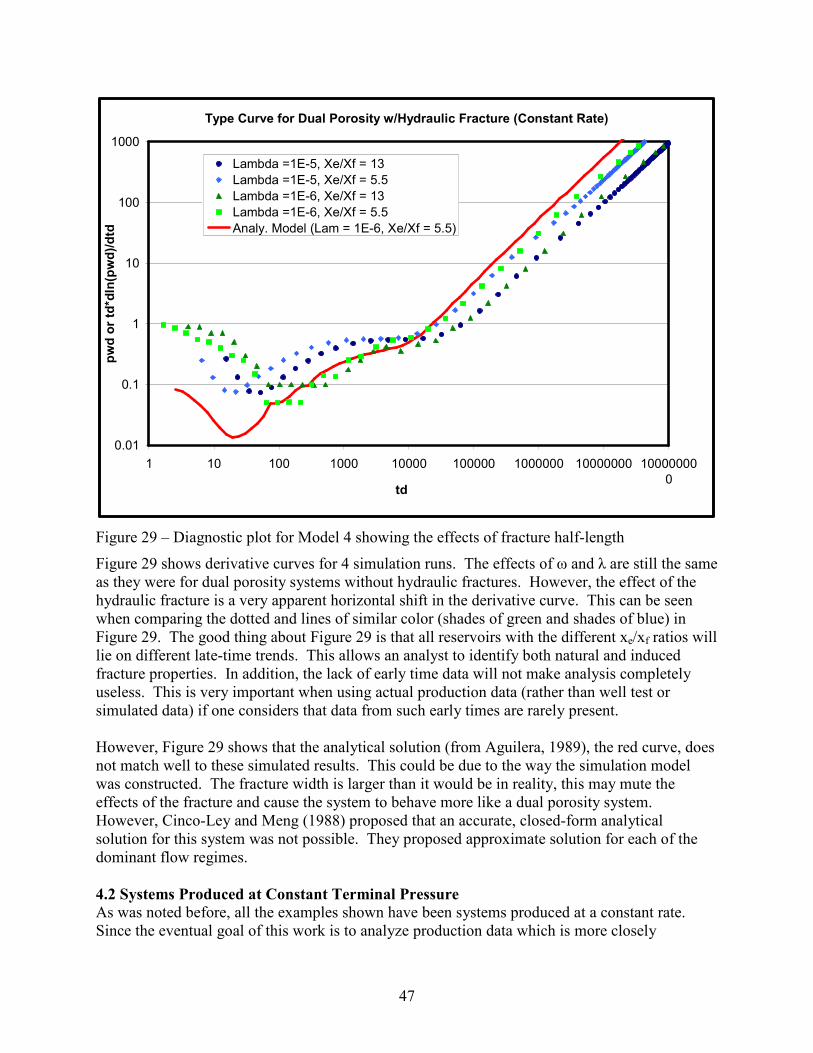
47
Type Curve for Dual Porosity w/Hydraulic Fracture (Constant Rate)
0.01
0.1
1
10
100
1000
1 10 100 1000 10000 100000 1000000 10000000 10000000
0td
pwd or td*dln(pwd)/dtd
Lambda =1E-5, Xe/Xf = 13
Lambda =1E-5, Xe/Xf = 5.5
Lambda =1E-6, Xe/Xf = 13
Lambda =1E-6, Xe/Xf = 5.5
Analy. Model (Lam = 1E-6, Xe/Xf = 5.5)
Figure 29 – Diagnostic plot for Model 4 showing the effects of fracture half-length
Figure 29 shows derivative curves for 4 simulation runs. The effects of ω and λ are still the same
as they were for dual porosity systems without hydraulic fractures. However, the effect of the
hydraulic fracture is a very apparent horizontal shift in the derivative curve. This can be seen
when comparing the dotted and lines of similar color (shades of green and shades of blue) in
Figure 29. The good thing about Figure 29 is that all reservoirs with the different xe/xf ratios will
lie on different late-time trends. This allows an analyst to identify both natural and induced
fracture properties. In addition, the lack of early time data will not make analysis completely
useless. This is very important when using actual production data (rather than well test or
simulated data) if one considers that data from such early times are rarely present.
However, Figure 29 shows that the analytical solution (from Aguilera, 1989), the red curve, does
not match well to these simulated results. This could be due to the way the simulation model
was constructed. The fracture width is larger than it would be in reality, this may mute the
effects of the fracture and cause the system to behave more like a dual porosity system.
However, Cinco-Ley and Meng (1988) proposed that an accurate, closed-form analytical
solution for this system was not possible. They proposed approximate solution for each of the
dominant flow regimes.
4.2 Systems Produced at Constant Terminal Pressure
As was noted before, all the examples shown have been systems produced at a constant rate.
Since the eventual goal of this work is to analyze production data which is more closely
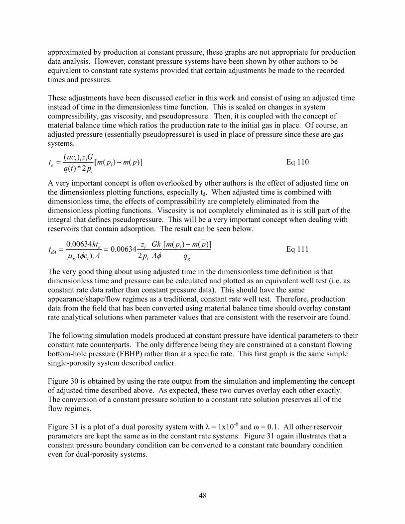
48
approximated by production at constant pressure, these graphs are not appropriate for production
data analysis. However, constant pressure systems have been shown by other authors to be
equivalent to constant rate systems provided that certain adjustments be made to the recorded
times and pressures.
These adjustments have been discussed earlier in this work and consist of using an adjusted time
instead of time in the dimensionless time function. This is scaled on changes in system
compressibility, gas viscosity, and pseudopressure. Then, it is coupled with the concept of
material balance time which ratios the production rate to the initial gas in place. Of course, an
adjusted pressure (essentially pseudopressure) is used in place of pressure since these are gas
systems.
)]()([2*)(
)(pmpm
ptq
Gzct i
i
iita −=
µ Eq 110
A very important concept is often overlooked by other authors is the effect of adjusted time on
the dimensionless plotting functions, especially td. When adjusted time is combined with
dimensionless time, the effects of compressibility are completely eliminated from the
dimensionless plotting functions. Viscosity is not completely eliminated as it is still part of the
integral that defines pseudopressure. This will be a very important concept when dealing with
reservoirs that contain adsorption. The result can be seen below.
g
i
i
i
itgi
adA
q
pmpm
A
Gk
p
z
Ac
ktt
)]()([
200634.0
)(
00634.0 −==
φφµ Eq 111
The very good thing about using adjusted time in the dimensionless time definition is that
dimensionless time and pressure can be calculated and plotted as an equivalent well test (i.e. as
constant rate data rather than constant pressure data). This should have the same
appearance/shape/flow regimes as a traditional, constant rate well test. Therefore, production
data from the field that has been converted using material balance time should overlay constant
rate analytical solutions when parameter values that are consistent with the reservoir are found.
The following simulation models produced at constant pressure have identical parameters to their
constant rate counterparts. The only difference being they are constrained at a constant flowing
bottom-hole pressure (FBHP) rather than at a specific rate. This first graph is the same simple
single-porosity system described earlier.
Figure 30 is obtained by using the rate output from the simulation and implementing the concept
of adjusted time described above. As expected, these two curves overlay each other exactly.
The conversion of a constant pressure solution to a constant rate solution preserves all of the
flow regimes.
Figure 31 is a plot of a dual porosity system with λ = 1x10⁻⁶ and ω = 0.1. All other reservoir
parameters are kept the same as in the constant rate systems. Figure 31 again illustrates that a
constant pressure boundary condition can be converted to a constant rate boundary condition
even for dual-porosity systems.

49
Equivalence of Constant Pressure
0.1
1
10
100
0.1 1 10 100 1000 10000 100000 100000
0
1E+07 1E+08 1E+09
td
pd or t*d(lnPd)/dt
Const Rate Pd (rate)
Pd (Press) Const Pressure
Figure 30 – Diagnostic plot showing the equivalence of constant rate and constant pressure
derivative curves
Figure 32, Figure 33, and Figure 34 isolate the effects of the dual porosity parameters λ and ω in
constant pressure systems. The rate-decline type curves are the dimensional equivalent of
wellbore pressure profiles for constant rate systems. The x-axis is the log(t) and the y-axis is
normalized rate. Plotting the data in this way (Figure 32 and Figure 33) yields plots that look
very similar to Fetkovich’s decline curves for liquid systems. Note that the plotting functions are
quite different though. The equation for normalized rate is
)()( wfi
g
normpmpm
−= . Eq 112
Figure 32 and Figure 33 show the effects of lambda and omega on dimensional type curves for
constant pressure systems. Note the difference in character of the dimensional plots in Figure 32
and Figure 33 and the dimensionless plot in Figure 34. In the opinion of this author, having a
unified late-time curve for a given dimensionless radius makes Figure 34 much easier to read.
Admittedly, a similar effect can be achieved using a Fetkovich style plot.
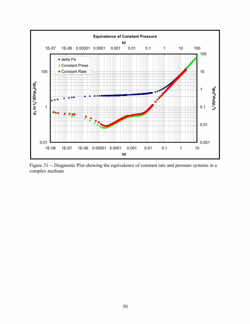
50
Equivalence of Constant Pressure
0.01
1
100
1E-08 1E-07 1E-06 0.00001 0.0001 0.001 0.01 0.1 1 10
td
pd or t d*d(lnpd)/dt d
0.001
0.01
0.1
1
10
100
1E-07 1E-06 0.00001 0.0001 0.001 0.01 0.1 1 10 100
td
t d*d(lnpd)/dt d
delta Pd
Constant Press
Constant Rate
Figure 31 -- Diagnostic Plot showing the equivalence of constant rate and pressure systems in a
complex medium

51
Rate-Decline Type Curves for Dual Porosity Systems
(Effects of Omega)
0.0001
0.001
0.01
0.00001 0.0001 0.001 0.01 0.1 1 10 100 1000
Time (days)
Qg/(Ppi - Ppwf)
Omg = 0.1
Omg = 0.01
Omg = 0.001
Figure 32 -- Rate-decline plot showing the effects of omega

52
Rate-Decline Type Curves for Dual Porosity Systems
(Effects of Lambda)
0.0000001
0.000001
0.00001
0.0001
0.001
0.01
0.0001 0.001 0.01 0.1 1 10 100 1000 10000
Time (days)
Qg/(Ppi - Ppavg)
Lambda = 1E-8
Lambda = 1E-7
Figure 33 – Rate-Decline plot showing the effects of lambda
53
Constant Pressure Type Curves for Dual Porosity Systems
(Shown here converted to Constant Rate)
0.001
0.01
0.1
1
10
100
0.0000001 0.000001 0.00001 0.0001 0.001 0.01 0.1 1 10
tda
t da*ln(p
wd)/dt da
Lambda 1E-8, Omg 0.1
Lambda 1E-8, Omg 0.01
Lambda 1E-8, Omg 0.001
Lambda 1E-7, Omg 0.1
Lambda 1E-7, Omg 0.01
Lambda 1E-7, Omg 0.001
Figure 34 – Derivative type curve for constant pressure systems. Shown here converted to an
equivalent constant rate system
The effects of λ and ω in constant-pressure systems after the systems are converted to constant-
rate are shown in Figure 34, and are essentially the same as they are in constant-rate systems.
This is to be expected since the technique of material balance time was used.
Figure 35 and Figure 36 are simulated data for single porosity hydraulically fractured systems
produced at constant pressure. The models used to create these datasets are identical to those
used for constant rate, hydraulically fractured systems with the exception of the boundary
condition used at the well. The technique of material balance time was used to convert the
constant pressure data to constant rate data, so it could be displayed on pressure-transient style
plots. The equation for tda is slightly different for hydraulically fractured systems than for the
systems discussed previously. Recall that the x-axis plotting function for this type of system is
td/Cdf. This means that there will be additional terms in the equation for tda.
g
imf
i
i
fh
fm
itgi
afh
dAq
pmpm
A
Gk
w
x
p
z
wk
xk
Ac
tkt
)]()([01002.0
)(
00634.0 −==
φ
π
φµ Eq 113
where
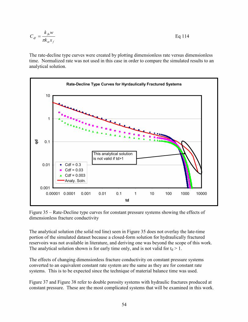
54
fm
fh
dfxk
wkC
π=
Eq 114
The rate-decline type curves were created by plotting dimensionless rate versus dimensionless
time. Normalized rate was not used in this case in order to compare the simulated results to an
analytical solution.
Rate-Decline Type Curves for Hyrdaulically Fractured Systems
0.001
0.01
0.1
1
10
0.00001 0.0001 0.001 0.01 0.1 1 10 100 1000 10000
td
qd
Cdf = 0.3
Cdf = 0.03
Cdf = 0.003
Analy. Soln.
This analytical solution
is not valid if td>1
Figure 35 – Rate-Decline type curves for constant pressure systems showing the effects of
dimensionless fracture conductivity
The analytical solution (the solid red line) seen in Figure 35 does not overlay the late-time
portion of the simulated dataset because a closed-form solution for hydraulically fractured
reservoirs was not available in literature, and deriving one was beyond the scope of this work.
The analytical solution shown is for early time only, and is not valid for td > 1.
The effects of changing dimensionless fracture conductivity on constant pressure systems
converted to an equivalent constant rate system are the same as they are for constant rate
systems. This is to be expected since the technique of material balance time was used.
Figure 37 and Figure 38 refer to double porosity systems with hydraulic fractures produced at
constant pressure. These are the most complicated systems that will be examined in this work.
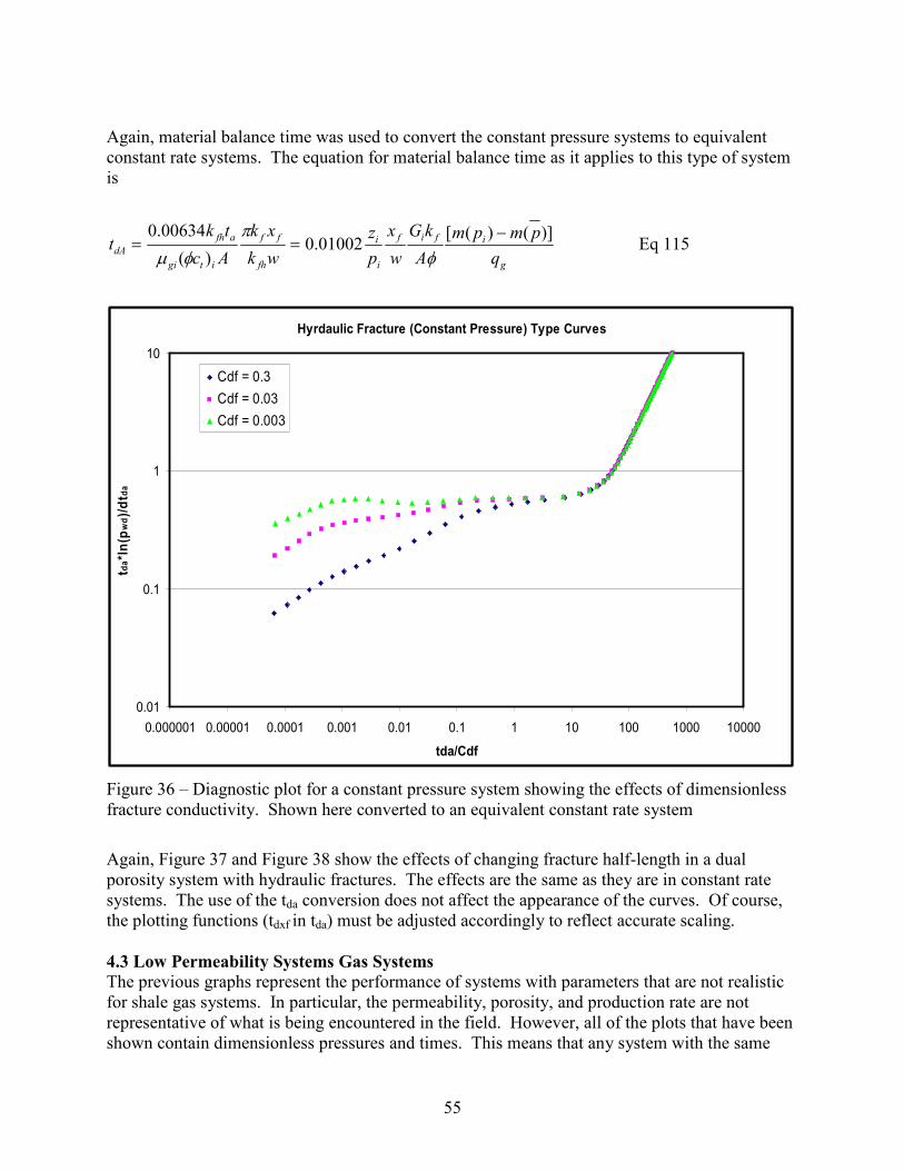
55
Again, material balance time was used to convert the constant pressure systems to equivalent
constant rate systems. The equation for material balance time as it applies to this type of system
is
g
ifif
i
i
fh
ff
itgi
afh
dAq
pmpm
A
kG
w
x
p
z
wk
xk
Ac
tkt
)]()([01002.0
)(
00634.0 −==
φ
π
φµ Eq 115
Hyrdaulic Fracture (Constant Pressure) Type Curves
0.01
0.1
1
10
0.000001 0.00001 0.0001 0.001 0.01 0.1 1 10 100 1000 10000
tda/Cdf
tda*ln(p
wd)/dtda
Cdf = 0.3
Cdf = 0.03
Cdf = 0.003
Figure 36 – Diagnostic plot for a constant pressure system showing the effects of dimensionless
fracture conductivity. Shown here converted to an equivalent constant rate system
Again, Figure 37 and Figure 38 show the effects of changing fracture half-length in a dual
porosity system with hydraulic fractures. The effects are the same as they are in constant rate
systems. The use of the tda conversion does not affect the appearance of the curves. Of course,
the plotting functions (tdxf in tda) must be adjusted accordingly to reflect accurate scaling.
4.3 Low Permeability Systems Gas Systems
The previous graphs represent the performance of systems with parameters that are not realistic
for shale gas systems. In particular, the permeability, porosity, and production rate are not
representative of what is being encountered in the field. However, all of the plots that have been
shown contain dimensionless pressures and times. This means that any system with the same

56
Rate-Decline Type Curves for Dual Porosity
Hyrdaulically Fractured Systems
0.000001
0.00001
0.0001
0.001
0.01
0.000001 0.0001 0.01 1 100 10000 1000000
Time (days)
qg/[m(pi) - m(pwf)]
Lam = 1E-5, Xe/Xf = 5.5
Lam = 1E-5, Xe/Xf = 13
Figure 37 – Rate-Decline type curve showing the effects of changing fracture half-length in a
dual porosity system with a hydraulic fracture.
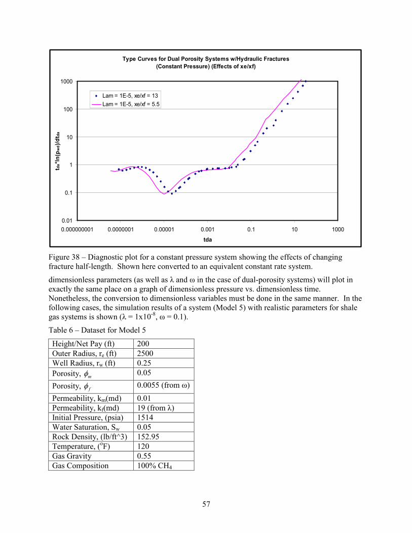
57
Type Curves for Dual Porosity Systems w/Hydraulic Fractures
(Constant Pressure) (Effects of xe/xf)
0.01
0.1
1
10
100
1000
0.000000001 0.0000001 0.00001 0.001 0.1 10 1000
tda
t da*ln(p
wd)/dt da
Lam = 1E-5, xe/xf = 13
Lam = 1E-5, xe/xf = 5.5
Figure 38 – Diagnostic plot for a constant pressure system showing the effects of changing
fracture half-length. Shown here converted to an equivalent constant rate system.
dimensionless parameters (as well as λ and ω in the case of dual-porosity systems) will plot in
exactly the same place on a graph of dimensionless pressure vs. dimensionless time.
Nonetheless, the conversion to dimensionless variables must be done in the same manner. In the
following cases, the simulation results of a system (Model 5) with realistic parameters for shale
gas systems is shown (λ = 1x10⁻⁸, ω = 0.1).
Table 6 – Dataset for Model 5
Height/Net Pay (ft) 200
Outer Radius, re (ft) 2500
Well Radius, rw (ft) 0.25
Porosity, mφ 0.05
Porosity, fφ 0.0055 (from ω)
Permeability, km(md) 0.01
Permeability, kf(md) 19 (from λ)
Initial Pressure, (psia) 1514
Water Saturation, Sw 0.05
Rock Density, (lb/ft^3) 152.95
Temperature, (oF) 120
Gas Gravity 0.55
Gas Composition 100% CH4
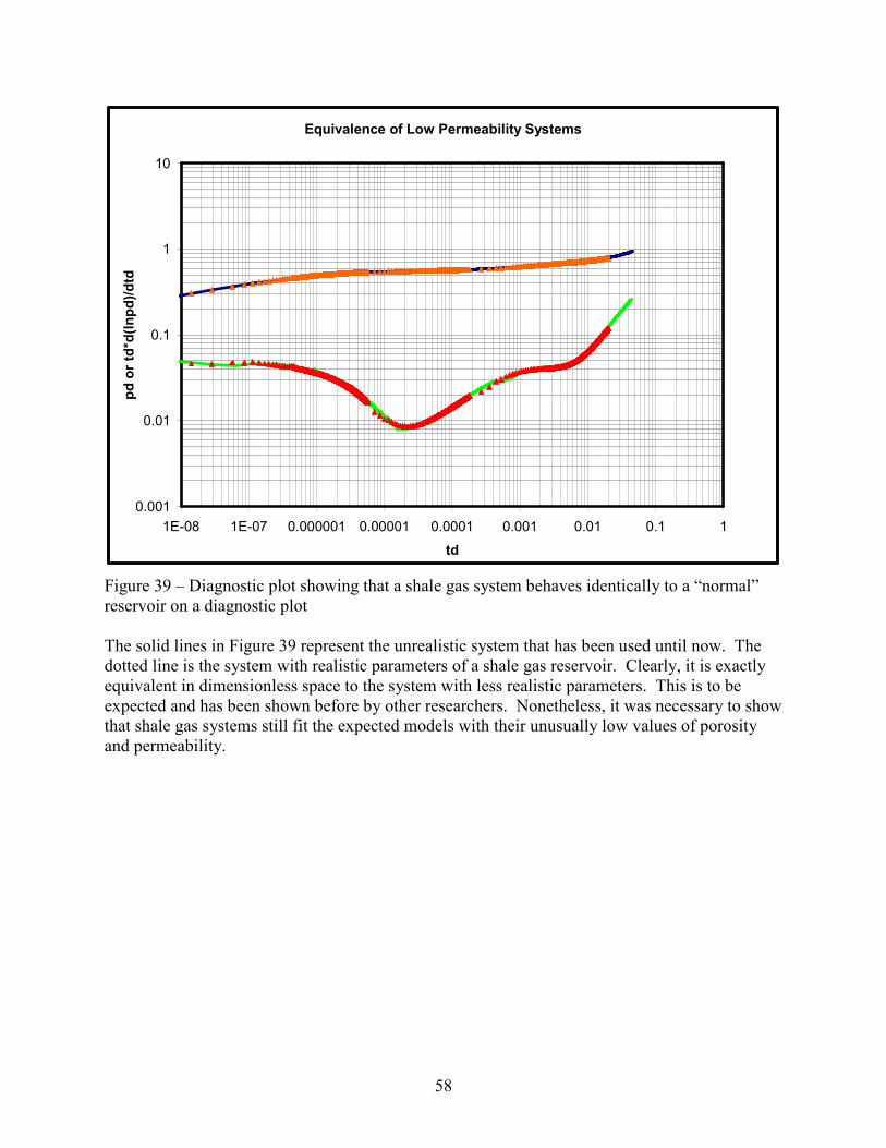
58
Equivalence of Low Permeability Systems
0.001
0.01
0.1
1
10
1E-08 1E-07 0.000001 0.00001 0.0001 0.001 0.01 0.1 1
td
pd or td*d(lnpd)/dtd
Figure 39 – Diagnostic plot showing that a shale gas system behaves identically to a “normal”
reservoir on a diagnostic plot
The solid lines in Figure 39 represent the unrealistic system that has been used until now. The
dotted line is the system with realistic parameters of a shale gas reservoir. Clearly, it is exactly
equivalent in dimensionless space to the system with less realistic parameters. This is to be
expected and has been shown before by other researchers. Nonetheless, it was necessary to show
that shale gas systems still fit the expected models with their unusually low values of porosity
and permeability.

59
5. SIMULATION MODELING OF ADSORPTION
The goal for this section is to show the effect of adsorbed gas on the type curves used for
constant rate and constant pressure production. It will be shown that systems with adsorbed gas
cannot be matched correctly to current analytical solutions if nothing is done to account for the
adsorbed gas. However, if certain steps are taken, adsorption systems can be matched to the
solutions for non-adsorbed systems.
5.1 Adsorption Systems Produced at Constant Terminal Rate
All previous systems that have been mentioned do not contain any adsorbed gas. Since all of the
real shale gas systems have adsorbed gas (Montgomery, et al., 2005), it is necessary to add this
component to the simulation models. The simulator requires that the adsorption data be entered
has an isotherm. It then interpolates, as necessary, between the data points to calculate the
amount of adsorbed gas at any time. Typically, adsorbed values are obtained from lab work in
the form of Langmuir Pressure (pL) and Langmuir Volume (vL). An isotherm can be constructed
using the Langmuir equation:
pp
pvftscfv
L
Lads +
=)/( 3 Eq 116
Adsorption data for all of the models in this chapter is not representative of real shale gas
systems. The values in this chapter were selected to ensure that the effects of adsorption were
highlighted. For the purposes of these next cases, the adsorbed values used were
Table 7 – Langmuir properties
Langmuir
Pressure (psia) 214
Langmuir
Volume (SCF/ft3)
61.2
Rock Density
(g/cm3)
2.45
These properties were chosen to try to investigate effects of adsorption and are not representative
of shale gas systems encountered in the field. Figure 41 and Figure 42 compare a dual-porosity
system (λ = 1x10⁻⁷, ω = 0.01) to a dual porosity system with the same matrix and fracture
properties but also with adsorbed gas. The two models were given identical physical and
reservoir properties except for adsorption being specified for one system. These simulation
models were constructed to be almost identical to the dual porosity models presented earlier,
except that some contain adsorbed gas.
The effects of adsorption are clear in Figure 42. There is a horizontal shift on the derivative
curve. There also is a smaller apparent ω (greater dip at td ≈ 0.003) caused by the method in
which ω is used to calculate the matrix and fracture porosities for the two systems. Recall that ω
is

60
Figure 40 – Langmuir isotherm used in simulation models
Wellbore Pressure Profile for Dual Porosity Systems (Constant Rate)
(Effects of Adsorption)
1465
1470
1475
1480
1485
1490
1495
0.00001 0.0001 0.001 0.01 0.1 1 10 100 1000 10000
time (days)
pwf (psig)
no adsorption
adsorption
Figure 41 – Wellbore pressure profiles for dual porosity systems showing the effects of
adsorption
Adsorption Isotherm
0
10
20
30
40
50
60
0 200 400 600 800 1000 1200
Pressure (psia)
Adsorbed Gas (SCF/ft^3)
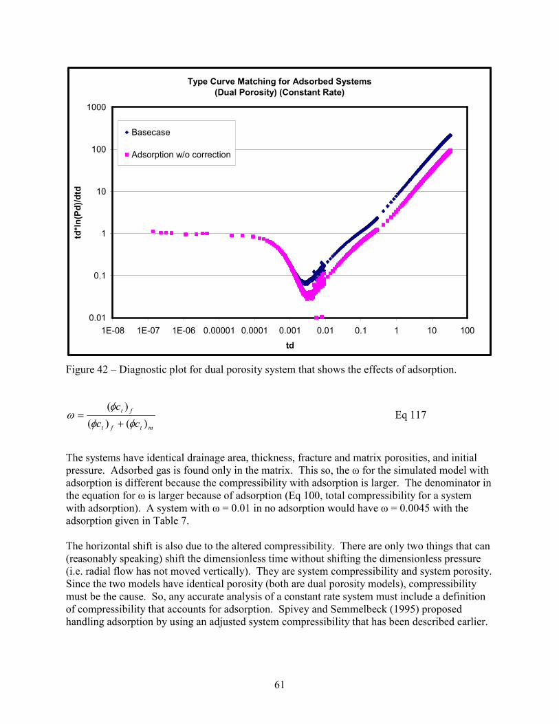
61
Type Curve Matching for Adsorbed Systems
(Dual Porosity) (Constant Rate)
0.01
0.1
1
10
100
1000
1E-08 1E-07 1E-06 0.00001 0.0001 0.001 0.01 0.1 1 10 100
td
td*ln(Pd)/dtd
Basecase
Adsorption w/o correction
Figure 42 – Diagnostic plot for dual porosity system that shows the effects of adsorption.
mtft
ft
cc
c
)()(
)(
φφ
φω
+= Eq 117
The systems have identical drainage area, thickness, fracture and matrix porosities, and initial
pressure. Adsorbed gas is found only in the matrix. This so, the ω for the simulated model with
adsorption is different because the compressibility with adsorption is larger. The denominator in
the equation for ω is larger because of adsorption (Eq 100, total compressibility for a system
with adsorption). A system with ω = 0.01 in no adsorption would have ω = 0.0045 with the
adsorption given in Table 7.
The horizontal shift is also due to the altered compressibility. There are only two things that can
(reasonably speaking) shift the dimensionless time without shifting the dimensionless pressure
(i.e. radial flow has not moved vertically). They are system compressibility and system porosity.
Since the two models have identical porosity (both are dual porosity models), compressibility
must be the cause. So, any accurate analysis of a constant rate system must include a definition
of compressibility that accounts for adsorption. Spivey and Semmelbeck (1995) proposed
handling adsorption by using an adjusted system compressibility that has been described earlier.
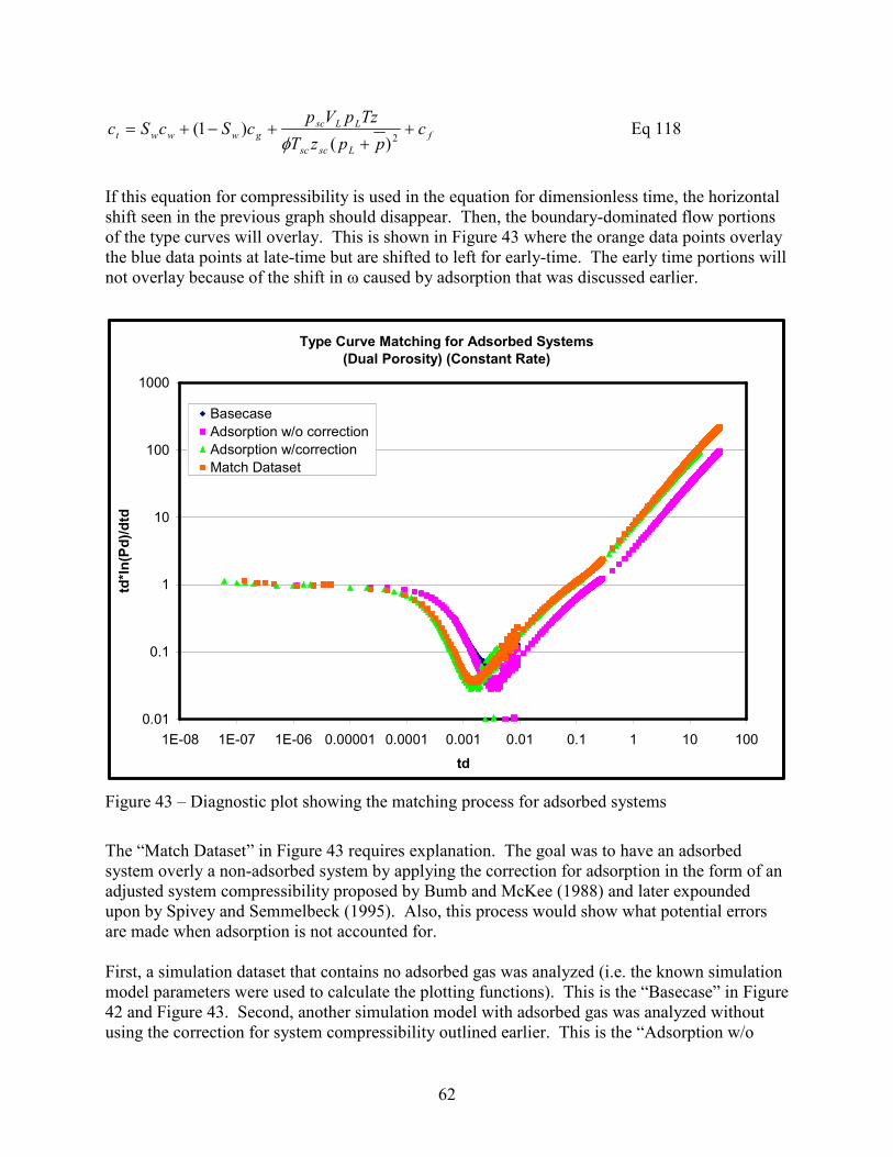
62
f
Lscsc
LLsc
gwwwt cppzT
TzpVpcScSc +
++−+=
2)()1(
φ Eq 118
If this equation for compressibility is used in the equation for dimensionless time, the horizontal
shift seen in the previous graph should disappear. Then, the boundary-dominated flow portions
of the type curves will overlay. This is shown in Figure 43 where the orange data points overlay
the blue data points at late-time but are shifted to left for early-time. The early time portions will
not overlay because of the shift in ω caused by adsorption that was discussed earlier.
Type Curve Matching for Adsorbed Systems
(Dual Porosity) (Constant Rate)
0.01
0.1
1
10
100
1000
1E-08 1E-07 1E-06 0.00001 0.0001 0.001 0.01 0.1 1 10 100
td
td*ln(Pd)/dtd
Basecase
Adsorption w/o correction
Adsorption w/correction
Match Dataset
Figure 43 – Diagnostic plot showing the matching process for adsorbed systems
The “Match Dataset” in Figure 43 requires explanation. The goal was to have an adsorbed
system overly a non-adsorbed system by applying the correction for adsorption in the form of an
adjusted system compressibility proposed by Bumb and McKee (1988) and later expounded
upon by Spivey and Semmelbeck (1995). Also, this process would show what potential errors
are made when adsorption is not accounted for.
First, a simulation dataset that contains no adsorbed gas was analyzed (i.e. the known simulation
model parameters were used to calculate the plotting functions). This is the “Basecase” in Figure
42 and Figure 43. Second, another simulation model with adsorbed gas was analyzed without
using the correction for system compressibility outlined earlier. This is the “Adsorption w/o

63
correction” in Figure 42 and Figure 43. There is a horizontal shift to the right in this dataset
caused by adsorption. Third, the same dataset used in making the “Adsorption w/o correction”
was analyzed using the method described previously to account for adsorption. This causes the
dataset to shift back to the left and overlay the “Basecase” at late-time. This is the “Adsorption
w/correction” in Figure 43. Lastly, a new simulation model (“Match Dataset”) was constructed
to overlay the adsorbed dataset. The “Match Dataset” represents a non-adsorbed system with the
same effective ω as the adsorbed system. Any match of the production data would yield
reservoir parameters that coincide with this analytical solution. The only parameter changed to
attain this match was ω (made smaller). Since the larger compressibility results in a smaller
effective ω, it was necessary to build a non-adsorbed simulation model to match all portions
(early and late time) of the adsorption system.
Note that neither the “Adsorption w/o correction” dataset nor the “Adsorption w/correction”
dataset overlay the “Basecase” at both early and late-time. The “Adsorption w/o correction”
dataset overlays the “Basecase” at early-time despite the presence of adsorbed gas because the pL
used in this model is relatively small. Therefore, adsorption is only a late-time effect. The
“Adsorption w/correction” in Figure 43 is an adsorbed system that has been corrected for
adsorption using an effective system compressibility that accounts for adsorption (Eq 118).
However, the larger system compressibility caused by adsorption has resulted in this system
having a different ω. So, it will not overlay the “Basecase” at early-time. It should be
mentioned that the horizontal shift caused by adsorbed gas is very slight and may or may not be
visible when actual production data is used. In addition, this shift can easily be mistaken for
something else such as a small increase in porosity. Finally, failing to recognize the presence of
adsorption can lead to erroneous estimates of ω.
Figure 44 and Figure 45 pertain to hydraulically fractured systems that contain adsorbed gas.
The hydraulically fractured simulation models were constructed almost identically to the
hydraulically fractured systems presented earlier except that some contain adsorbed gas. The
adsorption isotherm and its parameters (vL and pL) are identical to the ones used for the dual
porosity systems.
The effects of adsorption on hydraulically fractured systems are simpler than for dual porosity
systems. Since there is no fracture-matrix storativity term in these systems, the only effect of
adsorption is a horizontal shift in the derivative curve. This is corrected using Eq 100.
Figure 44 and Figure 45 show the effects of adsorption on a hydraulically fractured system.
Note the horizontal shift caused by adsorption in Figure 45. Again, the green curve represents a
system that has been corrected for adsorption using Eq 100. The pink curve does not have this
correction. Also note that there is a secondary, indirect effect of adsorption like there was in a
dual porosity system. The horizontal shift caused by adsorption could result in a slightly larger
value of Cdf.
Figure 46 and Figure 47 pertain to dual porosity systems with hydraulic fractures that contain
adsorbed gas. These models were constructed almost identically to the dual porosity systems
with hydraulic fractures presented earlier except that they contain adsorbed gas. The adsorption
isotherm and its parameters (vL and pL) are identical to the ones used for dual porosity systems.

64
Wellbore Pressure Profiles for Hydraulically Fractured Systems
(Constant Rate) (Effects of Adsorption)
1100
1150
1200
1250
1300
1350
1400
1450
1500
1550
0 500 1000 1500 2000 2500 3000 3500 4000
Time (days)
Pwf (psig)
Non-Adsorbed System
Adsorbed System
Figure 44 – Wellbore pressure profile for hydraulically fractured systems produced at constant
rate. Note the significant change in the late-time (low pressure) behavior of the adsorbed case.

65
Type Curve Matching for Adsorbed Systems
(Hydraulic Fracture) (Constant Rate)
0.01
0.1
1
10
0.001 0.1 10 1000 100000 10000000
td
td*dln(pwd)/dtd
Basecase (Cdf = 0.3)
Adsorption w/o correction
Adsorption w/correction
Figure 45 – Diagnostic plot for hydraulically fractured systems produced at constant rate. Note
the horizontal shift caused by the presence of adsorbed gas (uncorrected dataset).
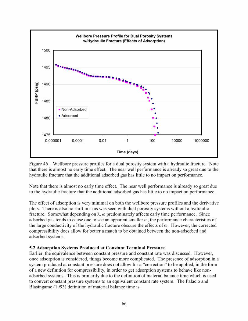
66
Wellbore Pressure Profile for Dual Porosity Systems
w/Hydraulic Fracture (Effects of Adsorption)
1475
1480
1485
1490
1495
1500
0.000001 0.0001 0.01 1 100 10000 1000000
Time (days)
FBHP (psig)
Non-Adsorbed
Adsorbed
Figure 46 – Wellbore pressure profiles for a dual porosity system with a hydraulic fracture. Note
that there is almost no early time effect. The near well performance is already so great due to the
hydraulic fracture that the additional adsorbed gas has little to no impact on performance.
Note that there is almost no early time effect. The near well performance is already so great due
to the hydraulic fracture that the additional adsorbed gas has little to no impact on performance.
The effect of adsorption is very minimal on both the wellbore pressure profiles and the derivative
plots. There is also no shift in ω as was seen with dual porosity systems without a hydraulic
fracture. Somewhat depending on λ, ω predominately affects early time performance. Since
adsorbed gas tends to cause one to see an apparent smaller ω, the performance characteristics of
the large conductivity of the hydraulic fracture obscure the effects of ω. However, the corrected
compressibility does allow for better a match to be obtained between the non-adsorbed and
adsorbed systems.
5.2 Adsorption Systems Produced at Constant Terminal Pressure
Earlier, the equivalence between constant pressure and constant rate was discussed. However,
once adsorption is considered, things become more complicated. The presence of adsorption in a
system produced at constant pressure does not allow for a “correction” to be applied, in the form
of a new definition for compressibility, in order to get adsorption systems to behave like non-
adsorbed systems. This is primarily due to the definition of material balance time which is used
to convert constant pressure systems to an equivalent constant rate system. The Palacio and
Blasingame (1993) definition of material balance time is

67
Type Curves for Dual Porosity Systems w/Hydraulic Fractures
(Constant Rate) (Effects of Adsorption)
0.01
0.1
1
10
100
1000
10000
0.01 0.1 1 10 100 1000 10000 100000 100000
0
1E+07 1E+08
td
pwd or td*ln(pwd)/dtd
PwdNon-AdsorbedAdsorbed Gas-Not Corrected
Adsorbed Gas-Corrected
Figure 47 – Diagnostic plot for dual porosity systems with a hydraulic fracture. Again, note that
there is almost no early time effect of adsorption. There is also no shift in omega as was seen
with dual porosity systems without a hydraulic fracture. Somewhat depending on lambda,
omega is predominately affects early time performance. Since adsorbed gas tends to cause one
to see an apparent smaller omega, the huge conductivity of the hydraulic fracture counteracts
this.
∫
−=
t
tg
g
i
i
g
tigia dt
dt
dp
pcp
c
z
p
p
Gz
q
ct
0 )()(µ
µ
Eq 119
The only assumption made so far is that the single-phase, gas material balance equation applies.
This requires that the reservoir be volumetric and the only source of energy for production come
from gas expansion. This begs the question of whether or not it would be meaningful to
introduce the new definition of compressibility into G (original gas in place). It would be
meaningful, but it would not change the definition of ta since Gi is a constant and is removed
from any integral expression.
The next step in computing ta is typically to assume that total system compressibility (ct) is equal
to gas compressibility (cg). For non-adsorbed systems, this is usually a reasonable assumption.
For systems with significant amounts of adsorbed gas, this represents a serious error in two
ways. The first error being that total system compressibility is now most accurately represented

68
by the equation for ct from Spivey and Semmelbeck (1995). This new ct is in no way equal to cg
for reservoirs with large amounts of adsorbed gas. So, ct and cg should be left inside the integral
which will require an iterative solution. Since the solution is already iterative, these additional
calculations require only a minimal amount of additional effort.
The second error that is referred to above is the indirect result of compressibility being removed
from the pressure integral. Recall that production data analysis is frequently done using the
dimensionless time variable (tda) as the x-axis plotting function. The equation for tda is (Cox, et
al. 2002)
Ac
ktt
it
da φµ )(= Eq 120
To incorporate material balance time, substituted at for t where
( ))()(2
pmpmp
Gz
q
ct i
i
i
g
tigia −
=µ
Eq 121
Combining and simplifying
g
i
i
ida
q
pmpm
A
kG
p
zt
)]()([
2
−=
φ
Eq 122
The equation given above is what is typically plotted on the x-axis. It is apparent that
compressibility is no longer in the equation for tda in the traditional evaluation. So, this brings to
light a very important point. It appears that any attempt to account for the behavior of systems
that have significant amounts of adsorbed gas is futile in dimensionless space with the new
definition of compressibility that was proposed by Bumb and McKee (1988) and Spivey and
Semmelbeck (1995). That is not to say that the definition is incorrect. Spivey and Semmelbeck
(1995) showed that it worked quite well for systems when the rate-time analysis was done in
real/dimensional space. It is simply that compressibility is not in the equation for tda.
However, it was shown earlier that one of the assumptions that is typically used in the
development of ta is incorrect for adsorbed systems. If this assumption is not made, then the
definitions of ta and tda are
∫
−=
t
tg
g
i
i
g
tigia dt
dt
dp
pcp
c
z
p
p
Gz
q
ct
0 )()(µ
µ
Eq 123

69
newda
g
ctict
i
i
da tq
pmpm
A
kG
p
zt =
−=
)]()([
2 φ
Eq 124
Eq 124 for tdanew does not make the assumption that allows compressibility to be eliminated from
the integral. This new integral is essentially pseudopressure with the ratio (cg/ct) left inside.
This new integral is represented with the group ))()(( pmpm ctict − .
Figure 48 and Figure 49 are intended to show the effects of adsorbed gas on a dual porosity
system. All of the models used to generate the datasets are identical to the dual porosity models
presented earlier except that these are produced at a constant flowing bottomhole pressure and
they contain adsorbed gas. All of the datasets were converted to constant rate using the modified
material balance time function described above.
Rate-Decline Type Curves for Dual Porosity Systems
(Effects of Adsorption)
0.000001
0.00001
0.0001
0.001
0.01
0.00001 0.0001 0.001 0.01 0.1 1 10 100 1000 10000
time (days)
qg/(m(pi)-m(pwf))
Adsorbed System
Non-Adsorbed System
Figure 48 – Rate-decline type curves for dual porosity systems showing the effects of adsorption.
Note that the majority of the effect comes at late-time (i.e. lower pressure).
The effect of adsorption on dual porosity systems produced at constant pressure is the same as
those produced at constant rate and can be seen in Figure 48 and Figure 49. This is to be
expected since the equivalence of the systems was shown earlier. Adsorption results in a smaller
“apparent” ω and a horizontal shift of the type curve.
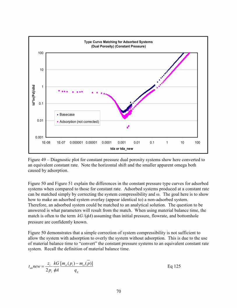
70
Type Curve Matching for Adsorbed Systems
(Dual Porosity) (Constant Pressure)
0.001
0.01
0.1
1
10
100
1E-08 1E-07 0.000001 0.00001 0.0001 0.001 0.01 0.1 1 10 100
tda or tda_new
td*ln(Pd)/dtd
Basecase
Adsorption (not corrected)
Figure 49 – Diagnostic plot for constant pressure dual porosity systems show here converted to
an equivalent constant rate. Note the horizontal shift and the smaller apparent omega both
caused by adsorption.
Figure 50 and Figure 51 explain the differences in the constant pressure type curves for adsorbed
systems when compared to those for constant rate. Adsorbed systems produced at a constant rate
can be matched simply by correcting the system compressibility and ω. The goal here is to show
how to make an adsorbed system overlay (appear identical to) a non-adsorbed system.
Therefore, an adsorbed system could be matched to an analytical solution. The question to be
answered is what parameters will result from the match. When using material balance time, the
match is often to the term )/( AkG φ assuming than initial pressure, flowrate, and bottomhole
pressure are confidently known.
Figure 50 demonstrates that a simple correction of system compressibility is not sufficient to
allow the system with adsorption to overly the system without adsorption. This is due to the use
of material balance time to “convert” the constant pressure systems to an equivalent constant rate
system. Recall the definition of material balance time.
g
ctict
i
ida
q
pmpm
A
kG
p
znewt
)]()([
2
−=
φ
Eq 125
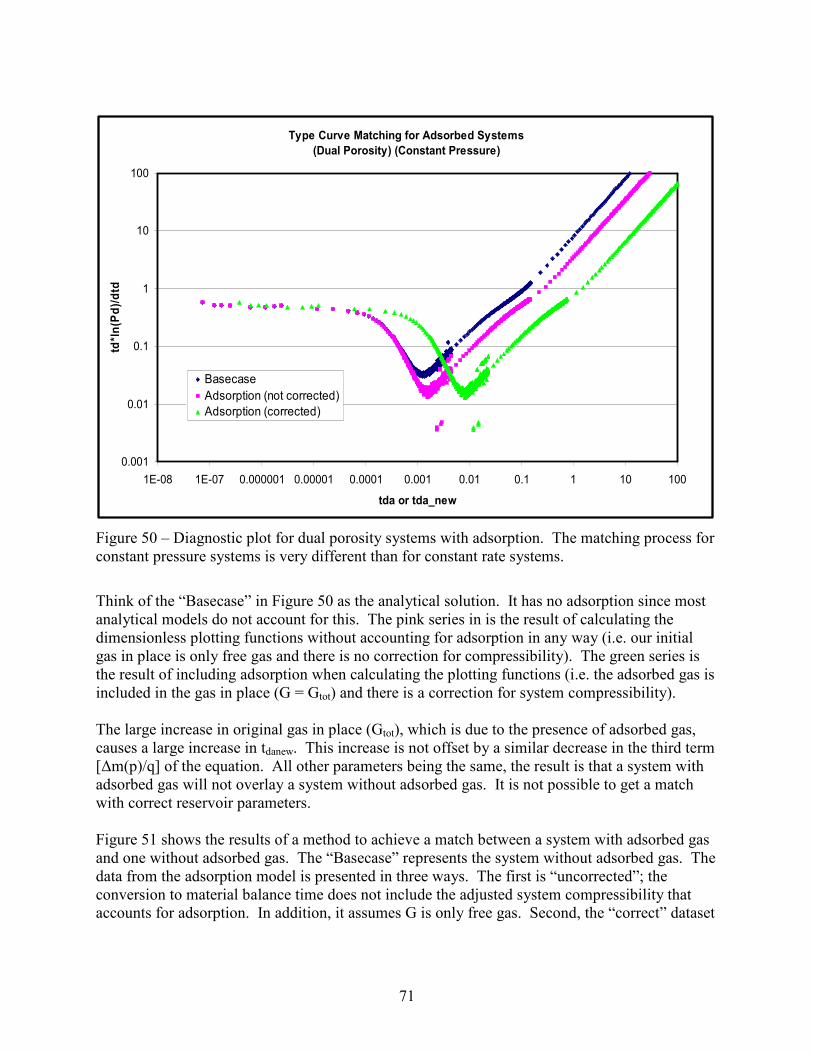
71
Type Curve Matching for Adsorbed Systems
(Dual Porosity) (Constant Pressure)
0.001
0.01
0.1
1
10
100
1E-08 1E-07 0.000001 0.00001 0.0001 0.001 0.01 0.1 1 10 100
tda or tda_new
td*ln(Pd)/dtd
Basecase
Adsorption (not corrected)
Adsorption (corrected)
Figure 50 – Diagnostic plot for dual porosity systems with adsorption. The matching process for
constant pressure systems is very different than for constant rate systems.
Think of the “Basecase” in Figure 50 as the analytical solution. It has no adsorption since most
analytical models do not account for this. The pink series in is the result of calculating the
dimensionless plotting functions without accounting for adsorption in any way (i.e. our initial
gas in place is only free gas and there is no correction for compressibility). The green series is
the result of including adsorption when calculating the plotting functions (i.e. the adsorbed gas is
included in the gas in place (G = Gtot) and there is a correction for system compressibility).
The large increase in original gas in place (Gtot), which is due to the presence of adsorbed gas,
causes a large increase in tdanew. This increase is not offset by a similar decrease in the third term
[∆m(p)/q] of the equation. All other parameters being the same, the result is that a system with
adsorbed gas will not overlay a system without adsorbed gas. It is not possible to get a match
with correct reservoir parameters.
Figure 51 shows the results of a method to achieve a match between a system with adsorbed gas
and one without adsorbed gas. The “Basecase” represents the system without adsorbed gas. The
data from the adsorption model is presented in three ways. The first is “uncorrected”; the
conversion to material balance time does not include the adjusted system compressibility that
accounts for adsorption. In addition, it assumes G is only free gas. Second, the “correct” dataset

72
Type Curve Matching for Adsorbed Systems
(Dual Porosity) (Constant Pressure)
0.001
0.01
0.1
1
10
100
1E-08 1E-07 0.000001 0.00001 0.0001 0.001 0.01 0.1 1 10 100
tda or tda_new
td*ln(Pd)/dtd
BasecaseAdsorption (not corrected)Adsorption (corrected)Match Dataset
Figure 51 – Diagnostic plot for dual porosity systems produced at constant pressure shown here
converted to an equivalent constant rate. The “Match Dataset” represents the system with the
parameters necessary to overlay an analytical solution without adsorption.
uses the correction for adsorption and assumes G = Gtot. The match is achieved by using the
adjusted system compressibility and taking G to be only the free gas, not the sum of free gas and
adsorbed gas. This method will allow a match to correct reservoir parameters but to an
“incorrect” gas in place. It should be noted that the match is only to the term )/( AkG φ , assuming
that pi, qg, and pwf are accurately known. Therefore, one must be very sure of the other three
parameters (pi, qg, and pwf) in the above term to come away with the correct match. A summary
of the match terms for the datasets in Figure 51 can be seen in Table 8.
Table 8 – Matching results for dual porosity systems with adsorption.
Basecase Adsorbed System
(not corrected)**
Adsorbed System
(corrected) Match Dataset
)/( AkGi φ 0.2 0.2 2.24 0.2
**Does not overlay the “Basecase” because the third term of tdanew does not include the adjusted
system compressibility for an adsorbed system. Thus, it is too large. Therefore, any overlay of
uncorrected production data to an analytical solution will result in an incorrect match
term )/( AkG φ .**

73
Table 8 seems to indicate that the “Adsorbed System (not corrected)” attained a correct match
since the match term )/( AkG φ is identical to the “Basecase” match term. However, it does not
overlay the “Basecase” because the third term of tdanew does not include the adjusted system
compressibility for an adsorbed system. Thus, it is too large. Therefore, any overlay of
uncorrected production data to an analytical solution will result in an incorrect match term
)/( AkG φ . This highlights the importance of knowing pi, qg, and pwf before embarking on this
type of analysis.
Figure 52 and Figure 53 refers to hydraulically fractured systems with adsorbed gas that were
produced at constant pressure. The same method that was applied to dual porosity systems will
be applied to these systems. However, tda is different for these systems, so the match will be to a
different set of terms. The equation for tda is
g
ctictmf
i
idA
q
pmpm
A
Gk
w
x
p
zt
)]()([01002.0
−=
φ Eq 126
Rate-Decline Type Curves for Hydraulically Fractured Systems
(Effects of Adsorption)
0.0000001
0.000001
0.00001
0.0001
0.001
1E-05 0.0001 0.001 0.01 0.1 1 10 100 1000 10000 100000Time (days)
qg/[m(pi)-m(pwf)]
Non-Adsorbed
Adsorbed
Figure 52 – Rate-decline type curve for a hydraulically fractured system with adsorbed gas
produced at constant pressure. Note again that the effect of adsorption is predominately at late
time.

74
Type Curve Matching for Adsorbed Systems
(Constant Pressure) (Hydraulic Fracture)
0.01
0.1
1
10
100
0.000001 0.00001 0.0001 0.001 0.01 0.1 1 10 100 1000 10000
tda
pwd or tda*ln(p
wd)/dtda
PwdNon-Adsorbed
Adsorbed-CorrectedAdsorbed-Not CorrectedMatch Dataset
Figure 53 – Diagnostic plot for hydraulically fractured systems with adsorbed gas produced at
constant pressure. Shown here converted to an equivalent constant rate system. Note that the
“Adsorbed-Corrected” system does not overlay the “Non-Adsorbed” basecase system since it the
plotting functions were calculated using total gas in place rather than just free gas in place.
Just like before, the uncorrected adsorbed system will not overly the non-adsorbed system if the
correct reservoir properties are used. Recall that there is no difference between the adsorbed and
non-adsorbed cases except for the presence of adsorption. When the correction for adsorption is
applied, the derivative curve shifts sharply to the right due to the much larger original gas in
place (caused by adsorbed gas). Assuming that, pi, qg, and pwf are accurately known, the match
term is )/( AwkGx f φ . The “Match Dataset” is achieved by again taking Gi to be only the free gas
in the adsorbed system instead of the sum of the adsorbed and free gas.
Finally, the effects of adsorption on dual porosity systems with hydraulic fractures will be
documented. Figure 54 shows rate profiles that were generated from a model which was run at
constant terminal pressure rather than constant rate. As has been shown for the systems
examined previously, constant pressure systems must be handled differently than constant rate
systems when production data analysis is performed. The model used to generate the following
rate profiles is identical to that used before for this type of system except that it now contains
adsorbed gas. The dimensionless time plotting functions used in Figure 55 is
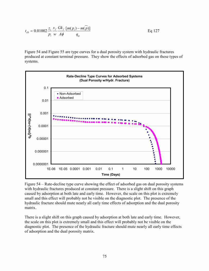
75
g
iff
i
idA
q
pmpm
A
Gk
w
x
p
zt
)]()([01002.0
−=
φ Eq 127
Figure 54 and Figure 55 are type curves for a dual porosity system with hydraulic fractures
produced at constant terminal pressure. They show the effects of adsorbed gas on these types of
systems.
Rate-Decline Type Curves for Adsorbed Systems
(Dual Porosity w/Hydr. Fracture)
0.0000001
0.000001
0.00001
0.0001
0.001
0.01
0.1
1E-06 1E-05 0.0001 0.001 0.01 0.1 1 10 100 1000 10000
Time (Days)
qg/[m(p
i)-m(p
wf)]
Non-Adsorbed
Adsorbed
Figure 54 – Rate-decline type curve showing the effect of adsorbed gas on dual porosity systems
with hydraulic fractures produced at constant pressure. There is a slight shift on this graph
caused by adsorption at both late and early time. However, the scale on this plot is extremely
small and this effect will probably not be visible on the diagnostic plot. The presence of the
hydraulic fracture should mute nearly all early time effects of adsorption and the dual porosity
matrix.
There is a slight shift on this graph caused by adsorption at both late and early time. However,
the scale on this plot is extremely small and this effect will probably not be visible on the
diagnostic plot. The presence of the hydraulic fracture should mute nearly all early time effects
of adsorption and the dual porosity matrix.
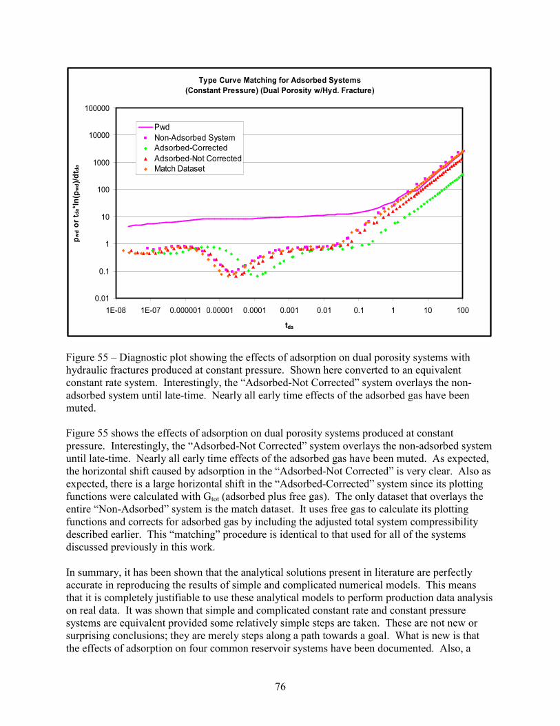
76
Type Curve Matching for Adsorbed Systems
(Constant Pressure) (Dual Porosity w/Hyd. Fracture)
0.01
0.1
1
10
100
1000
10000
100000
1E-08 1E-07 0.000001 0.00001 0.0001 0.001 0.01 0.1 1 10 100
tda
pwd or t da*ln(p
wd)/dt da
Pwd
Non-Adsorbed System
Adsorbed-Corrected
Adsorbed-Not Corrected
Match Dataset
Figure 55 – Diagnostic plot showing the effects of adsorption on dual porosity systems with
hydraulic fractures produced at constant pressure. Shown here converted to an equivalent
constant rate system. Interestingly, the “Adsorbed-Not Corrected” system overlays the non-
adsorbed system until late-time. Nearly all early time effects of the adsorbed gas have been
muted.
Figure 55 shows the effects of adsorption on dual porosity systems produced at constant
pressure. Interestingly, the “Adsorbed-Not Corrected” system overlays the non-adsorbed system
until late-time. Nearly all early time effects of the adsorbed gas have been muted. As expected,
the horizontal shift caused by adsorption in the “Adsorbed-Not Corrected” is very clear. Also as
expected, there is a large horizontal shift in the “Adsorbed-Corrected” system since its plotting
functions were calculated with Gtot (adsorbed plus free gas). The only dataset that overlays the
entire “Non-Adsorbed” system is the match dataset. It uses free gas to calculate its plotting
functions and corrects for adsorbed gas by including the adjusted total system compressibility
described earlier. This “matching” procedure is identical to that used for all of the systems
discussed previously in this work.
In summary, it has been shown that the analytical solutions present in literature are perfectly
accurate in reproducing the results of simple and complicated numerical models. This means
that it is completely justifiable to use these analytical models to perform production data analysis
on real data. It was shown that simple and complicated constant rate and constant pressure
systems are equivalent provided some relatively simple steps are taken. These are not new or
surprising conclusions; they are merely steps along a path towards a goal. What is new is that
the effects of adsorption on four common reservoir systems have been documented. Also, a

77
matching procedure has been outlined that allows a real production dataset from a reservoir that
has adsorbed gas to be matched to an analytical model. This matching procedure required the
modification of existing methodology to adapt to the complexities of adsorbed systems. Next,
this procedure will be applied to actual field datasets to examine its viability, strengths, and
shortcomings.

78
6. TRIAL CASES
The effects of adsorption have been documented on production data type curves. In addition, a
new definition of material balance time has been proposed that prevents system compressibility
from being eliminated in the dimensionless plotting function tdanew. Thus, the effects of
adsorption can now be better accounted for when using dimensionless plotting functions for
production data analysis.
6.1 Simulation Example Well
This next discussion will explain how the techniques described previously are applied in
production data analysis. For this discussion, a simulated dataset will be used so that data
reliability and accuracy do not cause problems (the model will be discussed later). The
methodology for matching production data to an analytical, type curve solution will be
discussed. However, an analyst rarely has a complete understanding of the reservoir in question
when the analysis of the production data is performed. So, the same set of production data will
be analyzed using different analytical models (single porosity, dual porosity, and dual porosity
w/hydraulic fracture). The effect of these different analysis styles will be noted in the match
parameters. The important question being whether or not any additional insight is gained from
using a more complicated model.
In addition, the effects on match parameters of correcting system compressibility to account for
adsorbed gas will be investigated. Is it really necessary to correct for adsorption when using the
various analytical models? If so, what mistakes are made when adsorbed gas is not accounted
for?
Shale gas systems were described in detail earlier. Presently, reservoir descriptions of common
shale gas reservoirs are considered to be dual porosity reservoirs with adsorbed gas in the matrix
portion only. In addition, shale gas wells are typically stimulated by hydraulic fracturing.
Therefore, the simulation model used for this section is a representation of these features.
Production comes from a single well located in the center of the model which can be seen in
Figure 56. Local grid refinement was used to create the hydraulic fracture, and resulted in a
fracture width of 4 inches. Aerial views of the grid that show the local grid refinement can be
seen in Figure 23. The reservoir parameters can be found in Table 9 and the relative
permeability curves can be found in Figure 57 and Figure 58.
Lastly, the rate profile generated by the simulation model is shown in Figure 59. The flowing
bottomhole pressure was set at 914 psia to achieve starting rates close to 1 MMSCF/day. The
model was run for 10 years with daily production data being recorded for the first 3 months
followed by monthly data points for the remaining time. This same rate profile will be analyzed
with the various types of analytical models mentioned before in Chapter 4 and Chapter 5.
6.1.1 Analysis as a Single Porosity System with Adsorbed Gas
The most common system used in production data analysis is a single porosity system because
these reservoirs are very common and relatively simple to analyze. So, in this analysis, 3
different styles of type curves will be used. First, a plot of qd vs. td will be analyzed to determine
a match. Second, a Fetkovich plot will be used which plots qDd vs tDd. Lastly, a plot of pwd vs.

79
Table 9 – Simulation Example Well Dataset
Height/Net Pay (ft) 40
Length (x & y) (ft) 5280
Well Radius, rw (ft) 0.25
Porosity, mφ 0.10
Porosity, fφ 0.001 (ω = 0.01)
xf (ft) 480 (Cdf = 0.03)
Permeability, km(md) 0.01
Permeability, kf(md) 1.875 (λ = 1x10⁻⁵)
Permeability, kfh(md) 2500 (Cdf = 0.3)
Initial Pressure, (psia) 1514
Water Saturation, Sw 0.05
Rock Dens., (g/cm3) 2.45
pL (psia) 635
vL (scf/ton) 89
Temperature, (oF) 225
Gas Gravity 0.6
Gas Composition 100% CH4
Initial BHP (psia) 914
Figure 56 – Depiction of Simulation
Example Well Model
Figure 57 – Oil-Water Relative Permeability Curve for Simulation Example Well
Well Fracture
40 ft
5280 ft
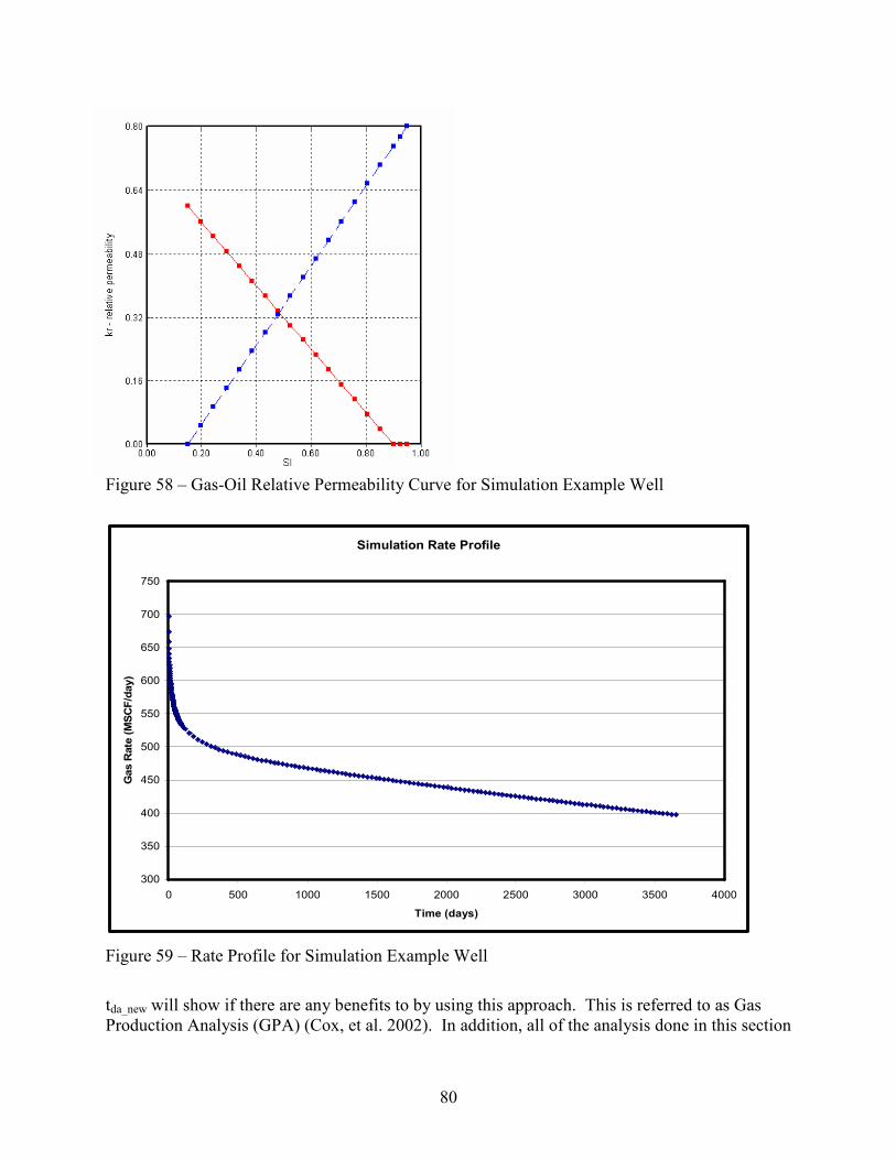
80
Figure 58 – Gas-Oil Relative Permeability Curve for Simulation Example Well
Figure 59 – Rate Profile for Simulation Example Well
tda_new will show if there are any benefits to by using this approach. This is referred to as Gas
Production Analysis (GPA) (Cox, et al. 2002). In addition, all of the analysis done in this section
Simulation Rate Profile
300
350
400
450
500
550
600
650
700
750
0 500 1000 1500 2000 2500 3000 3500 4000
Time (days)
Gas Rate (MSCF/day)

81
will treat the models as if adsorbed gas is present and correct for it. The next section will detail
the effects of analyzing the system without correcting for adsorbed gas.
It should be noted that the method to achieve the match with the various sets of type curves
mentioned above is different than what is traditionally done. Traditionally, the production data
and/or pressure functions are plotted against a real-time function on one graph and the analytical
dimensionless solutions, or type curves, are plotted on another. These two graphs are overlayed
to achieve a match. This overlay and the resulting match points are used to estimate the reservoir
parameters of interest. Here, the match is achieved by changing reservoir parameters, chiefly
permeability, porosity, and drainage radius, and then converting the rate or pressure data into
dimensionless format to obtain a match. So, every time one of these parameters is changed the
plotting functions are recalculated to reflect this new data. The new plotting functions are then
plotted against the analytical dimensionless solution for the model of interest (for example, a
single porosity analytical solution) to obtain a match. A similar recalculation procedure is also
required for all methods that involve material balance time.
In this particular case, a dual porosity system with hydraulic fractures is being simplified since it
is being viewed as a single porosity system. So, all the properties for both natural and man-made
fractures influence the rates obtained from the flow simulation, but do not appear in the
conversion of the data into dimensionless format. First, the outcome of the qd vs. td will be
examined. The values of all of the relevant parameters were changed until an appropriate match
was obtained to a single porosity analytical solution type curve. The values in Table 10 are the
values that were matched to the single porosity analytical solution.
Table 10 – qd vs. td match results for single porosity system with adsorbed gas
sg = 0.6
re = 2640 ft
rw = 0.25 ft
A = 2.79E+07 ft^2
h = 40 ft
vb = 1.12E+09 ft^3
sw = 0.05 fraction
phi = 0.15 fraction
tres = 225 oF
pi = 1514.70 psia
pL = 635 psia ρm = 2.45 g/cm^3
vL = 89 scf/ton 6.81 scf/ft^3
z = 0.929
bgi = 0.012 rcf/scf 2.117 rbbl/mscf
OGIPfree = 13374898 MSCF
OGIPads = 4545700 MSCF
Total = 17920598 MSCF G/A = 0.48
km (md) = 1.15 km (nd) = 1150000
INITIAL DATA
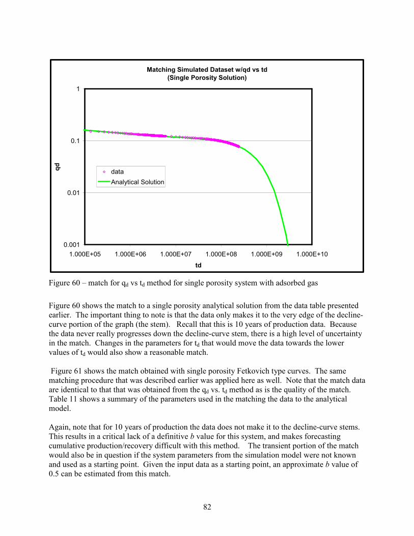
82
Matching Simulated Dataset w/qd vs td
(Single Porosity Solution)
0.001
0.01
0.1
1
1.000E+05 1.000E+06 1.000E+07 1.000E+08 1.000E+09 1.000E+10
td
qd
data
Analytical Solution
Figure 60 – match for qd vs td method for single porosity system with adsorbed gas
Figure 60 shows the match to a single porosity analytical solution from the data table presented
earlier. The important thing to note is that the data only makes it to the very edge of the decline-
curve portion of the graph (the stem). Recall that this is 10 years of production data. Because
the data never really progresses down the decline-curve stem, there is a high level of uncertainty
in the match. Changes in the parameters for td that would move the data towards the lower
values of td would also show a reasonable match.
Figure 61 shows the match obtained with single porosity Fetkovich type curves. The same
matching procedure that was described earlier was applied here as well. Note that the match data
are identical to that that was obtained from the qd vs. td method as is the quality of the match.
Table 11 shows a summary of the parameters used in the matching the data to the analytical
model.
Again, note that for 10 years of production the data does not make it to the decline-curve stems.
This results in a critical lack of a definitive b value for this system, and makes forecasting
cumulative production/recovery difficult with this method. The transient portion of the match
would also be in question if the system parameters from the simulation model were not known
and used as a starting point. Given the input data as a starting point, an approximate b value of
0.5 can be estimated from this match.

83
Matching Simulated Dataset w/Fetkovich
(Single Porosity Solution)
0.010
0.100
1.000
10.000
0.001 0.01 0.1 1 10 100
tDd
qDd
rd = 10000rd = 1000rd = 100b = 0.1b = 0.25b = 0.5b = 0.75b = 1Data
Figure 61 – match for Fetkovich method for single porosity system with adsorbed gas
Table 11 shows a summary of the match data for the GPA method. There are some differences
between this match data and that obtained from the previous two methods. Chiefly, the drainage
radius and porosity obtained from this match are correct when they are compared to the
simulator input data. There is also a very slight difference in the permeability obtained from the
previous two methods when compared to this method, but that can be considered negligible.
Figure 62 shows the match achieved using the GPA method with a single porosity analytical
solution. Boundary-dominated flow is clearly reached which makes the match much more
reliable and useful.
There are some common observations that apply to all of these plots. Since this system was
assumed to be a single porosity system when it is actually a dual porosity system with hydraulic
fractures, the very early time behavior will not overlay the type curves. However, it was shown
previously that the only parameter obtained from very early time behavior is ω. It was also
shown that the bottomhole pressure drop over which this parameter is obtained is very small
(<10 psi) for the dual porosity systems of interest. In reality, bottomhole pressures are usually
obtained from multiphase flow correlations using tubing head pressure and fluid composition.
Since the accuracy of real production data, especially tubing head pressures, is rarely less than 10
psi, it is doubtful that ω could ever be obtained with any certainty for this particular system.

84
Matching Simulated Dataset w/GPA
(Single Porosity Solution)
0.1
1.0
10.0
100.0
1.00E+04 1.00E+05 1.00E+06 1.00E+07 1.00E+08 1.00E+09
tda_new
pwd or pwd'
Pwd
Pwd'
Analytical Solution
Figure 62 – match for GPA for single porosity system with adsorbed gas
Another observation common to the different analyses is that the permeability obtained is neither
matrix permeability nor fracture permeability. This is to be expected since this system is
incorrectly assumed to behave as a single porosity system.
Table 11 is a summary of the matching results achieved by the various styles of type curves that
were used.
Table 11 – Summary of matching results for single porosity system with adsorbed gas
Drainage
radius, re (ft)
Porosity
( mφ ) Eff. Sysetm
Permeability, k (md) G/A*
Match Term
( AkG φ )
qd vs td 3000 0.15 1.2 0.48 n/a
Fetkovich 3000 0.15 1.2 0.48 n/a
GPA (pwd vs tda_new) 2640 0.15 1.15 0.48 3.68
Actual (from model) 2640 0.1 1.8 (kf), 0.01 (km) 0.32 5.76**
*Using free gas only. G/A with adsorbed gas is 0.49 for the model and 0.64 for the matches*
** based on kf **
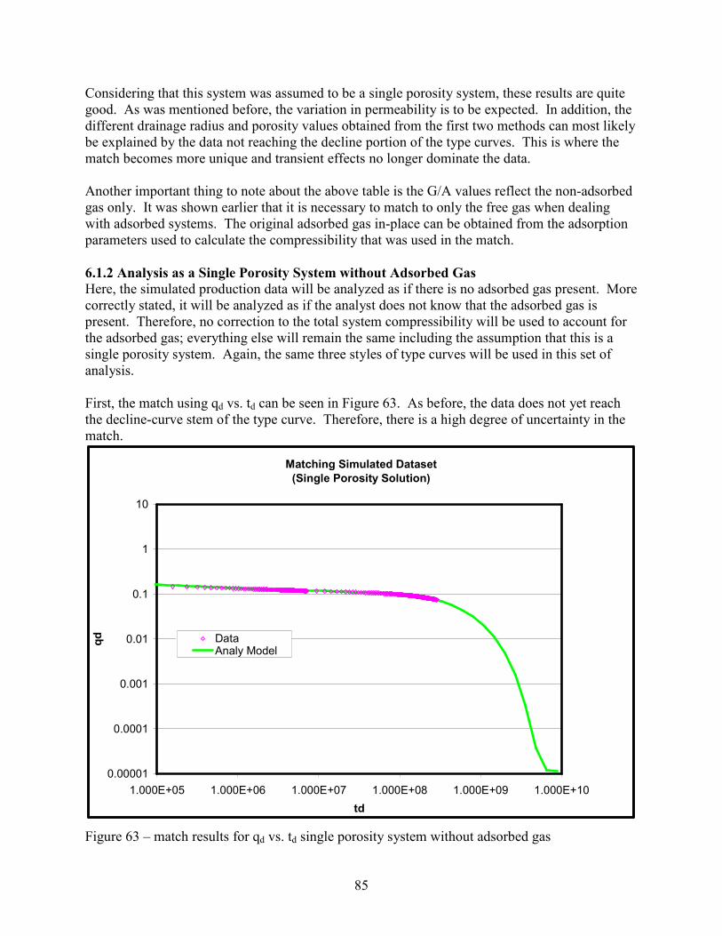
85
Considering that this system was assumed to be a single porosity system, these results are quite
good. As was mentioned before, the variation in permeability is to be expected. In addition, the
different drainage radius and porosity values obtained from the first two methods can most likely
be explained by the data not reaching the decline portion of the type curves. This is where the
match becomes more unique and transient effects no longer dominate the data.
Another important thing to note about the above table is the G/A values reflect the non-adsorbed
gas only. It was shown earlier that it is necessary to match to only the free gas when dealing
with adsorbed systems. The original adsorbed gas in-place can be obtained from the adsorption
parameters used to calculate the compressibility that was used in the match.
6.1.2 Analysis as a Single Porosity System without Adsorbed Gas
Here, the simulated production data will be analyzed as if there is no adsorbed gas present. More
correctly stated, it will be analyzed as if the analyst does not know that the adsorbed gas is
present. Therefore, no correction to the total system compressibility will be used to account for
the adsorbed gas; everything else will remain the same including the assumption that this is a
single porosity system. Again, the same three styles of type curves will be used in this set of
analysis.
First, the match using qd vs. td can be seen in Figure 63. As before, the data does not yet reach
the decline-curve stem of the type curve. Therefore, there is a high degree of uncertainty in the
match.
Matching Simulated Dataset
(Single Porosity Solution)
0.00001
0.0001
0.001
0.01
0.1
1
10
1.000E+05 1.000E+06 1.000E+07 1.000E+08 1.000E+09 1.000E+10
td
qd Data
Analy Model
Figure 63 – match results for qd vs. td single porosity system without adsorbed gas

86
The visual quality of the match is the same as it was when adsorption was considered in the
matching process, and the drainage radius that was obtained from this match is also the same as
what was obtained previously when system compressibility was corrected for adsorption. A
summary of the results from this match can be seen in Table 12.
Second, the results from the Fetkovich style type curve analysis can be seen in Figure 64. Again,
the data does not yet reach the decline-curve portion of the type curve. Therefore, there is a high
degree of uncertainty, and no b value can be obtained yet.
Fetkovich Single Porosity Type Curves
0.01
0.10
1.00
10.00
0.001 0.01 0.1 1 10 100
tDd
qDd
rd = 10000rd = 1000rd = 100b = 0.1b = 0.25b = 0.5b = 0.75b = 1Data
Figure 64 – match for Fetkovich method for single porosity systems without adsorbed gas
As with the qd vs. td type curve, the drainage radius obtained from this match is the same as what
was obtained when adsorption was accounted for, and the quality of the match is also the same as
before. A summary of the results from this match can be seen in Table 12.
Lastly, GPA was used to analyze the data, and the results can be seen in Figure 65. The data still
reaches the boundary-dominated portion of the type curve. As expected, not accounting for
adsorption has no effect on whether or not the data reaches this flow regime.
The match quality is the same as it was when adsorption was accounted for. The drainage radius
obtained is the same as it was when adsorption was not accounted for. A summary of the results
from this match can be seen in Table 12.

87
Matching Simulated Dataset w/GPA
(Single Porosity Solution)
0.1
1.0
10.0
100.0
1.00E+04 1.00E+05 1.00E+06 1.00E+07 1.00E+08 1.00E+09
tda
pwd or pwd'
Pwd
Pwd'
Analytical Solution
Figure 65 – match for GPA method for single porosity system without adsorbed gas
Table 12 – Summary of matching results for single porosity systems without adsorbed gas
Drainage
radius, re (ft)
Porosity
( mφ ) Eff. Sysetm
Permeability, k (md) G/A*
Match Term
( AkG φ ) *
qd vs td 3000 0.15 1.19 0.48 n/a
Fetkovich 3000 0.15 1.19 0.48 n/a
GPA no adsorp. 2640 0.15 1.15 0.48 3.68
GPA w/adsorp. 2640 0.15 1.15 0.48 3.68
Actual (from model) 2640 0.1 1.8 (kf), 0.01 (km) 0.32 5.76**
*Using free gas only. G/A with adsorbed gas is 0.49 for the model and 0.64 for the matches.
But it is not possible to obtain this from this analysis since the correction for compressibility was
not used. Therefore, pL and vL cannot be verified *
**Using fracture permeability**
Table 12 can be used to compare the results of using the correction for adsorption and not using
it. The theoretical benefit of using the correction for compressibility to account for adsorption is
it allows the analyst to determine the adsorption properties and thus the volume of adsorbed gas.
However, it was shown that the shift caused by adsorption when adsorption properties for the
Barnett Shale are used is not detectable. This is due to the placement of vL and pL in the equation
for total system compressibility which can be seen in Eq 102. The effects of adsorption on
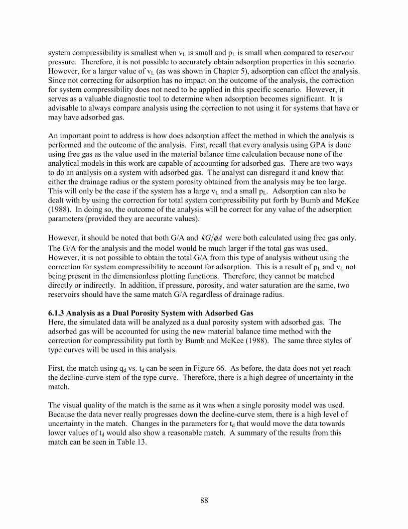
88
system compressibility is smallest when vL is small and pL is small when compared to reservoir
pressure. Therefore, it is not possible to accurately obtain adsorption properties in this scenario.
However, for a larger value of vL (as was shown in Chapter 5), adsorption can effect the analysis.
Since not correcting for adsorption has no impact on the outcome of the analysis, the correction
for system compressibility does not need to be applied in this specific scenario. However, it
serves as a valuable diagnostic tool to determine when adsorption becomes significant. It is
advisable to always compare analysis using the correction to not using it for systems that have or
may have adsorbed gas.
An important point to address is how does adsorption affect the method in which the analysis is
performed and the outcome of the analysis. First, recall that every analysis using GPA is done
using free gas as the value used in the material balance time calculation because none of the
analytical models in this work are capable of accounting for adsorbed gas. There are two ways
to do an analysis on a system with adsorbed gas. The analyst can disregard it and know that
either the drainage radius or the system porosity obtained from the analysis may be too large.
This will only be the case if the system has a large vL and a small pL. Adsorption can also be
dealt with by using the correction for total system compressibility put forth by Bumb and McKee
(1988). In doing so, the outcome of the analysis will be correct for any value of the adsorption
parameters (provided they are accurate values).
However, it should be noted that both G/A and AkG φ were both calculated using free gas only.
The G/A for the analysis and the model would be much larger if the total gas was used.
However, it is not possible to obtain the total G/A from this type of analysis without using the
correction for system compressibility to account for adsorption. This is a result of pL and vL not
being present in the dimensionless plotting functions. Therefore, they cannot be matched
directly or indirectly. In addition, if pressure, porosity, and water saturation are the same, two
reservoirs should have the same match G/A regardless of drainage radius.
6.1.3 Analysis as a Dual Porosity System with Adsorbed Gas
Here, the simulated data will be analyzed as a dual porosity system with adsorbed gas. The
adsorbed gas will be accounted for using the new material balance time method with the
correction for compressibility put forth by Bumb and McKee (1988). The same three styles of
type curves will be used in this analysis.
First, the match using qd vs. td can be seen in Figure 66. As before, the data does not yet reach
the decline-curve stem of the type curve. Therefore, there is a high degree of uncertainty in the
match.
The visual quality of the match is the same as it was when a single porosity model was used.
Because the data never really progresses down the decline-curve stem, there is a high level of
uncertainty in the match. Changes in the parameters for td that would move the data towards
lower values of td would also show a reasonable match. A summary of the results from this
match can be seen in Table 13.

89
Second, the results from the Fetkovich style type curve analysis can be seen in Figure 67. Again,
the data does not yet reach the decline-curve portion of the type curve. Therefore, there is a high
degree of uncertainty, and no b value can be obtained yet.
Matching Simulation Dataset
(Dual Porosity)
0.001
0.01
0.1
1
1.00E+02 1.00E+03 1.00E+04 1.00E+05 1.00E+06 1.00E+07 1.00E+08 1.00E+09 1.00E+10
td
qd
Analy. Solution
Sim Data (qd)
Figure 66 – match qd vs. td method for dual porosity systems with adsorbed gas.
The visual quality of the match presented in Figure 67 is good. The data just begins to start
down the depletion stems. While it is not possible to give a definitive b value, an approximate
value of 0.25 is indicated. The results from this match can be seen in Table 13.
Lastly, GPA was used to analyze the data, and the results can be seen in Figure 68. The data still
reaches the boundary-dominated portion of the type curve. The match resulting from using a
dual porosity model offers the same visual quality as that of a single porosity model. There is
some indication of what the value of ω might be with the dual porosity model. But, the data does
not go back far enough in time to allow for an accurate determination of ω. The results from this
match can be seen in Table 13.
Table 11 and Table 13 are a good comparison of what benefits can be obtained from using a
more complex analysis. Table 13 presents a summary of the results obtained from “matching”
the simulated dataset to a dual porosity analytical model. The only substantial difference
between Table 11 and Table 13 is the presence of both matrix and fracture permeability.
However, even the dual porosity model does not capture the true fracture permeability. It should

90
be noted that the dual porosity analytical model was developed using an effective total system
permeability. Therefore, any match to the analytical models is obtained using effective system
permeability. Otherwise, this dual porosity model gives almost identical G/A and match term
values as the single porosity case did.
Dual Porosity Fetkovich Type Curves
(rd = 12000)
0.100
1.000
10.000
1E-08 1E-07 1E-06 0.00001 0.0001 0.001 0.01 0.1 1 10
tDd
QDd
Lam=1E-3 Omg=0.001 Lam=1E-5 Omg=0.001Lam=1E-7 Omg=0.001 Lam=1E-3 Omg=0.01Lam=1E-3 Omg=0.1 Lam=1E-5 Omg=0.01Lam=1E-5 Omg=0.1 Lam=1E-7 Omg=0.01Lam=1E-78 Omg=0.1 Datab=0.1 b=0.25b=0.5 b=0.75b=1
Figure 67 – match for Fetkovich method for dual porosity systems with adsorbed gas.
Table 13 – Summary of matching results for dual porosity systems with adsorbed gas.
Drainage
radius, re
(ft)
ω λ G/A* Match Term
( AkG φ ) *
qd vs td 3000 0.01 1 x 10⁻⁵ 0.32 n/a
Fetkovich 3000 0.01 1 x 10⁻⁵ 0.32 n/a
GPA
(pwd vs tda_new) 2640 0.008 1.75 x 10
-5 0.32 3.52
Actual
(from model) 2640 0.01 1 x 10
-5 0.32 5.76**
*Using free gas only. G/A with adsorbed gas is much larger*
**Using fracture permeability**

91
Matching Simulated Dataset w/GPA
(Dual Porosity Solution)
0.01
0.1
1
10
100
1.00E+02 1.00E+03 1.00E+04 1.00E+05 1.00E+06 1.00E+07 1.00E+08 1.00E+09
td and tda_new
pwd'
Analy. Model
Data
Figure 68 – match for GPA method for dual porosity system with adsorbed gas.
6.1.4 Analysis as a Hydraulically Fractured System with Adsorbed Gas
Here, the simulated data will be analyzed as a hydraulically fractured system with adsorbed gas.
The adsorbed gas will be accounted for using the new material balance time method with the
correction for compressibility put forth by Bumb and McKee (1988). Only two analysis styles
were examined for this type of system. GPA and qd vs. td were used, but Fetkovich analysis was
not. The analytical model used for a hydraulically fracture system is not a complete solution. It
has a boundary-dominated (i.e. late-time) model coupled to an early-time hydraulic fracture
model. Based on the results thus far, Fetkovich style analysis does not yield much additional
information because the simulated data does not fall onto the decline portion of the type curves.
First, the match using qd vs. td can be seen in Figure 69. The dashed line is the analytic model
for early-time fracture flow. The solid line is the analytic model for pseudoradial and boundary
dominated flow. As before, the data does not yet reach the decline-curve stem of the type curve.
Therefore, there is a high degree of uncertainty in the match. It should also be noted that that
this data displays no evidence of the early-time hydraulic fracture behavior. Said another way,
this data does not exhibit anywhere near the correct value for Cdf as is indicated by its failure to
follow the early-time hydraulic fracture curve in Figure 69. The results from this match can be
seen in Table 14.

92
Matching Simulated Dataset (Hyd. Fracture)
0.01
0.1
1
10
0.001 0.01 0.1 1 10 100 1000 10000 100000
td/Cdf or tda/Cdf
td*d(lnpd)/dtd
Analy Mode (Frac)l
Analy Model (Lt-Time)
Data
Figure 69 – match using qd vs td for a hydraulically fractured system with adsorbed gas
Lastly, GPA was used to analyze the data, and the results can be seen in Figure 70. The data still
reaches the boundary-dominated portion of the type curve. The match resulting from using a
hydraulic fracture model offers the same visual quality as that of a single porosity or dual
porosity model. In this case, there are a few data points that fall on the early-time hydraulic
fracture curve with the majority falling on the pseudo-radial and late-time portions of the
solution. The results from this match can be seen in Table 14.
Table 14 – Summary of matching data for hydraulically fractured systems with adsorbed gas.
Drainage
radius, re
(ft)
Porosity
(φm)
Matrix
Perm.
(md)
Cdf G/A* Match Term
( AkG φ/ ) *
qd vs td 3000 0.1 1.1 n/a 0.33 n/a
GPA
(pwd vs tda_new) 2640 0.1 1.1 0.4 0.32 3.52
Actual
(from model) 2640 0.1
1.8 (kf)
0.01 (km) 0.3 0.32 5.76**
93
Matching Simulated Dataset
(Hyd. Fracture)
0.01
0.1
1
10
100
1.00E-03 1.00E-02 1.00E-01 1.00E+00 1.00E+01 1.00E+02 1.00E+03 1.00E+04
td/Cdf or tda/Cdf
td*dln(pd)/dtd
Analy Model (Frac)
Analy Model (Lt-Time)
Data
Figure 70 – match using GPA for hydraulically fractured system with adsorbed gas
Figure 70 gives some indication of what the value of Cdf might be with this hydraulic fracture
model. But, the data does not go far enough back in time to allow for an accurate determination
of Cdf. It appears that Cdf ≈ 0.4 which is appropriate considering the actual value for Cdf is 0.3.
Interestingly, GPA does give some indication of Cdf where as qd vs td gives none at all. This may
be due to the fact that GPA uses a diagnostic (i.e. derivative) plotting method to help identify
flow regimes. Also, very early-time data is notoriously inaccurate, even from a simulator (there
were time-step cuts in the simulated data at early-time). On another note, GPA and qd vs td both
give reasonable estimates of other reservoir parameters including matrix permeability and
drainage radius. The qd vs td analysis yields a slightly erroneous drainage radius most likely
because the data does not entirely proceed down the decline curve stem.
6.1.5 Analysis as a Dual Porosity Hydraulically Fractured System with Adsorbed Gas
Here, the simulated data will be analyzed as a dual porosity, hydraulically fractured system with
adsorbed gas. The adsorbed gas will be accounted for using the new material balance time
method with the correction for compressibility put forth by Bumb and McKee (1988).
First, the match using qd vs. td can be seen in Figure 66. As before, the data does not yet reach
the decline-curve stem of the type curve. Therefore, there is a high degree of uncertainty in the
match.
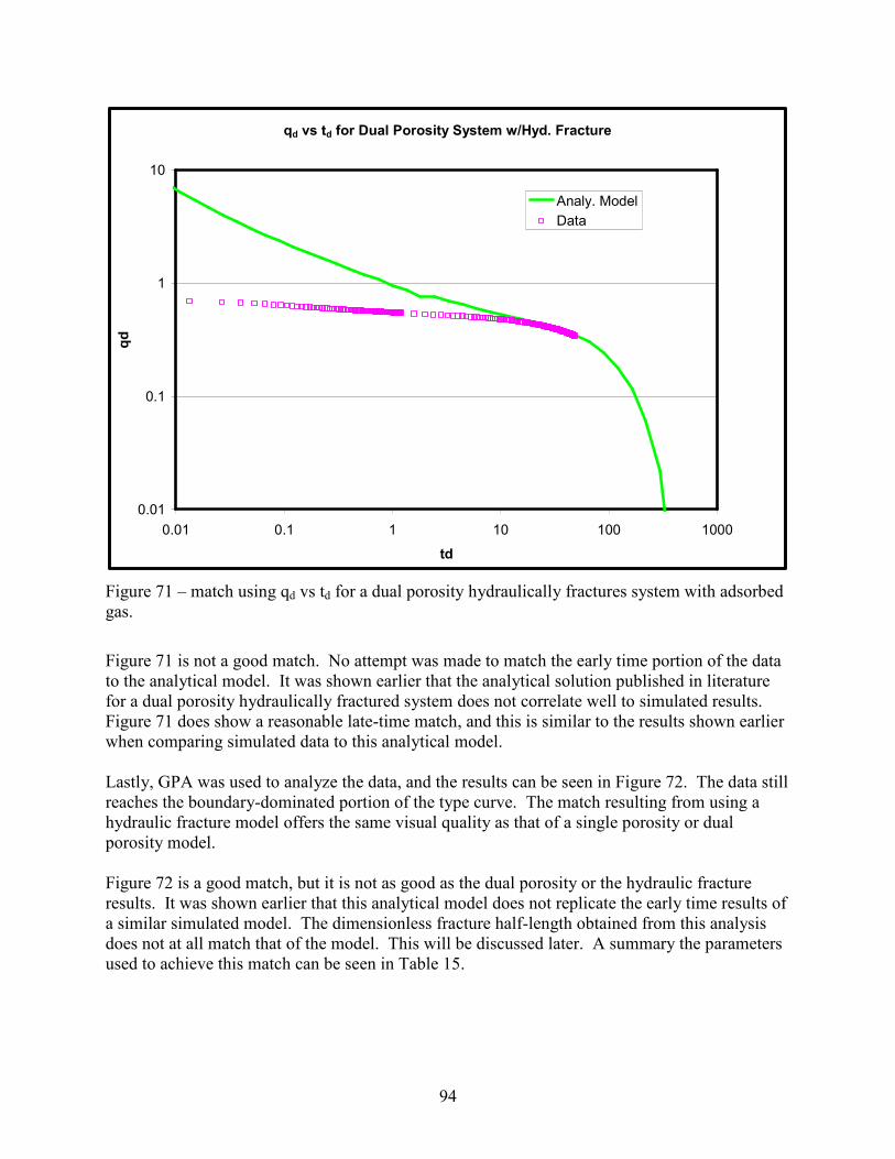
94
qd vs td for Dual Porosity System w/Hyd. Fracture
0.01
0.1
1
10
0.01 0.1 1 10 100 1000
td
qd
Analy. Model
Data
Figure 71 – match using qd vs td for a dual porosity hydraulically fractures system with adsorbed
gas.
Figure 71 is not a good match. No attempt was made to match the early time portion of the data
to the analytical model. It was shown earlier that the analytical solution published in literature
for a dual porosity hydraulically fractured system does not correlate well to simulated results.
Figure 71 does show a reasonable late-time match, and this is similar to the results shown earlier
when comparing simulated data to this analytical model.
Lastly, GPA was used to analyze the data, and the results can be seen in Figure 72. The data still
reaches the boundary-dominated portion of the type curve. The match resulting from using a
hydraulic fracture model offers the same visual quality as that of a single porosity or dual
porosity model.
Figure 72 is a good match, but it is not as good as the dual porosity or the hydraulic fracture
results. It was shown earlier that this analytical model does not replicate the early time results of
a similar simulated model. The dimensionless fracture half-length obtained from this analysis
does not at all match that of the model. This will be discussed later. A summary the parameters
used to achieve this match can be seen in Table 15.
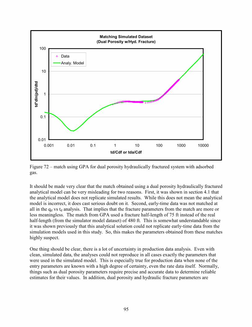
95
Matching Simulated Dataset
(Dual Porosity w/Hyd. Fracture)
0.01
0.1
1
10
100
0.001 0.01 0.1 1 10 100 1000 10000
td/Cdf or tda/Cdf
td*dln(pd)/dtd
Data
Analy. Model
Figure 72 – match using GPA for dual porosity hydraulically fractured system with adsorbed
gas.
It should be made very clear that the match obtained using a dual porosity hydraulically fractured
analytical model can be very misleading for two reasons. First, it was shown in section 4.1 that
the analytical model does not replicate simulated results. While this does not mean the analytical
model is incorrect, it does cast serious doubt on it. Second, early-time data was not matched at
all in the qd vs td analysis. That implies that the fracture parameters from the match are more or
less meaningless. The match from GPA used a fracture half-length of 75 ft instead of the real
half-length (from the simulator model dataset) of 480 ft. This is somewhat understandable since
it was shown previously that this analytical solution could not replicate early-time data from the
simulation models used in this study. So, this makes the parameters obtained from these matches
highly suspect.
One thing should be clear, there is a lot of uncertainty in production data analysis. Even with
clean, simulated data, the analyses could not reproduce in all cases exactly the parameters that
were used in the simulated model. This is especially true for production data when none of the
entry parameters are known with a high degree of certainty, even the rate data itself. Normally,
things such as dual porosity parameters require precise and accurate data to determine reliable
estimates for their values. In addition, dual porosity and hydraulic fracture parameters are

96
Table 15 – Summary of matching parameters for dual porosity hydraulically fractured systems
with adsorbed gas
Drainage
radius, re
(ft)
Porosity
( mφ )
Matrix
Perm.
(md)
xe/xf Cdf G/A* Match Term
( AkG φ ) *
qd vs td 3000 0.1 0.3 5.5 0.4 0.33 n/a
GPA
(pwd vs tda_new) 2640 0.05 1.1 35 0.6 0.32 3.52
Actual
(from model) 2640 0.1
1.8 (kf)
0.01 (km) 5.5 0.3 0.32 5.76**
obtained from early time data. This is when a well is just brought on production; the data is at its
least reliable at this time especially if the well is cleaning up. If one jumps at the opportunity to
use a more complicated model without any knowledge of the region, reservoir, or well
characteristics, substantial amounts of time may be used for little to no additional information
obtained. Also, assuming that this simulated dataset is representative of shale gas reservoir
performance suggests these reservoirs do not exhibit substantial effects of hydraulic fracturing.
They behave more like dual porosity reservoirs without hydraulic fractures.
Lastly, GPA can provide valuable insight were other analysis methodologies fail to provide any
definitive insight. In every case presented here, GPA has shown the production data reaches
boundary-dominated flow much earlier than the other analysis methods do. This is extremely
important for the both the accuracy and usefulness of the analysis performed. For example, it is
perfectly reasonable to assume a case where less than 10 years of production data is available.
This could mean that the production data reaches boundary-dominated flow on a GPA plot, but
does not reach it on a Fetkovich plot. On a cautionary note, GPA relies on a diagnostic plot (i.e.
derivative plot) to identify flow regimes and provide a good, sometimes better, match. However,
this approach may fail in the presence of very noisy production data. To some degree,
smoothing production can address this problem. It is also a fairly reasonable approach given that
the shape and length of the production rate and pressure curves are what are really important
when doing GPA. It is common practice when doing production data analysis to disregard entire
groups of data points that are considered unreliable or just simply wrong. In addition, data
smoothing is much less time consuming than re-initialization which is virtually always required
to perform a proper Fetkovich analysis.
6.2 Barnett Shale Example Well #1
Now, the insights gained from the simulation example cases detailed previously will be applied
to a field case. In particular, it was shown that adsorption does not have a large impact on the
analysis when vL is small and pL is large which is the case for this field case. It was also shown
that an analysis based on a complicated reservoir model does not always increase the amount of
information obtained from the analysis, but it does not hurt the analysis results (i.e. nothing is
lost).
6.2.1 Data and Data Handling
Production data for 32 months of what will be called Barnett Shale Example Well #1 were
obtained from a database provided by Devon Energy Corporation. Daily gas rate, oil rate, water
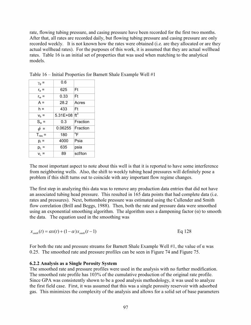
97
rate, flowing tubing pressure, and casing pressure have been recorded for the first two months.
After that, all rates are recorded daily, but flowing tubing pressure and casing pressure are only
recorded weekly. It is not known how the rates were obtained (i.e. are they allocated or are they
actual wellhead rates). For the purposes of this work, it is assumed that they are actual wellhead
rates. Table 16 is an initial set of properties that was used when matching to the analytical
models.
Table 16 – Initial Properties for Barnett Shale Example Well #1
γg = 0.6
re = 625 Ft
rw = 0.33 Ft
A = 28.2 Acres
h = 433 Ft
vb = 5.31E+08 ft3
Sw = 0.3 Fraction
φ = 0.06255 Fraction
Tres = 180 oF
pi = 4000 Psia
pL = 635 psia
vL = 89 scf/ton
The most important aspect to note about this well is that it is reported to have some interference
from neighboring wells. Also, the shift to weekly tubing head pressures will definitely pose a
problem if this shift turns out to coincide with any important flow regime changes.
The first step in analyzing this data was to remove any production data entries that did not have
an associated tubing head pressure. This resulted in 165 data points that had complete data (i.e.
rates and pressures). Next, bottomhole pressure was estimated using the Cullender and Smith
flow correlation (Brill and Beggs, 1988). Then, both the rate and pressure data were smoothed
using an exponential smoothing algorithm. The algorithm uses a dampening factor (α) to smooth
the data. The equation used in the smoothing was
)1()1()()( −−+= txtxtx smthsmth αα Eq 128
For both the rate and pressure streams for Barnett Shale Example Well #1, the value of α was
0.25. The smoothed rate and pressure profiles can be seen in Figure 74 and Figure 75.
6.2.2 Analysis as a Single Porosity System
The smoothed rate and pressure profiles were used in the analysis with no further modification.
The smoothed rate profile has 103% of the cumulative production of the original rate profile.
Since GPA was consistently shown to be a good analysis methodology, it was used to analyze
the first field case. First, it was assumed that this was a single porosity reservoir with adsorbed
gas. This minimizes the complexity of the analysis and allows for a solid set of base parameters

98
with which to do more complicated analysis. The correction for compressibility proposed by
Bumb and McKee (1988) was applied. To test the robustness of the match, 3 values of initial
pressure were used (4000 psi, 5000 psi, and 6000 psi). This parameter is perhaps the most
difficult parameter to obtain in a low permeability shale-gas system, and it is the most critical
parameter in the material balance time approach to production data analysis. In addition, the
values of the adsorption parameters will be increased in one trial to show the effect of using
different adsorption parameters. The individual match plots for each pressure are not shown
here, but the visual result was the same in all three cases and can be seen in Figure 76. The
match plots for the initial pressures of 5000 psi and 6000 psi can be seen in the Appendix A.
Data for Barnett Shale Example Well #1
0.1
1
10
100
1000
10000
0 200 400 600 800 1000 1200
Time (days)
Gas Rate, Water Rate, GLR
Gas Rate (MSCF/day)
Water Rate (STB/day)
GLR (MSCF/BBL)
FBHP (psia)
Figure 73 – Combined data plot for Barnett Shale Example Well #1
Figure 76 shows the match of Barnett Shale Example Well #1. The first thing that should be
noted is the lack of any early-time or radial flow match to the analytical solution. What could be
considered a radial flow section appears to be 2 to 3 times the typical value for radial flow of 0.5.
This seems to indicate that there are multiple (2 or 3) boundaries of some sort affecting this
system. In this case, both the dimensionless pressure and the dimensionless pressure derivative
were used to constrain the match. At late-time, both pwd and pwd’ overlay the type curve. If an
attempt is made to match the early-time portion of the data, it is not possible to get both pwd and
pwd’ to simultaneously overlay the type curve. This was evidence that the early-time data will
not fit a single porosity type curve. This could be because the data does not come from a single
porosity system or the data are inaccurate. A summary of the results for this match can be seen
in Table 17.
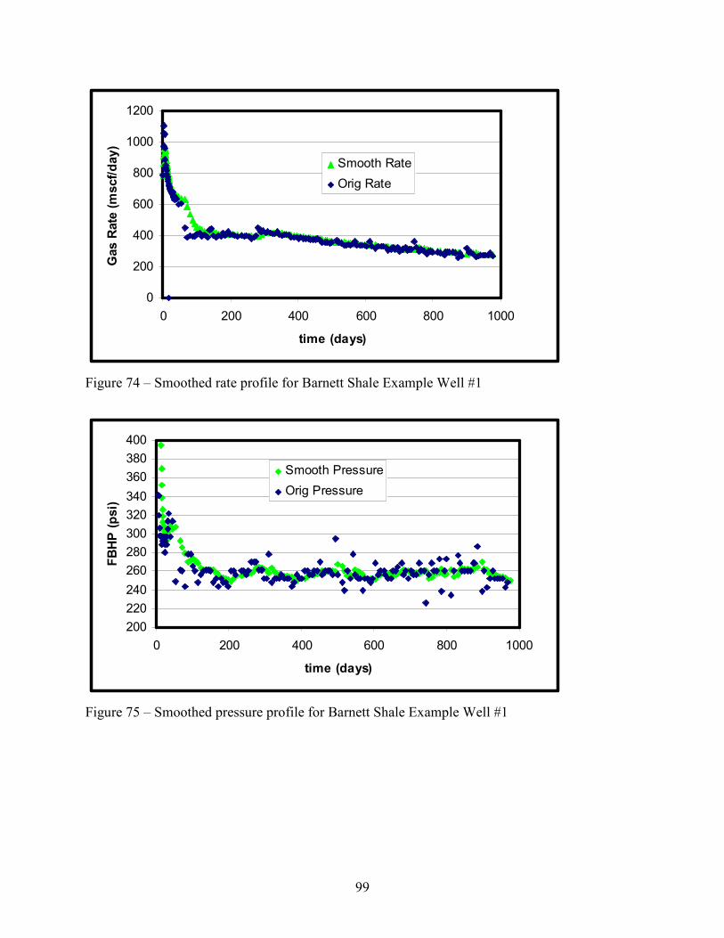
99
0
200
400
600
800
1000
1200
0 200 400 600 800 1000
time (days)
Gas Rate (mscf/day)
Smooth Rate
Orig Rate
Figure 74 – Smoothed rate profile for Barnett Shale Example Well #1
200
220
240
260
280
300
320
340
360
380
400
0 200 400 600 800 1000
time (days)
FBHP (psi)
Smooth Pressure
Orig Pressure
Figure 75 – Smoothed pressure profile for Barnett Shale Example Well #1

100
Matching Barnett Shale Example Well #1
(Single Porosity)
0.01
0.1
1
10
100
1000
10 100 1000 10000 100000 1000000 10000000 1E+08 1E+09
td or tda_new
pwd or pwd'
Data (Pwd) Data (Pwd')Analy. Model (300ft) Analy. Model (300ft)Analy. Model (500ft) Analy. Model (500ft)Analy. Model (1000ft) Analy. Model (1000ft)
Figure 76 – match using GPA for Barnett Shale Example Well #1 assumed to be a single
porosity system with initial pressure of 4000 psi.
6.2.3 Analysis as Dual Porosity System
Next, the data from this well was analyzed as a dual porosity system to see if any additional
information can be obtained. The correction for compressibility proposed by Bumb and McKee
(1988) was applied.
Figure 77 shows the match of Barnett Shale Example Well #1 assuming it is a dual porosity
system. In this case, both the dimensionless pressure and the dimensionless pressure derivative
were used to constrain the match. Figure 77 shows a better overall match to the entire dataset
rather than just late-time, especially for pwd’. There are what appear to be two flat portions on the derivative curve of the analytic model. These flat portions are separated by sections of unit-
slope. These flat portions can be interpreted as two distinct radial flow periods separated by
boundary dominated flow. The first representing radial flow through a fracture system, and the
second representing radial flow through the matrix. The first section of boundary dominated
flow occurs when the boundary is seen through the fracture system. The second section occurs
when a boundary is seen through the matrix. While the second radial-flow portion of this dataset
does not perfectly overlay the type curve, the trend is clearly seen. An alternative interpretation
is that this data comes from a multilayered reservoir. However, information to substantiate this
interpretation was not provided. A summary of the results from this match can be seen in Table
17.
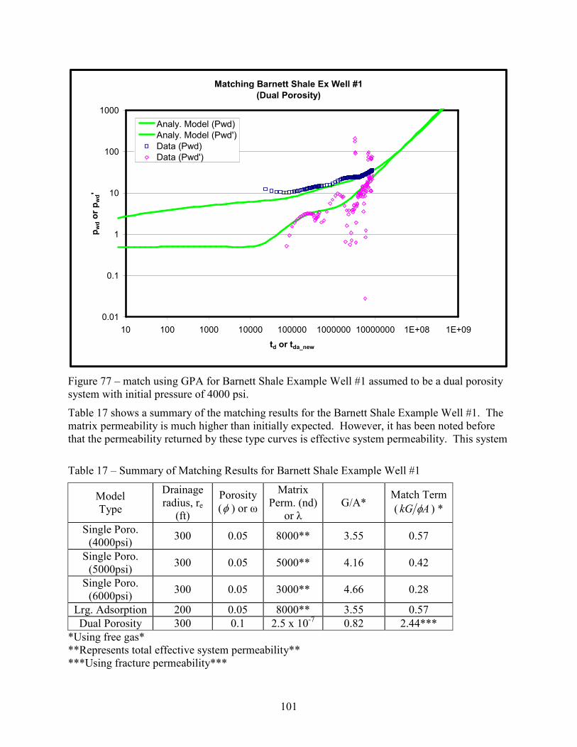
101
Matching Barnett Shale Ex Well #1
(Dual Porosity)
0.01
0.1
1
10
100
1000
10 100 1000 10000 100000 1000000 10000000 1E+08 1E+09
td or tda_new
pwd or pwd'
Analy. Model (Pwd)
Analy. Model (Pwd')
Data (Pwd)
Data (Pwd')
Figure 77 – match using GPA for Barnett Shale Example Well #1 assumed to be a dual porosity
system with initial pressure of 4000 psi.
Table 17 shows a summary of the matching results for the Barnett Shale Example Well #1. The
matrix permeability is much higher than initially expected. However, it has been noted before
that the permeability returned by these type curves is effective system permeability. This system
Table 17 – Summary of Matching Results for Barnett Shale Example Well #1
Model
Type
Drainage
radius, re
(ft)
Porosity
(φ ) or ω
Matrix
Perm. (nd)
or λ
G/A* Match Term
( AkG φ ) *
Single Poro.
(4000psi) 300 0.05 8000** 3.55 0.57
Single Poro.
(5000psi) 300 0.05 5000** 4.16 0.42
Single Poro.
(6000psi) 300 0.05 3000** 4.66 0.28
Lrg. Adsorption 200 0.05 8000** 3.55 0.57
Dual Porosity 300 0.1 2.5 x 10⁻⁷ 0.82 2.44***
*Using free gas*
**Represents total effective system permeability**
***Using fracture permeability***

102
is most likely a dual porosity system, and the well is hydraulically fractured. Therefore, it is
reasonable to assume that it would behave as if it had a larger effective system permeability. The
drainage radius obtained is smaller than the initial dataset indicated. This could be due to the
interference that is known to affect the performance of this well. It could also be reality. A
reasonable scenario in this situation is for the drainage area to represent the stimulated region.
Shale gas reservoirs have very low permeability; it is not unreasonable to assume that little or no
production or pressure support is coming from areas not directly connected to the hydraulic
fracture system. This is somewhat supported by the fact that the analysis indicates that the
average reservoir pressure has dropped from 4000 psi down to 2200 psi.
Changing the adsorption parameters does have an effect on the results of the analysis because the
correction for adsorption put forth by Bumb and McKee (1988) was used. However, to obtain a
noticeable shift in the position of the data on the type curve plot that could not be confused for
natural data scatter, a value for vL that was 8 times larger than the original value assumed was
required. As can be seen in Table 17, the effect is to have a larger match term ( AkG φ ). This is
attributed to the smaller drainage area that is required to match the data since a larger value for
vL shifts the data to the left on the type curve plot. Recall that adsorption effects system
compressibility in this type of analysis. With a larger system compressibility due to adsorption,
this causes tda_new to be smaller at any given point (recall the definition of tda_new in Eq 124). This
requires using either a smaller drainage radius in the analytical solution or a smaller porosity in
the calculation of the dimensionless plotting functions for the production data. A schematic of
this can be seen in Figure 78.
The varying of initial pressure does not have a large effect on the outcome of the matching
process. While the match term does decrease in value, a change in initial pressure does not truly
affect tda_new because any increase in initial pressure is offset by an increase in gas in place.
Thus, an increase in the initial pressure results in a positive vertical shift of the data on the type
curve plot because it effects dimensionless pressure, not tda_new. This vertical shift is best
counteracted by decreasing the permeability or the reservoir thickness. This is reflected in the
changes to the match term AkG φ . Permeability is in tda_new, so there will be a slight horizontal
shift in the end. It is conceivable that a very large change in initial pressure could cause a
significant increase in estimated permeability that would have to be offset by changing other
match parameters. But, that was not the case here. However, do not underestimate the
importance of knowing initial pressure accurately. Any uncertainty in this parameter effects
every parameter returned from the analysis.
An important thing to note about the data from Table 17 is the true nature of the matching/output
parameters obtained from production data analysis. For example, the match for the dual porosity
system will return a value of λ, ω, and dimensionless radius (rd) used to generate the analytical
type curve. The production data will return a value for the match term ( AkG φ ). If the value of
any specific parameter is desired, an assumption will have to be made. If one wants fracture
permeability from λ, values for matrix permeability, wellbore radius, fracture spacing, and
fracture geometry must be provided. These values can in no way be determined from the match
without additional information and/or assumptions.
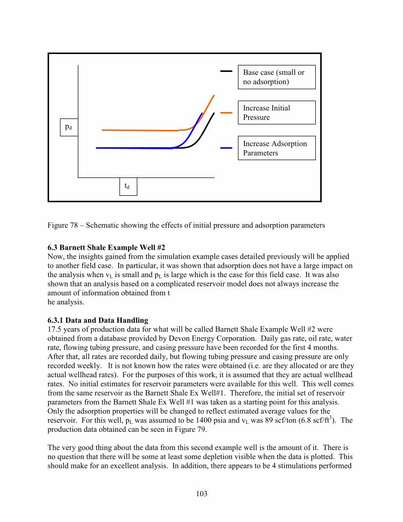
103
Figure 78 – Schematic showing the effects of initial pressure and adsorption parameters
6.3 Barnett Shale Example Well #2
Now, the insights gained from the simulation example cases detailed previously will be applied
to another field case. In particular, it was shown that adsorption does not have a large impact on
the analysis when vL is small and pL is large which is the case for this field case. It was also
shown that an analysis based on a complicated reservoir model does not always increase the
amount of information obtained from t
he analysis.
6.3.1 Data and Data Handling
17.5 years of production data for what will be called Barnett Shale Example Well #2 were
obtained from a database provided by Devon Energy Corporation. Daily gas rate, oil rate, water
rate, flowing tubing pressure, and casing pressure have been recorded for the first 4 months.
After that, all rates are recorded daily, but flowing tubing pressure and casing pressure are only
recorded weekly. It is not known how the rates were obtained (i.e. are they allocated or are they
actual wellhead rates). For the purposes of this work, it is assumed that they are actual wellhead
rates. No initial estimates for reservoir parameters were available for this well. This well comes
from the same reservoir as the Barnett Shale Ex Well#1. Therefore, the initial set of reservoir
parameters from the Barnett Shale Ex Well #1 was taken as a starting point for this analysis.
Only the adsorption properties will be changed to reflect estimated average values for the
reservoir. For this well, pL was assumed to be 1400 psia and vL was 89 scf/ton (6.8 scf/ft3). The
production data obtained can be seen in Figure 79.
The very good thing about the data from this second example well is the amount of it. There is
no question that there will be some at least some depletion visible when the data is plotted. This
should make for an excellent analysis. In addition, there appears to be 4 stimulations performed
td
pd
Base case (small or
no adsorption)
Increase Initial
Pressure
Increase Adsorption
Parameters
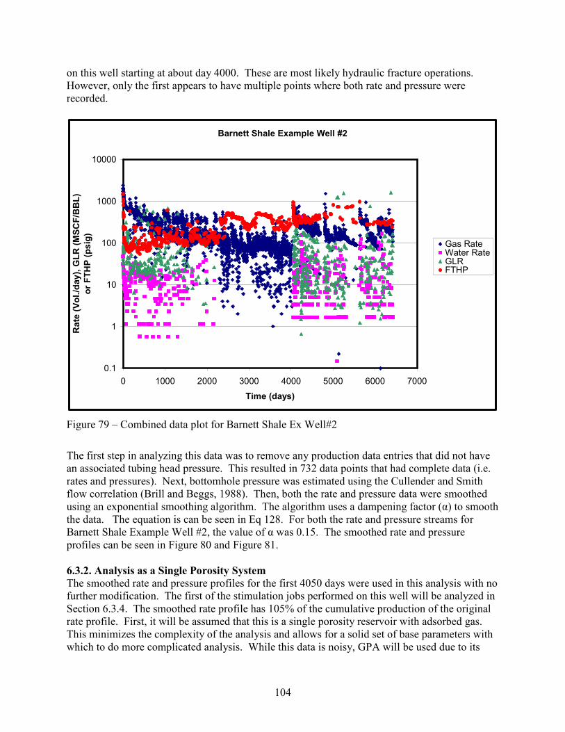
104
on this well starting at about day 4000. These are most likely hydraulic fracture operations.
However, only the first appears to have multiple points where both rate and pressure were
recorded.
Barnett Shale Example Well #2
0.1
1
10
100
1000
10000
0 1000 2000 3000 4000 5000 6000 7000
Time (days)
Rate (Vol./day), GLR (MSCF/BBL)
or FTHP (psig)
Gas RateWater RateGLRFTHP
Figure 79 – Combined data plot for Barnett Shale Ex Well#2
The first step in analyzing this data was to remove any production data entries that did not have
an associated tubing head pressure. This resulted in 732 data points that had complete data (i.e.
rates and pressures). Next, bottomhole pressure was estimated using the Cullender and Smith
flow correlation (Brill and Beggs, 1988). Then, both the rate and pressure data were smoothed
using an exponential smoothing algorithm. The algorithm uses a dampening factor (α) to smooth
the data. The equation is can be seen in Eq 128. For both the rate and pressure streams for
Barnett Shale Example Well #2, the value of α was 0.15. The smoothed rate and pressure
profiles can be seen in Figure 80 and Figure 81.
6.3.2. Analysis as a Single Porosity System
The smoothed rate and pressure profiles for the first 4050 days were used in this analysis with no
further modification. The first of the stimulation jobs performed on this well will be analyzed in
Section 6.3.4. The smoothed rate profile has 105% of the cumulative production of the original
rate profile. First, it will be assumed that this is a single porosity reservoir with adsorbed gas.
This minimizes the complexity of the analysis and allows for a solid set of base parameters with
which to do more complicated analysis. While this data is noisy, GPA will be used due to its
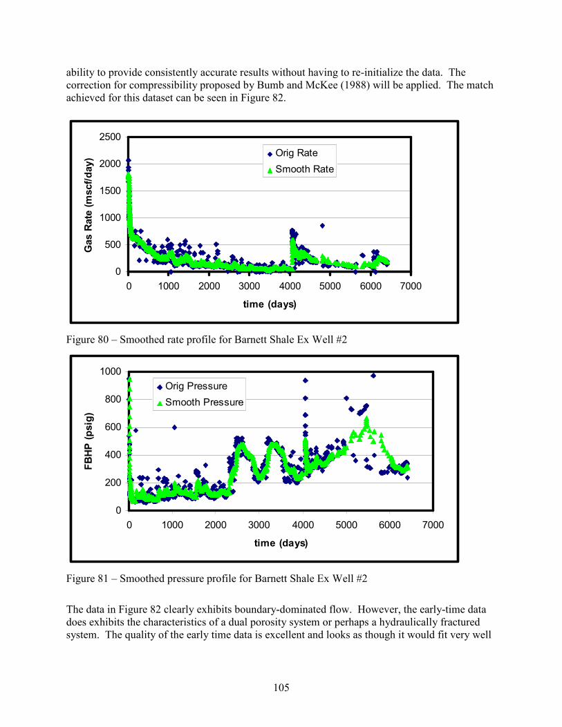
105
ability to provide consistently accurate results without having to re-initialize the data. The
correction for compressibility proposed by Bumb and McKee (1988) will be applied. The match
achieved for this dataset can be seen in Figure 82.
0
500
1000
1500
2000
2500
0 1000 2000 3000 4000 5000 6000 7000
time (days)
Gas Rate (mscf/day)
Orig Rate
Smooth Rate
Figure 80 – Smoothed rate profile for Barnett Shale Ex Well #2
0
200
400
600
800
1000
0 1000 2000 3000 4000 5000 6000 7000
time (days)
FBHP (psig)
Orig Pressure
Smooth Pressure
Figure 81 – Smoothed pressure profile for Barnett Shale Ex Well #2
The data in Figure 82 clearly exhibits boundary-dominated flow. However, the early-time data
does exhibits the characteristics of a dual porosity system or perhaps a hydraulically fractured
system. The quality of the early time data is excellent and looks as though it would fit very well
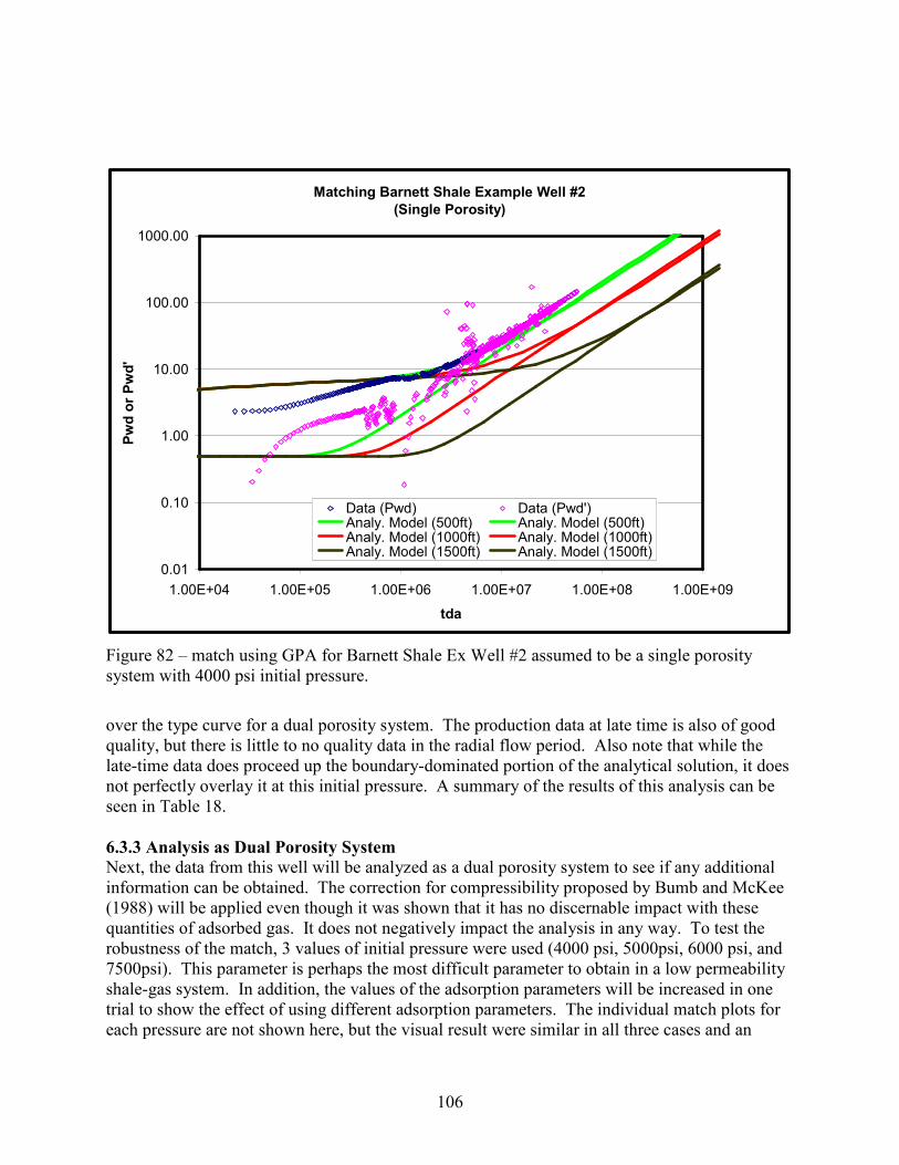
106
Matching Barnett Shale Example Well #2
(Single Porosity)
0.01
0.10
1.00
10.00
100.00
1000.00
1.00E+04 1.00E+05 1.00E+06 1.00E+07 1.00E+08 1.00E+09
tda
Pwd or Pwd'
Data (Pwd) Data (Pwd')Analy. Model (500ft) Analy. Model (500ft)Analy. Model (1000ft) Analy. Model (1000ft)Analy. Model (1500ft) Analy. Model (1500ft)
Figure 82 – match using GPA for Barnett Shale Ex Well #2 assumed to be a single porosity
system with 4000 psi initial pressure.
over the type curve for a dual porosity system. The production data at late time is also of good
quality, but there is little to no quality data in the radial flow period. Also note that while the
late-time data does proceed up the boundary-dominated portion of the analytical solution, it does
not perfectly overlay it at this initial pressure. A summary of the results of this analysis can be
seen in Table 18.
6.3.3 Analysis as Dual Porosity System
Next, the data from this well will be analyzed as a dual porosity system to see if any additional
information can be obtained. The correction for compressibility proposed by Bumb and McKee
(1988) will be applied even though it was shown that it has no discernable impact with these
quantities of adsorbed gas. It does not negatively impact the analysis in any way. To test the
robustness of the match, 3 values of initial pressure were used (4000 psi, 5000psi, 6000 psi, and
7500psi). This parameter is perhaps the most difficult parameter to obtain in a low permeability
shale-gas system. In addition, the values of the adsorption parameters will be increased in one
trial to show the effect of using different adsorption parameters. The individual match plots for
each pressure are not shown here, but the visual result were similar in all three cases and an
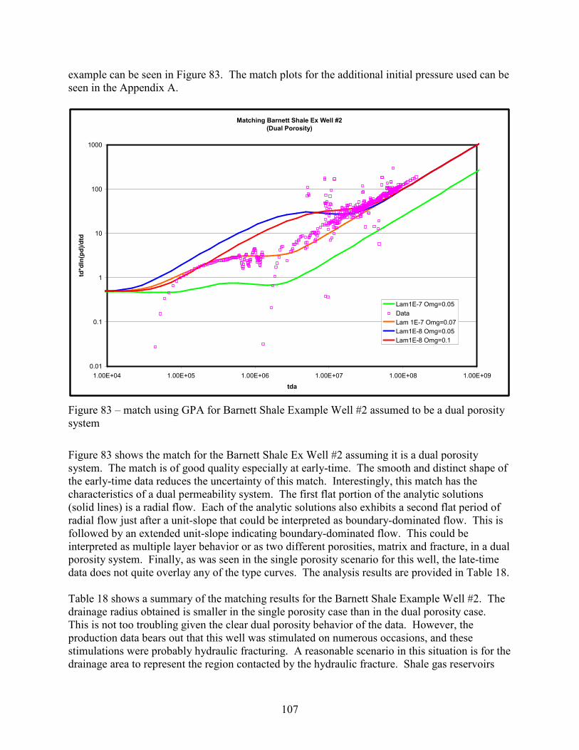
107
example can be seen in Figure 83. The match plots for the additional initial pressure used can be
seen in the Appendix A.
Matching Barnett Shale Ex Well #2
(Dual Porosity)
0.01
0.1
1
10
100
1000
1.00E+04 1.00E+05 1.00E+06 1.00E+07 1.00E+08 1.00E+09
tda
td*dln(pd)/dtd
Lam1E-7 Omg=0.05
Data
Lam 1E-7 Omg=0.07
Lam1E-8 Omg=0.05
Lam1E-8 Omg=0.1
Figure 83 – match using GPA for Barnett Shale Example Well #2 assumed to be a dual porosity
system
Figure 83 shows the match for the Barnett Shale Ex Well #2 assuming it is a dual porosity
system. The match is of good quality especially at early-time. The smooth and distinct shape of
the early-time data reduces the uncertainty of this match. Interestingly, this match has the
characteristics of a dual permeability system. The first flat portion of the analytic solutions
(solid lines) is a radial flow. Each of the analytic solutions also exhibits a second flat period of
radial flow just after a unit-slope that could be interpreted as boundary-dominated flow. This is
followed by an extended unit-slope indicating boundary-dominated flow. This could be
interpreted as multiple layer behavior or as two different porosities, matrix and fracture, in a dual
porosity system. Finally, as was seen in the single porosity scenario for this well, the late-time
data does not quite overlay any of the type curves. The analysis results are provided in Table 18.
Table 18 shows a summary of the matching results for the Barnett Shale Example Well #2. The
drainage radius obtained is smaller in the single porosity case than in the dual porosity case.
This is not too troubling given the clear dual porosity behavior of the data. However, the
production data bears out that this well was stimulated on numerous occasions, and these
stimulations were probably hydraulic fracturing. A reasonable scenario in this situation is for the
drainage area to represent the region contacted by the hydraulic fracture. Shale gas reservoirs

108
have very low permeability; it is not unreasonable to assume that no little or no production or
pressure support is coming from areas not directly connected to the hydraulic fracture system.
This very small drainage radius might very well be an effective drainage volume which is
connected by the hydraulic fractures. This theory will be put to the test in Section 6.3.4.
Table 18 – Summary of matching results for Barnett Shale Ex Well #2
Model
Type
Drainage
radius, re
(ft)
Porosity
( mφ ) or
ω
Matrix
Perm. (nd)
or λ G/A*
Match
Term
( AkG φ ) *
Single Porosity 350 0.0175 7000** 1.63 0.65
Dual Poro.
(4000 psi) 500 0.085 1 x 10
-7 1.12 1.12
Dual Poro.
(5000psi) 500 0.085 1 x 10
-7 1.07 1.0
Dual Poro.
(6000psi) 500 0.085 1 x 10
-7 0.99 0.98
Dual Poro.
(7500psi) 500 0.095 1 x 10
-7 0.36 0.95
Lrg. Adsorption 350 0.07 1 x 10⁻⁷ 0.97 3.28***
*Using free gas. G/A with adsorbed gas is 2.65 for 7500 psi, 2.98 for 5000 psi, and 3.11 for
4000 psi.*
**Represents total effective system permeability**
***Using fracture permeability***
The exercise to determine the sensitivity of the match to initial pressure was performed on the
dual porosity cases because the data exhibits dual porosity behavior. The dual porosity
parameters (λ and ω) did not initially change with pressure because initial pressure did not affect
the shape of the data curve; it only affected its position on the type curve plot. The shape is what
determines λ and ω. As initial pressure was increased, matrix porosity was decreased in an
attempt to match the late-time portion of the analytic type curve. Fracture porosity was also
changed to preserve the same value of ω. However, for the case of 7500 psi initial pressure,
matrix porosity became small enough that a slightly larger ω was thought to be a better match.
The match for 5000 psi and 6000 psi can be seen in the Appendix A.
Figure 84 is the match for Barnett Shale Ex Well #2 at 7500 psi. When performing log-log
production data analysis, it is very important to achieve a very good match at late-time. It was
necessary to increase the initial pressure to 7500 psi which is a higher pressure than expected for
this field. This allowed a smaller porosity to be used without material balance indicating an
unreasonably low reservoir pressure at the end of this production period. The reservoir pressure
at the end of this production period was estimated to be about 600 psi. Flowing bottomhole
pressures at the end of this production period are about 250 psi and gas production rates are
about 100 MSCF/day.
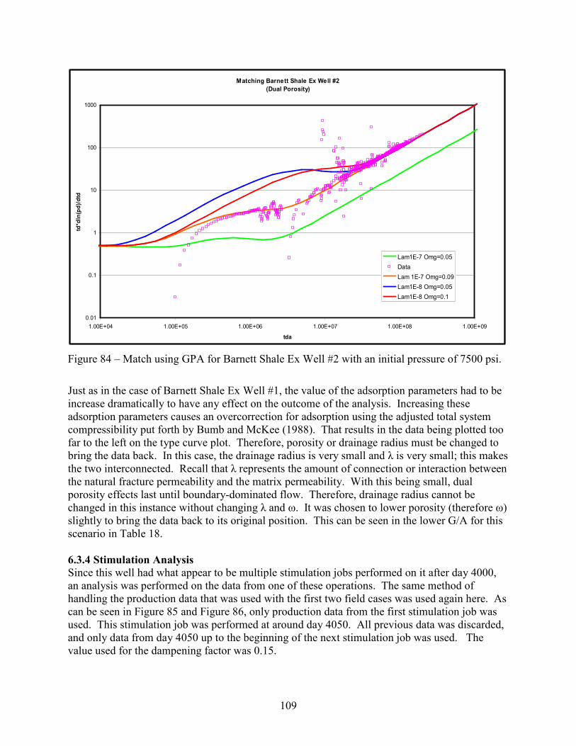
109
Matching Barnett Shale Ex Well #2
(Dual Porosity)
0.01
0.1
1
10
100
1000
1.00E+04 1.00E+05 1.00E+06 1.00E+07 1.00E+08 1.00E+09
tda
td*dln(pd)/dtd
Lam1E-7 Omg=0.05
Data
Lam 1E-7 Omg=0.09
Lam1E-8 Omg=0.05
Lam1E-8 Omg=0.1
Figure 84 – Match using GPA for Barnett Shale Ex Well #2 with an initial pressure of 7500 psi.
Just as in the case of Barnett Shale Ex Well #1, the value of the adsorption parameters had to be
increase dramatically to have any effect on the outcome of the analysis. Increasing these
adsorption parameters causes an overcorrection for adsorption using the adjusted total system
compressibility put forth by Bumb and McKee (1988). That results in the data being plotted too
far to the left on the type curve plot. Therefore, porosity or drainage radius must be changed to
bring the data back. In this case, the drainage radius is very small and λ is very small; this makes
the two interconnected. Recall that λ represents the amount of connection or interaction between
the natural fracture permeability and the matrix permeability. With this being small, dual
porosity effects last until boundary-dominated flow. Therefore, drainage radius cannot be
changed in this instance without changing λ and ω. It was chosen to lower porosity (therefore ω)
slightly to bring the data back to its original position. This can be seen in the lower G/A for this
scenario in Table 18.
6.3.4 Stimulation Analysis
Since this well had what appear to be multiple stimulation jobs performed on it after day 4000,
an analysis was performed on the data from one of these operations. The same method of
handling the production data that was used with the first two field cases was used again here. As
can be seen in Figure 85 and Figure 86, only production data from the first stimulation job was
used. This stimulation job was performed at around day 4050. All previous data was discarded,
and only data from day 4050 up to the beginning of the next stimulation job was used. The
value used for the dampening factor was 0.15.
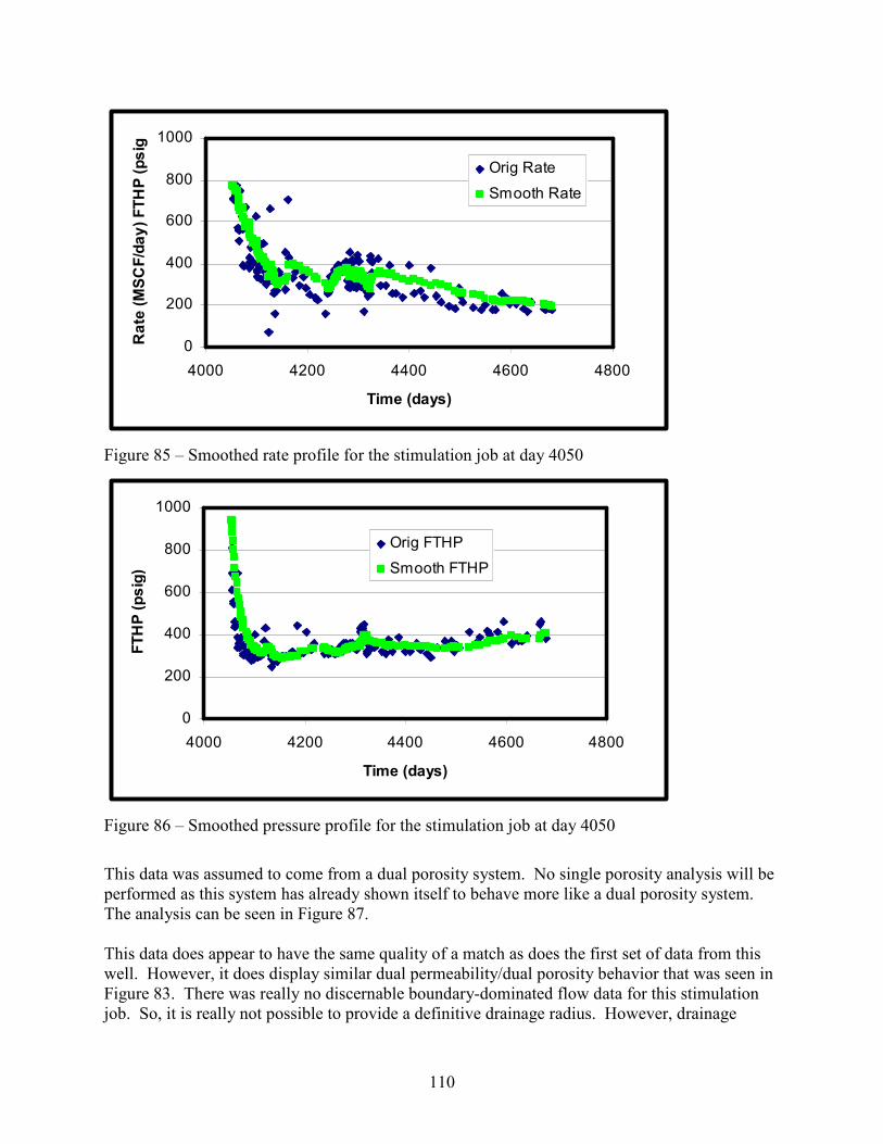
110
0
200
400
600
800
1000
4000 4200 4400 4600 4800
Time (days)
Rate (MSCF/day) FTHP (psig)
Orig Rate
Smooth Rate
Figure 85 – Smoothed rate profile for the stimulation job at day 4050
0
200
400
600
800
1000
4000 4200 4400 4600 4800
Time (days)
FTHP (psig)
Orig FTHP
Smooth FTHP
Figure 86 – Smoothed pressure profile for the stimulation job at day 4050
This data was assumed to come from a dual porosity system. No single porosity analysis will be
performed as this system has already shown itself to behave more like a dual porosity system.
The analysis can be seen in Figure 87.
This data does appear to have the same quality of a match as does the first set of data from this
well. However, it does display similar dual permeability/dual porosity behavior that was seen in
Figure 83. There was really no discernable boundary-dominated flow data for this stimulation
job. So, it is really not possible to provide a definitive drainage radius. However, drainage

111
radius does slightly impact λ and ω if λ is small enough to cause dual-porosity effects to last until
late-time. Therefore, this match is somewhat indicative of drainage radius. The dimensionless
radius obtained from this match is less than what was obtained previously for this well. A
summary of the results can be seen in Table 19.
Matching Barnett Shale Ex Well#2 (Stimulation)
(Dual Porosity)
0.1
1
10
100
1000
100 1000 10000 100000 1000000 10000000 100000000
td or tda_new
pwd'
Analytical Model
Data
Figure 87 – match using GPA for the first stimulation job performed on Barnett Shale Ex Well
#2
This match was achieved with the roughly the same dual porosity parameters and the same initial
pressure as was used on the first section of data from this well. The small drainage radius is the
most notable difference between the results of this match and the previous match. However, if
one assumes that this well was hydraulically fractured before and then re-fractured at day 4050,
this can make sense. Let us assume that the only producing portions of the reservoir are those
Table 19 – Summary of matching results for the first stimulation job performed on Barnett Shale
Ex Well #2
Model
Type
Drainage
radius, re
(ft)
ω Λ G/A*
Match
Term
( AkG φ ) *
Dual Porosity 225 0.075 9E-8 3.52 2.49

112
directly connected to the hydraulic fracture by the natural fracture matrix. This assumption is
reasonable if one also assumes that any hydraulic fracture in the shale reservoir merely props
open the natural fracture matrix (Gale, et al. 2007). This area that is connected to the hydraulic
fracture is very small and is drained rapidly. This is evident when matching the first data section
of this well; the average reservoir pressure estimated at for the last data point was 700 psi. This
is more than a 3000 psi drop in reservoir pressure from the initial reservoir pressure of 4000 psi.
As production declines, it becomes necessary to contact new reservoir. Another fracture
operation is performed and the well resumes producing at its original high rate. According to the
analysis here, reservoir pressures seen after the fracturing are at or near original reservoir
pressure. Each time the well is fractured additional, apparently new reservoir area is contacted.
This can be seen by comparing the initial rates of the all of the stimulation jobs that can be seen
in Figure 79 and the fact that both the first data section on the stimulated data section can be
matched using the same initial pressure and the same dual porosity parameters.

113
7. SUMMARY, CONCLUSIONS, AND RECOMMENDATIONS
7.1 Summary
It was shown from the beginning of this work that there was a gap in the understanding of how
adsorption affects the analysis of production data. With the exception of a work by Bumb and
McKee (1988) that was expanded upon by Spivey and Semmelbeck (1996), all efforts pertaining
to understanding this phenomenon were focused on empirical relationships like those proposed
by Lane, et al. (1989).
This work has shown that production data from reservoirs that contain adsorbed gas can be
analyzed in dimensionless space. Using a combination of a semi-analytic time function (a
slightly modified version of material balance time from Palacio and Blasingame (1993)) and
analytical constant-rate solutions, production data from many of the common reservoir systems
are capable of being accurately analyzed regardless of whether or not they contain adsorbed gas.
This work has documented the effects of adsorption on four common reservoir systems: single
porosity, dual porosity, finite conductivity vertical fracture, and dual porosity with a finite
conductivity vertical fracture. Furthermore, it has been shown that a consistent analysis method
can be applied to these various systems to obtain an accurate analysis of production data from
reservoirs that contain adsorbed gas.
Also, three common analysis methods were examined to determine which, if any, yields superior
results in analyzing a simulated production dataset. The results from these various analysis
methods were compared against one another. Lastly, the insights gained from this work were
applied to two field datasets from the Barnett Shale provided by Devon Energy Corporation.
7.2 Conclusions
Agarwal (1999) confirmed that material balance time (Palacio and Blasingame, 1993) could be
used to convert a constant-pressure system to an equivalent constant-rate system. This was
reconfirmed in this work, and it was shown to work for the four types of reservoir systems shown
in this work. This was completely expected and very necessary since the application of GPA
(Cox, et al., 2002) depends on applying this methodology. In addition, the analytical solutions to
three of these four reservoir systems were shown to be identical to simulated results. The dual
porosity system with a finite conductivity vertical fracture was the only system in which the
simulated results did not match the analytical solution. This is most likely due to an inaccurate
analytical solution as only one example of a closed form solution for this type of system could be
found in the literature.
While adsorption is a complicated mechanism, its effects on production data and production data
analysis seem to be consistent and relatively simple. For systems produced at constant rate or
constant pressure, adsorbed gas causes a given rate or flowing bottom-hole pressure to be
sustained for a longer period of time compared to a system without adsorbed gas.
Mechanistically, this is logical in that adsorption acts to replenish free gas in the pore spaces that
has been produced as reservoir pressure is lowered. This effect can be, and usually is, greater at
late-time depending on the shape of the Langmuir isotherm.

114
In dimensionless space, adsorption is seen as an increase in system compressibility. This can be
calculated for any type of system using the equation provided by Bumb and McKee (1988).
Production data plotted without using this equation for compressibility in calculating the plotting
functions will plot too far to the right on the graph. This could result in several analysis errors,
but the most common would be a porosity that is too large or a dimensionless radius that is too
large. However, the effect of adsorption on dimensionless type curves can be very subtle
depending on the amount of adsorbed gas in relation to the amount of free gas. In many cases,
the effects of adsorption will not be noticeable, or it would be permissible to discount them given
the normal scatter and uncertainty that surrounds production data. It is foreseeable that coalbed
methane systems may have enough adsorbed gas relative to free gas that the effects of adsorption
would be noticeable and significant.
When using material balance time to convert a constant-pressure system to an equivalent
constant-rate system, two extra cautions must be taken. The use of material balance time makes
for a more complicated plotting function. Since it includes original gas in place, adsorption can
greatly affect where production falls on a dimensionless plot that uses material balance time to
calculate dimensionless time. Recall that none of the analytical solutions used in this work
account for adsorbed gas. It was shown that it is necessary to use free gas in the equation for
material balance time so that production data from a system with adsorbed gas will overlay an
analytical solution for the same system without adsorbed gas.
Secondly, the use of material balance time in dimensionless time eliminates compressibility from
the equation for the plotting function. Therefore, it was necessary to slightly modify the
equation for material balance time to allow compressibility to remain in the plotting function. It
is recommended to use this definition of material balance time when analyzing systems with
significant amounts of adsorbed gas.
Three common methods of analyzing production data analysis were compared using a simulated
dataset. In this particular case, GPA seemed to be the more effective method consistently
generating slightly more accurate results. More importantly, its use of a diagnostic (derivative)
curve enabled it to recognize late-time boundary dominated flow earlier than the other methods.
However, as with all material balance time methods its plotting functions require more inputs as
compared to the other analysis methods. Most importantly, they hinge on an accurate estimate of
initial pressure which is very hard to obtain in low permeability systems such as shale gas
reservoirs.
The analysis of the two field datasets yields two very important pieces of information. First, it
showed exactly what type of data can be returned from such an analysis. For the case of GPA,
an analyst can provide the values for the parameters that were used to calculate the matched
analytical model and a value for the term AkG φ . To obtain additional information, the value of
some other parameter must be assumed. But, the analysis has constrained the value of 4 very
important parameters.
In addition, it showed that GPA could be a valuable diagnostic tool for shale gas reservoirs. If
the analysis of the Barnett Shale Ex Well #2 is reasonably correct, analyzing the data from any
new fracture job performed on a well and comparing it to the original analysis will allow an
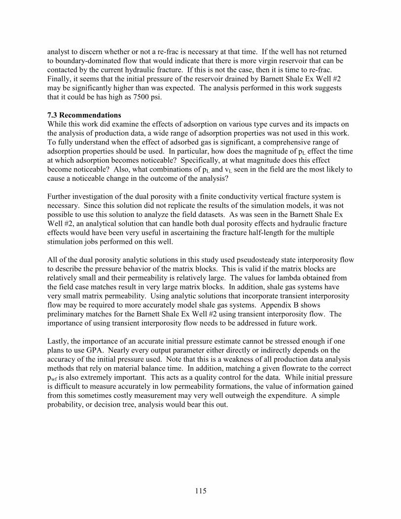
115
analyst to discern whether or not a re-frac is necessary at that time. If the well has not returned
to boundary-dominated flow that would indicate that there is more virgin reservoir that can be
contacted by the current hydraulic fracture. If this is not the case, then it is time to re-frac.
Finally, it seems that the initial pressure of the reservoir drained by Barnett Shale Ex Well #2
may be significantly higher than was expected. The analysis performed in this work suggests
that it could be has high as 7500 psi.
7.3 Recommendations While this work did examine the effects of adsorption on various type curves and its impacts on
the analysis of production data, a wide range of adsorption properties was not used in this work.
To fully understand when the effect of adsorbed gas is significant, a comprehensive range of
adsorption properties should be used. In particular, how does the magnitude of pL effect the time
at which adsorption becomes noticeable? Specifically, at what magnitude does this effect
become noticeable? Also, what combinations of pL and vL seen in the field are the most likely to
cause a noticeable change in the outcome of the analysis?
Further investigation of the dual porosity with a finite conductivity vertical fracture system is
necessary. Since this solution did not replicate the results of the simulation models, it was not
possible to use this solution to analyze the field datasets. As was seen in the Barnett Shale Ex
Well #2, an analytical solution that can handle both dual porosity effects and hydraulic fracture
effects would have been very useful in ascertaining the fracture half-length for the multiple
stimulation jobs performed on this well.
All of the dual porosity analytic solutions in this study used pseudosteady state interporosity flow
to describe the pressure behavior of the matrix blocks. This is valid if the matrix blocks are
relatively small and their permeability is relatively large. The values for lambda obtained from
the field case matches result in very large matrix blocks. In addition, shale gas systems have
very small matrix permeability. Using analytic solutions that incorporate transient interporosity
flow may be required to more accurately model shale gas systems. Appendix B shows
preliminary matches for the Barnett Shale Ex Well #2 using transient interporosity flow. The
importance of using transient interporosity flow needs to be addressed in future work.
Lastly, the importance of an accurate initial pressure estimate cannot be stressed enough if one
plans to use GPA. Nearly every output parameter either directly or indirectly depends on the
accuracy of the initial pressure used. Note that this is a weakness of all production data analysis
methods that rely on material balance time. In addition, matching a given flowrate to the correct
pwf is also extremely important. This acts as a quality control for the data. While initial pressure
is difficult to measure accurately in low permeability formations, the value of information gained
from this sometimes costly measurement may very well outweigh the expenditure. A simple
probability, or decision tree, analysis would bear this out.

116
REFERENCES
Agarwal, Ram G., David C. Gardner, Stanley W. Kleinsteiber, and Del. D Fussell: “Analyzing
Well Production Data Using Combined-Type-Curve and Decline-Curve Analysis Concepts,”
SPE 57916 presented at the SPE Annual Technical Conference and Exhibition, New Orleans,
September 27-30, 1999.
Aguilera, R.: “Well Test Analysis of Dual-Porosity Systems Intercpeted by Hydraulic Vertical
Fractures of Finite Conductivity,” SPE 18948 presented at the SPE Rocky Mountain
Regional/Low-Permeability Reservoirs Symposium, Denver, March 6-8, 1989.
Arps, J. J.: “Analysis of Decline Curves,” Published in Petroleum Transactions, AIME, 160
(1945): 228-247.
Blasingame, T. A. and W. J. Lee: “The Variable-Rate Reservoir Limits Testing of Gas Wells,”
SPE 17708 presented at the SPE Gas Technology Symposium, Dallas, June 13-15, 1988.
Brill, James P. and H. Dale Beggs: Two-Phase Flow in Pipes, 6th Ed, (1988).
Bumb, A. C. and C. R. McKee: “Gas Well Testing in the Presence of Desorption for Coalbed
Methane and Devonian Shale,” SPE Formation Evaluation, Vol. 3, No. 1 (1988, March): 179-
185.
Carter, Robert D.: “Characteristic Behavior of Finite Radial and Linear Gas Flow Systems-
Constant Terminal Pressure Case,” SPE/DOE 09887 presented at the SPE/DOE Low
Permeability Symposium, Denver, May 27-29, 1981.
Cinco-Ley, H. and H.-Z. Meng: “Pressure Transient Analysis of Wells with Finite Conductivity
Vertical Fractures in Double Porosity Reservoirs,” SPE 18172 presented at the SPE Annual
Technical Conference and Exhibition, Houston, October 2-5, 1988.
Cox, Stuart A., John V. Gilbert, Robert P. Sutton, and Ronald P. Stoltz: “Reserve Analysis for
Tight Gas,” SPE 78695 presented at the SPE Eastern Regional Meeting, Lexington, October 23-
25, 2002.
Ehlig-Economides, Christine A. and Jeffery Joseph: Well Test Analysis for Wells Produced at a
Constant Pressure, A Ph.D dissertation, Standford University, June, 1979.
Fetkovich, M. J.: “Decline Curve Analysis Using Type Curves,” Journal of Petroleum
Technology, Vol. 32, No. 6 (1980, June): 1065-77.
Fetkovich, M. J., M. E. Vienot, M. D. Bradley, and U. G. Kiesow: “Decline-Curve Analysis
Using Type Curves – Case Histories,” SPE 13169 presented at the SPE Annual Technical
Conference and Exhibition, Houston, Sept 16-19, 1987.
117
Fetkovich, M. J., E. J. Fetkovich, and M. D. Fetkovich: “Useful Concepts for Decline Curve
Forecasting, Reserve Estimation, and Analysis,” SPE 28628 presented at the SPE Annual
Technical Conference & Exhibition, New Orleans, September 25-28, 1994.
Fraim, M. L. and R. A. Wattenbarger: “Gas Reservoir Decline-Curve Analysis Using Type
Curves with Real Gas Pseudopressure and Normalized Time,” SPE Formation Evaluation, Vol.
2, No. 6 (1987, December): 671-682.
Gale, Julia F. W., Robert M. Reed, and Jon Holder: “Natural Fractures in the Barnett Shale and
their Importance for Hydraulic Fracture Treatments,” AAPG Bulletin, Vol. 91, No. 4 (2007,
April): 603-622.
Gringarten, Alain C.: “Interpretation of Tests in Fissured and Multilayered Reservoirs with
Double-Porosity Behavior: Theory and Practice,” Journal of Petroleum Technology, Vol. 36, No.
4 (1984, April): 549-564.
Hazlett, W.G., W. J. Lee, G. M. Nahara, and J. M. Gatens III: “Production Data Analysis Type
Curves for the Devonian Shales,” SPE 15934 presented at the SPE Eastern Regional Meeting,
Columbus, November 12-14, 1986.
Hill, David G., John B. Curtis, and Paul G. Lillis: “An Overview of Shale Gas Exploration and
Current Plays,” Proceedings of the 26th Annual International Conference on Offshore Mechanics
and Arctic Engineering, San Diego, June 10-15, 2007.
Hurst, W.: “Water Influx into a Reservoir and its Application to the Equation of Volumetric
Balance,” Published in Petroleum Transactions, AIME, 151 (1943): 57-72.
Lane, H. S., A. T. Watson, S. A. Holditch & Assocs. Inc., and D. E. Lancaster: “Identifying and
Estimating Desorption from Devonian Shale Gas Production Data,” SPE 19794 presented at the
64th Annual Technical Conference and Exhibition of the Society of Petroleum Engineers, San
Antonio, October 8-11, 1989.
Lane, H. S., D. E. Lancaster, S. A. Holditch & Assocs. Inc., and A. T. Watson: “Estimating Gas
Desorption Parameters from Devonian Shale Well Test Data,” SPE 21272 presented at the SPE
Eastern Regional Meeting, Columbus, November 1-2, 1990.
Lee, W. J. and R. A. Wattenbarger: Gas Reservoir Engineering. SPE Textbook Series Vol. 5
(1996).
Montgomery, Scott L., Daniel M. Jarvie, Kent A. Bowker, and Richard M. Pollastro:
“Mississippian Barnett Shale, Fort Worth Basin, North-Central Texas: Gas-Shale Play with
Multi-Trillion Cubic Foot Potential,” AAPG Bulletin, Vol. 89, No. 2 (2005, February): 155-175.
Olarewaju, J. S. and W. J. Lee: “New Pressure-Transient Analysis Model for Dual-Porosity
Reservoirs,” SPE Formation Evaluation, Vol. 38, No. 3 (1989, September): 384-390.

118
Palacio, J. C. and T. A. Blasingame: “Decline-Curve Analysis Using Type Curves-Analysis of
Gas Well Production Data,” SPE 25909 presented at the SPE Joint Rocky Mountain Regional
Low Permeability Reservoirs Symposium, Denver, April 26-28, 1993.
Schenk, Christopher J.: “Geologic Definition and Resource Assessment of Continuous
(Unconventional) Gas Accumulations - the U.S. Experience,” AAPG 66086 presented at the
Ancient Oil-New Energy Conference, Cairo, October 27-30, 2002.
Schlumberger: Modern Reservoir Testing, Schlumberger, 1994.
Serra, K., A. C. Reynolds, R. Raghavan: “New Pressure Transient Analysis Methods for
Naturally Fractured Reservoirs,” Journal of Petroleum Technology, Vol. 35, No. 12 (1983,
September): 2271-2283.
Spivey, J. P. and M. E. Semmelbeck: “Forecasting Long-Term Gas Production of Dewatered
Coal Seams and Fractured Gas Shales,” SPE 29580 presented at the SPE Rocky Mountain
Regional/Low-Permeability Reservoirs Symposium, Denver, March 20-22, 1995.
Stehfest, H.: “Algorithm 368, Numerical Inversion of Laplace Transforms”, D-5
Communications of the ACM, Vol. 13, No. 1 (1970, January): 47-49.
Van Everdingen, A. F. and W. Hurst: “The Application of the Laplace Transformation to Flow
Problems in Reservoirs,” T.P. 2732 presented at the AIME Annual Meeting, San Francisco,
February 13-17, 1949.
Warren, J. E. and P. J. Root: “The Behavior of Naturally Fractured Reservoirs,” SPE 00426
presented at the Fall Meeting of the Society of Petroleum Engineers, Los Angeles, October 7-10,
1962.
119
NOMENCLATURE
A area
B formation volume factor
c compressibility
C wellbore storage coefficient
CA shape factor
Cdf dimesionless fracture conductivity
D decline rate
G free gas in place
Gtot free gas + adsorbed gas
h height
I Bessel function of second kind
J productivity index
k permeability
K Bessel function of first kind
L length of block
M molecular weight
m(p) pseudopressure
n number of fracture planes
N Stefhest number
Npi ultimate production for reservoir pressure = 0
p pressure
P Laplace space pressure
q flow rate
r radius
R gas constant
s Laplace variable
S saturation
T temperature
t time
ta material balance time
tda dimensionless material balance time
tda_new dimensionless material balance time with ct modification
tdxf dimensionless time base on xf
V Stefhest inversion term
vads adsorbed gas concentration
w fracture width
x half-length
z real gas deviation factor
α fracture geometry term
λcart gas correction factor
λ fracture connectivity factor
µ viscosity
ν velocity
ρ density

120
φ porosity
Φ potential
ω storativity ratio
Subscripts
0 order 0 of Bessel function
1 order 1 of Bessel function
d dimensionless
e external or drainage
f fracture
f+m matrix + fracture
fh hydraulic fracture
g gas
i initial
L Langmuir
m matrix
o oil
p produced
sc standard conditions
t total
w water
wd dimensionless wellbore flowing
wf wellbore flowing

121
APPENDIX A
Matching Barnett Shale Example Well #1
(Single Porosity)
0.01
0.1
1
10
100
1000
10 100 1000 10000 100000 1000000 10000000 100000000 1000000000
td or tda_new
pwd or pwd'
Data (Pwd) Data (Pwd')Analy. Model (300ft) Analy. Model (300ft)Analy. Model (500ft) Analy. Model (500ft)Analy. Model (1000ft) Analy. Model (1000ft)
Match for Barnett Shale Ex Well #1 at 5000 psi.
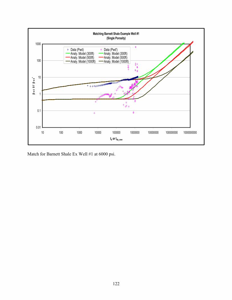
122
Matching Barnett Shale Example Well #1
(Single Porosity)
0.01
0.1
1
10
100
1000
10 100 1000 10000 100000 1000000 10000000 100000000 1000000000
td or tda_new
pwd or p
wd'
Data (Pwd) Data (Pwd')Analy. Model (300ft) Analy. Model (300ft)Analy. Model (500ft) Analy. Model (500ft)Analy. Model (1000ft) Analy. Model (1000ft)
Match for Barnett Shale Ex Well #1 at 6000 psi.
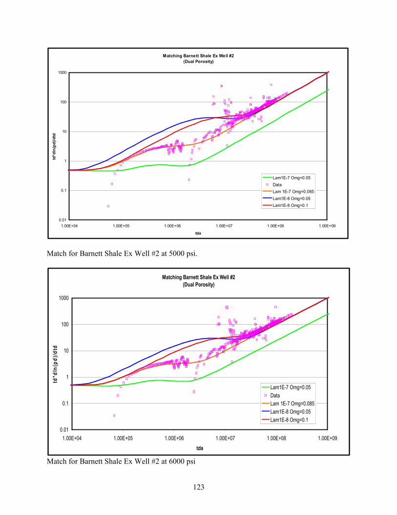
123
Matching Barnett Shale Ex Well #2
(Dual Porosity)
0.01
0.1
1
10
100
1000
1.00E+04 1.00E+05 1.00E+06 1.00E+07 1.00E+08 1.00E+09
tda
td*dln(pd)/dtd
Lam1E-7 Omg=0.05
Data
Lam 1E-7 Omg=0.085
Lam1E-8 Omg=0.05
Lam1E-8 Omg=0.1
Match for Barnett Shale Ex Well #2 at 5000 psi.
Matching Barnett Shale Ex Well #2
(Dual Porosity)
0.01
0.1
1
10
100
1000
1.00E+04 1.00E+05 1.00E+06 1.00E+07 1.00E+08 1.00E+09
tda
td*dln(pd)/dtd
Lam1E-7 Omg=0.05
Data
Lam 1E-7 Omg=0.085
Lam1E-8 Omg=0.05
Lam1E-8 Omg=0.1
Match for Barnett Shale Ex Well #2 at 6000 psi

124
APPENDIX B
The dual porosity analytic models used in this work contained a pseudosteady state interporosity
flow relationship. This is a concern for the analysis of field cases. It is necessary to use a
transient interporosity flow relationship when the matrix block size becomes relatively large
compared to the drainage radius.
Assuming a cube fracture geometry, the matrix block size for the Barnett Shale Ex Well #2 was
found to be larger than the drainage radius. Therefore, a dual porosity analytic model with
transient interporosity flow was used in addition to the pseudosteady state interporosity flow for
the Barnett Shale Ex Well #2. The match for Barnett Shale Ex Well #2 can be seen below.
Matching Barnett Shale Ex Well #2
(Dual Porosity, Transient Interporosity)
0.01
0.1
1
10
100
1000
10000
1.00E+03 1.00E+04 1.00E+05 1.00E+06 1.00E+07 1.00E+08 1.00E+09
Data
Analytic Model
This is not as good a visual match at early time as the pseudosteady state interporosity flow
model is. However, this match was achieved using 4000 psi and similar values of λ and ω that
were obtained using pseudosteady state interporosity flow.
Model
Type
Drainage
radius, re
(ft)
ω λ G/A*
Match
Term
( AkG φ ) *
Dual Porosity 500 0.05 1E-7 5.37 6.77

125
Matching Barnett Shale Ex Well #2 (Stimulation)
(Dual Porosity, Transient Interporosity)
0.1
1
10
100
1000
1.00E+03 1.00E+04 1.00E+05 1.00E+06 1.00E+07 1.00E+08
tda or tda_new
tda*dln(pd)/dtda
Analytic Model
Data
Here is the match for the stimulation performed on Barnett Shale Ex Well #2. The analytic
model used in this match has transient interporosity flow. This match was achieved with an
initial pressure of 4000 psi and similar values of λ and ω that were obtained from using
pseudosteady state interporosity flow.
Model
Type
Drainage
radius, re
(ft)
ω λ G/A*
Match
Term
( AkG φ ) *
Dual Porosity 225 0.05 7.5E-8 3.39 2.34

126
VITA
Adam M. Lewis is a native of Baton Rouge, Louisiana. He began his collegiate education at
Louisiana State University in 2001 and received his Bachelor of Science in Petroleum
Engineering in 2005. He has worked in various industry positions and geographic locals as an
intern. His technical interests include reservoir engineering, production engineering, and
petroleum geology.