Production Campaign Planning UnderLearning and Decay

Abstract

Problem definition. We analyze a catalyst-activated batch-production process with uncertainty in pro-

duction times, learning about catalyst-productivity characteristics, and decay of catalyst performance across

batches. The challenge is to determine the quality level of batches and to decide when to replenish a catalyst

so as to minimize average costs, consisting of inventory holding, backlogging, and catalyst switching costs.

Academic / Practical Relevance. This is an important problem in a variety of process industry sectors

such as food processing, pharmaceuticals, and specialty chemicals but has not been adequately studied in

the academic literature. Our paper also contributes to the stochastic economic lot-sizing literature.

Methodology. We formulate this problem as a Semi-Markov Decision Process (SMDP), and develop a

two-level heuristic for it. This heuristic consists of a lower-level problem which determines the quality of

batches to meet an average target quality, and a higher-level problem which determines when to replace

the costly catalyst as its productivity decays. To evaluate our heuristic, we present a lower bound on the

optimal value of the SMDP. This bound accounts for all costs, as well as the randomness and discreteness

in the process. We then extend our methods to multiple-product settings: an advanced stochastic economic

lot-sizing problem.

Results. We test our proposed solution methodology with data from a leading food processing company

and show our methods outperform current practice with average improvements of around 22% in costs. In

addition, compared to the stochastic lower bounds, our results show the simple two-level heuristic attains

near-optimal performance for the intractable multi-dimensional SMDP.

Managerial Implications. Our results imply three important managerial insights: first, our simulation-

based lower bound provides a close approximation to the optimal cost of the SMDP and it is nearly attainable

using a relatively simple two-level heuristic. Second, the re-optimization policy used in the lower-level

problem adequately captures the value of information and Bayesian learning. Third, in the higher level

problem of choosing when to replace a catalyst, the intractable multidimensional state of the system is

efficiently summarized by a single statistic: the probability of inventory falling below a specific threshold.

Key Words and Phrases : Campaign planning, Batch production, Stochastic economic lot siz-

ing problem, Bayesian updating, Production learning, Semi-Markov processes, Stochastic dynamic

programming

1 Introduction

Several batch production processes in the manufacturing of specialty chemical, food processing and

pharmaceutical industries use catalysts to control the characteristics of production. The product

is processed in batches of fixed volume in a reactor (or machine), which refines the product using a

catalyst and achieves a target attribute level. The effectiveness of the catalyst decays with usage.

Every catalyst has an optimal life span; it may be pushed too far or prematurely replaced if a proper

strategy is not employed. The producer must choose efficient policies to minimize the expected

costs, including inventory-related costs and the price of the catalysts. This is an important problem

found in several settings in the process industry sector (Casas-Liza et al. 2005, Liu et al. 2014),

but has been modeled as a single-stage deterministic problem, while the problem is dynamic in

nature. By considering the dynamic problem, this paper addresses the limitations in the literature

and more accurately represents the actual decision process.

The sequence of batches that are exposed to the same catalyst at different stages of decay are

referred to as a “campaign” of batches. Batches within a campaign can be mixed to meet the

average attribute level target. Mixing batches allows for the optimal exploitation of the potential

of a catalyst as it offers more flexibility in determining the duration of batches. The productivity

of the catalyst decays as it is used across more batches, until at some point the producer has to

switch to a new catalyst and incur the associated switch-over costs. The initial productivity of a

new catalyst is a random value drawn from a known distribution, estimated from historical data.

We cannot observe the exact productivity of the current catalyst due to random shocks experienced

by each batch. The noisy observations on each batch allow us to update our information about

the productivity of the catalyst through Bayesian updating. Our goal is to plan the duration of

the batches and decide when to replenish a catalyst so as to minimize the expected average cost

which includes inventory holding, backlogging, and catalyst-switching costs. We first explore the

single product case and then extend the results to multiple products. With multiple products, in

addition to batch planning and catalyst replenishment decisions, we must also decide which product

to produce next.

We formulate the single-product batch-production planning problem with learning and decay

as a semi-Markov, average-cost model. We decompose it into two levels to make it tractable.

1

The lower-level problem plans the duration of batches within the current campaign to maximize

the efficiency of the catalyst, while satisfying the target average attribute level. The higher-level

problem is a binary decision after each batch: whether or not to end this campaign and switch to a

new catalyst. The lower level is formulated as a stochastic dynamic programming problem, similar

to the Bayesian decision model by Mazzola and McCardle (1996), which had a production learning

curve (as opposed to our decay curve). Despite the similarities of the models, our problem has an

additional constraint (the average attribute level constraint), which adds one more dimension to the

state space. Therefore we adopt a re-optimization policy that relies on learning to take care of itself

and show that it has near-optimal performance. The higher-level problem is to design a control

policy mapping the state space to a binary control variable- changing the catalyst or continuing.

The objective is to minimize the average costs (switchover, backlogging and inventory). The state

space consists of the current inventory level, current consumption of the catalyst (measured by the

total time the current catalyst has actively been used to produce batches), and the current belief

regarding the catalyst productivity parameter. Solving for an optimal mapping from the state

space to the decision variable is intractable. We propose a heuristic policy to approximately solve

this problem.

To evaluate the performance of this two-level heuristic, we obtain a lower bound on the optimal

performance of the original integrated decision process. This bound simultaneously accounts for

costs, randomness, and the discrete nature of the process. We also compare the performance of

our heuristic with the fixed cycle policy that is currently practiced by the leading food-processing

company that provided the motivation of this work.

We then extend our model to consider the multi-product case with uncertainty in production

times. This can be regarded as a Stochastic Economic Lot Scheduling Problem (SELSP) with

fixed batch sizes, learning and decay. Due to the complexity of this problem, we solve this using a

dynamic model-based heuristic. Vaughan (2007) compares dynamic vs. cyclical policies for SELSP

problems and shows that in many cases cyclical policies perform better than dynamic policies.

However, in our context cyclical policies suffer from delayed reaction towards backlogged demand;

a dynamic policy is needed to recognize and attend to the critical product that would otherwise

cause large backlogging costs. The model-based heuristic is benchmarked with a practitioners

heuristic used by a large food processing company. We also develop a lower bound on this problem

2

to evaluate the performance of these heuristics.

The literature related to our work can be classified by problem type: single product and multi-

product. The single product problem is related to the single item stochastic economic lot sizing

problem. Levi and Shi (2013) review a wide selection of the single-item SELSP literature, many of

which show that (s, S) policies are optimal under specific problem configurations. However, in our

problem (s, S) policies are not feasible because depending upon the current catalyst productivity

and the decaying nature of the catalyst, it may not be possible to produce up to S. Another

important feature of our problem is that we learn about the current productivity of the catalyst by

observing the performance in previous batches. This learning is used to predict catalyst performance

and production times of future batches. Levi and Shi (2013) consider a related stochastic lot sizing

problem and include the prediction of future demand (got from observations in previous periods) in

the current decision process. They propose a randomized cost-balancing policy to decide when and

how much to order. However, their problem considers uncapacitated orders and discrete periods,

while we consider production that is constrained by the limited productivity of a catalyst, and

our decision epochs are randomly determined by batch completion times. The relevant literature

for multi-product models include work on the SELSP (Winands et al. 2011) and economic lot

sizing models under production decay (Casas-Liza et al. 2005, Liu et al. 2014). To the best of

our knowledge, ours is the first paper to consider all these settings together. In terms of solution

methods for the SELSP, work that uses dynamic approaches to solve the SELSP includes Rajaram

and Karmarkar (2002), Dusonchet and Hongler (2003), and Wang et al. (2012). In terms of

application, Rajararam and Karmarkar (2004) also consider a campaign planning problem applied

to the food-processing industry. However, none of the methods used in these papers can be used

to solve the problem considered in this paper due to batching, learning across batches and decay

in performance of the catalyst.

In this context, our paper makes the following contributions. First, to the best of our knowledge,

this is the first paper to consider the campaign planning problem under production time uncertainty,

learning and decay. As previously discussed, this is an important problem that has not been

adequately studied in the academic literature. Second, we formulate this problem as a semi-Markov

decision process, incorporating key aspects of this problem which include uncertainty in production

time, learning about productivity characteristics and decay in catalyst performance. Third, we

3

develop efficient, near optimal solution methods to solve this problem. In addition, our approach

to find lower bounds by associating a continuous state space dynamic programming problem with a

similar but regenerative process can be applied to other stochastic dynamic programming problems.

Fourth, we validate our model and solution methods with real data from the process industry. Fifth,

we provide several insights which could be useful for practitioners in other industries which have a

similar production setting.

The remainder of this paper is organized as follows. We begin by formulating the single product

problem as a Semi-Markov Decision Process (SMDP) in §2, followed by lower bounds on the optimal

cost of the SMDP in §3. In §4 we present the solution methodology based on a two-level heuristic

which involves decomposing the problem into two level of decision making. To benchmark the

two-level heuristic, we also provide a practitioner’s heuristic that is currently employed at a large

food processing company. We extend our methodology to the multiple product case in §5. In §6

we compare the performance of the heuristics and lower bound on real factory data and present

managerial insights. Conclusions and future research directions are provided in §7.

2 Model Formulation

Consider a batch production process in which the present state of the production system is defined

by the current inventory level and the state of the catalyst currently in use (to be explained in

further detail). Based on this information, the firm must decide whether to replace the current

catalyst and start a new campaign, or to produce another batch with the current catalyst and

determine the attribute level of the next batch. We denote the current inventory level as I and

treat it as a continuous variable. Further, for ease of exposition and without loss of generality

we measure inventory as batches and assume that the batch size is equal to 1. That is, inventory

replenishes by discrete counts but depletes continuously with a constant per-unit-time demand.

Next, we define the following parameters and variables:

Parameters:

d : constant demand rate (batches/unit-time).

CB: backlogging cost ($/batch/unit-time).

CI : inventory holding cost ($/batch/unit-time).

4

CS : cost of changing a catalyst ($).

ts : switch-over time required to change a catalyst (unit-time).

Stochastic variables:

b : inverse productivity parameter of a catalyst

zi: random shock observed by the catalyst while producing batch i.

z = [z1, z2, ..., zN ]: combining the zi’s of a campaign into one vector.

Decision variables:

N : number of batches produced by a catalyst, i.e. the length of a campaign.

qi : The attribute level of the i’th batch in a campaign (normalized, dimensionless).

The decision variables imply the following intermediary variables:

q=[q1, q2, ..., qN ] : vector of attribute levels of all batches produced by a catalyst.

Qi =∑i−1

j=1 qj : sum of all attribute levels up to the beginning of batch i.

ti : time spent by batch i in the reactor (unit-time/batch).

Ti =∑i−1

j=1 tj : total consumption of the catalyst up to batch i (unit-time).

We define the following functions:

γ(b): a density function representing the current belief distribution over possible values of the

parameter b. The prior belief is γ0(b).

τ(q, b, z) : time spent on a catalyst with production schedule q and inverse productivity b. Takes

random values based on the realizations of the random shocks zi. (unit-time)

τ∗(N): expected optimal time it would take to produce N batches in a campaign, given full

information of b and z. (unit-time)

g(I, τ): total inventory holding and backlogging cost during time length τ , where the inventory

level starts at I and ends at I − τd. (unit-cost).

A batch that enters the reactor begins at an initial attribute level. This attribute level declines

as the batch is refined. The time it takes to process batch i is denoted by ti and is determined

by the consumption of the catalyst Ti, inverse productivity of the catalyst and the random shock

observed (b+ zi), and the target attribute level qi. The three elements have separable effect on the

5

duration of the batch, thus ti is related to these elements via:

ti = k(Ti)(b+ zi)f(qi), (1)

where k is a monotone increasing function that defines the dependancy of the processing time of

the ith batch on the total consumption of the catalyst up to the starting time of this batch. The

inverse productivity parameter b comes from a known distribution with mean µb and variance σ2b ,

and it only takes positive values. It varies by catalyst but is fixed across batches produced by

a partcular catalyst. The shocks zi are iid variables with mean zero and a known distribution.

We assume b + zi is always positive. Finally, f(qi) is a convex decreasing function to capture the

increases in time it takes to purify batch i and reduce attribute qi ≥ 0 from its initial starting level.

This function is convex because of the process characteristic: the lower the attribute level qi, the

longer it takes for further reductions from this level.

Equivalently, to show the attribute level of a batch as a function of the time it spends in the

machine, we have:

qi = f−1( tik(Ti)(b+ zi)

). (2)

For example, if k(T ) = T + 1 and f(q) = −ln(q), the relation between q and t would take the form:

qi = exp(− ti

(Ti + 1)(b+ zi)

). (3)

The decision to be made prior to placing the next batch inside the reactor is to either choose

a target attribute level qn+1 for the next batch, or to end the current campaign and replace the

catalyst. We do not allow the option of removing a batch before meeting the target attribute level.

The belief distribution γ(b) is updated by observing the pair (ti, qi)|Ti after each batch. At the

end of the campaign and after replacing the catalyst, the new inventory level will be:

I ′ = I − (τ(q, b, z) + ts)d+N. (4)

Due to the randomness of b and zi, the new state (I ′) will be a random function of the old

state (I) and the vector of actions qi summarized in q. The campaign time (τ(q, b, z) ) is also a

random function of q. The cost of this transition is the inventory and backlogging cost during the

6

time τ(q, b, z) + ts plus the cost of changing the catalyst. Due to the pooling strategy, in which

the batches in a campaign are mixed by the producer, the batches produced by a catalyst are not

available in the sales inventory until the catalyst is changed. We make two assumptions regarding

the inventory and backlogging costs:

(i) Backlogging costs occur if the total demand during the catalyst lifespan (i.e. (τ(q, b, z) + ts)d)

exceeds the initial inventory level I.

(ii) The batches that have not been pooled and prepared for sale do not induce inventory costs.

Let the function g(I, τ) represent the total inventory and backlogging costs during a time span

of τ when the starting inventory is I and no batches are added to the inventory during τ . To derive

g(I, τ), we need to consider three cases. First, if we do not run out of inventory during time τ ,

we incur only inventory holding costs which are proportional to the average inventory (I − τd/2)

multiplied by the duration of the time horizon (τ). Second, if we start from a positive inventory

level but run out during time τ , we incur both inventory and backlogging costs. The length of time

with positive inventory is I/d and the average inventory level during this time is I/2. The final

inventory is I−τd, hence the length of time with backlogging is (I−τd)/d and average backlogging

during this time is (I − τd)/2. Finally, if we start from a negative inventory, the only cost during

τ will come from backlogging and is computed similarly to the case where we only incur inventory

holding cost. Thus g(I, τ) is computed as:

g(I, τ) ,

τ(I − τd/2)CI if I − τd ≥ 0

I2/2d× CI − CB(I − τd)2/2d if I ≥ 0 & I − τd < 0

−τ(I − τd/2)CB if I < 0.

(5)

In order to define the objective function, we first define the term “cycle”. A cycle refers to the

length of time between the ending of two subsequent campaigns. A cycle of duration τj consists of

a campaign with length τ cj = τ(qj , bj , zj) + ts and an idle time τ0j before setting up the campaign.

During a cycle no batches are added to the inventory, hence the realized cost during cycle j is

g(Ij , τj), where the cycle starts at inventory Ij . This problem can be formulated as a semi-Markov

average-cost problem with transition cost g(Ij , τj). The cost function for the average-cost problem

7

is:

limR→∞

1∑Rj=1 τj

E{ R∑j=1

[CS + g(Ij , τj)]}. (6)

We formulate the problem of minimizing (6) as a Bayesian stochastic dynamic program. A

control policy maps the state space to a decision of either choosing a target attribute level qn+1 for

the next batch, or ending the current campaign. The state space consists of the current inventory

level (I), number of batches produced so far in the current campaign (n), current belief distribution

γ(b), the total consumption of the current catalyst (T ), and the cumulative attribute level of the

n batches produced in the current campaign (Q). For simplicity and conformance to practice, we

allow idle time periods only immediately prior to setting up campaigns. We consider two types of

states; the first is when a campaign is in process while the second is when a campaign has finished

and the next campaign has not yet been set up. Denote the differential costs of the first state by

h(I, n,Q, T, γ(b)) and the differential costs of the second states by w(I). The optimal average cost

of the problem is denoted by λ∗, which is treated as a variable in the Bellman equation. The SMDP

is formalized as follows.

(SMDP ) h(I, n,Q, T, γ(b)) = min{Cs + w(I + n),

minqn+1

Etn+1|qn+1[h(I − tn+1d, n+ 1, Q+ qn+1, T + tn+1, γ

′(b)) + g(I, tn+1)− λ∗tn+1]}

w(I) = mint≥ts{h(I − td, 0, 0, 0, γ0(b))− λ∗t}.

(7)

Here γ0(b) is the prior belief distribution on b (the distribution from which b is drawn), γ′(b) is

the belief distribution over b after observing the next batch. The time for the next batch, denoted

by tn+1, is random and depends on qn+1. The first term in the minimization represents the decision

to switch to a new catalyst, and the second term represents the decision to produce another batch

with the current catalyst, in which case the next target attribute level qn+1 must also be chosen.

As a consequence of the curse of dimensionality, this problem is too complex to be approached

directly. Therefore we construct a two-level heuristic described in §4 to solve this problem. To

evaluate the performance of this heuristic, we next present a procedure to compute lower bounds

on the optimal average cost λ∗ of the SMDP. Some results from the lower bounds will be used to

develop the two-level heuristic.

8

3 Lower Bounds

To compute a lower bound on the optimal average cost of the SMDP, we first consider a deterministic

version of the problem and compute an associated lower bound. This lower bound does not consider

the cost of randomness and discrete production and is usually a loose bound. However, we consider

this bound for two reasons: (i) the resulting (loose) lower bound is used to construct a tighter

stochastic lower bound, and (ii) this tractable model structure and the respective insights are used

to construct our heuristic solution in §4. We then present a stochastic lower bound which accounts

for discrete production and randomness of the process. This bound resolves the inadequacies of the

deterministic bound which result from ignoring discreteness and randomness, but still ignores the

uncertainty on production parameters and assumes perfect knowledge of the (randomly) realized

catalyst productivity of each batch; in other words it assumes that we can optimally exploit the

productivity of a catalyst as if we had full information. Such clairvoyant bounds have been used in

the stochastic programming literature (Ciocan and Farias 2012). Clairvoyant bounds underestimate

optimal costs because they assume more accurate learning than is actually possible (Brown and

Smith 2013). However, we found in our computational analysis that this bound performed quite

well in our problem context, as we have considered randomness and discrete production of the

process in computing this bound.

3.1 Deterministic Lower Bound

The deterministic version of the problem is formed by assuming that a campaign with N batches

always takes a deterministic amount of time equal to τ∗(N), where τ∗(N) is the expected optimal

time it would take to produce N batches in a campaign, given full information of b and z, or

formally:

τ∗(N) = Eb,z minq

[τ(q, b, z)]. (8)

To relax the integer constraint on N and allow continuous production, we define τ∗(N) for

non-integer values of N by a weighted average of the production time of dNe and bNc, the two

closest integers to N .

τ∗(N) , (dNe −N)τ∗(bNc) + (N − bNc)τ∗(dNe) N non-integer. (9)

9

To see the reasoning behind equation (9), note that one way to produce N batches per campaign

on average is to produce bNc batches in (dNe − N) fraction of the campaigns and dNe batches

in (N − bNc) fraction of the campaigns, leading to an average time of (dNe −N)τ∗(bNc) + (N −

bNc)τ∗(dNe) per campaign. The function τ∗(N) is piecewise linear and convex. It is convex

because for an integer N , the following inequality holds as a result of decaying productivity:

τ∗(N + 1)− τ∗(N) ≥ τ∗(N)− τ∗(N − 1). (10)

Let Tcyc be the total length of a cycle, including the idle time and the campaign time.

Proposition 1 The following Economic Production Quantity (EPQ) problem provides a lower

bound on λ∗, the optimal average cost of the SMDP.

[EPQ] λEPQ = minTcyc,I

Cs + g(I, Tcyc)

Tcyc

s.t. τ∗(Tcycd) + ts ≤ Tcyc.(11)

All proofs are provided in the online supplement §A. Here, the objective of the EPQ is to

minimize the average cost during a fixed cycle. The decision variables Tcyc and I denote the length

and the starting inventory of the cycle, respectively. The total cost during a cycle is equal to a

one-time switching cost, plus inventory holding and backlogging costs during the cycle (g(I, Tcyc)).

A total of Tcycd batches are produced in a campaign to match the total demand during the length

of the cycle. The constraint ensures that the total time required to produce Tcycd batches (i.e.

τ∗(Tcycd)) plus the setup time is less than or equal to the length of the cycle. We define the

following parameters based on the solution to (11):

T ∗cyc: optimal cycle length in (11).

TM : largest cycle length satisfying the production constraint in (11).

Tm: smallest cycle length satisfying the production constraint in (11).

N∗ , T ∗cycd: total demand during T ∗cyc. It is similar to the optimal order quantity Q∗ in an

unconstrained EOQ model.

10

I: optimal inventory at the beginning of each cycle (i.e. after adding to inventory the batches

produced in the previous campaign).

I , I −N∗: lowest inventory reached at the end of a cycle, just before the newly produced

batches are added.

CIB , CICBCI+CB

: “balanced” inventory holding and backlogging cost per unit time in an EPQ

with backlogging (will be discussed shortly).

C0s : the supremum value of all Cs such that the constraint in (11) is not binding at the

optimal solution (will be discussed shortly).

Given a cycle length Tcyc, inventory will be positive for a fraction of the cycle, and for the

remaining time inventory will be negative. We show that the optimal fraction of time where

inventory is positive and where it is negative are proportional to CB and CI respectively.

Proposition 2 The optimal I can be derived as a function of Tcyc and replaced in the objective

function. The resulting objective function is convex in Tcyc.

Corollary 2.1 Problem EPQ becomes a convex optimization problem in the single variable Tcyc.

In the proof of Proposition 2 (in the online supplement) we see that the objective over Tcyc

becomes CsTcyc

+(CICBCI+CB

)Tcycd

2 , which is similar to an EPQ without backlogging in which CIB ,

CICBCI+CB

has replaced the inventory holding cost. The parameter CIB is interpreted as the balanced

inventory cost (holding and backlogging) per unit time when the cycle length is optimally allocated

between positive and negative inventory. The optimal production quantity in the unconstrained

EPQ problem is

Nu =

√2CSd

CIB. (12)

If T ucyc = Nu/d satisfies the production constraint, then the constraint is not binding and T ucyc

is optimal for problem (11). In this case the following relations would hold:

N∗ = Nu =

√2CSd

CIB,

I =CI

CI + CBN∗,

λEPQ =√

2CIBCSd = ICB = N∗CIB.

(13)

11

In order for T ucyc to be feasible (hence optimal) we must have Tm ≤ T ucyc ≤ TM . If T ucyc does not

satisfy the constraint, then the constraint is binding at the optimal T ∗cyc because by Proposition 2

the objective function is convex in Tcyc. If T ucyc < Tm, then T ∗cyc = Tm, and if T ucyc > TM , then

T ∗cyc = TM .

3.2 Stochastic Lower Bound

The solution to EPQ gives a lower bound for the original problem, but it does not account for

the cost of randomness and discrete production. To obtain a tighter bound, we use the EPQ and

define a stochastic process that is similar to the actual production process, but is regenerative and

hence more tractable. The optimal cost of this regenerative process is a tighter lower bound than

the EPQ bound for the original problem.

Proposition 3 The differential cost function w(I) defined in (7) has a global minimizer I∗.

According to Proposition 3, the level I∗

is the ideal inventory to have at the beginning of a

cycle. However, it is not necessarily optimal to immediately start the next campaign at I∗

and we

might allow some idle time. This is shown in Proposition 4.

Proposition 4 There exists an inventory level I∗0 ≤ I∗, such that if the inventory level at the

beginning of a cycle is I∗, it is optimal to delay the campaign setup till inventory falls to I∗0 .

We now define a regenerative process by modifying the original process as follows:

I) Production always starts at I∗0 .

II) If the inventory level I at the end of a campaign is less than I∗0 , the inventory level is instantly

raised to I∗0 at a cost of λEPQtI0I − g(I∗0 , tI0I), where λEPQ is the optimal cost of problem

(11) and tI0I = (I∗0 − I)/d.

III) If the inventory level I at the end of a campaign is greater than I∗0 , the inventory level is

instantly dropped to a level I ′ of choice (I ≥ I ′ ≥ I∗0 ) and then production is idled until

inventory reaches I∗0 .

12

Proposition 5 There exists a regenerative process satisfying I-III that has a lower average cost

than the optimal cost of the original process. As a result, the optimal average cost of the regenerative

process is less than the optimal average cost of the original process.

In the regenerative process, all campaigns start at I∗0 , hence it is more tractable than the

original process. However, computing the optimal cost of the regenerative process is still not

straightforward. In the Appendix we present an algorithm to compute a lower bound on the

optimal performance of the regenerative process given I∗0 . A lower bound on the optimal cost of

the original process can then be obtained by a line search over values of I∗0 .

4 Heuristics and Upper Bounds

In this section, we present a two-level heuristic to solve the SMDP. This provides an upper bound

on the value of the SMDP. To benchmark the performance of this heuristic, we also describe a

practitioners heuristic currently employed at a large food processing company.

4.1 Two-level Heuristic

In the two-level heuristic, we decompose the campaign planning problem with learning and decay

represented by the SMDP into two levels: a lower level problem at the batch level, determining the

duration of batches in a campaign, and a higher level problem at the campaign level, determining

when to end a campaign. These levels are defined as:

• Level 1: Batch planning- Choose the attribute level qn+1 of the next batch.

• Level 2: Catalyst switching- While batch n is inside the reactor, use a control policy to decide

whether to change the catalyst after this batch, or to move on to batch n+ 1.

We next describe the solution method for each level.

Level-1: Batch Planning

In batch planning, we focus on minimizing the campaign duration for a given number of batches N .

We minimize the campaign duration because it offers more buffer time and hence more flexibility.

The objective is to minimize TN + tN such that the average attribute level constraint is satisfied.

13

The number of batches N is tentatively chosen as the expected number of batches in the campaign

which depends on the higher-level policy discussed in the next subsection. For ease of exposition

and without loss of generality, the attribute level is normalized such that the required average

attribute level is less than or equal to 1. Hence the average attribute level constraint becomes:

N∑i=1

qi ≤ N. (14)

With this constraint, the state space should include the cumulative attribute level. After com-

pletion of batch i−1, a decision qi is made for the ith batch, given the current state of the campaign

[Qi, Ti, γ(b)]. The resulting stochastic DP is represented by the following Bellman equation:

vi(Qi, Ti, γ(b)) = minqi

[Ezi,b{(b+ zi)k(Ti)f(qi) + vi+1(Qi + qi, Ti + (b+ zi)k(Ti)f(qi), γ′(b))}], (15)

where γ(b) is the current belief distribution on the parameter b and γ′(b) is the updated belief after

observing the random outcome of b + zi. We use a standard Bayesian updating procedure to get

γ′(b): each period based on our observation of the pair (qi, ti), we observe the implied productivity

bi , b+ zi through

ti = bik(Ti)f(qi)⇒ bi = ti/k(Ti)f(qi).

We use this observation along with the known density of zi (i.e. κ(zi)) to update γ(b) according to

γ′(b) ∝ γ(b)κ(bi − b). Here the current belief γ(b) acts as the prior belief, and the new probability

density for b, according to Bayes’ rule, is proportional to the previous density multiplied by the

likelihood of observing bi conditional on b (i.e. κ(bi − b)).

An analytical closed form solution to this problem is not available in general, and the contin-

uous multidimensional state space of this stochastic Bayesian DP problem makes it intractable to

numerically find an optimal policy (Mazzola and McCardle 1996). Hence we approach this problem

with the following re-optimization heuristic: first we find the vector q that minimizes the expected

campaign length Eb,z{τ(q, b, z)}, ignoring the fact that q can be adjusted in the future. After

the first batch q1 is completed, we incorporate learning by updating γ(b) and re-optimizing the

remaining batches 2 through N of q. We then implement the revised second batch, and repeat.

The re-optimization policy does not directly anticipate the value of information in its decision

14

process. In the online supplement §B we set up a tractable 3-batch example and compare the

re-optimization policy with the optimal policy. We make three important observations:

i) In all problem settings considered, the choice of q1 under the re-optimization policy is very

close to the optimal choice of q1 .

ii) The resulting average campaign time is almost identical under the two policies (they are within

1% of each-other in all considered problem settings).

iii) Both policies attain near-optimal exploitation of the catalyst, as if full information on b were

available apriori (in every problem setting, the expected campaign duration under the two

policies is within 2% of the minimum campaign duration).

In addition, our computational results in §6 show that our two-level heuristic achieves near-

optimal costs, implying that the re-optimization policy adequately captures the dynamic value of

information in this problem.

With the re-optimization policy in place, we are interested in understanding how the chosen

q will differ from the myopic policy of having every batch meet the target attribute level (i.e.

q = [1, 1, ..., 1]). Note that a smaller qi implies that batch i has a bigger contribution to satisfying

the average attribute level constraint (14). Therefore, we interpret assigning a smaller qi to batch

i as placing a higher “load” on batch i. We are interested in whether it is better to place higher

load (i.e. smaller qi) on the production of the first batches (while the productivity of the catalyst

is still high) and leave a lower load on the concluding batches, or conversely place a lighter load on

the initial batches to avoid an overly decayed catalyst when it reaches the final batches. As shown

in Proposition 6, this depends on the form of k(Ti), the function which defines the dependency

of the productivity decay rate (equivalently, the rate of increase in processing time) on the total

consumption. Denote q∗ = [q∗1, ..., q∗N ] as the solution to arg minqEb,z{τ(q, b, z)}.

Proposition 6 (i) If k(T ) is convex in T , then there exists at least one optimal solution where

q∗i ≥ q∗i+1. Further, if k(T ) is strictly convex, there are no optimal solutions where q∗i ≤ q∗i+1.

(ii) If k(T ) is concave in T , then there exists at least one optimal solution where q∗i ≤ q∗i+1. Further,

if k(T ) is strictly concave, there are no optimal solutions where q∗i ≥ q∗i+1.

15

(iii) If k(T ) is an affine function, then q∗i = q∗i+1 for all i.

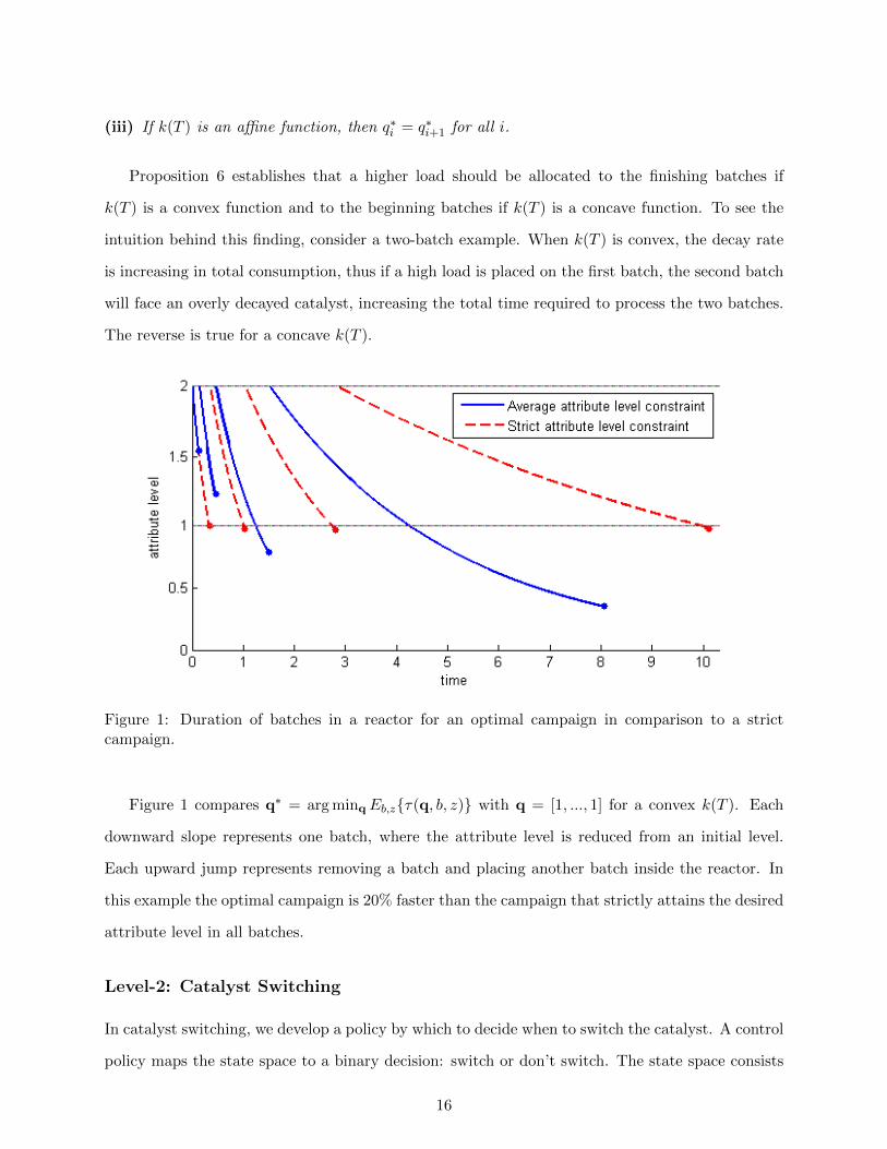
Proposition 6 establishes that a higher load should be allocated to the finishing batches if

k(T ) is a convex function and to the beginning batches if k(T ) is a concave function. To see the

intuition behind this finding, consider a two-batch example. When k(T ) is convex, the decay rate

is increasing in total consumption, thus if a high load is placed on the first batch, the second batch

will face an overly decayed catalyst, increasing the total time required to process the two batches.

The reverse is true for a concave k(T ).

Figure 1: Duration of batches in a reactor for an optimal campaign in comparison to a strictcampaign.

Figure 1 compares q∗ = arg minqEb,z{τ(q, b, z)} with q = [1, ..., 1] for a convex k(T ). Each

downward slope represents one batch, where the attribute level is reduced from an initial level.

Each upward jump represents removing a batch and placing another batch inside the reactor. In

this example the optimal campaign is 20% faster than the campaign that strictly attains the desired

attribute level in all batches.

Level-2: Catalyst Switching

In catalyst switching, we develop a policy by which to decide when to switch the catalyst. A control

policy maps the state space to a binary decision: switch or don’t switch. The state space consists

16

of the current inventory level (I), number of batches produced so far in the current campaign (n),

current belief distribution of b (γ(b)), and the total consumption of the current catalyst (T ). The

Bellman equation for this average-cost problem is an approximation to the SMDP, where the Q

dimension is removed from the state space and the decision variable is binary (instead of being a

continuous choice of qn, which is now handled by the lower-level problem).

h(I, n, T, γ(b)) = min{Cs + w(I + n),

Etn+1 [h(I − tn+1d, n+ 1, T + tn+1, γ′(b)) + g(I, tn+1)− λ∗tn+1]}

w(I) = mint≥ts{h(I − td, 0, 0, γ0(b))− λ∗t}.

(16)

The state space is multidimensional and has continuous elements. Even if we remove the ele-

ments of learning and decay, the state space is still too large to obtain exact solutions (Loehndorf

and Minner 2013), even numerically. Hence we propose an approximate policy to efficiently sum-

marize the large state of the system and apply it in a simple decision rule.

The intuition behind our heuristic is to follow as closely as possible the optimal policy of

the deterministic process suggested by the solution to the EPQ. Let I and T ∗cyc be the optimal

solution to (11). Define I , I − T ∗cycd and I0 , I + [τ∗(T ∗cycd) + ts]d. In the absence of randomness

and discreteness, we would like the inventory level at the beginning of a cycle to be I, idle the

process until inventory reaches I0, at which time we set up a campaign and produce batches until

inventory is at I. The batches produced return inventory to I. However, in the discrete-production

stochastic process this does not necessarily happen. At some point we expect that if we produce

another batch, the inventory level at the end of that batch will be lower than I, which would result

in excess backlogging costs. On the other hand, if we do not produce another batch and switch the

catalyst before reaching the optimal level of I, it would result in higher average switching costs,

and possibly higher inventory costs in the next cycle.

To choose between these options, we propose to switch before inventory gets to I only if the

probability of falling below inventory I after the next batch is greater than some threshold Ψ. The

probability P [In+1 < I] is calculated using the distribution of zn and the current belief over b:

17

P [In+1 < I] = P [I − tn+1d < I] = P [tn+1d > I − I]

= P [(b+ zn+1)k(Tn+1)f(qn+1)d > I − I]

= P[b+ zn+1 >

I − Ik(Tn+1)f(qn+1)d

].

(17)

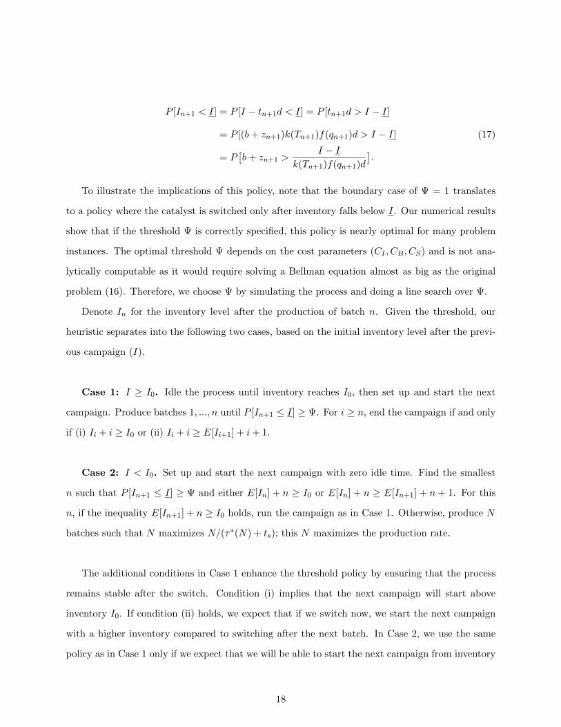
To illustrate the implications of this policy, note that the boundary case of Ψ = 1 translates

to a policy where the catalyst is switched only after inventory falls below I. Our numerical results

show that if the threshold Ψ is correctly specified, this policy is nearly optimal for many problem

instances. The optimal threshold Ψ depends on the cost parameters (CI , CB, CS) and is not ana-

lytically computable as it would require solving a Bellman equation almost as big as the original

problem (16). Therefore, we choose Ψ by simulating the process and doing a line search over Ψ.

Denote In for the inventory level after the production of batch n. Given the threshold, our

heuristic separates into the following two cases, based on the initial inventory level after the previ-

ous campaign (I).

Case 1: I ≥ I0. Idle the process until inventory reaches I0, then set up and start the next

campaign. Produce batches 1, ..., n until P [In+1 ≤ I] ≥ Ψ. For i ≥ n, end the campaign if and only

if (i) Ii + i ≥ I0 or (ii) Ii + i ≥ E[Ii+1] + i+ 1.

Case 2: I < I0. Set up and start the next campaign with zero idle time. Find the smallest

n such that P [In+1 ≤ I] ≥ Ψ and either E[In] + n ≥ I0 or E[In] + n ≥ E[In+1] + n + 1. For this

n, if the inequality E[In+1] + n ≥ I0 holds, run the campaign as in Case 1. Otherwise, produce N

batches such that N maximizes N/(τ∗(N) + ts); this N maximizes the production rate.

The additional conditions in Case 1 enhance the threshold policy by ensuring that the process

remains stable after the switch. Condition (i) implies that the next campaign will start above

inventory I0. If condition (ii) holds, we expect that if we switch now, we start the next campaign

with a higher inventory compared to switching after the next batch. In Case 2, we use the same

policy as in Case 1 only if we expect that we will be able to start the next campaign from inventory

18

above I0. Otherwise, we produce at the maximum production rate to bring the process back up to

stable conditions.

4.2 Practitioner’s Heuristic

To benchmark the two-level heuristic, we compare it with a practitioner’s heuristic that was im-

plemented as part of a broader project described in Rajaram et al. (1999). The decision variables

are t∗, how long to leave each batch in the reactor, and N , the maximum number of batches in a

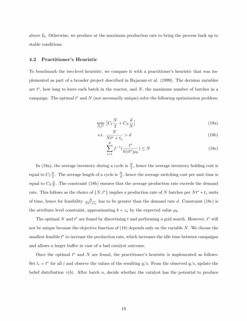
campaign. The optimal t∗ and N (not necessarily unique) solve the following optimization problem:

minN,t∗

[CIN

2+ CS

d

N

](18a)

s.t.N

Nt∗ + ts> d (18b)

N∑i=1

f−1(t∗

k(it∗)µb) ≤ N (18c)

In (18a), the average inventory during a cycle is N2 , hence the average inventory holding cost is

equal to CIN2 . The average length of a cycle is N

d , hence the average switching cost per unit time is

equal to CSdN . The constraint (18b) ensures that the average production rate exceeds the demand

rate. This follows as the choice of {N, t∗} implies a production rate of N batches per Nt∗+ ts units

of time, hence for feasibility NNt∗+ts

has to be greater than the demand rate d. Constraint (18c) is

the attribute level constraint, approximating b+ zn by the expected value µb.

The optimal N and t∗ are found by discretizing t and performing a grid search. However, t∗ will

not be unique because the objective function of (18) depends only on the variable N . We choose the

smallest feasible t∗ to increase the production rate, which increases the idle time between campaigns

and allows a larger buffer in case of a bad catalyst outcome.

Once the optimal t∗ and N are found, the practitioner’s heuristic is implemented as follows:

Set ti = t∗ for all i and observe the values of the resulting qi’s. From the observed qi’s, update the

belief distribution γ(b). After batch n, decide whether the catalyst has the potential to produce

19

another batch with tn+1 = t∗ while preserving the average attribute-level constraint:

n+1∑i=1

f−1(t∗

k(it∗)(b+ zi)) ≤ n+ 1. (19)

Given the current information, use the expected value of b+ zn (i.e. E[b|γ(b)]) to evaluate (19);

produce another batch if and only if∑n+1

i=1 f−1( t∗

k(it∗)E[b|γ(b)]) ≤ n+ 1 and n+ 1 ≤ N .

If the prediction is wrong and the next batch violates the constraint, stop the current campaign

and incur a rework cost. Once the campaign is ended, the catalyst is replaced and the new batches

are released to inventory.

Observe that this heuristic does not allow for deliberate backlogging and is designed for the

settings where CB � CI ; it does not provide a fair benchmark when CB and CI are comparable.

To enhance this heuristic and provide a fair benchmark in all settings, we replace the cost term

CI in (18) by CIB = CICB/(CI + CB) which represents the optimal balance between inventory

holding and backlogging costs (see §3.1). To optimally balance these costs, instead of starting

and ending the cycles at I = N and I = 0, we start and end the cycles at I = N CBCI+CB

and

I = −N CICI+CB

respectively. Finally, since t∗ is chosen as the smallest feasible value for the chosen

N , the production rate will be higher than the demand rate. Therefore, idle times are chosen such

that the cycles start and finish at these inventory levels.

5 Multiple Products

We now consider a setting where multiple products are produced on a single reactor. Each product

has its own fixed demand rate, backlogging costs, and inventory holding costs. This problem is

now a stochastic economic lot sizing problem with switching costs, batch production, learning and

decay.

During the production of a given campaign, after each batch is produced, a decision must be

made: continue this campaign and produce another batch of the current product, or finish this

campaign, add the produced batches to inventory, and start a new campaign. Note that only one

type of product can be produced in a campaign. After a campaign is finished and the produced

batches are added to inventory, the next decision is which product to produce next and how much

idle time, if any, to allow. These decisions are based not only on the number of batches produced

20

n, the total consumption of the catalyst T , and the current belief distribution γ(b) over the inverse

productivity parameter b for the current product, but also on the inventory level I of all the

products. We extend the ideas discussed in the single product setting to obtain a lower bound and

a heuristic for the multiple product setting.

5.1 Lower Bound

Let R be the total number of products. We modify the previously introduced parameters and

variables by adding indices r (or superscripts, for inventory variables) to denote the product type.

A deterministic lower bound on the optimal performance of the stochastic system is to assume

that each product undergoes an EPQ process independent of the others, except that the sum of

fractions of time that the machine is busy cannot be greater than 1.

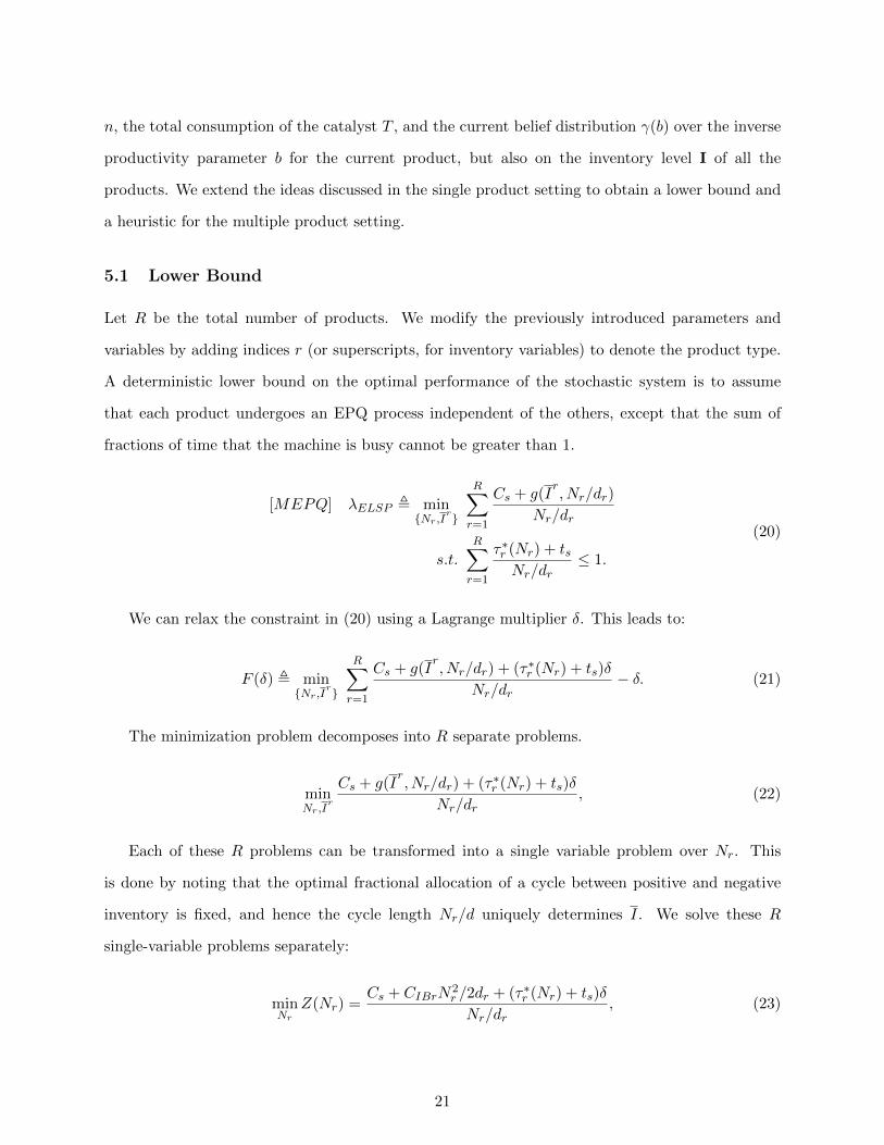
[MEPQ] λELSP , min{Nr,I

r}

R∑r=1

Cs + g(Ir, Nr/dr)

Nr/dr

s.t.

R∑r=1

τ∗r (Nr) + tsNr/dr

≤ 1.

(20)

We can relax the constraint in (20) using a Lagrange multiplier δ. This leads to:

F (δ) , min{Nr,I

r}

R∑r=1

Cs + g(Ir, Nr/dr) + (τ∗r (Nr) + ts)δ

Nr/dr− δ. (21)

The minimization problem decomposes into R separate problems.

minNr,I

r

Cs + g(Ir, Nr/dr) + (τ∗r (Nr) + ts)δ

Nr/dr, (22)

Each of these R problems can be transformed into a single variable problem over Nr. This

is done by noting that the optimal fractional allocation of a cycle between positive and negative

inventory is fixed, and hence the cycle length Nr/d uniquely determines I. We solve these R

single-variable problems separately:

minNr

Z(Nr) =Cs + CIBrN

2r /2dr + (τ∗r (Nr) + ts)δ

Nr/dr, (23)

21

where CIBr ,CIrCBrCIr+CBr

(this can be shown using a similar logic to the proof of Proposition 2).

Because τ∗r (Nr) is convex, the numerator is convex. Further, it is well known that if f(x) is convex

then f(x)/x is quasiconvex; thus, Z(Nr) is quasiconvex in Nr. We optimize over Nr by using simple

numerical methods, so F (δ) is easy to evaluate. We maximize the concave function F (δ) using a

golden section search, obtaining a lower bound on the average cost of the deterministic relaxation

of the original stochastic problem.

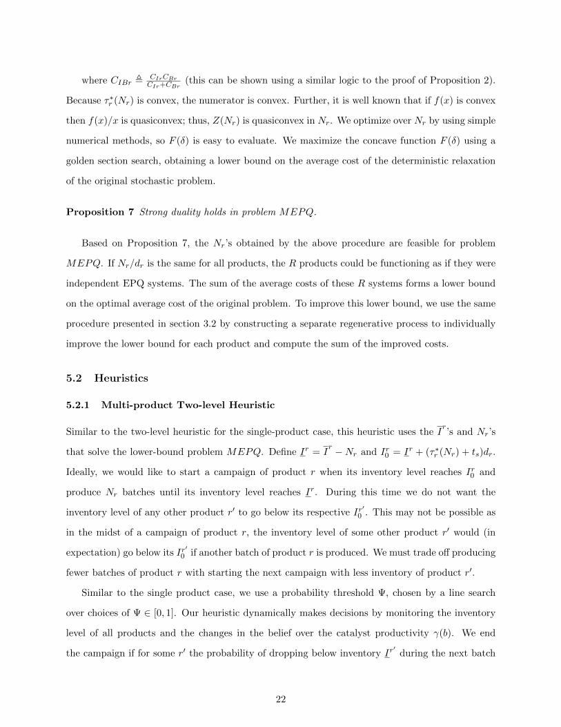
Proposition 7 Strong duality holds in problem MEPQ.

Based on Proposition 7, the Nr’s obtained by the above procedure are feasible for problem

MEPQ. If Nr/dr is the same for all products, the R products could be functioning as if they were

independent EPQ systems. The sum of the average costs of these R systems forms a lower bound

on the optimal average cost of the original problem. To improve this lower bound, we use the same

procedure presented in section 3.2 by constructing a separate regenerative process to individually

improve the lower bound for each product and compute the sum of the improved costs.

5.2 Heuristics

5.2.1 Multi-product Two-level Heuristic

Similar to the two-level heuristic for the single-product case, this heuristic uses the Ir’s and Nr’s

that solve the lower-bound problem MEPQ. Define Ir = Ir −Nr and Ir0 = Ir + (τ∗r (Nr) + ts)dr.

Ideally, we would like to start a campaign of product r when its inventory level reaches Ir0 and

produce Nr batches until its inventory level reaches Ir. During this time we do not want the

inventory level of any other product r′ to go below its respective Ir′

0 . This may not be possible as

in the midst of a campaign of product r, the inventory level of some other product r′ would (in

expectation) go below its Ir′

0 if another batch of product r is produced. We must trade off producing

fewer batches of product r with starting the next campaign with less inventory of product r′.

Similar to the single product case, we use a probability threshold Ψ, chosen by a line search

over choices of Ψ ∈ [0, 1]. Our heuristic dynamically makes decisions by monitoring the inventory

level of all products and the changes in the belief over the catalyst productivity γ(b). We end

the campaign if for some r′ the probability of dropping below inventory Ir′

during the next batch

22

is greater than the threshold. We add a few conditions to ensure that the process is stable (i.e.

inventory does not arbitrarily increase or decrease).

At the end of a campaign, we need to choose the next product rc to produce. For this purpose,

we try to choose the rc that would otherwise induce the largest backlogging cost. Note that

if rc is not produced in the next campaign, it will not be replenished for at least the duration

of the next two campaigns. We approximate the duration of the next two campaigns by τ̂ ,

minr τ∗(N r) + maxr τ

∗(N r), and choose rc as the product with the largest backlogging cost during

this time, starting at its current inventory Ir and ending at Ir − τ̂ dr. With this choice of rc, we

describe the proposed policy for the next campaign.

Let Ir be the inventory level of product r at the end of a campaign, and Irn be the inventory

level of product r after producing batch n in the current campaign. For each product r, define

N rm , arg maxN{N/(τ∗r (N) + ts)}. We split the proposed policy into the following three scenarios,

depending on the inventory vector I after the end of the previous campaign.

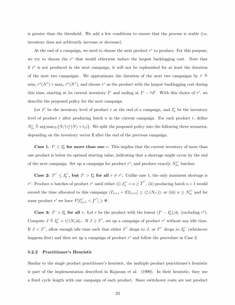
Case 1. Ir ≤ Ir0 for more than one r. This implies that the current inventory of more than

one product is below its optimal starting value, indicating that a shortage might occur by the end

of the next campaign. Set up a campaign for product rc, and produce exactly N rcm batches.

Case 2: Irc ≤ Ir

c

0 , but Ir > Ir0 for all r 6= rc. Unlike case 1, the only imminent shortage is

rc. Produce n batches of product rc until either (i) Irc

n +n ≥ Irc

, (ii) producing batch n+ 1 would

exceed the time allocated to this campaign (Tn+1 + E[tn+1] ≥ τ∗rc(Nrc)), or (iii) n ≥ N rcm and for

some product r′ we have P [Ir′n+1 < Ir

′] ≥ Ψ.

Case 3: Ir > Ir0 for all r. Let r be the product with the lowest (Ir − Ir0)/dr (excluding rc).

Compute J , Ir′

0 + τ∗r (Nr)dr′ . If J ≥ Ir′, set up a campaign of product rc without any idle time.

If J < Ir′, allow enough idle time such that either Ir

′drops to J , or Ir

cdrops to Ir

c

0 (whichever

happens first) and then set up a campaign of product rc and follow the procedure in Case 2.

5.2.2 Practitioner’s Heuristic

Similar to the single product practitioner’s heuristic, the multiple product practitioner’s heuristic

is part of the implementation described in Rajaram et al. (1999). In their heuristic, they use

a fixed cycle length with one campaign of each product. Since switchover costs are not product

23

dependent, the sequence of the products inside the cycle is not considered. Similar to the single

product setting, a fixed batch-operation time t∗r and a target number of batches per campaign Nr

is chosen for each product r. The policy determining when to end a campaign of product r is the

same as in the single-product case. The initial problem solved to determine the cycle length L,

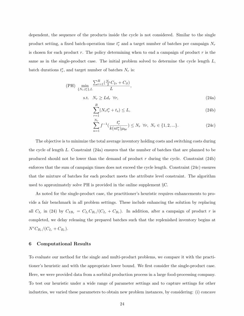
batch durations t∗r , and target number of batches Nr is:

(PH) min{Nr,t∗r},L

∑Rr=1(

Nr2 CIr + CS)

L,

s.t. Nr ≥ Ldr ∀r, (24a)

R∑r=1

(Nrt∗r + ts) ≤ L, (24b)

Nr∑n=1

f−1(t∗r

k(nt∗r)µbr) ≤ Nr ∀r, Nr ∈ {1, 2, ...}. (24c)

The objective is to minimize the total average inventory holding costs and switching costs during

the cycle of length L. Constraint (24a) ensures that the number of batches that are planned to be

produced should not be lower than the demand of product r during the cycle. Constraint (24b)

enforces that the sum of campaign times does not exceed the cycle length. Constraint (24c) ensures

that the mixture of batches for each product meets the attribute level constraint. The algorithm

used to approximately solve PH is provided in the online supplement §C.

As noted for the single-product case, the practitioner’s heuristic requires enhancements to pro-

vide a fair benchmark in all problem settings. These include enhancing the solution by replacing

all CIr in (24) by CIBr = CIrCBr/(CIr + CBr). In addition, after a campaign of product r is

completed, we delay releasing the prepared batches such that the replenished inventory begins at

N rCBr/(CIr + CBr).

6 Computational Results

To evaluate our method for the single and multi-product problems, we compare it with the practi-

tioner’s heuristic and with the appropriate lower bound. We first consider the single-product case.

Here, we were provided data from a sorbital production process in a large food-processing company.

To test our heuristic under a wide range of parameter settings and to capture settings for other

industries, we varied these parameters to obtain new problem instances, by considering: (i) concave

24

k(T ) vs. convex k(T ), (ii) high traffic vs. low traffic, (iii) CB = αCI , α ∈ [0.2, 0.5, 1, 2, 5], and (iv)

low CS , medium CS , high CS .

For concave and convex decay functions, we respectively use kconc(T ) = (1+T )0.7 and kconv(T ) =

12(1 + T )1.2. In all our experiments we use f(q) = − log(q/2).

Define the capacity utilization as the minimum fraction of time that the machine would be busy

(i.e. not idle) to meet demand. In Table 1, low traffic refers to a capacity utilization of 30%, while

high traffic refers to a capacity utilization of 75%. In most problem instances 75% is the highest

capacity utilization for which the practitioner’s heuristic is feasible.

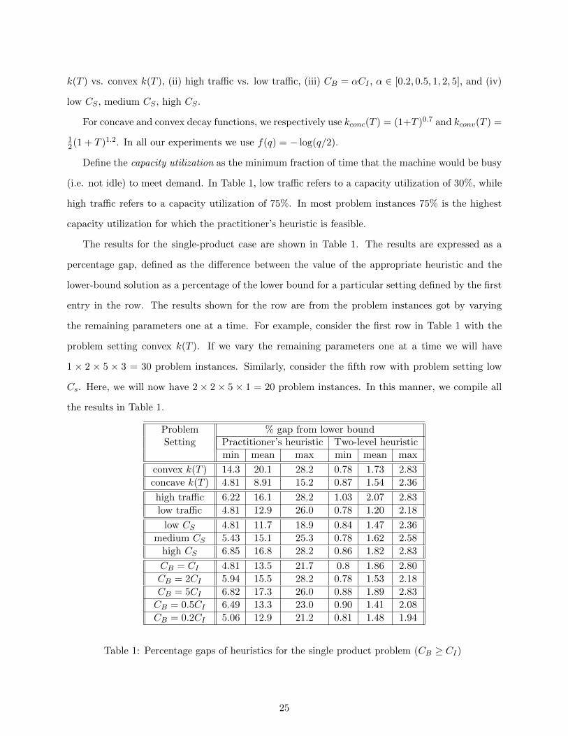
The results for the single-product case are shown in Table 1. The results are expressed as a

percentage gap, defined as the difference between the value of the appropriate heuristic and the

lower-bound solution as a percentage of the lower bound for a particular setting defined by the first

entry in the row. The results shown for the row are from the problem instances got by varying

the remaining parameters one at a time. For example, consider the first row in Table 1 with the

problem setting convex k(T ). If we vary the remaining parameters one at a time we will have

1 × 2 × 5 × 3 = 30 problem instances. Similarly, consider the fifth row with problem setting low

Cs. Here, we will now have 2 × 2 × 5 × 1 = 20 problem instances. In this manner, we compile all

the results in Table 1.

Problem % gap from lower boundSetting Practitioner’s heuristic Two-level heuristic

min mean max min mean max

convex k(T ) 14.3 20.1 28.2 0.78 1.73 2.83

concave k(T ) 4.81 8.91 15.2 0.87 1.54 2.36

high traffic 6.22 16.1 28.2 1.03 2.07 2.83

low traffic 4.81 12.9 26.0 0.78 1.20 2.18

low CS 4.81 11.7 18.9 0.84 1.47 2.36

medium CS 5.43 15.1 25.3 0.78 1.62 2.58

high CS 6.85 16.8 28.2 0.86 1.82 2.83

CB = CI 4.81 13.5 21.7 0.8 1.86 2.80

CB = 2CI 5.94 15.5 28.2 0.78 1.53 2.18

CB = 5CI 6.82 17.3 26.0 0.88 1.89 2.83

CB = 0.5CI 6.49 13.3 23.0 0.90 1.41 2.08

CB = 0.2CI 5.06 12.9 21.2 0.81 1.48 1.94

Table 1: Percentage gaps of heuristics for the single product problem (CB ≥ CI)

25

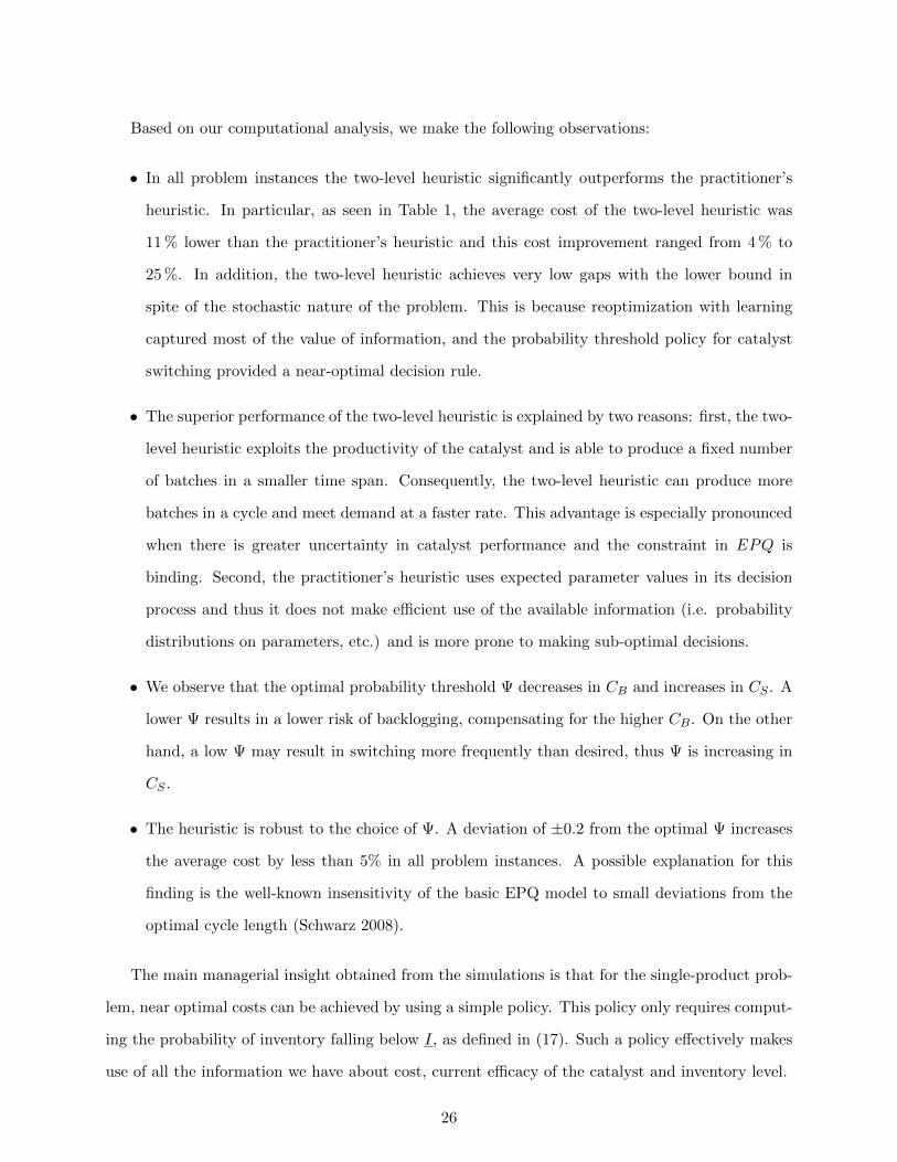
Based on our computational analysis, we make the following observations:

• In all problem instances the two-level heuristic significantly outperforms the practitioner’s

heuristic. In particular, as seen in Table 1, the average cost of the two-level heuristic was

11 % lower than the practitioner’s heuristic and this cost improvement ranged from 4 % to

25 %. In addition, the two-level heuristic achieves very low gaps with the lower bound in

spite of the stochastic nature of the problem. This is because reoptimization with learning

captured most of the value of information, and the probability threshold policy for catalyst

switching provided a near-optimal decision rule.

• The superior performance of the two-level heuristic is explained by two reasons: first, the two-

level heuristic exploits the productivity of the catalyst and is able to produce a fixed number

of batches in a smaller time span. Consequently, the two-level heuristic can produce more

batches in a cycle and meet demand at a faster rate. This advantage is especially pronounced

when there is greater uncertainty in catalyst performance and the constraint in EPQ is

binding. Second, the practitioner’s heuristic uses expected parameter values in its decision

process and thus it does not make efficient use of the available information (i.e. probability

distributions on parameters, etc.) and is more prone to making sub-optimal decisions.

• We observe that the optimal probability threshold Ψ decreases in CB and increases in CS . A

lower Ψ results in a lower risk of backlogging, compensating for the higher CB. On the other

hand, a low Ψ may result in switching more frequently than desired, thus Ψ is increasing in

CS .

• The heuristic is robust to the choice of Ψ. A deviation of ±0.2 from the optimal Ψ increases

the average cost by less than 5% in all problem instances. A possible explanation for this

finding is the well-known insensitivity of the basic EPQ model to small deviations from the

optimal cycle length (Schwarz 2008).

The main managerial insight obtained from the simulations is that for the single-product prob-

lem, near optimal costs can be achieved by using a simple policy. This policy only requires comput-

ing the probability of inventory falling below I, as defined in (17). Such a policy effectively makes

use of all the information we have about cost, current efficacy of the catalyst and inventory level.

26

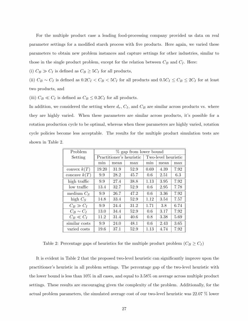
For the multiple product case a leading food-processing company provided us data on real

parameter settings for a modified starch process with five products. Here again, we varied these

parameters to obtain new problem instances and capture settings for other industries, similar to

those in the single product problem, except for the relation between CB and CI . Here:

(i) CB � CI is defined as CB ≥ 5CI for all products,

(ii) CB ∼ CI is defined as 0.2CI < CB < 5CI for all products and 0.5CI ≤ CB ≤ 2CI for at least

two products, and

(iii) CB � CI is defined as CB ≤ 0.2CI for all products.

In addition, we considered the setting where dr, CI , and CB are similar across products vs. where

they are highly varied. When these parameters are similar across products, it’s possible for a

rotation production cycle to be optimal, whereas when these parameters are highly varied, rotation

cycle policies become less acceptable. The results for the multiple product simulation tests are

shown in Table 2.

Problem % gap from lower boundSetting Practitioner’s heuristic Two-level heuristic

min mean max min mean max

convex k(T ) 19.20 31.9 52.9 0.69 4.39 7.92

concave k(T ) 9.9 28.2 45.7 0.6 2.51 6.3

high traffic 9.9 27.4 38.8 1.13 3.95 7.92

low traffic 13.4 32.7 52.9 0.6 2.95 7.78

medium CS 9.9 26.7 47.2 0.6 3.36 7.92

high CS 14.8 33.4 52.9 1.12 3.54 7.57

CB � CI 9.9 24.4 31.2 1.71 3.8 6.74

CB ∼ CI 13.0 34.4 52.9 0.6 3.17 7.92

CB � CI 11.2 31.4 40.6 0.8 3.38 5.69

similar costs 9.9 24.0 48.1 0.6 2.43 3.65

varied costs 19.6 37.1 52.9 1.13 4.74 7.92

Table 2: Percentage gaps of heuristics for the multiple product problem (CB ≥ CI)

It is evident in Table 2 that the proposed two-level heuristic can significantly improve upon the

practitioner’s heuristic in all problem settings. The percentage gap of the two-level heuristic with

the lower bound is less than 10% in all cases, and equal to 3.58% on average across multiple product

settings. These results are encouraging given the complexity of the problem. Additionally, for the

actual problem parameters, the simulated average cost of our two-level heuristic was 22.07 % lower

27

than the practitioner’s heuristic. Thus, this approach if used, has the potential to significantly

reduce operational costs. The following additional observations can be drawn from the multi-

product case:

• Under the practitioner’s heuristic, the average cost of operation is significantly higher when

the cost and demand parameters are varied across products relative to when the parameters

are similar across products. This is because the practitioner’s heuristic uses a rotation cycle

in which the cycle length of all the products are the same. As the product parameters

become more diverse, it becomes less sensible to have the same cycle length for all products.

In contrast, the two-level heuristic is a dynamic policy designed specifically to take such

variation in product parameters into account. However, even with the two-level heuristic,

costs are slightly higher when products are more diverse because it becomes harder to reach

a stable production pattern. Nevertheless, the gaps of the two-level heuristic with the lower

bound are quite low for all problem settings.

• Similar to the single product case, the percentage gaps of the practitioner’s heuristic signif-

icantly increase when CS is high. However, the two-level heuristic performs well because it

dynamically controls all products to follow their optimal EPQ cycles as closely as possible.

The EPQ cycle trades off CS with CI and CB and it is robust to changes in the “production

quantity”, which explains why slight deviations do not significantly increase the average costs

as long as a good policy is in place to make the switching decisions.

The following managerial insights can be drawn from the computational analysis. These could

also be useful for practitioners in similar industries:

1. Our relatively simple two-level heuristic nearly attains the optimal cost of the intractable

stochastic decision process. The optimal cost is closely approximated by our simulation-based

stochastic lower bound.

2. For minimizing the duration of a campaign of a fixed number of batches, the value of in-

formation, Bayesian learning, and dynamic decision making can be adequately captured by

employing a re-optimization policy in conjunction with observing and learning.

28

3. When deciding on the next product to produce, we can choose the product with the greatest

expected backlogging cost during the next two campaigns. This is somewhat similar to

employing a one-step look-ahead policy, and our numerical results support its effectiveness.

4. When deciding whether or not to switch, the probability that the inventory of each product

r falls below its respective threshold Ir provides an efficient summary of the intractable

multidimensional state of the system. This can be used to make the important decision of

when to change the catalyst and switch to the next campaign.

Note that our methods still require repeated Bayesian updating of the belief distribution on

the catalyst parameter (this is needed for more accurate computations of E[tn+1] and P [In+1 <

I]). However, such mathematical procedures seem amenable to implementation, given the ready

availability of data from the process control system and tools from standard commercially available

statistical software.

7 Conclusions

The problem of production campaign planning with uncertainty in production times, learning

about production characteristics, and decay in catalyst performance is a challenging but important

problem in a variety of process industry sectors such as food processing, pharmaceuticals, and

specialty chemicals. We first considered the single product case and formulated it as an SMDP. To

solve this problem, we developed a two-level heuristic. This heuristic splits the problem into a batch-

planning problem and a catalyst-switching policy. The batch planning problem determines the

production duration of each batch, given the fact that the quality of future batches depends on the

decision made on earlier batches. Catalyst-switching defines a policy of when to stop the campaign

and switch the catalyst. We present a practitioner’s heuristic, used at a large food-processing

company, to benchmark the two-level heuristic. To assess the quality of this heuristic, we develop

a lower bound to the SMDP by associating this process with another stochastic process with an

infinitely recurrent state. The proposed framework of associating a continuous state space dynamic

programming problem with a similar but regenerative process is applicable to other stochastic

dynamic programming problems. We then considered the multiple product case. We modeled

the relaxed deterministic approximation as a constrained economic lot sizing model, and used a

29

Lagrange relaxation to solve it. We were able to directly extend all the results and techniques of

the single product problem to the multiple product setting.

The computational results for the single and multiple product problems show that our heuristics

achieve low percentage gaps with the lower bound on the optimal average costs. In addition,

our approach significantly outperforms the practitioner’s heuristic currently employed by a leading

food-processing company. Furthermore, our heuristics are robust to changes in the cost parameters.

This allows us to further simplify the proposed dynamic policy and present general and easy to

implement operational guidelines for practitioners.

This paper opens up several avenues for future research. First, our model could be extended

to the case with multiple reactors. Second, one could consider alternate quality models that may

be required for meeting attribute quality levels. Third, these techniques could be applied to other

industries that would require incorporating different types of production constraints. All these

extensions might require significant modifications to the methods presented in this paper and could

be fruitful areas for future work.

References

Brown, D. B., & Smith, J. E. (2013). Optimal sequential exploration: Bandits, clairvoyants, and

wildcats. Operations research, 61(3), 644-665.

Casas-Liza, J., Pinto, J. M., & Papageorgiou, L. G. (2005). Mixed integer optimization for cyclic

scheduling of multiproduct plants under exponential performance decay. Chemical Engineering

Research and Design, 83(10), 1208–1217.

Ciocan, D. F., & Farias, V. (2012). Model predictive control for dynamic resource allocation.

Mathematics of Operations Research, 37(3), 501-525.

Levi R., Shi C., 2013. Approximation Algorithms for the Stochastic Lot-Sizing Problem with Order

Lead Times. Operations Research 61(3), 593–602.

Liu, S., Yahia, A., & Papageorgiou, L. G. (2014). Optimal Production and Maintenance Plan-

ning of Biopharmaceutical Manufacturing under Performance Decay. Industrial & Engineering

Chemistry Research, 53(44), 17075-17091.

Loehndorf, N., & Minner, S. (2013). Simulation optimization for the stochastic economic lot

scheduling problem. IIE Transactions, 45(7), 796-810.

Mazzola J. B., McCardle K. F., 1996. A Bayesian approach to managing learning curve uncertainty.

Management Science 42(5), 680–692.

30

Rajaram, K., Jaikumar, R. (posthumously), Behlau, F., van Esch, F., Heynen, C., Kaiser, R.,

Kuttner, A. and van de Wege, I. (1999). Robust Process Control at Cerestars Refineries.

Interfaces, Special Issue: Franz Edelmann Award Papers, 29(1), 30-48.

Rajaram K., & Karmarkar U.S., (2002). Product Cycling With Uncertain Yields: Analysis And

Application To The Process Industry. Operations Research 50(4), 680–691.

Rajaram, K., & Karmarkar, U. S. (2004). Campaign planning and scheduling for multiproduct

batch operations with applications to the food-processing industry. Manufacturing & Service

Operations Management, 6(3), 253-269.

Schwarz, L. B. (2008). The economic order-quantity (EOQ) model. In Building Intuition (pp.

135-154). Springer US.

Vaughan, T. S. (2007). Cyclical schedules vs. dynamic sequencing: Replenishment dynamics and

inventory efficiency. International Journal of Production Economics, 107(2), 518-527.

Wang, J., Li, X., & Zhu, X. (2012). Intelligent dynamic control of stochastic economic lot scheduling

by agent-based reinforcement learning. International Journal of Production Research, 50(16),

4381-4395.

Winands, E. M., Adan, I. J., & Van Houtum, G. J. (2011). The stochastic economic lot scheduling

problem: A survey. European Journal of Operational Research, 210(1), 1–9.

Appendix: Stochastic Lower Bound Algorithm

We refer to the original process as a “Type A” process and to the regenerative process as a

“Type B” process. This simulation based algorithm is designed to compute a lower bound on the

minimum average cost of a type B process given I∗0 .

1. Set λ to λEPQ (the optimal cost of problem (11)).

2. Repeat the following simulation procedure until the simulated average cost seems to have

converged:

set up a campaign at inventory level I∗0 . Simulate a b and a sequence of zis, then with full

information on the outcome of b and z, plan the campaign to minimize the differential cost

of the current cycle. The decision variables are the number of batches N and the attribute

levels qi, summarized in the vector q. Let I(q) , I∗0 − τ(q, b, z)d denote the inventory level

after the campaign. The differential cost of the cycle is evaluated as follows:

31

(i) If I(q) +N ≤ I∗0 , the differential cost is:

g(I∗0 , tI0I(q))− λtI0I(q) − g(I∗0 , tI0I′) + λEPQtI0I′

where tI0I(q) = (I∗0 − I(q))/d is the time required for inventory to go from I∗0 to I(q). The

term −g(I∗0 , tI0I′) + λEPQtI0I′ is the cost of instantly raising the inventory level from I(q) to

I∗0 , from the definition of a type B process, and tI0I′ = (I0 − I(q)−N)/d.

(ii) If I(q) +N ≥ I∗0 , the differential cost is:

g(I∗0 , tI0I(q))− λtI0I(q) + minI∗0≤I≤I(q)+N

{g(I, tII0)− λtII0}

where the term min{g(I, tII0) − λtII0} comes from the definition of process B. It allows the

inventory to drop instantly from I(q) + N to any I such that I∗0 ≤ I ≤ I(q) + N . In the

optimal policy for process B, the chosen I is one that minimizes the differential cost to return

to I∗0 . It is easy to check that the differential cost increases with N after I(q∗) + N < 0.

Hence, the largest N that needs to be considered is the first N that satisfies I(q∗) +N < 0.

Once q is chosen, record the cycle cost and cycle time (respectively equal to g(I∗0 , tI0I(q)) −

g(I∗0 , tI0I′)+λEPQtI0I′ and tI0I(q) for case (i), and equal to g(I∗0 , tI0I(q))+min{g(I, tII0)−λtII0}

and λtI0I(q) for case (ii)) to enable computing of the average total cost after each iteration

and checking for convergence.

3. Update the value of λ to the average cost computed in step 2, and return to step 2. Repeat

this process until λ converges. The resulting λ is the optimal cost of a type B process.

To prove that this algorithm converges to a lower bound, note that the simulated process is an

analog of process B, where the decisions are made with full information on b and z. Therefore the

optimal cost of this process is a lower bound on the optimal cost of process B. Additionally, this

process is also regenerative, as the inventory level I∗0 before campaign setup is a recurrent state,

hence the value iteration algorithm converges to the optimal cost (Bertsekas (1995, vol. 2)). This

algorithm is also effectively a value iteration algorithm, where the λ at each iteration is evaluated

using simulation.

32

Production Campaign Planning Under Learning and DecayOnline Supplement

A Proof of Propositions

Proposition 1. To prove that the constrained EPQ (11) provides a lower bound on the original

SMDP (7), we show that a feasible solution to (11) exists with equal or less cost than the optimal

average cost of the original process.

A cycle is defined from the end of one campaign to the end of the next campaign and includes

any idle time. The average total costs of inventory holding, backlogging, and catalyst switching

can be re-written as:

λ = limT→∞

∫ T0 (I(w)+CI + I(w)−CB + δs(w)Cs)dw

T= I

+θ+CI + I

−θ−CB +

CS

Tcyc(1)

where I(w) is the inventory level at time w, I(w)+ , max[0, I(w)], and I(w)− , max[0,−I(w)].

The function δs(w) has a unit impulse at every time w where a switching occurs, and is zero for all

other w. Further simplification results in the righthand side of (1), where I+

(I−

) is the inventory

level averaged over all instances where I(w) ≥ 0 (I(w) < 0), and θ+ (θ−) is the fraction of total

time where I(w) ≥ 0 (I(w) < 0), and Tcyc is the average cycle time.

Let the superscript ∗ represent the optimal production strategy. We show that a fixed cycle

strategy (following the EPQ formulation (11)) exists for which the optimal average cost is equal

to or less than λ∗ = I+∗θ+∗CI + I

−∗θ−∗CB + CS

Tcyc∗ . For this fixed cycle strategy, let θ+ = θ+

∗,

θ− = θ−∗, and Tcyc = Tcyc

∗; i.e. the cycle always starts from inventory Tcyc

∗θ+∗d and finishes at

inventory −Tcyc∗θ−∗d, and a total of Tcyc

∗d batches are produced in each campaign. The feasibility

of the cycle length Tcyc∗

in the deterministic constraint of problem (11) (i.e. τ∗(Tcycd) + ts ≤ Tcyc)

follows from the convexity of τ∗(N), Jenson’s inequality, and the fact that τ∗(N) is a lower bound

on the expected campaign length for N batches. It suffices to show that for this fixed cycle strategy

I+ ≤ I+

∗and I

− ≤ I−∗.

For the optimal production strategy, assume a total of M cycles and let M → ∞. The total

production time is MTcyc∗

and the total time spent in negative inventory levels is θ−∗MTcyc

∗. Let

the number of cycles that reach negative inventory be M ′ ≤ M . Hence the average time spent in

1

negative inventory levels per negative turn is:

T− , limM→∞

θ−∗MTcyc

∗

M ′≥ θ−∗Tcyc (2)

Assume that in the optimal strategy, all cycles start with a positive inventory level (the proofs

for alternative cases follow with similar reasoning). The average negative inventory level per neg-

ative turn is T−d2 . This is not the average inventory level over the total time span of negative

inventory; rather it is the average over the number of cycles that reach negative values. To obtain

the per-time average, we must compute a weighted average over the cycles: the average negative

inventory level of each cycle must be weighted proportional to the total amount of time that specific

cycle spends in negative inventory. Notice that in this case, the cycles that reach larger (absolute)

negative inventory levels will be weighted more heavily (because they must spend a longer time in

negative inventory to reach that level) and cycles that end at smaller (absolute) negative inventory

levels will be weighted less. The resulting I−∗

will be greater than T−d2 and thus I

−∗ ≥ θ−∗Tcycd2 .

Notice that for the fixed cycle strategy previously defined, I−

=θ−

∗Tcycd2 . Hence, I

− ≤ I−∗

. It

follows with similar reasoning that I+ ≤ I+

∗, which completes the proof �

Proposition 2. Let a , I/Tcycd denote the proportion of Tcyc where the inventory level is

positive. The maximum inventory during Tcyc is aTcycd and the average is aTcycd/2. The proportion

of Tcyc where the inventory is negative is 1− a, with a maximum of (1− a)Tcycd and an average of

(1− a)Tcycd/2 during this time. Hence, the average cost during the cycle time Tcyc becomes:

Cs + (aTcyc)(aTcycd/2)CI + [(1− a)Tcyc][(1− a)Tcycd/2]CBTcyc.

Minimizing with respect to a gives a∗ = CBCI+CB

. Substituting for a and arranging the terms, the

objective function becomes

CsTcyc

+

(CICBCI + CB

)Tcycd

2,

which is a convex function of Tcyc �

Proposition 3. We prove the existence of I = argmin{w(I)}, where w(I) was defined in (7).

2

Observe that

(i) w(I) grows unboundedly as I → ±∞, and

(ii) w(I) is bounded below.

To prove that w(I) is bounded below, assume that for some I = I−∞ we have w(I−∞) = −∞.

Because we assume that the highest achievable average production rate exceeds the demand rate,

we are able to reach I−∞ from any initial state with probability 1 in finite time by producing at the

highest rate until inventory goes over I−∞, then allowing idle time until inventory drops to I−∞.

For all states I we would have w(I) = −∞, which is a contradiction �

Proposition 4. If the process reaches state I∗

and production has stopped (the next campaign

has not yet been set up), the only state variable determining the decision will be the inventory

level I∗. The optimal decision is either to set up the next campaign immediately (in which case

I∗0 = I∗) or to idle the process until the inventory level reaches a certain value which we call I∗0 . I∗0

is constant because the decision at inventory level I∗

when the process is idle is independent of the

history of the process �

Proposition 5. For the purpose of this proof, we refer to the original process as a “Type

A” process and to the regenerative process as a “Type B” process. Define a process of type B

that during a campaign, follows the same batch planning and catalyst switching decisions as in

the optimal policy of process A. Once the campaign is ended, if the inventory I after a campaign

is below I∗0 , raise it instantly to I∗0 at a cost of −g(I∗0 , tI0I) + λEPQtI0I . If I∗0 ≤ I ≤ I∗, idle the

process till it reaches inventory I∗0 and then set up the next campaign. If I > I∗, instantly decrease

I to I∗

and idle the process till it reaches I∗0 . We show that the process B defined here has a lower

average cost than the optimal process A.

Let w∗ denote the differential costs of the optimal policy of process A (as defined in (7)), and let

λ∗ be the optimal cost of process A.

(i) Assume that in the optimal process A, inventory level reaches I ≤ I∗0 after a campaign.

Noting that the optimal policy would not idle the process from I∗0 to I (by the definition of I∗0 ), we

3

have:

w∗(I∗0 ) ≤ g(I∗0 , tI0I) + w∗(I)− λ∗tI0I

⇒w∗(I) ≥ w∗(I∗0 )− g(I∗0 , tI0I) + λ∗tI0I

⇒w∗(I) ≥ w∗(I∗0 )− g(I∗0 , tI0I) + λEPQtI0I

where the last inequality follows from the fact that λEPQ is a lower bound to the optimal cost. The

left-side of this inequality is the optimal ongoing differential cost of process A and the right side is

the ongoing differential cost of the defined type B process.

(ii) Alternatively assume that I > I∗0 . If I ≤ I∗, then the optimal decision in process A is to

idle the process to reach inventory level I∗0 and set up the next campaign at I∗0 , same as in the

defined process B. If I > I∗, then by definition of I

∗we know that w∗(I) ≥ w∗(I∗). Since the type

B process instantly decreases from I to I∗, its ongoing differential cost will be less than or equal

to that of process A.

Hence, regardless of where the process begins, the ongoing differential cost of the defined process

B is less than or equal to that of the optimal process of type A �

Proposition 6. The objective is to minimize Eb[τ(q, b)] over q of known length N . For

i ∈ {2, 3, ..., N}, let Q∗i+1 be the value in the optimal q. Note that Q∗N+1 = N . Define R as the

total attribute level that must be met by qi and qi−1.

R , Q∗i+1 −Q∗i−1 = qi + qi−1. (3)

The optimal allocation of R between qi and qi−1 solves:

min ψ(qi−1, qi) = Eb,z1,z2 [(b+ z1)f(qi−1)k(Ti−1) + (b+ z2)f(qi)k(Ti)]

s.t. qi + qi−1 = R

Ti = Ti−1 + (b+ zi)f(qi−1)k(Ti−1).

(4)

For notational simplicity let bi , b + zi (which implies Ezi(bi) = b). Let q > q′ > 0 such that

q + q′ = R, and let ∆T , b1k(T )f(q) and ∆T ′ , b1k(T )f(q′); then ∆T ′ > ∆T . For any b ≥ 0 we

4

have:

ψ(q, q′) ≤ ψ(q′, q)

⇔Ez[b1k(T )f(q) + b2k(T + b1k(T )f(q))f(q′)] ≤ Ez[b1k(T )f(q′) + b2k(T + b1k(T )f(q′))f(q)]

⇔bf(q′)(Eb1 [k(T + ∆T )]− k(T )) ≤ bf(q)(Eb1 [k(T + ∆T ′)]− k(T ))

⇔Eb1 [k(T + ∆T )]− k(T )

bf(q)≤ Eb1 [k(T + ∆T ′)]− k(T )

bf(q′)(5)

Convexity of k(T ) is sufficient for the last inequality to hold, because

∆T ′ > ∆T and k(T ) is convex⇒ k(T + ∆T )− k(T )

∆T≤ k(T + ∆T ′)− k(T )

∆T ′∀ b1 ≥ 0

⇒ k(T + ∆T )− k(T )

b1k(T )f(q)≤ k(T + ∆T ′)− k(T )

b1k(T )f(q′)∀ b1 ≥ 0

⇒ k(T + ∆T )− k(T )

bf(q)≤ k(T + ∆T ′)− k(T )

bf(q′)∀ b1 ≥ 0

⇒ Eb1 [k(T + ∆T )]− k(T )

bf(q)≤ Eb1 [k(T + ∆T ′)]− k(T )

bf(q′)

(6)

Hence

k(T ) convex and q > q′ ⇒ ψ(q, q′) ≤ ψ(q′, q) (7)

Assume that in the optimal solution to (4) for convex k(T ), qi−1 > qi. Then there exists an

equally good or better solution by exchanging qi−1 and qi. Hence if k(T ) is convex, there is always

an optimal solution in which qi−1 ≤ qi. If k(T ) is strictly convex, the inequalities in (5) become

strict inequalities, which proves there are no optimal solutions where qi−1 > qi. This proves part

(i).

Similarly, for concave k(T ), the direction of the inequalities in (5) are reversed which proves

part (ii). Part (iii) is straightforward: replace k(T ) by a+ cT and take the derivative w.r.t. q �

Proposition 7. By using a change of variables N−1r = 1/Nr, we obtain a convex optimization

problem over the variables N−1r (note that if f(x) is convex, then xf(x−1) is convex over positive

values of x). The convex set defined by the constraint has an interior point because the maximum

achievable production rate is strictly greater than the demand rate. Hence Slater’s condition holds

for the problem over N−1r and strong duality holds. The solutions to the primal and dual problems

5

are unaffected by the change of variables from Nr to N−1r , hence strong duality also holds for the

original problem (20) over Nr �

B 3-Batch Example for Sufficiency of Re-optimization Policy

We consider a 3-batch campaign (N = 3) and sequentiall choose q1, q2, and q3 to minimize the

total duration of the campaign. We consider two planning scenarios: in the first scenario, a policy

q = [q1, q2, q3] is computed as q = arg minqEb,z{τ(q, b, z)}, of which q1 is executed, then [q2, q3]

is re-optimized after observing t1. In the second scenario, q1, q2, and q3 are sequentially chosen

as the optimal solutions to the dynamic program (15). In the first scenario, in choosing q1 we

do not anticipate the fact that we are able to choose [q2, q3] based on more accurate information,

whereas in the second scenario we solve a dynamic program that accounts for all outcomes of t1. To

evaluate the most extreme-case difference between the two scenarios and to enable tractability of

the dynamic program, we assume that full information becomes available once we observe t1. That

is, we assume that b is initially unknown, but is learned through f−1(t1/k(0)) once t1 is observed

(there are no random shocks to hinder the learning process). With these settings, the dynamic

program (15) converts to a two-stage formulation as follows:

v2(q1, t1) = minq2

[bk(t1)f(qi) + bk(t1 + t2)f(3− q1 − q2)],

where b = f−1(t1/k(0)) and t2 = bk(t1)f(qi),

v1(0, 0) = minq1

[Eb{bk(0)f(q1) + v2(q1, bk(0)f(q1))}].

(8)

A numerical solution to (8) is computed by discretizing and enumerating q1, q2, and b, which

evaluates the expected campaign length under scenario 2 and also allows computing q∗1. The first

scenario is also evaluated by enumerating q1, q2, and b, but here instead of q1 being the optimal

solution to (8), it is the first element in q = arg minqEb{τ(q, b)} (denoted by qs1). Additionally,

the expected optimal campaign duration under apriori knowledge of b (i.e. a clairvoyant decision

maker) is evaluated using Eb{minq[τ(q, b)]} (also using enumeration).

We may now compare the two policies by computational experiments. We let f(q) = − log(q/2),

and in order to compare the policies under a wide range of settings, we consider three classes of

functions for the catalyst decay function k(T ):

6

(i) k(T ) = a(T + 1)p,

(ii) k(T ) = a log(T + 2),

(iii) k(T ) = a exp(T ).

For class (i), we alter the scale parameter a within the range [0.1, 100] and the power parameter

p within the range [0.2, 3]. For classes (ii) and (iii), we alter the scale parameter a within the ranges

[1, 100] and [0.1, 2] respectively. In all our test problems, we assume a normal prior on b with mean

1 and standard deviation 0.2. We consider 220 problem settings in total, and make the following

observations, which are also summarized in §4.1 and used to justify the re-optimization policy.

1. Considering the fact that we enumerate q1 in increments of 0.02 in the range [0.02, 2], q∗1

and qs1 coincide in 209 out of 220 problem instances, and have at most 0.04 difference in the

remaining 11 instances.

2. In all 220 problem instances the expected campaign time under the re-optimization policy is

within 1% of the expected campaign time under the optimal policy.

3. In all 220 problem instances the expected campaign time under both policies is within 2% of

the expected optimal campaign time under apriori knowledge of b.

C Algorithm for solving PH

In the practitioner’s heuristic for the multi-product case, the problem PH is approximately solved

by iterating over t∗r of one product. Choose any one of the R products and index it by r̂.

Algorithm.

1. Initiate t̂ = t0 and δ := step size.

2. Let t∗r̂ = t̂.

3. Let Nr̂ = max[N ] s.t.∑N

n=1 f−1(

t∗r̂k(nt∗r̂)µbr̂

) ≤ N .

4. Let L = Nr̂/dr̂.

5. Let Nr = dLdre for all other r.

6. Let t∗r = min[tr] s.t.∑N

n=1 f−1( t∗r

k(nt∗r)µbr) ≤ Nr for r 6= r̂.

7. If the variables chosen in steps 2-6 meet the constraints (24a)-(24c), evaluate t̂ by V (t̂) =∑Rr=1(

Nr2CIr+CS)

L . Otherwise, V (t̂) =∞.

8. t̂+ δ → t̂. If t̂ > 1dr, go to 9; otherwise go to 2.

7

9. Let t∗r̂ = arg minV (t̂), choose the rest of the variables by the procedure in steps 3-6, and termi-

nate.

To understand the assignments in steps 4 and 5 of the Algorithm, observe that in the optimal

solution to PH, the equations L = min Nrdr

and Nr = dLdre will hold: if L < min Nrdr

, L can increase

without violating the constraints, reducing the objective function. If Nr > dLdre, Nr can decrease

to reduce the objective function. Both cases contradict optimality. Therefore, the assignment in

steps 4 and 5 satisfies the mentioned equations.

8