PRODUCTION AND OPERATIONS MANAGEMENTaatasu3/index_files/AC06.pdf · PRODUCTION AND OPERATIONS MANAGEMENT POMS Vol. 15, No. 4, Winter 2006, pp. 473–487 ... 474 Production and Operations

Lot Sizing for Optimal Collection and Useof Remanufacturable Returns over a

Finite Life-Cycle

Atalay Atasu • Sıla CetinkayaINSEAD, Boulevard de Constance, 77300 France

Industrial & Systems Engineering, Texas A&M University, College Station, Texas 77843-3131, [email protected] • [email protected]

Reverse supply chains process used product returns to recover value by re-processing them viaremanufacturing operations. When remanufacturing is feasible, the longer the return flows are

delayed during the active (primary) market demand period of the product, the lower the value that canbe recovered through these operations. In fact, in order to recover the highest value from remanufac-tured products, the collection rates, return timings, and reusability rates should be matched with theactive market demand and supply. With these motivations, this paper is aimed at developing analyticalmodels for the efficient use of returns in making production, inventory, and remanufacturing decisionsduring the active market. More specifically, we consider a stylistic setting where a collector collects usedproduct returns and ships them to the manufacturer who, in turn, recovers value by remanufacturingand supplies products during the active market demand. Naturally, the manufacturer’s production,inventory and remanufacturing decisions and costs are influenced by the timing and quantity of thecollector’s shipments of used product returns. Hence, we investigate the impact of the timing of returnson the profitability of the manufacturer-collector pair by developing system-wide cost optimizationmodels. Analyzing the properties of the optimal shipment frequency, we observe that the fastest reversesupply chain may not always be the most efficient one.

Key words: product returns; remanufacturing; inventory control; life cycleSubmissions and Acceptance: Received January 2005; revisions received August 2005 and November 2005;

accepted December 2005.

1. IntroductionThis paper concentrates on inventory optimization fornew and remanufactured products in a setting wherethe remanufactured products are perfectly substitut-able for the new products during the period of activemarket demand. We use the terms “returns” and“used product returns” interchangeably for returnedproducts before remanufacturing. We use the term“remanufactured products” for returned products af-ter remanufacturing. The focus of the paper is on finitelife cycle settings, and, hence, the term active marketdemand refers to the demand from the beginning untilthe end of the corresponding life cycle. The specificproducts of interest are from the refillable containermanufacturing/remanufacturing industry. Well-knownexamples of such products include single-use cameras

and copy/print cartridges (Guide and Wassenhove2004) for which a finite life cycle setting, with perfectsubstitution of new and remanufactured products, isrepresentative of practice. As noted by Guide and VanWassenhove (2004), refillable container remanufactur-ing is one of the older forms of returned product usewhere the returns come directly from the consumer.Kodak and Xerox implement two current examples ofthis practice; both companies’ customers take usedproduct returns (single-use camera and cartridge, re-spectively) to a collection location, and the returns arethen remanufactured and distributed through normaldistribution channels. The remanufactured productsare not distinguishable from new products, and theunit remanufacturing cost is less than the unit cost ofa new product, so remanufacturing is a potentially

POMSPRODUCTION AND OPERATIONS MANAGEMENTVol. 15, No. 4, Winter 2006, pp. 473–487issn 1059-1478 � 06 � 1504 � 473$1.25 © 2006 Production and Operations Management Society

473

economical option. In this setting, the longer the re-turn flows are delayed during the active market de-mand period of the product, the lower the value thatis recovered through remanufacturing.

In fact, for recovering the highest value from re-manufactured products, the return timing, as well asthe collection and reusability rates, should be matchedwith the active market demand and supply. Recogniz-ing this fact, the current paper develops analyticalmodels for the efficient use of returns in making pro-duction, inventory, and remanufacturing lot-size de-cisions during the period of active market demand.More specifically, we consider a stylistic setting wherea collector collects used product returns and shipsthem to the manufacturer who, in turn, recovers valuethrough remanufacturing operations and supplyingthe remanufactured products during the active marketdemand period. The collector incurs a holding costuntil a shipment is released to the manufacturer at afixed shipment cost, and, hence, he/she is interestedin balancing these two costs. The manufacturer is themajor supplier for the market demand, and, naturally,his/her production, inventory, and remanufacturingdecisions, e.g., his/her lot-sizing related decisions, areinfluenced by the timing and quantity of the collector’sshipments of used product returns. The basic issue weinvestigate is the impact of the timing of used productreturn shipments from the collector to the manufac-turer on the system-wide cost of the manufacturer-collector pair so that we can demonstrate the value ofcoordinating production, return, and demand flows,and, hence, the time value of returns, in a simple settingunder centralized control. To this end, we developsystem-wide cost optimization models for the purposeof computing the optimal timing of return shipmentsfrom the collector to the manufacturer. Consequently,these models seek to identify production, inventory,and remanufacturing policies that are aimed at theefficient use of remanufactured products during the periodof active market demand. In addition, by analyzing theproperties of the optimal shipment frequency, we ob-serve that the fastest reverse supply chain may notalways be the most efficient one.

To summarize, while emphasizing on the fact thattiming is critical under finite life cycles, our analyticalwork is aimed at answering the following questions:

• What are the impacts on the reverse logistics sys-tem of (i) the length of a finite life cycle, (ii) theamount of time used product returns stay withthe original customers, and (iii) the amount oftime used product returns stay at the collectionfacility?

• What are the impacts of (i) to (iii) on the timevalue of returns?

• Under what conditions should the reverse logis-tics system be faster?

• How would the other model parameters affect thetime value of returns (or the value generated byspeeding up the reverse logistics system)?

• What practical lessons can be learned from an-swering the above questions?

The remainder of this paper is organized as follows.We proceed with a brief review of the relevant litera-ture in Section 2. Next, in Section 3, we provide adetailed discussion of the problem setting consideredand our critical modeling assumptions. This is fol-lowed by our analysis of the different cases of theproblem of interest in Sections 4 and 5 where severalanalytical and numerical results, as well as practicalinsights, are developed. Section 6 focuses on the man-agerial insights revealed by the analysis and theirimplications. Finally, in Section 7, we present our con-cluding remarks and elaborate on various challengingextensions under centralized and decentralized con-trol.

2. Related LiteratureAlthough the general area of remanufacturing hasreceived significant academic attention over the pasttwo decades (Lund 1984) and existing qualitative pa-pers emphasize the importance of developing lot-siz-ing strategies for effective remanufacturing practices(Guide and Wassenhove 2004; Guide et al. 1999; Guide2000), to the best of our knowledge, no previous worksimultaneously considers production, return, and de-mand flows and attempts to model the impact of thetiming of returns on production, inventory, and re-manufacturing decisions over finite life-cycles. For ad-ditional notable papers addressing strategic, tactical,and operational issues of practical interest, we referthe reader to Bras and McIntosh (1999), Fleischmannet al. (1997), Haynsworth and Lyons (1987), Inderfurthand Teunter (2001), Krumwiede and Sheu (2002),Lebreton and Tuma (2003), Paton (1994), Guide et al.(2006), and Thierry et al. (1995).

The fundamental motivations of our work havebeen discussed in detail by Guide et al. (1999), Inder-furth and Teunter (2001), and Lebreton and Tuma(2003). According to Guide et al. (1999), “all processesin the remanufacturing system are strongly dependenton each other, and inventory/production control de-cisions must be linked to synchronize the entire sys-tem.” Hence, appropriate models are needed to inte-grate the return flows into the manufacturer’sinventory/production planning system; developingsuch models is one of the purposes of our paper. Fromthe operations point of view, Inderfurth and Teunter(2001) list the complicating characteristics of remanu-facturing supply chains. They state that “for supplychains with external returns, the cores (used productreturns) have to be collected from the end-users before

Atasu and Cetinkaya: Lot Sizing for Optimal Collection and Use of Remanufacturable Returns over a Finite Life-Cycle474 Production and Operations Management 15(4), pp. 473–487, © 2006 Production and Operations Management Society

they are processed, and this collection activity requiresdecisions on collection points, incentives for productreturns, and transportation methods.” They empha-size that the timing, as well as the quality, of thereturns are important factors affecting these decisions;demonstrating the impact of the timing of returns onthe cost efficiency of a simple remanufacturing systemis another purpose of our paper.

From an economic point of view, Lebreton andTuma (2003) mention that life-cycle and return flowsare important factors affecting the profitability of aremanufacturing system. Geyer et al. (2006) and Guideet al. (2006) study the concept of the “time value ofreturns” and emphasize that the economic success ofremanufacturing depends on the way the costs ofinvolved operations are matched with the reusabilityand collection rates of returns as well as the marketdemand. This concept relies on the use of returns atthe best time, i.e., whenever the best market for re-turns exists, and, hence, it represents the cost savingsassociated with resale of one remanufactured productone time unit earlier; investigating and quantifyingthe time value of returns in the context of lot-sizingdecisions are additional purposes of our paper. Guideet al. (2006) show that processing returns faster mayprovide substantial benefits for the remanufacturingsystem in two real life cases with commercial returns,whereas, by analyzing the properties of the system-wide optimal shipment frequency, we observe that forrefillable container-type low price decay products, thefastest reverse supply chain may not always be themost efficient one.

Since the focus of this paper is system-wide costoptimization for a simple multistage system, i.e., man-ufacturer-collector pair, our modeling effort is closelyrelated to the multistage production/inventory lot-sizing literature (Muckstadt and Roundy 1993). How-ever, unlike the current paper, the multistage produc-tion/inventory lot-sizing literature ignores the impactof return flows and timing, which is the main focushere.

As noted by Savaskan et al. (2004), choosing theappropriate reverse channel structure for the collec-tion of used product returns from customers is animportant problem. Considering a simple setting,these authors show that the collection of returns byretailers may, under certain assumptions, be the bestoption. Hence, in our model, the collector may be aretailer as well as a third party provider or the man-ufacturer himself/herself. Naturally, when the collec-tor is a separate party from the manufacturer, thesystem-wide optimal shipment frequency may not bethe best option in terms of the collector’s total cost.Although the focus of our work is on centralizedcontrol, in Section 7, we comment on various ways

that our results can be useful when decentralized con-trol of the system under consideration is applicable.

3. Problem Setting, Assumptions,and Notation

We suppose that the active market of the particularproduct of interest starts at time 0 and continues untiltime T so that the active market demand period is [0,T] with a constant demand rate of Q/T. It follows thatthe total active market demand is Q. Some portion ofthis demand is satisfied by supplying new productsproduced by the manufacturer, whereas the remain-der is satisfied by remanufactured products collectedby the collector and returned to the manufacturer.

We suppose that the return rates of used products isa constant leading to a total of cQ units of returns as aresult of the active market demand Q. For a detaileddiscussion of how to calculate c in practical settings,we refer the reader to Geyer et al. (2006). The collectorstarts obtaining used product returns some time dur-ing the active market demand period, say at time t1,and continues the collection activity until t1 � T sothat all returns are properly collected. As a result, theflow rate of used product returns to the collector iscQ/T. The collector ships these returns to the manu-facturer at regular intervals, denoted by t, in order tobalance his/her holding and fixed shipment costs sothat the first batch of used product returns are avail-able at the manufacturer time t� � t1 � t, and themanufacturer is responsible for handling all of thereturns until they are properly used or salvaged, i.e.,during [t�, T � t�]. Consequently, once the collectorstarts receiving the returns at time t1, at a constant rateof cQ/T, he/she ships q � (cQ/T)t items to the man-ufacturer regularly, i.e., t is the shipment intervallength and q is the corresponding shipment size. Theremanufacturing lot sizes are equal to the collection lotsizes of size q. The total number of collector’s ship-ments, and, hence, remanufacturing runs, in the inter-

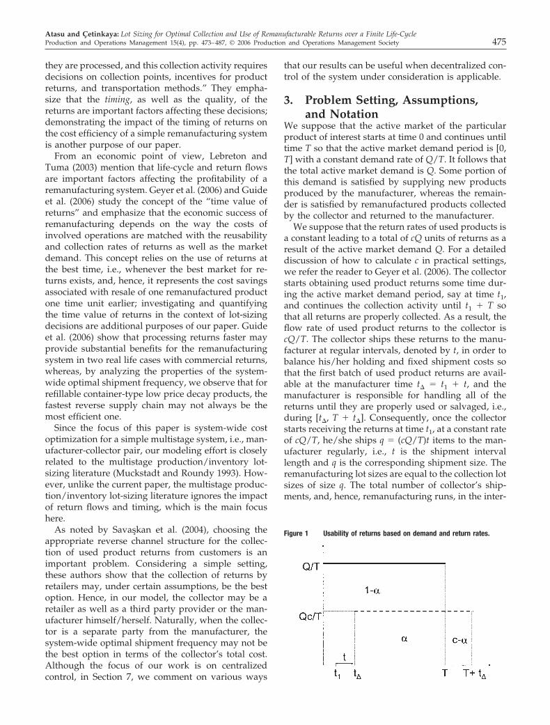
Figure 1 Usability of returns based on demand and return rates.

Atasu and Cetinkaya: Lot Sizing for Optimal Collection and Use of Remanufacturable Returns over a Finite Life-CycleProduction and Operations Management 15(4), pp. 473–487, © 2006 Production and Operations Management Society 475

val (t�, T � t�) is an integer, denoted by n. That is, n� T/t � cQ/q.

Figure 1 illustrates how the active market demandand used product returns flows are modelled over thelife-cycle of the product. Since all remanufacturedproducts are perfectly substitutable for satisfying thedemand for new products, and remanufacturing costsless, the manufacturer would like to cover demandusing as many remanufactured products as possible inorder to reduce the total cost. Observe that if t� equalszero, all of the returns can be used in the active mar-ket. Otherwise, only a certain percentage of the re-turns can be used in the active market. This percentageis denoted by �, and, by definition, �.Q � cQ(T� t�)/T so that

� �c�T � t� �

T . (1)

Obviously, a critical time interval in the process ofmarketing the remanufactured products is the collec-tor’s shipment interval length t, i.e., the time spentduring the collection phase. This is because t has animmediate impact on t� � t1 � t, the first time theremanufactured products enter the market, as well ason the future times that the remanufactured productsare ready for satisfying the market demand. By opti-mizing t, we enable the optimal use of remanufacturedproducts during the active market demand periodwhile at the same time improving system-wide prof-itability. Furthermore, we argue that our results onhow to compute the optimal t value provide an intu-itive way of understanding the concept of the timevalue of returns in this setting.

Our Main Model considers the case where the man-ufacturer replenishes his/her new product inventoryby producing at a finite rate P, incurring a fixed setupcost SN and a per-unit manufacturing cost p1. Since theproblem of interest is motivated by refillable containermanufacturing, producing new products requiresmore effort and time than remanufacturing used prod-uct returns, so a finite production rate of P is associ-ated with a new product production lot. Our MainModel concentrates on the case where a single pro-duction lot of new items is produced by the manufac-turer early in the active market demand period. Notethat the single production lot assumption is represen-tative of practice in those cases where the life cycle Tis short or set-up cost SN is relatively high, and thecorresponding lot-size is denoted by Q1. This quantityis known as the seed inventory level in practice (Ak-calı and Morse 2004). Our Main Model is built on theassumption that remanufacturing activity can be per-formed instantaneously by incurring a fixed remanu-facturing set-up cost SM and a per-unit remanufactur-ing cost p2 for each returned unit. However, a fixed

remanufacturing lead time can be modelled in astraightforward fashion. Also, we consider a per-unitper-unit-time holding cost hM for each item in themanufacturer’s inventory. We do not differentiate be-tween the holding costs of new and remanufacturedproducts since holding costs represent opportunitycosts based on market value, and we consider a prac-tical application where new and remanufacturedproducts are perfectly substitutable and have the samemarket value. In addition, we consider a per-unit per-unit-time holding cost hC for each return waiting to beshipped to the manufacturer in the collector’s usedproduct return inventory and a fixed delivery cost SC

associated with each shipment of used product re-turns from the collector to the manufacturer.

For our Main Model, the resulting cost optimizationproblem is relatively complicated. As a result, al-though we are able to provide an easy-to-implementnumerical optimization approach and insightful nu-merical results, this model leads to fewer analyticalinsights about one of the basic issues we investigate:the time value of returns. Fortunately, considering twospecial-yet, practically meaningful-cases, we providefurther analytical and insightful results. In SpecialCase 1, the manufacturer does not carry inventory andobtains new products from an external source withample supply (or producing at an infinite rate) incur-ring a per-unit (linear) cost only. In other words, SM

� 0, hM � 0, and P � �. In Special Case 2, themanufacturer replenishes his/her new product inven-tory once at the beginning of the active market de-mand period by obtaining the total number of itemshe/she needs from an external source with amplesupply incurring a fixed plus linear cost. In otherwords, P � �.

Special Case 1 leads to a closed form solution for theoptimal value of t that enables the timely use of re-turns in the active market in an economical way byminimizing the system-wide cost. This closed formsolution allows us to provide an intuitive illustrationof the time value of returns in the correspondingsetting. Naturally, in Special Case 2 and the MainModel, the system wide cost functions have morecomplicated forms which do not lead to closed formoptimal solutions. Nonetheless, by utilizing the ana-lytical properties of these cost functions, we can de-velop simple methods for computing the optimal so-lutions, and our results can be used to illustrate thetime value of returns for the collector-manufacturerpair.

In summary, the fundamental assumptions of ourmodeling effort are as follows:A1: Deterministic environment.A2: Perfect substitution of new and remanufactured

products.A3: Finite life-cycle.


A4: Single (initial) lot for new products resulting in afixed amount of seed inventory.

A5: Negligible delivery lead times from the collectorto the manufacturer.

A6: Instantaneous remanufacturing.A7: Identical holding costs for new and remanufac-

tured product inventories.We consider a deterministic environment for analyti-cal ease, and we place emphasis on providing practicalinsights via presenting analytical as well as numericalresults. We note, however, that various challengingextensions with stochastic demand/return flows andproduction/remanufacturing lead times remain forfuture research for which the current paper providesonly a rough, approximate analysis by studying theimpact of timing, as well as lot-sizing and flow coor-dination. We also reiterate that, as discussed in detailin Section 1, our assumptions regarding perfect sub-stitution and finite life cycle are reasonable and rep-resentative of practice for the motivating examples ofour analytical work, i.e., for products of refillable con-tainer remanufacturing such as printer cartridges andsingle use cameras.

Since Special Cases 1 and 2 provide a foundation fordetailed results and insightful interpretations for ourMain Model, we proceed with a detailed discussion ofthese two cases. Before concluding this section, wenote that Table 1 provides a summary of the notationintroduced so far and introduces some additional no-tation that will be used in the subsequent develop-ment.

4. Special Cases4.1. Special Case 1 (SM � 0, hM � 0, and P � �)In this case, the manufacturer’s fixed replenishmentand holding costs are ignored. Then, recalling thatmanufacturing/remanufacturing activity takes placeover [0, T] whereas collection activity takes place over[t1, T � t�], the cost of manufacturing over [0, T] isgiven by p1(1 � �)Q, and the cost of remanufacturingis given by p2�Q, so the total manufacturing/remanu-facturing cost is

� p1 �1 � �� p2��Q, (2)

where � is given by Expression (1). Note that theprocessing costs associated with returns arriving at themanufacturer after the active market demand periodare not included in this cost model, since, without lossof generality, we assume that these items can be sal-vaged at no cost. If these items can be sold for morethan p2, say there exists a salvage income of p3 peritem, then the total manufacturing/remanufacturingcost is (p1(1 � �) � p2� � p3(c � �))Q, which is merelyequivalent to Expression (2). Also, it can be easily shownthat the collection cost over [t1, T � t�] is given by

SC n �cQThC

2n ,

Using Expression (1) and recalling that t� � t1 � t andn � T/t, we express the sum of the manufacturing/remanufacturing and collection costs as a function of nonly. As a result, the total cost for Special Case 1 isgiven by

TC � A �BTn �

CnT , where (3)

A � Qp1 � Q� p1 � p2 �c � Q� p1 � p2 �c�t1 �/T,

B � Q� p1 � p2 �c/T � cQhC / 2, and C � TSC .

Proposition 1. For Special Case 1, the optimal numberof shipments, denoted by n*, is given by

n* � � arg min{TC( n� ), TC( n� )}, n� � (1, cQ )arg min1, cQ {TC(n)}, o/w

(4)

where x denotes the largest integer less than or equal to x, x denotes the smallest integer greater than or equal to x,and n� � TB/C. The optimal values for t, t�, and q aregiven by t* � T/n*, t*� � t1 � T/n*, and q* � cQ/n*,respectively.

Proof. All proofs are presented in the Appen-dix. �

Based on this result, we argue that n* and, hence, t*,provide an indication of the time value of returns. Thisis simply because a large n* value implies a small t*

Table 1 Notation

T The length of the active market demand interval.t1 Consumer lead time, i.e., the time when the collector starts receiving the

returns.t� The time when the remanufactured products are ready for the active

market for the first time, i.e., at t�, the used products returns havebeen shipped to the manufacturer and remanufactured.

Q Total demand in the active market.c Return rate, i.e., a constant leading to a collection rate of cQ/T.� Percentage of returns (over total demand) used during the active market.Q1 Represents the corresponding inventory level illustrated in Figures 2, 5,

and 4.Q2 Represents the corresponding inventory level illustrated in Figure 5.Q3 Represents the corresponding inventory level illustrated in Figure 5.t Collector’s shipment interval length.q Collector’s shipment size and remanufacturing lot size.p1 Manufacturer’s unit cost for a new product.p2 Manufacturer’s unit cost for a remanufactured product.p p1 � p2.SM Manufacturer’s set-up cost for remanufacturing.hM Manufacturer’s per-unit per-unit time holding cost.SC Collector’s set-up (fixed shipment) cost.hC Collector’s per-unit per-unit time holding cost.TC Total (system-wide) cost of the manufacturer and the collector.


value which, in turn, implies a faster reverse supplychain with frequent shipments from the collector tothe manufacturer as an indication of a high time valueof returns.

Expression (4) implies that the exact t* value needsto be computed numerically. However, if n� � (1, cQ ), then a closed-form approximation for the ship-ment frequency is given by

t� �Tn�

� �CB � � TSC

cQ�p1 � p2

T �hC

2 � . (5)

Observe that Expression (5) looks very similar to theoptimal cycle length of the classical economic orderquantity (EOQ) model for which the order frequencyis given as t* � 2S/�h, where S is the set-up cost, his the holding cost, and � is the demand rate. There aretwo main differences. First, the demand rate in theoptimal cycle length formula of the classical EOQmodel is replaced by cQ/T, the collection rate, inExpression (5). Second, we have an additional term, i.e.,

v �p1 � p2

T , (6)

in the denominator in the square root. We argue that vrepresents the average cost of holding one unit of a usedproduct return in collector’s inventory for an additionaltime unit rather than shipping it for the active market.Hence, v can be used as an estimate for the time value ofa used product return. Also, observe that, v is decreasing inT whereas t� is increasing in T, both of which imply thatthe longer the life-cycle of the product, the lower thetime value of returns. Furthermore, the difference be-tween p1 and p2 affects v. That is, the higher the differ-ence in the unit cost of a new and a remanufacturedproduct, the higher is the time value. Finally, we notethat Expression (5) does not depend on t1, so the ship-ment interval length is independent of the time the usedproducts stay with the original customers. However, inthe next section we show that this is no longer true if weconsider the manufacturer’s inventory-related costs ex-plicitly.

4.2. Special Case 2 (P � �)In this case, the manufacturer receives (from an exter-nal source with ample supply or by producing at aninfinite rate) an initial replenishment quantity, i.e.,seed inventory, of new products, denoted by Q1, foronce early in the active market demand period incur-ring a fixed cost, denoted by SN. The used productreturns are remanufactured at a fixed cost of SM, andthey incur a per-unit per-unit time holding cost de-noted by hM. We also note that, without loss of gen-erality, we can assume that SN � 0, as the initial setupcost is a sunk cost under the fixed demand (i.e., no lost

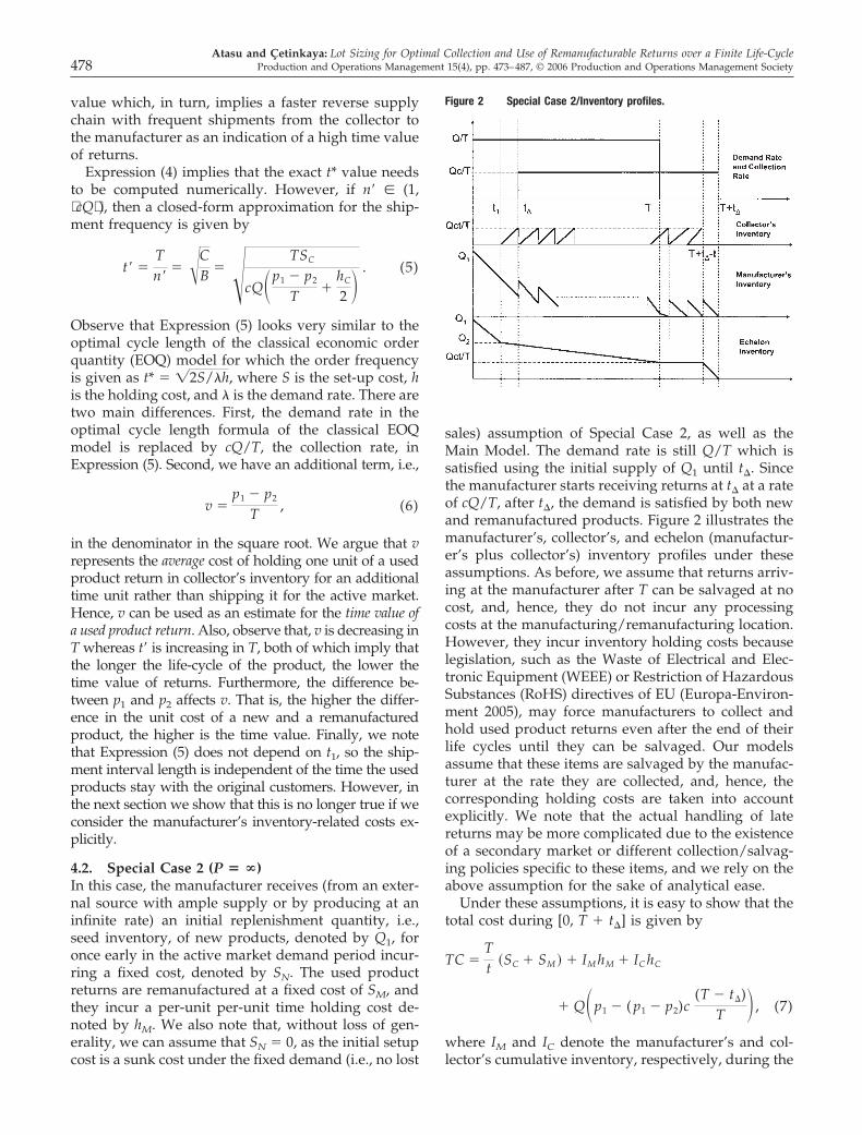
sales) assumption of Special Case 2, as well as theMain Model. The demand rate is still Q/T which issatisfied using the initial supply of Q1 until t�. Sincethe manufacturer starts receiving returns at t� at a rateof cQ/T, after t�, the demand is satisfied by both newand remanufactured products. Figure 2 illustrates themanufacturer’s, collector’s, and echelon (manufactur-er’s plus collector’s) inventory profiles under theseassumptions. As before, we assume that returns arriv-ing at the manufacturer after T can be salvaged at nocost, and, hence, they do not incur any processingcosts at the manufacturing/remanufacturing location.However, they incur inventory holding costs becauselegislation, such as the Waste of Electrical and Elec-tronic Equipment (WEEE) or Restriction of HazardousSubstances (RoHS) directives of EU (Europa-Environ-ment 2005), may force manufacturers to collect andhold used product returns even after the end of theirlife cycles until they can be salvaged. Our modelsassume that these items are salvaged by the manufac-turer at the rate they are collected, and, hence, thecorresponding holding costs are taken into accountexplicitly. We note that the actual handling of latereturns may be more complicated due to the existenceof a secondary market or different collection/salvag-ing policies specific to these items, and we rely on theabove assumption for the sake of analytical ease.

Under these assumptions, it is easy to show that thetotal cost during [0, T � t�] is given by

TC �Tt �SC � SM � � IM hM � IC hC

� Q�p1 � ( p1 � p2)c(T � t�)

T � , (7)

where IM and IC denote the manufacturer’s and col-lector’s cumulative inventory, respectively, during the

Figure 2 Special Case 2/Inventory profiles.


planning horizon. Letting IE denote the cumulativeechelon inventory and using Figure 2, IC and IM can becomputed as follows:

IC �cQt

2 , (8)

IM � IE � IC , where (9)

IE � �Q1 � Q2

2 � t1 � �Q2 � Q3

2 � �T � t1 � �cQtt1

T

�cQt2

2T ,

Q1 � Q �cQ�T � t� �

T ,

Q2 � Q1 �Qt1

T , and

Q3 �cQt

T .

Substituting the above set of equations in Expression(7), we have

TC � A � Bt � Ct2 �Dt , (10)

where A is a constant, and, hence, can be ignored forour purposes,

B �cQ2 �hM � hC �

2( p1 � p2 � hM t1)T � ,

C �chM Q

2T , and D � �SM � SC�T. (11)

As in the previous section, Expression (10) can beexpressed in terms of n so that we have

TC � A �BTn �

CT2

n2 �DnT . (12)

Proposition 2. For Special Case 2, the optimal numberof shipments, denoted by n*, is given by

n* � � arg min{TC( n� ), TC( n� )}, n� � (1, cQ ),arg min1, cQ{TC(n)}, o/w,

where

n� � �3 R � �K � �3 R � �K, K � L3 � R2,

L � �BT2

3D , and R �CT3

D .

It follows that t* � T/n*, t*� � t1 � T/n*, and q* � cQ/n*.Also, the optimal initial replenishment quantity Q1 , i.e., theoptimal seed inventory, is given by

Q*1 � Q �

cQ�T � t1 �Tn*�

T .

Here, unlike Special Case 1, we are not able toobtain a closed form approximation for t* which im-plicitly suggests an estimate for the time value of a usedproduct return. Although the exact t* value needs to becomputed numerically, if n� � (1, cQ ), then t� � T/n�still provides a numerical approximation for t*. Basedon this observation, we obtain analytical results inves-tigating the relationship between t*, t�, and the criticalmodel parameters as summarized in Corollary 1.

Corollary 1. For Special Case 2, t� (as an approxima-tion for t*) is increasing in SC, SM, and T whereas it isdecreasing in t1 , hM, hC, c, and p � p1 � p2.

One key observation for Special Case 2 is that, sincet1 is included in term B of the cost function given byExpression (12), t* depends on t1. That is, unlike Spe-cial Case 1, the amount of time used product returnsstay with the original customers (consumer lead time)has an effect on the timing, and, hence, the time value,of the returns. According to Corollary 1, t� (as anapproximation for t*) is decreasing in t1, and, hence,the later we start collecting used product returns fromthe original customers, the faster the collection chan-nel should be. Another important observation is that,similar to Special Case 1, the shipment interval lengthincreases, and, thus, the time value of returns, de-creases with increasing life cycle length T. This is dueto the fact that the opportunity for reusing returns isnot lost as quickly under longer life cycles, and, there-fore, the system can afford to wait longer for largershipments of returns to accumulate. On the otherhand, the shipment frequency increases with increas-ing c, and, hence, with increasing collection rate cQ/T.Since a higher c value implies that the availability ofreturns is higher, the potential savings from a fastercollection channel is higher. This, in turn, results in ahigher shipment frequency. The effects of inventoryholding and set-up costs on the shipment frequencyare similar to the results from the classical EOQ for-mula, i.e., shipment frequency increases as holdingcosts hM and hC increase and decreases as fixed costsSM and SC increase.

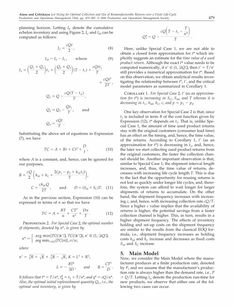
5. Main ModelNow, we consider the Main Model where the manu-facturer produces at a finite production rate, denotedby P, and we assume that the manufacturer’s produc-tion rate is always higher than the demand rate, i.e., P Q/T. Letting t� denote the production run-time fornew products, we observe that either one of the fol-lowing two cases can occur.


• Case a:

t� � �QT � cQT � cQt1 � PTt1

PT � 2cQ � .

This case occurs when the production rate ofthe manufacturer is sufficiently high so that theproduction of the initial production quantity ofnew products ends before t� (see Figure 3a foran illustration of the echelon inventory profilein this case.)

• Case b:

t� � �QT � cQT � cQt1 � PTt1

PT � 2cQ � .

This case occurs when the production of theinitial lot of new products ends after t� (seeFigure 3b for an illustration of the echelon in-ventory profile in this case).As in Special Case 2, the total cost during [0, T� t�] is given by Expression (7). However, weneed to compute the relevant expressions of IM

and IC. Observe that in both cases, as in SpecialCase 2, IC and IM are given by Expressions (8)and (9), respectively. In Appendix, we developthe total cost expressions for Cases a and b, andwe show that these expressions are equivalentfor optimization purposes. That is, the minimiz-ers of both functions are the same as the mini-mizer of

TC� � Bt � Ct2 �Dt , (13)

where B, C, and D are given by Expression (24) inAppendix. Again, as for Special Cases 1 and 2, thiscost function can be written in terms of n so that wehave

TC� �BTn �

CT2

n2 �DnT . (14)

Proposition 3.

• For the Main Model, if B � 0 and C � 0, then theoptimal number of shipments, denoted by n*, isgiven by either � 1 or cQ , depending on whichone leads to a lower TC� value.

• If B � 0 and C � 0, then the optimal number ofshipments, denoted by n*, is given byn*

� � arg min{TC( n� ), TC( n� )}, n� � (1, cQ )arg min1, cQ �TC(n)}, o/w

(15)

where n� is the unique positive real root of thefirst derivative of TC�.

• In other cases, i.e., (B 0, C � 0) and (B � 0, C 0), the optimal solution can be computed easilyby (i) partitioning the domain of TC� into tworegions as illustrated in Figure 4, (ii) computingthe appropriate positive real root of the first de-rivative of TC�, and (iii) replacing the value of thisroot with n� in the above expression of n*.

In this case, unlike in Special Cases 1 and 2, we arenot able to obtain analytical results that implicitlysuggest an estimate for the time value of a used productreturn. This is due to the non-convex nature of theunderlying cost function. However, using Proposition3, it is straightforward to obtain numerical results.Hence, we rely on such results for insights.

Before proceeding with a detailed discussion of ournumerical results, it is worth examining under whatconditions the underlying cost function is convex.

Figure 3 Main Model/Echelon inventory profiles.


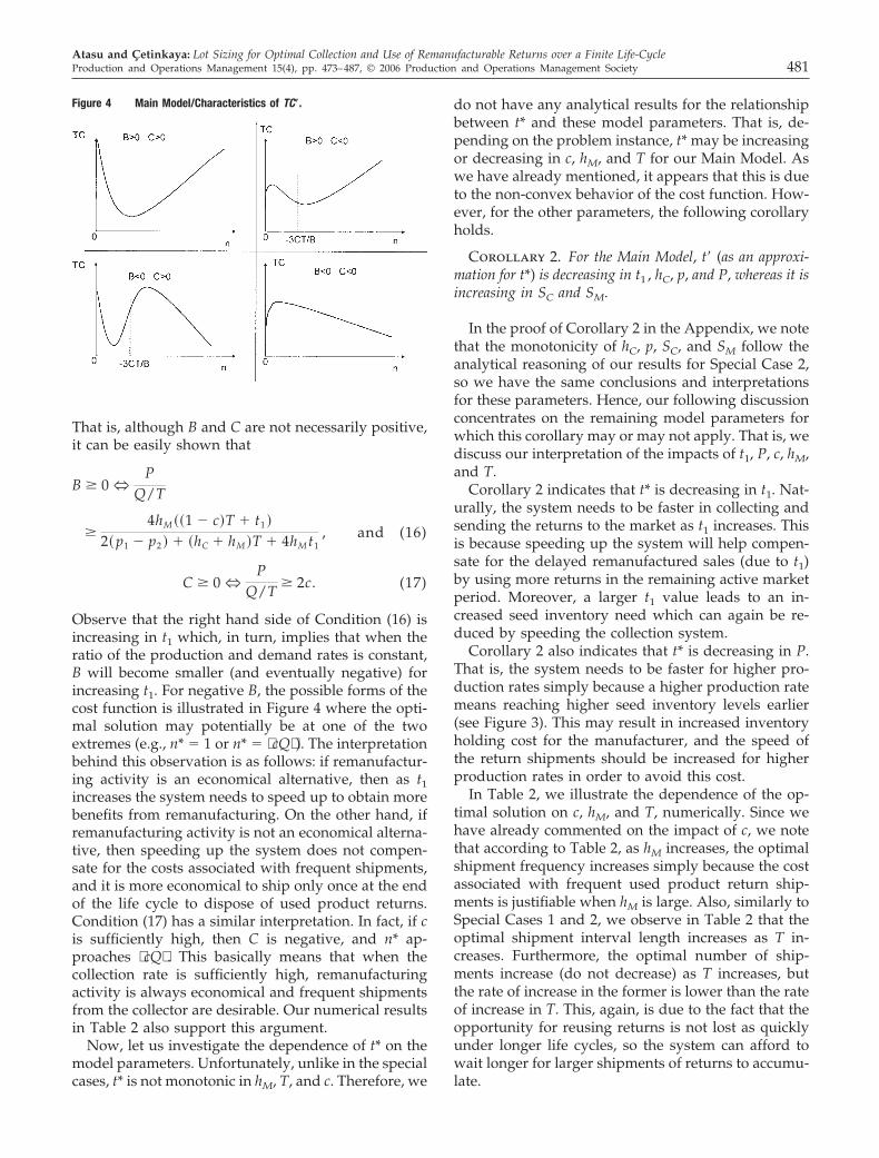
That is, although B and C are not necessarily positive,it can be easily shown that

B � 0 NP

Q/T

�4hM ��1 � c�T � t1 �

2� p1 � p2 � � �hC � hM �T � 4hM t1, and (16)

C � 0 NP

Q/T � 2c. (17)

Observe that the right hand side of Condition (16) isincreasing in t1 which, in turn, implies that when theratio of the production and demand rates is constant,B will become smaller (and eventually negative) forincreasing t1. For negative B, the possible forms of thecost function is illustrated in Figure 4 where the opti-mal solution may potentially be at one of the twoextremes (e.g., n* � 1 or n* � cQ ). The interpretationbehind this observation is as follows: if remanufactur-ing activity is an economical alternative, then as t1increases the system needs to speed up to obtain morebenefits from remanufacturing. On the other hand, ifremanufacturing activity is not an economical alterna-tive, then speeding up the system does not compen-sate for the costs associated with frequent shipments,and it is more economical to ship only once at the endof the life cycle to dispose of used product returns.Condition (17) has a similar interpretation. In fact, if cis sufficiently high, then C is negative, and n* ap-proaches cQ . This basically means that when thecollection rate is sufficiently high, remanufacturingactivity is always economical and frequent shipmentsfrom the collector are desirable. Our numerical resultsin Table 2 also support this argument.

Now, let us investigate the dependence of t* on themodel parameters. Unfortunately, unlike in the specialcases, t* is not monotonic in hM, T, and c. Therefore, we

do not have any analytical results for the relationshipbetween t* and these model parameters. That is, de-pending on the problem instance, t* may be increasingor decreasing in c, hM, and T for our Main Model. Aswe have already mentioned, it appears that this is dueto the non-convex behavior of the cost function. How-ever, for the other parameters, the following corollaryholds.

Corollary 2. For the Main Model, t� (as an approxi-mation for t*) is decreasing in t1 , hC, p, and P, whereas it isincreasing in SC and SM.

In the proof of Corollary 2 in the Appendix, we notethat the monotonicity of hC, p, SC, and SM follow theanalytical reasoning of our results for Special Case 2,so we have the same conclusions and interpretationsfor these parameters. Hence, our following discussionconcentrates on the remaining model parameters forwhich this corollary may or may not apply. That is, wediscuss our interpretation of the impacts of t1, P, c, hM,and T.

Corollary 2 indicates that t* is decreasing in t1. Nat-urally, the system needs to be faster in collecting andsending the returns to the market as t1 increases. Thisis because speeding up the system will help compen-sate for the delayed remanufactured sales (due to t1)by using more returns in the remaining active marketperiod. Moreover, a larger t1 value leads to an in-creased seed inventory need which can again be re-duced by speeding the collection system.

Corollary 2 also indicates that t* is decreasing in P.That is, the system needs to be faster for higher pro-duction rates simply because a higher production ratemeans reaching higher seed inventory levels earlier(see Figure 3). This may result in increased inventoryholding cost for the manufacturer, and the speed ofthe return shipments should be increased for higherproduction rates in order to avoid this cost.

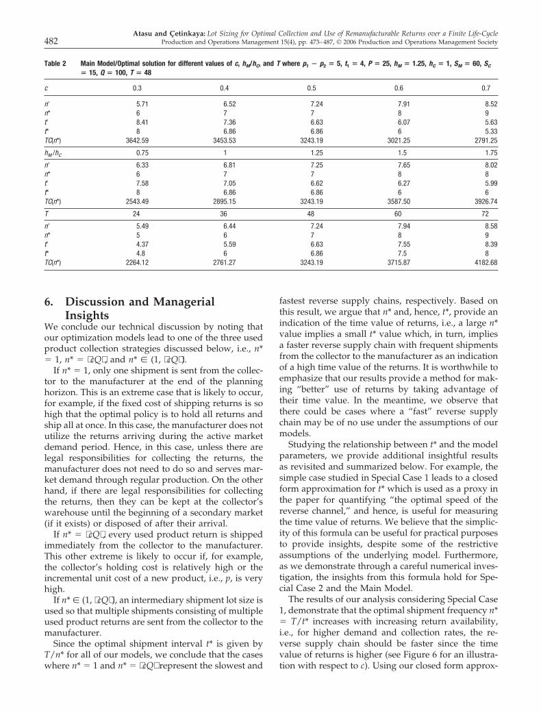
In Table 2, we illustrate the dependence of the op-timal solution on c, hM, and T, numerically. Since wehave already commented on the impact of c, we notethat according to Table 2, as hM increases, the optimalshipment frequency increases simply because the costassociated with frequent used product return ship-ments is justifiable when hM is large. Also, similarly toSpecial Cases 1 and 2, we observe in Table 2 that theoptimal shipment interval length increases as T in-creases. Furthermore, the optimal number of ship-ments increase (do not decrease) as T increases, butthe rate of increase in the former is lower than the rateof increase in T. This, again, is due to the fact that theopportunity for reusing returns is not lost as quicklyunder longer life cycles, so the system can afford towait longer for larger shipments of returns to accumu-late.

Figure 4 Main Model/Characteristics of TC�.


6. Discussion and ManagerialInsights

We conclude our technical discussion by noting thatour optimization models lead to one of the three usedproduct collection strategies discussed below, i.e., n*� 1, n* � cQ , and n* � (1, cQ ).

If n* � 1, only one shipment is sent from the collec-tor to the manufacturer at the end of the planninghorizon. This is an extreme case that is likely to occur,for example, if the fixed cost of shipping returns is sohigh that the optimal policy is to hold all returns andship all at once. In this case, the manufacturer does notutilize the returns arriving during the active marketdemand period. Hence, in this case, unless there arelegal responsibilities for collecting the returns, themanufacturer does not need to do so and serves mar-ket demand through regular production. On the otherhand, if there are legal responsibilities for collectingthe returns, then they can be kept at the collector’swarehouse until the beginning of a secondary market(if it exists) or disposed of after their arrival.

If n* � cQ , every used product return is shippedimmediately from the collector to the manufacturer.This other extreme is likely to occur if, for example,the collector’s holding cost is relatively high or theincremental unit cost of a new product, i.e., p, is veryhigh.

If n* � (1, cQ ), an intermediary shipment lot size isused so that multiple shipments consisting of multipleused product returns are sent from the collector to themanufacturer.

Since the optimal shipment interval t* is given byT/n* for all of our models, we conclude that the caseswhere n* � 1 and n* � cQ represent the slowest and

fastest reverse supply chains, respectively. Based onthis result, we argue that n* and, hence, t*, provide anindication of the time value of returns, i.e., a large n*value implies a small t* value which, in turn, impliesa faster reverse supply chain with frequent shipmentsfrom the collector to the manufacturer as an indicationof a high time value of the returns. It is worthwhile toemphasize that our results provide a method for mak-ing “better” use of returns by taking advantage oftheir time value. In the meantime, we observe thatthere could be cases where a “fast” reverse supplychain may be of no use under the assumptions of ourmodels.

Studying the relationship between t* and the modelparameters, we provide additional insightful resultsas revisited and summarized below. For example, thesimple case studied in Special Case 1 leads to a closedform approximation for t* which is used as a proxy inthe paper for quantifying “the optimal speed of thereverse channel,” and hence, is useful for measuringthe time value of returns. We believe that the simplic-ity of this formula can be useful for practical purposesto provide insights, despite some of the restrictiveassumptions of the underlying model. Furthermore,as we demonstrate through a careful numerical inves-tigation, the insights from this formula hold for Spe-cial Case 2 and the Main Model.

The results of our analysis considering Special Case1, demonstrate that the optimal shipment frequency n*� T/t* increases with increasing return availability,i.e., for higher demand and collection rates, the re-verse supply chain should be faster since the timevalue of returns is higher (see Figure 6 for an illustra-tion with respect to c). Using our closed form approx-

Table 2 Main Model/Optimal solution for different values of c, hM/hC, and T where p1 � p2 � 5, t1 � 4, P � 25, hM � 1.25, hC � 1, SM � 60, SC

� 15, Q � 100, T � 48

c 0.3 0.4 0.5 0.6 0.7

n� 5.71 6.52 7.24 7.91 8.52n* 6 7 7 8 9t� 8.41 7.36 6.63 6.07 5.63t* 8 6.86 6.86 6 5.33TC(n*) 3642.59 3453.53 3243.19 3021.25 2791.25

hM /hC 0.75 1 1.25 1.5 1.75

n� 6.33 6.81 7.25 7.65 8.02n* 6 7 7 8 8t� 7.58 7.05 6.62 6.27 5.99t* 8 6.86 6.86 6 6TC(n*) 2543.49 2895.15 3243.19 3587.50 3926.74

T 24 36 48 60 72

n� 5.49 6.44 7.24 7.94 8.58n* 5 6 7 8 9t� 4.37 5.59 6.63 7.55 8.39t* 4.8 6 6.86 7.5 8TC(n*) 2264.12 2761.27 3243.19 3715.87 4182.68


imation for t*, we observe that the time value of re-turns increases with return availability cQ andincremental cost of remanufacturing p, whereas it de-creases with the life cycle length T. The formula alsoindicates that the effects of inventory related costs ont* is similar to those established in the production/inventory literature, i.e., the shipment frequency in-creases in holding costs and decreases in set-up costs.

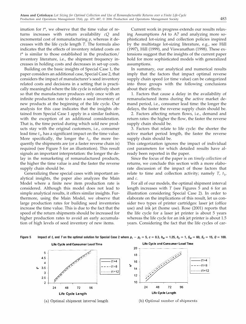
Building on the basic insights of Special Case 1, thepaper considers an additional case, Special Case 2, thatconsiders the impact of manufacturer’s seed inventoryrelated costs and decisions in a setting that is practi-cally meaningful where the life cycle is relatively shortso that the manufacturer produces only once with aninfinite production rate to obtain a seed inventory ofnew products at the beginning of the life cycle. Ouranalysis for this case indicates that the insights ob-tained from Special Case 1 apply in a similar fashion,with the exception of an additional consideration.That is, the time period during which sold new prod-ucts stay with the original customers, i.e., consumerlead time t1, has a significant impact on the time value.More specifically, the longer the t1, the more fre-quently the shipments are (or a faster reverse chain is)required (see Figure 5 for an illustration). This resultsignals an important interpretation: the longer the de-lay in the remarketing of remanufactured products,the higher the time value is and the faster the reversesupply chain should be.

Generalizing these special cases with important an-alytical insights, the paper also analyzes the MainModel where a finite new item production rate isconsidered. Although this model does not lead tosimple analytical results, it offers similar insights. Fur-thermore, using the Main Model, we observe thatlarge production rates for building seed inventoriesincrease the time value. This is due to the fact that thespeed of the return shipments should be increased forhigher production rates to avoid an early accumula-tion of high levels of seed inventory of new items.

Current work in progress extends our results relax-ing Assumptions A4 to A7 and analyzing more so-phisticated lot-sizing and collection policies inspiredby the multistage lot-sizing literature, e.g., see Hill(1997), Hill (1999), and Viswanathan (1998). These ex-tensions suggest that the insights of the current paperhold for more sophisticated models with generalizedassumptions.

In summary, our analytical and numerical resultsimply that the factors that impact optimal reversesupply chain speed (or time value) can be categorizedinto three groups with the following conclusionsabout their effects:

1. Factors that cause a delay in the availability ofremanufactured items during the active market de-mand period, i.e., consumer lead time: the longer thedelays, the faster the reverse supply chain should be.

2. Factors affecting return flows, i.e., demand andreturn rates: the higher the flow, the faster the reversesupply chain should be.

3. Factors that relate to life cycle: the shorter theactive market period length, the faster the reversesupply chain should be.This categorization ignores the impact of individualcost parameters for which detailed results have al-ready been reported in the paper.

Since the focus of the paper is on timely collection ofreturns, we conclude this section with a more elabo-rate discussion of the impact of those factors thatrelate to time and collection activity; namely T, t1,and c.

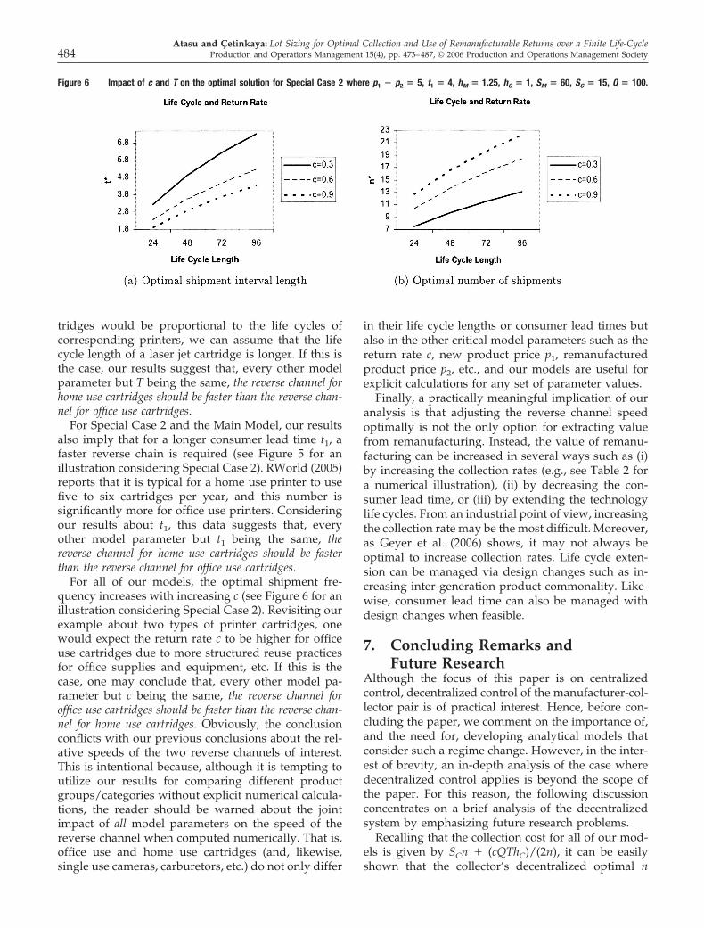
For all of our models, the optimal shipment intervallength increases with T (see Figures 5 and 6 for anillustration considering Special Case 2). In order toelaborate on the implications of this result, let us con-sider two types of printer cartridges: laser jet (officeuse) and ink jet (home use). Rose (2001) reports thatthe life cycle for a laser jet printer is about 5 yearswhereas the life cycle for an ink jet printer is about 1.5years. Considering the fact that the life cycles of car-

Figure 5 Impact of t1 and T on the optimal solution for Special Case 2 where p1 � p2 � 5, c � 0.3, hM � 1.25, hC � 1, SM � 60, SC � 15, Q � 100.


tridges would be proportional to the life cycles ofcorresponding printers, we can assume that the lifecycle length of a laser jet cartridge is longer. If this isthe case, our results suggest that, every other modelparameter but T being the same, the reverse channel forhome use cartridges should be faster than the reverse chan-nel for office use cartridges.

For Special Case 2 and the Main Model, our resultsalso imply that for a longer consumer lead time t1, afaster reverse chain is required (see Figure 5 for anillustration considering Special Case 2). RWorld (2005)reports that it is typical for a home use printer to usefive to six cartridges per year, and this number issignificantly more for office use printers. Consideringour results about t1, this data suggests that, everyother model parameter but t1 being the same, thereverse channel for home use cartridges should be fasterthan the reverse channel for office use cartridges.

For all of our models, the optimal shipment fre-quency increases with increasing c (see Figure 6 for anillustration considering Special Case 2). Revisiting ourexample about two types of printer cartridges, onewould expect the return rate c to be higher for officeuse cartridges due to more structured reuse practicesfor office supplies and equipment, etc. If this is thecase, one may conclude that, every other model pa-rameter but c being the same, the reverse channel foroffice use cartridges should be faster than the reverse chan-nel for home use cartridges. Obviously, the conclusionconflicts with our previous conclusions about the rel-ative speeds of the two reverse channels of interest.This is intentional because, although it is tempting toutilize our results for comparing different productgroups/categories without explicit numerical calcula-tions, the reader should be warned about the jointimpact of all model parameters on the speed of thereverse channel when computed numerically. That is,office use and home use cartridges (and, likewise,single use cameras, carburetors, etc.) do not only differ

in their life cycle lengths or consumer lead times butalso in the other critical model parameters such as thereturn rate c, new product price p1, remanufacturedproduct price p2, etc., and our models are useful forexplicit calculations for any set of parameter values.

Finally, a practically meaningful implication of ouranalysis is that adjusting the reverse channel speedoptimally is not the only option for extracting valuefrom remanufacturing. Instead, the value of remanu-facturing can be increased in several ways such as (i)by increasing the collection rates (e.g., see Table 2 fora numerical illustration), (ii) by decreasing the con-sumer lead time, or (iii) by extending the technologylife cycles. From an industrial point of view, increasingthe collection rate may be the most difficult. Moreover,as Geyer et al. (2006) shows, it may not always beoptimal to increase collection rates. Life cycle exten-sion can be managed via design changes such as in-creasing inter-generation product commonality. Like-wise, consumer lead time can also be managed withdesign changes when feasible.

7. Concluding Remarks andFuture Research

Although the focus of this paper is on centralizedcontrol, decentralized control of the manufacturer-col-lector pair is of practical interest. Hence, before con-cluding the paper, we comment on the importance of,and the need for, developing analytical models thatconsider such a regime change. However, in the inter-est of brevity, an in-depth analysis of the case wheredecentralized control applies is beyond the scope ofthe paper. For this reason, the following discussionconcentrates on a brief analysis of the decentralizedsystem by emphasizing future research problems.

Recalling that the collection cost for all of our mod-els is given by SCn � (cQThC)/(2n), it can be easilyshown that the collector’s decentralized optimal n

Figure 6 Impact of c and T on the optimal solution for Special Case 2 where p1 � p2 � 5, t1 � 4, hM � 1.25, hC � 1, SM � 60, SC � 15, Q � 100.


value that minimizes his/her own cost only is givenby ncol � arg min{TCcol( n�col ), TC( n�col )} where n�col

� cQhCT/(2SC). For all of our models, since ncol maybe different than n*, the collector has to be convincedto use the system optimal n value, i.e., n*, instead ofusing ncol. Recall also that for all of our models, thejoint total cost is given by TC(n) and that it is the sumof the collector’s cost, denoted by TCcol(n), and themanufacturer’s cost, denoted by TCman(n). It can beeasily shown that TCman(ncol) � TCman(n*) � TCcol(n*)� TCcol(ncol), which, in turn, implies that, at the systemoptimal, the collector’s loss can be compensated forfrom the decrease in the total system cost, and, aftercompensation, the manufacturer’s cost decrease isgreater than or equal to zero. It is important to notethat since the underlying cost functions of our modelsare not necessarily convex and continuous, quantity-based coordination mechanisms, such as all-units andincremental quantity reward schemes, may not be use-ful for coordination in general (see Toptal andCetinkaya 2006) for an illustration of coordination is-sues under rather general cost functions). On the otherhand, simple coordination mechanisms that build onthe idea of offering the collector a side benefit on atake-it-or-leave-it basis can be developed for our prob-lems in a straightforward fashion, and, hence, thedetails of this development are omitted here. How-ever, a numerical investigation of other practicalmechanisms that can be effectively implemented astrading agreements and linked to the decisions of thetwo parties remains an area for future investigation.

Several other important issues pertaining to the de-centralized control of the manufacturer-collector pairalso remain open for future research. These includeprivate information considerations and individual in-centives. Naturally, centralized models developed inthis paper provide a foundation for this line of futureresearch since analytical models under centralizedcontrol with full information provide benchmarks formeasuring the effectiveness of contractual decentral-ized control. In fact, there may be better centralizedoperational policies for the system under consider-ation in this paper where, for example, the manufac-turer and the collector implement more sophisticatedproduction and shipment policies with varying seedinventories and shipment intervals. An analytical in-vestigation of such general policies is a challengingproblem worthy of careful academic attention and itwill provide a foundation for future research on de-centralized control.

Finally, we note that the case where remanufactureditems are not perfectly substitutable for the new prod-ucts but can be marketed during the active marketdemand period at a lower price—which is the case forsome products in the electronics industry—also re-mains an interesting problem for future research.

AcknowledgmentsThe authors thank V. Daniel R. Guide, Luk N. Van Wassen-hove, an anonymous AE, and two anonymous referees fortheir helpful comments on earlier versions of the paper. Thisresearch was supported in part by NSF Grants CAREER/DMII-0093654 and DMII-0522980.

AppendixProof of Proposition 1. Since Expression (3) is a convex

function of n, the non-integer optimal n value, denoted byn�, is given by n� � TB/C. Hence, the optimal number ofshipments, denoted by n*, is given by n* � arg min{TC( n� ),TC( n� )}. Furthermore, n* cannot exceed the total number ofused product returns which is given by cQ . �

Proof of Proposition 2. Recalling Expression (12), we notethat B is a positive constant, simply because, by assumption,p1 � p2. Also, C and D are both positive. In order to provethe convexity of the cost function in Expression (12), weexamine its second derivative which is given by 2BT/n3

� 6CT2/n4. Obviously, n 0 so that the convexity conditioncan be written as BTn � 3CT2 � 0 which is always true, sinceall of the terms on the left hand side are positive. In addition,it can be easily shown that limn3� TC � � since D ispositive. Also, limn40 TC � � since B and C are bothpositive. Consequently, the real minimizer of the cost func-tion, denoted by n�, is unique. This, in turn, implies that theoptimal integer n value, denoted by n*, can be expressed asn* � arg min{TC( n� ), TC( n� )}. Obviously, n� is calculatedby setting the derivative of the total cost, with respect to n,equal to zero, i.e., using the following expression:

n3 � ��BT2

D �n � ��2CT3

D � � 0.

Observe that the right hand side of the above equation is athird order polynomial of the form n3 � an � b. The roots ofthis polynomial are given by (Wolfram Research-Mathworld2004)

n1 � M � N, n2 � ��M � N�

2 �i�3�M � N�

2 , and

n3 � ��M � N�

2 �i�3�M � N�

2 ,

where

M � �3 R � �K, N � �3 R � �K, K � L3 � R2,

L �a3 , and R �

b2 .

If the polynomial discriminant K 0, only one of these rootsis real and the others are complex. If K � 0, all roots are realand at least two are equal. If K � 0, all roots are real andunequal. However, using the convexity analysis, we knowthat for n 0 there is only one positive real root which wedenote by n�. Also, the values that n takes can only beintegers between 1 and cQ . �

Proof of Corollary 1. Using Expressions (10)–(11), it can beeasily verified that


2TCtt1

�cQhM

T� 0,

2TCthM

�cQ�2t � T � 2t1 �

2T� 0,

2TCthC

�cQ2 � 0,

2TCtSC

� ��Tt2� � 0,

2TCtSM

� ��Tt2� � 0,

2TCtc

�cQ2 � 0,

2TCtp

�cQT

� 0 and

2TCtT

� ��(SC � SM)T2 � cQt2(p1 � p2 � hM(t � t1))t2T2 � � 0.

It follows that t* is decreasing in t1 because TC is super-modular in t and t1. Since t* is the minimizer of TC, it isdecreasing in t1. Also, t* is decreasing in hM because TC issupermodular in t and hM. Similarly, t* is decreasing in hC, c,and p whereas it is increasing in SC, SM, and T. �

Total Cost Function for the Main ModelCase a: Using Figure 5, we have

IE �Q1 t�

2 ��Q1 � Q2 ��t� � t� �

2 ��Q3 � Q2 ��T � t� �

2

�cQtt1

T�

cQt2

2T, where

t� �Q2 � �Qt� �/T

P, (18)

Q1 � �P �QT� t� , (19)

Q2 �Q�1 � c��T � t� � � cQt

T, and (20)

Q3 �cQt

T. (21)

As a result, using Expression (9), we have

IM �Q1 t�

2 ��Q1 � Q2 ��t� � t� �

2 ��Q3 � Q2 ��T � t� �

2

�cQtt1

T�

cQt2

2T�

cQ2 t (22)

Observe that the last term in the equation represents thepotential inventory reduction in the system because of usingreturns instead of new products in the active market. Sub-stituting Expressions (8) and (22) in Expression (7) leads to

TC �Tt

�SC � SM � � hM�Q1 t�

2 �(Q1 � Q2)(t� � t�)

2

�(Q3 � Q2)(T � t�)

2 �cQtt1

T�

cQt2

2T�

cQ2 t� � hC� cQ

2 t�� Q�p1 � ( p1 � p2)c

T � t�

T � .

Furthermore, using Expressions (18) to (21) in the above

TC � A � Bt � Ct2 �Dt

, (23)

where A is a constant,

B �c�hC � hM �Q

2 �2��1 � c�chMQ2

PT�

2c2hMQ2t1

PT2

�cQ�p1 � p2 � 2hMt1�

T,

C �chM Q

T�

2hM Q2c2

PT2 , and

D � �SM � SC �T. (24)

Case b: Similarly, we compute IE for Case b using Figure5 as follows:

IE �Q1 t�

2 ��Q1 � Q2 ��t� � t� �

2 ��Q2 � Q3 ��T � t� �

2

�cQtt1

T�

cQt2

2T,

where Q1 and Q3 are given by Expressions (19) and (21), and

t� �cQtTP

�Q�1 � c�

P�

cQt�

PT, and (25)

Q2 � Q1 � �P �Q � cQ

T � �t� � t� �. (26)

Hence, it follows from Expression (9) that

IM �Q1 t�

2 ��Q1 � Q2 ��t� � t� �

2 ��Q2 � Q3 ��T � t� �

2

�cQtt1

T�

cQt2

2T�

cQ2 t. (27)

Substituting Expressions (8) and (27) in Expression (7) leads to

TC �Tt

�SC � SM � � hM�Q1 t�

2 �(Q1 � Q2)(t� � t�)

2

�(Q2 � Q3)(T � t�)

2 �cQtt1

T�

cQt2

2T�

cQ2 t� � hC� cQ

2 t�� Q�p1 � ( p1 � p2)c

T � t�

T �Finally, using Expressions (19), (21), (25), and (26) in theabove leads to Expression (23) where A is a constant, and B,C, and D are given by Expression (24), respectively.


Equivalence of Cases a and b: By inspection, we observe thatthe cost expressions of Cases a and b are equivalent foroptimization purposes. That is, the minimizers of both func-tions are the same as the minimizer of Expression (13) whereB, C, and D are given by Expression (24).

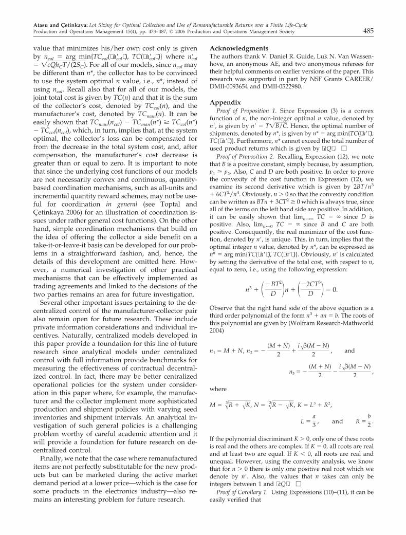
Proof of Proposition 3. Computing the second derivative ofTC� with respect to n we have (2BT)/n3 � (6CT2)/n4. Sincen � 0, for TC� to be convex, we need BTn � 3CT2 � 0, @n � 0.Using this inequality, as well as checking limn30� TC� andlimn3�� TC�, we have the results summarized in Table 3.

Observe that, if B � 0 and C � 0, then TC� is strictlyconcave so that the optimal n can be realized at the bound-aries of the feasible region; namely, either n* � 1 or n* � cQ . On the other hand, if we have B � 0 and C � 0, thenthe problem becomes a convex optimization problem forwhich the optimal solution is computed using the methoddeveloped for Special Case 2. That is, as suggested by Prop-osition 2, n* is given by Expression (15) where n� is theunique positive real root of the first derivative of TC�. Inother cases, i.e., (B 0, C � 0) and (B � 0, C 0), althoughwe cannot guarantee a single positive real root for the firstderivative of TC�, the optimal solution can be computedeasily as outlined in the last item of the proposition. Thiscompletes the proof. �

Proof of Corollary 2. Using Expressions (13) and (24), wehave

2TC�

tt1�

2chM Q�PT � cQ�

PT2 � 0, and2TC�

tP

�2�1 � c�chMQ2

P2T�

2chMQ2�2ct � ct1�

P2T2 � 0.

Consequently, TC� is supermodular in t1 and P so that t* isdecreasing in t1 and P. The monotonicity of hC, p, SC, and SM

follow the analytical reasoning of our results for SpecialCase 2 with the same conclusions. �

ReferencesAkcalı, E., M. A. Morse. 2004. Seeding strategies in remanufacturing.

Proceedings of the IIE Research Conference, Houston, Texas.Bras, B., M. W. McIntosh. 1999. Product, process and organizational

design for remanufacture—an overview of research. Roboticsand Computer Integrated Manufacturing 15 167–178.

Europa-Environment, “Waste”. 2005. http://europa.eu.int/comm/environment/waste/index.htm.

Fleischmann, M., J. Bloemhof-Ruwaard, R. Dekker, E. v.d. Laan, J. v.Nunen, L. N. Van Wassenhove. 1997. Quantitative models forreverse logistics: A review. European Journal of Operations Re-search 103 1–17.

Geyer, R., L. N. Van Wassenhove, A. Atasu. The impact of limited

component durability and finite life cycles on remanufacturingprofit, forthcoming in Management Science, 2006.

Guide, V. D. R., V. Jayaraman, R. Srivastava. 1999. Productionplanning and control for remanufacturing: A state-of-the-artsurvey. Robotics and Computer Integrated Manufacturing 15 221–230.

Guide, V. D. R. 2000. Production planning and control for remanu-facturing: Industry practice and research needs. Journal of Op-erations Management 18 467–483.

Guide, V. D. R., L. N. Van Wassenhove. 2004. Business aspects ofclosed loop supply chains. INSEAD Working Paper.

Guide V. D. R. Jr., G. C. Souza, L. N. Van Wassenhove, J. D.Blackburn. 2006. Management Science. 52(8) 1200–1244.

Haynsworth, H., R. Lyons. 1987. Remanufacturing by design, themissing link. Production and Inventory Management 28 24–29.

Hill, R. M. 1997. The single-vendor single-buyer integrated produc-tion-inventory model with a generalized policy. European Jour-nal of Operational Research 37 493–499.

Hill, R. M. 1999. The Optimal production and shipment policy forthe single-vendor single-buyer integrated production inventoryproblem. International Journal of Production Research 97 2463–2475.

Inderfurth, K., R. H. Teunter. 2001. Production planning and controlof closed-loop supply chains. Erasmus University Rotterdam,Econometric Institute Report 241.

Krumwiede, D. W., C. Sheu. 2002. A model for reverse logisticsentry by third party providers. Omega 30 325–333.

Lebreton, B., A. Tuma. 2003. Evaluating component recycling strat-egies. In Logistik Management—Prozesse, Systeme, Ausbildung,Spengler, T., S. Voss, H. Kopfer (eds.), Physica-Verlag, Heidel-berg, 333–347.

Lund, R. 1984. Remanufacturing. Technology Review 87 19–29.Muckstadt, J. A., R. O. Roundy. 1993. Analysis of multistage pro-

duction systems. In Logistics of Production and Inventory, Graves,S. C., A. H. G. Rinnooy Kan, P. H. Zipkin (eds.), Handbooks inOperations Research and Management Science, North Holland,Amsterdam, 59–131.

Paton, B. 1994. Market considerations in the reuse of electronicsproducts. IEEE International Symposium on Electronics andEnvironment, New York, New York, 115–117.

Rose, M. C., K. A. Beiter, K. Ishii, K. Masui. 1998. Characterizationof product end of life strategies to enhance recyclability. Pro-ceedings of DETC ’98, ASME Design for Manufacturing Sym-posium, Atlanta, Georgia.

Rose, M. C. 2001. Design for environment: A method for formulatingproduct end-of-life strategies. Ph.D Thesis, Stanford University,Department of Mechanical Engineering, Stanford, California.

RWorld. 2005. Direct sales franchise BM. http://www.rworld.ca/franchise_directsale_bus_model.asp.

Savaskan R. C., S. Bhattacharya, L. N. Van Wassenhove. 2004.Closed-loop supply chains with product remanufacturing.Management Science 50 325–333.

Thierry, M., M. Solomon, J. v. Nunen, L. N. Van Wassenhove. 1995.Strategic issues in product recovery management. CaliforniaManagement Review 37 114–135.

Toptal A. and S. Cetinkaya. 2005. Naval Research Logistics, Vol. 53(5),397–417.

Toptal, A., S. Cetinkaya. 2005. Contractual agreements for coordi-nation and vendor-managed delivery under explicit transpor-tation considerations. accepted for publication in Naval Re-search Logistics subject to minor revision.

Wolfram Research-Mathworld. 2004. Cubic Equation. http://math-world.wolfram.com/CubicEquation.html.

Viswanathan, S. 1998. Optimal strategy for integrated vendor-buyerinventory model. European J. of Operational Research 105 38–42.

Table 3 Main Model/Properties of bditTC�.

B C Convex if Concave if

�0 �0 Always Never�0 �0 n � � 3CT/B n � 3CT/B�0 �0 n � � 3CT/B n � � 3CT/B�0 �0 Never Always


Documents

PRODUCTION AND OPERATIONS MANAGEMENTaatasu3/index_files/AC06.pdf · PRODUCTION AND OPERATIONS MANAGEMENT POMS Vol. 15, No. 4, Winter 2006, pp. 473–487 ... 474 Production and Operations