PRODUCTION AND COST ANALYSIS OF A

SKYLINE CABLE LOGGING SYSTEM

OPERATING IN AN

UNEVEN-AGE MANAGEMENT PRESCRIPTION

A Paper Submitted to

Department of Forest Engineering

College of Forestry

Oregon State University

Corvallis, Oregon 97331

In Partial Fulfillment of the Requirements for the Degree of

Master of Forestry

Steven Alarid

July 2, 1993

APPROVED:

Dr. Loren D. Kellogg, Majo ProfessorForest Engineering

Dr. William A. Atkinson, Department HeadForest Engineering

Paper presented to graduate conunittee June 14, 1993

ACOWLEDGEMENTS

This project was completed as the result of many

individuals' efforts. I would like to express my appreciation tothose whose contributions have made this work possible.

The timber sale which provided the subject of this study was

administered by Oregon State University (OSU) Research Forestpersonnel. Debbie Cummings, Pain Beebe, and Jeff Garver provided

valuable information and assistance throughout the project. Saleadministrator Nike Rector was particularly helpful infacilitating field research procedures with a minimum of

interference with the logging contractor.OSU Forest Engineering Department personnel were quite

helpful; Judy Brennemnan and her office staff provided graciousadministrative support, and department head Dr. Bill Atkinsontsdoor was open for friendly professional counsel. Research

Assistant Pete Bettinger provided essential help and expertise inestablishing data collection and analysis methods and standards,performing field observations and data acquisition, and advisingon presentation of results.

The logging contractor, I'lore Logs, Inc., of Foster, OR, andcutting sub-contractor, Wischnofske Timber Falling, Inc., ofPhilomath, OR were cooperative and provided much insight ofexperience to this project.

Major professor Dr. Loren Kellogg contributed consistent and

much-appreciated guidance, advise, and motivation from beginningto end. Other coitunittee members Dr. Eldon Olsen and Dr. Bill

Emmingham offered excellent review and input in all phases of the

project, as well. Special thanks go to Dr. John Sessions for

joining the committee for the final oral examination.

My fiancee, and now my wife, my lovely Sherrie deserves more

than thanks for her cooperation, patience, and understanding

while I labored on this project throughout our engagement. Her

consistent encouragement often renewed and refreshed my resolve.

Finally, I would like to acknowledge and thank Almighty God

for Providential guidance in undertaking and completing this

work.

"Unless the Lord builds the house, he who builds labors in

vain." -King Solomon

1].

ABSTRACT OP THE PAPER OP

STEVEN ALRID

for the degree of Master of Forestry in Forest Engineeringpresented June 14, 1993.Title: Production and Cost Analysis of a Skyline Cable YardingSystem OperatincT in an Uneven-Age Management Prescription

Abstract approved: D.

Loren D. Kellogg

Forest managers in recent years have begun to re-examine thepossibilities of using uneven-age silvicultural systems in theOregon Coast Range. This increasing interest is being driven by avariety of forest resource nianagement concerns, including wildlifehabitat diversity, visual aesthetics, and long-term sustainedyield. In an effort to begin systematic exploration of coastaluneven-age silvicultural techniques, Oregon State University (OStJ)

researchers have established a demonstration site at Forest Peak onOSU's Dunn Forest.

This case study involving a single treatment at a single sitereports on the design, performance, and cost of the skyline loggingoperation during Septeither and October 1992 which was designed toachieve the goals of an uneven-age management prescription preparedby OSU silvicultural and wildlife specialists. The operationharvested 13.9 MBF of 23-inch average dbh Douglas-fir and grand firtimber.

The study tracked the time spent in planning and laying outthe logging system. Field and office planning and layout

procedures took 93.75 hours to conplete at a cost of $6.47/MBF.

The project also involved detailed time studies and shift-

level analyses of both the felling/bucking and the yarding phases

of the logging operation. A two-nan felling crew produced 6.44

MBF/Hr at a cost of $1O.44/MBF. Cutting cycle time averaged 9.22

minutes per tree, with nixnther of logs per tree, cutting method

(wedges or no wedges), percent ground slope, and base dianeter the

most influential factors affecting cutting cycle time.

The six-man yarding crew using a Thunderbird TTY5O yarder and

small Danebo MSP carriage yarded 4.7 MBF/Hr at a cost of

$58.51/MBF. Yarding cycle time averaged 5.73 minutes per turn,

with corridor yarding distance, lateral yarding distance, choker

setting method (pre-set or hot-set), and number of logs per turn

the most influential factors affecting yrding cycle time.

The six-man crew plus the hook tender averaged 1.82 hours for

each change of yarding corridors. Corridor changes involved moving

all rigging from one corridor to the next and repositioning the

yarder if necessary. The hook tender alone spent an additional

1.31 hours per corridor pre-rigging tail trees, anchors, etc.

Total logging cost including planning and layout, felling and

bucking, yarding, loading, and equipment move-in was $104.03/MBF.

ThBLE OP CONTENTS

INTRODUCTION 1

PURPOSE OF THE STUDY 1

SITE DESCRIPTION 3

Site Physical Conditions 3

Stand History and Structure 3

Silvicultura]. Treatnent 5

LITERATURE REVIEW 7

Logging Methods 7

Logging Planning 8

Residual Stand Damage 9

Logging Methods Summary 11

Logging Production and Cost Studies 13

LOGGING OPERATIONS OVERVIEW 19

Felling and Bucking 19

Yarding 20

Loading 21

STUDY METHODS 22

Initial Entry Logging Planning and Layout 22

Logging System Performance, Production, and Costs . . 24

Felling and Bucking Detailed Tine Study. 25

Felling/Bucking Shift-Level Analysis 28

Yarding Detailed Time Study 29

Yarding and Loading Shift-Level Analysis 31

Corridor Rigging Time Study. 32

iii

RESULTS 34

Unit Volume Production 34

Planning and Layout 35

Felling Time Study 37

Detailed Tinie Study 37

Felling and Bucking Regression Model 39

Felling and Bucking Production Rates and Costs . 40

Yarding and Loading Study 41

Detailed Delay Time Study 41

Road Change Time Study 42

Delay-Free Yarding Cycle Time Regression Model . 43

Yarding Production and Costs 44

Loading Production and Costs 44

Move-in Costs 45

Total Logging Production Cost 46

DISCUSSION 47

Production and Cost Comparisons 47

Planning and Layout 47

Felling and Bucking 49

Yarding Production and Costs 50

Total Cost Summary 51

Summary Conclusions 52

Other Considerations 54

Future Research Needs 55

REFERENCES 57

iv

APPENDIX A: RESEARCH METHODS LITERATURE 60

Time Study Techniques 60

Detailed Time Studies (Stopwatch Studies) 62

APPENDIX B: PRE- AND POST-HARVEST STAND INVENTORIES 68

APPENDIX C: LOGGING PLAN 87

APPENDIX D: REGRESSION ANALYSIS DOCUMENTATION 104

APPENDIX E: OWNING AND OPERATING COST CALCUlATIONS 111

V

LIST OP TABLES

Table 1. Pre- and Post-Harvest Stand Conditions 6

Table 2. Volume (MBF) produced from Forest Peak site. . . 35

Table 3. Planning and Layout Production and Cost. 36

Table 4. Felling cycle time elements (minutes). 38

Table 5. Felling and Bucking Delay-Free Regression Model. 40

Table 6. Summary statistics for felling and bucking

variables 40

Table 7. Suimnary of Felling and Bucking Production and

Costs 41

Table 8. Regression Model for Delay-Free Yarding Cycle

Time. 44

Table 9. Suiiunary statistics for yarding variables 44

Table 10. Summary of Yarding Production and Costs. 45

Table 11. Loading Production and Costs 45

Table 12. Move-In Costs ($). 46

Table 13. Total Logging Production Cost ($/MBF). 46

Table 14. Planning and Layout Time and Cost Comparisons . . 48

Table 15. Felling and Bucking Production and Cost

Comparisons 50

Table 16. Yarding Production and Cost Comparison 51

Table 17. Total Cost Comparison, 1993 dollars. si

vi

LIST OF FIGURES

Figure 1. Feller Cycle Time Elements 37

Figure 2. Bucker Cycle Time Elements 37

Figure 3. Averaged Felling Cycle Time Elements 37

Figure 4. Felling Delay Time Elements 39

Figure 5. Yarding Cycle Time Elements 42

Figure 6. Yarding Delay Time Elements 42

Figure 7. Road Change Time Elements 43

vii

INTRODUCTION

Forest managers in recent years have begun to re-examine thepossibilities of using uneven-age silvicultural systenis in theOregon Coast Range. For example, the currently proposedMacDonald/Dunn Forest Plan (OSU 1992) allocates approximately

one-third of the Forest's timber management area to uneven-ageprescriptions. Also, the USDA Forest Service's current eniphasison Ecosystem Managentent is bringing uneven-age nianagentent into

increasingly serious consideration. This increasing interest isbeing driven by a variety of forest resource management concerns,including wildlife habitat diversity, visual aesthetics, and

long-term sustained yield. In an effort to begin systematicexploration of coastal uneven-age silvicultural techniques,Oregon State University (OSU) researchers have established a

demonstration site at Forest Peak on OSU's Dunn Forest.

PURPOSE OP THE STUDY

While uneven-age silviculture is an established practice inother locations, little has been attempted in the Coast Range.

Fire history of the coastal region has resulted in an almostexclusively even-age natural forest, so there are few naturalexamples of uneven-age structure. Economics, terrain, andtechnology have limited most Coast Range timber management toclearcut harvesting and subsequent even-age plantationmanagement. In order to niake informed decisions about suitable

silvicultural systems for achieving a widening variety of

1

objectives, planners and managers must be able to determine

logging feasibility and costs.

This case study involving a single treatment at a single

site reports on the design, performance, and cost of the skyline

logging operation during September and October 1992 which was

designed to achieve the goals of an uneven-age management

prescription prepared by OSU silvicultural and wildlife

specialists.

Specific goals of the study are:

Determine prescription-specific harvest unit

planning and layout requirements and costs for the

current entry.

Determine cycle times, detailed time elements of

each cycle, predictive delay-free cycle time

equations, volume production rates, and costs for

the following components of the harvesting

operation:

- felling and bucking

- yarding

- loading

- yarding corridor changes

Compare the production and cost results of this

study with results of other studies in similar

stand conditions using similar logging systems.

2

SITE DESCRIPTION

Site Physical Conditions

The 22.8-acre study site is located within OSU's Dunn Forest

in section 22, NW 1/4, T.10 S., R.5 W., Willamette baseline and

meridian, at the crest of Forest Peak on the Willamette River

Valley fringe on the eastern slope of the Oregon Coast Range.

Elevation ranges from 860 to 1480 feet, averaging 1170 feet.

Aspect ranges from southeast to west, averaging 201 degrees

azimuth. Slopes range from 25 to 47 percent, averaging 38

percent. Soil types are 41 percent Price, 31 percent Ritner, 21

percent Witzel, and 7 percent others. Rainfall averages

approximately 45 inches per year.

The combination of south to west aspect and the position on

a well-drained upper slope make this a ttdrytt site for the Coast

Range. Understory vegetation consists primarily of Oregon-grape

(Berberis nervosa), poison-oak (Ruus parviflorus), vinemaple

(Acer circunatuin), salal (Gaultherja shallon), several

blackberries (Rubus spp.), and various grasses and herbs. This

plant association is typical of sites with high moisture stress

during dry periods. It is considered to be low competition with

conifer seedlings.

Forest Peak is a prominent local landmark, and the study

site is clearly visible from surrounding rural roads and

neighborhoods.

3

Stand History and StructureThe stand of 75 percent Douglas-fir (Pseudotsuga nienzeisii),

14 percent grand fir (Abies grandis), and 1]. percent Oregon whiteoak (Quercus garryanna) and bigleaf maple (Acer inacrophylla) hadthree basic coniponents: 1) 1-2 trees per acre (TPA) of largeDouglas-fir "wolf" trees 200 years of age or more and 40 inchesdiameter at breast height (dbh) or greater; 2) 60 TPA beforeharvest of 120-year-old Douglas-fir and grand fir with mean dbh

of 22.7 inches; 3) 699 TPA before harvest of Douglas-fir, grandfir, and bigleaf maple less than 8 inches dbh.

The largest coniponent is the 120-year-old age class with 60

TPA and mean dbh of 22.7 inches before the cable entry. The

origin of this stand propabaly dates to the period in historywhen native peoples and early Willamette Valley settlers ended

their practice of regularly broadcast burning the Coast Rangefoothills. This stand component was naturally seeded by the few

large parent trees which still remain scattered throughout thestand.

A commercial thinning in 1968 removed approximately 12

MBF/acre. The logging was accomplished using a crawler tractoron designated skid trails. This thinning opened the canopy andexposed mineral soil by scarification, allowing direct sunlightto reach the understory and forest floor and creating the baresoil spots needed for natural Douglas-fir regeneration.

The dry site/low coiupetition conditions coupled with thethinning "site preparation" in 1968 resulted in the establishment

4

of the naturally-regenereted understory of mixed Douglas-fir,

grand fir, and bigleaf maple at 699 TPA less than 8 inches dbh

before harvest in 1992.

This type of understory density is not conmon in the Coast

Range. Most of the Coast Range forest canopy is closed,

p-reventing widespread establishment of even shade-tolerant tree

species. In places where the canopy has opened due to

catastrophic events or management operations, understory

vegetation quickly dominates most sites. 'Forest Peak was chosen

for an uneven-age management demonstration because it typifies

the limited areas in the Coast Range where site-specific

conditions could allow establishment of a multi-storied conifer

stand structure.

Silvicultura]. Treatment

The objective of the uneven-age management prescription is

to establish a conifer stand with a distribution of size classes

from seedling to mature in appropriate proportions. Since the

stand was initially an even-age structure, the stand will require

several harvest entries - each entry removing a portion of the

harvestable stems per acre - before reaching the future desired

multi-story structure. The 1968 tractor thinning was actually

the first entry of this conversion period, although at the time

there was no known intention of managing on an uneven-age basis.

The cable harvest operation of September/October 1992 which was

the subject of this study constituted the second entry of the

5

conversion period.

The silvicultural prescription originally called for

removing approximately 40 percent of the stems from the 120-year-

old overstory and protecting the 699 TPA understory from damage

as much as possible. Table ]. describes actual stand conditions

before and after the harvest operation. Complete pre- and post-

harvest inventories, including growth information, are included

in Appendix B. The increase in post-harvest hardwood 0"-4" TPA

is most likely due to sampling error; pre- and post-harvest

inventories were taken only one year apart. The decrease in 4"-

8" conifers was due mostly to timber felling damage and clearing.

6

Table 1. Pre- andClass and

Pre-Harvest, 199].

Post-Harvest Stand Conditions by DiameterSpecies, from OSU stand exams.

Trees/Acre Basal Area/Acre0fl_4t1 Sq.Ft., >8" dbh

D-fir 275 6 45 196grand fir 161 40 8 6hardwoods 206 12 7 4TOTAL 642 57 60 206

Post-Harvest, 1992D-fir 232 0 27 128grand fir 92 29 7 4hardwoods 252 12 7 4TOTAL 573 40 43 136

Change -11% -30% -28% -34%

LITERATURE REVIEW

Logging Methods

There is little published literature documenting cable

logging systems in uneven-age prescriptions. However, much

research has been recorded in shelterwood cable logging, using

cable techniques which are applicable to this project. The

Forest Peak stand being managed for uneven-age structure was

essentially a two-story stand at the beginning of this study. It

was a thinned mature even-age stand with an advanced regeneration

understory. The cable logging entry which was the subject of

this study resenibled certain elements of both a shelterwood

initial cut and an overstory removal.

Shelterwood management is an even-age silvicultural system

with harvest and regeneration accomplished in a two-stage (or

sometimes three-stage) process. The first stage, called the

initial or shelterwood cut, removes most of the stems in a stand.

Approximately 8-15 trees per acre are left standing to provide

shading and sometimes a seed source for the even-age stand being

regenerated. Seedlings are planted or seeded naturally beneath

the shelterwood overstory. When the regeneration becomes

established the second stage, or overstory removal, is

accomplished. This stage removes any remaining stems not

required as permanent leave trees.

Shelterwood management requires protection of residual crop

trees during the initial cut and protection of regeneration

during the overstory removal. Uneven-age management requires

7

protection of both the next cycle's crop trees and regeneration

in the same entry.

Several previous studies have described mechanical methods

for protecting the residual stand in shelterwood operations using

cable systens. These techniques, which are also applicable to

protecting residual trees in an uneven-age prescription, are

summarized below.

Logqinq Planning

Because protection of the residual stand is a major objective of

uneven-age logging, planners ntust consider how many trees can be

felled at each entry while maintaining adequate undamaged

stocking in the desired size classes. Based on Paine and Hann's

(1982) work with crown dimensions, Mann (1985b) simulated how

much ground surface area felled trees of various sizes occupy.

For example, 14 trees per acre (TPA) of 30 inch diameter at

breast height (dbh), 150 foot height, and 44 foot crown width

occupy 60 percent of the ground surface area when felled. While

more research will be needed to better deter'mjne how much stand

damage is caused by various cut/leave intensities, Mann's

simulation provides a reference point for planning purposes.

In the same article, Mann pointed out the need for

estimating the locations of future skyline corridors and leaving

trees which can serve as lift or anchor trees. Trees used as

tail spars or intermediate supports in the current entry may have

weakened root systems and may die by the next entry. This means

8

yarding corridor locations will potentially change to find

healthy lift trees in the next entry. Logging planners must be

sure silvicultural prescriptions and marking guides account for

this logging requirement.

Residual Stand Damage

Logging damage to both existing regeneration and residual

mature trees has been studied in various regions and forest

types. Tesch, et al.(1986), working in a southern Oregon mixed

Ponderosa pine/Douglas-fir shelterwood overstory removal, found

22 percent seedling mortality from felling and 28 percent

mortality from cable yarding among seedlings surviving felling,

or a total of 4]. percent seedling mortality from logging

operations. Tail lift trees were not used, resulting in some

ground-lead yarding. The overstory consisted of approximately 20

TPA with average dbh of 24 inches. Seedling mortality was lowest

in the 60-100 cm (23.6-39.3 inch) height range. Damage was

highest directly within yarding corridors and adjacent to

corridors with greater than 45 percent cross slope. Tesch

recommended spacing yarding corridors as widely as possible,

minimizing nuniber of corridors per landing, and not yarding on

corridors with greater than 45 percent cross slope.

Youngblood (1990) compared Alaska white spruce seedling

damage from shelterwood overstory removal using a rubber-tired

skidder and a skyline cable system. The overstory stand

conditions were 28-56 cm (11-22 inch) dbh, 29-35 m (95-115 feet)

9

height, and 10.3-12.7 ft2 basal area. Cable corridors were 38 m(125 feet) apart with tail lift trees to improve deflection and

log control. Cable yarding resulted in 15 percent mortalityamong seedlings, with the lowest mortality in the 70-90 cm (27.6-35.4 inch) height range. Ground skidding resulted in 45 percentmortality

Benson and Gonsior (1981) measured damage to marked leave

trees after an initial shelterwood cut in two Douglas-fir/westernlarch stands in Montana. Both running skyline and live skylinesystems were used to yard the units. Stand 1 averaged 109 TPA

greater than 7 inches (17.8 cm) dbh, and Stand 2 averaged 147 TPA

greater than 7 inches (17.8 cm) dbh. Both units were leave-treemarked to retain half the volume of trees greater than 7 inches(17.8 cm) dbh. Four utilization standards were conipared fordifferences in percent mortality and percent undamaged:

All uinarked trees down to 5 inch (12.7 cm) dbh were

cut. All material down to 8 feet long by 3 inches topdiameter was yarded. Residue was broadcast burned.Umarked trees down to 7 inch (17.8 cm) dbh were cut.Materials down to 6 inch top diameter were yarded.Residue was burned.

Unmarked trees down to 1 inch (2.5 cm) dbh were cut andrenioved. Residue was not burned.

Unmarked trees down to 7 inch (17.8 cm) dbh were cut.Materials down to 8 feet long by 3 inches top diameterwere yarded. Residue was not burned.

10

After removal of approximately half the TPA and basal area

in both stands, mortality and undamaged trees varied little

between treatments within a Stand. In Stand 1, an average of 22

percent of marked leave trees were killed, while 40 percent were

undamaged. In Stand 2, an average of 25 percent were killed,

while 29 percent were undamaged. Average overall mortality was

23 percent, and average overall undamaged was 34 percent. Benson

and Gonsior recommended accounting for expected mortality by

marking enough leave trees to compensate for trees killed during

felling and yarding.

Logging Methods Summary

The results of these studies reveal important information to

be considered when developing both logging plans and

silvicultural prescriptions for uneven-age management. Logging

plans must provide for protection of the residual stand as much

as possible as sununarized by Mann (1985a):

felling trees to lead

spacing yarding corridors to minimize damage to

residual trees, either by reducing lateral yarding

distances for improved log control, or by increasing

lateral yarding distances to reduce the number of main

corridors. This decision is dependent upon site-

specific conditions.

positioning yarding corridors perpendicular to the

contour; not yarding on steep (>45%) cross slopes

11

using a carriage which can hold its position on the

skyline during lateral inhaul and not starting corridor

irthaul until the log has actually reached the corridor.

providing at least single-end log suspension for better

log control during yarding

minimizing lateral cable deflection by using rub trees

which are felled and yarded last

minimizing the number of corridors per landing, using

parallel settings if possible

clearly conuuunicating residual stand protection

objectives to the logging operators.

Silvicultural prescriptions must provide means for arriving

at the desired stand structure within the limitations of

available logging technology. Factors to be considered in

developing a prescription and marking guide are:

compensating for anticipated logging damage and

mortality to the residual stand - both seedlings and

mature trees - when prescribing residual stand

structure

allowing sufficient numbers of leave trees in suitable

locations for future tail spars and intermediate

supports as necessary

considering the impacts of residual stand structure on

logging feasibility in the next cycle.

12

Logging Production and Cost Studies

While documentation of skyline logging systems operating in

uneven-age prescriptions is rare, production and cost research in

other partial-cut systems is not uncommon. Several pertinent

studies have been published describing production and cost data

collection and data analysis for a variety of skyline/partial-cut

combinat ions.

Kellogg, Pilkerton, and Edwards (1991) examined skyline and

ground skidding systems in three harvest prescriptions in mature

Douglas-fir. The cutting prescriptions were clearcut, two-story

even-aged (shelterwood), and half-acre group selection patch

cuts. A Thunderbird TTY 50 tracked mobile yarder with a Danebo

MSP mechanical slack-pulling carriage rigged in a standing

skyline slackline configuration was used for cable yarding in

this project. Skyline roads were rigged as single spans, with

some requiring intermediate supports or tail trees.

Two types of data were collected:

Logging planning and unit layout time for each

management prescription type.

Shift-level time and volume production data for felling

and yarding for each management prescription type.

Logging planning for clearcuts involved unit reconnaissance,

flagging landings, surveying skyline ground profiles, performing

payload analyses, marking leave trees, and preparing maps.

Logging planning on the two-story and patch cut units involved

more time than planning a clearcut, due to the increased time

13

required to select and flag designated skyline corridors and lift

trees, as well as preparing more detailed maps. Total planning

and layout time was tracked for each prescription. Time results

for each prescription were reported in man-hours per MBF volume

removed and cost was reported in dollars per MBF removed. Both

time and cost for the cable system were approximately six times

higher for two-story and group selection than for clearcutting.

The felling and yarding time studies followed the shift-

level model described in Olsen and Kellogg (1983), sulmnarized in

Appendix A. Felling crews consisted of ten cutters, each working

equal time in all three prescriptions. Production and cost

results for each prescription were reported in units of gross MBF

felled per shift hour and dollars per MBF. Felling production

was highest for group selection and lowest for two-story.

Conversely, cost was lowest for group selection and highest for

two-story.

Cable yarding crew consisted of eight men on the site.

Production results were again reported in units of MBF volume per

yarder shift hour, and costs were reported in units of dollars

per MBF yarded. Two-story and group selection yarding production

were approximately 80 percent of clearcut production. Costs were

approximately 22 percent higher than clearcut.

Total cost figures for each prescription were also

calculated, including layout, felling, and yarding. Total cost

for both two-story and group selection were approximately 24

percent higher than clearcutting.

14

Edwards (1992) examined a skyline system operating in five

different group selection prescriptions. The study was conducted

in stands of approxiamtely 100-year-old Douglas-fir very similar

to the stand being treated in the current Forest Peak study. For

this project, a Thunderbird TMY 70 mobile yarder with a Danebo

S-35 Drumlock mechanical slack-pulling carriage was rigged in a

standing skyline with haulback configuration. The six

prescriptions were:

Clearcut - served as a baseline prescription against

which other treatments were compared.

Strip cuts removing approximately one-third of the unit

area in parallel rectangular strips.

0.5-acre patch cuts in fan settings removing one-third

of the unit area in rectangular or polygonal patches.

1.5-acre patch cuts in fan settings removing one-third

of the unit area in rectangular or polygonal patches.

2.5-acre wedge cuts in fan settings removing one-third

of the unit area in rectangular or polygonal patches.

0.5-acre patch cuts in parallel settings removing one-

third of the unit area in rectangular or polygonal

patches.

Three types of production data were collected: logging planning

and layout time, shift-level time and volume production, and

detailed stopwatch study information for felling, yarding, and

cable road changes. A hand-held field data recorder with a

15

commercial time study software package was used for collection ofdetailed tiire information.

Planning and layout results revealed large increases in tiirefor all five alternative prescriptions. Planning and layout timewas measured in units of hours per acre. Increased times abovethe baseline of 1.69 hours/acre for clearcut ranged from 362percent for strip cuts to 690 percent for 0.5-acre patch cuts.

Felling results revealed only small differences in MBFproduction per hour and cost per MBF for all six treatnients.Clearcut production was 4.5 MBF/hour and cost was $8.56/MBF. No

treatment varied more than 3 percent from clearcut felling ineither production or cost.

Yarding results similarly showed little difference among the

six treatments. Clearcut yarding production was 7.2 MBF/hour andcost was $48.96/MBF. None of the alternative treatments variedmore than 5 percent from this baseline.

Yarding corridor and landing change time results did revealmajor differences in treatments. Clearcut results were:

Average corridor/road change time = 1.53 hoursNo. changes per 25 acre unit = 12

Cost per road change ($/MBF) = 9.16

The highest average change times were 3.67 hours for the 0.5-acreparallel set patch cuts and 2.96 hours for the strip treatment.These parallel setting treatments required moving the yarder foreach corridor change. The wedge treatment required only 1.72hours per change, the lowest of the five alternatives.

16

While the clearcut change time was the lowest, the number of

changes per unit area was the highest of all the treatments.

Others required from 2 to 9 changes per unit area. The wedge

prescription only required 2 road chages per 25 acres, resulting

in a total cost of $4.36 per change, 52 percent below

clearcutting. The 0.5-acre fan setting patch cuts cost 108

percent more than clearcuts.

Total volume production in units of MBF per hour was

calculated for scheduled hours, including all road changes and

delays. Clearcut production was 6.1 MBF/Hr. Highest production

was on the wedge prescription, at 6.8 MBF/Hr, and lowest

production was on the 0.5-are fan setting patch cuts, at 5.7

MBF/Hr.

Total costs ranged from a low of $63.58/MBF for clearcut to

$80.11/MBF for 0.5-acre fan set patch cuts, a 26 percent

difference. The wedge treatment was closest to clearcut at

$65.71.

Both of the shift-level analyses reviewed here have

applications for the current Forest Peak study. Both studies

were conducted on OSU's McDonald Forest in stand conditions very

similar to the stand treated at Forest Peak. The yarding

equipment and crew size in Kellogg, Pilkerton, and Edwards (1991)

were identical to those used at Forest Peak, making it possible

to directly compare results of the two yarding studies. While

the yarder and carriage used in Edwards 1992 study differed from

Forest Peak, it would be possible to make an interesting

17

comparison of relative production rates in the various nianagement

prescriptions.

18

LOGGING OPERATIONS OVERVIEW

Felling and Bucking

A complete logging plan, including profile analyses and

payload analyses, is located in Appendix C. This section is a

qualitative overview of the several phases of the logging

operation which was the subject of this study.

The felling and bucking phase of the logging was

accomplished by two cutters working together as a pair. The lead

cutter, or feller, had primary responsibility for the felling of

the trees. He determined which tree would be felled next and

where each tree would be laid. He made most of the face cuts and

back cuts. He also helped with a portion of the .bucking and

linthing. The second cutter, or bucker, assisted with the felling

(placing wedges, spotting, etc.) but was primarily responsible

for bucking and linthing the tree once it was on the ground.

While the bucker was bucking the felled tree, the feller would

usually select and move to the next tree to be felled and begin

making his cuts. When the bucker finished bucking his tree into

logs, he would proceed to the next tree to assist with the

felling. Each cutter occaisionally took over the other's duties

when there was a mechanical breakdown or the other cutter was

occupied at another task.

Each cutter used a Stihl 064 chainsaw with a 36-inch bar.

Each carried his own fuel and oil containers, basic tool kit,

replacement chains, wedges, single-bit axe, and water.

The bucker kept daily records of the number of trees felled,

19

nuniber of logs bucked from each tree, and total shift hours

worked for the crew of 2.

Yarding

Yarding was accomplished using a Thunderbird TTY-50 track-

mounted mobile yarder. It was rigged in a standing skyline

configuration with a haulback using a Danebo MSP (small model)

mechanical slack-pulling carriage.

The yarding required seven full-time men plus occaisional

visits by the company owner. The yarding crew consisted of the

yarder operator and two chasers on the landing, and a rigging

slinger and two choker setters in the brush.

The hook tender, the seventh crew meniber, only worked at

pre-rigging yarding corridors and supervising road changes

(moving the skyline and other rigging to the next corridor when

one corridor was finished). Pre-rigging involved selecting and

preparing tailholds for the skyline, rigging pre-selected tail

trees with the necessary blocks and guylines, and rigging pre-

selected intermediate support trees with blocks and guylines.

Skyline tail holds were either stumps in adjacent units or heavy

equipment (an old crawler tractor) when suitable stumps were not

available. Because the cable system on this site required tail

trees on all all but one corridor, and one corridor required an

intermediate support, the hook tender worked full time at pre-

rigging the next corridor for yarding. The original logging plan

in Appendix C called for intermediate supports on corridors 9-11,

20

but the loggers only used them on corridor 10.

Loading

The loader was a John Deere 892D-LC, a track-mounted,

hydraulic heel-boom grapple loader. It was operated by a single

crew member in addition to the seven men on the yarding crew.

Because the yarding production was low in the partial cut with

short roads and relatively frequent road changes, the loader

could load trucks faster than the yarder could yard logs in.

However, the loader operator had no other operational duties than

to run the loader, even during idle periods. The operator did

keep daily records of number of logs yarded, number of trucks

loaded, and total crew shift hours for both the yarder and the

loader.

21

STUDY METHODS

This study was intended to document the planning and

implementation of a skyline logging entry in an uneven-age

management prescription. Logging design, field layout, and

logging operations were carried out as part of an actual timber

sale process on OSU's Dunn Forest. Data was collected

observationally as the various work phases progressed through

their normal sequence. Because of the range of objectives of

this study, data was collected and analyzed using a variety of

methods. These methods are described below. All financial

calculations were based on 1993 dollars.

Initial Entry Logging Planning and Layout

Selected components of the planning and layout phase of

operations were tracked for the time spent in each activity.

Activities selected for observation in this study were those

which are common to all logging operations but potentially differ

in quality or quantity from other management prescriptions. This

information was used to determine sale prep time requirements and

costs on this site with this prescription. Some activities, such

as unit boundary layout or haul route design, were not unique to

this treatment and were not tracked.

A daily log of planning and layout activities was kept which

recorded the nunther of man hours spent in each of the individual

categories. Because problenis or changes did arise during logging

operations, planning and layout activities continued to some

22

extent throughout the project.

were:

Plannning and layout activities selected for observation

- Field reconnaissance. This was considered to be general

unit examination, note-taking, or similar field

observations. Not included were any of the specific field

tasks listed below. This phase was completed by the

principal researcher, OSU faculty researchers, the OSU

sale administrator, and two research assistants.

- Office Planning. This included map and inventory

analysis, preparation of documents, conferences, and any

other administrative or indoor activity directly related

to this timber sale. Not included were activities related

only to the study or any other activity which was not a

part of the normal timber sale process. This phase was

accomplished by the principal researcher.

- Ground Profile Surveying and Traversing. This included

time spent in the field taking survey measurements. This

phase was accomplished by the principl researcher and a

technical assistant.

- Logciing Plan Development. This included all profile and

payload analyses, cable system design, landing and

corridor design and location, and all other design

procedures contributing to the "paper" logging plan. This

was accomplished by the principal researcher.

- Landing and Yarding Corridor Layout. This included field

23

identification of landings, specific tail trees and/or

anchors, taking any necessary measurements, and flagging

the corridors from landing to tailhold. This phase was

accomplished by the principal researcher.

- Tree Marking. This was the field time it took the crew to

accomplish a cut-tree mark. This phase was accomplished

by seven OSU faculty researchers, the OSU sale

administrator, and the principal researcher.

Total planning and layout time was determined by summing the

hours in each of the listed categories. Unit cost was calculated

two ways - dollars per MBF and dollars per acre. Total cost was

determined by multiplying total hours by total cost per hour.

Unit costs were determined by dividing total cost by total volume

from scale tickets and by dividing total cost by total unit

acreage.

Logging System Performance, Production, and Costs

Tracking and reporting on the logging system involved

several data collection and analysis methods. Five time studies

were conducted: two tracked the detailed components of the

felling/bucking and the yarding operations. Two shift-level

analyses tracked daily equipment and personnel time for both the

felling/bucking and the yarding operations. Another tracked

gross time spent rigging the yarding corridors.

Volume production and costs were calculated for each

operation, using data from scale tickets and data collected as

24

described below.

Felling and Bucking Detailed Time Study.

Data from this time study was used to deteriuine an average

cutting cycle time for this project and to develop a predictive

equation for delay-free cycle time with the given stand

conditions and prescription.

The unit was felled by cutters working as a pair. The

felling and bucking time study tracked the time the pair of

cutters spent felling and bucking logs.

This operation was divided into its procedural components,

and each component was timed to the nearest decimninute (100th

minute) for each tree. Each cutter was tracked for the duration

of the felling and bucking operation which lasted eight days.

Three days of data collection were lost for a variety of reasons,

including incorrectly recorded data, researchers' schedule

conflicts, and an injury to the lead faller, forcing the other

cutter to finish the unit alone. The lead faller was timed with

a hand-held Husky Hunter field data recorder. The SIWORK3 time

data collection program was used. The second cutter, or bucker,

was timed by a second researcher with a stop watch and paper

spreadsheet. The stopwatch was used because there was only one

functional data recorder available. Timed components recorded

were:

- Travel and Preparation. This was the time spent between

the completion of bucking one tree to the beginning of

25

felling the next tree. This included any brush clearing,

sizing up, or felling of tress less than 4" diameter

needed to fell the next tree. Time began when the cutter

completed his final buck cut on one tree and headed for

the next tree.

- Felling. Time began when the saw blade touched the tree

to make the undercut or backcut. Time ended when the tree

hit the ground. Felling trees less than 4" diameter was

not timed.

- Bucking and Limbing. Time began when the tree hit the

ground and ended when the cutter completed his final buck

cut.

- Delays. Timed delays were recorded for:

Mechanical delays such as saw breakdowns, bar or

tuning adjustments, or fueling and oiling.

Personal delays such as lunch or rest breaks.

Procedural delays such as conferences with foreman

or administrator, stopping to help with another

task, bar hang-ups, etc.

Planning delays. This was the time spent

deterniining felling patterns, discussing how to

proceed with a task, etc. This usually occured at

the beginning of the day or the beginning of some

new portion of the work. This did not include

preparations for felling each individual tree.

Other miscellaneous delays.

26

Other information collected for each tree was:

- Merchantable/Non-merchantable. Non-merchantable conifers

were sometimes felled to clear corridors or to facilitate

felling the merchantable tree. All hardwood trees were

counted as non-merchantable. This was a 0/1 indicator

variable with 0 = non-merchantable and 1 = merchantable.

Felling any trees less than 4" diameter was recorded as

travel/preparation time.

- Inside Bark Butt Diameter. Average of two diameter

measurements taken at right angles to each other.

- Number of Logs Cut From Tree. Recorded for each cutter

separately.

- Buck Cuts. Number of buck cuts for each cutter, including

bucking out defects.

- Method. Denote which felling technique was used: 0 = no

wedges and 1 = wedges.

- Slope. Percent slope at the base of the tree.

- Tree Lay Slope. This was the percent slope of the fallen

tree from the stump in the direction of the fall. This

variable was included as an attempt to determine whether

the directional felling up or down the ground slope

required in this partial cut had an effect on felling

time.

Collected data were entered into a computer spreadsheet for

27

analysis. Cycle time elements were determined for each cutterseparately, and a crew time per tree was determined by averagingthe individual time elements. For example, if feller fellingtime = 2.69 minutes and bucker felling time = 2.01 minutes, thenaveraged crew felling time = 2.35 minutes. Another way of

describing this process is if each cutter spent 9 minutes totaltime per tree, then the averaged crew time per tree would be 9

minutes.

A predictive delay-free felling/bucking time equation was

developed using a step-wise regression analysis procedure. Thisequation described travel, felling, and bucking time per tree asa function of site and operational characteristics: buttdiameter, number of logs cut, number of buck cuts, fellingmethod, percent ground slope, and percent log lay slope.Equations were developed for each cutter seperately, and a

combined crew equation was developed by averaging the twoindividual equations.

Fellinq/Bucking Shift-Level Analysis

The cutting crew kept a daily record of their shift hours,number of trees felled, and number of logs cut per tree. Thisinformation was used to help determine production and costs forthe operation. Tree production was determined by dividing thetotal number of trees on the shift-level forms by the total 2-niancrew hours worked (2 nien working 8 hours each = 8 crew hours).

Volunie production was determined by dividing the number of logs

28

cut by the crew hours worked. Individual log volume was then

determined from the scale tickets by dividing total volume scaled

by total number of logs. Multiplying logs per hour by volume per

log yielded volume per hour for the felling/bucking operation.

Yarding Detailed Time Study

The yarding time study separated the yarding operation into

its procedural components, and each component was timed and

recorded. Data was collected using the Husky Hunter field data

recorder with the SIWORX3 time data collection program. Two

workers were required to collect the necessary information. One

worker followed the choker-setting crew to observe, while the

second worker remained at the landing to observe and record data.

The two were in contact by hand-held radio, so the one recording

information knew when activities at the other end of the line

began and ended. Timed components were:

- Outhaul. Time began when the carriage left the landing

and ended at the carriage stop signal.

- Lateral Outhaul. Time began with the carriage stop signal

and ended with the dropline stop signal.

- Hook. Time began with the dropline stop signal and ended

with the dropline ahead signal.

- Lateral Inhaul. Time began with the dropline ahead signal

and ended with the carriage ahead signal or when the turn

reached the corridor and was ready for inhaul.

- Inhaul. Time began with the carriage ahead signal or when

29

the turn reached the corridor and was ready for inhaul.

Time ended when the turn was landed.

- Unhook. Time began when the turn was landed and ended

when the carriage started back down the skyline.

- Delays. Delays will be recorded by the following

categories:

Rigging. Repair or adjust rigging, including

lines, chokers, blocks, anchors, and carriage.

Equipment. Repair or adjust equipment such as the

yarder or loader.

Personal delays such as lunch or rest breaks.

Procedural delays. This included a wide variety

of possible delays: landing problems, waiting for

other equipment, fueling, clearing obstacles, etc.

Repositioning. This included any rigging

repositioning, including choker resetting or

repositioning the carriage. This did not include

yarder repositioning associated with road changes.

Other miscellaneous.

Other recorded components (non-timed) were:

- Yarding Distance. Slope distance between the tower and

point where the carriage stopped, estimated to the nearest

ten feet. Trees or stumps were marked in fifty-foot

increments along the length of the corridor to aid in

estimating distance.

- Lateral Distance. Average distance measured perpendicular

30

to the corridor to the hooking point of the farthest login the turn, measured to the nearest five feet.

- Preset. Indicator variable (0/1) denoting whether chokerswere preset or hotset.

- Merch.. Number of merchantable logs in the turn.- Non-Merch. Number of non-iaerchantable logs in the turn.

All hardwoods were called non-merchantable, regardless oflog quality.

Collected data were downloaded to a personal coiaputer foranalysis with spreadsheet and statistical software. Yarding

cycle time eleiaents were determined by averaging the individualcycle components and suTnming theni for an average total cycle tiiaefor this site and prescription. A step-wise regression analysisprocess yielded a predictive equation which described delay-freetinie per yarding cycle as a function of the five non-timedoperational coniponents listed above.

Yardinci and Loadipg Shift-Level Analysis

The yarding and loading crews kept daily records of theirshift hours, number of logs yarded, and number of trucks loaded.This information was used to help determine production rates andcosts for the yarding and loading operations.

Yarding and loading production were determined by dividing

the total volunie froni the scale tickets by the total shift hourson the shift-level forms.

Yarding and loading owning and operating costs were

31

determined using the PACE program with cost and procedural

information froni several sources (USDA 1992, Edwards 1992,

Kellog, Olsen, and Hargrave 1986, and Miyata 1980). PACE is a

spreadsheet-driven program which utilizes user-supplied costinformation to calculate equipment ownership and operating costsin dollars per hour. PACE outputs for the yarding and loadingoperations are included in Appendix E.

Corridor Rigging Tinie Study.

Corridor rigging was divided into four phases. Tinies were

kept to the nearest niinute using a wristwatch, and data wasrecorded on a paper spreadsheet. Pre-rigging tinie was recordedby the hook tender and relayed to the researchers at the end ofeach shift. This collected information was used to calculateaverage road change times including pre-rigging.

The four tinied phases were:

- Pre-rigqing. This was the tinie the hooktender spentlaying out rigging in the next yarding corridor inpreparation for the next road change. The hooktender

sonietinies pre-rigged several corridors ahead, so it wasimportant to keep in close daily contact with hini toobtain accurate time data.

- Rig-down. Tinie began when the last turn in a corridor wasunhooked at the landing. Tasks included pulling in linesand guylines, renioving blocks or other anchor rigging,etc.

32

- Move or Reposition Yarder. Some judgement was required to

determine when this phase actually began. Rigging a new

guyline anchor stump would be part of yarder

repositioning, as would raising the yarder outriggers.

Moving or repositioning time began before actual yarder

movement, but required the researcher to determine the

beginning point for each move seperately. This phase did

not occur for all road changes since several corridors

could be yarded without changing xosition.

- Rig-up. Beginning time was again a subjective

determination. Generally rig-up began when the yarder was

set in place and lines were beginning to be pulled down

the corridor. However, support tree rig-up may start

earlier, so beginning time was judged for each corridor

seperately.

33

RESULTS

Unit Volume Production

Table 2 displays total volume and volume per acre cut from

the Forest Peak site. Total volume cut in thousands of board

feet (MBF) was determined from the log scale tickets. Saw log

scale was read directly from the tickets. Pulp logs were sold by

weight, so a conversion calculation was necessary. Pulp logs

weighed 105,300 lbs. delivered at the Coastal Fibre mill in

Willamina, OR. Pulp log volume was calculated using a conversion

ratio from Dilworth (1977) for 14-20 inch Douglas-fir logs of

12,770 lbs. per MBF.

Unit size of 22.8 acres was determined by OSU technicians by

digitizing the stereo plotter contour map of the unit.

Volume per acre was figures from pre- and post-harvest

inventories of the stand conducted by OSU Forests field

technicians were also available. Beginning (1991) volume

(Scribner MBF, 32' log, 6" top) was 44.5 MBF/acre of conifers

greater than 8" dbh. Post-harvest (1992) volume was 28.8

MBF/acre, for a total of 15.7 MBF/acre of conifers removed.

However, there was a discrepancy between actual scaled log

volume and inventoried volume. The inventory figures of 15.7

MBF/acre over 22.8 acres would have yielded 357.96 total MBF

removed. The actual scaled volume of 315.06 total MBF was

substantially below the inventory estimate. Possible reasons for

this discrepancy in volumes were:

The scaled volume only counted merchantable saw and pulp

34

logs hauled to mill. Some non-merchantable coitunercial-

size logs were left on the ground as large woody debris

for wildlife habitat purposes. This volume would be

accounted for in the stand exam but not in the contmercial

scaling.

The inventories calculated timber volume by the Scribner

rule for 32-foot logs to a 6-inch top. Logs were actually

bucked to a 4-inch top, contributing to a lower scale

volunie than the calculated inventory volume.

Sampling error in the inventory

For purposes of this study, commercially-scaled volume was

used in all calculations. This decision was reasonable since

economic analyses and management decisions involving timber

production and costs must be based on merchantable volume.

Processing of non-merchantable logs was considered simply a part

of the operating costs of the project. Table 2 values were

calculated using scale volumes and digitized unit acres.

Table 2. Volume (MBF) produced from Forest Peak site.

Planning and Layout

Table 3 displays the time spent in each of the various

components of the unit planning and layout process. The largest

single component, field reconnaissance, included field visits by

35

Total MBF MBF/acreSaw Logs 306.81 13.5Pulp Logs 8.25 0.4TOTAL 315.06 13.9

the principle researcher, a technical assistant, OSU faculty

researchers, and the OSU sale adniinistrator. Tree marking was

completed by a crew of six faculty researchers, the principal

researcher, and the sale administrator.

Edwards (1992) derived an hourly cost of $21.74 for planning

and layout of a logging operation such as the one which was the

subject of this study. This hourly rate included a forest

engineer's salary and associated expenses, forestry equipment,

and vehicle owning and operating costs. Multiplying total hours

worked by this hourly rate yielded total planning and layout

cost. Dividing total cost by total volume production of 315.06

MBF yielded cost in $/MBF. Dividing total cost by unit acreage

of 22.8 acres yielded cost in $/acre.

Table 3. Planning and Layout Production and Cost.

Activity Hours Percent of Total

Field Reconnaissance 22.5 24.0Office 14.0 14.9Traverse and Profile 13.75 14.7Logging Plan 11.5 12.3Field Layout 16.0 17.1Tree Marking 16.0 17.1

TOTAL 93.75 100

Total Cost = $6.47/MBF= $89.39/acre

36

Figure 3

BUCK 269 mm (292%)

FELLER CYCLE TIME ELEMENTSTOTAL CYCLE liME = 9.21 MINUTES

DELAY 1.82 mm (1 98%) TRAVEL 2OO mm (21.7%)

ELL 2.69 mm (29.3%)

Figure 1

Figure 2

Felling Time StudyDetailed Time Study

Cycle time elements for each individual cutter are displayedin Figures 1 and 2. Averaged total cycle tinie elenients aredisplayed in Figure 3.

DELAY 1.58 mm (17.1%)

BUCK 421 mm (45.5%)

BUCKER CYCLE TIME ELEMENTSTOTAL CYCLE liME = 9.24 MINUTES

TRAVEL I .44 mm (15.6%)

FELL 2O1 mm (21.8%)

AVERAGED CYCLE TIME ELEMENTSTOTAL CYCLE TIME = 9.22 MINUTES

DELAY 1.70 mm (18.5%): 2. TRAVEL 1.72 mm (1 8J%)

BUCK 3.45 mm (37.4%)FELL 2.25 mm (25.5%)

Figure 3 represents crew tinie spent on each tree. Each

37

cutter was tracked independently, so individual time per treeoften differed from the other cutter. Total cycle time elementsare the average of the two individual cutters' times elements.

Summary statistics for each cutter and for the average totalcycle time elements are listed in Table 4 below.

Table 4. Felling cycle time elements (minutes).

Travel Felling Bucking Delay TOTALFeller 2.00 2.69 2.69 1.82 9.24Bucker 1.44 2.01 4.21 1.58 9.21AVERAGED 1.72 2.35 3.45 1.70 9.22

Travel time between trees was greater for the fellerbecause he sometimes spent extra time selecting the next tree.The bucker was often still bucking and liinbing the previous treewhile the feller was travelling to the next tree to beginfelling. When the bucker finished with the previous tree, thenext tree would already be selected, and he could travel directlythere.

Differences in felling and bucking times between thetwo cutters indicated the proportions of each cycle each cutterspent doing his individual tasks. The feller spent a greateramount of time on the felling process, while the bucker spent a

greater amount of time on the bucking and liinbing process. The

differences in total cycle times for the individual cutters were

attributed to slight discrepancies in data collection.

Detailed Delay Time Elements

Averaged delay time elements per cycle are displayed in

38

Figure 4. Mechanical delays accounted for nearly 60 percent of

all delay time.

AVERAGED DELAY liME ELEMENTSAVERAGED DELAY TIME =1.66 MINUTES

PROCEDURAL 0.22 mm (1 4%)

PLAN 0.09 mm (5.5%)

MECHANICAL 0.99 mm (59.8%)

PERSONAL 0.33 mm (19.9%)

OTHER 002 mm (1.4%)

Figure 4

Felling and Bucking Rectression Model

Felling delay-free cycle time in centiininutes

(productive time only) model is displayed in Table 5 below.

Equations shown are the result of a step-wise regression analysis

using STATGRAPHICS statistical software. Equations shown here

are for each cutter separately and for averaged cycle time for

the two-man crew. The final equation was derived by averaging

seperate equations for each cutter. Numeric values in the table

are the coefficients of variables significant at the .05 level.

Variables which were recorded in the field but dropped

out of the step-wise regression analysis were: stump diameter,

nuither of buck cuts, and percent slope of the down log. For the

bucker, percent ground slope was also not significant. Diameter

squared improved the fit of the equation, replacing diameter.

STATGRAPHICS outputs are listed in Appendix D.

39

Table 5. Felling and Bucking Delay-Free Regression Model.Delay-Free Cycle Time (centiminutes)=

Intercept Loqs Method Slope% Diam2Feller -240.05 165.82 151.96 4.66 0.80Bucker -122.40 137.63 156.20 ---- 0.84Average -181.23 151.73 154.08 2.33 0.82

Sample Size = 154R2 = 0.63Standard Error = 240.04

Table 6 displays summary statistics for each of the

significant independent variables. "Diameter2" was the

transformed significant variable in the final equation, but

straight diameter is displayed here for simplicity. "Method" was

a 0/1 indicator variable for which an average indicates the

proportion of felling with wedges and without. The 0.64 value

means wedges were used for felling on 64 percent of the trees.

Table 6. Summary statistics for felling and bucking variables.

Feller BuckerDiam Slope% Mthd Logs Logs

Average: 23.6 43 0.64 1.25 2.1].Minimum: 7.8 0 0 0 0Maximum: 45.8 65 1 4 5Standard Deviation: 5.6 9 - 0.91 1.03

Felling and Bucking Production Rates and Costs

Table 7 suimnarizes production and costs for the 2-man

crew. Volume production is displayed in nuitiber of trees and MBF

per hour, operating costs in dollars per hour, and production

cost in dollars per MBF. Production rates are based on shift-

level data and scale volume. The PACE program was used for

calculation of hourly costs. A brief description of the Pace

40

program is included with analysis outputs in Appendix E. Cost

information and procedures were taken from several sources: theU.S. Forest Service Region 6 Logging Cost Guide (USDA 1992),

Edwards (1992), Miyata (1980), Kellogg, Olsen, and Hargrave

(1986), and personal investigation of customary local costs.

Yarding and Loading Study

Detailed Yarding Cycle Time Study

Yarding cycle time elements are displayed in Figure 5.

Delays were the largest portion of each cycle averaging 1.04

minutes per turn. Lateral inhaul used the least amount of time,averaging 0.36 minute perturn.

Detailed Delay Time Study

Detailed delay time elements are displayed in Figure 6.

The trepositionI category refers to repositioning the carriage or41

Table 7. Summary of Felling and Bucking Production and Costs fora 2-man Crew.

Total crew shift hours . . . . 38

Hourly ProductionTrees 6.34MBF 6.44

Operational Costs ($/Hr)Saws 3.93Transportation 3.59Labor 59.76TOTAL 67.28

Production Cost ($/MBF) . . . 10.44

resetting chokers during the yarding cycle. The largest single

delay - repositioning - was due to the frequent carriage

repositions required during lateral inhaul to get the turns

around residual trees. The "other" category appears large, but

the only major event included was one 47-minute yarder reposition

not associated with a road change; without the yarder reposition,

"other" decreases to about 1%.

DELAY 1.04 mm (21.1%)

UNHK .51 mm (10.3%)

INHAUL .82 mm (16.5%)

YARDING CYCLE TIME ELEMENTSTOTAL CYCLE liME = 495 MINUTES

OUThAUL .57 mm (11.5%)

LAT OUT .74 mm (I 5.O%

HOOK .91 mm (18.4%)LAT IN .36 mm (7.2%)

Figure 5

REPCSCN (21.5%)

YARDING CYCLE DELAY ELEMENTSTOTAL DELAY PER CYCLE =1.04 MINUTES

OThER (9.9%)

PROCEDURAL (25.0%)

PERSONAL (1.6%)

RIGGING (33.4%)

EQUIPMENT (8.5%)

Figure 6

Road Change Time Study

Road change time elements are displayed in Figure 7.

42

The times displayed included the 6-man yarder crew plus the hook

tender. The 1.82 hours per corridor was non-productive time

while the whole crew worked to take down rigging and set up

rigging in the new corridor. In addition to the crew time

displayed in Fig.7, the hook tender spent an average of 1.31

hours per corridor pre-rigging tail trees, anchors, etc. by

himself. The "move yarder" element included repositioning the

yarder during road changes on the same landing and moving the

yarder from the first to the second landing. The yarder moved

once to the second landing for a distance of 125 feet.

RIG DOWN 55 hr (30.2%)

ROAD CHANGE liME ELEMENTSAVERAGE ROAD CHANGE TIME = 1.82 HOURS

MOVE YARDER .34 hr (1 8J%)

RIG UP .93 hr (511 %

Figure 7

Delay-Free Yarding Cycle Time Regression Model

The regression model for delay-free yarding cycle time

in centiminutes is displayed in Table 8. The equation is the

result of a step-wise regression analysis process. Numeric

values in the table are coefficients of the variables significant

at the .05 level. Variables which dropped out of the analysis

were nunther of merchantable and non-merchantable logs per turn.

Merch and non-merch were conthined to form the new variable "total

43

logs per turn", which proved to be significant. Table 9 displayssulrunary statistics for significant variables in the yarding cycletime regression equation.STATGRAPHICS outputs are listed inAppendix D.

Table 8. Regression Model for Delay-Free Yarding Cycle Time.Delay-Free Cycle Time (centiiuinutes) =

YardInterceDt Dist168.64 0.19

Sample Size = 258R2 = 0.43Standard Error = 75.46

LateralDistance

1.58

Table 9. Summary statistics

YardDist

Pre-set(0) Logs perHot-set(1) Turn

50.99 25.41

for yarding

LateralDist

variables.

Pre-Set(1) Logs perHot-set(0) Turn

Yarding Production and Costs

Table 10 suitimarizes yarding production and costs.

Production cost ($/MBF) is derived by multiplying totaloperational cost ($/Hr) by total crew hours worked and dividingby total MBF processed.

Loading Production and Costs

Table 11 suimnarizes loading production and costs.Production cost ($/MBF) is derived by multiplying total

44

Average: 334 36 0.95 2.1Minimum: 10 0 0 1Maximum: 640 135 1 5Standard Dev.: 163 27 0.9

operational cost ($/Hr) by total hours worked and dividing by

total MBF processed.

Move-in Costs

Table 12 displays move-in costs using cost data from

Edwards 1992. Move-in cost for the tracked yarder was

45

Table 10. Summary of Yarding Production and Costs.

Total shift hours = 67Total MBF processed = 315.06

Hourly ProductionPieces 14.8MBF 4.7

Operational Costs ($/Hr)Yarder 80.98Yarder Labor 107.48Tail Trees, Supports . . . 29.092 Crummies 7.78Skidder 34.47Tailhold Cat 14.20Firetruck 1.12TOTAL 275.12

PRODUCTION COST ($/MBF) . . . . 58.51

Table 11. Loading Production and Costs.

Total shift hours = 73Total MBF processed = 315.06

Hourly ProductionPiecesMBF

13.64.3

Operational Costs ($/Hr)Loader 60.97Pickup 3.59Labor 20.66TOTAL 85.22

PRODUCTION COST ($/MBF) . . . . 19.74

considered equal to the cost for the tracked loader. Cost per

MBF was calculated by dividing the total move-in cost by the

total volume hauled.

Total Logging Production Cost

Total logging production cost is displayed in Table

13. Total production cost is the sum of the planning and layout,

felling/bucking, move-in, yarding, and loading production costs

in dollars per MBF.

46

Table 12. Move-In Costs ($).

Total MBF processed = 315.06

Yarder 900.00Loader 900.00Skidder 420.00Tailhold Crawler Tractor . . . . 480.00Firetruck 93.00TOTAL 2793.00

PRODUCTION COST ($/MBP) 8.87

Table 13. Total Logging Production Cost ($/MBP).

Planning and Layout 6.47Felling and Bucking 10.44Eqpt. Move-In 8.87Yarding 58.51Loading 19.74

TOTAL PRODUCTION COST ($/MBP) . . 104.03

DISCUSSION

Production and Cost Comparisons

Two recent studies described in the Literature Review were

appropriate for comparison with the current Forest Peak study.

Kellogg, Pilkerton, and Edwards (199].) documented production and

costs for logging operations in similar stand conditions using

the same equipment and crew as the current Forest Peak study

(Alarid 1993) but with different treatments. Edwards (1992)

documented logging production and costs in similar stand

conditions using similar equipment in five different treatments.

While statistically valid comparisons cannot be made between the

three studies, summary observations were interesting and useful.

Costs in Kellogg, et al. (1991) and Edwards (1992) have been

compounded at a .04 rate to 1993 dollars.

Planning and Layout

Table 14 displays comparative values for planning and

layout activities for the various treatments in the three

studies.

The highest-cost treaments were the patch cuts and the

uneven-age partial cut. The higher cost for the uneven-age

planning and layout is likely due to the extensive involvement

of OSTJ faculty researchers in this initial attempt to establish a

valid demonstration of uneven-age management techniques. For

example, marking a 22-acre unit would not normally require a crew

of eight. In this case, however, it was desirable to have the

seven researchers and the sale administrator working together in

47

order to facilitate discussion and clarification of uneven-age

management objectives and methods for this site. Field

reconnaissance by researchers also consumed more time than might

be necessary when these practices become more established.

Table 14. Planning and Layout Time and Cost Comparisons in 1993dollars.

The Forest Peak site also dictated logging practices which

added to the planning and layout time. Payload analysis

determined the need for tail trees on all but one yarding

corridor and the probable need for intermediate supports on three

corridors. Each tail tree and intermediate support tree was

selected and flagged during unit layout. Each corridor was

precisely flagged in order for the marking crew to remove all

trees within the corridor. Laying out partial-cut or patch-cut

corridors requires more precision than parallel settings in a

strip cut or fan settings in a clearcut or wedge cut.

As long as individual tree iiiarking and precise location of

48

TREATMENT HRS/MBF $JMBF

Kellogg. et al. (1991)Clearcut: .019 .382-Story: .126 2.730.5-ac Patch .120 2.60

Edwards (1992)Clearcut: - 1.14Strip - 4.130.5-ac Fan - 7.871.5-ac Fan - 7.86Wedge - 4.370.5-ac Parallel - 6.38

Alarid (1993)Uneven-age .298 6.47

tail trees and corridors is required in the silvicultural

prescription, high planning and layout costs can be expected at

each uneven-age entry. However, the time and costs documented

for this uneven-age entry were pobably higher than would be

expected under more normal circumstances.

Felling and Bucking

Table 15 displays production and costs for felling and

bucking. Both Kellogg, et al. (1991) and Edwards (1992)

documented cutters working singly, while Alarid (1993) documented

two cutters working together as a pair.

The best comparison between systems is the 2-story

prescription in Kellogg et al. (1991), since it was the only

other treatment with evenly-distributed leave trees at 13.5 TPA.

The 2-man crew (Alarid 1993) showed a 70 percent increase in

$/MBF cost and an 84 percent increase in MBF/HR production. The

uneven-age prescription had a higher leave tree density and fewer

cut trees per acre, both factors contributing to a lower

productivity rate than in the 2-story treatment. In addition,

the 2-man crew performed most of the linthing process, rather than

the landing chasers as in the other studies. The Forest Peak

study (Alarid 1993) used a substantially higher labor rate for

cost calculations than Kellogg et al. (1991) or Edwards (1992).

Future investigation may be able to better determine whether cost

differences are a function of crew operations, analysis methods,

or differences in treatments.

49

1Denotes TPA cut within patch boundaries.

Yarding Production and Costs

Table 16 displays yarding production and costs including

road and landing changes for the three studies. Edwards (1992)

tracked data for a Thunderbird T}1Y-70 mobile yarder with a Danebo

S-35 drumlock carriage, while Kellogg et al. (1991) and Alarid

(1993) tracked data for a Thunderbird TTY-50 yarder with a Danebo

MSP carriage.

Table 16 clearly shows that yarding production drops sharply

for partial cuts compared with clearcuts of all configurations

and opening sizes. Uneven-age hourly production was 58 percent

lower and cost was 36 percent higher than the clearcut rates

using the same equipment and crew (Kellogg et al. 1991). Both

increased road change times and the difficulty of yarding around

residual trees make partial-cut production rates lower. Cable

50

Table 15. Felling and Bucking Production and CostCut

TREATMENT $/MBF MBF/HR TPA

Comparisons.Cutdbh

Kellogg. et al. (1991)3.893.504.03

5846.558.51

232323

Clearcut: 5.762-Story: 6.140.5-ac Patch 5.57

Edwards (1992)Clearcut: 8.90 4.54 75 20Strip 9.13 4.43 62.5 180.5-ac Fan 9.00 4.49 88.51 171.5-ac Fan 8.88 4.55 7751 16Wedge 9.01 4.49 85.5 17.5-ac Parallel 8.93 4.52 105.51 16

Alarid (1993) 2-man crewUneven-age 10.44 6.44 17 23

yarding in an uneven-age prescription will always necessitate

precision, low-production yarding in order to protect residual

trees of all size classes.

1lnformation not available.

51

Table 16. Yarding Production and Cost Comparison.Logs/

TREATMENT $/MBF MBF/HR BF/Log Turn AYD

Kellogg. et al. (1991) TTY-50. MSP carriageClearcut: 43.18 8.10 391 NA1 4642-Story: 52.06 6.51 374 NA1 5680.5-ac Patch 53.36 6.38 391 NA1 546

Edwards (1992) TMY-70, S-35 druinlock carriageClearcut: 60.44 6.10 216 3.32 627Strip 60.49 6.09 171 4.21 4240.5-ac Fan 68.88 5.71 173 3.80 7251.5-ac Fan 61.92 5.95 179 3.19 401Wedge 53.90 6.83 173 3.25 621.5-ac Parallel 60.49 6.09 169 3.50 404

Alarid (1993) TTY-50, MSP carriageUneven-age 58.51 4.70 318 2.10 334

Table 17. Total Cost Comparison,

TREATMENT $/MBF

1993 dollars.Cut CutTPA MBF/Ac AYD

Kellocig. et al. (1991)49.3560.9261.52

58 36.946.5 29.658.5 37.2

464568546

Clearcut:2-Story:0.5-ac Patch

Edwards (1992)Clearcut: 70.49 75 40.5 627Strip 73.75 62.5 33.5 4240.5-ac Fan 85.75 88.5 30.4 7251.5-ac Fan 78.66 77.5 26.7 401Wedge 67.28 85.5 38.5 6210.5-ac Parallel 75.79 105.5 35.2 404

Alarid (1993)Uneven-age 75.42 17 13.9 334

Total Cost Summary

Total costs in Table 17 refer to the planning and layout,

felling and bucking, and yarding phases of the operations

studied. Other logging parameters are included for comparison

purposes.

Summary Conclusions

While the comparisons displayed here have some revealing

implications, caution should be used in making final conclusions,

keeping in mind the similarities and differences in the studies

which produced these results:

Similarities:

Operations were conducted in similar stand conditions on

OStJ Research Forest logging units.

Logging personnel were mostly the same experienced

individuals for each operation.

Shift-level data collection techniques were similar for

all studies.

All cost figures displayed in the Discussion section have

been compounded to 1993.

Differences:

Edwards (1992) documented the use of a larger, more

powerful yarder with a more sophisticated carriage than

the other two studies. Most of the results were derived

from detailed time study data.

The Forest Peak study (Alarid 1993) used generally higher

labor and equipment cost information than the other two

52

studies, relying heavily on the USDA Forest Service Region

6 Logging Cost Guide (USDA 1992).

The Forest Peak study (Alarid 1993) documented a felling

process using a pair of cutters working as a team rather

than as two cutters working separately.

Stand conditions were not identical in all cases.

Logging setting conditions such as log sizes, turn sizes,

and yarding distances were not identical in all cases.

With these factors in mind, several trends about the cable

logging system used to implement the first cable entry of the

uneven-age prescription on Forest Peak are still apparent:

Planning and layout costs for uneven-age iianagement will

continue to be as high or higher than other alternative

treatments, although costs documented in this study were

probably higher than necessary under normal operational

conditions. While landing locations may be used

repeatedly, each subsequent entry every 15-20 years will

require intensive, precise location of anchors, tail

trees, interiiediate support trees, and yarding corridors,

as well as new payload analyses to account for tree growth

and a potentially larger design payload.

Yarding production rate of 4.7 MBF/Hr was at least roughly

equivalent to other non-clearcut silvicultural treatments

on OSU's McDonald and Dunn Forests documented since 199].

using the same logging equipment.

Unit volume production of 13.9 MBF/acre was substantially

53

below what the original silvicultural treatment called

for. The Forest Peak prescription originally called for

removal of approximately 40 percent of the merchantable

stems, but only 28 percent were actually cut. Cutting 40

percent would have yielded approximately 17-18 MBF/acre.

With a high-cost, low-production logging system such as

the one in this study, it is important to ensure that

prescribed cut volumes are achieved. It is important that

the silvicultural prescription includes a specific marking

guide to ensure the correct amount of stems, volume, or

basal area is removed.

Other Considerations

While the felling and bucking predictive cycle time equation

is useful with the variables shown, another variable not included

in the data collection process may have been useful as well.

Distance between cut trees was not measured, but I feel it would

improve the final felling and bucking predictive equation. By

including a distance element, planners might be able to more

accurately determine felling time with a varying number of

prescribed cut trees per acre.

As described in published literature on shelterwood harvest

planning (Mann 1985b; Tesch, et al. 1986) considerations for

future cable entries on this uneven-age study site must include

logging feasibility planning. An important requirement of this

initial cable entry was to ensure the residual stand would be

54

mechanically feasible to harvest again fifteen to twenty years in

the future. One way of accomplishing this was leaving an

approximately 100-foot wide unniarked strip along the bottom of

the unit. This strip was intended to be a reserve for future

entry tail trees and anchor stumps. Tail trees used in the

current entry may sustain enough damage or stress that they may

not be suitable for use in future entries.

This site required the use of intermediate supports on only

one corridor. However, a consideration which may be important on

other sites is location of future intermediate support trees.

Harvest system planners can identify potential locations of

future yarding corridors in order for silvicultural presriptions

or marking guides to include a means of leaving adequate support

trees for future corridors.

Residual stand damage in this study appeared to be minor.

According to the post-harvest inventory, 89.3 percent of trees

less than 4" dbh survived, and 70 percent of trees 4"-8"

survived. Some trees in the 4"-8" class were felled for clearing

or for harvest, so it is not exactly known how much of the

mortality in this class was intentional and how much was

accidental logging damage. Observation in the unit after harvest

revealed many healthy seedlings and saplings surrounded by

logging residue and located within a few feet of even the main

yarding corridors. Mature timber had little stem damage, with

only a few observed fresh butt scars.

55

Future Research Needs

In order to make accurate future predictions about the

economic and logging feasibility of cable logging through the

repeated entries of an uneven-age management strategy, it would

be necessary to develop a specific silvicultural prescription

which described stand characteristics at each entry. During the

conversion period from even-age to uneven-age structure, it is

especially important to be able to predict stand structure for

the next entry. Information such as cut tree diameters and

heights, cut volume, and residual stand structure are important

to accurately assess logging feasibility, production, and cost.

OSU Research Forest planners are currently developing stand

models (Cummings 1993) for the uneven-age management areas

described in the proposed OSU Research Forest Plan (OSU 1992).

This type of specific model, combined with the information

presented in this report, can provide planners with the detailed

information necessary to predict future logging feasibility,

production, and costs.

56

REFERENCES

BENSON, R.E., and GONSIER, M.J. 1981. Tree Damage from Skyline

Logging In a Western Larch/Douglas-fir Stand. USDA Forest

Service Research Paper INT-268, Intermountain Forest and Range

Experiment Station, Ogden, UT.

BETTINGER, P. 1991. Husky Hunter and SIWORK3 User's Guide.

Dept. of Forest Engineering, Oregon State University, Corvallis,

OR. Unpublished.

CUNNINGS, D., OSU Research Forest inventory forester. April

1993. Personal communication.

DILWORTH, J.R. 1977. Log Scaling and Tinther Cruising. Oregon

State University Bookstores, Inc., Corvallis, OR.

EDWARDS, R.M. 1992. Skyline Logging Planning, Felling, and

Yarding Cost in Five Alternative Skyline Group Selection

Harvests. Master of Forestry Paper, Dept. of Forest Engineering,

Oregon State University.

FAIRWEATHER, S.E. 1991. Damage to Residual Trees After Cable

Logging in Northern Hardwoods. Northern Journal of Applied

Forestry 8 (1): 15-17.

57

HOCHREIN, P.H., KELLOGG, L.D. 1988. Production and Cost

Comparison for Three Skyline Thinning Systems. Western Journal

of Applied Forestry, Vol. 3, No. 4, pp. 120-123.

KELLOGG, L.D., OLSEN, E.D., and HARGRAVE, M.A. 1986. Skyline

Thinning a Western Hemlock/Sitka Spruce Stand: Harvesting Costs

and Stand Danage. Research Bulletin 53, Forest Research

Laboratory, Oregon State University, Corvallis, OR.

KELLOG, L.D., PILKERTON, S.J., EDWARDS, R.M. 1991. Logging

Requirements to Meet New Forestry Prescriptions. Proceedings:

COFE 1991 Annual Meeting, pp. 43-49.

MANN, J.W. 1985a. Logging Techniques to Minimize Regeneration

Damage During Overwood Removal. Proceedings, Shelterwood

Manageittent System, J.W. Mann and S.D. Tesch, eds. Forest

Research Laboratory, Oregon State University, Corvallis, OR.

MANN, J.W. 1985b. Logging Planning to Achieve Shelterwood

Management Objectives. Proceedings, Shelterwood Management

System, J.W. Mann and S.D. Tesch, eds. Forest Research

Laboratory, Oregon State University, Corvallis, OR.

NIEBEL, B. 1972. Motion and Time Study, 5th ed. Richard D.

Erwin, Inc., Homewood, IL.

58

OLSEN, E., and KELLOGG, L. 1983. Comparison of Time-Study

Techniques for Evaluating Logging Production. TRANSACTIONS of

the ASAE, Vol.26, No. 6, pp. 1665-1668 and 1672.

OREGON STATE UNIVERSITY 1992. Proposed 0513 Research Forest

plan. OSU Research Forest, unpublished draft.

TESCH, S.D., LYSNE, D.H., MANN, J.W., and HELGERSON, O.T. 1986.

Mortality of Regeneration During Skyline Logging of a Shelterwood

Overstory. Journal of Forestry 84(6): 49-50.

YOtJNGBLOOD, A.P. 1990. Effect of Shelterwood Removal Methods on

Established Regeneration in an Alaska White Spruce Stand.

Canadian Journal of Forest Research 20 (9): 1378-1381.

59

APPENDIX A: RSERCH METHODS LITERATURE

Time Study Techniques

Olsen and Kellogg (1983) reviewed four time study techniques

to analyze their usefulness in determining logging production:Stopwatch studies, activity sampling, shift-level productionsummaries, and time-lapse photography. Each technique was

compared in the yarding phase of a thinning operation. The

techniques were described as follows:The stopwatch method records the time spent in each activity

within each yarding cycle. Independent variables, such aspercent slope, slope yarding distance, or log diameter are alsorecorded. Cycle times and independent variables are then used todevelop production regression equations or other predictors. The

stopwatch study's primary advantage is its suitability forcollecting accurate detailed time data, including short delays,for production analysis purposes. This type of study usuallyrequires two observers: one for tracking time elements andanother for recording independent variables for each cycle.

Shift-level sunuiiaries are records kept by either anoperations crew member or an independent observer of pieces

produced (trees felled, logs yarded, etc.) and hours worked eachday for both men and machines. Delay times per day are alsorecorded, but detailed times for each phase of an operation arenot recorded. Shift-level sunuiiaries do not track any factorsaffecting productivity or delays, therefore production resultsare only valid for the specific site conditions being studied.

60

Activity sampling measures the proportion of a work period

spent in each observed activity by recording what activity is

occuring at either random or fixed time intervals. This

technique is suitable for sampling logging operations, provided

the sampling interval does not coincide with repetitive work

cycles.

Time lapse photography attempts to record activities on film

at fixed time intervals throughout a work period. This technique

can allow viewing of work operations in less amount of time in

proportion to the time intervals used to record. It requires

unobstructed views of the operations, adequate lighting, and

restricted movement distances by workers and equipment in order

to remain in the camerats field of view.

Olsen and Kellogg (1983) also described a method for

calculating sample size based on estimated or observed

statistical values. This method was used in the current Forest

Peak study and is described in detail in the Methods section.

While actual stopwatches and paper spreadsheets mentioned in

Olsen and Kellogg (1983) have served perfectly well in the past

for tracking detailed time information, more recent computer

technology is available which makes data recording and storage

much easier and faster. Bettinger (1991) described a technique

for using a hand-held field data recorder with software designed

specifically for time studies. The SIWORK3 program is capable of

timing user-defined cycle elements and recording non-timed

independent variables. All recorded data can be transferred

61

directly to a larger computer for use with spreadsheet or otheranalysis software.

Detailed Time Studies (Stopwatch Studies)

The term "stopwatch" here refers to the technique ofrecording detailed time inforniation on the seperate elements of awork operation cycle as described in Olsen and Kellogg (1983); itdoes not necessarily mean a stopwatch was used for doing thetiming. Field data recorders are currently being usedextensively for gathering time information. The term "stopwatchstudy" in this report is synonymous with "detailed time study."

Examples of detailed time studies of logging operations arenumerous in the literature, although little or nothing has beenpublished on cable systems operating in a partial cut in largetinber. Nevertheless, two studies stand out for their techniquesof analyzing detailed time data gathered in traditionalcoimnercial thinning operations.

Hochrein and Kellogg (1988) examined two yarders, a smallKoller K-300 and a mid-size Madill 071, each operating in lightand heavy coittmercial thinning intensities in the Oregon CascadeRange. A fifth treatment involved prebunching with the smalleryarder and swinging turns to the landing with the larger yarderin the lighter intensity prescription. While the results of thestudy were not directly related to the current Forest Peak

project, the methods of data analysis and presentation were worthnoting.

62

Hochrein and Kellogg conducted a detailed yarding time

study, gathering information on both effective production time

and delay time for each of the five treatments. They also

recorded independent variables for each cycle, including slope

yarding distance, lateral yarding distance, nunther of logs per

turn, and slope percent. Road change times were tracked as well.

Using owning and operating costs developed in a previous

publication, harvest production and cost were displayed for each

of the five treatments. Production and cost information

displayed included:

Mean number of logs per turn

Delay-free production (cunits per machine hour)

Effective hour (%)

Adjusted production (cunits per scheduled machine hour)

Yarding and loading cost ($ per cunit)

Total logging cost ($ per cunit), including felling,

bucking, hauling and stumpage

Profit ($ per cunit)

This kind of information would be very useful for logging

planners or operators wanting to examine an unfamiliar system or

compare existing and proposed systems.

Regression analysis of both production rate (ft3/hr) and

cycle time vs. independent variables related to each turn

produced equations for each yarder with all variables significant

at the .05 level. Thinning prescription was treated as an

independent variable, with seperate equations for each yarder or

63

yarding system.

A very interesting and useful line graph displayed yarding

and loading cost as a function of varying slope yarding distance

at the light thinning intensity and at a light intensity under

hypothetical optimum crew size and ground conditions. This

result was calculated by holding all independent variables

constant while varying slope yarding distance, stop here

In another example of a detailed time study, Kellogg, Olsen,

and Hargrave (1986) examined felling/bucking and yarding

operations in three commercial thinning prescriptions. Yarding

was conducted using a Madill 071 yarder with a Danebo MSP

carriage. Information collected included timed productive and

delay elements of each felling/bucking and yarding cycle as well

as nonproductive independent variables. Road change times were

also recorded. Again, the study methods were the main items of

interest in their study, and the methods described there served

as a model for the current study.

The felling time study results were displayed in pie charts

showing average times and relative frequencies of the felling

cycle elements. The felling cycle was divided into four basic

elements:

move and select

cut and wedge

limb and buck

delays

In a seperate pie chart, delay categories were displayed as

64

percentages of total delay time. Delay categories were:

personal

operating

repair

maintenance

fueling

miscellaneous other.

Regression equations for production rate (ft3/hr) and for

cycle time (minutes) were displayed in a columnar table listing

the coefficients for significant independent variables.

Significant independent variables included:

move distance

slope%

tree volume (ft3)

tree dbh

species

cutter experience

treatment types

Recorded variables not included in the final regression equation

included number of buck cuts and number of limbs. Actual

variable values by treatment were also displayed in tabular form

listing average, maximum, minimum, standard deviation, and sample

size.

Felling production rates included number of trees per hour

and ft3 per hour. Cost was displayed in $/cunit and $/MBF at a

conversion rate of 3.4 bd ft per cubic ft. A detailed

65

description of the owning and operating cost calculations wasincluded as an appendix.

Results for the yarding study were presented in much thesante way as the felling study. Yarding cycle element times andrelative frequencies were displayed in pie chart form. Elements

included:

outhaul

lateral outhaulhook

lateral irthaulinhaul

unhook

reset and repositiondelays

road changes

Delays displayed in pie chart form included:repairoperating

personal

ntiscellaneous other

Road change tintes (hours) by treatment were presented intabular form, showing saniple size, total accumulated time,average, maximum, minimum, and standard deviation. It isinteresting to note that landing changes with intermediatesupports took 2.4 times as long as single span landing changes.Also interesting was the fact that road changes with 20-foot tail

66

lift trees took no longer than changes with tail stumps.

Regression equations for cycle time (minutes) and production

rate (ft3/hr) included independent variables:

slope distance

lateral distance

lateral distance squared

turn volume

log angle

slope percent

Recorded variables not included in the final regression equations

were number of carriage repositions, crew size, cutter

experience, carriage ground clearance, lead angle, log length,

logs per turn, rigging slinger, and yarding resets.

A table of production rates and costs by treatment included

production in number of logs per hour and volume (ft3) per hour,

cost in $/cunit and $/MBF, and cycle time (minutes).

67

APPENDIX B: PRE- AND POST-HARVEST STAND INVENTORIES

68

* ********** **** * ** * ********** ** ************** ** ***************** *

TRACT

2,

COMPARTMENT :

5,

STAND NUMBER :

10,

YEAR OF INVENTORY

:, GROWTHSTAND? FALSE

STAND ACRES

OVERSTORY

UNDERSTORY

SPECIES

DOUGLAS-FIR

SIZE (DBH)

21.1" AND UP, LARGE SAW

STOCKING LEVEL (%)

10-39, POORLY STOCKED

(BY CROWN CLOSURE)

TOTAL AGE AT INVENTORY

120

(AVG

OF

SIT

ETREES)

NUN

OF

SITE TREES

8

MAX SITE TREE AGE (BH)

133

HIN SITE TREE AGE (BIt)

102

YEAR

OFORIGIN

1872

HAXIMUH DIAMETER

69.0

KING'S SITE INDEX

97

KING'S SITE CLASS

3

MCARDLE SITE INDEX

136

AVERAGE SLOPE =

21 DEGREES , RANGE =

15 TO

25

AVERAGE ASPECT

201 DEGREES

NUMBER

OFREADINGS IN EACH OF THE CARDINAL DIRECTIONS WERE

SOIL TYPE

SOIL TYPE

ACREAGE

% OF TOTAL

PRICE

(PR)

9.35

41

RITNER

(R )

7.07

31

WITZEL

(WL)

4.79

21

DIXONVILLE

(DN)

1.14

5

PHILOMATH

(PH)

0.46

2

AVERAGE ELEVATION =

1170 FEET , RANGE

860

TO

1480

NUMBEROF

PLOTS IN STAND

10

EXPANSION FACTOR (ACRES/NUN OF POINTS)

2.28

DOUGLAS-FIR

(FROM AERIAL PHOTOS)

5.1"-ll.O", POLE TIMBER

(FROM AERIAL PHOTOS)

10-39, POORLY STOCKED

(FROM AERIAL PHOTOS)

HONE

(AGES TAKEN FOR SOFNOODS ONLY)

NNW

W SW

SSE

ENE

01222300

CURTIS'S RELATIVE DENSITY INDEX (BASAL AREA/SQR RO(Y1 OF QUAD MEAN DIAM)

83.5

MORTALITY EXISTS IN SOFI'WOODS OVER 8" DBH?

FALSE

MORTALITY EXISTS IN HARDWOODS OVER 8" DBH?

FALSE

ALL SPECIES SUMMARY TABLE

0"-4"

4"-8"

0"-8"

OVER

OVER

UNDER

DBH

DBH

DBH

8" DBH

STORY

STORY

T(YIYAL

PERCENT OF STAND AREA SAMPLED

0.191

0.766

AVERAGE NUMBER OF TREES COUNTED/POINT

STANDARD DEV FOR HUM OF TREES COUNTED/POINT

NUMBER OF PL(ffS UNSTOCKED

NUMBER OF ACRES UNSTOCKED

PERCENTAGE OF STAND AREA UNSTOCKED

NUMBER OF TREES/AC AT INVENTORY

641.7

57.3

MEAN DIAMETER (INCHES)

QUADRATIC MEAN DIAMETER (INCHES)

AVERAGE HEIGHT (FT)

AVERAGE HEIGHT OF DOMINANT/C000MINANT TREES (Fr)

BASAL AREA AT INVENTORY (SQ FT/AC)

BASAL AREA PAl, LAST 5 YR (NON-GROWTH TECH) (SQ FT/AC)

*ONLY TREES BETWEEN 4.1" DBH AND

0.0" DBH INCLUDEI) IN CALCULATION

STAND COMPOSITION BY SPECIES AND DIAMETER

DIAMETER

SPECIES

PERCENT OF T(Y1AL # OF

RANGE

PRESENT

STEMS IN DIAM RANGE

3.8

3.4

1 2.3

10.0

699.0

21.34

0.00

10.3

3.7

0 0.0

0.0

59.8

22.7

25.1

107.1

206.00

0.00

0.0

0.0

0 0.0

0.0

758.8

7.4

126.3

227.34

0.00

0" - 4"

DOUGLAS-FIR

43

BIGLEAF MAPLE

25

GRAND FIR

25

PACIFIC DOGWOOD

4

CHERRY

4

4" - 8"

GRAND FIR

70

BIGLEAF MAPLE

10

OREGON WHITE OAK

10

DOUGLAS-FIR

10

8" PLUS

DOUGLAS-FIR

75

GRAND FIR

14

OREGONWHITEOAK

8

BIGLEAF MAPLE

3

VOLUME/GROWTH THBLE

DOUG-FIR

GRAND FIR

OTHER SOFT

HARDWOODS

TOTAL

TOTAL STEM CUBIC FT VOLUME/AC

8687.2

363.7

0.0

155.6

J06

SCRIBNER BF VOLUME/AC (32' LOG, 6" TOP)

43804.5

715.4

0.0

0.0

TOTAL STEM CUB FT (N) PAl PER AC

0.0

0.0

0.0

0.0

0.0

TOT STEM CUB £7 (N) PAl GROWTH PERCENT

0.0

0.0

0.0

0.0

0.0

T7AL STEM CUB FT (N) HAl PER AC

72.4

3.0

0.0

1.3

76.7

NUMBER OF 2" DIAN CLASSES PRESENT

23

70

525

NUMBER OF TREES SAN? CONTRIB TO TOP lIT

30

10

0

CliN CLASS TABLE (DAMAGE IGNORED)

(ONLY TREES OVER 4.0" 0811)

PERCENT CF

PERCENT OF

AVERAGE

AVERAGE

AVERAGE

STAND BY

NUMBER CF

STAND BY

CWN CLASS

HEIGHT

CWN LENGTH

DBII

BAN AREA/AC

BASAL AREA

TREES/AC

TREES/AC

OPEN GRCMN

0.0

0.0

0.0

0.0

0.0

0.0

0.0

PREDOMINANT

119.1

31.2

69.0

2.0

0.9

0.1

0.1

DOMINANT

138.2

51.5

30.2

146.0

66.6

27.8

23.7

CODOMINANT

108.7

46.3

21.7

50.0

22.8

17.0

14.5

INTERMEDIATE

40.0

27.3

7.4

17.3

7.9

55.1

47.0

SUPPRESSED

29.0

23.1

6.2

3.7

1.7

17.2

14.7

t1

REGENERATION RECORD DOUGLAS FIR

GRAND FIR

TREES

PERCENT

AVG

TREES

PERCENT

AVG

TREES

PERCENT

AVG

TREES

PERCENT

AVG

08ff

PER ACRE DAMAGED

lIT

PER ACRE DAMAGED

lIT

PER ACRE DAMAGED

ItT

PER ACRE DAMAGED

lIT

OTHER SOFTW000S

HARDWOODS

0.1-0.5

252.1

27

2.7

45.8

50

2.9

0.0

00.0

114.6

60

8.1

0.6-1.0

0.0

00.0

22.9

100

6.8

0.0

00.0

45.8

010.2

1.1-1.5

22.9

011.8

0.0

00.0

0.0

00.0

0.0

00.0

1.6-2.0

0.0

00.0

22.9

100

11.0

0.0

00.0

0.0

00.0

2.1-2.5

0.0

00.0

0.0

00.0

0.0

00.0

0.0

00.0

2.6-3.0

0.0

00.0

45.8

50

15.8

0.0

00.0

0.0

00.0

3.1-3.5

0.0

00.0

0.0

00.0

0.0

00.0

22.9

035.6

3.6-4.0

0.0

00.0

22.9

027.4

0.0

00.0

22.9

039.7

TRACT :

2,

CC+!PARTHENT

:5,

STAND NUMBER

10

STAND SUMMARY TABLE (OVER ALL OCLASSES) BY SPECIES, (SOME VARIABLES EXPLAINED BELOW TABLE)

AL NUMBER OF TREES

- 49

40

- 8"

8" AND OVER

5 YR # M0R'r, 0" - 4"

5 YR # HORT, 4" - 8"

5 YR # HORT, 8" +

MAX 5 YR MORT DBH

PRESENT BASAL AREA

4515.9

BAS AREA 5 YR (N)PAI

0.0

TOP HEIGHT OF FATTEST *

129.5

QUAD MEAN DIAN FAT

*28.9

TOTAL STEM VOLUME(CF)

198067.1

TCYI'AL CUB 5 YR (N)PAI

0.0

YAL STEM CF HAl

1650.6

CUBIC VOL, 4" TOP

191334.3

CUB 5YR (N)PAI,4" TOP

0.0

TOTAL CF HAl, 4" TOP

1594.5

DOUGLAS-FIR

GRAND FIR

OTHER SOFTW000S

HARDWOODS

7427.1

325.8

4764.2

209.0

0.0

0.0

5109.7

224.1

6270.5

275.0

3657.8

160.4

0.0

0.0

4702.8

206.3

130.6

5.7

914.4

40.1

0.0

0.0

261.3

11.5

1026.1

45.0

192.0

8.4

0.0

0.0

145.6

6.4

0.0

0.0

0.0

0.0

0.0

0.0

0.0

0.0

0.0

0.0

0.0

0.0

0.0

0.0

0.0

0.0

0.0

0.0

0.0

0.0

0.0

0.0

0.0

0.0

0.0

0.0

0.0

0.0

0.0

0.0

0.0

0.0

198.1

427.5

18.8

0.0

0.0

240.0

10.5

0.0

0.0

0.0

0.0

0.0

0.0

0.0

13.2 T

53.0

2.9 T

0.0

0.0 P

0.0

0.0 T

13.2 T

11.2

2.9 P

0.0

0.0 T

0.0

0.0 T

8687.2

8292.2

363.7

0.0

0.0

3547.8

155.6

0.0

0.0

0.0

0.0

0.0

0.0

0.0

72.4

69.1

3.0

0.0

0.0

29.6

1.3

8391.9

6274.3

275.2

0.0

0.0

0.0

0.0

0.0

0.0

0.0

0.0

0.0

0.0

0.0

69.9

52.3

2.3

0.0

0.0

0.0

0.0

HORT : HORTALITY TREES - ONES THAT ARE ESTIMATED

TO

HAVE DIED WITHIN LAST 5 YEARS

22.8 AC

PER

22.8 AC

PER

22.8 AC

PER

22.8 AC

PER

YFAL

ACRE

YFAL

ACRE

TOTAL

ACRE

YAL

ACRE

SCRIBMER VOL, 32'-6"

998741.5

43804.5

16311.4

715.4

0.0

0.0

0.0

0.0

5CR 5YR (N)PAI,32'-6"

0.0

0.0

0.0

0.0

0.0

0.0

0.0

0.0

TOTAL 5CR HAl, 32'-6"

8322.8

365.0

135.9

6.0

0.0

0.0

0.0

0.0

* THE VALUE IN THE

YFAL COLUMN IS THE PER ACRE VALUE; THE VALUE IN THE PER ACRE COLUMN

(FOLLOWED BY T) IS THE NUMBER OF TREES PER ACRE INCLUDED IN THE CALCULATION,

IF LESS ThAN 40, THEN THERE WERE NOT 40 TREES PER ACRE QUALIFIED TO BE INCLUDED

CUB, CF

CUBIC FO(Y

SCRB,SCR

SCRIBNER

(N)

CALCULATED USING NON-GROWIH STAND TECHNIQUE

(G)

: CALCULATED USING GROWTH STAND TECHNIQUE

PAl

PERIODIC ANNUAL INCREMENT, AVG ANNUAL GROWTH OVER LAST 5 YEARS

HA! : MEAN ANNUAL INCREMENT, AVG ANNUAL GR(MTH OVER LIFE OF STAND

TR

AC

T :

2,C

GfP

AR

TH

EN

T :

5,ST

AN

D N

UM

BE

R :

10

DIA

HE

?ER

CL

ASS

TA

BL

ES

BY

SPE

CIE

S FO

LL

(M (

PER

AC

RE

VA

LU

ES)

DO

UG

LS-

FIR

SCR

IBSC

RIB

TC

YfA

LC

UB

ICC

UB

ICB

F V

OL

BF

VO

LIN

T'L

2 IN

CH

) O

FB

ASA

LA

VG

AV

GC

UB

ICV

OL

UM

EV

OL

UM

E16

'LO

G32

'LO

GB

F V

OL

DC

L!I

SST

RE

ES

AIE

AlI

TD

BH

VO

LU

ME

4" T

OP

6" T

OP

6" T

OP

6" T

OP

6" T

OP

0.1-

2.0

275.

00.

23.

40.

21.

80.

00.

00.

00.

00.

06.

1-8.

05.

71.

940

.47.

730

.225

.814

.241

.725

.263

.0

8.1-

10.

03.

7Z

T44

.39.

933

.931

.326

.389

.812

1.7

10.1

- 12

.02.

62.

072

.711

.957

.954

.851

.122

4.2

169.

928

3.1

14.1

- 16

.01.

72.

076

.114

.657

.955

.554

.225

4.3

191.

130

8.9

20.1

- 22

.01.

64.

012

4.4

21.5

180.

017

3.8

172.

510

17.4

853.

811

38.1

22.1

- 24

.04.

112

.011

6.6

23.1

490.

447

3.8

470.

327

46.2

2259

.730

76.1

24.1

- 26

.029

10.0

132.

925

.045

7.9

442.

543

9.3

2684

.722

63.9

2959

.2

26.1

- 28

.06.

526

.013

1.4

27.0

1140

.011

01.9

1094

.267

07.4

5615

.873

76.8

28.1

- 30

.07.

836

.014

5.8

29.1

1719

.116

62.1

1650

.410

470.

889

20.2

1136

8.7

30.1

- 32

.04.

926

.014

6.7

31.3

1204

.611

64.9

1156

.873

56.7

6241

.579

77.4

32.1

- 34

.01.

710

.013

4.0

33.2

416.

240

2.5

399.

724

82.4

2063

.227

16.8

34.1

- 36

.02.

114

.014

8.9

34.6

639.

161

8.2

613.

839

35.9

3338

.642

54.7

36.1

- 38

.01.

310

.014

4.1

36.9

431.

241

7.1

414.

226

30.4

2211

.928

55.7

38.1

- 40

.00.

54.

015

2.5

38.8

179.

017

3.1

171.

911

07.7

939.

9W11

96.2

40.1

- 42

.01.

716

.015

9.6

41.3

733.

370

9.4

704.

545

94.4

3930

.549

40.1

42.1

- 44

.00.

66.

016

3.5

43.0

276.

326

7.3

265.

417

37.4

1491

.218

66.5

44.1

- 46

.00.

56.

016

0.3

45.1

266.

925

8.2

256.

416

62.7

1420

.517

94.5

46.1

- 48

.00.

22.

015

4.5

47.3

84.2

81.5

80.9

15.6

436.

656

1.2

48.1

- 50

.00.

12.

014

6.0

49.5

78.1

75.6

75.0

465.

938

9.0

513.

6

56.1

- 58

.00.

12.

012

8.3

56.2

64.9

62.8

62.3

359.

228

8.7

411.

6

60.1

- 62

.00.

12.

018

1.6

60.1

89.7

86.8

86.2

553.

748

5.2

605.

1

68.1

- 70

.00.

12.

011

9.1

69.0

54.9

53.1

52.7

274.

621

4.5

333.

3

OV

ER

AL

L

TA

LS

325.

819

8.1

20.9

4.0

8687

.283

91.9

8312

.451

913.

143

8 4.

556

722.

3

-

GRAND FIR

SCRIB

SCRIB

TOTAL

CUBIC

CUBIC

BF VOL

BF VOL

INT'L

2 INCH

NO OF

BASAL

AVG

AVG

CUBIC

VOLUME

VOLUME

16'LOG

32'LOG

BF VOL

DCLASS

TREES

AREA

lIT

DBH

VOLUME

4" TOP

6" TOP

6" TOP

6" TOP

6" TOP

0.1-

2.0

91.7

0.6

5.9

0.7

2.8

0.0

0.0

0.0

0.0

0.0

2.1-

4.0

68.8

4.0

19.7

3.2

40.5

0.0

0.0

0.0

0.0

0.0

4.1-

6.0

17.2

2.5

28.7

5.2

35.2

20.9

0.0

0.0

0.0

0.0

6.1-

8.0

22.9

5.7

36.4

6.7

89.0

69.9

21.1

58.3

35.0

91.9

8.1- 10.0

4.8

2.0

64.7

8.7

57.8

51.7

37.2

140.4

108.3

197.6

10.1- 12.0

2.9

2.0

53.0

11.2

43.0

40.5

36.8

143.6

97.1

186.8

22.1- 24.0

0.7

2.0

122.7

23.7

95.4

92.2

91.5

559.4

475.0

617.0

OVERALL

TOTALS

209.0

18.8

18.0

3.0

363.7

275.2

186.7

901.8

715.4

1093.3

OTHER SOFFODS

NONE OF THIS SPECIES/CATEGORY SAMPLED IN STAND

HARDW)ODS

SCRIB

SCRIB

T(YI'AL

CUBIC

CUBIC

BF VOL

BF VOL

INT'L

2 INCH

NO OF

BASAL

AVG

AVG

CUBIC

VOLUME

VOLUME

16"LOG

32'I)G

BF VOL

DCLT%SS

TREES

AREA

lIT

DBH

VOLUME

4" TOP

6" TOP

6" TOP

6" TOP

6" TOP

0.1-

2.0

160.4

0.2

8.7

0.4

0.7

0.0

0.0

0.0

0.0

0.0

2.1-

4.0

45.8

3.3

37.7

3.7

52.2

0.0

0.0

0.0

0.0

0.0

6.1-

8.0

11.5

3.0.

37.5

7.0

42.7

0.0

0.0

0.0

0.0

00

8.1- 10.0

4.7

2.0

32.8

8.8

24.1

0.0

0.0

0.0

0.0

0.0

14.1- 16.0

1.7

2.0

49.4

14.9

35.9

0.0

0.0

0.0

0.0

0.0

OVERALL

TOTALS

224.1

10.5

16.9

1.7

155.6

0.0

0.0

0.0

0.0

0.0

TOTAL FOR ALL SPECIES (BOARD rr TOTALS ARE FOR SOFFW000S ONLY)

SCRIB

SCRIB

T(YFAL

CUBIC

CUBIC

BF VOL

BF VOL

INT'L

2 INCH

NO OF

BASAL

AVG

AVG

CUBIC

VOLUME

VOLUME

16'LOG

32'LOG

BE' VOL

DCLASS

TREES

AREA

HP

DBH

VOLUME

4" TOP

6" TOP

6" TOP

6" !I)P

6" TOP

0.1-

2.0

527.1

0.9

5.5

0.3

5.3

0.0

0.0

0.0

0.0

0.0

2.1-

4.0

114.6

7.3

26.9

3.4

92.7

0.0

0.0

0.0

0.0

0.0

4.1-

6.0

17.2

2.5

28.7

5.2

35.2

20.9

0.0

0.0

0.0

0.0

6.1-

8.0

40.1

10.5

37.2

6.9

161.8

95.7

35.3

100.0

60.2

154.8

8.1- 10.0

13.3

6.0

47.6

9.1

115.8

83.0

63.5

230.2

161.9

319.3

10.1- 12.0

5.5

4.0

62.3

11.5

100.9

95.2

88.0

367.8

267.0

469.9

14.1- 16.0

3.4

4.0

63.0

14.7

93.8

55.5

54.2

254.3

191.1

308.9

20.1- 22.0

1.6

4.0

124.4

21.5

180.0

173.8

172.5

1017.4

853.8

1138.1

22.1- 24.0

4.8

14.0

117.4

23.2

585.8

565.9

561.8

3305.6

2734.7

3693.1

24.1- 26.0

2.9

10.0

132.9

25.0

457.9

442.5

439.3

2684.7

2263.9

2959.2

26.1- 28.0

6.5

26.0

131.4

27.0

1140.0

1101.9

1094.2

6707.4

5615.8

7376.8

28.1- 30.0

7.8

36.0

145.8

29.1

1719.1

1662.1

1650.4

10470.8

8920.2

11368.7

30.1- 32.0

4.9

26.0

146.7

31.3

1204.6

1164.9

1156.8

7356.7

6241.5

7977.4

32.1- 34.0

1.7

10.0

134.0

33.2

416.2

402.5

399.7

2482.4

2063.2

2716.8

34.1- 36.0

2.1

14.0

148.9

34.6

639.1

618.2

613.8

3935.9

3338.6

4254.7

36.1- 38.0

1.3

10.0

144.1

36.9

431.2

417.1

414.2

2630.4

2211.9

2855.7

38.1- 40.0

0.5

4.0

152.5

38.8

179.0

173.1

171.9

1107.7

939.9

1196.2

40.1- 42.0

1.7

16.0

159.6

41.3

733.3

709.4

704.5

4594.4

3930.5

4940.1

42.1- 44.0

0.6

6.0

163.5

43.0

276.3

267.3

265.4

1737.4

1491.2

1866.5

44.1- 46.0

0.5

6.0

160.3

45.1

266.9

258.2

256.4

1662.7

1420.5

1794.5

46.1- 48.0

0.2

2.0

154.5

47.3

84.2

81.5

80.9

515.6

436.6

561.2

48.1- 50.0

0.1

2.0

146.0

49.5

78.1

75.6

75.0

465.9

389.0

513.6

56.1- 58.0

0.1

2.0

128.3

56.2

64.9

62.8

62.3

359.2

288.7

411.6

60.1- 62.0

0.1

2.0

181.6

60.1

89.7

86.8

86.2

553.7

485.2

605.1

68.1- 70.0

0.1

2.0

119.1

69.0

54.9

53.1

52.7

274.6

214.5

333.3

OVERALL

TYrALS

758.8

227.3

18.9

3.0

9206.4

8667.0

8499.1

52814.9

44519.9

57815.6

'o\l..

TRACT :

2,

COMPARTMENT :

5,

STAND NUMBER :

11,

YEAR OF INVENTORY

, GROMTH STAND? FALSE

STAND ACRES = 22.80

OVERSTORY

UNDERSTORY

SPECIES

DOUGLAS-FIR

DOUGLAS-FIR

(FROM AERIAL PHOTOS)

SIZE (DBH)

21.1" AND UP, LARGE SAW

5.1"-ll.O", POLE TIMBER

(FROM AERIAL PHOTOS)

STOCKING LEVEL (%)

10-39, POORLY STOCKED

10-39, POORLY STOCKED

(FROM AERIAL PHOTOS)

(BY CR(MN CLOSURE)

TOTAL AGE AT INVENTORY

120

NONE

(AGES TAKEN FOR SOFTWOODS ONLY)

(AVG OF SITE TREES)

NUMOFSITETREES

7

MAX SITE TREE AGE (BH)

134

MIN SITE TREE AGE (BH)

103

YEAR OF ORIGIN

1871

MAXIMUM DIAMETER

69.1

KING'S SITE INDEX

95

KING'S SITE CLASS

3

HCARDLE SITE INDEX

134

AVERAGE SLOPE =

21 DEGREES , RANGE =

15 TO

25

AVERAGE ASPECT =

201 DEGREES

NUMBER OF READINGS IN EACH OF THE CARDINAL DIRECTIONS WERE :

NNW

W SW

S SE

EtIE

01222300

SOIL TYPE

SOIL TYPE

ACREAGE

% OF TOTAL

PRICE

(PR)

9.35

41

RITNER

(R )

7.07

31

WITZEL

(WL)

4.79

21

DIXONVILLE

(DN)

1.14

5

PHILOMATH

(PH)

0.46

2

AVERAGE ELEVATION =

1170 FEET , RANGE =

860 TO

1480

NUMBER OF PLOTS IN STAND

10

EXPANSION FACTOR (ACRES/HUM OF POINTS) =

2.28

CURTIS'S RELATIVE DENSITY INDEX (BASAL AREA/SQR ROOT OF QUAD MEAN DIAM) =

59.8

W)RTALITY EXISTS IN SOFTWOODS OVER 8" DBH?

FALSE

?RTALITY EXISTS IN HARD)ODS OVER 8" DBH?

FALSE

ALL SPECIES SUMHARY TABLE

NUMBER

PERCENTAGE OF STAND AREA UNSTOCKED

NUMBER OF TREES/AC AT INVENTORY

573.0

40.1

MEAN DIAMETER (INCHES)

QUADRATIC MEAN DIAMETER (INCHES)

ri.

.0

AVERAGE HEIGHT (Fr)

AVERAGE HEIGHT OF DOMINANT/CODOIINANT TREES (FT)

BASAL AREA AT INVENTORY (SQ FT/AC)

BASAL AREA PAl, LAST 5 YR (NON-GRCMTH TECH) (SQ FT/AC)

OF ACRES UNS'DOCXED

2.3

0.0

0.0

* : ONLY TREES BETWEEN 4.1" DBH AND

0.0" DBH INCLUDED IN CALCULATION

STAND CONPOSITION BY SPECIES AND DIAMETER

DIAMETER

SPECIES

PERCENT OF TOTAL # CF

RANGE

PRESENT

STEMS IN DIM! RANGE

0"-4"

4"-8"

0"-8"

OVER

OVER

UNDER

DBH

DBJf

DBH

8" DBH

STORY

STORY

TOTAL

PERCENT OF' STAND AREA SAMPLED

0.191

0.766

AVERAGE NUMBER OF TREES COUNTED/POINT

3.2

6.8

STANDARD 0EV FOR NUN CF TREES COUNTED/POINT

2.2

1.4

NUMBER OF PLOTS UNSWCXED

10

0

21.2

99.4

10.0

0.0

0.0

613.1

43.2

0.0

0.0

656.2

24.0

6.5

16.83

136.00

152.83

0.00

0.00

0.00

131.3

0" - 4"

BIGLEAF MAPLE

40

DOUGLAS-FIR

40

GRAND FIR

16

CHERRY

4

4" - 8"

GRAND FIR

71

BIGLEAF MAPLE

14

OREGON WHITE OAK

14

8" PLUS

DOUGLAS-FIR

68

GRAND FIR

16

OREGON WHITE OAK

12

BIGLEAF MAPLE

4

VOLUME/GROWTH TABLE

DOUG-FIR

GRAND FIR

OTHER SOFT

HARDWOODS

TOTAL

T(Y7AL STEM CUBIC FT VOLUME/AC

5639.6

233.3

0.0

117.2

SCRIBNER BF VOLUME/AC (32' DOG, 6" TOP)

28565.7

251.6

0.0

0.0

T(Y7AL STEM CUB FT

(N)PAl PER AC

0.0

0.0

0.0

0.0

0.0

TOT STEM CUB FT

(N)PAl GROWTH PERCENT

0.0

0.0

0.0

0.0

0.0

TOTAL STEM CUB FT

(N)HAl PER AC

47.0

1.9

00

1.0

49.9

NUMBER OF 2" DIAN CLASSES PRESENT

18

60

523

NUMBER OF TREES SAMP CO?IFRIB TO TOP 1FF

19

10

0

CROWN CLASS TABLE (DAMAGE IGNORED)

:(ONLY TREES OVER 4.0" DBH)

PERCENT OF

PERCENT OF

AVERAGE

AVERAGE

AVERAGE

STAND BY

NUMBER OF

STAND BY

CROWN CLASS

HEIGHT

CROWN LENGTH

DBH

BAS AREA/AC

BASAL AREA

TREES/AC

TREES/AC

OPEN GROWN

0.0

0.0

0.0

0.0

0.0

0.0

0.0

PREDOMINANT

115.0

42.9

69.1

2.0

1.4

0.1

0.1

DOMINANT

141.5

47.5

31.0

106.0

73.3

19.6

23.5

CODOMINANT

101.2

50.7

21.3

18.0

12.4

6.1

7.4

INTERMEDIATE

41.3

25.2

7.8

16.6

11.4

46.0

55.3

SUPPRESSED

17.9

4.3

5.7

2.1

1.5

11.5

13.8

REGENERATION RECORD DOUGLAS FIR

GIthND FIR

(Y1}IER SOFTW)ODS

HARDWOODS

TREES

PERCENT

AVG

TREES

PERCENT

AVG

TREES

PERCENT

AVG

TREES

PERCENT

AVG

DBH

PER ACRE DAMAGED

HT

PER ACRE DAMAGED

HT

PER ACRE DAMAGED

HT

PER ACRE

DAHAGED

HT

0.1-0.5

206.3

22

2.0

22.9

02.1

0.0

00.0

137.5

17

8.4

0.6-1.0

0.0

00.0

0.0

00.0

0.0

00.0

68.8

33

11.3

1.1-1.5

22.9

0130

0.0

00.0

O0

00.0

0.0

00.0

1.6-2.0

0.0

00.0

0.0

00.0

0.0

00.0

0.0

00.0

2.1-2.5

0.0

00.0

22.9

100

4.7

00

00.0

0.0

00.0

2.6-3.0

0.0

00.0

0.0

00.0

0.0

00.0

0.0

00.0

3.1-3.5

0.0

00.0

22.9

0226

0.0

00.0

0.0

00.0

3.6-4.0

0.0

00.0

22.9

028.7

0.0

000

45.8

100

22.5

TR

AC

T2,

CO

MPA

RT

ME

NT

:5,

STA

ND

NU

MB

ER

11

STA

ND

SU

MM

AR

Y T

AB

LE

(O

VE

R A

LL

DC

LA

SSE

S) B

Y S

PEC

IES,

(SO

ME

VA

RIA

BL

ES

EX

PLA

INE

D B

EL

OW

TA

BL

E)

22.8

AC

TO

TA

L

T(Y

7AL

NU

MB

ER

OF

TR

EE

S58

95.5

0" -

4"

5225

.44"

- 8

"0.

08"

AN

D O

VE

R67

0.2

PRE

SEN

T B

ASA

L A

RE

A29

23.2

BA

S A

RE

A 5

YR

(N

)PA

I0.

0

TO

P H

EIG

HT

OF

FAT

TE

ST *

141.

7

QU

AD

ME

AN

DIA

M F

AT

*31

.0

TO

TA

L S

TE

M V

OL

UM

E(C

F)12

8582

.7T

OT

AL

CU

B 5

YR

(N

)PA

I0.

0T

OT

AL

ST

EM

CF

MA

I10

71.5

CU

BIC

VO

L, 4

" T

OP

1242

38.3

CU

B 5

YR

(N

)PA

I,4"

TO

P0.

0T

OT

AL

CF

HA

l, 4"

TO

P10

35.3

SCR

IBN

ER

VO

L, 3

2'-6

"65

1299

.0SC

R S

YR

(N

)PA

I,32

'-6"

0.0

TO

TA

L 5

CR

HA

l, 32

'-6"

5427

.5

DO

UG

LA

S-FI

RG

RA

ND

FIR

OT

HE

R S

OF1

W0O

DS

HA

RD

DO

DS

PER

22.8

AC

PER

22.8

AC

PER

22.8

AC

PER

AC

RE

TO

TA

LA

CR

ET

OT

AL

AC

RE

TO

PAL

AC

RE

258.

629

05.6

127.

40.

00.

061

61.1

270.

222

9.2

2090

.291

.70.

00.

057

47.9

252.

10.

065

3.2

28.6

0.0

0.0

261.

311

.529

.416

2.3

7.1

0.0

0.0

151.

96.

7

128.

230

9.9

13.6

0.0

0.0

251.

511

.0

0.0

0.0

0.0

0.0

0.0

0.0

0.0

7.2

T57

.92.

6 T

0.0

0.0

T0.

00.

0 T

7.2

T11

.92.

6 T

0.0

0.0

T0.

00.

0 T

5639

.653

18.8

233.

30.

00.

026

72.0

117.

2

0.0

0.0

0.0

0.0

0.0

0.0

0.0

47.0

44.3

1.9

0.0

0.0

22.3

1.0

5449

.035

70.1

156.

60.

00.

00.

00.

00.

00.

00.

00.

00.

00.

00.

045

.429

.81.

30.

00.

00.

00.

0

2856

5.7

5736

.925

1.6

0.0

0.0

0.0

0.0

0.0

0.0

0.0

0.0

0.0

0.0

0.0

238.

047

.82.

10.

00.

00.

00.

0

MO

RT

MO

RT

AL

ITY

TR

EE

S -

ON

ES

TH

AT

AR

E E

STIM

AT

ED

TO

HA

VE

DIE

D W

ITH

IN L

AST

5 Y

EA

RS

5 Y

R #

I4O

RT

, 0"

- 4"

0.0

0.0

0.0

0.0

0.0

0.0

0.0

0.0

5 Y

R #

NO

RT

, 4"

- 8"

130.

65.

713

0.6

5.7

0.0

0.0

0.0

0.0

5 Y

RN

MO

RT

, 8"

+0.

00.

00.

00.

00.

00.

00.

00.

0

MA

X 5

YR

MO

RT

DB

H7.

97.

97.

87.

80.

00.

00.

00.

0

* T

HE

VA

LU

E I

N T

IlE

TO

TA

L C

OL

UM

N I

S T

HE

PE

R A

CR

E V

AL

UE

; TH

E V

AL

UE

IN

TH

E P

ER

AC

RE

CO

LU

MN

(FO

LL

OW

ED

BY

T)

IS T

HE

NU

MB

ER

OF

TR

EE

S PE

R A

CR

E I

NC

LU

DE

D I

N T

HE

CA

LC

UL

AT

ION

,

IF L

ESS

TH

AN

40,

TH

EN

TH

ER

E W

ER

E N

OT

40

TR

EE

S PE

R A

CR

E Q

UA

LIF

IED

TO

BE

IN

CL

UD

ED

CUB, CF : CUBIC FOCY

SCRB,SCR : SCRIBNER

(N)

: CALCULATED USING NON-GROWIH STAND TECHNIQUE

(G)

: CALCULATED USING G!fH STAND TECHNIQUE

PAl

: PERIODIC ANNUAL INCREMENT, AVG ANNUAL GR(MTH OVER LAST 5 YEARS

HAl

MEAN ANNUAL INCREMENT, AVG ANNUAL GR(*TH OVER LIFE OF STAND

TR

AC

T :

2,C

OM

PAR

TM

EN

T :

5,ST

AN

D N

UM

BE

R :

11

DIA

ME

TE

R C

LA

SS T

AB

LE

S B

Y S

PEC

IES

FOL

L(M

(PE

R A

CR

E V

AL

UE

S)

DO

UG

LA

S-FI

R

SCR

IBSC

RIB

IOT

AL

CU

BIC

CU

BIC

BF

VO

LB

F V

OL

INT

'L

2 IN

CH

NO

OF

BA

SAL

AV

GA

VG

CU

BIC

VO

LU

ME

VO

LU

ME

16'L

OG

32'L

OG

BF

VO

L

DC

LA

SST

RE

ES

AR

EA

lIT

DB

HV

OL

UM

E4"

ID

P6"

ID

P6"

ID

P6"

ID

P6"

ID

P

0.1-

2.0

229.

20.

23.

10.

21.

80.

00.

00.

00.

00.

0

8.1-

10.

03.

72.

O47

.29.

936

.633

.828

.499

.63

134.

7

12.1

- 14

.02.

52.

074

.912

.259

.556

.453

.123

7.2

181.

129

7.3

20.1

- 22

.00.

82.

012

1.2

22.0

86.7

83.8

83.1

488.

040

6.4

546.

3

22.1

- 24

.02.

06.

011

6.9

23.4

245.

023

6.7

235.

013

73.9

1130

.315

38.1

24.1

- 26

.01.

76.

013

8.6

25.3

288.

227

8.5

276.

617

17.2

1461

.618

81.7

26.1

- 28

.04.

418

.012

7.4

27.3

758.

273

2.9

727.

844

20.5

3670

.848

77.0

28.1

- 30

.05.

224

.014

3.3

29.2

1120

.410

83.3

1075

.767

87.1

5757

.573

83.4

30.1

- 32

.02.

010

.015

4.5

30.6

497.

348

0.9

477.

630

87.1

2652

.933

28.1

32.1

- 34

.02.

012

.014

3.5

33.1

535.

051

7.5

513.

832

55.7

2745

.335

35.5

34.1

- 36

.01.

510

.014

7.5

34.6

451.

743

6.9

433.

827

73.6

2347

.830

01.8

36.1

- 38

.01.

310

.015

1.4

37.5

450.

543

5.8

432.

727

85.6

2363

.430

08.2

40.1

- 42

.00.

66.

016

0.6

41.6

276.

126

7.1

265.

217

32.6

1484

.018

61.9

42.1

- 44

.00.

88.

017

0.9

42.3

388.

837

6.2

373.

524

81.5

2149

.526

48.7

44.1

- 46

.00.

56.

015

9.5

45.4

264.

825

6.2

254.

416

45.6

1403

.917

78.3

48.1

- 50

.00.

12.

011

6.5

49.9

61.6

59.6

59.2

337.

326

3.9

386.

6

56.1

- 58

.00.

12.

012

7.3

56.3

64.3

62.2

61.8

354.

828

4.4

407.

2

68.1

- 70

.00.

12.

011

5.0

69.1

52.8

51.1

50.8

260.

320

0.6

318.

2

OV

ER

AL

L

MA

IJS

258.

612

8.2

16.7

3.2

5639

.654

49.0

5402

.633

837.

528

565.

736

933.

0

}KR

TA

LIT

Y5.

72.

040

.47.

931

.527

.316

.248

.028

.871

.5

GR

M4D

FIR

SCR

IBSC

RIB

IOT

AL

CU

BIC

CU

BIC

BF

VO

LB

F V

OL

INT

'L

2 INCH

NO OF

BASAL

AVG

AVG

CUBIC

VOLUME

VOLUME

16'LOG

32'LOG

BF VOL

DCLASS

TTEES

AREA

lIT

DBH

VOLUME

4U TOP

6" TOP

6" TOP

6" TOP

6" TOP

0.1-

2.0

22.9

0.0

2.1

0.1

0.0

0.0

0.0

0.0

0.0

0.0

2.1-

4.0

68.8

4.1

18.7

3.2

44.4

0.0

0.0

0.0

0.0

0.0

4.1-

6.0

11.5

1.5

24.2

5.0

17.5

9.2

0.0

0.0

0.0

0.0

6.1-

8.0

17.2

4.

38.6

6.5

66.9

50.9

10.2

26.4

16.0

44.1

8.1- 10.0

4.5

2.0

64.9

9.0

57.5

52.0

39.3

151.0

116.1

209.2

10.1- 12.0

2.6

2.0

57.9

11.9

47.0

44.5

41.5

170.6

119.6

217.9

OVERALL

\Y1ALS

127.4

13.6

21.3

3.6

233.3

156.6

91.1

348.0

251.6

471.3

MORTALITY

5.7

1.9

38.1

7.8

30.4

26.1

15.0

44.0

26.2

65.9

OTHER SOFTWOODS

NONE OF THIS SPECIES/CATEGORY SAHPLEI) IN STAND

HARDWOODS

SCRIB

SCRIB

TOTAL

CUBIC

CUBIC

BF VOL

BF VOL

2 INCH

NO OF

BASAL

AVG

AVG

CUBIC

VOLUME

VOLUME

16'LOG

32'LOG

BF VOL

OCLASS

TREES

AREA

liT

DBH

VOLUME

4" TOP

6" TOP

6" TOP

6" TOP

6" TOP

0.1-

2.0

206.3

0.4

9.4

0.5

1.6

0.0

0.0

0.0

0.0

0.0

2.1-

4.0

45.8

3.5

22.5

3.8

33.0

0.0

0.0

0.0

0.0

0.0

6.1-

8.0

11.5

3.2

23.6

7.1

27.2

0.0

0.0

0.0

0.0

0.0

8.1- 10.0

5.1

33.5

8.5

24.8

0.0

0.0

0.0

0.0

0.0

14.1- 16.0

1.6

2.0

42.9

15.2

30.6

0.0

0.0

0.0

0.0

0.0

OVERALL

TOTALS

270.2

11.0

12.9

1.6

117.2

0.0

0.0

0.0

0.0

0.0

TOTAL FOR ALL SPECIES (BOARD FT TOTALS ARE FOR SOFTWOODS ONLY)

SCRIB

SCRIB

TOTAL

CUBIC

CUBIC

BF VOL

BF VOL

INT'L

2 INCH

NO OF

BASAL

AVG

AVG

CUBIC

VOLUME

VOLUME

16'WG

32'WG

BF VOL

DCLASS

TREES

A1EA

lIT

DBH

VOLUME

4" TOP

6" TOP

6" TOP

6" TOP

6" TOP

0.1-

2.0

458.4

0.6

5.9

0.3

3.4

0.0

0.0

0.0

0.0

0.0

2.1-

4.0

114.6

7.6

20.2

3.4

11.4

0.0

0.0

0.0

0.0

0.0

4.1-

6.0

11.5

1.5

24.2

5.0

11.5

9.2

0.0

0.0

0.0

0.0

6.1-

8.0

28.6

1.1

32.6

6.7

94.1

50.9

10.2

26.4

16.0

44.1

8.1- 10.0

13.3

6.0

48.0

9.1

119.0

85.8

61.1

250.6

118.5

344.0

10.1- 12.0

2.6

2.0

57.9

11.9

41.0

44.5

41.5

110.6

119.6

211.9

12.1- 14.0

2.5

2.0

74.9

12.2

59.5

56.4

53.1

231.2

181.1

291.3

14.1- 16.0

1.6

2.0

42.9

15.2

30.6

0.0

0.0

0.0

0.0

0.0

20.1- 22.0

0.8

2.0

121.2

22.0

86.7

83.8

83.1

488.0

406.4

546.3

22.1- 24.0

2.0

6.0

116.9

23.4

245.0

236.1

235.0

1313.9

1130.3

1538.1

24.1- 26.0

1.1

6.0

138.6

25.3

288.2

218.5

216.6

1111.2

1461.6

1881.1

26.1- 28.0

4.4

18.0

127.4

27.3

158.2

132.9

121.8

4420.5

3610.8

4811.0

28.1- 30.0

5.2

24.0

143.3

29.2

1120.4

1083.3

1015.1

6181.1

5151.5

1383.4

30.1- 32.0

2.0

10.0

154.5

30.6

491.3

480.9

411.6

3081.1

2652.9

3328.1

32.1- 34.0

2.0

12.0

143.5

33.1

535.0

511.5

513.8

3255.1

2145.3

3535.5

34.1- 36.0

1.5

10.0

147.5

34.6

451.1

436.9

433.8

2113.6

2341.8

3001.8

36.1- 38.0

1.3

10.0

151.4

37.5

450.5

435.8

432.1

2185.6

2363.4

3008.2

40.1- 42.0

0.6

6.0

160.6

41.6

216.1

261.1

265.2

1132.6

1484.0

1861.9

42.1- 44.0

0.8

8.0

110.9

42.3

388.8

316.2

313.5

2481.5

2149.5

2648.1

44.1- 46.0

0.5

6.0

159.5

45.4

264.8

256.2

254.4

1645.6

1403.9

1118.3

48.1- 50.0

0.1

2.0

116.5

49.9

61.6

59.6

59.2

331.3

263.9

386.6

56.1- 58.0

0.1

2.0

127.3

56.3

64.3

62.2

61.8

354.8

284.4

401.2

68.1- 10.0

0.1

2.0

115.0

69.1

52.8

51.1

50.8

260.3

200.6

318.2

OVER1LL

1Y2ALS

656.2

152.8

16.0

2.6

5990.1

5605.6

5493.1

34185.6

28811.4

31404.3

RTALITY

11.5

3.9

39.2

7.9

62.0

53.4

31.1

92.0

54.9

131.4

APPENDIX C: LOGGING PLPN

Introduction

A logging plan has been prepared for the Forest Peak uneven-

age management unit on Oregon State University's Dunn Forest inT. 10 5., R. 5 W., sec. 22, NW 1/4. The unit is approxiniately22.8 acres of mature mixed Douglas-fir and grand fir. Aspect issoutheast to west, and slopes vary from 20 to 50 percent.

The plan describes the logging project objectives anddesign. It includes profile and payload analyses of criticalprofiles. Refer to the unit niap, Figure 8, for operationsdescribed below.

Harvest Plan Objectives

- Implement an uneven-age management strategy by designing a

partial-cut cable logging systeni which can be used forfuture logging entries.

- Reniove niarked coimitercial-size timber while nlinimizing

damage to the residual stand, including understory coniferregeneration.

Stand Characteristics and Cutting Prescription

The pre-harvest stand carried 44.5 MBF per acre and 60 treesper acre (TPA) in grand fir, Douglas-fir, bigleaf niaple, andOregon white oak greater than 8" dbh. There were 700 TPA in lessthan 8" dbh classes. The stand was marked for cut with bluepaint. 17 TPA for 13.8 MBF/acre were renioved in this cable

87

csT

PLA

K[I

tIV

aVE

-(\J

-/k

'e.

/VlM

T.

LO

A1A

'6 L

LA

)IT

C4B

L-e

iO/A

tLii4

W1l

4

tØ.

lAj'.

ii-t

oJck

1A

JLi.'

odtS

-1

-rA

.1L

TR

x

1

i2X

- -

I

logging entry. Cut trees were located uniformly throughout the

unit.

Unit Plan

Tree Felling.

In order to minimize damage to the residual stand, trees

should be felled in a pattern which allows yarding with as little

rubbing or rolling as possible. A herringbone pattern was

preferable where slope conditions allowed it, however slope

conditions usually dictated contour felling. Whenever possible,

trees were felled away from conifer regeneration pockets.

Cable Yarding System.

The primary objective during yarding operations was to cause

as little damage to the residual stand as possible. Residual

stand included all understory conifer regeneration as well as

mature trees. The unit was yarded with a Thunderbird TTY5O

yarder and Danebo MSP mechanical slack-pulling carriage in a

standing skyline configuration.

The unit was cable yarded to two landings at the top of the

unit. Landing 1 used six skyline corridors, landing 2 used five

skyline corridors.

Skyline corridors were layed out at approximately 250-foot

intervals along the lower end, along Roads 250 and 300.

Corridors and support trees were flagged with pink ribbon. Tail

lift trees were required on all skyline corridors except 11,

89

which anchored to a stump across Rd. 251. Corridors 9-11required interniediate supports. Corridors 7-10 required a heavyequipment skyline anchor or deathnan along Rd. 250. Corridors 2-6anchored across Rd. 300 to stumps in a recent clearcut unit.Corridor 1 also required a heavy equipment or deadman skylineanchor as there were no suitable anchor stumps available.

Tower guyline anchors were selected with caution. The small

trees behind the landings were only marginally suitable asanchors.

Log Hauling.

Logs were hauled out Road 251 to Road 250 to Tampico Road.

The standing skyline was anchored across Road 251 at corridor 11,just north of the 251/250 junction. However, when no load is onthe line, there was adequate room for a loaded log truck to passbeneath it. Radio contact between the truck driver and yarderoperator was necessary during yarding of corridor 11 to ensurethe skyline was bearing no load while trucks were passingunderneath it.

Payload Analysis

Payload analysis was conducted using the LoggerPC II

program; program outputs are included in Appendix C. Based on a

log length of 34 feet and butt diameter of 36 inches, the designpayload was approximately 10,000 pounds. Three profiles wereselected as representative of the most difficult terrain: PR4 at

90

jyF

'c-E

-S

Pc'

-iQ_

Pzi

i- A

fVA

i-S

144° from Landing 2, PR3 at 244° from Landing 1, and PR7 at 313°

from Landing 1, as shown on the profile map, Figure 9. PR4

represents corridors 1-5, PR3 represents corridors 6-8, and PR7

represents corridors 9-11.

Yarder assumptions and detailed specifications are included

in this Appendix. The rigging requirements in the following

discussion were determined assuming at least one-end suspension

of the design payload at all times.

Corridors 9-11 required a 35-foot intermediate support 260

feet slope distance below the tower due to the convex slope.

Suggested intermediate support trees were flagged with pink.

Corridor 11 anchored to a pink-flagged stump across Rd. 251,

however Corridors 9 and 10 required at least 30-foot tail lift

trees inside the unit.

All other corridors were single span with tail lift trees.

Corridors 6-8 required rigging at 55 feet, while corridors 1-S

were rigged at 50 feet.

92

YARDER/CARRIAGE INFORMATION. .TTY-50. MSP Carriage, Swaged Sky/Main

SPAR HEIGHT (FT) 50CARRIAGE WEIGHT (LB) 800

DIAMETER WEIGHT SWL LENGTH(IN) (LB/FT) (LBS) (FT)

The following information is required for running skyline analysis:Haulback Drum Width 30.0 inHaulback Drum Diameter (empty) 13.0 inMax Haulback Drum Torque 12240 ft-lb

SKYLINE 1.13 2.80 50000 2000MAINLINE 0.75 1.28 23000 2700HAULBACK 0.75 1.04 19600 4400SLACKPULLING 0.50 0.46 8900 3100

PROFILE: P ('*søD '_

HEADSPAR TP = 1HEADSPAR HT = 50LANDING CUT(-)/FILL(+) = 0SUSPENSION = PARTIALPARTIAL LOG CLEARANCE = 2FULL LOG CLEARANCE = 2LOG LENGTH = 34

RIGGING LENGTH REQUIREMENTSSKYLINEMAINL INEHAULBACK

PAYLOAD PAYLOADTP AT TP TO YARDER

2 350243 180844 140915 116856 103887 99538 104979 13155

3502418084140911168510388995399539953

LINE ATSWL

SKYLINESKYLINESKYLINESKYLINESKYL INESKYLINESKYLINESKYLINE

Y COORD

0

0

-19

-42

-70

-98

-126

-153

-180

-205

LINE FORINHAUL

SLOPE DIST % SLOPE

20 0

75 -26

75 -33

75 -40

75 -40

75 -40

75 -39

75 -38

75 -36

< STANDING SKYLINE LOAD ANALYSIS >

PROFILE: a: \loggerpc\F0RpK .PR4 YARDER: a:\loggerpc\TTY5O .YRD

TAILSPAR TP = 10TAILSPAR HT = 50YARDING TOWARDS YARDER

TAG LENGTH = 10

REQUIRED AVAILABLE870 2000645 2700

1440 4400

MAINLINE 23.8MAINLINE 9.8MAINLINE 5.0*MAINLINE 6.3MAINLINE 8.9MAINLINE 12.9MAINLINE 17.7MAINLINE 24.3= Critical pt >

* Indicates the available line length is less than what is required.

LOG SKYLINE TYPE OFCLEAR CLEAR SUSPENSION

32.8 PARTIAL17.1 PARTIAL11.5 PARTIAL13.0 PARTIAL16.0 PARTIAL20.5 PARTIAL26.0 PARTIAL33.2 PARTIAL

T.P.# X COORD

1 0

2 20

3 93

4 164

5 233

6 303

7 373

8 443

9 513

10 583

S.-

.5-

..--.

.-

5-"

S

'S.S

._.%

_

"S.,

's,, j:

((1,

:

fr

PROFILE: Pg3 (C,ItoOR.s i-s)

T..P..# X COORD Y COORD SLOPE DIST % SLOPE

HEADSPAR TP = 1HEADSPAR HT = 50LANDING CUT(-)/FILL(+) = 0SUSPENSION = PARTIALPARTIAL LOG CLEARANCE = 2FULL LOG CLEARANCE = 2LOG LENGTH = 34

RIGGING LENGTH REQUIREMENTSSKYLINEMAINLINEHAULBACK

* Indicates the available line length is less than what is required.

PAYLOAD PAYLOADTP AT TP TO YARDER

2 359003 162434 139525 132986 117907 104518 11738

35900162431395213298117901045110451

< STANDING SKYLINE LOAD ANALYSIS >

PROFILE: a: \loggerpc\F0RpK PR3 YARDER: a:\loggerpc\TTY5O YRD

LINE ATSWL

MAINLINESKYLINESKYLINESKYLINESKYLINESKYLINESKYLINE

0

0

-22

-45

-67

-91

-123

-160

-185

-208

LINE FORINHAUL

MAINLINEMAINLINEMAINLINEMAINLINEMAINLINEMAINLINEMAINLINE= Critical

TAILSPAR TP = 9TAILSPAR HT = 55YARDING TOWARDS YARDER

TAG LENGTh = 10

REQUIRED AVAILABLE805 2000565 2700

1290 4400

LOG SKYLINE TYPE OFCLEAR CLEAR SUSPENSION

26.815.49.65.0*5.2

13.530.4

Pt>

36.0 PARTIAL23.4 PARTIAL17.0 PARTIAL11.6 PARTIAL11.6 PARTIAL20.9 PARTIAL39.9 PARTIAL

1 0

2 15

3 87

4 158

5 230

6 301

7 369

8 434

9 504

10 560

15 0

75 -31

75 -32

75 -30

75 -35

75 -46

75 -58

75 -35

60 -42

:;.:

J O

J :

HEADSPAR TP 1HEADSPAR HT = 50LANDING CUT(-)/FILL(+) 0SUSPENSION = PARTIALPARTIAL LOG CLEARANCE = 2FULL LOG CLEARANCE = 2LOG LENGTH = 34

RIGGING LENGTH REQUIREMENTSSKYLINEMAINLINEHAULBACK

* Indicates the available line length is less than what is required.

CHORD SLOPES:SUPPORTSUPPORTSUPPORT

PAYLOAD PAYLOAD LINE AT LINE FORTP AT TP TO YARDER SWL INHAUL

789

10111213

2 39274 39274 MAINLINE MAINLINE3 24658 24658 SKYLINE MAINLINE4 23020 23020 SKYLINE MAINLINE5 22462 22462 SKYLINE MAINLINE

6 - 35 FT INTERMEDIATE SUPPORT16411124481086112730127841692225356

1 X=2 X=3 X=

t'iAb&s 1 t)< MULTISPAN SKYLINE LOAD ANALYSIS >

PROFILE: a: \loggerpc\F0RpK .PR7 YARDER: a:\loggerpc\TTY5O .YRD

16411 SKYLINE12448 SKYLINE10861 SKYLINE10861 SKYLINE10861 SKYLINE10861 SKYLINE10861 SKYLINE

0.0 Y =277.1 Y =740.8 Y =

TAIL5PAR TP = 14TAILSPAR HT 30YARDING TOWARDS YARDER

TAG LENGTH = 10

REQUIRED AVAILABLE1051 2000852 2700

1742 4400

0.0 CHORD SLOPE = -28.076.1 CHORD SLOPE = -44.0

278.3

LOG SKYLINE TYPE OFCLEAR CLEAR SUSPENSION

MAINLINE 8.1MAINLINE 5.8MAINLINE 13.4MAINLINE 17.3MAINLINE 11.8MAINLINE 14.2MAINLINE 13.8= Critical pt >

15.0 PARTIAL12.0 PARTIAL20.9 PARTIAL25.9 PARTIAL19.3 PARTIAL22.2 PARTIAL21.8 PARTIAL

27.3 36.7 PARTIAL9.9 17.6 PARTIAL49* 11.7 PARTIAL6.9 13.8 PARTIAL

4

,PrH

)F .1 LE

::

.,I

SC

ALE

:f

HEADSPAR PP = 1HEADSPAR HT = 50LANDING CUT(-)/FILL(+) = 0SUSPENSION = PARTIALPARTIAL LOG CLEARANCE = 2FULL LOG CLEARANCE = 2LOG LENGTH = 34

RIGGING LENGTH REQUIREMENTSSKYLINEMAINLINEHAULBACK

* Indicates the available line length is less than what is required.

CHORD SLOPES:SUPPORT 1 X= 0.0 Y= 0.0 CHORD SLOPE = -26.0SUPPORT 2 X= 277.1 Y = 71.1 CHORD SLOPE = -42.0SUPPORT 3 X= 905.8 Y = 334.4

PAYLOAD PAYLOAD LINE AT LINE FOR LOG SKYLINE TYPE OFTP AT PP TO YARDER SWL INHAUL CLEAR CLEAR SUSPENSION

7

8

91011121314

2 37777 37777 MAINLINE MAINLINE3 30438 30438 SKYLINE MAINLINE4 27226 27226 SKYLINE MAINLINE5 25741 25741 SKYLINE MAINLINE

6 - 40 FT INTERMEDIATE SUPPORT17672 17672 SKYLINE MAINLINE

MAINLINE 7.3MAINLINE 14.4MAINLINE 17.5MAINLINE 11.5MAINLINE 11.6MAINLINE 8.3MAINLINE 6.9= Critical pt >

13114109611192811423126971449211917

C4u)t/1e. /1< MULTISPAN SKYLINE LOAD ANALYSIS >

PROFILE: a: \loggerpc\FORPK .PR7 YARDER: a:\loggerpc\TTY50 YRD

13114 SKYLINE10961 SKYLINE10961 SKYLINE10961 SKYLINE10961 SKYLINE10961 SKYLINE10961 SKYLINE

TAILSPAR TP = 19TAILSPAR HP = 2YARDING TOWARDS YARDER

TAG LENGTH = 10

REQUIRED AVAI LABLE1153 2000891 2700

2038 4400

35.4 PARTIAL16.4 PARTIAL11.7 PARTIAL15..0 PARTIAL

17.4 PARTIAL13.8 PARTIAL22.0 PARTIAL26.1 PARTIAL18.8 PARTIAL19.3 PARTIAL15.5 PARTIAL13.1 PARTIAL

26. 08.849*8.0

10.2

PRO

FILE

:a:\1ogcjerpc\FO

BP}

.PR?

SCA

LE

: 100 ft

1..p)

PROFILE: ? (C tco- _ii)T..P.# X COORD Y COORD SLOPE DIST % SLOPE

0 0

2 1515 0

0

3 89 -10

4 16072 -20

-24

5 20648 -27

-36

6 277 -61

7 35180 -43

-93

8 422 -12679 -46

9 490 -16578 -59

10 557 -19975 -50

11 588 -20532 -19

12 657 -233-41

13 703 -24748 -30

14 741 -25839 -30

1540 -74

-282

16 800 -28227 0

17 820 -29323 -55

18 838 -29318 0

1968 10

906 -286

APPENDIX D: REGRESSION ANALYSIS DOCWENTATION

The following pages are outputs froni the STATGRAPHICS

program, a statistical software package used for the step-wise

regression analysis in this study.

104

1. BTJCK.diarn2 BUCK10gs

BTJCK..cutsBTJCK..mthBTJCK.slpBTJCK.layBTJCK.diamsq

BTJCK.logsBTJCK.cutsBTJCK..mthBTJCK.slpBTJCK.layBUCK.diamsq

2. BTJCK..logs4.. BTJCK.mth

BUCK.slpBTJCK.layBUCKdiam_sq

Stepwise Selection for BUCK.Eff

-8.87766107.77926.8398177.7902.30324

-2.958570.99995

Stepwise Selection for BUCK.Eff

106.93826.2800173.6472.52470

-2.910510.82461

.25535.3381

.576423.59371.22853 . 19477.9560

138.622169 .1342.57301

-3.003500.83287

5.2887 1. BTJCK.diam.5560

23.81681.55263.1178

130.3080

Stepwise Selection for BUCK.Eff

54.026723.33821.61913.3494

136.5460

Selection: Backward Maximum steps: 500 F-to-enter: 4.00Control: Manual Step: 0 F-to-remove: 4.00R-squared: .65487 Adjusted: ..63832 MSE: 54766.3 d.f.: 146Variables in Model Coeff - F-Remove Variables Not in Model P.Corr. F-Ente

Selection: Backward Maximum steps: 500 F-to-enter: 400Control: Manual Step: 1 F-to-remove: 4.00R-squared: .65427 Adjusted: .64016 MSE: 54488.9 d.f..,: 147Variables in Model Coeff. F-Remove Variables Not in Model P.Corr.. F-Ente

Selection: Backward Maximum steps: 500 F-to-enter: 4..00Control: Manual Step: 2 F-to-remove: 4.00R-squared: .65296 Adjusted: .64123 MSE: 54325.4 d.f.: 148Variables in Model Coeff. F-Remove Variables Not in Model P.Corr. F-Ente

1. BTJCK.diam .0398 .2323. BTJCK.cuts .0614 - 556

.0418 255

Stepwise Selection tor BUCK.Efl

Stepwise Selection for BUCK.Ett

Model fitting results tor: BUCK.Ett

2. BUCK.logs 138. 811 53.9528 1.. BUCK..diam .0605 .5434. BUCK..mth 166.132 22.5261 3. BUCK.cuts .0643 .6156. BUCK.lay -3. 16896 3.7366 5. BUCKs1p .1040 1.6197.. BUCK..diam_sq 0.82522 134.4507

2. BUCK..logs 137.632 52.1446 1. BUCK..dian .0531 .4214.. BUCK.mth 156.200 19.9871 3. BUCK.cuts .0756 .8567. BUCK.diam_sq 0.83835 137.5311 5. BUCK.slp .1148 1.990

6. BUCK.lay .1564 3.736

Independent variable coefficient std. error t-value sig. leve

CONSTANT -122.401918 59.009874 -2.0743 0.039BUCK. logs 137.632307 19.059692 7.2211 0.000BUCK.. mth 156.200032 34.938648 4.4707 0 - 000BUCK. diain_sq 0.838347 0.071486 11.7274 0.000

R-SQ. (ADJ.) = 0.6332 SE= 235.682818 MAE= 168.832022 DurbWat= 1.840Previously: 0.0000 0.000000 0.000000 0.000154 observations titted, torecast(s) computed tor 0 missing val.. ot dep. var.

Selection: Backward Maximum steps: 500 F-to-enter: 4.00Control: Manual Step: 4 F-to-remove: 4.00

R-squared: .64036 Adjusted: .63317 MSE: 55546.4 d.f..: 150

Variables in Model Coeft. F-Remove Variables Not in Model P.Corr. F-Erite

Selection: Backward Maximum steps: 500 F-to-enter: 4.00Control: Manual Step: 3 F-to-remove: 4.00

R-squared: .64916 Adjusted: .63974 MSE: 54551.2 d.f. : 14

Variables in Model Coeft. F-Remove Variables Not in Model P..Corr. F-Ente

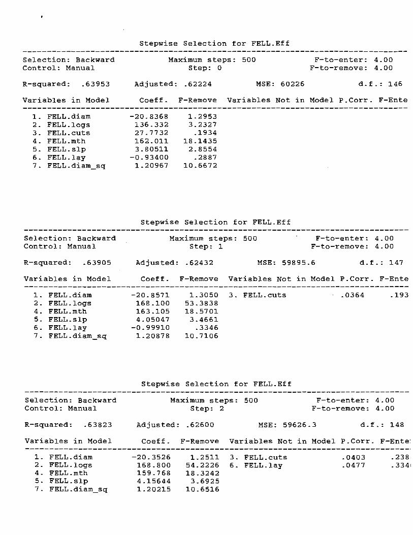
FELL..diamFELL.logsFELL.cutFELL.mthFELL.slpFELL..layFELL.diam_sq

FELLdiamFELL..logs

4. FELL.mth5.. FELL1..slp

FELL..layFELiL..diam_sq

FELL.diamFELL.logsFELL.mthFELL.slp

7. FELL..diam_sq

Stepwise Selection for FELL.Eff

-20.8368136.33227.7732162.0113.80511-0.934001.20967

Stepwise Selection for FELL.Eff

-20.8571168.100163.1054.05047

-0.999101.20878

-20. 3526168.800159.7684... 15644

1.20215

1.29533.2327.1934

18 14352.8554.2887

10.6672

1.3050 3. FELL.cuts53.383818.57013.4661.3346

10.7106

Stepwise Selection for FELL.Eff

1.2511 3. FELL.cuts54.2226 6. FELL.lay18.32423.6925

10.6516

Selection: Backward Maximum steps: 500 F-to-enter: 4.00Control: Manual Step: 0 F-to--remove: 4.00

R-squared: .63953 Adjusted: .62224 MSE: 60226 d.f: 146

Variables in Model Coeff. F-Remove Variables Not in Model P.Corr.. F-Ente

Selection: Backward Maximum steps: 500 F-to-enter: 4.00Control: Manual Step: 1 F-to-remove: 4.00

R-squared: .63905 Adjusted: .62432 MSE: 59895.6 d.f.,: 147

Variables in Model Coeff.. F-Remove Variables Not in Model P..Corr. F-Ente

Selection: Backward Maximum steps: 500 F-to-enter: 4.00Control: Manual Step: 2 F-to-remove: 4.00

R-squared: .63823 Adjusted: .62600 MSE: 59626.3 d.f.: 148

Variables in Model Coeff. F-Remove Variables Not in Model P..Corr. F-Ente:

.0403 - 238

.0477 334

.0364 - 193

Selection: BackwardControl: Manual

R-squared: .63517

Variables in Model

2. FELL.logsFELL.inthFELL..slp

7. FELL..diam_sq

CONSTANTFELL. logsFELL. mthFELL. slpFELL - diamsq

Stepwise Selection for FELL.Eff

Maximum steps: 500Step: 3

Adjusted: .62537

165.820 52.9522 1. FELL.djam151.959 17.1488 3. FELL.cuts4.66382 4.8547 6. FELL.lay0.79873 113.8609

Model fitting results for: FELL..Eff

-240.054485165.819949151.9594414.6638190.798731

108.67400922.78740636.6952932.1167080.074854

F-to-enter: 4.00F-to-remove: 4.00

MSE: 59726.8 d.f.,: 149

t-value

-2.20897.27684.14112. 2033

10.6706

Coeff. F-Remove Variables Not in Model P..Corr.. F-Ente

sig. leve

0.0280. 0001

0. 000:

0. 029:

0. 000

R-SQ. (ADJ.) = 0.6254 SE= 244.390643 MAE= 148.073289 lDurbWat= 2.396Previously: 0.6332 235.682818 168.832022 1.840154 observations fitted, forecast(s) computed for 0 missing val. of dep.. var.

.0916 1.. 251

.0399 .236

.0430 .274

Independent variable coefficient std. error

Stepwise Selection for YARD..PROD

Model fitting results for: YARD.PROD

Independent variable coefficient std. error t-value sigleve

CONSTANT 168.636347 28.684236 5.8791 0.000YARD. YDIS 0.194592 0.030161 6.4517 0.000YARD - LDIS 1.577744 0.183015 8.6209 0 * 000YARD . SET 50.986348 23.156433. 2.2018 0.028YARD - TURN 25.409688 5.356251 4-7439 0.000

R-SQ. (ADJ.,) = 0.4269 SE= 75.462009 MAE= 55.330539 DurbWat= 1.815Previously: 0.0000 0.000000 0.000000 0.000258 observations fitted, forecast(s) computed for 0 missing val.. of dep. var.

Variables in Model Coeff. F-Remove Variables Not in Model P..Corr. F-Ente

1. YARD.YDIS 0.19459 41.. 62412. YARD.L1DIS 1 57774 74. 31933. YARD.SET 50.9863 484804. YARD.TURN 25.. 4097 22. 5049

Selection: Backward Maxinuim steps: 500 F-to-enter: 4.00Control: Manual Step: 0 F-to-remove: 4.00

R-squared: .43587 Adjusted: .42695 MSE: 5694.51 d.f.: 253

APPENDIX E: OWNING ND OPERATING COST CALCULATIONS

The following pages are outputs from the PACE program, a

spreadsheet-driven software package which calculates operating

and ownership costs based on user-input values.

111

Summary

IMMMMMMMMMMMMMMM?MMMMJMJMM?J5 Labor Costs FM1MMMMMMMMMMMMMMMMMMMMMM1qM4'JPJJJS.J

GDDDDDDDDDDDDDDDDDDDDDDDDDDDDDDDDDDDDDDDDDDDDDDDDDDDDDDDDDDDDDDDDDDDDDDDDDDDDDD

: Total number ot workers: # 2.00Total crew wage (Per hour):

$ 37.12: Direct labor cost:

$ 51.97: Supervision and overhead: $ 7.80

Labor cost (Subtotal):$ 59.76

: Total operating cost (Operating+Labor): $ 59.76

Current value = 20.42[ESCJ=Menu (Highlight value to change and press return)

:->Base wage for 1st crew position (Per hour) $ 2042Base wage tor 2nd crew position (Per hour) $ 16.70

: Base wage for 3rd crew position (Per hour) $ 0.00: Base wage tor 4th crew position (Per hour) $ 0.00: Base wage tor 5th crew position (Per hour) $ 0.00

Base wage tor 6th crew position (Per hour) $ 0.00: Fringe benefits 40.00

Travel time per day (Hours) 0.00: Operating time per day (Hours) # 6.00: Percent of direct labor cost for supervision 6 15.00

$ 0.00$ 0.00 I Year$ 0.00 / Year$ 0.00 I Year$ 0.00 / Year$ 0.00 I Hour

$ 0.00 I Hour$ 0.00 / Hour$ 0.00 / Hour$ 0.00 I Hour$ 0.00 I Hour

$ 51.97 I Hour$ 7.80 I Hour$ 59.76 I Hour

$ 0.00 I Hour$ 0.00 I Hour$ 59.76 I Hour$ 59.76 / Hour

*** Felling Crew Labor ***Ownership

Depreciable value:Equipment depreciation:Interest expense:Taxes. license, insurance and storage:Annual ownership cost:Ownership cost (Subtotal):

Machine operatingRepairs and maintenance:Fuel and oil:Lines and rigging:Tires or tracks:Equipment operating cost (Subtota]j:

LaborDirect labor cost:Supervision and overhead:Labor cost (Subtotal):

OWNERSHIP COSTOPERATING COSTLABOR COSTMachine rate (Ownership + Operating + Labor)

*** Press [RETURN1 tor the menu

Summary*** Four Stihi 064 Falling Saws Owning and Operating costs **

OwnershipDepreciable value:Equipment depreciation:Interest expense:Taxes, license, insurance and storage:Annual ownership cost:Ownership cost (Subtotal):

Machine operatingRepairs and maintenance:Fuel and oil:Lines and rigging:Tires or tracks:Equipment operating cost (Subtotal):

LaborDirect labor cost:Supervision and overhead:Labor cost (Subtotal):

OWNERSHIP COSTOPERATING COSTLABOR COSTMachine rate (Ownership + Operating + Labor)

Press [RETURNJ tor the menu ***

$ 1,937.00$ 1,291.33 / Year$ 348.62 I Year$ 54.62 / Year$ 1.694.57 I Year$ 1.09 I Hour

$ 0.75 / Hour$ 0.85 I Hour$ 0..75 I Hour$ 0.50 I Hour$ 2.85 I Hour

$ 000 I Hour$ 0.00 I Hour$ 0.00 / Hour

$ 1..09 / Hour$ 2.85 / Hour$ 0.00 I Hour$ 3.93 I Hour

IMMMMMMMMMMMMMMMMMMMMM1IMM5 Equipment Owner ship CoStS FMMMMMMMMMMMMMMMMMMMMMfrfMMI

GDDDDDDDDDDDDDDDDDDDDDDDDDDDDDDDDDDDDDDDDDDDDDDDDDDDDDDDDDDDDDDDDDDDD1JDDDDDDDD1

HMMMMMMMMMMMMMMMMMMMMMMMMMMMMMMMMMMMMMMMMMMMMMMMMMMMMMMMMMMMMMMIVIMMMMMMMMMMfrIMMMI

Current value = 3,228.00[ESCJ=Menu (Highlight value to change and press return)

IMMMMMMMMMMMMMMMMMMMMMMfrJM5 Equipment Operating Costs FMMMMMMMMMMMMMMMMMMfr1MMMMMJ1

GDDDDDDDDDDDDDDDDDDDDDDDDDDDDDDDDDDDDDDDDDDDDDDDDDDDDDDDDDDDDDDDDDDDDDDDDDDDDDD

Current value = 90.00[ESC}=Menu (Highlight value to change and press return)

:->Delivered equipment cost $ 3,228.00Minus line and rigging cost $ 0.00Minus tire or track replacement cost $ 000Minus residual (salvage) value $ 1,291.00

: Life of equipment (Years) 1.50: Number of days worked per year * 260.00

Number of hours worked per day 6.00: Interest Expense 12.00

Percent of average annual investment for:: Taxes, License, Insurance, and Storage 188

:->Percent of equipment depreciation for repairs 90.00: Fuel amount (Gallons per hour) # 0.23

Fuel cost (Per gallon) $ 1.46: Percent of fuel consumption for lubricants 45.00

Cost of oil and lubricants (Per gallon) $ 5.00: Cost of lines $ 100.00: Estimated life of lines (Hours) * 400.00

Cost of rigging $ 40. 00: Estimated life of rigging (Hours) * 80.00: Cost of tires or tracks $ 619. 00

Estimated life of tires or tracks (Hours) * 1,238.00

: Depreciable value: $ 1,937.00Equipment depreciation: $ 1,291.33

: Average annual investment: $ 2,905.17: Interest expense $ 348.62: Taxes, license, insurance and storage: $ 54.62: Annual ownership cost: $ 1694..57: Annual utilization (Hours per year) # 1,560.00: Ownership cost (Dollars per hour) $ 1.09

: Repairs and maintenance: $ 075Fuel: $ 0.34

: Oil and lubricants: $ 052: Lines: $ 0.25: Rigging: $ 0.50: Tires or tracks: $ 0.50: Equipment operating cost (Subtotal): $ 2.85

Summary*** 1/2-ton 4WD Pickup

*** Press [RETURN1 for the menu

OwnershipDepreciable value: $ 16,668 .00Equipment depreciation: $ 2,083.50 / YearInterest expense: $ 1,347.33 / YearTaxes, license, insurance and storage: $ 211.08 / YearAnnual ownership cost: $ 3..641.91 / YearOwnership cost (Subtotal): $ 1.75 / Hour

Machine operatingRepairs and maintenance: $ 0.50 / HourFuel and oil: $ 1.14 / HourLines and rigging: $ 0.00 / HourTires or tracks: $ 0.20 / HourEquipment operating cost (Subtotal): $ 184 / Hour

LaborDirect labor cost: $ 0.00 / HourSupervision and overhead: $ 0.00 / HourLabor cost (Subtotal): $ 0.00 / Hour

OWNERSHIP COST $ 1.75 / HourOPERATING COST $ 1.84 / HourLABOR COST $ 0.00 / HourMacthine rate (Ownership + Operating + Labor) $ 3.59 / Hour

Current value = 18,520.00[ESCJ=Menu (Highlight value to change and press return)

IMMMMMMMMMMMMMMMMMMMMMMMM5 Equipment Operating Costs FMMMMMfrIMMMMMfrIMMMMMMMMIjMMMM,

:->Percent of equipment depreciation for repairs 50..00: Fuel amount (Gallons per hour) # 0.83

Fuel cost (Per gallon) $ 1.28: Percent of fuel consumption for lubricants 175: Cost of oil and lubricants (Per gallon) $ 5.00: Cost of lines $ 0.00

Estimated life of lines (Hours) * 0.00: Cost of rigging $ 0.00: Estimated life of rigging (Hours) # 0.00: Cost of tires or tracks $ 480.00: Estimated life of tires or tracks (Hours) 2,400.00GDDDDDDDDDDDDDDDDDDDDDDDDDDDDDDDDDDDDDDDDDDDDDDDDDDDDDDDDDDDDDDDDDDDDDDDDDDDDDD

Repairs and maintenance: $ 0.50: Fuel: $ 1.06

Oil and lubricants: $ 0.07: Lines: $ 0.00: Rigging: $ 0.00

Tires or tracks: $ 0.20: Equipment operating cost (Subtotal) $ 1.84

HMMMMMMMMMMMMMMMMMMMMMMMMMM1MMIIJMMMMMMIMMMMIMMMMMJMMMMMMMMMJMMJMCurrent value = 50.00

[ESCJ=Menu (Highlight value to change and press return)

IMMMMMMMMMMMMMMMMMJfMJfMM5 Equipment Ownership Costs

:->IDelivered equipment cost

FMMMMMMMMMMMMMIMMIII

$ 18,520.00Minus line and rigging cost $ 0.00Minus tire or track replacement cost $ 0.00Minus residual (salvage) value $ 1,852.00

: Life of equipment (Years) 8.00: Number of days worked per year # 260.00

Number of hours worked per day # 8.00: Interest Expense 12.00: Percent of average annual investment for:: Taxes, License, Insurance, and Storage 1.88

: Depreciable value: $ 16,668.00: Equipment depreciation: $ 2,083.50

Average annual investment: $ 11,227.75: Interest expense: $ 1,347.33: Taxes, license, insurance and storage: $ 211.08: Annual ownership cost: $ 3,641.91: Annual utilization (Hours per year) : * 2:080.00: Ownership cost (Dollars per hour): $ 1.75

)

SummaryYarding Crew Labor Only

OwnershipDepreciable value:Equipment depreciation:Interest expense:Taxes, license, insurance and storage:Annual ownership cost:Ownership cost (Subtotal):

Machine operatingRepairs and maintenance:Fuel and oil:Lines and rigging:Tires or tracks:Equipment operating cost (Subtotal):

LaborDirect labor cost:Supervision and overhead:Labor cost (Subtotal):

OWNERSHIP COSTOPERATING COSTLABOR COSTMachine rate (Ownership + Operating + Labor)

*** Press [RETURN] for the menu **

GDDDDDDDDDDDDDDDDDDDDDDDDDDDDDDDDDDDDDDDDDDDDDDDDDDDDDDDDDDDDDDDDDDDDDDDDDDDDDD

: Total number of workers: 6.00: Total crew wage (Per hour): $ 66.76: Direct labor cost: $ 93.46: Supervision and overhead: $ 14.02: Labor cost (Subtotal): $ 107.48: Total operating cost (Operating+Labor): $ 107..48

Current value = 11..93[ESC}=Menu (Highlight value to change and press return)

$ 0.00$ 0.00 / Year$ 0.00 / Year$ 0.00 / Year$ 0.00 / Year$ 0.00 / Hour

$ 0.00 / Hour$ 0.00 / Hour$ 0.00 / Hour$ 0.00 / Hour$ 0.00 / Hour

$ 93.46 / Hour$ 14..02 / Hour$ 107.48 / Hour

$ 0.00 / Hour$ 0.00 / Hour$ 107.48 / Hour$ 107.48 / Hour

IMMMMMMMfrIMMMMMMMMMMMMMMMM?qMMMMM5 Labor Costs FMMMIVIMMMMM MMMMMMMMMMM

:->Base wage for 1st crew position (Per hour) $ 11.. 93: Base wage for 2nd crew position (Per hour) $ 10.34: Base wage for 3rd crew position (Per hour) $ 10.34

Base wage for 4th crew position (Per hour) $ 12.. 45Base wage for 5th crew position (Per hour) $ 10. 85Base wage for 6th crew position (Per hour) $ 10.85

: Fringe benefits 40. 00Travel time per day (Hours) 0.00Operating time per day (Hours) 8 00Percent of direct labor cost for supervision 15. 00

e

SummaryTTY5O Yarder/Danebo MSP Carriage Owning and Operating Costs ***

OwnershipDepreciable value:Equipment depreciation:Interest expense:Taxes, license, insurance and storage:Annual ownership cost:Ownership cost (Subtotal):

Machine operatingRepairs and maintenance:Fuel and oil:Lines and rigging:Tires or tracks:Equipment operating cost (Subtotal):

LaborDirect labor cost:Supervision and overhead:Labor cost (Subtotal):

OWNERSHIP COSTOPERATING COSTLABOR COSTMachine rate (Ownership + Operating + Labor)

*** Press [RETURN] for the menu

$ 323,790.00$ 40,473.75 / Year$ 37,095.68 / Year$ 7,202.74 / Year$ 84,772.16 / Year$ 40.76 / Hour

$ 9.73 / Hour$ 12.06 / Hour$ 1719 / Hour$ 1.25 / Hour$ 40.23 / Hour

$ 0.00 / Hour$ 0.00 / Hour$ 0.00 / Hour

$ 40.76 / Hour$ 40.23 / Hour$ 0.00 / Hour$ 80.98 / Hour

*

IMMMMMMfrfMMMM4MMjffjq5 Equipment Ownership Costs FMMMMMMMMfrfMMfJfjj:->Delivered equipment cost

$ 475,000.00Minus line and rigging cost $ 47,340.00Minus tire or track replacement cost $ 8,000 00Minus residual (salvage) value $ 95,870.00

: Life of equipment (Years) 8.00: Number of days worked per year 260.00: Number of hours worked per day # 8..00

Interest Expense 12..00: Percent of average annual investment for:: Taxes, License, Insurance, and Storage 2.33GDDDDDDDDDDDDDDDDDDDDDDDDDDDDDDDDDDDDDDDDDDDDDDDDDDDDDDDDDDDDDDDDDDDDDDDD

Depreciable value:$ 323,790..00

Equipment depreciation:$ 40,473.75

: Average annual investment:$ 309,130.62

: Interest expense:$ 37,095.68

: Taxes, license, insurance and storage: $ 7,202.74: Annual ownership cost:

$ 84772.16: Annual utilization (Hours per year): 2,080.00: Ownership cost (Dollars per hour): $ 40.76

Current value = 475,000..00[ESCJ=Menu (Highlight value to change and press return)

I1MMMMMfrIMMMM)flflvffrIfjfMMfrffrfM5 Equipment Operating Costs FMMMMMMMMMMMMMMfMMMM1M

Current value = 50..00[ESCJ=Menu (Highlight value to change and press return)

:->Percent of eauipment depreciation for repairs 5000: Fuel amount (Gallons per hour) # 13.00: Fuel cost (Per gallon)

$ 0.84Percent of fuel consumption for lubricants 1.75Cost of oil and lubricants (Per gallon) $ 5.00

: Cost of lines$ 31,299..00

: Estimated life of lines (Hours) * 2,375.00: Cost of rigging

$ 16,041..00Estimated life of rigging (Hours) * 4,000.00Cost of tires or tracks

$ 8,000.00: Estimated life of tires or tracks (Hours) * 6,400..00GDDDDDDDDDDDDDDDDDDDDDDDDDDDDDDDDDDDDDDDDDDDDDDDDDDDDDDD: Repairs and maintenance:

$ 9.73Fuel:$ 10.92

: Oil and lubricants:$ 1.14Lines:$ 13.18

: Rigging:$ 401

: Tires or tracks:$ 1.25

: Equipment operating cost (Subtotal): $ 40.23

SummaryYarding Crew Crummies 1/2-ton 4WD PU + 4WD Suburban

OwnershipDepreciable value:Equipment depreciation:Interest expense:Taxes, license, insurance and storage:Annual ownership cost:Ownership cost (Subtotal):

Machine operatingRepairs and maintenance:Fuel and oil:Lines and rigging:Tires or tracks:Equipment operating cost (Subtotal):

LaborDirect labor cost:Supervision and overhead:Labor cost (Subtotal):

OWNERSHIP COSTOPERATING COSTLABOR COSTMachine rate (Ownership + Operating + Labor)

*** Press [RETURN] for the menu

$ 36,108.00$ 4,513.50 / Year$ 3,020.58 / Year$ 586.50 / Year$ 8,120.58 / Year$ 3.90 / Hour

$ 1.08 / Hour$ 227 / Hour$ 0.00 / Hour$ 0.52 / Hour$ 3.88 / Hour

$ 0.00 / Hour$ 0.00 / Hour$ 0.00 / Hour

$ 3.90 / Hour$ 3.88 / Hour$ 0.00 / Hour$ 7.78 / Hour

IMMMMMMMMMMMMMMMMMMMMMMMM5 Equ ipine n t Ownership Costs FMMMMMMMMMMMMMMMMMMMMMJMM

:->Delivered equipment cost $ 41,520.00Minus line and rigging cost $ 0.00Minus tire or track replacement cost $ 1.260..00Minus residual (salvage) value $ 4,152..00

Life of equipment (Years) # 8.00: Number of days worked per year # 260.00

Number of hours worked per day # 8.00: Interest Expense 12..00: Percent of average annual investment for:: Taxes, License, Insurance, and Storage 2.33GDDDDDDDDDDDDDDDDDDDDDDDDDDDDDDDDDDDDDDDDDDDDDDDDDDDDDDDDDDDDDDDDDDDDDDDDDDDDDD

Depreciable value: $ 36,108..00: Equipment depreciation: $ 4513-50: Average annual investment: $ 25,171.50

Interest expense: $ 3,020.58Taxes, licenser insurance and storage: $ 586.50

: Annual ownership cost: $ 8,120.58Annual utilization (Hours per year): # 2,080.00Ownership cost (Dollars per hour): $ 3.90

Current value = 41 .520.00[ESCJ=Menu (Highlight value to change and press return)

1MM! MM MMMMMMMMMMMMMMMM5 Equipment Operating Costs FMMMIVIMMMMMMZPIMMMMMMMMMMMMMM

GDDDDDDDDDDDDDDDDDDDDDDDDDDDDDDDDDDDDDDDDDDDDDDDDDDDDDDDDDDDDDDDDDDDDDDDDDDDDDD: Repairs and maintenance: $ 1.08: Fuel: $ 2.12: Oil and lubricants: $ 0.15

Lines: $ 0.00Rigging: $ 0.00Tires or tracks: $ 0.52

: Equipment operating cost (Subtotal): $ 3.88

Current value = 50.00[ESC]=Menu (Highlight value to change and press return)

:->Percent of equipment depreciation for repairs 50.00Fuel amount (Gallons per hour) 1..66

: Fuel cost (Per gallon) $ 1.28: Percent of fuel consumption for lubricants 1.75: Cost of oil and lubricants (Per gallon) $ 5.00

Cost of lines $ 0.00: Estimated life of lines (Hours) # 0.00: Cost of rigging $ 0.00: Estimated life of rigging (Hours) # 0.00: Cost of tires or tracks $ 1,260.00: Estimated life of tires or tracks (Hours) 2,400.00

Summary*** John Deere 648 Grapple Skidder

OwnershipDepreciable value:Equipment depreciation:Interest expense:Taxes, license, insurance and storage:Annual ownership cost:Ownership cost (Subtotal):

Machine operatingRepairs and maintenance:Fuel and oil:Lines and rigging:Tires or tracks:Equipment operating cost (Subtotal):

LaborDirect labor cost:Supervision and overhead:Labor cost (Subtotal):

OWNERSHIP COSTOPERATING COSTLABOR COSTMachine rate (Ownership + Operating + Labor)

*** Press [RETURN1 for the menu

$ 97,316.00$ 32,438.67 I Year$ 11,528.00 I Year$ 2,23835 I Year$ 46,205.02 I Year$ 22.21 I Hour

$ 9.36 / Hour$ 1.03 / Hour$ 0.00 / Hour$ 1.87 / Hour$ 12.26 I Hour

$ 0.00 / Hour$ 0.00 / Hour$ 0.00 / Hour

$ 22.21 I Hour$ 12.26 I Hour$ 0.00 / Hour$ 34.47 I Hour

IMMMMMMMfrfMfrfMMMgffrfMjjJj5 Equipment Ownership Costs FMMMMMMMMMMMMMMMMMMMMiI1

:->Delivered equipment cost $ 131,000.00Minus line and rigging cost $ 0.00Minus tire or track replacement cost $ 7,484.00Minus residual (salvage) value $ 26,200..00

: Life of equipment (Years) 3.00Number of days worked per year 260.00

: Number of hours worked per day 8.00Interest Expense 12.00

: Percent of average annual investment for:: Taxes, License, Insurance, and Storage 2.33GDDDDDDDDDDDDDDDDDDDDDDDDDDDDDDDDDDDDDDDDDDDDDDDDDDDDDDDDDDDDDDDDDDDDDDDDDDDDDD: Depreciable value: $ 97,316.00

Equipment depreciation: $ 327438.67: Average annual investment: $ 96,066.66: Interest expense: $ ll,528..00: Taxes, license, insurance and storage: $ 2,238.35

Annual ownership cost: $ 46,205.02: Annual utilization (Hours per year): # 2..080..00

Ownership cost (Dollars per hour): $ 22.21

Current value = 131,000.00[ESCJ=Menu (Highlight value to change and press return)

IMMMMMMMMMMMMMMMMMfrJMMMMMJvI5 Equipment Operating Costs FMMMMMMMMMMMMMMMMMMMMMMMMM

:->Percent of equipment depreciation for repairs 60..00: Fuel amount (Gallons per hour) 1_li

Fuel cost (Per gallon) $ 0.84: Percent of fuel consumption for lubricants 1.75

Cost of oil and lubricants (Per gallon) $ 5.00Cost of lines $ 0.00

: Estimated life of lines (Hours) # 0.00: Cost of rigging $ 0.00: Estimated life of rigging (Hours) 0.00

Cost of tires or tracks $ 7,484.00Estimated life of tires or tracks (Hours) 4,000.00

GDDDDDDDDDDDDDDDDDDDDDDDDDDDDDDDDDDDDDDDDDDDDDDDDDDDDDDDDDDDDDDDDDDDDDDDDDDDI,DD: Repairs and maintenance: $ 9.36: Fuel: $ 0..93

Oil and lubricants: $ 0_la: Lines: $ 0.00: Rigging: $ 0.00: Tires or tracks: $ 1.87: Equipment operating cost (Subtotal): $ 12.26

Current value = 60.00[ESC]=Menu (Highlight value to change and press return)

SummaryTailhold Crawler Tractor

OwnershipDepreciable value:Equipment depreciation:Interest expense:Taxes, license, insurance and storage:Annual ownership cost:Ownership cost (Subtotal):

Machine operatingRepairs and maintenance:Fuel and oil:Lines and rigging:Tires or tracks:Equipment operating cost (Subtotal):

LaborDirect labor cost:Supervision and overhead:Labor cost (Subtotal):

OWNERSHIP COSTOPERATING COSTLABOR COSTMachine rate (Ownership + Operating + Labor)

*** Press [RETURN] for the menu ***

$ 60,000.00$ 15.000.00 / Year$ 6,300.00 / Year$ 1,223.25 / Year$ 22 .523.25 / Year$ 10.83 / Hour

$ 2.88 / Hour$ 0.49 / Hour$ 0.00 / Hour$ 0.00 / Hour$ 3.38 I Hour

$ 0.00 / Hour$ 0.00 / Hour$ 0.00 / Hour

$ 10.83 / Hour$ 338 / Hour$ 0.00 / Hour$ 14.20 / Hour

IMMMMMMMMMMMMMMMjffvj7vffvj7vf5 Equipment Ownership Costs FMMMMMMMMMMMMMMMMMM!1fl1

:-)Delivered equipment cost $ 75,000.00Minus line and rigging cost $ 0.00Minus tire or track replacement cost $ 0..00Minus residual (salvage) value $ 15,00000

: Life of equipment (Years) 4.00: Number of days worked per year # 260.00

Number of hours worked per day 8.00: Interest Expense 12.00

Percent of average annual investment for:: Taxes, License, Insurance, and Storage 2.33GDDDDDDDDDDDDDDDDDDDDDDDDDDDDDDDDDDDDDDDDDDDDDDDDDDDDDDDDDDDDDDDDDDDDDDDDDDDDDD: Depreciable value: $ 60,000.00: Equipment depreciation: $ 15:00000: Average annual investment: $ 52,500.00

Interest expense: $ 6.300.00: Taxes, license, insurance and storage: $ 1,223.25

Annual ownership cost: $ 22,523.25: Annual utilization (Hours per year): * 2,080.00: Ownership cost (Dollars per hour): $ 10.83

Current value = 75,000.00[ESCJ=Menu (Highlight value to change and press return)

IMMMMMMMMMMMMMMMMMMMfrJfrJfrJMM5 Equipment Operating Costs FMMMMMMMMMMMMMMMMMMMMMMMMM

GDDDDDDDDDDDDDDDDDDDDDDDDDDDDDDDDDDDDDDDDDDDDDDDDDDDDDDDDDDDDDDDDDDDDDDDDDDDDDD

Current value = 40.00[ESC]=Menu (Highlight value to change and press return)

:-Percent of equipment depreciation for repairs 40..00: Fuel amount (Gallons per hour) 0.53: Fuel cost (Per gallon) $ 0.84: Percent of fuel consumption for lubricants 175: Cost of oil and lubricants (Per gallon) $ 5.00

Cost of lines $ 0.00Estimated life of lines (Hours) 0.00Cost of rigging $ 0..00Estimated life of rigging (Hours) 0..00Cost of tires or tracks $ 0.00

: Estimated life of tires or tracks (Hours) 0.00

: Repairs and maintenance: $ 2.88Fuel: $ 0..45Oil and lubricants: $ 0..05

: Lines: $ 0.00Rigging: $ 0.00

: Tires or tracks: $ 0.00Equipment operating cost (Subtotal): $ 3.38

OWNERSHIP COSTOPERATING COSTLABOR COSTMachine rate (Ownership + Operating + Labor)

*** Press [RETURNJ tor the menu ***

Sumrrary*** Fire Truck Owning and Operating Costs *

OwnershipDepreciable value:Equipment depreciation:Interest expense:Taxes, license, insurance and storage:Annual ownership cost:OwnershIp cost (Subtotal):

Machine operatingRepairs and maintenance:Fuel and oil:Lines and rigging:Tires or tracks:Equipment operating cost (Subtotal):

LaborDirect labor cost:Supervision and overhead:Labor cost (Subtotal):

$ 9 , 000 . 00

$ 1,125.00 I Year$ 727.50 / Year$ 141.26 I Year$ 1,993.76 I Year$ 0.96 / Hour

$ 0.16 I Hour$ 0.00 I Hour$ 0.00 I Hour$ 0.00 / Hour$ 0.16 I Hour

$ 0.00 / Hour$ 0.00 I Hour$ 0.00 I Hour

$ 0.96 I Hour$ 0.16 I Hour$ 0..00 I Hour$ 1.12 I Hour

IM1MMMMMMMMMMMMMMMMMMMMM5 Equipment Ownership Costs FMMMMMMMMMMMMMMM1MMM?V2PIM

:->Delivered equipment cost$ 10,000.00

Minus line and rigging cost $ 0.00Minus tire or track replacement cost $ 0.00Minus residual (salvage) value $ 1,000.00

Life of equipment (Years) 8.00: Number of days worked per year # 260.00: Number of hours worked per day 8.00

Interest Expense 12.00Percent of average annual investment for:

: Taxes, License, Insurance, and Storage 2.33GDDDDDDDDDDDDDDDDDDDDDDDDDDDDDDDDDDDDDDDDDDDDDDDDDDDDDDDDDDDDDDDDDDDDDDDDDD: Depreciable value:

$ 9,000.00Equipment depreciation:

$ 1125.00: Average annual investment:

$ 6.062.50: Interest expense:

$ 727.50: Taxes, license, insurance and storage: $ 141.26: Annual ownership cost: $ 1,993.76

Annual utilization (Hours per year): 2:080.00Ownership cost (Dollars per hour): $ 0.96

HMMMMMMMMMMMMMMMMMMMMMMMMMMMMMMMMMIMMMMMMfrIMIIIIJJICurrent value = 10000.00

[ESC]=Menu (Highlight value to change and press return)

IMMMKMMMMMMMMMfMJçjjf5 Equipment Opera t ± ng Costs FMMMMMMMMMMMrMMMMMMM?V2PIMJ

HMMMMMMMMMMMMMMMMMMMMMMMMMMMMMMMMMMMMMMMMMMM?MMMMM?MMMMMMM?MMCurrent value = 30.00

[ESC]=Menu (Highlight value to change and press return)

:->Percent ot equipment depreciation tor repairs 30.00: Fuel amount (Gallons per hour) # 0.00

Fuel cost (Per gallon) $ 0.00Percent ot tuel consumption for lubricants 0.00Cost of oil and lubricants (Per gallon) $ 0.00

: Cost ot lines$ 0..00

: Estimated lite ot lines (Hours) # 0.00: Cost ot rigging

$ 0.00: Estimated lite of rigging (Hours) # 0.00: Cost of tires or tracks

$ 0..00Estimated life ot tires or tracks (Hours) # 0.00

GDDDDDDDDDDDDDDDDDDDDDDDDDDDDDDDDDDDDDDDDDDDDDDDDDDDDDDDRepairs and maintenance:

$ 0.16: Fuel:

Oil $ 0.00: and lubricants:

Lines: $ 0.00$ 0.00

: Rigging:$ 0.00

: Tires or tracks:$ 0.00

: Equipment operating cost (Subtotal): $ 0..16

Summary*** Ownership and Labor for Tail/tnt Support/Anchor Rigging and Tools ***

OwnershipDepreciable value:Equipment depreciation:Interest expense:Taxes, license, insurance and storage:Annual ownership cost:Ownership cost (Subtotal):

Machine operatingRepairs and naintenance:Fuel and oil:Lines and rigging:Tires or tracks:Equipment operating cost (Subtotal):

LaborDirect labor cost:Supervision and overhead:Labor cost (Subtotal):

OWNERSHIP COSTOPERATING COSTLABOR COSTMachine rate (Ownership + Operating + Labor)

*** Press [RETURN] for the menu

$ 35,673.00$ 14,269.20 / Year$ 2,996.53 / Year$ 581.83 / Year$ 17,847..56 / Year$ 8.58 / Hour

$ 0.00 / Hour$ 0..00 / Hour$ 0.00 / Hour$ 0..00 / Hour$ 0.00 / Hour

$ 17.84 / Hour$ 2.68 / Hour$ 20.51 / Hour

$ 8.58 / Hour$ 0.00 / Hour$ 20.51 / Hour$ 29.09 / Hour

IMMMMMMMMMMMMMMMMMMMMJMM5 Equipment Ownership Costs FMMMMMMMMMMMMMMMMMMMMMMMM1

:->Delivered equipment cost $ 35.673.00Minus line and rigging cost $ 0.00Minus tire or track replacement cost $ 0.00Minus residual (salvage) value $ 0.00

: Life of equipment (Years) # 2..50Number of days worked per year # 260.00Number of hours worked per day 8.00Interest Expense 12.00

: Percent of average annual investment for:: Taxes, License, Insurance, and Storage 233GDDDDDDDDDDDDDDDDDDDDDDDDDDDDDDDDDDDDDDDDDDDDDDDDDDDDDDDDDDDDDDDDDDDDDDDDDDDDDD: Depreciable value: $ 35,673..00: Equipment depreciation: $ 14,269.20: Average annual investment: $ 24,971.10: Interest expense: $ 2,996..53

Taxes, license, insurance and storage: $ 581.83: Annual ownership cost: $ 17,847.56

Annual utilization (Hours per year): 2,080.00Ownership cost (Dollars per hour): $ 8.58

Current value = 35,673.00[ESCJ=Menu (Highlight value to change and press return)

IMMMMMMMMMMMMMMMMMMMMMMMMMMMMMM5 Labor Costs FMMMMMMMMMMMMZqMMMMMMMMMMMMMMMMMMMM

GDDDDDDDDDDDDDDDDDDDDDDDDDDDDDDDDDDDDDDDDDDDDDDDDDDDDDDDDDDDDDDDDDDDDDDDDDDDDDD

: Total number of workers: * 1.00: Total crew wage (Per hour): $ 12..74: Direct labor cost: $ 17.84

Supervision and overhead: $ 2.68Labor cost (Subtotal): $ 20.51

: Total operating cost (Operating+Labor): $ 20.51

Current value = 12.74[ESCJ=Menu (Highlight value to change and press return)

:->Base wage for 1st crew position (Per hour) $ 12.74Base wage for 2nd crew position (Per hour) $ 0.00

: Base wage for 3rd crew position (Per hour) $ 0.00: Base wage for 4th crew position (Per hour) $ 0..00: Base wage for 5th crew position (Per hour) $ 0.00: Base wage for 6th crew position (Per hour) $ 0.00

Fringe benefits 40.00Travel time per day (Hours) # 0.00Operating time per day (Hours) # 8.00Percent of direct labor cost for supervision 15.00

Summary*** John Deere Log Loader

OwnershipDepreciable value:Equipment depreciation:Interest expense:Taxes, license, insurance and storage:Annual ownership cost:Ownership cost (Subtotal):

Machine operatingRepairs and maintenance:Fuel and oil:Lines and rigging:Tires or tracks:Equipment operating cost (Subtotal):

LaborDirect labor cost:Supervision and overhead:Labor cost (Subtotal):

OWNERSHIP COSTOPERATING COSTLABOR COSTMachine rate (Ownership + Operating + Labor)

*** Press [RETURN) for the menu ***

Total number of workers:Total crew wage (Per hour)

: Direct labor cost:: Supervision and overhead:: Labor cost (Subtotal):: Total operating cost (Operating+Labor):

Current value = 12.83[ESCJ=Menu (Highlight value to change and press return)

GDDDDDDDDDDDDDDDDDDDDDDDDDDDDDDDDDDDDDDDD.DDDDDDDDDDDDDDDDDDDDDDDDDDDDDDDDDDDDDDI

1 .0012.8317 .962.69

20.6637.91

JD 892D-LC

$ 216 300.00$ 27,037.50 I Year$ 22,542.00 I Year$ 4,376.90 / Year$ 53956.41 / Year$ 23.06 [Hour

$ 7.51 / Hour$ 7.42 I Hour$ 0.00 I Hour$ 2.33 I Hour$ 17.26 I Hour

$ 17.96 / Hour$ 2..69 I Hour$ 20.66 I Hour

$ 23.06 I Hour$ 17.26 / Hour$ 20.66 I Hour$ 60.97 I Hour

IMMMMMMMMMMMMMMMMMMMMMfrIIfrIMMMMM5 Labor Costs FMMMMMMMMMMM MMMMMMMM

:->Base wage for 1st crew position (Per hour) $ 12.83Base wage for 2nd crew position (Per hour) $ 0.00

: Base wage for 3rd crew position (Per hour) $ 0.00: Base wage for 4th crew position (Per hour) $ 0.00

Base wage for 5th crew position (Per hour) $ 0.00: Base wage for 6th crew position (Per hour) $ 0.00: Fringe benefits 40.00: Travel time per day (Hours) # 0.00: Operating time per day (Hours) # 9.00

Percent of direct labor cost for supervision 15.00

IMMMMMMMMMMMMMMMMMMMMMMMM5 Equipment Ownership Costs FMMMMMMMMMMMMMMMMMMMMMJrfJ

289,000.000.00

14,900.0057,800.00

8.00: Number of days worked per year 260.00: Number of hours worked per day 9.00: Interest Expense 12.00: Percent of average annual investment for:

Taxes, License, Insurance, and Storage 2.33GDDDDDDDDDDDDDDDDDDDDDDDDDDDDDDDDDDDDDDDDDDDDDDDDDDDDDDDDDDDDDDDDDDDDDDDDDDDDDD

Depreciable value: $ 216300.00: Equipment depreciation: $ 27,037.50

Average annual investment: $ 187:850.00: Interest expense: $ 22,542..00: Taxes, license, insurance and storage: $ 4,376.90: Annual ownership cost: $ 53,956.41: Annual utilization (Hours per year): * 2,340.00

Ownership cost (Dollars per hour): $ 23.06

Current value = 289,000.00[ESC]=Menu (Highlight value to change and press return)

IMMMMMMMMMMMMMMMfrfMfjqf5 Equipment Operating Costs FIVIMMMMMMMMMMMMMMMMMMMMMMMM

:->Percent of equipment depreciation for repairs 65.00: Fuel amount (Gallons per hour) # 8.00

Fuel cost (Per gallon) $ 0.84Percent of fuel consumption for lubricants 1.75Cost of oil and lubricants (Per gallon) $ 5.00Cost of lines $ 0.00Estimated life of lines (Hours) # 0.00Cost of rigging $ 0.00

: Estimated life of rigging (Hours) # 0.00Cost of tires or tracks $ 14,900.00

: Estimated life of tires or tracks (Hours) 6,400.00GDDDDDDDDDDDDDDDDDDDDDDDDDDDDDDDDDDDDDDDDDDDDDDDDDDDDDDDDDDDDDDDDDDDDDDDDDDDDDD: Repairs and maintenance: $ 7.51

Fuel: $ 6.72Oil and lubricants: $ 0.70

: Lines: $ 0.00: Rigging: $ 0.00: Tires or tracks: $ 2.33: Equipment operating cost (Subtotal): $ 17.26

Current value = 65.00[ESC]=Menu (Highlight value to change and press return)

:->Delivered equipment cost $Minus line and rigging cost $Minus tire or track replacement cost $Minus residual (salvage) value $

Life of equipment (Years)