stochastic processes and their

Stochastic Processes and their Applications 73 (1998) 4748 applications

Product of two multiple stochastic integrals with respect to a normal martingale

Francesco Russo a, Pierre Vallois b,* a Universitt Paris Nord, Institut Galike, Dtfpartement de Mathtmatiques. Au. J.B. Ckment.

F-93430 Villetaneuse, France b Universitk de Nancy I, DPpartement de Mathbmatiques, BP 239, F 54506 Vandoeuvre-les-Nancy

Cedex, France

Received 15 June 1995; revised 13 February 1997

Abstract

Let M be a normal martingale (i.e. (M,M) (t) = t), we decompose the product of two multiple stochastic integrals (with respect to M) In(f)l,,,(g) as a sum of n A m terms Hk. l& is equal to the integral over rW”, of the function t + I n+,,,__2k(hk(l, .)), with respect to the k-tensor product of d[M,M]., hk being an explicit function depending only on f and g. Our formula generalizes the well-known result concerning Brownian motion and compensated Poisson process and allows us to improve some results of Emery related to the chaos representation property of solution of the structure equation. @ 1998 Elsevier Science B.V. All rights reserved

Keywords: Normal martingale; Chaos representation property AMS class$cation: 60644; 60H05; 60H07; 60565

1. Introduction

( 1) In his historical paper, It6 (195 1) proved that the Brownian motion B has the chaos representation property (CRP). This means that every square integrable random variable Z measurable with respect to the o-algebra generated by the Brownian motion can be written as an infinite sum of n-multiple stochastic integrals. We know that the compensated Poisson process N = (N,(t) - t; t 2 0), where NO is a usual Poisson process, also satisfies the CRF’.

A martingale M is called by Dellacherie et al. (1992) a normal martingale if it is locally square integrable and

(M,M) (t) = t, vt >o. (1.1)

Since (A4,M) is the dual projection of [M,M], Eq. (1.1) is equivalent to: (A4: - t; t 20) is a martingale.

We observe that N and B are two normal martingales. Using the fact that (M,M) is a deterministic process, Meyer (1976) constructed by isometry Z,(f), the n-multiple

* Corresponding author. Fax: 83 28 09 89.

0304-4149/98/$19.00 @ 1998 Elsevier Science B.V. All rights reserved PII so304-4149(97)00101-4

48 F. Russo, P. Valloisl Stochastic Processes and their Applications 73 (1998) 4768

integral off with respect to M, when f is an element of L,2(rW;), the set of symmetric and square integrable functions defined on R;.

If A4 = B, Shigekawa (1980) and Meyer (1986) proved that the product of Z,(f) and G(g) is a finite and explicit sum of k-multiple integrals, k < max(n, m). Kabanov (1975) considered a compensated Poisson measure based on a “good” measure space (T, g’, 2). This author proved a similar result concerning the product: Zn( f &(g). This study was extended by Surgailis (1984) and Tudor (1996) to products of k multiple integrals. The formula is complicated and makes use of diagrams.

(2) In this paper we deal with a normal martingale M, and we consider the product: Z,(f &(g). In Section 3 (Theorem 3.4), we establish:

Mf Mg) = 4z+m(ho) + c lk Z,+,-2k(hk)(t)~rMl(dt), (1.2) l<kQmAn +

where ho = f CQg, hk(u,v,t) = f(u,t)g(u,t); t E R:, u E R”,-k, v E (WTpk, l<k<n

A m, $&(dt) = d[M,M](ti) @ . . . @ d[M,M](t,), t = (tl,. . . , tp), Z:(h)(t), t E Rk, is considered as a suitable version of t --+ I,(h(., t)).

When we replace pFM,(dt) with dt, previous identity coincides with the classical formula of the Brownian case.

In terms of Meyer (1986) terminology, Eq. (1.2) corresponds to

MA MB = MAAB d[M,MlAnB. (1.3)

The difficulty consists in giving a precise meaning of this symbolic identity and espe- cially the intertwinning of Stieltjes and stochastic integrations.

Assume for simplicity that m = 1. Eq. (1.2) can be written in the following form:

Mf K(g) = L+l(ho) + n s ajI,I_,(~~)(t)g(f)d[M,MI(t), 0

(1.4)

where Hi(u, t) = f (u, t); u E We’, t > 0. The proof of Eq. (1.2) requires a precise definition of (Z/(f)(t); t E W$), f being

an element of L2(Ryp) an d we also need an L2 estimate of this process. This is done in Section 2. Then we check Eq. (1.2) in Section 3.

(3) We give a second application of Eq. (1.2). Assume that MO is a constant. One says that M has the predictable representation property (PRP) if every random variable Z in L’(O) is equal to E(Z) + so” H, d&l,, where H is a predictable process such that &Jo” H,’ ds) < 00.

We notice that Mf belongs to L2(s2), therefore the PRP implies

t t kf: =lqkff)+

s H,cWl, =E(@)+t+ H,biM,.

0 s 0

Otherwise, by Ito formula we have

J t

n/r: =A4,2+2 M,- dM, + wdwt. 0

I? Russo, P. ValloislStochastic Processes and their Applications 73 (1998) 47-68 49

Consequently, there is a process @ such that,

s

t

[MM], = t+ @(s)dMs. (1.5) 0

Eq. (1 S) is called a structure equation (Emery, 1989; Dermoune, 1995). Several authors considered this equation, see, for instance, Attal and Emery (1994) Azema and Yor (1989), Dermoune (1995) and Emery, 1989. Consequently, this equation is a necessary condition for M to have the PRP.

We say @ is linear if

Q(s) = a(s) + B(s)K-,

where CI and b are two locally bounded functions defined on [w+.

(1.6)

We recall: (i) U(S) = /I?(s) = 0, h4 is a Brownian motion,

(ii) CL(S) = or,fl(s) = 0, M is a Poisson martingale, (iii) g(s) = 0,/I(s) = -1, M is the Azema martingale.

If x = 0, /3 -_ p E [-2,0], Emery (1989) and Azema showed that M has the CRP, which means that every following development:

where fn E L@F). We observe that the CRP implies the PRP.

and Yor (1989), if /I = -1 r.v. Z in L2(0) admits the

The aim of Section 4 concerns the case that @ is a linear functional, i.e.:

[MN], = t + I

‘(c+) + fl(s)M,-)dK. (1.7) 0

Let us suppose that M satisfies the CRP and Eq. (1.7) holds. Applying Eq. (1.2) with m = 1, we show that any polynomial P(M(tr ), . . . ,M(t,)) admits a finite chaos development. Moreover, if o! = 0 and B(s) E [-2,0], we establish that M verifies the CRP. This extends the results of Emery (1989) and Azema and Yor (1989).

2. Notations and preliminary results

Notations. (1) (a, F = (pf; t 3 O),P), will denote a classical filtered probability space, B satisfying the usual conditions. 9 is the o-algebra generated by the predictable processes. M is a normal martingale (Dellacherie et al., 1992, p. 199), if A4 is a martingale, is a locally square integrable martingale and,

(M,M) (t) = t; vt>o. (2.1)

Recall that (k&M) is the dual projection of [M,M], in particular,

E [/” 0

K,d[M,MlW] =E [i=kdj >

K being a positive and predictable process.

(2.2)

50 F Russo, P. Valloisl Stochastic Processes and their Applications 73 (1998) 4768

(2) Let f : lF!T -+ IL!, and g : R’J --f IF!, we set,

(f @ s)(t1 ,...,Gl,Sl, . . . . &n) =f(tl,...,t,)g(sl,...,s,),

fr running over all permutations of { 1,2,. . , , n}. j is called the symmetrization of f.

llfllf = s,_ f(tl,...,tn)2dt, . ..dtn. +

L~(rW~) is the set of functions f E L2(Ry) such that f is a symmetric function of it variables. By convention Lz(rW”,) = ~2(lR~) = R.

(3) Let us define,

G = {(t1 ,...,tn); 0 < t1 < ... < t,}, D, = {(tl ,...,tn); 3i#j,ti = tj}.

57: will denote the simple functions f of the following type:

f is symmetric and f = llo,,b,l @ . . . 63 ll,n,b~, on C,,, (2.3)

where 0 < al -c 61 < a2 -c b2 -c ... < a,, < b,. If p 2 1, Y4”,p is the set of functions cp : Rnfp + R,

cP=f@s (2.4)

where f E 9’:, g E Yi and

fg z 0. (2.5)

We observe that cp(., t) and cp(s, .) are symmetric functions for any t E Rf and s E K!:. Span 9’: is the linear vector space generated by P$, k B 0.

(4) If f E L,2(lh!t), n 2 1, we denote by I,(f) the n-multiple stochastic integral of f with respect to A4 (Meyer, 1976). We recall,

lo(f)= f and r,(f)=&v) if f E L2(R1),

Wn(f)2) = n!llf Ilit,

Mf) = n SW (2.6) 0

r,-l(f(.,t)l~:~')dM(t).

If f belongs to Y”,” (resp. cp E sP,P), f satisfying Eq. (2.3), then I,(f) (resp. &(q(., t))) is explicit,

&(f) = n!(M(bl) - M(al)) . . . W(b) - Wan)), (2.7)

k(q(., t)) = Q(t)(M(bl ) - M(al )) . . . W(b) - M(a,)), t E R$. (2.8)

(5) $& is the positive random measure on K!:,

&,(dtl> . . , dt,) = d[M,Ml(tl) @ . . . @ d[M,M](t,). (2.9)

I? Russo, P. ValloisIStochastic Processes and their Applications 73 (1998) 47-68 51

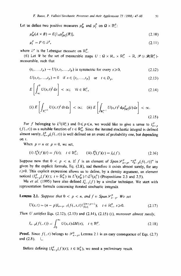
Let us define two positive measures &‘, and &’ on D x R$:

&(A x B) = E[lA&,(B)l, (2.10)

pp = P @ ip, (2.11)

where IJ’ is the Lebesgue measure on R$. (6) Let % be the set of measurable maps I/ : Q x R+ x Rf -+ KY, ,vP @ B([wf )-

measurable, such that

(t1,. . . ,tp> + q&4,. . ., tP) is symmetric for every ~30,

U(s, tl,. . .,tp) = 0 if s E {ti,. . ,tp} or t E D,,

(2.12)

(2.13)

(2.14)

0) E U(s,t)2 dtds 1 < 00; (ii) E U(s, t)2 d/&,(t) ds 1 < cc.

(2.15)

For f belonging to L2(R:) and O< p<n, we would like to give a sense to I& (f (., t)) as a suitable function of t E R$. Since the iterated stochastic integral is defined almost surely, I,“_,( f (., t)) is well defined on an event of probability one, but depending on t.

When p = n or p = 0, we set,

(i) $(f)(t) = f(t); t E @; (ii) C(f)(t) = Mf ). (2.16)

Suppose now that 0 < p < n. If f is an element of SpanYf_,, “Z,“_,(f (., t))” is given by the explicit formula, Eq. (2.8) and therefore it exists almost surely, for any t 30. This explicit expression allows us to define, by a density argument, an element noticed (I:_,(f)(t); t E R$) in L2(&) n L2($) (Propositions 2.3 and 2.5).

Ma et al. (1995) have also defined Z:_,(f) by a similar technique. We start with representation formula concerning iterated stochastic integrals.

Lemma 2.1. Suppose that 0 < p < n, and f E Span c4”& We set

U&t) = (n - p)Z,-,_,(f(.,s,t)l~nsTP-‘); t E iwf, ~30. (2.17)

Then U satisjies Eqs. (2.12) (2.13) and (2.14), (2.15) (i), moreover almost surely,

Lp(f (9 t)) = r

U(s, t)dM(s); t E rw:. (2.18) 0

Proof. Since f (., t) belongs to Yi_,, Lemma 2.1 is an easy consequence of Eqs. (2.7) and (2.8). 0

Before defining (IL_,(f)(t); t E R$), we need a preliminary result.

52 F Russo, P. ValloislStochastic Processes and their Applications 73 (1998) 4768

Lemma 2.2. Suppose that p = 1 and U belongs to 4Y. Then,

cc 03

E [I (J 0 0 U(u)~(4)2d,MMI(t)] = E [l; W>t)24MW(t)d~] .

(2.19)

Proof. Let V+ be the predictable projection of t -+ so” U(s, t) M(s). We know that,

V_(t) = E U(s, t) dM(s)lB,_ I s

= U(& t) M(s). [O,f[

Since U satisfies Eq. (2.13),

UC&t) = w,t)l[o,t[(s) + w, W]t,m[(s).

Consequently,

U(s, t)dM(s) = V_(t) + V+(t), where V+(t) = s

U(s,t)dM(s); t>O.

lw4

We set

2 d,MMl(t), 5*= O” J b(t)2 WfNl(t). 0

V- and t --t Jo t, U(s, t)2 ds being previsible processes, Eq. (2.2) implies that,

E[t-I =E [I” W’dt] = 1” (E [~,$W2ds]) dt,

E[t_] = E [J” (1 0 ,o,t[ U(s, t)2 ds) dMWW] < a.

Let r be the right-inverse of [A&M]. We have,

t+= O” J V+(z(t))2 dt. 0

We observe that (U(s,z(t))l{,(,),,); s 2 0) is 9-measurable. Therefore,

By Fubini theorem we obtain,

Q5+1 =/I b [I” 1,,>~,,,,U(~,T(1))2dfl) ds,

EL<+1 = Ia @ [lo+, W>i)‘WJW~]) ds.

Therefore Eqs. (2.20) and (2.21) tell us that,

lm b[im U(s, t12 dW&fl(t) ])d~=E[Ll+E1t+l < 00.

(2.20)

(2.21)

(2.22)

F. Russo, P. ValloisIStochastic Processes and their Applications 73 (1998) 4768 53

It is clear that,

(J’

0: 2

W,t)dWs) = (V-(t)+ v+(q2 = v_(t)2 + v+(t)2 + 2V_(t)V+(t). 0

By Cauchy-Schwarz inequality we get

E m Iv-(t)v+(t)l d[MMl(t) 1 d (E[4+1E[5-]>“2 < 00. (2.23)

So by Eqs. (2.22), (2.19) is equivalent to

E V_(t)I’+(t)d[M,M](t) 1 = 0. (2.24)

z is the right-inverse of [M,M], consequently,

SI .I

x ~-(~)~+(~>dMW(~)l = V-(~(t)>V+(~(t)) dt,

0 0

and sooo V_(z(t))V+(r(t))dt is the limit (in L](Q)) of ynr when n goes to infinity,

where yn = &’ Ur(t))Mr(r))dt and $&x) = l{,,,) j&l U(s,x)dM(s). We observe that

We can permute “dM(s)” and “ds” (Revuz and Yor, 1991, ex. 5.17, p. 165), we get,

J (s n

Yn = V-(z(t))l{,(,)(,,,),(t)} u(s> r(t>>dt dM(s). lO,nl 0 1

This implies that E[y,] = 0, for every n 3 1. Therefore Eq. (2.24) is satisfied. 0

We are now able to define (&/(f)(t); t E iwf ), by induction on p,f being an element in L2(rW~p). We start with p = 1.

Proposition 2.3. Let n 30. Suppose that f E L2(Ry’) and f (., t) is a symmetric func- tion for any t 20. Then there exists a unique element (Z,‘(f)(t); t 20) in L2(&) n L’(p;) such that

[J cx‘

E Z;(f )(t)2 dW,W(t) (I I [J = E oy Zi(f )(t)‘dt] = n!llf lli+1. (2.25)

If’f E SpanYA,

r;(f)(t) =rn(f(.,t)); v’t>o. (2.26)

Proof. (1) If f E SpanYf, we set IA(f)(t) = Zn(f(.,t)); t>,O. We prove Eq. (2.25) by induction on n when f is an element of Span 9;.

If n = 0, Eq. (2.25) is a consequence of Eqs. (2.16) and (2.2). Assume now that Eq. (2.25) holds. We have to show that Eq. (2.25) is valid if n

is replaced by n + 1.

54 E Russo, P. VaNoislStochastic Processes and their Applications 73 (1998) 4768

Suppose that f E Span 9’:+, Eq. (2.26) and Lemma 2.1 both imply that,

C+*(f)(t) =rn+1(f(.,t)) = lW U(s, t)dws); ws, t) = (n + 1 )Mss(., t)),

(2.27)

where g$(.,t) = f(.,s,t)l$jfl. We claim that U E 4’/, i.e. U satisfies Eq. (2.15)(ii). Notice that gs E SpanYA, therefore using the result at stage n, we have

1 O3 E U(s, t)’ d[M,M](t) = (n + 1)2n! Ilsd-> t>ll; dc J onr IId., Oil: dt G s1‘ o IlfL~,~>ll~d~ < m.

As a result U belongs to %. We are able to apply Lemma 2.2,

E I;+,(f )(02d[MMl(t) = (n + U2n! Iw2 llssM)ll:d~df. I s +

It is now obvious that Eq. (2.25) holds. (2) Let @Span 9’: -+ L2((&+p;)/2); Q(f) = (I,‘(f)(t); ta0). Eq. (2.25) implies

that Cp is an isometry. Therefore @ admits a unique extension to _Y~(iw~ x R+) where

9,2(Rt x R+) = {f E L,2(R”,+‘); f (., t) is a symmetric function V’t>O}.

Let f E LY~(rW~ x IX+). We consider a sequence of functions (fk) belonging to Span YA, converging to f, in Zz(lF!; x R+). It is clear that (I,( fk)) converges to Z,(f) in L’(&) and in L2(pi). Therefore Eq. (2.25) holds. 0

In order to define (Z,‘(f)(t); t E RT) we have to generalize Lemma 2.2.

Lemma 2.4. We suppose that U E %!. Then,

[J (s 00

E ly 0

U(s, +Nr)) * d&@)] G2PE [J,,+, U(s, Q2 d/$,(t) dr]

(2.28)

Proof. We establish this identity by induction on p> 1. If p = 1, Eq. (2.28) is a consequence of Lemma 2.2. Let us assume p > 1. We set,

cj= w J (1 2 U(s, t) w(s) u!: 0 1 &&W

The function U(s, .) is symmetric and U(s, t) vanishes on D,, then,

6=p! O3 J (J CP 0 U(s, t WW) 2 d/&,(0 >

F. Russo, P. ValloislStochastic Processes and their Applications 73 (1998) 4768 55

We decompose the stochastic integral in two parts,

s lx

U(s, t) dM(s) = s uts, t) dws) + 0 [O>l,[ J’ U(s, t) dws),

If/A4

t = (t,,..., tP) E C,. Then,

6 62(6+ + 6- ),

where,

6* = p!

2

V_(x)= W,(v))Ws) 1;,;,'W-bp,i'(~)>

2

V+(x) = W,(v))dWs) 1;,:;'Wd/$&4.

Since V_ is a predictable process,

E[&] = p! s

Oc, E[V_(x>, dx. 0

Using inequality (2.28) at stage p - 1, we get,

where,

Since H is a predictable process,

E Kl{,<,j d.x H, 1 {s<x) W4W(x) 1

.

Consequently,

Let z be the right-inverse of [k&M], then,

E[6+] = p! E[V+W))l ck

We have,

J (J > 2

v+(e)) = co-1 IGbM

U(s,(u,r(x)))l~,~~~~,(;:[(,)dM(s) d$i,lW

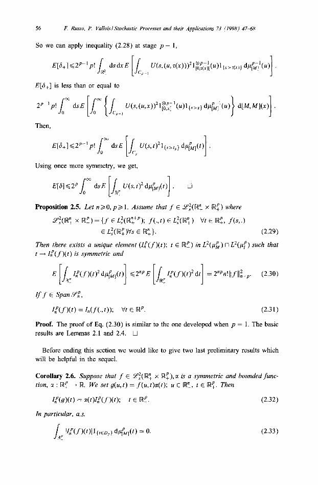
56 F. Russo, P. ValloislStochastic Processes and their Applications 73 (1998) 4768

So we can apply inequality (2.28) at stage p - 1,

E[6+] is less than or equal to

Then,

WJ)21~,,,p) d$&(t) 1 .

Using once more symmetry, we get,

Proposition 2.5. Let n 20, pa 1. Assume that f E Zf(R”, x rW$ ) where

s:<rwn, X lR$> = {f E L,2(lQ”fP); f(.,t) E L,2(rw:) vt E rw$, f(s,.)

E L~(Rfc)Vs E R”,}. (2.29)

Then there exists a unique element (Z/‘(f)(t); t E R$) in L2(&) n L2(&‘) such that t --f I{(f)(t) is symmetric and

E 4f’(f)(t)2 d/&,(t) ] G2 E np [if 4’Yf)(t)2 dt] = 2”‘n! kfll~+,. (2.30)

If f E SpanY,P,

JfXf)(t) = Jl(f(.,t)); vt E RP. (2.31)

Proof. The proof of Eq. (2.30) is similar to the one developed when p = 1. The basic results are Lemmas 2.1 and 2.4. 0

Before ending this section we would like to give two last preliminary results which will be helpful in the sequel.

Corollary 2.6. Suppose that f E Y;(rW; x R$), a is a symmetric and bounded func- tion, CI : Rf + R. We set g(u, t) = f(u, t)cl(t); u E RF, t E Rf. Then

Ii(g)(t) = Nt)Jf(f)(t); t E @. (2.32)

In particular, a.~.

J I4W-)(t)l I{ED~) d$&) = 0. (2.33) a:

F. Russo, P. Valloisl Stochastic Processes and their Applications 73 (1998) 4768 51

Lemma 2.7. Let f be in E 6”,2(rWt x Rf). Then

E R(f)(t) I d$&) Ilf(., t)lln dc

where C = 2nJ’i2v%,

3. An extension of Kabanov formula

We start with the first extension of Kabanov formula.

Theorem 3.1. Let n3 1,f E 5?i(rW”,-’ x rW+) and g E L2(rW+). Then

s O3 I~,‘_I(f)(t>s(t)l dW,Ml(t) below to L’,

0

MfYl(9> = hI+1(f @ 9) + n SW

I,‘-l(f)(t)g(t)d[M,Ml(t). 0

Remark 3.2. (1) Recall that (Z,_,(f)(t); t B 0) is the element of defined by Proposition 2.3.

(2.34)

(3.1)

(3.2)

L2(&) r--I L=(d)

(2) If M is the Brownian motion, then [h&M](t) = (M,M) (t) = t; Eq. (3.2) is a par- ticular case of formula 15.3 of Dellacherie et al. (1992), (p. 212), or Surgailis (1984).

Proof of Theorem 3.1. (1) Let us introduce

5= s

O” I4-,(f)WsWl Wf+fl(t). 0

Using successively Kunita-Watanabe and Schwarz inequalities, we have,

(3.3)

where,

51= O” s

g(t)= 4MW(t), t2= Ml J’ L,WW= WWfl(t).

0 0

Obviously, g E L2(rW+) and Eq. (2.2) imply E[~I] < co, moreover E[52] < 00 is a direct consequence of Proposition 2.3.

(2) For the proof of Eq. (3.2), it is sufficient to consider a symmetric function f, and g of the following type:

g = l]zJ], f = l]a,,b,] @ " ' @ l]a,,b,] on CR,

where Odcl < /I, OQal < bl < a2 < b2 < ... < a, < b,. Using linearity, we only have to consider,

(3.4)

B < a1 or b, < c(,

c( = ai, p= bi for some i E {l,...,n}.

(*I

c**>

58 E Russo, P. ValloislStochastic Processes and their Applications 73 (1998) 4768

Assume that (Ir) is realized; by Eq. (2.7), Z,+i(S @g) = Zn(f)Zi(g) and the integral in the right-hand side of Eq. (3.2) is equal to 0. It is clear that Eq. (3.2) holds.

Let us study the case (kk). We have,

Al(f) = m((wh) - M(Q)), 11(g) =M(bi) -M(Q),

where

Pi = n (M(bj) -M(Uj)).

j=l, j#i

On Gfl, an easy calculation shows that

(f~,>= @ l]a,,b,] @ l]a;,bJ @ . . . @ ll%,b*]).

Then,

Zn+l (f @ g) = 2n!Pi I (M(s-) - M(R)) w(S). la,,bJ

If t E]Ui, bi],

So Eq. (3.2) reduces to,

(3.5)

(M(bi) - M(Ui))’ = 2 1

(M(s-) -“(&))~(s) la,,hl

This ends the proof of Theorem 3.1. 0

Kabanov (1975), considered a compensated Poisson measure based on a measured space (r, a, A), such that T is a locally compact space with a countable basis and II is a Radon measure. Assume that T = Iw+, 1 is the Lebesgue measure on [w+, and the Poisson measure is defined by a random point measure. The compensated Poisson measure is associated with M, where M(t) = N(t) - t; t 2 0, and (N(t); t > 0) is a standard Poisson process with jumps equal to 1. In this setting Kabanov (1975) proved,

zn(f)zl(S> = In+l(f @S> + kzn(f *j 9) + nzn-l(f x 913 (3.6) j=l

where f ELS([W;), gEL2(R+), (f*jg)EL2(Rt) forevelyjE{l,...,n},

(f *j g>(tl>. . ‘3 tn> =f(tl,...,tn)g(tj),

(f x s)(tl,...,tn-1) = J mf(t t , l,...,tn-l)dt)dt.

0

F Russo, P. ValloislStochastic Processes and their Applications 73 (1998) 4768 59

We notice that in Eq. (3.2) we do not need to suppose that f *j g E L2(Rt), for every i E {l,..., n}. We observe that Eq. (3.6) is a particular case of Eq. (3.2) since

MW(t) = N(t).

Corollary 3.3. Assume that n 2 1, f E Lf(R:),g E L2(R+) and f *j g E L2(R;)for every j E { 1,. . ,n} and M is a compensated Poisson process. Then Eq. (3.6) holds.

Proof. By Aztma and Yor (1991, ex. 5.17, p. 165), we have,

Z,-l(f‘ x 9) = g(t)Z,‘-,(f)(t)dt.

We notice that

j=l

Moreover [h&M](t) = N(t) where N is a classical Poisson process; so by Theorem 3.1, Eq. (3.6) is equivalent to,

(3.7)

In order to check Eq. (3.7), it is sufficient to take elementary functions f and g defined by Eq. (3.4). As in the previous proof, we introduce cases (*) and (**). In (*), the two sides of Eq. (3.7) are equal to 0. If (**) holds,

s(tYd-~(f>(t)dWt) = (n - 1 Y J

pi dM(t) Id+1

= (n - l)! fi(A4(b,) - M(Uj)), j=l

where Pi is defined by Eq. (3.5). By a direct calculation, we obtain immediately,

Zn(f*ig)=(n-l)!fi(M(h,)-M(CZj)). 0 j=l

Notations. (1) Let f E L2( I%~‘“), n 2 0, p 3 0. We suppose that f(~, .) is a symmetric function, for any s in RF. We set

Z,“(.Z-) = Z,“(f), (3.8)

where 7 : WJ’ + R,f(., t) is the symmetrization of f(., t),t E R$. As a result f(s,.) and T(., t) are symmetric functions, for any s E rWt and t E RT. This means that f E 2$X”, x R$?). Moreover (Z:(f)(t); t E lR$) belongs to L2(&) n L*(pr) and

E Z,p(f)(t)* d&,,(t) 1 62”Pn!llfll~+p~ (3.9)

&,, being the random measure on rWT defined by Eq. (2.9).

60 E Russo. P. Valloisl Stochastic Processes and their Applications 73 (1998) 47-68

It is not difficult to check that Z{(f) verifies Eqs. (2.32) and (2.33). (2) Assume that O<p<n,p<m, f : RF 4 R, g : RT ---t R. We set,

(f xp g)(u, 4 t) = f (u, Mv, t>9

where t = (tt,. . . ,t,), u = (u~+~, . . . , un), v = (vp+l,. . . , v,). By definition, f xp g : R!~?“-p + R, and f x0 g = f ~3 g. If f and g are elements of Li(R;), respectively Lz([w$), then (f xp g)(u, v, .) is

symmetric; consequently Z:+m_2p(f xP g) is defined by Eq. (3.8).

The main result of this section is the following.

Theorem 3.4. Letn>l, m31, l<p<mAn, f EL,~(IW”,), gE@IWT). Then

s I~~+,_2p(f xp g)(t)1 G&,(t) belongs to L’. (3.10) %?

zR,,_,,(f xp g)(t)&&(t).

(3.11)

Remarks. (1) If M is the Brownian motion, Eq. (3.11) is the formula given by Surgailis (1984) and Dellacherie et al. (1992), (formula 15.3, p. 212).

(2) Let us examine the case m = 1. Eq. (3.11) reduces to

s

00 Mf >b(g) = L,l(f @ 9) + n I,-,(f x1 s>(t)WM(0

0

The function f x1 g verifies: (f XI g)(u, t) = f(u, t)g(t). Therefore Corollary 2.6 tells

us that Zi_ I (f x I g)(t) = s(tY,‘_, (f )(t). C onsequently, Eq. (3.11) corresponds exactly to Eq. (3.2).

Proof of Theorem 3.4. (1) We start with Eq. (3.10). By definition Z,&,_zP (f x p g) = I,“,,_,,($), @(., t) denotes the symmetrization of

the function: (u, v) -+ (f xp g)(u, u, t) = f (u, t)g(v, t). Lemma 2.7 implies

E k%-,,(f XP s)(t)1 dqt&) II~C,t)lln--m--2p dt.

But,

IIb@7 OIL--m--2p G Il(f xp g)(., t)lln--m-2p = Ilf (.> t)Lpllg(., t)llm-p.

I R: IlIC/Wlln-m-zpd= Ilf Ilnllsllm.

E I&n-,,(f xp s)(t)l h&(t) 1 d cllf Ilnllsllm~ (3.12)

F. Russo, P. ValloislStochastic Processes and their Applications 73 (1998) 47-68 61

(2) In order to check Eq. (3.11), we proceed by induction on k = m A n. If k = 1, m = 1 or n = 1, we have already noticed that Eq. (3.11) corresponds to Eq. (3.2). We now assume that m A n = k + 1 and Eq. (3.11) holds. By symmetry, we can suppose that n = k + 1 and man. Moreover by Eq. (3.12), it is sufficient to consider g E 9: and f =fo, where,

J’o = l]a,,b,] 8 . . . @ ]]a,,h,],

and 0 < al < bl < . . . < a,, < b,. Let fh = l]n,,b,] @ . @ l]an_,,bn_,], f' = Jk and c( = l]O&,]. Through an easy

calculation it follows that

f=(fG>, (3.13)

Z&Z-) = Z,-l(f’)Zl(cc), (3.14)

f’(.,.s)~(.s) = 0; Vs>O. (3.15)

By Theorem 3.1, we have,

Zl(aYds) = L+i(s LX E> + m s M GI(S)z~-,(g)(S)d[M,Ml(s). 0

g being an element of Y$ Z:_,(g)(s) = Z,_i(g(.,s)). Multiplying both sides by Zn_i(f’) we obtain

Zn(f)Zm(g) = Yl + Y2,

where.

y2 = m r

a(s)Z,-l(s(.,s))Z,-l(f’)d[M,Ml(s). 0

Since(n-l)A(m+l)=n-1 and(m-l)A(n-l)=n-l,wehave,

n-l

Yl = c p> y2 = &p)> p =L+m(f'@(s~~)),

p=o p=l

c~~(.,t) is the symmetrization of(f’ xp (gxa))(.,t>; l<p<n - 1,

y$f’ = m(p - l)! (;I ; ) (“,-: ) s,. Zn+m-2p((P*)(t)d~~](t),

(~2(.,t) is the symmetrization of a(tp)(g(.,tp) x~_~ f’)(.,rl, . . ..tp-1).

t = (tl,...,tp).

62 E Russo, P. ValloisIStochastic Processes and their Applications 73 (1998) 47-68

(i) Let 1 <pQn - 1. The function t -+ Zf+,_z,(cpi)(t) is symmetric, and as. equal to 0 on D, with respect to ,L&,, therefore,

(P) = (n - l)!(m + l)! Y1 (n - 1 - p)!(m + 1 - p)! s c, ~,+,_,,(cpi )(t) d$.&).

We easily check,

where (a c$., t)) is the symmetrization of the function tx@g(., t), t = (11,. . . , tp), .?i =

(t1 ,...,ti-l,ti+l,...,tp).

Using Eq. (3.15), we obtain

f’(., t) CG g-s-4, t) = m ,’ :; Pf’(., t) @ (a @-zJ)).

Since

(f’ Xp (sTu))(., t) = f’(., t) 8 (gTa)(., t),

and

PZG2 = &5-p, = p”,xC , (3.16)

then,

(P) = Yl (n - 1 - p)!(m - p)! .I

4z+m--2p(N., t)) d$&); 1 <pGn - 1. (3.17) c,

(n - l)!m!

h(., t) being equal to the symmetrization of f’(., t) ~3 g(., t) @ a. (ii) We now reduce y2 (P); 1~ p dn. By the same way, we obtain,

(P) = (n - l)!m! Y2

s (n - pY(m - PY C, ~n+m--2~(H(.,t))~l(tp)d~~~,(t),

where

H_( ., t) is the symmetrization of g(., t) ~3 f’(., tl, . . , t,_l ); t = (tl, . . . , tP).

(iii) We set,

l<p<n,

where

(pP(., t) is the symmetrization of (f x p g)(., t); 1 < p < n.

If ldpdn, we have,

$P) = n!m!

(n - p)!(m - p)! s bz+m--Zp(vp)(t)d$&).

C,

F RU.YSO. P. ValloislStochastic Processes and their Applications 73 (1998) 4768 63

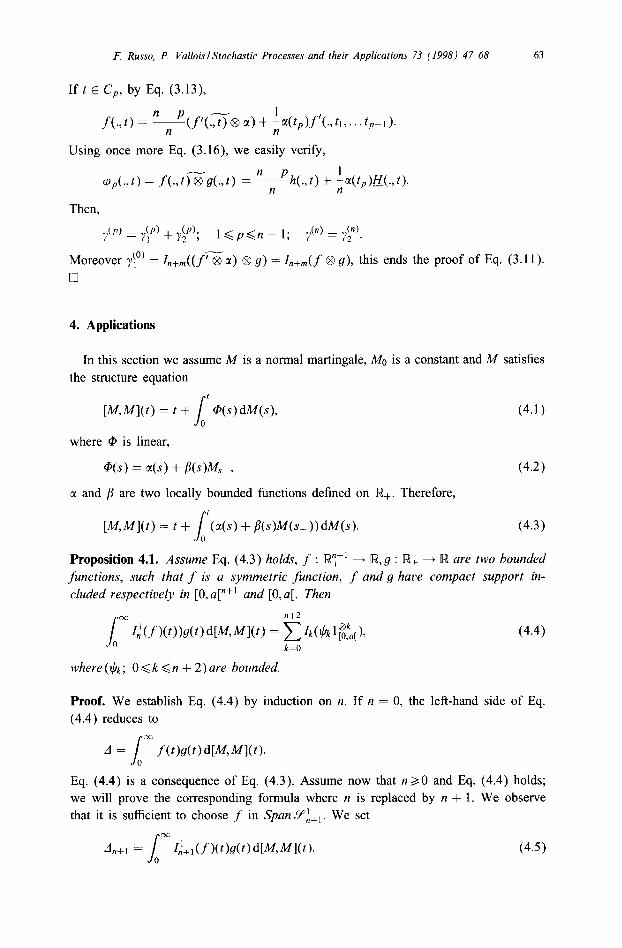
If t E C,, by Eq. (3.13),

f(.,t) = ~(f’(.X@a)+ ia(t,)f’(..t, ,... t,-I).

Using once more Eq. (3.16) we easily verify,

q,(.,t) = f(.,~)EG(.J) = -h(., t) + Aa(tp)H(., t). n

Then,

y(p) = y(,p) + @‘; 1 <p<n - 1; y(“) = $‘.

Moreover ~(10’ = In+m((fGa) @ g) = In+m(f @ g), this ends the proof of Eq. (3.11). 0

4. Applications

In this section we assume M is a normal martingale, Ma is a constant and M satisfies the structure equation

s I

[M,M](t) = t + @(s) U(S)> 0

(4.1)

where Q, is linear,

Q(s) = a(s) + P(s)K,

c( and a are two locally bounded functions defined on R+. Therefore,

(4.2)

[MM](t) = t + s

f(a(s) + j(s)M(s-))dM(s). (4.3) 0

Proposition 4.1. Assume Eq. (4.3) holds, f : rWy’+’ + R,g : R+ -+ R are two bounded functions, such that f is a symmetric function, f and g have compact support in- cluded respectively in [O,a[“+’ and [O,a[. Then

k=O

(4.4)

where ($k; 0 < k < n + 2) are bounded.

Proof. We establish Eq. (4.4) by induction on n. If n = 0, the left-hand side of Eq. (4.4) reduces to

.I

‘3c1 A= f(t)g(t) dPCW(t).

0

Eq. (4.4) is a consequence of Eq. (4.3). Assume now that n20 and Eq. (4.4) holds; we will prove the corresponding formula where n is replaced by n + 1. We observe that it is sufficient to choose f in Span Yi,, . We set

A n+l = r,‘+,(f )(tMt)dMW(t). (4.5)

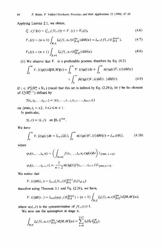
64 F. Russo, P. ValloislStochastic Processes and their Applications 73 (1998) 4768

Applying Lemma 2.1, we obtain,

G+*(f)@) = ~,‘+i(f(J)) = V-(t) + V+(l),

V_(t) = (n + 1) s

Mf(.,U? Ql$,) M(u) = &+1(f(., wgy )Y lO>t[

(4.6)

(4.7)

V+(t)=(n+l) J z,(f(.,u,t)l~~~[)dM(U). (4.8) I@4

(1) We observe that V- is a predictable process, therefore by Eq. (4.3)

/I V-(t)dt)dWM(t) = .I” VMt)dt + lrn 4t)s(t)v-(t)dWt)

+ J ox B(t)g(t)V-(t)M(t-)dM(t). (4.9)

If y r~ Zf(Ry x R,) (recall that this set is defined by Eq. (2.29)), let 7 be the element of L~(rW~+‘) defined by

Y(~l~~2~~~~r~~+l)~~(~l~~~~~~i-1~~i+l~~~~r~m+l~ti)

on {IIMXjZj = ti}; 1 di<m + 1. In particular,

y(.,t) = y(.,t) on [0, t[@“.

We have

.Im V-(fMt)dt =4,+1(E), Jrn 4t)s(t)v-(t>cwt) = L+2Gin (4.10) 0 0

where

cPl(h ) . . . ) tn, u) = (I f (t1, . . ..~u.s)ds)ds l{maxz t,<uj, lw4 >

(P2~h,...,Gl+1,~) = ~~(‘)g(‘)f(tl,...,~~+l,~)l~~~~,*~<~~.

We notice that

v-(tw(f-) = L+1(f (.,Ol[,,,[ @l+l Z1(1[0,1[) 1

therefore using Theorem 3.1 and Eq. (2.26), we have,

v-(t)w-) = L+2M.,t)l;~;*) + (n + 1) J

z,(f(.,u,t)l~~~,)d[M,Ml(u), lo>t[

where (ps(., t) is the symmetrization of f (., t) 64 1. We now use the assumption at stage n,

I ni2

lO>G Z,(f(.,u,t)l~~*,)d[M,Ml(u) = ~‘dBk’$;r).

k=O

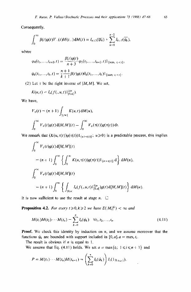
F Russo, P. Vallois IStochastic Processes and their Applications 73 (1998) 4768 65

Consequently,

s O”

0 P(t)g(t)V-(t)M(t-)dMt) = bl+3m + ~zk+m

k=O

where

B(t)s(t) (P4(t1,.. *,tu+z,t> = ___ n+3 (P3(tlr...,tn+2,t)l{max, r,<t}>

n+l $k/k(h,...,tk,t) = - k+ ,P(t)g(t)ok(tl,...,t,)l{,,, r,<t}.

(2) Let z be the right inverse of [M,M]. We set,

K(u,t) = In(f(.>U,t)l;~U[)~

We have,

V+(Q=(n+l) J’

K(u, t) M(u), It@1

.Im v+(t)s(t) dW,Ml(t) = S’ V+($t)M~(t)) dt.

0 0

We remark that (K(u,z(t))g(z(t))l{,,,(,)}; ZJ 3 0) is a predictable process, this implies

sm ~+(Mt)WWl(t)

0

=(n+l) O” s {S

Oc K(u,z(t))g(z(t))l{,>,(,)} d 0 0

s

lx

~+(tMt)W>W(t) 0

=(n+l) O” S {I 0 IO,4

r,(f(.,u,t)l~~~,>s(t)d[M,Ml(t) ~WU). I

It is now sufficient to use the result at stage n. 0

Proposition 4.2. For every t 2 0, k 2 2 we have E((M Ik) < co and

hf(tl)hf(t2)...M(tn) = kI,($k, ~tlrt2,...,tn.

k=O

(4.11)

Proof. We check this identity by induction on n, and we assume moreover that the functions $k are bounded with support included in [O,a],a = maXi ti.

The result is obvious if n is equal to 1. We assume that Eq. (4.11) holds. We set a = max{t,; 1 6 i <n + 1) and

P = M(t, ). . .M(tn)M(tn+l) =

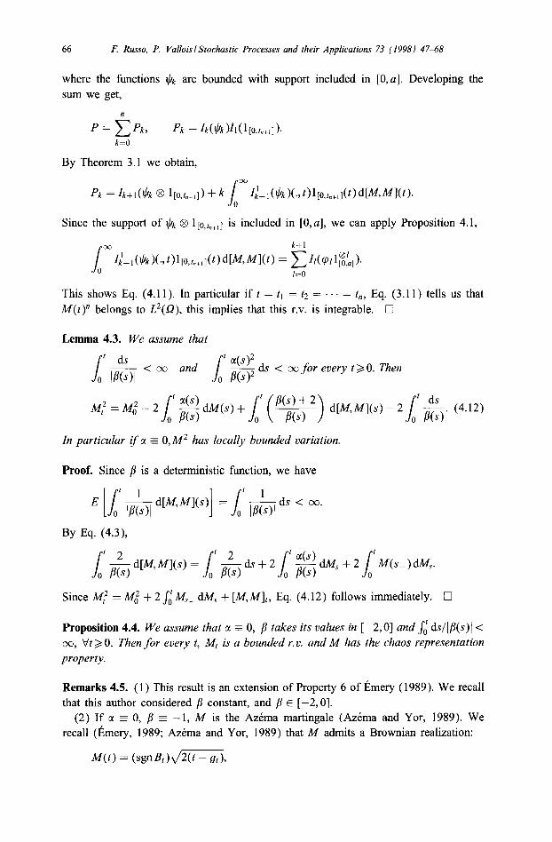
66 F. Russo, P. Vallois I Stochastic Processes and their Applications 73 (1998) 4768

where the functions sum we get,

n

p = CPk, k=o

pk = Ik($k’kb(][O,t,+,]).

By Theorem 3.1 we obtain,

$,, are bounded with support included in [0, a]. Developing the

pk = Ik+l ($k @ l[o,t,+,]) + k J

Ikl-l(~k)‘k)(.,t)l[o,t,+,](t)d[M,Ml(t). 0

Since the support of $k @ 1 [~+,l is included in [O,a], we can apply Proposition 4.1,

1;

k+l

0 zkl-,(~kk)(.,t)l[o,t,+,,(t)d[M,Ml(t) = ~hhl;,$).

I=0

This shows Eq. (4.11). In particular if t = ti = t2 = . . 1 = tn, Eq. (3.11) tells us that M(t)” belongs to L2(s2), this implies that this r.v. is integrable. ??

Lemma 4.3. We assume that t ds s- < co and s

f cqsy

0 IP(s)l - ds < cc for every t 2 0. Then

0 P(s12

lq=A4,2-2 -dM(s)+l (w) d[M,M,(s)-2l&. (4.12)

In particular if cl = 0,M2 has locally bounded variation.

Proof. Since ,!I is a deterministic function, we have

BY Eq. (4.31,

Since M: = kfi + 2 $M,_ dk& + [M,M],, Eq. (4.12) follows immediately. 0

Proposition 4.4. We assume that LY = 0, /I takes its values in [-2,0] and sd ds/I/3(s)l< 00, Vt 3 0. Then for every t, Mt is a bounded r.v. and A4 has the chaos representation property.

Remarks 4.5. (1) This result is an extension of Property 6 of Emery (1989). We recall that this author considered j3 constant, and p E [-2,0].

(2) If a = 0, /I = - 1, A4 is the Azema martingale (Aztma and Yor, 1989). We recall (Emery, 1989; Azema and Yor, 1989) that M admits a Brownian realization:

F. Russo, P. ValloisIStochastic Processes and their Applications 73 (1998) 4768 67

where (Bt; t >O) is a usual Brownian motion, started at 0,

gt = sup{u<t; B, = 0).

If LX z 0, and fl = -2, A4 is the parabolic martingale (Emery, 1989, p. 79). Once more this process has a Brownian interpretation:

where T(a) = inf (~30, lBsl = u}. By definition A4(t)2 = t. We can easily observe that for these two examples, M(t)* has locally bounded

variation, and M(t) is a bounded r.v. (3) If Mt = &B(e(&)); t>O) where (e(t); t>,O) is the inverse of the range

process of B, then Vallois (1995) showed that M is a parabolic martingale.

Proof of Proposition 4.4. Our proof is closely related to the one given by Emery. Since c( = 0, and (p(s) + 2)/p(s) d 0, then

O<Mf<M,2- tds s 0 P(s)’

This implies that the T.v. Mf is bounded. Consequently, exp(iu cl=, AjMt, ) is the limit in L’ of polynomial Qk(M(tl),. . . ,M(t,,)). It is sufficient to use Proposition 4.2. 0

5. Unlinked Reference

Dermoune et al. 1990; Nualart et al. 1990; Privault, 1994; Russo et al., 1993; Russo et al., 1995; Skorohod, 1975.

Acknowledgements

The financial support of F. Russo has been partially granted by a Human Capital and Mobility fellowship of the European Union; this author is grateful for the warm and stimulating atmosphere in BIBOS Research Center of Universitat Bielefeld. The authors would like to thank the referee, whose remarks enabled us to give a more precise definition of Z{(f).

References

Attal, S., Bmety, M., 1994. Equations de structure pour des martingales vectorielles Sdminaire de Probabilites XXVIII, Lectures Notes in Math., vol. 1583. Springer, Berlin, pp. 256-278.

Azema, J., Yor, M., 1989. Etude d’une martingale remarquable. Stminaire de Probabilitbs XXIII, Lectures Notes in Math., vol. 1372. Springer, Berlin, pp. 88-130.

Dermoune, A., 1995. Chaotic&y on a stochastic interval [O,T]. Seminaire de Probabilitds XXIX, Lectures Notes in Math., vol. 1613. Springer, Berlin, pp. 117-124.

Dermoune, A., K&e, P., Wu, L., 1990. Calcul stochastique non-adapt& par rapport a la mesure aleatoire de Poisson. Sbminaire de Probabilites XXII, Lectures Notes in Math., vol. 1321. Springer, Berlin, pp. 4777484.

68 E Russo, P. ValloisIStochastic Processes and their Applications 73 (1998) 47~58

Dellacherie, C., Meyer, P.A., Maisonneuve, B., 1992. Chap. XVII 1 XXIV Processus de Markov (fin). Complement de Calcul Stochastique. Hermann, Paris.

Emery, M., 1989. On the Azema martingale. Seminaire de Probabilitb XXIII, Lectures Notes in Math., vol. 1372. Springer, Berlin, pp. 66-87.

Ito, K. (1951). Multiple Wiener integral. J. Math., Sot. Japan, 3, 157-169. Kabanov, Yu.M. (1975). On extended stochastic integrals. Theory Probab. Appl., xX(4), 710-722. Ma, J., Protter, P., San Martin, J., 1995. Anticipating integrals for a class of martingales. Technical report

95-39, Perdue University. Meyer, P.A., 1976. Un tours sur les integrales stochastiques. Seminaire de Probabilites X, Lectures Notes

in Math., vol. 511. Springer, Berlin, pp. 245400. Meyer, P.A., 1986. Elements de probabilitis quantiques. Seminaire de Probabilites XX, Lectures Notes in

Math., vol. 1204. Springer, Berlin, pp. 186312. Nualart, D., Vives, J., 1990. Anticipative calculus for the Poisson process based on the Fock space. Seminaire

de Probabilites XXIV, Lectures Notes in Math., vol. 1426. Springer, Berlin, pp. 154-165. Privault, N., 1994. Chaotic and variational calculus in discrete and continuous time for the Poisson process.

Stochast. Stochast. Rep. 51, 83-109. Revuz, D., Yor, M., 1991, Continuous Martingales and Brownian Motion. Springer, Berlin. Russo, F., Vallois, P., 1993. Forward, backward and symmetric stochastic integration. Probab. Theory Rel.

Fields 97, 40342 1. Russo, F. and P. Vallois (1995). The generalized covariation process and ItB formula. Stochast. Process.

Appl., 59, 81-104. Shigekawa, I. (1980). Derivatives of Wiener fimctionals and absolute continuity of induced measures. J.

Math., Kyoto Univ., 20(2), 263-289. Skorohod, A.V., 1975. On a generalization of a stochastic integral. Theory Probab. Appl. XX, 219-233. Surgailis, D. (1984). On multiple Poisson stochastic integrals and associated Markov semi-groups. Probab.

Math., Statist., 3(2), 217-239. Tudor, C., 1996. A product formula for multiple Poisson-Ito integrals. Rev. Roumaine Math Pures Appl.,

to appear. Vallois, P. (1995). Decomposing the Brownian path via the range process. Stochast. Process. Appl., 55,

21 l-226.