Embed Size (px)
Citation preview
1 June 2018 | ESMA50-162-215
Product Intervention Analysis Measures on Contracts for Differences

ESMA • CS 60747 – 103 rue de Grenelle • 75345 Paris Cedex 07 • France • Tel. +33 (0) 1 58 36 43 21 • www.esma.europa.eu
2

3
Table of contents
1 Executive summary ........................................................................................................ 5
2 Analysis of likely impact of different options .................................................................... 6
2.1 Product description and overview of the retail market .............................................. 6
2.1.1 Key product features ........................................................................................ 6
2.1.2 Common characteristics of the retail market ..................................................... 7
2.2 Summary of problem to be addressed by intervention measures ............................ 7
2.2.1 Geographical scope of problem ........................................................................ 7
2.2.2 Market failure analysis ...................................................................................... 8
2.3 Summary of intervention measures ......................................................................... 8
2.4 Systemic context and market efficiency ................................................................... 8
2.5 Impact on firms and investors .................................................................................. 9
2.5.1 Baseline scenario ............................................................................................. 9
2.5.2 Evidence base .................................................................................................10
2.5.3 Analysis of high-level options ..........................................................................10
2.5.4 Analysis of detailed options .............................................................................14
Margin close-out protection ...........................................................................................14
Initial margin protection .................................................................................................17
Negative balance protection ..........................................................................................21
Restriction on incentives ................................................................................................24
Risk warning ..................................................................................................................25
Treatment of cryptocurrency CFDs ................................................................................26
3 Simulation results informing leverage limits ...................................................................29
3.1 Methodology...........................................................................................................30
3.1.1 Alternative approaches ....................................................................................30
3.2 Assumptions and focus of simulation exercise .......................................................31
3.2.1 Assumptions ...................................................................................................31
3.2.2 Focus ..............................................................................................................32
3.3 Results ...................................................................................................................34
3.4 Sensitivity analysis .................................................................................................38
4 Annexes ........................................................................................................................42
Annex I – Core results for individual assets ......................................................................42
Annex II – Detailed methodology ......................................................................................49

4
4.1.1 Raw data .........................................................................................................49
4.1.2 Adjusting the raw data for the purpose of simulating returns ...........................49
4.1.3 MCO assumption ............................................................................................50
Annex III – Evidence relevant to choice of assumptions and focus ...................................52
4.1.4 Range of durations presented .........................................................................52
4.1.5 Asset selection ................................................................................................58

5
1 Executive summary
This document summarises and analyses relevant evidence in relation to the provision of
contracts for differences (CFDs) to retail investors. This document complements the
European Securities and Markets Authority Decision of 22 May 2018 to temporarily restrict
contracts for differences in the Union in accordance with Article 40 of Regulation (EU) No
600/2014 of the European Parliament and of the Council (the Decision), providing additional
detail. This document sets out:
analysis of the impact that different intervention options in relation to CFDs would
be expected to have on investors and on firms; and
a study of the effect of leverage on investor positions in CFDs, which has
informed the setting of initial margin protection (commonly referred to as
‘leverage limits’).
In designing the product intervention measures through extended information-gathering and
discussion with National Competent Authorities (NCAs), ESMA considered different
alternatives. Section 2 of this document describes the different intervention options
considered and examines the expected impact of each option. Some impacts are described
in qualitative terms, while in other cases quantitative information is available.
On 18 January 2018, ESMA issued a call for evidence on possible intervention measures,
to gather additional information. Key evidence and data from the call for evidence are
reflected in the analysis of section 2 of this document.
As studies by NCAs have shown – consistent with academic research and as also
acknowledged by some CFD providers – high leverage causes poor outcomes for investors.
This is why ESMA, in its work, has paid particular attention to leverage, as well as other
aspects of the marketing, distribution or sale of CFDs. High leverage can be detrimental in
three ways. First, because leverage magnifies the costs of investment – such as spreads,
commissions or financing charges – relative to margin, at very high leverage investment
costs deplete a large share of an investor’s margin. Second, leverage amplifies investor
losses and returns. The higher the leverage, the smaller the adverse price movement
required to deplete much or all of an investor’s margin. Third, leverage is associated with
higher volumes of trading by investors, increasing trading costs via repeated entering and
exiting of positions. ESMA simulated CFD returns based on several years of market data to
examine the first two of these sources of detriment. Section 3 presents simulation results of
the probability with which an investor’s margin reaches half its initial value, under certain
assumptions. The assumptions and parameters used in the model take into account
available statistics and data from firms. The results help ensure that leverage limits across
asset classes are consistent and evidence-based.

6
2 Analysis of likely impact of different options
1. This section of the document:
describes what CFDs are and describes the retail market for CFDs;
explains the key features of the problem that has led ESMA to take action;
summarises the intervention measures that ESMA is introducing;
examines any potential impact the different intervention options could have on the wider
financial system; and
analyses the expected direct impact of the different options on investors and on firms.
2. The definitive specification of what CFDs are, of the intervention measures and of the problem
addressed is in the Decision alongside which this document is published.1
2.1 Product description and overview of the retail market
2.1.1 Key product features
3. This analysis relates to CFDs that are cash settled derivative contracts the purpose of which is
to give the holder an exposure, which can be long or short, to fluctuations in the price, level or
value of an underlying. These CFDs include, inter alia, rolling spot forex products and financial
spread bets.
4. CFDs are often traded on margin, i.e. leveraged. For a leveraged CFD, a given percentage
change in the price of the underlying asset implies a larger percentage change in the amount
invested. Box 1 gives a numerical example.
Box 1: example of a CFD traded on margin
As an example, consider a long CFD, which has as underlying the price of gold. If the price of
gold rises during the time the investor holds the CFD, then the value of the CFD increases.
Suppose that the notional value (total exposure) of the CFD contract is €10,000, and the investor
deposits 5% of this as initial margin, i.e. €500. In this case, the CFD is leveraged at 20:1.
A 3% increase in the price of gold results in a total exposure of €10,300. If the investor sells the
CFD at this point, then (neglecting spreads and transaction fees, and assuming the price of the
underlying is correctly reported by the provider) the investor receives a return of €300, i.e. a 60%
return on the initial margin. On the other hand, if the price of gold falls 5% from its value at the
start of the contract, the investor loses the entire margin.
If the CFD is instead leveraged at 100:1, the initial margin on a CFD contract with notional value
of €10,000 is €100. A 3% increase in the price of gold determines a 300% return on initial margin.
On the other hand, a 1% decrease in the price of gold from its value at the start of the contract
will deplete the investor’s entire initial margin.
1 European Securities and Markets Authority Decision of 22 May 2018 to temporarily restrict contracts for differences in the Union in accordance with Article 40 of Regulation (EU) No 600/2014 of the European Parliament and of the Council.
7
2.1.2 Common characteristics of the retail market
5. CFDs are cash-settled derivative contracts and unlike some other products, such as options,
typically do not have a predetermined expiry. Retail investors, to whom these products have
been massively offered through online channels across the EU predominantly on a non-advised
basis, usually hold CFDs as short term investments, in some cases as short as a few minutes,
ranging up to several months.
6. Many firms offer CFDs on a wide range of underlying assets, including currency pairs, equities,
equity indices and commodities. The assets offered and the prominence with which they are
listed on providers’ websites may change over time. For instance, in 2017 several providers
started offering CFDs on cryptocurrencies. Providers earn a profit from selling CFDs to retail
investors through spreads, commissions and/or fixed fees. Different providers may have
different business models, with some hedging their entire exposure and others, to varying
extents, leaving positions unhedged. Additionally, some firms may net client positions before
hedging. NCAs have observed that there are greater conflicts of interest associated when firms
do not hedge their client’s exposure, which may negatively impact retail investors through
poorer quality of execution or higher fees.
7. In all cases, the investor has exposure (whether long or short) to movements in the price of the
underlying asset and will pay some form of spread, commission or fee.
2.2 Summary of problem to be addressed by intervention measures
8. The problem identified in connection with the provision of CFDs to retail investors stems from
three related issues, as follows.
(i) Retail investors, on average, have received poor outcomes from investing in CFDs. In
particular, a significant majority of retail investors in CFDs have lost money from investing
in CFDs, a phenomenon observed across countries and over time. Evidence from NCAs,
as mentioned in the Decision, is that that in recent years a clear majority of client accounts
have typically lost money on their investments, with substantial average losses per client,
though with precise figures ranging between different jurisdictions.
(ii) In addition to yielding negative net returns on average, the products are highly risky, with a
greater risk of significant losses the greater the leverage. Some of the underlying risks can
result in severe detriment, e.g. the investor owing significant sums of money to a firm as a
result of adverse price movements.
(iii) In many cases, retail investors do not properly understand the risks underlying the products
in question and the costs of investing. The products are complex, and this complexity is one
reason why many investors lack a proper understanding of the associated risks and costs.
Retail investors without a proper understanding of the risks are encouraged to trade CFDs
by aggressive marketing techniques. Retail investors’ understanding is also hampered by
a lack of sufficiently clear accompanying information.
2.2.1 Geographical scope of problem
9. The issue has an EU-wide impact on retail investor protection, as evidenced by investor
outcomes in many Member States. In many cases, retail customers trade CFDs with providers
that operate cross-border. Numbers of cross-border providers increased from 2016 to 2017
8
according to data from two authorities that supervise many such firms, the Cyprus Securities
and Exchange Commission (CySEC) and the UK Financial Conduct Authority (FCA). Many
authorities have taken initiatives to address problems in their own jurisdictions using both
MiFID-derived conduct of business rules and, in some cases, restrictions on the products, their
marketing and commercialisation. However, poor consumer outcomes persist.
2.2.2 Market failure analysis
10. The problem is due in part to informational asymmetries, which may lead consumers to make
decisions that are not in their interests ex ante, evidenced as follows.
A clear majority of investors lose money, despite the fact that most aim to realise positive
returns. This indicates that retail investors as a group overestimate the net returns they are
likely to receive.
In many cases, retail investors do not properly understand the risks underlying the products
in question, as NCAs have observed in the course of doing supervision and as evidenced
by consumer complaints. Some of the underlying risks can result in severe detriment, e.g.
the investor owing significant sums of money to a firm as a result of adverse price
movements.
2.3 Summary of intervention measures
11. In the Decision, ESMA is imposing temporary (three-month) restrictions on the provision of
CFDs to retail investors.
12. The temporary restrictions in question are summarised in broad terms as follows:
1) Margin close out protection. If the margin allocated to a CFD trading account (including initial
margin and any variation margin allocated to the position) by a retail investor falls to less
than 50% of the minimum required initial margin of the open CFD positions, the provider
must close out the position(s) on terms most favourable to the client.
2) Initial margin protection. Retail investors opening CFD positions are required to post
minimum required initial margin, with this minimum requirement dependent on the
underlying asset.
3) Negative balance protection. The liability of a retail investor in respect of a CFD trading
account is limited to payments already made into the account and any uncrystallised profits
on open positions within the account.
4) Restriction on incentives. Firms are prohibited from providing retail investors with any
incentives in relation to the marketing, sale or distribution of CFDs other than
research/information tools.
5) Risk warning. Information sent by firms to retail investors in relation to the marketing, sale
and distribution of CFDs must be accompanied by a risk warning.
2.4 Systemic context and market efficiency
13. There is no evidence of systemic risk from restricting or prohibiting the provision of CFDs to
retail clients in the EU. Although firms providing CFDs to retail clients often hedge some or all
of their exposure in institutional markets, notional volume in the retail market for CFDs is a very

9
small fraction of that for products that CFD providers are likely to use to hedge exposure,
namely derivative contracts such as futures. For this reason, the intervention measures are
expected to have no discernible impact on prices or liquidity of underlying assets or of other
derivative contracts.
14. An order-of-magnitude estimate of volumes in the retail CFD market across the EU is sufficient
to establish this conclusion. Research by the International Organization of Securities
Commissions (IOSCO) published in December 2016 reports notional traded volumes in rolling
spot FX and CFDs for retail investors resident in France to be at least EUR 200 billion per year,
with at least 4 million trades taking place per year.2 An order-of-magnitude estimate can be
obtained for the EU-wide market simply by scaling according to the relative GDP of France
compared to the EU as a whole, suggesting estimated traded notional volumes of the order of
EUR 1 trillion in the retail market for CFDs and rolling spot forex contracts.3 This figure is likely
to be significantly higher than open interest notional, as the typical duration of retail CFD
contracts is short. Even so, the figure is a very small fraction of total open interest notional for
foreign exchange derivatives in the EU, which stands in excess of EUR 100 trillion according
to EMIR data.4 Open interest notional in equity derivatives in the EU is around EUR 35 trillion,
while that in commodities derivatives is around EUR 9 trillion.
2.5 Impact on firms and investors
15. The following part of section 2 deals with costs and benefits that the relevant options considered
by ESMA in developing the temporary restrictions listed above would be likely to have on
investors and on firms.5 The analysis includes both qualitative and quantitative evidence.
2.5.1 Baseline scenario
16. The baseline scenario against which the impacts of the intervention options are assessed is
the regulatory regime to which the market is subject prior to the commencement of the
2 See page 11 of the Report on the IOSCO Survey on Retail OTC Leveraged Products, the final version of which was published in December 2016 and is available at https://www.iosco.org/library/pubdocs/pdf/IOSCOPD550.pdf. Aggregate traded nominal value (including leverage) in these two product families was reported to be at least EUR 200bn per year, while according to the same source at least 4 million trades reportedly took place per year.
3 France accounted for 15% of EU GDP as of 2016, based on Eurostat data, suggesting an estimate of around EUR 1.3 trillion. The equivalent figure using banking sector assets is around EUR 1 trillion, based on European Banking Federation data. A different estimate can be obtained based on figures provided IG Group in response to the call for evidence assessing the French market for retail CFDs to be around 5% of the EU market for retail CFDs, in terms of client numbers. Scaling by this figure would imply traded notional volumes of the order of EUR 4 trillion in the retail market for CFDs. The large difference between the estimates reflects that they are simply order-of-magnitude calculations. For both estimates, traded notional volumes of retail CFDs are likely to be significantly higher than open interest notional, as the typical duration of retail CFD contracts is short. Nonetheless, these volumes are a very small fraction of total open interest notional for foreign exchange derivatives in the EU.
4 Based on EMIR data as of 24 February 2017. For related information and discussion see ESMA Report on Trends, Risks and Vulnerabilities No. 2, 2017, “EU derivatives markets – a first-time overview”. 5 Impacts on investors should be interpreted while bearing in mind the objective to address the identified significant investor protection concerns. In particular, it is important to note that aggregate monetary total costs and benefits, where obtainable, do not necessarily equate to aggregate detriment, e.g. in the following respects. (i) Some consumers may not expect certain costs, or understand the risk that the costs will materialise. If the costs do then materialise, the resulting detriment may be greater than if the consumers had anticipated the risk. (ii) The wealth and liquidity of consumers bearing costs also have a bearing on detriment. For example, a consumer whose losses exceed his or her cash balances with a firm and is unable to settle his or her account is likely to suffer considerably more detriment than an investor suffering a loss of the same size but which is covered by his or her cash balances. (iii) The distribution of costs on consumers is relevant to detriment. Other things equal, if a given aggregate loss falls on a smaller number of investors, this may cause more overall detriment than the same aggregate loss spread over a larger number of investors.

10
measures in question. In particular, firms are assumed in the baseline scenario to be subject
to the requirements of MiFID II / MiFIR, all other applicable EU Directives and Regulations and
all national rules in force. For example, the baseline scenario includes the prohibition on the
commercialisation of certain complex products (including CFDs) in Belgium and the restrictions
on the provision of CFDs to retail clients in countries such as Cyprus, France, Germany and
Poland as these policies are expected to be in place when the temporary ESMA restrictions
come into force.
17. When assessing each one of measures 1, 2 and 3, the baseline scenario includes the other
two of the three measures. For example, margin close out protection (measure 1) and initial
margin protection (measure 2) together reduce the risk of an investor suffering a negative
balance. However, they do not prevent this from happening under extreme market conditions.
Rather, this risk is addressed by measure 3. In this way, measure 3 operates as a backstop;
the analysis below reflects this, considering the marginal impact of measure 3 taking measures
1 and 2 as given.
2.5.2 Evidence base
18. In respect of the impact of the measures on retail investors, the evidence base includes detailed
analysis using quantitative modelling techniques in addition to academic research and
qualitative analysis. In respect of the costs and benefits to firms, the evidence is mostly
qualitative. Firms however did provide some quantitative estimates of expected initial and
ongoing implementation costs which have been analysed and taken into account.
19. Survey data as reported by firms responding to the call for evidence and data on investors’
reasons for opening CFD positions are cited in relation to the assessment of costs and benefits
to retail investors and firms. ESMA does not have information on how the survey answers were
elicited or on the selection of survey samples. Similar qualifications apply to survey data
provided by firms on clients’ stated plans as to whether to invest in future using non-EU
platforms. Estimates of market size and reported investor returns provided by firms have not
been independently assessed or verified. Data on the durations of trades, received directly from
a firm and from NCAs, were used to inform the focus and interpretation of the data-based
simulations of the impact of leverage and margin close-out protection on investor returns. One
limitation of these data is that they relate to the distributions of trade durations and not to the
distribution of typical holding durations over the population of investors.
2.5.3 Analysis of high-level options
20. Section 2.5.3 summarises the high-level intervention options considered, such as whether to
impose a prohibition on the marketing, sale or distribution of CFDs to retail clients. The selected
high-level option was to impose restrictions on the provision of CFDs to lessen the risks
investors face and to improve investors’ understanding of those risks that remain. Section 2.5.4
then examines the costs and benefits associated with the different detailed sub-options
stemming from the selected high-level option.
11
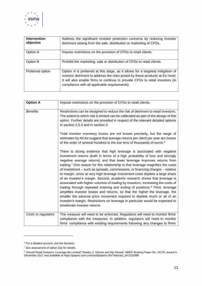
Intervention objective
Address the significant investor protection concerns by reducing investor
detriment arising from the sale, distribution or marketing of CFDs.
Option A Impose restrictions on the provision of CFDs to retail clients.
Option B Prohibit the marketing, sale or distribution of CFDs to retail clients.
Preferred option Option A is preferred at this stage, as it allows for a targeted mitigation of
investor detriment to address the risks posed by these products at EU level.
It will also enable firms to continue to provide CFDs to retail investors (in
compliance with all applicable requirements).
Option A Impose restrictions on the provision of CFDs to retail clients.
Benefits Restrictions can be designed to reduce the risk of detriment to retail investors.
The extent to which risk is limited can be calibrated as part of the design of this
option. Further details are provided in respect of the relevant detailed options
in section 2.5.4 and in section 3.
Total investor monetary losses are not known precisely, but the range of
estimates by NCAs suggest that average returns per client per year are losses
of the order of several hundred to the low tens of thousands of euros.6
There is strong evidence that high leverage is associated with negative
investment returns (both in terms of a high probability of loss and strongly
negative average returns) and that lower leverage improves returns from
trading.7 One reason for this relationship is that leverage magnifies the costs
of investment – such as spreads, commissions, or financing charges – relative
to margin, since at very high leverage investment costs deplete a large share
of an investor’s margin. Second, academic research shows that leverage is
associated with higher volumes of trading by investors, increasing the costs of
trading through repeated entering and exiting of positions.8 Third, leverage
amplifies investor losses and returns, so that the higher the leverage, the
smaller the adverse price movement required to deplete much or all of an
investor’s margin. Restrictions on leverage in particular would be expected to
ameliorate investor returns.
Costs to regulators The measure will need to be enforced. Regulators will need to monitor firms’
compliance with the measures. In addition, regulators will need to monitor
firms’ compliance with existing requirements following any changes to firms’
6 For a detailed account, see the Decision.
7 See assessment of option 2(a) for details.
8 Should Retail Investors' Leverage Be Limited? Rawley Z. Heimer and Alp Simsek. NBER Working Paper No. 24176, issued in December 2017 and available at https://papers.ssrn.com/sol3/papers.cfm?abstract_id=2150980

12
business models and online platforms as a result of the measures. This could
cause higher costs for regulators than option B.
Compliance costs Firms providing CFDs to retail investors would need to amend existing
systems. Descriptions of specific compliance costs are provided in respect of
the relevant detailed options in section 2.5.4.
Other costs ESMA’s assessment is that there would be an overall limited increase in the
costs faced by retail investors using CFDs arising from leverage limits. In many
cases, retail investors continuing to trade CFDs will be required to post
additional margin. For example, in information provided in response to the call
for evidence, IG Group stated that, in the second half of 2017, 57% of its EU
retail clients had undertaken trades at leverage exceeding the leverage limits
that ESMA set out (and which ESMA is now implementing). However, the
opportunity cost to investors of holding additional cash is limited, as posting
additional margin should reduce typical overnight financing fees charged by
firms, which are typically 1-2 percentage points above the prime rate.
Some retail investors may cease trading or limit their trading of CFDs as they
are no longer able to afford the margin necessary to open a CFD position.
Other retail investors, in contrast, would be able to ‘opt up’ to professional
status. Among the minority of investors who trade profitably on a sustained
basis, those lowering their notional exposure may see reduced returns
compared to the baseline scenario as leverage limits lower returns from
profitable positions. Overall, however, retail investors are expected to lose less
money on average and reduce the volatility of returns on individual positions.
Retail investors who cease trading will no longer lose money from trading
these products.
Firms responding to the call for evidence argued that some investors may
choose to use providers based outside the EU as a result of leverage
restrictions, limiting the protection provided by the measures. IG Group
reported results from a survey of its clients in Japan (where leverage limits on
CFDs in currency pairs are 25:1) that one third of such clients used a provider
based outside Japan for some trades. ESMA notes that any product
intervention measures would expose the risk that investors may seek providers
from non-EU jurisdictions; the risk of some arbitrage with some third country
jurisdiction is therefore unavoidable. In this respect, ESMA also notes that a
third country regime has been included in MiFID II to this effect and this will be
able to contribute to addressing this risk. ESMA also notes that, as the situation
stands, the EU as a whole has not adopted any restrictions and firms based in
the EU may therefore attract business from those jurisdictions that have
adopted restrictions to protect investors. In this respect, the introduction of
certain restrictions in the EU is therefore consistent with the approach of other
jurisdictions which have felt the need to take some measures to address
investor protection concerns arising from the offering of CFDs.
Additionally, a minority of retail investors benefit from using CFDs to hedge a
portfolio in the baseline scenario. Such investors are expected to continue to
hedge their portfolios under option A, either via CFDs or via other hedging
13
tools. For example, retail investors have access to a wide range of products
on-exchange, such as interest rate swaps or vanilla options that can be tailored
to a specific hedging need. Retail investors wishing to use CFDs for hedging
purposes will be allowed to continue doing so; the measures will require more
cash to open CFD positions. As discussed above, the opportunity cost of
holding additional cash is limited.
Firms indicated that applying the restrictions could involve significant
implementation costs, depending on the design of the rules.
Firms are also expected to experience lower revenues and some firms may
choose to cease trading altogether.
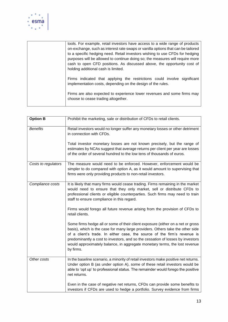
Option B Prohibit the marketing, sale or distribution of CFDs to retail clients.
Benefits Retail investors would no longer suffer any monetary losses or other detriment
in connection with CFDs.
Total investor monetary losses are not known precisely, but the range of
estimates by NCAs suggest that average returns per client per year are losses
of the order of several hundred to the low tens of thousands of euros.
Costs to regulators The measure would need to be enforced. However, enforcement would be
simpler to do compared with option A, as it would amount to supervising that
firms were only providing products to non-retail investors.
Compliance costs It is likely that many firms would cease trading. Firms remaining in the market
would need to ensure that they only market, sell or distribute CFDs to
professional clients or eligible counterparties. Such firms may need to train
staff to ensure compliance in this regard.
Firms would forego all future revenue arising from the provision of CFDs to
retail clients.
Some firms hedge all or some of their client exposure (either on a net or gross
basis), which is the case for many large providers. Others take the other side
of a client’s trade. In either case, the source of the firm’s revenue is
predominantly a cost to investors, and so the cessation of losses by investors
would approximately balance, in aggregate monetary terms, the lost revenue
by firms.
Other costs In the baseline scenario, a minority of retail investors make positive net returns.
Under option B (as under option A), some of these retail investors would be
able to ‘opt up’ to professional status. The remainder would forego the positive
net returns.
Even in the case of negative net returns, CFDs can provide some benefits to
investors if CFDs are used to hedge a portfolio. Survey evidence from firms

14
suggests a minority of investors use CFDs for this purpose. The costs of
removing the possibility for retail investors to use CFDs for hedging purposes
are mitigated by the existence of other tools, such as interest rate swaps or
vanilla options, which can be tailored to a specific hedging need.
2.5.4 Analysis of detailed options
21. Section 2.5.4 examines the costs and benefits associated with different options for the design
of restrictions on the provision of CFDs to retail clients.
22. One issue raised in the call for evidence was the treatment of CFDs with cryptocurrency
underlying. Reflecting this, intervention options relating specifically to CFDs with cryptocurrency
underlying treated as a separate question in the analysis below. Among these options, ESMA
has decided, at this stage, to impose leverage limits specific to cryptocurrency CFDs as part of
its temporary restrictions on the provision of CFDs to retail investors. As such, the analysis of
the general intervention options concerning initial margin protection also extends to
cryptocurrency CFDs.
23. Detailed results of the simulations used to inform the design of the (selected) options 1(a) and
2(a) are set out in section 3.
Margin close-out protection
Intervention
objective
Address the significant concerns of detrimental outcomes for investors by
introducing consistent margin close out practices among CFD providers.
Option 1(a) Margin close-out protection on an account basis at 50% of minimum required
initial margin. Under this option, a firm is required to close out one or more of
an investor’s positions on the best possible terms for the investor if the value
of the margin in a CFD trading account falls below 50% of the total minimum
initial margin required for all CFDs in the account.
Option 1(b) Margin close-out protection on a position basis at 50% of minimum required
initial margin. Under this option, a firm is required to close out an investor’s
position on the best possible terms for the investor if the value of the margin in
a particular position falls below 50% of the minimum initial margin required for
the position.
Option 1(c) No margin close-out protection
Preferred option For the reasons explained in this document and in the Decision, it is necessary
to introduce margin close-out protection to mitigate the risk of retail clients’
losses. Option 1(c) therefore cannot be pursued.
Option 1(a) is preferred at this stage because it is less burdensome and costly
for firms and is better-suited than 1(b) at enabling investors with multi-asset
portfolios to benefit from asset diversification, while at the same time, it

15
achieves a sufficient safeguard across CFD providers. Additionally, option 1(a)
is likely to be significantly quicker to implement than 1(b).
Option 1(a) Margin close-out protection on an account basis at 50% of minimum required
initial margin.
Benefits Margin close-out protection limits clients’ losses in normal trading
circumstances. To avoid the setting of the margin close-out protection by firms
to a very low percentage that would risk defeating the objective of the measure,
a specific percentage (50%) is introduced. This standardises the percentage
at which CFD providers are required to close out positions and allow a
consistent application of margin close-out practices by CFD providers.
Many investors hold only a single CFD position with a provider at any given
time. For these investors, options 1(a) and 1(b) offer the same protection.
In general, the leverage limits being introduced are designed to ensure that
automatic close-out happens infrequently. As a result, for those investors with
more than one CFD in their account, there are likely to be only modest
differences in outcomes between the two options. While it is not possible to
quantify precisely any such differences, a per account rule should reduce the
frequency of automatic close-out compared to a per position rule. Modern
portfolio theory suggests that investors benefit from lower overall risk if they
have diversified portfolios, in which case a lower probability of a position being
closed out is beneficial. Additionally, a reduced probability of close-out reduces
possible costs from re-entering positions.
One firm responding to the call for evidence, XTB Brokers, stated that leverage
limits would encourage clients to hold a position for longer period of time. While
the firm is correct that overnight financing rates are a cost of multi-day
positions, to the extent that longer holdings become relatively more attractive
to investors compared with very frequent short-duration trading, leverage limits
are expected to reduce overall costs to investors through less frequent
payment of spreads and commissions. This is because investors bear costs in
entering or re-entering positions, which are typically larger than financing costs
applied over a few days. Indeed, one example of longer term trading that
provides better investor outcomes (according to data from IG Group in its
response to the call for evidence) is the carry trade, where investors receive
positive net overnight interest payments.
In accordance with responses to the call for evidence, a close-out rule per
account would be less expensive to firms than a per position rule. Responses
to the call for evidence suggest that many existing investors are familiar with a
per account rule. The choice of a 50% threshold is likely to strike a reasonable
balance between providing protection against the depletion of account funds
and the potential for negative outcomes from frequent close-outs not at the
investor’s request.

16
Costs to regulators The measure would need to be enforced, requiring monitoring of CFD offerings
by national authorities.
Compliance costs Firms would be required to close out positions that would not necessarily
otherwise have been closed out. Providing this service is likely to involve
limited costs for the firm. Indeed margin close-out protection per account is
already applied by a number of firms who responded to the call for evidence
whereas requiring the implementation of margin allocation on a per position
basis would imply additional initial and ongoing costs.
Other costs In general, the leverage limits being introduced are designed to ensure that
automatic close-out happens only rarely. As a result, for those investors with
more than one CFD in their account, there are likely to be only modest
differences in outcomes between the two options. While it is not possible to
quantify precisely any such differences, a per account rule – option 1(a) –
should reduce the frequency of automatic close-out compared to a per position
rule, i.e. option 1(b). Modern portfolio theory suggests that investors benefit
from lower overall risk if they have diversified portfolios, in which case a lower
probability of a position being closed out is beneficial. Additionally, a reduced
probability of close out reduces possible costs from re-entering positions.
Option 1(b) Margin close-out protection on a position basis at 50% of minimum required
initial margin
Benefits Margin close-out protection limits clients’ losses in normal trading
circumstances. The standardisation of the percentage at which CFD
providers are required to close out a client’s open CFD allows a consistent
application of margin close-out practices by CFD providers. The resulting
rule is clear and simple for retail investors to understand.
Applying the rule on a per position basis would be beneficial to consumers
who view each position as an individual investment. This rule could be
simpler to understand for retail clients as positions would be treated on an
individual basis.
Costs to regulators The measure would need to be enforced, requiring monitoring of CFD
offerings by national authorities.
Compliance costs
Firms would be required to close out positions that would not necessarily
otherwise have been closed out. Providing this service is likely to involve
costs for the firm, both one-off costs (i.e. transitional costs from implementing
new systems and introducing new terms and conditions) and ongoing costs
(i.e. costs involved in monitoring positions and closing them out as required).
One-off costs are likely to be higher under option 1(b) than option 1(a)
because in the baseline scenario, standard market practice is to operate
margin close-out on an account basis rather than a position basis. IG Group
estimated, as reported in responding to the call for evidence, that changing

17
computer systems would require around 10,000 person-days of work by IT
specialists. IG Group estimated an associated cost of around GBP 3.5 million
for that firm, implying a cost of around GBP 350 per day per IT specialist
employed. CMC Markets estimated a total cost of around GBP 700,000 to
GBP 800,000, or around 900 person-days.
In assessing the magnitude of ongoing costs to firms, it is important to note
that initial margin protection has been designed such that automated close-
out happens for fewer than 5% of positions open for at least a day (in the
case of all underlying assets except equities, where longer time horizons are
more relevant). Because some traders execute large numbers of much
shorter-duration trades, and the simulation neglects the possibility that
clients top up or close out their positions intra-day, ESMA expects the actual
incidence of close-out due to the operation of the intervention option to be
substantially fewer than 5% of trades. This limits the scope for significant
ongoing costs for firms in implementing margin close-out.
Other costs Many investors hold only a single CFD position with a provider at any given
time. For these investors, options 1(a) and 1(b) offer the same protection.
As described in more detail in the assessment of option 1(a) above, the
difference in likely costs to investors between the two options is in practice
likely to be small.
Initial margin protection
Intervention
objective
Address the significant investor protection concerns by improving overall
investor outcomes
Option 2(a) Initial margin protection by class of underlying asset. (Regarding the treatment
of cryptocurrency CFDs in particular, see options 6(a) to 6(c) below.)
Option 2(b) Single level of initial margin protection for any underlying.
Option 2(c) No initial margin protection.
Preferred option For the reasons explained in this document and in the CFD Decision, the
setting of an initial margin protection is essential to address the significant
investor protection concerns arising from the sale, distribution or marketing of
CFDs to retail clients. Option 2(c) cannot therefore be pursued.
Option 2(a) is preferred because it allows for consistent mitigation of investor
risk across classes of assets which display substantially different historical
volatility.

18
Option 2(a) Initial margin protection by class of underlying asset
Benefits Given any price change in the underlying, the magnitude of an investor’s gross
return on his or her margin increases linearly with the leverage of the position.
As a result, high levels of leverage increase the risk of losing significant
amounts of deposited funds (while also increasing the upside). Minimum initial
margin requirements – i.e. requiring that an investor initially post margin at
least equal to a set percentage of the notional value of a contract – reduce
leverage and therefore limit the risk of significant losses.
Research by NCAs and other institutions indicates an inverse relationship
between leverage and average investor returns.9 Important reasons for this
are that a given spread or charge on a CFD position comprises a larger
proportion of initial margin at higher leverage, and the cumulative impact of
transaction fees associated with higher volumes of trading.
Additionally, if an investor is closed out automatically, rather than at the
investor’s own instigation, the investor may wish to re-enter the position by
posting more margin, at which point the investor incurs costs from spreads or
other charges. This is a potential cost to investors (and conversely, a source
of profit for firms). Initial margin protection reduces the probability with which
close-out happens compared with the baseline, for a given level of margin
close-out protection, as typical margin requirements in the industry are less
stringent than those of option 2(a).
Initial margin protection for different classes of underlying has been set
according to the variability of the underlying using a simulation model to assess
the likelihood of a client losing 50% of their initial investment over an
appropriate holding period. Specifically, ESMA undertook a quantitative
simulation of the distribution of returns an investor in a single CFD might
expect to receive at different leverage levels. The starting point of the
simulation was several years of daily market price data for various underlying
types commonly used in CFDs sold to retail clients.10 The analysis considered
a single CFD that is automatically closed out if the margin reaches 50% of its
initial value. The simulated probability with which close-out occurs is increasing
in the given leverage. A metric examined was the probability of (automatic)
close-out as a function of leverage. This metric allows for leverage limits to be
9 In a 2014 study, the AMF found that investor performance decreased in leverage and in the number of trades. See “Study of investment performance of individuals trading in CFDs and forex in France”, available at http://www.amf-france.org/technique/multimedia?docId=workspace%3A%2F%2FSpacesStore%2F9bf2caa8-1ce4-4832-85f4-4dffcace8644&famille=PIECE_JOINTE. Recent academic research provides causal evidence that leverage constraints have reduced the underperformance of individual investors in the US. The data relate to retail traders of foreign exchange in the US and Europe, and the identification strategy exploits the introduction by the US Commodity Futures Trading Commission of leverage limits into the US retail market. The limits in question were 50:1 for major currency pairs and 20:1 for minor pairs. See Should Retail Investors' Leverage Be Limited? Rawley Z. Heimer and Alp Simsek. NBER Working Paper No. 24176, issued in December 2017 and available at https://papers.ssrn.com/sol3/papers.cfm?abstract_id=2150980. 10 Market price data was sourced from Thomson Reuters for all assets except for the Nikkei stock index and for cryptocurrencies, for which data were provided by an NCA. In most cases, approximately 10 years of data were used. Exceptions were some equities, for which price data were only available for the period starting at the relevant initial public offering, and cryptocurrencies, for which price data were only available following the launch of the cryptocurrency.

19
set based on a consistent assessment of the risk of detriment across different
classes of underlying asset.
Statistics on the distributions of CFD holding periods (using data collected by
NCAs) show considerable heterogeneity between firms. For CFDs with
underlying other than equities, according to most firms for which data was
gathered, a majority of trades were intra-day. The share of retail investors
holding such positions is not clear from the data, however. For instance, some
investors conduct many trades of extremely short duration, speculating on
price movements over minutes or hours. Initial margin protection is not
primarily designed to reduce per-trade risks for these investors, but addresses
such risks for those (likely to form a significant share of the population) who
hold positions for at least one day or, in the case of equities, several days, as
data indicate that equity holdings are typical several times those of other asset
classes 11
To provide a consistent reference point, ESMA then simulated what leverage
would lead to the automatic close-out of a position with a 5% probability for
different underlying assets. For example, among commodities CFDs, oil and
gold are both commonly traded by retail investors, but simulations indicate that
the leverage implying a 5% probability of mandatory close-out for CFDs in gold
is around twice that of CFDs in oil and substantially higher than most other
(less commonly-traded) commodities. The initial margin protection for CFDs in
gold is accordingly lower (i.e. permitted initial leverage is higher) than for those
in oil and other commodities.
The initial margin protection is designed to mitigate consumer detriment in two
ways, which are relevant to the calibration of the measure. First, initial margin
protection is expected to improve average outcomes for investors, both per-
trade and per-account. As set out in the analysis of option A above, academic
evidence indicates that lower leverage limits (i.e. higher initial margin
requirements) improve such average outcomes. Second, the initial margin
protection is intended to reduce the risk of substantial per-trade losses
occurring. In ESMA's assessment, the levels of initial margin protection being
introduced are required to address these investor protection concerns. More
stringent initial margin protection would further improve average outcomes and
further lessen the risk of substantial per-trade losses occurring compared with
the initial margin protection being implemented. Less stringent initial margin
protection would improve average outcomes and reduce the risk of substantial
per-trade losses compared to the baseline scenario, but to a lesser extent.
Costs to regulators The measure would need to be enforced, requiring monitoring of CFD offerings
by national authorities.
11 Accordingly, simulations were carried out for durations of 1 day, 2 days, 3 days, 4 days and 5 days. For CFDs with underlying
assets other than equities, in setting the initial margin protection the 1 day duration was used. In the case of equities CFDs, data
suggest that holdings are typically longer than for other assets, and consideration was given especially to the upper end of the
range of durations for which results were obtained.
20
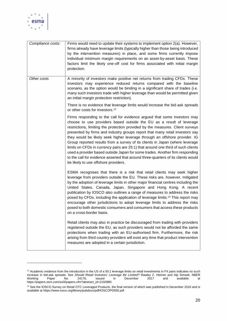
Compliance costs:
Firms would need to update their systems to implement option 2(a). However,
firms already have leverage limits (typically higher than those being introduced
by the intervention measures) in place, and some firms currently impose
individual minimum margin requirements on an asset-by-asset basis. These
factors limit the likely one-off cost for firms associated with initial margin
protection.
Other costs A minority of investors make positive net returns from trading CFDs. These
investors may experience reduced returns compared with the baseline
scenario, as the option would be binding in a significant share of trades (i.e.
many such investors trade with higher leverage than would be permitted given
an initial margin protection restriction).
There is no evidence that leverage limits would increase the bid-ask spreads
or other costs for investors.12
Firms responding to the call for evidence argued that some investors may
choose to use providers based outside the EU as a result of leverage
restrictions, limiting the protection provided by the measures. Client surveys
presented by firms and industry groups report that many retail investors say
they would be likely seek higher leverage through an offshore provider. IG
Group reported results from a survey of its clients in Japan (where leverage
limits on CFDs in currency pairs are 25:1) that around one third of such clients
used a provider based outside Japan for some trades. Another firm responding
to the call for evidence asserted that around three-quarters of its clients would
be likely to use offshore providers.
ESMA recognises that there is a risk that retail clients may seek higher
leverage from providers outside the EU. These risks are, however, mitigated
by the adoption of leverage limits in other major financial centres including the
United States, Canada, Japan, Singapore and Hong Kong. A recent
publication by IOSCO also outlines a range of measures to address the risks
posed by CFDs, including the application of leverage limits.13 This report may
encourage other jurisdictions to adopt leverage limits to address the risks
posed to both domestic consumers and consumers that access these products
on a cross-border basis.
Retail clients may also in practice be discouraged from trading with providers
registered outside the EU, as such providers would not be afforded the same
protections when trading with an EU-authorised firm. Furthermore, the risk
arising from third country providers will exist any time that product intervention
measures are adopted in a certain jurisdiction.
12 Academic evidence from the introduction in the US of a 50:1 leverage limits on retail investments in FX pairs indicates no such increase in bid-ask spreads. See Should Retail Investors' Leverage Be Limited? Rawley Z. Heimer and Alp Simsek. NBER Working Paper No. 24176, issued in December 2017 and available at https://papers.ssrn.com/sol3/papers.cfm?abstract_id=2150980.
13 See the IOSCO Survey on Retail OTC Leveraged Products, the final version of which was published in December 2016 and is available at https://www.iosco.org/library/pubdocs/pdf/IOSCOPD550.pdf.

21
Option 2(b) Single level of initial margin protection for any underlying.
Benefits As explained in the assessment of the previous option, minimum initial margin
requirements reduce investor leverage and therefore limit the risk of significant
losses. Academic research and NCAs’ studies indicate a clear inverse
relationship between leverage and average investor returns.
Additionally, if an investor is closed out automatically, rather than at the
investor’s own instigation, the investor may wish to re-enter the position by
posting more margin, at which point the investor incurs costs from spreads or
other charges. This is a potential cost to investors (and conversely, a source
of profit for firms).
The level of initial margin protection could be informed using the same
approach as option 2(a), but based on a single basket of different assets. As
this basket would not be a representative portfolio, but rather a combination of
underlying assets that are individually commonly-traded, the resulting limit
could not be interpreted as a simulation of the probability of a given level of
loss, however, unlike with option 2(a).
Costs to regulators The measure would need to be enforced, requiring monitoring of CFD offerings
by national authorities.
Compliance costs Firms would need to update their systems to implement option 2(b). However,
firms already have leverage limits (typically higher than those being
introduced) in place, and some firms currently impose individual minimum
initial margin requirements on an asset-by-asset basis. These factors limit the
likely one-off cost for firms associated with initial margin protection.
Other costs A minority of investors make positive net returns from trading CFDs. These
investors may experience reduced returns compared with the baseline
scenario, as the option would be binding in a significant share of trades (i.e.
many such investors trade with higher leverage than would be permitted given
an initial margin protection restriction).
Negative balance protection
24. Measure 1 (margin close-out) implies that an investor can still suffer a negative balance on a
position or a trading account in extreme market conditions. Measure 2 (leverage limits) lessens
the expected impact of such extreme conditions by restricting leverage. In this way, measure 3
(negative balance protection) operates as a backstop to measures 1 and 2, and is considered
as such in the analysis below.
25. The analysis for the options connected with this measure is primarily qualitative. A precise
estimate of the direct benefit to investors from limiting losses in the case of an extreme market
event is not feasible, due to the fact that such events are by nature unknown in advance and

22
varying in their effects. In the case of the Swiss Franc event, some investors had a negative
balance running to tens of thousands of euros, many times the cash they had deposited with
their CFD provider.14 This suggests that on an individual basis the realised benefit of negative
balance protection (options 3(a), 3(b) and 3(c)) can be large, though such benefits are very rare
occurrences.
Intervention
objective
Address the significant investor protection concern arising from the very high
detriment to some investors from rare and extreme market events
Option 3(a) Negative balance protection on an account basis
Option 3(b) Negative balance protection on a position basis
Option 3(c) No negative balance protection.
Preferred option For the reasons explained in this document and in the Decision, it is necessary
to limit retail clients’ exposure to losses in extreme market circumstances.
Option 3 (c), therefore, cannot be pursued.
Option 3(a) is preferred because, like option 3(b), it prevents the severe
detriment associated with negative account balances following extreme market
conditions. ESMA does not consider that the costs imposed on firms (which
would probably be partly and indirectly met by investors) by requiring a greater
transfer of risk from firms to investors than that implied by option 3(a) are
warranted by the corresponding marginal benefits to investors in extreme
market conditions.
Option 3(a) Negative balance protection on an account basis
Benefits An important risk of major consumer detriment that arises in the absence of
negative balance protection is the potential for an investor to owe money to a
firm as a result of extreme market conditions. Such a situation is especially
detrimental for investors without considerable liquid wealth.15 Options 3(a) and
3(b) both prevent this situation from occurring. Beyond this, option 3(b)
minimises the direct costs to consumers that can arise in extreme market
conditions. Consequently, the direct benefit to investors from option 3(a),
which materialises in cases of rare and extreme market events, is less than
option 3(b).
14 ‘Swiss franc event’ refers to the sudden appreciation in the Swiss franc against the Euro, of the order of 15%, on the morning of Thursday 15 January 2015.
15 The detriment caused in such a situation was evident in relation to the Swiss franc event, where some investors unwittingly became liable for tens of thousands of euros, sums they were unable to pay.

23
Costs to regulator The measure would need to be enforced, requiring monitoring of CFD offerings
by national authorities.
Compliance costs
Firms would need to update their systems to implement option 3(a).
Economically, negative balance protection measures involve a transfer of risk
from consumers to firms. To manage this risk, firms bear additional capital
costs and/or costs of hedging the risk with other counterparties.
These additional costs may cause some firms to leave the market. The costs
may also to some extent be passed back to consumers as a whole through
higher spreads or charges on CFDs. Consequently, the incidence of the costs
imposed by the measure is very difficult to estimate with any precision, but
some of the costs would likely be borne by firms and some by investors.
Notably, many of the costs arising to any firms which exit the market for retail
CFDs as a result of negative balance protection, in the form of foregone profits
(but excluding costs involved in winding down the business), are matched by
the benefit to consumers of not suffering losses they would otherwise have
incurred. If the consumers instead trade with remaining firms, then to the
extent they continue to suffer losses, the remaining firms benefit.
Overall, among the negative balance protection options, the greatest transfer
of risk from investors to firms is brought about by option 3(b). Consequently,
3(a) is likely to impose lower greatest aggregate costs on firms and lower
indirect costs on investors.
Option 3(b) Negative balance protection on a position basis
Benefits The direct benefit to on investors from option 3(b) is greater than option 3(a).
An important risk of major consumer detriment that arises in the absence of
negative balance protection is the potential for an investor to owe money to a
firm as a result of extreme market conditions. Such a situation is especially
detrimental for investors without considerable liquid wealth. Options 3(a) and
3(b) both prevent this situation from occurring.
Costs to regulators The measure would need to be enforced, requiring monitoring of CFD offerings
by national authorities.
Compliance costs Firms would need to update their systems.
Other costs Overall, option 3(b) transfers more risk than the other options, and so would
be expected to impose the highest direct costs on firms and indirect costs on
consumers (as to some extent costs would be passed on by firms).

24
Restriction on incentives
Intervention
objective
Address significant investor protection concerns by reducing the risk that
investors make decisions based on misleading incentives.
Option 4(a) Firms are prohibited from providing retail investors with any benefits in relation
to the marketing, sale and distribution of CFDs other than research/information
tools.
Option 4(b) No such restriction.
Preferred option For the reasons explained in this document and in the CFD Decision, the use
of benefits by firms encourages retail clients’ trading of CFDs and affect their
ability to focus on the risk of these products. Option 4(b), therefore, cannot be
pursued.
Option 4(a) delivers on the intervention objective.
Option 4(a) Firms are prohibited from providing retail investors with any incentives in
relation to the marketing, sale and distribution of CFDs other than
research/information tools.
Benefits Bonuses and other trading benefits can act as a distraction from the high-risk
nature of the product. They are typically targeted to attract retail clients and
incentivise trading. Retail clients can consider these promotions as a central
product feature to the point they may fail to properly assess the level of risks
associated with the product.
Furthermore, such trading benefits to open CFD trading accounts often require
clients to deposit funds with the provider and conduct a specified number of
trades over a specified period of time. Given that the evidence demonstrates
that the majority of retail clients lose money trading CFDs, this often means
that clients lose more money from trading CFDs more frequently than they
otherwise would have without receiving a bonus offer.
Costs to regulators The measure would need to be enforced.
Compliance costs Firms may need to update their systems.

25
Risk warning
Intervention
objective
Address significant investor protection concerns by providing retail clients with
clear information on the risk of losses arising from trading CFDs and reduce
concerns that investors make decisions based on a lack of information or on
misleading information.
Option 5(a) Information sent by firms to retail clients in relation to the marketing, sale or
distribution of CFDs must be accompanied by a firm-specific risk warning
including the percentage of retail trading accounts which resulted in losses on
a 12-month basis.
Option 5(b) Information sent by firms to retail investors in relation to the marketing, sale
and distribution of CFDs must be accompanied by a standardised risk warning
indicating the average percentage of clients trading CFDs who lost money,
based on research conducted by NCAs across the EU.
Option 5(c) No such restriction.
Preferred option For the reasons explained in this document and in the CFD Decision, it is
necessary to enable clients to fully understand risks arising from CFD trading.
Option 5(c) therefore cannot be pursued.
Option 5(a) is the preferred option. A firm-specific warning will provide
investors with recent and highly relevant information.
Option 5(a) Information sent by firms to retail investors in relation to the marketing, sale
and distribution of CFDs must be accompanied by a firm-specific risk warning.
Firms responding to the call for evidence highlighted that a full length risk
warning designed for a website would not be practical to implement in the case
of digital marketing. The intervention measure provides a different format of
warning for digital marketing to address this issue.
Benefits An improvement in, and standardisation of, the information prominently
provided to consumers considering investing in a CFD. A firm-specific warning
will provide investors with recent and highly relevant information.
Compared to option 5(b), it would provide tailored firm-specific information,
rather than general EU-wide information
Costs to regulators The measure would need to be enforced.
Compliance costs Firms would need to update their systems and to collect and report data on a
quarterly basis.

26
Option 5(b) Information sent by firms to retail investors in relation to the marketing, sale
and distribution of CFDs must be accompanied by a standardised risk warning
indicating average percentage of clients trading CFDs who lost money, based
on research conducted by NCAs across the EU.
Benefits An improvement in, and standardisation of, the information prominently
provided to consumers considering investing in a CFD. However, the
information displayed would not be specifically relevant to the firm in question
as in option 5(a).
Costs to regulators The measure would need to be enforced. NCAs would need to collect periodic
data from firms, to conduct quality checks and to elaborate average loss figures
for disclosure to clients.
Compliance costs Firms would need to update their systems and would need to provide NCAs
with periodic data on client losses aimed at enabling NCAs to calculate
average losses to clients trading CFDs
This option could therefore result in additional costs compared to option 5(a)
arising from the communication of information to NCAs.
Treatment of cryptocurrency CFDs
26. Cryptocurrencies are a relatively immature asset class that pose major risks for investors.
ESMA and other regulators have repeatedly warned16 of the risks involved with investing in
cryptocurrencies. For CFDs on cryptocurrencies many of these concerns remain present, which
has prompted ESMA to examine the intervention options listed below, as noted in the call for
evidence.
Intervention
objective
Ensure that the risks to retail investors in CFDs that take cryptocurrencies as
underlying are appropriately addressed.
Option 6(a) Introduce a leverage limit specific to CFDs in cryptocurrencies provided to retail
investors.
Option 6(b) Prohibit the marketing, sale or distribution to retail investors of CFDs that take
cryptocurrencies as underlying.
16 See for example the joint warning by ESMA, EBA and EIOPA on virtual currencies https://www.esma.europa.eu/sites/default/files/library/esma50-164-1284_joint_esas_warning_on_virtual_currenciesl.pdf , the EBA warning from 2013 https://www.eba.europa.eu/documents/10180/598344/EBA+Warning+on+Virtual+Currencies.pdf, and see IOSCO’s webpage for an overview of regulator’s warnings on virtual currencies and initial coin offerings http://www.iosco.org/publications/?subsection=ico-statements

27
Option 6(c) Assign a leverage limit of 5:1 to CFDs that take cryptocurrencies as underlying,
in line with CFDs with single equities as underlying (and other assets not
assigned specific leverage limits under the initial margin protection measure).
Preferred option Option 6(a). Cryptocurrencies are a relatively immature asset class that pose
major risks for investors, and returns from such assets involve a very high
degree of uncertainty. A specific leverage limit of 2:1 provides mitigation of
market risk taken on by investors on a consistent basis with other asset types,
based on the available data. This approach may also help mitigate risks to
investors who would otherwise buy the underlying directly, including
operational risk, cyber risk and (for example in the case of trading on
unregulated cryptocurrency exchanges) potentially elevated counterparty risk.
However, cryptocurrency CFDs pose particular additional risks such as the
inherent difficulty in valuing the underlying asset. ESMA will closely monitor
this measure and review it if deemed necessary, as further evidence becomes
available.
Option 6(a) Introduce a leverage limit specific to CFDs in cryptocurrencies provided to retail
investors.
Benefits Among the risks cryptocurrencies pose, available price data indicate very high
levels of market risk relating to extreme price volatility. A leverage limit of 2:1
has been calibrated as part of the simulation exercise set out in section 3 of
this document. This helps provide consistency in the treatment of this type of
asset with regard to risks arising from market price movements. However,
given the relative immaturity of the assets, there is greater uncertainty in this
calibration than in the case of other asset types.
Relative to option 6(b), option 6(a) may also help mitigate risks to investors
who would otherwise buy the underlying directly, as noted above.
The high degree of uncertainty in future price behaviour and other risks is
mitigated by the temporary nature of the restriction and the fact that the
situation will be closely monitored.
Costs to regulators The measure would need to be enforced, as for option 2(a) more generally.
Compliance costs Firms would need to update their systems, as for option 2(a) more generally.
Other costs Relative to the baseline of no leverage restriction, some investors who would
otherwise have made profitable investments at leverage exceeding 2:1 will
receive lower returns, and firms that offer CFDs may receive lower revenue if
demand is reduced.
Relative to option 6(b), option 6(a) may expose investors to risks arising from
the opacity of price formation in the underlying market and the potential for
unreliability of price feeds leading to gapping events.
28
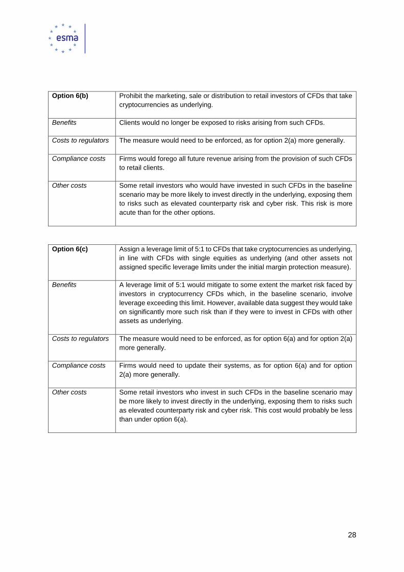
Option 6(b) Prohibit the marketing, sale or distribution to retail investors of CFDs that take
cryptocurrencies as underlying.
Benefits Clients would no longer be exposed to risks arising from such CFDs.
Costs to regulators The measure would need to be enforced, as for option 2(a) more generally.
Compliance costs Firms would forego all future revenue arising from the provision of such CFDs
to retail clients.
Other costs Some retail investors who would have invested in such CFDs in the baseline
scenario may be more likely to invest directly in the underlying, exposing them
to risks such as elevated counterparty risk and cyber risk. This risk is more
acute than for the other options.
Option 6(c) Assign a leverage limit of 5:1 to CFDs that take cryptocurrencies as underlying,
in line with CFDs with single equities as underlying (and other assets not
assigned specific leverage limits under the initial margin protection measure).
Benefits A leverage limit of 5:1 would mitigate to some extent the market risk faced by
investors in cryptocurrency CFDs which, in the baseline scenario, involve
leverage exceeding this limit. However, available data suggest they would take
on significantly more such risk than if they were to invest in CFDs with other
assets as underlying.
Costs to regulators The measure would need to be enforced, as for option 6(a) and for option 2(a)
more generally.
Compliance costs Firms would need to update their systems, as for option 6(a) and for option
2(a) more generally.
Other costs Some retail investors who invest in such CFDs in the baseline scenario may
be more likely to invest directly in the underlying, exposing them to risks such
as elevated counterparty risk and cyber risk. This cost would probably be less
than under option 6(a).

29
3 Simulation results informing leverage limits
27. ESMA has undertaken a quantitative simulation of the distribution of returns an investor might
expect to receive at different leverage levels. The model takes as its starting point several years
of market price data for various assets that are commonly used as underlying in CFD contracts
sold to retail customers. Using these data, ESMA has simulated returns that investors in CFDs
using these reference assets would have received for a range of values of initial leverage.
28. The simulation exercise focuses on the probability of margin close-out (MCO) as a measure of
investor detriment. Specifically, the results quantify the probability of MCO assuming a single
CFD position that is automatically closed out at precisely 50% of minimum required initial
margin whenever the margin on the position reaches this level.
29. Setting leverage limits based on individual positions is appropriate for two main reasons. First,
responses to the call for evidence and data from NCAs indicate that a significant share of
investors hold only a single position in their account, and leverage limits are designed to
improve outcomes and reduce risk for retail investors including this population. Second,
analysis using market price time series for individual assets is a tractable way to model risk,
reflected in the fact that firms themselves use such an analytical framework to inform their risk
management.17 Modelling portfolios for the purpose of this simulation, in contrast, could not be
representative of a significant number of investor positions due to the very large number of
positions that can be included in a portfolio.
30. As set out in the Decision, a number of other issues in the market for retail CFDs pose a
potential or actual source of consumer detriment. These include, but are not limited to, the
complexity of the product, lack of transparency in its provision, the potential for conflicts of
interest to arise and issues in relation to marketing and distribution. These topics are outside
the scope of the simulation exercise, which was undertaken to inform the setting of leverage
limits.
31. The rest of this section of the document:
explains how the model works;
discusses the assumptions made and the reasons for choosing to study certain metrics; and
discusses the sensitivity of the model to changes in the assumptions.
32. Results by individual underlying asset are listed in Annex I. A more detailed description of the
methodology is provided in Annex II. Finally, Annex III discusses in detail the data and evidence
used to inform the assumptions and focus of the simulation exercise.
17 For instance, analysis provided to ESMA by the UK CFD Association in response to the call for evidence, and which was carried
out on behalf of the Association by CMC Markets, modelled the Conditional Variance at Risk (CVaR) of individual assets on a
broadly similar basis to the ESMA model described herein, though the focus on CVaR differs from the ESMA approach. The CMC
Markets analysis used a 15 year time series of close-to-open market price movements and reported 95% CVaR values. According
to their results, close-to-open price movements tend to show lower price variation than that displayed by the intra-day open-to-
low movements taken into account in the ESMA simulation. The ordinal ranking of CVaR values for major and minor indices
accords closely with the categorisation proposed by ESMA in the call for evidence. The one difference in this respect between
ESMA’s proposal and the reported ranking, and highlighted by CMC Markets, was the ordinal ranking of the EuroSTOXX50.
Following further analysis, ESMA has reassigned the EuroSTOXX50 to the asset class of major indices. The NASDAQ 100 index
has also been included in the asset class of major indices, reflecting its prominent use by major firms and the fact the relevant
simulation results are close to those of the NASDAQ Composite index, a comparable index classed as major in this context.

30
3.1 Methodology
33. ESMA has undertaken a quantitative simulation of the distribution of returns an investor might
expect to receive at different leverage levels. The model takes as its starting point several years
of daily market price data for various assets that are commonly used as reference assets in
CFDs sold to retail customers.
34. These data can be used to simulate returns that investors in CFDs using these reference assets
would have received over a given period, for different leverage levels. For example, the
simulation of a position held for one day with a given asset as underlying involves taking an
average of the return imputed for each day for which there is data in the time series of market
prices for that asset.18
35. The average return calculation takes into account a 50% MCO rule, the operation of which
depends on the initial margin requirement. The model does this by comparing the intra-day low
price of the asset in question with the market open price. For instance, assuming a leverage
level of 40:1, i.e. initial investor margin of 2.5%, then if the intra-day low price is 1.25% below
the market open price or lower, the position is taken to be closed out, and a return of -1.25%
(expressed as a percentage of total exposure) is imputed for that day. If the intra-day low price
represents a fall of less than 1.25% in magnitude compared to the market open price, then the
position is taken to remain open until the end of the day, with that day’s return calculated as the
change from market open to market close, expressed as a percentage of the former.
36. Following this procedure, the model compares how likely MCO is to happen at different
leverage levels. This is on the assumption that MCO is automatic and perfectly executed (e.g.
slippage with the close-out is not considered). The model calculates the probability of close-out
as a function of leverage. Based on this, the model determines the leverage level that implies
a 5% probability of MCO.19 This will be referred to as the ‘MCO metric’.20
37. The results cover durations of 1, 2, 3, 4 and 5 days. For periods of longer than one day, the
model takes into account the intra-day lows for each day in the period when determining
whether a position is closed out. An additional feature of the model is that, for realism, it takes
into account overnight financing costs. However, as the sensitivity analysis of section 3.4
shows, the impact of costs, spreads and charges on the MCO metric is generally relatively
minor.21
3.1.1 Alternative approaches
38. The simulation exercise, based on lengthy time series of market price data, is not the only
possible approach ESMA could have taken. For instance, the Netherlands Authority for
18 The model assumes long positions throughout. Section 3.4 provides an example robustness check to show that short positions yield similar results to long positions, a result that would be expected from a theoretical perspective for the reason of approximate symmetry in short-run movements in asset prices.
19 In section 3.4, this 5% reference probability is varied as part of the sensitivity analysis of the model.
20 Assessing the probability of MCO as a function of leverage is not the only possible metric that could be relevant to assessing consumer detriment. The simulation exercise also allows for calculations of other statistics relating to distributions of investor returns. For example, the expectation of the return for different leverage levels can be computed. Such additional statistics were used in “sense-checking” the model, but were not the primary focus of the exercise.
21 The sensitivity analysis presented in Chart 8 in section 3.3 examines the impact of varying the spreads modelled. The impact of overnight financing charges, for the time periods studied, is smaller still.

31
Financial Markets (AFM), in a previously published report on leveraged products, simulated
investor returns based on theoretical return distributions.22 This approach would remove the
need to rely on data, in turn improving the flexibility of the model and making it easier to test its
robustness. It would not, on the other hand, reduce reliance on the parameter assumptions.
Also, the choice of theoretical return distribution could be complicated by the fact that in addition
to assuming a distribution of returns of the underlying for a given holding period, another
variable of interest is the lowest price of the underlying during the holding period, which would
need to be assumed in a theoretical model. This could be achieved by, for example, assuming
a biased random walk process as in the Black-Scholes-Merton model. However, this would
clearly be a complicating factor, and the particular theoretical return distribution assumptions
would need substantive justification.
3.2 Assumptions and focus of simulation exercise
3.2.1 Assumptions
39. The simulation exercise makes the following key assumptions:
Assumption 1: Costs. Investors naturally face transaction costs when opening (and in some
cases, when closing) a position. The model allows for spreads, commissions (i.e.
percentage changes on total exposure) and overnight financing fees. These costs are
mostly based on public information provided by the largest provider in the market, IG Group
a UK-based firm.23 24 ESMA also used this provider’s website to help identify a relevant set
of assets to use in the model, in some cases additionally using the websites of two other
large providers.25
Data on fees and charges gathered from several providers’ websites suggest that the
largest providers offer relatively low fees (plausibly due to economies of scale). Sensitivity
analysis suggests that the model’s results – specifically the MCO metric – generally have
low sensitivity to the cost parameter within the range of observed fees, so the exact choice
has limited impact on intervention considerations.26 The sensitivity analysis compares zero
costs with a “high” cost assumption of three times the core cost assumption.27
22 See AFM (2013), ‘Rapport hefboomproducten – Resultaten onderzoek’ (in Dutch).
23 The company website is http://www.ig.com. This simple approach makes it easy to verify that the costs are correctly imputed. In some cases, especially commodities contracts, the existence of different contract sizes in the market can complicate this task.
24 An exception was in respect of cryptocurrencies, for which a 1% commission assumption was used as a proxy for the spread quoted by IG Group. The reason for applying a percentage commission rather than an absolute spread was that the price level of cryptocurrencies changed by orders of magnitude during the time series.
25 Spreads were checked for outliers against those offered by CMC Markets and Plus500 Ltd, whose respective websites are https://www.cmcmarkets.com/en/ and https://www.plus500.com/. These websites were also used in selecting pairs of minor currencies to model in the simulation exercise, as described in Annex III.
26 In other words, the MCO metric as applied to the data and parameters used in the model generally yields leverage values that ensure that typical investment costs do not deplete margin sufficiently to strongly affect the MCO probability. The leverage limits thereby mitigate the problem that high leverage leads to per trade costs that deplete much or all of an investor’s margin. Leverage is also associated with higher volumes of trading by investors, increasing trading costs via repeated entering and exiting of positions. The leverage limits are also expected to address this issue, as noted in the discussion of the relevant intervention options in section 2.
27 To help inform the “high cost” variant, for insight into the variation of costs in the market, ESMA examined the websites of 16 providers.
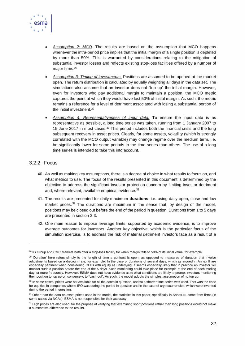
32
Assumption 2: MCO. The results are based on the assumption that MCO happens
whenever the intra-period price implies that the initial margin of a single position is depleted
by more than 50%. This is warranted by considerations relating to the mitigation of
substantial investor losses and reflects existing stop-loss facilities offered by a number of
major firms.28
Assumption 3: Timing of investments. Positions are assumed to be opened at the market
open. The return distribution is calculated by equally weighting all days in the data set. The
simulations also assume that an investor does not “top up” the initial margin. However,
even for investors who pay additional margin to maintain a position, the MCO metric
captures the point at which they would have lost 50% of initial margin. As such, the metric
remains a reference for a level of detriment associated with losing a substantial portion of
the initial investment.29
Assumption 4: Representativeness of input data. To ensure the input data is as
representative as possible, a long time series was taken, running from 1 January 2007 to
15 June 2017 in most cases.30 This period includes both the financial crisis and the long
subsequent recovery in asset prices. Clearly, for some assets, volatility (which is strongly
correlated with the MCO output variable) may change regime over the medium term, i.e.
be significantly lower for some periods in the time series than others. The use of a long
time series is intended to take this into account.
3.2.2 Focus
40. As well as making key assumptions, there is a degree of choice in what results to focus on, and
what metrics to use. The focus of the results presented in this document is determined by the
objective to address the significant investor protection concern by limiting investor detriment
and, where relevant, available empirical evidence.31
41. The results are presented for daily maximum durations, i.e. using daily open, close and low
market prices.32 The durations are maximum in the sense that, by design of the model,
positions may be closed out before the end of the period in question. Durations from 1 to 5 days
are presented in section 3.3.
42. One main reason to impose leverage limits, supported by academic evidence, is to improve
average outcomes for investors. Another key objective, which is the particular focus of the
simulation exercise, is to address the risk of material detriment investors face as a result of a
28 IG Group and CMC Markets both offer a stop-loss facility for when margin falls to 50% of its initial value, for example.
29 ‘Duration’ here refers simply to the length of time a contract is open, as opposed to measures of duration that involve adjustments based on a discount rate, for example. In the case of durations of several days, which as argued in Annex II are especially pertinent when considering CFDs with equity as underlying, it seems especially likely that in practice an investor will monitor such a position before the end of the 5 days. Such monitoring could take place for example at the end of each trading day, or more frequently. However, ESMA does not have evidence as to what conditions are likely to prompt investors monitoring their position to top up or, conversely, to “cash out”. As such, the model adopts the simplest assumption of no top up.
30 In some cases, prices were not available for all the dates in question, and so a shorter time series was used. This was the case for equities in companies whose IPO was during the period in question and in the case of cryptocurrencies, which were invented during the period in question.
31 Other than the data on asset prices used in the model, the statistics in this paper, specifically in Annex III, come from firms (in some cases via NCAs). ESMA is not responsible for their accuracy.
32 High prices are also used, for the purpose of verifying that examining short positions rather than long positions would not make a substantive difference to the results.

33
single position moving adversely. Leverage limits are also expected to ameliorate the size and
speed of loss for each trade prior to the position being automatically closed out by the firm.33
43. An overriding concern in this context is to mitigate the risk of substantial investor detriment from
trading in CFDs. For very short-run speculative trades (e.g. those of less than an hour), the
scope for many repeated trades and resulting transaction costs mean that cumulative losses
are likely to be significant. In the case of longer term trades – for instance, investors holding
positions for a day or more – an important source of the risk of detriment is from being
automatically closed out due to adverse movements in the price of the underlying. The leverage
limits are calibrated to address this second source of risk. However, lower leverage is also
expected to improve outcomes for investors by reducing trading volumes, reducing the size and
impact of loss-making positions, and reducing the relative impact of transaction fees as a
proportion of the client’s initial and ongoing investment. Academic evidence demonstrates that
leverage limits materially improve outcomes for consumers on a per trade basis as well as
overall (i.e. per investor account).
44. The data from firms presented in Annex III confirm that many trades are of extremely short
durations, for instance of less than one hour. Investors making these trades, who may be “day
traders” aiming to time the market, are far less likely to be closed out than investors making
longer trades in the order of a day or more.34 However, the data in Annex III also show that a
significant number of trades, across all asset classes and according to all available data
sources, are undertaken for a day or more. This suggests that from an intervention perspective,
high leverage has a significant detrimental effect on a significant number of investors who trade
for a day or more.
45. The available data show consistently that trades in equities are typically of longer duration than
other trades. From an intervention perspective, as regards equity CFDs in particular, this
warrants giving consideration to the upper end of the durations presented in the results of
section 3.3.35
46. Another degree of freedom in presenting the results of the model is in choosing a reference
probability of 5%, i.e. calculating what leverage implies that MCO occurs with a probability of
5%.36 This choice of focus, taken together with the focus on durations and the MCO assumption
itself, is taken to be a measure of a significant risk of investor detriment. The results are
sensitive in this respect, as set out in section 3.4.
47. Finally, the selection of assets was a significant and necessary choice with regard to the
scope and focus of the modelling. In general, assets were chosen based on proxies for volumes
traded by retail investors, as detailed in Annex III. For example, the major currency pairs
modelled are all those pairs in which both assets are among the 6 most frequently traded on
global markets.37 In some cases, data consideration of market volumes together with market
33 Theoretical analysis of leverage limits by IG Group, provided in the call for evidence, focuses on the win versus loss probability of a single trade. The analysis suggests that very high leverage significantly reduces the per-trade win probability.
34 Such investors face other issues, such as the fact they will cross the spread many times in making trades.
35 However, the data are extremely heterogeneous, preventing the identification of an exact rule by which this should be done
36 More precisely, the results identify the maximum integer leverage value that implies an MCO probability that does not strictly exceed 5%.
37 Based on commercially available market-wide data for October 2017 provided by an NCA. 15 pairs are therefore modelled to cover those pairs in which both currency is one of the majors, i.e. the 6 most traded globally, as reflected in the definition adopted. This total excludes the reverse of a given pair, e.g. only counting EUR/USD rather than also USD/EUR. According to the data, the 7th most-traded pair is AUD, which was tested but implied leverage limits in line with minor currencies. Several AUD pairs (as listed in Table A.3 in Annex I) are modelled among minor currencies, for the sake of representativeness and in accordance with the sample selection procedure listed in Annex III.

34
intelligence prompts focus on particular assets from an intervention perspective, e.g. gold and
oil in the case of commodities. Such assets are highlighted in the graphical results that follow.
3.3 Results
48. Charts 1 to 7 below show the corridor of leverage needed, across a given asset class, for a 5%
probability of MCO to take place, given a maximum position duration ranging from 1 day to 5
days. For illustrative purposes, the charts also include the limits imposed by the intervention
measures. The main results from the model, in terms of the MCO metric, are presented below.
Chart 7, which presents results from cryptocurrencies, is by necessity based on less data than
the other charts, as shorter time series are available for these relatively immature assets. The
immaturity of the market means that previous price variability may not be a reliable guide to
future variability. In interpreting Chart 7, in addition to noting these limitations, it is also
particularly important to note that only market risk is taken into account in the simulation
exercise. The impact analysis in section 2 describes some other sources of risk faced by
investors in this context.
Chart 1: Leverage limits that imply 5% simulated probability of MCO, by holding period, with commodities
as underlying
49. In Chart 1, the shaded area shows the range between the commodity modelled with the lowest
leverage implying a 5% probability of MCO and the commodity with the highest leverage
implying a 5% probability of MCO, across different holding periods measured in days.
50. As mentioned above, among commodities, evidence (from data on commodities trading
volumes on exchange, as a proxy, together with market intelligence from NCAs) indices that
two assets are by far the most frequently traded by retail investors. These assets – namely gold
0
5
10
15
20
25
30
1 2 3 4 5Levera
ge i
mpliyin
g 5
% M
CO
pro
babilit
y
Maximum days position open
Lowest asset value Highest asset value
Gold Oil
Leverage limit (non-gold commodities) Leverage limit (gold)
Note: Simulated leverage levels that imply a 5% probability of margin close out (MCO) in the model, where MCO is set to 50%, plotted alongsideleverage limits being introduced of 20:1 leverage for gold and 10:1 leverage for other commodities, for different maximum durations in the model, i.e.the length of time a position is left open if it is not closed out. "Highest asset value"=maximum leverage among all assets in sample (n=15) tested
implying a simulated 5% probability of MCO. "Lowest asset value" is minimum such leverage. "Oil"= leverage limit for Brent crude oil that implies asimulated 5% probability of MCO. "Gold"=leverage limit for gold that implies a simulated 5% probability of MCO.Sources: Thomson Reuters, ESMA.

35
and oil – are indicated separately in Chart 1.38 The implied leverage limits for oil based on the
simulation are at the lower end of the range, with the lowest in general being natural gas, as
can be seen from the results for individual assets tabulated in Annex I. Market price data on
natural gas unsurprisingly therefore exhibit similar characteristics as those for oil relevant to the
present context.39
51. Charts 2 to 7 present analogous results for the other types of assets set out in the intervention
measure.
Chart 2: Leverage limits that imply 5% simulated probability of MCO, by holding period, with pairs of
major currencies as underlying
38 The oil benchmark highlighted in Chart 1 is Brent crude. Another widely-used benchmark is West Texas Intermediate, the results for which are broadly similar, are included in the range of values (grey shaded area) in Chart 1 and are reported separately in Table A1 in Annex I.
39 NCA market intelligence suggests that natural gas CFDs are popular with retail investors. Commercially available market-wide data provided by an NCA on exchange-traded volumes of standard commodities contracts for the first 9 months of 2017 showed that around USD 48bn of Brent oil futures were traded and around USD 35bn for gold. Third was gasoline, at around USD 14bn and fourth was natural gas, at USD 13bn. Results for all these assets are presented in Table A1 in Annex I.
0
10
20
30
40
50
60
1 2 3 4 5
Leve
rage im
pliy
ing 5
% M
CO
pro
babili
ty
Maximum days position open
Lowest asset value Highest asset value Leverage limit
Note: Simulated leverage levels that imply a 5% probability of margin close out (MCO) in the model, where MCO is set to 50%, plotted alongsideleverage limit being introduced of 30:1 for pairs of major currencies, as defined in Decision, for different maximum durations in the model, i.e. thelength of time a position is le ft open if it is not closed out. "Highest asset value"=maximum simulated leverage among all assets in question excluding
reverses of given pairs (n=15) implying a simulated 5% probability of MCO. "Lowest asset value" is minimum such leverage.Sources: Thomson Reuters, ESMA.

36
Chart 3: Leverage limits that imply 5% simulated probability of MCO, by holding period, with pairs of
currencies that include at least one non-major currency taken as underlying
Chart 4: Leverage limits that imply 5% simulated probability of MCO, by holding period, with major equity
indices as underlying
0
5
10
15
20
25
30
35
40
45
50
1 2 3 4 5Levera
ge im
pliy
ing 5
% M
CO
pro
babili
ty
Maximum days position open
Lowest asset value Highest asset value Leverage limit
Note: Simulated leverage levels that imply a 5% probability of margin close out (MCO) in the model, where MCO is set to 50%, plotted alongsideleverage limit being introduced of 20:1 for currency pairs involving mon-major currencies, as defined in the Decision, for different maximumdurations in the model, i.e . the length of time a position is left open if it is not closed out. "Highest asset value"=maximum simulated leverage among
all assets in sample (n=18) implying a simulated 5% probability of MCO. "Lowest assetvalue" is minimum such leverage.Sources: Thomson Reuters, ESMA.
0
5
10
15
20
25
30
1 2 3 4 5
Levera
ge im
pliy
ing 5
% M
CO
pro
babili
ty
Maximum days position open
Lowest asset value Highest asset value Leverage limit
Note: Simulated leverage levels that imply a 5% probability of margin close out (MCO) in the model, where MCO is set to 50%, plotted alongsideleverage limit being introduced of 20:1 for major equity indices, as defined in the Decision, for different maximum durations in the model, i.e. the length oftime a position is left open if it is not closed out. "Highest asset value"=maximum simulated leverage among all assets in question (n=10) implying a
simulated 5% probability of MCO. "Lowest assetvalue" is minimum such leverage.Sources: Thomson Reuters, FCA, ESMA.
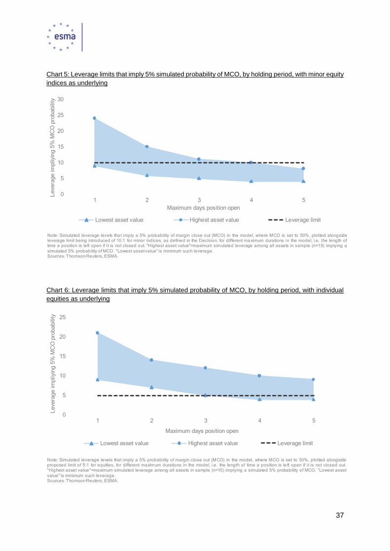
37
Chart 5: Leverage limits that imply 5% simulated probability of MCO, by holding period, with minor equity
indices as underlying
Chart 6: Leverage limits that imply 5% simulated probability of MCO, by holding period, with individual
equities as underlying
0
5
10
15
20
25
30
1 2 3 4 5
Levera
ge im
pliy
ing 5
% M
CO
pro
babili
ty
Maximum days position open
Lowest asset value Highest asset value Leverage limit
Note: Simulated leverage levels tha t imply a 5% probability of margin close out (MCO) in the model, where MCO is set to 50%, plotted alongsideleverage limit being introduced of 10:1 for minor indices, as defined in the Decision, for different ma ximum durations in the model, i.e. the length oftime a position is left open if it is not closed out. "Highest asset value"=maximum simulated leverage among all assets in sample (n=19) implying a
simulated 5% probability of MCO. "Lowest assetvalue" is minimum such leverage.Sources: Thomson Reuters, ESMA.
0
5
10
15
20
25
1 2 3 4 5
Leve
rage im
pliy
ing 5
% M
CO
pro
babili
ty
Maximum days position open
Lowest asset value Highest asset value Leverage limit
Note: Simulated leverage levels that imply a 5% probability of margin close out (MCO) in the model, where MCO is set to 50%, plotted alongsideproposed limit of 5:1 for equities, for different maximum durations in the model, i.e. the length of time a position is le ft open if it is not closed out."Highest asset value"=maximum simulated leverage among all assets in sample (n=15) implying a simulated 5% probability of MCO. "Lowest asset
value" is minimum such leverage.Sources: Thomson Reuters, ESMA.

38
52. Chart 6, which covers equities, takes as a core sample the largest 6 US companies as, the
largest 6 based in Europe and the largest 3 from the rest of the world. More details are provided
in Annex III.
53. In interpreting Chart 6, it is important to note that equity CFDs are in general held for much the
longest among different asset classes. For this reason, in setting leverage limits for CFDs with
individual equities as underlying, ESMA took into account especially the upper end of the
durations presented.
Chart 7: Leverage limits that imply 5% simulated probability of MCO, by holding period, with
cryptocurrencies as underlying
54. As highlighted above, Chart 7 is based on less data than the other charts because the assets
are relatively new. The immaturity of the market means that previous price variability may not
be a reliable guide to future variability in assessing market risk, and the impact analysis in
section 2 describes some other sources of risk faced by investors in this context.
55. The results for individual cryptocurrencies plotted in Chart 7 illustrate some of the limitations in
making inferences based on the available data. The results for Bitcoin are based on a longer
time series – nearly 4 years – than for the other assets, for which less than a year of data is
available. As a result, developments in the cryptocurrency market in 2017 are less of a driver
for the results in respect of Bitcoin than the results for the other cryptocurrencies modelled.
3.4 Sensitivity analysis
56. To assist in the interpretation of the results in section 3.3, ESMA analysed the sensitivity of the
model to changes in its parameters. In particular, Charts 8 to 10 compare variations in the cost
assumption, the MCO assumption (i.e. varying the percentage of initial margin that triggers
MCO) and finally the reference probability used (cf. the focus in section 3.3 on a 5% probability
of MCO). For illustration, results are provided for the sample of minor equity indices modelled
0
1
2
3
4
5
1 2 3 4 5
Levera
ge im
pliy
ing 5
% M
CO
pro
babili
ty
Maximum days position open
Bitcoin Ether Ripple Leverage limit
Note: Simulated maximum leverage levels that imply a 5% probability of margin close out (MCO) in the model, where MCO is set to 50%, plottedalongside leverage limit being introduced of 2:1 for cryptocurrencies for different maximum dura tions in the model, i.e. the length of time a position is leftopen if it is not automatically closed out. Simulated results for Litecoin also included in range, but not plotted separately in this chart.
Sources: FCA, ESMA.
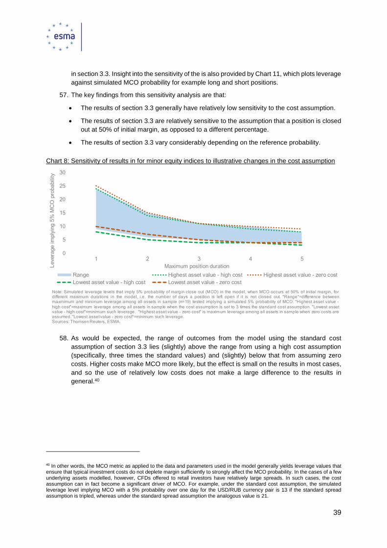
39
in section 3.3. Insight into the sensitivity of the is also provided by Chart 11, which plots leverage
against simulated MCO probability for example long and short positions.
57. The key findings from this sensitivity analysis are that:
The results of section 3.3 generally have relatively low sensitivity to the cost assumption.
The results of section 3.3 are relatively sensitive to the assumption that a position is closed
out at 50% of initial margin, as opposed to a different percentage.
The results of section 3.3 vary considerably depending on the reference probability.
Chart 8: Sensitivity of results in for minor equity indices to illustrative changes in the cost assumption
58. As would be expected, the range of outcomes from the model using the standard cost
assumption of section 3.3 lies (slightly) above the range from using a high cost assumption
(specifically, three times the standard values) and (slightly) below that from assuming zero
costs. Higher costs make MCO more likely, but the effect is small on the results in most cases,
and so the use of relatively low costs does not make a large difference to the results in
general.40
40 In other words, the MCO metric as applied to the data and parameters used in the model generally yields leverage values that ensure that typical investment costs do not deplete margin sufficiently to strongly affect the MCO probability. In the cases of a few underlying assets modelled, however, CFDs offered to retail investors have relatively large spreads. In such cases, the cost assumption can in fact become a significant driver of MCO. For example, under the standard cost assumption, the simulated leverage level implying MCO with a 5% probability over one day for the USD/RUB currency pair is 13 if the standard spread assumption is tripled, whereas under the standard spread assumption the analogous value is 21.
0
5
10
15
20
25
30
1 2 3 4 5
Levera
ge i
mply
ing 5
% M
CO
pro
babilit
y
Maximum position duration
Range Highest asset value - high cost Highest asset value - zero cost
Lowest asset value - high cost Lowest asset value - zero cost
Note: Simulated leverage levels that imply 5% probability of margin close out (MCO) in the model, when MCO occurs at 50% of initial margin, fordifferent maximum durations in the model, i.e. the number of days a position is left open if it is not closed out. "Range"=difference betweenmaxmimum and minimum leverage among all assets in sample (n=19) tested implying a simulated 5% probability of MCO. "Highest asset value -
high cost"=maximum leverage among all assets in sample when the cost assumption is set to 3 times the standard cost assumption. "Lowest assetvalue - high cost"=minimum such leverage. "Highest asset value - zero cost" is maximum leverage among all assets in sample when zero costs areassumed."Lowest assetvalue - zero cost"=minimum such leverage.Sources: Thomson Reuters, ESMA.

40
Chart 9: Sensitivity of results in for minor equity indices to illustrative changes in the MCO assumption
Chart 10: Sensitivity of results in for minor equity indices to illustrative changes in the reference
probability
0
5
10
15
20
25
30
35
40
1 2 3 4 5Le
ve
rag
e im
pliy
ing
5%
MC
O p
robability
Maximum position duration
Range - 50% MCO Highest asset value - 30% MCO Lowest asset value - 30% MCO
Highest asset value - 70% MCO Lowest asset value - 70% MCO
Note: Simulated leverage levels tha t imply 5% probability of margin close out (MCO) in the model, when MCO is assumed to occur at selected values,for different maximum durations in the model, i.e. the number of days a position is left open if it is not closed out. "Range"=difference betweenmaxmimum and minimum leverage among all assets in sample (n=19) implying a simulated 5% probability of MCO. "Highest asset value - 70%
MCO"=maximum leverage among all assets in sample implying a simulated 5% probability of MCO, when MCO is set to 70%. "Lowest asset value -70% MCO"=minimum such leverage. "Highest asset value - 30% MCO"=maximum leverage among all assets in sample implying a simulated 5%probability of MCO when MCO is set to 30%. "Lowest assetvalue - 30% MCO"=minimum such leverage.Sources: Thomson Reuters, ESMA.
0
5
10
15
20
25
30
35
1 2 3 4 5
Levera
ge im
pliy
ing g
iven p
robabili
ty o
f M
CO
Maximum duration position open
Range 10% reference probability - highest asset
10% reference probability - lowest asset 2% reference probability - highest asset
2% reference probability - lowest asset
Note: Simulated leverage levels that imply given probability of margin close out (MCO) in the model, when MCO occurs at 50% of initial margin fordifferent maximum durations in the model, i.e . the number of days a position is left open if it is not closed out. "Range"=difference between maximumand minimum leverage among all assets in sample (n=19) implying a simulated 5% probability of MCO. "2% reference probability - highest
asset"=maximum leverage among all assets in sample implying MCO with 2% probability. "2% reference probability - lowest asset"=minimum suchleverage. "10% reference probability - highest asset"=maximum leverage among all assets in sample implying MCO with 10% probability. "10%reference probability - lowest asset"=minimum such leverage.Sources: Thomson Reuters, ESMA.

41
Chart 11: Comparison of results for simulated long and short positions in example equity indices
59. Chart 11 uses a different approach to graphing the relationship between leverage and MCO
probability than do Charts 1-10. The horizontal axis represents leverage level, and the vertical
axis MCO probability, under the standard assumption of MCO at 50% for a single position. Two
points are of note. The first is that there is generally a small difference between the long and
short positions simulated, though the size of this difference varies without any discernible
pattern as leverage increases. This reflects the fact the data-based simulation exploits actual
price movements in the presumed underlying rather than simply comparing theoretical
distributions. The fact the difference in results between the long and short positions is small
suggests the focus on long-only positions throughout Charts 1-10 is appropriately
representative. The second point is that plotting the relationship between leverage and MCO
probability shows a fairly steep increase in the latter as the former rises over the range of
leverages on the horizontal axis. This provides insight into the sensitivity of the previous results
to the assumption of MCO at 50% of initial margin. A given change in the reference probability
(represented on the vertical axis) will lead to a larger change in the required leverage the
steeper the curve is at the relevant values.
0%
10%
20%
30%
40%
50%
60%
1 5 10 15 20 25 30 35 40 45 50 55 60 65 70 75 80 85 90 95 100
S&P500 long DAX30 long S&P500 short DAX30 short
Note: Simulated close out probability by leverage for selected major indices, assuming a 50% MCO rule. "DAX30 long" simulates a long position in a CFD with the DAX30 index asunderlying. "DAX 30 short" simula tes a short position in a CFD with the DAX30 index as underlying. "S&P 500 long" simulates a long position in a CFD with the Standard & Poor's 500index as underlying. "S&P500 short" simulates a short position in a CFD with the Standard & Poor's 500 index as underlying.
Sources: Thomson Reuters, ESMA.

42
4 Annexes
Annex I – Core results for individual assets

43

44

45

46

47

48

49
Annex II – Detailed methodology
4.1.1 Raw data
60. The model takes as its primary input commercially-available market price data for different
reference assets. In most cases, daily price data is taken covering over 10 years, from January
2007 to June 2017. Notable exceptions were cryptocurrencies, where data are only available
for more recent years, reflecting that these assets are recent innovations. 41 For example, one
time series used is the daily open price for the DAX30 index over this period, comprising 2,655
observations. In all cases, the raw data used throughout (i.e. for open, close, high and low
prices) are the prices at which respectively the first, last, highest-price and lowest-price trade
took place, which means that the raw data include no spread.42 These transaction prices will
be referred to as the “raw open price”, “raw close price”, and so on.
4.1.2 Adjusting the raw data for the purpose of simulating returns
61. Based on the data, the model simulates the expected distribution of returns for an investor who
opens their position on a randomly selected day, if all days in the sample are equally likely to
be chosen.43 The simulated returns for each period in the time series give a distribution from
which summary statistics such as the expected return can be calculated.
62. This section explains how a single return is simulated for an arbitrary starting point in the time
series, which is open for some number 𝑡 = 1,2, … of days.
63. Neglecting for the moment the effect of fees and charges, the gross return to an investor from
a long position in a CFD expressed as a percentage of total exposure is the percentage
difference between the price of a reference asset when the position was opened and the price
of that asset when the position was closed. The model calculates gross returns in the case of
a 5-day position by subtracting the close price on day 5 from that on day 1 and dividing by the
open price on day 1. (In other words, calculations are done for all available rolling 5-day
increments.) This gives a percentage change in the price over the period in question.
64. Rather than simply calculating gross returns, however, the simulated returns are adjusted by
assumed fees, spreads and charges, based on public information from the largest provider in
the retail market for CFDs, IG Group.44 In general, the key source of revenue for firms from
investors is through bid-ask spreads. A feature of the model throughout is that fees and spreads
41 Fewer observations are available for certain other assets. This depends partly on the fact different assets may have different trading periods and trading days, but more significantly in certain cases (e.g. Facebook shares) because the underlying was only created more recently than 2007.
42 Using trade price data throughout thus allows the provider spread to be modelled by making simple adjustments to the open price, as described below.
43 The observations therefore overlap one another in this case. For example, the DAX30 data is used to calculate a simulated return over 5 consecutive trading days starting on the first day in the time series, then another simulated return over 5 consecutive trading days starting on the second day in the time series, and so on. Simple statistical inference of this kind – as opposed to inference of say confidence intervals – does not require any adjustment for the data overlap.
44 Spreads were checked for outliers against public information on spreads offered by two other large providers, CMC Markets and Plus500.

50
are incorporated in the calculation of gross returns by adjusting the prices investors face.45 For
example, to take account of the spread that providers include on CFDs in the EUR/USD
currency pair, the raw open price on day 1 is increased by 0.75 pips. The result is the adjusted
open price, denoted 𝑝𝑜𝑝𝑒𝑛, defined as follows.
𝑝𝑜𝑝𝑒𝑛 ≡ (𝑟𝑎𝑤 𝑜𝑝𝑒𝑛 𝑝𝑟𝑖𝑐𝑒 𝑜𝑛 𝑑𝑎𝑦 1) + 𝑠𝑝𝑟𝑒𝑎𝑑 (1)
65. Raw intra-period low and raw close prices do not need to be adjusted to take account of the
spread, as the difference between a raw close price and an adjusted open price, for example,
incorporates the spread. Likewise, if a commission is charged by the provider (which is the
case for some CFDs in individual equities, for example), the raw open price is revised upwards.
However, the raw intra-period low prices and raw close prices are adjusted to take account of
overnight financing charges.46 In the case of a 5-day position, for example, the adjusted close
price on day t, denoted 𝑝𝑡𝑐𝑙𝑜𝑠𝑒, involves subtracting the overnight financing fee multiplied by 4
(since there are 4 overnight periods) from the raw close price. It is defined as follows, for a
position of some number 𝑡 = 1,2, … of days.
𝑝𝑡𝑐𝑙𝑜𝑠𝑒 ≡ (𝑟𝑎𝑤 𝑐𝑙𝑜𝑠𝑒 𝑝𝑟𝑖𝑐𝑒 𝑜𝑛 𝑑𝑎𝑦 𝑡) − (𝑜𝑣𝑒𝑟𝑛𝑖𝑔ℎ𝑡 𝑓𝑖𝑛𝑎𝑛𝑐𝑖𝑛𝑔 𝑓𝑒𝑒) × (𝑡 − 1) (2)
66. Likewise, the adjusted low price on day t , denoted 𝑝𝑡𝑙𝑜𝑤, is defined as follows
𝑝𝑡𝑙𝑜𝑤 ≡ (𝑟𝑎𝑤 𝑙𝑜𝑤 𝑝𝑟𝑖𝑐𝑒 𝑜𝑛 𝑑𝑎𝑦 𝑡) − (𝑜𝑣𝑒𝑟𝑛𝑖𝑔ℎ𝑡 𝑓𝑖𝑛𝑎𝑛𝑐𝑖𝑛𝑔 𝑓𝑒𝑒) × (𝑡 − 1) (3)
4.1.3 MCO assumption
67. In some cases in the model, depending on price movements, the position is assumed to be
closed out. To specify an MCO assumption, first define two variables. The first of these is the
(initial) leverage of a position, denoted 𝐿.47 𝐿 is the ratio of total exposure to the initial margin
posted. For example, if 𝐿 = 1 (i.e. the position is unleveraged) then a 3% return on a €100,000
investment is €3,000. A higher value of leverage 𝐿 will multiply any returns/losses; if 𝐿 = 20,
then a 3% return on a €100,000 investment becomes €3,000 × 20 = €60,000.
68. Looking at things from another perspective, if an investor posts initial margin of €100, for
example, and the notional value of the CFD is €2,500, then 𝐿 = 25. Consequently, if the price
of the reference asset rises by 3%, the gross return on the position is (3% × €100) × 25 = €75.
Alternatively expressed, this is a 75% return on initial margin. The initial margin expressed as
a percentage of total exposure is therefore given by 1
𝐿.48 If 𝐿 = 25, then the initial margin is 4%
of total exposure.
45 This is equivalent to assuming investors do not pay fees as such but face prices that give them an equivalent return to that which they would receive if they did pay fees.
46 Financing charges are the one feature of the model that is not symmetric with respect to long versus short positions; in practice, an investor’s short position may in fact be credited with a very small amount in relation to overnight financing. However, over the holding periods modelled, financing-related payments have a very small impact on results. In the case of long positions in assets other than cryptocurrencies, a typical overnight financing charge is 2.5% (annualised) + base rate, but as the effect of the base rate is negligible, the 2.5% annualised figure was simply used for simplicity. In the case of cryptocurrencies, a 12.5% annualised figure was used, reflecting financing charges offered by large providers.
47 When referring to the leverage of a position, unless otherwise indicated this can be taken to be the initial leverage, i.e. the ratio of the total exposure to the initial margin when the position is opened.
48 Thus 𝐿 =𝐸𝑥𝑝𝑜𝑠𝑢𝑟𝑒
𝐼𝑛𝑖𝑡𝑖𝑎𝑙 𝑀𝑎𝑟𝑔𝑖𝑛 , or equivalently, 𝐼𝑛𝑖𝑡𝑖𝑎𝑙 𝑀𝑎𝑟𝑔𝑖𝑛 =
1
𝐿× 𝐸𝑥𝑝𝑜𝑠𝑢𝑟𝑒.

51
69. The second variable that needs to be defined in order to state the MCO assumption is the MCO
price, denoted 𝑝𝑀𝐶𝑂. This is defined for a given level of leverage 𝐿 and the adjusted open price
that was defined via Equation 1.49
𝑝𝑀𝐶𝑂 ≡ (1 −1
2𝐿) × 𝑝𝑜𝑝𝑒𝑛 (4)
70. The MCO price is the price at which 50% of the initial margin is depleted. Because it is defined
with respect to the adjusted open price and the leverage, it does not change over time. The
appearance of a factor of 2 in Equation 4 reflects this 50% figure.
71. To illustrate how the MCO price works, suppose there is a CFD with a notional initial value
(initial total exposure) of €10,000. This means that if the price of the underlying asset increases
by 1%, the investor’s gross return is 1% × €10,000 = €100. At 20:1 leverage, i.e. 𝐿 = 20, the
investor’s initial margin is 5% of the initial total exposure, i.e. €500. Consequently, if the price
falls by 2.5%, the investors has lost half the initial margin (€250). The MCO price is therefore
𝑝𝑀𝐶𝑂 = (1 − 0.025) × 𝑝𝑜𝑝𝑒𝑛 = 0.975 × 𝑝𝑜𝑝𝑒𝑛. At 50:1 leverage, in contrast, the investor’s initial
margin is 2% of the initial total exposure, i.e. €200. Consequently, if the price falls by 1%, the
investor has lost half the initial margin (€100). The MCO price is therefore 𝑝𝑀𝐶𝑂 = (1 − 0.01) ×
𝑝𝑜𝑝𝑒𝑛 = 0.99 × 𝑝𝑜𝑝𝑒𝑛. In general, the higher the leverage, the smaller the decline in price is
required to close out the position.
72. In determining whether a position is closed out in the model, the MCO price is compared against
the adjusted final price, denoted 𝑝𝑓𝑖𝑛𝑎𝑙 . For a position of some number 𝑡 = 1,2, … of days, the
final price is defined as follows.
𝑝𝑓𝑖𝑛𝑎𝑙 ≡ {
min𝑡′∈{1,…,𝑡}
{𝑝𝑡′𝑙𝑜𝑤} 𝑖𝑓 min
𝑡′∈{1,…,𝑡}{𝑝𝑡′
𝑙𝑜𝑤} ≤ 𝑝𝑀𝐶𝑂
𝑝𝑡𝑐𝑙𝑜𝑠𝑒 𝑜𝑡ℎ𝑒𝑟𝑤𝑖𝑠𝑒
(5)
73. In other words, 𝑝𝑓𝑖𝑛𝑎𝑙 is equal to the MCO price if and only if the adjusted low price is less than
or equal to the MCO price; otherwise, it is equal to the adjusted close price.
74. The investor return on a single position, expressed as a proportion of total exposure, given a
set of raw prices and a specified leverage level, is then given by the following.
(𝑟𝑒𝑡𝑢𝑟𝑛 𝑎𝑠 % 𝑜𝑓 𝑒𝑥𝑝𝑜𝑠𝑢𝑟𝑒) =𝑝𝑓𝑖𝑛𝑎𝑙 − 𝑝𝑜𝑝𝑒𝑛
𝑝𝑜𝑝𝑒𝑛× 100% (6)
75. This return can be converted to a return as a proportion of initial margin:
(𝑟𝑒𝑡𝑢𝑟𝑛 𝑎𝑠 % 𝑜𝑓 𝑚𝑎𝑟𝑔𝑖𝑛) =𝑝𝑓𝑖𝑛𝑎𝑙 −𝑝𝑜𝑝𝑒𝑛
𝑝𝑜𝑝𝑒𝑛× 𝐿 × 100% (7)
49 Throughout this Annex a long position is assumed. A short position MCO price would instead be 𝑝𝑀𝐶𝑂 = (1 +1
2𝐿) × 𝑝𝑜𝑝𝑒𝑛 ,
where 𝑝𝑜𝑝𝑒𝑛 would also be adjusted so that the spread were subtracted from the raw open price rather than added to it.

52
Annex III – Evidence relevant to choice of assumptions and
focus
76. Other than the market price data from Thomson Reuters used in the model, the data and
statistics in this document, and specifically in this Annex, are from large CFD providers and
from NCAs. ESMA is not responsible for the accuracy of the data.
4.1.4 Range of durations presented
77. In general, the proximate motivation for studying the effect of leverage via the simulation model
is to determine to what extent a significant number of investors stand at material risk of losing
a substantial portion of their initial investment.50
78. CFDs are in general short-term investments for retail investors, compared with the retail market
for investments such as shares in investment funds. However, within this broadly short-term
profile, some CFD holdings are extremely short-term, measured in minutes. Others may be
held for weeks or months. In general, it is clear (and the simulations reported herein confirm)
that the longer a position is held open, the greater the chance a position will be closed out,
under the 50% MCO assumption and assuming margin is not topped up.51 The reason for this
is clear: MCO will occur whenever the underlying price reaches a certain threshold, and keeping
a position open for longer can only increase the probability with which this occurs.
79. One pattern in investor behaviour, which is known from NCAs’ market intelligence, is that a
significant number of investors trade frequently and at short duration, going in and out of
positions several times in a trading day. Unless leverage is very high, these investors are
unlikely to be closed out in any given position because of the very short duration. If these
investors trade frequently, they will ‘cross the spread’ many times, reducing their expected
return. Nonetheless, if they are skilled at trading this way, or through random chance, some
such individuals may nonetheless realise a positive return over time.
80. Academic evidence demonstrates that imposing leverage limits improves outcomes for all
investors. The calibration exercise specifically considers how to provide protection against
substantial losses from individual trades held for one day (or several days, in the case of CFDs
in individual equities) and which thereby run a substantial risk of MCO if the position is highly
leveraged. Focusing predominantly on the case where an investor holds open a position for
one day (unless it is automatically closed out intra-day) is a clear and simple way to simulate
50 While the simulation exercise focused on this metric in relation to investor risk mitigation, as noted above another way in which leverage limits are expected to mitigate investor detriment is by improving average investor outcomes. See Should Retail Investors' Leverage Be Limited?, Rawley Z. Heimer and Alp Simsek, NBER Working Paper No. 24176, issued in December 2017 and available at https://papers.ssrn.com/sol3/papers.cfm?abstract_id=2150980. The authors provide causal evidence that leverage constraints reduce the underperformance of individual investors. The data on which the empirical parts of the study are based relate to retail traders of foreign exchange in the US and Europe, and the identification strategy exploits the introduction by the US Commodity Futures Trading Commission of leverage limits into the retail market. The limits in question were 50:1 for major currency pairs and 20:1 for minor pairs,
51 The ESMA simulation model assumes that investors do not “top up” their margin, but even if they do, the point at which they would have lost 50% of initial margin remains a reference for a level of detriment associated with losing a substantial portion of the initial investment. In the case of durations of several days, which as argued in this Annex are especially pertinent when considering CFDs with equities as underlying, it seems especially likely that in practice an investor will monitor such a position before the end of the 5 days. Such monitoring could take place for example at the end of each trading day, or more frequently. However, ESMA does not have evidence as to what conditions are likely to prompt investors monitoring their position to top up or, conversely, to “cash out”. As such, the simulation model adopts the simplest assumption of no top up.

53
the effect of leverage on the risk of substantial per-trade losses for the many investors who hold
CFDs for several hours or days.
81. The fact that there are many investors who hold CFDs for several hours or days is clear from
the available data showing a significant number of trades in commodities, indices and currency
CFDs last for a day or more. According to data provided by one large UK-based firm, for
example, such trades represent around 11-13% of the total (Table C.1). To take the example
of another large UK-based firm, illustrating the high degree of between-firm heterogeneity in
this respect, the proportion is much larger, and many positions are held for several weeks
(Table C.5). Importantly, the statistics and data available to ESMA concern holding periods per
trade, not per account, and so do not indicate directly how many investors tend to invest for
several hours or days. An assumption that investors making short-duration trades tend to trade
more frequently would imply they count for more trades than do investors holding CFDs for
longer periods, in which case the 11-13% figure mentioned above under-reports the number of
investors who hold CFDs for a day or more.52
82. For present purposes, it is important to note that there exist a significant number of trades
opened for a day or more, representing a significant source of potential investor detriment. The
rest of Annex III presents and discusses some summary statistics. Excluding very short duration
trades of less than 1 hour from the statistics in question yields the results in Table C.2. The
statistics in Table C.2 indicate how many positions remain open beyond 1 day and 1 week,
respectively, conditional on their having remained open for at least an hour. A better definition
of “very short duration trades” might be those trades up to 2 hours, rather than 1 hour, which
seems conservative, but 1 hour is used here to allow inference from the available data and
statistics.
Table C.1: Statistics on the proportion of all CFD positions remaining open after given time periods, split by underlying asset class
Reported proportion of positions that have a lifetime exceeding:
5 minutes 1 hour 1 day 1 week
Individual equities 97% 89% 69% 42%
Interest rate contracts 94% 70% 36% 17%
Commodities 91% 64% 23% 8%
FX 84% 50% 13% 4%
Equity indices 78% 41% 11% 3%
Note: Statistics provided by a large UK-based provider reported as covering all positions closed in the period 1 March 2017 to
1 June 2017. ESMA is not responsible for the accuracy of the data.
52 To some extent, this issue is likely to be addressed by excluding very-short-duration (intra-hour) trades from the statistics, as in Tables C.2 and C.4.

54
Table C.2: Calculated proportions of all CFD positions remaining open excluding those positions closed within 1 hour, split by underlying asset class
Approximate proportion of those positions remaining open after 1 hour that have a lifetime exceeding:
1 day 1 week
Individual equities 78% 47%
Interest rate contracts 51% 24%
Commodities 36% 13%
FX 26% 8%
Equity indices 27% 7%
Note: Calculated from statistics reported by a large UK-based provider covering all positions closed in the period 1 March 2017
to 1 June 2017. Reported underlying statistics were rounded to nearest percentage point, as in Table C1, so calculated results
may differ from those based on underlying data by up to a percentage point. ESMA is not responsible for the accuracy of the
data.
83. In the case of commodities, indices and currency CFDs, over a quarter of those trades open
for at least one hour (i.e. excluding very-short-duration trades) remain open for longer than a
day. In other words, the third quartile of duration of all positions excluding intra-hour trades is
in excess of 1 day for these asset classes.
84. In the case of equities, the third quartile is in excess of 1 week. Indeed, the median duration for
equities (as reported separately by the large UK firm in question) is 5 days. This suggests that
focusing solely on a 1 day duration risks understating the material risk of substantial losses to
an investor (excluding intra-hour trades) by leverage level.
85. Statistics from CySEC compiled from 11 firms are presented in Table C.3.

55
Table C.3: Statistics on holding periods for CFD positions, split by underlying asset class
Statistics on position holding period, in hours, by type of underlying asset
1st quartile Median 3rd quartile Mean
Major currencies 0-1 1-2 4-8 14.82
Minor currencies 0-1 2-4 8-24 26.01
Commodities 0-1 2-4 8-24 19.36
Major indices 0-1 1-2 8-24 17
Minor indices 0-1 2-4 8-24 24.97
Individual equities 0-1 4-8 48-96 46.65
Total 0-1 1-2 4-8 16.14
Note: Statistics provided by CySEC covering the period from 2 January 2017 to 15 May 2017. ESMA is not responsible for the
accuracy of the data.
86. A notable feature of Table C.3 is that the mean holding periods of assets are invariably above
the median, as the distribution has an upward skew. The mean holding period is sensitive to
small numbers of very-long-duration trades, just as the median is sensitive to large numbers of
very-short-duration trades. However, as argued above, the simulation exercise does not seek
to capture the central tendency of per-trade holding periods according to these statistics.
Rather, it takes into consideration the distribution of per-trade holding periods from the range
of data sources presented in this Annex.
87. As argued above, given the assumption relevant to this analysis (namely leverage limits in the
presence of a 50% MCO per position), relevant insight is gained by excluding very short
duration trades from the sample. For consistency with the treatment of the statistics in Table
C.2, where a 1-hour definition for short duration trades was used to maximise inference from
the data, Table C.4 again excludes trades held for an hour or less.
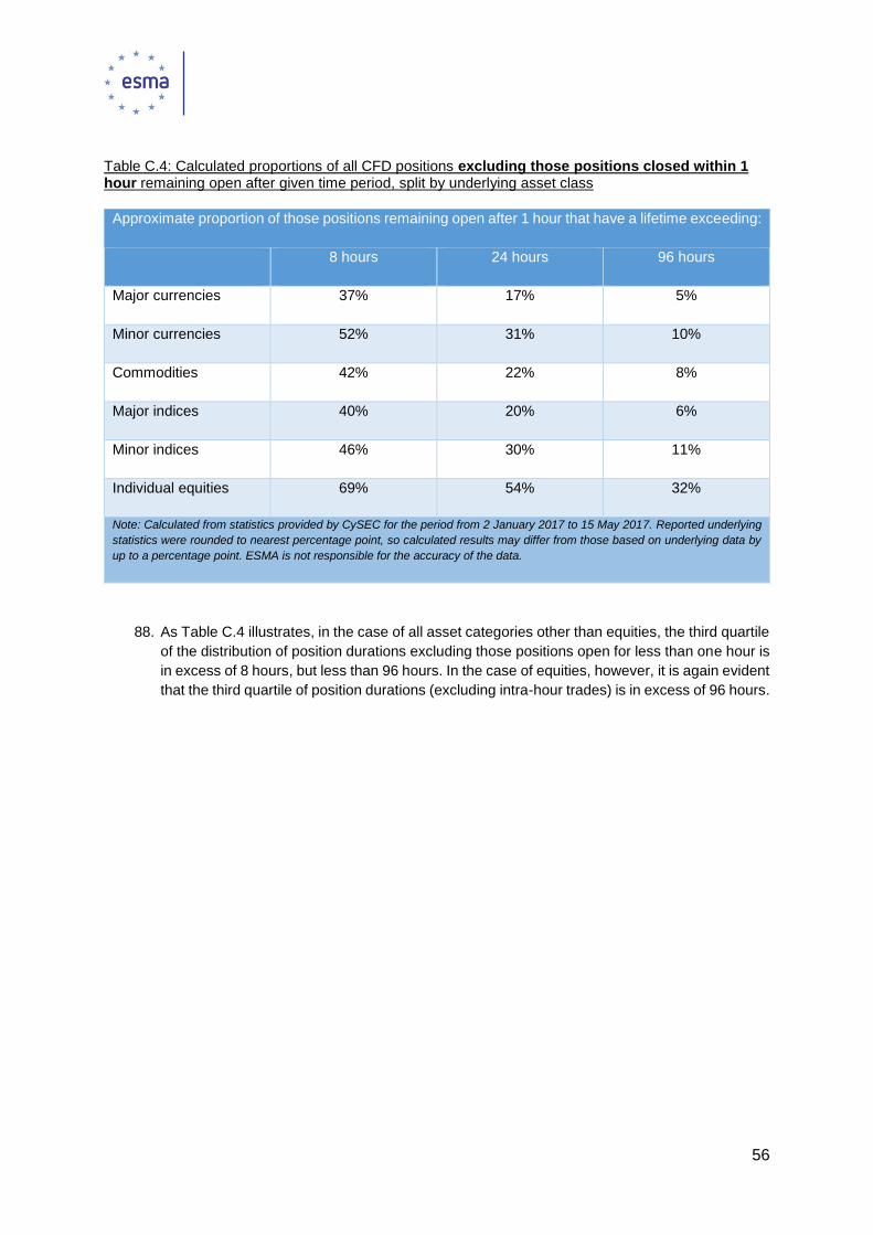
56
Table C.4: Calculated proportions of all CFD positions excluding those positions closed within 1 hour remaining open after given time period, split by underlying asset class
Approximate proportion of those positions remaining open after 1 hour that have a lifetime exceeding:
8 hours 24 hours 96 hours
Major currencies 37% 17% 5%
Minor currencies 52% 31% 10%
Commodities 42% 22% 8%
Major indices 40% 20% 6%
Minor indices 46% 30% 11%
Individual equities 69% 54% 32%
Note: Calculated from statistics provided by CySEC for the period from 2 January 2017 to 15 May 2017. Reported underlying
statistics were rounded to nearest percentage point, so calculated results may differ from those based on underlying data by
up to a percentage point. ESMA is not responsible for the accuracy of the data.
88. As Table C.4 illustrates, in the case of all asset categories other than equities, the third quartile
of the distribution of position durations excluding those positions open for less than one hour is
in excess of 8 hours, but less than 96 hours. In the case of equities, however, it is again evident
that the third quartile of position durations (excluding intra-hour trades) is in excess of 96 hours.

57
89. A point to stress is the extreme heterogeneity in the available data. This heterogeneity is
illustrated by the case of data from a second large UK-based CFD firm, provided to ESMA by
the UK FCA, for which the third quartile of trade durations were as follows.53
Table C.5: Statistics on third quartile of trade durations by asset class
Third quartile of reported trade durations
Currencies 22 days
Commodities 47 days
Indices 13 days
Individual equities 142 days
Note: Calculated from statistics reported by a large UK-based provider covering all positions closed in the period 1 March 2017
to 1 June 2017. ESMA is not responsible for the accuracy of the data.
90. These data support the finding that according to the evidence available, there is a substantial
population of retail investors who hold CFDs in excess of an intra-day trading period.
91. While durations of trades according to this large firm in question tend to be significantly longer
than those from reported from the other sources, a clear feature in common is that the durations
for equity share CFDs tend to be much the longest among the different asset classes. To take
a specific metric, the third quartile holding period for equities in this sample of data can
straightforwardly be calculated to be 5.2 times that of the mean of the third quartiles across the
other asset classes.
92. A final point to note in relation to interpreting the range of durations presented in this document
is that patterns of trading and investment behaviour may themselves change as a result of the
introduction of leverage limits or other measures. ESMA does not have evidence to quantify
the likely size and direction of any such effects, however.
53 As the holding periods for these assets were very long in general, the results are not materially affected if intra-hour holdings are excluded, and so for the statistics for the full dataset are simply presented.

58
4.1.5 Asset selection
93. The assets modelled were selected as follows.
94. The set of equities comprises the 6 largest US companies (Apple, Alphabet (Google), Microsoft,
Amazon, Berkshire Hathaway, Facebook); the 6 largest European-based companies: Nestle
(Switzerland), Anheuser-Busch Inbev (Belgium), Roche (Switzerland), Royal Dutch Shell (UK),
Novartis (Switzerland), HSBC (UK); and the largest 3 from the rest of the world: Tencent
(China), Alibaba (China), Samsung (South Korea), as measured by market capitalisation as of
March 2017.54
95. The set of major currencies is based on the 6 most-traded currencies globally by volume,
according to price data provided by an NCA, as of October 2017. All 15 possible pairs (without
double-counting the reverse of a pair, e.g. only including one out of EUR/USD and USD/EUR),
with the selection typically driven by data availability, feature in the results.
96. The set of minor currencies is a sample of currency pairs underlying CFDs offered by IG Group.
As many such currency pair CFDs are offered, the sample was selected based on currency
pair CFDs that were also prominently offered by two other large providers, namely CMC
Markets and Plus500.
97. The set of major indices takes indices which, according to knowledge of the market provided
by NCAs, and taking account of responses to the call for evidence, are highly traded or typically
regarded as major indices by firms and investors.
98. The set of minor indices comprises those remaining indices for which average spreads were
available on the website of IG Group and for which the relevant data were available from
Thomson Reuters.
99. Among commodities, the two most-traded assets in futures market, by some margin, according
to data provided by an NCA as of October 2017, were gold and crude oil. This proxy for investor
trading is confirmed by market intelligence based on NCA discussions with firms. These assets
are key in terms of intervention calibration – indeed, taking into account historic market prices,
gold has been assigned a separate leverage limit to other commodities. For this reason, Chart
1 in Section 3 presents the results for gold and (Brent crude) oil separately to the other
commodities modelled. To provide additional information, a large set of other assets was
selected based on the list of available assets (numbering 40 in total) from the website of IG
Group. Assets were selected to include those most prominently displayed on the website, which
other than gold, Brent crude oil and West Texas Intermediate oil included silver, wheat, natural
gas and sugar.55 In several cases, more than one contract was quoted for the same commodity,
in which case (with the exception of crude oil) at most one contract was modelled.
100. The set of cryptocurrencies selected were those offered by IG Group as of February
2018 for which data were available. As of March 2018, Bitcoin was the largest cryptocurrency
by market capitalisation, followed by Ether, followed by Ripple.
54 Source: PwC, 2017: “Companies by market capitalization – 31 March 2017 update”. Available at http://www.pwc.com/top100
55 Commercially available market-wide data provided by an NCA on exchange-traded volumes of standard commodities contracts for the first 9 months of 2017 showed that around USD 48bn of Brent oil futures were traded and around USD 35bn for gold. Third was gasoline, at around USD 14bn and fourth was natural gas, at USD 13bn. All of these assets were included in the sample.