Product Evaluation for Performance and the Effects of Variation

l to compare the performance of the product to the engineering specifications (or targets) developed earlier in the design project

l The process of Product Evaluation– Monitoring functional change– Goals of performance evaluation– Accuracy, variation, and noise– Modeling for performance evalution– Tolerance analysis– Sensitivity analysis– Robust design– Design for cost (DFC)– Value Engineering– Design for manufacture (DFM)– Design for assembly (DFA)– Design for reliability (DFR)– Design for test and maintenance– Design for the environment

Functional Evaluation

l Benefits in refining the function model as the form is evolving– The functions that the product must accomplish can be kept very clear

by updating the functional breakdown.• Nearly every decision about the form of an object adds something, either

desirable or undesirable to the function of the object.– Tracking the evolution of function means continuously updating the flow

models of energy, information, and materials.• These flows determine the performance of the product.

In earlier design process:

Design Problems

Function models

Potential Concepts

Product Generation

Changes in functions and concepts

Goals of Performance Evaluation

l To evaluate the product design relative to targets set previously.l Factors must be supported by the evaluation of product performance:

– Evaluation must result in numerical measures of the product for comparison with the engineering requirement targets developed during the problem understanding.

• Measurements must be of sufficient accuracy and precision for valid comparison.

– Evaluation should give some indication of which features of the product design to modify; and by how much in order to bring the performance on target.

– Evaluation procedures must include the influence of variations due to manufacturing, aging, and environmental changes.

• Insensitivity to these “noises” while meeting the targets results in a robust, quality product.

l Additional concepts for better design:– Optimization; trade studies, accuracy, tolerances, sensitivity analysis and robust design

P-Diagram

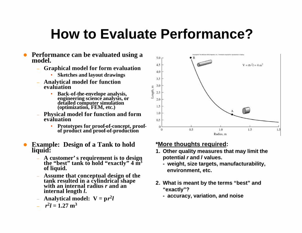
How to Evaluate Performance?l Performance can be evaluated using a

model.– Graphical model for form evaluation

• Sketches and layout drawings – Analytical model for function

evaluation• Back-of-the-envelope analysis,

engineering science analysis, or detailed computer simulation (optimization, FEM, etc.)

– Physical model for function and form evaluation

• Prototypes for proof-of-concept, proof-of product and proof-of-production

l Example: Design of a Tank to hold liquid:

– A customer’s requirement is to design the “best” tank to hold “exactly” 4 m3

of liquid.– Assume that conceptual design of the

tank resulted in a cylindrical shape with an internal radius r and an internal length l.

– Analytical model: V = πr2l– r2l = 1.27 m3

*More thoughts required:1. Other quality measures that may limit the

potential r and l values.- weight, size targets, manufacturability,

environment, etc.

2. What is meant by the terms “best” and “exactly”?- accuracy, variation, and noise

Accuracy, Variation, and Noisel The purpose of modeling is to find the easiest method by which to evaluate the product

for comparison with the engineering targets using available resources.l Two types of errors in any model

– Errors due to inaccuracy– Errors due to variation

l Accuracy– The correctness or truth of the model’s estimate– In case of distributed results, the best estimate (mean) will be a good predictor of product

performance.– The variation in the results obtained from the model refers to statistical variation of the

results about the mean value.• Precision, resolution, range and deviation are also used to refer to the distribution of the evalution.

– The obvious goal in modeling is to develop an accurate model with a small variation.– Accuracy tells “how much” whereas distribution tells “how sure”.

l Why concern the variation?– Each parameter that defines the product or process has variation and so each may vary

greatly from the desired mean.

Examples of Variation

l Remember that, during production, not all samples of the product:

– are exactly the same size;– are made of exactly same material;

or– behave in exactly the same way.

l We have to consider how such variations affect the performance in the design process.

– Deterministic analytic models– Non-deterministic (or stochastic)

analytical models that account for both the mean and the variation by using methods from probability and statistics

Effect of Variation on Product Quality

l A product is considered to be of high quality if its quality measures stay on target regardless of parameter variation due to manufacturing, aging, or environment.

l Control parameters vs. Noise as a source of variation

– Control parameters:• parameters controllable by the

designer, such as working environment, geometry, etc.

– Noise:• Uncontrollable parameters• Noises affecting the design parameters

– Manufacturing, or unit-to-unit variations

– Aging, or deterioration, effects, including etching, corrosion, wear and other surface effects

– Environmental, or external, conditions including all effects of the operating environment.

How to Deal With Noisesl Noises that affect the strength are often accounted for by using a “safety factor

(or factor of safety).”– FS = Sal/σap (Sal = allowable strength; σap = applied stress)– Rule-of-Thumb Factor of Safety (see appendix C)

l Keep noises small by tightening manufacturing variations (generally expensive)l Add active controls that compensate for the variations (generally complex and

expensive).l Shield the product from aging and environmental effects (sometimes difficult

and may be impossible).l Make the product insensitive to the noises (robust design).

– Key Philosophy of Robust Design:• Determine values for the parameters based on easy-to-manufacture tolerances and

default protection from aging and environmental effects so that the best performance is achieved. The term, best performance, implies that the engineering targets are met and the product is insensitive to noise. If noise-insensitivity cannot be met by adjusting the parameters, then tolerances must be tightened or the product shielded from the effects of aging and environment.

Modeling for Performance Evaluation

l Steps to give order to the considerations taken into account during evaluation:1. Identify the output responses (i.e., critical or quality parameters) that

need to be measured.2. Note how accurate the output needs to be.3. Identify the input signal, the control parameters and their limits, and

noises.4. Understand analytical modeling capabilities.5. Understand the physical modeling capabilities6. Select the most appropriate modeling method.7. Perform the analysis or experiments.8. Verify the results.

Tolerance Analysis

l Theoretically, tolerance is assumed to represent ±3% standard deviations about the mean value, implying that 99.68% of all the samples should fall within the tolerance.

l Focus of tolerance design is the concern about tolerances on dimensions and other variables (i.e., material properties) that affect the product.

– It is shown that only a fraction of the tolerances on a typical component actually affect its function.

Effect of Tighter Tolerances on the Manufacturing Cost

*Specification of tighter tolerances will increase the manufacturing cost.- use nominal tolerance whenever possible.

Meaning of the Tolerances Specified on the Drawings:

1. It communicates information to manufacturing that is essential in helping to determine the manufacturing processes that will be used.

2. Tolerance information is used to establish quality-control guide-line. (conformance quality)

Additive Tolerance Stack-upl Most common form of tolerance

analysis.

*Example of Air shock-swingarm:When the joint is assembled,

lg = ls – (lb + 2 x lw)

lg = gap lengthls = distance between fingerslb = bushing lengthlw = washer thickness

Worst-case Analysis:If lb = 19.97 (min), lw = 1.95 (min), ls = 24.1 (max), thenlg = 0.23 mm.If lb = 20.03 (max), lw = 2.05 (max), ls = 23.9 (min), thenlg = -0.23 mm (interference).

If you want assembly to be easy, no interference, thenYou should specify ls = 24.33 ± 0.1 mm so that the narrowest possible distance between the fingers will still fit the widest components.

Statistical Stack-Up Analysisl A more accurate estimate of the gap can be found statistically, in a form of statistical analysis.l Consider a stack-up problem composed of n components, each with mean length li and tolerance ti (assumed

symmetric about the mean).

In general, a length of the dependent parameter is,

l = l1 ± l2 ± l3 ± … .. ± lnthe sign on each term depends on the structure of the device.

The standard deviation is

s = (s12 + s2

2 + s32 + … .. + sn

2)1/2

Since s = t / 3,

t = (t12 + t22 + t3

2 + … .. + tn2)1/2

l For the example,

lg = ls – (lb + 2 x lw), tg = (ts2 + tb

2 + 2 x tw2) ½

For ls = 24.00 ± 0.1, lb = 20.00 ± 0.03, lw = 2.00 ± 0.05;

lg = 24 – (20 + 2 x 2) = 0.0 and tg = (0.102 + 0.032 + 2 x 0.052) 1/2 = 0.126 mmOn the average, there is no gap and the tolerance on it is 0.126 mm.

Example of Statistical Stack-Up Analysisl For the example of Air shock-swingarm,

lg = ls – (lb + 2 x lw), tg = (ts2 + tb

2 + 2 x tw2) ½

For ls = 24.00 ± 0.1, lb = 20.00 ± 0.03, lw = 2.00 ± 0.05;

lg = 24 – (20 + 2 x 2) = 0.0 and tg = (0.102 + 0.032 + 2 x 0.052) 1/2 = 0.126 mm

On the average, there is no gap and the tolerance on it is 0.126 mm.

In this problem, let’s make further assumptions:1) When bolted, the fingers can flex up to 0.07 mm inward without undo stress on the welds

to compensate for any clearance.2) The assembly personnel can get the parts in between the fingers even if there is a 0.03

mm interference.Then, what percentage of the assemblies will meet these requirements?

Figure shows that the probability for problems to occur during assembly is 29% (24 + 5).

How can we readjust the tolerance values?1) Inspect each part and reworking on the

numbers.2) Determine which tolerance is most sensitive to

the results using sensitivity analysis and repeat the tolerance analysis.

Sensitivity Analysisl Technique for evaluating the statistical relationship of control

parameters and their tolerances in a design problem.– Sensitivity analysis allows the contribution of each parameter to the

variation to be easily found

l For 1-dimensional problem (air shock-swingarm):s = (s1

2 + s22 + s3

2 + … .. + sn2)1/2

For Pi = si2 / s2, where Pi is the contribution of the i-th term to the tolerance (or variance) of the dependent

variable

1 = P1 + P2 + … .. + Pn

For air shock-swingarm problem;Ps = (0.1 x 0.1)/(0.126 x 0.126) = 0.63 = 63%Pb = (0.03 x 0.03)/(0.126 x 0.126) = 0.05 = 5%

Pw = (0.05 x 0.05)/(0.126 x 0.126) = 0.16 = 16% 0.63 + 0.05 + 2 x 0.16 = 1.00

- The tolerance on the spacing has the greatest effect on the gap. Thus, the tolerance on the spacing is the most likely candidate for change.

Multi-dimensional Sensitivity Analysis

)......,,,( ,321 nxxxxfF =

),.......,,,( 321 nxxxxfF =2/1

2221

2

1

)(......)(

∂∂

++∂∂

= nn

sxF

sxF

s

Consider a general function:

F = a dependent parameter (length, volume, stress or energy) andxi = the control parameters (usually dimensions and material properties)

For means and standard deviations (si),

If ∂F/ ∂xi = 1, this SD equation becomes a linear equation

Tank Problem

lrV 21416.3=

For the independent parameters of rand l, the mean volume is:

The tolerance on these parameters can be based on what is easy to achieve with nominal manufacturing processes.

Let tr = 0.03 m (sr = 0.01) and tl = 0.15 m (sl = 0.05), then SD on this volume is:

2

2/1

22

22

1416.3

2830.6

rlV

and

rlrV

where

srVs

lVs rlv

=∂∂

=∂∂

∂∂+

∂∂=

For point A, ∂V/ ∂r = 6.61 and ∂V/ ∂l = 4.60, so sv = [6.612 x 0.052 + 4.602 x 0.032]1/2 = 0.239

- 99.68% (3 SD) of all the vessels built will have volumes within 0.717 m3(3 x 0.239) of the target 4 m3.

For point B, ∂V/ ∂r = 16 and ∂V/ ∂l = 0.78, sosv = [0.782 x 0.052 + 162 x 0.032]1/2 = 0.166

- 99.68% (3 SD) of all the vessels built will have volumes within 0.498 m3

of the target 4 m3.

*Reduction in variation can be achieved not by changing the tolerances on the parameters but by changing only their nominal values.

*If we can find the values of r and l that give the smallest variance on the volume, then we are employing the philosophy of robust design.

Robust Design by Analysisl In the previous tank example, the tank with greater length had less sensitivity to

the large tolerance on the length, so the tank volume varies less.l What are the most robust values for the parameters?

– It is impossible to have V = 4 m3, exactly due to random variations in r and l.– The best we can do is to minimize the difference between V and 4 m3.

( )

( ) ( ) )(2

....

var

222222

2

2

21

2

1

TlrsrsrlC

TFsxF

sxF

C

biasianceC

lr

nn

−++=

−+

∂∂++

∂∂=

×+=

πλππ

λ

λThe objective function to be minimized is:T = target

For the tank,

For known SDs on r and l, and known target T

( )

( )

40

220

24220

2

222

22322

−==∂∂

+==∂∂

++==∂∂

lrC

rsrllC

rlsrslrrC

r

lr

πλ

λππ

πλππ

31

22

414.1

=

=

r

l

l

r

ss

l

ss

lr

π

For sr=0.01, sl=0.05;

r = 0.71 m; l = 2.52 m; sv = 0.138 m3

Improvement in volume variation!*If this SD is not small enough, we need to tighten the tolerances of r and/or l.

Summary: Robust Designl Step 1: Establish the relationship between

quality characteristics and the control parameters. Also define a target for the quality characteristics.

l Step 2: Based on known tolerances (SDs) on the control variables, generate the equation for the standard deviation of the quality characteristics.

l Step 3: Solve the equation for the minimum SD of the quality characteristic subject to this variable being kept on target.

)......,,,( ,321 nxxxxfF =

2/1

2221

2

1

)(......)(

∂∂

++∂∂

= nn

sxF

sxF

s

Limitations on this method:1. It is only good for design problems that can be represented by an equation.2. The objective function used in the previous example does not allow for the

inclusion of constraints in the problem. For example, if the radius had to be less than 1.0 m because of space limitations, the previous cost function would need additional terms to include.

Robust Design Through Testingl Used when the quality characteristics cannot be represented in

an equation.– V = f(r,l), i.e., analytically in-deterministic relationship, as compared

with V = πr2l, analytically deterministic relationship– Begin by building a tank with some best-guess dimensions and measure

the volume. Repeat building a tank until we can find the right dimensions.

l Drawbacks:– Repetitive model building is not efficient.– There is no guarantee that the final design will be the most robust.

l Steps to overcome such drawbacks.1. Identify signals, noise, control, and quality factors (i.e., independent

parameters.2. For each quality measure (i.e., output response) to be evaluated, recall

or determine its target value and the nature of the quality loss function.3. Design the experiment.4. Take and reduce data.5. Analyze the results, and select new test conditions if needed.

Step 1: Identify signals, noise, control, and quality factors

Step 2: For each quality measure (output response), determine its target value and the nature of the quality loss function.

Quality loss is proportional to the mean square deviation (MSD), average difference between the output response and the target. This difference is often referred to as signal-to-noise (S/N) ratio.

∑=

n

iiy

n 1

21 ∑=

n

i iyn 12

11 ( ) ( )22

1

1myyy

n

n

ii −+−∑

=

− ∑=

n

iiy

n 1

21log10

− ∑=

n

iiy

n 1

21log10 ( )

−− ∑=

n

ii yy

n 1

21log10

Quality Loss Function: smaller-is-better larger-is-better Nominal-is-best

MSD

S/N Ratio