Product Engineering Optimizer Page 1 Product …bndtechsource.ucoz.com/V5_Online_Docs/Knowledgeware/kwoug2.pdf · Using the Design of Experiments Tool Tips and Tricks Advanced Tasks

Product Engineering Optimizer

Preface

Using this Guide

What's New

Getting Started

Basic Tasks

Using the Optimize Function Defining an Optimization Getting Familiar with the Optimization Dialog Box

The Problem Tab The Constraints Tab The Computations Results Tab To know more about the Computations results tab

Specifying the Algorithm to be Run Searching for a Maximum Value Searching for a Minimum Value Using the Gradient based Algorithm to Optimize Problems with non satisfied constraints Using Constraints Running a Constrained Optimization With Weights

Using the Constraint Satisfaction Function Using the Constraint Satisfaction Function Getting Familiar with the Constraints Satisfaction Editor Using Measured Parameters in a Constraint Satisfaction Computation

Using the Design of Experiments Tool Introducing the Design of Experiments Tool Getting Familiar with the Design of Experiments Window Using the Design of Experiments Tool

Tips and Tricks

Advanced Tasks

Interpreting Results Methodology Tips and Tricks

Optimal CATIA PLM Usability for Product Engineering Optimizer

Workbench Description

Product Engineering Optimizer Toolbar Constraint Satisfaction Toolbar

Customizing for Knowledgeware

Knowledge Tab Language tab Report Generation Tab

Glossary

Index

1Page Product Engineering Optimizer Version 5 Release 13

PrefaceOptimization plays a prominent role in structural design. The importance of minimum weight design of structures is recognized in most industries because the weight of the system affects its performance or because of the depletion of our conventional energy sources. But optimization is not only a matter of weight, it can be used to optimize any type of data. In real world engineering problems, it is also common to minimize an objective function describing data such as the total volume, the life-time or the cost of a structure.

The Product Engineering Optimizer is the CATIA answer to optimization. It provides engineers who design structures with an easy-to-use tool based on iterative methods. Using the Product Engineering Optimizer is mainly a question of practice and methodology.

The Product Engineering Optimizer can operate with two algorithms: the Conjugate Gradient and the Simulated Annealing. You select one or the other to run an optimization depending on the function to analyze. Although it is not required to have a prior preparation in optimization techniques, those of you who want to know in detail how these algorithms work can refer to the publications below:

● Numerical Recipes in C - The Art of Scientific Computing - ISBN - 0 - 521 - 43108 - 5, 1988 - 1992

● Nonconvex Minimization Calculations and the Conjugate Gradient Method, Powell, M.J.D., Lecture

Notes in Mathematics, Vol. 1066, pp. 122-141, 1984. [Advanced review on conjugate gradient for nonconvex functions.]

● Optimization by Simulated Annealings, Randelman, R. E., and Grest, G.S., N-City Traveling

Salesman Problem - , J.Stat. Phys. 45, 885-890, 1986.

● Function Minimization by Conjugate Gradients, Fletcher, R. and Reeves, C.M., Comp, J. 7, 149-154,

1964. [Advanced article on using conjugate gradient for nonconvex functions.]

ConventionsUsing this Guide


Using this GuideThis User's Guide is intended to help users become quickly familiar and efficient with the CATIA Version 5 Product Engineering Optimizer. Before reading it, users should be familiar with the basic CATIA Version 5 concepts, such as the document windows, standard toolbars and menus.

To get the most out of this guide, it is highly recommended to start reading and performing the tasks described in the step-by-step tutorial, known as the Getting Started section.

This User's Guide is organized into the following sections:

● Preface: a short introduction to the product.

● Getting Started: a step-by-step tutorial.

● Basic Tasks: a presentation of the most common tasks.

● Advanced Tasks: a presentation of more advanced product functions.

● Workbench Description: a presentation of the user interface.

● Glossary: a list of terms specific to Product Engineering Optimizer.


What's New?

New Functionality

Using Measured Parameters in Constraints SatisfactionsKnowledgeware parameters that are valuated by a formula are now taken into account by the constraint satisfaction function.

Multiple Solutions in Constraints SatisfactionsIt is possible for the user to find more than one solutions to a problem in the Constraints Satisfaction editor.

Optimal CATIA PLM Usability for Product Engineering Optimizer Safe save mode to ensure that data created in CATIA can be correctly saved in ENOVIA V5.


Getting Started

Let's take a simple example to introduce the CATIA Product Engineering Optimizer capabilities. Follow the step-by-step instructions described below to get a first appreciation of the CATIA Product Engineering Optimizer principles.

To know more about the optimization data as well as the algorithms to be run, see Defining an Optimization and Specifying the Algorithm to be Run.

The purpose of this task is to provide the user with a brief outline of how the optimizer works when searching for a target value in both operating modes. No computed data are given since:

● The behavior of the optimization process slightly depends on the platform. This is

particularly true for the Simulated Annealing algorithm.

● The algorithms are subject to changes from one version to the other.

Searching for a target value with the Simulated Annealing Algorithm

1. Open the KwoGettingStarted.CATPart document.

2. If need be:

❍ Check the Parameters and Relations options in the Display tab of the

Tools->Options...->Infrastructure->Part Infrastructure dialog box.

❍ Check the With Value, With Formula options in the Knowledge tab of the

Tools->Options...->General->Parameters and Measure dialog box.

❍ Check the Load Extended Language libraries and, under Packages to load, select

the PartDesign package or check All Packages in the Language tab. Click OK.


❍ Set the volume unit to cm3. To do so, select the Parameters and Measure

option and click the Units tab. In the Units table, select the Volume line and in the

scrolling list located below, select Cubic centimeter (cm3). Click OK to validate

your settings.

3. From the Start->Knowledgeware menu, access the Product Engineering

Optimizer workbench.

4. Click the icon. The Optimization dialog box displays.

5. In the Problem tab, fill in the fields with the data below:

Optimization type Target Value

Optimized Parameter Volume.1

Target value 800cm3

Free Parameters xA, yA, xB

Algorithm Simulated AnnealingConvergence speed: Fast

Don't modify the default termination criteria.

6. Check the Save optimization data check box, otherwise the optimization data won't be

saved.

7. Check the With update visualization check box. Don't fill in any field in the Constraints

tab.

8. Click Run Optimization.

❍ A file selection panel is displayed. Choose a path.

❍ Click Save to start the optimization process. A box displays the data computed for

each iteration. As the optimization is running, you can see the Volume.1 value

changing in the specification tree, if not, expand the Relations node in the

specification tree.


❍ After the computation has finished running, the Optimization dialog box displays

the values of the free parameters.

9. Click OK and save your document under a new name

Searching for a Target Value with the Gradient Algorithm

1. Re-open the KwoGettingStarted.CATPart document.

2. Repeat the same interactions as above but specify a Gradient algorithm in the

Optimization dialog box.

Don't fill in any field in the Constraints tab.

You need approximately 75 evaluations to reach a Volume.1 steady value. The target value is

reached quicker than in simulated annealing.

To know more about the Gradient and the Simulated Annealing algorithms, see Defining and Optimization.


Basic Tasks Using the Optimize Function

Using the Constraint Satisfaction FunctionUsing the Design of Experiments Tool

Tips and Tricks


Using the Optimization Function The following tasks are described in this guide:

Searching for a Maximum Value, Searching for a Minimum Value: Select the Optimize icon to perform an optimization.

Defining an OptimizationGetting Familiar with the Optimization Dialog Box

Specifying the Algorithm to be RunSearching for a Maximum ValueSearching for a Minimum Value

Using the Gradient Based Algorithm to optimize Problems with non satisfied constraintsUsing Constraints

Running a Constrained Optimization With Weights


Defining an Optimization Optimization is the process of searching for the minimum, maximum, or for a target value of an Objective function of one or several variables while satisfying certain restrictions or constraints.

A good example of optimization is the minimum weight design of structures in aerospace industry where aircraft structural designs often prevail on cost considerations. The notion of optimization presupposes that the operation to be improved or optimized is described by a function whose variation can be expressed with respect to a group of parameters, also called variables or free parameters.

Given f(x) a CATIA parameter expressed in terms of other CATIA parameters:

Min f(x, ..., xn)

such that:

gi (x1, ...) > Ki hj (x1, ..., xn) == Kj LB [ xi[ UB

Where:f(x) is a Knowledge Advisor formula (Optimization objective function).

= (x1, ..., xn)xi is a Knowledge Advisor parameter (Optimization free parameters).

g, h are constraints (optional).

Product Engineering Optimizer offers three operating modes whereby you can search for the:

● f(x) minimum,

● f(x) maximum,

● a given value of f(x) or a

● constraints satisfaction.

These operating modes are respectively called the Minimization, the Maximization and the Target Value modes.


Getting Familiar with the Optimization Dialog Box

The dialog box is displayed when you click the Optimize ( ) icon. It provides you with three tabs.

● The Problem tab

● The Constraints Tab

● The Computations results Tab

● In the optimization panel, the user can choose if the optimization is launched with or

without visualization update by clicking the With update visualization or the Without update visualization option.

● In non visualization mode (Without update visualization), performances have been

improved. Gains between both modes (With update visualization and Without update visualization) range from 15% to 40% depending on the models and the optimizations.


The Problem TabThe Constraints Tab

The Computation Results Tab


The Problem Tab

Optimization type


The list provides you with the:

● Minimization

● Maximization

● Target Value

● Only constraints

items which define the optimization type.

Optimized parameter

Click Select... to display the list of parameters that can be potentially optimized.

Free parameters

● To specify free parameters, click the Edit list... button.

● To specify bounds for a free parameter, select the parameter you want to add bounds to in the Free Parameters list, then click Edit ranges and step.... The dialog box which is displayed also allows you to specify a step (see picture opposite.)

It is now possible to simultaneously valuate the ranges and steps of several free parameters. To do so, proceed as follows:

1. Select 1 free parameter and apply it ranges and/or steps (unchanged). 2. Select several free parameters and click the Edit Ranges and step button: The panel is filled with

the values of the first selected free parameter. All "Apply..." options are enabled.

Note that :

● To apply the same ranges and/or steps to free parameters, their types should be identical. If not, an


error panel displays.

● Note that if one of the "Apply this... to the selected parameters" check boxes is unchecked, the modifications performed (value changed or removed) on the corresponding range and/or the step will not be taken into account for the selected parameters. The old configuration is kept for each selected parameter. Therefore, if the user modifies the value (or removes it by unchecking the first check of the row) of a range or a step, and then unchecks the corresponding 'Apply this ... selected parameters' check box, the modification will not be taken in account. The selected parameters will keep their own values.

● If the Inf. Range check box is unchecked, the selected parameters will have no inferior range. It is also true for the Sup. Range and the Step.

● When selecting the free parameters, the associated parameters are highlighted in the Catia tree.

It is now possible for the user to edit the steps directly in the cells.

Available Algorithms

See Specifying the Algorithm to be Run.

Global Search vs. Local Search

Simulated Annealing (Global Algorithm) Gradient (Local Algorithm)

Equality constraints allowed Precision is managed as a termination criteria. x == A is fulfilled when abs(x - A) < precision

Equality constraints not allowed No precision

Can be run with constraints and no objective function Must be run with an objective function, with or without specified constraints.

Termination criteria

If you don't know how the objective function is going to behave, run the algorithm with the default values. If need be, you can always re-run the algorithm if the process seems to require more iterations.

Optimization data

To benefit from the optimization curves, save your optimization data. When the Save optimization data box is checked, clicking Run Optimization displays a file selection dialog box.


Note that when the With update visualization radio button is checked, the visualization is updated during the optimization process. If this radio button is unchecked, the visualization is not updated during the optimization process.


The Constraints Tab

The Constraints Tab Creating a constraint

To create a constraint, click the New... button (The editor displayed is familiar to those of you who use the Knowledge Advisor product.) Constraints cannot be regrouped. You must enter each constraint one by one. The only operators that you can use when specifying constraints are:

● == (only Simulated Annealing)

● <, > (both algorithms).

Once a constraint has been specified, its gap with respect to the value specified in the constraint is displayed. An icon indicates whether the initial value fulfills the constraint.

An additional column now lists the weight assigned to each constraint. The user can modify the weight in this column.

Activating a constraint

A constraint can be made active (True) or inactive (False) by using the Activity field. A deactivated constraint is ignored by the optimization algorithm.

Editing a constraint body

Click the Edit... button to access the Optimization Constraints Editor to modify the constraint body. Note that this Editor is similar to the


Formula Editor.

It is now possible for the user to modify constraints weights by using the Weight field. To do so, select the constraint in the list and enter a new weight in the Weight field.


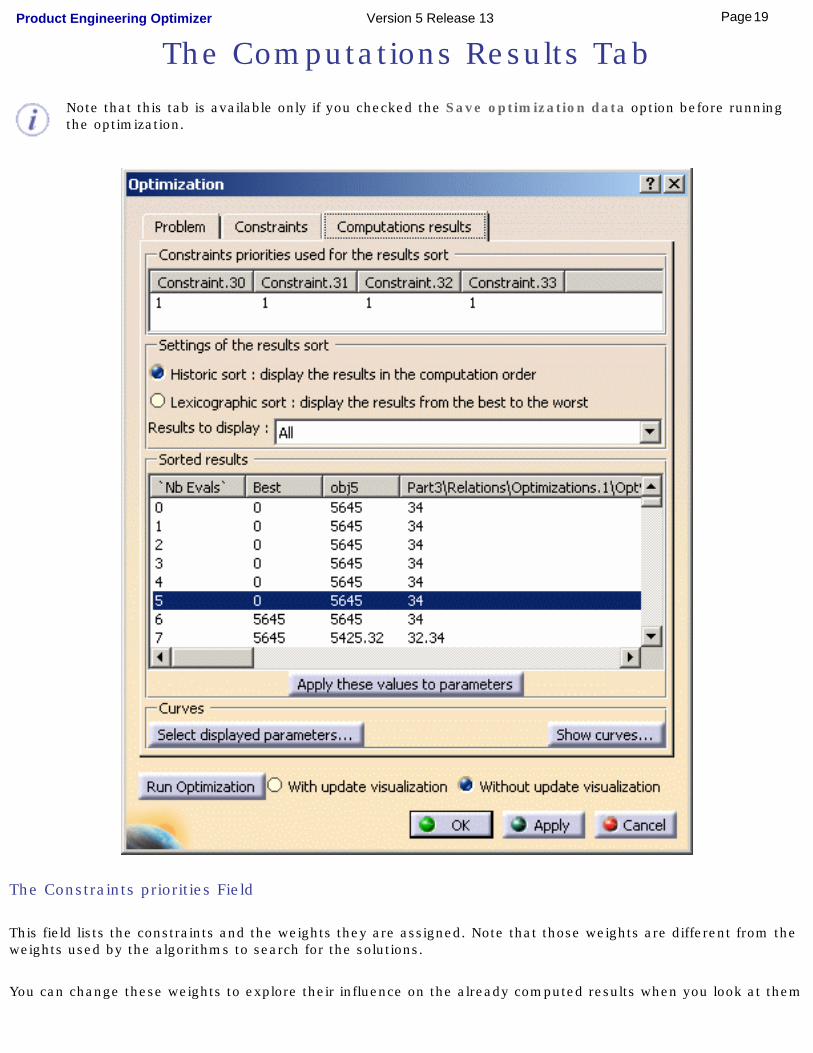
The Computations Results Tab

Note that this tab is available only if you checked the Save optimization data option before running the optimization.

The Constraints priorities Field

This field lists the constraints and the weights they are assigned. Note that those weights are different from the weights used by the algorithms to search for the solutions.

You can change these weights to explore their influence on the already computed results when you look at them


with the lexicographic sort. Changing those weights has no influence on the generated results i.e. they just present the existing ones under a new aspect.

Note that:● It is possible to edit constraints weights in this field. To do so, click the desired cell, and enter the

new weight.

● If you modify a constraint weight, the Sorted results list is automatically updated.

● Modifying a constraint weight in this tab will only impact the Lexicographic sort and not the algorithm. This may be useful to check the impact of a different weight without running the algorithm.

● If a weight is equal to 0, the default algorithm is used. 1 is the lowest weight that can be applied. There is no upper limit.

● Weights are reals (1.2 for example)

The Settings of the results sort Field

● Historic Sort: The results are displayed in the computation order.

● Lexicographic sort: The results are displayed going from the best to the worst, while taking the weights assigned to the constraints into account. To know more, see Running a Constrained Optimization With Weights.

Results to display scrolling list

● All: All results will display in the sorted list.

● All constraints satisfied only: Only the results concerning the satisfied constraints will display in the sorted list.

● User defined: Only the items selected by the user will display in the sorted list.

The Sorted Results Field

This list displays the result of the optimization according to the filters applied and the sorting type (Historic sort or Lexicographic sort).

The button enables the user to select a row in the list and to apply the values indicated in this row to the parameters.

The Curves Field

The button enables the user to select the parameters of the optimization file whose evolution will display in the curves. To know more, see Interpreting Results.


The Show curves... button enables the user to display the curves showing the parameters during the optimization process.

To know more, see To know more about the Computations results tab.


To know more about the Computations results tab

Algorithms Description

Simulated Annealing (global search):

All constraints are introduced at once in the algorithm. Priorities are handled by assigning weights corresponding to priorities to each constraint. A global function which regroups the objective and the modified constraints constitute the new objective function of the optimization.

Gradient Based Methods (Local search):

All the constraints must be differentiable as well as the objective function. The optimizer takes each constraint modified by its weight into account during the optimization process. The weights impact the search direction of the gradient.Thus in both cases modifying the weights might lead to different solutions for the same problem definition.

Exploiting Results: Filtering and Handling Weights

Priorities are handled at 2 levels:

● Constraints are handled a priori in the algorithms for better convergence.

● Weights are handled in the results post-processing in order to identify the best results according to the objective and constraints priorities. Constraints values are sorted from the highest to the lowest constraint priority starting from the highest priority.

● For two equivalent values of a given constraint the order is based on the next priority constraint (lexicographic order).

● When several constraints have equivalent priority a Pareto order is used to define the classification (i.e. a solution is equivalent to another solution if improving one constraint of same priority make (at least) another constraint worst. A solution is better if at least one constraint of the same priority is improved leaving the others unchanged or improved.).

Lexicographic order

Weights are all different

Constraints C1 C2 C3 Index # Class #

Weights 2 3 1 Values 10 20 30 1 5 10 3 2 2 2* 3 7 9 3 4 7 3 8 4 1* 3 6 8 5 3

In the table opposite, to know which row is the best, we first compare the values of c2 (highest weight: 3). If they are equal, we compare the values of c1 (example of Class # 2* and 1*) and so on in case of equality.


ConstraintsC1 C2 C3 Index #Class #Weights 2 1 3 2Values 10 20 30 1 5 10 3 2 2 1 (based on c1) 3 7 9 3 4 7 3 8 4 3* (based on c1 since c3

values are equal) 6 3 8 5 2*

In the table opposite, the C1 values must be taken into account since C2 and C1 values are equal.

● When weights are all equal, the only equivalence of 2 solutions occurs when all constraint values are equal between the 2 different solutions.

● Changing priorities changes the ranking of the solutions (Class #)

Some Weights are equal

ConstraintsC1 C2 C3 Index # Class #

Weights 1 2 2 Values 10 20 30 1 4 7 2 3 2 1* 3 7 9 3 3 7 3 2 4 1* 3 6 9 5 2

In the table opposite, if you consider only C1 and C2 values, 3 solutions are identical: 5, 4 and 2. Solution 3 is the intermediate solution and 1 is the worstIf you consider, all constraints, you get the following order, going from the best to the worst: 2, 4, 5, 3, 1.

* Both solutions are equivalent: When c2 increases, c3 decreases and conversely. Furthermore c1 is equal in both cases.

All Weights are equal

ConstraintsC1 C2 C3 Index # Class #

Weights 1 1 1 Values 10 20 30 1 2* 10 3 2 2 1 3 7 8 3 1 7 3 8 4 1 3 6 9 1

In the table opposite, all solutions are strictly equivalent except 2.

* All values are worse.

Analyzing Results


● The results of the optimization display in the Computations Results tab of the Optimization dialog box (2).

● Note that priorities are displayed in this tab and can be changed (1). Modifying a constraint weight in this tab will only impact the Lexicographic sort and not the algorithm.

● Several constraints can have the same priorities, results can be multiple (i.e. equivalent solutions). Those solutions are presented in decreasing order of significance.

● The #Class column is the quality of the solution(3). Solutions belonging to the same class are equivalent.

Filtering Results

The results list can be filtered in order to restrict the number of solutions displayed and to re-order solutions:

● Historic sort: The results are displayed in the order of exploration by the algorithm.

● Lexicographic sort: The solutions are sorted in lexicographic order (the highest weight first). In case of equivalence (i.e. constraints with same weights), they appear in historic order but with the same class.

Filters can also be applied to constraints values. A combo list enables the user to select the desired filter:

All: All solutions will display.

All constraints satisfied only: Only solutions with satisfied constraints will display.

User defined: Only the items selected by the user will display in the sorted list.

Selecting a Solution

It is possible to select a solution by clicking the and to apply it to the parameters.


Specifying the Algorithm to be Run

Types of Algorithm

To perform an optimization, you can use one of the algorithms below:

User algorithm defined in CAAOptimizationInterfaces

Users can define their own algorithms. To get an example, refer to the CAAOptimization interfaces.

Gradient algorithm

This algorithm should be used first to perform a local search. Based on the calculation of a local slope of the objective function this algorithm will use a parabolic approximation and jump to its minimum or use an iterated exponential step descent in the direction of the minimum.If the properties of the objective function are known (continuous, differentiable at all point), then the gradient can be used straight on. It is usually faster than the Simulated Annealing algorithm.

From this version on, users can choose to run the Gradient algorithm with constraints or without constraints.

Simulated Annealing based algorithm

● This algorithm is a global stochastic search algorithm hence two successive runs of this method might not lead to the same result. It performs a global search that evolves towards local searches as the time goes on.

● It is usually used to explore non-linear, multi-modal functions. These functions can also be discontinuous.

● If the shape of the objective function is unknown, it is recommended to start with a Simulated Annealing then refine the results with a gradient descent. This approach is slow but works for a larger amount of functions.

A good way to quickly reach a solution when using the Simulated Annealing consists in specifying a low number of consecutive iterations without improvements (15 or 20).

Each algorithm - the Gradient based algorithm and the Simulated Annealing algorithm - can be run in 3 different configurations (4 for the Simulated Annealing algorithm) corresponding to different behaviors:

● Slow

● Medium

● Fast

● Infinite (Hill climbing) (for Simulated Annealing only)


Name Gradient Algorithm Simulated Annealing Algorithm

Slow Slow evolution based on steps or bounds. Good precision (to be used to find convergence.)

These 4 configurations define the level of acceptance of bad solutions.If the problem has many local optima, use Slow.If the problem has no local optima, use Infinite (Hill climbing).

Medium A randomly restarted conjugate gradient.

Fast Search jumps from Minimum to Minimum.Fast evolution, less precision.

Infinite (Hill climbing) -

Termination Criteria

Termination criteria are used to stop the optimizer. When an optimization is running, a message box displays the data of each iteration. You can stop the computation by clicking Stop. If you don't intervene in the computation process, the computation will stop:

● When a value (minimum, maximum or target value) has been found and the algorithm is unable to

progress anymore (Gradient.) or

● When one of the specified termination criteria has been met.

Here are the termination criteria to be specified:

● Maximum number of iterations i.e. the number of times the objective function will be calculated at

most (number of updates.)

● Number of iterations without improvement i.e. the number of updates allowed without achieving a

better result.

● Maximum duration of computation

Simulated Annealing always runs until one of the termination criterion is reached. The Gradient can stop before if a local optimum is reached.

Algorithms Versions

From time to time, the PEO algorithms are updated to enhance their performances or to correct some bugs. The side effect of these modifications is a change of behavior of the optimization process. It is however possible to come back to the previous versions of the algorithms by using environment variables (see table below.)


Var Nam Var Value

GradientVersion R8Sp3, R9sp4, R10sp1, R11ga

SAVersion R8sp3

GradientWithCstVersion R8sp4, R11ga


Searching for a Maximum Value

This scenario illustrates the Maximization optimization type. The algorithm searches for the parameter values corresponding to a maximum value for Function2. The Simulated Annealing method is used. Lower and upper bounds (-10 and +10) are specified for the x argument.

1. Open the KwoGoal0.CATPart document or add to any document the parameters and

formulas described in the specification tree below:

2. From the Start->Knowledgeware menu, access the Product Engineering Optimizer

workbench and click the Optimize icon ( ). The Optimization dialog box is displayed.

3. Define the data required to run the optimization algorithm as follows:

Optimization type Maximization

Optimized Parameter Function2

Free Parameters x - Inf. Range: -10 ; Sup. Range: +10

Algorithm Simulated Annealing -Convergence speed: Fast

Maximum number of updates 200

Consecutive updates without improvements 50


Maximum time (minutes) 5 minutes

4. Check the Save optimization data box, otherwise your optimization data won't be saved

and you won't able to display the optimization curves.


❍ A file selection panel is displayed. Choose a path.

❍ Click Open. The optimization process starts. A panel displays the data computed for

each iteration. As the optimization is running, you can see the Function2 and x values

changing in the specification tree.

❍ A steady value of 500 is reached very early for Function2.

The free parameters as well as the Function2 value are updated in the specification

tree.

Note that Real type parameters are displayed with nine decimal

places (trailing zeros if any are not displayed). If you carry out an

optimization with other parameter types, the values will be

displayed according to the settings specified in the Units tab of the

Tools->Options... dialog box (General - Parameters and

Measure).

6. Replay the same scenario with a maximum number of updates of 50, then 20.

7. Click OK or Cancel to exit the Optimization dialog box.


Searching for a Minimum Value

The scenario below illustrates the Minimization Optimization type. The algorithm searches for the parameter values corresponding to a minimum value for Function2. The Gradient method is used.

1. Open the KwoGoal0.CATPart document or add to a document the parameters and formulas described in the

specification tree below.

The x, y, z, Function1 and Function2 parameters must be of real type. You don't need to specify their initial

values.

If need be, refer to the CATIA Knowledge Advisor User's Guide for information on how to create parameters and

formulas.

2. From the Start->Knowledgeware menu, access the Product Engineering Optimizer workbench and click the

Optimize icon ( ). The optimization dialog box is displayed.


Optimization type: Minimization

Optimized parameter: Function2

Free Parameters: x

Algorithm: Gradient

Maximum number of updates : 400

Consecutive updates without improvements: 100

Maximum time (minutes): 5 minutes


a. The Optimization message box displays the data for each iteration. Don't intervene on the algorithm


process (i.e. don't click Stop at the next iteration) and let the optimization process execute until the target

value is found out or one of the termination condition is reached.

b. The x parameter as well as the Function2 value are updated in the specification tree.

Note that Real type parameters are displayed with nine decimal places (trailing zeros, if any,

are not displayed). If you carry out an optimization with other parameter types, the values

will be displayed according to the settings specified in the Units tab of the Tools-

>Options... dialog box (General -> Parameters and measure).

The x value (10) resulting from the computation is displayed in the optimization dialog box.


Using the Gradient based Algorithm to Optimize Problems with non satisfied constraints

This task explains how to use the Gradient based Algorithm to optimize Problems with non satisfied constraints.

1. Open the KwoGettingStarted.CATPart file.


workbench.

3. Click the Optimize icon ( ) to access the Optimization dialog box. The Optimization

dialog box displays.

4. Enter the parameters below in the Problem tab:

Optimization Type Target Value

Optimized Parameter Volume.1

Target Value 800000mm3

Free Parameters

Algorithm Gradient - Fast

Termination Criteria

● Maximum number of updates

● Consecutive updates without improvements

● Maximum Time (minutes)

200

50

5

5. Enter the following constraints in the Constraints tab:


Constraint.1 Z**2 + Y**2 < 5000 mm2

Constraint.2 Y**2 + Z**2 > 1000 mm2

6. Click the Run Optimization button. The part should look like the one below once the

optimization process is over:

Click the graphic opposite to enlarge it.

7. Redefine the ranges of the free parameters (see below):

Free Parameters

8. Click the Run Optimization button. The generated values are much closer to the

Target value.


Click the graphic opposite to enlarge it.


Using Constraints

In the scenario developed below, the simulated annealing algorithm is used with constraints and without objective function to search for a set of xA, xB, yA and yB parameters so that the inertia axis of the pad remains within an area defined by two circles.Here are the circle definitions as they are specified as constraints in the scenario below:Y**2 + Z**2 < 8100mm2Y**2 + Z**2 < 1000mm2

After this part of the scenario has complete, the gradient algorithm is used to find a set of xA, xB, yA and yB so that the distance of the inertia axis to the origin is minimum. This second part of the scenario requires that the constraints are fulfilled.

Note that it is possible to use constraints without objective (Simulated Annealing only) or with objective (available for both algorithms.)

1. Open the KwoGettingStarted.CATPart document. This document is a pad extruded from

a spline. The relations defined in this document allow you to specify the position of an

inertia axis.



Optimizer workbench and click the Optimize icon ( ). The optimization dialog box

is displayed.

3. Select the Only constraints optimization type.

4. In the Problem tab, enter the free parameters below:

xA, xB, yA, yB. Don't select any optimized parameter.

5. Check the Simulated Annealing box.

6. In the Constraints tab, use the New... button to enter the constraint below

Y**2 + Z**2 > 8100mm2

7. Click OK in the constraint editor, then click New... again to enter the second constraint:

Y**2 + Z**2 < 10000mm2

8. In the Problem tab, click Run Optimization.

After the optimization has finished running, you obtain a pad whose inertia axis is

located in an area delimited by the two circles specified. Take a look at the Constraints

tab. The constraints are all fulfilled. You can now start a gradient algorithm to search for

the minimum value of the Rad parameter.

9. Click the Optimize icon ( ). In the Problem tab, select:

❍ Minimization as the optimization type.

❍ Rad as the parameter to be optimized and choose the Gradient algorithm.

❍ Don't modify the free parameters.

10. Run the optimization with the default termination criteria. After the optimization has

finished running, the minimum value of Rad is closed to 90mm. You have found a set of

xA, xB, yA, yB value so that the inertia axis of the pad is located almost on the circle

defined by the relation below:

Y**2 + Z**2 = 8100mm2


Running a Constrained Optimization With Weights

This task shows the user how to assign weights to constraints and how it can affect the geometry. The file provided is made up of a triangle. The scenario is divided into 2 steps:

● The user first wants to run the optimization so that the distance between the triangle vertex and Point.1 is as short as possible.

● Then the user wants to run the optimization so that the distance between the triangle vertex and Point.2 is as short as possible.

To do so, he defines constraints and assign weights to these constraints.

1. Open the KwoConstraintswithWeights.CATPart file. The following image displays:

This file contains a triangle. The

sides of the triangle are assigned

parameters valuated by formulas.

❍ f1: Distance between Point.1

and Point.3. It is valuated by

Formula.1.

❍ f2: Distance between Point.2


Formula.2.

❍ l1: Distance between Point.1


Formula.3.

❍ l2: Distance between Point.2


Formula.4.


workbench and click the Optimize icon ( ). The Optimization dialog box is displayed.



In the Problem tab

❍ In the Optimization type scrolling list, select the Only constraints option.

❍ Click the Edit list... button in the Free Parameters field. Use the arrow key to

select the following parameters and click OK when done:

■ Geometrical Set.1\Point.3\X

■ Geometrical Set.1\Point.3\Z

❍ In the Algorithm type scrolling list, select Simulated Annealing Algorithm.

In the Constraints tab

❍ Click the New... button to create a new constraint and enter the following script

into the editor:

f1*f1==0

❍ Click OK when done.

❍ Click the New... button to create a new constraint and enter the following script

into the editor:

f2*f2==0

❍ Click OK when done. The constraints are defined.


❍ Assign a weight to Constraint.1. To do so, click Constraint.1 in the table and

enter 5 in the Weight field.

❍ Keep the default precision value (1)

4. Click the With update visualization radio button and click the Run Optimization

button. Enter the name of the file that will contain the optimization data in the Save as

dialog box: Constraintswithweights.xls, and click Save.

❍ The Optimization message box displays the data for each iteration. Do not intervene

on the algorithm process (i.e. don't click Stop at the next iteration) and let the

optimization process execute until the target value is found out or one of the

termination condition is reached.

❍ The result

displays in the

Constraints tab.

❍ The geometry is

updated. The

representation of

Point.3 tends to

the right.

❍ Point.3 coordinates are updated in the specification tree.

5. Assign a weight to Constraint.2. To do so, click Constraint.2 in the table and enter 10 in

the Weight field.


6. Click the Run Optimization button. Click Yes when asked if you want to overwrite

Constraintswithweights.xls.

The result

displays in the

Constraints

tab.

The geometry

is updated. The

representation

of Point.3

tends to the

left.

Point.3 coordinates are updated in the specification tree.

7. Click the Computations results tab. The results are sorted in the Sorted results table (see

graphic below).


Note that you can:● Apply values to parameters.

● Select the parameters that you want to display in a curve.

● Display curves.


Using the Constraint Satisfaction Function The following tasks are described in this guide:

Using the Constraint Satisfaction Function: Select the Constraint satisfaction icon to solve a set of constraints using operators, functions and measures.

Using the Constraint Satisfaction FunctionGetting Familiar with the Constraints Satisfaction Editor

Using Measured Parameters in a Constraint Satisfaction Computation


Using the Constraint Satisfaction Function

This task explains how to solve a set of constraints using operators, functions and measures. This scenario can be run from any document.

● The syntax of this feature is the same as the one of the set of equations.

● Note that the constraint satisfaction capabilities require the PEO product.

1. Create a pad with a rectangular base.

2. Use the Formula editor to create a Volume parameter.


workbench.

4. Click the Constraint Satisfaction icon ( ). In the first dialog box which is displayed,

enter the name of the relation, and a comment (optional). Click OK.

5. Enter the set of equations below into the edition box:

Volume==smartVolume (PartBody\Pad.1 );PartBody\Pad.1\FirstLimit\Length >= 1mm;PartBody\Pad.1\FirstLimit\Length <= 1000mm

Now, your editor looks like this:

5. Click the Parse arrow ( ). At this step the editor identifies the variables of the set of

constraints and puts them as Unknown parameters.


● Before solving, select the parameters that will be considered as

input (constant) and the parameters that will be considered as variables by the solver.

● The value of the input parameters must be set to the desired

values.

6. Select the Volume parameter and use the arrow to move it to the Constant

parameters column.

7. Change the value of the Volume parameter. To do so, click twice (slowly ) inside the Value

cell and set the value to 0.003 M3. Click Apply. The following box displays:


The pad height is modified by the constraints satisfaction solver in order to match the given volume (0.003 M3).

8. This process can be reversed: The input parameters can be transferred to outputs and

vice-versa using the Switch input/output arrow ( ).

It is now possible to change the value of the Pad height and obtain the volume as a result.


A constraint satisfaction feature is not a conventional relation feature (like rules, checks, and formulas). It is an asynchronous feature (as the optimization.) Although input and output parameters are defined, changing an input outside the Constraint satisfaction editor does not trigger the solving process.

Like sets of equations and unlike optimization, constraint satisfaction issues an "unresolved system" warning if the solver is unable to satisfy all the equations and inequations.

If a set of constraints cannot be satisfied, you can relax the equality constraints by using a double inequality.

Volume+epsilon<=smartVolume (PartBody\Pad.1 );Volume-epsilon>=smartVolume (PartBody\Pad.1 );PartBody\Pad.1\FirstLimit\Length >= 1mm;PartBody\Pad.1\FirstLimit\Length <= 1000mm;

Using the Constraint Satisfaction Editor


Getting Familiar with the Constraints Satisfaction Editor

The dialog box is displayed when you click the Constraint Satisfaction ( ) icon. It is made up of three tabs.

● Editors tab

● Results tab

● Options tab

Editors tab

The Editor is divided into 3 main fields:

● The constraints body, i.e. their textual representation

● The Inputs and Outputs of the constraints

● The Dictionary of parameters and functions


● Constant parameters:

The values of constant parameters are set by the user and are considered as constant by the solver. This value can be changed directly in the Value column by clicking twice (slowly) in the Value cell.


● Unknown

parameters: The value of unknown parameters will be calculated once the Solve button is pushed.

The Parse arrow is used to identify the variables of the set of constraints. It must be pushed before choosing input and output variables.

The left arrow is used to move variables from the Unknown parameters category to the Constant parameters one.

The right arrow is used to move variables from the Constant parameters category to the Unknown parameters one.

The Switch input/output arrow is used to swap the selected constant and unknown parameters.

Click the Solve button to launch the computation.

Click Apply to launch the update of the model.

Results tab

Note that you can now find more than one solution to a single problem. To get an example, see Using Measured Parameters in a Constraint Satisfaction Computation.


Solution Distance: Enter the distance between the different solutions that you want to find.

Number of solutions to be found: Enter the number of solutions to be found.

This field displays each constraint identifier in the body.


This field displays the parameters taken into account by the computation and shows the solution found.

Select one of the solutions and click the Apply solution button. The solution is automatically applied to the geometry and the parameters are valuated with those of the solution.

Click this button if you want to save the result of the computation. Note that the results of the computation can be saved either in .txt or .xls format.

Options tab

Black box refers to a measure function. For instance, smartVolume is a measure that calculates the volume of a body.

● Use the Gauss method for linear equations: Accelerates the solve operation when working with linear equations.

Algorithm

● Precision: Enables you to define the precision of the results (i.e the number of decimal digits after the decimal point.) This precision is used when comparing 2 numbers. This option defines whether they are equal or not. When dealing with units, the comparison is made on the basis of the MKS value of parameters.


● Maximal computation time (sec.): Enables you to indicate the computation time. If the indicated time is equal to 0, the computation will last until a solution is found.

● Show 'Stop' dialog: If checked, displays a

"Stop" dialog box that will enable you to interrupt the computation.

Generate expanded error description: Enables you to get detailed information about errors if they occur.

Show additional warnings:

Black boxes algorithm: You have the choice between 2 algorithms. If your problem behaves like quadratic functions, select Quadratic approximation.


● Width: This parameter sets the minimal width of

the interval of unimodality for measures. For linear, quadratic and any monotonic measure, this value can be set to 1e 19. In a common case, the greater this value, the quicker the solver finds the solutions. However if you are not sure about the monotonicity of the problem, do not use this option.

● Cache size: This option allows you to choose the

size of internal black boxes caches. Decrease this value only if you do not have enough memory. Increase this value if you have enough memory in order to reduce the computation time.

Black boxes parameters

● Precision (for Black boxes): A real number taken from the interval [1e- 10, 0,1]. This number has an influence on the accuracy of the solution found.

● Maximal number of Black boxes

calls: This option allows you to limit the number of measures calculation. (equivalent to a time limit.)

● Number of attempts: This option is

only used for sets of constraints with more than one variable. This option changes the number of start points used by the solver. For instance, for a 2-dimensional problem, the following number of calls will be performed:Number of attempts: 1-->3 start pointsNumber of attempts: 2-->9 start pointsNumber of attempts: 3-->27 start points

● Use unimodal interval: This option

allows you to use a special information about the interval of unimodality.

Error and Warning messages

This panel displays when the column Constant parameters is empty. All parameters are then considered as variables by the solver and thus will be changed when the set of constraints is solved.


Unsensitive measures to unknown parameters panel (click the graphic opposite to enlarge it). This panel displays when a measure is not sensitive to a variation of any unknown parameter. It is usually the case when:

● The measure is really independent from the unknown variables. (You should replace this measure by a constant if you are sure that this is the case, it will speed up the computation.)

● The black box precision is too low: The measures are not

sensitive to a small variation of the unknown variables. You can increase the black box precision option.


Using Measured Parameters in a Constraint Satisfaction Computation

This task explains how to use parameters valuated by a formula in the Constraints Satisfaction Editor. In the scenario detailed below, the user wants to calculate the length of a pad, which is actually part of a bottle cap in order to reach a given volume.

● Knowledgeware parameters that are valuated by a formula are now taken into account by the constraints satisfaction function. For a formula to be taken into account, proceed as follows:

❍ Access the Formula Editor and write a knowledge formula: Volume.1 = smartVolume( Pad.1) for example.

❍ Open the Constraint Satisfaction Editor and enter the following constraint body:

Volume.1 == 1L;Pad.1\Height > 0mm;Pad.1\Height < 10000mm

● It is now possible to find more than one solution to a single problem (See Step 9).

1. Open the KwoCap.CATPart File. The following image displays.

2. Create a parameter that will compute the cap volume. To do so, proceed as follows:


❍ Click the Formula icon ( ).

❍ In the scrolling list, select the Volume parameter and click the New Parameter of type button.

❍ In the Edit name or value of the current parameter field, edit the name of the volume parameter: Cap_Volume in this scenario.

❍ Click the Add Formula button and enter the following formula:

Cap_Volume = Volume_Pad1 + Volume_Pad2 + Volume_Pad3 + Volume_Pad4 + Volume_Pad5 + Volume_Pad6 + Volume_Pad7 + Volume_Pad8 + Volume_Pad9

❍ Click OK twice to validate.


Optimizer workbench.

4. Click the Constraint Satisfaction icon ( ). Click OK in the opening window. The

ConstraintSatisfaction.1 window opens.

5. Enter the following body into the editor:

Cap_Volume == 0.2L;PartBody\Pad.1\FirstLimit\Length > 2mm;PartBody\Pad.1\FirstLimit\Length < 100mm;PartBody\Pad.2\FirstLimit\Length > 2mm; PartBody\Pad.2\FirstLimit\Length < 50mm

6. Click the Parse arrow ( ). To know more about the interface, see Getting Familiar

with the Constraints Satisfaction Editor.

7. Click the Results tab. In the Number of solutions to be found field, enter 4.

8. Click the Solve button. Click OK in the Solving was successful dialog box.

9. In the lower part of the editor, select line 3 and click the Apply solution button. The

solution is applied to the parameters.

10. Click Apply: The model is updated. Click OK to exit the Constraint Satisfaction editor.

Click No when asked if you want to save the log. Click OK when done.



Using the Design of Experiments Tool The following tasks are described in this guide:

Using the Design of Experiments tool: Select the Design of Experiments icon to perform virtual experiments.

Introducing the Design of Experiments ToolGetting Familiar with the Design of Experiments Window

Using the Design of Experiments Tool


Introducing the Design of Experiments Tool The Design of Experiments tool is designed to enable you to perform virtual experiments taking into account as many parameters as needed. It enables you to:

● Find interactions between parameters.

● Make predictions.

● Identify which parameter is the most influential.

To analyze a given system (see below), you select the input parameters, define ranges of study, indicate the nodes of the network used to perform the analysis, and finally the output parameters (output evaluation.)


The system performs an analysis based on the computations done for each node of the network and produces graphics showing the effects of each factor on each output and the effects of each couple of parameters on each output. The results of the analysis are stored in an output file (Excel file under windows and text file for all operating systems). Note that the generated graphics can be stored in Excel files.

Describing the Design of Experiments Window to know how to use the DOE window and Using the Design of Experiments Tool to get an example.


Getting Familiar with the Design of Experiments Window

The Design of Experiments window enables you to perform virtual experiments taking into account as many

parameters as needed. It can be accessed by clicking the Design of Experiments icon ( ) in the Product Engineering Optimizer workbench.

The Design of Experiments Window is made up of three different tabs:

● Settings tab

● Results tab

● Prediction tab

Settings tab

This tab enables you to define the analysis to be performed. In this tab, you:

● select the input parameters

● select the ranges (field of study) to be applied as well as the number of levels (number of nodes)

● select the output parameters

● run the Design of Experiments.

Select input parameters

This field enables you to select the input parameters that will be taken into account when performing the analysis.

Click the button to access the Choose the Input Parameters for the DOE window, click the parameters, use

the button to select them, and click OK.To remove parameters, click the Edit list... button and use the arrow button to remove them from the selected parameters and click OK.

Select an input parameter and click the

button (or double-click the parameter) to specify the superior and the inferior ranges of the input parameter and to indicate the


number of levels. The multiplication of these levels matches the number of updates performed (computed automatically).

Select output parameters

This field enables you to select the output parameters (also called output factors) under consideration.

Click the button to access the Choose the OUTPUT Parameters window, select one or more

parameters by using the button and click OK.To remove parameters, click the Edit list... button and use the arrow button to remove them from the selected parameters and click OK.


Note that the Filter Type scrolling list enables you to filter the type of output parameters.

● Save curves in the output file: enables the user to display curves in a .XLS file. (for Windows

only)

● The button enables you to launch the analysis. If you did not run the DOE before, you will be asked for an output file, else a contextual menu will display depending on the action you performed before (full run, or interrupted run.)

Results tab

This tab is only available after the analysis is performed and is disabled if the information contained in the Settings tab are not up-to-date.

The matrix displayed in the Table of experiments section is the result of computations performed for each node: the number of evaluations presented matches the number of updates displayed in the Settings tab.

The button enables you to select a value in the matrix and to apply it to parameters.


Generated graphics

The number of graphics generated depends on the number of selected input and output parameters. A graphic is generated:

● for each input and each output for the effects

● for each couple of input factors and for each output.

Please find below two curves samples (the data used to produce these curves are provided in the Using the Design of Experiments Tool topic.)

Plot of one factor effect on one output


This graphic shows the mean effect of the 'OxLength' parameter on the OxyPerimeter. (Click the graphic opposite to enlarge it.)

The three curves are parallel which means that there is no interaction between the OxLength and OyLength parameters on the output parameter (OxyParameter) (i.e. the effect of OxLength on OxPerimeter does not depend on the OyLength value.)

The yellow curve represents the mean. The red curve represents the mean plus 3 standard deviations. The green curve represents the mean minus 3 standard deviations. Statistically, for a given value of Ox, 99% of the values of the OXyPerimenter are located in the range between the green and the red dots.

Plot of interaction between 2 input factors on one output

This graphic shows the mean effect of the "OxLength" parameter on the OxyArea. (Click the graphic opposite to enlarge it.)

OxyArea increases when OxLength increases and the relation between these two parameters seems to be linear.


Prediction tab This tab presents a mathematical model of the system and is used to get a theoretical value of the output parameter considering a specific configuration of the input parameters.


If the result is not satisfying, refine your analysis by adding levels in the Settings tab.

The user can choose one of the 2 alternatives below to obtain predictions:

Computing the theoretical value of a node:

● Click the Results tab and select a row.

● Click the Apply these values button.

● Click the Prediction tab and click the Run Prediction button: the result displays in the lower pane

of the window.

Computing the theoretical value of a node of the field of study (outside the network):

● Click the parameter to select it.


● Change its value in the Selected parameter's value field (hit the Enter key or click anywhere to validate the input). Repeat this operation for each parameter you want to use.

● Click the Run Prediction button: the result displays in the lower pane of the window.



This task explains how to use the DOE tool. In the scenario detailed below, the user optimizes a pad.

To know more about the Design of Experiments Tool, see Introducing and Describing the Design of Experiments Window.

1. Open the KwoDesignOfExperiments.CATPart file and access the Product Engineering Optimizer

workbench (Start->Knowledgeware).

2. Click the Design of Experiments icon ( ). The Design of Experiments window opens.

3. Click the button to select the input parameters.

4. In the opening dialog box, select the OzLength, OxLength, OyLength parameters, move them to the

Selected parameters for the DOE column by using the button and click OK.

5. In the Select input parameters field, select the OzLength parameter and click the

button. Enter the following data in the dialog box and click OK.

Inferior Range 20

Superior Range 120

Number of Levels 6

6. Apply the following values to the OxLength parameter:

Inferior Range 30mm

Superior Range 150mm

Number of Levels 10

7. Apply the following values to the OyLength parameter:

Inferior Range

10mm


Superior Range

100mm

Number of Levels

4

8. In the Select output parameters field, click the button to select the output parameters.

9. In the opening dialog box, select the OxyArea, and the PadVolume parameters by using the

button and click OK.

10. Check the Save curves in the output file and click the button to launch the analysis.

11. Enter the name of the output file and click Save. The analysis starts and a dialog box identical to the

one below is displayed.

12. Once the analysis is finished, select the Results tab. The number of results appearing in the Table of

Experiments matches the number of updates (see Settings tab).

You can apply the values of the table to the parameters. To do so, select one line in the Table

of Experiments and click the Apply these values button.

13. In the Select one curve scrolling list, select Plot mean effect of 'Oy Length' on the output :

PadVolume. The following graphic displays (click the graphic below to enlarge it):



Tips and Tricks● Only one parameter can be optimized at a time f(x).

● Continuity in parameter value is required. Multiple discrete value parameters cannot be used as free parameters.

● Using a parameter which is constrained by a relation as a free parameter may lead to unpredictable result.

● For the gradient based algorithm (local search) put at least three times the number of free parameters as number of updates without improvement.

● If you want to modify free parameters driven by an Equivalent Dimension feature, select the Value parameter located below the Equivalent Dimension feature. Note that you will not be able to directly apply ranges and steps to the parameters making up the Equivalent Dimension: Only the Value parameter located below the Equivalent Dimension feature can be applied ranges and steps. Therefore, if you apply ranges and/or steps to the Value parameter, the parameters making up the equivalent dimension will have the same ranges or/and steps as the Value parameter.


Advanced TasksInterpreting Results

MethodologyTips and Tricks


Interpreting Results

Result File

If you want to study the computation results after an optimization has been carried out, check the Save Optimization Data box. If need be, modify the default path. The file generated contains (for each iteration), the value of the objective function as well as the free parameter values (and the constraints values if any.)

The optimization curves are generated from the data providing from this result file.

Optimization Curves

Click Show Curves... to display the optimization curves. The abscissa represents the iteration numbers while the ordinate represents the objective function value, or the free parameter values. You must click the relevant curve key displayed on the right of the curves to obtain the proper values on the ordinate axis.

The optimization curves are generated from the result file. To display the optimization curves, you must have checked the Save Optimization Data box.

As far as the evolution of the "Optimized Parameter" is concerned, 2 curves are drawn:

● Its actual value, and

● the "Optimization log" which reproduces the evolution of its best value.

The curves below are the result of the optimization carried out in the Getting Started section of this Guide.

Gradient Algorithm


Simulated Annealing Algorithm


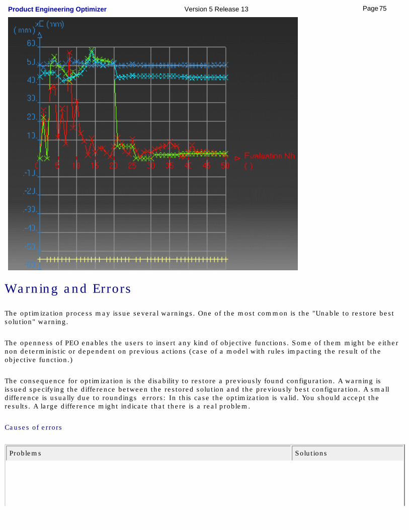
Warning and Errors

The optimization process may issue several warnings. One of the most common is the "Unable to restore best solution" warning.

The openness of PEO enables the users to insert any kind of objective functions. Some of them might be either non deterministic or dependent on previous actions (case of a model with rules impacting the result of the objective function.)

The consequence for optimization is the disability to restore a previously found configuration. A warning is issued specifying the difference between the restored solution and the previously best configuration. A small difference is usually due to roundings errors: In this case the optimization is valid. You should accept the results. A large difference might indicate that there is a real problem.

Causes of errors

Problems Solutions


Models with rules that impact the objective function definition during the optimization process.

f(x)=a x2+1if (x>1) a=1else a = -1

During the optimization process if x takes a value between 1 and 2, the definition of the problem changes.

Check the model.

Models with sketches that can take unreasonable configurations from which they cannot escape.

Always use constraint sketches and use ranges in the optimization.

Analysis models with adapted types of meshing elements that are not adapted (T4 instead of T10.)

Use polynomenial interpolation (T10) instead of linear (T4).


MethodologyFor both algorithms, you can refine the result by removing one or several variables from the list of free parameters and restart the computation.

Algorithms and Objective Function

● In general, the shape of the Objective function is unknown. It is therefore better to begin with a Simulated Annealing and to refine the results with a gradient descent. This approach is slow but works for a larger amount of functions.

● If the properties of the curve are known (continuous, differentiable at all point and with a single optimum), then the gradient can be used straight on. It is usually faster than the Simulated Annealing algorithm.

● If you have to restart the optimization because you are not satisfied with the first result, reduce the ranges on the free parameters and/or reduce the steps.

Algorithms Use

● Approximating a solution with the Simulated Annealing can be quickened by reducing the consecutive bad evaluation stopping criterion to 15 or 20. However, this will increase the risk of a premature convergence to local optimization especially if the optimized problem contains several free parameters.

● For both algorithms, the final results provided can be refined by removing one or several variables and by restarting the optimization.

Ranges and Steps

● It is ALWAYS better to apply ranges to the free parameters (especially for the simulated Annealing). This prevents the geometry from taking unreasonable configurations if the free parameters take too high a value.

● Too big a step makes it useless, but too small a step can prevent fast convergence to a solution. If you are not sure, do not attribute any step but assign ranges.

● Steps are only indicative starting values used by the algorithms: In order to converge toward optimal values both Gradient and SA algorithms need to reduce the steps between consecutive trials. As long as the search makes progress in the same direction (local optimum not detected), the step increases in order to speed up the localization of the local (and global) optimum. As soon as an optimum is located, Gradient and SA do not behave the same way: The gradient algorithm reduces its step in order to reach convergence inside this optimum. The SA makes the step evolve depending on the history of the run according to a complex law. It must be noticed that in no case, the step remains constant.

Constraints

Try to apply constraints with values of the same order of magnitude as the objective function. This will prevent a constraint from being over-considered by the optimization process.


Tips and Tricks

If you encounter a problem with many variables (more than 4) as free parameters:

● do not forget to apply ranges, and

● begin with the gradient algorithm before trying the simulated annealing algorithm.

Gradient

The gradient behaves better with squares or quadratic functions (especially relevant for "Target Values"). Hence the following problem:

Given: volume=x*y*z.

Find, x, y and z such that volume = 1000.

is better solved if the following formula is given to the optimizer:

objective = (volume)2

Chaining algorithms

In most cases the properties of the functions used inside the optimization problem are unknown. In this case, it is recommended to use the global search algorithm (Simulated Annealing). However, since this algorithm can take a long time to reach convergence (especially when there are many free parameters), it could be helpful to use a local search (gradient) for a few iterations before switching to the global search (Simulated Annealing). Eventually, when the global search has converged and that results must be refined, reduce the ranges around the found solution and restart a slow Local Search.

Several constraints

● Some optimization problems can contain a large number of constraints with respect to the number of free parameters. In this case the optimization problem can be over constrained i.e. there is no feasible region (set of free parameter values for which all constraints are satisfied). The Global Search (Simulated Annealing) helps to reduce the constraints values even in this later case. On the other hand it does not guarantee any access to the feasible region even if it exists.

● The evolution of the distances to satisfaction (that can be displayed with the graphs) is useful to

identify constraints that are difficult to satisfy. It is sometime better to deactivate all other constraints in order to identify a potential zone of satisfaction for these constraints only.

Recommendations

Always use well-constrained sketches when they are involved in an optimization. Under constrained sketches can lead to wrong solutions or collapsed geometries (see KwoCirclesSk.CATPart). It is also recommended to

limit the ranges of the free parameters to reasonable values.


Optimal CATIA PLM Usability for Product Engineering Optimizer

When working with ENOVIA V5, the safe save mode ensures that you only create data in CATIA that can be correctly saved in ENOVIA.

ENOVIA V5 offers two different storage modes: Workpackage (Document kept - Publications Exposed) and Explode (Document not kept). Product Engineering Optimizer (PEO) has been configured to work in the Workpackage mode.

Product Engineering Optimizer commands in Enovia V5

Please find below the list of the Product Engineering Optimizer commands along with their accessibility status in Enovia V5.

Note that the restrictions listed below apply only when working at the Product level. They do not apply when working in a Part context.

Commands Accessibility in Enovia V5 (Explode Mode) Comments

Optimize Not available None

Design of Experiments Not available None

Constraint Satisfaction Not available None


Workbench Description This section contains the description of the icons and menus specific to the Product Engineering Optimizer workbench.

The Product Engineering Optimizer workbench is shown below. Click the sensitive areas (toolbars) to access the related documentation.

Product Engineering Optimizer ToolbarConstraint Satisfaction Toolbar


Product Engineering Optimizer Toolbar

The Product Engineering Optimizer toolbar contains the following tools:

See Searching for a Maximum Value, Searching for a Minimum Value.

See Using the Design of Experiments tool.


Constraint Satisfaction ToolbarThe Constraint Satisfaction Toolbar contains the following tool:

See Using the Constraint Satisfaction Function.


Customizing for KnowledgewareThis section describes the ways in which you can customize the Knowledgeware workbenches. See also the Parameters and Measure customizing section.

Knowledge TabLanguage Tab

Report Generation Tab


Knowledge Tab

This task explains how to specify the options when working with Knowledgeware relations, parameters and design tables. Refer to Using Knowledgeware Capabilities for more information.

1. Select the Tools->Options... command. The Options dialog box displays.

2. Select General->Parameters and Measure and click the Knowledge tab. This is what you

can see onscreen:

Parameter Tree View Field


● Check Tools->Options...->General->Parameters and Measure->Knowledge->Parameter Tree View->With value to display the parameter values in the specification tree.

● Check the Tools->Options...->General->Parameters and Measure->Knowledge->Parameter Tree View->With formula to display the formulas constraining the parameter in the specification tree.

Parameter names Field

● Check the Tools->Options...->General->Parameters and Measure->Knowledge->Parameter Names->Surrounded by the symbol' option if you work with non-Latin characters. If this option is unchecked, parameter names should have to be renamed in Latin characters when used in formulas.

Relations update in part context

Before V5R12, Knowledge relations (formulas, rules, checks, design tables, and sets of equations) used to execute as soon as one of their inputs was modified.The user can now choose, when creating the relation, if it will be synchronous (i.e. the evaluation will be launched as soon as one of its parameters is modified) or asynchronous (i.e. the evaluation will be launched when the Part is updated). Each relation can therefore be synchronous or asynchronous.

The 2 following options enable the user to create synchronous or asynchronous relations.

Creation of synchronous relations

Enables the user to create synchronous relations, that is to say relations that will be immediately updated if one of their parameters/inputs is modified. Relations based on parameters are the only one that can be synchronous.

Creation of relations evaluated during the global update

Enables the user to associate the evaluation of asynchronous relations with the global update. The relations can be asynchronous for 2 reasons:

● The user wants the relations to be asynchronous

● The relation contains measures.

● Relations based on parameters: These relations can be synchronous or asynchronous.

● Relations based on geometry: These relations can only be asynchronous.

● Relations based on parameters and on geometry: For the part of the relations containing parameters, the user decides if he wants the update to be synchronous or not. For the other part of the relations, the update occurs when the global update is launched.

Note that the user can also decide if already existing relations are synchronous or asynchronous. To know more, see Controlling Relations Update in the Infrastructure User's Guide.

Design Tables Field


Automatic Synchronization at Load

When loading a model containing user design tables, if the design table files have been modified and the external file data is contained in the model, the design table will be synchronized automatically if this radio button is checked.

Interactive Synchronization at Load

When loading a model containing user design tables whose external source file was deleted, this option enables the user to select a new source file or to save the data contained in the design tables in a new file.

Manual Synchronization

When loading a model containing user design tables, if the design table files have been modified and the external file data is contained in the model, the design table will be synchronized if this radio button is checked. To synchronize both files, right-click the design table in the specification tree and select the DesignTable object->Synchronize command or the Edit->Links command.

Default Mode: Copy Data Into Model

If checked, the data contained in the external source file will be copied into the model.

Default Mode: Do Not Copy Data Into Model

If checked, the data contained in the external source file will not be copied into the model.

3. Click OK when done.


Language Tab

This task explains how to specify the options you may need to check when working with Knowledge browsers.

1. Select the Tools->Options... command. The Options dialog box is displayed.

2. Select General->Parameters and Measure and click the Language tab. This is what you can see

onscreen:

Language Field

This field is to be used when using measures in relations or user functions. Measures are specific

functions to be used in formulas and rules.

The Knowledge Advisor User's Guide provides you with tasks explaining how to use measures. For

how to create and use user functions, see the CATIA Application Architecture documentation.

● Check Tools->Options...->General->Parameters and Measure->Knowledge->Load

extended language libraries and select the packages you want to

load under Packages to load if you want to load a limited number of packages.

This option is particularly useful for the administrator to limit the number of packages used by the user. It is also very useful to improve performances since only the required libraries are loaded.


● When you open a document and some relations are broken, you might need to load

all libraries to solve the error, which may take quite a long time.

● It is strongly recommended to identify the packages you will need and to select them.

● Check Tools->Options...->General->Parameters and Measure->Knowledge

->Load extended language librariesand select All packages to load all the packages

displayed under Packages to load.

Reference Directory For Types field

If you want to reuse the generated type in another CATIA session in the PKT workbench, proceed as

follows:

● save the CATGScript file in the Directory indicated in the Reference Directory for Types field (see

Tools->Options->Parameters and Measure-> Language tab)

● check the Load extended language libraries check box and select the package containing the

type you created.

3. Click OK when done.


Report Generation Tab

This task explains how to customize the reports generated by the Global Check Analysis tool in the Knowledge Advisor and Knowledge Expert workbenches.

You can choose to display a xml or a html report.

Displaying a HTML report

To generate a html report when performing the check analysis, go to Tools->Options->General->Parameters and Measure and select the Report customization tab. Select Html in the Select Report Visualization area.

In this case, only the Check Advisor, the Check expert and the Passed objects options are available in the Report content area. You can specify the output directory containing the generated HTML report in the Select output directory field.

Select Html if you use a Netscape browser.

Displaying a XML report

To display a XML report when performing the check analysis, go to Tools->Options->General->Parameters and Measure and select the Report customization tab. Select Xml in the Select Report Visualization area. The following window opens:


The Report Customization tab is made up of 4 different fields: The Select Input XSL, the Report Content, the Select output directory, and the HTML options fields.

Select Input XSL field

This field enables the user to select the XSL style sheet that will be applied to the generated XML report. The StyleSheet.xsl file is the default XSL file, but you can use your own template.

Report content field

Failed Checks If checked, the generated report will contain information about the failed checks only.

All Checks If checked, the generated report will contain information about all the checks contained in the document.

Check advisorIf checked, the generated report will contain information about all the Knowledge Advisor checks contained in the document.


Parameter information If checked, the generated report will contain information about the

parameters of the Advisor checks.

Check expert If checked, the generated report will contain information about all the Knowledge Expert checks contained in the document.

Passed objects If checked, the generated report will contain information about the objects that passed the Expert checks as well as information about the parameters of these objects (diameter, depth, pitch,...).

Objects information

If checked, the generated report will contain information about all the objects contained in the Expert checks as well as information about the parameters of these objects (diameter, depth, pitch,...).

Select output directory field

This field enables the user to select the output directory containing the generated XML report.

HTML options field

This option is available for Windows only. It enables the user to define if the report will be opened in a CATIA session (in this case, the check box should be checked) or if it will be opened in an Internet Explorer session (in this case, the check box should remain unchecked.)

Note that it is highly recommended not to use this report as a basis for macros or for other applications. It is only provided for information purposes.


Glossary

F

free parameterA parameter which varies according to the optimizer algorithm: These parameters

cannot be driven by a relation (formula, check, rule,...). Other parameters are either

frozen or computed from the free parameter values.

G

gap Equal to the left hand side minus the right hand side (absolute value): |left hand side - right hand side|

Conjugate Gradient A fundamental technique that is often incorporated into various iterative algorithms in

many areas of scientific computing. The Conjugate Gradient method was originally

designed to minimize convex quadratic functions but has been extended to the general

case. A CG algorithm is performing but not very robust.

K

knowledgeware The set of software components dedicated to the creation and manipulation of knowledge-based information. Knowledge-based information consists of rules and other types of relations whereby designers can save their corporate know-how and reuse it later on to drive their design processes.

M

maximization An option of the Optimization process which consists in searching for the maximum value of an objective function.

minimization An option of the Optimization process which consists in searching for the minimum value of an objective function.

O


objective function

A function associated with an optimization problem which determines how good a

solution is. The objective function is a literal feature formula that can be created by

using the formula editor.

optimizationA computational problem in which the aim is to find the best of all possible solutions.

Optimizer An analysis tool which helps users solve an optimization problem.

S

Simulated Annealing A technique used to approximate the solution of very large combinatorial optimization problems. The technique originates from the theory of statistical mechanics and is based upon the analogy between the annealing of solids and solving optimization problems. A Simulated Annealing algorithm is slow but more robust than a CG algorithm.


Index

AAdvanced Tasks

Interpreting Results

Methodology

Tips and Tricks Algorithm

Conjugate Gradient (CG)

Simulated Annealing

Types of Algorithm

Ccommand

Constraint Satisfaction

Design Of Experiments

Optimize

Constraint

Constraint Satisfaction constraint satisfaction

editor

using

using measured parameters in a constraint satisfaction computation

Constraint Satisfaction Editor

Constraint with weight Constraints tab

Activating a constraint

Creating a constraint


DDefining an Optimization

Design of Experiments

Design of Experiments Tool Design of Experiments Window

Prediction tab

Results tab

Settings tab

GGetting Started

Searching for a Target Value with the Gradient Algorithm

Searching for a target value with the Simulated Annealing Algorithm

Global Search Gradient based algorithm

non satisfied constraints

IInterpreting results

Optimization Curves

Result file

Warnings and Errors

LLocal Search

M


Maximization optimization type

Maximum value, searching

measured parameters

Minimization Optimization type

Minimum Value, searching

Ooptimal catia plm usability Optimization Dialog

Constraints tab

Problem tab

The Computations Results tab

Optimization, defining

PProblem tab

Algorithm

Free parameters

Optimization data

Optimization type

Parameter to be optimized


RResult, interpreting

Running a constrained optimization with weights


SSearching for a Maximum Value

Searching for a Minimum Value

UUsing Constraints

Using the Constraint Satisfaction Function


WWeight

Workbench Description


Documents

Product Engineering Optimizer Page 1 Product …bndtechsource.ucoz.com/V5_Online_Docs/Knowledgeware/kwoug2.pdf · Using the Design of Experiments Tool Tips and Tricks Advanced Tasks