Producer Behavior - University of Southern Californiaebayrak/teaching/LECTURES/303/Week 6...The Basics of Production 6.1 Production Functions • Describe how output is made from different

Producer Behavior

6

Introduction 6

Chapter Outline

6.1 The Basics of Production

6.2 Production in the Short Run

6.3 Production in the Long Run

6.4 The Firm’s Cost-Minimization Problem

6.5 Returns to Scale

6.6 Technological Change

6.7 The Firm’s Expansion Path and the Total Cost Curve

6.8 Conclusion

6Introduction

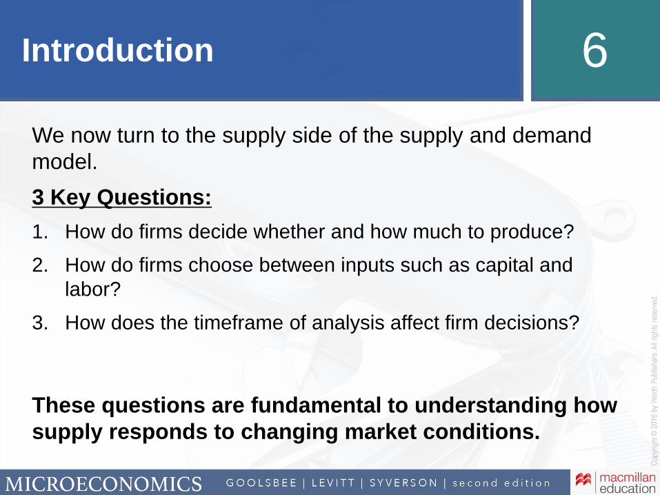
We now turn to the supply side of the supply and demand

model.

3 Key Questions:

1. How do firms decide whether and how much to produce?

2. How do firms choose between inputs such as capital and

labor?

3. How does the timeframe of analysis affect firm decisions?

These questions are fundamental to understanding how

supply responds to changing market conditions.

The Basics of Production 6.1

Production describes the process by which an entity turns raw

inputs into a good or service.

• Final goods are purchased by consumers (e.g., bread).

• Intermediate goods are used as inputs in other production

processes (e.g., wheat used to produce bread).

Start with a production function.

• Mathematical relationship between amount of output and various

combinations of inputs

• Similar to a utility function for consumers, except more tangible


Simplifying Assumptions about Firms’ Production Behavior

1. The firm produces a single good.

2. The firm has already chosen which product to produce,

3. Firms minimize costs associated with every level of production.

• Necessary condition for profit maximization

4. Only two inputs are used in production: capital and labor.

• Capital: buildings, equipment, etc.

• Labor: All human resources


5. In the short run, firms can choose the amount of labor employed,

but capital is assumed to be fixed in total supply.

• Short run: Period of time in which one more inputs used in production

cannot be changed.

• Fixed inputs: Inputs that cannot be changed in the short run.

• Variable inputs: Inputs that can be changed in the short run.

• Long run: Period of time when all inputs in production can be changed.

6. Output increases with inputs.

7. Inputs are characterized by diminishing returns.

• If the amount of capital is held constant, each additional worker

produces less incremental output than the last, and vice versa.

8. The firm can employ unlimited capital and labor at fixed prices, and

9. Capital markets are well functioning (the firm is not budget-

constrained).


Production Functions

• Describe how output is made from different combinations of inputs,

where Q is the quantity of output, K is the quantity of capital used, and L is quantity of labor used.

A common functional form used in economics is referred to as the

Cobb–Douglas production function,

where the quantity of each input, each raised to a power (usually

less than one), are multiplied together.

LKfQ ,

LKQ

Production in the Short Run 6.2

The short run refers to the case in which the level of capital is

fixed, typically expressed as:

First, consider how production changes as we vary the amount of

labor.

Marginal product refers to the additional output that a firm can

produce using an additional unit of an input.

• Similar to marginal utility

• Generally assumed to fall as more of an input is used.

LKfQ ,


The marginal product of labor, MPL , is given as

Consider the production function

where capital is fixed at four units, so plug 4 into the function

Table 6.1 calculates the marginal product of labor for this

production function.

L

QMPL

5.05.0 LKQ

5.05.05.0 24 LLQ



Figure 6.1 A Short-Run Production Function


Table 6.1 and Figure 6.1 reveal the common assumption of

diminishing marginal product associated with production

inputs.

• As a firm employs more of one input, while holding all others

fixed, the marginal product of that input will fall.

.


Returning to the mathematical representation of MPL ,

and using the example production function

As ΔL becomes very small, we use calculus to arrive at the

equation for MPL

This is seen most easily using a graph.

L

LKfLLKf

L

QMPL

,,

5.05.05.0 24 LLQ

L

LLLMPL

5.05.022

5.0

5.0

1, LLdL

LKdfMPL


Figure 6.2 Deriving the Marginal Product of Labor

(a) (b)

MPL

(∆ Q /∆ L )5

1.54.47

4

3.461.0

2.83

2

0.5 MPL

0 0Labor (L) Labor (L)1 2 3 4 5 1 2 3 4 5

Output (Q )Production

function

Slope = 0.45

Slope = 0.5

Slope = 0.58

Slope = 0.71

1Slope = 1 Slope =L0.5


Another important production metric is average product.

• Total output divided by the total amount of an input used

• The average product of labor is given by the equation:

What is the difference between marginal and average product?

‒ The average product uses the total output, while the marginal

product uses the additional output.

L

QAPL

Production in the Long Run 6.3

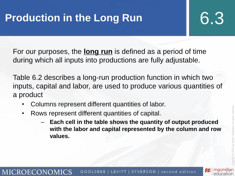
For our purposes, the long run is defined as a period of time

during which all inputs into productions are fully adjustable.

Table 6.2 describes a long-run production function in which two

inputs, capital and labor, are used to produce various quantities of

a product

• Columns represent different quantities of labor.

• Rows represent different quantities of capital.

‒ Each cell in the table shows the quantity of output produced

with the labor and capital represented by the column and row

values.

Production in the Long Run 6.3

The Firm’s Cost-Minimization Problem 6.4

Recall, the third assumption about production behavior:

Firms minimize the cost of production.

Cost minimization refers to the firm’s goal of producing a

specific quantity of output at minimum cost.

• This is an example of a constrained optimization problem.

• The firm will minimize costs subject to a specific amount of output

that must be produced

The cost minimization model requires two concepts, isoquants and

isocost lines


An isoquant is a curve representing combinations of inputs that

allow a firm to make a particular quantity of output

• Similar to indifference curves from consumer theory


Figure 6.3 Isoquants

Capital (K )

4

Output, Q = 4

2

Output, Q = 21

Output, Q = 1

0 Labor (L )1 2 4


An isoquant is a curve representing combinations of inputs that

allow a firm to make a particular quantity of output.

The slope of an isoquant describes how inputs may be substituted to

produce a fixed level of output.

This relationship is referred to as the marginal rate of technical

substitution: The rate at which the firm can trade input X for input Y,

holding output constant (MRTSXY ).


Figure 6.4 The Marginal Rate of Technical Substitution

Capital (K )

A

B

Q =2

Labor (L)

The marginal product ofLabor (MPL) is low relative to the

marginal product of capital (MPK).

The marginal product oflabor (MPL) is high relative to the

marginal product of capital (MPK) .


Mathematically, MRTSLK can be derived from the condition that,

along an isoquant, quantity of output produced is held constant.

Rearranging to find the slope of the isoquant yields the MRTSLK .

Moving down an isoquant, the amount of capital used declines.

• MRTSLK describes the rate at which labor must be substituted for capital to

hold the quantity produced constant.

• As you move down an isoquant, the slope gets smaller, meaning the firm has

less capital and each unit is relatively more productive.

0 KMPLMPQ KL

K

LLKLK

MP

MP

L

KMRTSLMPKMP


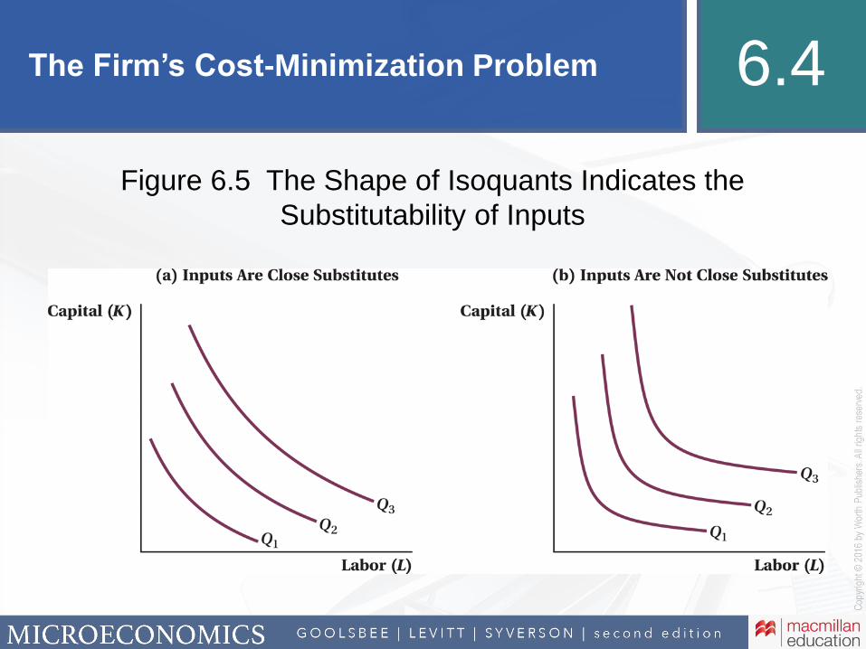
The Curvature of Isoquants: Substitutes and Complements

The shape of an isoquant reveals information about the relationship

between inputs to production

1. Relatively straight isoquants imply that the inputs are relatively substitutable.

• MRTSLK does NOT vary much along the curve.

2. Relatively curved isoquants imply the inputs are relatively complementary.

• MRTSLK varies greatly along the curve.


Figure 6.5 The Shape of Isoquants Indicates the

Substitutability of Inputs



To illustrate, consider extreme cases.

1. When inputs are perfect substitutes, they can be traded off in a

constant ratio in a production process.

• MRTS is constant.


Perfect Substitutes

0 Natural gas (1000 cubic feet)

Consider production of electricity from

either oil or natural gas (Q is kw-hours).

Assume the plant may switch between fuel

sources at a relatively constant rate.

MRTS is constant.

**Numbers are examples1

Q = 1

2

3

4

2 864

Q = 4Q = 3Q = 2

**Numbers are examples

Oil (barrels)



To illustrate, consider extreme cases.

1. When inputs are perfect substitutes, they can be freely substituted

without changing ouptput.

2. When inputs are perfect complements, they must be used in a fixed

ratio as part of a production process.


Perfect Complements

0 Bus drivers

Buses

Consider the provision of bus services.

For a bus to operate, it requires one

driver and one bus.

At point A , two buses are in service.

Adding another driver (point B ) will not

increase the number of buses in

service.

For this, another bus is also needed

(point C ).

1 Q = 1

2

3

1 32

Q = 3

Q = 2A B

C


Isoquant maps show how quantities of inputs are related to output

produced.

An isocost line shows all of the input combinations that yield the same

cost.

• Similar to the budget constraint facing consumers, equation given by

where C is total cost, R is the “rental rate” of capital, and W is the wage rate.

• Rearranging yields capital as a function of the rental rate, wage rate, and

labor.

• Or, graphically

wLrKC

Lr

w

r

CK


Figure 6.7 Isocost Lines

Capital (K )

5

4

3

2

1

C = $50 C = $80 C = $ 100

0 Labor (L )1 2 3 4 5 6 7 8 9 10


Identifying Minimum Cost: Combining Isoquants and Isocost Lines

Remember, the firm’s problem is one of constrained minimization.

• Firms minimize costs subject to a given amount of production.

• Cost minimization is achieved by adjusting the ratio of capital to labor.

‒ Similar to expenditure minimization in Chapter 4

Graphically, cost minimization requires tangency between the isoquant

associated with the chosen level of production, and the lowest cost

isocost line.


Figure 6.10 Cost Minimization

Capital (K )

B (cost-minimizingcombination)

CA

AQ = QCC CB

Labor (L )

CC cannot produce Q. CA can produce Q butis more expensive.


Identifying Minimum Cost: Combining Isoquants and Isocost Lines

Mathematically, tangency occurs where the slope of the isocost line is

equal to the slope of the isoquant, or

What does this condition imply?

• Costs are minimized when the marginal product per dollar spent

is equalized across inputs.

w

MP

r

MP

MP

MP

r

w LK

K

L


Cost Minimizing Condition:

• Costs are minimized when the marginal product per dollar spent

is equalized across inputs.

QUESTION: What if 1. or 2.

1. The marginal product per dollar spent on capital is higher than the

marginal product per dollar spent on labor.

‒ More capital and less labor should be used in production.

2. The marginal product per dollar spent on capital is less than the

marginal product per dollar spent on labor.

‒ More labor and less capital should be used in production.

w

MP

r

MP

MP

MP

r

w LK

K

L

w

MP

r

MP LK w

MP

r

MP LK

Returns to Scale 6.5

Returns to scale refers to the change in output when all inputs are

increased in the same proportion.

Returning to the Cobb–Douglas production function

If we assume , then

• If K = 2 and L = 2, then Q = 2.

What happens if the amount of capital and labor used both double?

Output Doubles!

LKQ

5.0 5.05.0 LKQ

42244 5.05.0 Q


This relationship, whereby production increases proportionally with

inputs, is called Constant Returns to Scale.

• Double inputs Output doubles

• Quadruple inputs Output quadruples

Increasing Returns to Scale: Describes production for which changing

all inputs by the same proportion changes output more than

proportionally.

• Double inputs Output quadruples

Decreasing Returns to Scale: Describes production for which

changing all inputs by the same proportion changes output less than

proportionally.

• Double inputs Output increases by less than double.

• Quadruple inputs Output only doubles.


QUESTION: Why might a firm experience increasing returns to scale?

• Fixed costs (e.g., webpage management, advertising contracts) do not

vary with output.

• Learning by doing may occur, whereby a firm develops more efficient

processes as it expands or produces more output.

Generally, firms should not experience decreasing returns to scale.

• When this phenomenon is observed in data, it often results from not

accounting for all inputs (or attributes).

‒ For instance, second manager may not be as competent as first.

QUESTION: Are there any examples of true decreasing returns?

• Regulatory burden: As firms grow larger, they are often subject to

more regulations.

‒ Compliance costs may be significant.


Figure 6.12 Returns to Scale

(a) (b) (c)Constant Returns to Scale Increasing Returns to Scale Decreasing Returns to Scale

Capital Capital Capital

(K) (K) (K)

4 4 4Q = 4 Q =6 Q =3

2 2 2Q = 2 Q = 2.5 Q = 1.8

1 1 1Q = 1 Q =1 Q =1

0 0 01 2 4 1 2 4 1 2 4

Labor (L) Labor (L) Labor (L)

Note: Labor and capital doubled between isoquants.

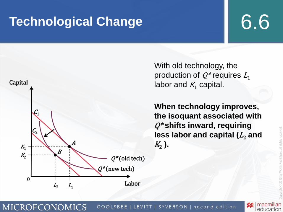
Technological Change 6.6

Examining firm-level production data over time reveals increasing

output, even when input levels are held constant.

• The only way to explain this is by assuming some change to the production

function.

This change is referred to as Total Factor Productivity Growth.

• An improvement in technology that changes the firm’s production function

such that more output is obtained from the same amount of inputs.

Often assumed to enter multiplicatively with production,

where A is the level of total factor productivity.

LKAfQ ,

Technological Change 6.6

0Labor

Capital

With old technology, the

production of Q* requires L1

labor and K1 capital.

When technology improves,

the isoquant associated with

Q* shifts inward, requiring

less labor and capital (L2 and

K2 ).A

BK1

Q* (old tech)

C1

C2

K2

L1

Q* (new tech)

L2

The Firm’s Expansion Path and Total

Cost Curve 6.7

So far, we have only focused on how firms minimize costs, subject to a

fixed quantity of output.

• We can use the cost minimization approach to describe how capital and labor

change as output increases.

An expansion path is a curve that illustrates how the optimal mix of

inputs varies with total output.

This allows construction of the total cost curve, which shows a firm’s

cost of producing particular quantities.

The Firm’s Expansion Path and Total

Cost Curve 6.7

0

Labor (L)

Capital(K)

AB

Q = 20

C = 100 0)Quantity of engines

Total Cost($)

B

A$100

Q = 10

C = 180 C = 300

C

Q = 30

Expansion path

$180

$300

10 20 30

C

Total cost (TC)

Figure 6.15 The Expansion Path and the Total Cost Curve

Conclusion 6.8

This chapter looked closely at how firms make decisions.

• Firms are assumed to minimize costs at every level of production.

• The cost-minimizing combination of inputs occurs where the marginal rate of

technical substitution is equal to the slope of the isocost line.

In Chapter 7 we delve deeper into the different costs facing firms, and

how they change with the level of production.

In-text

figure it out

The short-run production function for a firm that produces

pizza

where Q is the number of pizzas produced per hour, is the

number of ovens (fixed at 3 in the short run), and L is the

number of workers employed.

Answer the following:

a. Write an equation for the short-run production function

with output as a function of labor only,

b. Calculate total output per hour for L = 0,1,2,3,4,5.

c. Calculate the MPL for L=1 to L= 5. Is MPL diminishing?

d. Calculate the APL for the same labor levels as above.

75.025.0

15),( LKLKfQ

In-text

figure it out

a. Capital is fixed in the short run at 3.

Substitute into the production function

b. To calculate total output, simply substitute the

different labor quantities into the production function

above.

3K

75.075.025.0 74.19315 LLQ

Labor Production

L = 0 Q = 19.74(0)0.75 = 0

L = 1 Q = 19.74(1)0.75 = 19.74

L = 2 Q = 19.74(2)0.75 = 33.2

L = 3 Q = 19.74(3)0.75 = 45.01

L = 4 Q = 19.74(4)0.75 = 55.82

L = 5 Q = 19.74(5)0.75 = 66.01

In-text

figure it out

c. The marginal product of labor is the additional amount of

bread produced with one more unit of labor.

Are there diminishing returns to labor? How do you know?

‒ Yes, because as more labor is added the additional output

increases by less than previous unit.

d. Average product is simply total output divided by total

labor used.

Labor Production

L = 0 Q = 19.74(0)0.75 = 0

L = 1 Q = 19.74(1)0.75 = 19.74

L = 2 Q = 19.74(2)0.75 = 33.20

L = 3 Q = 19.74(3)0.75 = 45.01

L = 4 Q = 19.74(4)0.75 = 55.82

L = 5 Q = 19.74(5)0.75 = 66.01

MPL

—

19.74

13.46

11.81

10.81

10.19

APL

—

19.74

16.60

15.00

13.96

13.20

Additional

figure it out

Short-run production function for a local bakery making loaves

of bread

where Q is the number of loaves produced per hour, is the

number of ovens (fixed at 2), and L is the number of workers.


a. Write an equation for the short-run production function

with output as a function of labor only.

b. Calculate total output per hour for L = 0,1,2,3,4,5.

c. Calculate the MPL for L=1 to L=5. Is MPL diminishing?

d. Calculate the APL for the same labor levels above.

25.075.0

20, LKLKfQ

K

Additional

figure it out

a. Capital is fixed in the short run at 2.

Substitute into the production function

b. To calculate total output, simply substitute the different

labor quantities into the production function above.

2K

25.025.075.064.33220 LLQ

Labor Production

L = 0 Q = 33.64(0)0.25 = 0

L = 1 Q = 33.64(1)0.25 = 33.64

L = 2 Q = 33.64(2)0.25 = 40

L = 3 Q = 33.64(3)0.25 = 44.27

L = 4 Q = 33.64(4)0.25 = 47.57

L = 5 Q = 33.64(5)0.25 = 50.30

Additional

figure it out

c. The marginal product of labor is the additional amount of

bread produced with one more unit of labor.

Are there diminishing returns to labor? How do you know?

‒ Yes, because as more labor is added the additional output

increases by less than previous unit.

d. Average product is simply total output divided by total

labor.

Labor Production

L = 0 Q = 33.64(0)0.25 = 0

L = 1 Q = 33.64(1)0.25 = 33.64

L = 2 Q = 33.64(2)0.25 = 40

L = 3 Q = 33.64(3)0.25 = 44.27

L = 4 Q = 33.64(4)0.25 = 47.57

L = 5 Q = 33.64(5)0.25 = 50.30

MPL

—

33.64

6.36

4.27

3.30

2.73

APL

—

33.64

20

14.76

11.89

10.06

In-text

figure it out

Suppose the wage rate is $10 per hour (w = $10/hour) and

the rental rate of capital is $25 per hour (r = $25/hour).


a. Write an equation for the isocost line for a firm.

b. Draw a graph, with labor on the horizontal axis and capital

on the vertical axis, showing the isocost line for C = $800.

‒ Indicate the horizontal and vertical intercepts along

with the slope.

c. Suppose the price of capital falls to $20 per hour. Show

what happens to the C = $800 isocost line, including any

changes in intercepts and the slope.

In-text

figure it out

a. The isocost line always takes the form of 𝑪 = 𝒓𝑲 + 𝒘𝑳.

Plugging in r and w, 𝐶 = 25𝐾 + 10𝐿.

b. With C = $800, the isocost line that will be plotted will be:

800 = 25𝐾 + 10𝐿, the easiest way to plot it is to find the

horizontal and vertical intercepts.

• Horizontal Intercept: The amount of labor the firm could

hire for $800 if it only hired labor (K = 0).

‒$800

𝑤→

$800

$10= 𝟖𝟎 𝒖𝒏𝒊𝒕𝒔

• Vertical Intercept: The amount of capital the firm could hire

for $800 if it only hired capital (L = 0).

‒$800

𝑟→

$800

$25= 𝟑𝟐 𝒖𝒏𝒊𝒕𝒔

Plot these 2 points and draw a line connecting them;

this is the C = $800 isocost line (C1).

In-text

figure it out

Capital (K )

b. The slope of the isocost line is 𝒎 = −𝒘

𝒓= −

𝟏𝟎

𝟐𝟓𝑜𝑟 − 𝟎. 𝟒

Labor (L )80

40

32C1

Slope = − 0.4

c. When r (the price of capital) falls to

$20, only the vertical intercept is

affected.

• If the firm only used capital it could

now employ $800

20= 𝟒𝟎 units.

• The isocost line pivots up and

becomes steeper (C2) with a new

slope

−𝒘

𝒓= −

𝟏𝟎

𝟐𝟎𝑜𝑟 − 𝟎. 𝟓

C2Slope = − 0.5

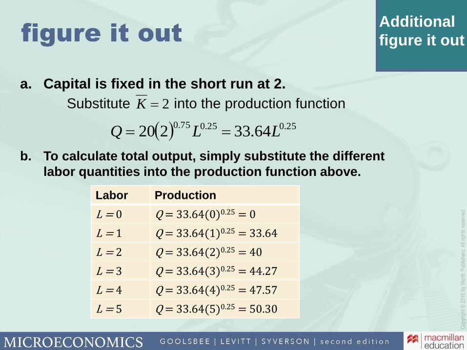
Additional

figure it out

Suppose the wage rate is $10 per hour (w = $10/hour) and

the rental rate of capital is $20 per hour (r = $20/hour).


a. Write an equation for the isocost line for the firm.

b. Draw a graph, with labor on the horizontal axis and capital

on the vertical axis, showing the isocost line for C=$400.

‒ Indicate the horizontal and vertical intercepts along

with the slope.

c. Suppose the price of capital falls to $20 per hour. Show

what happens to the C = $400 isocost line, including any

changes in intercepts and the slope.

Additional

figure it out

a. The isocost line always takes the form of 𝑪 = 𝒓𝑲 + 𝒘𝑳.

Plugging in r and w, 𝐶 = 20𝐾 + 10𝐿

b. With C = $400, the isocost line that will be plotted will be:

400 = 20𝐾 + 10𝐿. The easiest way to plot it is to find the

horizontal and vertical intercepts.

• Horizontal Intercept: The amount of labor the firm could

hire for $400 if it only hired labor (K=0).

‒$400

𝑤→

$400

$10= 𝟒𝟎 𝒖𝒏𝒊𝒕𝒔

• Vertical Intercept: The amount of capital the firm could hire

for $400 if it only hired capital (L= 0)

‒$400

𝑟→

$400

$20= 𝟐𝟎 𝒖𝒏𝒊𝒕𝒔

Plot these 2 points and draw a line connecting them;

this is the C = $800 isocost line (C1).

Additional

figure it out

0Hours of Labor

Hours of Capital

20

Slope = −0.5

20 40

C1

C2

Slope = −1

b. The slope of the isocost line is 𝒎 = −𝒘

𝒓= −

𝟏𝟎

𝟐𝟎𝑜𝑟 − 𝟎. 𝟓

c. When w (the price of labor)

increases to $20 an hour, only the

horizontal intercept is affected.

• If the firm only used labor it could

now employ $400

20= 𝟐𝟎 𝐮𝐧𝐢𝐭𝐬.

• The isocost line pivots in and

becomes steeper (C2) with a new

slope.

−𝒘

𝒓= −

𝟐𝟎

𝟐𝟎𝑜𝑟 − 𝟏

In-text

figure it out

A firm is employing 100 workers (w = $15/hour) and 50 units

of capital (r = $30/hour). At these levels, the marginal product

of labor (MPL) is 45 and the marginal product of capital (MPK)

is 60.


a. Is this firm minimizing costs?

b. If not, what changes should they make?

c. How does the answer to (2) depend on the timeframe of

analysis?

In-text

figure it out

a. Cost minimization occurs when

For this firm, we have

Since these two ratios are not equal, the firm is not minimizing costs.

b. As𝑴𝑷𝑳

𝒘>

𝑴𝑷𝑲

𝒓, changing the mix of capital and labor can lead to a

lower cost of producing the same quantity of output.

• $1 spent on labor yields a greater marginal product (i.e. more output) than $1

spent on capital.

• The wages to labor and capital are fixed, so to equate these two, the quantity

of labor employed must rise and/or the quantity of capital employed must fall.

c. Generally, the short run implies that only the amount of labor employed can be

altered.

/ /L KMP w MP r

w

MP

r

MP LK

230

60

r

MPK

315

45

w

MPL

Additional

figure it out

A firm is employing 25 workers (w = $10/hour) and 5 units of

capital (r = $20/hour). At these levels, the marginal product of

labor (MPL) is 25 and the marginal product of capital (MPK) is

30.


a. Is this firm minimizing costs?

b. If not, what changes should they make?

c. How does the answer to (2) depend on the timeframe of

analysis?

Additional

figure it out

a. Cost minimization occurs when

For this firm, we have

Since these two ratios are not equal, the firm is not minimizing costs.

b. As 𝑴𝑷𝑳

𝒘>

𝑴𝑷𝑲

𝒓, changing the mix of capital and labor can lead to a lower

cost of producing the same quantity of output.

• $1 spent on labor yields a greater marginal product (i.e. more output) than $1

spent on capital.

• The wages to labor and capital are fixed, so to equate these two, the quantity

of labor employed must rise and/or the quantity of capital employed must fall.

c. Generally, the short run implies that only the amount of labor

employed can be altered.

/ /L KMP w MP r

w

MP

r

MP LK

5.120

30

r

MPK

5.210

25

w

MPL

In-text

figure it out

For each of the following production functions, determine if

they exhibit constant, decreasing, or increasing returns to

scale.

a.

b.

c.

LKQ 152

)4,3min( LKQ

4.05.015 LKQ

In-text

figure it out

The simplest way to determine returns to scale is to plug

in values for labor and capital, calculate output, then

double the inputs and calculate output again.

a. Consider K = L = 1

Now, double the inputs (K and L now = 2).

Since output doubled when inputs doubled, we have constant

returns to scale.

17152152 LKQ

3421522152 LKQ

In-text

figure it out

b. Consider K = L = 1 again.


Once again, we have constant returns to scale.

c. K = L = 1

Now, double the inputs (K and L now =2).

Since the new output is less than twice the old output, we have

decreasing returns to scale.

34 ,3min LKQ

624 ,23min Q

1515 4.05.0 LKQ

99.272215 4.05.0 Q

Additional

figure it out

For each of the following production functions, determine if

they exhibit constant, decreasing, or increasing returns to

scale.

a.

b.

c.

LKQ 53

LKQ 5 ,6min3.06.018 LKQ

Additional

figure it out

The simplest way to determine returns to scale is to plug

in values for labor and capital, calculate output, then

double the inputs and calculate output again.

a. Consider K = L = 2.


Since output doubled when inputs doubled, we have constant

returns to scale.

1610653 LKQ

32454353 LKQ

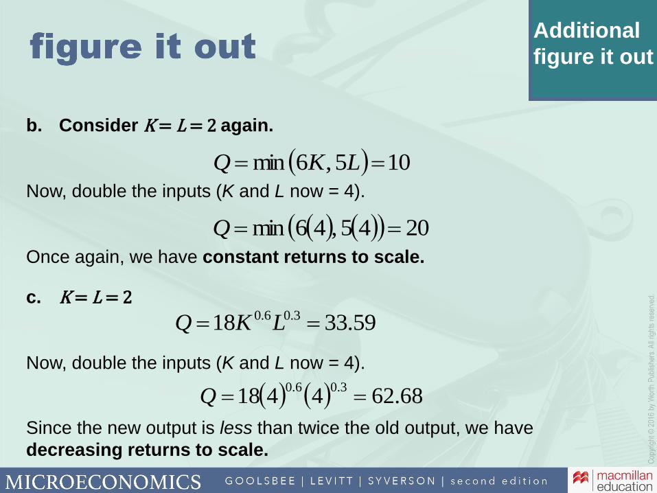
Additional

figure it out

b. Consider K = L = 2 again.


Once again, we have constant returns to scale.

c. K = L = 2


Since the new output is less than twice the old output, we have

decreasing returns to scale.

105 ,6min LKQ

2045 ,46min Q

59.3318 3.06.0 LKQ

68.6244183.06.0Q

Documents

Producer Behavior - University of Southern Californiaebayrak/teaching/LECTURES/303/Week 6...The Basics of Production 6.1 Production Functions • Describe how output is made from different