Earth Planets Space, 60, 529–537, 2008

Procrustean solution of the 9-parameter transformation problem

J. L. Awange, K.-H. Bae, and S. J. Claessens

Western Australian Centre for Geodesy & The Institute for Geoscience Research, Curtin University of Technology,GPO Box U1987, Perth, WA 6845, Australia

(Received May 10, 2007; Revised February 8, 2008; Accepted February 9, 2008; Online published July 4, 2008)

The Procrustean “matching bed” is employed here to provide direct solution to the 9-parameter transformationproblem inherent in geodesy, navigation, computer vision and medicine. By computing the centre of masscoordinates of two given systems; scale, translation and rotation parameters are optimised using the Frobeniusnorm. To demonstrate the Procrustean approach, three simulated and one real geodetic network are tested. In thefirst case, a minimum three point network is simulated. The second and third cases consider the over-determinedeight- and 1 million-point networks, respectively. The 1 million point simulated network mimics the case of anair-borne laser scanner, which does not require an isotropic scale since scale varies in the X , Y , Z directions. Areal network is then finally considered by computing both the 7 and 9 transformation parameters, which transformthe Australian Geodetic Datum (AGD 84) to Geocentric Datum Australia (GDA 94). The results indicate theeffectiveness of the Procrustean method in solving the 9-parameter transformation problem; with case 1 givingthe square root of the trace of the error matrix and the mean square root of the trace of the error matrix as 0.039 mand 0.013 m, respectively. Case 2 gives 1.13×10−12 m and 2.31×10−13 m, while case 3 gives 2.00×10−4 m and1.20 × 10−5 m, which is acceptable from a laser scanning point of view since the acceptable error limit is below1 m. For the real network, the values 6.789 m and 0.432 m were obtained for the 9-parameter transformationproblem and 6.867 m and 0.438 m for the 7-parameter transformation problem, a marginal improvement by1.14%.Key words: Procrustes, 9-parameter transformation, least squares solution, Frobenius, singular value decompo-sition (SVD).

1. IntroductionThe 9-parameter affine transformation is defined as the

problem of determining three scale parameters in the X , Y ,Z directions (diag{S} ∈ R

3×3), three rotation parameters(R ∈ R

3×3) and three translation parameters (T ∈ R3×1).

It is an extension of the 7-parameter transformation prob-lem (Bursa, 1962; Wolf, 1963), with the scales determinedalong the three axes X , Y , Z instead of the usual scalarvalue.

Suppose that the scale is not uniform within two or moreconurations of points such that they vary within given di-mensions. This is typical in the 9-parameter transformationproblem. In this case, transforming the coordinates of oneconfiguration to those of another will require, in additionto rotation and translation elements, the solution of scaleparameters s1, s2, s3 corresponding to the 3 (X, Y, Z ) di-mensions. The 9-parameter transformation is used in thefields of geodesy (Antonopoulos, 2003; Watson, 2006),navigation (Forsberg, 1991), medicine (Piperakis and Ku-mazawa, 2001; Pfefferbaum et al., 2006; Sun et al., 2007),computer image analysis (Ashburner and Friston, 1997)and surface modelling (Niederoest, 2003; Gruen and Akca,2005). Furthermore, the 9-parameter transformation is in-cluded in several geodetic coordinate transformation pack-

Copyright c© The Society of Geomagnetism and Earth, Planetary and Space Sci-ences (SGEPSS); The Seismological Society of Japan; The Volcanological Societyof Japan; The Geodetic Society of Japan; The Japanese Society for Planetary Sci-ences; TERRAPUB.

ages, which use iterative approaches requiring initial start-ing values (e.g., Mathes, 2002; Frohlich and Broker, 2003).They can also find use in correcting for distortion where therotation and translation elements have been determined ex-clusive of scales, e.g., in Featherstone and Vanıcek (1999).

The solution of the transformation parameters has at-tracted a wide range of research, e.g., Spath (2004), who ap-plies a numerical minimization technique, Papp and Szucs(2005), who apply a linearized least-squares method andWatson (2006), who applies the Gauss-Newton method.The Multidimensional Scaling (MDS) approach of Pro-crustes has also been widely used in recent studies.

Borg and Groenen (1997) define Multidimensional Scal-ing as a method that represents measurements of similarity(dissimilarity) of data as distances among points in a geo-metric space of low dimensionality. Let us consider a dataset to consist of tests and that a correlation of tests is re-quired. MDS can be used to represent these data in a planesuch that their correlation can be studied. The closer to-gether the points are (i.e., the shorter the distance betweenthe points) the more correlated they are. MDS thus givesthe advantage of graphical visualization of hidden adherentproperties between objects. Procrustes is a procedure usedin MDS to realise its goals. It is a tool of MDS concernedwith fitting one configuration to another as close as possible.Put in matrix form, the Procrustes problem asks how closelya matrix A can be approximated by a second, given, matrixB which is multiplied by an orthogonal matrix T. The ad-

529

530 J. L. AWANGE et al.: PROCRUSTEAN 9-PARAMETER TRANSFORMATION

vantage it enjoys over the conventional methods is that itdoes not rely on approximate starting values, and that it isnot iterative in nature. It offers a direct solution to nonlineartransformation equations (see, e.g., Awange and Grafarend,2005).

In the Procrustean method, the rotation matrix is first es-timated using singular value decomposition (SVD) of thetwo sets of coordinates, and then the translation and scalefactors are estimated using these estimated rotation param-eters. Therefore, the rotation parameters are independent ofthe number of scale factors in the transformation.

Whereas the Procrustean approach has successfully beenapplied to solve the 7-parameter datum transformation (alsoknown as the Helmert transformation) problem (e.g., Gra-farend and Awange, 2000, 2003; Awange and Grafarend,2005; Umeyama, 1991; Beinat and Crosilla, 2001, 2002),its application to solve the 9-parameter transformationproblem has not been attempted. This has been due to thevery nature of the Procrustean approach, which is designedto give isotropic dilation, three rotation and three translationparameters (Cox and Cox, 1994), whereas the 9-parametertransformation requires the solution of three scale parame-ters. In solving the 9-parameter transformation problem forexample, Watson (2006) circumvents the limitation of theProcrustean solution by solving rotational elements usingGauss-Newton iteration.

Lingoes and Borg (1978) proposed the PINDIS (Pro-crustean Individual Differences Scaling) approach to scaleindividual similarities according to the dimensional saliencemodel. The PINDIS approach obtains the estimates by min-imizing the trace of the sum of squares of residuals, wheresuch residuals are obtained by subtracting parameters in agiven configurations from the centroid values. Due to fail-ure of achieving an analytical solution, the PINDIS algo-rithm reverts to iterative procedures (see, e.g., Comman-deur, 1991, p. 8). The shortcomings of PINDIS have beenpointed out in Commandeur (1991) who goes a step fur-ther to provide a general solution for scaling factors. Com-mandeur (ibid, p. 34) achieves the general solution of scalefactors through the use of a constraint such that the sumof squares about the origin of the scaled configurations re-mains equal to the sum of squares of the original configura-tions centered on the origin.

The common feature between the Lingoes and Borg(1978) and Commandeur (1991) approaches is that thescales are assumed to be uniform in a given configurationand solved throughout for the total number of configura-tions. Assuming x j to be a column vector containing thecoordinates of points j = 1, . . . , n in m-dimensional space,the scale is defined as s j . For two configurations j = 1, 2in m = 3 dimensions, these procedures will be solving fors1 and s2 scales, i.e., one scale parameter for each configu-ration. This is distinctly different from 9-parameter trans-formation studied here, which seeks to solve one scale pa-rameter for each dimension, thus three in total, while thenumber of configurations is restricted to two.

This study attempts to provide a complete Procrusteansolution of the 9-parameter transformation problem by solv-ing the 3 scale parameters (s1, s2, s3), 3 rotation and 3translation parameters. The physical meaning of these

scale parameters can be interpreted as follows: given three-dimensional coordinates in two systems, the rigid transfor-mation from one system to another will involve rotatingabout and translating along the X -, Y -, and Z -axis. In somesystems such as in photogrammetry and laser scanning,some discrepancies exists along these axes which can beovercome by applying different scales to each of the axes,hence the need for scale parameters. In addition, applyingdifferent scale parameters in geodetic coordinate transfor-mations can better account for systematic observation errorsor processes such as solid Earth deformation.

The advantages of using Procrustean transformation inthe case of the 7-parameter transformation are its direct ap-proach, which alleviates the need for linearization, initialstarting values, and iterations inherent in least-squares so-lution (LSS), and also its simplicity compared to other ap-proaches (e.g., Awange and Grafarend, 2005). Its successis mainly due to the fact that it is designed to give isotropicdilation, rotation and translation of rigid bodies. For a uni-form scale therefore, as is the case in the 7-parameter trans-formation, the application is straightforward.

For the 9-parameter affine transformation, there is, how-ever, the requirement to determine three scale parametersinstead of one, thereby presenting a challenge to the Pro-crustean method designed for one scale factor. The presentstudy presents the first attempt to apply Procrustes to solvethe 9-parameter transformation problem. The approach re-duces the coordinates of the two systems into their centre ofmass, optimizes the scale in the sense of LSS with the rota-tion matrix determined by means of singular value decom-position (SVD) also known as Eckert-Young decomposition(Eckert and Young, 1936).

The study is organized as follows: In Section 2, the9-parameter transformation problem is introduced and itsProcrustean solution is presented in Section 3. Section 4considers test examples, while Section 5 summarizes theresults.

2. Definition of the ProblemLet us consider two coordinate configurations A ∈ R

n×m

and B ∈ Rn×m consisting of n points in an m-dimensional

Euclidean space. The dataset in A and B spaces are ex-pressed by

A =

x1 y1 z1

x2 y2 z2

· · ·xn yn zn

, B =

X1 Y1 Z1

X2 Y2 Z2

· · ·Xn Yn Zn

. (1)

The 7-parameter similarity or Helmert transformation prob-lem is defined by

A = BRs + vTT , (2)

where R ∈ R3×3 is an orthonormal rotation matrix satis-

fying the orthogonality condition RT R = I3. The rotationmatrix is parameterized by either Cardan or Euler rotationangles (Awange and Grafarend, 2005, pp. 262–263) and therotation convention of Soler (1998) is commonly used to de-fine the direction of the rotations. s ∈ R is the scale factoralso known as dilation, T ∈ R

3×1 is the translation vector

J. L. AWANGE et al.: PROCRUSTEAN 9-PARAMETER TRANSFORMATION 531

and v is a vector of ones with length n. The 7-parametertransformation problem is now solved by determining the 7transformation parameters, i.e., scale s ∈ R, 3 rotation ele-ments of R ∈ R

3×3, and 3 translation parameters T ∈ R3×1.

Various approaches for solving the 7-parameter transforma-tion problem have been discussed, e.g., in Awange and Gra-farend (2005).

The 9-parameter transformation problem, on the otherhand, concerns itself with the solution of

A = BRS + vTT , (3)

where the scalar parameter s ∈ R in Eq. (2) has beensubstituted with a diagonal matrix S ∈ R

3×3 given by

S = sx

sy

sz

, (4)

with sx , sy , sz being the X , Y , Z scales in the directions, re-spectively. As opposed to the solution of Eq. (2), Eq. (3) en-tails the determination of nine parameters, i.e., three scalesS ∈ R

3×3, three rotations elements of R ∈ R3×3 and three

translation parameters T ∈ R3×1.

3. Solution of the 9 Transformation ParametersFrom Eqs. (1) and (3), let bi = [Xi Yi Zi ] and ai =

[xi yi zi ]. In order to obtain optimum 9-transformationparameters, scale diag(S) ∈ R

3×3, rotation R ∈ R3×3

and translation T ∈ R3×1 are determined, such that the

Frobenius norm is minimum, i.e., the sum of square ofdistances between points in A ∈ R

n×m and B ∈ Rn×m

coordinate systems

D2 =n∑

i=1

(ai − bi RS − T)T (ai − bi RS − T). (5)

Optimal translation vector estimation:Considering a0 and b0 to be the center of mass (centroid)

of the two coordinate configurations A and B derived from

a0 = 1

n

n∑i=1

ai , b0 = 1

n

n∑i=1

bi . (6)

The error metric (Eq. (5)), in the centralised coordinate isgiven by

D2 =n∑

i=1

[(ai − a0) − (bi − b0)RS + a0 − b0RS − T]T

[(ai − a0) − (bi − b0)RS + a0 − b0RS − T], (7)

which on expanding leads to (Cox and Cox, 1994)

D2 =n∑

i=1

[(ai − a0) − (bi − b0)RS]T

[(ai − a0) − (bi − b0)RS]

+n(a0 − b0RS − T)T (a0 − b0RS − T). (8)

A close examination of Eq. (8) reveals that the last termis non-negative and contains the translational element T ∈

R3×1. D2 can attain a minimum if the last term in Eq. (8)

equals zero, i.e., if

T = a0 − b0RS. (9)

Alternatively, from Eq. (3), T ∈ R3×1 can also be obtained

by taking the mean of the translations, i.e.,

Ti = 1

n

n∑i=1

(ai − bi RS) = 1

n

n∑i=1

ai − 1

n

n∑i=1

bi RS, (10)

which together with Eq. (6) leads to the translation elementsin Eq. (9).Optimal scale parameter estimation:

Assuming the centroids a0 = b0 = 0, then from Eq. (3),

A = BRS. (11)

Let f be the error function incurred in rotating the system Band scaling it to match A. Thus

f = (A − BRS)T (A − BRS), (12)

where f is a 3 × 3 matrix. As in the translation estimation,the Frobenius norm is applied to the error function by min-imizing the distances between two corresponding points,and this norm is minimized (cf. Fitzpatrick and West, 2001)

‖f‖2F = tr{(A − BRS)T (A − BRS)} := min (13)

The optimal least squares solution of S ∈ R3×3 can be found

by minimising the ‖f‖2F such that

∂‖f‖2F

∂s j= 0, necessary condition

∂2‖f‖2F

∂s2j

≥ 0, sufficient condition

j ∈ {1, 2, 3},

(14)where s1, s2, and s3 are the scale parameters in the directionof X , Y and Z , respectively. Since S is a diagonal matrix,and thereby symmetric, the following relations hold (Gra-farend and Schaffrin, 1993, p. 443)

∂ tr(SRT BT A)

∂S= ∂ tr(AT BRS)

∂S= RT BT A

∂ tr(SRT BT BRS)

∂S= 2RT BT BRS

(15)

Then, the first and second derivatives of ‖f‖2F with respect

to S ∈ R3×3 in Eq. (12) are

∂‖f‖2F

∂S= −2RT BT A + 2RT BT BRS

∂2‖f‖2F

∂S2= 2RT BT BR

(16)

Note that the sufficient condition in Eq. (14) is observed,since the second derivative in Eq. (16) is a quadratic form.

By setting ∂‖f‖2F

∂S = 0, the optimal least-squares solution forS can be found

S = (RT BT BR)−1RT BT A. (17)

532 J. L. AWANGE et al.: PROCRUSTEAN 9-PARAMETER TRANSFORMATION

However, the solution of Eq. (17) will generally result ina full S matrix instead of the desired diagonal matrix. Toavoid this situation, such that the off-diagonal elements ofS in Eq. (14) are zero, Eq. (16) needs to be evaluated termby term. Introducing the following term-wise notation of A,B and R

A =

a11 a12 a13

a21 a22 a23

· · ·an1 an2 an3

, B =

b11 b12 b13

b21 b22 b23

· · ·bn1 bn2 bn3

,

R = r11 r12 r13

r21 r22 r23

rn1 rn2 rn3

, (18)

it is deduced (see Appendix) that the elements of ∂‖f‖2F

∂S aregiven by

{∂‖f‖2

F

∂S

}i j

= −2n∑

l=1

(3∑

k=1

blkrki

)al j

+ 2s j

n∑l=1

(3∑

k=1

blkrki

) (3∑

k=1

blkrk j

). (19)

Setting the diagonal elements (i = j) to zero in Eq. (19)gives the solution for the scale parameters s j

{∂‖f‖2

F

∂S

}j j

= 0 ⇔ s j =

n∑l=1

(3∑

k=1

blkrk j

)al j

n∑l=1

(3∑

k=1

blkrk j

)2 ,

j ∈ {1, 2, 3}. (20)

Note that this solution can also be found by expressingtr{(A − BRS)T (A − BRS)} in term-wise notation, and thendifferentiating the result with respect to s j .

In deriving Eq. (20), we made use of the assumptiona0 = b0 = 0 which may not always hold due to poor net-work geometry. In order to take into consideration residualerrors arising due to the assumption a0 = b0 = 0, the scaleis rigorously solved as follows: Let the error in scale asso-ciated with the assumption a0 = b0 = 0 be dS. A linearexpression in S is then written as

S = S0 + dS, (21)

where S0 is given by Eq. (20). This is then solved via leastsquares as

dS = diag((RT BT BR)−1RT BT w), (22)

andw = A − BRS0 − v(a0 − b0RS0), (23)

where the diagonal operator, diag, means that a matrix is‘diagonalized’ by setting the non-diagonal elements to zeroand dS is still a 3 × 3 matrix after this operation. Note thatEq. (20) is influenced by the assumption a0 = b0 = 0 andthus few iterations based on Eqs. (21)–(23) are generallyrequired as shown in Section 4.

Fig. 1. Procrustean 9-parameter transformation algorithm.

Optimal rotation matrix estimation:In Eqs. (9) and (17), the rotation matrix is required for

solving the scale and translation elements. Here, we illus-trate how it can be obtained from the partial orthogonal Pro-crustes method which makes use of only the coordinatesin two systems and does not require linearization, iterationor the knowledge of approximate starting values. Considerthe transformation problem about the origin a0 = b0 = 0.Since the solution of R ∈ R

3×3 can be obtained from coor-dinates independent of the scale and translation parameters(Grafarend and Awange, 2003; Watson, 2006), Eq. (3) isexpressed as

A = BR, (24)

subject to the quadratic constraint and the orthogonalitycondition of the rotation matrix R (Grafarend and Awange,2003)

RT R = I3 (25)

The 3 × 3 orthonormal matrix R ∈ R3×3 is a least-squares

solution of Eq. (24) with the condition in Eq. (25), if andonly if, it fulfils the system of nonlinear normal equation

BT BR + R� = BT A, (26)

where � is a symmetric 3×3 matrix of Lagrange multipliers(Grafarend and Awange, 2000).

If the singular value decomposition of BT A is expressedas

U�VT = BT A, (27)

then a solution of the system of nonlinear normal equationsis

R = UVT (28)

which is unique if the rank of BT A ∈ Rm×m is equal

or greater than 3 (Grafarend and Awange, 2000). Other

J. L. AWANGE et al.: PROCRUSTEAN 9-PARAMETER TRANSFORMATION 533

Table 1. True and estimated transformation parameters for simulated 3 points network. Rota, Rotb and Rotc are the rotation angles around the x , y andz axes.

True value Estimated value Difference

sx 0.99998 0.99998 4.608314 × 10−11

sy 0.99994 0.99994 4.608192 × 10−11

sz 0.99995 0.99995 1.221245 × 10−15

Tx (m) 100.0 100.019010 −0.019010

Ty (m) 20.0 19.975360 0.024640

Tz (m) 0.0 1.136868 × 10−13 −1.136868 × 10−13

Rota (‘’) 1.0 0.999971 2.880136 × 10−5

Rotb (‘’) 3.0 3.000010 −9.600299 × 10−6

Rotc (‘’) 0.5 2.480232 −1.980232

Fig. 2. Two simulated three dimensional 3-points networks.

methods of obtaining Eq. (28) have been presented, e.g.,in Awange and Grafarend (2005). The Procrustean 9-parameter transformation algorithm is presented in Fig. 1.

4. Test ResultsIn this section, the proposed Procrustean 9-parameter

transformation is tested using simulated datasets and a realnetwork. Regarding the number of points in a test network,we utilize the minimum required number, i.e., 3, to a largenumber of points, 1 million as can be the case of the pointcloud registration of air-borne laser scanner datasets.

The simulation adopts a “forward-backward” strategy,where we start with some arbitrary coordinates of A andvalues of the 9 transformation parameters. These are thenused in the “forward step” to simulate the coordinates ofconfiguration B. In the “backward step”, we use the sim-ulated coordinates of B and those of A to derive the trans-formation parameters using the Procrustean 9-parameter al-gorithm. A comparison is then made between the ‘forward’and ‘backward’ transformation parameters. The computedtransformation parameters from the “backward step” areused to transform the coordinates of B into A and the er-rors are analysed using two error measures errE and MerrE,which are defined as (e.g., Grafarend and Awange, 2003)

errE =√

tr(ET E) (29)

and

MerrE =√

tr(ET E)

3n, (30)

where E is the error matrix

E = A − BRS − v(a0 − b0RS). (31)

The error matrix norm errE is thus the square root of thesum of the squared coordinate differences before and aftertransformation. This error measure is generally larger forcases with a larger number of points. The mean error ma-trix norm MerrE divides the sum of the squares by the to-tal number of coordinates to obtain the root-mean-squares(RMS) of the coordinate differences, and is more suitableto compare cases with different numbers of points.Case 1 (simulated 3 points network)

In this case, two networks consisting of 3 commonpoints, which is the minimum required numbers of pointsfor Procrustean 9-parameter transformation, are utilized asshown in Fig. 2. This example is important for a case whereonly the bare minimum number of points are available inboth systems as is often the case in Photogrammetry. Thetransformation parameters between A and B, i.e., 3-scalefactors, 3-translational and 3-rotational parameters are com-puted using the Procrustean 9-parameter algorithm and arepresented in Table 1. The error measures errE and MerrE

534 J. L. AWANGE et al.: PROCRUSTEAN 9-PARAMETER TRANSFORMATION

Table 2. True and estimated transformation parameters for simulated 8 point network.

True value Estimated value Difference

sx 0.99998 0.99998 1.928983 × 10−8

sy 0.99994 0.99994 4.178106 × 10−9

sz 0.99995 0.99995 −6.129651 × 10−8

Tx (m) 100.0 100.000000 −1.421086 × 10−14

Ty (m) 20.0 20.000000 8.526513 × 10−14

Tz (m) 0.0 −8.526513 × 10−14 8.526513 × 10−14

Rota (‘’) 1.0 0.993931 0.006069

Rotb (‘’) 3.0 3.013453 −0.013453

Rotc (‘’) 0.5 0.487267 0.012733

Fig. 3. Two simulated three dimensional 8-points networks.

computed using (Eq. (29)) and (Eq. (30)) are 0.0392 m and0.0131 m, respectively. The difference between the truetransformation parameters and those computed using Pro-crustean algorithm are presented in Table 1. The differencesare close to zero for scale and rotation elements, exceptfor the Z -axis rotation. The Z -axis rotation error is muchlarger than the other direction errors since the range of theZ -direction data is much smaller than that of either X - or Y -axis dataset in Case 1, which causes the difference in Rot(c)to be slightly larger. The differences found in Tx and Ty areindeed related to this. This is also attributed to the fact thatwe are dealing with the minimum case. As the number ofstations increase, e.g., in Cases 2 and 3, the effect becomesmuch less. No iteration for scale was required for this casein order to obtain the final MerrE value of 0.013064 m sincethe network geometry is good.Case 2 (8-points network)

Next, two networks with 8 points shown in Fig. 3 areutilized. This example depicts a localized surveying sit-uation where a couple of points common in both systemsare available. The error measures errE and MerrE are com-puted as 1.132 × 10−12 m and 2.311 × 10−13 m. The dif-ferences between the true and estimated values of the 9-transformation parameters are presented in Table 2 are closeto zero. Compared to case 1, the differences in the sim-ulated 8-points networks are much smaller due to a largenumber of redundant points and a better network configura-tion compared to the minimal case of 3 points highlightingthe well known fact of utilizing as many points as possible.

For this simulated network, no iteration was required simi-lar to the simulated 3-point network to obtain a MerrE valueof 2.311370 × 10−13 m.Case 3 (1 million points network)

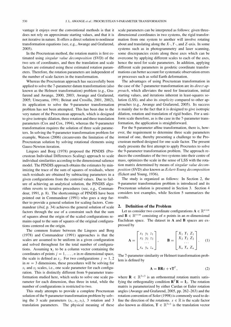
For this case, two networks of one million commonpoints are simulated. This case can be regarded as an ex-ample of an air-borne laser scanner point clouds situationin which the proposed Procrustean algorithm for solving 9-parameter transformation parameters can be useful since itis likely to have anisotropic scale factors. The error mea-sures errE and MerrE are computed as 3.83 × 10−4 m and2.208 × 10−7 m. The true and estimated transformation pa-rameters are given in Table 3. From the plot of errE andMerrE vs iteration presented in Fig. 4, four iterations aresufficient for this case.Case 4 (82-common known stations in both AGD 84 andGDA 94)

Finally, a real network dataset based on 82 stations com-mon in both AGD 84 and GDA 94 (Fig. 5) are used tocompute the transformation parameters for Western Aus-tralia. The AGD is defined by the ellipsoid with a semi-major axis of 6378160 m and a flattening of 0.00335289while the GDA is defined by an ellipsoid of semi-majoraxis 6378137 m and a flattening of 0.00335281 (Kinneenand Featherstone, 2004). Both 7- and 9-transformationparameters are computed using the general 7-parameterProcrustean algorithm and the proposed 9-parameter Pro-crustean algorithms respectively. The resultant error mea-sures errE and MerrE are then compared. For the 7-

J. L. AWANGE et al.: PROCRUSTEAN 9-PARAMETER TRANSFORMATION 535

Table 3. True and estimated transformation parameters for the simulated network with 1 million points.

True values Estimated values Difference

sx 0.99998 0.99998 7.193998 × 10−10

sy 0.99994 0.99994 −7.097811 × 10−11

sz 0.99995 0.99995 −1.064053 × 10−9

Tx (m) 400.0 399.999999 5.075449 × 10−7

Ty (m) 300.0 300.000000 −1.495559 × 10−7

Tz (m) 5.0 5.000000 4.753149 × 10−7

Rota (‘’) 1.0 1.000072 −7.164506 × 10−5

Rotb (‘’) 3.0 3.000320 −3.19516 × 10−4

Rotc (‘’) 0.5 0.500084 −8.387693 × 10−5

Error X (m) Error Y (m) Error Z (m)

Min. −6.5690 × 10−7 −5.9980 × 10−7 −3.6550 × 10−7

Max. 6.5630 × 10−7 6.0090 × 10−7 3.6430 × 10−7

Average −7.1977 × 10−12 4.6118 × 10−12 −1.1743 × 10−11

Fig. 4. Error versus iteration for the simulated network with 1 millionpoints.

Fig. 5. Locations of the 82 stations in WA, Australia (AGD84 andGDA94).

Table 4. Error metrics from 9 and 7 parameters transformation with 82stations in WA, Australia (AGD84 and GDA94).

9-parameters 7-parameters Improvement (%)

errE 6.788556 6.866908 1.14

MerrE 0.432822 0.437818 1.14

Table 5. Estimated transformation parameters between 82 stations in WA,Australia (AGD84 and GDA94) using 9- and 7-parameter transforma-tion methods.

Estimated values Estimated values

(9-parameters) (7-parameters)

s 1.00000368981

sx 1.00000396085

sy 1.00000355062

sz 1.00000345982

Tx (m) −115.061896 −115.837707

Ty (m) −47.697857 −48.373207

Tz (m) 144.095506 144.759551

Rota (‘’) 0.119711 0.119712

Rotb (‘’) 0.383988 0.383988

Rotc (‘’) 0.370396 0.370396

parameter solution, the error measures errE and MerrE are6.867 m and 0.438 m, while the 9-parameter solution gives6.789 m and 0.433 m which is a marginal 1.4% improve-ment on the results obtained with the 7-parameter transfor-mation (see Table 4). The estimated transformation param-eters are given in Table 5. The Error plots of each stationfor 82 stations in WA are presented in Fig. 6 while the plotof errE and MerrE versus iteration is presented in Fig. 7,which demonstrates that 4 iterations are required to obtaina precise scale matrix.

5. ConclusionsThe test results of the Procrustean solution of the 9-

parameter transformation demonstrate the effectiveness ofthe algorithm. In particular, its non requirement of approx-imate starting values or linearization inherent in the tradi-tional least squares make it attractive. Even with manypoints, e.g., 1 million (case 3); all that is required of the user

536 J. L. AWANGE et al.: PROCRUSTEAN 9-PARAMETER TRANSFORMATION

Fig. 6. Error plots of each station for 82 stations in WA, Australia (AGD84 and GDA94) with 9- and 7-parameters.

Fig. 7. Error versus iteration for 82 stations in WA, Australia (AGD84 andGDA94).

are the coordinates in both configurations to be set in ma-trix format. Compared to the general Procrustean algorithmused to solve the 7-parameter similarity transformation, thisstudy has shown that a marginal improvement (i.e., 1.14%for the real network considered in this study) in the com-puted transformation parameters is gained when the scaleparameters in the entire three axis are considered. This may

be of use in larger geodetic network with many points, andwhere scale parameter cannot be assumed to be isotropic.The 9-parameter Procrustean algorithm considered in thisstudy can thus be used for

(i) quicker and effective generation of 9 transformationparameters given coordinates in two systems as matrixconfiguration,

(ii) quick checking of the transformation parameters ob-tained from other methods

(iii) generating three scale parameters which could beuseful in correcting distortions following procedureswhich first determine the rotation and translation pa-rameters independent of scale e.g., (Featherstone andVanıcek, 1999).

Acknowledgments. We would like to thank Prof. Will Feather-stone, the reviewers (Prof. Fabio Crosilla and Prof. Yoichi Fukuda)and the responsible editor (Prof. Takeshi Sagiya) for their con-structive critiques of this manuscript. JLA thanks Curtin fellow-ship. KHB thanks Cooperative Research Centre for Spatial Infor-mation (CRC-SI), Australia. SJC thanks the Australian ResearchCouncil (ARC) for funding through grant DP0663020. This is TheInstitute for Geoscience Research (TIGeR) publication number 82.

J. L. AWANGE et al.: PROCRUSTEAN 9-PARAMETER TRANSFORMATION 537

Appendix A. Proof of Eq. (19)Given the matrices in Eq. (18)

A =

a11 a12 a13

a21 a22 a23

· · ·an1 an2 an3

, B =

b11 b12 b13

b21 b22 b23

· · ·bn1 bn2 bn3

,

R = r11 r12 r13

r21 r22 r23

rn1 rn2 rn3

, (A.1)

it can easily be found that the elements of the matrix productof B and R are given by

{BR}i j =3∑

k=1

bi jrk j . (A.2)

The elements of the transpose of BR simply follow by in-terchanging the indices i and j . Subsequently multiplyingthe transpose of BR by A gives

{RT BT A}i j =n∑

l=1

(3∑

k=1

blk rki

)al j (A.3)

and pre-multiplying BR by its transpose gives

{RT BT BR}i j =n∑

l=1

(3∑

k=1

blk rki

) (3∑

k=1

blk rk j

). (A.4)

Multiplication of RT BT BR by a diagonal matrix S =diag(s1, s2, s3) yields

{RT BT BRS}i j = s j

n∑l=1

(3∑

k=1

blk rki

) (3∑

k=1

blk rk j

).

(A.5)Finally, inserting Eqs. (A.3) and (A.5) into Eq. (16) givesEq. (19){

∂‖f‖2F

∂S

}i j

= −2{RT BT A}i j + 2{RT BT BRS}i j

= −2n∑

l=1

(3∑

k=1

blk rki

)al j

+ 2s j

n∑l=1

(3∑

k=1

blk rki

) (3∑

k=1

blk rk j

).

(A.6)

ReferencesAntonopoulos, A., Scale effects associated to the transformation of a rota-

tional to a triaxial ellipsoid and their connection to relativity, J. Planet.Geod., 38(4), 119–131, 2003.

Ashburner, J. and K. Friston, Multimodal Image Coregistration andPartitioning-A Unified Framework, NeuroImage, 6(3), 209–217, 1997.

Awange, J. L. and E. W. Grafarend, Solving algebraic computationalproblems in Geodesy and Geoinformatics, Springer-Verlag, Heidelberg,2005.

Beinat, A. and F. Crosilla, Generalized Procrustes analysis for size andshape 3D object reconstructions, Optical 3-D Measurement TechniquesV, Vienna, October 1–4, 345–353, 2001.

Beinat, A. and F. Crosilla, A Generalized Factored Stochastic Model forOptimal Registration of LIDAR Range Images, Int. Arch. Photogramm.Remote Sensing Spat. Inf. Sci., 34(PART 3/B), 36–39, 2002.

Borg, I. and P. Groenen, Modern Multidimensional Scaling, Springer-Verlag, New York, 1997.

Bursa, M., The theory for the determination of the non-parallelism of theminor axis of the reference ellipsoid and the inertial polar axis of theEarth, and the planes of the initial astronomic and geodetic meridiansfrom the observation of artificial Earth satellites, Stud. Geophys. Geod.,6, 209–214, 1962.

Conmmandeur, J. F., Matching configurations, DSWO Press Leiden Uni-versity, 1991.

Cox, T. F. and M. A. A. Cox, Multidimensional Scaling, Chapman andHall, 1994.

Eckart, C. and G. Young, The approximation of one matrix by another oflower rank, Psychometrika, 1(3), 211–218, 1936.

Featherstone, W. and P. Vanıcek, The role of coordinate systems, coordi-nates and heights in horizontal datum transformations, Aust. Surv., 44,143–150, 1999.

Fitzpatrick, J. M. and J. B. West, The distribution of target registrationerror in rigid-body point-based registration, IEEE Trans. Med. Imaging,20(9), 917–927, 2001.

Forsberg, R., Experience with the ULISS-30 inertial survey system forlocal geodetic and cadastral network control, J. Geod., 65(3), 179–188,1991.

Frohlich, H. and G. Broker, Trafox version 2.1—3d-Kartesische Helmert-Transformation, http://www.koordinatestransformation.de/data/trafox.pdf, 2003.

Grafarend, E. W. and J. L. Awange, Determination of the vertical de-flection by GPS/LPS measurements, Zeitschrift fur Vermessungswesen,125, 279–288, 2000.

Grafarend, E. W. and J. L. Awange, Nonlinear analysis of the three-dimensional transformation [conformal group C7(3)], J. Geod., 77, 66–76, 2003.

Grafarend, E. W. and B. Schaffrin, Ausgleichungsrechnung in linearenModellen, Wissenschaftsverlag, Mannheim, 1993.

Gruen, A. and D. Akca, Least squares 3D surface and curve matching,ISPRS J. Photogramm. Remote Sensing, 59(3), 151–174, 2005.

Kinneen, R. W. and W. E. Featherstone, Empirical evaluation of pub-lished transformation parameters from the Australian Geodetic Datums(AGD66 and AGD84) to the Geocentric Datum of Australia (GDA94),J. Spat. Sci., 49(2), 1–31, 2004.

Lingoes, J. C. and I. Borg, A direct approach to individual differences scal-ing using increasingly complex transformations, Psychometrika, 43(4),491–519, 1978.

Mathes, A., EasyTrans Pro-Edition, Professionelle Koordinatentransfor-mation fur Navigation, Vermessung und GIS, ISBN 978-3-87907-367-2, CD-ROM with manual, 2002.

Niederoest, J., A bird’s eye view on Switzerland in the 18th century: 3Drecording and analysis of a historical relief model. The InternationalArchives of Photogrammetry, Remote Sensing Spat. Inf. Sci., 34-5(C15),589–594, 2003.

Papp, E. and L. Szucs, Transformation Methods of the Traditional andSatellite Based Networks, Geomatikai Kozlemenyek, VIII, 85–92, 2005(in Hungarian with English abstract).

Pfefferbaum, A., M. J. Rosenbloom, T. Rohlfing, E. Adalsteinsson, C. A.Kemper, S. Deresinski, and E. V. Sullivan, Contribution of alcoholismto brain dysmorphology in HIV infection: Effects on the ventricles andcorpus callosum, Neuroimage, 33, 239–251, 2006.

Piperakis, E. and I. Kumazawa, Affine transformation of 3D objects repre-sented with Neural Network, Proceedings of 3-D Digital Imaging andModeling (3DIM 01’), 213–223, 2001.

Soler, T., A compendium of transformation formulas useful in GPS work,J. Geod., 72, 482–490, 1998.

Spath, H., A numerical method for determining the spatial Helmert trans-formation in case of different scale factors, Zeitschrift fur Geodasie,Geoinformation und Landmanagement, 129, 255–257, 2004.

Sun, F. T., R. A. Schriber, J. M. Greenia, J. He, A. Gitcho, and J. W. Jagust,Automated template-based PET region of interest analyses in the agingbrain, Neuroimage, 34(2), 608–617, 2007.

Umeyama, S., Least squares estimation of transformation parameters be-tween two patterns, IEEE Trans. Pattern Anal. Mach Intell., 13(4), 376–380, 1991.

Watson, G. A., Computing Helmert transformations, J. Comp. Appl. Math.,197, 387–394, 2006.

Wolf, H., Geometric connection and re-orientation of three-dimensionaltriangulation nets, Bull. Geodesique, 68, 165–169, 1963.

J. L. Awange (e-mail: J.Awange@curtin.edu.au), K.-H. Bae(e-mail: K.H.Bae@curtin.edu.au), and S. J. Claessens (e-mail:S.Claessens@curtin.edu.au)