Processing your EEG Data · 2017-03-08 · Maximum Epoch Variance (MEV) ... Microsoft Word - Processing your EEG Data.docx Author: JJBA Created Date: 4/1/2013 2:20:54 PM

PROCESSING YOUR EEG DATA

Step 1: Open your CNT file in neuroscan and mark bad segments using the marking tool (little cube) as

mentioned in class. Mark any bad channels using “hide” “skip” and “bad.” Save the file.

Step 2: Open Matlab. Change default directory to P:\EEG\Matlab. In the “Current Folder” window, find

S1_EEG_Preprocess.m and double click. It will open in the editor window.

Step 3: Run each cell in the script. Place your cursor at the top of the editor window, and then press the

little button, or press Ctl‐Shift‐Enter to run the cell and advance to the next. Follow any instructions

that appear in the popup box.

Step 4: Open and run script S2_Identify_ICs_to_remove.m . This runs the ADJUST algorithm to remove

ocular and other artifacts.

a. For more information on this refer to the ADJUST Tutorial (appended to these

instructions)

b. Once you have determined which ICs to remove make sure to click the Accept button of

the IC component so it changes to say Reject. After it changes hit OK and the window

will close and the color above the headmap will change to a pinkish color.

Step 5: IMPORTANT!!!! Once you finish using ADJUST to mark bad components (all pink on the

component number), and close both windows with the head maps (by clicking OK on those windows),

you must type the following in the command window: WriteICsToRemove (Case Sensitive). This last

step saves your list of independent components that you selected for removal. You’ll see a text file has

been created named “…_ICs2Remove.txt” (where … is your file name) in the folder where the data are

stored.

Step 6: Your mission is complete for now. You have an epoched file that has removed bad segments,

interpolated bad channels, removed crap at the end, and you have selected the independent

components that need to be removed. Next, we’ll be conducting re‐referencing, running the FFT using

a Hamming window, and getting the average spectral power by site. This script is awaiting a few tweaks

so that you get feedback and instruction as you go. I’ll update you when it’s read. Await further

instructions!

What is ICA? ICA is a "blind source separation" technique.

ICA separates sources of activity that are mixed

together at recording electrodes.

What is ICA?

For EEG data

Channel data (X) can be thought of as a weighted (W)

combination of independent

component activations (Wx), each of which has a

scalp projection (W-1).

You can think of ICs as putative sources of the

scalp-recorded EEG.

What is ADJUST?

ADJUST= Automatic EEG artifact Detection

based on the Joint Use of Spatial and

Temporal features

Automatic ICA-based algorithm that

identifies artifact-related IC components

Uses both spatial and temporal distributions

Combines stereotyped features to

efficiently and systematically reject an

artifact

Mognon, Jovicich, Bruzzone, & Buiatti, 2010

How does it work?

EEG is decomposed into ICs (done in EEGlab)

ICs defined only by statistical relationships.

It knows nothing about where electrodes are

Detectors are applied for 4 types of artifacts

Computes class-specific spatial and temporal

features on all ICs

Each feature has a threshold dividing artifacts from

non-artifacts

For each detector, ICs identified as artifacts if

features associated with the artifact exceed

their respective threshold.


Features

Spatial Average Difference (SAD)

Temporal Kurtosis (TK)

Maximum Epoch Variance (MEV)

Spatial Eye Difference (SED)

Generic Discontinuities Spatial Feature (GDSF)

Features


Spatial topography of blink ICs

Looks for higher amplitude in frontal vs. posterior areas


Kurtosis over the IC time course

Kurtosis is "peakedness" of the distribution (i.e. distribution of timepoints in the epoch)

Looks for outliers in amplitude distribution typical of blinks


Features


Looks for large amplitudes in frontal areas in anti-

phase typical of horizontal eye movement


Looks for local spatial discontinuities



Is a ratio of variance in epoch with most variance compared

to mean variance over all epochs

Looks for slower fluctuations typical of vertical eye

movement

Where to begin? Pre-processing

Clean file for non-stereotyped “gross artifacts”

AKA Muscle activity and other external factors

Variable spatial distribution that could take up a lot of ICs

Low-Pass filtering, if appropriate for your data, can remove some artifacts and prevent so many ICs from capturing these higher-frequency noise artifacts

ICA

From EEGlab or, if not performed already, can be called from ADJUST

Run ICA’d files with ADJUST

Import dataset into EEGLab Tools ADJUST OR

Use script and select file

Component Head Maps

# of channels in EEG data =

# of components

Typically more true

components than channels

Multiple true components

combined into a single ICA

component

We have 64 components

because we had 64

channels

ADJUST will highlight in

red the components it

identified as artifacts

Looking at an

individual IC

Head map

IC activity plotted

against trial

Activity power

spectrum

Features and

thresholds

Press to Reject IC

Component Data Scroll

Shows the activity of 64

components across epochs

10

Eye blinks Features used



Frontal distribution

High power in delta frequency band

In component data scroll high potentials with morphology of eye blink (like in EEG) can be observed

All have SAD and

TK features over

threshold

All have a frontal

distribution

All have higher

power in delta

band

Look at Component Scroll

for what IC 1 looks like

High potentials with these

morphology further

suggest the IC component

is in fact eye blink related

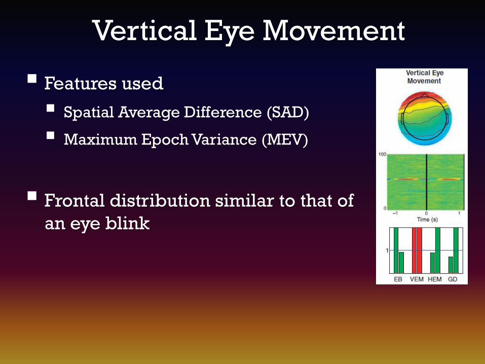
Vertical Eye Movement

Features used



Frontal distribution similar to that of

an eye blink

SAD and MEV

features are over

threshold

Frontal distribution

It appears that the

artifact is mostly

driven by what is

happening around

trial 200

Horizontal Eye Movement

Features used



Frontal distribution in anti-phase

(one positive and one negative)

SED and MEV

features are over

threshold

Anti-phase,

primarily frontal

distribution

In the IC Activity by

trial, three sections

stand out

Trials 110-114

Trial 75-79

Generic Discontinuities

Features used



Variable distribution

Sudden amplitude fluctuations with no spatial preference

Could be present in as little as one or 2 trials, and limited to 1 channel

In component data scroll weird activity in the trial plotted on the IC activity

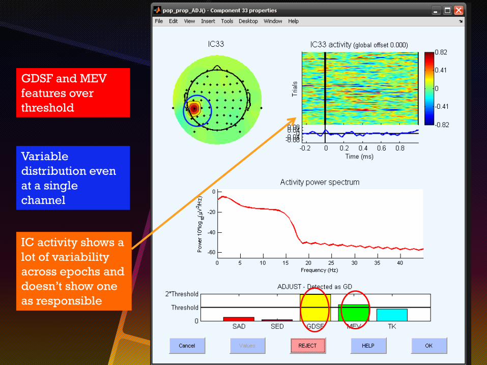
GDSF and MEV

features over

threshold

Variable

distribution even

at a single

channel

IC activity shows a

lot of variability

across epochs and

doesn’t show one

as responsible

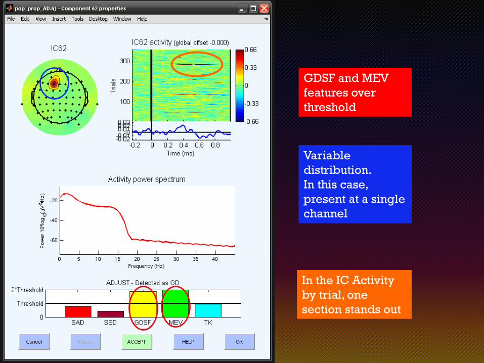
GDSF and MEV

features over

threshold

Variable

distribution.

In this case,

present at a single

channel

In the IC Activity

by trial, one

section stands out

So do we reject all of the ICs

ADJUST tells us too?

If ADJUST has identified a component as bad,

we mark it as bad UNLESS there is clear

evidence that over-rules that verdict.

Additionally, we need to be looking for cases

where ADJUST will miss artifacts

Specially, lateral eye movements seem to be missed

with some frequency in ERP tasks since folks don't

make large movements.

Documents

Processing your EEG Data · 2017-03-08 · Maximum Epoch Variance (MEV) ... Microsoft Word - Processing your EEG Data.docx Author: JJBA Created Date: 4/1/2013 2:20:54 PM