Chapter 11

Processing of Ice Cloud In Situ Data Collected by Bulk Water, Scattering, and ImagingProbes: Fundamentals, Uncertainties, and Efforts toward Consistency

GREG M. MCFARQUHAR,a,b,m DARREL BAUMGARDNER,c AARON BANSEMER,b STEVEN J. ABEL,d

JONATHAN CROSIER,e JEFF FRENCH,f PHIL ROSENBERG,g ALEXEI KOROLEV,h ALFONS

SCHWARZOENBOECK,i DELPHINE LEROY,i JUNSHIK UM,a WEI WU,a,b ANDREW J. HEYMSFIELD,b

CYNTHIA TWOHY,j ANDREW DETWILER,k PAUL FIELD,d,g ANDREA NEUMANN,l RICHARD COTTON,d

DUNCAN AXISA,b AND JIAYIN DONGa

aUniversity of Illinois at Urbana–Champaign, Urbana, IllinoisbNational Center for Atmospheric Research, Boulder, Colorado

cDroplet Measurement Technologies, Boulder, ColoradodMet Office, Exeter, United Kingdom

eUniversity of Manchester, Manchester, United KingdomfUniversity of Wyoming, Laramie, WyominggUniversity of Leeds, Leeds, United Kingdom

hEnvironment and Climate Change Canada, Downsview, Ontario, CanadaiLaboratoire de Météorologie Physique, CNRS/Université Blaise Pascal, Aubière, France

jNorthWest Research Associates, Redmond, Washingtonk South Dakota Schools of Mines and Technology, Rapid City, South Dakota

lUniversity of North Dakota, Grand Forks, North Dakota

ABSTRACT

In situ observations of cloud properties made by airborne probes play a critical role in ice cloud research through

their role in process studies, parameterization development, and evaluation of simulations and remote sensing

retrievals. To determine how cloud properties vary with environmental conditions, in situ data collected during

different field projects processed by different groupsmust be used. However, because of the diverse algorithms and

codes that are used to process measurements, it can be challenging to compare the results. Therefore it is vital to

understand both the limitations of specific probes and uncertainties introduced by processing algorithms. Since

there is currently no universally accepted framework regarding how in situ measurements should be processed,

there is a need for a general reference that describes the most commonly applied algorithms along with their

strengths and weaknesses. Methods used to process data from bulk water probes, single-particle light-scattering

spectrometers and cloud-imaging probes are reviewed herein, with emphasis on measurements of the ice phase.

Particular attention is paid to how uncertainties, caveats, and assumptions in processing algorithms affect derived

products since there is currently no consensus on the optimal way of analyzing data. Recommendations for im-

proving the analysis and interpretation of in situ data include the following: establishment of a common reference

library of individual processing algorithms, better documentation of assumptions used in these algorithms, devel-

opment and maintenance of sustainable community software for processing in situ observations, and more studies

that compare different algorithms with the same benchmark datasets.

1. Introduction

Ice clouds cover ;30% of Earth (Wylie et al. 2005;

Stubenrauch et al. 2006) and make substantial contribu-

tions to radiative heating in the troposphere (Ramaswamy

and Ramanathan 1989). To represent cloud feedbacks in

climate models, the effect of ice clouds on longwave and

mCurrent affiliation: Cooperative Institute for Mesoscale

Meteorological Studies, School of Meteorology, University of

Oklahoma, Norman, Oklahoma.

Corresponding author: Prof. Greg McFarquhar, mcfarq@ou.edu

CHAPTER 11 MCFARQUHAR ET AL . 11.1

DOI: 10.1175/AMSMONOGRAPHS-D-16-0007.1

� 2017 American Meteorological Society. For information regarding reuse of this content and general copyright information, consult the AMS CopyrightPolicy (www.ametsoc.org/PUBSReuseLicenses).

shortwave radiation must be quantified (e.g., Ardanuy

et al. 1991). Ice microphysical processes also affect the

evolution of weather phenomena through impacts on la-

tent heating, which in turn drives the system dynamics. For

example, downdrafts near the melting level in mesoscale

convective systems are forced by cooling associated with

sublimation and melting (e.g., Grim et al. 2009), and the

release of latent cooling at the melting layer feeds back on

the dynamics of winter storms (e.g., Szeto and Stewart

1997). Also, the ice phase is crucial to the hydrological

cycle where most of the time that rain is observed at the

ground it is the result of snow that has melted higher up

(Field and Heymsfield 2015).

To improve the representation of cloud microphysical

processes inmodels, their microphysical properties must

be better characterized because they determine the ice

cloud impact on radiative (e.g., Ackerman et al. 1988;

Macke et al. 1996) and latent heating (e.g., Heymsfield

and Miloshevich 1991). An extensive array of parame-

ters that describes cloudmicrophysical properties can be

derived from microphysical measurements, including

single-particle characteristics (e.g., size, shape, mass or

effective density, and phase), particle distribution

functions [e.g., number distribution functions in terms of

maximum diameterN(Dmax)], and bulk properties (e.g.,

extinctionb, total mass contentwt, medianmass diameter

Dm, effective radius re, and radar reflectivity factor Ze).

Note that all symbols are defined in appendix A.

Past studies have used in situ observations to develop

parameterizations of these microphysical properties. In

particular, parameterizations of N(Dmax) (e.g., Heymsfield

andPlatt 1984;McFarquhar andHeymsfield 1997; Ivanova

et al. 2001; Boudala et al. 2002; Field and Heymsfield

2003; Field et al. 2007; McFarquhar et al. 2007a), wt

(Heymsfield and McFarquhar 2002; Schiller et al. 2008;

Krämer et al. 2016), mass–dimensional relations used

to estimate wt (Locatelli and Hobbs 1974; Brown and

Francis 1995; Heymsfield et al. 2002a,b, 2004, 2010;

Baker and Lawson 2006; Heymsfield 2007; Fontaine

et al. 2014; Leroy et al. 2017), and single-particle light-

scattering properties (Kristjansson et al. 2000; McFarquhar

et al. 2002; Nasiri et al. 2002; Baum et al. 2005a,b, 2007,

2011; Baran 2012; van Diedenhoven et al. 2014) have

been developed. In addition, parameterizations of ef-

fective radius (Fu 1996;McFarquhar 2001;McFarquhar

et al. 2003; Boudala et al. 2006; Liou et al. 2008;

Mitchell et al. 2011a; Schumann et al. 2011) and ter-

minal velocity (Heymsfield et al. 2002b; Heymsfield

2003; Schmitt and Heymsfield 2009; Mitchell et al.

2011b) that rely on measured size and shape distri-

butions have been derived. While such parameteriza-

tions are appropriate for schemes that predict bulk

moments of predefined ice categories (e.g., Dudhia

1989; Rotstayn 1997; Reisner et al. 1998; Gilmore et al.

2004; Ferrier 1994; Walko et al. 1995; Meyers et al. 1997;

Straka and Mansell 2005; Milbrandt and Yau 2005;

Thompson et al. 2004, 2008), there is a new generation of

models (e.g., Sulia and Harrington 2011; Harrington

et al. 2013a,b; Morrison and Milbrandt 2015; Morrison

et al. 2015) that explicitly predict particle properties that

require information about single particles in addition

to bulk properties. In situ data are also needed to

verify and develop retrievals from radar and lidar (e.g.,

Atlas et al. 1995; Donovan and van Lammeren 2001;

Platnick et al. 2001; Hobbs et al. 2001; Frisch et al. 2002;

Mace et al. 2002; Deng andMace 2006; Shupe et al. 2005;

Hogan et al. 2006; Delanoë et al. 2007; Austin et al.

2009; Kulie and Bennartz 2009; Deng et al. 2013).

In situ measurements of ice cloud properties are thus

needed in a variety of cloud types and geographic re-

gimes. Although in situ measurements are commonly

treated as ‘‘ground truth,’’ they are subject to errors and

biases. Thus, uncertainties in derived parameters must

be established to understand the consequences for as-

sociated model and retrieval studies. Knowledge of un-

certainties is also needed for the development and

application of stochastic parameterization schemes

(e.g., McFarquhar et al. 2015). It is difficult to specify a

priori the acceptable uncertainty in a measured or de-

rived quantity that is application dependent. For ex-

ample, studies of secondary ice production (e.g., Field

et al. 2017, chapter 7) might find an error of a factor of 2

in number concentration acceptable, whereas radiative

flux calculations, which require accuracies of 65% for

climate studies (Vogelmann and Ackerman 1995), re-

quire smaller uncertainties. Other chapters in this

monograph better define acceptable levels of un-

certainty for different phenomena.

Measurements from in situ probes are typically

quoted in units of number of particles per unit volume

(e.g., concentration) or mass per unit volume (e.g., mass

content). However, care must be taken when comparing

against output from numerical models where concen-

trations and mass contents are typically represented in

terms of a unit mass of air (e.g., Isaac and Schmidt 2009).

Thus, in situ measured quantities must be divided by the

air density when comparing against modeled quantities.

Caution must also be used when comparing in situ

measurements to remotely sensed retrievals or numer-

ical model output because of differences in averaging

lengths or sample volumes. For example, Fig. 4.11 of

Isaac and Schmidt (2009) demonstrates how average

in situ measured liquid mass contents change with av-

eraging scale, and Wu et al. (2016) demonstrate the

impact of averaging scale on the variability of the sam-

pled size distributions. Finlon et al. (2016) define what

11.2 METEOROLOG ICAL MONOGRAPHS VOLUME 58

represents collocation between in situ and remote

sensing data: they suggest in situ data should be between

250 and 500m horizontally, less than 25m in altitude,

and within 5 s of collocated remotely sensed data. These

discrepancies between in situ and other measurements

should be taken into account when interpreting the re-

sults of processing algorithms presented in this chapter.

Multiple probes are needed to measure microphysical

properties given the wide range of particle shapes, sizes,

and concentrations that exist in nature. Thus, it is critical

to understand the strengths, limitations, uncertainties,

and caveats associated with the derivation of ice prop-

erties from different probes. Two other chapters in this

monograph are dedicated to these issues. Baumgardner

et al. (2017, chapter 9) discusses instrumental problems,

concentrating on measurement principles, limitations,

and uncertainties. Korolev et al. (2017, chapter 5) ex-

amines issues related to mixed-phase clouds, concen-

trating on additional complications in measurements

and related processing that arise when liquid and ice

phases coexist. This current chapter concentrates on an

additional source of uncertainty that has not received as

much attention, namely, that introduced by algorithms

used to process data. Such algorithms play a critical role

in determining data quality. This chapter documents the

fundamental principles of algorithms used to process

data from three classes of probes that are frequently

used to measure cloud microphysical properties: bulk

water, forward-scattering, and cloud-imaging probes.

Although the discussion is slanted toward issues asso-

ciated with derivation of ice cloud properties, it is noted

that these algorithms apply to both liquid water and ice

clouds, as well as to other types of particles, such as

mineral dust aerosols that can be detected by some of

these sensors.

As sensors have developed and evolved, so have the

methodologies for processing, evaluating, and interpreting

the data. Although several prior studies have compared

measurements from different probes or versions of

probes (e.g., Gayet et al. 1993; Larsen et al. 1998; Davis

et al. 2007), fewer studies have systematically compared

or assessed the algorithms used to process probe data

or determined the optimum processing methods and

the corresponding uncertainties in derived products.

For example, most of the previous workshops listed in

Table 11-1 have been dedicated to problems associated

with the measurement of cloud properties, but until re-

cently only the 1984 Workshop on Processing 2D data

(HeymsfieldandBaumgardner1985) concentratedon tech-

niques used to analyze or process measurements. With

this in mind, workshops on Data Analysis and Presenta-

tion of Cloud Microphysical Measurements at the Mas-

sachusetts Institute of Technology (MIT) in 2014 and on

Data Processing, Analysis and Presentation Software at

the University of Manchester in 2016 were conducted.

Many commonly used processing and analysis methodol-

ogies were compared by processing several observation-

ally and synthetically generated datasets, representative

of a range of cloud conditions. This article reviews and

extends the proceedings and findings of these workshops.

In particular, the basis and uncertainties in algorithms for

bulk water, forward-scattering, and cloud-imaging probes

are described, different algorithms designed to process

data are compared, and future steps to improve process-

ing of cloud microphysical data are suggested.

2. Probes measuring bulk water mass content

Chapter 9 (Baumgardner et al. 2017) describes the

operating principle of heated sensor elements, their basis

for detection and derivation of water mass content,

measurement limitations, and uncertainties. In this sec-

tion, the fundamental method of processing data from

heated sensors based on thermodynamic principles is

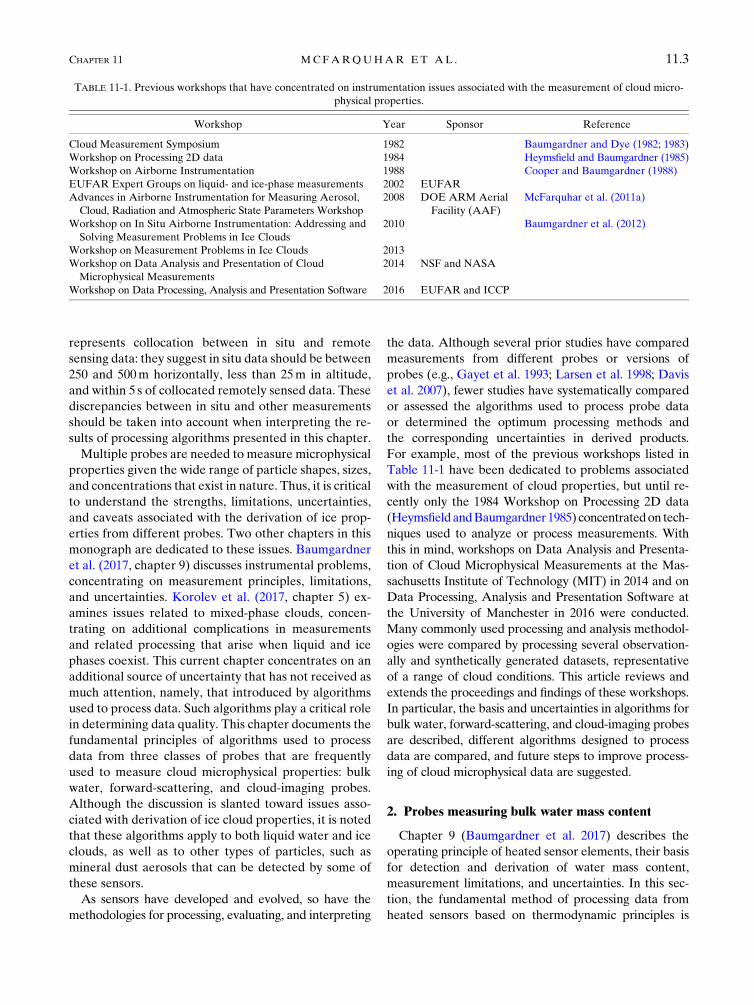
TABLE 11-1. Previous workshops that have concentrated on instrumentation issues associated with the measurement of cloud micro-

physical properties.

Workshop Year Sponsor Reference

Cloud Measurement Symposium 1982 Baumgardner and Dye (1982; 1983)

Workshop on Processing 2D data 1984 Heymsfield and Baumgardner (1985)

Workshop on Airborne Instrumentation 1988 Cooper and Baumgardner (1988)

EUFAR Expert Groups on liquid- and ice-phase measurements 2002 EUFAR

Advances in Airborne Instrumentation for Measuring Aerosol,

Cloud, Radiation and Atmospheric State Parameters Workshop

2008 DOE ARM Aerial

Facility (AAF)

McFarquhar et al. (2011a)

Workshop on In Situ Airborne Instrumentation: Addressing and

Solving Measurement Problems in Ice Clouds

2010 Baumgardner et al. (2012)

Workshop on Measurement Problems in Ice Clouds 2013

Workshop on Data Analysis and Presentation of Cloud

Microphysical Measurements

2014 NSF and NASA

Workshop on Data Processing, Analysis and Presentation Software 2016 EUFAR and ICCP

CHAPTER 11 MCFARQUHAR ET AL . 11.3

reviewed, focusing on the Nevzorov and King probes. In

addition, algorithms deriving wt from evaporator probes,

namely, the Counterflow Virtual Impactor (CVI; note

that all acronyms are defined in appendix B) and Cloud

Spectrometer and Impactor Probe (CSI), are reviewed.

Processing algorithms for other bulk total water probes—

such as the Scientific Engineering Applications (SEA)

hot-wire Robust probe (Lilie et al. 2004); the SEA Iso-

kinetic Evaporator Probe (IKP2), specifically designed

formeasuring highwt at high speeds (Davison et al. 2009);

and the Particle Volume Monitor (PVM; Gerber et al.

1994)—are not discussed because there are not multiple

algorithms for processing these data, and when there are,

there is minimal variation between algorithms.

Although the King probe was designed to measure

liquid water content wl, its sensor does respond to ice

(e.g., Cober et al. 2001) but in an unpredictable manner.

Processing algorithms for theKing andNevzorov probes

have many common features, and both are discussed in

this chapter.While theKing probe has a single sensor for

sampling liquid, the Nevzorov probe has two sensors:

one for measuring wl and another for measuring wt. The

determination ofwl from the King and Nevzorov probes

is discussed here because the processing concepts assist

in understanding how wt is derived and because wl is

needed for a characterization of mixed-phase clouds.

The King and Nevzorov probes are referred to as ‘‘first

principle’’ instruments because the heat lost from the

sensor through the transfer of energy via radiation, con-

duction, convection, and evaporation of droplets can be

directly calculated based on thermodynamic principles.

The first two components are usually ignored because

their contribution to the total power is negligible com-

pared to the other two terms. Thus, the powerW required

to keep the wire at a constant temperature Tw is given by

W5 ldVwl[L

y1 c(T

w2T

a)]1P

D, (11-1)

where the first term (wet term) is the heat required to

warm the droplets from the ambient temperature Ta to

Tw and evaporate them, and the second term (PD dry

term) is the heat transferred to the cooler air moving

past the wire. In Eq. (11-1), l and d are the length and

diameter of the cylinder, V is the velocity of air passing

over the sensor,Ly is the latent heat of vaporization, and

c is the specific heat of liquid water. To extract wl, the

energy lost to the air PD must be subtracted from the

total energy consumed. This procedure is implemented

differently in the King and Nevzorov probes.

a. Dry term estimation for King probe analysis

The King probe (King et al. 1978) consists of a thin

copper wire wound on a hollow 1.5-mm-diameter

cylinder. It estimates wl through the electrical current

required to maintain the sensor at a constant tempera-

ture (Baumgardner et al. 2017, chapter 9). This is an

improvement over its predecessor, the Johnson–William

probe, which heated a 0.5-mm-diameter wire with an

electrical current as part of a bridge circuit at a constant

current but not constant temperature.

King et al. (1978) suggested that the dry term PD

could be parameterized by PD 5 b0(Tw 2 Ta)Rex,

where Re is the Reynold’s number and the x and

b0 parameters are established in either a wind tunnel or

from flight measurements. Recent investigations at

NCAR and the University of Wyoming (A. Rodi 2016,

personal communication). have established that the

Zukauskas and Ziugzda (1985) method gives a better

representation of PD in terms of Re and the Prandtl

number evaluated at the film and wire temperatures

Tf and Tw, respectively.

The Tf, Tw, Ta, V, and the air pressure P must be

known to determine the dry term PD. The temperature

in a region near the sensor is Tf and is assumed to be the

average of Tw and Ta. This however, remains an un-

tested assumption. In addition, there are major un-

certainties in determiningTw andV sinceV is usually not

identical to the velocity of the aircraft because of airflow

distortions in the sensor’s vicinity (Baumgardner et al.

2017, chapter 9).

There are two approaches to estimating the dry-air

term. The constant altitude method (CAM) is prefera-

bly implemented on a cloud-by-cloud basis. The power

is measured prior to and after cloud penetration and

averaged to obtain the dry-air term for one cloud pass.

This approach makes the following assumptions: 1) the

presence of cloud can be detected with another in-

strument or through some thresholding technique to use

the hot-wire sensor as a cloud detector, and 2) Ta, P, and

V do not vary significantly (typically ,10%) inside or

outside the cloud.

The optimum parameterization method (OPM) re-

quires an estimate of Tf and a factor Vf, to correct the

aircraft velocity to the velocity over the sensor. The

velocity correction factor is assumed constant for a

particular mounting location. This approach also as-

sumes that there is a way to detect clouds so that only

cloud-free measurements are used in the calculation.

The parameter estimates can be made over a whole

project, over one flight, or as a function of altitude. The

following steps obtain the optimum values: 1) select a

value for Tf and Vf; 2) compute PD for every measured

data point; 3) calculate an error metric between the

measured power Pm and PD, for example, S(Pm 2 PD)2;

4) check if the error is above a threshold value; and if it

is, 5) adjust Tf, and Vf and return to step 1.

11.4 METEOROLOG ICAL MONOGRAPHS VOLUME 58

For the MIT workshop, the OPM and CAM methods

were applied to an unprocessed raw dataset supplied by

the NCAR Research Applications Laboratory (RAL).

The measurements were made with a Particle Measur-

ing Systems (PMS) LWC hot-wire sensor mounted on

the Aerocommander aircraft flown during the 2011

Cloud–Aerosol Interaction and Precipitation Enhance-

ment Experiment (CAIPEEX) over the Indian Ocean.

The clouds sampled were all liquid water with no ice.

Figure 11-1 showswl derived from the raw data using the

CAM and OPM methods and their average, compared

with the results from processing performed at RAL

using a constant wire temperature and dry-air term pa-

rameterized by the Reynolds and Prandtl numbers

(Zukauskas and Ziugzda 1985). The differences be-

tween the two techniques are negligible.

b. Nevzorov probe analyses

As discussed in Baumgardner et al. (2017, chapter 9), the

Nevzorov hot-wire probe (Korolev et al. 1998a, 2013a)

consists of a heated cone mounted on a moveable vane to

measure wt and a heated wire wound onto a copper rod to

measure wl, with wt 5 wl 1 wi. Liquid droplets impacting

either sensor should evaporate fully, but ice particles tend to

break up and fall away from the liquid water sensor,

although a residual signal from these ice particles is often

observed (Korolev et al. 1998a). As the heated sensors are

exposed to the airflow, forced convective cooling adds to the

power requirement to melt and evaporate cloud particles.

The cooling depends on the aircraft attitude and environ-

mental conditions. A reference sensor partially compen-

sates for this convective cooling and enables removal of

most of the dry-air heat-loss term. Assumingwl5 0, the ice

water content (wi) in ice clouds can be calculated following

wi5

PC2KP

R

VSL*, (11-2)

where PC and PR are the collector and reference sensor

power, S is the sensor sample area, L* is the energy re-

quired to melt and evaporate measured hydrometeors,

andK is the ratio of the collector to reference power that

is dissipated in cloud-free air representing the dry-air

heat loss term. The lack of full compensation for this

term by the reference sensor leads to a variation in K

during a flight and hence a ‘‘baseline drift’’ of the cal-

culated wi. Korolev et al. (1998a) and Abel et al. (2014)

show that K is dependent on V and environmental

conditions. The probe precision in wi can reach

60.002 gm23, providing that the baseline drift is re-

moved by adequately capturing how K varies over the

flight (Abel et al. 2014). In the event wl 6¼ 0, more

complications arise because the liquid sensor partially

responds to ice, so even subtracting wl from wt gives a

larger error in the estimated wi.

Nevzorov data from three flights were processed for

the 2014 workshop by two groups that were not pub-

licly identified, henceforth represented as G1 and G2.

The data were from two flights of the University of

North Dakota Citation II aircraft, one within a trailing

stratiform region of a mesoscale convective system

and the other from a flight in supercooled convective

showers. The third dataset was from a flight in mid-

latitude cirrus on the FAAM BAe-146 research air-

craft. Both groups characterized the baseline drift of

the probe by looking at how K varied as a function of

indicated airspeed (IAS) and P. The groups, however,

used different functional forms. G1 calculated DK 5a1D(1/IAS)1 a2Dlog10(P) and G2 calculatedK asK5b1IAS1 b2P1 b3. The coefficients a1, a2, b1, b2, and b3were calculated on a flight-by-flight basis using cloud-

free data points.

Figure 11-2 shows PC/PR,K (i.e., the baseline), and wt

derived by G1 and G2 denoted wtG1 and wtG2, re-

spectively. The different parameterizations ofK capture

similar trends in the baseline drift for each flight, with

small offsets on two of the flights. The impact of these

offsets leads to systematic biases in the calculation of wt,

with the largest mean difference wtG1 2 wtG2 being as

high as20.011 gm23 for the convective cloud flight. An

indication of the agreement between data processed by

the two groups is given by the61s values ofwtG12wtG2,

FIG. 11-1. Mass content wl derived by DMT, using CAM and

OPM as a function of wl derived using a constant wire temperature

and dry-air term parameterization by the Reynolds and Prandtl

numbers (Zukauskas and Ziugzda 1985) for measurements made

with a PMS LWC hot-wire sensor mounted on the Aero-

commander aircraft during the 2011 CAIPEEX over the Indian

Ocean. The clouds sampled were all liquid water with no ice.

CHAPTER 11 MCFARQUHAR ET AL . 11.5

which are60.002,60.002, and60.003gm23 for the three

flights.

c. CVI and CSI analysis

The CVI/CSI condensed water measurement is based

on water vapor measured directly after hydrometeor

evaporation or sublimation in the inlet of the instrument

(Noone et al. 1988; Twohy et al. 1997). As described in

chapter 9 (Baumgardner et al. 2017), the water vapor

from evaporated cloud droplets or ice crystals is mea-

sured downstream, typically by a tunable diode laser

(TDL) hygrometer. Most accurate results are obtained

when the hygrometer is calibrated for the full range of

pressures and water vapor contents that will be en-

countered, generating a nonlinear coefficient matrix

that is a function of both vapor concentration and

pressure. The basic processing involves applying the

calibration to the measured vapor content and dividing

by an enhancement factor. The enhancement factor is

calculated as the volumetric flow of air ingested by the

CVI/CSI probe tip (airspeed multiplied by cross-

sectional area) divided by the total volumetric flow of

air inside the CVI inlet (sum of all downstream flow

rates that are continuously monitored). The root-sum-

square uncertainty using a TDL sensor is estimated

as 611% for 0.05 , wt , 1.0 gm3, 615% at 0.05 gm3,

and 623% for wt # 0.025 gm3 (Heymsfield et al. 2006;

Davis et al. 2007).

Special processing can be applied for additional ac-

curacy. Outside cloud, the measured wt should be zero,

since ambient air is prevented from entering the inlet

by a counterflow, and dry gas is recirculated throughout

the internal system. Depending on the response of the

water vapor sensor to changing pressure, a small base-

line offset may remain after calibration. This precloud-

entry baseline offset may be removed from in-cloud data

before the enhancement factor is applied. At high wt,

water vapor inside the inlet may saturate or exceed the

capabilities of the sensor, leading to saturation flatlin-

ing of the signal. This problem can be minimized by

FIG. 11-2. (left) Measured PC/PR (black) from Nevzorov wt sensor. Cases include data from (top) a trailing

stratiform region of amesoscale convective system collected using theUniversity of NorthDakota (UND)Citation,

(middle) supercooled convective showers collected using the UND Citation, and (bottom) midlatitude cirrus

collected using the FAAM BAe-146 research aircraft. K parameter calculated by G1 and G2 shown in red and

green, respectively. (right) Comparison of the calculated wt from G1 and G2. The red line is the 1:1 line.

11.6 METEOROLOG ICAL MONOGRAPHS VOLUME 58

adjusting flow rates during flight to decrease the en-

hancement factor. Hysteresis may also occur through

incomplete evaporation or water vapor adhering to in-

ternal surfaces, which results in water vapor being

measured subsequent to cloud sampling. For sharper

time resolution, the water vapor in the postcloud hys-

teresis tail can be added back to the in-cloud signal,

using cloud exit time determined from other cloud

sensors.

3. Light-scattering spectrometers

Chapter 9 (Baumgardner et al. 2017) describes the

operating principle of light-scattering probes. These

spectrometers were originally developed to measure the

size distributions of liquid water and supercooled water

droplets, but with appropriate modifications in pro-

cessing algorithms can also provide information about

N(Dmax) in ice clouds. From the measured N(Dmax),

other properties such as total number concentration,

effective radius and water content can be derived. In this

section, the fundamental methods of processing data

from light-scattering spectrometers are discussed, and

comparisons between different algorithms are made.

The discussion centers around algorithms used to

process data from probes that scatter light in the forward

direction. These instruments include the Forward Scat-

tering Spectrometer Probe (FSSP), a legacy probe

originally manufactured by PMS and Particle Metrics

Incorporated (PMI); the revised signal-processing

package (SPP-100), an FSSP with electronics upgraded

to eliminate dead time and manufactured by DMT; the

Cloud Droplet Probe (CDP), Cloud and Aerosol Spec-

trometer (CAS), and CDP-2 with upgraded electronics,

all manufactured by DMT; the Fast FSSP (FFSSP), an

FSSP retrofit with upgraded (fast) electronics and probe

tips, and the Fast Cloud Droplet Probe (FCDP), which

is a unique design with fast electronics, both of which are

manufactured by SPEC. Probes that measure scattering

in multiple directions [e.g., the small ice particle de-

tector (SID) or polar nephelometers], in the backward

direction [e.g., Backscatter Cloud Probe (BCP)] or in-

cluding polarization [e.g., Cloud and Aerosol Spec-

trometer with Polarization (CAS-POL), Backscatter

Cloud Probe with Polarization Detection (BCPD), or

the Cloud Particle Spectrometer with Polarization De-

tection (CPSPD)] are not discussed because there is

more variation in algorithms used to process data from

these spectrometers. Although the basics of algorithms

are identical for liquid water and ice particles, there are

additional uncertainties in sizing nonspherical ice par-

ticles described at the end of this section. Beyond the

sizing of nonspherical particles and the inescapable

sampling uncertainty (Hallett 2003), there are two other

major sources of error in calculating the number con-

centration: coincidence and shattering.

a. Adjustments for coincidence

Coincidence occurs when more than one particle is

within the sensor’s laser beam. The impact of this event

depends on the relative position of the particles. Parti-

cles coincident in the qualified sample area (SAQ) are

counted as a single, oversized particle. But, when one

particle is in the SAQ and the other outside SAQ, but in

the extended sample area [SAE; i.e., particles detected

by the sizer that transit outside the SAQ; see chapter 9

(Baumgardner et al. 2017) and Fig. 2 in Lance (2012) for

the definitions of SAQ and SAE and more details on the

operation of forward-scattering probes], the particles

will be missized and possibly even rejected depending

on their relative sizes (Baumgardner et al. 1985;

Brenguier andAmodei 1989; Brenguier 1989; Brenguier

et al. 1994; Cooper 1988; Lance 2012). Lance (2012)

describes an optical modification to a CDP that places

an 800-mm-diameter pinhole in front of the sizing de-

tector. This reduces particle coincidence in the SAE

because otherwise unqualified drops that transit outside

the SAQ can still be detected by the sizer. Nevertheless,

even with a SAE of 2.7mm2 in the modified CDP (Lance

2012) and a beamwidth of 200mm, a sample volume of

0.54mm3 means more than one particle will be detected

in the SAE for concentrations greater than 1850 cm23,

assuming a uniform spatial distribution of particles.

However, as particles are randomly distributed or per-

haps clustered (e.g., Paluch and Baumgardner 1989;

Baker 1992; Pinsky and Khain 1997; Davis et al. 1999;

Kostinski and Jameson 1997, 2000), the data still need to

be adjusted to account for the effect of coincidence.

Previously these adjustments have been called cor-

rections; however, the term ‘‘corrections’’ suggests that

there is a priori knowledge of the actual size distribution,

which is typically not the case. Thus, the term ‘‘adjust-

ments’’ is used henceforth. Note that it is especially

important to adjust for coincidence when very high

particle concentrations are present or at lower concen-

trations when processing data from unmodified probes

(e.g., an SAE of 20.5mm2 for the unmodified CDP sug-

gests more than one particle in the sample volume for

concentrations greater than 243 cm23).

Coincidence events cannot be avoided, but statistical

or empirical adjustments, as well as alternatemethods of

particle counting, are possible. Statistical adjustments

assume that particles are randomly distributed in space

and that the probability of a particle in the beam is given

by 1 2 e2lt where t is the average transit time of a

particle in the depth of field (DOF) and l is the particle

CHAPTER 11 MCFARQUHAR ET AL . 11.7

detection rate, where l 5 NaADOFV (Baumgardner

et al. 1985) with Na the ambient particle number con-

centration,ADOF theDOF area andV the velocity of the

air passing over the sensor. The relationship between

the measured number concentration Nm and Na is ap-

proximated by Baumgardner et al. (1985) as

Nm5N

a(T2 t

d)e2lt/T , (11-3)

where T is the sampling period and td is the cumulative

dead time during the time of the sample interval. The

dead time corresponds to the time required to reset the

electronics after a particle has left the beam. During this

reset period the probe does not detect particles. This

nonlinear relationship can be solved iteratively for Na.

Another adjustment method requires either a direct

measurement or estimate of the probe activity a. Ac-

tivity is the fraction of the sampling interval that the

instrument is processing a particle, including the time a

particle has been detected in the beam, either within or

outside the DOF, and the dead time. The dead time is

only relevant for the legacy FSSPs manufactured by

PMS and PMI, and SID-type instruments that have a

fixed dead time after each particle. Legacy FSSPs that

have been modified with the DMT SPP-100 electronics

do not suffer from dead time. The adjustment factorCf is

given by

Cf5 (12ma)21 , (11-4)

where m is a probe-dependent adjustment factor and

Na5C

fN

m. (11-5)

Original manufacturer recommendations suggest a

value of m between 0.7 and 0.8. However, simulations

have shown that this may vary from 0.6 to 0.8

(Baumgardner et al. 1985), and values as low as 0.54

(Cerni 1983) can be found in the literature. Brenguier

(1989) suggests the value lies between 0.5 and 0.8. More

studies are needed to establish a value form that may be

probe dependent. For the CDP and CAS, the activity

can be approximated by

a5 nmT

s/T , (11-6)

where nm is the number of particles counted in sample

interval T, and Ts is the average transit time; however, a

value for m has yet to be derived for these probes.

A similar approach uses the measured activity but

takes into account probe-specific parameters such as

laboratory-measured electronic delay times including

dead time and time response of amplifiers, beam di-

ameter, and DOF (Dye and Baumgardner 1984). This

statistical approach models the behavior of the probe

assuming droplets passing through the sample volume

are uniformly distributed in space with a constant mean

density (Brenguier and Amodei 1989). The algorithm

computes an actual concentration by estimating the

probability of a coincidence event based on the activity

and other probe parameters. An equivalent m can be

determined using Eqs. (11-4) and (11-5), but the equiv-

alent m will vary such that it asymptotically approaches

1 with increasing droplet concentration. The value of m

depends on probe-specific parameters and on the transit

time of individual particles (Brenguier 1989). No simple

functional relationship exists between m and a. For the

data presented by Brenguier (1989), the minimum m

was less than 0.6 at low activities but exceeded 0.8 for

higher activities.

Examples of the above two methodologies are com-

pared for data collected by an FSSP on the University

of Wyoming King Air in convective clouds with drop-

let concentrations in excess of 1000 cm23 during the

Convective Precipitation Experiment (COPE) in 2013

over southwest England. Data from 3 separate days

were selected for analysis from penetrations where

no significant precipitation-sized particles were de-

tected by the imaging probes. Figure 11-3a shows three

coincidence-adjusted estimates of droplet concentration

as a function of Nm. The red and blue circles show the

coincidence-adjusted concentrations using a constant m

of 0.54 and 0.71, respectively, and green circles show the

concentrations adjusted using the method of Brenguier

and Amodei (1989). The solid line indicates the 1:1 line

and dashed lines show 20%, 50%, and 100% adjust-

ments to Nm. For Nm , 200 cm23, coincidence adjust-

ments are less than 20%. For 200 , Nm , 400 cm23,

coincidence adjustments may be as large as 75% with

differences depending on the chosen value form. In this

range of Nm, differences between adjusted concentra-

tions are small when comparing the Brenguier and

Amodei (1989) method with the method of a fixed m

equal to 0.71. For Nm . 500 cm23, coincidence adjust-

ments may exceed 100% and differences between

using a fixed m of 0.71 and the statistical model of

Brenguier and Amodei (1989) approach 20%.

The same three coincidence-adjusted FSSP concen-

trations are shown in Fig. 11-3b and plotted as a function

ofNm from aCDP. TheCDPhad beenmodifiedwith the

‘‘pinhole’’ to reduce impacts of coincidence (Lance et al.

2010; Lance 2012) and the sample volume was measured

by the probe manufacturer. Coincidence-adjusted con-

centrations from the FSSP agree to within 20% of

measured CDP concentrations for Nm , ;500 cm23.

For larger Nm, coincidence-adjusted concentrations for

the FSSP using a fixedm of 0.71 or the statistical method

11.8 METEOROLOG ICAL MONOGRAPHS VOLUME 58

of Brenguier and Amodei (1989) also agree to within

20% of the CDP measurements, but the lower value of

fixed m (0.54) predicts significantly lower concentration

compared to those measured by the CDP.

Instruments that measure the individual particle-by-

particle (PbP) interarrival times (i.e., the FCDP, FFSSP,

CDP-2, and CPSPD) allow a precise estimate of activity

but do not avoid coincidence. For these probes, a con-

centration that is almost unaffected by coincidence can

be derived. The standard method for calculating con-

centration is Nm 5 nm/SV, where SV is the sample vol-

ume given by SAVT. An alternative definition is Nm 5nm/SAVSt, where St is the sum of interarrival times,

and SA is the appropriate sample area.

A final approach uses an inversion technique

(Twomey 1977; Markowski 1987) to derive ambient size

distributions (SDs) from those measured. Here the in-

strument’s operating principles are modeled, and its

response to ambient particles predicted and compared

to actual measurements. Estimates of the ambient SD

are adjusted until the predicted response matches that

measured within a preset error. This approach has been

implemented with the BCP (Beswick et al. 2014, 2015)

and should be equally effective with other scattering

probes when the operating characteristics have been

evaluated. As physical models of scattering probes be-

come even more robust, the utility of inversion tech-

niques toward nudging measurements toward realistic

values will become even greater.

b. Sizing

The simplest case of using a light-scattering spec-

trometer for sizing is for spherical water droplets. The

amount of scattered light can be derived directly from

Mie–Lorenz theory. Deriving sizes for ice crystals is

more complex because every crystal is unique and has

the potential for different alignments with respect to

the laser.

However, even for the droplet case, effectively de-

riving particle sizes is nontrivial. Two fundamental

problems exist. First, as predicted by Mie–Lorenz the-

ory, the amount of light scattered by a particle is not a

monotonic function of diameter. The peaks and troughs

in the relationship are often referred to as Mie–Lorenz

oscillations and their amplitude is particularly significant for

droplets smaller than ;15mm [chapter 9 (Baumgardner

et al. 2017) discusses the sources of this uncertainty].

The second problem is that the properties of the instru-

ments are often not well constrained. These properties

include uncertain scattering angular sizes and imperfect

alignment of apertures and beam blockers, variation in

illumination intensity over the sample volume, uncertain

instrument sensitivity and offset, and the amount of

electronic noise. These items cause smoothing of the

Mie–Lorenz oscillations or broadening of the distribution

(i.e., a particle-to-particle variability even for identical

diameters). Because the amount of light scattered is

highly nonlinear, the impacts of broadening do not cancel

in themean as theymight in a linear system. For example,

if a peak in the Mie–Lorenz curve occurs just below a

threshold between two sizing bins, then broadening

would cause a large fraction of particles at this size to

jump up into the next bin. If no trough exists just above

this threshold very few particles would jump down from

this higher bin, and hence the impact of broadening

would be to generate a bias.

FIG. 11-3. (left) Activity-based coincidence-corrected concentration as a function of raw (measured) concen-

tration from the FSSP for values of fixedm of 0.54 (red) and 0.71 (blue) and for the statistical method of Brenguier

and Amodei (green) for data collected during 2013 COPE over southwest England using the University of

Wyoming King Air for 3–4-min penetrations on 3 days during periods that did not appear to contain any pre-

cipitation-sized particles. (right) Activity-based coincidence-corrected concentrations from the FSSP for the same

dataset shown in (left), but compared to measured concentrations from a CDP on the same aircraft.

CHAPTER 11 MCFARQUHAR ET AL . 11.9

The best efforts of the community to date to perform

sizing using light-scattering spectrometers involve cali-

brating using well-characterized particles. The calibra-

tion particles are usually spherical glass beads (e.g.,

Gayet 1976; Pinnick and Auvermann 1979; Cerni 1983;

Dye and Baumgardner 1984), polystyrene latex nano-

spheres (Nagel et al. 2007), liquid water droplets from a

controlled jet (Wendisch et al. 1996; Nagel et al. 2007),

or in some cases ice crystal analogs. An adjustment must

be made if the calibration particles are not the same

material as the particles being measured; this is called a

refractive index adjustment, typically referred to as a

refractive index correction in the literature. The process

is nontrivial because of theMie–Lorenz oscillations. The

scattered light measured by the instrument s is expected

to be a nonmonotonic function of particle size.

Some studies (see Baumgardner et al. 2017, chapter 9)

have indicated that the predicted oscillations of as much

as 300% between 3 and 10mm and of up to 50% at di-

ameters greater than 10mm in forward-scattering probes

are not well observed though the unavailability of many

closely sized and narrowly distributed calibration sam-

ples limits mapping of the oscillations. However, if an

instrument is calibrated using material similar to the

measured particles, it may be sensible to utilize an em-

pirical monotonic response curve that approximates the

calibration points (e.g., Cotton et al. 2010; Lance

et al. 2010).

The problem with using an empirical monotonic re-

sponse curve is that if an instrument is responding to

Mie–Lorenz oscillations, then artifacts will be created,

such as false peaks and troughs. Further, it is not obvious

how to perform refractive index corrections when the

calibration samples are a different composition than the

in situ samples. To attempt to counter these issues,

Rosenberg et al. (2012) recommends the calibration of

bin boundaries in terms of the scattered light measured

by the forward-scattering instrument s (which is a linear

function of instrument response) rather than the sizeD;

then integration over ranges of D that fall in each s bin

give each bin amean diameter and effective width rather

than two bin edges. The advantages of this approach are

that s can be a nonmonotonic function of D (which

could, for example be based onMie–Lorenz theory) and

uncertainties from the calibration can be rigorously

propagated including ambiguities from nonmonotonic

s(D). However, this method is simply a numerical

technique for refractive index correction based on a

user-supplied function s(D). If this user-supplied func-

tion is incorrect, because the sizes and alignments of the

instrument aperture and beam blocker are unknown, the

method will generate artifacts. The method can be re-

peated with multiple versions of s(D) to determine the

uncertainty in sizing due to the uncertainty in this

function. This method does incorporate the impacts of

broadening mechanisms described above; however, the

way this method integrates over the range of calibration

uncertainties may have a similar impact to the broad-

ening mechanisms.

Figure 11-4 shows an example of a size distribution

from a CDP in a fair-weather cumulus (taken from

FAAM flight B792) and a 3–30-mm polydisperse bead

sample (provided by Whitehouse Scientific) plotted us-

ing the manufacturer’s specifications and using the

Rosenberg et al. (2012) method. The bead sample has

had its cumulative volume distribution calibrated in the

range ;9–12mm. A cumulative lognormal curve has

been fit to the provided calibration points, and then

subsequently converted to a number distribution. Two

versions of the Rosenberg et al. (2012) method have

been applied. One using s calculated using the standard

CDP light collection angular range of 48–128, and one

using the range 1.78–148 recommended by the manu-

facturer for this instrument. The difference between the

two angular ranges gives an indication of how sensitive

the method is to the chosen s(D) and how uncertainties

in this function may propagate. No attempt is made to

include the effect of optical misalignments because

there is no indication of how large such misalignments

may be. These data are presented to highlight how a size

distribution can vary greatly through different process-

ing methodologies based on seemingly sensible as-

sumptions. With no calibration applied, there are three

peaks in the cloud distribution below 20mm and three

peaks at the same diameters in the polydisperse bead

distribution. The fact that these three peaks occur in the

unimodal bead distribution indicates that they are likely

artifacts.

With the Rosenberg method applied and based on the

size of the error bars presented by this method, it would

be concluded that this is a bimodal distribution and a

bimodal best fit curve is shown. However, the Rosen-

berg method also produces two modes for the unimodal

bead distribution: one at approximately the correct size

and one at a larger size. This of course casts doubt on its

use for in situ measurements. The additional peak could

be caused by an incorrect s(D) (wrong scattering an-

gular range or failure to account for misalignment);

failure to account for broadening effects; or a problem

with the delivery of the sample, for example, co-

incidence (as described in section 3c) causing particle

oversizing generating an actualmode of larger aggregate

particles. This example shows how difficult it is to

create a methodology and validate its ability to effec-

tively size particles within a rigorously defined un-

certainty. This is due to limitations first in models of the

11.10 METEOROLOG ICAL MONOGRAPHS VOLUME 58

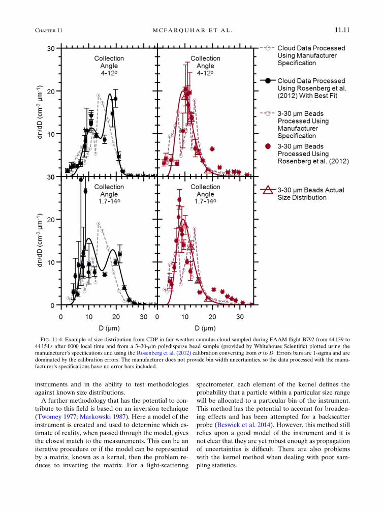
instruments and in the ability to test methodologies

against known size distributions.

A further methodology that has the potential to con-

tribute to this field is based on an inversion technique

(Twomey 1977; Markowski 1987). Here a model of the

instrument is created and used to determine which es-

timate of reality, when passed through the model, gives

the closest match to the measurements. This can be an

iterative procedure or if the model can be represented

by a matrix, known as a kernel, then the problem re-

duces to inverting the matrix. For a light-scattering

spectrometer, each element of the kernel defines the

probability that a particle within a particular size range

will be allocated to a particular bin of the instrument.

This method has the potential to account for broaden-

ing effects and has been attempted for a backscatter

probe (Beswick et al. 2014). However, this method still

relies upon a good model of the instrument and it is

not clear that they are yet robust enough as propagation

of uncertainties is difficult. There are also problems

with the kernel method when dealing with poor sam-

pling statistics.

FIG. 11-4. Example of size distribution from CDP in fair-weather cumulus cloud sampled during FAAM flight B792 from 44 139 to

44 154 s after 0000 local time and from a 3–30-mm polydisperse bead sample (provided by Whitehouse Scientific) plotted using the

manufacturer’s specifications and using the Rosenberg et al. (2012) calibration converting from s to D. Errors bars are 1-sigma and are

dominated by the calibration errors. The manufacturer does not provide bin width uncertainties, so the data processed with the manu-

facturer’s specifications have no error bars included.

CHAPTER 11 MCFARQUHAR ET AL . 11.11

All of the previous discussion has been concerned

with spherical particles that have well-understood light-

scattering properties. There are few studies that have

developed techniques to adjust SDs for the impact of

coincidence, incorrect DOF, or missizing of ice crystals.

Cooper (1988) illustrated an inversion technique that

models the response of the FSSP to particles coincident

in the beam, showing that an ambient SD can be derived

from the measured SD. But, this issue needs more study

to improve its accuracy, especially when concentrations

are elevated. Borrmann et al. (2000) and Meyer (2013)

employed T-matrix calculations to estimate the sizing of

oblate spheroids of varying aspect ratios in order to in-

vestigate the derivation of a response function from ice

crystals. The surface roughness and occlusions in ice

crystals also impact their scattering properties. No sys-

tematic adjustments are currently being applied to

measurements in mixed- or ice-phase clouds to account

for nonspherical shapes or surface roughness partly be-

cause of uncertainties in how to represent small crystal

shape (e.g., Um and McFarquhar 2011) and roughness

(e.g., Collier et al. 2016; Magee et al. 2014; Zhang

et al. 2016).

c. Shattering adjustments

It has been conclusively established that shattering

of large ice crystals on the tips or protruding inlets can

artificially amplify the concentrations measured by

forward-scattering probes (Gardiner and Hallett 1985;

Gayet et al. 1996; Field et al. 2003; Heymsfield 2007;

McFarquhar et al. 2007b, 2011b; Jensen et al. 2009; Zhao

et al. 2011; Febvre et al. 2012; Korolev et al. 2011, 2013b,

c). In addition to the use of redesigned probe tips, the

elimination of particles with short interarrival times can

mitigate the presence of many artifacts. But, as discussed

in section 4 as pertains to optical array probes (OAPs),

the implementation of such algorithms can add un-

certainties to ice crystal concentrations. Such algorithms

can only be applied to the spectrometer probes that re-

cord individual particle-by-particle interarrival times.

4. Imaging probe analysis

a. Introduction and generation of synthetic data

Chapter 9 (Baumgardner et al. 2017) describes the

operating principles of imaging probes and lists the

different types in Table 9-1. Imaging probes include

both OAPs that provide 10-mm or coarser-resolution

images [e.g., Cloud Imaging Probe (CIP), Precipitation

Imaging Probe (PIP), 2DS, HVPS-3 and the 2DC and

2DP legacy probes originally developed by PMS] as well

as probes providing higher-resolution images through

different operating principles (e.g., CPI, HOLODEC,

PHIPS-HALO, HSI). Although analysis characterizing

particle morphology and identifying particle habits

are common to all imaging probes, procedures to derive

N(Dmax) and total concentrations differ for OAPs and

other probes because of the different manner in which

sample volumes are defined. In this section, image

analysis algorithms that can be applied to any class of

probe are discussed. However, algorithms deriving

N(Dmax) are discussed only for OAPs since such algo-

rithms can be applied to a number of different probes

and because many algorithms developed by different

groups are available. The discussion does not focus on

algorithms for specific probes, but rather concentrates

on examining aspects of algorithms that are common to

all OAPs (e.g., those manufactured by PMS, DMT, or

SPEC, Inc.). Algorithms for deriving N(Dmax) from the

higher-resolution imagers are not discussed here as they

tend to be more specialized, applicable only to a single

probe, with typically only a single algorithm developed

by the instrument designer available.

To compare processing algorithms, a synthetic dataset

simulating data generated by OAPs was developed at

NCAR.1 The simulation includes all major aspects of

OAP performance and operation, including an optical

model, an electronic delay and discretization model,

particle timing information, airspeed, array clocking

speed, and raw data compression and encoding. It starts

with the definition of model space and characteristics of

the probe to be simulated, such as the number of diodes,

arm spacing, diode resolution, and diode response

characteristics. Particles are then randomly placed

within the three-dimensional model space. Particle sizes

are determined according to a known particle SD. The

particles undergo a series of simulations to reproduce

the probe’s response to each, including the following:

1) Optical diffraction: Knollenberg (1970) described

the role of diffraction in controlling the DOF and

how it varies with particle size. Korolev et al. (1991)

developed a framework for simulating shadows from

spherical particles based on Fresnel diffraction of an

opaque disc, which is the basis for the simulations

used in the model for round liquid drops.

2) Electronic response time: An OAP is composed of a

linear array of photodiodes, so that the shadow level

of individual diodes must be rapidly recorded at a

rate proportional to the speed of the aircraft and the

resolution of the instrument. The model uses the

1 The synthetically generated datasets are publicly available at

ftp://ftp.ucar.edu/pub/mmm/bansemer/simulations/.

11.12 METEOROLOG ICAL MONOGRAPHS VOLUME 58

functional form for the electronic response given by

Baumgardner and Korolev (1997), who characterized

the response for a 260X instrument with a 400-ns time

constant. Strapp et al. (2001) reported response char-

acteristics of a PMS 2DC using a spinning wire

apparatus, and showed that the time constants for

individual diodes on the same array can vary widely,

ranging from 400 to 700ns on the leading edge of a

particle and from 300 to 900ns on its trailing edge. The

model can accommodate different response times for

individual diodes but not different trailing edge time

constants. The photodiode arrays used in modern

instruments have much faster response times.

Lawson et al. (2006) measured the response time of a

2DS at 41ns, and Hayman et al. (2016) measured the

response of the NCAR Fast-2DC (using a DMT CIP

array board) at 50ns. The effect of the electronic

response time simulation for these instruments is quite

small. However, other sources of delay in the full

electronic system may have different response charac-

teristics, can arise from a variety of sources, and cause

substantial effects on the measured particle shape and

counting efficiency (Hayman et al. 2016). These are

particularly important for small particles andwill likely

vary between different OAP versions. Therefore, we

consider the simplified electronic model used here as a

best-case scenario, which can be updated as more

detailed laboratory results become available.

3) Thresholding and discretization: OAPs nominally

register a pixel as ‘‘shaded’’ if the illuminated light

drops to 50% of the unobstructed intensity. The

actual threshold may vary from diode to diode

(Strapp et al. 2001), and this behavior can be

simulated in the model. The diffraction and response

time steps described above are performed at a reso-

lution of 1mm, and then the particle is resampled to

the probe resolution. The simulated diodes are

rectangular in shape with a 20% gap between neigh-

boring diodes (Korolev 2007).

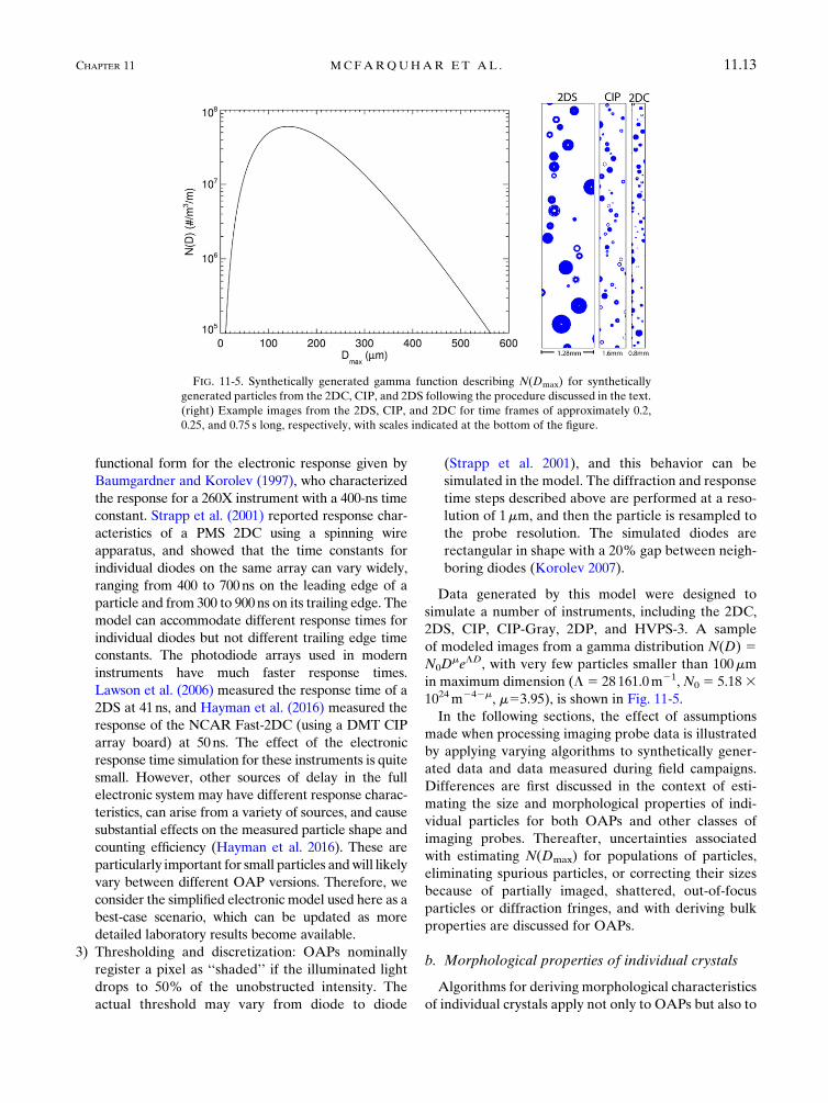
Data generated by this model were designed to

simulate a number of instruments, including the 2DC,

2DS, CIP, CIP-Gray, 2DP, and HVPS-3. A sample

of modeled images from a gamma distribution N(D) 5N0D

meLD, with very few particles smaller than 100mm

in maximum dimension (L 5 28 161.0m21, N0 5 5.1831024m242m, m53.95), is shown in Fig. 11-5.

In the following sections, the effect of assumptions

made when processing imaging probe data is illustrated

by applying varying algorithms to synthetically gener-

ated data and data measured during field campaigns.

Differences are first discussed in the context of esti-

mating the size and morphological properties of indi-

vidual particles for both OAPs and other classes of

imaging probes. Thereafter, uncertainties associated

with estimating N(Dmax) for populations of particles,

eliminating spurious particles, or correcting their sizes

because of partially imaged, shattered, out-of-focus

particles or diffraction fringes, and with deriving bulk

properties are discussed for OAPs.

b. Morphological properties of individual crystals

Algorithms for deriving morphological characteristics

of individual crystals apply not only to OAPs but also to

FIG. 11-5. Synthetically generated gamma function describing N(Dmax) for synthetically

generated particles from the 2DC, CIP, and 2DS following the procedure discussed in the text.

(right) Example images from the 2DS, CIP, and 2DC for time frames of approximately 0.2,

0.25, and 0.75 s long, respectively, with scales indicated at the bottom of the figure.

CHAPTER 11 MCFARQUHAR ET AL . 11.13

higher-resolution optical imagers. Typically analyzed

morphological properties of individual particles include

the maximum dimension Dmax, projected area Ap, pe-

rimeter Pp, and particle habit. Different algorithms used

to size particles are discussed by Korolev et al. (1998b),

Strapp et al. (2001), Lawson (2011), Brenguier et al.

(2013), and Wu and McFarquhar (2016) for mono-

chromatic OAPs; by Joe and List (1987) and Reuter and

Bakan (1998) for grayscale probes; and by Lawson et al.

(2001), Nousiainen and McFarquhar (2004), Baker and

Lawson (2006), and Um et al. (2015) for higher-

resolution imaging probes. In this subsection, the deri-

vation of ametric for particle size is first discussed. Then,

the use of a metric for particle morphology to derive

particle habit, as applicable to any category of particle

imager, is presented.

OAPs measure particles in two perpendicular di-

rections: the first aligned with the photodiode array

(widthWp) and the second along the direction of aircraft

motion (length Lp). This provides a two-dimensional

projection of a particle since the probe records the on/

off state of the diode array at each time interval that it

travels a distance of the size resolution. Alternate par-

ticle metrics, such as the maximum dimension in any

direction (Dmax) and area-equivalent diameter (Darea),

can also be derived.

There are several uncertainties associated with de-

riving particle size from OAP measurements. First,

when calculating Lp for legacy probes (i.e., those origi-

nally manufactured by PMS) some algorithms add an

additional slice to account for the one that is missed

waiting for the next clock cycle. The newer probes do

not skip the first slice, hence this correction is un-

necessary. Second, the meaning of Lp and Wp can be

ambiguous in the case of nonspherical particles, espe-

cially with gaps or holes (unshadowed diodes within the

image). These gaps or holes commonly occur when a

particle is imaged by an OAP far from the object plane

and is out of focus. The imaged particle gradually gets

larger as it moves farther from the object plane, and a

blank space can appear in its center as a result of the

diffraction effect (Poisson spot; see Fig. 6 in Korolev

2007). For out-of-focus droplets, Korolev (2007) shows

how the imaged size and Poisson spot diameter change

with distance from the object plane, and describes the

effect of digitization. Figure 11-6 illustrates examples of

two synthetically generated 200-mm out-of-focus parti-

cles and one in-focus particle as would be imaged by the

2DS, with estimates of Lp, Wp, Dmax, Pp, and Ap ob-

tained by different algorithms shown in Table 11-2.

Even before any corrections for out-of-focus particles

are applied there can be differences in how the size is

derived. For example, some algorithms calculate Lp and

Wp of the whole particle image, whereas others compute

them for the largest continuous part of the particle.

Differences for Lp, Wp, Dmax, Pp, and Ap estimated by

the University of Illinois/Oklahoma Optical Array

Probe Processing Software (UIOOPS) and the Univer-

sity of Manchester Optical Array Shadow Imaging

Software (OASIS) are 20% on average in Table 11-2

for the second particle in Fig. 11-6, but only 1.5% for the

first particle. The Rosenberg software has a range of

sizes as one of its inputs is the maximum distance be-

tween two shadowed pixel centers for them to be

counted as part of the same particle—the range repre-

sents setting this to either 1 or 128 pixels. The first par-

ticle represents the type of out-of-focus image that is

more commonly seen in OAPmeasurements. Given this

fact, it is not surprising that there was no significant

difference between estimates of Lp andWp by UIOOPS

and OASIS for 97.4% and 94.7% of all simulated

2DS particles. In-focus particles and varying degrees of

out-of-focus particles are included in the sample. There

are only differences in Lp and Wp when the particles

FIG. 11-6. Images of three 200-mm particles synthetically generated for a 2DS probe. Table 11-2 gives estimated Lp,Wp,Dmax, Pp, and

Ap from different processing algorithms for these 3 particles. The Z positions (relative to midpoint between the arms) of the particles are

21.4mm (particle 28), 24.2mm (particle 83), and 0.1mm (particle 517).

11.14 METEOROLOG ICAL MONOGRAPHS VOLUME 58

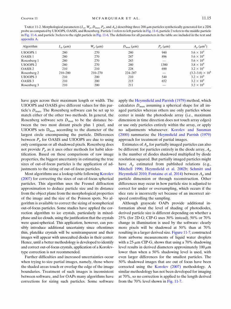
have gaps across their maximum length or width. The

UIOOPS and OASIS give different values for this par-

ticle’s Dmax. The Rosenberg software can be set up to

match either of the other two methods. In general, the

Rosenberg software sets Dmax to be the distance be-

tween the two most distant pixels plus 1 pixel, and

UIOOPS sets Dmax according to the diameter of the

largest circle encompassing the particle. Differences

between Pp for OASIS and UIOOPS are due to using

only contiguous or all shadowed pixels. Rosenberg does

not provide Pp as it uses other methods for habit iden-

tification. Based on these comparisons of raw image

properties, the biggest uncertainty in estimating the true

sizes of out-of-focus particles is the application of ad-

justments to the sizing of out-of-focus particles.

Most algorithms use a lookup table following Korolev

(2007) for correcting the sizes of out-of-focus spherical

particles. This algorithm uses the Fresnel diffraction

approximation to deduce particle size and its distance

from the object plane from themorphological properties

of the image and the size of the Poisson spots. No al-

gorithm is available to correct the sizing of nonspherical

out-of-focus particles. Some studies have applied the cor-

rection algorithm to ice crystals, particularly in mixed-

phase and ice clouds, using the justification that the crystals

were quasi-spherical. This application, however, can pos-

sibly introduce additional uncertainty since oftentimes

thin, platelike crystals will be semitransparent and their

images will appear with unocculted diodes in their center.

Hence, until a better methodology is developed to identify

and correct out-of-focus crystals, application of a Korolev-

type correction is not recommended.

Further difficulties and increased uncertainties occur

when trying to size partial images, namely, those where

the shaded areas touch or overlap the edge of the image

boundaries. Treatment of such images is inconsistent

between software, and for OAPs many algorithms have

corrections for sizing such particles. Some software

apply the Heymsfield and Parrish (1979) method, which

calculates Dmax assuming a spherical shape for all im-

aged particles whereas others use only particles whose

center is inside the photodiode array (i.e., maximum

dimension in time direction does not touch array edges)

or use only particles entirely within the array, or apply

no adjustments whatsoever. Korolev and Sussman

(2000) summarize the Heymsfield and Parrish (1979)

approach for treatment of partial images.

Estimates ofAp for partially imaged particles can also

be different: for particles entirely in the diode array, Ap

is the number of diodes shadowed multiplied by diode

resolution squared. But partially imaged particles might

have Ap estimated from published relations (e.g.,

Mitchell 1996; Heymsfield et al. 2002b; Schmitt and

Heymsfield 2010; Fontaine et al. 2014) between Ap and

particle dimension or through reconstruction. Other

differences may occur in how particle size is adjusted to

correct for under or oversampling, which occurs if the

slice rate is incorrectly set because of an incorrect air-

speed controlling the sampling.

Although grayscale OAPs provide additional in-

formation about the level of shading of photodiodes,

derived particle size is different depending on whether a

25% (for 2D-G; CIP-G uses 30% instead), 50% or 70%

change in illumination is used by the software: clearly

more pixels will be shadowed at 50% than at 70%

resulting in a larger derived size. Figure 11-7, constructed

from airborne measurements of liquid water droplets

with a 25-mm CIP-G, shows that using a 70% shadowing

level results in derived diameters approximately 100mm

lower than when a 50% shadowing level is used, with

even larger differences for the smallest particles. The

50% shadowed images that are out of focus have been

corrected using the Korolev (2007) methodology. A

similar methodology has not been developed for imaging

at 70%, so no correction is applied to the length derived

from the 70% level shown in Fig. 11-7.

TABLE 11-2. Morphological parameters (Lp,Wp,Dmax, Pp, andAp) describing three 200-mm particles synthetically generated for a 2DS

probe as computed byUIOOPS,OASIS, andRosenberg. Particle 1 refers to left particle in Fig. 11-6, particle 2 refers to themiddle particle

in Fig. 11-6, and particle 3refers to the right particle in Fig. 11-6. The definitions for all parameters in the table are included in the text and

appendix A.

Algorithm Lp (mm) Wp (mm) Dmax (mm) Pp (mm) Ap (mm2)

UIOOPS 1 280 270 280 940 5.6 3 104

OASIS 1 280 270 287 896 5.6 3 104

Rosenberg 1 280 270 283 — 5.6 3 104

UIOOPS 2 280 270 280 1380 3.8 3 104

OASIS 2 210 210 228 690 3.2 3 104

Rosenberg 2 210–280 210–270 224–287 — (3.2–3.8) 3 104

UIOOPS 3 210 200 210 540 3.2 3 104

OASIS 3 210 200 215 652 3.2 3 104

Rosenberg 3 210 200 211 — 3.2 3 104

CHAPTER 11 MCFARQUHAR ET AL . 11.15

There are several different ways in whichDmax can be

defined (Battaglia et al. 2010; Lawson 2011; Brenguier

et al. 2013; Wood et al. 2013) for cloud particle images.

Wu and McFarquhar (2016) evaluated six commonly

used definitions of Dmax for ice clouds: 1) maximum

dimension in the time direction Lp; 2) maximum di-

mension in the photodiode array direction Wp; 3) the

larger of Lp and Wp (DL); 4) the mean of Lp and

Wp (DA); 5) the hypotenuse of a right-angled triangle

constructed from Lp and Wp (DH); and 6) the diameter

of the smallest circle enclosing particle DS. The eval-

uation focused on how the application of these six

definitions affected N(Dmax) for OAPs. As shown in

Fig. 11-8, N(Dmax) can differ by up to a factor of 6. It

should be noted that for liquid or nearly spherical par-

ticles each of these definitions should yield a similar

value. However, for other particles significant differ-

ences are expected and it is not always clear which

definition is closest to Dmax because a two-dimensional

shadow of a three-dimensional particle with arbitrary

orientation with respect to the optical plane is seen. Ice

particles withD. 100mm have preferential orientation

while falling in air (Pruppacher and Klett 1997) so that

particles imaged by probes with a vertical orientation of

the laser beam have silhouettes with close to the maxi-

mum particle projection. FollowingUm andMcFarquhar

(2007), an iterative procedure for pristine, regular particle

shapes can be followed to estimate the three-dimensional

size, but this still does not represent a direct measure in

three dimensions.

Varying measures of particle morphology (Lp, Wp,

Dmax, Ap, Pp, etc.) are also used to identify particle

habits using a number of classification schemes. In ad-

dition to manual classification, such schemes have used

morphological measures of crystals (e.g., Holroyd 1987;

Um and McFarquhar 2009, hereinafter UM09), neural

networks (McFarquhar et al. 1999), pattern recognition

techniques (Duroure 1982; Moss and Johnson 1994),

dimensionless ratios of geometrical measures (Korolev

and Sussman 2000), principal component analysis

(Lindqvist et al. 2012), characteristic positions of trig-

gered pixels (Fouilloux et al. 1997), and Fourier analysis

(Hunter et al. 1984) to assign shapes. These habit clas-

sification schemes have been developed and imple-

mented for OAPs and other cloud imagers.

Uncertainties associated with such schemes are illus-

trated using data collected by a cloud particle imager

(CPI) during the Tropical Warm Pool International

Cloud Experiment (May et al. 2008) and the Indirect

and Semi-Direct Aerosol Campaign (McFarquhar et al.

2011b). Data from the CPI are used because it has

higher-resolution than the OAPs and hence allows an

assessment of how the methodology itself, rather than

the limited resolution of images, affects the identifica-

tion of shape. Figure 11-9 shows inferred habit distri-

butions based on the UM09 algorithm and the SPEC

CPIView software (SPEC 2012). Large differences in

habit definition evident in this figure are caused by a

number of factors. First, there is ambiguity in the defi-

nition of habit categories. Although several categories

are common (i.e., column, plate, and bullet rosette),

other categories differ (e.g., bullet rosettes, aggregates,

and irregulars). The number of categories also differs,

with manual classifications (e.g., Magono and Lee 1966;

Katsuhiro et al. 2013) typically having more categories

than shown in Fig. 11-9. In general, the fraction of

pristine crystals (i.e., column and bullet rosettes) iden-

tified by different methods are comparable, while those

for nonpristine or irregular crystals, which frequently

dominate habits (e.g., Korolev et al. 1999; Um et al.

2015), are not. Morphological measures of particles

(e.g., Lp,Wp,Dmax, Ap, and Pp) can differ depending on

the threshold values used to extract them (Korolev and

Isaac 2003).

Similar schemes can be applied to OAPs, with their

applicability depending somewhat on the resolution of

the sensor. In some studies, such as Jackson et al. (2012),

habit-dependent size distributions are generated by

applying the fraction of size-dependent, identified habits

(by the CPI) to size distributions measured by OAPs.

This approach takes advantage of the higher resolution

of the CPI complemented by the larger and more well-

defined sample volume of the OAP.

FIG. 11-7. Relationship between particle length determined from

a gray probe depending upon whether 70% or 50% shadowing was

used to define the particles. This comparison was constructed from

water droplets measured with an airborne CIP-Gray probe. The

embedded filmstrip shows representative particles that were im-

aged by the probe for the time period analyzed.

11.16 METEOROLOG ICAL MONOGRAPHS VOLUME 58

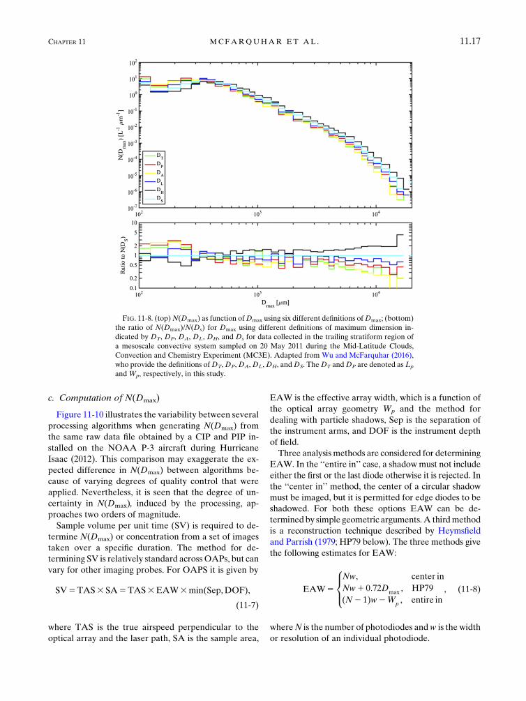
c. Computation of N(Dmax)

Figure 11-10 illustrates the variability between several

processing algorithms when generating N(Dmax) from

the same raw data file obtained by a CIP and PIP in-

stalled on the NOAA P-3 aircraft during Hurricane

Isaac (2012). This comparison may exaggerate the ex-

pected difference in N(Dmax) between algorithms be-

cause of varying degrees of quality control that were

applied. Nevertheless, it is seen that the degree of un-

certainty in N(Dmax), induced by the processing, ap-

proaches two orders of magnitude.

Sample volume per unit time (SV) is required to de-

termine N(Dmax) or concentration from a set of images

taken over a specific duration. The method for de-

termining SV is relatively standard acrossOAPs, but can

vary for other imaging probes. For OAPS it is given by

SV5TAS3SA5TAS3EAW3min(Sep,DOF),

(11-7)

where TAS is the true airspeed perpendicular to the

optical array and the laser path, SA is the sample area,

EAW is the effective array width, which is a function of

the optical array geometry Wp and the method for

dealing with particle shadows, Sep is the separation of

the instrument arms, and DOF is the instrument depth

of field.

Three analysismethods are considered for determining

EAW. In the ‘‘entire in’’ case, a shadowmust not include

either the first or the last diode otherwise it is rejected. In

the ‘‘center in’’ method, the center of a circular shadow

must be imaged, but it is permitted for edge diodes to be

shadowed. For both these options EAW can be de-

terminedby simple geometric arguments.A thirdmethod

is a reconstruction technique described by Heymsfield

and Parrish (1979; HP79 below). The three methods give

the following estimates for EAW:

EAW5

8><>:Nw, center in

Nw1 0:72Dmax

, HP79

(N2 1)w2Wp, entire in

, (11-8)

whereN is the number of photodiodes andw is the width

or resolution of an individual photodiode.

FIG. 11-8. (top)N(Dmax) as function ofDmax using six different definitions ofDmax; (bottom)

the ratio of N(Dmax)/N(Ds) for Dmax using different definitions of maximum dimension in-

dicated by DT, DP, DA, DL, DH, and Ds for data collected in the trailing stratiform region of

a mesoscale convective system sampled on 20 May 2011 during the Mid-Latitude Clouds,

Convection and Chemistry Experiment (MC3E). Adapted from Wu and McFarquhar (2016),

who provide the definitions ofDT,DP,DA,DL,DH, andDS. TheDT andDP are denoted as Lp

and Wp, respectively, in this study.

CHAPTER 11 MCFARQUHAR ET AL . 11.17

TheDOF is defined by the diffraction of the light by the

measured particle. Particles farther from the optical plane

cause less deep shadows until eventually they do not

shadow any photodiodes above the required amount for

detection. The distance between points on either side of

the optical plane where particles disappear defines the

DOF, which is double the distance a particle can be from

the object plane and still shadow a photodiode by the ap-

propriate preset threshold. As was shown experimentally

by Knollenberg (1970) and then analytically by Korolev

et al. (1998b) the diffraction pattern of a spherical particle

is a function of the dimensionless parameterZd5 lljZj/R2,

with Z the distance between the particle and object plane,

ll the laser wavelength and R the particle radius, which

would be Dmax/2 for spherical particles. The implications

for nonspherical particles are discussed below.

Thus, the DOF is typically represented as 2gR2/llwith

the DOF’s maximum value set by the distance between

FIG. 11-9. Habit fraction by number for 30-s time intervals produced from different algorithms

[UM09 and SPEC CPIView (SPEC)] for ice crystals with Dmax . 50mm imaged by CPI during

the (top) Tropical Warm Pool International Cloud Experiment (TWP-ICE) and (bottom) In-

direct and Semi-Direct Aerosol Campaign (ISDAC). UM09 has 12 habits: small- (SQ), medium-

(MQ), and large-quasi sphere (LQ), plate (PLT), aggregates of plates (APs), bullet rosette (BR),

aggregates of bullet rosettes (ABRs), column (COL), aggregates of columns (ACs), dendrite

(DEN), capped column (CC), and unclassified (UC). SPEC has 7 habits: spheroid (SPR), PLT,

rosette (ROS), COL, budding rosette (BROS), small irregular (SIR), and big irregular (BIR).

11.18 METEOROLOG ICAL MONOGRAPHS VOLUME 58

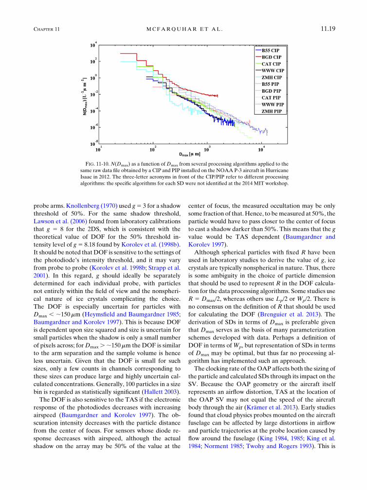
probe arms. Knollenberg (1970) used g5 3 for a shadow

threshold of 50%. For the same shadow threshold,

Lawson et al. (2006) found from laboratory calibrations

that g 5 8 for the 2DS, which is consistent with the

theoretical value of DOF for the 50% threshold in-

tensity level of g5 8.18 found by Korolev et al. (1998b).

It should be noted thatDOF is sensitive to the settings of

the photodiode’s intensity threshold, and it may vary

from probe to probe (Korolev et al. 1998b; Strapp et al.

2001). In this regard, g should ideally be separately

determined for each individual probe, with particles

not entirely within the field of view and the nonspheri-

cal nature of ice crystals complicating the choice.

The DOF is especially uncertain for particles with

Dmax , ;150mm (Heymsfield and Baumgardner 1985;

Baumgardner and Korolev 1997). This is because DOF

is dependent upon size squared and size is uncertain for

small particles when the shadow is only a small number

of pixels across; forDmax.;150mm the DOF is similar

to the arm separation and the sample volume is hence

less uncertain. Given that the DOF is small for such

sizes, only a few counts in channels corresponding to

these sizes can produce large and highly uncertain cal-

culated concentrations. Generally, 100 particles in a size

bin is regarded as statistically significant (Hallett 2003).

The DOF is also sensitive to the TAS if the electronic

response of the photodiodes decreases with increasing

airspeed (Baumgardner and Korolev 1997). The ob-

scuration intensity decreases with the particle distance

from the center of focus. For sensors whose diode re-

sponse decreases with airspeed, although the actual

shadow on the array may be 50% of the value at the

center of focus, the measured occultation may be only

some fraction of that. Hence, to bemeasured at 50%, the

particle would have to pass closer to the center of focus

to cast a shadow darker than 50%. This means that the g

value would be TAS dependent (Baumgardner and

Korolev 1997).

Although spherical particles with fixed R have been

used in laboratory studies to derive the value of g, ice

crystals are typically nonspherical in nature. Thus, there

is some ambiguity in the choice of particle dimension

that should be used to represent R in the DOF calcula-

tion for the data processing algorithms. Some studies use

R 5 Dmax/2, whereas others use Lp/2 or Wp/2. There is

no consensus on the definition of R that should be used

for calculating the DOF (Brenguier et al. 2013). The

derivation of SDs in terms of Dmax is preferable given

that Dmax serves as the basis of many parameterization

schemes developed with data. Perhaps a definition of

DOF in terms ofWp, but representation of SDs in terms

of Dmax may be optimal, but thus far no processing al-

gorithm has implemented such an approach.

The clocking rate of theOAP affects both the sizing of

the particle and calculated SDs through its impact on the

SV. Because the OAP geometry or the aircraft itself

represents an airflow distortion, TAS at the location of

the OAP SV may not equal the speed of the aircraft

body through the air (Krämer et al. 2013). Early studies

found that cloud physics probes mounted on the aircraft

fuselage can be affected by large distortions in airflow

and particle trajectories at the probe location caused by

flow around the fuselage (King 1984, 1985; King et al.

1984; Norment 1985; Twohy and Rogers 1993). This is

FIG. 11-10.N(Dmax) as a function ofDmax from several processing algorithms applied to the

same raw data file obtained by a CIP and PIP installed on the NOAAP-3 aircraft in Hurricane

Isaac in 2012. The three-letter acronyms in front of the CIP/PIP refer to different processing

algorithms: the specific algorithms for each SD were not identified at the 2014 MIT workshop.

CHAPTER 11 MCFARQUHAR ET AL . 11.19

further discussed in chapter 9 (Baumgardner et al. 2017)

in section 6 under the subheading ‘‘Impact of mounting

location.’’ Most OAP probes are now mounted in select

locations below the aircraft wing, where distortions due

to the aircraft itself are usually smaller. However, local

distortions in TAS and flow angle are still possible be-

cause of varying airflow about the wing, through the

OAP arms, or compression upstream of the housing it-

self (Norment 1988; Weigel et al. 2016). A bias in a local

static reference point due to slowing airflow can have a

large impact on the calculated TAS. Computational

fluid dynamics studies and empirical corrections are

useful for handling these effects (Weigel et al. 2016). In

addition, a simple method of adjusting image aspect

ratios to expected values can be used if preferentially

oriented crystals are not present (King 1984, 1985; King

et al. 1984).

For legacy probes, particle images are typically

stored in two buffers so that one can be used to store

images when data from the other are transmitted to the

data system. But, in clouds with high concentrations,

the second buffer can fill up while the first is still

transmitting. In this case, there will be a dead period

when no data are recorded. For some newer probes

(e.g., the 2DS), the probes skip individual particles in

overload and keep track of the dead time so that the

sample volume can be corrected. Other probes, such as

the CIP and PIP, have a counter that keeps track of

skipped particles so that SDs can be reconstructed.

However, when the CIP buffers are full, only the

number of particles and Wp are recorded without tim-

ing information. This means that during overload pe-

riods it is difficult to make corrections for shattered

particles (see below). In any event, checks should en-

sure that the sum of particle interarrival times matches

the record time to insure the timing information is

correctly recorded. Implementation of such corrections

in different algorithms may cause discrepancies in the

derived N(Dmax).

d. Removal of spurious particles

Additional algorithms are applied to remove artifacts

from the measured data. As discussed in chapter 9

(Baumgardner et al. 2017), small crystals can be gener-

ated from the shattering of larger crystals on the pro-

truding tips and inlets of probes. These do not represent

naturally occurring crystals. There are algorithms that

attempt to eliminate shattering artifact particles based

on the time between particle arrivals in the sample

volume (Cooper 1978; Field et al. 2003, 2006) (i.e., in-

terarrival time ti), and on the numbers, sizes, and gaps

between fragments in a single image (Korolev and Isaac

2005). Further elaboration and analysis of limitations of

the interarrival time algorithmwas described in Korolev

and Field (2015). Many studies have implemented such

algorithms (e.g., Baker et al. 2009; Korolev et al. 2011,

2013c; Lawson 2011; Jackson et al. 2014).

The basis of interarrival time algorithms (e.g., Field

et al. 2006; Baker et al. 2009; Lawson 2011; Korolev

et al. 2011, 2013b; Jackson et al. 2014) is that a bimodal

Poisson probability density function describes the dis-

tribution of ti, where particles occurring in a peak

with a larger mode t1 correspond to naturally occurring

particles and those in a peak with a smaller mode t2correspond to potentially shattered particles. Figure 11-11

shows a distribution of interarrival times measured by

a 2DS probe installed on the French Falcon aircraft

during the collaborative 2014 European High Altitude

Ice Crystals and the North American High Ice Water

Content projects (HAIC/HIWC); similar figures showing

distributions of interarrival times or distances are found

in Lawson (2011), Korolev et al. (2011, 2013b), Jackson

et al. (2014) and others. The peak at an interarrival time

of 6 3 1024 s corresponds to naturally occurring parti-

cles, whereas the peak at an interarrival time less than

1026 s corresponds to shattered artifacts. Generally

there may be some overlap between the two modes and

different approaches exist for choosing a threshold ti so

that few naturally occurring particles are removed and

most artifacts are removed.

Examples of different approaches for making inter-

arrival time corrections are illustrated in Fig. 11-12,

which shows the frequency distribution of interarrival

times recorded by the 2DS during HAIC/HIWC as a

function of time. The different colored lines show how

FIG. 11-11. Normalized frequency distribution of interarrival

times recorded by a 2DS probe installed on a French Falcon air-

craft during the collaborative 2014HAIC/HIWC project on 18 Feb

2014. Solid lines represent best fits to modes of peaks describing

naturally occurring particles and shattered artifacts, generated

following approach of Jackson et al. (2014).

11.20 METEOROLOG ICAL MONOGRAPHS VOLUME 58

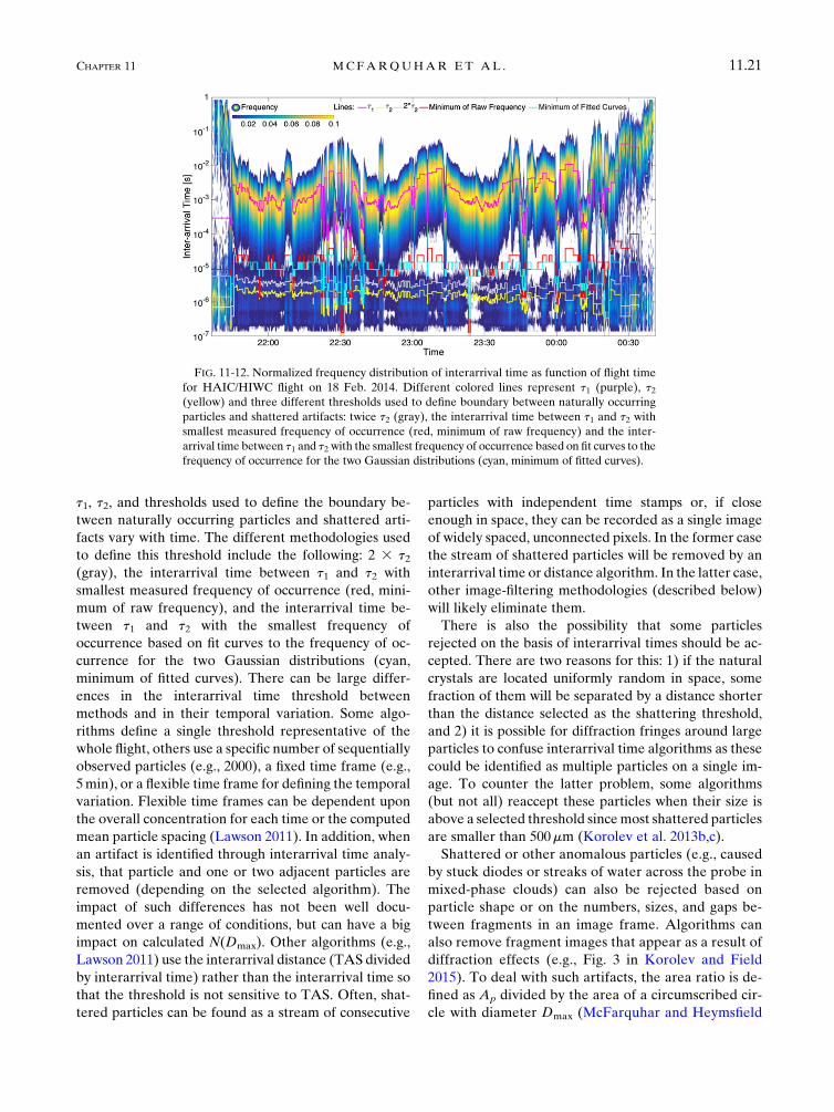
t1, t2, and thresholds used to define the boundary be-

tween naturally occurring particles and shattered arti-

facts vary with time. The different methodologies used

to define this threshold include the following: 2 3 t2(gray), the interarrival time between t1 and t2 with

smallest measured frequency of occurrence (red, mini-

mum of raw frequency), and the interarrival time be-

tween t1 and t2 with the smallest frequency of

occurrence based on fit curves to the frequency of oc-

currence for the two Gaussian distributions (cyan,

minimum of fitted curves). There can be large differ-

ences in the interarrival time threshold between

methods and in their temporal variation. Some algo-

rithms define a single threshold representative of the

whole flight, others use a specific number of sequentially

observed particles (e.g., 2000), a fixed time frame (e.g.,

5min), or a flexible time frame for defining the temporal

variation. Flexible time frames can be dependent upon

the overall concentration for each time or the computed

mean particle spacing (Lawson 2011). In addition, when

an artifact is identified through interarrival time analy-

sis, that particle and one or two adjacent particles are

removed (depending on the selected algorithm). The

impact of such differences has not been well docu-

mented over a range of conditions, but can have a big

impact on calculated N(Dmax). Other algorithms (e.g.,

Lawson 2011) use the interarrival distance (TAS divided

by interarrival time) rather than the interarrival time so

that the threshold is not sensitive to TAS. Often, shat-

tered particles can be found as a stream of consecutive

particles with independent time stamps or, if close

enough in space, they can be recorded as a single image

of widely spaced, unconnected pixels. In the former case

the stream of shattered particles will be removed by an

interarrival time or distance algorithm. In the latter case,

other image-filtering methodologies (described below)

will likely eliminate them.

There is also the possibility that some particles

rejected on the basis of interarrival times should be ac-

cepted. There are two reasons for this: 1) if the natural

crystals are located uniformly random in space, some

fraction of them will be separated by a distance shorter

than the distance selected as the shattering threshold,

and 2) it is possible for diffraction fringes around large

particles to confuse interarrival time algorithms as these

could be identified as multiple particles on a single im-

age. To counter the latter problem, some algorithms

(but not all) reaccept these particles when their size is

above a selected threshold sincemost shattered particles

are smaller than 500mm (Korolev et al. 2013b,c).

Shattered or other anomalous particles (e.g., caused

by stuck diodes or streaks of water across the probe in

mixed-phase clouds) can also be rejected based on

particle shape or on the numbers, sizes, and gaps be-

tween fragments in an image frame. Algorithms can

also remove fragment images that appear as a result of

diffraction effects (e.g., Fig. 3 in Korolev and Field

2015). To deal with such artifacts, the area ratio is de-

fined as Ap divided by the area of a circumscribed cir-

cle with diameter Dmax (McFarquhar and Heymsfield

FIG. 11-12. Normalized frequency distribution of interarrival time as function of flight time

for HAIC/HIWC flight on 18 Feb. 2014. Different colored lines represent t1 (purple), t2(yellow) and three different thresholds used to define boundary between naturally occurring

particles and shattered artifacts: twice t2 (gray), the interarrival time between t1 and t2 with

smallest measured frequency of occurrence (red, minimum of raw frequency) and the inter-

arrival time between t1 and t2 with the smallest frequency of occurrence based on fit curves to the

frequency of occurrence for the two Gaussian distributions (cyan, minimum of fitted curves).

CHAPTER 11 MCFARQUHAR ET AL . 11.21

1996). Particles with area ratios less than 0.1 or 0.2 are

commonly identified as artifacts. It is worth noting

that there is little consistency between algorithms in

how/if shatter artifacts, diffraction fringe artifacts,

and other image artifacts are dealt with. These dif-

ferences contribute to variations in the subsequently

derived N(Dmax).

e. Derivation of bulk properties

Based on the derived N(Dmax), a number of bulk

cloud microphysical properties related to various mo-

ments of the distribution can be derived where

Mn5

ðD1

D0

N(Dmax

)Dnmax dDmax

, (11-9)

where Mn is the nth moment of the distribution, and D0

and D1 are the minimum and maximum diameters over

which N(Dmax) was measured. Thus, the total number

concentration is M0 and wi 5 aMb when the mass of an

individual ice particle is represented as aDbmax, where

a and b are habit-dependent coefficients (Locatelli and

Hobbs 1974; Mitchell 1996). Higher-order moments can

also be represented in terms of othermeasures of particle

morphology, such as Baker and Lawson’s (2006) calcu-

lation of particle mass in terms of projected area. Un-

certainties in derived bulk properties are dependent

upon uncertainties in N(Dmax) and the applicability of

the relevant algorithm used to define properties of indi-

vidual particles. For example, Field et al. (2006) and

Jackson and McFarquhar (2014) found small crystal ar-

tifacts produced by shattering make estimates in total

concentration highly uncertain because the zeroth-order

moment is highly dependent on concentrations of parti-

cles with Dmax , 500mm, namely, those particles pro-

duced by shattering. But, estimates ofwi had atmost 20%

uncertainty from shattering because its higher-order

moment is more dominated by larger particles not gen-

erated by shattering; in fact, uncertainties associated with

estimating a three-dimensional shape and density from a

two-dimensional image are larger.

Derived bulk properties are sensitive to the definition

of Dmax (Wu and McFarquhar 2016). For instance, Dm

can vary by 2 times, wi as much as 3 times, and b up to 2

times, depending on the definition used.

f. Processing, analysis, and presentation software

A number of different software packages are used for

processing, analyzing, and presenting data from cloud

probes. In this section, a path forward is discussed for

creating community-based open-source software that will

make differences in processing algorithms more trans-

parent. Since themost complex processing algorithms are

for data collected by OAPs, this section concentrates on

code that processes these types of spectrometers.

Available processing codes for OAPs include the

System for OAP Data Analysis (SODA) developed at

NCAR; OASIS; UIOOPS; the Airborne Data Process-

ing andAnalysis (ADPAA) developed at theUniversity

of North Dakota, the Software for Airborne Measure-

ments of Aerosols and Clouds (SAMAC; Gagne et al.

2016); and software packages developed at SPEC Inc.,

Environment and Climate Change Canada, and Leeds

University (Rosenberg software referenced previously).

Although there are differences between codes with re-

spect to the programming language, platforms sup-

ported, and algorithms by which data are processed,

there are also many common features: all algorithms

convert raw measurements into single-particle data that

are used to derive SDs and bulk cloud properties.

Because there are many different codes for processing

data from OAPs and the inherent algorithms and codes

may change occasionally, a detailed discussion of the

individual algorithms is not provided here. However, it

is noted that most codes can handle data from a variety

of data acquisition systems, raw data formats, and

buffering schemes. Morphological measures of the de-

rived single-particle properties typically include various

properties that could be used to define Dmax (e.g., the

diameter of the minimum enclosing circle, or maximum

length in the photodiode or time array), projected area,

aspect ratio (Korolev and Isaac 2003), particle habit,

and a measure of the complexity of the image. Correc-

tions are applied for out-of-focus, undersampled, or

partially imaged particles and for diffraction (e.g.,

Korolev 2007), and particles are rejected depending on

image shapes (aspect or area ratio), interarrival time or

spacing distance (e.g., Field et al. 2006) or particle center

located outside the photodiode array. The N(Dmax) and

bulk properties are then determined using the size-

dependent sample volume. Many codes also provide

utilities for data display and visualization, computation

of derived bulk quantities, merging probes with different

size ranges, and data export. Codes may or may not

include a graphical interface.

Currently, distribution of OAP processing codes is com-

plicated because they are continually undergoing changes

as new algorithms are introduced or old ones edited. In

addition, as new instruments come on line, changes are

needed in existing codes to accommodate them. Further-

more, changes in the codes sometimes are necessary when

processing data from a different version of the same probe,

or more sophisticated tuning is mandated when processing

data from the same probe used in different conditions.

Therefore, it is a challenge for investigators who are not

code developers to grasp to grasp the sensitivity of derived

11.22 METEOROLOG ICAL MONOGRAPHS VOLUME 58

products to the assumptions that were used to process the

measurements. Hence, developers are reluctant to freely

distribute their software without associated caveats. Even

if a community code is developed, it will require continual

updates and modifications.

Many of these issues were discussed at the 2016

EUFAR International Commission on Clouds and Pre-

cipitation (ICCP) workshop on data processing, analysis,

and presentation software of cloud probes at the Uni-

versity of Manchester. Although consensus was not

reached by the participants on the optimum procedures

for processing cloud probe data, it was unanimous that

the need is urgent for a common reference library, in-

cluding the individual processing algorithms. For in-

clusion in this library, algorithms or software packages

should either have been published in the refereed litera-

ture or have passed through amutually agreed upon, peer

reviewed, internal vetting process. The need for using

some form of version control, the strong desire for open-

source software, and the recommendation of assigning a

digital object identifier (DOI) for individual processing

algorithms was also emphasized. However, given the

dynamic nature of the codes it may prove difficult to

assign a DOI to such codes. Hence, some other approach

for referencing and making codes available may be re-

quired. The availability of synthetic datasets and bench-

mark cases for evaluating new algorithms was also noted

as another critical component for evaluating new or

updated algorithms. The need for future workshops to

continue these collaborations was also aknowledged.

5. Future efforts

Since the development of cloud probes more than

50 years ago, processing algorithms have been developed

to derive single-particle properties, size distributions,

and bulk parameters for ice clouds. Significant progress

has been made in understanding the basic sensing prin-

ciples and inherent measurement uncertainties that have

led to correction algorithms for issues such as conduction

and convection from a heated wire to the surrounding

cold air. While adjustments to concentration data are

well known and documented for scattering probes, the

sizing of ice crystals is less certain. Artifical shattering of

ice crystals is a problem for both light-scattering spec-

trometers and particle-imaging probes, but antishatter-

ing tips and spurious particle removal algorithms have

helped correct for this issue. In addition to shattering,

concentration data from particle-imaging probes can be

greatly affected by numerous other issues including

maximum dimension definition, depth of field calcula-

tion, effective array width choice, image diffraction, and

true airspeed assumption. The details and assumptions in

some of these processing algorithms can have large ef-

fects on the derived cloud products. With the application

of various codes by different groups and no clear con-

sensus on the optimal methodology for processing data,

it remains a challenge to compare data processed by

different groups, or sometimes even by the same group,

from different field campaigns. In addition, the specific

calibration for individual probes may not be known

or available so that differences in calibrations can in-

troduce additional uncertainties. Further, the exact set

of assumptions used to process data from a particular

field project is not always clear, and even if such as-

sumptions were well documented, their effect on derived

properties is not well known. Therefore, it is difficult to

make progress on understanding how cloud properties

vary with geographical location and environmental

conditions, a prerequisite for understanding cloud pro-

cesses and improving the representation of these pro-

cesses in weather and climate models.

Processing algorithms for interpreting data from total

water content and forward-scattering probes are more

mature than for those for imaging probes. For heated

sensors, estimating the dry-air term and removing base-

line offsets are the largest uncertainties. For total water

content probes that vaporize cloud droplets and ice

crystals, removing the baseline offset, estimating particle

cut sizes from the counterflow, and determining the im-

portance of particles bouncing out of the sensor volume

are the biggest unknowns. For forward-scattering probes,

coincidence and shattering adjustments, calibration of bin

boundaries to account for oscillations in instrument re-

sponse, and sizing nonspherical ice crystals are the largest

uncertainties. Ongoing efforts to intercompare algo-

rithms in water clouds improve our understanding of how

algorithms perform in ice because closure studies are

simpler in the presence of spherical water drops.

Uncertainties in processing image probe data and dis-

crepancies between processing codes are especially preva-

lent. To reduce the uncertainties associated with processing

of measurements and to make assumptions used in pro-

cessing data more transparent, more methodical algorithm

comparisons are needed. In particular, a raw or synthetic

data file (i.e., a benchmark) should be processed by several

groups in sequential steps. For example, raw counts as a

function of size for complete, partial and total images

should be compared before comparing derived SDs.

Thereafter particular image correction techniques (e.g.,

particle reconstruction, corrections for out-of-focus par-

ticles) and particle rejection algorithms should be se-

quentially activated in each code, with results compared

after each step. This will identify sources of discrepancies

in algorithms and show how different assumptions affect

and lead to uncertainty in derived products. Furthermore,

CHAPTER 11 MCFARQUHAR ET AL . 11.23

this should help establish best practices for processingOAP

data that could be widely adopted by different groups.

Other specific recommendations for OAPs include the

following:

1) Evaluation of grayscale probes to see if a better

definition of the DOF is possible;

2) further investigations of the nature of the DOF,

including its dependence on size and determining

if a definition better than 2gR2/ll is possible;

3) applications of consistency checks on collected data-

sets, such as determining if all diodes in the array

have uniform responses throughout the experiment;

4) closure tests to check that the sum of all channels in

the recorded 1-Hz distributions is equal to those

determined from the individual image counts.

Table 4.1 of Isaac and Schmidt (2009) lists possible ac-

curacies of different parameters derived from in situ sen-

sors. Chapter 9 (Baumgardner et al. 2017) of this

monograph is focused on instrument limitations and

measurement uncertainties and updates the Isaac and

Schmidt (2009) information to give quantitative un-

certainties in total water content and light-scattering and

imaging probes associated with the measurement tech-

niques themselves. In this paper, no attempt has been

made to quantitatively summarize the accuracy of quan-

tities derived from the processing algorithms. Despite

significant progress in the past 10 years, the development

and interpretation of processing techniques has revealed

more issues thatwere not previously recognized or thought

to be important (e.g., ice shattering, local airspeed in

probes’ sample areas, ice bouncing on hot wires, and par-

ticle reacceptance in processing software). This new

knowledge gives a retrospective on the quality of past as-

sessments of measurement accuracy, and some new esti-

mates of accuracy have been increased compared to past

estimates.Many of the errors are nonlinear and depend on

the value of themeasured parameter, and hence cannot be

easily summarized in a table. One of the biggest obstacles

hindering progress in understanding accuracy is the ab-

sence of measurement standards for particle concentra-

tion, ice water content, and ambiguity in sizing of

nonspherical particles. Thus, presenting a summary table

on instrument accuracy would be premature.

In addition, it is necessary for the community to develop

a strategy toward a consensus as to which assumptions are

optimal when processing in situ data from heated sensors

and forward-scattering and imaging probes. A community

workshop, a community survey, and code comparisons

would be beneficial in making these recommendations.

However, there cannot be a stagnant code or a frozen best

approach for processing data: inevitably the optimum al-

gorithmswill evolve over time asmore is learned about the

performance of the various probes and more sophisticated

algorithms are introduced and evaluated. Thus, all pro-

cessing codes should be open source, version controlled,

and well documented, preferentially with a DOI, even

though this is difficult with dynamic codes. With this ap-

proach, both code developers and data users are equally

able to processmicrophysical probe data. Finally, given the

agreement that all algorithms should be either published or

approved by a panel of experts, it may be appropriate for a

governing body or organizing entity to make recommen-

dations for best practices.

Ultimately, it would be of general benefit to develop a

community software package that incorporates different

algorithms and assumptions for processing the data (e.g.,

different algorithms for correcting out-of-focus particles

or rejecting shattered artifacts for imaging probes).

Examples and tutorials should be available to expand

the range of code users. Similar approaches have been

followed for the development of both weather and re-

search forecasting models (e.g., Skamarock et al. 2008)

and for theweather radar community (e.g., Heistermann

et al. 2015). Thirty or more years ago, all algorithms

would have been programmed in FORTRAN; with the

current existence of algorithms in many languages, code

sharing has become more difficult, so adopting a com-

munity programming language could also be beneficial.

Following the weather radar community, the Python

programming language is an attractive candidate for

such a package. In any event, the chosen package should

be modular so various authors can incorporate en-

hanced features or extra options as the community’s

knowledge evolves. It should also be recognized that the

development and maintenance of a common processing

capability requires resources that are currently not

available to any one group, and needs continual main-

tenance in order to be successful.

In summary, in situ measurements of cloud micro-

physical properties will remain critical for enhancing

process-oriented understanding of clouds, for evaluating

models and remote sensing retrievals, and for de-

veloping parameterizations for such models and re-

trievals in the foreseeable future. Although there will

always be uncertainties associated with the conversion

of raw data to geophysical variables, it is important that

future efforts minimize the uncertainties and thoroughly

document the assumptions used to obtain those vari-

ables so that it is possible to compare data obtained by

different groups in a wide range of projects in different

geophysical conditions.

Acknowledgments. This research was partially sup-

ported by the Office of Science (BER), United States

DOE under Grant DE-SC0014065, by the National

11.24 METEOROLOG ICAL MONOGRAPHS VOLUME 58

Science Foundation (NSF) under Grants AGS-1213311

and AGS-1359098, and by the DACCIWA project, which

has received funding from the European Union Seventh

Framework Programme (FP7/2007-2013) under Grant

Agreement 603502. The lead author was partially sup-

ported by an Advanced Study Program (ASP) visiting

faculty fellowship at NCAR during the writing of the

manuscript. The comments of seven anonymous reviewers

helped clarify the manuscript. The authors would like to

thank the many sponsors who have provided funding for

the monograph: Leibniz Institute for Tropospheric Re-

search (TROPOS), Forschungszentrum Jülich (FZJ), and

Deutsches Zentrum für Luft- und Raumfahrt (DLR),

Germany; ETH Zurich, Switzerland; National Center for

Atmospheric Research (NCAR), United States; the Met

Office, United Kingdom; the University of Illinois, United

States; Environment and Climate Change Canada

(ECCC), Canada; National Science Foundation (NSF),

AGS 1723548, National Aeronautics and Space Ad-

ministration (NASA), United States; the International

Commission on Clouds and Precipitation (ICCP), the

European Facility for Airborne Research (EUFAR),

and Droplet Measurement Technologies (DMT),

United States. NCAR is sponsored by the NSF. Any

opinions, findings, and conclusions or recommenda-

tions expressed in this publication are those of the

author(s) and do not necessarily reflect the views of the

National Science Foundation.

APPENDIX A

List of Symbols

A Habit-dependent coefficient used in m–

Dmax relations

ADOF Area corresponding to particles in depth

of field

Ap Projected area of particle

a1 Coefficient used to characterize base line

drift of Nevzorov probe

a2 Coefficient used to characterize base line

drift of Nevzorov probe

b Habit-dependent coefficient used in m–

Dmax relations

b0 Fit parameter established in wind tunnel test

or flight measurement

b1 Coefficient used to characterize base line

drift of Nevzorov probe

b2 Coefficient used to characterize base line

drift of Nevzorov probe

b3 Coefficient used to characterize base line

drift of Nevzorov probe

c Specific heat of water

Cf Adjustment factor for forward-scattering

probes

D Diameter of cylinder

DA Mean of Lp and Wp

Darea Area-equivalent diameter

DH Hypotenuse of right-angled triangle con-

structed from Lp and Wp

DL Larger of Lp and WP

Dm Median mass diameter

Dmax Maximum ice crystal dimension

DS Diameter of smallest circle enclosing parti-

cle measured by imaging probe

G Parameter used for determining depth of

field for imaging probe

K Ratio of collector to reference power dissi-

pated in cloud-free air

L Length of cylinder (wire)

Lp Length of particle measured by OAP along

direction of aircraft motion

Ly Latent heat of vaporization

L* Energy required to melt and evaporate

measured hydrometers

M Probe-dependent adjustment factor for for-

ward-scattering probes

Mn Nth moment of distribution

M0 Zeroth moment of distribution correspond-

ing to total number concentration

N(Dmax) Number distribution function

N Order of moment of distribution

nm Number of particles counted in sample in-

terval T

N Number of photodiodes in a probe

Na Total ambient particle number concentration

Nm Measured particle number concentration

N0 Shape parameter (intercept) of gamma

distribution

P Air pressurePC Collector power

PD Energy lost to the air

Pm Measured power

Pp Perimeter of particle

PR Reference sensor power

R Particle radius

re Effective radius

Re Reynold’s number

S Sensor sample area

SA Sample area (optical array probe)

SAE Extended sample area of forward-scattering

probe

SAQ Qualified sample area of forward-scattering

probe

Sep Separation of instrument arms

CHAPTER 11 MCFARQUHAR ET AL . 11.25

SV Sample volume

T Time of sample period

Ta Ambient temperature

Tf Temperature of film

TS Average transit time of particles in sample

volume

Tw Constant temperature of wire

V Velocity of air passing over sensor

Vf Factor to correct the aircraft velocity to that

of the sensor

W Width or resolution of an individual

photodiode

wi Ice water content

wl Liquid water content

W Power required to keep wire at constant

temperature

Wp Width of particle measured by OAP aligned

along direction of photodiode array

wt Total mass content

wtG1 Total mass content from G1 method

wtG2 Total mass content from G2 method

x Fit parameter established in wind tunnel test

or flight measurement

X Particle width in number of photodiodes

Z Distance between particle and object plane

Zd Parameter upon which the amount of dif-

fraction depends upon

Ze Radar reflectivity factor

a Probe activity

b Extinction

m Fit parameter (shape) of gamma distribution

l Particle detection rate

ll Wavelength of laser

L Fit parameter (slope) of gamma distribution

s Scattered light measured by forward-scattering

instrumentt Average transit time of particle in DOF

t1 Mode of peak interarrival time correspond-

ing to naturally occurring particles

t2 Mode of peak interarrival time correspond-

ing to shattered particles

ti Interarrival time between particles in

sample volume

td Cumulative dead time during sampling

period

APPENDIX B

List of Acronyms

2D Two-dimensional

2DC Two-dimensional cloud probe

2DP Two-dimensional precipitation probe

2DS Two-dimensional stereo probe

ADPAA Airborne Data Processing and Analysis

BCP Backscatter Cloud Probe

CAIPEX Cloud-Aerosol Interaction Precipitation

Enhancement Experiment

CAM Constant altitude method

CAS Cloud and Aerosol Spectrometer

CAS-POL CAS with Polarization

CDP Cloud Droplet Probe

CIP Cloud Imaging Probe

CIP-G Cloud Imaging Probe-Gray

CPI Cloud particle imager

CPSPD Cloud Particle Spectrometer with Po-

larization Detection

CSI Cloud Spectrometer and Impactor Probe

CVI Counterflow Virtual Impactor

DMT Droplet Measurement Technologies

DOF Depth of field

EAW Effective array width

EUFAR European Facility for Airborne Research

FAAM Facility for Airborne Atmospheric

Measurements

FCDP Fast Cloud Droplet Probe

FFSSP Fast Forward Scattering Spectrometer

Probe

FSSP Forward Scattering Spectrometer Probe

HAIC High-altitude ice crystals

HIWC High ice water content

HOLODEC Holographic Detector for Clouds

HSI High spectral imager

HVPS3 High Volume Precipitation Sampler 3

IAS Indicated airspeed

ICCP International Commission on Clouds

and Precipitation

IKP2 Isokinetic Evaporator Probe 2

NCAR National Center for Atmospheric Research

NOAA National Oceanic and Atmospheric

Administration

OAP Optical array probeOASIS University of Manchester Optical Array

Shadow Imaging Software

OPM Optimum parameterization method

PbP Particle-by-particle

PHIPS-

HALO

Particle Habit Imaging and Polar Scat-

tering Probe

PIP Precipitation Imaging Probe

PMS Particle Measuring Systems

PVM Particle Volume Monitor

RAL Research Applications Laboratory

SAMAC Software for Airborne Measurements of

Aerosols and Clouds

11.26 METEOROLOG ICAL MONOGRAPHS VOLUME 58

SD Size distribution

SEA Scientific Engineering Applications

SID Small Ice Detector

SODA System for OAP Data Analysis

SPEC Stratton Park Engineering Company

TAS True airspeed

TDL Tunable diode laser

UIOOPS University of Illinois/Oklahoma Optical

Array Probe Processing Software

REFERENCES

Abel, S. J., R. J. Cotton, P. A. Barrett, and A. K. Vance, 2014: A

comparison of ice water content measurement techniques on

the FAAM BAe-146 aircraft. Atmos. Meas. Tech., 7, 3007–

3022, doi:10.5194/amt-7-3007-2014.

Ackerman, T. P., K. N. Liou, F. P. Valero, and L. Pfister, 1988:

Heating rates in tropical anvils. J. Atmos. Sci., 45, 1606–1623,

doi:10.1175/1520-0469(1988)045,1606:HRITA.2.0.CO;2.

Ardanuy, P. E., L. L. Stowe, A. Gruber, and M. Weiss, 1991:

Shortwave, longwave, and net cloud-radiative forcing as de-

termined from Nimbus 7 observations. J. Geophys. Res., 96,

18 537–18 550, doi:10.1029/91JD01992.

Atlas, D., S. Y. Matrosov, A. J. Heymsfield, M. D. Chou, and D. B.

Wolff, 1995: Radar and radiation properties of ice clouds. J. Appl.

Meteor., 34, 2329–2345, doi:10.1175/1520-0450(1995)034,2329:

RARPOI.2.0.CO;2.

Austin, R. T., A. J. Heymsfield, andG. L. Stephens, 2009: Retrieval

of ice cloud microphysical parameters using the CloudSat

millimeter-wave radar and temperature. J. Geophys. Res., 114,

D00A23, doi:10.1029/2008JD010049.

Baker, B. A., 1992: Turbulent entrainment and mixing in clouds: A

new observational approach. J. Atmos. Sci., 49, 387–404,

doi:10.1175/1520-0469(1992)049,0387:TEAMIC.2.0.CO;2.

——, andR. P. Lawson, 2006: Improvement in determination of ice

water content from two-dimensional particle imagery. Part I:

Image-to-mass relationships. J. Appl. Meteor. Climatol., 45,

1282–1290, doi:10.1175/JAM2398.1.

——, A. Korolev, R. P. Lawson, D. O’Connor, and Q. Mo, 2009:

Drop size distributions and the lack of small drops in RICO rain

shafts. J. Appl. Meteor. Climatol., 48, 616–623, doi:10.1175/

2008JAMC1934.1.

Baran, A. J., 2012: From the single-scattering properties of ice

crystals to climate prediction: A way forward. Atmos. Res.,

112, 45–69, doi:10.1016/j.atmosres.2012.04.010.

Battaglia, A., E. Rustemeier, A. Tokay, U. Blahak, and C. Simmer,

2010: PARSIVEL snow observations: A critical assessment.

J. Atmos. Oceanic Technol., 27, 333–344, doi:10.1175/

2009JTECHA1332.1.

Baum, B. A., A. J. Heymsfield, P. Yang, and S. T. Bedka, 2005a:

Bulk scattering properties for the remote sensing of ice clouds.

Part I: Microphysical data and models. J. Appl. Meteor., 44,

1885–1895, doi:10.1175/JAM2308.1.

——, P. Yang, A. J. Heymsfield, S. Platnick, M. D. King, Y. X. Hu,

and S. T. Bedka, 2005b: Bulk scattering properties for the

remote sensing of ice clouds. Part II: Narrowband models.

J. Appl. Meteor., 44, 1896–1911, doi:10.1175/JAM2309.1.

——, ——, S. Nasiri, A. K. Heidinger, A. Heymsfield, and J. Li,

2007: Bulk scattering properties for the remote sensing of

ice clouds. Part III: High-resolution spectral models from

100 to 3250 cm21. J. Appl. Meteor. Climatol., 46, 423–434,

doi:10.1175/JAM2473.1.

——, ——, A. J. Heymsfield, C. G. Schmitt, Y. Xie, A. Bansemer,

and Z. Zhang, 2011: Improvements in shortwave bulk scat-

tering and absorption models for the remote sensing of ice

clouds. J. Appl. Meteor. Climatol., 50, 1037–1056, doi:10.1175/

2010JAMC2608.1.

Baumgardner, D., and J. E. Dye, Eds., 1982: Cloud Particle Mea-

surement Symposium: Summaries and Abstracts. NCAR Tech.

Note NCAR/TN-1991PROC, doi:10.5065/D60P0WXP.

——, and ——, 1983: The 1982 Cloud Particle Measurement

Symposium. Bull. Amer. Meteor. Soc., 64, 366–370.

——, and A. Korolev, 1997: Airspeed corrections for optical array

probe sample volumes. J.Atmos.OceanicTechnol., 14, 1224–1229,

doi:10.1175/1520-0426(1997)014,1224:ACFOAP.2.0.CO;2.

——, J. W. Strapp, and J. E. Dye, 1985: Evaluation of the for-

ward scattering spectrometer probe. Part II: Corrections

for coincidence and dead-time losses. J. Atmos. Oceanic

Technol., 2, 626–632, doi:10.1175/1520-0426(1985)002,0626:

EOTFSS.2.0.CO;2.

——, and Coauthors, 2012: In situ, airborne instrumentation: Ad-

dressing and solving measurement problems in ice clouds. Bull.

Amer. Meteor. Soc., 93, 29–34, doi:10.1175/BAMS-D-11-00123.1.

——, and Coauthors, 2017: Cloud ice properties: In situ mea-

surement challenges. Ice Formation and Evolution in Clouds

and Precipitation: Measurement and Modeling Challenges,

Meteor. Monogr., No. 58, Amer. Meteor. Soc., doi:10.1175/

AMSMONOGRAPHS-D-16-0011.1.

Beswick, K., D. Baumgardner, M. Gallagher, A. Volz-Thomas,

P.Nedelec, K.-Y.Wang, and S. Lance, 2014:The backscatter cloud

probe—A compact low-profile autonomous optical spectrometer.

Atmos. Meas. Tech., 7, 1443–1457, doi:10.5194/amt-7-1443-2014.

——, andCoauthors, 2015: Properties of small cirrus ice crystals from

commercial aircraft measurements and implications for flight

operations. Tellus, 67B, 27876, doi:10.3402/tellusb.v67.27876.

Borrmann, S., B. Luot, andM.Mishchenko, 2000: Application of the

T-matrix method to themeasurement of aspherical (ellipsoidal)

particles with forward scattering optical particle counters.

J. Aerosol Sci., 31, 789–799, doi:10.1016/S0021-8502(99)00563-7.

Boudala, F. S., G. A. Isaac, Q. Fu, and S. G. Cober, 2002: Param-

eterization of effective ice particle size for high-latitude

clouds. Int. J. Climatol., 22, 1267–1284, doi:10.1002/joc.774.

——, ——, and D. Hudak, 2006: Ice water content and pre-

cipitation rate as a function of equivalent radar reflectivity and

temperature based on in situ observations. J. Geophys. Res.,

111, D11202, doi:10.1029/2005JD006499.

Brenguier, J.-L., 1989: Coincidence and dead-time corrections for

particles counters. Part II: High concentration measurements

with an FSSP. J. Atmos. Oceanic Technol., 6, 585–598,

doi:10.1175/1520-0426(1989)006,0585:CADTCF.2.0.CO;2.

——, and L. Amodei, 1989: Coincidence and dead-time corrections

for particle counters. Part I: A general mathematical formal-

ism. J. Atmos. Oceanic Technol., 6, 575–584, doi:10.1175/

1520-0426(1989)006,0575:CADTCF.2.0.CO;2.

——, D. Baumgardner, and B. Baker, 1994: A review and discus-

sion of processing algorithms for FSSP concentration mea-

surements. J. Atmos. Oceanic Technol., 11, 1409–1414,

doi:10.1175/1520-0426(1994)011,1409:ARADOP.2.0.CO;2.

——, and Coauthors, 2013: In situ measurements of cloud and pre-

cipitation particles. Airborne Measurements for Environmental

Research, J.-L.Brenguier andM.Wendisch,Eds.,Wiley, 239–324.

Brown, P. R., and P. N. Francis, 1995: Improved measurements of

the ice water content in cirrus using a total-water probe.

CHAPTER 11 MCFARQUHAR ET AL . 11.27

J. Atmos. Oceanic Technol., 12, 410–414, doi:10.1175/

1520-0426(1995)012,0410:IMOTIW.2.0.CO;2.

Cerni, T. A., 1983: Determination of the size and concentration of

clouddropswith anFSSP. J.ClimateAppl.Meteor.,22, 1346–1355,

doi:10.1175/1520-0450(1983)022,1346:DOTSAC.2.0.CO;2.

Cober, S. G., G. A. Isaac, A. V. Korolev, and J. W. Strapp, 2001:

Assessing cloud-phase conditions. J. Appl. Meteor., 40, 1967–

1983, doi:10.1175/1520-0450(2001)040,1967:ACPC.2.0.CO;2.

Collier, C. T., E. Hesse, L. Taylor, Z. Ulanowski, A. Penttila, and

T. Nousiainen, 2016: Effects of surface roughness with two

scales on light scattering by hexagonal ice crystals large com-

pared to the wavelength: DDA results. J. Quant. Spectrosc.

Radiat. Transfer, 182, 225–239, doi:10.1016/j.jqsrt.2016.06.007.

Cooper, W. A., 1978: Cloud physics investigation by the University

of Wyoming in HIPLEX 1977. Bureau of Reclamation Rep.

AS 119, 321 pp.

——, 1988: Effects of coincidence on measurements with a for-

ward scattering spectrometer probe. J. Atmos. Oceanic

Technol., 5, 823–832, doi:10.1175/1520-0426(1988)005,0823:

EOCOMW.2.0.CO;2.

——, and D. Baumgardner, 1988: Meeting Review: Workshop on

Airborne Instrumentation 19-21 October 1988. NCAR Tech.

Note NCAR/TN-3301PROC, doi:10.5065/D61C1TT3.

Cotton, R., S. Osborne, Z. Ulanowski, E. Hirst, P. H. Kaye, and

R. S. Greenaway, 2010: The ability of the Small Ice Detector

(SID-2) to characterize cloud particle and aerosol morphol-

ogies obtained during flights of the FAAM BAe-146 research

aircraft. J. Atmos. Oceanic Technol., 27, 290–303, doi:10.1175/

2009JTECHA1282.1.

Davis, A. B., A. Marshak, H. Gerber, and W. J. Wiscombe, 1999:

Horizontal structure of marine boundary-layer clouds from

cm to km scales. J. Geophys. Res., 104, 6123–6144, doi:10.1029/

1998JD200078.

Davis, S. M., L. M. Avallone, E. M. Weinstock, C. H. Twohy, J. B.

Smith, and G. L. Kok, 2007: Comparisons of in situ measure-

ments of cirrus cloud ice water content. J. Geophys. Res., 112,

D10212, doi:10.1029/2006JD008214.

Davison, C., J. MacLeod, J. Strapp, and D. Buttsworth, 2009:

Isokinetic total water content probe in a naturally aspirat-

ing configuration: Initial aerodynamic design and testing.

46th AIAA Aerospace Sciences Meeting and Exhibit, Reno,

NV, American Institute of Aeronautics and Astronautics,

doi:10.2514/6.2008-435.

Delanoë, J., A. Protat, D. Bouniol, A. Heymsfield, A. Bansemer,

and P. Brown, 2007: The characterization of ice cloud prop-

erties from Doppler radar measurements. J. Appl. Meteor.

Climatol., 46, 1682–1698, doi:10.1175/JAM2543.1.

Deng, M., and G. G. Mace, 2006: Cirrus microphysical properties

and air motion statistics using cloud radar Doppler moments.

Part I: Algorithm description. J. Appl. Meteor. Climatol., 45,

1690–1709, doi:10.1175/JAM2433.1.

——,——, Z.Wang, and R. P. Lawson, 2013: Evaluation of several

A-Train ice cloud retrieval products with in situmeasurements

collected during the SPARTICUS campaign. J. Appl. Meteor.

Climatol., 52, 1014–1030, doi:10.1175/JAMC-D-12-054.1.

Donovan, D. P., andA. C. A. P. van Lammeren, 2001: Cloud effective

particle size and water content profile retrievals using combined

lidar and radar observations: 1. Theory and examples. J.Geophys.

Res., 106, 27 425–27 448, doi:10.1029/2001JD900243.

Dudhia, J., 1989: Nuerical study of convection observed dur-

ing the winter monsoon experiment using a mesoscale

two-dimensional model. J. Atmos. Sci., 46, 3077–3107,

doi:10.1175/1520-0469(1989)046,3077:NSOCOD.2.0.CO;2.

Duroure, C., 1982: Une nouvelle metode de traitment des images

d’hydrometeores données par les sondes bidimensionelles.

J. Rech. Atmos., 6, 71–84.Dye, J. E., and D. Baumgardner, 1984: Evaluation of the Forward

Scattering Spectrometer Probe. Part I: Electronic and optical

studies. J. Atmos. Oceanic Technol., 1, 329–344, doi:10.1175/

1520-0426(1984)001,0329:EOTFSS.2.0.CO;2.

Febvre, G., J. F. Gayet, V. Scherbakov, C. Gourbeyre, and

O. Jourdan, 2012: Some effects of ice crystals on the FSSP

measurements in mixed-phase clouds. Atmos. Chem. Phys.,

12, 8963–8977, doi:10.5194/acp-12-8963-2012.

Ferrier, B. S., 1994: A double-moment multiple-phase four-class bulk

ice scheme. Part I: Description. J. Atmos. Sci., 51, 249–280,

doi:10.1175/1520-0469(1994)051,0249:ADMMPF.2.0.CO;2.

Field, P. R., andA. J. Heymsfield, 2003: Aggregation and scaling of

ice crystal size distributions. J. Atmos. Sci., 60, 544–560,

doi:10.1175/1520-0469(2003)060,0544:AASOIC.2.0.CO;2.

——, and ——, 2015: Importance of snow to global precipitation.

Geophys. Res. Lett., 42, 9512–9520, doi:10.1002/2015GL065497.

——, R. Wood, P. R. A. Brown, P. H. Kaye, E. Hirst,

R. Greenaway, and J. A. Smith, 2003: Ice particle inter-

arrival times measured with a fast FSSP. J. Atmos. Oceanic

Technol., 20, 249–261, doi:10.1175/1520-0426(2003)020,0249:

IPITMW.2.0.CO;2.

——, A. J. Heymsfield, and A. Bansemer, 2006: Shattering and

particle interarrival times measured by optical array probes

in ice clouds. J. Atmos. Oceanic Technol., 23, 1357–1371,

doi:10.1175/JTECH1922.1.

——,——, and——, 2007: Snow size distribution parameterization

formidlatitude and tropical ice clouds. J. Atmos. Sci., 64, 4346–

4365, doi:10.1175/2007JAS2344.1.

——, and Coauthors, 2017: Secondary ice production: Current state of

the science and recommendations for the future. Ice Formation

and Evolution in Clouds and Precipitation: Measurement and

Modeling Challenges, Meteor. Monogr., No. 58, Amer. Meteor.

Soc., doi:10.1175/AMSMONOGRAPHS-D-16-0014.1.

Finlon, J. A., G.M.McFarquhar, R.M. Rauber, D.M. Plummer, B. F.

Jewett,D. Leon, andK.R.Knupp, 2016:A comparison ofX-band

polarization parameters with in situ microphysical measurements

in the comma head of two winter cyclones. J. Appl. Meteor. Cli-

matol., 55, 2549–2574, doi:10.1175/JAMC-D-16-0059.1.

Fontaine, E., A. Schwarzenboeck, J. Delanoë, W. Wobrock,

D. Leroy, R. Dupuy, C. Gourbeyre, and A. Protat, 2014:

Constraining mass–diameter relations from hydrometeor im-

ages and cloud radar reflectivities in tropical continental and

oceanic convective anvils. Atmos. Chem. Phys., 14, 11 367–

11 392, doi:10.5194/acp-14-11367-2014.

Fouilloux, A., J. Iaquinta, C. Duroure, and F. Albers, 1997: A

statistical analysis for pattern recognition of small cloud par-

ticles sampled with a PMS OAP-2DC probe. Ann. Geophys.,

15, 840–846, doi:10.1007/s00585-997-0840-5.

Frisch, S., M. Shupe, I. Djalalova, G. Feingold, and M. Poellot,

2002: The retrieval of stratus cloud droplet effective radius

with cloud radars. J. Atmos. Oceanic Technol., 19, 835–842,

doi:10.1175/1520-0426(2002)019,0835:TROSCD.2.0.CO;2.

Fu, Q., 1996: An accurate parameterization of the solar radia-

tive properties of cirrus clouds for climate models.

J. Climate, 9, 2058–2082, doi:10.1175/1520-0442(1996)009,2058:

AAPOTS.2.0.CO;2.

Gagne, S., L. P. MacDonald, W. R. Leaitch, and J. R. Pierce, 2016:

Software to analyze the relationship between aerosol, clouds

and precipitation: SAMAC. Atmos. Meas. Tech., 9, 619–630,

doi:10.5194/amt-9-619-2016.

11.28 METEOROLOG ICAL MONOGRAPHS VOLUME 58

Gardiner, B. A., and J. Hallett, 1985: Degradation of in-cloud For-

ward Scattering Spectrometer Probe measurements in the

presenceof ice particles. J.Atmos.Oceanic Technol., 2, 171–180,

doi:10.1175/1520-0426(1985)002,0171:DOICFS.2.0.CO;2.

Gayet, J.-F., 1976: Sur les performancesdeL’ASSP-100deKnollenberg

pour la granulometrie des nuages. J. Rech. Atmos., 10, 105–118.

——, P. R. A. Brown, and F. Albers, 1993: A comparison of in-

cloud measurements obtained with six PMS 2D-C probes.

J. Atmos. Oceanic Technol., 10, 180–194, doi:10.1175/

1520-0426(1993)010,0180:ACOICM.2.0.CO;2.

——, G. Febvre, and H. Larsen, 1996: The reliability of the PMS

FSSP in the presence of small ice crystals. J. Atmos. Oceanic

Technol., 13, 1300–1310, doi:10.1175/1520-0426(1996)013,1300:

TROTPF.2.0.CO;2.

Gerber, H., B. Arends, and A. Ackerman, 1994: New microphysics

sensor for aircraft use. Atmos. Res., 31, 235–252, doi:10.1016/

0169-8095(94)90001-9.

Gilmore, M. S., J. M. Straka, and E. N. Rasmussen, 2004: Pre-

cipitation uncertainty due to variations in precipitation parti-

cle parameters within a simple microphysics scheme. Mon.

Wea. Rev., 132, 2610–2627, doi:10.1175/MWR2810.1.

Grim, J. A., G.M.McFarquhar, R.M. Rauber, A.M. Smith, and B. F.

Jewett, 2009: Microphysical and thermodynamic structure and

evolution of the trailing stratiform regions of mesoscale convec-

tive systems duringBAMEX. Part II: Columnmodel simulations.

Mon. Wea. Rev., 137, 1186–1205, doi:10.1175/2008MWR2505.1.

Hallett, J., 2003: Measurement in the atmosphere. Handbook of

Weather, Climate and Water: Dynamics, Climate, Physical

Meteorology, Weather Systems, and Measurements, T. D.

Potter and B. R. Colman, Eds., Wiley-Interscience, 711–720.

Harrington, J. Y., K. Sulia, and H. Morrison, 2013a: A method for

adaptive habit prediction in bulk microphysical models. Part I:

Theoretical development. J. Atmos. Sci., 70, 349–364, doi:10.1175/

JAS-D-12-040.1.

——,——, and——, 2013b:Amethod for adaptive habit prediction in

bulk microphysical models. Part II: Parcel model corroboration.

J. Atmos. Sci., 70, 365–376, doi:10.1175/JAS-D-12-0152.1.

Hayman, M., K. J. McMenamin, and J. B. Jensen, 2016: Response

time characteristics of the Fast-2D optical array probe de-

tector board. J. Atmos. Oceanic Technol., 33, 2569–2583,

doi:10.1175/JTECH-D-16-0062.1.

Heistermann, M., and Coauthors, 2015: Source software for the

weather radar community. Bull. Amer. Meteor. Soc., 96, 117–

128, doi:10.1175/BAMS-D-13-00240.1.

Heymsfield, A. J., 2003: Properties of tropical and midlatitude ice

cloud particle ensembles. Part I: Median mass diameters and

terminal velocities. J. Atmos. Sci., 60, 2573–2591, doi:10.1175/

1520-0469(2003)060,2573:POTAMI.2.0.CO;2.

——, 2007: On measurements of small ice crystals in clouds. Geo-

phys. Res. Lett., 34, L23812, doi:10.10292007GL030951.

——, and J. L. Parrish, 1979: Techniques employed in the pro-

cessing of particle size spectra and state parameter data ob-

tained with T-28 aircraft platform. NCARTech. Note NCAR/

TN-13711A0, 78 pp.

——, and C. M. R. Platt, 1984: A parameterization of the particle

size spectrum of ice clouds in terms of the ambient tempera-

ture and the ice water content. J. Atmos. Sci., 41, 846–855,

doi:10.1175/1520-0469(1984)041,0846:APOTPS.2.0.CO;2.

——, and D. Baumgardner, 1985: Summary of a workshop on

processing 2D probe data. Bull. Amer. Meteor. Soc., 66, 437–

440.

——, and L. M. Miloshevich, 1991: Limit to greenhouse warming?

Nature, 351, 14–15, doi:10.1038/351014a0.

——, and G. M. McFarquhar, 2002: Mid-latitude and tropical cir-

rus: Microphysical properties. Cirrus, D. K. Lynch et al., Eds.,

Oxford University Press, 78–101.

——, A. Bansemer, P. R. Field, S. L. Durden, J. L. Stith, J. E. Dye,

W. Hall, and C. A. Grainger, 2002a: Observations and

parameterizations of particle size distributions in deep tropical

cirrus and stratiform precipitating clouds: Results from in situ

observations in TRMM field campaigns. J. Atmos. Sci.,

59, 3457–3491, doi:10.1175/1520-0469(2002)059,3457:

OAPOPS.2.0.CO;2.

——, S. Lewis, A. Bansemer, J. Iaquinta, L. M. Miloshevich,

M. Kajikawa, C. Twohy, and M. R. Poellot, 2002b: A general

approach for deriving the properties of cirrus and stratiform

ice cloud particles. J. Atmos. Sci., 59, 3–29, doi:10.1175/

1520-0469(2002)059,0003:AGAFDT.2.0.CO;2.

——, A. Bansemer, S. Schmidt, C. Twohy, and M. Poellot, 2004:

Effective ice particle densities derived from aircraft data.

J. Atmos. Sci., 61, 982–994, doi:10.1175/1520-0469(2004)061,0982:

EIPDDF.2.0.CO;2.

——, C. Schmitt, A. Bansemer, G. J. van Zadelhoff, M. R. J.

McGill, C. Twohy, and D. Baumgardner, 2006: Effective ra-

dius of icecloud particle populations derived from aircraft

probes. J. Atmos. Oceanic Technol., 23, 361–380, doi:10.1175/

JTECH1857.1.

——, ——, ——, and C. Twohy, 2010: Improved representation of

ice particle masses based on observations in natural clouds.

J. Atmos. Sci., 67, 3303–3318, doi:10.1175/2010JAS3507.1.

Hobbs, P. V., A. L. Rangno, M. Shupe, and T. Uttal, 2001: Airborne

studies of cloud structures over the Arctic Ocean and com-

parisons with retrievals from ship-based remote sensing mea-

surements. J. Geophys. Res., 106, 15 029–15 044, doi:10.1029/

2000JD900323.

Hogan, R. J., M. P. Mittermaier, and A. J. Illingworth, 2006: The

retrieval of ice water content from radar reflectivity factor and

temperature and its use in evaluating a mesoscale model.

J. Appl.Meteor. Climatol., 45, 301–317, doi:10.1175/JAM2340.1.

Holroyd, E. W., 1987: Some techniques and uses of 2D-C habit

classification for snow particles. J. Atmos. Oceanic Tech-

nol., 4, 498–511, doi:10.1175/1520-0426(1987)004,0498:

STAUOC.2.0.CO;2.

Hunter, H. E., R. M. Dyer, and M. Glass, 1984: A two-

dimensional hydrometeor classifier derived from observed

data. J. Atmos. Oceanic Technol., 1, 28–36, doi:10.1175/

1520-0426(1984)001,0028:ATDHMC.2.0.CO;2.

Isaac, G. A., and K. S. Schmidt, 2009: Cloud properties from in-situ

and remote sensingmeasurements: Capability and limitations.

Clouds in the Perturbed Climate System, J. Heintzenberg and

R. J. Charlson, Eds., MIT Press, 73–106.

Ivanova, D., D. L. Mitchell, W. P. Arnott, and M. Poellot, 2001: A

GCM parameterization for bimodal size spectra and ice mass

removal rates in mid-latitude cirrus clouds. Atmos. Res., 59,

89–113, doi:10.1016/S0169-8095(01)00111-9.

Jackson, R. C., and G. M.McFarquhar, 2014: An assessment of the

impact of antishattering tips and artifact removal techniques

on bulk cloud ice microphysical and optical properties mea-

sured by the 2D cloud probe. J. Atmos. Oceanic Technol., 31,

2131–2144, doi:10.1175/JTECH-D-14-00018.1.

——, and Coauthors, 2012: The dependence of ice microphysics on

aerosol concentration in Arctic mixed-phase stratus clouds

during ISDAC and M-PACE. J. Geophys. Res., 117, D15207,

doi:10.1029/2012JD017668.

——, G. M. McFarquhar, J. Stith, M. Beals, R. A. Shaw, J. Jensen,

J. Fugal, and A. Korolev, 2014: An assessment of the impact

CHAPTER 11 MCFARQUHAR ET AL . 11.29

of antishattering tips and artifact removal techniques on

cloud ice size distributions measured by the 2D cloud probe.

J. Atmos. Oceanic Technol., 31, 2567–2590, doi:10.1175/

JTECH-D-13-00239.1.

Jensen, E. J., and Coauthors, 2009: On the importance of small ice

crystals in tropical anvil cirrus. Atmos. Chem. Phys., 9, 5519–

5537, doi:10.5194/acp-9-5519-2009.

Joe, P., andR. List, 1987: Testing and performance of two-dimensional

optical array spectrometer with grey scale. J. Atmos. Oceanic

Technol., 4, 139–150, doi:10.1175/1520-0426(1987)004,0139:

TAPOTD.2.0.CO;2.

Katsuhiro, K., and Coauthors, 2013: A global classification of snow

crystals, ice crystals, and solid precipitation based on obser-

vations from middle latitudes to polar regions. Atmos. Res.,

132–133, 460–472, doi:10.1016/j.atmosres.2013.06.006.

King,W. D., 1984: Air flow and particle trajectories around aircraft

fuselages. I: Theory. J. Atmos. Oceanic Technol., 1, 5–13,

doi:10.1175/1520-0426(1984)001,0005:AFAPTA.2.0.CO;2.

——, 1985: Air flow and particle trajectories around aircraft fuselages.

Part III: Extensions to particles of arbitrary shape. J. Atmos. Oce-

anic Technol., 2, 539–547, doi:10.1175/1520-0426(1985)002,0539:

AFAPTA.2.0.CO;2.

——,D.A.Parkin, andR. J.Handsworth, 1978:Ahot-wire liquidwater

device having fully calculable response characteristics. J. Appl.

Meteor., 17, 1809–1813, doi:10.1175/1520-0450(1978)017,1809:

AHWLWD.2.0.CO;2.

——,D. E. Turvey,D.Williams, andD. J. Llewellyn, 1984: Air flow

and particle trajectories around aircraft fuselages. II: Mea-

surements. J. Atmos. Oceanic Technol., 1, 14–21, doi:10.1175/

1520-0426(1984)001,0014:AFAPTA.2.0.CO;2.

Knollenberg, R. G., 1970: The optical array: An alternative to scat-

tering or extinction for airborne particle size determination.

J. Appl. Meteor., 9, 86–103, doi:10.1175/1520-0450(1970)009,0086:

TOAAAT.2.0.CO;2.

Korolev, A. V., 2007: Reconstruction of the sizes of spherical

particles from their shadow images. Part I: Theoretical consid-

erations. J. Atmos. Oceanic Technol., 24, 376–389, doi:10.1175/

JTECH1980.1.

——, and B. Sussman, 2000: A technique for habit classification of

cloud particles. J. Atmos. Oceanic Technol., 17, 1048–1057,

doi:10.1175/1520-0426(2000)017,1048:ATFHCO.2.0.CO;2.

——, and G. Isaac, 2003: Roundness and aspect ratio of particles

in ice clouds. J. Atmos. Sci., 60, 1795–1808, doi:10.1175/

1520-0469(2003)060,1795:RAAROP.2.0.CO;2.

——, and ——, 2005: Shattering during sampling by OAPs and

HVPS. Part I: Snow particles. J. Atmos. Oceanic Technol., 22,

528–542, doi:10.1175/JTECH1720.1.

——, and P. Field, 2015: Assessment of performance of the inter-

arrival time algorithm to identify ice shattering artifacts in

cloud particle probes measurements. Atmos. Meas. Tech., 8,

761–777, doi:10.5194/amt-8-761-2015.

——, S. V. Kuznetsov, Y. E. Makarov, and V. S. Novikov, 1991:

Evaluation of measurements of particle size and sample area

fromoptical array probes. J.Atmos.OceanicTechnol., 8, 514–522,

doi:10.1175/1520-0426(1991)008,0514:EOMOPS.2.0.CO;2.

——, J. W. Strapp, G. A. Isaac, and A. N. Nevzorov, 1998a: The

Nevzorov airborne hot-wire LWC-TWC probe: Principle of

operation and performance characteristics. J. Atmos. Oceanic

Technol., 15, 1495–1510, doi:10.1175/1520-0426(1998)015,1495:

TNAHWL.2.0.CO;2.

——, ——, and ——, 1998b: Evaluation of the accuracy of PMS

optical array probes. J. Atmos. Oceanic Technol., 15, 708–720,

doi:10.1175/1520-0426(1998)015,0708:EOTAOP.2.0.CO;2.

——,G.A. Isaac, andJ.Hallett, 1999: Iceparticle habits inArctic clouds.

Geophys. Res. Lett., 26, 1299–1302, doi:10.1029/1999GL900232.

——, E. F. Emery, J. W. Strapp, S. G. Cober, G. A. Isaac,

M. Wasey, and D. Marcotte, 2011: Small ice particles in

tropospheric clouds: Fact or artifact?Bull. Amer.Meteor. Soc.,

92, 967–973, doi:10.1175/2010BAMS3141.1.

——,——, andK. Creelman, 2013a: Modification and tests of particle

probe tips to mitigate effects of ice shattering. J. Atmos. Oceanic

Technol., 30, 690–708, doi:10.1175/JTECH-D-12-00142.1.

——, ——, J. W. Strapp, S. G. Cober, and G. A. Isaac, 2013b:

Quantification of the effects of shattering on airborne ice

particle measurements. J. Atmos. Oceanic Technol., 30, 2527–

2553, doi:10.1175/JTECH-D-13-00115.1.

——, J. W. Strapp, G. A. Isaac, and E. Emery, 2013c: Improved

airborne hot-wire measurements of ice water content in clouds.

J. Atmos. Oceanic Technol., 30, 2121–2131, doi:10.1175/

JTECH-D-13-00007.1.

——, and Coauthors, 2017: Mixed-phase clouds: Progress and

challenges. Ice Formation and Evolution in Clouds and

Precipitation: Measurement and Modeling Challenges, Me-

teor. Monogr., No. 58, Amer. Meteor. Soc., doi:10.1175/

AMSMONOGRAPHS-D-17-0001.1.

Kostinski, A. B., and A. R. Jameson, 1997: Fluctuation properties

of precipitation. Part I: Derivations of single size drop counts

from the Poisson distribution. J. Atmos. Sci., 54, 2174–2186,

doi:10.1175/1520-0469(1997)054,2174:FPOPPI.2.0.CO;2.

——, and ——, 2000: On the spatial distribution of cloud particles.

J. Atmos. Sci., 57, 901–915, doi:10.1175/1520-0469(2000)

057,0901:OTSDOC.2.0.CO;2.

Krämer,M., C. Twohy,M.Hermann, A. Afchine, S. Dhaniyala and

A Korolev, 2013: Aerosol and cloud particle sampling. Air-

borne Measurements: Methods and Instruments, M. Wendisch

and J.-L. Brenguier, Eds., Wiley, 303–342.

——, and Coauthors, 2016: Amicrophysics guide to cirrus clouds—

Part 1: Cirrus types. Atmos. Chem. Phys., 16, 3463–3483,

doi:10.5194/acp-16-3463-2016.

Kristjansson, J. E., J. M. Edwards, andD. L.Mitchell, 2000: Impact

of a new scheme for optical properties of ice crystals on cli-

mates of two GCMs. J. Geophys. Res., 105, 10 063–10 079,

doi:10.1029/2000JD900015.

Kulie, M. S., and R. Bennartz, 2009: Utilizing spaceborne radars to

retrieve dry snowfall. J. Appl. Meteor. Climatol., 48, 2564–

2580, doi:10.1175/2009JAMC2193.1.

Lance, S., 2012: Coincidence errors in a cloud droplet probe (CDP)

and a cloud and aerosol spectrometer (CAS), and the im-

proved performance of a modified CDP. J. Atmos. Oceanic

Technol., 29, 1532–1541, doi:10.1175/JTECH-D-11-00208.1.

——, C. A. Brock, D. Rogers, and J. A. Gordon, 2010: Water droplet

calibration of the cloud droplet probe (CDP) and in-flight perfor-

mance in liquid, ice and mixed phase clouds during ARCPAC.

Atmos. Meas. Tech., 3, 1683–1706, doi:10.5194/amt-3-1683-2010.

Larsen,H., J.-F. Gayet, G. Febvre,H. Chepfer, andG.Brogniez, 1998:

Measurement errors in cirrus cloud microphysical properties.

Ann. Geophys., 16, 266–276, doi:10.1007/s00585-998-0266-8.Lawson,R.P., 2011:Effects of iceparticles shatteringon the2D-Sprobe.

Atmos. Meas. Tech., 4, 1361–1381, doi:10.5194/amt-4-1361-2011.

——, B. A. Baker, C. G. Schmitt, and T. L. Jensen, 2001: An

overview of microphysical properties of Arctic clouds ob-

served in May and July 1998 during FIRE ACE. J. Geophys.

Res., 106, 14 989–15 014, doi:10.1029/2000JD900789.

——, D. O’Connor, P. Zmarzly, K. Weaver, B. Baker, Q. Mo, and

H. Jonsson, 2006: The 2D-S (Stereo) probe: Design and pre-

liminary tests of a new airborne, high-speed, high-resolution

11.30 METEOROLOG ICAL MONOGRAPHS VOLUME 58

particle imaging probe. J. Atmos. Oceanic Technol., 23, 1462–

1477, doi:10.1175/JTECH1927.1.

Leroy, D., E. Fontaine, A. Schwarzenboeck, and J. W. Strapp,

2017: Ice crystal sizes in high ice water content clouds. Part I:

Mass–size relationships derived from particle images and

TWC for various crystal diameter definitions and impact on

median mass diameter. J. Atmos. Oceanic Technol., 34, 117–

136, doi:10.1175/JTECH-D-15-0246.1.

Lilie, L., E. Emery, J. W. Strapp, and J. Emery, 2004: A multiwire

hot-wire device for measurement of icing severity, total water

content, liquid water content, and droplet diameter. 43rd

AIAA Aerospace Sciences Meeting and Exhibit, Reno, NV,

American Institute of Aeronautics and Astronautics, AIAA-

2005-859, doi:10.2514/6.2005-859.

Lindqvist,H.,K.Muinonen,T.Nousiainen, J.Um,G.M.McFarquhar,

P. Haapanala, R. Makkonen, and H. Hakkarainen, 2012:

Ice-cloud particle habit classification using principal com-

ponents. J. Geophys. Res., 117, D16206, doi:10.1029/

2012JD017573.

Liou, K. N., Y. Gu, Q. Yue, and G. M. McFarquhar, 2008: On the

correlation between ice water content and ice crystal size and

its application to radiative transfer and general circulation

models. Geophys. Res. Lett., 35, L13805, doi:13810.11029/

12008GL033918.

Locatelli, J. D., and P. V. Hobbs, 1974: Fall speeds and masses of

solid precipitation particles. J. Geophys. Res., 79, 2185–2197,

doi:10.1029/JC079i015p02185.

Mace, G. G., A. J. Heymsfield, and M. R. Poellot, 2002: On re-

trieving the microphysical properties of cirrus clouds using the

moments of the millimeter-wavelength Doppler spectrum.

J. Geophys. Res., 107, 4815, doi:4810.1029/2001JD001308.

Macke, A., J. Mueller, and E. Raschke, 1996: Single scattering prop-

erties of atmospheric ice crystals. J. Atmos. Sci., 53, 2813–2825,

doi:10.1175/1520-0469(1996)053,2813:SSPOAI.2.0.CO;2.

Magee, N. B., A. Miller, M. Amaral, and A. Cumiskey, 2014:

Mesoscopic surface roughness of ice crystals pervasive across a

wide range of ice crystal conditions. Atmos. Chem. Phys., 14,

12 357–12 371, doi:10.5194/acp-14-12357-2014.

Magono, C., and C. W. Lee, 1966: Meteorological classification of

natural snowcrystals. J. Fac. Sci.HokkaidoUniv. Ser. 7, 2, 321–335.

Markowski, G. R., 1987: Improving Twomey’s algorithm for in-

version of aerosol measurement data.Aerosol Sci. Technol., 7,

127–141, doi:10.1080/02786828708959153.

May, P. T., J. H.Mather,G. Vaughan, K.N. Bower, C. Jakob,G.M.

McFarquhar, and G. G. Mace, 2008: The Tropical Warm Pool

International Cloud Experiment.Bull. Amer. Meteor. Soc., 89,

629–645, doi:10.1175/BAMS-89-5-629.

McFarquhar, G. M., 2001: Comments on ‘Parametrization of ef-

fective sizes of cirrus-cloud particles and its verification

against observations’ by Zhian Sun and Lawrie Rikus. Octo-

ber B, 1999, 125, 3037–3055. Quart. J. Roy. Meteor. Soc., 127,

261–265, doi:10.1002/qj.49712757115.

——, and A. J. Heymsfield, 1996: Microphysical characteristics of

three cirrus anvils sampled during the Central Equatorial

Pacific Experiment. J. Atmos. Sci., 53, 2401–2423, doi:10.1175/

1520-0469(1996)053,2401:MCOTAS.2.0.CO;2.

——, and——, 1997: Parameterization of tropical cirrus ice crystal

size distributions and implications for radiative transfer: Re-

sults from CEPEX. J. Atmos. Sci., 54, 2187–2200, doi:10.1175/

1520-0469(1997)054,2187:POTCIC.2.0.CO;2.

——,——, A. Macke, J. Iaquinta, and S. M. Aulenbach, 1999: Use

of observed ice crystal sizes and shapes to calculate mean

scattering properties and multispectral radiances: CEPEX

April 4, 1993 case study. J. Geophys. Res., 104, 31 763–31 779,

doi:10.1029/1999JD900802.

——, P. Yang, A. Macke, and A. J. Baran, 2002: A new parame-

terization of single scattering solar radiative properties

for tropical anvils using observed ice crystal size and shape

distributions. J. Atmos. Sci., 59, 2458–2478, doi:10.1175/

1520-0469(2002)059,2458:ANPOSS.2.0.CO;2.

——, S. Iacobellis, and R. C. Somerville, 2003: SCM simulations of

tropical ice clouds using observationally based parameteriza-

tions of microphysics. J. Climate, 16, 1643–1664, doi:10.1175/

1520-0442(2003)016,1643:SSOTIC.2.0.CO;2.

——, M. S. Timlin, R. M. Rauber, B. F. Jewett, J. A. Grim, and

D. P. Jorgensen, 2007a: Vertical variability of cloud hydro-

meteors in the stratiform region of mesoscale convective sys-

tems and bow echoes. Mon. Wea. Rev., 135, 3405–3428,

doi:10.1175/MWR3444.1.

——, J. Um, M. Freer, D. Baumgardner, G. L. Kok, and G. G.

Mace, 2007b: Importance of small ice crystals to cirrus prop-

erties: Observations from the Tropical Warm Pool In-

ternational Cloud Experiment (TWP-ICE). Geophys. Res.

Lett., 34, L13803, doi:10.1029/2007GL029865.

——, B. Schmid, A. Korolev, J. A. Ogren, P. B. Russell,

J. Tomlinson, D. D. Turner, and W. Wiscombe, 2011a: Air-

borne instrumentation needs for climate and atmospheric re-

search. Bull. Amer. Meteor. Soc., 92, 1193–1196, doi:10.1175/

2011BAMS3180.1.

——, and Coauthors, 2011b: Indirect and Semi-Direct Aerosol

Campaign: The impact of Arctic aerosols on clouds.Bull. Amer.

Meteor. Soc., 92, 183–201, doi:10.1175/2010BAMS2935.1.

——, T. Hsieh, M. Freer, J. Mascio, and B. F. Jewett, 2015: The

characterization of ice hydrometeor gamma size distributions

as volumes in N0–l–m phase space: Implications for micro-

physical process modeling. J. Atmos. Sci., 72, 892–909,

doi:10.1175/JAS-D-14-0011.1.

Meyer, J., 2013: Ice crystal measurements with the new particle

spectrometer NIXE-CAPS. Schr. Forschungszent. Juelich

Reihe Umwelt/Environ., 160, http://juser.fz-juelich.de/record/

22871/files/FZJ-22871.pdf.

Meyers, M. P., R. L. Walko, J. Y. Harrington, and W. R. Cotton,

1997: New RAMS cloud microphysics parameterization. Part

II. The two-moment scheme. Atmos. Res., 45, 3–39,

doi:10.1016/S0169-8095(97)00018-5.

Milbrandt, J. A., and M. K. Yau, 2005: A multimoment bulk mi-

crophysics parameterization. Part I: Analysis of the role of the

spectral shape parameter. J. Atmos. Sci., 62, 3051–3064,

doi:10.1175/JAS3534.1.

Mitchell, D. L., 1996: Use of mass- and area-dimensional power laws

for determiningprecipitationparticle terminal velocities. J.Atmos.

Sci., 53, 1710–1723, doi:10.1175/1520-0469(1996)053,1710:

UOMAAD.2.0.CO;2.

——, R. P. Lawson, and B. Baker, 2011a: Understanding effec-

tive diameter and its application to terrestrial radiation in

ice clouds.Atmos. Chem. Phys., 11, 3417–3429, doi:10.5194/

acp-11-3417-2011.

——, S. Mishra, and R. P. Lawson, 2011b: Representing the ice fall

speed in climate models: Results from Tropical Composition,

Cloud andClimate Coupling (TC4) and the Indirect and Semi-

Direct Aerosol Campaign (ISDAC). J. Geophys. Res., 116,

D00T03, doi:10.1029/2010JD015433.

Morrison, H., and J. A. Milbrandt, 2015: Parameterization of cloud

microphysics based on the prediction of bulk ice particle

properties. Part I: Scheme description and idealized tests.

J. Atmos. Sci., 72, 287–311, doi:10.1175/JAS-D-14-0065.1.

CHAPTER 11 MCFARQUHAR ET AL . 11.31

——, ——, G. H. Bryan, K. Ikeda, S. A. Tessendorf, and

G. Thompson, 2015: Parameterization of cloud micro-

physics based on the prediction of bulk ice particle prop-

erties. Part II: Case study comparisons with observations

and other schemes. J. Atmos. Sci., 72, 312–339, doi:10.1175/

JAS-D-14-0066.1.

Moss, S. J., and D. W. Johnson, 1994: Aircraft measurements to

validate and improve numericalmodel parameterization of ice

to water ratios in clouds. Atmos. Res., 34, 1–25, doi:10.1016/

0169-8095(94)90078-7.

Nagel, D., U. Maixner, W. Strapp, and M. Wasey, 2007: Ad-

vancements in techniques for calibration and characterization

of in situ optical particlemeasuring probes, and applications to

the FSSP-100 probe. J. Atmos. Oceanic Technol., 24, 745–760,

doi:10.1175/JTECH2006.1.

Nasiri, S. L., B. A. Baum, A. J. Heymsfield, P. Yang, M. R. Poellot,

D. P. Kratz, and Y. Hu, 2002: The development of midlatitude

cirrus models for MODIS using FIRE-I, FIRE-II, and ARM

in situ data. J. Appl. Meteor., 41, 197–217, doi:10.1175/

1520-0450(2002)041,0197:TDOMCM.2.0.CO;2.

Noone, K. J., J. A. Ogren, J. Heintzenberg, R. J. Charlson, and

D. S. Covert, 1988: Design and calibration of a counterflow

virtual impactor for sampling of atmospheric fog and cloud

droplets. J. Aerosp. Sci. Technol., 8, 235–244, doi:10.1080/

02786828808959186.

Norment, H., 1985: Calculation of water drop trajectories to and

about arbitrary three dimensional lifting and non-lifting bod-

ies in potential airflow. NASA Tech. Rep. NASA-CR-3935,

168 pp. [NTIS N87-11694/3/GAR.]

——, 1988: Three-dimensional trajectory analysis of two drop sizing

instruments: PMS* OAP and PMS* FSSP. J. Atmos. Oceanic

Technol., 5, 743–756, doi:10.1175/1520-0426(1988)005,0743:

TDTAOT.2.0.CO;2.

Nousiainen, T., andG.M.McFarquhar, 2004:Light scattering byquasi-

spherical ice crystals. J. Atmos. Sci., 61, 2229–2248, doi:10.1175/

1520-0469(2004)061,2229:LSBQIC.2.0.CO;2.

Paluch, I. R., and D. G. Baumgardner, 1989: Entrainment and

fine-scale mixing in continental convective cloud. J. Atmos.

Sci., 46, 261–278, doi:10.1175/1520-0469(1989)046,0261:

EAFSMI.2.0.CO;2.

Pinnick, R. G., and H. J. Auvermann, 1979: Response character-

istics of Knollenberg light-scattering aerosol counters.

J. Aerosol Sci., 10, 55–74, doi:10.1016/0021-8502(79)90136-8.Pinsky, M., and A. Khain, 1997: Formation of inhomogeneity in

drop concenctration induced by the inertia of drops falling in a

turbulent flow, and the influence of the inhomogeneity on the

drop spectrum broadening. Quart. J. Roy. Meteor. Soc., 123,

165–186, doi:10.1002/qj.49712353707.

Platnick, S., J. Y. Li, M. D. King, H. Gerber, and P. V. Hobbs,

2001: A solar reflectance method for retrieving the optical

thickness and droplet size of liquid water clouds over snow

and ice surfaces. J.Geophys. Res., 106, 15 185–15 199, doi:10.1029/

2000JD900441.

Pruppacher, H. R., and J. D. Klett, 1997: Microphysics of Clouds

and Precipitation. 2nd ed. Kluwer Academic, 954 pp.

Ramaswamy, V., and V. Ramanathan, 1989: Solar absorption by

cirrus clouds and the maintenance of the tropical upper tro-

posphere thermal structure. J. Atmos. Sci., 46, 2293–2310,

doi:10.1175/1520-0469(1989)046,2293:SABCCA.2.0.CO;2.

Reisner, J., R. M. Rasmussen, and R. T. Bruintjes, 1998: Explicit

forecasting of supercooled liquid water in winter storms using

the MM5 mesoscale model. Quart. J. Roy. Meteor. Soc., 124,

1071–1107, doi:10.1002/qj.49712454804.

Reuter, A., and S. Bakan, 1998: Improvements of cloud particle izing

with a 2D-Grey probe. J. Atmos.Oceanic Technol., 15, 1196–1203,

doi:10.1175/1520-0426(1998)015,1196:IOCPSW.2.0.CO;2.

Rosenberg, P. D., A. R. Dean, P. I. Williams, J. R. Dorsey,

A. Minikin, M. A. Pickering, and A. Petzold, 2012: Particle

sizing calibration with refractive index correction for light

scattering optical particle counters and impacts upon PCASP

and CDP data collected during the Fennec campaign. Atmos.

Meas. Tech., 5, 1147–1163, doi:10.5194/amt-5-1147-2012.

Rotstayn, L. D., 1997: A physically based scheme for the treatment

of stratiform clouds and precipitation in large-scale models.

Part I. Description and evaluation of the microphysical pro-

cesses. Quart. J. Roy. Meteor. Soc., 123, 1227–1282.

Schiller, C., M. Krämer, A.Afchine, N. Spelten, andN. Sitnikov, 2008:

Ice water content in Arctic, midlatitude and tropical cirrus.

J. Geophys. Res., 113, D24208, doi:10.1029/2008JD010342.

Schmitt, C. G., and A. J. Heymsfield, 2009: The size distribution

and mass-weighted terminal velocity of low-latitude tropo-

pause cirrus crystal populations. J. Atmos. Sci., 66, 2013–2028,

doi:10.1175/2009JAS3004.1.

——, and——, 2010: The dimensional characteristics of ice crystal

aggregates from fractal geometry. J. Atmos. Sci., 67, 1605–

1616, doi:10.1175/2009JAS3187.1.

Schumann, U., B. Mayer, K. Gierens, S. Unterstrasser, P. Jessberger,

A. Petzold, and J. F. Gayet, 2011: Effective radius of ice particles

in cirrus and contrails. J. Atmos. Sci., 68, 300–321, doi:10.1175/

2010JAS3562.1.

Shupe, M. D., T. Uttal, and S. Y. Matrosov, 2005: Arctic cloud

microphysics retrievals from surface-based remote sensors at

SHEBA. J.Appl.Meteor., 44, 1544–1562, doi:10.1175/JAM2297.1.

Skamarock, W. C., and Coauthors, 2008: A description of the

Advanced Research WRF version 3. NCAR Tech. Note

NCAR/TN-4751STR, 113 pp., doi:10.5065/D68S4MVH.

SPEC, 2012: CPIview Quicklook and Extractor: CPI data pro-

cessing software. SPEC, 33 pp., http://www.specinc.com/sites/

default/files/software_and_manuals/CPI_Post%20Processing%

20Software%20Manual_rev1.2_20120116.pdf.

Straka, J. M., and E. R. Mansell, 2005: A bulk microphysics pa-

rameterization with multiple ice precipitation categories.

J. Appl. Meteor., 44, 445–466, doi:10.1175/JAM2211.1.

Strapp, J. W., F. Albers, A. Reuter, A. V. Korolev, U. Maixner,

E. Rashke, and Z. Vukovic, 2001: Laboratory measurements

of the response of a PMS OAP-2DC. J. Atmos. Oceanic

Technol., 18, 1150–1170, doi:10.1175/1520-0426(2001)018,1150:

LMOTRO.2.0.CO;2.

Stubenrauch, C. J., A. Chedin, G. Radel, N. A. Scott, and S. Serrar,

2006: Cloud properties and their seasonal and diurnal vari-

ability from TOVS path-B. J. Climate, 19, 5531–5553,

doi:10.1175/JCLI3929.1.

Sulia, K. J., and J. Y. Harrington, 2011: Ice aspect ratio influences

on mixed-phase clouds: Impacts on phase partitioning in

parcel models. J. Geophys. Res., 116, D21309, doi:10.1029/

2011JD016298.

Szeto, K. K., and R. E. Stewart, 1997: Effects of melting on

frontogenesis. J. Atmos. Sci., 54, 689–702, doi:10.1175/

1520-0469(1997)054,0689:EOMOF.2.0.CO;2.

Thompson, G., R. M. Rasmussen, and K. Manning, 2004: Explicit

forecasts of winter precipitation using an improved bulk micro-

physics scheme. Part I: Description and sensitivity analysis.Mon.

Wea. Rev., 132, 519–542, doi:10.1175/1520-0493(2004)132,0519:

EFOWPU.2.0.CO;2.

——, P. R. Field, R. M. Rasmussen, and W. D. Hall, 2008: Explicit

forecasts of winter precipitation using an improved bulk mi-

11.32 METEOROLOG ICAL MONOGRAPHS VOLUME 58

crophysics scheme. Part II: Implementation of a new snow

parameterization. Mon. Wea. Rev., 136, 5095–5115, doi:10.1175/

2008MWR2387.1.

Twohy, C. H., and D. Rogers, 1993: Airflow and water drop tra-

jectories at instrument sampling points around the Beech-

craft King Air and Lockheed Electra. J. Atmos. Oceanic

Technol., 10, 566–578, doi:10.1175/1520-0426(1993)010,0566:

AAWDTA.2.0.CO;2.

——, A. J. Schanot, and W. A. Cooper, 1997: Measurement of

condensed water content in liquid and ice clouds using an

airborne counterflow virtual impactor. J. Atmos. Oceanic

Technol., 14, 197–202, doi:10.1175/1520-0426(1997)014,0197:

MOCWCI.2.0.CO;2.

Twomey, S., Eds., 1977: Introduction to the Mathematics of In-

version in Remote Sensing and Indirect Measurements. Vol. 3,

Developments in Geomathematics, Elsevier, 237 pp.

Um, J., and G. M. McFarquhar, 2007: Single-scattering properties

of aggregates of bullet rosettes in cirrus. J. Appl. Meteor.

Climatol., 46, 757–775, doi:10.1175/JAM2501.1.

——, and——, 2009: Single-scattering properties of aggregates of

plates.Quart. J. Roy.Meteor. Soc., 135, 291–304, doi:10.1002/

qj.378.

——, and ——, 2011: Dependence of the single-scattering prop-

erties of small ice crystals on idealized shape models. Atmos.

Chem. Phys., 11, 3159–3171, doi:10.5194/acp-11-3159-2011.

——, ——, Y. P. Hong, S.-S. Lee, C. H. Jung, R. P. Lawson, and

Q. Mo, 2015: Dimensions and aspect ratios of natural ice

crystals. Atmos. Chem. Phys., 15, 3933–3956, doi:10.5194/

acp-15-3933-2015.

van Diedenhoven, B., A. S. Ackerman, B. Cairns, and A. M.

Fridlind, 2014: A flexible parameterization for shortwave op-

tical properties of ice crystals. J. Atmos. Sci., 71, 1763–1782,

doi:10.1175/JAS-D-13-0205.1.

Vogelmann, A. M., and T. P. Ackerman, 1995: Relating cirrus cloud

properties to observed fluxes: A critical assessment. J. Atmos.

Sci., 52, 4285–4301, doi:10.1175/1520-0469(1995)052,4285:

RCCPTO.2.0.CO;2.

Walko, R. L., W. R. Cotton, M. P. Meyers, and J. Y. Harrington,

1995: New RAMS cloud microphysical parameterization. Part

I. The single-moment scheme. Atmos. Res., 38, 29–62,

doi:10.1016/0169-8095(94)00087-T.

Weigel, R., and Coauthors, 2016: Thermodynamic correction of

particle concentrations measured by underwing probes on

fast-flying aircraft. Atmos. Meas. Tech., 9, 5135–5162,

doi:10.5194/amt-9-5135-2016.

Wendisch, M., A. Keil, and A. V. Korolev, 1996: FSSP character-

ization with monodisperse water droplets. J. Atmos. Oceanic

Technol., 13, 1152–1163, doi:10.1175/1520-0426(1996)013,1152:

FCWMWD.2.0.CO;2.

Wood, N., T. L’Ecuyer, F. Bliven, and G. Stephens, 2013: Char-

acterization of video disdrometer uncertainties and impacts on

estimates of snowfall rate and radar reflectivity.Atmos. Meas.

Tech., 6, 3635–3648, doi:10.5194/amt-6-3635-2013.

Wu, W., and G. M. McFarquhar, 2016: On the impacts of different

definitions of maximum dimension for nonspherical particles

recorded by 2DD imaging probes. J. Atmos. Oceanic Technol.,

33, 1057–1072, doi:10.1175/JTECH-D-15-0177.1.

——, ——, L. Xue, H. Morrison, and W. W. Grabowski, 2016: The

effectiveness of spectral bin schemes in simulating ice cloud

particle size distributions and their variability. 17th Int. Conf.

Clouds and Precipitation, Manchester, United Kingdom, In-

ternational Commission on Clouds and Precipitation, S1.11,

320, http://www.meeting.co.uk/confercare/iccp2016/Oral%

20and%20Poster%20Abstracts.pdf.

Wylie, D., D. L. Jackson, W. P. Menzel, and J. J. Bates, 2005:

Trends in global cloud cover in two decades of HIRS obser-

vations. J. Climate, 18, 3021–3031, doi:10.1175/JCLI3461.1.

Zhang, J., B. Lei, J. Liu, R. L. Panetta, P. Yang, and G. W.

Kattawar, 2016: Optical scattering simulation of ice particles

with surface roughness modeled using the Edwards-Wilkinson

equation. J. Quant. Spectrosc. Radiat. Transfer, 178, 325–335,

doi:10.1016/j.jqsrt.2016.02.013.

Zhao, Y., G. G. Mace, and J. M. Comstock, 2011: The occurrence

of particle size distribution bimodality in midlatitude cirrus as

inferred from ground-based remote sensing data. J. Atmos.

Sci., 68, 1162–1177, doi:10.1175/2010JAS3354.1.

Zukauskas, A., and J. Ziugzda, 1985:Heat Transfer of a Cylinder in

Crossflow. G. F. Hewitt, Ed., Hemisphere Publishing, 208 pp.

CHAPTER 11 MCFARQUHAR ET AL . 11.33