Embed Size (px)
Citation preview

Process simulator-based optimization of biorefinery downstream processes
under the Generalized Disjunctive Programming framework
Michele Corbetta+, Ignacio E. Grossmann‡, Flavio Manenti+*
+ Politecnico di Milano, Dipartimento di Chimica, Materiali e Ingegneria Chimica “Giulio Natta”,
Piazza Leonardo da Vinci 32, 20133 Milano, Italy.
‡ Carnegie Mellon University, Department of Chemical Engineering,
5000 Forbes Avenue, 15213 Pittsburgh, PA, USA.
*To whom correspondence should be addressed
Phone: +39 02 2399 3273
Fax: +39 02 2399 3280
E-mail: [email protected]
Process simulator-based optimization of biorefinery downstream processes 1
under the Generalized Disjunctive Programming framework 2
3
Michele Corbetta, Ignacio E. Grossmann, Flavio Manenti 4
5
6
Abstract 7
Downstream processing of biofuels and bio-based chemicals represents a challenging problem for 8
process synthesis and optimization, due to the intrinsic nonideal thermodynamics of the liquid 9
mixtures derived from the (bio)chemical conversion of biomass. In this work, we propose a new 10
interface between the process simulator SimSci PRO/II and the optimization environment of GAMS 11
for the structural and parameter optimization of this type of flowsheets with rigorous and detailed 12
models. The optimization problem is formulated within the Generalized Disjunctive Programming 13
framework and the solution of the reformulated MINLP problem is approached with a decomposition 14
strategy based on the Outer Approximation algorithm, where NLP subproblems are solved with the 15
BzzMath derivative free optimizer, and MILP master problems are solved with CPLEX/GAMS. 16
Several validation examples are proposed spanning from the economic optimization of two different 17
distillation columns, the dewatering task of diluted bio-mixtures, up to the distillation sequencing 18
with simultaneous mixed-integer design of each distillation column for a quaternary mixture in the 19
presence of azeotropes. 20
21
Keywords: Optimization, Generalized Disjunctive Programming, MINLP, Downstream, 22
Dewatering, Distillation, Process Simulator, Oxygenated Chemicals, Azeotropes, UNIQUAC, 23
PRO/II, GAMS, Derivative Free Optimization, BzzMath. 24
25
1. Introduction 26
The renewed interest in the field of distillation has been recently promoted by the consistent research 27
on biomass conversion technologies to biofuels and bio-based chemicals. These technologies are 28
based on (bio)chemical reactors that produce highly diluted aqueous solutions. The downstream 29
processing of those mixtures usually involves distillation, leading to high operating costs motivated 30
by the high heat of vaporization of water (G. Q. Chen, 2009; Xiu & Zeng, 2008). For this reason, 31
attempts to optimize and thermally integrate the purification step (Ahmetovic et al., 2010; Dias et al., 32
2009; Karuppiah et al., 2008) result in a relevant lowering of the production costs that reduces the 33
economic gap with respect to cheaper fossil-based products (Hermann & Patel, 2007; Sauer et al., 34
2008). In addition, the optimization of this type of downstream processes, as opposed to hydrocarbon 35
distillation, involves highly nonideal liquid mixtures that demand rigorous thermodynamic models. 36
In this context, process simulators offer a reliable and rigorous modeling environment that rely on 37
extensive thermodynamic properties databanks and tailored distillation algorithms, in contrast with 38
equation-oriented optimization tools that are usually based on shortcut models for the unit operations 39
and for the estimation of physical and thermodynamic properties (Navarro-Amoros et al., 2013). 40
Unfortunately, it has been demonstrated that the optimization tools available within commercial 41
3
simulation packages are not as effective and flexible as it would be required (Biegler, 1985) due to 1
the high nonlinearity of the equation systems, and to the impossibility to optimize structural (integer) 2
decision variables. This was the motivation for several authors to develop ad-hoc interfaces for the 3
process simulator-based optimization with MINLP optimization algorithms. Two main strategies 4
have been proposed; the one based on the augmented penalty/equality relaxation outer-approximation 5
(AP/ER/OA) deterministic algorithm (Viswanathan & Grossmann, 1990), and the ones based on 6
metaheuristic methods, such as the evolutionary algorithms (Gross & Roosen, 1998). 7
Starting from the deterministic approach, (Harsh et al., 1989) developed an MINLP algorithm for the 8
retrofit of chemical plants with fixed topology based on the FLOWTRAN process simulator, and they 9
applied it to the ammonia synthesis process. (Diaz & Bandoni, 1996) derived an MINLP approach to 10
optimize the structure and the parameters of a real ethylene plant in operation, interfacing a specific 11
simulation code. (Caballero et al., 2005) proposed an optimization algorithm for the rigorous design 12
of single distillation columns using Aspen HYSYS. (Brunet et al., 2012) applied the same 13
methodology to assist decision makers in the design of environmentally conscious ammonia–water 14
absorption machines for cooling and refrigeration. (Navarro-Amoros et al., 2014) proposed a new 15
algorithm for the structural optimization of process superstructures within the Generalized 16
Disjunctive Programming (GDP) framework. Finally, (Garcia et al., 2014) proposed a hybrid 17
simulation-multiobjective optimization approach that optimizes the production cost and minimizes 18
the associated environmental impacts of isobutane alkylation. The simultaneous process optimization 19
and heat integration approach has been also addressed by coupling process simulators with external 20
equation systems (Y. Chen et al., 2015; Navarro-Amoros et al., 2013). 21
On the other hand, several authors have proposed optimization algorithms based on evolutionary 22
methods in order to overcome some difficulties that arise from the use of deterministic nonlinear 23
programming solvers with real-world complex problems. For instance, (Gross & Roosen, 1998) 24
addressed the simultaneous structural and parameter optimization in process synthesis coupling 25
Aspen Plus with evolutionary methods. Similarly, an optimization framework is proposed by 26
(Leboreiro & Acevedo, 2004) for the synthesis and design of complex distillation sequences, based 27
on a modified genetic algorithm coupled with a sequential process simulator, succeeding in problems 28
where deterministic mathematical algorithms had failed. (Vazquez-Castillo et al., 2009) address the 29
optimization of intensified distillation systems for quaternary distillations with a multiobjective 30
genetic algorithm coupled to the Aspen Plus process simulator. Subsequently, (Gutierrez-Antonio & 31
Briones-Ramirez, 2009) implemented a multiobjective genetic algorithm coupled with Aspen Plus to 32
obtain the Pareto front of Petlyuk sequences. (Bravo-Bravo et al., 2010) proposed a novel extractive 33
dividing wall distillation column, which has been designed using a constrained stochastic 34
multiobjective optimization technique, based on the use of GA algorithms. Finally, (Eslick & Miller, 35
2011) developed a modular framework for multi-objective analysis aimed at minimizing freshwater 36
consumption and levelized cost of electricity for the retrofit of a hypothetical 550 MW subcritical 37
pulverized coal power plant with an MEA-based carbon capture and compression system. 38
In this work, a new interface between the process simulator SimSci PRO/II and GAMS is proposed 39
for the structural and parameter optimization of downstream processes based on the OA algorithm 40
and on the use of a Derivative Free Optimizer (DFO). The optimization tool is applied to several case 41
studies, including the distillation sequencing with simultaneous mixed-integer optimal design of each 42
distillation column for a quaternary mixture in presence of azeotropes. The paper is structured as 43
follows. Section 2 defines the problem statement, including the main modeling assumptions and the 44
required inputs for the superstructure optimization. Then, the process superstructure (Section 3) and 45
the modeling framework (Section 4) are described. Section 5 addresses the optimization algorithm, 46
4
while Section 6 reports the solution strategy and discusses implementation issues. Finally, Section 7 1
provides a selection of application examples in the field of bio-based chemicals downstream 2
processing. 3
4
2. Problem statement 5
The aim of this work is to propose a new algorithm for the topological optimization of complex 6
process superstructures based on rigorous thermodynamic models, with special emphasis on 7
distillation downstream processes in the biorefining area. Specifically, the distillation sequencing 8
problem with simultaneous design of number of trays and feed tray location is addressed. Both 9
continuous (e.g. split ratio, reflux ratio, pressure) and integer (e.g. number of trays, feed trays, 10
equipment existence) decision variables are optimized under the Generalized Disjunctive 11
Programming (GDP) framework (Grossmann & Trespalacios, 2013), using the process modeling 12
environment of SimSci PRO/II, and the optimization environment of GAMS. 13
The process modeling is based on the assumptions of the process simulator. Particularly, the most 14
representative equipment is the distillation column, which is described as a cascade of countercurrent 15
vapour-liquid phase equilibrium stages, with a constant pressure drop per stage, a constant High 16
Equivalent to a Theoretical Plate (HETP) for structured packing internals, and a kettle-type reboiler. 17
The optimization algorithm basically requires a superstructure, the propositional logic to define the 18
topology of the superstructure, selected flowsheets implemented in PRO/II, a set of bounded 19
continuous and integer decision variables, nonlinear (eventually implicit) constraints (e.g. purity and 20
safety constraints), and an economic objective function. 21
22
3. Process superstructure 23
The optimization procedure starts from the definition of the process superstructure. The most general 24
superstructure that can be handled by this algorithm is based on the interconnection of permanent 25
units with elementary conditional unit&trays modules. While permanent units are present in each 26
possible optimal flowsheet originated from the superstructure, the elementary conditional unit&trays 27
modules are introduced in the superstructure to describe the conditional units (or conditional sections 28
with more than one unit) that are not necessarily present in the final optimized flowsheet. Conditional 29
trays are introduced within the conditional unit&trays module for the rectification and stripping 30
sections of the distillation columns eventually present (Figure 1). The GDP conditional tray 31
representation is adopted to define feed stage and number of stages of the distillation column 32
(Barttfield et al., 2004). 33
It is worth to note that the superstructure is never completely implemented as a unique process 34
simulator flowsheet. Rather the model could be depicted as a collection of different possible black-35
box simulations, which are defined by disjunctions, in contrast with fully equation-oriented models. 36
For this reason, only permanent units and selected conditional units are solved at each call of the 37
process simulator. In this way, no splitters are required for conditional units, and zero-flow units are 38
avoided. 39
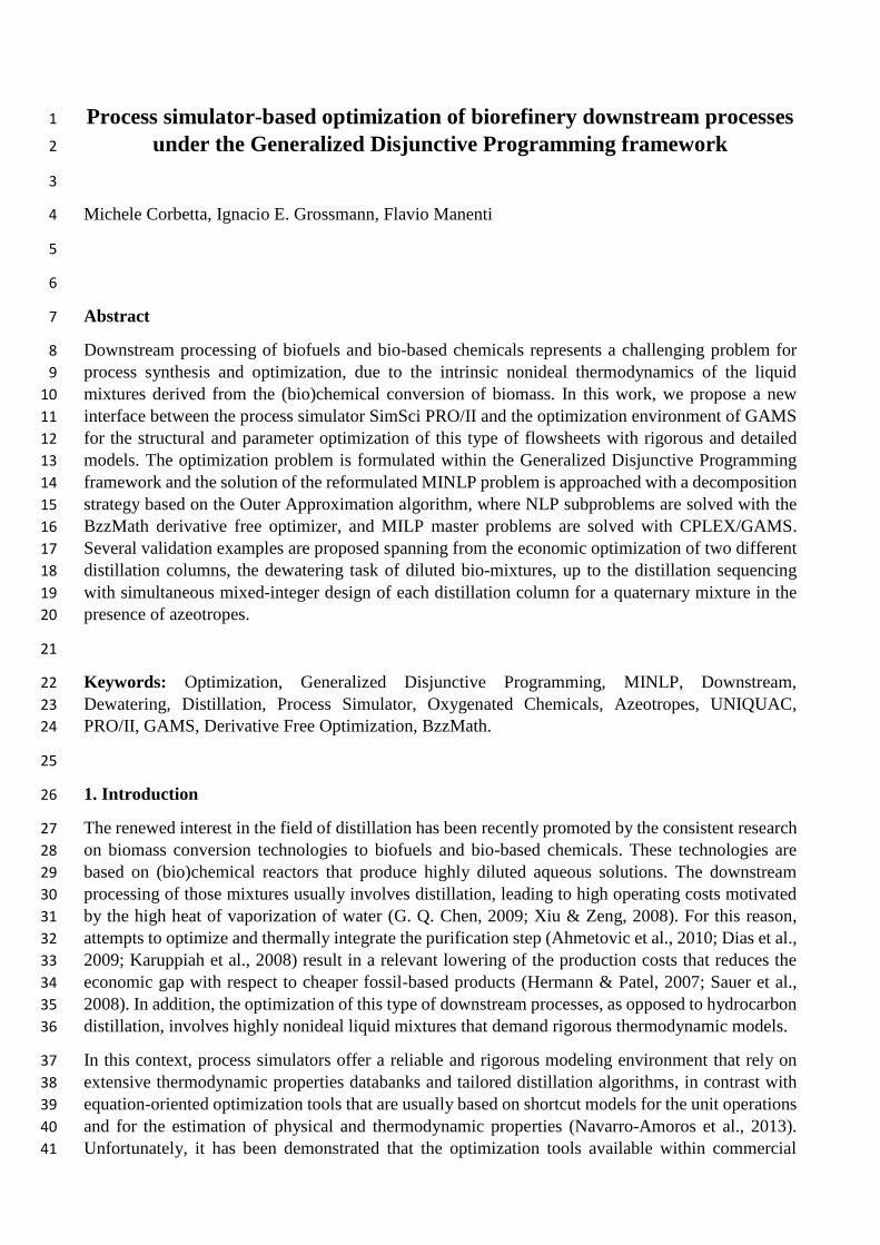
A relevant case of this kind of superstructure arise from the solution of distillation sequencing 40
problems. At this level, it is possible to represent the sequencing with either a State Task Network 41
(STN) or a State Equipment Network (SEN) (Yeomans & Grossmann, 1999). Figure 2 reports the 42

5
two different superstructures for the distillation of a ternary mixture. It is possible to highlight that 1
the SEN requires a smaller number of columns but it introduces recycles. Nevertheless, since the 2
modeling is accomplished by the process simulator with a logic-based definition of the input file that 3
considers only selected units, it does not matter if either STN or SEN superstructure is adopted. 4
5
Figure 1: Representations of the conditional unit&trays elementary module and of a typical 6
superstructure. 7
(a) (b)
Figure 2: (a) State Task Network and (b) State Equipment Network representations for the sharp 8
distillation of a ternary mixture. 9
10
4. Modeling 11
The detailed modeling is achieved with a process simulator (SimSci PRO/II) taking advantage of 12
thermodynamic databanks for the estimation of physical properties and ad-hoc algorithms for the 13
solution of nonlinear systems derived from distillation columns and other unit operations. Within this 14
process modeling environment there is also the flexibility to introduce custom modeling components, 15
which can be required in case of nonconventional unit operations, as discussed elsewhere (Corbetta 16
et al., 2014). 17
4.1 Thermodynamic modeling 18
CONDITIONAL UNIT&TRAYS MODULE
SUPERSTRUCTURE
Fixe
d
Tray
s
CONDITIONAL STRIPPING
TRAYS
CONDITIONAL RECTIFICATION
TRAYS
CONDITIONAL UNIT
LOGIC DEFINED
IF ELSE
A
B
C
A
–
B
C
A
B
–
C
B
–
C
A
–
B
A
B
CB
C
A
B
A
B
C
A
–
B
C
or
A
–
B
A
B
–
C
or
B
–
C
A
B
C
A
B
B
C

6
When the target is to address the synthesis of biorefinery downstream processes, it is worth 1
mentioning that predictive thermodynamic models, such as UNIFAC, frequently fail. This is due to 2
the highly complex nature of the interactions between oxygenated chemicals in the aqueous phase. 3
These complex liquid mixtures can be obtained, for instance, in the form of fermentation broth 4
withdrawn from a bioreactor or from the outlet of catalytic deoxygenation converters, and they 5
present some common characteristics. Usually they are diluted organic aqueous solutions, in which 6
water can represent up to 80-90 wt.%. Moreover, they are made up of a large amount of components 7
that belong to the same chemical class (e.g. ketones, alcohols, polyols), with a frequent occurrence 8
of homogeneous azeotropes and pinch points in the corresponding VLE equilibrium diagrams. 9
Finally, a heavy cut composed by soluble solids is usually present due to incomplete biomass 10
conversion, presence of an inert lignin fraction, and/or production of high molecular weight 11
components by side reactions. Consequently, developing reliable VL(L)E thermodynamic models 12
based on nonlinear regression of (UNIQUAC or NRTL) binary interaction parameters on 13
experimental data (Pirola et al., 2014) plays a major role in correctly predicting the distillation 14
behavior, as will be highlighted in Section 7. 15
4.2 Cost functions 16
Once the process simulator is set up with a proper thermodynamic model, the convergence of a 17
flowsheet provides the value of the implicit variables for the evaluation of the economic objective 18
function and for measuring the violation of nonlinear constraints. Specifically, the techno-economic 19
assessment is approached with nonlinear cost functions (Douglas, 1988) and rigorous sizing models 20
embedded within the process simulator (e.g. tray and packing hydraulics). For distillation columns, 21
the minimization of the cost objective function is performed by considering both annualized capital 22
costs (CAPEX) and operating cost (OPEX), which added together determine the Total Annualized 23
Costs (TAC) as reported in Eq.(1). 24
inv col internals reb condop steam cw entrainer
C C C C CTAC C C C C
payback time payback time
(1) 25
Operating costs include utility costs (steam, cooling water and eventually entrainers), while column 26
investment costs include trays or packing, column vessel, condenser and reboiler installation and 27 purchase costs, which depend on the value of the decision optimization variables and on the size of 28 the equipment. For CAPEX evaluation, the following function, Eq.(2), is adopted, where constants 29
c1, c2, e1 and e2 depend on the equipment type, L1 and L2 are relevant size, Fc is a parameter depending 30 on the fabrication material and operating pressure, while M&S is the Marshall & Swift economic 31
index. 32
1 2
1 1 2 2 ,
&[$] ( F )
280
e e
equipment C equiment
M SC c L L c
(2) 33
4.3 Generalized Disjunctive Programming formulation 34
The optimization problem is formulated within the Generalized Disjunctive Programming framework 35
(Grossmann & Trespalacios, 2013), in which also implicit variables (xI) are assumed, along with 36
continuous decision variables (x) and Boolean decision variables (Y), as outlined in Eq.(3). These 37
implicit variables are evaluated by the process simulator, which is treated as a black-box and is 38
represented by the implicit function (fI) that links implicit variables with decision variables. Nonlinear 39
constraints (g) can be both global (set G) and conditional (set Gk). The mathematical programming 40
formulation involves the definition of a set K of disjunctions, corresponding to conditional unit&trays 41
7
modules, for which additional constraints, equations, and cost contributions are defined. Each 1
disjunction involves only two terms, corresponding to the selection or not of a conditional unit ( kY ), 2
with embedded disjunctions for the conditional trays (jY ) belonging to each elementary module (set 3
of CTk conditional rectification and stripping trays of column k). The economic objective function 4
includes these contributions along with a general function ( ,fI
x x ) of the decision variables. 5
Finally, the propositional logic defines the units’ interconnectivity. Topology logic (6
topology kY true ) defines the interconnection between conditional units, while the three subsequent 7
sets of logic constraints are required to ensure that no conditional trays are selected if the conditional 8
unit is not selected, at most only one Boolean variable should be true for the rectification (RCTk) and 9
for the stripping (SCTk) conditional trays of each distillation column (either permanent or 10
conditional). 11
,
I
min ,
s.t. ' ''
' '
, 0
0
''
, 0
(x, y, x )k
k
k K
I
n
k
j j
j j j
I k I
n
k j
j CT
Z TAC f
f
g n G
Y
Y Y
TAC TAC
x '' f
g
TAC
I
I I I
I
I
I
x x
x x x
x x
x x
x
x x
,
k
0 , ,
0
,
,
k
I k k k
k
topology k
j k
i k
i
Y
x '' j CT n G k K
TAC
Y true
Y Y k K j CT
Y i RCT k K
Y
,
, , , ;I
k
mnn m
i SCT k K
true false
L U
I
x x x
x x c Y
(3) 12
13
5. Optimization algorithm 14
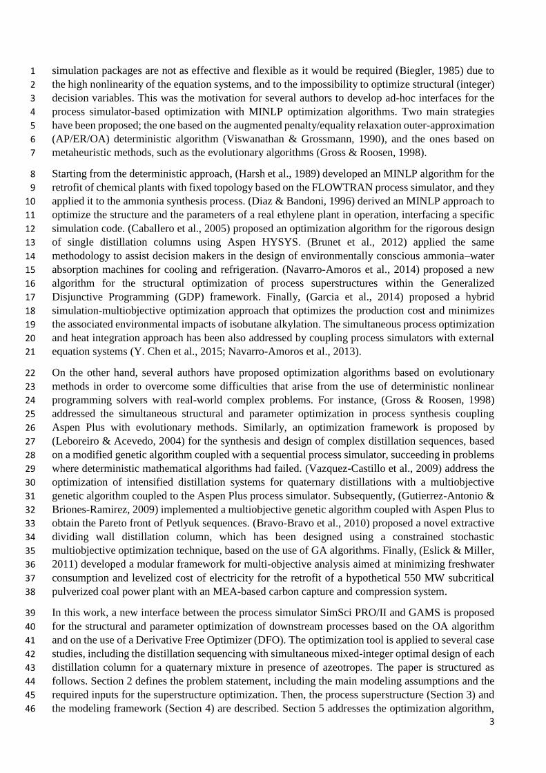
The optimization problem is solved with a decomposition strategy based on the Logic-Based Outer 15
Approximation (LBOA) algorithm (Turkay & Grossmann, 1996). The algorithm involves NLP 16
subproblems that arise from fixed values at the Boolean variables Y in Eq.(3), and MILP master 17
problems that correspond to a linear approximation at the GDP in Eq.(3). NLP subproblems are solved 18
with a Derivative Free Optimizer (C++/BzzMath), and MILP master problems are solved with Branch 19
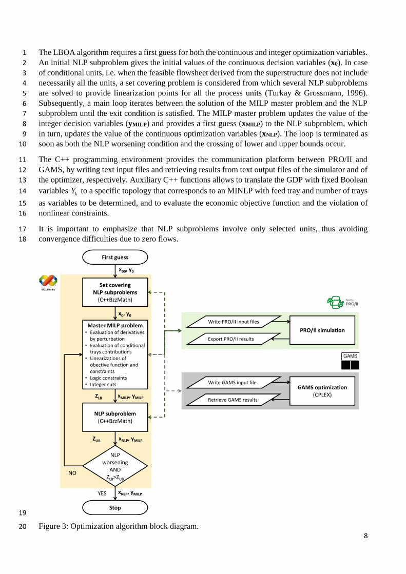
& Cut methods (GAMS/CPLEX). The corresponding block diagram of this algorithm is shown in 20
Figure 3. 21
8
The LBOA algorithm requires a first guess for both the continuous and integer optimization variables. 1
An initial NLP subproblem gives the initial values of the continuous decision variables (x0). In case 2
of conditional units, i.e. when the feasible flowsheet derived from the superstructure does not include 3
necessarily all the units, a set covering problem is considered from which several NLP subproblems 4
are solved to provide linearization points for all the process units (Turkay & Grossmann, 1996). 5
Subsequently, a main loop iterates between the solution of the MILP master problem and the NLP 6
subproblem until the exit condition is satisfied. The MILP master problem updates the value of the 7
integer decision variables (yMILP) and provides a first guess (xMILP) to the NLP subproblem, which 8
in turn, updates the value of the continuous optimization variables (xNLP). The loop is terminated as 9
soon as both the NLP worsening condition and the crossing of lower and upper bounds occur. 10
The C++ programming environment provides the communication platform between PRO/II and 11
GAMS, by writing text input files and retrieving results from text output files of the simulator and of 12
the optimizer, respectively. Auxiliary C++ functions allows to translate the GDP with fixed Boolean 13
variables kY to a specific topology that corresponds to an MINLP with feed tray and number of trays 14
as variables to be determined, and to evaluate the economic objective function and the violation of 15
nonlinear constraints. 16
It is important to emphasize that NLP subproblems involve only selected units, thus avoiding 17
convergence difficulties due to zero flows. 18
19
Figure 3: Optimization algorithm block diagram. 20
Set coveringNLP subproblems
(C++BzzMath)
First guess
NLP worsening
AND ZLB>ZUB
Write PRO/II input files
x00, y0
x0, y0
Master MILP problem• Evaluation of derivatives
by perturbation• Evaluation of conditional
trays contributions• Linearizations of
obective function and constraints
• Logic constraints• Integer cuts
PRO/II simulation
Export PRO/II results
Write GAMS input fileGAMS optimization
(CPLEX)Retrieve GAMS results
NLP subproblem(C++BzzMath)
Stop
xMILP, yMILP
xNLP, yMILPZUB
ZLB
xNLP, yMILPYES
NO
9
5.1 NLP subproblem 1
NLP subproblems are solved with the Derivative Free Optimizer belonging to the BzzMath numerical 2
library (Buzzi-Ferraris & Manenti, 2012), which is available online at http://super.chem.polimi.it/. 3
The BzzMinimizationRobust is based on a modified Nelder-Mead Simplex direct search 4
method (OPTNOV variant), which has proved to handle problems with highly nonlinear, 5
nondifferentiable and discontinuos functions, and problems with narrow valleys (Buzzi-Ferraris, 6
1967; G. Buzzi-Ferraris & F. Manenti, 2010). 7
Nonlinear constraints of the NLP subproblems (in the form , 0g I
x x ) are handled with a penalty 8
function proportional to the constraint violation that is added to the objective function, allowing to 9
start with an infeasible first guess. A Sequential Unconstrained Minimization Technique (Correia et 10
al., 2010) is adopted by progressively increasing the penalty weight (mgw ) in order to limit difficulties 11
with narrow valleys. 12
The n-th subproblem, corresponding to the yn integer variables, is reported in Eq.(4), where the first 13
set of constraints derives from the convex-hull reformulation of the disjunctions (Grossmann & 14
Trespalacios, 2013). These constraints force the decision variables of the non-selected units ( 0ky 15
) to be zero. 16
min , max 0; ( , )
s.t.
i
k
UB
n n k n g i
k K i G G
L U
k k k k k
n
Z TAC f w g
y x x y x k K
I Ix
y y x x x x
x
(4) 17
5.2 MILP master problem 18
The MILP master problem, reported in Eq.(5), is a linearization of the original nonlinear problem, 19
which includes accumulated linearizations of the objective function and of the constraints, logic 20
constraints representing the interconnectivity among process units within the superstructure, integer 21
cuts, and convex-hull constraints derived from the reformulation of the disjunctions. 22
,
min
. . ( , , ) ( , , )(x x )
( , , ) ( , , )(x x ) i
LB l l
OA f g
l L
objl l l l l l l l
obj i i i i f
i iX t CTi
l l l l l l l lnn i i t t g
i iX t CTi
Z w slack slack
fs t f y slack l L
x
gg y slack
x
x y
I I
I I
x y x x y x
x y x x y x ,
y ( , , ) ( , , )(x x ) , ,
y y 1
,
i
l l l l l l l lnk n i i t t g k
i iX t CTi
i i
i B i N
L U
k k k k k
n
n G l L
gg y slack n G k K l L
x
B
y x x y x k K
I I
L U
x y x x y x
Ay b
x x x
x 0;1 , , , m l l
f gslack slack l L y
(5) 23
10
Accumulated linearizations are obtained using as linearization points ( , ,l l l
Ix y x ) those that are 1
obtained from all the previous NLP subproblems, derivatives with respect to the continuous decision 2
variables, and delta contributions ( i , i ) associated to each conditional tray. It should be noted that 3
the set L defines all the previous main iterations, including the ones of the set covering problem. 4
Moreover, slack variables are added to the linearization cuts to handle feasible region and objective 5
function nonconvexities. They allow to find possible better solutions in the surrounding of the 6
linearized nonconvex feasible region (Viswanathan & Grossmann, 1990). It should be noted that the 7
integer constraints in the form Ay b , are the translation of the propositional logic in Eq.(3) that 8
defines the superstructure topology in the GDP representation (Grossmann & Trespalacios, 2013). 9
Derivatives of objective function and constraints are found to be very important for the effectiveness 10
of the master problem. In fact, an inaccurate linearization of the objective function can cut-off optimal 11
solutions, while inaccurate linearizations of constraints can cut-off feasible region areas (potentially 12
excluding the optimal solution). Using a process simulator does not allow one to directly access 13
analytical derivatives. For this reason, the finite difference based on perturbations has been adopted. 14
From an analytical point of view, perturbations should be as small as possible to ensure good 15
derivative estimates. However, it is crucial to mention that decreasing the value of the perturbation 16
results in increasing the error due to the noise of the NLP solvers embedded within process simulators. 17
As a result, there is a trade-off between accuracy and noise for small values of the perturbation, and 18
depending on the decision variable and on the linearization point, there is an optimal range of 19
perturbation. For this reason, a perturbation test is performed for each continuous decision variable 20
at each MILP main iteration. The derivative is estimated starting from a larger perturbation; then the 21
perturbation is halved and this procedure is iterated until the relative change of the derivative is below 22
a certain tolerance. Typical values of the perturbations are in the range of 10-3 to 10-4. 23
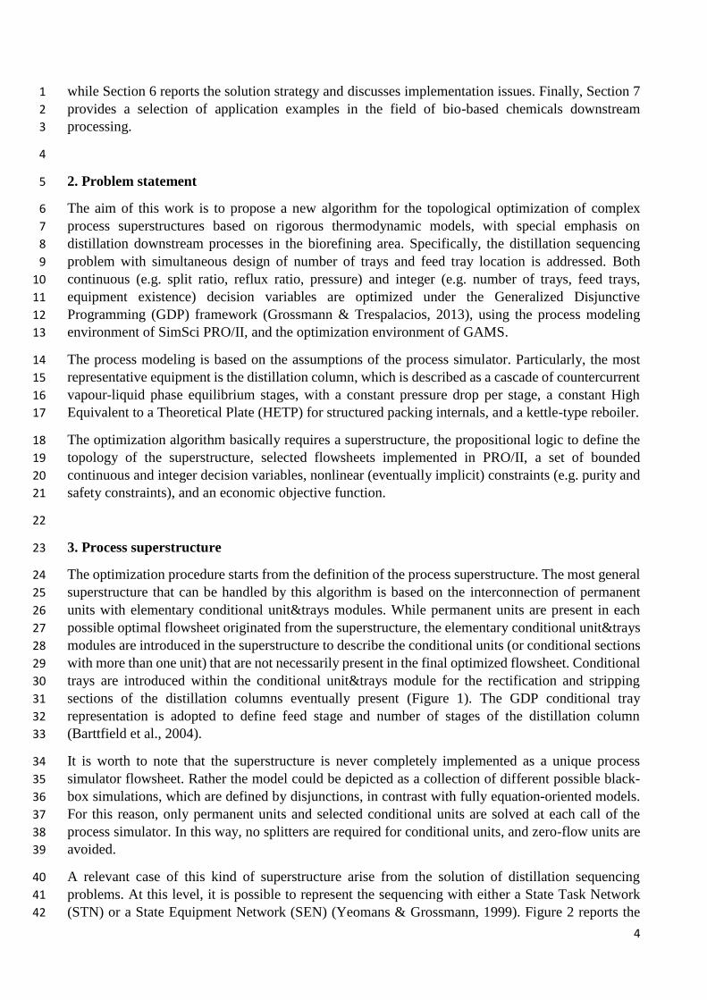
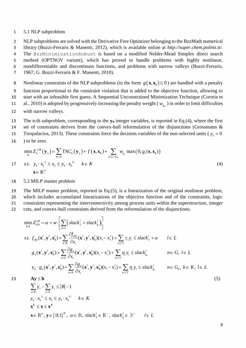
Delta contributions of a conditional tray for the objective function ( i ) and for nonlinear constraints 24
( i ) are computed by converging a flowsheet that differs from the i-th linearization point only for the 25
number of trays of the distillation section to which the conditional tray belongs, as outlined in Figure 26
4. 27
28
Figure 4: Procedure to evaluate delta contributions of rectification and stripping conditional trays 29
(Caballero et al., 2005). 30
i-th iteration
Rectification Conditional Trays (RCT) i-th delta contributions
Stripping Conditional Trays (SCT) i-th delta contributions
yRCTNyRCT2yRCT1
ySCTNySCT2ySCT1

11
6. Solution strategy and remarks 1
The success of this optimization algorithm is strongly influenced by a careful formulation of the 2
problem and by the selection of proper parameters and settings. 3
The problem should be formulated selecting continuous and discrete decision variables that lead to a 4
fast and easy convergence of the process simulator flowsheet with all the values in the range between 5
lower and upper bounds. This is true especially for distillation columns, for which two specifications 6
should be provided, along with the number of trays and feed tray. The two continuous decision 7
variables are usually imposed as reflux ratio and bottom to feed ratio, or, in case of distillation 8
sequencing, they can be the light key component recovery at the overhead and the heavy key 9
component recovery at the bottom. It is sometimes useful to insert a few fixed trays in the rectification 10
and in the stripping sections. This means that the permanent stages are not only the feed tray, the 11
condenser and the reboiler, but also a suitable small number of trays above and below the feed, based 12
on the separation requirements that can be checked at the end of the optimization procedure. This 13
strategy helps the convergence of the column and avoids the solution of columns with a number of 14
trays that is too small (such as only 3 trays), thus reducing the number of evaluation for the conditional 15
trays delta contributions and speeding up the solution of the MILP master problem. 16
On the other hand, there are two main sets of parameters to consider: the ones related to the 17
optimization algorithm, and the ones related to the SimSci PRO/II process simulator settings. 18
Optimization parameters include perturbation step size and penalty weights for the NLP and MILP 19
problems. Perturbation step size is selected based on the aforementioned adaptive step size strategy. 20
Penalty weights for the violation of nonlinear constraints can be selected with the same order of 21
magnitude of the objective function and can be successively increased with a SUMT procedure 22
(Correia et al., 2010), while penalty weights for slack variables are found not to have a significant 23
impact on the solution of the optimization problem. SimSci PRO/II simulation settings, in turn, should 24
be carefully tuned, depending on the distillation column that is to be solved. At first, a suitable 25
distillation algorithm should be selected. In this work, the CHEMDIST algorithm (Bondy, 1991) has 26
been selected for the VLLE heteroextractive distillation column case study, while the INPUT-27
OUTPUT algorithm (Russell, 1983) for the other conventional columns. To ensure the convergence 28
of the columns, three key settings are mandatory, i.e. initial estimates model, damping factor, and 29
homotopy. The initialization model provides temperature estimates and either vapor or liquid molar 30
flow rate estimates to initiate the iterative calculations. The selection of a suitable method equally 31
depends on the distillation system. The CHEMICAL initialization model is adopted for complex 32
thermodynamic systems and it is based on a multi-flash technique to bring the profiles closer to the 33
final solution before the column algorithm takes over. Another option is to use the CONVENTIONAL 34
initialization model that it is based on the Fenske shortcut model; it is less CPU intensive and it is 35
recommended when nonidealities are less strong. On the other side, the damping factor should be 36
reduced from 1 to a value below 0.5 for oscillating systems, while homotopy could be adopted if the 37
previous strategies fail. 38
Typical problem size should not exceed 10 continuous decision variables in the NLP subproblems, 39
due to the intrinsic limit of DFO solvers (Rios & Sahinidis, 2013), but can reach several hundreds of 40
discrete decision variables in the MILP master problems. The overall number of continuous decision 41
variables in the MILP could be much greater than 10, because in the NLP subproblems only selected 42
conditional units are accounted for, along with their decision variables. The ratio between computing 43
times for the NLP and MILP problems is proportional to the ratio between continuous and discrete 44

12
decision variables, and the MILP computing time is largely due to the evaluation of conditional trays 1
delta contributions for objective function and constraints. 2
3
7. Application examples 4
The optimization algorithm is applied to four different case studies, dealing with the purification of 5
aqueous solutions of oxygenated chemicals derived from biorefining. These flowsheets essentially 6
include distillation columns with a highly nonideal liquid phase, considered with the UNIQUAC 7
liquid activity coefficient model. The first case study introduces this methodology to a single 8
distillation column with one homogeneous azeotropes; the second case study involves a two-liquid 9
phase heteroextractive distillation column with an heterogeneous azeotrope; the third case study 10
includes the dewatering section of a downstream process with thermally coupled multieffect 11
distillation columns; finally, the last example addresses the distillation sequencing of a bio-mixture. 12
For each application example, scope, thermodynamic modeling, problem formulation and results are 13
provided, along with remarks and comments. The significant importance of developing reliable 14
VL(L)E thermodynamic models based on nonlinear regression on experimental data is highlighted in 15
the following section. 16
7.1 Single distillation column 17
The first case study takes in consideration a single multicomponent distillation column that realizes 18
the cut between 1,2-propylene glycol (1,2-PG) and ethylene glycol (EG), which are mixed with other 19
co-products obtained from the hydroprocessing of lignocellulosic sugars. The feed is composed by 20
40 wt.% EG, 50 wt.% 1,2-PG and 10 wt.% of mixed heavier oxygenated chemicals that form also an 21
homogeneous azeotrope with EG. The distillation column with structured packing internals is 22
operated at atmospheric pressure with a total condenser and a kettle reboiler. The aim of the 23
optimization is to determine the optimal number of trays, feed tray location, and the value of the two 24
specifications (reflux ratio and bottom flowrate) that minimize TAC, with purity constraints at the 25
top and at the bottom for 1,2-PG and EG, respectively. 26
The first step for an effective optimization of bio-mixtures is the definition of a reliable 27
thermodynamic model. Binary interaction parameters and predictive models included in process 28
simulators for this kind of components are most of the times not reliable. For this reason, UNIQUAC 29
binary interaction parameters have been estimated by nonlinear regression with the 30
BzzNonlinearRegression class of the BzzMath library (Buzzi-Ferraris & Manenti, 2009; G. 31
Buzzi-Ferraris & F. Manenti, 2010; Pirola et al., 2014), using published phase equilibrium 32
experimental data (Yang et al., 2014; Zhang et al., 2013; Zhong et al., 2014). Only two representative 33
VLE Txy plots are reported in Figure 5 for the sake of conciseness. 34
The first guess for the decision variables has been derived by preliminary short-cut evaluations and 35
involves a column with 123 stages (HETP = 0.250 m) with the feed at the 92nd stage. The evolution 36
of the objective function over the main iterations is reported for both the MILP lower bound and the 37
NLP upper bound in Figure 6a. The optimal configuration is found at the third iteration (red dashed 38
line), with 135 stages and the feed at the 98th stage, because there is the simultaneous crossing between 39
lower and upper bounds and the worsening of the NLP. Table 1 summarizes the most important 40
indicators of the case study 1. It is worth noting that the number of discrete decision variables (40) 41
derives from the number of conditional trays, 20 for the rectification and 20 for the stripping sections. 42

13
1
Figure 5: Txy VLE plots of 1,2-PG and EG with 2,3-butanediol at 1 bar. Experimental data (symbols) 2
and model predictions (lines). 3
(a) (b)
(c) (d)
Figure 6: Evolution of objective function (a), structural decision variables (b) and continuous decision 4
variables (c-d) of case study 1 as a function of the OA main iterations. The dashed line reports the 5
first guess given by the MILP master problem. 6
452
453
454
455
456
457
458
459
460
461
0 0.2 0.4 0.6 0.8 1
Tem
per
atu
re [
K]
x1, y1
Tb (Zhong et al., 2014)
Td (Zhong et al., 2014)
Tb WILSON BzzMath
Td WILSON BzzMath
Tb UNIQUAC BzzMath
Td UNIQUAC BzzMath
VLE (1) PG/ (2) 2,3-BDO @ 1 bar452
454
456
458
460
462
464
466
468
470
472
0 0.2 0.4 0.6 0.8 1
Tem
per
atu
re [
K]
x1, y1
VLE (1) EG/ (2) 2,3-BDO @ 1 bar
Tb (Zhong et al., 2014)
Td (Zhong et al., 2014)
Td UNIQUAC BzzMath
Tb UNIQUAC BzzMath
Tb WILSON BzzMath
Td WILSON BzzMath
1.800E+06
1.805E+06
1.810E+06
1.815E+06
1.820E+06
0 1 2 3 4
Main iterations
TAC [$/y]
NLP Subproblem
MILP Master problem
0
20
40
60
80
100
120
140
0 1 2 3 4
Main iterations
Column topology
FeedTray
Ntrays
43.5
43.6
43.7
43.8
43.9
44
0 1 2 3 4
Main iterations
Bottom flowrate [kmol/h]
4.5
4.7
4.9
5.1
5.3
5.5
0 1 2 3 4
Main iterations
Reflux ratio
14
Table 1: Summary of case study 1. 1
Number of continuous decision variables 2
Number of discrete decision variables 40
Number of nonlinear constraints 2
Objective function of the first guess 3,986,700 $/y
Objective function of the optimal solution 1,803,370 $/y
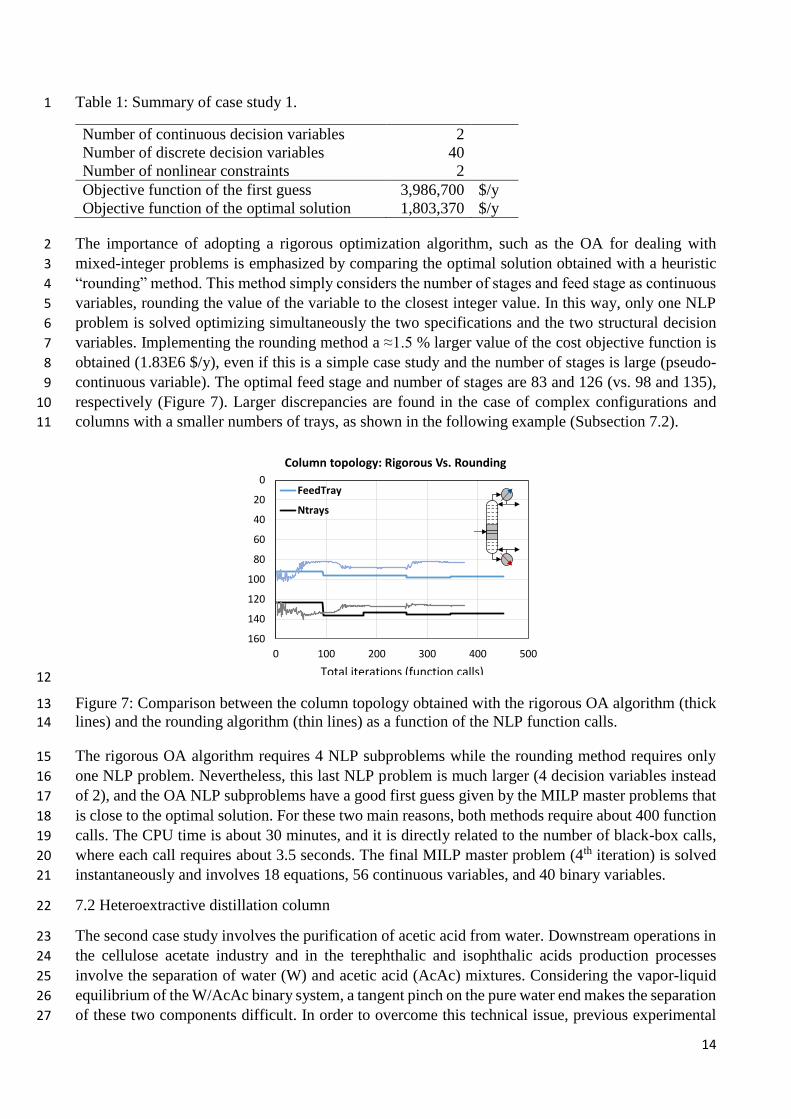
The importance of adopting a rigorous optimization algorithm, such as the OA for dealing with 2
mixed-integer problems is emphasized by comparing the optimal solution obtained with a heuristic 3
“rounding” method. This method simply considers the number of stages and feed stage as continuous 4
variables, rounding the value of the variable to the closest integer value. In this way, only one NLP 5
problem is solved optimizing simultaneously the two specifications and the two structural decision 6
variables. Implementing the rounding method a ≈1.5 % larger value of the cost objective function is 7
obtained (1.83E6 $/y), even if this is a simple case study and the number of stages is large (pseudo- 8
continuous variable). The optimal feed stage and number of stages are 83 and 126 (vs. 98 and 135), 9
respectively (Figure 7). Larger discrepancies are found in the case of complex configurations and 10
columns with a smaller numbers of trays, as shown in the following example (Subsection 7.2). 11
12
Figure 7: Comparison between the column topology obtained with the rigorous OA algorithm (thick 13
lines) and the rounding algorithm (thin lines) as a function of the NLP function calls. 14
The rigorous OA algorithm requires 4 NLP subproblems while the rounding method requires only 15
one NLP problem. Nevertheless, this last NLP problem is much larger (4 decision variables instead 16
of 2), and the OA NLP subproblems have a good first guess given by the MILP master problems that 17
is close to the optimal solution. For these two main reasons, both methods require about 400 function 18
calls. The CPU time is about 30 minutes, and it is directly related to the number of black-box calls, 19
where each call requires about 3.5 seconds. The final MILP master problem (4th iteration) is solved 20
instantaneously and involves 18 equations, 56 continuous variables, and 40 binary variables. 21
7.2 Heteroextractive distillation column 22
The second case study involves the purification of acetic acid from water. Downstream operations in 23
the cellulose acetate industry and in the terephthalic and isophthalic acids production processes 24
involve the separation of water (W) and acetic acid (AcAc) mixtures. Considering the vapor-liquid 25
equilibrium of the W/AcAc binary system, a tangent pinch on the pure water end makes the separation 26
of these two components difficult. In order to overcome this technical issue, previous experimental 27
0
20
40
60
80
100
120
140
160
0 100 200 300 400 500
Column topology: Rigorous Vs. Rounding
FeedTray
Ntrays
Total iterations (function calls)
15
and modeling studies (Pirola et al., 2014) showed that p-xylene (pX) is a suitable entrainer to operate 1
a heterogeneous extractive distillation. The miscibility gap between W and pX is exploited to separate 2
the distillate stream in a decanter where an aqueous and an organic phase are obtained. The organic 3
phase is composed of nearly pure pX that is recycled back as entrainer to the top section of the column, 4
while the aqueous stream with traces of AcAc is withdrawn and sent to wastewater treatment. From 5
the bottom of the heteroextractive column, a stream composed by AcAc, and the excess of the 6
extractive entrainer is recycled back to the upstream synthesis process. 7
Reliable thermodynamic models, based on the UNIQUAC liquid activity model, have been developed 8
elsewhere (Pirola et al., 2014), and are hereinafter adopted to perform the economic optimization of 9
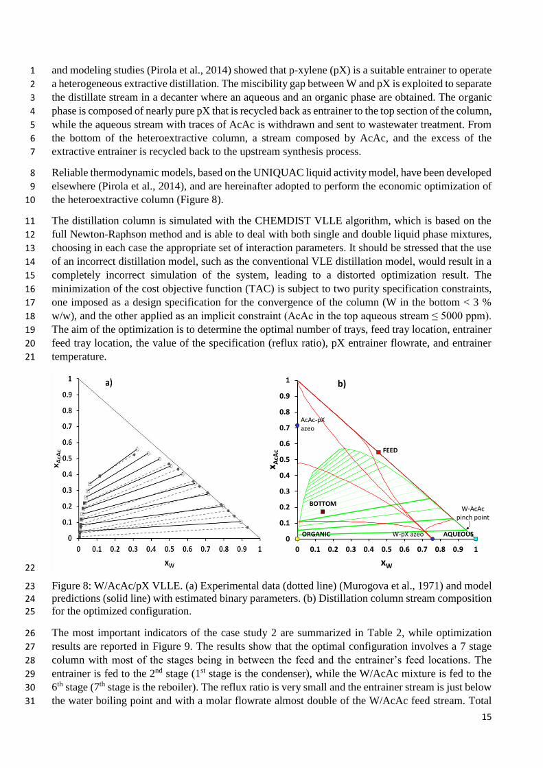
the heteroextractive column (Figure 8). 10
The distillation column is simulated with the CHEMDIST VLLE algorithm, which is based on the 11
full Newton-Raphson method and is able to deal with both single and double liquid phase mixtures, 12
choosing in each case the appropriate set of interaction parameters. It should be stressed that the use 13
of an incorrect distillation model, such as the conventional VLE distillation model, would result in a 14
completely incorrect simulation of the system, leading to a distorted optimization result. The 15
minimization of the cost objective function (TAC) is subject to two purity specification constraints, 16
one imposed as a design specification for the convergence of the column (W in the bottom < 3 % 17
w/w), and the other applied as an implicit constraint (AcAc in the top aqueous stream ≤ 5000 ppm). 18
The aim of the optimization is to determine the optimal number of trays, feed tray location, entrainer 19
feed tray location, the value of the specification (reflux ratio), pX entrainer flowrate, and entrainer 20
temperature. 21
22
Figure 8: W/AcAc/pX VLLE. (a) Experimental data (dotted line) (Murogova et al., 1971) and model 23
predictions (solid line) with estimated binary parameters. (b) Distillation column stream composition 24
for the optimized configuration. 25
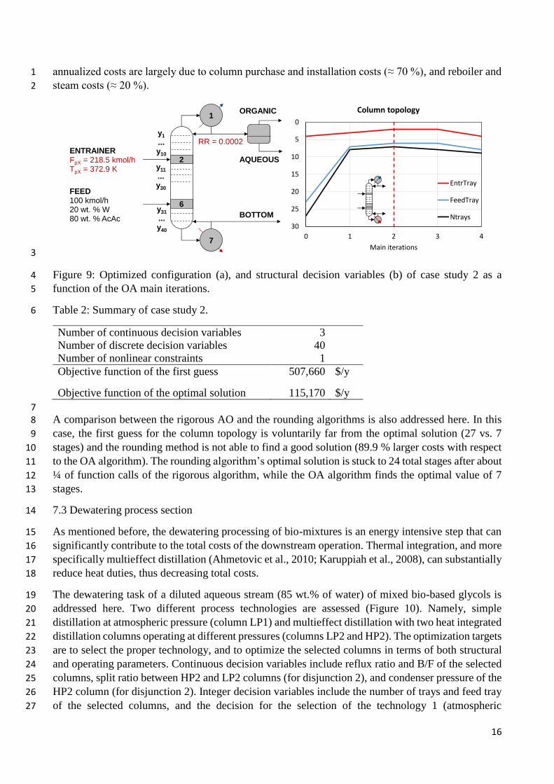
The most important indicators of the case study 2 are summarized in Table 2, while optimization 26
results are reported in Figure 9. The results show that the optimal configuration involves a 7 stage 27
column with most of the stages being in between the feed and the entrainer’s feed locations. The 28
entrainer is fed to the 2nd stage (1st stage is the condenser), while the W/AcAc mixture is fed to the 29
6th stage (7th stage is the reboiler). The reflux ratio is very small and the entrainer stream is just below 30
the water boiling point and with a molar flowrate almost double of the W/AcAc feed stream. Total 31
0
0.1
0.2
0.3
0.4
0.5
0.6
0.7
0.8
0.9
1
0 0.1 0.2 0.3 0.4 0.5 0.6 0.7 0.8 0.9 1
x AcA
c
xW
FEED
BOTTOM
AQUEOUSORGANIC
AcAc-pXazeo
W-pX azeo
W-AcAcpinch point
b)
16
annualized costs are largely due to column purchase and installation costs (≈ 70 %), and reboiler and 1
steam costs (≈ 20 %). 2
3
Figure 9: Optimized configuration (a), and structural decision variables (b) of case study 2 as a 4
function of the OA main iterations. 5
Table 2: Summary of case study 2. 6
Number of continuous decision variables 3
Number of discrete decision variables 40
Number of nonlinear constraints 1
Objective function of the first guess 507,660 $/y
Objective function of the optimal solution 115,170 $/y
7 A comparison between the rigorous AO and the rounding algorithms is also addressed here. In this 8
case, the first guess for the column topology is voluntarily far from the optimal solution (27 vs. 7 9
stages) and the rounding method is not able to find a good solution (89.9 % larger costs with respect 10
to the OA algorithm). The rounding algorithm’s optimal solution is stuck to 24 total stages after about 11
¼ of function calls of the rigorous algorithm, while the OA algorithm finds the optimal value of 7 12
stages. 13
7.3 Dewatering process section 14
As mentioned before, the dewatering processing of bio-mixtures is an energy intensive step that can 15
significantly contribute to the total costs of the downstream operation. Thermal integration, and more 16
specifically multieffect distillation (Ahmetovic et al., 2010; Karuppiah et al., 2008), can substantially 17
reduce heat duties, thus decreasing total costs. 18
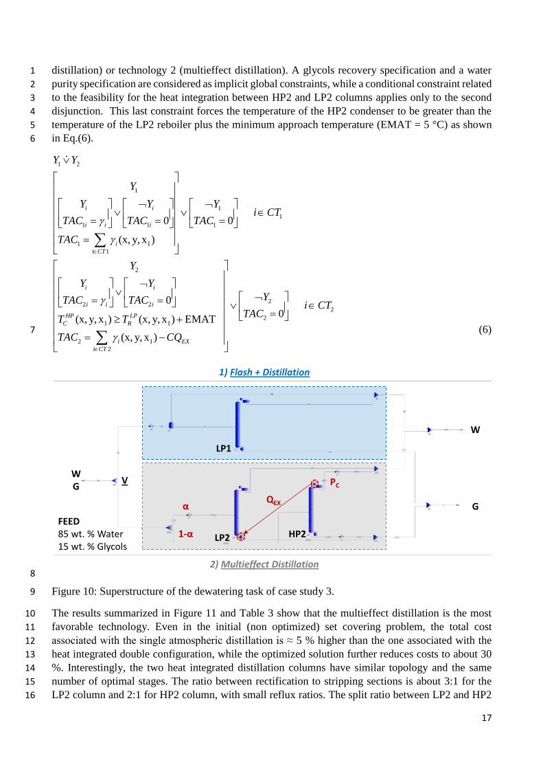
The dewatering task of a diluted aqueous stream (85 wt.% of water) of mixed bio-based glycols is 19
addressed here. Two different process technologies are assessed (Figure 10). Namely, simple 20
distillation at atmospheric pressure (column LP1) and multieffect distillation with two heat integrated 21
distillation columns operating at different pressures (columns LP2 and HP2). The optimization targets 22
are to select the proper technology, and to optimize the selected columns in terms of both structural 23
and operating parameters. Continuous decision variables include reflux ratio and B/F of the selected 24
columns, split ratio between HP2 and LP2 columns (for disjunction 2), and condenser pressure of the 25
HP2 column (for disjunction 2). Integer decision variables include the number of trays and feed tray 26
of the selected columns, and the decision for the selection of the technology 1 (atmospheric 27
1
7
6
RR = 0.0002
FEED 100 kmol/h20 wt. % W80 wt. % AcAc
y1
...y10
y31
...y40
2ENTRAINERFpX = 218.5 kmol/hTpX = 372.9 K y11
...y30
BOTTOM
ORGANIC
AQUEOUS
0
5
10
15
20
25
30
0 1 2 3 4
Main iterations
Column topology
EntrTray
FeedTray
Ntrays
17
distillation) or technology 2 (multieffect distillation). A glycols recovery specification and a water 1
purity specification are considered as implicit global constraints, while a conditional constraint related 2
to the feasibility for the heat integration between HP2 and LP2 columns applies only to the second 3
disjunction. This last constraint forces the temperature of the HP2 condenser to be greater than the 4
temperature of the LP2 reboiler plus the minimum approach temperature (EMAT = 5 °C) as shown 5
in Eq.(6). 6
1 2
1
1
1
1 1 1
1 I
1
2
2
0 0
(x, y, x )
i i
i i i
i
i CT
i
i i
Y Y
Y
Y Y Yi CT
TAC TAC TAC
TAC
Y
Y
TAC
22
2
2I I
2 I
2
0
0(x, y, x ) (x, y, x ) EMAT
(x, y, x )
i
i
HP LP
C R
i EX
i CT
Y
YTACi CT
TACT T
TAC CQ
(6) 7
8
Figure 10: Superstructure of the dewatering task of case study 3. 9
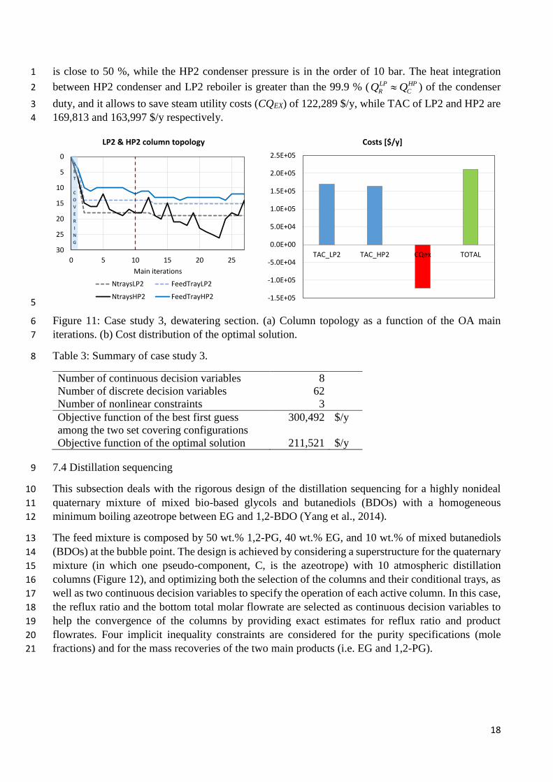
The results summarized in Figure 11 and Table 3 show that the multieffect distillation is the most 10
favorable technology. Even in the initial (non optimized) set covering problem, the total cost 11
associated with the single atmospheric distillation is ≈ 5 % higher than the one associated with the 12
heat integrated double configuration, while the optimized solution further reduces costs to about 30 13
%. Interestingly, the two heat integrated distillation columns have similar topology and the same 14
number of optimal stages. The ratio between rectification to stripping sections is about 3:1 for the 15
LP2 column and 2:1 for HP2 column, with small reflux ratios. The split ratio between LP2 and HP2 16
2) Multieffect Distillation
1) Flash + Distillation
V
G
W
WG
LP1
HP2LP2
FEED85 wt. % Water15 wt. % Glycols
QEX
PC
α
1-α
18
is close to 50 %, while the HP2 condenser pressure is in the order of 10 bar. The heat integration 1
between HP2 condenser and LP2 reboiler is greater than the 99.9 % ( LP HP
R CQ Q ) of the condenser 2
duty, and it allows to save steam utility costs (CQEX) of 122,289 $/y, while TAC of LP2 and HP2 are 3
169,813 and 163,997 $/y respectively. 4
5
Figure 11: Case study 3, dewatering section. (a) Column topology as a function of the OA main 6
iterations. (b) Cost distribution of the optimal solution. 7
Table 3: Summary of case study 3. 8
Number of continuous decision variables 8
Number of discrete decision variables 62
Number of nonlinear constraints 3
Objective function of the best first guess
among the two set covering configurations
300,492 $/y
Objective function of the optimal solution 211,521 $/y
7.4 Distillation sequencing 9
This subsection deals with the rigorous design of the distillation sequencing for a highly nonideal 10
quaternary mixture of mixed bio-based glycols and butanediols (BDOs) with a homogeneous 11
minimum boiling azeotrope between EG and 1,2-BDO (Yang et al., 2014). 12
The feed mixture is composed by 50 wt.% 1,2-PG, 40 wt.% EG, and 10 wt.% of mixed butanediols 13
(BDOs) at the bubble point. The design is achieved by considering a superstructure for the quaternary 14
mixture (in which one pseudo-component, C, is the azeotrope) with 10 atmospheric distillation 15
columns (Figure 12), and optimizing both the selection of the columns and their conditional trays, as 16
well as two continuous decision variables to specify the operation of each active column. In this case, 17
the reflux ratio and the bottom total molar flowrate are selected as continuous decision variables to 18
help the convergence of the columns by providing exact estimates for reflux ratio and product 19
flowrates. Four implicit inequality constraints are considered for the purity specifications (mole 20
fractions) and for the mass recoveries of the two main products (i.e. EG and 1,2-PG). 21
-1.5E+05
-1.0E+05
-5.0E+04
0.0E+00
5.0E+04
1.0E+05
1.5E+05
2.0E+05
2.5E+05
TAC_LP2 TAC_HP2 CQex TOTAL
Costs [$/y]
0
5
10
15
20
25
30
0 5 10 15 20 25
Main iterations
LP2 & HP2 column topology
NtraysLP2 FeedTrayLP2
NtraysHP2 FeedTrayHP2
S
E
T
C
O
V
E
R
I
N
G

19
1
Figure 12: Superstructure of the distillation sequencing for a quaternary mixture (case study 4). 2
The propositional logic defining the superstructure is reported in Eq.(7) for the sake of completeness, 3
and results in the decision among 5 possible separation process layouts. 4
1 2 3
4 5
6 7
8 9 10
1 4 5
2 8 10
3 6 7
4 10
5 9
6 9
7 8
Y Y Y
Y Y
Y Y
Y Y Y
Y Y Y
Y Y Y
Y Y Y
Y Y
Y Y
Y Y
Y Y
(7) 5
An additional cut, Eq.(8), is added to the constraints of the MILP master problems to enforce the 6
selection of only three distillation column, which is the minimum number required for the separation 7
of four components (NC - 1). 8
A
B
C
D
A
B
–
C
D
A
–
B
C
D
A
B
C
–
D
B
–
C
D
B
C
–
D
A
–
B
C
A
B
–
C
A
–
B
B
–
C
C
–
D
A
B
C
D
1
2
3
4
5
6
7
8
9
10
FEED50 wt. % 12PG40 wt. % EG5 wt. % 12BDO5 wt. % 23BDO

20
3i
i COL
y
(8) 1
The results are summarized in Figure 13 and Table 4. The selected configuration is the sequence of 2
columns 2/8/10 that first realize the central cut between 1,2-PG and EG and then purify the two main 3
products from butanediols (BDOs). Considering the set covering problem, keeping the same total 4
number of trays, the configurations 1/4/10, 1/5/9, 3/6/9, 3/7/8 have 24 %, 96 %, 67 % and 64 % higher 5
extra total annualized costs. The second best configuration is the direct sequence (1/4/10), while the 6
worst configuration is the 1/5/9 that requires higher reflux ratios to avoid violating the purity and 7
recovery constraints. For the optimized columns topology, the cost distribution among the selected 8
columns is 54 % for column 2, 29 % for column 8 and 18 % for column 10. The OPEX/CAPEX ratio 9
is in the range of 0.90-1.25. 10
11
Figure 13: Case study 4. Optimal distillation sequence and decision variables. 12
Table 4: Summary of case study 4. 13
Number of continuous decision variables 20
Number of discrete decision variables 210
Number of nonlinear constraints 4
Objective function of the best first guess
among all set covering configurations
3,249,840 $/y
Objective function of the optimal solution 3,133,220 $/y
A
B
C
D
A
B
–
C
D
A
–
B
C
D
A
B
C
–
D
B
–
C
D
B
C
–
D
A
–
B
C
A
B
–
C
A
–
B
B
–
C
C
–
D
A
B
C
D
1
2
3
4
5
6
7
8
9
10
RR = 6.4B = 50.5 kmol/h
RR = 36.4B = 44.7 kmol/h
RR = 10.01B = 39.8 kmol/h
Feed tray = 87Total trays = 140
Feed tray = 30Total trays = 59
Feed tray = 84Total trays = 167
xB = 99 %RecB = 90 %
xD = 97 %RecD = 85 %
FEED 100 kmol/h50 wt. % 12PG40 wt. % EG5 wt. % 12BDO5 wt. % 23BDO
21
Conclusions 1
This paper has presented a new methodology for the optimal synthesis of downstream processes based 2
on the rigorous models embedded within the process simulator SimSci PRO/II, and on a deterministic 3
Mixed-Integer Nonlinear Programming algorithm (Outer Approximation), implemented in C++ and 4
GAMS. The effectiveness of this procedure was demonstrated with four different case studies in the 5
field of biorefining. 6
It is important to note that the parametric optimization can involve only a limited number of 7
continuous decision variables due to the intrinsic limitation of DFO solvers for large problems. 8
Nevertheless, the restrictions on the scale of the combinatorial problem, related with the structural 9
optimization are less limiting. 10
Future work will address in more detail the sequencing with thermal integration and the comparative 11
study of different DFO solvers for the solution of NLP subproblems. 12
13
Acknowledgments 14
Biochemtex S.p.a. is gratefully acknowledged for partially founding this research, while Prof. 15
Caballero, Prof. Sahinidis, and Prof. Pirola are gratefully acknowledged for their suggestions and 16
fruitful discussions. 17
18
References 19
Ahmetovic, E., Martin, M., & Grossmann, I. E. (2010). Optimization of Energy and Water Consumption in 20 Corn-Based Ethanol Plants. Industrial & Engineering Chemistry Research, 49, 7972-7982. 21
Barttfield, M., Aguirre, P. A., & Grossmann, I. E. (2004). A decomposition method for synthesizing complex 22 column configurations using tray-by-tray GDP models. Computers & Chemical Engineering, 28, 2165-23 2188. 24
Biegler, L. T. (1985). Improved Infeasible Path Optimization for Sequential Modular Simulators .1. The 25 Interface. Computers & Chemical Engineering, 9, 245-256. 26
Bondy, R. W. (1991). A New Distillation Algorithm for Non-Ideal System. In AIChE Annual Meeting. 27 Bravo-Bravo, C., Segovia-Hernandez, J. G., Gutierrez-Antonio, C., Duran, A. L., Bonilla-Petriciolet, A., & 28
Briones-Ramirez, A. (2010). Extractive Dividing Wall Column: Design and Optimization. Industrial & 29 Engineering Chemistry Research, 49, 3672-3688. 30
Brunet, R., Reyes-Labarta, J. A., Guillen-Gosalbez, G., Jimenez, L., & Boer, D. (2012). Combined simulation-31 optimization methodology for the design of environmental conscious absorption systems. 32 Computers & Chemical Engineering, 46, 205-216. 33
Buzzi-Ferraris, G. (1967). Ottimizzazione di funzioni a più variabili. Nota I. Variabili non vincolate. Ing. Chim. 34 It., 3, 101. 35
Buzzi-Ferraris, G., & Manenti, F. (2009). Kinetic models analysis. Chemical Engineering Science, 64, 1061-36 1074. 37
Buzzi-Ferraris, G., & Manenti, F. (2010). A combination of parallel computing and object-oriented 38 programming to improve optimizer robustness and efficiency. Computer Aided Chemical 39 Engineering, 28, 337-342. 40
Buzzi-Ferraris, G., & Manenti, F. (2010). Interpolation and regression models for the chemical engineer: 41 Solving numerical problems. 42
Buzzi-Ferraris, G., & Manenti, F. (2012). BzzMath: Library Overview and Recent Advances in Numerical 43 Methods. Computer-Aided Chemical Engineering, 30, 1312-1316. 44
22
Caballero, J. A., Milan-Yanez, D., & Grossmann, I. E. (2005). Rigorous design of distillation columns: 1 Integration of disjunctive programming and process simulators. Industrial & Engineering Chemistry 2 Research, 44, 6760-6775. 3
Chen, G. Q. (2009). A microbial polyhydroxyalkanoates (PHA) based bio- and materials industry. Chemical 4 Society Reviews, 38, 2434-2446. 5
Chen, Y., Eslick, J. C., Grossmann, I. E., & Miller, D. C. (2015). Simultaneous Process Optimization and Heat 6 Integration Based on Rigorous Process Simulations. Computers and Chemical Engineering. 7
Corbetta, M., Manenti, F., Pirola, C., Tsodikov, M. V., & Chistyakov, A. V. (2014). Aromatization of propane: 8 Techno-economic analysis by multiscale "kinetics-to-process" simulation. Computers & Chemical 9 Engineering, 71, 457-466. 10
Correia, A., Matias, J., Mestre, P., & Serôdio, C. (2010). Direct-search penalty/barrier methods. Proceedings 11 of The World Congress on Engineering 2010, 3, 1729-1734. 12
Dias, M. O. S., Ensinas, A. V., Nebra, S. A., Maciel, R., Rossell, C. E. V., & Maciel, M. R. W. (2009). Production 13 of bioethanol and other bio-based materials from sugarcane bagasse: Integration to conventional 14 bioethanol production process. Chemical Engineering Research & Design, 87, 1206-1216. 15
Diaz, M. S., & Bandoni, J. A. (1996). A mixed integer optimization strategy for a large scale chemical plant in 16 operation. Computers & Chemical Engineering, 20, 531-545. 17
Douglas, J. M. (1988). Conceptual design of chemical processes. New York. 18 Eslick, J. C., & Miller, D. C. (2011). A multi-objective analysis for the retrofit of a pulverized coal power plant 19
with a CO2 capture and compression process. Computers & Chemical Engineering, 35, 1488-1500. 20 Garcia, N., Fernandez-Torres, M. J., & Caballero, J. A. (2014). Simultaneous environmental and economic 21
process synthesis of isobutane alkylation. Journal of Cleaner Production, 81, 270-280. 22 Gross, B., & Roosen, P. (1998). Total process optimization in chemical engineering with evolutionary 23
algorithms. Computers & Chemical Engineering, 22, S229-S236. 24 Grossmann, I. E., & Trespalacios, F. (2013). Systematic modeling of discrete-continuous optimization models 25
through generalized disjunctive programming. Aiche Journal, 59, 3276-3295. 26 Gutierrez-Antonio, C., & Briones-Ramirez, A. (2009). Pareto front of ideal Petlyuk sequences using a 27
multiobjective genetic algorithm with constraints. Computers & Chemical Engineering, 33, 454-464. 28 Harsh, M. G., Saderne, P., & Biegler, L. T. (1989). A Mixed Integer Flowsheet Optimization Strategy for Process 29
Retrofits - the Debottlenecking Problem. Computers & Chemical Engineering, 13, 947-957. 30 Hermann, B. G., & Patel, M. (2007). Today's and tomorrow's bio-based bulk chemicals from white 31
biotechnology - A techno-economic analysis. Applied Biochemistry and Biotechnology, 136, 361-388. 32 Karuppiah, R., Peschel, A., Grossmann, I. E., Martin, M., Martinson, W., & Zullo, L. (2008). Energy optimization 33
for the design of corn-based ethanol plants. Aiche Journal, 54, 1499-1525. 34 Leboreiro, J., & Acevedo, J. (2004). Processes synthesis and design of distillation sequences using modular 35
simulators: a genetic algorithm framework. Computers & Chemical Engineering, 28, 1223-1236. 36 Murogova, R. A., Tudorovskaya, G. L., Pleskach, N. I., Safonova, N. A., Gridin, I. D., & Serafimov, L. A. (1971). 37
Dampf fluessing gleichgewichtim system wasser-essigsaeure-p-xylolbei 760 mm Hg (Vol. 46). 38 Leningrad. 39
Navarro-Amoros, M. A., Caballero, J. A., Ruiz-Femenia, R., & Grossmann, I. E. (2013). An alternative 40 disjunctive optimization model for heat integration with variable temperatures. Computers & 41 Chemical Engineering, 56, 12-26. 42
Navarro-Amoros, M. A., Ruiz-Femenia, R., & Caballero, J. A. (2014). Integration of modular process simulators 43 under the Generalized Disjunctive Programming framework for the structural flowsheet 44 optimization. Computers & Chemical Engineering, 67, 13-25. 45
Pirola, C., Galli, F., Manenti, F., Corbetta, M., & Bianchi, C. L. (2014). Simulation and Related Experimental 46 Validation of Acetic Acid/Water Distillation Using p-Xylene as Entrainer. Industrial & Engineering 47 Chemistry Research, 53, 18063-18070. 48
Rios, L. M., & Sahinidis, N. V. (2013). Derivative-free optimization: a review of algorithms and comparison of 49 software implementations. Journal of Global Optimization, 56, 1247-1293. 50
Russell, R. A. (1983). A Flexible and Reliable Method Solves Single-Tower and Crude-Distillation-Column 51 Problems. Chemical Engineering, 90, 53-59. 52

23
Sauer, M., Porro, D., Mattanovich, D., & Branduardi, P. (2008). Microbial production of organic acids: 1 expanding the markets. Trends in Biotechnology, 26, 100-108. 2
Turkay, M., & Grossmann, I. E. (1996). Logic-based MINLP algorithms for the optimal synthesis of process 3 networks. Computers & Chemical Engineering, 20, 959-978. 4
Vazquez-Castillo, J. A., Venegas-Sanchez, J. A., Segovia-Hernandez, J. G., Hernandez-Escoto, H., Hernandez, 5 S., Gutierrez-Antonio, C., & Briones-Ramirez, A. (2009). Design and optimization, using genetic 6 algorithms, of intensified distillation systems for a class of quaternary mixtures. Computers & 7 Chemical Engineering, 33, 1841-1850. 8
Viswanathan, J., & Grossmann, I. E. (1990). A Combined Penalty-Function and Outer-Approximation Method 9 for Minlp Optimization. Computers & Chemical Engineering, 14, 769-782. 10
Xiu, Z. L., & Zeng, A. P. (2008). Present state and perspective of downstream processing of biologically 11 produced 1,3-propanediol and 2,3-butanediol. Applied Microbiology and Biotechnology, 78, 917-12 926. 13
Yang, Z., Xia, S. Q., Shang, Q. Y., Yan, F. Y., & Ma, P. S. (2014). Isobaric Vapor Liquid Equilibrium for the Binary 14 System (Ethane-1,2-diol + Butan-1,2-diol) at (20, 30, and 40) kPa. Journal of Chemical and Engineering 15 Data, 59, 825-831. 16
Yeomans, H., & Grossmann, I. E. (1999). A systematic modeling framework of superstructure optimization in 17 process synthesis. Computers & Chemical Engineering, 23, 709-731. 18
Zhang, L. H., Wu, W. H., Sun, Y. L., Li, L. Q., Jiang, B., Li, X. G., Yang, N., & Ding, H. (2013). Isobaric Vapor-Liquid 19 Equilibria for the Binary Mixtures Composed of Ethylene Glycol, 1,2-Propylene Glycol, 1,2-Butanediol, 20 and 1,3-Butanediol at 10.00 kPa. Journal of Chemical and Engineering Data, 58, 1308-1315. 21
Zhong, Y., Wu, Y. Y., Zhu, J. W., Chen, K., Wu, B., & Ji, L. J. (2014). Thermodynamics in Separation for the 22 Ternary System 1,2-Ethanediol+1,2-Propanediol+2,3-Butanediol. Industrial & Engineering Chemistry 23 Research, 53, 12143-12148. 24
25
26