Process signal selection method to improve the impact ... · broken for diagnosis using machine learning . ... in comparison with the basic diagnostic machine which ... simulated

86 ISSN-1883-9894/10 © 2010 – JSM and the authors. All rights reserved.

E-Journal of Advanced Maintenance Vol. 6 (2014) 86-106 Japan Society of Maintenology

Process signal selection method to improve the impact mitigation of sensor broken for diagnosis using machine learning Hirotsugu Minowa1,*, Akio Gofuku1

1 Okayama University, 3-1-1 Tsushima naka, Kita-ku, Okayama 700-8530, Japan ABSTRACT Accidents of industrial plants cause large loss on human, economic, social credibility. In recent, studies of diagnostic methods using techniques of machine learning are expected to detect early and correctly abnormality occurred in a plant. However, the general diagnostic machines are generated generally to require all process signals (hereafter, signals) for plant diagnosis. Thus if trouble occurs such as process sensor is broken, the diagnostic machine cannot diagnose or may decrease diagnostic performance. Therefore, we propose an important process signal selection method to improve impact mitigation without reducing the diagnostic performance by reducing the adverse effect of noises on multi-agent diagnostic system. The advantage of our method is the general-purpose property that allows to be applied to various supervised machine learning and to set the various parameters to decide termination of search. The experiment evaluation revealed that diagnostic machines generated by our method using SVM improved the impact mitigation and did not reduce performance about the diagnostic accuracy, the velocity of diagnosis, predictions of plant state near accident occurrence, in comparison with the basic diagnostic machine which diagnoses by using all signals. This paper reports our proposed method and the results evaluated which our method was applied to the simulated abnormal of the fast-breeder reactor Monju.

* Corresponding author, E-mail: [email protected]

KEYWORDS

Support Vector Machine(SVM), machine learning, process signals selection, plant diagnosis, Monju plant, Multi-Agent System (MAS) 1. Introduction

ARTICLE INFORMATION

Article history: Received 28 April 2014 Accepted 17 November 2014

Accidents on industrial plants cause large loss on human, economic, social credibility. In recent, studies of diagnostic methods using techniques of machine learning [1] such as support vector machine [2] (hereafter, SVM) or artificial neural network [3] are expected to detect abnormality occurred in a plant early and correctly. There were reported that these diagnostic machines have high accuracy to diagnose the operating state of industrial plant on single abnormality occurred [4]-[9]

However, the training time to generate machine learning increases according to the number n of instances. Training time increases proportionately [10], [11] or exponentially, for example )( 2nO at SVM [12], to the number n of instances. In addition, there is the possibility to fall the diagnosis accuracy due to little bit of change of the signal when the more complex this diagnostic machine becomes. To solve that problem, we use multi-agent diagnostic system [13]. Multi-agent diagnostic system can prevent increasing the training time and the complexity of internal model of diagnostic machine by each diagnostic machine specializes to diagnose each specific abnormality.

The problem is that the diagnostic machines include multi-agent diagnostic system also needs all variables (signals) for diagnosis. Then if the input signal value was zero tentatively, the accuracy of diagnosis will decrease because the displacement range of the signal value is different from the real signal range.

Therefore, we propose the method to select important process signals to improve the diagnostic tolerance not to decrease the diagnostic performance on multi-agent diagnostic system using machine learning. The diagnostic machine on multi-agent diagnostic system specialized to diagnose a specific abnormality but other abnormalities and unknown abnormality. Therefore, the remove of less

H. Minowa, et al./ Process signal selection method to improve the impact mitigation of sensor broken for diagnosis using machine learning

87

important signals can improve diagnostic tolerance because the required signals are not change at the reason of the multi-agent diagnostic framework. The advantage of our method is the general-purpose property that allows to be applied to various supervised machine learning. And it is easy to terminate according to parameter of thresholds such as the maximum number selecting signals or the condition whether or not containing the required signal.

This paper reports that our proposed method, and the result of that our method applied to target abnormality of fast breeder Monju plant. 2. Related works

This section explains the comparison with our method and conventional methods. There are the method of Monroy [7], Chen [14] in the signal selection methods based on a

statistical method. The method of Monroy [7] extracts the training data from process signals to diagnose the accident occurrence in chemical plant correctly using SVM. The training data was data of a signal period that has the large feature amount calculated by the principal component analysis and was confirmed the significance by statistical function such as T2-statistic and Q-statistic. However their method does not consider the feature amount of one signal but consider the signal complementarity.

There are methods of Tomoyuki [15], Huang [16] to the methods using machine learning. The Tomoyuki [15] method using genetic algorithm (hereafter, GA) converted the problem extracting training data to an optimization problem to maximize the total performance of each the generalization performance and classification performance under the trade-off restriction in machine learning. But, the multi-agent framework which used in our method is not restricted by the trade-off restriction.

The Huang’s method [16] using GA optimized the signal combination and the parameters of cost and gamma as training data. This method has a risk falling into a local solution because the search is terminated when the evaluation value which calculated from the method based on GA which has risk falling into a local solution is more than the defined threshold.

There are methods of Tanabe [17] to the selection method by prediction using machine learning. The Tanabe [17] studied methods to predict components with high carcinogenic. This paper concluded that the customized sensitivity analysis method improved the predicting accuracy to 77.5% compared with the correlation coefficient method, the F-score method [14]. In their sensitivity analysis method, first step generates a predicting machine from the training data which composed from that the explanatory variables are attribute of carcinogenic material and the objective variable is carcinogenic rank value each material. Next step made the evaluating data where the values of explanatory variable were averaged out in each row except a variable. Next step calculated the accuracy rate predicting the carcinogenic rank value when the predicting machine evaluated the created evaluating data. The accuracy rate indicates that the efficiency of each no averaged variable to determine the carcinogenic rank. The higher accuracy is, the more important to determine the rank of carcinogenic rank. However the sensitivity method also does not take account of multivariable.

There are methods of Chang [18], and Aoki [19] to the signal selection method by improving kernel of SVM.

Their method cannot be applied to other machine learning except SVM. So these methods are not suitable for our requirement mentioned in research background because they do not allow to be applied to the other machine learning. This survey revealed that there are many variable selection methods. And this survey also revealed that they don't have the mechanism to improve the impact mitigation for multi-agent diagnostic system, and the general-purpose property which terminates search depending on the parameters such as the number selected signal or the existence of specific signal etc. Our method is difference from them at the point it can satisfy these requirements as mentioned above. 3. Monju as target plant 3.1 Summary of Monju

"Monju" is a fast-breeder reactor prototype which was built in Tsuruga City, Fukui Prefecture.


88

The fast breeder reactor is a nuclear reactor that can enhance the utilization efficiency of uranium resources by circulating the nuclear fuel cycle by producing the plutonium 239 as a fuel from uranium 238 during this plant running. The maximum electrical output is 280,000 kW. 3.2. Process signals for evaluation

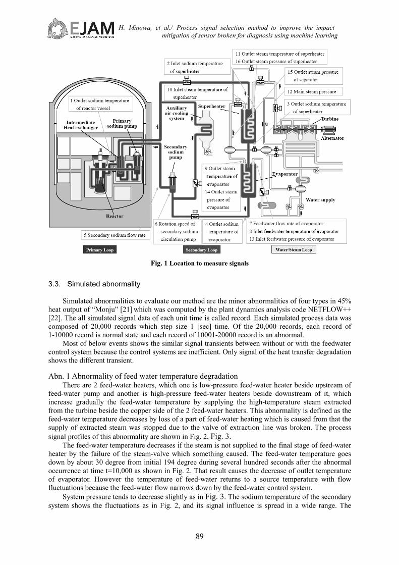
This section explains process signals which were used in evaluation experiment. Our evaluation uses the process signals of the A loop only in every the three loops of the secondary sodium and water/steam in Monju. Signals used in our evaluation shows in Table 1, and location of the sensors to measure signal shows in Fig. 1[20].

Table 1 Name list of signals

No Name of signal

Sig. 1 Outlet sodium temperature of reactor vessel Sig. 2 Inlet sodium temperature of superheater Sig. 3 Outlet sodium temperature of superheater Sig. 4 Outlet sodium temperature of evaporator Sig. 5 Secondary sodium flow rate Sig. 6 Rotation speed of secondary sodium circulation pump Sig. 7 Feedwater flow rate of evaporator Sig. 8 Inlet feedwater temperature of evaporator Sig. 9 Outlet steam temperature of evaporator Sig. 10 Inlet steam temperature of superheater Sig. 11 Outlet steam temperature of superheater Sig. 12 Main steam pressure Sig. 13 Inlet feedwater pressure of evaporator Sig. 14 Outlet steam pressure of evaporator Sig. 15 Outlet steam pressure of separator Sig. 16 Outlet steam pressure of superheater


89

Fig. 1 Location to measure signals

3.3. Simulated abnormality

Simulated abnormalities to evaluate our method are the minor abnormalities of four types in 45% heat output of “Monju” [21] which was computed by the plant dynamics analysis code NETFLOW++ [22]. The all simulated signal data of each unit time is called record. Each simulated process data was composed of 20,000 records which step size 1 [sec] time. Of the 20,000 records, each record of 1-10000 record is normal state and each record of 10001-20000 record is an abnormal.

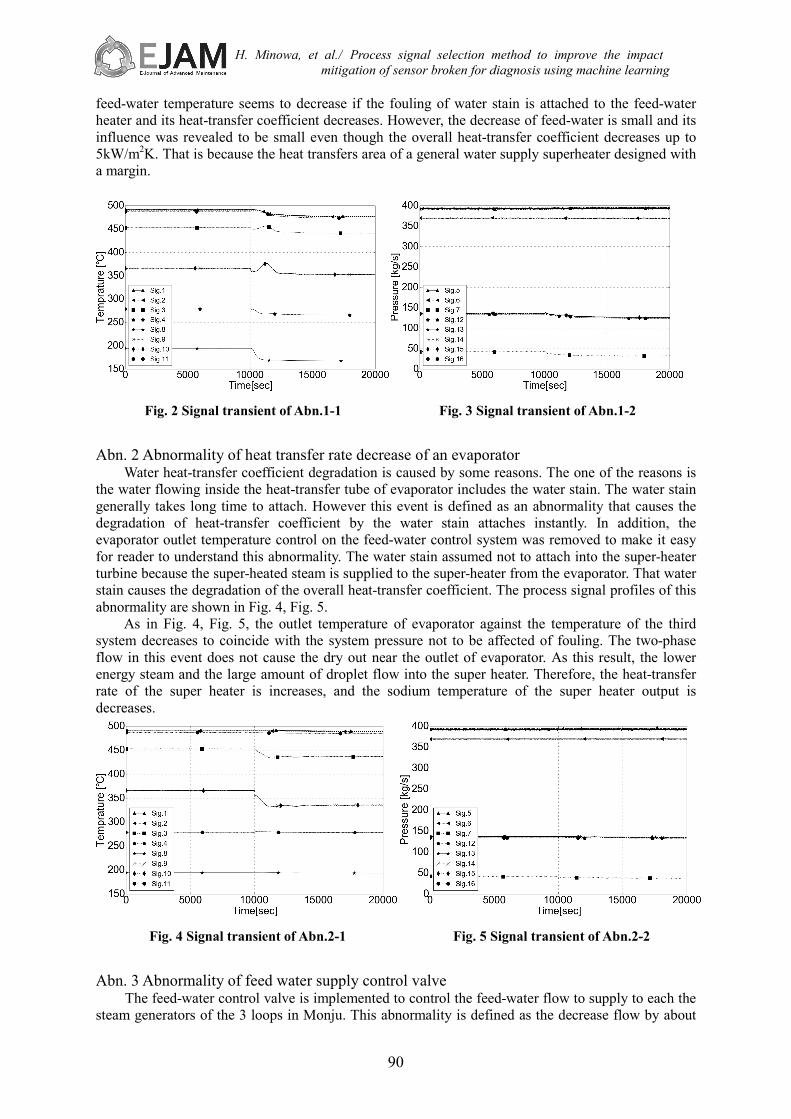
Most of below events shows the similar signal transients between without or with the feedwater control system because the control systems are inefficient. Only signal of the heat transfer degradation shows the different transient. Abn. 1 Abnormality of feed water temperature degradation

There are 2 feed-water heaters, which one is low-pressure feed-water heater beside upstream of feed-water pump and another is high-pressure feed-water heaters beside downstream of it, which increase gradually the feed-water temperature by supplying the high-temperature steam extracted from the turbine beside the copper side of the 2 feed-water heaters. This abnormality is defined as the feed-water temperature decreases by loss of a part of feed-water heating which is caused from that the supply of extracted steam was stopped due to the valve of extraction line was broken. The process signal profiles of this abnormality are shown in Fig. 2, Fig. 3.

The feed-water temperature decreases if the steam is not supplied to the final stage of feed-water heater by the failure of the steam-valve which something caused. The feed-water temperature goes down by about 30 degree from initial 194 degree during several hundred seconds after the abnormal occurrence at time t=10,000 as shown in Fig. 2. That result causes the decrease of outlet temperature of evaporator. However the temperature of feed-water returns to a source temperature with flow fluctuations because the feed-water flow narrows down by the feed-water control system.

System pressure tends to decrease slightly as in Fig. 3. The sodium temperature of the secondary system shows the fluctuations as in Fig. 2, and its signal influence is spread in a wide range. The


90

feed-water temperature seems to decrease if the fouling of water stain is attached to the feed-water heater and its heat-transfer coefficient decreases. However, the decrease of feed-water is small and its influence was revealed to be small even though the overall heat-transfer coefficient decreases up to 5kW/m2K. That is because the heat transfers area of a general water supply superheater designed with a margin.

Fig. 2 Signal transient of Abn.1-1


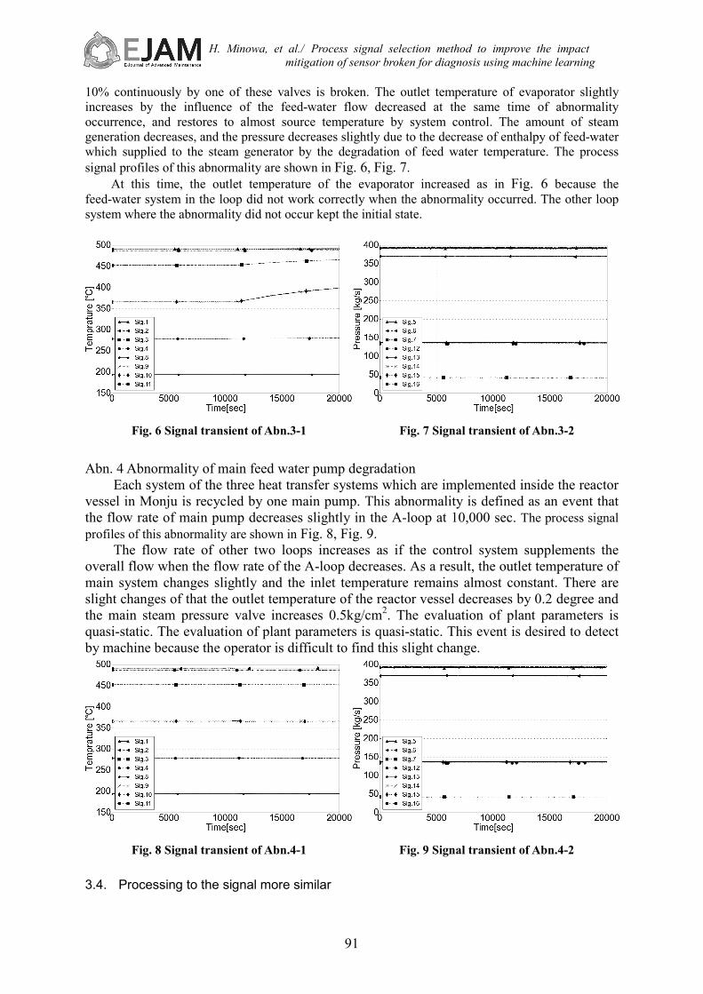
Abn. 2 Abnormality of heat transfer rate decrease of an evaporator

Water heat-transfer coefficient degradation is caused by some reasons. The one of the reasons is the water flowing inside the heat-transfer tube of evaporator includes the water stain. The water stain generally takes long time to attach. However this event is defined as an abnormality that causes the degradation of heat-transfer coefficient by the water stain attaches instantly. In addition, the evaporator outlet temperature control on the feed-water control system was removed to make it easy for reader to understand this abnormality. The water stain assumed not to attach into the super-heater turbine because the super-heated steam is supplied to the super-heater from the evaporator. That water stain causes the degradation of the overall heat-transfer coefficient. The process signal profiles of this abnormality are shown in Fig. 4, Fig. 5.

As in Fig. 4, Fig. 5, the outlet temperature of evaporator against the temperature of the third system decreases to coincide with the system pressure not to be affected of fouling. The two-phase flow in this event does not cause the dry out near the outlet of evaporator. As this result, the lower energy steam and the large amount of droplet flow into the super heater. Therefore, the heat-transfer rate of the super heater is increases, and the sodium temperature of the super heater output is decreases.



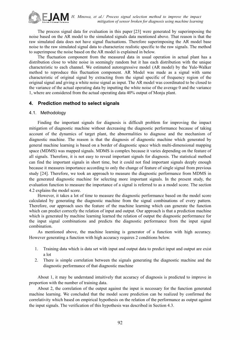
Abn. 3 Abnormality of feed water supply control valve

The feed-water control valve is implemented to control the feed-water flow to supply to each the steam generators of the 3 loops in Monju. This abnormality is defined as the decrease flow by about


91

10% continuously by one of these valves is broken. The outlet temperature of evaporator slightly increases by the influence of the feed-water flow decreased at the same time of abnormality occurrence, and restores to almost source temperature by system control. The amount of steam generation decreases, and the pressure decreases slightly due to the decrease of enthalpy of feed-water which supplied to the steam generator by the degradation of feed water temperature. The process signal profiles of this abnormality are shown in Fig. 6, Fig. 7.

At this time, the outlet temperature of the evaporator increased as in Fig. 6 because the feed-water system in the loop did not work correctly when the abnormality occurred. The other loop system where the abnormality did not occur kept the initial state.



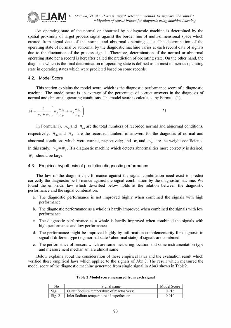
Abn. 4 Abnormality of main feed water pump degradation

Each system of the three heat transfer systems which are implemented inside the reactor vessel in Monju is recycled by one main pump. This abnormality is defined as an event that the flow rate of main pump decreases slightly in the A-loop at 10,000 sec. The process signal profiles of this abnormality are shown in Fig. 8, Fig. 9.

The flow rate of other two loops increases as if the control system supplements the overall flow when the flow rate of the A-loop decreases. As a result, the outlet temperature of main system changes slightly and the inlet temperature remains almost constant. There are slight changes of that the outlet temperature of the reactor vessel decreases by 0.2 degree and the main steam pressure valve increases 0.5kg/cm2. The evaluation of plant parameters is quasi-static. The evaluation of plant parameters is quasi-static. This event is desired to detect by machine because the operator is difficult to find this slight change.



3.4. Processing to the signal more similar


92

The process signal data for evaluation in this paper [23] were generated by superimposing the noise based on the AR model to the simulated signals data mentioned above. That reason is that the raw simulated data does not have signal fluctuations. Therefore superimposing the AR model base noise to the raw simulated signal data to characterize realistic specific to the raw signals. The method to superimpose the noise based on the AR model is explained in below.

The fluctuation component from the measured data in usual operation in actual plant has a distribution close to white noise in seemingly random but it has each distribution with the unique characteristic to each channel. We estimated autoregressive model (AR model) by the Yule-Walker method to reproduce this fluctuation component. AR Model was made as a signal with same characteristic of original signal by extracting from the signal specific of frequency region of the original signal and giving a white noise signal as input. The AR model was coordinated to be closed to the variance of the actual operating data by inputting the white noise of the average 0 and the variance 1, where are considered from the actual operating data 40% output of Monju plant. 4. Prediction method to select signals 4.1. Methodology

Finding the important signals for diagnosis is difficult problem for improving the impact mitigation of diagnostic machine without decreasing the diagnostic performance because of taking account of the dynamics of target plant, the abnormalities to diagnose and the mechanism of diagnostic machine. The reason is that the diagnosis of diagnostic machine which generated by general machine learning is based on a border of diagnostic space which multi-dimensional mapping space (MDMS) was mapped signals. MDMS is complex because it varies depending on the feature of all signals. Therefore, it is not easy to reveal important signals for diagnosis. The statistical method can find the important signals in short time, but it could not find important signals deeply enough because it measures importance according to only the change of feature of single signal from previous study [24]. Therefore, we took an approach to measure the diagnostic performance from MDMS in the generated diagnostic machine for selecting more important signals. In the present study, the evaluation function to measure the importance of a signal is referred to as a model score. The section 4.2 explains the model score.

However, it takes a lot of time to measure the diagnostic performance based on the model score calculated by generating the diagnostic machine from the signal combinations of every pattern. Therefore, our approach uses the feature of the machine learning which can generate the function which can predict correctly the relation of input and output. Our approach is that a prediction machine which is generated by machine learning learned the relation of output the diagnostic performance for the input signal combinations and predicts the diagnostic performance from the input signal combination.

As mentioned above, the machine learning is generator of a function with high accuracy. However generating a function with high accuracy requires 2 conditions below.

1. Training data which is data set with input and output data to predict input and output are exist

a lot 2. There is simple correlation between the signals generating the diagnostic machine and the

diagnostic performance of that diagnostic machine

About 1, it may be understand intuitively that accuracy of diagnosis is predicted to improve in proportion with the number of training data.

About 2, the correlation of the output against the input is necessary for the function generated machine learning. We concluded that the model score prediction can be realized by confirmed the correlativity which based on empirical hypothesis on the relation of the performance as output against the input signals. The verification of this hypothesis was described in Section 4.3.


93

An operating state of the normal or abnormal by a diagnostic machine is determined by the spatial proximity of target process signal against the border line of multi-dimensional space which created from signal data of the normal and abnormal operating state. The determination of the operating state of normal or abnormal by the diagnostic machine varies at each record data of signals due to the fluctuation of the process signals. Therefore, determination of the normal or abnormal operating state per a record is hereafter called the prediction of operating state. On the other hand, the diagnosis which is the final determination of operating state is defined as an most numerous operating state in operating states which were predicted based on some records. 4.2. Model Score

This section explains the model score, which is the diagnostic performance score of a diagnostic machine. The model score is an average of the percentage of correct answers in the diagnosis of normal and abnormal operating conditions. The model score is calculated by Formula (1).

+

+=

Sa

Aaa

Sn

Ann

an nn

wnn

www

M 1 (1)

In Formula(1), Snn and San are the total numbers of recorded normal and abnormal conditions,

respectively; Ann and Aan are the recorded numbers of answers for the diagnosis of normal and

abnormal conditions which were correct, respectively; and nw and aw are the weight coefficients.

In this study, nw = aw . If a diagnostic machine which detects abnormalities more correctly is desired,

aw should be large. 4.3. Empirical hypothesis of prediction diagnostic performance

The law of the diagnostic performance against the signal combination need exist to predict correctly the diagnostic performance against the signal combination by the diagnostic machine. We found the empirical law which described below holds at the relation between the diagnostic performance and the signal combination.

a. The diagnostic performance is not improved highly when combined the signals with high performance

b. The diagnostic performance as a whole is hardly improved when combined the signals with low performance

c. The diagnostic performance as a whole is hardly improved when combined the signals with high performance and low performance

d. The performance might be improved highly by information complementarity for diagnosis in signal if different type (e.g. normal state / abnormal state) of signals are combined

e. The performance of sensors which are same measuring location and same instrumentation type and measurement mechanism are almost same

Below explains about the consideration of these empirical laws and the evaluation result which verified these empirical laws which applied to the signals of Abn.3. The result which measured the model score of the diagnostic machine generated from single signal in Abn3 shows in Table2.

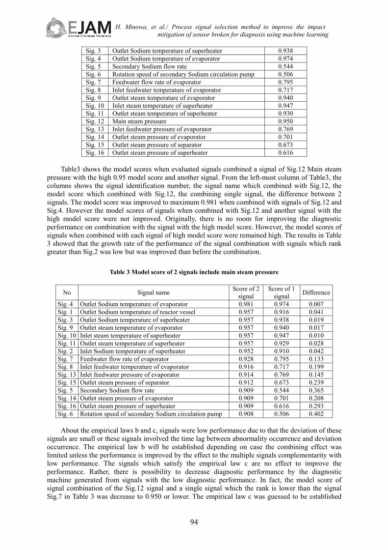
Table 2 Model score measured from each signal

No Signal name Model Score Sig. 1 Outlet Sodium temperature of reactor vessel 0.916 Sig. 2 Inlet Sodium temperature of superheater 0.910


94

Sig. 3 Outlet Sodium temperature of superheater 0.938 Sig. 4 Outlet Sodium temperature of evaporator 0.974 Sig. 5 Secondary Sodium flow rate 0.544 Sig. 6 Rotation speed of secondary Sodium circulation pump 0.506 Sig. 7 Feedwater flow rate of evaporator 0.795 Sig. 8 Inlet feedwater temperature of evaporator 0.717 Sig. 9 Outlet steam temperature of evaporator 0.940 Sig. 10 Inlet steam temperature of superheater 0.947 Sig. 11 Outlet steam temperature of superheater 0.930 Sig. 12 Main steam pressure 0.950 Sig. 13 Inlet feedwater pressure of evaporator 0.769 Sig. 14 Outlet steam pressure of evaporator 0.701 Sig. 15 Outlet steam pressure of separator 0.673 Sig. 16 Outlet steam pressure of superheater 0.616

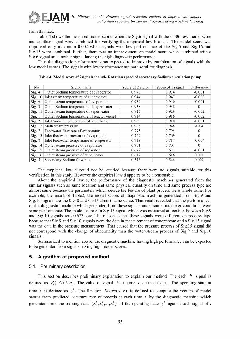
Table3 shows the model scores when evaluated signals combined a signal of Sig.12 Main steam

pressure with the high 0.95 model score and another signal. From the left-most column of Table3, the columns shows the signal identification number, the signal name which combined with Sig.12, the model score which combined with Sig.12, the combining single signal, the difference between 2 signals. The model score was improved to maximum 0.981 when combined with signals of Sig.12 and Sig.4. However the model scores of signals when combined with Sig.12 and another signal with the high model score were not improved. Originally, there is no room for improving the diagnostic performance on combination with the signal with the high model score. However, the model scores of signals when combined with each signal of high model score were remained high. The results in Table 3 showed that the growth rate of the performance of the signal combination with signals which rank greater than Sig.2 was low but was improved than before the combination.

Table 3 Model score of 2 signals include main steam pressure

No Signal name Score of 2

signal Score of 1

signal Difference

Sig. 4 Outlet Sodium temperature of evaporator 0.981 0.974 0.007 Sig. 1 Outlet Sodium temperature of reactor vessel 0.957 0.916 0.041 Sig. 3 Outlet Sodium temperature of superheater 0.957 0.938 0.019 Sig. 9 Outlet steam temperature of evaporator 0.957 0.940 0.017 Sig. 10 Inlet steam temperature of superheater 0.957 0.947 0.010 Sig. 11 Outlet steam temperature of superheater 0.957 0.929 0.028 Sig. 2 Inlet Sodium temperature of superheater 0.952 0.910 0.042 Sig. 7 Feedwater flow rate of evaporator 0.928 0.795 0.133 Sig. 8 Inlet feedwater temperature of evaporator 0.916 0.717 0.199 Sig. 13 Inlet feedwater pressure of evaporator 0.914 0.769 0.145 Sig. 15 Outlet steam pressure of separator 0.912 0.673 0.239 Sig. 5 Secondary Sodium flow rate 0.909 0.544 0.365 Sig. 14 Outlet steam pressure of evaporator 0.909 0.701 0.208 Sig. 16 Outlet steam pressure of superheater 0.909 0.616 0.293 Sig. 6 Rotation speed of secondary Sodium circulation pump 0.908 0.506 0.402

About the empirical laws b and c, signals were low performance due to that the deviation of these

signals are small or these signals involved the time lag between abnormality occurrence and deviation occurrence. The empirical law b will be established depending on case the combining effect was limited unless the performance is improved by the effect to the multiple signals complementarity with low performance. The signals which satisfy the empirical law c are no effect to improve the performance. Rather, there is possibility to decrease diagnostic performance by the diagnostic machine generated from signals with the low diagnostic performance. In fact, the model score of signal combination of the Sig.12 signal and a single signal which the rank is lower than the signal Sig.7 in Table 3 was decrease to 0.950 or lower. The empirical law c was guessed to be established


95

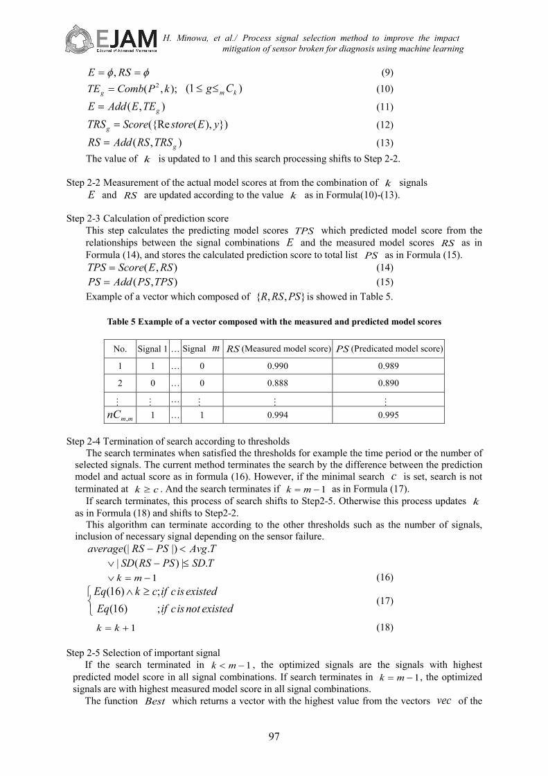
from this fact. Table 4 shows the measured model scores when the Sig.6 signal with the 0.506 low model score

and another signal were combined for verifying the empirical law b and c. The model score was improved only maximum 0.002 when signals with low performance of the Sig.5 and Sig.16 and Sig.15 were combined. Further, there was no improvement on model score when combined with a Sig.6 signal and another signal having the high diagnostic performance.

Thus the diagnostic performance is not expected to improve by combination of signals with the low model scores. The signals with low performance are not useful for diagnosis.

Table 4 Model score of 2signals include Rotation speed of secondary Sodium circulation pump

No Signal name Score of 2 signal Score of 1 signal Difference Sig. 4 Outlet Sodium temperature of evaporator 0.973 0.974 -0.001 Sig. 10 Inlet steam temperature of superheater 0.944 0.947 -0.003 Sig. 9 Outlet steam temperature of evaporator 0.939 0.940 -0.001 Sig. 3 Outlet Sodium temperature of superheater 0.938 0.938 0 Sig. 11 Outlet steam temperature of superheater 0.927 0.929 -0.002 Sig. 1 Outlet Sodium temperature of reactor vessel 0.914 0.916 -0.002 Sig. 2 Inlet Sodium temperature of superheater 0.909 0.910 -0.001 Sig. 12 Main steam pressure 0.908 0.948 -0.04 Sig. 7 Feedwater flow rate of evaporator 0.795 0.795 0 Sig. 13 Inlet feedwater pressure of evaporator 0.769 0.769 0 Sig. 8 Inlet feedwater temperature of evaporator 0.713 0.717 -0.004 Sig. 14 Outlet steam pressure of evaporator 0.701 0.701 0 Sig. 15 Outlet steam pressure of separator 0.672 0.673 -0.001 Sig. 16 Outlet steam pressure of superheater 0.617 0.616 0.001 Sig. 5 Secondary Sodium flow rate 0.546 0.544 0.002

The empirical law d could not be verified because there were no signals suitable for this

verification in this study. However the empirical law d appears to be a reasonable. About the empirical law e, the performance of the diagnostic machines generated from the

similar signals such as same location and same physical quantity on time and same process type are almost same because the parameters which decide the feature of plant process were whole same. For example, the result of Table2, the model scores of diagnostic machine generated from Sig.9 and Sig.10 signals are the 0.940 and 0.947 almost same value. That result revealed that the performances of the diagnostic machine which generated from these signals under same parameter conditions were same performance. The model score of a Sig.15 signal which was measured at location between Sig.9 and Sig.10 signals was 0.673 low. The reason is that these signals were different on process type because that Sig.9 and Sig.10 signals were the data in measurement of water/steam and a Sig.15 signal was the data in the pressure measurement. That caused that the pressure process of Sig.15 signal did not correspond with the change of abnormality than the water/stream process of Sig.9 and Sig.10 signals.

Summarized to mention above, the diagnostic machine having high performance can be expected to be generated from signals having high model scores. 5. Algorithm of proposed method 5.1. Preliminary description

This section describes preliminary explanation to explain our method. The each n signal is defined as )1( niPi ≤≤ . The value of signal iP at time t defined as t

ix . The operating state at

time t is defined as ty . The function ),( yxScore is defined to compute the vectors of model scores from predicted accuracy rate of records at each time t by the diagnostic machine which generated from the training data ),...,,( 21

ti

tt xxx of the operating state ty against each signal of i


96

species. The total number of signal combinations selected all signal up to l−1 from m signals is described as in Formula (2). Thus the all signal combinations is defined as mmnC , .

∑ ==

l

b bmlm CnC1, )( (2)

The unit element e has a value of 0/1. The value of ie is 1 if signal i is exists in a signal combination. The value is 0 if signal i is not. The function is defined as in Formula (3).

=existnotisisignalif

existisisignalifei ,0

,1 (3)

The function Comb is the function returns a vector which is the signal combinations u which composed of the unit element e in the ik C signal combinations which composed of the i signals selected from the k signals of P . The function is defined as in Formula (4).

);,...,,(),( ,2,1, kuuu eeeiPComb = )1( ik Cu≤≤ (4) The function storeRe , is defined as in Formula (5), is the function returns the vector of the

signal data which restored according to the values of element e in the vector u in the signal combination E composed of the n unit element e .

}),...,{(;,...,)(Re ,1,,1,1 nuuununuu eeEexexEstore == (5) The ),( qpAdd function adds vector q to the tail of vector p .

5.2. Algorithm Step 1 Screening of signals Step 1-1 Calculation of base model score

The base model score BS as a threshold to select signals is calculated as in Formula (6).

),( yxScoreS B = (6) Step 1-2 Calculation of model scores of each signal

The model scores of each signal are calculated as in Formula (7). ),( yxScoreS ii = (7)

Step 1-3 Selection of signal

The important signal candidates )1(2 mjPj ≤≤ are selected as in Formula (8).

The Formula (8) indicates to select the signals 2jP , which has the model score more than the

base model score BS , or the rank is greater than equal to b , from the signals iS .

)}(|{ 2iiBj SOrderbSSP ≥∨≤ (8)

Step 2 Selection of the signals considering the signal combinations Step 2-1 Measurement of the actual model score from the combination of m all signals

The model scores which evaluated the signal combination which composed of the selected c signals are calculated as in Formula (9)-(13).

A signal selection number k is initialized at m . The signal combinations E and model scores RS of each record are initialized as in formula (9). The vector TE is composed of the g unit element e representing the signal combination which selected the m signals from

signals 2P . The vector TE is calculated as in formula (10), (11). The vector TE is stored to the tail of E .

The model scores gTRS were calculated from E as in Formula (12), and stored to RS as in (13).


97

φφ == RSE , (9) );,( 2 kPCombTEg = )1( km Cg≤≤ (10)

),( gTEEAddE = (11)

})),(({Re yEstoreScoreTRSg = (12)

),( gTRSRSAddRS = (13) The value of k is updated to 1 and this search processing shifts to Step 2-2.

Step 2-2 Measurement of the actual model scores at from the combination of k signals

E and RS are updated according to the value k as in Formula(10)-(13). Step 2-3 Calculation of prediction score

This step calculates the predicting model scores TPS which predicted model score from the relationships between the signal combinations E and the measured model scores RS as in Formula (14), and stores the calculated prediction score to total list PS as in Formula (15).

),( RSEScoreTPS = (14) ),( TPSPSAddPS = (15)

Example of a vector which composed of },,{ PSRSR is showed in Table 5.

Table 5 Example of a vector composed with the measured and predicted model scores

No. Signal 1 … Signal m RS (Measured model score) PS (Predicated model score)

1 1 … 0 0.990 0.989

2 0 … 0 0.888 0.890

…

… … …

…

…

mmnC , 1 … 1 0.994 0.995 Step 2-4 Termination of search according to thresholds

The search terminates when satisfied the thresholds for example the time period or the number of selected signals. The current method terminates the search by the difference between the prediction model and actual score as in formula (16). However, if the minimal search c is set, search is not terminated at ck ≥ . And the search terminates if 1−= mk as in Formula (17).

If search terminates, this process of search shifts to Step2-5. Otherwise this process updates k as in Formula (18) and shifts to Step2-2.

This algorithm can terminate according to the other thresholds such as the number of signals, inclusion of necessary signal depending on the sensor failure.

TAvgPSRSaverage .|)(| <− TSDPSRSSD .|)(| ≤−∨ 1−=∨ mk (16)

≥∧

existednotiscifEqexistediscifckEq

;)16(;)16(

(17)

1+= kk (18)

Step 2-5 Selection of important signal If the search terminated in 1−< mk , the optimized signals are the signals with highest

predicted model score in all signal combinations. If search terminates in 1−= mk , the optimized signals are with highest measured model score in all signal combinations.

The function Best which returns a vector with the highest value from the vectors vec of the


98

measured model scores or the predicted model scores is defined as in the formula (19).

−==−<=

=1;1;

)(mkifRSvecmkifPSvec

vecBestsignalsBest (19)

6. Evaluation Experiment 6.1. Evaluation of prediction performance

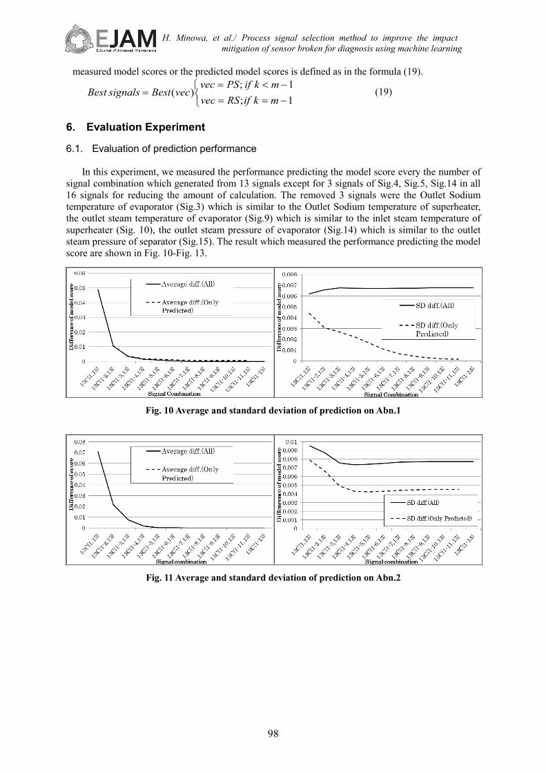
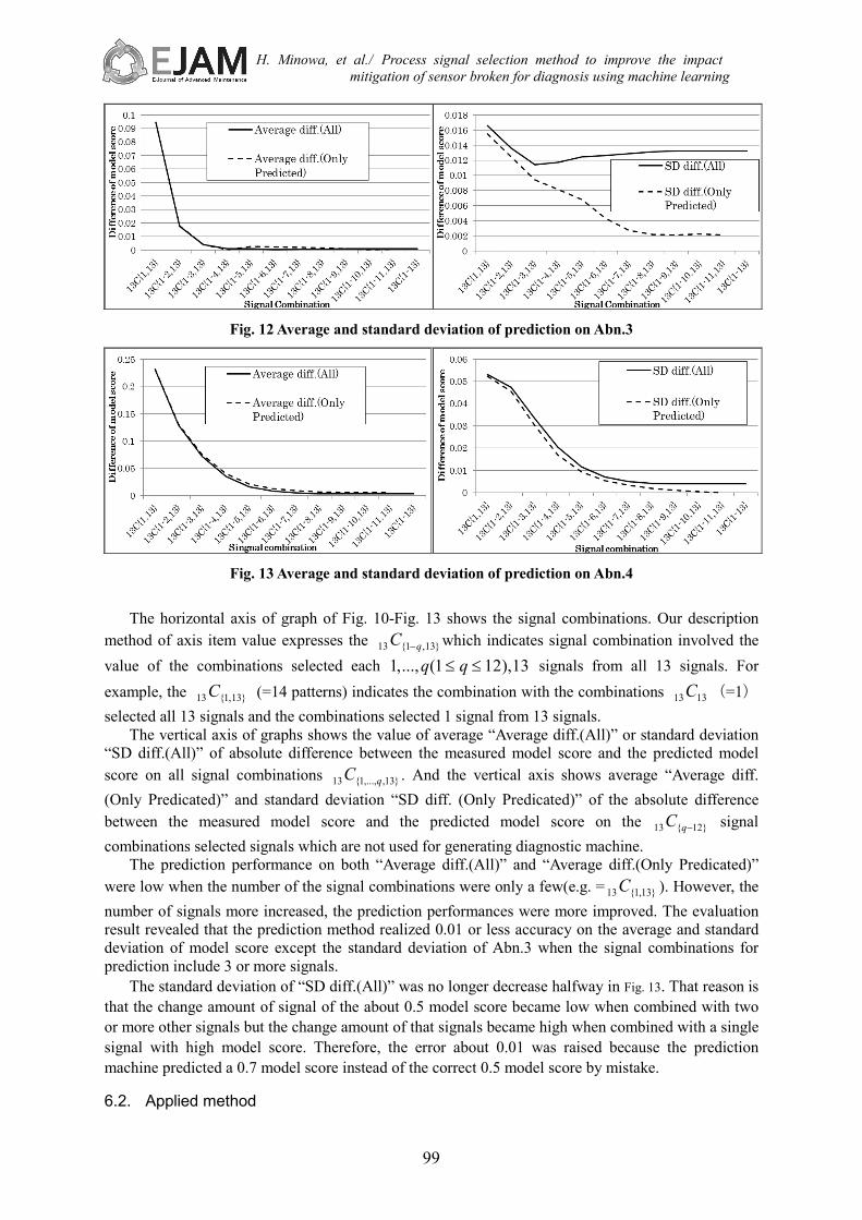
In this experiment, we measured the performance predicting the model score every the number of signal combination which generated from 13 signals except for 3 signals of Sig.4, Sig.5, Sig.14 in all 16 signals for reducing the amount of calculation. The removed 3 signals were the Outlet Sodium temperature of evaporator (Sig.3) which is similar to the Outlet Sodium temperature of superheater, the outlet steam temperature of evaporator (Sig.9) which is similar to the inlet steam temperature of superheater (Sig. 10), the outlet steam pressure of evaporator (Sig.14) which is similar to the outlet steam pressure of separator (Sig.15). The result which measured the performance predicting the model score are shown in Fig. 10-Fig. 13.

Fig. 10 Average and standard deviation of prediction on Abn.1



99



The horizontal axis of graph of Fig. 10-Fig. 13 shows the signal combinations. Our description

method of axis item value expresses the }13,1{13 qC − which indicates signal combination involved the value of the combinations selected each 13),121(...,,1 ≤≤ qq signals from all 13 signals. For example, the }13,1{13C (=14 patterns) indicates the combination with the combinations 1313C （=1） selected all 13 signals and the combinations selected 1 signal from 13 signals.

The vertical axis of graphs shows the value of average “Average diff.(All)” or standard deviation “SD diff.(All)” of absolute difference between the measured model score and the predicted model score on all signal combinations }13,,...,1{13 qC . And the vertical axis shows average “Average diff. (Only Predicated)” and standard deviation “SD diff. (Only Predicated)” of the absolute difference between the measured model score and the predicted model score on the }12{13 −qC signal combinations selected signals which are not used for generating diagnostic machine.

The prediction performance on both “Average diff.(All)” and “Average diff.(Only Predicated)” were low when the number of the signal combinations were only a few(e.g. = }13,1{13C ). However, the number of signals more increased, the prediction performances were more improved. The evaluation result revealed that the prediction method realized 0.01 or less accuracy on the average and standard deviation of model score except the standard deviation of Abn.3 when the signal combinations for prediction include 3 or more signals.

The standard deviation of “SD diff.(All)” was no longer decrease halfway in Fig. 13. That reason is that the change amount of signal of the about 0.5 model score became low when combined with two or more other signals but the change amount of that signals became high when combined with a single signal with high model score. Therefore, the error about 0.01 was raised because the prediction machine predicted a 0.7 model score instead of the correct 0.5 model score by mistake. 6.2. Applied method


100

Our method was applied to the signal data “Monju” for evaluating the diagnostic accuracy and

the early detection. Step1 screens out the effective less signals from all 16 signals. The threshold b to select signals was set 8 in this evaluation. So this search process selected the 8 signals with higher the model score because there was no signal iP which the model score was more than BS . And it proceeds to Step2. Step2 analyzed the remained signals with the parameter 001.0. =TAvg ,

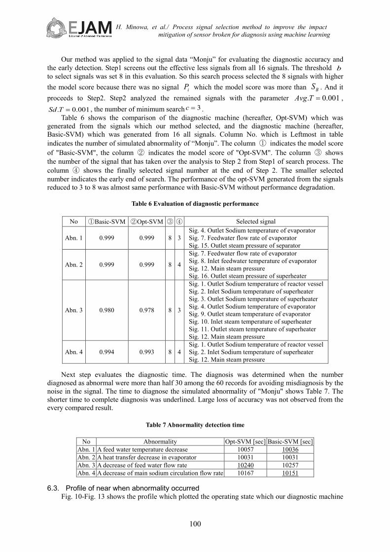
001.0. =TSd , the number of minimum search 3=c . Table 6 shows the comparison of the diagnostic machine (hereafter, Opt-SVM) which was

generated from the signals which our method selected, and the diagnostic machine (hereafter, Basic-SVM) which was generated from 16 all signals. Column No. which is Leftmost in table indicates the number of simulated abnormality of “Monju”. The column ① indicates the model score of "Basic-SVM", the column ② indicates the model score of "Opt-SVM". The column ③ shows the number of the signal that has taken over the analysis to Step 2 from Step1 of search process. The column ④ shows the finally selected signal number at the end of Step 2. The smaller selected number indicates the early end of search. The performance of the opt-SVM generated from the signals reduced to 3 to 8 was almost same performance with Basic-SVM without performance degradation.

Table 6 Evaluation of diagnostic performance

No ①Basic-SVM ②Opt-SVM ③ ④ Selected signal

Abn. 1 0.999 0.999 8 3 Sig. 4. Outlet Sodium temperature of evaporator Sig. 7. Feedwater flow rate of evaporator Sig. 15. Outlet steam pressure of separator

Abn. 2 0.999 0.999 8 4

Sig. 7. Feedwater flow rate of evaporator Sig. 8. Inlet feedwater temperature of evaporator Sig. 12. Main steam pressure Sig. 16. Outlet steam pressure of superheater

Abn. 3 0.980 0.978 8 3

Sig. 1. Outlet Sodium temperature of reactor vessel Sig. 2. Inlet Sodium temperature of superheater Sig. 3. Outlet Sodium temperature of superheater Sig. 4. Outlet Sodium temperature of evaporator Sig. 9. Outlet steam temperature of evaporator Sig. 10. Inlet steam temperature of superheater Sig. 11. Outlet steam temperature of superheater Sig. 12. Main steam pressure

Abn. 4 0.994 0.993 8 4 Sig. 1. Outlet Sodium temperature of reactor vessel Sig. 2. Inlet Sodium temperature of superheater Sig. 12. Main steam pressure

Next step evaluates the diagnostic time. The diagnosis was determined when the number

diagnosed as abnormal were more than half 30 among the 60 records for avoiding misdiagnosis by the noise in the signal. The time to diagnose the simulated abnormality of "Monju" shows Table 7. The shorter time to complete diagnosis was underlined. Large loss of accuracy was not observed from the every compared result.

Table 7 Abnormality detection time

No Abnormality Opt-SVM [sec] Basic-SVM [sec] Abn. 1 A feed water temperature decrease 10057 10036 Abn. 2 A heat transfer decrease in evaporator 10031 10031 Abn. 3 A decrease of feed water flow rate 10240 10257 Abn. 4 A decrease of main sodium circulation flow rate 10167 10151

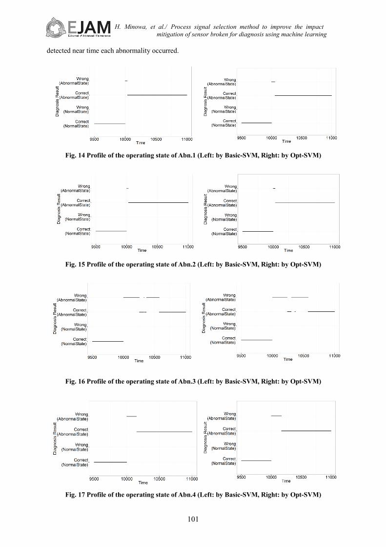
6.3. Profile of near when abnormality occurred

Fig. 10-Fig. 13 shows the profile which plotted the operating state which our diagnostic machine


101

detected near time each abnormality occurred.

Fig. 14 Profile of the operating state of Abn.1 (Left: by Basic-SVM, Right: by Opt-SVM)





102

In Fig. 14-Fig. 17, The horizontal axes show the diagnostic time, and the vertical axes show each

operating states from top is that “Correct (Abnormal State)” was plotted when diagnosis were correct in abnormal state, “Wrong (Abnormal State)” was plotted when diagnosis were wrong in abnormal state, “Wrong (Abnormal State)” was plotted when diagnosis were wrong in abnormal state, “Correct (Normal State)” was plotted when diagnosis were wrong in normal state. The diagnostic results of both the Opt-SVM and the Basic-SVM were visually confirmed the same from these profiles. 6.4. Comparing with the other method

This section shows the result compared with other method as sensitivity analysis method [17] and F-Score Method [14]. The number selecting signals in these comparing methods was set the same number of our method because there is no description of the algorithm to terminate the search.

The sensitivity analysis method could not calculate the score in many signals. The model score that could be carried out the procedure to select signals of Abn.3 was 0.974. The model score of the Opt-SVM of same Abn.3 was 0.978 is higher by 0.4%. The reason was guessed that the just created diagnostic machine diagnosed with the either normal or abnormal operating states from the every records of training data which averaged of each variable except one variable. As a result, the sensitivity analysis method could not compute the selecting score because the standard deviation became zero at a single regression analysis.

The compared result of the each model score calculated from our selection method and the F-Score method shows in Table 8. The Table 8 revealed that the model score of the proposed method was slightly better or equal to the F-Score method.

Table 8 Comparison with F-Score method

Abn Score Selected signals

Opt-SVM F-Score method (Score order)

1 0.999 0.998 Sig. 4 Outlet Sodium temperature of evaporator Sig. 7 Feedwater flow rate of evaporator Sig. 8 Inlet feedwater temperature of evaporator

2 0.999 0.999

Sig. 3 Outlet Sodium temperature of superheater, Sig. 7 Feedwater flow rate of evaporator Sig. 9 Outlet steam temperature of evaporator Sig.10 Inlet steam temperature of superheater

3 0.978 0.975

Sig. 1 Outlet Sodium temperature of reactor vessel Sig. 2 Inlet Sodium temperature of superheater Sig. 3 Outlet Sodium temperature of superheater Sig. 4 Outlet Sodium temperature of evaporator Sig. 7 Feedwater flow rate of evaporator Sig. 9 Outlet steam temperature of evaporator Sig.10 Inlet steam temperature of superheater Sig.11 Outlet steam temperature of superheater

4 0.993 0.993 Sig. 1 Outlet Sodium temperature of reactor vessel Sig. 2 Inlet Sodium temperature of superheater Sig. 12 Main steam pressure

6.5. Discussion

The result in chapter 6.1 which evaluated the prediction performance of our method revealed that our method could predict model scores of each signal combination correctly. For example the predicting accuracy of average and standard deviation were 0.01 or less, when training data was composed of signals from 3 to 4.

The evaluation result in chapter 6.2 revealed that the performance and the diagnostic time were


103

almost same when our method reduced to 3-8 a number of signals of training data. The reason is that the difference of performance was 0-0.02 or less and the delay of the diagnosed time was within seconds from -17 to 16.

The diagnosed profiles which applied our method in chapter 6.3 were confirmed visually the same with the diagnosed profile which generated by general machine learning of time near the abnormality occurs. The mentioned results which applied our method were same accuracy despite of reducing the number of signals to generate the diagnostic machine. That indicates that the diagnostic machine which applied our method can continue to diagnose with same accuracy even if data of a part of signals are not obtained.

The result compared with the sensitivity analysis method and F-Score method in chapter 6.4 revealed that our method improved of 0-0.3% than both methods.

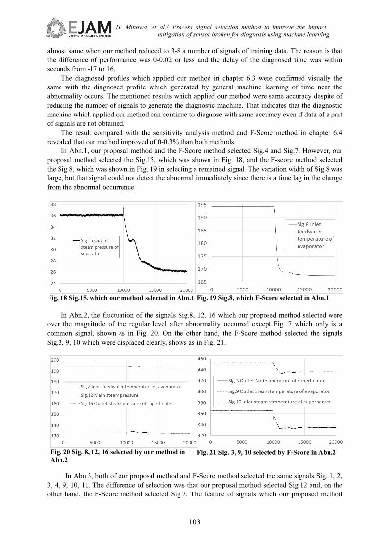
In Abn.1, our proposal method and the F-Score method selected Sig.4 and Sig.7. However, our proposal method selected the Sig.15, which was shown in Fig. 18, and the F-score method selected the Sig.8, which was shown in Fig. 19 in selecting a remained signal. The variation width of Sig.8 was large, but that signal could not detect the abnormal immediately since there is a time lag in the change from the abnormal occurrence.

Fig. 18 Sig.15, which our method selected in Abn.1

Fig. 19 Sig.8, which F-Score selected in Abn.1

In Abn.2, the fluctuation of the signals Sig.8, 12, 16 which our proposed method selected were

over the magnitude of the regular level after abnormality occurred except Fig. 7 which only is a common signal, shown as in Fig. 20. On the other hand, the F-Score method selected the signals Sig.3, 9, 10 which were displaced clearly, shows as in Fig. 21.

Fig. 20 Sig. 8, 12, 16 selected by our method in Abn.2

Fig. 21 Sig. 3, 9, 10 selected by F-Score in Abn.2

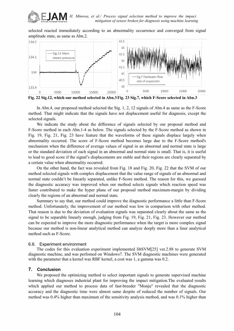
In Abn.3, both of our proposal method and F-Score method selected the same signals Sig. 1, 2,

3, 4, 9, 10, 11. The difference of selection was that our proposal method selected Sig.12 and, on the other hand, the F-Score method selected Sig.7. The feature of signals which our proposed method


104

selected reacted immediately according to an abnormality occurrence and converged from signal amplitude state, as same as Abn.2.

Fig. 22 Sig.12, which our method selected in Abn.3

Fig. 23 Sig.7, which F-Score selected in Abn.3

In Abn.4, our proposed method selected the Sig. 1, 2, 12 signals of Abn.4 as same as the F-Score

method. That might indicate that the signals have not displacement useful for diagnosis, except the selected signals.

We indicate the study about the difference of signals selected by our proposal method and F-Score method in each Abn.1-4 as below. The signals selected by the F-Score method as shown in Fig. 19, Fig. 21, Fig. 23 have feature that the waveforms of these signals displace largely when abnormality occurred. The score of F-Score method becomes large due to the F-Score method's mechanism when the difference of average values of signal in an abnormal and normal state is large or the standard deviation of each signal in an abnormal and normal state is small. That is, it is useful to lead to good score if the signal’s displacements are stable and their regions are clearly separated by a certain value when abnormality occurred.

On the other hand, the fact was revealed from Fig. 18 and Fig. 20, Fig. 22 that the SVM of our method selected signals with complex displacement that the value range of signals of an abnormal and normal state couldn’t be linearly separated, unlike F-Score method. The reason for this, we guessed the diagnostic accuracy was improved when our method selects signals which reaction speed was faster contributed to make the hyper plane of our proposal method maximum-margin by dividing clearly the regions of an abnormal and normal state.

Summary to say that, our method could improve the diagnostic performance a little than F-Score method. Unfortunately, the improvement of our method was low in comparison with other method. That reason is due to the deviation of evaluation signals was separated clearly about the same as the signal to be separable linearly enough, judging from Fig. 19, Fig. 21, Fig. 23. However our method can be expected to improve the more diagnostic performance when the target is more complex signal because our method is non-linear analytical method can analyze deeply more than a liner analytical method such as F-Score. 6.6. Experiment environment

The codes for this evaluation experiment implemented libSVM[25] ver.2.88 to generate SVM diagnostic machine, and was perfomed on Windows7. The SVM diagnostic machines were generated with the parameter that a kernel was RBF kernel, a cost was 1, a gamma was 0.2. 7. Conclusion

We proposed the optimizing method to select important signals to generate supervised machine learning which diagnoses industrial plant for improving the impact mitigation.The evaluated results which applied our method to process data of fast-breeder "Monju" revealed that the diagnostic accuracy and the diagnostic time were almost same despite of reduced the number of signals. Our method was 0.4% higher than maximum of the sensitivity analysis method, and was 0.1% higher than


105

maximum of the F-Score method. The improvement were low because the evaluated process data might be simple.

In future works, we propose a diagnostic method using this proposed method to diagnose correctly similar abnormality in virtual plant in which various abnormalities occurs.

Acknowledgement This present study includes some of the results of “Anomaly detection agents by advanced hybrid

processing of Monju process data” entrusted to Okayama University by the Ministry of Education, Culture, Sports, Science and Technology of Japan (MEXT). The authors are grateful to Japan Atomic Energy Agency for providing the observed data of Monju. The authors would like to thank Prof. Hiroyasu Mochizuki of Fukui University and Prof. Makoto Takahashi of Tohoku University for providing the simulated data of Monju with artificial noises.

References [1] A. Widodo, B. Yang : “Support vector machine in machine condition monitoring and fault diagnosis,”

Mechanical Systems and Signal Processing, vol. 21, no. 6, pp. 2560–2574, (2007) [2] V. N. Vapnik, Statistical Learning Theory, Wiley Interscience, (1998) [3] D. E. Rumelhart, G. E. Hinton, and R. J. Williams, “Learning representations by back-propagating errors,”

Nature, vol. 323, no. 6088, pp. 533–536, (1986) [4] Y. Xu, L. Wang : “Fault diagnosis system based on rough set theory and support vector machine”, Lecture

Notes in Artificial Intelligence 3614, pp. 980–988 (2005) [5] S. J. Qin : “Survey on data-driven industrial process monitoring and diagnosis”, Annual Reviews in

Control, Vol. 36, No. 2, pp 220-234 (2012) [6] H. Han, B. Gu, T. Wang, Z.R. Li : “Important sensors for chiller fault detection and diagnosis (FDD) from

the perspective of feature selection and machine learning”, International Journal of Refrigeration, Vol 34, No 2, pp. 586-599, (2011)

[7] I. Monroy, R. Benitez, G. Escudero, and M. Graells : “Enhanced plant fault diagnosis based on the characterization of transient stages,” Computers & Chemical Engineering, vol. 37, pp. 200–213 (2012)

[8] S. Ardi, H. Minowa, K. Suzuki : “Detection of Runaway Reaction in a Polyvinyl Chloride Batch Process Using Artificial Neural Networks,” International Journal of Performability Engineering, vol. 5, no. 4, pp. 367 – 376 (2009)

[9] Z. Hu, Y. Cai, X. He, X. Xu : “Fusion of multi-class support vector machine for fault diagnosis”, in: Proceedings of the American Control Conference, pp. 1941–1945 (2005)

[10] H. Hoffmann, M. D. Howard, and M. J. Daily, “Fast pattern matching with time-delay neural networks,” 2011 Int. Jt. Conf. Neural Networks, pp. 2424–2429, (2011).

[11] H. Schwenk and J. Gauvain, “Training Neural Network Language Models,” in Joint Conference HLT/EMNLP, pp. 201–208, (2005).

[12] T. Joachims, “Training linear SVMs in linear time,” in Proceedings of the 12th ACM SIGKDD international conference on Knowledge discovery and data mining - KDD ’06, pp. 217–226, (2006).

[13] B. Huberman and S. H. Clearwater, A Multi-Agent System for Controlling and Building Environments, A Survey of Programming Languages and Platforms for Multi-Agent Systems, pp. 171–176 (1995).

[14] Y.-W. Chen, C.-J. Lin : “Combining SVMs with various feature selection strategies”, http://www.csie.ntu.edu.tw/~cjlin/papers/features.pdf, accessed at May 25, 2009.

[15] H. Tomoyuki, N. Masashi, M. Mitsunorin, Y. Hisatake, “SVM Training Data Selection Using Multi-Objective Genetic Algorithm”, MPS, No. 126, pp. 77–80 (2008) (in Japanese)

[16] C. Huang and C. Wang : “A GA-based feature selection and parameters optimization for support vector machines,” Expert Systems with Applications, vol. 31, no. 2, pp. 231–240 (2006)

[17] K. Tanabe, K. Nishida and T. Suzuki, “Prediction of Carcinogenicity of Chemical Substances with Support Vector Machine”, Journal of Computer Chemistry, Japan, vol. 10, no. 4, pp. 115–121 (2011) (in Japanese)

[18] H. Chang, A. Kong, and L. Haizhou : “An SVM Kernel With GMM-Supervector Based on the Bhattacharyya Distance for Speaker Recognition,” IEEE Signal Processing Letters, vol. 16, no. 1, pp. 49–52, (2009)

[19] K. Aoki, S. Kuroda and M. Kugler et al. : “Feature Selection Using Confident Margin for SVM”, Journal of the Institute of Electronics, Information and Communication Engineers (D-II), No.12, pp. 2291-2300 (2012) (in Japanese)

[20] H. Furusawa and A. Gofuku, “Diagnosis of steam generator by estimating an unobserved important state


106

variable,” J. Nucl. Sci. Technol., vol. 50, no. 9, pp. 942–949, (2013) [21] H. Mochizuki, “Abnormality Transient Analysis of Monju using a Plant System Code”, Proc. in meeting of

Japan Society of Maintenology, 558-563 (2013) (in Japanese) [22] H. Mochizuki : “Development of the plant dynamics analysis code NETFLOW++”, Nuclear Engineering

and Design, 240, pp. 577-587 (2010) [23] N. Takahashi, A. Gofuku, H. Mochizuki, “Anomaly Diagnosis based on Multi-attribute Similarity” , Proc.

in meeting of Japan Society of Maintenology, pp. 553–557 (2013) (in Japanese) [24] H. Minowa, Y. Munesawa, Y. Furuta, A. Gofuku, Method of Selecting Process Signals for Creating

Diagnostic Machines Optimised to Detect Abnormalities in a Plant Using a Support Vector Machine, Chemical Engineering Transactions, Vol. 36, pp.205-210, 2014.

[25] C-C. Chang, C-J. Lin : “LIBSVM – A Library for Support Vector Machines”. http://www.csie.ntu.edu.tw/~cjlin/libsvm/, Accessed at 13.09.24.

Documents

Process signal selection method to improve the impact ... · broken for diagnosis using machine learning . ... in comparison with the basic diagnostic machine which ... simulated