Process Scheduling

Dr. Yingwu Zhu

Process Behavior

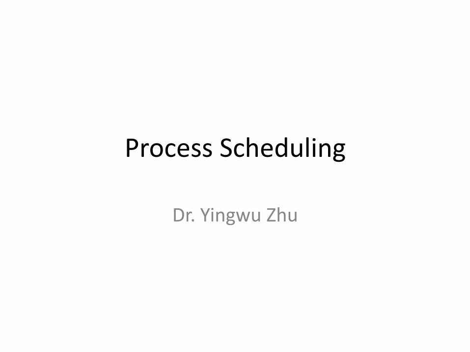
• Most processes exhibit: – Large # of short CPU bursts between I/O requests

– Small # of long CPU bursts between I/O requests

– Interactive process: mostly short CPU bursts

– Compute process: mostly long CPU bursts

Scheduling

• Goal:

– Maximize use of CPU & improve throughput

– Let another process run when the current one is waiting on I/O

• Reality:

– Some processes will use long stretches of CPU time

• Preempt them and let another process run

– More processes may want the CPU: keep them in the ready list

– Perhaps all processes are waiting on I/O: nothing to run!

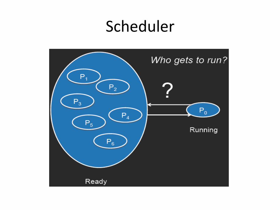
Scheduler

Scheduler

Two components • Scheduling algorithm:

– Policy: Makes the decision of who gets to run

• Dispatcher:

– Mechanism to do the context switch

When does Scheduler Make Decision?

Four events affect the decision: 1. Current process goes from running to waiting state 2. Current process terminates 3. Interrupt causes the scheduler to move a process from

running to ready: – scheduler decides it’s time for someone else to run

4. Current process goes from waiting to ready – I/O (including blocking events, such as semaphores) is complete

• Preemptive scheduler • Cooperative (non-preemptive) scheduler – CPU cannot be taken away

• Run-to-completion scheduler (old batch systems)

Scheduling Algorithm Goals • Be fair (to processes? To users?) • Be efficient: Keep CPU busy … and don’t spend a lot of

time deciding! • Maximize throughput: minimize time users must wait • Minimize response time • Be predictable: jobs should take about the same time

to run when run multiple times • Minimize overhead • Maximize resource use: try to keep devices busy! • Avoid starvation • Enforce priorities • Degrade gracefully: under heavy load

FCFS

• Non-preemptive

• A process with a long CPU burst will hold up other processes

– I/O bound jobs may have completed I/O and are ready to run: poor device utilization

– Poor average response time

Round-Robin Scheduling • Preemptive: Process can not run for longer than a quantum

(time slice) • Performance depends on the time slice

– Long time slice makes this similar to FCFS – Short time slice increases overhead % of context switching

• Advantages – Every process gets an equal share of the CPU – Easy to implement – Easy to compute average response time: f(# processes on list)

• Disadvantage – Giving every process an equal share isn’t necessarily good – Highly interactive processes will get scheduled the same as CPU-

bound processes

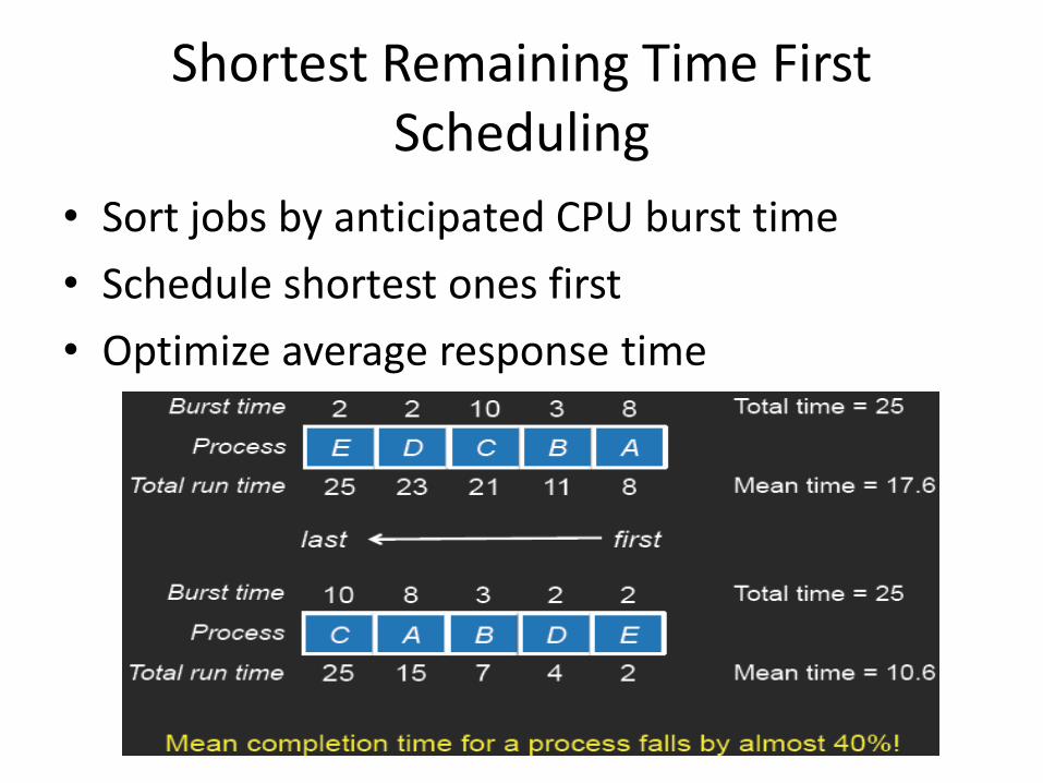
Shortest Remaining Time First Scheduling

• Sort jobs by anticipated CPU burst time

• Schedule shortest ones first

• Optimize average response time

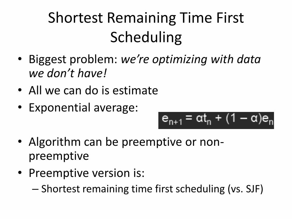
Shortest Remaining Time First Scheduling

• Biggest problem: we’re optimizing with data we don’t have!

• All we can do is estimate

• Exponential average:

• Algorithm can be preemptive or non-preemptive

• Preemptive version is: – Shortest remaining time first scheduling (vs. SJF)

Shortest Remaining Time First Scheduling

• Advantage

– Short-burst jobs run fast

• Disadvantages

– Long-burst (CPU intensive) jobs get a long mean waiting time

– Rely on ability to estimate CPU burst length

Priority Scheduling

• Round Robin assumes all processes are equally important

• Not true – Interactive jobs need high priority for good response – Long non-interactive jobs get worse treatment (get

the CPU less frequently): this goal led us to SRTF – Users may have different status (e.g., administrator)

• Priority scheduling algorithm: – Each process has a priority number assigned to it – Pick the process with the highest priority – Processes with the same priority are scheduled round-

robin

Priority Scheduling

• Priority assignments: – Internal: time limits, memory requirements, I/O:CPU

ratio, … – External: assigned by administrators

• Static & dynamic priorities – Static priority: priority never changes – Dynamic priority: scheduler changes the priority

during execution • Increase priority if it’s I/O bound for better interactive

performance or to increase device utilization • Decrease a priority to let lower-priority processes run • Example: use priorities to drive SJF/SRTF scheduling

Priority Scheduling: dealing with starvation

• Starvation

– Process is blocked indefinitely

– Steady stream of higher-priority processes keeps it from being scheduled

• Dealing with starvation: Process aging

– Gradually increase the priority of a process so that eventually its priority will be high enough so it will be scheduled to run

– Then bring it down again

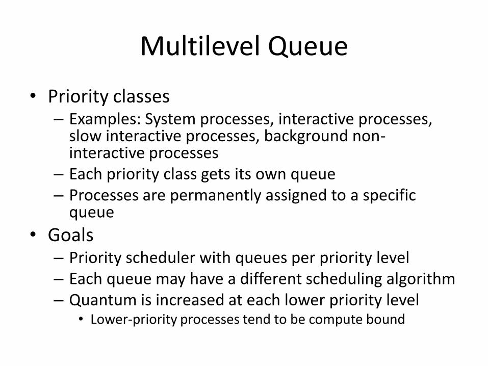
Multilevel Queue

• Priority classes – Examples: System processes, interactive processes,

slow interactive processes, background non-interactive processes

– Each priority class gets its own queue – Processes are permanently assigned to a specific

queue

• Goals – Priority scheduler with queues per priority level – Each queue may have a different scheduling algorithm – Quantum is increased at each lower priority level

• Lower-priority processes tend to be compute bound

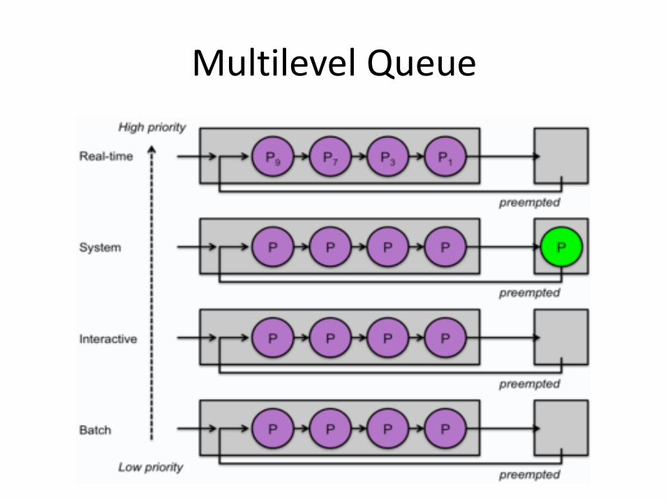
Multilevel Queue

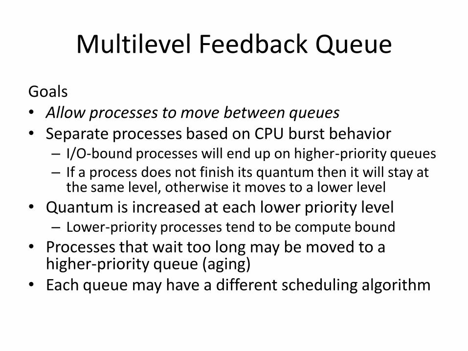
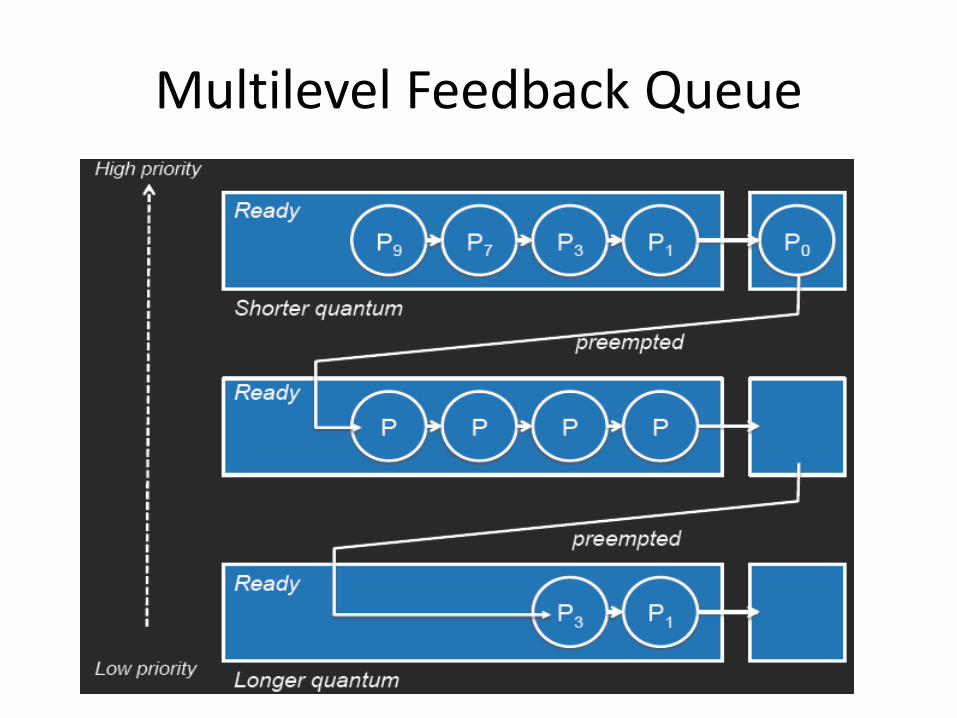
Multilevel Feedback Queue

Goals • Allow processes to move between queues • Separate processes based on CPU burst behavior

– I/O-bound processes will end up on higher-priority queues – If a process does not finish its quantum then it will stay at

the same level, otherwise it moves to a lower level

• Quantum is increased at each lower priority level – Lower-priority processes tend to be compute bound

• Processes that wait too long may be moved to a higher-priority queue (aging)

• Each queue may have a different scheduling algorithm

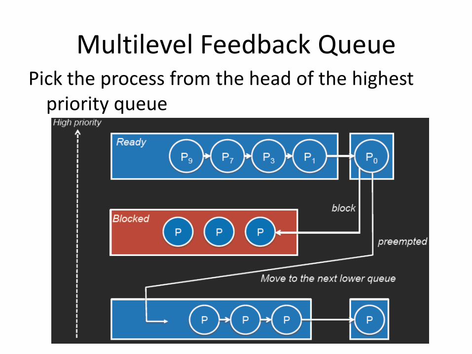
Multilevel Feedback Queue Pick the process from the head of the highest

priority queue

Multilevel Feedback Queue

Multilevel Feedback Queue

• Advantage – Good for separating processes based on CPU burst needs

– Let I/O bound processes run often

– Give CPU-bound processes longer chunks of CPU

– No need to estimate interactivity! (Estimates were often flawed)

• Disadvantages – Priorities get controlled by the system.

• A process is considered important because it uses a lot of I/O

– Processes whose behavior changes may be poorly scheduled

– System can be gamed by scheduling bogus I/O

Symmetric multiprocessor scheduling • SMP: each processor has access to the same memory

and devices. • Processor affinity

– Try to reschedule a process onto the same CPU – Cached memory & TLB lines may be present on the CPU’s

cache

• Types of affinity – Hard : force a process to stay on the same CPU – Soft affinity: best effort, but the process may be

rescheduled on a different CPU • Load balancing: ensure that CPUs are busy • It’s better to run a job on another CPU than wait • If the run queue for a CPU is empty, get a job from another CPU’s

run queue: pull migration • Check load periodically: if not balanced, move jobs. Push migration

Hierarchy of symmetric multiprocessors

• Multiple processors

• Multiple cores

– Shared caches among cores (e.g., Intel i7 cores share L3 cache)

• Hyperthreading

– Presented as two cores to the operating system

– Memory stall: CPU has to wait (e.g., to get data on a cache miss)

– When the issuing logic can no longer schedule instructions from one thread and there are idle functional units in the CPU core, it will try to schedule a suitable instruction from the other thread.

• Good schedulers will know the difference

Linux Scheduler

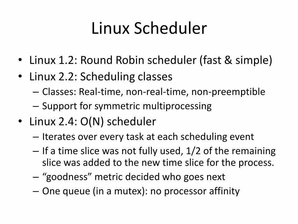
• Linux 1.2: Round Robin scheduler (fast & simple)

• Linux 2.2: Scheduling classes – Classes: Real-time, non-real-time, non-preemptible

– Support for symmetric multiprocessing

• Linux 2.4: O(N) scheduler – Iterates over every task at each scheduling event

– If a time slice was not fully used, 1/2 of the remaining slice was added to the new time slice for the process.

– “goodness” metric decided who goes next

– One queue (in a mutex): no processor affinity

Linux 2.6 O(1) scheduler goals

• Addressed three problems

– Scalability: O(1) instead of O(n) to not suffer under load

– Support processor affinity

– Support preemption

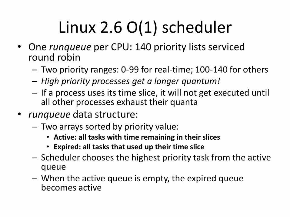
Linux 2.6 O(1) scheduler • One runqueue per CPU: 140 priority lists serviced

round robin – Two priority ranges: 0-99 for real-time; 100-140 for others – High priority processes get a longer quantum! – If a process uses its time slice, it will not get executed until

all other processes exhaust their quanta

• runqueue data structure: – Two arrays sorted by priority value:

• Active: all tasks with time remaining in their slices • Expired: all tasks that used up their time slice

– Scheduler chooses the highest priority task from the active queue

– When the active queue is empty, the expired queue becomes active

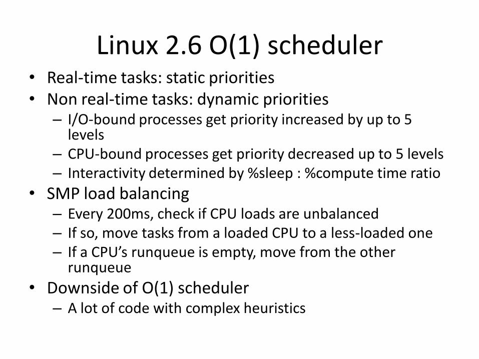
Linux 2.6 O(1) scheduler • Real-time tasks: static priorities • Non real-time tasks: dynamic priorities

– I/O-bound processes get priority increased by up to 5 levels

– CPU-bound processes get priority decreased up to 5 levels – Interactivity determined by %sleep : %compute time ratio

• SMP load balancing – Every 200ms, check if CPU loads are unbalanced – If so, move tasks from a loaded CPU to a less-loaded one – If a CPU’s runqueue is empty, move from the other

runqueue

• Downside of O(1) scheduler – A lot of code with complex heuristics

Linux Completely Fair Scheduler

• Latest scheduler (introduced in 2.6.23)

• Goal: give a “fair” amount of CPU time to tasks

• Keep track of time given to a task (“virtual runtime”)

– Also use “sleeper fairness”: tasks get a “fair” share of the CPU even if they sleep from time to time

• Priorities

– Used as a decay factor for the time a task is permitted to execute

– Allowable time decreases for low priority tasks

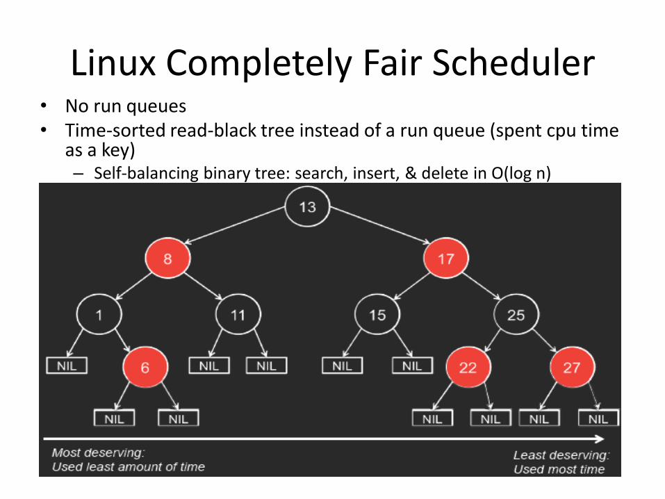
Linux Completely Fair Scheduler • No run queues • Time-sorted read-black tree instead of a run queue (spent cpu time

as a key) – Self-balancing binary tree: search, insert, & delete in O(log n)

CFS: picking a process

• Scheduling decision: – Pick the leftmost task

• When a process is done: – Add execution time to the per-task run time count

– Insert the task back in the queue

• Heuristic: decay factors – Determine how long a task can execute

– Higher priority tasks have lower factors of decay.

– Avoids having run queues per priority level

Acknowledgements

• Some of slides are adapted from Paul Krzyzanowski