PROCESS PLANNING METHOD FOR EXPOSURE CONTROLLED PROJECTION

LITHOGRAPHY

Amit S. Jariwala, Harrison Jones, Abhishek Kwatra, David W. Rosen*

George W. Woodruff School of Mechanical Engineering

Georgia Institute of Technology

Atlanta, Georgia, 30332

*Corresponding author. Tel.: +1 404 894 9668 Email: david.rosen@me.gatech.edu

Abstract:

An Exposure Controlled Projection Lithography (ECPL) process with the ability to cure

lens shaped structures on transparent substrates is presented. This process can be used to create

microlenses and micro fluidic channels on flat or curved substrates. Incident radiation, patterned

by a dynamic mask, passes through a transparent substrate to cure photopolymer resin that grows

progressively from the substrate surface. A resin response model which incorporates the effects

of oxygen inhibition during photopolymerization is used to formulate a process planning method

for ECPL. This process planning method is validated for fabricating lens shaped structure on flat

transparent substrates using the ECPL system.

1. Introduction

Exposure Controlled Projection Lithography (ECPL) is an additive manufacturing

process used to build physical components out of a photopolymer resin. In conventional

Stereolithography (“SLA”), a solid object is built layer by layer by exposing successive thin

layers of photopolymer resin to a scanned laser beam. Recently researchers including Bertsch et

al. [1], Chatwin [2], Monneret et al. [3], Sun et al. [4] and Limaye and Rosen [5] have

demonstrated the use of a dynamic mask such as Texas Instruments’ Digital Micromirror Device

(DMD™) in conventional SLA instead of using a scanned laser beam. Some commercially

available machines, such as the Perfactory® range of machines from EnvisonTec, Germany, also

use one or more DMD™ chips to pattern the light in a conventional layer-by-layer SLA process

[6]. Unlike these processes, ECPL utilizes the dynamic mask such that the irradiation from the

DMD™ chip passes through a transparent substrate into a resin vat, and it uses careful control of

the light intensity profile to define the vertical shape of the object being fabricated instead of the

layer-by-layer approach used in conventional SLA processes. By using a gray-scale image, or

alternatively a series of binary bitmap images, both the shape and the intensity profile of the

irradiation can be controlled simultaneously; this in turn provides control over the photochemical

polymerization reaction in three dimensions. Similar techniques have been investigated by other

researchers, in various forms. Erdmann et al. [7] have used mask projection stereolithography

through transparent substrates for the fabrication of simple micro-lens arrays, and Mizukami et

al. [8] have proposed the use of laser beam scanning through transparent substrates to cure

photopolymers for the manufacture of micro-electrophoretic chips. However, to date there is a

substantial lack of knowledge with regard to controlling the process in order to achieve the

desired accuracy and precision over the final cured parts.

95

Limaye and Rosen [5] recently proposed a process planning method to control the lateral

dimensions of the cured part in a conventional mask-based stereolithography process (then

referred to as Mask Projection micro-SLA, or MPµSLA), although the proposed process plan

was not intended to precisely control the curing front in the vertical dimension. Jariwala et al. [9]

later proposed an elementary process planning method for controlling the cured profile of a thin

film cured on a transparent substrate. The process planning method incorporated both a ray

tracing model and a basic photopolymerization kinetic model to estimate the required fabrication

parameters. Since the process plan was based on a simple polymerization model, the results

showed significant deviations in all dimensions. It was hypothesized that the inaccuracies were

largely the result of oxygen diffusion and inhibition during the polymerization process. Jariwala

et al. [10] subsequently developed a photopolymerization model based on differential equations

to model and simulate the effects of oxygen inhibition during polymerization. Although

modeling the oxygen inhibition process provided results that more closely matched the observed

experimental trends, the model was found inadequate to completely predict the exact shape of

the cured part.

In this paper, the chemical reactions occurring during photopolymerization were modeled

with revised rate constants. Experiments suggest that the finite element models with revised rate

constants can better predict the shape of the cured part. These models were simulated in

COMSOL® software package to generate empirical models, which were then used to formulate

the process plan. This paper demonstrates a unique process planning approach which involves

using iterative chemical simulations to optimize the process inputs required to cure a desired

shape from ECPL system.

2. ECPL System

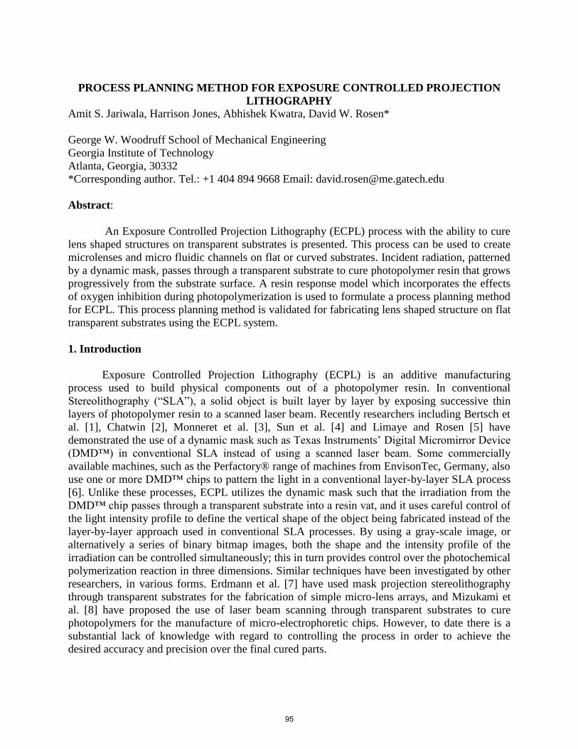
The block diagram of the

ECPL process is illustrated in

Figure 1. A UV light source is

used with a 365nm filter and the

light is passed onto the beam

conditioning system. The

objective of this beam

conditioning system is to

homogenize the light output

from the light source and project

it onto the Digital Micromirror Device (DMD™), which is used as a dynamic mask to project

grayscale images. The projection system reduces the size of the image projected on the DMD™

and focuses in into the resin chamber. The resin chamber consists of a standard glass microscope

slide which acts as a base, an identical glass slide which serves as a top, and spacers of various

thicknesses depending on the dimensions of the object to be formed; the liquid photopolymer is

placed inside this chamber.

Grayscale images are formed on the DMD™ using the computer and projected from the

DMD™ into the resin chamber. The regions of the liquid photopolymer resin which receive the

irradiation cross-link and are converted into solid polymer, with a vertical profile that roughly

matches the intensity profile of the incident light. The uncured monomer is then washed off the

cured part in the “developing” process, and the final cured part is obtained on the glass slide. The

details of all these modules are explained in Jariwala et al [11]. The discussions in this paper

Fig. 1 Block diagram of the ECPL process

96

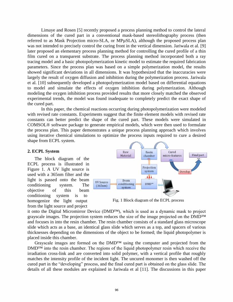
primarily relate to the chemical reactions

occurring within the resin chamber, which

consists of two glass slide stuck closely together

with a spacer of known thickness placed along

two edges as shown schematically in Figure 2.

The resin is loaded between this sandwich

structure of glass slides and is held by capillary

force. The base glass slide acts as the substrate

upon which the film is cured.

3.1 Analytical Modeling – Irradiance Model

The ECPL system is analytically modeled

in two phases – Irradiance Model and

Photopolymerization Model. The irradiance

model models the irradiance received by the resin

in terms of the process parameters and is

presented in detail in Jariwala et al. [12]. The

irradiance distribution on the resin depends upon

the power distribution across the light beam

incident on the bitmap and upon the optical

aberrations caused by the imaging lens. This

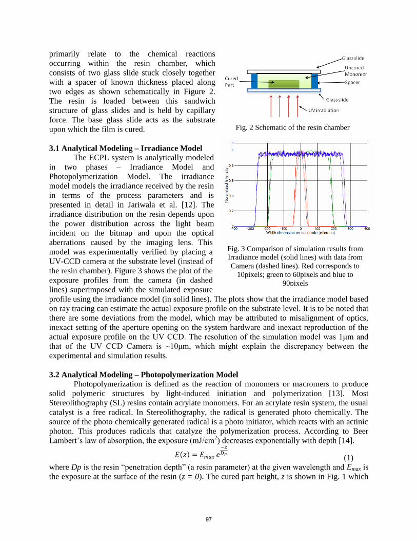
model was experimentally verified by placing a

UV-CCD camera at the substrate level (instead of

the resin chamber). Figure 3 shows the plot of the

exposure profiles from the camera (in dashed

lines) superimposed with the simulated exposure

profile using the irradiance model (in solid lines). The plots show that the irradiance model based

on ray tracing can estimate the actual exposure profile on the substrate level. It is to be noted that

there are some deviations from the model, which may be attributed to misalignment of optics,

inexact setting of the aperture opening on the system hardware and inexact reproduction of the

actual exposure profile on the UV CCD. The resolution of the simulation model was 1μm and

that of the UV CCD Camera is ~10μm, which might explain the discrepancy between the

experimental and simulation results.

3.2 Analytical Modeling – Photopolymerization Model

Photopolymerization is defined as the reaction of monomers or macromers to produce

solid polymeric structures by light-induced initiation and polymerization [13]. Most

Stereolithography (SL) resins contain acrylate monomers. For an acrylate resin system, the usual

catalyst is a free radical. In Stereolithography, the radical is generated photo chemically. The

source of the photo chemically generated radical is a photo initiator, which reacts with an actinic

photon. This produces radicals that catalyze the polymerization process. According to Beer

Lambert’s law of absorption, the exposure (mJ/cm2) decreases exponentially with depth [14].

(1)

where Dp is the resin “penetration depth” (a resin parameter) at the given wavelength and Emax is

the exposure at the surface of the resin (z = 0). The cured part height, z is shown in Fig. 1 which

𝐸 𝑧 = 𝐸𝑚𝑎𝑥 𝑒−𝑧𝐷𝑃

Fig. 2 Schematic of the resin chamber

Fig. 3 Comparison of simulation results from

Irradiance model (solid lines) with data from

Camera (dashed lines). Red corresponds to

10pixels; green to 60pixels and blue to

90pixels

97

shows the schematic of the polymerization process studied in this paper. Based on experimental

observations, this model was modified in [3, 4] as follows:

z 𝐷 (

−

) (2)

The parameters Ec, DpL and DpS are usually fit to experimental data at a specific resin

composition and cure intensity. In practice, polymerization does not proceed beyond a limited

depth where the exposure falls below a threshold value, Ec. This is primarily due to oxygen

inhibition, which imposes a minimal threshold to start polymerization. This exposure threshold

model is an oversimplification of the SL process. It directly connects the exposure to the resin

and the final solid part shape. It ignores many important intermediate steps. Its ability to predict

the three dimensional cured part outline is challenged especially when part resolution is in

demand, since it is a one-dimensional model. This shortcoming can be observed by using the

empirical polymerization model with the irradiance model.

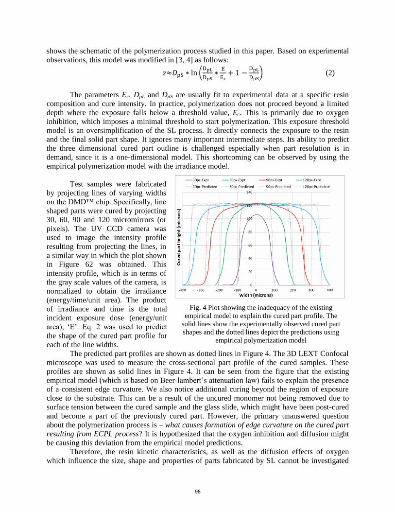
Test samples were fabricated

by projecting lines of varying widths

on the DMD™ chip. Specifically, line

shaped parts were cured by projecting

30, 60, 90 and 120 micromirrors (or

pixels). The UV CCD camera was

used to image the intensity profile

resulting from projecting the lines, in

a similar way in which the plot shown

in Figure 62 was obtained. This

intensity profile, which is in terms of

the gray scale values of the camera, is

normalized to obtain the irradiance

(energy/time/unit area). The product

of irradiance and time is the total

incident exposure dose (energy/unit

area), ‘E’. Eq. 2 was used to predict

the shape of the cured part profile for

each of the line widths.

The predicted part profiles are shown as dotted lines in Figure 4. The 3D LEXT Confocal

microscope was used to measure the cross-sectional part profile of the cured samples. These

profiles are shown as solid lines in Figure 4. It can be seen from the figure that the existing

empirical model (which is based on Beer-lambert’s attenuation law) fails to explain the presence

of a consistent edge curvature. We also notice additional curing beyond the region of exposure

close to the substrate. This can be a result of the uncured monomer not being removed due to

surface tension between the cured sample and the glass slide, which might have been post-cured

and become a part of the previously cured part. However, the primary unanswered question

about the polymerization process is – what causes formation of edge curvature on the cured part

resulting from ECPL process? It is hypothesized that the oxygen inhibition and diffusion might

be causing this deviation from the empirical model predictions.

Therefore, the resin kinetic characteristics, as well as the diffusion effects of oxygen

which influence the size, shape and properties of parts fabricated by SL cannot be investigated

Fig. 4 Plot showing the inadequacy of the existing

empirical model to explain the cured part profile. The

solid lines show the experimentally observed cured part

shapes and the dotted lines depict the predictions using

empirical polymerization model

98

by using this empirical model. Available chemical models presented in literature only focus on

predicting part height and none of them present any approach to predict the shape of the cured

profile. We present a unique two dimensional model which can be used to predict part height as

well as the shape of the overall cured profile.

The kinetic model for multifunctional acrylate photopolymerization presented here, is

based on a set of ordinary differential equations (ODE). The final results show that the kinetic

ODE model, based on the critical conversion value, incorporates the impact of process

parameters such as initiator concentration, light intensity, oxygen diffusion and exposure time on

the final part profile of the object. In addition, the part height predictions from the ODE model

are comparable to experiments and the predictions from the modified Ec–Dp model.

4. Polymerization Model

4.1 Photopolymerization Kinetics

Recently, Boddapati et al. [15] developed a model to predict the gel time for

multifunctional acrylates using a kinetics model. This model incorporated the effects of oxygen

inhibition and diffusion in one dimension, which was parallel to the direction of UV irradiation.

The rate constants were optimized to fit the experimental data. There were four unique rate

constants in the kinetic model, with the diffusivity of oxygen in the photopolymer resin. For ease

of reference, the kinetic model is presented as follows. The concentrations of photoinitiator [In],

radicals [𝑅 ∙], unreacted double bonds [DB], and oxygen [O2] were modeled in the kinetic

model. The reactions considered by them were as follows [15]. When the photopolymer resin

receives light energy, the photoinitiator absorbs it and decomposes into two radicals with first

order rate constant of, 𝐾𝑑.

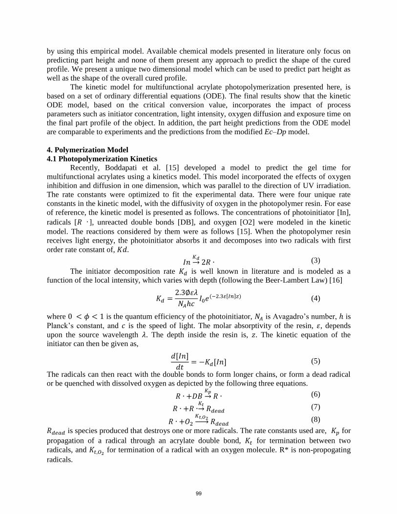
→ 𝑅 (3)

The initiator decomposition rate 𝐾 is well known in literature and is modeled as a

function of the local intensity, which varies with depth (following the Beer-Lambert Law) [16]

𝐾

𝑒

[ ] (4)

where is the quantum efficiency of the photoinitiator, is Avagadro’s number, is

Planck’s constant, and is the speed of light. The molar absorptivity of the resin, , depends

upon the source wavelength . The depth inside the resin is, 𝑧. The kinetic equation of the

initiator can then be given as,

𝑑[ ]

𝑑 −𝐾 [ ] (5)

The radicals can then react with the double bonds to form longer chains, or form a dead radical

or be quenched with dissolved oxygen as depicted by the following three equations.

𝑅 𝐷 → 𝑅 (6)

𝑅 𝑅 → 𝑅 (7)

𝑅

→ 𝑅 (8)

𝑅 is species produced that destroys one or more radicals. The rate constants used are, 𝐾 for

propagation of a radical through an acrylate double bond, 𝐾 for termination between two

radicals, and 𝐾 for termination of a radical with an oxygen molecule. R* is non-propogating

radicals.

99

The overall rate of initiator decomposition, 𝑅 , is modeled by multiplying the rate

constant 𝐾 by the initiator concentration [ ]

𝑅 𝐾 [ ] (9)

The kinetic equations for the double bond [𝐷 ], live radicals [𝑅 ] and oxygen [ ] can

be given as follows:

𝑑[𝑅 ]

𝑑 𝑧 [ ] − [𝑅 ] −

[𝑅 ][ ] (10)

𝑑[𝐷 ]

𝑑 − [𝑅 ][𝐷 ] (11)

[ ]

−

[𝑅 ][ ] 𝐷

[ ]

𝑧 (12)

The effect of oxygen inhibition and diffusion was explicitly modeled in Eq. 12. Due to

the high diffusivity of dissolved oxygen in the photopolymer resin, it was assumed that the

oxygen would primarily diffuse from uncured top layers of the sample chamber down to the

curing front, competing with double bonds for radicals and significantly slowing down the rate at

which the double bonds are converted, thus increasing the gel time. This equation was modified

to account for oxygen diffusion in two dimensions as shown in Eq. 13.

[ ]

−

[𝑅 ][ ] 𝐷

[ ]

𝑥 𝐷

[ ]

𝑧

(13)

The researchers estimated the rate constants, 𝐾 𝐾 𝐾 by fitting the simulation

results with the experimental data from FTIR. They had suggested that the individual rate

constants are not unique and may vary. Since, the FTIR experiments were conducted at 100

times the intensity of the light used in the ECPL system, it is possible that the effect of oxygen

inhibition and diffusion was not adequately captured using the presented rate constants. Hence,

these constants were varied to suit the ECPL experimental conditions. The physical parameters,

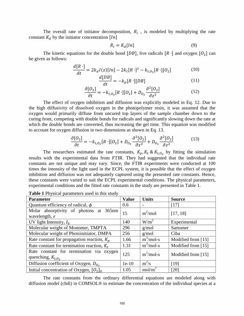
experimental conditions and the fitted rate constants in the study are presented in Table 1.

Table 1 Physical parameters used in this study

Parameter Value Units Source

Quantum efficiency of radical, 0.6 - [17]

Molar absorptivity of photons at 365nm

wavelength, 15 m

2/mol [17, 18]

UV light Intensity, 140 W/m2 Experimental

Molecular weight of Monomer, TMPTA 296 g/mol Sartomer

Molecular weight of Photoinitiator, DMPA 256 g/mol Ciba

Rate constant for propagation reaction, 𝐾 1.66 m3/mol-s Modified from [15]

Rate constant for termination reaction, 𝐾 1.31 m3/mol-s Modified from [15]

Rate constant for termination via oxygen

quenching, 𝐾

125 m3/mol-s Modified from [15]

Diffusion coefficient of Oxygen, 𝐷 1e-10 m

2/s [19]

Initial concentration of Oxygen, [ ] 1.05 mol/m3 [20]

The rate constants from the ordinary differential equations are modeled along with

diffusion model (chdi) in COMSOL® to estimate the concentration of the individual species at a

100

given time at a specified location within the resin chamber. The concentration of reactants,

especially the monomer concentration [M], during the curing process, can be used to estimate the

thickness and profile of the cured part.

Carothers and Flory described a gel as an infinitely large molecule that is insoluble [21,

22, and 23]. Flory used this definition to estimate the degree of cure necessary for the onset of

gelation based on the functionality of the reacting monomers [23]. Once the resin starts to gel,

the viscosity of the solution increases sharply, and the cure undergoes a rapid transition from a

liquid state to a solid state [24]. The degree of cure or the monomer conversion is computed

using the following formula. The monomer concentration after polymerization is represented as

[M] and the initial monomer concentration is represented as [M0].

𝑒 [ ] [ ]

[ ] (14)

The shape of the cured part can then be estimated by tracking the coordinates within the

sample where the conversion has reached the critical conversion limit. Using the rate constants

shown in table 1, a conversion cut-off value of 12%was determined by fitting to the experimental

data for TMPTA with oxygen in [16].

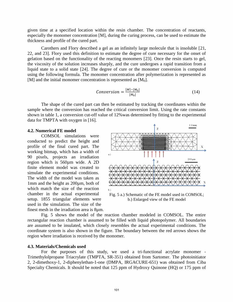
4.2. Numerical FE model

COMSOL simulations were

conducted to predict the height and

profile of the final cured part. The

working bitmap, which has a width of

90 pixels, projects an irradiation

region which is 560µm wide. A 2D

finite element model was created to

simulate the experimental conditions.

The width of the model was taken as

1mm and the height as 200µm, both of

which match the size of the reaction

chamber in the actual experimental

setup. 1855 triangular elements were

used in the simulation. The size of the

finest mesh in the irradiation area is 8µm.

Fig. 5 shows the model of the reaction chamber modeled in COMSOL. The entire

rectangular reaction chamber is assumed to be filled with liquid photopolymer. All boundaries

are assumed to be insulated, which closely resembles the actual experimental conditions. The

coordinate system is also shown in the figure. The boundary between the red arrows shows the

region where irradiation is received by the monomer.

4.3. Materials/Chemicals used

For the purposes of this study, we used a tri-functional acrylate monomer -

Trimethylolpropane Triacrylate (TMPTA, SR-351) obtained from Sartomer. The photoinitiator

2, 2-dimethoxy-1, 2-diphenylethan-1-one (DMPA, IRGACURE-651) was obtained from Ciba

Specialty Chemicals. It should be noted that 125 ppm of Hydroxy Quinone (HQ) or 175 ppm of

Fig. 5 a.) Schematic of the FE model used in COMSOL;

b.) Enlarged view of the FE model

101

Hydroquinone Monomethyl Ether (MEHQ) are included in the monomer formulation of TMPTA

to inhibit polymerization from hydroxy radicals while in storage, and the inhibitor was not

removed from the experiments, unless specifically noted. The above ppm concentrations are

equivalent to the molar concentration of oxygen in the sample, but the exact amount of inhibitor

in the monomer at the time of use can vary, and it has been shown that these inhibitors do not

impede the photopolymerization as strongly as Oxygen does. All experiments were neat

solutions (containing no additional solvent) of TMPTA prepared at near constant initiator

concentration of 20% w/w for TMPTA.

4.4. Experimental Validation

The resin in the reaction chamber was cured by the UV irradiation patterned by the bitmaps

on DMD™. Experiments were conducted on the ECPL system. The polymerized parts were

cured on a glass slide. After curing, the glass slide is removed from the resin chamber and

additional uncured resin is removed using an air duster. A 3D laser LEXT confocal microscope

was used to measure the cured part profile using the glass slide as the reference.

T

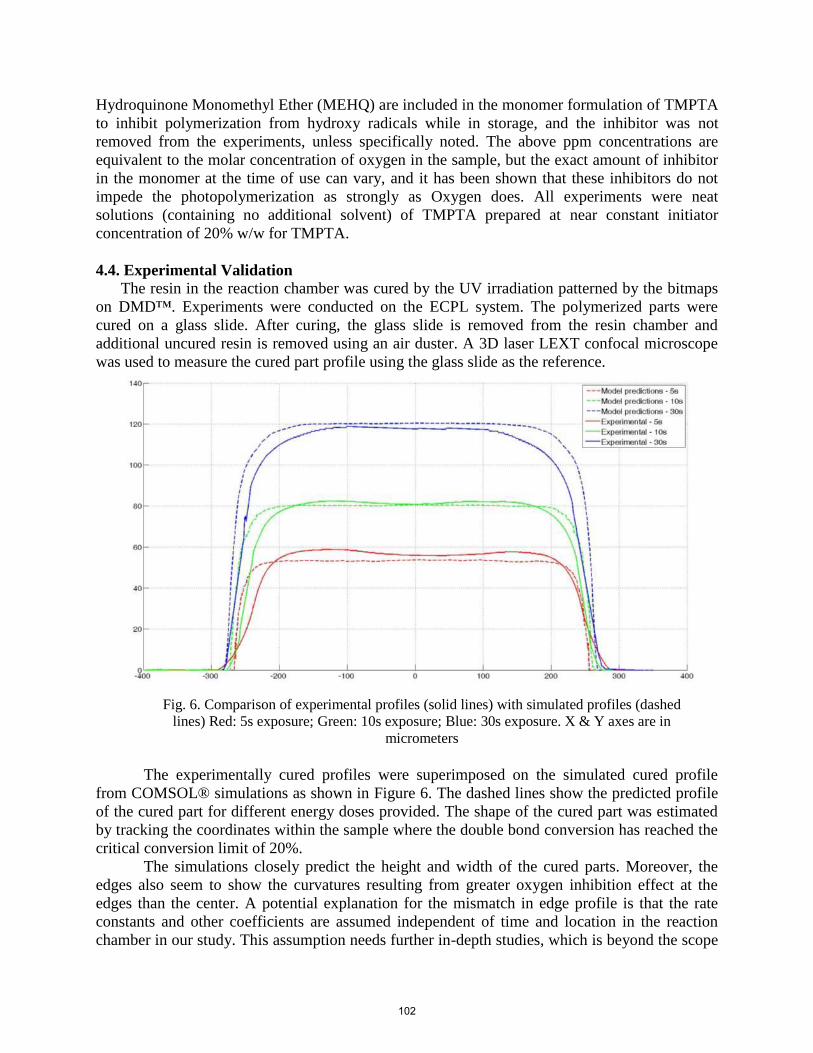
The experimentally cured profiles were superimposed on the simulated cured profile

from COMSOL® simulations as shown in Figure 6. The dashed lines show the predicted profile

of the cured part for different energy doses provided. The shape of the cured part was estimated

by tracking the coordinates within the sample where the double bond conversion has reached the

critical conversion limit of 20%.

The simulations closely predict the height and width of the cured parts. Moreover, the

edges also seem to show the curvatures resulting from greater oxygen inhibition effect at the

edges than the center. A potential explanation for the mismatch in edge profile is that the rate

constants and other coefficients are assumed independent of time and location in the reaction

chamber in our study. This assumption needs further in-depth studies, which is beyond the scope

Fig. 6. Comparison of experimental profiles (solid lines) with simulated profiles (dashed

lines) Red: 5s exposure; Green: 10s exposure; Blue: 30s exposure. X & Y axes are in

micrometers

102

of this paper. A second potential explanation is shrinkage. Shrinkage during resin cure causes

reduction in feature dimensions, but it also causes residual stresses, which can lead to distortions

in part shapes. Investigation of shrinkage can be a future scope of work, which may be

conducted in order to improve the predictability of the model. Despite these limitations, the

COMSOL® simulations successfully demonstrate the generation of curved edges for the cured

parts. This effect of oxygen inhibition was not considered using the empirical 𝐸 − 𝐷 model. It

can only predict that the final cured shape will be the same height and will fail to show the edge

curvatures. Hence, the 𝐸 − 𝐷 model, in its original form, cannot be used to predict the shape of

the cured part.

5. Process Plan Formulation

The existing process planning methods for ECPL based systems are discussed in

literature as presented in Jariwala et al. [9, 12] & Zhao [25]. Through detailed experimentation

and error analysis, it was found that the process planning method had several drawbacks. The

researchers did not have access to effective metrology tools and hence the experimental

validation of their proposed planning methods was not adequate. Moreover, the process-planning

algorithm assumed that the complex process of photopolymerization could be assumed as a

simple exponential function of exposure (based on the Beer-Lambert law for attenuation).

Although the incident exposure (required to cure the photopolymer) can be considered additive,

the effect of curing is not necessarily additive in nature. As shown in Section 3.2 and Section 4,

the polymerization process is highly coupled and the shape and dimensions of the final cured

product depends on the entire exposure pattern and sequence of exposure.

The process-planning problem, as derived from existing literature was split into two parts

i.) Conversion of desired product geometry/shape in to required exposure

ii.) Estimation of required exposure in to process inputs

a. Estimation of time of exposure for each micromirror

b. Clustering of micromirrors into bitmaps with common times of exposure

The problem for process planning is to estimate the accurate bitmaps and corresponding

exposure time required to cure the desired part shape. This problem can be simplified to a

significant extent for the ECPL system studied in this research. The ECPL system can only

fabricate structures with monotonically decreasing part geometries, i.e. it is reasonable to assume

that the size of the total exposed region should gradually decrease (or remain constant) as more

and more height of the cured part is formed. This helps in greatly constraining the optimization

problem proposed in the revised hypothesis. Moreover, since the research objective was to

fabricate lens like axi-symmetric shapes, the optimization problem can be kept limited to curing

two-dimensional axi-symmetric profiles at the center of the substrate.

The overall problem presented by the research question can be simplified as generating

the process inputs (a line of clustered micromirrors with corresponding times of exposure)

necessary to cure the half-sectional profile of the desired part geometry. Once the line of

clustered micromirrors is estimated, the bitmap can be generated by ‘rotating’ the micromirrors

along 360° to generate the bitmap. Hence, the process inputs can be listed as follows and

illustrated in Figure 7.

103

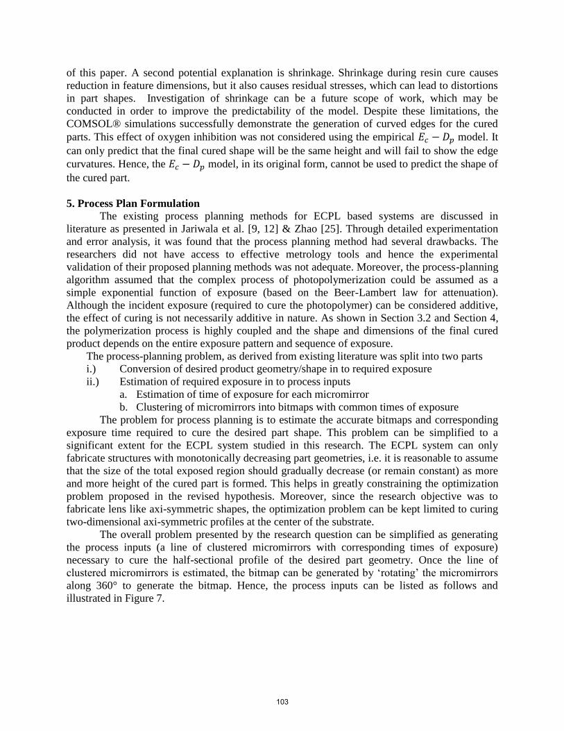
– Bitmap used to cure the ith

layer, such that is the number of

micromirrors offset from the center of the

part to be cured and 𝑅 is the total number

of micromirrors from the center of the part

to be cured.

– Calculated exposure time for

ith

bitmap

It is to be noted that the first

“layer” would be cured on the substrate

and hence will not be affected by the

previous history of exposure. Hence,

estimation of the first group of process

inputs (bitmaps and corresponding

exposure time) can be made using a pre-calculated material database model based. The process

inputs to cure the subsequent “layers” can be estimated using iterative simulations of the

chemical kinetic model. Hence, the process planning method can be simplified in form of two-

step process as follows:

1. Estimate the first set of process input (bitmap#1 and exposure time) by optimizing

the cured part shape using a pre-calculated material database model.

2. Estimate the subsequent process inputs by optimizing the cured part shape using

actual simulations of the chemical kinetic model.

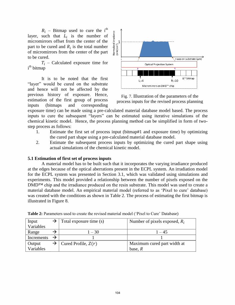
5.1 Estimation of first set of process inputs

A material model has to be built such that it incorporates the varying irradiance produced

at the edges because of the optical aberrations present in the ECPL system. An irradiation model

for the ECPL system was presented in Section 3.1, which was validated using simulations and

experiments. This model provided a relationship between the number of pixels exposed on the

DMD™ chip and the irradiance produced on the resin substrate. This model was used to create a

material database model. An empirical material model (referred to as ‘Pixel to cure’ database)

was created with the conditions as shown in Table 2. The process of estimating the first bitmap is

illustrated in Figure 8.

Table 2: Parameters used to create the revised material model (‘Pixel to Cure’ Database)

Input

Variables

Total exposure time (s) Number of pixels exposed, 𝑅

Range 1 – 30 1 – 45

Increments 1 1

Output

Variables

Cured Profile, Maximum cured part width at

base, 𝑅

Fig. 7. Illustration of the parameters of the

process inputs for the revised process planning

method

104

With reference to Figure 8,

the first bitmap and exposure time

were estimated by optimizing the

cured part edge. It is to be noted

that the primary function of the

first bitmap is not to cure the

entire part geometry, but to cure

the base and the corresponding

edge of the desired part. Hence,

the optimization problem is not to

be assumed to optimize the entire

cured part geometry. Rather, the

objective function of the

optimization problem is changed

based on the resulting cured part

height. This explanation can be

mathematically explained as

follows.

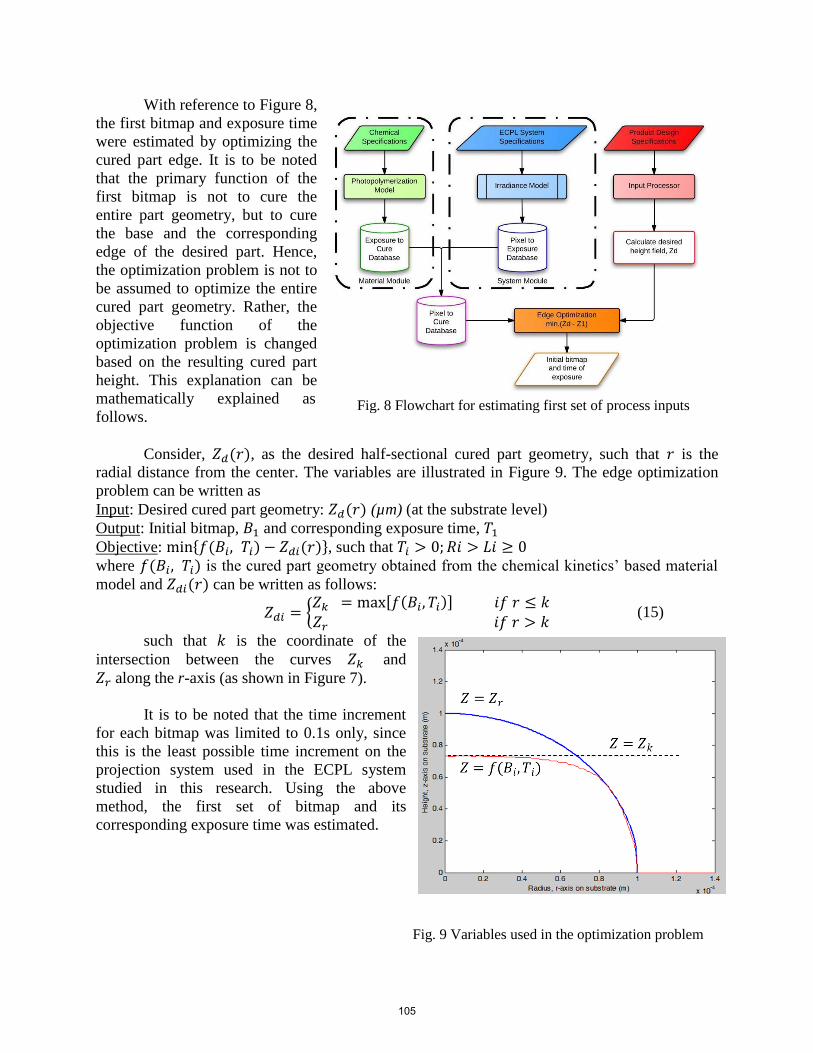
Consider, , as the desired half-sectional cured part geometry, such that is the

radial distance from the center. The variables are illustrated in Figure 9. The edge optimization

problem can be written as

Input: Desired cured part geometry: (µm) (at the substrate level)

Output: Initial bitmap, and corresponding exposure time,

Objective: { − }, such that 𝑅

where is the cured part geometry obtained from the chemical kinetics’ based material

model and can be written as follows:

{ [ ]

(15)

such that is the coordinate of the

intersection between the curves and

along the r-axis (as shown in Figure 7).

It is to be noted that the time increment

for each bitmap was limited to 0.1s only, since

this is the least possible time increment on the

projection system used in the ECPL system

studied in this research. Using the above

method, the first set of bitmap and its

corresponding exposure time was estimated.

Fig. 9 Variables used in the optimization problem

Fig. 8 Flowchart for estimating first set of process inputs

105

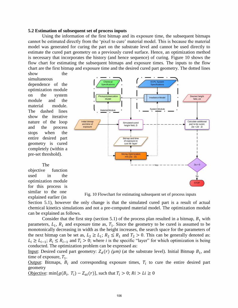
5.2 Estimation of subsequent set of process inputs

Using the information of the first bitmap and its exposure time, the subsequent bitmaps

cannot be estimated directly from the ‘pixel to cure’ material model. This is because the material

model was generated for curing the part on the substrate level and cannot be used directly to

estimate the cured part geometry on a previously cured surface. Hence, an optimization method

is necessary that incorporates the history (and hence sequence) of curing. Figure 10 shows the

flow chart for estimating the subsequent bitmaps and exposure times. The inputs to the flow

chart are the first bitmap and exposure time and the desired cured part geometry. The dotted lines

show the

simultaneous

dependence of the

optimization module

on the system

module and the

material module.

The dashed lines

show the iterative

nature of the loop

and the process

stops when the

entire desired part

geometry is cured

completely (within a

pre-set threshold).

The

objective function

used in the

optimization module

for this process is

similar to the one

explained earlier (in

Section 5.1), however the only change is that the simulated cured part is a result of actual

chemical kinetics simulations and not a pre-computed material model. The optimization module

can be explained as follows.

Consider that the first step (section 5.1) of the process plan resulted in a bitmap, with

parameters, , 𝑅 and exposure time as, . Since the geometry to be cured is assumed to be

monotonically decreasing in width as the height increases, the search space for the parameters of

the next bitmap can be set as, ; 𝑅 𝑅 and . This can be generally denoted as:

; 𝑅 𝑅 and ; where i is the specific “layer” for which optimization is being

conducted. The optimization problem can be expressed as:

Input: Desired cured part geometry: (µm) (at the substrate level). Initial Bitmap , and

time of exposure, .

Output: Bitmaps, and corresponding exposure times, to cure the entire desired part

geometry

Objective: { − }, such that ; 𝑅

Fig. 10 Flowchart for estimating subsequent set of process inputs

106

where is the cured part geometry obtained from the chemical kinetics’ based

simulations and can be written as follows:

{ [ ] − 𝑚 𝑚

(16)

such that 𝑚 is the coordinate of the intersection between the curves and along the

r-axis (similar to ‘k’, as shown in Figure 9). is the additional part to be cured and calculated

as follows:

− (17)

Both the first and second stages of the process plan were coded using Matlab and several

example cases were tested. The following sections present the validation to the revised

hypothesis using the test cases, both through simulations and experiments.

8. Results and Discussions

In order to validate the process planning method, experiments were conducted on the

ECPL system. Matlab scripts were written to encode the revised process planning algorithm. The

bitmaps resulting from the process planning method were projected on the DMD™ in the ECPL

system for their corresponding times of exposure. The cured samples were then washed, post-

cured and measured using the LEXT 3D confocal microscope. The following sub-sections

present the results of each sample.

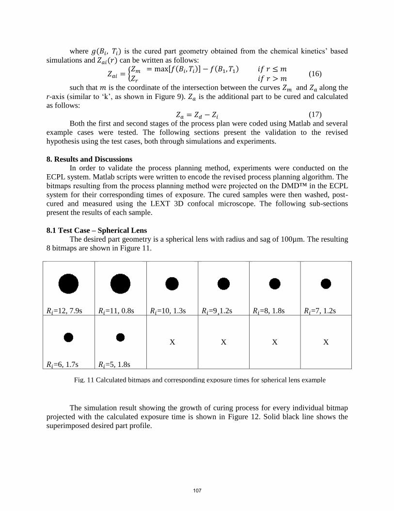
8.1 Test Case – Spherical Lens

The desired part geometry is a spherical lens with radius and sag of 100µm. The resulting

8 bitmaps are shown in Figure 11.

𝑅 =12, 7.9s

𝑅 =11, 0.8s

𝑅 =10, 1.3s

𝑅 =9¸1.2s

𝑅 =8, 1.8s

𝑅 =7, 1.2s

𝑅 =6, 1.7s

𝑅 =5, 1.8s

X X X X

The simulation result showing the growth of curing process for every individual bitmap

projected with the calculated exposure time is shown in Figure 12. Solid black line shows the

superimposed desired part profile.

Fig. 11 Calculated bitmaps and corresponding exposure times for spherical lens example

107

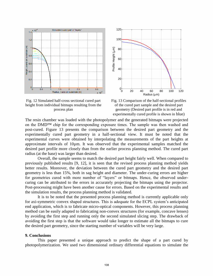
The resin chamber was loaded with the photopolymer and the generated bitmaps were projected

on the DMD™ chip for the corresponding exposure times. The sample was then washed and

post-cured. Figure 13 presents the comparison between the desired part geometry and the

experimentally cured part geometry in a half-sectional view. It must be noted that the

experimental curves were obtained by interpolating the measurements of the part heights at

approximate intervals of 10µm. It was observed that the experimental samples matched the

desired part profile more closely than from the earlier process planning method. The cured part

radius (at the base) was larger than desired.

Overall, the sample seems to match the desired part height fairly well. When compared to

previously published results [9, 12], it is seen that the revised process planning method yields

better results. Moreover, the deviation between the cured part geometry and the desired part

geometry is less than 15%, both in sag height and diameter. The under-curing errors are higher

for geometries cured with more number of “layers” or bitmaps. Hence, the observed under-

curing can be attributed to the errors in accurately projecting the bitmaps using the projector.

Post-processing might have been another cause for errors. Based on the experimental results and

the simulation results, the process planning method is validated.

It is to be noted that the presented process planning method is currently applicable only

for axi-symmetric convex shaped structures. This is adequate for the ECPL system’s anticipated

end application, which is to fabricate micro-optical components. However, this process planning

method can be easily adapted to fabricating non-convex structures (for example, concave lenses)

by avoiding the first step and running only the second simulated slicing step. The drawback of

avoiding the first step is that the software would take longer to estimate all the bitmaps to cure

the desired part geometry, since the starting number of variables will be very large.

9. Conclusions

This paper presented a unique approach to predict the shape of a part cured by

photopolymerization. We used two dimensional ordinary differential equations to simulate the

Fig. 12 Simulated half-cross sectional cured part

height from individual bitmaps resulting from the

process plan

0 20 40 60 80 100 1200

20

40

60

80

100

120

Radius (m)

Pro

file

Heig

ht (

m)

Desired 2D C-S Part Profile

Fig. 13 Comparison of the half-sectional profiles

of the cured part sample and the desired part

geometry (Desired part profile is in red and

experimentally cured profile is shown in blue)

108

photopolymerization process in order to predict the cured part profile for curing a tri-functional

acrylate monomer. These equations incorporated the chemical kinetics and oxygen diffusion and

were solved by using COMSOL. The simulated results matched fairly well with the experimental

observation for predicting the part height and the overall shape.

The presented model was then used to create the material models to solve the process

planning problem. The process planning method was formulated as an optimization problem to

obtain the required bitmaps and time of exposure in order to cure the desired shape. The errors

on the lateral and vertical dimensions of the cured part formed by using the process planning

method were within 15%. Effects of shrinkage should be further investigated to improve the

accuracy of the process planning method.

10. References

[1] Bertsch A., Zissi S., Jezequel J., Corbel S. and Andre J., 1997, “Microstereolithography

Using Liquid Crystal Display as Dynamic Mask-Generator”, Microsystems Technologies,

3(2), pp. 42-47.

[2] Chatwin C., Farsari M., Huang S., Heywood M., Birch P., Young R., Richardson J., 1998,

“UV Microstereolithography System That Uses Spatial Light Modulator Technology”,

Applied Optics, 37(32), pp. 7514-22.

[3] Monneret S., Loubere V., Corbel S., 1999, “Microstereolithography Using Dynamic Mask

Generator and A Non-Coherent Visible Light Source”, Proc. SPIE, 3680, pp. 553-561.

[4] Sun C., Fang N., Wu D.M., Zhang X., 2005, “Projection Micro-Stereolithography Using

Digital Micro-Mirror Dynamic Mask”, Sensors and Actuators A, 121, pp. 113-120.

[5] Limaye A. and Rosen D., 2007, “Process Planning Method for Mask Projection Micro-

Stereolithography”, Rapid Prototyping Journal, 13(2), pp. 76-84

[6] Referred website: http://www.envisiontec.de; visited on 15th

July, 2011.

[7] Erdmann L., Deparnay A., Maschke G., Längle M., Bruner R., 2005, “MOEMS-Based

Lithography for the Fabrication of Micro-Optical Components”, Journal of

Microlithography, Microfabrication, Microsystems, 4(4), pp. 041601-1, -5.

[8] Mizukami Y., Rajnaik D., Rajnaik A., Nishimura M., 2002, “A Novel Microchip for

Capillary Electrophoresis with Acrylic Microchannel Fabricated on Photosensor Array”,

Sensors and Actuators B, 81, pp. 202-209.

[9] Jariwala A., Ding F., Zhao X., Rosen D., 2008, “A Film Fabrication Process on

Transparent Substrate Using Mask Projection Stereolithography”, D. Bourell, R. Crawford,

C. Seepersad, J. Beaman, H. Marcus, eds., Proceedings of the 19th

Solid Freeform

Fabrication Symposium, Austin, Texas, pp. 216-229.

[10] Jariwala A., Ding F., Boddapati A., Breedveld V., Grover M. A., Henderson C. L.,

Rosen D. W., 2011, “Modeling effects of oxygen inhibition in mask-based

Stereolithography”, Rapid Prototyping Journal, 17(3), pp. 168-175.

[11] Jariwala A., Schwerzel R., and Rosen D. W., "REAL-TIME INTERFEROMETRIC

MONITORING SYSTEM FOR EXPOSURE CONTROLLED PROJECTION

LITHOGRAPHY," in Proceedings of the Twenty Second Annual International Solid

Freeform Fabrication Symposium Austin, Texas, 2011, pp. 99-110

109

[12] Jariwala, A., Ding, F., Zhao, X., & Rosen, D. W., “A Process Planning Method for Thin

Film Mask Projection Micro-Stereolithography”, Proceedings of the ASME 2009

International Design Engineering Technical Conferences & Computers and Information in

Engineering Conference. San Diego, CA, Paper no. DETC2009-87532, 2009.

[13] Decker, C. , “Photoinitiated Curing of Multifunctional Monomers”, Acta Polymer, 43, pp.

333-347, 1994.

[14] Jacobs, P., “Rapid Prototyping & Manufacturing: Fundamentals of Stereolithography”,

Dearborn, MI., Society of Manufacturing Engineers, 1992.

[15] Boddapati A., Rahane S., Slopek R., Breedveld V., Henderson C., and Grover M., "Gel

time prediction of multifunctional acrylates using a kinetics model," Polymer, vol. 52, pp.

866-873, 2011.

[16] Boddapati, A., “Modeling Cure Depth during Photopolymerization of Multifunctional

Acrylates”, M.S. Thesis, Georgia Institute of Technology, School of Chemical &

Biomolecular Engineering, Atlanta, 2010.

[17] Tang, Y., “Stereolithography Cure Process Modeling”, PhD thesis, Georgia Institute of

Technology, Atlanta, 2005.

[18] Slopek, R., “In-Situ Monitoring of the Mechanical Properties during the

Photopolymerization of Acrylate Resins Using Particle Tracking Microrheology”, PhD

thesis, Georgia Institute of Technology, Atlanta, 2008.

[19] Li R., and Schork F., "Modeling of the inhibition mechanism of acrylic acid

polymerization," Industrial & Engineering Chemistry Research, vol. 45, pp. 3001-3008,

Apr 26 2006.

[20] Gou L., Coretsopoulos C., and Scranton A., "Measurement of the dissolved oxygen

concentration in acrylate monomers with a novel photochemical method," Journal of

Polymer Science Part a-Polymer Chemistry, vol. 42, pp. 1285-1292, Mar 1 2004.

[21] Carothers, W. H., “Polymerization,” Chemical Reviews, vol. 8, no. 3, pp. 353–426, 1931.

[22] Carothers, W. H., “Polymers and polyfunctionality,” Transactions of the Faraday

Society, 32(1), pp. 0039–0053, 1936.

[23] Flory, P. J., “Molecular size distribution in three dimensional polymers. I. gelation,”

Journal of the American Chemical Society, vol. 63, pp. 3083–3090, 1941.

[24] Winter, H. H. and Chambon, F., “Analysis of linear viscoelasticity of a crosslinking

polymer at the gel point,” Journal of Rheology, 30(2), pp. 367–382, 1986.

[25] Zhao X., "Process Planning for thick-film mask projection micro stereolithography," MS,

Mechanical Engineering, Georgia Institute of Technology, Atlanta 2009

110