Embed Size (px)
Citation preview

Gauge R&R Studies&
Four Classes ofProcess Monitors
DONALD J. WHEELER
based on Chapters Fifteen and Sixteen of the bookEMP III USING IMPERFECT DATA
1

2
R&R Studies & Four Classes of Monitors
Many ideas develop coherently from a single, seminal concept…

3
Other ideas develop incoherently from diverse origins with little cross-fertilization between streams…
Measurement System Analysis belongs to this category,with solutions ranging from naive to theoretical,from simple to complex, and from right to wrong.
R&R Studies & Four Classes of Monitors

4
Typically a Gauge R&R Study will havetwo or more operators, one gauge, and up to ten parts.
Each operator will measure each part two or three times…
Oper.Part1st2ndAver.Range
A1167162164.55
A2210213211.53
A3187183185.04
A4189196192.57
A5156147151.59
B1155157156.02
B2206199202.57
B3182179180.53
B4184178181.06
B5143142142.51
C1152155153.53
C2206203204.53
C3180181180.51
C4180182181.02
C5146154150.08
The Gasket Thickness Data
The Average Range is 4.2667.The Operator Averages are 181.0, 172.5, and 173.9.
The Part Averages are 158.0, 206.167, 182.0, 184.833, and 148.0.
The Gauge R&R Study

5
1. Check that all the range values fall below the Upper Range Limit. 2. Divide the Average Range by the appropriate bias correction factor of d2 = 1.128 to obtain an estimate of the Repeatability or Equipment Variation:
EV = Average Range
d2
4.26671.128
3.783 mils= =
The Gauge R&R Study Steps 1 & 2

6
3. Next the Range of the Operator Averages, Ro, is used to compute an estimate of the Reproducibility or Appraiser Variation:
Ro
d2*o
n o pEV 22[ ]{ }
0.5
AV =
22[ ]{ }0.58.5
1.9063
303.783 = = 4.296
The Gauge R&R Study Step 3
The Operator Averages of 181.0, 172.5, and 173.9have a range of Ro = 8.5 mils,
and d2* for one group of size three is 1.906.

7
4. Next the Combined Repeatability and Reproducibility is estimated by squaring the Repeatability, adding the square of the Reproducibility, and finding the square root:
GRR = EV + AV { }2 2 0.5
= 3.783 + 4.296 { }2 2 0.5
= 5.724 mils
The Gauge R&R Study Step 4

8
5. Next the Product Variation is estimated using the Range of the Part Averages, Rp
PV = Rp
d2* = 23.483 mils58.1672.477=
The Gauge R&R Study Step 5
The Part Averages of 158.0, 206.167, 182.0, 184.833, and 148.0
have a Range of Rp = 58.167, and d2* for one group of size five is 2.477.

9
6. Finally the Total Variation is estimated by combining the square of the Equipment Variation, the square of the Appraiser Variation, and the square of the Product Variation, and taking the square root:
The Gauge R&R Study
TV = EV + AV + PV
= 3.783 + 4.296 + 23.483
= 24.171 mils
2 2 2
2 2 2{ }
{ }0.5
0.5
Step 6

10
The Gauge R&R Study
EV = 3.783 milsAV = 4.296 milsGRR = 5.724 milsPV = 23.483 milsTV = 24.171 mils
Up to this point things are okay.While these estimates are notthe only estimates we could havefound, and while they may notbe the "best" estimates possible,they are all reasonable estimatesof these various quantities.
The train wreck begins when the Gauge R&R Study triesto use these estimates to characterize relative utility.
In the current version of the Gauge R&R Studythe first four quantities in the list aboveare expressed as a percentage of the last value.
Steps 1 to 6

11
The Gauge R&R Study
7. The Repeatability is divided by the Total Variation:
%EV = 100 EVTV
= 15.65%
This number is interpreted to mean
that the Repeatability consumes
15.7% of the Total Variation.
EV = 3.783 milsAV = 4.296 milsGRR = 5.724 milsPV = 23.483 milsTV = 24.171 mils
3.78324.171
= 100
Step 7

12
EV = 3.783 milsAV = 4.296 milsGRR = 5.724 milsPV = 23.483 milsTV = 24.171 mils
The Gauge R&R Study
8. The Reproducibility is divided by the Total Variation:
%AV = 100 AVTV
= 17.77%4.29624.171
= 100
Step 8
This number is interpreted to mean
that the Reproducibility consumes
17.8% of the Total Variation.

13
The Gauge R&R Study
9. The Combined R&R is divided by the Total Variation:
%GRR = 100 GRRTV
= 23.68%5.72424.171
= 100
EV = 3.783 milsAV = 4.296 milsGRR = 5.724 milsPV = 23.483 milsTV = 24.171 mils
Step 9
This number is interpreted to mean
that the Combined R&R consumes
23.7% of the Total Variation.

14
EV = 3.783 milsAV = 4.296 milsGRR = 5.724 milsPV = 23.483 milsTV = 24.171 mils
The Gauge R&R Study
10. The Product Variation is divided by the Total Variation:
%PV = 100 PVTV
= 97.15%23.48324.171
= 100
Step 10
This number is interpreted to mean
that the Product Variation consumes
97.2% of the Total Variation.

15
The Gauge R&R Study
But since when does 15.7 plus 17.8 equal 23.7 ?
Likewise, when does 23.7 plus 97.2 equal 100 percent ?
Realizing that they had a problem, and not knowing what else to do about it, the authors of the Gauge R&R Study decided to insert a statement at this point…
"The sum of the percent consumed by each factor will not equal 100 percent."
Steps 7 to 10

16
The Gauge R&R Study
"The sum of the percent consumed by each factorwill not equal 100 percent."
No explanation is given for this statement.
No guide is offered for how to proceed now that common sense and every rule in arithmetic have been violated.
Just a simple statement that these numbers do not mean what they were just interpreted to mean, and the users are left to their own devices.
Steps 7 to 10
17
Why the "Percentages" Do Not Add Up
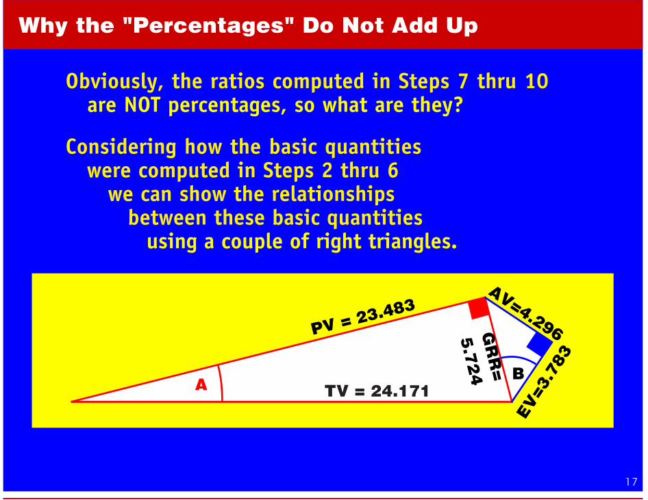
Obviously, the ratios computed in Steps 7 thru 10 are NOT percentages, so what are they?
TV = 24.171
PV = 23.483
GR
R=
5.7
24
AB
EV=3
.783
AV=4.296
Considering how the basic quantities were computed in Steps 2 thru 6 we can show the relationships between these basic quantities using a couple of right triangles.

18
Why the "Percentages" Do Not Add Up
5.724 3.78324.171 5.724
%EV100
= = (Sine A)(Cosine B) = 0.1565
5.724 4.29624.171 5.724
%AV100
= = (Sine A)(Sine B) = 0.1777
5.724 24.171
%GRR100
= = (Sine A) = 0.2368
TV = 24.171
PV = 23.483
GR
R=
5.7
24
AB
EV=3
.783
AV=4.296

19
Why the "Percentages" Do Not Add Up
23.483 24.171
%PV100
= = (Cosine A) = 0.9715
While these ratios were interpreted as proportions,they are clearly trigonometric functions,and that is why the ratios do not add up.
TV = 24.171
PV = 23.483
GR
R=
5.7
24
AB
EV=3
.783
AV=4.296

20
A set of ratios will be proportions if and only if the common denominator is the sum of the numerators.
Why the "Percentages" Do Not Add Up
aa+b+c
ba+b+c
ca+b+c
= 1+ +
TV = EV + AV + PV2 2 2 2
It is the additivity of the numerators that is the essence of proportions.
And in an R&R study it is not the standard deviations,
but rather the variances that are additive.

21
An Honest Gauge R&R Study
TV = EV + AV + PV2 2 2 2
Using the relationship between the variances seen in Step 6:
and dividing both sides by the total variance:
we discover the true proportions inherent in this problem.
TV EV AV PV2 2 2 2
TV 2 TV 2 TV 2 TV 2= + + = 1

22
An Honest Gauge R&R Study
Therefore, the Repeatability actually consumes
EVTV 2
2100 = 100
EV = 3.783 milsAV = 4.296 milsGRR = 5.724 milsPV = 23.483 milsTV = 24.171 mils
3.78324.1712
2= 2.4%
2.4% of the Total Variation,
rather than the 15.7% erroneously found earlier.
Step H7

23
An Honest Gauge R&R Study
The Reproducibility actually consumes
AVTV 2
2100 = 100 4.296
24.1712
2= 3.2%
EV = 3.783 milsAV = 4.296 milsGRR = 5.724 milsPV = 23.483 milsTV = 24.171 mils
3.2% of the Total Variation,
rather than the 17.8% erroneously found earlier.
2.4+3.2
5.6
Step H8

24
An Honest Gauge R&R Study
So that the Combined R&R actually consumes
5.6% of the Total Variation, rather than the 23.7% erroneously found earlier, and these proportions actually add up, as proportions should.
GRRTV 2
2100 = 100 5.724
24.1712
2= 5.6%
EV = 3.783 milsAV = 4.296 milsGRR = 5.724 milsPV = 23.483 milsTV = 24.171 mils
100.0- 5.694.4
Step H9
wro
ngrig
ht
2.4+ 3.2
5.6
15.7+ 17.8
23.7

25
An Honest Gauge R&R Study
EV = 3.783 milsAV = 4.296 milsGRR = 5.724 milsPV = 23.483 milsTV = 24.171 mils
And the Product Variation actually consumes
94.4% of the Total Variation, rather than the 97.2% erroneously found earlier.
PVTV 2
2100 = 100 23.483
24.1712
2= 94.4%
2.4%+3.2%
+94.4%100.0%
Now we have properly accounted for the componentsof the total variation.
RepeatabilityReproducibilityProduct VariationTotal Variation
Step H10

26
What Can You Learn From a Gauge R&R Study?
Repeatablity
Reproducibility
Combined R&R
Product Variation
15.7%
17.8%
23.7%
97.2%
2.4%
3.2%
5.6%
94.4%
TraditonalGauge R&R
Values
HonestGauge R&R
Values

27
What Can You Learn From a Gauge R&R Study?
Repeatablity
Reproducibility
Combined R&R
Product Variation
The Truth
2.4%
3.2%
5.6%
94.4%
By ignoring the Pythagorean Theorem
the Gauge R&R Study converts good data
into values that are hopelessly flawed,
resulting in an analysis where
virtually nothing is true, correct, or useful.
WRONGWRONG
WRONG
WRONG
Gauge R&R
15.7%
17.8%
23.7%
97.2%

28
The Intraclass Correlation
1921
1962
Fisher
R&R
In 1921 Sir Ronald Fisher introduced a theoretically sound and easy to understand way of characterizing the relative utility of a measurement system for a particular application.
This is the Intraclass Correlation, ρ which may be estimated using the value from Step H10:
PVTV
= Est. Intraclass Correlation2
2
= 0.944

29
The Intraclass Correlation
PVTV
= Est. Intraclass Correlation2
2 = 0.944
Clearly the Intraclass Correlation representsthat proportion of the total variation
that is attributable to variation in the product stream.
It also represents the correlation betweentwo measurements of the same thing,
hence the name of intraclass correlation.
This is the appropriate metric for characterizingthe relative utility of a measurement system.

30
First Class Monitors
When the Intraclass Correlation exceeds 80%the measurement system will provide a First Class Monitor.
With First Class Monitorssignals coming from
the production process will be attenuated
by less than 10 percentdue to the effects
of measurement error.
100%
90%
80%
70%
60%
50%
40%
30%
20%
10%
1.00 0.90 0.80
Intraclass Correlation
Sig
na
l S
ten
gth
IC > 80%
PVTV
2
2 = 0.944

31
First Class Monitors
1.00 .80 .20.50
Intraclass Correlation.0
0.0
1.00.90.80.70.60.50.40.30.20.1
Rule I
Rules I, II, III, IV
At
Le
ast
99
%
Pro
babilit
y of
Dete
cti
on
for
Thre
e S
td. E
rror
Shif
t
IC > 80%
When placed on a Process Behavior Chart,First Class Monitorswill have betterthan a 99% chanceof detecting a threestandard error shiftin the productionprocess usingDetection Rule One.
PVTV
= Est. Intraclass Correlation2
2 = 0.944

32
When the Intraclass Correlation is between 80% and 50%the measurement system will provide a Second Class Monitor.
With a Second Class Monitorany signals coming from the production process
will be attenuated by 10 to 30 percentdue to the effects of measurement error.
Second Class Monitors
100%
90%
80%
70%
60%
50%
40%
30%
20%
10%
0.80 0.70 0.60 0.50
Intraclass Correlation
Sig
na
l S
ten
gth
80% > IC > 50%

33
When used with a Process Behavior Chart,Second Class Monitors will still have betterthan an 88% chance of detecting athree standard error shift in the processusing Detection Rule One alone.
Moreover, theyare virtually certain to detecta three standard error shift in the processusing Detection Rules 1, 2, 3, and 4.
Second Class Monitors
1.00 .80 .20.50
Intraclass Correlation.0
0.0
1.00.90.80.70.60.50.40.30.20.1
Rule I
Rules I, II, III, IV
At
Le
ast
88
%
Pro
babilit
y of
Dete
cti
on
for
Thre
e S
td. E
rror
Shif
t
80% > IC > 50%

34
Third Class Monitors
When the Intraclass Correlation is between 50% and 20%the measurement system will provide a Third Class Monitor.
With a Third Class Monitorany signals coming from the production process
will be attenuated by 30 to 55 percentdue to the effects of measurement error.
100%
90%
80%
70%
60%
50%
40%
30%
20%
10%
0.50 0.40 0.30 0.20
Intraclass Correlation
Sig
na
l S
ten
gth
50% > IC > 20%

35
Even though signals from the production process will be attenuated by 30 to 55 percent,when aThird Class Monitoris placed on aProcess BehaviorChart it will still have better thana 91% chance of detecting a three standard error shift using Detection Rules 1, 2, 3, and 4.
Third Class Monitors
1.00 .80 .20.50
Intraclass Correlation.0
0.0
1.00.90.80.70.60.50.40.30.20.1 Rule I
Rules I, II, III, IV
At
Le
ast
91
%
Pro
babilit
y of
Dete
cti
on
for
Thre
e S
td. E
rror
Shif
t
50% > IC > 20%

36
Fourth Class Monitors
When the Intraclass Correlation is below 20%the measurement system will provide a Fourth Class Monitor.
100%
90%
80%
70%
60%
50%
40%
30%
20%
10%
0.20 0.10 0.00
Intraclass Correlation
Sig
na
l S
ten
gth
With a Fourth Class Monitorany signals coming fromthe production process
will be attenuatedby more than 55%
due to the dominatingeffects of measurement
error.
20% > IC

37
Fourth Class Monitors
Any use of a Fourth Class Monitor is an act of desperation.
1.00 .80 .20.50
Intraclass Correlation.0
0.0
1.00.90.80.70.60.50.40.30.20.1 Rule I
Rules I, II, III, IV
Pro
babilit
y of
Dete
cti
on
for
Thre
e S
td. E
rror
Shif
t
ProbabilitiesRapidlyVanishwith
FourthClass
Monitors
20% > IC
With a Fourth Class Monitor the chances of detecting athree standard error shift using a Process Behavior Chartwill rapidly vanishas the measurementscome to have lessand less informationabout the productionprocess.

38
The Four Classes of Process Monitors
Thus the Intraclass Correlation characterizesthe relative utility of a measurement system
for a given application.
It is theoretically sound, it is easy to interpret, and
it results in a practical classification scheme.
PVTV
= Estimated Intraclass Correlation2
2

39
The Gauge R&R Guidelines
How are these Four Classes of monitors related to the Guidelines given in a Traditional Gauge R&R Study?
These Guidelines are generally applied in the form:
%GRR values that are less than 10% are good,%GRR values between 10% and 30% are marginal, and%GRR values that exceed 30% are unacceptable.
GRRTV
[ EV + AV ]TV
= 2 2 0.5
= [ 1 – IC ] 0.5%GRR100
=
To compare these guidelines with the Four Classes we need to know how %GRR is related to IC.

40
The Gauge R&R Guidelines
IC = 1 – 2%GRR
100[ ]
So that a %GRR value of 10% corresponds to an Intraclass Correlation of 0.99.
And a %GRR value of 30% corresponds to an Intraclass Correlation of 0.91.
0% 10% 20% 30% 40% 50% 60% 70% 80% 90% 100%
100% 90% 80% 70% 60% 50% 40% 30% 20% 10% 0%
Values of the Intraclass Correlation Coefficient
According to the Arbitrary Gauge R&R Guidelines Measurement Systems Fall into Three Categories
Values of the Traditional Gauge R&R Ratio
"Good" "Marginal" "In Need of Improvement"
GRR
IC

41
The Four Classes of Monitors
First Class Monitors will have %GRR values below 0.447.
Second Class Monitors will have %GRR values below 0.707.
Third Class Monitors will have %GRR values below 0.894.
100% 90% 80% 70% 60% 50% 40% 30% 20% 10% 0%
0% 10% 20% 30% 40% 50% 60% 70% 80% 90% 100%
FourthClass
Monitors
First Class Monitors
Third Class Monitors
GRR
IC
On the other hand:
But the best way to see the difference between these two characterizations of relative utility is to consider their impact upon Process Capability.
Second Class Monitors

42
Quantifying Process Improvements
For the Gasket Thickness the specs are 145 to 225 mils.
With a TV value of 24.171 mils we would estimate the current Capability Ratio to be:
Cp = Upper Spec – Lower Spec6 Total Variation
225 – 1456 (24.171)
= 0.55Cp =
With an IC of 0.944 we have a First Class Monitor, yet according to the Gauge R&R Study, with a %GRR of 23.7% we have a marginal measurement system.How much improvement can be tracked according to these two different approaches to R&R?

43
Quantifying Process Improvements
Any reduction in the Product Variation will result in an increase in the Capability Ratio; an increase in the %GRR value; and a decrease in the Intraclass Correlation.
For the Gasket Thicknesses: If the Product Variation dropped from 23.48 to 18.20, the Capability Ratio would change from 0.55 to 0.70, the %GRR value would become 30%, and the Intraclass Correlation would drop to 0.91.
At this point the Gauge R&R Study would condemn the measurement system.
Therefore, Gauge R&R Studies offer little opportunity to quantify process improvements.
44
Quantifying Process Improvements
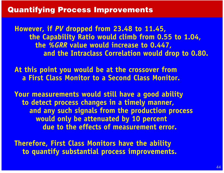
However, if PV dropped from 23.48 to 11.45, the Capability Ratio would climb from 0.55 to 1.04, the %GRR value would increase to 0.447, and the Intraclass Correlation would drop to 0.80.
At this point you would be at the crossover from a First Class Monitor to a Second Class Monitor.
Your measurements would still have a good ability to detect process changes in a timely manner, and any such signals from the production process would only be attenuated by 10 percent due to the effects of measurement error.
Therefore, First Class Monitors have the ability to quantify substantial process improvements.

45
Quantifying Process Improvements
Furthermore, if PV dropped from 11.45 to 5.72, the Capability Ratio would climb from 1.04 to 1.65, the %GRR value would increase to 0.707, and the Intraclass Correlation would drop to 0.50.
At this point you would be at the crossover from a Second Class Monitor to a Third Class Monitor.
Your measurements would still have a reasonable ability to detect process changes in a timely manner, and any such signals from the production process would only be attenuated by 30 percent due to the effects of measurement error.
Therefore, Second Class Monitors still have the ability to quantify substantial process improvements.

46
Quantifying Process Improvements
Finally, if PV dropped from 5.72 to 2.86, the Capability Ratio would climb from 1.65 to 2.08, the %GRR value would increase to 0.894, and the Intraclass Correlation would drop to 0.20.
At this point you would be at the crossover from a Third Class Monitor to a Fourth Class Monitor.
Signals from the production process would be attenuated by 55 percent and the measurement system would have little remaining utility.
Therefore, Third Class Monitors still have the ability to quantify process improvements and detect process changes.
47
Quantifying Process Improvements
11.45
5.722.86
23.48
52%
76%88%
23.48
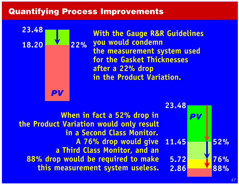
18.20 22%With the Gauge R&R Guidelinesyou would condemn the measurement system usedfor the Gasket Thicknessesafter a 22% drop in the Product Variation.
When in fact a 52% drop in the Product Variation would only result
in a Second Class Monitor. A 76% drop would give
a Third Class Monitor, and an88% drop would be required to make
this measurement system useless.
PV
PV

48
Quantifying Process Improvements
Cp80 = USL – LSL6 √5 GRR
Thus, by computing the Crossover Capabilities you candetermine the ability of a particular measurement system
to detect improvements in a particular process.
Cp50 = USL – LSL6 √2 GRR
Cp20 = USL – LSL6 √1.25 GRR
First Class Monitor
Second Class Monitor
Third Class Monitor
Fourth Class Monitor
IncreasingCapability

49
Lessons Learned
Hence, we must conclude that the sole purpose of a Gauge R&R Study
is to condemn the measurement process.
Not only is the %GRR ratio inflated by being computed incorrectly,
but the guidelines used to interpret this ratioare excessively conservative,
and do not even begin to definethe relative utility of the measurement system.
0% 10% 20% 30% 40% 50% 60% 70% 80% 90% 100%
100% 90% 80% 70% 60% 50% 40% 30% 20% 10% 0%
Values of the Intraclass Correlation Coefficient
According to the Arbitrary Gauge R&R Guidelines Measurement Systems Fall into Three Categories
Values of the Traditional Gauge R&R Ratio
"Good" "Marginal" "In Need of Improvement"
GRR
IC

50
Lessons Learned
It has been demonstrated that:
The ratios computed in Steps 7, 8, 9, & 10 of a Traditonal Gauge R&R Study do not represent what they are said to represent. (This is true for steps 11 through 14 as well.)
The Guidelines used by Traditional Gauge R&R Studies are so conservative that they are nonsense.
The proper measure of relative utility is the Intraclass Correlation, which can be used to define four clear and meaningful classes of process monitors.

51
The Choice is Clear
Do you want to condemn your measurement systems?
Or would you prefer to use your less-than-perfect data
to operate and improve your processes?
0% 10% 20% 30% 40% 50% 60% 70% 80% 90% 100%
100% 90% 80% 70% 60% 50% 40% 30% 20% 10% 0%
Values of the Intraclass Correlation Coefficient
Values of the Traditional Gauge R&R Ratio
"Good" "Marginal" "In Need of Improvement"
GRR
IC
100% 90% 80% 70% 60% 50% 40% 30% 20% 10% 0%
0% 10% 20% 30% 40% 50% 60% 70% 80% 90% 100%
FourthClass
Monitors
First Class Monitors
Third Class Monitors
GRR
IC
Second Class Monitors
52
AVTV 2
2
GRRTV 2
2
PVTV 2
2
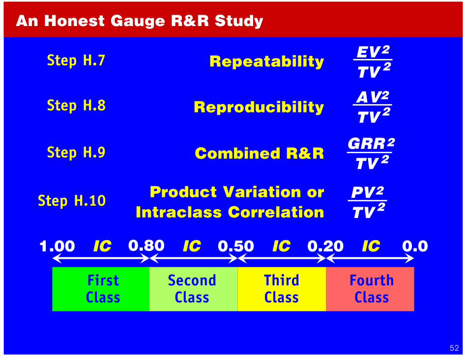
An Honest Gauge R&R Study
EVTV 2
2Repeatability
Reproducibility
Combined R&R
Product Variation orIntraclass Correlation
Step H.7
Step H.8
Step H.9
Step H.10
FirstClass
SecondClass
ThirdClass
FourthClass
0.80 0.50 0.201.00 0.0IC IC IC IC

53
An Honest Gauge R&R Study
Chance ofDetecting a
3 Std. Error Shift
More than 99%with Rule One
More than 88%with Rule One
More than 91%w/Rules 1,2,3,4
RapidlyVanishes
Attenuation of Process
Signals
Less than 10 Percent
10 Percent to30 Percent
30 Percent to55 Percent
More than55 Percent
First ClassMonitors
Second ClassMonitors
Third ClassMonitors
Fourth ClassMonitors
1.00
0.80
0.50
0.20
0.00
IC
Cp80
Cp50
Cp20
CannotTrack
To
TrackProcessImprov.
To
To


![Gauge & R&R [Repeatability & Reproducibility] Analysis](https://img.pdfslide.us/doc/110x75/54becf3e4a7959a67f8b4696/gauge-rr-repeatability-reproducibility-analysis.jpg)