Process algebras in systems biology

Federica Ciocchetta1 and Jane Hillston1

Laboratory for Foundations of Computer Science, The University of Edinburgh,Edinburgh EH9 3JZ, Scotland

(fchiocche,jeh)@inf.ed.ac.uk

Abstract. In this work we present Bio-PEPA, a process algebra for the modellingand the analysis of biochemical networks. It is a modification of PEPA, originallydefined for the performance analysis of computer systems, in order to handlesome features of biological models, such as stoichiometry and the use of gen-eral kinetic laws. The domain of application is the one of biochemical networks.Bio-PEPA may be seen as an intermediate, formal, compositional representationof biological systems, on which different kinds of analysis can be carried out.Bio-PEPA is enriched with some notions of equivalence. Specifically, the iso-morphism and strong bisimulation for PEPA have been considered. Finally, weshow the translation of three biological models into the new language and wereport some analysis results.

1 Introduction

In recent years there has been increasing interest in the application of process algebrasin the modelling and analysis of biological systems [60, 26, 28, 58, 19, 49, 14]. Processalgebras have some interesting properties that make them particularly useful in describ-ing biological systems. First of all, they offer compositionality, i.e. the possibility ofdefining the whole system starting from the definition of its subcomponents. Secondly,process algebras give a formal representation of the system avoiding ambiguity. Thirdly,biological systems can be abstracted by concurrent systems described by process alge-bras: species may be seen as processes that can interact with each other and reactionsmay be modelled using actions. Finally, different kinds of analysis can be performed ona process algebra model. These analyses provide conceptual tools which are comple-mentary to established techniques: it is possible to detect and correct potential inaccu-racies, to validate the model and to predict its possible behaviours.

The process algebra PEPA, originally defined for the performance analysis of com-puter systems, has been recently applied in the context of signalling pathways [14, 15].Two different approaches have been proposed: one based on reagents (the so-calledreagent-centric view) and another based on pathways (pathway-centric view). In bothcases the species concentrations are discretized into levels, each level abstracting aninterval of concentration values. In the reagent-centric view the PEPA sequential com-ponents represent the different concentration levels of the species. In this approach theabstraction is “processes as species” and not “processes as molecules”, as in other pro-cess algebras such as the π-calculus and Beta-binders [60, 58]. In the pathway-centricapproach we have a more abstract view: the processes represent sub-pathways. Here

multiple copies of components represent levels of concentration. The two views havebeen shown to be equivalent [15].

Even though PEPA has proved useful in studying signalling pathways, it does notallow us to represent all the features of biological networks. The main difficulties arethe definition of stoichiometric coefficients (i.e. the coefficients used to show the quan-titative relationships of the reactants and products in a biochemical reaction) and therepresentation of kinetic laws. Indeed, stoichiometry is not represented explicitly andthe reactions are assumed to be elementary (with constant rate). The problem of extend-ing to the domain of kinetic laws beyond basic mass-action (hereafter called generalkinetic laws) is particularly relevant, as these kinds of reactions are frequently found inthe literature as abstractions of complex situations whose details are unknown. Reduc-ing all reactions to the elementary steps is complex and often impractical. This prob-lem impacts also on other process algebras. Indeed, generally they rely on Gillespie’sstochastic simulation for analysis which considers only elementary reactions. Some re-cent works have extended the approach of Gillespie to deal with complex reactions [1,17] but these extensions are yet to be reflected in the work using process algebras. Pre-vious work concerning the use of general kinetic laws in process algebras and formalmethods was presented in [9, 20]. These are discussed in Section ??.

In this chapter we make a tutorial introduction to Bio-PEPA, a new language for themodelling and analysis of biochemical networks. A preliminary version of the languagewas proposed in [22], with full details presented in [?]. Here, in addition to defining thelanguage we illustrate its use with a number of examples.

Bio-PEPA is based on the reagent-centric view in PEPA, modified in order to repre-sent explicitly some features of biochemical models, such as stoichiometry and the roleof the different species in a given reaction. A major feature of Bio-PEPA is the intro-duction of functional rates to express general kinetic laws. Each action type representsa reaction in the model and is associated with a functional rate.

The idea underlying our work is represented schematically in the diagram in Fig. 1.The context of application is biochemical networks. Broadly speaking, biochemical net-

Bio−PEPA SYSTEM BIOCHEMICAL NETWORKS

(Gillespie)

CTMC (with levels)

ODEs

(SBML, KEGG,...)

(model checking)

Stochastic simulation

PRISM

Fig. 1. Schema of the Bio-PEPA framework

works consist of some chemical species, which interact with each other through chem-ical reactions. The dynamics of reaction are described in terms of some kinetic laws.

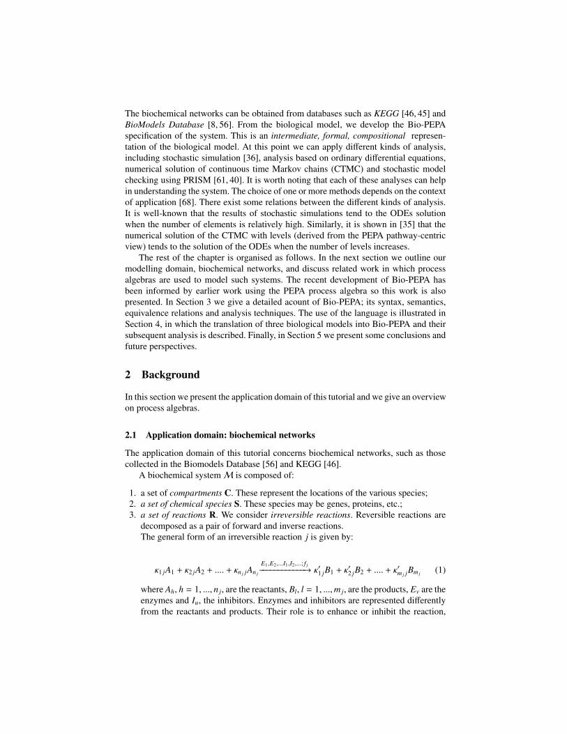
The biochemical networks can be obtained from databases such as KEGG [46, 45] andBioModels Database [8, 56]. From the biological model, we develop the Bio-PEPAspecification of the system. This is an intermediate, formal, compositional represen-tation of the biological model. At this point we can apply different kinds of analysis,including stochastic simulation [36], analysis based on ordinary differential equations,numerical solution of continuous time Markov chains (CTMC) and stochastic modelchecking using PRISM [61, 40]. It is worth noting that each of these analyses can helpin understanding the system. The choice of one or more methods depends on the contextof application [68]. There exist some relations between the different kinds of analysis.It is well-known that the results of stochastic simulations tend to the ODEs solutionwhen the number of elements is relatively high. Similarly, it is shown in [35] that thenumerical solution of the CTMC with levels (derived from the PEPA pathway-centricview) tends to the solution of the ODEs when the number of levels increases.

The rest of the chapter is organised as follows. In the next section we outline ourmodelling domain, biochemical networks, and discuss related work in which processalgebras are used to model such systems. The recent development of Bio-PEPA hasbeen informed by earlier work using the PEPA process algebra so this work is alsopresented. In Section 3 we give a detailed acount of Bio-PEPA; its syntax, semantics,equivalence relations and analysis techniques. The use of the language is illustrated inSection 4, in which the translation of three biological models into Bio-PEPA and theirsubsequent analysis is described. Finally, in Section 5 we present some conclusions andfuture perspectives.

2 Background

In this section we present the application domain of this tutorial and we give an overviewon process algebras.

2.1 Application domain: biochemical networks

The application domain of this tutorial concerns biochemical networks, such as thosecollected in the Biomodels Database [56] and KEGG [46].

A biochemical systemM is composed of:

1. a set of compartments C. These represent the locations of the various species;2. a set of chemical species S. These species may be genes, proteins, etc.;3. a set of reactions R. We consider irreversible reactions. Reversible reactions are

decomposed as a pair of forward and inverse reactions.The general form of an irreversible reaction j is given by:

κ1 jA1 + κ2 jA2 + .... + κn j jAn j

E1,E2,...I1,I2,...; f j−−−−−−−−−−−−→ κ′1 jB1 + κ

′2 jB2 + .... + κ

′m j jBm j (1)

where Ah, h = 1, ..., n j, are the reactants, Bl, l = 1, ...,m j, are the products, Ev are theenzymes and Iu, the inhibitors. Enzymes and inhibitors are represented differentlyfrom the reactants and products. Their role is to enhance or inhibit the reaction,

respectively. We call species that are involved in a reaction without changing theirconcentration (i.e. enzymes and inhibitors) modifiers. The parameters κh j and κ′l j arethe stoichiometry coefficients. These express the degree to which species participatein a reaction. The dynamics associated with the reaction is described by a kineticlaw f j, depending on some parameters and on the concentrations of some species.

The best known kinetic law is mass-action: the rate of the reaction is proportional to theproduct of the reactants’ concentrations. In published models it is common to find gen-eral kinetic laws, which describe approximations of sequences of reactions. They areuseful when it is difficult to derive certain information from the experiments, e.g. the re-action rates of elementary steps, or when there are different time-scales for the reactions.Generally these laws are valid under some conditions, such as the quasi-steady-state as-sumption (QSSA). This describes the situation where one or more reaction steps may beconsidered faster than the others and so the intermediate elements can be considered tobe constant. There is a long list of kinetic laws; for details see [65].

2.2 Overview on Process algebras

Process algebras are calculi that were introduced in computer science to specify for-mally and model concurrent systems [51, 43]. They have been used to deal with com-plex systems characterized by concurrency, communication, synchronization and non-determinism. Process algebras offer several attractive features which are not necessarilyavailable in existing performance modelling paradigms. The most important of theseare compositionality, the ability to model a system as the interaction of its subsystems,formality, giving a precise meaning to all terms in the language, and abstraction, theability to build up complex models from detailed components but disregarding internalbehaviour when it is appropriate to do so.

The most widely known process algebras are Milner’s Calculus of Communicat-ing Systems (CCS) [51] and Hoare’s Communicating Sequential Processes (CSP) [43].Models in CCS and CSP have been used to establish the correct behaviour of complexsystems by deriving qualitative properties such as freedom from deadlock or livelock.

Process algebras are defined by a simple syntax and semantics. The semantics isgiven by axioms and inference rules expressed in an operational way [57]. A systemis defined as a collection of agents which execute atomic actions. Some operators areintroduced for combining the primitives. For instance in CCS the main operators are:

– prefix a.P after action a the agent– parallel composition P|Q agents P and Q proceed in parallel– choice P + Q the agent behaves as P or Q– restriction A\M the set of labels M is hidden– relabelling A[a1/a0, ..] in this agent label a1 is renamed a0

– the null agent 0 this agent cannot act (deadlock)

One of the main peculiarities of process algebras is the possibility to express com-munication between two processes. In some cases, such as CCS [51] and π-calculus[52], a communication between two parallel processes is enabled if one process can

perform an action a (receive) and the other process can perform the complementary ac-tion a (send). So the actions must be complementary (input-output) and share the samename (a in the case considered). The resulting communication has the distinguishedlabel τ, that indicates an internal (invisible) action. A peculiarity of π-calculus withrespect to CCS is the possibility to represent name-passing: communicating processescan exchange names over channels and consequently they may change their interactiontopology.

The communication mechanism in CSP is different from the one described aboveas there is no notion of complementary actions. In CSP two agents communicate bysimultaneously executing actions with the same label. Since during the communicationthe joint action remains visible to the environment, it can be reused by other concur-rent processes so that more than two processes can be involved in the communication(multiway synchronisation).

The analysis of the behaviours of the model, represented in a formal language, isgenerally produced through a Labeled Transition System (LTS). From this a derivativetree or graph in which language terms form the nodes and transitions are the arcs, maybe constructed. This structure is a useful tool for reasoning about agents and the systemsthey represent. It is also the basis of the bisimulation style of equivalence. In this styleof equivalence, the actions of an agent characterise it, so two agents are considered tobe equivalent if they are observed to perform exactly the same actions. Strong and weakforms of equivalence are defined depending on whether the internal actions of an agentare deemed to be observable.

In CCS and CSP, since the objective is qualitative analysis rather than quantitative,time and uncertainty are abstracted away. In the last decade various suggestions for in-corporating time and probability into these formalisms have been investigated (see [54]for an overview of process algebras with time). For example, Temporal CCS (TCCS)[53] extends CCS with fixed delays and wait-for synchronisation (asynchronous wait-ing). Note that most of the timed extensions, including TCCS, retain the assumptionthat actions are instantaneous and regard time progression as orthogonal to the activityof the system. These assumptions make such models unsuitable for performance analy-sis. Probabilistic extensions of process algebras, such as PCCS [44], allow uncertaintyto be quantified using a probabilistic choice combinator. In this case a probability isassociated with each possible outcome of a choice.

In the early 1990s several stochastic extensions of process algebra (stochastic pro-cess algebras or SPA), have been introduced. SPA add quantification to models makingthem suitable for performance modelling. The general idea is to associate a randomvariable with all the actions of the calculus. In most cases, the random variables areassumed to be exponentially distributed and a rate is added to each prefix to representthe parameter of the exponential distribution that describes the dynamic behaviour ofthe associated action. A race condition has then been considered: all the activities thatare enabled in a given state compete and the fastest one succeeds. The choice of expo-nential distribution permits to associate the process algebra model to a continuous timeMarkov chain (CTMC) and therefore to carry out analysis based on this approach. Some

examples of SPA are TIPP [38], EMPA1 [?,5], PEPA [42], SPADE2 [67] and Stochasticπ-calculus [59].

2.3 Process algebras in systems biology

Recently, as a response to the need of modeling the dynamics of complex biologicalsystems, there have been some applications of process calculi in systems biology [60,62, 28, 58, 27, 18, 19, 14]. These techniques are appropriate for describing formally andanalyzing a biological system as a whole and for reasoning about protein/gene inter-actions. Indeed, there exists a strong correspondence between concurrent systems de-scribed by process algebras and biological ones: biological entities may be abstracted asprocesses that can interact each other and reactions may be modeled by using actions.

Process calculi have some properties that make them useful for studying biologicalsystems:

– they allow the formal specification of the system;– they offer different levels of abstraction for the same biological system;– they can make interactions explicit, in particular biological elements may be seen

as entities that interact and evolve;– they support modularity and compositionality;– they provide well-established techniques for reasoning about possible behaviours.

They may be used not only for the simulation of the system, but also for the verifi-cation of formal properties and for behaviour comparison through equivalences.

Several process calculi have been proposed in biology. Each of them has different prop-erties able to render different aspects of biological phenomena. They may be dividedinto two main categories:

– calculi defined originally in computer science and then applied in biology, such asthe biochemical stochastic π-calculus, [60], CCS-R [28], PEPA [42];

– calculi defined ad hoc by observing biological structures and phenomena, such asBioAmbients [19], Brane Calculi [18], κ-calculus [27], and Beta-binders [58].

One of the first process algebras used in systems biology is the biochemical π-calculus [60], a variant of the π-calculus defined to model biological systems. The un-derlying idea of application of the π-calculus to biology is the molecule-as-computationabstraction [63, 60]: each biological entity and interaction is associated with a specifica-tion in the calculus. Specifically, molecules are modeled as processes, interaction capa-bilities as channels, interactions as communications between processes, modificationsas state and channel changes and, finally, compartments and membranes as restrictions.Two stochastic simulation tools based on Gillespie [36] have been defined (BIOSPI[6] and SPIM [66]), various applications have been shown [50, 26, 49, 21] and somemodified versions have been proposed (e.g. SPICO[48] and Sp@ [69]).

1 Originally called simply MPA.2 Originally called CCS+.

CCS-R [28] is a variant of CCS with new elements that allows the manage of re-versibility. The interactions are described in terms of binary synchronized communica-tions, similarly to π-calculus. The successor of CSS-R is the Reversible CCS (RCCS)[31]. This calculus allows processes to backtrack if this is in agreement with a notionof casual equivalence defined in the paper.

Another language used for the modelling of biological systems is the κ-calculus [27],based on the description of protein interactions. Processes describe proteins and theircompounds, a set of processes models solutions and protein behaviour is given by aset of rewriting rules, driven by suitable side-conditions. The two main rules concernactivation and complexation. A stochastic simulator for κ-calculus is described in [30].A few applications are reported, as in [29].

Beta-binders [58, 64] is an extension of the π-calculus inspired by biological phe-nomena. This calculus is based on the concept of bio-process, a box with some sites(beta-binders) to express the interaction capabilities of the element, in which π-likeprocesses (pi-processes) are encapsulated. Beta-binders enrich the standard π-calculuswith some constructs that allow us to represent biological features, such as the joinbetween two bio-processes, the split of one bio-process into two, the change of the bio-process interface by hiding, unhiding and exposing a site. The Beta Workbench [64] isa collection of tools for the modelling, simulation and analysis of Beta-binders system.The BetaWB simulator is based on a variant of Gillespie’s algorithm.

In most of the calculi considered it is not possible to represent all the featuresof biochemical networks. Generally the kinetic laws are assumed to be mass-actionand reactions can have at most two reactants. Indeed these calculi refer to the stan-dard Gillespie’s algorithm for the analysis and this assumes elementary reactions (i.e.monomolecular or bimolecular) with constant rates. Furthermore, biological reactionsare abstracted as communications/interactions between agents and in some process al-gebras such as π-calculus, CCS and Beta-binders these actions are pairwise. There-fore multiple-reactant multiple-product reactions cannot be modelled in these calculi.In order to represent multiple-reactant multiple-product reactions π-calculus and Beta-binders have been enriched with transactions [24, 25].

A first proposal to deal with general kinetic laws has been shown in [9]. The authorsof [9] present a stochastic extension of Concurrent Constraint Programming (CCP) andshow how to apply it in the case of biological systems. Here each species is representedby a variable and the reactions are expressed by constraints on these variables. Thedomain of application is extended to any kind of reactions and the rate can be expressedby a generic function.

The possibility to represent general kinetic laws is also offered by BIOCHAM [20],a programming environment for modeling biochemical systems, making simulationsand querying the model in temporal logic. This language is not a process algebra, but itis based on a rule-based language for modeling biochemical systems, in which speciesare expressed by objects and reactions by reaction rules.

Finally, some calculi has been defined to model compartments and membranes.Here we describe briefly Bio-ambients [19] and Brane calculi [18]. Bio-ambients iscentered on ambients, bounded places where processes are contained and where com-munication may happen. Ambients can be nested and organized as a hierarchy. This

hierarchy may be modified by suitable operations that have a biological interpretation.It is possible to have an enter n and an exit n primitives to move an ambient into or out ofanother ambient or a merge+ n/merge- n for merging two ambients together. Ambientscontain compounds that interact via communications. Bio-ambients have been used tomodel compartments in BIOSPI [6]. A stochastic semantics for Bio-ambients has beenformalized in [10]. There are few applications, for instance [3].

In Brane calculi [18] a system consists of nested membranes, which are collectionsof actions. Membranes may shift, merge, break apart and may be replenished, leadingto very expressive models, in which actions occur on membranes. Membranes may beseen as oriented objects that must obey to some restrictions on orientation. In partic-ular they must preserve bitonality, which requires nested membranes to have oppositeorientations.

2.4 PEPA and biological systems

PEPA is a stochastic process algebra originally defined for the performance modellingof systems with concurrent behaviour [42]. In PEPA each action is assumed to have aduration, represented by a random variable with a negative exponential distribution. Weinformally introduced the syntax of the language below. For more details see [42].

Prefix The basic term is the prefix combinator (α, r).S . It denotes a component whichhas action of type α and an exponentially distributed duration with parameter r(mean duration 1/r), and it subsequently behaves as S .

Choice The component S + R represents a system which may behave either as S oras R. The activities of both S and R are enabled. The first activity to completedistinguishes one of them and the other is discarded.

Constant Constants are components whose meaning is given by a defining equation

Cde f= S . They allow us to assign names to patterns of behaviour associated with

components.Hiding In S/H the set H identifies those activities which can be considered internal

or private to the component S .Cooperation The term P BC

LQ denotes cooperation between P and Q over the coop-

eration set L, that determines those activities on which the cooperands are forcedto synchronise. PEPA supports multiway synchronisation between components: theresult of synchronising on an activity α is thus another α, available for further syn-chronisation. For action types not in L, the components proceed independently andconcurrently with their enabled activities. In the context of performance evaluationthe rate for the synchronised activities is the minimum of the rates of the synchro-nising activities.

Recently, PEPA has been applied to the modelling and analysis of signalling path-ways. A first study concerns the influence of the Raf Kinase Inhibitor Protein (RKIP)on the Extracellular signal Regulated Kinase (ERK) [14], whereas in [15] the PEPAsystem for Schoeberl’s model [32] involving the MAP kinase and EFG receptors is re-ported. In [14] two different modelling styles have been proposed, one based on thereagent-centric view and the other on the pathway-centric view. The former focuses on

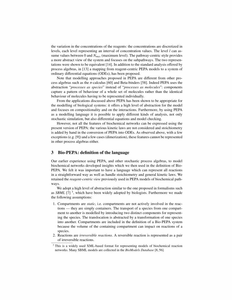
the variation in the concentrations of the reagents: the concentrations are discretized inlevels, each level representing an interval of concentration values. The level l can as-sume values between 0 and Nmax (maximum level). The pathway-centric style providesa more abstract view of the system and focuses on the subpathways. The two represen-tations were shown to be equivalent [14]. In addition to the standard analysis offered byprocess algebras, in [13] a mapping from reagent-centric PEPA models to a system ofordinary differential equations (ODEs), has been proposed.

Note that modelling approaches proposed in PEPA are different from other pro-cess algebras such as the π-calculus [60] and Beta-binders [58]. Indeed PEPA uses theabstraction “processes as species” instead of “processes as molecules”: componentscapture a pattern of behaviour of a whole set of molecules rather than the identicalbehaviour of molecules having to be represented individually.

From the applications discussed above PEPA has been shown to be appropriate forthe modelling of biological systems: it offers a high level of abstraction for the modeland focuses on compositionality and on the interactions. Furthermore, by using PEPAas a modelling language it is possible to apply different kinds of analysis, not onlystochastic simulation, but also differential equations and model checking.

However, not all the features of biochemical networks can be expressed using thepresent version of PEPA: the various kinetic laws are not considered and stoichiometryis added by hand in the conversion of PEPA into ODEs. As observed above, with a fewexceptions (e.g. [9]) and a few cases (dimerization), these features cannot be representedin other process algebras either.

3 Bio-PEPA: definition of the language

Our earlier experience using PEPA, and other stochastic process algebras, to modelbiochemical networks developed insights which we then used in the definition of Bio-PEPA. We felt it was important to have a language which can represent all reactionsin a straightforward way as well as handle stoichiometry and general kinetic laws. Weretained the reagent-centric view previously used in PEPA models of biochemical path-ways.

We adopt a high level of abstraction similar to the one proposed in formalisms suchas SBML [7] 3, which have been widely adopted by biologists. Furthermore we madethe following assumptions:

1. Compartments are static, i.e. compartments are not actively involved in the reac-tions — they are simply containers. The transport of a species from one compart-ment to another is modelled by introducing two distinct components for represent-ing the species. The translocation is abstracted by a transformation of one speciesinto another. Compartments are included in the definition of a Bio-PEPA systembecause the volume of the containing compartment can impact on reactions of aspecies.

2. Reactions are irreversible reactions. A reversible reaction is represented as a pairof irreversible reactions.

3 This is a widely used XML-based format for representing models of biochemical reactionnetworks. Many SBML models are collected in the BioModels Database [8, 56].

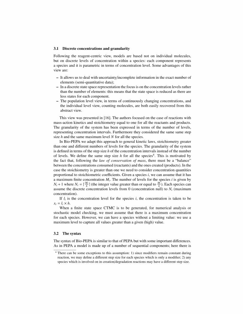
3.1 Discrete concentrations and granularity

Following the reagent-centric view, models are based not on individual molecules,but on discrete levels of concentration within a species: each component representsa species and it is parametric in terms of concentration level. Some advantages of thisview are:

– It allows us to deal with uncertainty/incomplete information in the exact number ofelements (semi-quantitative data);

– In a discrete state space representation the focus is on the concentration levels ratherthan the number of elements: this means that the state space is reduced as there areless states for each component.

– The population level view, in terms of continuously changing concentrations, andthe individual level view, counting molecules, are both easily recovered from thisabstract view.

This view was presented in [16]. The authors focused on the case of reactions withmass-action kinetics and stoichiometry equal to one for all the reactants and products.The granularity of the system has been expressed in terms of the number of levels,representing concentration intervals. Furthermore they considered the same same stepsize h and the same maximum level N for all the species.

In Bio-PEPA we adapt this approach to general kinetic laws, stoichiometry greaterthan one and different numbers of levels for the species. The granularity of the systemis defined in terms of the step size h of the concentration intervals instead of the numberof levels. We define the same step size h for all the species4. This is motivated bythe fact that, following the law of conservation of mass, there must be a “balance”between the concentrations consumed (reactants) and the ones created (products). In thecase the stoichiometry is greater than one we need to consider concentration quantitiesproportional to stoichiometric coefficients. Given a species i, we can assume that it hasa maximum finite concentration Mi. The number of levels for the species i is given byNi + 1 where Ni = d

Mih e (the integer value greater than or equal to Mi

h ). Each species canassume the discrete concentration levels from 0 (concentration null) to Ni (maximumconcentration).

If li is the concentration level for the species i, the concentration is taken to bexi = li × h.

When a finite state space CTMC is to be generated, for numerical analysis orstochastic model checking, we must assume that there is a maximum concentrationfor each species. However, we can have a species without a limiting value: we use amaximum level to capture all values greater than a given (high) value.

3.2 The syntax

The syntax of Bio-PEPA is similar to that of PEPA but with some important differences.As in PEPA a model is made up of a number of sequential components; here there is

4 There can be some exceptions to this assumption: 1) since modifiers remain constant duringreaction, we may define a different step size for each species which is only a modifier; 2) anyspecies which is involved on in creation/degradation reactions may have a different step size.

one sequential component for each species. As we will see, the syntax of Bio-PEPAis designed in order to collect the biological information that we need. For example,instead of a single prefix combinator there are a number of different operators whichcapture the role that the species plays with respect to this reaction.

S ::= (α, κ) op S | S + S | C P ::= P BCL

P | S (l)

where op = ↓ | ↑ | ⊕ | | �.The component S is called sequential component (or species component) and rep-

resents the species. The component P, called a model component, describes the systemand the interactions among components. We suppose a countable set of model com-ponents C and a countable set of action types A. The parameter l ∈ N represents thediscrete level of concentration. The prefix term, (α, κ) op S , contains information aboutthe role of the species in the reaction associated with the action type α:

– (α, κ) is the activity or reaction, where α ∈ A is the action type and κ is the stoi-chiometry coefficient of the species in that reaction; information about the rate ofthe reaction is defined elsewhere (in contrast to PEPA);

– the prefix combinator “op” represents the role of the element in the reaction. Specif-ically, ↓ indicates a reactant, ↑ a product, ⊕ an activator, an inhibitor and � ageneric modifier.

The choice operator, cooperation and definition of constant are unchanged. In con-trast to PEPA the hiding operator is omitted.

In order to fully describe a biochemical network in Bio-PEPA we need to definestructures that collect information about the compartments, the maximum concentra-tions, number of levels for all the species, the constant parameters and the functionalrates which specify the rates of reactions. In the following the function name returnsthe names of the elements of a given Bio-PEPA component.

First of all we define the set of compartments.

Definition 1. Each compartment is described by “V: v unit”, where V is the compart-ment name, “v” is a positive real number expressing the compartment size and the(optional) “unit” denotes the unit associated with the compartment size. The set ofcompartments is denotedV.

In Bio-PEPA compartments are static and they cannot change their structure/size.The set of compartments must contain at least one element. When we have no informa-tion about compartments we add a default compartment whose size is 1 and whose unitdepends on the model.

Definition 2. For each species we define the element C : H,N,M0,M,V, where:

– C is the species component name,– H ∈ N is the step size,– N ∈ N is the maximum level,– M0 ∈ R

+ ∪ { } is the initial concentration,– M ∈ R+ ∪ { } is the maximum concentration,– V ∈ name(V) ∪ { } is the name of the enclosing compartment.

The set of all the elements C : H,N,M0,M,V is denoted N .

In the definition the symbol “ ” denotes the empty string, indicating that the last threecomponents are optional. The initial concentration may added when we want to com-pare our model results with the results in the literature. The maximum concentration isused in the definition of the number of levels, but generally it can be derived from thestep size and the maximum number of levels. Finally, if there is only one compartmentfor all the species in the model we can omit it in the definition of N .

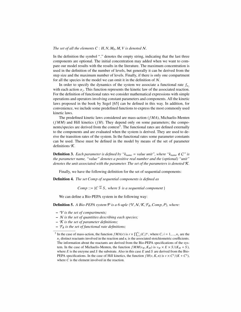
In order to specify the dynamics of the system we associate a functional rate fα j

with each action α j. This function represents the kinetic law of the associated reaction.For the definition of functional rates we consider mathematical expressions with simpleoperations and operators involving constant parameters and components. All the kineticlaws proposed in the book by Segel [65] can be defined in this way. In addition, forconvenience, we include some predefined functions to express the most commonly usedkinetic laws.

The predefined kinetic laws considered are mass-action ( f MA), Michaelis-Menten( f MM) and Hill kinetics ( f H). They depend only on some parameters; the compo-nents/species are derived from the context5. The functional rates are defined externallyto the components and are evaluated when the system is derived. They are used to de-rive the transition rates of the system. In the functional rates some parameter constantscan be used. These must be defined in the model by means of the set of parameterdefinitions K .

Definition 3. Each parameter is defined by “kname = value unit”, where “kname < C” isthe parameter name, “value” denotes a positive real number and the (optional) “unit”denotes the unit associated with the parameter. The set of the parameters is denotedK .

Finally, we have the following definition for the set of sequential components:

Definition 4. The set Comp of sequential components is defined as

Comp ::= {C def= S , where S is a sequential component }

We can define a Bio-PEPA system in the following way:

Definition 5. A Bio-PEPA system P is a 6-uple 〈V,N ,K ,FR,Comp, P〉, where:

– V is the set of compartments;– N is the set of quantities describing each species;– K is the set of parameter definitions;– FR is the set of functional rate definitions;

5 In the case of mass-action, the function f MA(r) is r ×∏n j

i=1(Ci)κi , where Ci i = 1, ..., n j are then j distinct reactants involved in the reaction and κi is the associated stoichiometric coefficients.The information about the reactants are derived from the Bio-PEPA specifications of the sys-tem. In the case of Michaelis-Menten, the function f MM(vM ,KM) is vM × E × S/(KM + S ),where E is the enzyme and S the substrate. Also in this case E and S are derived from the Bio-PEPA specifications. In the case of Hill kinetics, the function f H(v,K, n) is v × Cn/(K + Cn),where C is the element involved in the reaction.

– Comp is the set of definitions of sequential components;– P is the model component describing the system.

In a well-defined Bio-PEPA system each element has to satisfy some (reasonable)conditions. Details can be found in [23]. In the remainder of the chapter we consideronly well-defined Bio-PEPA systems. The set of such systems is denoted P.

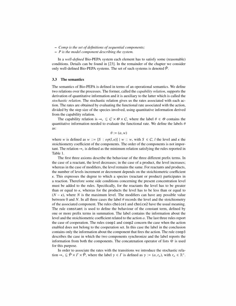
3.3 The semantics

The semantics of Bio-PEPA is defined in terms of an operational semantics. We definetwo relations over the processes. The former, called the capability relation, supports thederivation of quantitative information and it is auxiliary to the latter which is called thestochastic relation. The stochastic relation gives us the rates associated with each ac-tion. The rates are obtained by evaluating the functional rate associated with the action,divided by the step size of the species involved, using quantitative information derivedfrom the capability relation.

The capability relation is −→c ⊆ C × Θ × C, where the label θ ∈ Θ contains thequantitative information needed to evaluate the functional rate. We define the labels θas:

θ := (α,w)

where w is defined as w ::= [S : op(l, κ)] | w :: w, with S ∈ C, l the level and κ thestoichiometry coefficient of the components. The order of the components is not impor-tant. The relation −→c is defined as the minimum relation satisfying the rules reported inTable 1.

The first three axioms describe the behaviour of the three different prefix terms. Inthe case of a reactant, the level decreases; in the case of a product, the level increases;whereas in the case of modifiers, the level remains the same. For reactants and products,the number of levels increment or decrement depends on the stoichiometric coefficientκ. This expresses the degree to which a species (reactant or product) participates ina reaction. Therefore some side conditions concerning the present concentration levelmust be added to the rules. Specifically, for the reactants the level has to be greaterthan or equal to κ, whereas for the products the level has to be less than or equal to(N − κ), where N is the maximum level. The modifiers can have any possible valuebetween 0 and N. In all three cases the label θ records the level and the stoichiometryof the associated component. The rules choice1 and choice2 have the usual meaning.The rule constant is used to define the behaviour of the constant term, defined byone or more prefix terms in summation. The label contains the information about thelevel and the stoichiometric coefficient related to the action α. The last three rules reportthe case of cooperation. The rules coop1 and coop2 concern the case when the actionenabled does not belong to the cooperation set. In this case the label in the conclusioncontains only the information about the component that fires the action. The rule coop3describes the case in which the two components synchronize and the label reports theinformation from both the components. The concatenation operator of lists @ is usedfor this purpose.

In order to associate the rates with the transitions we introduce the stochastic rela-tion −→s ⊆ P × Γ × P, where the label γ ∈ Γ is defined as γ := (α, rα), with rα ∈ R+.

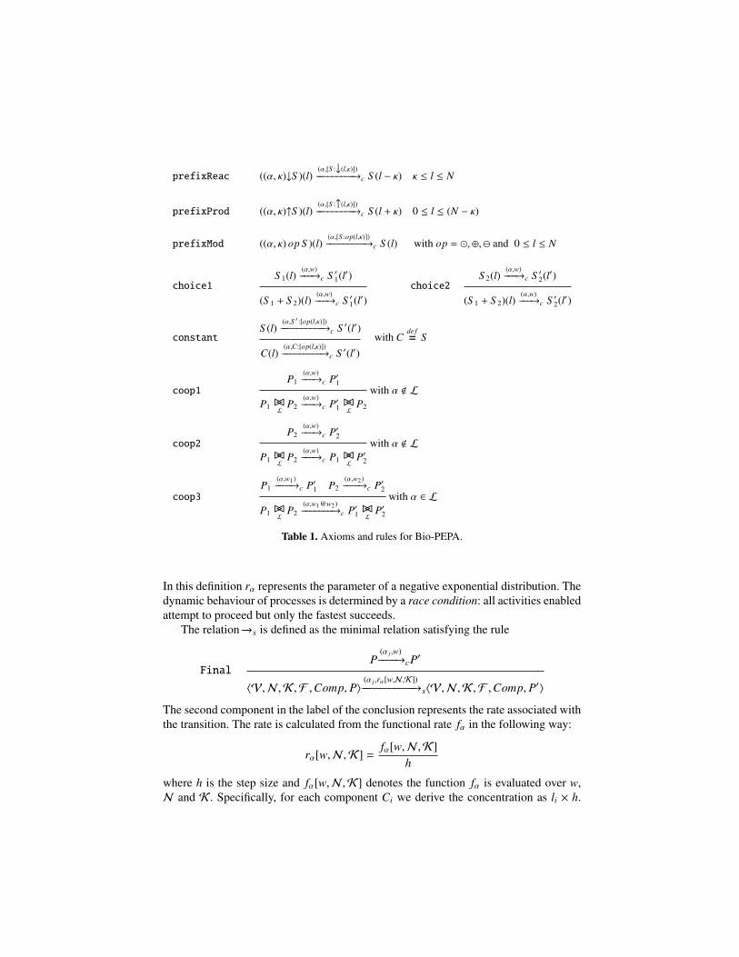
prefixReac ((α, κ)↓S )(l)(α,[S :↓(l,κ)])−−−−−−−−−→c S (l − κ) κ ≤ l ≤ N

prefixProd ((α, κ)↑S )(l)(α,[S :↑(l,κ)])−−−−−−−−−→c S (l + κ) 0 ≤ l ≤ (N − κ)

prefixMod ((α, κ) op S )(l)(α,[S :op(l,κ)])−−−−−−−−−→c S (l) with op = �,⊕, and 0 ≤ l ≤ N

choice1S 1(l)

(α,w)−−−→c S ′1(l′)

(S 1 + S 2)(l)(α,w)−−−→c S ′1(l′)

choice2S 2(l)

(α,w)−−−→c S ′2(l′)

(S 1 + S 2)(l)(α,w)−−−→c S ′2(l′)

constantS (l)

(α,S ′:[op(l,κ)])−−−−−−−−−−→c S ′(l′)

C(l)(α,C:[op(l,κ)])−−−−−−−−−→c S ′(l′)

with Cde f= S

coop1P1

(α,w)−−−→c P′1

P1 BCL

P2(α,w)−−−→c P′1 BCL P2

with α < L

coop2P2

(α,w)−−−→c P′2

P1 BCL

P2(α,w)−−−→c P1 BC

LP′2

with α < L

coop3P1

(α,w1)−−−−→c P′1 P2

(α,w2)−−−−→c P′2

P1 BCL

P2(α,w1@w2)−−−−−−−→c P′1 BCL P′2

with α ∈ L

Table 1. Axioms and rules for Bio-PEPA.

In this definition rα represents the parameter of a negative exponential distribution. Thedynamic behaviour of processes is determined by a race condition: all activities enabledattempt to proceed but only the fastest succeeds.

The relation −→s is defined as the minimal relation satisfying the rule

FinalP

(α j,w)−−−−→cP′

〈V,N ,K ,F ,Comp, P〉(α j,rα[w,N ,K])−−−−−−−−−−−→s〈V,N ,K ,F ,Comp, P′〉

The second component in the label of the conclusion represents the rate associated withthe transition. The rate is calculated from the functional rate fα in the following way:

rα[w,N ,K] =fα[w,N ,K]

h

where h is the step size and fα[w,N ,K] denotes the function fα is evaluated over w,N and K . Specifically, for each component Ci we derive the concentration as li × h.

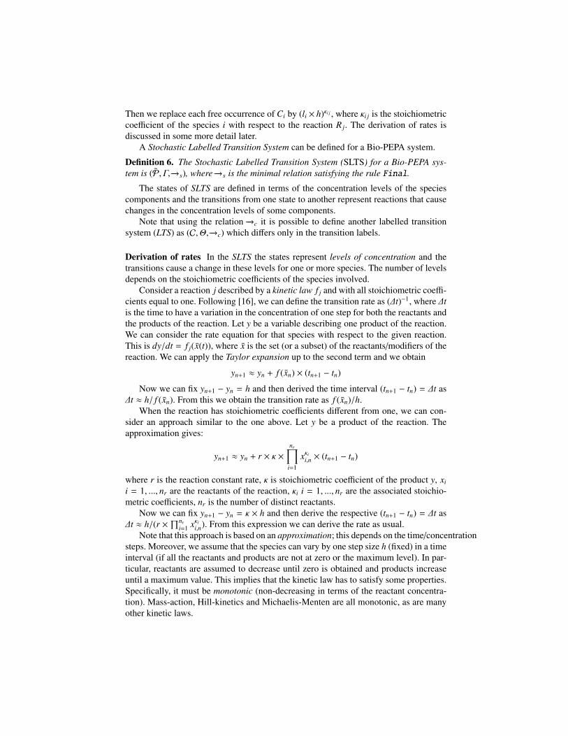
Then we replace each free occurrence of Ci by (li × h)κi j , where κi j is the stoichiometriccoefficient of the species i with respect to the reaction R j. The derivation of rates isdiscussed in some more detail later.

A Stochastic Labelled Transition System can be defined for a Bio-PEPA system.

Definition 6. The Stochastic Labelled Transition System (SLTS) for a Bio-PEPA sys-tem is (P, Γ,−→s), where −→s is the minimal relation satisfying the rule Final.

The states of SLTS are defined in terms of the concentration levels of the speciescomponents and the transitions from one state to another represent reactions that causechanges in the concentration levels of some components.

Note that using the relation −→c it is possible to define another labelled transitionsystem (LTS) as (C, Θ,−→c) which differs only in the transition labels.

Derivation of rates In the SLTS the states represent levels of concentration and thetransitions cause a change in these levels for one or more species. The number of levelsdepends on the stoichiometric coefficients of the species involved.

Consider a reaction j described by a kinetic law f j and with all stoichiometric coeffi-cients equal to one. Following [16], we can define the transition rate as (∆t)−1, where ∆tis the time to have a variation in the concentration of one step for both the reactants andthe products of the reaction. Let y be a variable describing one product of the reaction.We can consider the rate equation for that species with respect to the given reaction.This is dy/dt = f j(x(t)), where x is the set (or a subset) of the reactants/modifiers of thereaction. We can apply the Taylor expansion up to the second term and we obtain

yn+1 ≈ yn + f (xn) × (tn+1 − tn)

Now we can fix yn+1 − yn = h and then derived the time interval (tn+1 − tn) = ∆t as∆t ≈ h/ f (xn). From this we obtain the transition rate as f (xn)/h.

When the reaction has stoichiometric coefficients different from one, we can con-sider an approach similar to the one above. Let y be a product of the reaction. Theapproximation gives:

yn+1 ≈ yn + r × κ ×nr∏

i=1

xκii,n × (tn+1 − tn)

where r is the reaction constant rate, κ is stoichiometric coefficient of the product y, xi

i = 1, ..., nr are the reactants of the reaction, κi i = 1, ..., nr are the associated stoichio-metric coefficients, nr is the number of distinct reactants.

Now we can fix yn+1 − yn = κ × h and then derive the respective (tn+1 − tn) = ∆t as∆t ≈ h/(r ×

∏nri=1 xκii,n). From this expression we can derive the rate as usual.

Note that this approach is based on an approximation; this depends on the time/concentrationsteps. Moreover, we assume that the species can vary by one step size h (fixed) in a timeinterval (if all the reactants and products are not at zero or the maximum level). In par-ticular, reactants are assumed to decrease until zero is obtained and products increaseuntil a maximum value. This implies that the kinetic law has to satisfy some properties.Specifically, it must be monotonic (non-decreasing in terms of the reactant concentra-tion). Mass-action, Hill-kinetics and Michaelis-Menten are all monotonic, as are manyother kinetic laws.

From biochemical networks to Bio-PEPA We define a translation, tr BM BP, froma biochemical networkM to a Bio-PEPA system P = 〈V,N ,K ,FR,Comp, P〉, basedon the following abstraction:

1. Each compartment is defined in the set V in terms of a name and an associatedvolume. Recall that currently in Bio-PEPA, compartments are not involved activelyin the reactions and therefore are not represented by processes.

2. Each species i in the network is described by a species component Ci ∈ Comp. Theconstant component Ci is defined by the “sum” of elementary components describ-ing the interaction capabilities of the species. We suppose that there is at most oneterm in each species component with an action of type α. A single definition canexpress the behaviour of the species at any level.

3. Each reaction j is associated with an action type α j and its dynamics is describedby a specific function fα j ∈ FR. The constant parameters used in the function canbe defined in K .

4. The model P is defined as the cooperation of the different components Ci.

3.4 Some examples

Now we present some simple examples in order to show how Bio-PEPA can be used tocapture some biological situations.

Example 1: Mass-action kinetics Consider the reaction 2X + Y; fM−−−→3Z, described by

the mass-action kinetic law fM = r × X2 × Y . The three species can be specified by thesyntax:

Xdef= (α, 2)↓X Y

def= (α, 1)↓Y Z

def= (α, 3)↑Z

The system is described by (X(lX0) BC{α}

Y(lY0)) BC{α}

Z(lZ0), where lX0, lY0 and lZ0 denote theinitial concentration level of the three components. The functional rate is fα = f MA(r).The rate associated with a transition is given by:

rα =r × (lX × h)2 × (lY × h)

h

where lX , lY are the concentration levels for the species X and Y in a given state and h isthe step size of all the species. The reaction can happen only if we have at least 3 levels(0, 1, 2) for X and 4 levels (0, 1, 2, 3) for Z.

Example 2: Michaelis-Menten kinetics One of the most commonly used kinetic lawsis Michaelis-Menten. It describes a basic enzymatic reaction from the substrate S to the

product P and is written as SE; fE−−−→P, where E is the enzyme involved in the reaction.

This reaction is an approximation of a sequence of two reactions, under the quasi-steadystate assumption (QSSA). The whole sequence of reactions is described by the kineticlaw fE =

vM×E×S(KM+S ) . For more details about the derivation of this kinetic law and the

meaning of parameters see [65].

The three species can be specified in Bio-PEPA by the following components:

Sdef= (α, 1)↓S P

def= (α, 1)↑P E

def= (α, 1) ⊕ E

The system is described by (S (lS 0) BC{α}

E(lE0)) BC{α}

P(lP0) and the functional rate isfα = f MM(vM ,KM).

The transition rate is given by:

rα =vM × (lS × h) × (lE × h)

(KM + lS × h)×

1h

where lS , lE are the concentration levels for the species S and E in a given state and h isthe step size of all the species. The reaction can happen only if we have at least 3 levels(0, 1, 2) for all the species involved.

Example 3: competitive inhibition Competitive inhibition is a form of enzyme inhibi-tion where binding of the inhibitor to the enzyme prevents binding of the substrate andvice versa. In classical competitive inhibition, the inhibitor binds to the same active siteas the normal enzyme substrate, without undergoing a reaction. The substrate moleculecannot enter the active site while the inhibitor is there, and the inhibitor cannot enterthe site when the substrate is there. This reaction is described as:

S + E + I ←→ SE −→ P + El

EI

where S is the substrate, E the enzyme, I the inhibitor and P the product. Under QSSAthe intermediate species SE and EI are constant and we can approximate the reactions

above by a unique reaction SE,I: fI−−−−→P, with rate fI =

vc × S × ES + KM(1 + I

KI), where vc is the

the turnover number (catalytic constant), KM is the Michaelis-constant and KI is theinhibition constant.

The specification in Bio-PEPA is:

Sdef= (α, 1)↓S P

def= (α, 1)↑P E

def= (α, 1) ⊕ E I

def= (α, 1) I

The system is described by ((S (lS 0) BC{α}

E(lE0)) BC{α}

I(lI0)) BC{α}

P(lP0) with functional rate

fα = fCI((vc,KM ,KI), S , E, I) =vc × S × E

S + KM(1 + IKI

).

The transition rate is given by:

rα =vc × (lS × h) × (lE × h)

(lS × h + KM(1 + lI×hKI

))×

1h

where lS , lE , lI are the concentration levels for the species S , E, I in a given state andh is the step size of all the species. The reaction can happen only if we have at least 3levels (0, 1, 2) for all the species involved.

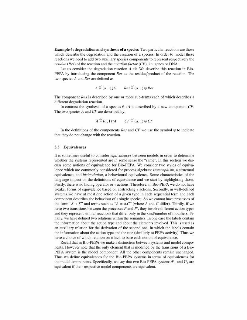
Example 4: degradation and synthesis of a species Two particular reactions are thosewhich describe the degradation and the creation of a species. In order to model thesereactions we need to add two auxiliary species components to represent respectively theresidue (Res) of the reaction and the creation factor (CF), i.e. genes or DNA.

Let us consider the degradation reaction A−→∅. We describe this reaction in Bio-PEPA by introducing the component Res as the residue/product of the reaction. Thetwo species A and Res are defined as:

Adef= (α, 1)↓A Res

def= (α, 1) � Res

The component Res is described by one or more sub-terms each of which describes adifferent degradation reaction.

In contrast the synthesis of a species ∅−→A is described by a new component CF.The two species A and CF are described by:

Adef= (α, 1)↑A CF

def= (α, 1) � CF

In the definitions of the components Res and CF we use the symbol � to indicatethat they do not change with the reaction.

3.5 Equivalences

It is sometimes useful to consider equivalences between models in order to determinewhether the systems represented are in some sense the “same”. In this section we dis-cuss some notions of equivalence for Bio-PEPA. We consider two styles of equiva-lence which are commonly considered for process algebras: isomorphism, a structuralequivalence, and bisimulation, a behavioural equivalence. Some characteristics of thelanguage impact on the definitions of equivalence and we start by highlighting those.Firstly, there is no hiding operator or τ actions. Therefore, in Bio-PEPA we do not haveweaker forms of equivalence based on abstracting τ actions. Secondly, in well-definedsystems we have at most one action of a given type in each sequential term and eachcomponent describes the behaviour of a single species. So we cannot have processes ofthe form “S + S ” and terms such as “A = a.C” (where A and C differ). Thirdly, if wehave two transitions between the processes P and P′, they involve different action typesand they represent similar reactions that differ only in the kind/number of modifiers. Fi-nally, we have defined two relations within the semantics. In one case the labels containthe information about the action type and about the elements involved. This is used asan auxiliary relation for the derivation of the second one, in which the labels containthe information about the action type and the rate (similarly to PEPA activity). Thus wehave a choice of which relation on which to base each notion of equivalence.

Recall that in Bio-PEPA we make a distinction between systems and model compo-nents. However note that the only element that is modified by the transitions of a Bio-PEPA system is the model component. All the other components remain unchanged.Thus we define equivalences for the Bio-PEPA systems in terms of equivalences forthe model components. Specifically, we say that two Bio-PEPA systems P1 and P2 areequivalent if their respective model components are equivalent.

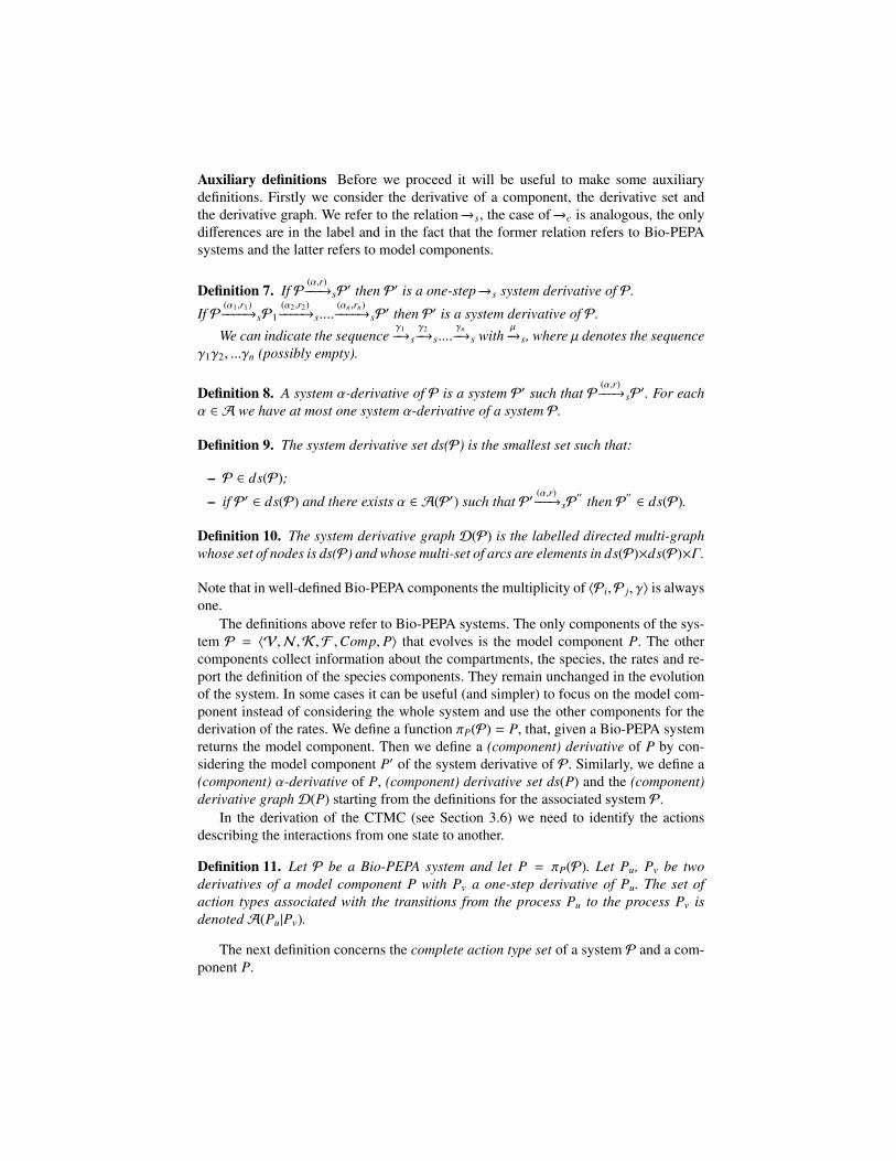
Auxiliary definitions Before we proceed it will be useful to make some auxiliarydefinitions. Firstly we consider the derivative of a component, the derivative set andthe derivative graph. We refer to the relation −→s, the case of −→c is analogous, the onlydifferences are in the label and in the fact that the former relation refers to Bio-PEPAsystems and the latter refers to model components.

Definition 7. If P(α,r)−−−→sP

′ then P′ is a one-step −→s system derivative of P.

If P(α1,r1)−−−−→sP1

(α2,r2)−−−−→s....

(αn,rn)−−−−→sP

′ then P′ is a system derivative of P.

We can indicate the sequenceγ1−→s

γ2−→s....

γn−→s with

µ−→s, where µ denotes the sequence

γ1γ2, ...γn (possibly empty).

Definition 8. A system α-derivative of P is a system P′ such that P(α,r)−−−→sP

′. For eachα ∈ A we have at most one system α-derivative of a system P.

Definition 9. The system derivative set ds(P) is the smallest set such that:

– P ∈ ds(P);

– if P′ ∈ ds(P) and there exists α ∈ A(P′) such that P′(α,r)−−−→sP

′′

then P′′

∈ ds(P).

Definition 10. The system derivative graph D(P) is the labelled directed multi-graphwhose set of nodes is ds(P) and whose multi-set of arcs are elements in ds(P)×ds(P)×Γ.

Note that in well-defined Bio-PEPA components the multiplicity of 〈Pi,P j, γ〉 is alwaysone.

The definitions above refer to Bio-PEPA systems. The only components of the sys-tem P = 〈V,N ,K ,F ,Comp, P〉 that evolves is the model component P. The othercomponents collect information about the compartments, the species, the rates and re-port the definition of the species components. They remain unchanged in the evolutionof the system. In some cases it can be useful (and simpler) to focus on the model com-ponent instead of considering the whole system and use the other components for thederivation of the rates. We define a function πP(P) = P, that, given a Bio-PEPA systemreturns the model component. Then we define a (component) derivative of P by con-sidering the model component P′ of the system derivative of P. Similarly, we define a(component) α-derivative of P, (component) derivative set ds(P) and the (component)derivative graphD(P) starting from the definitions for the associated system P.

In the derivation of the CTMC (see Section 3.6) we need to identify the actionsdescribing the interactions from one state to another.

Definition 11. Let P be a Bio-PEPA system and let P = πP(P). Let Pu, Pv be twoderivatives of a model component P with Pv a one-step derivative of Pu. The set ofaction types associated with the transitions from the process Pu to the process Pv isdenotedA(Pu|Pv).

The next definition concerns the complete action type set of a system P and a com-ponent P.

Definition 12. The complete action type set of a system P is defined as:

A = ∪Pi∈ds(P)A(Pi)

The complete action type set of a component P is defined similarly.

Other useful definitions are the ones concerning the exit rate and transition rates. Inthe following we report the definition for the model components, but a similar definitioncan be used for Bio-PEPA systems.

Definition 13. Let us consider a Bio-PEPA system P = 〈V,N ,K ,F ,Comp, P〉 and letP1, P2 ∈ ds(P). The exit rate of a process P1 is defined as:

rate(P1) =∑

{α|∃P2.P1

(α,rα[w,N ,K])−−−−−−−−−−→sP2, P1=πP(P1)}

rα[w,N ,K]

Similarly, the transition rate is defined as:

rate(P1 | P2) =∑

{α|P1

(α,rα[w,N ,K])−−−−−−−−−−→sP2, P1=πP(P1), P2=πP(P2)}

rα[w,N ,K]

For the label γ in the stochastic relation, the function action(γ) = α extracts the firstcomponent of the pair (i.e. the action type) and the function rate(γ) = r ∈ R returns thesecond component (i.e. the rate).

In the following we use the same symbol to denote equivalences for both the systemand the corresponding model component. In this section we present definitions of iso-morphism and strong bisimulation which are similar to the relations defined for PEPAin [42]. Furthermore we show some relationships between the defined equivalences.

Isomorphism Isomorphism is a strong notion of equivalence based on the derivationgraph of the components (systems). Broadly speaking, two components (systems) areisomorphic if they generate derivation graphs with the same structure and capable ofcarrying out exactly the same activities.

We have the following definition of isomorphism based on the capability relation:

Definition 14. Let P1, P2 be two Bio-PEPA systems whose model components areP and Q, respectively. A function F : ds(P) → ds(Q) is a component isomorphismbetween P and Q, with respect to −→c, ifF is an injective function and for any componentP′ ∈ ds(P), A(P′) = A(F (P′)), with rα[P′,N ,K] = r′α[F (P′),N ′,K ′] for each α ∈A(P), and for all α ∈ A the set of α-derivatives of F (P′) is the same as the set ofF−images of the α-derivatives of P′, with respect to −→c.

This is a very strong relation because the labels associated with the capability rela-tion contain a lot of information, all of which must be matched. Formally, we can defineisomorphic components in the following way:

Definition 15. Let P1, P2 be two Bio-PEPA systems whose model components are Pand Q. P and Q are isomorphic with respect to −→c (denoted P =c Q), if there exists acomponent isomorphismF between them such thatD(F (P)) = D(Q), whereD denotesthe derivative graph.

We can now define when two Bio-PEPA systems are isomorphic.

Definition 16. Let P1, P2 be two Bio-PEPA systems whose model components are Pand Q. P1 and P2 are isomorphic with respect to −→c (denoted P1 =c P2), if P =c Q.

A similar structural relation based on the stochastic relation can also be definedand used to characterise another form of isomorphism between systems (components)=s (see [?] for details). Both isomorphisms, =c and =s are equivalence relations, andcongruences with respect to the combinators of Bio-PEPA. In both cases they retainenough information about the structure and behaviour of the isomorphic componentsto ensure that they give rise to identical underlying Markov processes. However, =c ismore strict than =s, i.e. there will be pairs of systems (components) which satisfy =s

but do not satisfy =c.

Equational laws Once an equivalence relation has been defined it can be used to estab-lish equational laws which may be used to manipulate models and recognise equivalentterms. In the following the symbol “=” denotes either =c or =s. The proof of the lawsfollow from the definition of isomorphism and the semantic rules.

Choice1) (P + Q) BC

LS = (Q + P) BC

LS

2) (P + (Q + R)) BCL

S = ((P + Q) + R) BCL

SCooperation

1. P BCL

Q = Q BCL

P

2. P BCL

(Q BCL

R) = (P BCL

Q) BCL

R

3. P BCK

Q = P BCL

Q if K ∩ (A(P) ∪ A(Q)) = L

4. (P BCL

Q) BCK

R ={

P BCL

(Q BCK

R) if A(R) ∩ (L\K) = ∅ ∧ A(P) ∩ (K\L) = ∅Q BC

L(P BC

KR) if A(R) ∩ (L\K) = ∅ ∧ A(Q) ∩ (K\L) = ∅

Constant If Adef= P then A = P

Bio-PEPA systemsLet P1 and P2 be two Bio-PEPA systems, with P = πP(P1) and Q = πP(P2).If P = Q then P1 = P2.

Strong bisimulation The definition of bisimulation is based on the labelled transitionsystem. Strong bisimulation captures the idea that bisimilar components (systems) areable to perform the same actions with same rates resulting in derivatives that are them-selves bisimilar. This makes the components (systems) indistinguishable to an externalobserver. As with isomorphism we can develop two definition based on the two seman-tic relations. This time for illustration we present the definitions based on the stochasticrelation. The strong capability bisimulation, ∼c, is defined similarly (see [?] for details).

Definition 17. A binary relation R ⊆ P × P is a strong stochastic bisimulation, if(P1,P2) ∈ R implies for all α ∈ A:

– if P1γ1−→sP

′1 then, for some P′2 and γ2, P2

γ2−→sP

′2 with (P′1,P′2) ∈ R and

1. action(γ1) = action(γ2) = α2. rate(γ1) = rate(γ2)

– the symmetric definition with P2 replacing P1.

Definition 18. Let P1, P2 be two Bio-PEPA systems whose model components areP and Q, respectively. P and Q are strong stochastic bisimilar, written P ∼s Q, if(P1,P2) ∈ R for some strong stochastic bisimulation R.

Definition 19. Let P1, P2 be two Bio-PEPA systems whose model components are Pand Q, respectively.P1, P2 are strong stochastic bisimilar, writtenP1 ∼s P2, if P ∼s Q.

Both ∼c and ∼s are equivalence relations and congruences with respect to the com-binators of Bio-PEPA. Moreover it is straightforward to see that isomorphism impliesstrong bisimulation in both cases.

Example Consider the following systems representing two biological systems. Theformer system P1 represents a system described by an enzymatic reaction with kinetic

lawv1 × E × S

K1 + S, where S is the substrate and E the enzyme. We have that the set N is

defined as “S : h,NS ; P : h,NP; E : 1, 1; ” for some step size h and maximum levelsNS and NP. The component and the model components are defined as:

Sdef= (α, 1)↓S E

def= (α, 1) ⊕ E P

def= (α, 1)↑P

The model component P1 is (S (lS 0) BC{α}

E(1)) BC{α}

P(lP0). The functional rate is fα =f MM(v1,K1).

The second system P2 describes an enzymatic reaction where the enzyme is left

implicit (it is constant). The rate is given byv1 × S ′

K1 + S ′, where S ′ is the substrate.

We have that the set N is defined as “S ′ : h,NS ′ ; P′ : h,NP′ ; ”.The components are defined as S′

def= (α, 1)↓S ′ and P′

def= (α, 1)↑P′ and the model

component P2 is S ′(lS 0) BC{α}

P′(lP0). In this case fα = f MM′((v1,K1), S ′) =v1 × S ′

K1 + S ′and

the component S ′ and P′ have the same number of levels/maximum concentration of Sand P.

We have that P1 ∼s P2, but P1 /c P2, because the number of enzymes is differ-ent. The same relations are valid if the systems rather than the model components areconsidered.

3.6 Analysis

A Bio-PEPA system is an intermediate, formal, compositional representation of the bi-ological model. Based on this representation we can perform different kinds of analysis.In this section we discuss briefly how to use a Bio-PEPA system to derive a CTMC withlevels, a set of Ordinary Differential Equations (ODEs), a Gillespie simulation and aPRISM model.

From Bio-PEPA to CTMC As for the reagent-centric view of PEPA, the CTMC as-sociated with the system refers to the concentration levels of the species components.Specifically, the states of the CTMC are defined in terms of concentration levels and thetransitions from one state to the other describe some variations in these levels. Hereafterwe call the CTMC derived from a Bio-PEPA system (or from a PEPA reagent-centricview system) CTMC with levels.

Theorem 1. For any finite Bio-PEPA system P = 〈V,N ,K ,FR,Comp, P〉, if we definethe stochastic process X(t) such that X(t) = Pi indicates that the system behaves as thecomponent Pi at time t, then X(t) is a Markov Process.

The proof is not reproduced here but it is analogous the one presented for PEPA [42].Instead of the PEPA activity we consider the label γ and the rate is obtained by evaluat-ing the functional rate in the system. We consider finite models to ensure that a solutionfor the CTMC is feasible. This is equivalent to supposing that each species in the modelhas a maximum level of concentration.

Theorem 2. Given (P, Γ,−→s), let P be a Bio-PEPA system, with model component P.Let nc = |ds(P)|, where ds(P) is the derivative set of P. Then the infinitesimal generatormatrix of the CTMC for P is a square matrix Q (nc×nc) whose elements qu,v are definedas

qu,v =∑

α j∈A(Pu |Pv)

rα j [wu,N ,K] if u , v qu,u = −∑u,v

qu,v otherwise.

where Pu, Pv are two derivatives of P.

It is worth noting that the states of CTMC are defined in terms of the derivatives ofthe model component. These derivatives are uniquely identified by the levels of speciescomponents in the system, so we can give the following definition of CTMC states:

Definition 20. The CTMC states derived from a Bio-PEPA system can be defined asvectors of levels σ = (l1, l2, ..., ln), where li , for i = 1, 2, ..., n is the level of the speciesi and n is the total number of species. We can avoid consideration of the two levels forRes and CF as they are always constant.

This leads to the following proposition.

Proposition 1. Let P be a Bio-PEPA system with model component P. Let Pu and Pv

be two derivatives of P such that the latter is one-step derivative of the former. If thereexist two action types α1 and α2 that belong toA(Pu|Pv) then:

1. α1 , α2;2. the two action types refer to two transitions/biological reactions that differ only in

the modifiers.

If two transitions are possible between a pair of states, the actions involved are differ-ent and they represent reactions that differ only in the modifiers and/or the number ofenzymes used. The former point follows from the definition of well-defined Bio-PEPAsystem. The second point follows because the only possibility to have two transitionsbetween two given states is that the associated reactions have the same reactants andproducts. We can see this by observing that the states depend on the levels and the reac-tions cause some changes in these levels. The only elements that do not change duringa reaction are the modifiers.

From Bio-PEPA to ODEs The translation into ODEs is similar to the method proposedfor PEPA (reagent-centric view) [13]. It is based on the syntactic presentation of themodel and on the derivation of the stoichiometry matrix D = {di j} from the definitionof the components. The entries of the matrix are the stoichiometric coefficients of thereactions and are obtained in the following way: for each component Ci consider theprefix subterms Ci j representing the contribution of the species i to the reaction j. If theterm represents a reactant we write the corresponding stoichiometry κi j as −κi j in theentry di j. For a product we write +κi j in the entry di j. All other cases are null.

The derivation of ODEs from the Bio-PEPA systemP, hereafer called tODE , is basedon the following steps:

1. definition of the stoichiometry (n × m) matrix D, where n is the number of speciesand m is the number of molecules;

2. definition of the kinetic law vector (m × 1) vKL containing the kinetic laws of eachreaction;

3. association of the variable xi with each component Ci and definition of the vector(n × 1) x.

The ODE system is then obtained as:

dxdt= D × vKL

with initial concentrations xi0 = li0 × h, for i = 1, ..., n.The following property holds:

Property 1. For a biochemical networkM and a Bio-PEPA system P= tr BM BP(M),we have that tODE(P) = tBODE(M), where tODE and tBODE are the translation functionsfrom Bio-PEPA and the biological system into ODEs, respectively.

The ODE system derived from a Bio-PEPA system P is “equal” to the one obtaineddirectly from the biological network itself. This means that in the translation into Bio-PEPA no information for the derivation of ODEs is lost. This result follows from thefact that in both cases we derive the stoichiometric matrix and, for construction, theyare the same in both cases. However the Bio-PEPA model can collect generally moreinformation than the respective ODEs. We have this further result:

Property 2. Given two biochemical networksM1 andM2 we define the correspondingBio-PEPA models P1 = tr BM BP(M1) and P2 = tr BM BP(M2). Let tODE(P1) andtODE(P2) be the two ODE systems obtained from P1 and P2 respectively. If tODE(P1) =tODE(P2) it does not imply that P1 is “equivalent” to P2.

The above result can be easily seen with appropriate counterexamples. For exampleconsider the Bio-PEPA models corresponding to the following sets of reactions: {A

r−→B+

C; Ar−→B; A

r−→C + D} and {A

2r−→B + C; A

r−→D}. The two Bio-PEPA models are different,

but the ODE systems that we derived from them coincide.

From Bio-PEPA to stochastic simulation Gillespie’s stochastic simulation algorithm[36] is a widely-used method for the simulation of biochemical reactions. It deals withhomogenous, well-stirred systems in thermal equilibrium and constant volume, com-posed of n different species that interact through m reactions. Broadly speaking, thegoal is to describe the evolution the system X(t), described in terms of the number ofelements of each species, starting from an initial state. Every reaction is characterizedby a stochastic rate constant c j, termed the basal rate (derived from the constant rater by means of some simple relations proposed in [36, 68]). Using this it is possible tocalculate the actual rate a j(X(t)) of the reaction, that is the probability of the reactionR j occurring in time (t, t + ∆t) given that the system is in a specific state.

The algorithm is based essentially on the following two steps:

– calculation of the next reaction that occurs in the system;– calculation of the time when the next reaction occurs.

We derive the information above from two conditional density functions:p( j | X(t)) = a j(X(t))/a0, that is, the probability that the next reaction is R j andp(τ|X(t)) = a0ea0X(t)τ, the probability that the next reaction occurs in [t + τ, t + τ + dτ],

where a0 =m∑

v=1av(X(t)).

The translation of a Bio-PEPA model to a Gillespie’s simulation is similar to theapproach proposed for ODEs. The main drawbacks are the definition of the rates andthe correctness of the approach in the case of general kinetic laws. Indeed Gillespie’sstochastic simulation algorithm supposes elementary reactions and constant rates (mass-action kinetics). If the model contains only this kind of reactions the translation isstraightforward. If there are non-elementary reactions and general kinetic laws, it isa widely-used approach to consider them translated directly into a stochastic context.This is not always valid and some counterexamples have been demonstrated [11]. Theauthors of [11] showed that when Gillespie’s algorithm is applied to Hill kinetics in thecontext of the transcription initiation of autoregulated genes, the magnitude of fluctu-ations is overestimated. The application of Gillespie’s algorithm in the case of generalkinetics laws is discussed by several authors [1, 17]. Rao and Arkin [1] show that thisapproach is valid in the case of some specific kinetic laws, such as Michaelis-Mentenand inhibition. However, it is important to remember that these laws are approxima-tions, based on some assumptions that specific conditions (such as “S � E” in thecase of Michaelis-Menten) hold. The approach followed here is as in [47]: we apply

Gillespie’s algorithm, but particular attention must be paid to the interpretation of thesimulation results and to their validity.

The definition of a Gillespie model is based on:

– definition of the state vector X. It is composed of n components Xi, representing thenumber of elements for each species i.

– Definition of the initial condition X0. The values are given by:

Xi0 = li0 × h × NA × vi molecules

where NA is the Avogadro’s number that indicates the number of molecules in amole of a substance and vi is the volume size of the containing compartment Vi.

– Definition of the actual rate for each reaction. We have two cases:1. reactions whose dynamics is described by mass-action law and with constant

rate r j. The actual rate for the reaction is:

a j(X j) = c j × fh(X j)

where c j is the stochastic rate constant, fh is a function that gives the numberof distinct combinations of reactant molecules and X j are the species involvedin the reaction j. The stochastic rate constant is defined in [68] as:

c j =r j

(NA × v)ntot−1 ×

n j∏u=1

κu j!

where n j is the number of distinct reactants in the reaction j, r j is the rate of

the reaction and ntot =

n j∑u=1

κu j is the total number of reactants 6.

Finally, the number of possible combinations of reactants is defined as

fh((X j) =n j∏

u=1

(Xp(u, j)

κu j

)∼

n j∏u=1

(Xp(u, j))κu j

n j∏u=1

κu j!

2. reactions with general kinetic laws fα j (k, C). The actual rate is:

a j(X j) = fα j (k, X j)

From Bio-PEPA to PRISM PRISM [61] is a probabilistic model checker, a tool forthe formal modelling and analysis of systems which exhibit random or probabilistic be-haviour. PRISM has been used to analyse systems from a wide range of application do-mains. Models are described using the PRISM language, a simple state-based language

6 We assume that all the species that are involved in the reaction as reactants are inside the samecompartment with volume v.

and it is possible to specify quantitative properties of the system using a temporal logic,called CSL [2] (Continuous Stochatic Logic). For our purposes the underlying mathe-matical model of a PRISM model is a CTMC and the PRISM models we generate fromBio-PEPA correspond to the CTMCs with levels. However we present the translationseparately as the models are specified in the PRISM language.

The PRISM language is composed of modules and variables. A model is composedof a number of modules which can interact with each other. A module contains a numberof local variables. The values of these variables at any given time constitute the state ofthe module. The global state of the whole model is determined by the local state of allmodules. The behaviour of each module is described by a set of commands. Each updatedescribes a transition which the module can make if the guard is true. A transition isspecified by giving the new values of the variables in the module, possibly as a functionof other variables. Each update is also assigned a probability (or in some cases a rate)which will be assigned to the corresponding transition. It is straightforward to translatea Bio-PEPA system into a PRISM model. We have the following correspondences:

– The model is defined as stochastic (this term is used in PRISM for CTMC).– Each element in the set of parameters K is defined as a global constant.– The maximum levels, the concentration steps and the volume sizes are defined as

global constants.– Each species component is represented by a PRISM module. The species compo-

nent concentration is represented by a local variable and it can (generally) assumevalues between 0 and Ni. For each sub-term (i.e. reaction where the species is in-volved) we have a definition of a command. The name of the command is relatedto the action α (and then to the associated reaction). The guards and the changein levels are defined according to whether the element is a reactant, a product or amodifier of the reactions.

– The functional rates are defined inside an auxiliary module.– In PRISM the rate associated with an action is the product of the rates of the com-

mands in the different modules that cooperate. For each reaction, we give the value“1” to the rate of each command involved in the reaction, with the exception of thecommand in the module containing the functional rates. In this case the rate is thefunctional rate f , expressing the kinetic law. The rate associated with a reaction isgiven by 1 × 1 × ... × f = f , as desired.

4 Examples

This section reports the translation of three biological models into Bio-PEPA and someanalysis results. The first example is taken from [37] and describes a minimal modelfor the cascade of post-translational modifications that modulate the activity of cdc2kinase during the cell cycle. The second model is taken from [11] and concerns a simplegenetic network with negative feedback loop. The last example is the repressilator [33],a synthetic genetic network with an oscillating behaviour.

In the present work the stochastic and deterministic simulations are obtained export-ing the Bio-PEPA system by means of the maps described in Section 3.6. An automatictranslation is under implementation.

4.1 The Goldbeter’s model

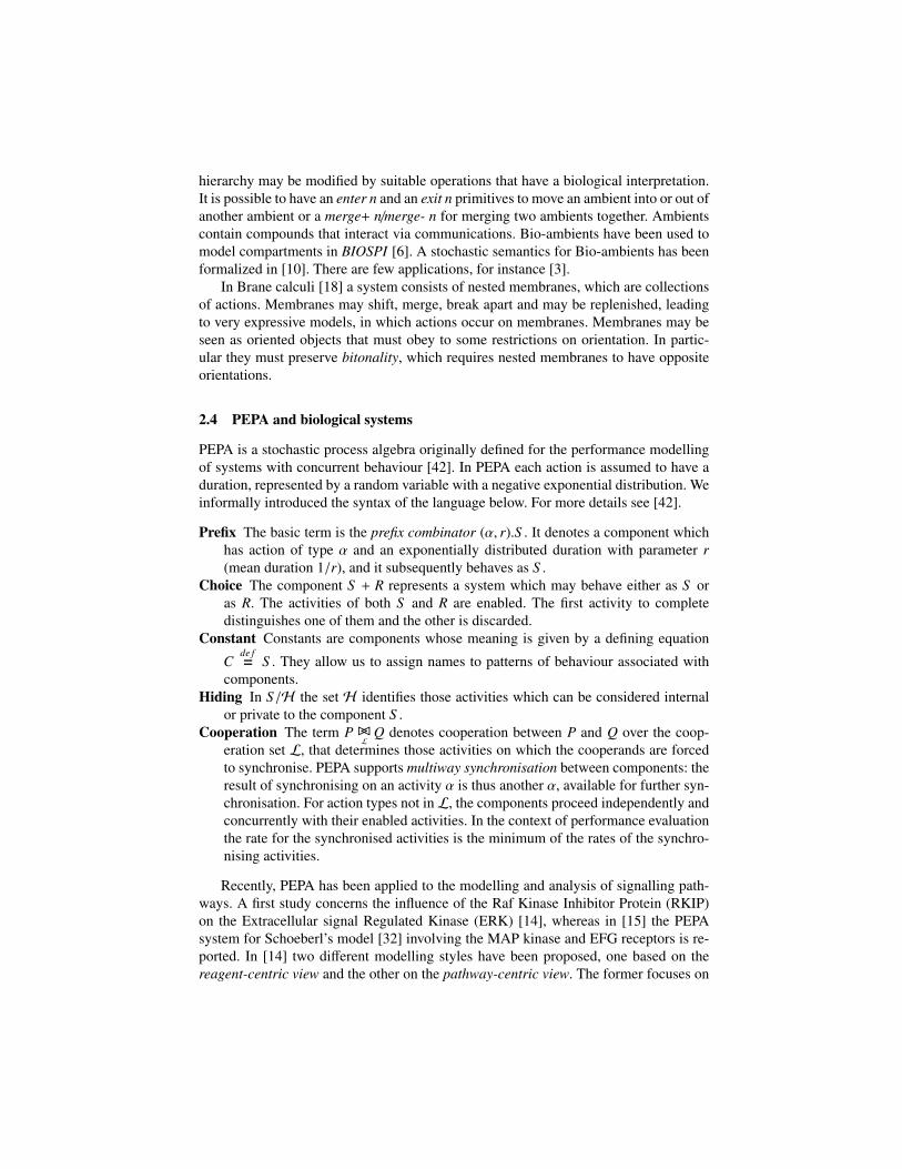
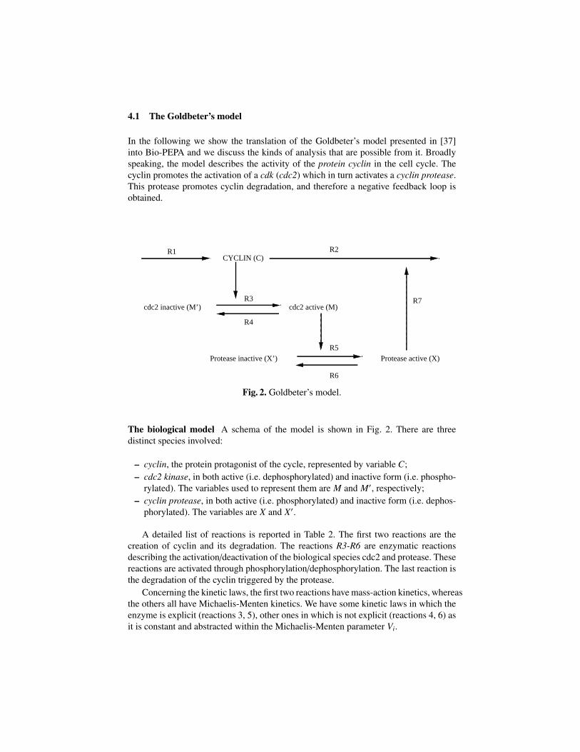
In the following we show the translation of the Goldbeter’s model presented in [37]into Bio-PEPA and we discuss the kinds of analysis that are possible from it. Broadlyspeaking, the model describes the activity of the protein cyclin in the cell cycle. Thecyclin promotes the activation of a cdk (cdc2) which in turn activates a cyclin protease.This protease promotes cyclin degradation, and therefore a negative feedback loop isobtained.

CYCLIN (C)

cdc2 inactive (M’)

Protease inactive (X’) Protease active (X)

R1

R3

R4

R7cdc2 active (M)

R2

R6

R5

Fig. 2. Goldbeter’s model.

The biological model A schema of the model is shown in Fig. 2. There are threedistinct species involved:

– cyclin, the protein protagonist of the cycle, represented by variable C;– cdc2 kinase, in both active (i.e. dephosphorylated) and inactive form (i.e. phospho-

rylated). The variables used to represent them are M and M′, respectively;– cyclin protease, in both active (i.e. phosphorylated) and inactive form (i.e. dephos-

phorylated). The variables are X and X′.

A detailed list of reactions is reported in Table 2. The first two reactions are thecreation of cyclin and its degradation. The reactions R3-R6 are enzymatic reactionsdescribing the activation/deactivation of the biological species cdc2 and protease. Thesereactions are activated through phosphorylation/dephosphorylation. The last reaction isthe degradation of the cyclin triggered by the protease.

Concerning the kinetic laws, the first two reactions have mass-action kinetics, whereasthe others all have Michaelis-Menten kinetics. We have some kinetic laws in which theenzyme is explicit (reactions 3, 5), other ones in which is not explicit (reactions 4, 6) asit is constant and abstracted within the Michaelis-Menten parameter Vi.

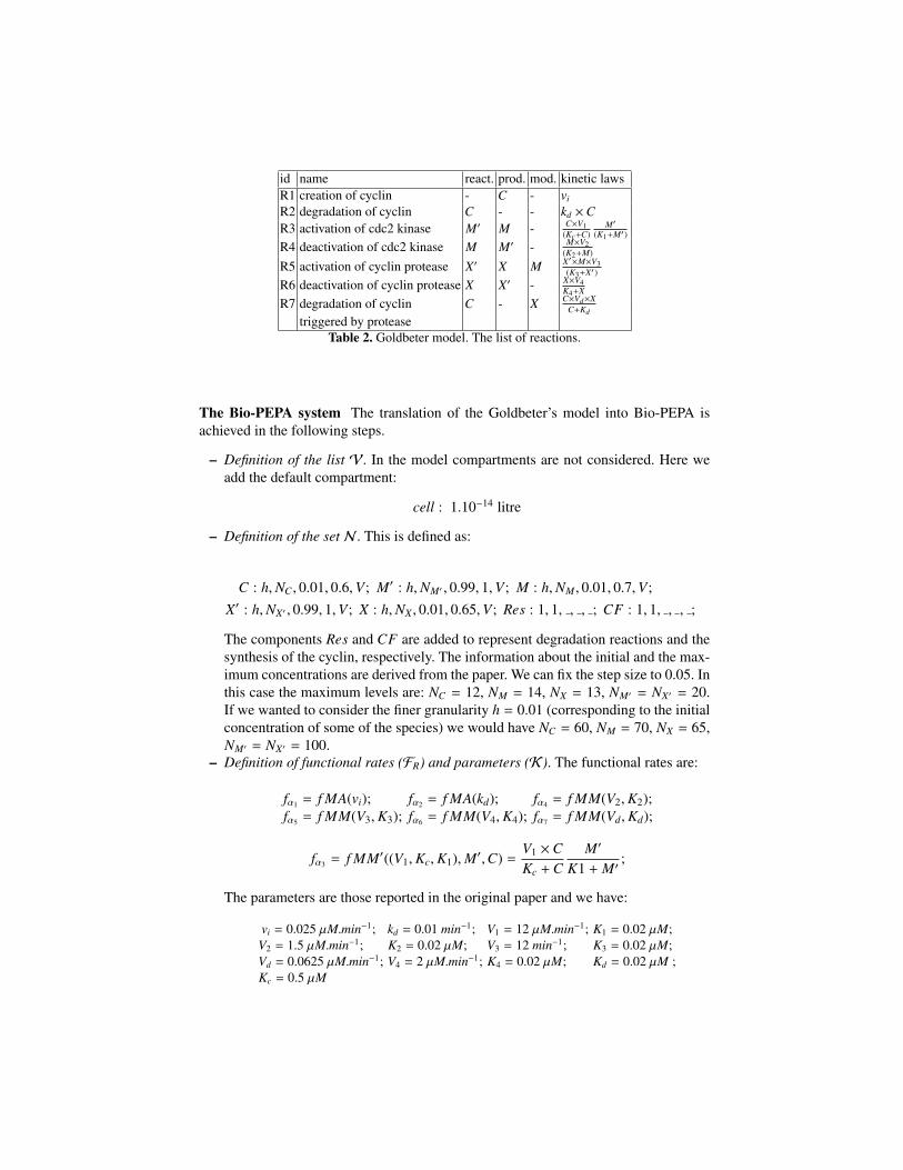
id name react. prod. mod. kinetic lawsR1 creation of cyclin - C - vi

R2 degradation of cyclin C - - kd ×CR3 activation of cdc2 kinase M′ M - C×V1

(Kc+C)M′

(K1+M′)

R4 deactivation of cdc2 kinase M M′ - M×V2(K2+M)

R5 activation of cyclin protease X′ X M X′×M×V3(K3+X′)

R6 deactivation of cyclin protease X X′ - X×V4K4+X

R7 degradation of cyclin C - X C×Vd×XC+Kd

triggered by proteaseTable 2. Goldbeter model. The list of reactions.

The Bio-PEPA system The translation of the Goldbeter’s model into Bio-PEPA isachieved in the following steps.

– Definition of the list V. In the model compartments are not considered. Here weadd the default compartment:

cell : 1.10−14 litre

– Definition of the set N . This is defined as:

C : h,NC , 0.01, 0.6,V; M′ : h,NM′ , 0.99, 1,V; M : h,NM , 0.01, 0.7,V;X′ : h,NX′ , 0.99, 1,V; X : h,NX , 0.01, 0.65,V; Res : 1, 1, , , ; CF : 1, 1, , , ;

The components Res and CF are added to represent degradation reactions and thesynthesis of the cyclin, respectively. The information about the initial and the max-imum concentrations are derived from the paper. We can fix the step size to 0.05. Inthis case the maximum levels are: NC = 12, NM = 14, NX = 13, NM′ = NX′ = 20.If we wanted to consider the finer granularity h = 0.01 (corresponding to the initialconcentration of some of the species) we would have NC = 60, NM = 70, NX = 65,NM′ = NX′ = 100.

– Definition of functional rates (FR) and parameters (K). The functional rates are:

fα1 = f MA(vi); fα2 = f MA(kd); fα4 = f MM(V2,K2);fα5 = f MM(V3,K3); fα6 = f MM(V4,K4); fα7 = f MM(Vd,Kd);

fα3 = f MM′((V1,Kc,K1),M′,C) =V1 ×CKc +C

M′

K1 + M′;

The parameters are those reported in the original paper and we have:

vi = 0.025 µM.min−1; kd = 0.01 min−1; V1 = 12 µM.min−1; K1 = 0.02 µM;V2 = 1.5 µM.min−1; K2 = 0.02 µM; V3 = 12 min−1; K3 = 0.02 µM;Vd = 0.0625 µM.min−1; V4 = 2 µM.min−1; K4 = 0.02 µM; Kd = 0.02 µM ;Kc = 0.5 µM

– Definition of species components (Comp) and of the model component (P).

Cdef= (α1, 1)↑C + (α2, 1)↓C + (α7, 1)↓C + (α3, 1) ⊕C;

M′def= (α4, 1)↑M′ + (α3, 1)↓M′;

Mdef= (α3, 1)↑M + (α4, 1)↓M + (α5, 1) ⊕ M;

X′def= (α6, 1)↑X′ + (α5, 1)↓X′;

Xdef= (α5, 1)↑X + (α6, 1)↓X + (α7, 1) ⊕ X;

Resdef= (α2, 1) � Res; CF = (α1, 1) � CF;

C(l0C) BC{α3 }

M(l0M) BC{α3 ,α4 }

M′

(l0M′ ) BC{α5 ,α7 }

X(l0X) BC{α5 ,α6 }

X′

(l0X′ ) BC{α2 }

Res(0) BC{α1 }

CF(1)

The levels represent the initial values of the system and are set to l0C = l0M = l0X =

0 and l0M′ = l0X′ = 20.

Analysis In the following we report some observations about the analysis of the Bio-PEPA system.

SLTS and CTMC By considering the step size h = 0.05 and the number of levels givenin the Bio-PEPA system we obtain a CTMC with 52 states and 185 transitions. Thestates are described by the vector:

(C(lC),M′(lM′ ),M(lM), X′(lX′ ), X(lX))

where the different components can assume different values according to the possiblenumber of levels for each species. This CTMC is not reported.

In the following we present a simpler CTMC for our model, obtained assumingh = 1 and considering only two levels for each species. The vector N is modifiedaccordingly. We show how to define the states and the transition rates of this CTMCstarting from the Bio-PEPA system and the associated transition system. The initial sit-uation is with C, M and X absent (0) and the other elements present (1). The initial stateis (C(0),M′(1),M(0), X′(1), X(0)). Figure 3 reports the stochastic transition system inthis simplified case.

The numbers indicate the different transitions. Each transition is characterized by alabel γi containing the information about the action type and the rate. We have:

γ1 = (α1, r1) γ2 = (α2, r2) γ3 = (α3, r3) γ4 = (α4, r4)γ5 = (α5, r5) γ6 = (α6, r6) γ7 = (α4, r7) γ8 = (α3, r8)γ9 = (α1, r9) γ10 = (α2, r10) γ11 = (α7, r11) γ12 = (α4, r12)γ13 = (α3, r13) γ14 = (α5, r14) γ15 = (α6, r15) γ16 = (α4, r16)γ17 = (α2, r17) γ18 = (α6, r18) γ19 = (α1, r19) γ20 = (α2, r20)γ21 = (α7, r21) γ22 = (α1, r22) γ23 = (α6, r23)

where

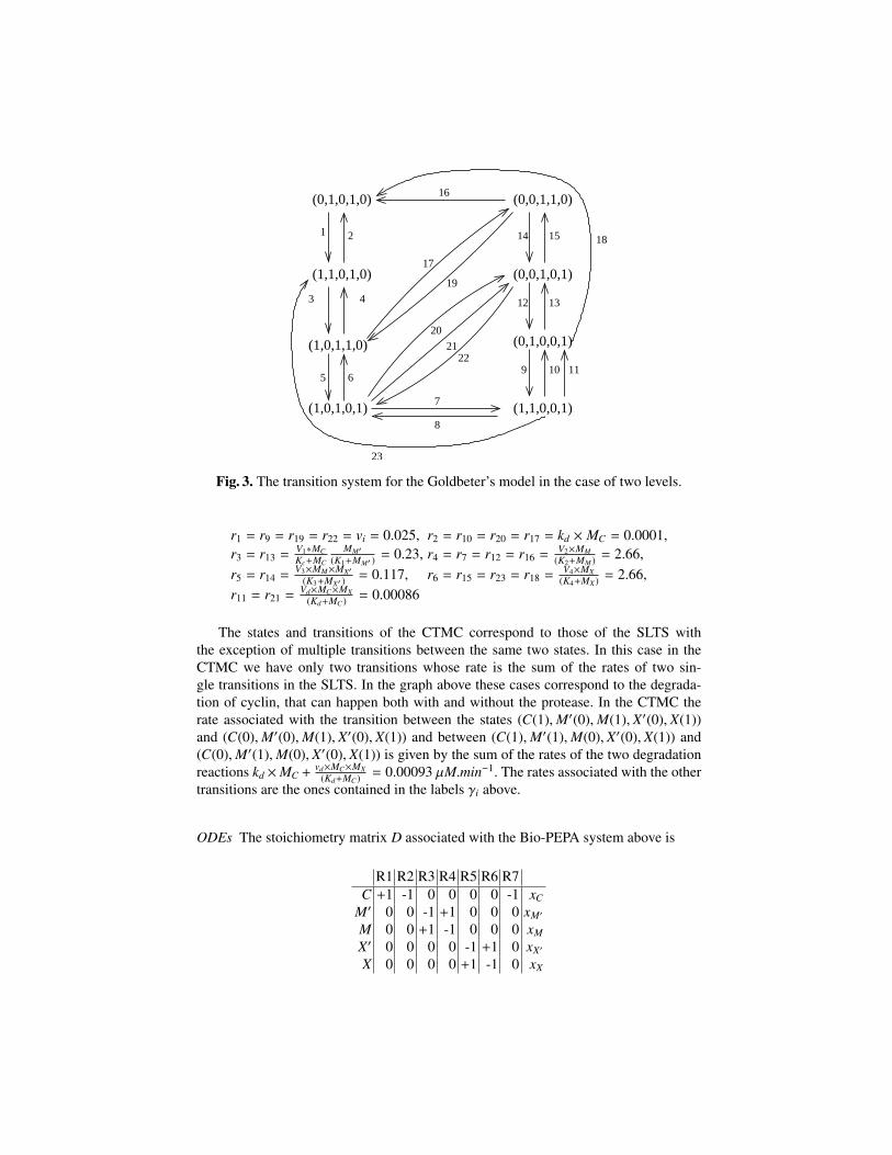
(0,0,1,1,0)(0,1,0,1,0)

(0,1,0,0,1)(1,0,1,1,0)

(1,1,0,1,0) (0,0,1,0,1)

(1,0,1,0,1) (1,1,0,0,1)

43

16

5 6

8

7

1 2 1814 15

12 13

9 10 1122

21

20

19

17

23

Fig. 3. The transition system for the Goldbeter’s model in the case of two levels.

r1 = r9 = r19 = r22 = vi = 0.025, r2 = r10 = r20 = r17 = kd × MC = 0.0001,r3 = r13 =

V1∗MCKc+MC

MM′

(K1+MM′ )= 0.23, r4 = r7 = r12 = r16 =

V2×MM(K2+MM ) = 2.66,

r5 = r14 =V3×MM×MX′

(K3+MX′ )= 0.117, r6 = r15 = r23 = r18 =

V4×MX(K4+MX ) = 2.66,

r11 = r21 =Vd×MC×MX

(Kd+MC ) = 0.00086

The states and transitions of the CTMC correspond to those of the SLTS withthe exception of multiple transitions between the same two states. In this case in theCTMC we have only two transitions whose rate is the sum of the rates of two sin-gle transitions in the SLTS. In the graph above these cases correspond to the degrada-tion of cyclin, that can happen both with and without the protease. In the CTMC therate associated with the transition between the states (C(1),M′(0),M(1), X′(0), X(1))and (C(0),M′(0),M(1), X′(0), X(1)) and between (C(1),M′(1),M(0), X′(0), X(1)) and(C(0),M′(1),M(0), X′(0), X(1)) is given by the sum of the rates of the two degradationreactions kd ×MC +

vd×MC×MX(Kd+MC ) = 0.00093 µM.min−1. The rates associated with the other

transitions are the ones contained in the labels γi above.

ODEs The stoichiometry matrix D associated with the Bio-PEPA system above is

R1 R2 R3 R4 R5 R6 R7C +1 -1 0 0 0 0 -1 xC

M′ 0 0 -1 +1 0 0 0 xM′

M 0 0 +1 -1 0 0 0 xM

X′ 0 0 0 0 -1 +1 0 xX′

X 0 0 0 0 +1 -1 0 xX

The vector that contains the kinetic laws is:

vTKL =

(vi × 1, kd × xC ,

V1 × xC

Kc + xC

xM′

(K1 + xM′ ),

V2 × xM

(K2 + xM),

V3 × xM × xX′

(K3 + xX′ ),

V4 × xX

(K4 + xX),

vd × xC × xX

(Kd + xC)

)where “T” indicates the transpose of a vector (or a matrix). The system of ODEs isobtained as dx

dt = D × vKL, with xT := (xC , xM′ , xM , xX′ , xX), the vector of the speciesvariables:

dxC

dt= vi × 1 − kd × xC −

vd × xC × xX

(Kd + xC);

dxM′

dt= −

V1 × xC

Kc + xC×

xM′

(K1 + xM′ )+

V2 × xM

(K2 + xM);

dxM

dt=

V1 × xC

Kc + xC×

xM′

(K1 + xM′ )−

V2 × xM

(K2 + xM);

dxX′

dt= −

V3 × xM × xX′

(K3 + xX′ )+

V4 × xX

(K4 + xX);

dxX

dt=

V3 × xM × xX′

(K3 + xX′ )−

V4 × xX

(K4 + xX);

The initial conditions are the ones reported in the set N . It is worth noting that thesystem is equivalent, after some arithmetic manipulations, to the ODE model presentedin [37]. The analysis of the model using ODEs is reported in Figure 11. The graphscoincide with results in the original paper.

PRISM The full translation of the model into PRISM is reported in the Appendix A. Thenumber of levels, the maximum concentrations and the parameters used in the kineticlaws are expressed using global constants. For each species a module is constructed.The module representing the cyclin is:

module cyclincyclin : [0..Nc] init 0;[creationC] cyclin < Nc→ (cyclin′ = cyclin + 1);[degradationC] cyclin > 0→ (cyclin′ = cyclin − 1);[activationM] cyclin > 0→ (cyclin′ = cyclin);[degradationCX] cyclin > 0→ (cyclin′ = cyclin − 1);endmodule

The variable cyclin is local and represents the species “cyclin”. The possible valuesare [0..Nc] (where Nc is the maximum level for cyclin) and the initial value is set to0. Cyclin is involved in four different reactions represented by four commands. Thename in the square brackets denotes the reaction. The guards are defined accordingto whether cyclin is a reactant, product or modifier of the reaction (this can be derivedfrom the Bio-PEPA specification of the model). The rate associated with each commandis “1” with the exception of the command in the module describing the functional rates.The functional rates are defined in a specific module.

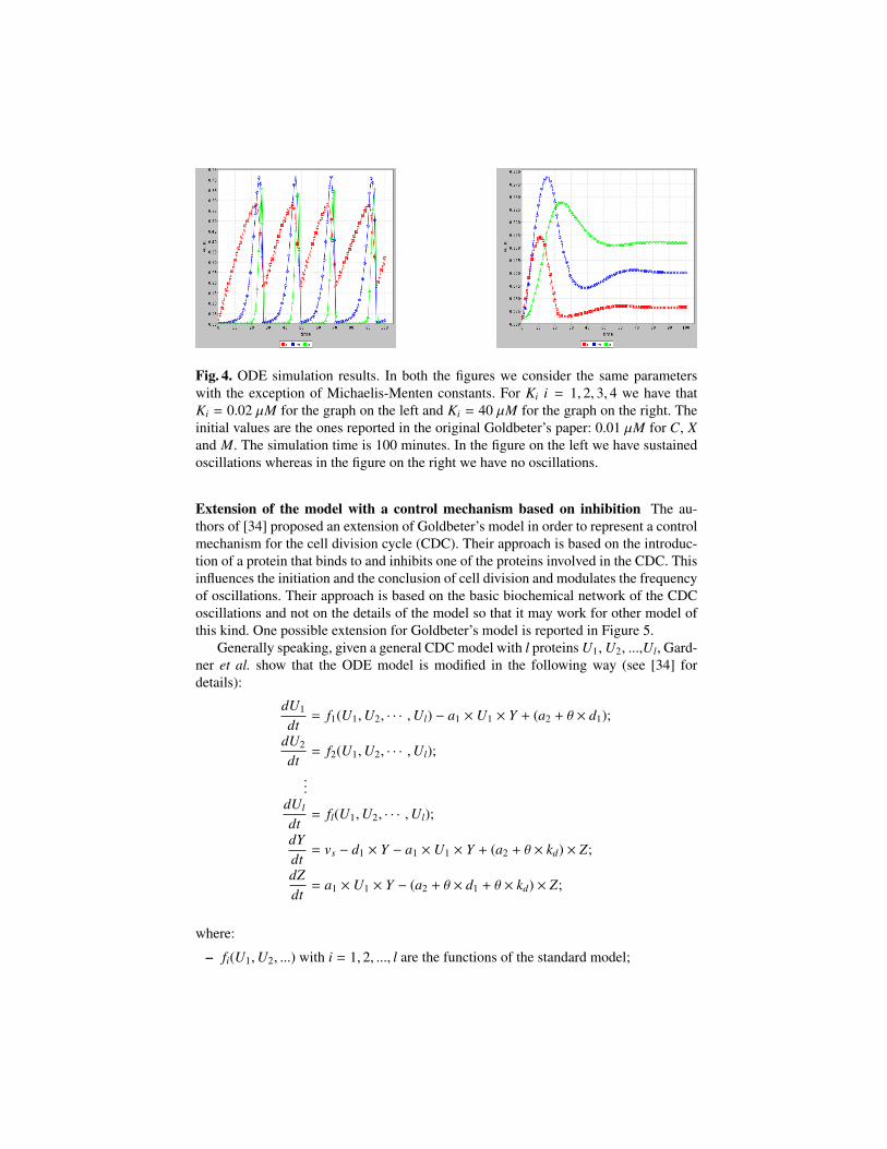
Fig. 4. ODE simulation results. In both the figures we consider the same parameterswith the exception of Michaelis-Menten constants. For Ki i = 1, 2, 3, 4 we have thatKi = 0.02 µM for the graph on the left and Ki = 40 µM for the graph on the right. Theinitial values are the ones reported in the original Goldbeter’s paper: 0.01 µM for C, Xand M. The simulation time is 100 minutes. In the figure on the left we have sustainedoscillations whereas in the figure on the right we have no oscillations.

Extension of the model with a control mechanism based on inhibition The au-thors of [34] proposed an extension of Goldbeter’s model in order to represent a controlmechanism for the cell division cycle (CDC). Their approach is based on the introduc-tion of a protein that binds to and inhibits one of the proteins involved in the CDC. Thisinfluences the initiation and the conclusion of cell division and modulates the frequencyof oscillations. Their approach is based on the basic biochemical network of the CDCoscillations and not on the details of the model so that it may work for other model ofthis kind. One possible extension for Goldbeter’s model is reported in Figure 5.

Generally speaking, given a general CDC model with l proteins U1, U2, ...,Ul, Gard-ner et al. show that the ODE model is modified in the following way (see [34] fordetails):

dU1

dt= f1(U1,U2, · · · ,Ul) − a1 × U1 × Y + (a2 + θ × d1);

dU2

dt= f2(U1,U2, · · · ,Ul);

...dUl

dt= fl(U1,U2, · · · ,Ul);

dYdt= vs − d1 × Y − a1 × U1 × Y + (a2 + θ × kd) × Z;

dZdt= a1 × U1 × Y − (a2 + θ × d1 + θ × kd) × Z;

where:

– fi(U1,U2, ...) with i = 1, 2, ..., l are the functions of the standard model;

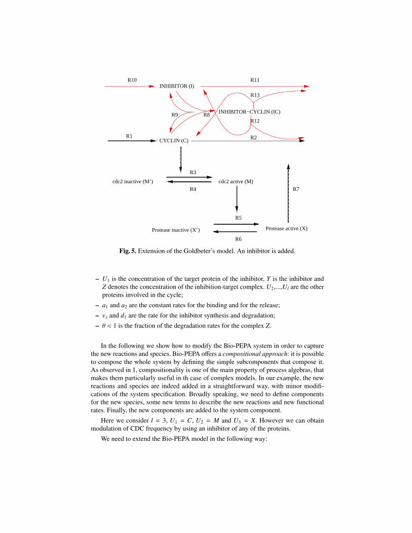
Protease inactive (X’) Protease active (X)

R7

R6

cdc2 active (M)R4

cdc2 inactive (M’)

CYCLIN (C)R1

INHIBITOR−CYCLIN (IC)

INHIBITOR (I)R10

R3

R5

R8R9

R11

R13

R12

R2

Fig. 5. Extension of the Goldbeter’s model. An inhibitor is added.

– U1 is the concentration of the target protein of the inhibitor, Y is the inhibitor andZ denotes the concentration of the inhibition-target complex. U2,...,Ul are the otherproteins involved in the cycle;

– a1 and a2 are the constant rates for the binding and for the release;

– vs and d1 are the rate for the inhibitor synthesis and degradation;

– θ < 1 is the fraction of the degradation rates for the complex Z.

In the following we show how to modify the Bio-PEPA system in order to capturethe new reactions and species. Bio-PEPA offers a compositional approach: it is possibleto compose the whole system by defining the simple subcomponents that compose it.As observed in 1, compositionality is one of the main property of process algebras, thatmakes them particularly useful in th case of complex models. In our example, the newreactions and species are indeed added in a straightforward way, with minor modifi-cations of the system specification. Broadly speaking, we need to define componentsfor the new species, some new terms to describe the new reactions and new functionalrates. Finally, the new components are added to the system component.

Here we consider l = 3, U1 = C, U2 = M and U3 = X. However we can obtainmodulation of CDC frequency by using an inhibitor of any of the proteins.

We need to extend the Bio-PEPA model in the following way:

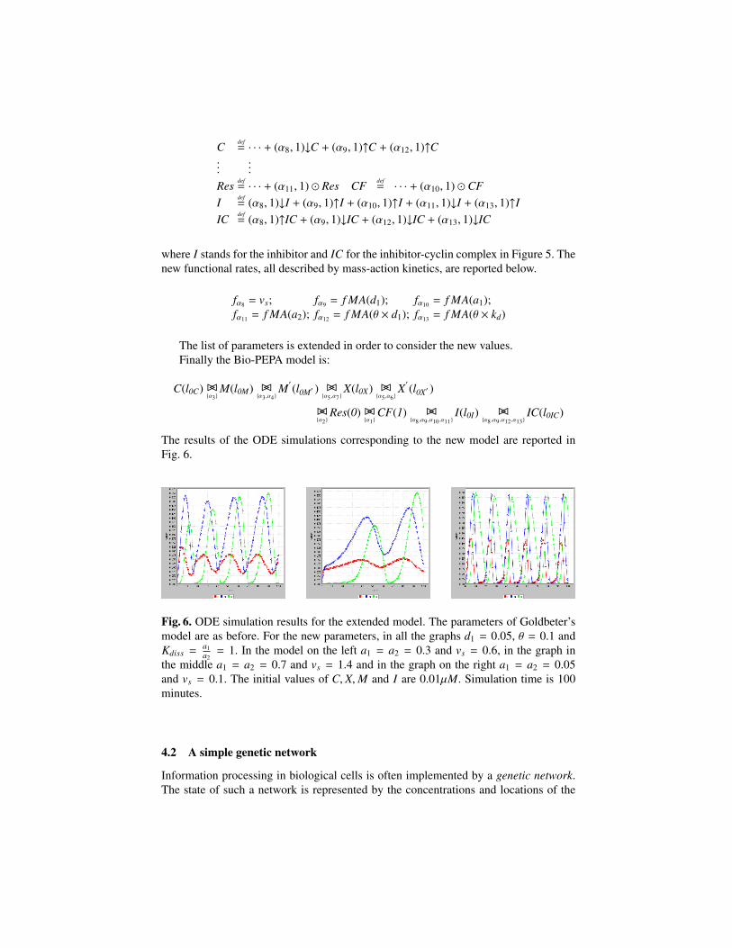
Cdef= · · · + (α8, 1)↓C + (α9, 1)↑C + (α12, 1)↑C

......

Resdef= · · · + (α11, 1) � Res CF

def= · · · + (α10, 1) � CF

Idef= (α8, 1)↓I + (α9, 1)↑I + (α10, 1)↑I + (α11, 1)↓I + (α13, 1)↑I

ICdef= (α8, 1)↑IC + (α9, 1)↓IC + (α12, 1)↓IC + (α13, 1)↓IC

where I stands for the inhibitor and IC for the inhibitor-cyclin complex in Figure 5. Thenew functional rates, all described by mass-action kinetics, are reported below.

fα8 = vs; fα9 = f MA(d1); fα10 = f MA(a1);fα11 = f MA(a2); fα12 = f MA(θ × d1); fα13 = f MA(θ × kd)

The list of parameters is extended in order to consider the new values.Finally the Bio-PEPA model is:

C(l0C) BC{α3 }

M(l0M) BC{α3 ,α4 }

M′

(l0M′ ) BC{α5 ,α7 }

X(l0X) BC{α5 ,α6 }

X′

(l0X′ )

BC{α2 }

Res(0) BC{α1 }

CF(1) BC{α8 ,α9 ,α10 ,α11 }

I(l0I) BC{α8 ,α9 ,α12 ,α13 }

IC(l0IC)

The results of the ODE simulations corresponding to the new model are reported inFig. 6.

Fig. 6. ODE simulation results for the extended model. The parameters of Goldbeter’smodel are as before. For the new parameters, in all the graphs d1 = 0.05, θ = 0.1 andKdiss =

a1a2= 1. In the model on the left a1 = a2 = 0.3 and vs = 0.6, in the graph in

the middle a1 = a2 = 0.7 and vs = 1.4 and in the graph on the right a1 = a2 = 0.05and vs = 0.1. The initial values of C, X,M and I are 0.01µM. Simulation time is 100minutes.

4.2 A simple genetic network

Information processing in biological cells is often implemented by a genetic network.The state of such a network is represented by the concentrations and locations of the

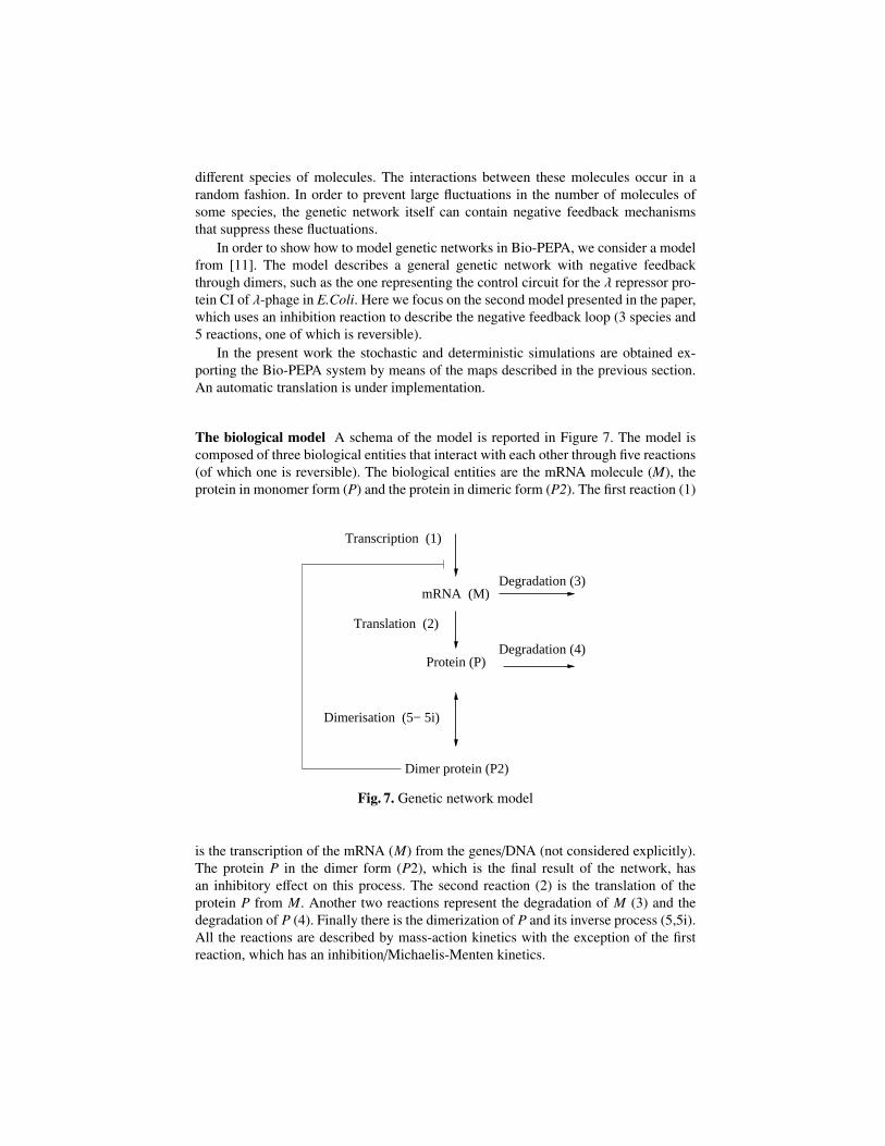
different species of molecules. The interactions between these molecules occur in arandom fashion. In order to prevent large fluctuations in the number of molecules ofsome species, the genetic network itself can contain negative feedback mechanismsthat suppress these fluctuations.

In order to show how to model genetic networks in Bio-PEPA, we consider a modelfrom [11]. The model describes a general genetic network with negative feedbackthrough dimers, such as the one representing the control circuit for the λ repressor pro-tein CI of λ-phage in E.Coli. Here we focus on the second model presented in the paper,which uses an inhibition reaction to describe the negative feedback loop (3 species and5 reactions, one of which is reversible).

In the present work the stochastic and deterministic simulations are obtained ex-porting the Bio-PEPA system by means of the maps described in the previous section.An automatic translation is under implementation.

The biological model A schema of the model is reported in Figure 7. The model iscomposed of three biological entities that interact with each other through five reactions(of which one is reversible). The biological entities are the mRNA molecule (M), theprotein in monomer form (P) and the protein in dimeric form (P2). The first reaction (1)

mRNA (M)Degradation (3)

Protein (P)Degradation (4)

Dimer protein (P2)

Dimerisation (5− 5i)

Transcription (1)

Translation (2)

Fig. 7. Genetic network model

is the transcription of the mRNA (M) from the genes/DNA (not considered explicitly).The protein P in the dimer form (P2), which is the final result of the network, hasan inhibitory effect on this process. The second reaction (2) is the translation of theprotein P from M. Another two reactions represent the degradation of M (3) and thedegradation of P (4). Finally there is the dimerization of P and its inverse process (5,5i).All the reactions are described by mass-action kinetics with the exception of the firstreaction, which has an inhibition/Michaelis-Menten kinetics.

The Bio-PEPA system The translation of the model in Bio-PEPA is based on thefollowing steps:

– Definition of compartments. The only compartment is defined as vcell : 1 (nM)−1.– Definition of the setN . We need to define the step size and the number of levels for

each species:

M : hM ,NM; P : hP,NP; P2 : hP2,NP2; Res : 1, 1; CF : 1, 1

We omit the information concerning the initial and maximum concentrations. Fur-thermore the compartments are not considered as all the species are in the samecompartment. From the original paper the maximum concentrations are MN =

1 nM, MP = 60 nM and MP2 = 180 nM. We can consider hM = 1 nM andhP = hP2 = 30 nM. Indeed the stoichiometry of P in the dimerization reactionis 2 and we need to consider at least two levels for P. The maximum levels for thethree species are: NM = 1, NP = 2 and NP2 = 6.

– Definition of the set of functional rates FR.

fα1 = f I((v,KM), [P2,CF]) = v×CFKM+P2 ;

fα2 = f MA(k2); fα3 = f MA(k3); fα4 = f MA(k4);fα5 = f MA(k5); fα5i = f MA(k5i)

where the suffix of the action type α refers to the number of the reaction as reportedin Fig. 7.

– Definition of the set of parameters. The parameter values are

KM = 356 nM; v = 2.19 s−1; k2 = 0.043 s−1; k3 = 0.0039 s−1;k4 = 0.0007 s−1; k5 = 0.025 s−1nM−1; k5i = 0.5 s−1

– Definition of the set of species components and of the model component.

Mdef= (α2, 1) ⊕ M + (α3, 1)↓M + (α1, 1)↑M;

Pdef= (α4, 1)↓P + (α5, 2)↓P + (α5i, 2)↑P) + (α2, 0)↑P;

P2 def= (α1, 1) P2 + (α5i, 1)↓P2 + (α5, 1)↑P2;

Resdef= (α3, 1) � Res + (α4, 1) � Res;

CFdef= (α1, 1) � CF;

(((CF(1) BC{α1 }

M(0)) BC{α2 }

P(0)) BC{α5 ,α5i }

P2(0)) BC{α3 ,α4 }

Res(0)

Analysis The model is amenable to a number of different analyses as we report in thefollowing paragraphs.

SLTS and CTMC From the Bio-PEPA model we can derive the SLTS and the CTMC.The transition system consists of 42 states and 108 transitions, in the case we considerthe information about species listed above.

The states are described by the levels of the single components. Specifically, we candefine a state using a vector (CF(l1),M(l2), P(l3), P2(l4),Res(l5)),where li i = 1, ..., 5represents the level of each component. The parameter li can assume the values 0 and 1in the case of M, the values 0, 1, 2 for P and values between 0 and 6 for P2. Res andCF can assume only one value (0 and 1, respectively). The labels γt of the stochastictransition system contain the action type α j and the rate rα j , calculated by applyingthe associated function fα j to the quantitative information collected in the labels of thecapability relation and dividing this by the step size of the reactants/products involvedin the reaction. These rates are the ones associated with the CTMC transitions.

ODEs and Gillespie A second kind of analysis concerns differential equations. Thestoichiometry matrix D associated with the system is

R1 R2 R3 R4 R5 R5iCF 0 0 0 0 0 0 xCF

M +1 0 -1 0 0 0 x1

P 0 +1 0 -1 -2 +2 x2

P2 0 0 0 0 +1 -1 x3

Res 0 0 0 0 0 0 xRes

The kinetic-law vector is vTKL = ( v×xCF

K+x3; k2 × x1; k3 × x1; k4 × x2; k5 × x2

2; k5i × x3). Thesystem of ODEs is obtained as dx

dt = D × vKL:

dx1

dt=

v × 1K + x3

− k3 × x1

dx2

dt= k2 × x1 − k4 × x2 − 2 × k5 × x2

2 + 2 × k5i × x3

dx2

dt= k5 × x2

2 − k5i × x3

The derivation of the Gillespie’s simulation model is straightforward and not re-ported here.

The simulation results are depicted in Figure 12. We consider both deterministicand stochastic simulation. The two simulation graphs show the same behaviour (withthe exception of some noise in the Gillespie’s simulation), as expected.

PRISM The full translation of the model into PRISM is reported in [?]. Each species isrepresented by a PRISM module and the reactions in which it is involved are capturedby commands. In the following we report the definition of the modules representing theprotein in the monomer and dimer form respectively.

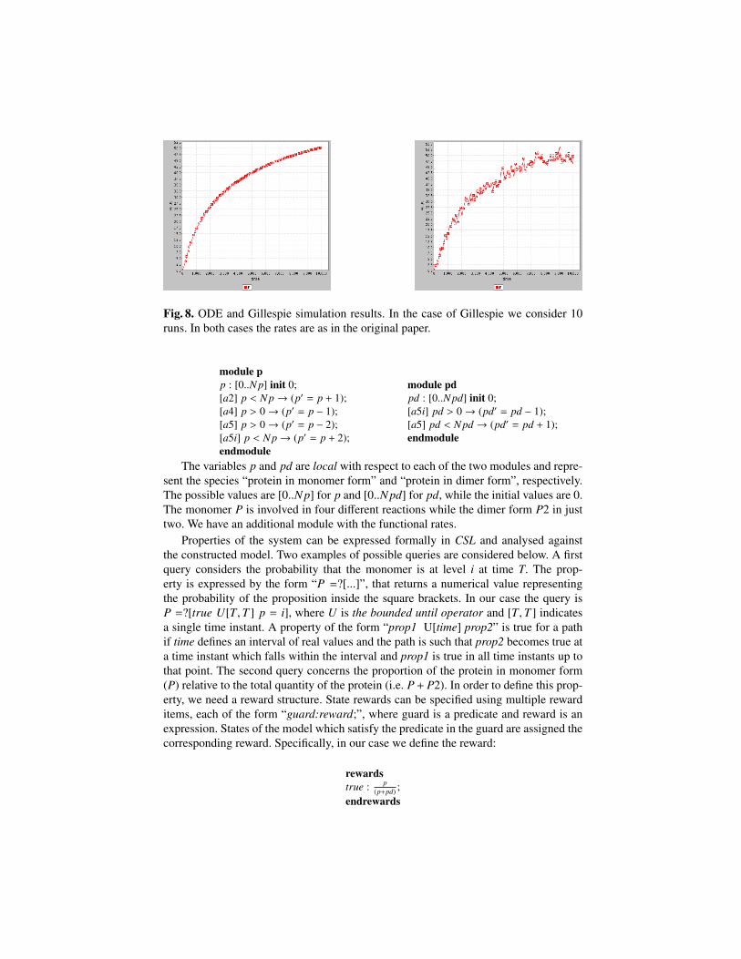
Fig. 8. ODE and Gillespie simulation results. In the case of Gillespie we consider 10runs. In both cases the rates are as in the original paper.

module pp : [0..N p] init 0;[a2] p < N p→ (p′ = p + 1);[a4] p > 0→ (p′ = p − 1);[a5] p > 0→ (p′ = p − 2);[a5i] p < N p→ (p′ = p + 2);endmodule

module pdpd : [0..N pd] init 0;[a5i] pd > 0→ (pd′ = pd − 1);[a5] pd < N pd → (pd′ = pd + 1);endmodule

The variables p and pd are local with respect to each of the two modules and repre-sent the species “protein in monomer form” and “protein in dimer form”, respectively.The possible values are [0..N p] for p and [0..N pd] for pd, while the initial values are 0.The monomer P is involved in four different reactions while the dimer form P2 in justtwo. We have an additional module with the functional rates.

Properties of the system can be expressed formally in CSL and analysed againstthe constructed model. Two examples of possible queries are considered below. A firstquery considers the probability that the monomer is at level i at time T. The prop-erty is expressed by the form “P =?[...]”, that returns a numerical value representingthe probability of the proposition inside the square brackets. In our case the query isP =?[true U[T,T ] p = i], where U is the bounded until operator and [T,T ] indicatesa single time instant. A property of the form “prop1 U[time] prop2” is true for a pathif time defines an interval of real values and the path is such that prop2 becomes true ata time instant which falls within the interval and prop1 is true in all time instants up tothat point. The second query concerns the proportion of the protein in monomer form(P) relative to the total quantity of the protein (i.e. P+ P2). In order to define this prop-erty, we need a reward structure. State rewards can be specified using multiple rewarditems, each of the form “guard:reward;”, where guard is a predicate and reward is anexpression. States of the model which satisfy the predicate in the guard are assigned thecorresponding reward. Specifically, in our case we define the reward:

rewardstrue : p

(p+pd) ;endrewards

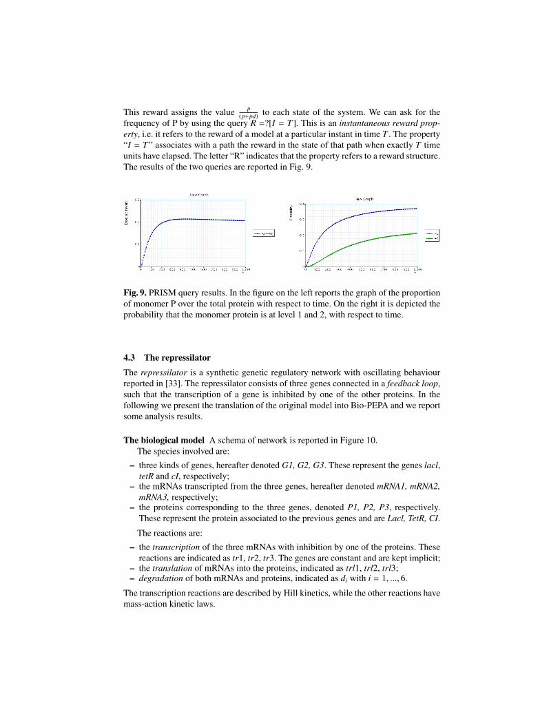
This reward assigns the value p(p+pd) to each state of the system. We can ask for the

frequency of P by using the query R =?[I = T ]. This is an instantaneous reward prop-erty, i.e. it refers to the reward of a model at a particular instant in time T . The property“I = T” associates with a path the reward in the state of that path when exactly T timeunits have elapsed. The letter “R” indicates that the property refers to a reward structure.The results of the two queries are reported in Fig. 9.

Fig. 9. PRISM query results. In the figure on the left reports the graph of the proportionof monomer P over the total protein with respect to time. On the right it is depicted theprobability that the monomer protein is at level 1 and 2, with respect to time.

4.3 The repressilator

The repressilator is a synthetic genetic regulatory network with oscillating behaviourreported in [33]. The repressilator consists of three genes connected in a feedback loop,such that the transcription of a gene is inhibited by one of the other proteins. In thefollowing we present the translation of the original model into Bio-PEPA and we reportsome analysis results.

The biological model A schema of network is reported in Figure 10.The species involved are:

– three kinds of genes, hereafter denoted G1, G2, G3. These represent the genes lacl,tetR and cI, respectively;

– the mRNAs transcripted from the three genes, hereafter denoted mRNA1, mRNA2,mRNA3, respectively;

– the proteins corresponding to the three genes, denoted P1, P2, P3, respectively.These represent the protein associated to the previous genes and are Lacl, TetR, CI.

The reactions are:

– the transcription of the three mRNAs with inhibition by one of the proteins. Thesereactions are indicated as tr1, tr2, tr3. The genes are constant and are kept implicit;

– the translation of mRNAs into the proteins, indicated as trl1, trl2, trl3;– degradation of both mRNAs and proteins, indicated as di with i = 1, ..., 6.

The transcription reactions are described by Hill kinetics, while the other reactions havemass-action kinetic laws.

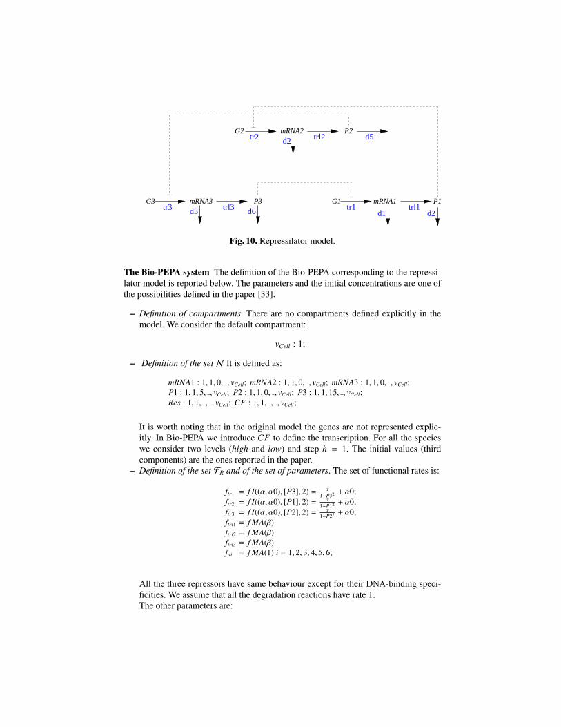
P2 mRNA2 G2

G3 mRNA3 P3 G1 mRNA1 P1

trl2tr2 d2 d5

tr1 trl1d2d1d6trl3tr3 d3

Fig. 10. Repressilator model.

The Bio-PEPA system The definition of the Bio-PEPA corresponding to the repressi-lator model is reported below. The parameters and the initial concentrations are one ofthe possibilities defined in the paper [33].

– Definition of compartments. There are no compartments defined explicitly in themodel. We consider the default compartment:

vCell : 1;

– Definition of the set N It is defined as:

mRNA1 : 1, 1, 0, , vCell; mRNA2 : 1, 1, 0, , vCell; mRNA3 : 1, 1, 0, , vCell;P1 : 1, 1, 5, , vCell; P2 : 1, 1, 0, , vCell; P3 : 1, 1, 15, , vCell;Res : 1, 1, , , vCell; CF : 1, 1, , , vCell;

It is worth noting that in the original model the genes are not represented explic-itly. In Bio-PEPA we introduce CF to define the transcription. For all the specieswe consider two levels (high and low) and step h = 1. The initial values (thirdcomponents) are the ones reported in the paper.

– Definition of the set FR and of the set of parameters. The set of functional rates is:

ftr1 = f I((α, α0), [P3], 2) = α1+P32 + α0;

ftr2 = f I((α, α0), [P1], 2) = α1+P12 + α0;

ftr3 = f I((α, α0), [P2], 2) = α1+P22 + α0;

ftrl1 = f MA(β)ftrl2 = f MA(β)ftrl3 = f MA(β)fdi = f MA(1) i = 1, 2, 3, 4, 5, 6;

All the three repressors have same behaviour except for their DNA-binding speci-ficities. We assume that all the degradation reactions have rate 1.The other parameters are:

α = 250; α0 = 0; β = 5

These parameters have the following meaning:• α0 is the number of protein copies per cell produced from a given promoter

type during growth in the presence of saturing amounts of the repressor. In thecase of the absence of the repressor this number is α0 + α;

• β is the ratio of the protein decay rate to the mRNA decay rate.– Definition of the species components. The species components are:

mRNA1def= (d1, 1)↓mRNA1 + (tr1, 1)↑mRNA1 + (trl1, 1) ⊕ mRNA1;

mRNA2def= (d2, 1)↓mRNA2 + (tr2, 1)↑mRNA2 + (trl2, 1) ⊕ mRNA2;

mRNA3def= (d3, 1)↓mRNA3 + (tr3, 1)↑mRNA3 + (trl3, 1) ⊕ mRNA3;

P1def= (d4, 1)↓P1 + (trl1, 1)↑P1 + (tr3, 1) P1;

P2def= (d5, 1)↓P2 + (trl2, 1)↑P2 + (tr1, 1) P2;

P3def= (d6, 1)↓P3 + (trl3, 1)↑P3 + (tr2, 1) P3;

CFdef= (tr1, 1) �CF + (tr1, 1) �CF + (tr1, 1) �CF;

Resdef= (d1, 1) � Res + (d2, 1) � Res + (d3, 1) � Res+

(d4, 1) � Res + (d5, 1) � Res + (d6, 1) � Res;

– Definition of the model component. The model is defined as:

((((((M1(lM10) <> M2(lM20)) BCM3(lM30)) BC{trl1,tr3}

P1(lP10)) BC{trl2,tr1}

P2(lP20)) BC{trl3,tr2}

P3(lP30)) BC{tr1,tr2,tr3}

BC{tr1,tr2,tr3}

CF(1)) BC{d1,d2,d3,d4,d5,d6}

Res(0)

The initial levels are defined according to the initial values of the model.

Analysis We consider both ODEs and stochastic simulation by Gillespie. The analysisresults are reported in Figures 11 and 12. In Figure 11 we have used the parameters re-ported in the paper. On the left, the ODE simulation results are reported. An oscillatingbehaviour is shown by all the three proteins. On the right stochastic simulation, aver-aged over 100 runs, is reported. In this case the average oscillating behaviour becomesweaker after some time. The difference between determistic and stochastic simulationsis probably due to the use of Hill kinetics with Gillespie. Indeed, as discussed in Section[?] the use of this kinetic law with Gillespie can lead to some wrong results. Nothe thatvarying the values of α and β for the different elements we obtain different amplitudesfor the oscillations. In the case of Figure 12, the three proteins reach a steady state, bothwith ODE and stochastic simulation.

5 Conclusions and future perspectives

In this paper we have presented Bio-PEPA, a modification of the process algebra PEPAfor the modelling and the analysis of biochemical networks. Bio-PEPA allows us to

Fig. 11. Analysis of the model: ODE (on the left) and Gillespie (on the right). Theparameters are the ones reported in the text. In the case of Gillespie’s simulation 100runs are considered.

Fig. 12. Analysis of the model: ODE (on the left) and Gillespie (on the right). Theparameters are different from the ones reported in the text. The parameter α0 is 25and the initial values are P1 = 5, P2 = 10 and P3 = 15. In Gillespie, 100 runs areconsidered.

represent explicitly some features of biochemical networks, such as stoichiometry andgeneral kinetic laws. Thus not only elementary reactions with constant rates, but alsocomplex reactions described by general kinetic laws can be considered. Indeed eachreaction in the model is associated with an action type and with a functional rate. Thepotential to consider various kinds of kinetic laws permits us to model a vast numberof biochemical networks. Indeed complex reactions are frequently found in models asabstractions of sequences of elementary steps and reducing to elementary reactions isoften impossible and undesirable.

Bio-PEPA in enriched with some notions of equivalence. We have presented defini-tions of isomorphism and strong bisimulation which are similar to the relations definedfor PEPA in [42]. These equivalence are quite strict. A further investigation concernsthe definition of other forms of equivalence, more appropriate for studying biologicalsystems.

A principal feature of Bio-PEPA is the possibility of mapping the system to dif-ferent kinds of analysis. In this work we have shown how to derive a CTMC from aBio-PEPA model and we have discussed the derivation of ODEs, stochastic simulationand PRISM models. Indeed Bio-PEPA has been defined as an intermediate languagefor the formal representation of the model. We have extended the definition of CTMCwith levels, defined in [16], to the case of general kinetic laws and to different levels forthe species. The main benifit of this approach is a reduction in the state space. Someassumptions are made. First of all all the species must have a finite maximum con-centration. This is to ensure a finite state space in the corresponding CTMC, makingnumerical solution feasible. However, we can have a species without a limiting value.In these cases we can consider a maximum level for the values greater than a certain(high) value. A second point concerns the assumption that all the species have the samestep size. This may be a problem when the species can have maximum concentrationsbelonging to different concentration scales. In this case some species can have only fewlevels whereas other can have many. Furthermore, some species (for instance genes)are present in the system only in few copies and in this case the representation in termsof continuous concentration is wrong. In order to handle this situation, Bio-PEPA canbe enriched with discrete variables. The possibility to consider different step sizes anddiscrete variables is a topic for future work.

The different kinds of analysis proposed for Bio-PEPA are strongly related. An areaforfurther work will concern a deeper study of these relationships, in particular for theCTMC with levels and Gillespie models. An outstanding problem is the application ofGillespie’s stochastic simulation with general kinetic laws. The approach proposed inthis work is to use Gillespie simulation also in this context, but to be careful about theinterpretation of the results. An important topic for the future will be deeper investi-gation of the relation between Gillespie simulation and general kinetic laws. Anotheraspect that needs further study is the determination of the number of concentration lev-els for each species. The definition of these numbers is critical for the definition ofthe CTMC and must be done carefully. Indeed for some analyses (ODEs and Gillespiesimulation) two levels are enough to capture the behaviour of some systems, but fornumerical analysis of the CTMC and PRISM model checking a finer granularity forlevels is necessary to capture the full behaviour of the system.

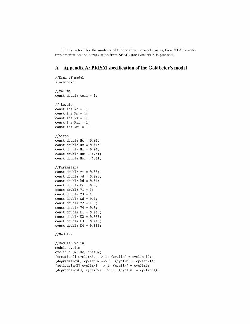
Finally, a tool for the analysis of biochemical networks using Bio-PEPA is underimplementation and a translation from SBML into Bio-PEPA is planned.

A Appendix A: PRISM specification of the Goldbeter’s model

//Kind of model

stochastic

//Volume

const double cell = 1;

// Levels

const int Nc = 1;

const int Nm = 1;

const int Nx = 1;

const int Nxi = 1;

const int Nmi = 1;

//Steps

const double Hc = 0.01;

const double Hm = 0.01;

const double Hx = 0.01;

const double Hxi = 0.01;

const double Hmi = 0.01;

//Parameters

const double vi = 0.05;

const double vd = 0.025;

const double kd = 0.01;

const double Kc = 0.5;

const double V1 = 3;

const double V3 = 1;

const double Kd = 0.2;

const double V2 = 1.5;

const double V4 = 0.5;

const double K1 = 0.005;

const double K2 = 0.005;

const double K3 = 0.005;

const double K4 = 0.005;

//Modules

//module Cyclin

module cyclin

cyclin : [0..Nc] init 0;

[creationC] cyclin<Nc --> 1: (cyclin’ = cyclin+1);

[degradationC] cyclin>0 --> 1: (cyclin’ = cyclin-1);

[activationM] cyclin>0 --> 1: (cyclin’ = cyclin);

[degradationCX] cyclin>0 --> 1: (cyclin’ = cyclin-1);

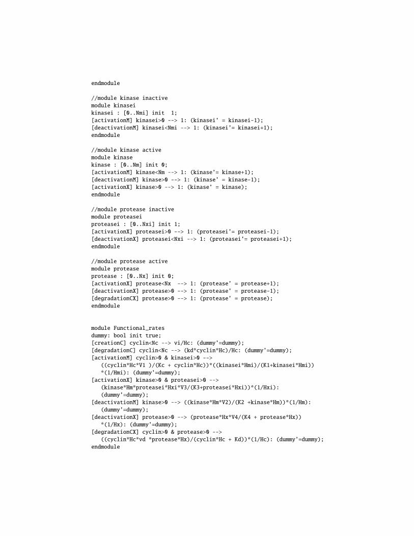
endmodule

//module kinase inactive

module kinasei

kinasei : [0..Nmi] init 1;

[activationM] kinasei>0 --> 1: (kinasei’ = kinasei-1);

[deactivationM] kinasei<Nmi --> 1: (kinasei’= kinasei+1);

endmodule

//module kinase active

module kinase

kinase : [0..Nm] init 0;

[activationM] kinase<Nm --> 1: (kinase’= kinase+1);

[deactivationM] kinase>0 --> 1: (kinase’ = kinase-1);

[activationX] kinase>0 --> 1: (kinase’ = kinase);

endmodule

//module protease inactive

module proteasei

proteasei : [0..Nxi] init 1;

[activationX] proteasei>0 --> 1: (proteasei’= proteasei-1);

[deactivationX] proteasei<Nxi --> 1: (proteasei’= proteasei+1);

endmodule

//module protease active

module protease

protease : [0..Nx] init 0;

[activationX] protease<Nx --> 1: (protease’ = protease+1);

[deactivationX] protease>0 --> 1: (protease’ = protease-1);

[degradationCX] protease>0 --> 1: (protease’ = protease);

endmodule

module Functional_rates

dummy: bool init true;

[creationC] cyclin<Nc --> vi/Hc: (dummy’=dummy);

[degradationC] cyclin<Nc --> (kd*cyclin*Hc)/Hc: (dummy’=dummy);

[activationM] cyclin>0 & kinasei>0 -->

((cyclin*Hc*V1 )/(Kc + cyclin*Hc))*((kinasei*Hmi)/(K1+kinasei*Hmi))

*(1/Hmi): (dummy’=dummy);

[activationX] kinase>0 & proteasei>0 -->

(kinase*Hm*proteasei*Hxi*V3/(K3+proteasei*Hxi))*(1/Hxi):

(dummy’=dummy);

[deactivationM] kinase>0 --> ((kinase*Hm*V2)/(K2 +kinase*Hm))*(1/Hm):

(dummy’=dummy);

[deactivationX] protease>0 --> (protease*Hx*V4/(K4 + protease*Hx))

*(1/Hx): (dummy’=dummy);

[degradationCX] cyclin>0 & protease>0 -->

((cyclin*Hc*vd *protease*Hx)/(cyclin*Hc + Kd))*(1/Hc): (dummy’=dummy);

endmodule

B AppendixB: PRISM specification of the genetic network model

//Kind of model

stochastic

//Volume

const double cell = 1*10ˆ{-6};

//Levels

const int NCF = 1;

const int Nm = 1;

const int Np = 2;

const int Npd = 6;

//Steps

const double HCF = 1;

const double Hm = 1.0;

const double Hp = 30.0;

const double Hpd = 30.0;

//Parameters

const double v = 2.19;

const double KM = 356;

const double k3 = 0.0039;

const double k2 = 0.043;

const double k4 = 0.0007;

const double k5 = 0.025;

const double k5i = 0.5;

//Modules

module CF

CF: [0..NCF] init NCF;

[a1] CF>0 --> 1: (CF’=CF);

endmodule

module p

p: [0..Np] init 0;

[a2] p<Np --> 1: (p’=p+1);

[a4] p>0 --> 1: (p’=p-1);

[a5] p>0 --> 1: (p’=p-2);

[a5i] p<Np --> 1: (p’=p+2);

endmodule

module pd

pd: [0..Npd] init 0;

[a5i] pd>0 --> 1: (pd’=pd-1);

[a5] pd<Npd --> 1: (pd’=pd+1);

endmodule

module m

m: [0..Nm] init 0;

[a1] m<Nm --> 1: (m’=m+1);

[a2] m>0 --> 1: (m’=m);

[a3] m>0 --> 1: (m’=m-1);

endmodule

module Functional_rates

dummy: bool init true;

[a1] dummy = true --> (v/(KM + pd*Hpd))*(1/Hm): (dummy’ = dummy);

[a2] dummy = true --> (k2*m*Hm)/Hm: (dummy’ = dummy);

[a3] dummy = true --> (k3*m*Hm)/Hm: (dummy’ = dummy);

[a4] dummy = true --> (k4*p*Hp)/Hp: (dummy’ = dummy);

[a5] dummy = true --> (k5*(p*Hp)ˆ2)/Hp: (dummy’ = dummy);

[a5i] dummy = true --> (k5i*pd*Hpd)/Hpd: (dummy’ = dummy);

endmodule

References

1. A.P. Arkin and C.V. Rao. Stochastic chemical kinetics and the quasi-steady-state assump-tion: application to the Gillespie algorithm. Journal of Chemical Physics, volume 11, pages4999–5010, 2003.

2. A. Aziz, K. Kanwal, V. Singhal and V. Brayton. Verifying continuous time Markov chains.Proc. 8th International Conference on Computer Aided Verification (CAV’96), volume 1102of LNCS, pages 269–276, Springer, 1996.

3. S. van Bakel, I. Kahn, M. Vigliotti and J. Heath. Modelling intracellular fate of FGF recep-tors with Bio-Ambients. Electronic Notes in Computer Science, 2007.

4. M. Bernardo, R. Gorrieri and L. Donatiello. MPA: A Stochastic Process Algebra. Technicalreport UBLCS-94-10, Laboratory of Computer Science, University of Bologna, 1994.

5. M. Bernardo and R. Gorrieri. A tutorial on EMPA: a theory of concurrent processes withnondeterminism, priorites, probabilities and time. Theoretical Computer Science, volume202, pages 1–54, 1998.

6. The BIOSPI Project, Available at http://www.wisdom.weizmann.ac.il/ biospi/.7. B.J. Bornstein, J.C. Doyle, A. Finney, A. Funahashi, M. Hucka, S.M. Keating, H. Kitano,

B.L. Kovitz, J. Matthews, B.E. Shapiro and M.J. Schilstra. Evolving a Lingua Franca andAssociated Software Infrastructure for Computational Systems Biology: The Systems Bi-ology Markup Language (SBML) Project. Systems Biology, volume 1, pages 41–53, 2004.

8. BioModels Database. http://www.ebi.ac.uk/biomodels/9. L. Bortolussi and A. Policriti. Modeling Biological Systems in Stochastic Concurrent Con-

straint Programming, Proc. of WCB 2006, 2006.10. L. Brodo, P. Degano and C. Priami. A Stochastic Semantics for Bio-Ambients. In Proc.

of International Conference on Parallel Computing Technologies (PaCT), LNCS, volume4671, pages 22–34, Springer-Verlag, 2007.

11. R. Bundschuh, F. Hayot and C. Jayaprakash. Fluctuations and Slow Variables in GeneticNetworks, Biophys. J., volume 84, pages 1606–1615, 2003.

12. N. Busi and C. Zandron. Modeling and analysis of biological processes by membrane cal-culi and systems. Proc. of the Winter Simulation Conference (WSC 2006).

13. M. Calder, S. Gilmore and J. Hillston. Automatically deriving ODEs from process algebramodels of signalling pathways. Proc. of CMSB’05, pages 204–215, 2005.

14. M. Calder, S. Gilmore, and J. Hillston. Modelling the influence of RKIP on the ERK sig-nalling pathway using the stochastic process algebra PEPA. T. Comp. Sys. Biology, VII,volume 4230 of LNCS, pages 1–23, Springer, 2006.

15. M. Calder, A. Duguid, S. Gilmore and J. Hillston. Stronger computational modelling ofsignalling pathways using both continuous and discrete-space methods. Proc. of CMSB’06,volume 4210 of LNCS, pages 63–77, 2006.

16. M. Calder, V. Vyshemirsky, D. Gilbert and R. Orton. Analysis of Signalling Pathways usingContinuous Time Markov Chains. T. Comp. Sys. Biology, VI, volume 4220 of LNCS, pages44–67, Springer, 2006.

17. Y. Cao, D.T. Gillespie and L. Petzold. Accelerated Stochastic Simulation of the StiffEnzyme-Substrate Reaction. J. Chem. Phys., volume 123, number 14, pages 144917–144929, 2005.

18. L. Cardelli. Brane Calculi - Interactions of Biological Membranes. Proceedings of Work-shop on Computational Methods in Systems Biology (CMSB04), Lecture Notes in Com-puter Science, volume 3082, pages 257–278, 2005.

19. L. Cardelli, E. M. Panina, A. Regev, E. Shapiro and W. Silverman. BioAmbients: An Ab-straction for Biological Compartments. Theoretical Computer Science, volume 325, num-ber 1, pages 141–167, Elsevier, 2004.

20. N. Chabrier-Rivier, F. Fages and S. Soliman. Modelling and querying interaction networksin the biochemical abstract machine BIOCHAM. Journal of Biological Physics and Chem-istry, volume 4, pages 64–73, 2004.

21. D. Chiarugi, P. Degano and R. Marangoni. A Computational Approach to the FunctionalScreening of Genomes. Plos Comput. Biol., volume 9, pages 1801–1806, 2007.

22. F. Ciocchetta, and J. Hillston. Bio-PEPA: an extension of the process algebra PEPA forbiochemical networks. Proc. of FBTC 2007, Electronic Notes in Computer Science, volume194, number 3, pages 103–117, 2008.

23. F. Ciocchetta and J. Hillston. Bio-PEPA: a framework for the modelling and analysis ofbiological systems. Technical Report of the School of Informatics, University of Edinburgh,EDI-INF-RR-1231, 2008.

24. F. Ciocchetta and C. Priami. Biological transactions for quantitative models. Proc. ofMeCBIC 2006, ENTCS, volume 171, number 2, pages 55–67, 2007.

25. F. Ciocchetta and C. Priami. Beta-binders with Biological Transactions. Technical reportTR-10-2006, The Microsoft Research-University of Trento Centre for Computational andSystems Biology, 2006.

26. G. Costantin, C. Laudanna, P. Lecca, C. Priami, P. Quaglia and B. Rossi. Language mod-eling and simulation of autoreactive lymphocytes recruitment in inflamed brain vessels.SIMULATION: Transactions of The Society for Modeling and Simulation International,volume 80, pages 273–288, 2003.

27. V. Danos and C. Laneve. Formal molecular biology. Theor. Comput. Sci., volume 325, num-ber 1, pages 69–110, 2004.

28. V. Danos and J. Krivine. Formal molecular biology done in CCS-R. Proc. of Workshop onConcurrent Models in Molecular Biology (BioConcur’03), 2003.

29. V. Danos, J. Feret, W. Fontana, R. Harmer and J. Krivine. Ruled-based modelling of cellularsignalling. Proc. of CONCUR’07, LNCS, volume 4703, 2007.

30. V. Danos, J. Feret, W. Fontana and J. Krivine. Scalable simulation of cellular signallingnetworks. Proc. of APLAS’07 2007.

31. V. Danos and J. Krivine. Reversible Communicating Systems. Proc. of Concur’04, LNCS,volume 3170, pages 292–307, 2004.

32. C. Eichler-Jonsson, E.D. Gilles, G. Muller and B. Schoeberl. Computational modeling ofthe dynamics of the MAP kinase cascade activated by surface and internalized EGF recep-tors. Nature Biotechnology, volume 20, pages 370–375, 2002.

33. M.B. Elowitz and S. Leibler. A synthetic oscillatory network of transcriptional regulators.Nature, volume 403, number 6767, pages 335–338, 2000.

34. T.S. Gardner, M. Dolnik, and J.J. Collins. A theory for controlling cell cycle dynamics usinga reversibly binding inhibitor. Proc. Nat. Acad. Sci. USA, volume 95, pages 14190–14195,1998.

35. N. Geisweiller, J. Hillston and M. Stenico. Relating continuous and discrete PEPA modelsof signalling pathways. To appear in Theoretical Computer Science, 2007.

36. D.T. Gillespie. Exact stochastic simulation of coupled chemical reactions. Journal of Phys-ical Chemistry, volume 81, pages 2340–2361, 1977.

37. A. Goldbeter. A Minimal Cascade Model for the Mitotic Oscillator Involving Cyclin andCdc2 kinase. Proc. Nat. Acad. Sci., volume 8, pages 9107–9111, 1991.

38. N. Gotz, U. Herzog and M. Rettelbach. TIPP—a language for timed processes and perfor-mance evaluation. Technical report 4/92, IMMD7, University of Erlangen-Nurnberg, Ger-many, 1992.

39. E.L. Haseltine and J.B. Rawlings. Approximate simulation of coupled fast and slow re-actions for stochastic chemical kinetics. J. Chem. Phys., volume 117, pages 6959–6969,2006.

40. J. Heath, M. Kwiatkowska, G. Norman, D. Parker and O. Tymchyshyn. Probabilistic ModelChecking of Complex Biological Pathways. Theoretical Computer Science (Special Issueon Converging Sciences: Informatics and Biology), 2007.

41. H. Hermanns. Interactive Markov Chains: The Quest for Quantified Quality. Volume 2428of LNCS, Springer, 2002.

42. J. Hillston. A Compositional Approach to Performance Modelling, Cambridge UniversityPress, 1996.

43. C.A.R. Hoare. Communicating sequential processes, Prentice hall, 1985.44. C.C. Jou and S. Smoka. Equivalences, Congruences and Complete Axiomatizations of

Probabilistic Processes. Proc. of Concur’90, volume 458 of LNCS, pages 367–383, 1990.45. M. Kanehisa. A database for post-genome analysis. Trends Genet., volume 13, pages 375–

376, 1997.46. KEGG home page, available at http://sbml.org/kegg2sbml.html.47. A.M. Kierzek and J. Puchalka. Bridging the gap between stochastic and deterministic

regimes in the kinetic simulations of the biochemical reaction networks. BIOPHYS J., vol-ume 86, pages 1357–1372, 2004.

48. C. Kuttler, C. Lhoussaine and J. Niehren. A Stochastic Pi Calculus for Concurrent Objects.Technical report RR-6076 INRIA, 2006.

49. C. Kuttler and J. Niehren. Gene regulation in the π-calculus: simulating cooperativity atthe lambda switch. Transactions on Computational Systems Biology VII, volume 4230 ofLNCS, pages 24–55, Springer, 2006.

50. P. Lecca and C. Priami. Cell Cycle control in Eukaryotes: a BioSpi model. Proced. of Bio-concur 03, 2003.

51. R. Milner. Communication and Concurrency. Prentice Hall, International Series in Com-puter Science, 1989.

52. R. Milner. Communicating and mobile systems: the π-calculus. Cambridge UniversityPress, 1999.

53. F. Moller, Tofts, C. A Temporal Calculus for Communicating Systems. Proc. of Concur’90.Volume 458 of LNCS, pages 401–415, 1990.

54. X. Nicollin and J. Sifakis. An Overview and Synthesis on Timed Process Algebras. In Real-Time: Theory in Practice. Volume 600 of LNCS, pages 526–548, 1991.

55. NuMSV model checker, available at http://nusmv.irst.itc.it.

56. N. Le Novere, B. Bornstein, A. Broicher, M. Courtot, M. Donizelli, H. Dharuri, L. Li, H.Sauro, M. Schilstra, B. Shapiro, J.L. Snoep, and M. Hucka. BioModels Database: a Free,Centralized Database of Curated, Published, Quantitative Kinetic Models of Biochemicaland Cellular Systems. Nucleic Acids Research, volume 34, pages D689–D691, 2006.

57. G.D. Plotkin. A structural Approach to Operational Semantics. Technical report DAIMIFM-19, Computer Science Department, Aarhus University, 1981.

58. C. Priami and P. Quaglia. Beta-binders for biological interactions. Proc. of CMSB’04, Vol-ume 3082 of LNCS, pages 20–33, Springer, 2005.

59. C. Priami. Stochastic π-calculus. The Computer Journal, volume 38, number 6, pages 578–589, 1995.

60. C. Priami, A. Regev, W. Silverman and E. Shapiro. Application of a stochastic name-passing calculus to representation and simulation of molecular processes. Information Pro-cessing Letters, volume 80, pages 25–31, 2001.

61. Prism web site. http://www.prismmodelchecker.org/62. A. Regev. Representation and simulation of molecular pathways in the stochastic π-

calculus. Proceedings of the 2nd workshop on Computation of Biochemical Pathways andGenetic Networks, 2001.

63. A. Regev and E. Shapiro. Cells as computation. Nature, volume 419, page 343, 2002.64. A. Romanel, L. Dematte’ and C. Priami. The Beta Workbench. Technical report TR-03-

2007, The Microsoft Research-University of Trento Centre for Computational and SystemsBiology, 2007.

65. I.H. Segel. Enzyme Kinetics: Behaviour and Analysis of Rapid Equilibrium and Steady-State Enzyme Systems, Wiley-Interscience, New-York, 1993.

66. SPIM, The stochastic Pi-Machine, Available at www.doc.ic.ac.uk/∼anp/spim/.67. B. Strulo. Process Algebra for Discrete Event Simulation. PhD Thesis, Imperial College,

1993.68. O. Wolkenhauer, M. Ullah, W. Kolch and K. H. Cho. Modelling and Simulation of Intra-

Cellular Dynamics: Choosing an Appropriate Framework. IEEE Transactions on NanoBio-Science, volume 3, pages 200–207, 2004.

69. C. Versari and N. Busi. Efficient stochastic simulation of biological systems with multiplevariable volumes. Proc. of FBTC 2007, Electronic Notes in Computer Science, volume 194,number 3, 2008.