RICE UNIVERSITY

Beamforming on Mobile Devices: A First Study

by

Hang Yu

A THESIS SUBMITTED

IN PARTIAL FULFILLMENT OF THE

REQUIRMENTS FOR THE DEGREE

Master of Science

APPROVED, THESIS COMMITTEE:

Lin Zhong, Chair, Assistant Professor,

Electrical and Computer Engineering

Ashutosh Sabharwal, Associate Professor,

Electrical and Computer Engineering

Edward Knightly, Professor, Electrical

and Computer Engineering

Joseph Cavallaro, Professor, Electrical

and Computer Engineering

HOUSTON, TEXAS

APRIL 2011

ABSTRACT

Beamforming on Mobile Devices: A First Study

by

Hang Yu

In this work, we report the first study of beamforming on mobile devices. We first

show that beamforming is already feasible on mobile devices in terms of form factor,

power efficiency and device mobility. We then investigate the optimal way of using

beamforming in terms of power efficiency, by allowing a dynamic number of active

antennas. We propose a simple yet effective solution, BeamAdapt, which allows each

mobile client in a network to iteratively identify the optimal number of active antennas

with fast convergence and close-to-optimal performance. Finally we report a WARP-

based prototype of BeamAdapt and experimentally demonstrate its effectiveness in

realistic environments. We also complement the prototype-based experiments with

Qualnet-based simulation of a large-scale network. Our results show that BeamAdapt

with four antennas can reduce the power consumption of mobile clients by more than half

compared to omni directional transmission, while maintaining a required network

throughput.

Acknowledgements

I would like to firstly thank my advisor, Professor Lin Zhong, who has guided me

throughout my academic life at Rice University. He has made significant impact on my

way to become a good researcher.

Professor Ashutosh Sabharwal deserves my special thanks for his insightful and

inspiring advices to me. This work would never be in current shape without his

continuous efforts.

I also appreciate the help from all my other committee members, Professor Edward

Knightly and Professor Joseph Cavallaro. Their comments and feedback to this work are

of great value.

Finally for all my friends, as well as my parents in China, I am in debt to them. I

cannot imagine how I can succeed in my research life without them.

Contents

ABSTRACT ................................................................................................................... II

Acknowledgements ...................................................................................................... III

Contents ....................................................................................................................... IV

List of Figures ............................................................................................................. VII

List of Tables............................................................................................................. VIII

Chapter 1 Introduction ............................................................................................... 1

Chapter 2 Beamforming Primer ................................................................................. 6

2.1 Antenna Spacing ............................................................................................... 6

2.2 Channel Estimation........................................................................................... 8

2.3 Power Characteristic ......................................................................................... 8

Chapter 3 Feasibility Study ...................................................................................... 11

3.1 Form Factor .................................................................................................... 11

3.2 Mobility .......................................................................................................... 12

3.3 Power Efficiency ............................................................................................ 15

Chapter 4 Adaptive Beamforming on Mobile Devices............................................ 18

4.1 Key Tradeoff and Challenge ........................................................................... 18

4.2 Problem Formulation ...................................................................................... 19

4.3 Distributed Algorithm: BeamAdapt ............................................................... 20

V

4.4 Convergence of BeamAdapt ........................................................................... 22

4.5 Performance Bound of BeamAdapt ................................................................ 22

Chapter 5 Prototype-based Evaluation..................................................................... 25

5.1 BeamAdapt Prototype..................................................................................... 25

5.2 Experiment Setup ........................................................................................... 26

5.3 Experimental Findings .................................................................................... 28

5.3.1 Received SINR ........................................................................................ 29

5.3.2 Power Consumption ................................................................................ 30

Chapter 6 Evaluation of BeamAdapt in Cellular Networks..................................... 32

6.1 Cellular-based System Design ........................................................................ 32

6.1.1 Uplink CSI Estimation ............................................................................ 32

6.1.2 Beam Adaptation ..................................................................................... 33

6.2 Simulation Setup............................................................................................. 33

6.3 Findings .......................................................................................................... 34

Chapter 7 Related Work........................................................................................... 38

7.1 Beamforming .................................................................................................. 38

7.2 Directional Antennas on Mobile Devices ....................................................... 38

7.3 Power Efficient MIMO ................................................................................... 39

Chapter 8 Conclusion ............................................................................................... 40

VI

REFERENCE ............................................................................................................... 41

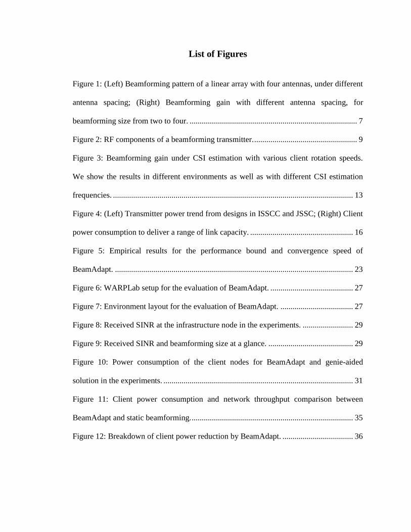
List of Figures

Figure 1: (Left) Beamforming pattern of a linear array with four antennas, under different

antenna spacing; (Right) Beamforming gain with different antenna spacing, for

beamforming size from two to four. ................................................................................... 7

Figure 2: RF components of a beamforming transmitter. ................................................... 9

Figure 3: Beamforming gain under CSI estimation with various client rotation speeds.

We show the results in different environments as well as with different CSI estimation

frequencies. ....................................................................................................................... 13

Figure 4: (Left) Transmitter power trend from designs in ISSCC and JSSC; (Right) Client

power consumption to deliver a range of link capacity. ................................................... 16

Figure 5: Empirical results for the performance bound and convergence speed of

BeamAdapt. ...................................................................................................................... 23

Figure 6: WARPLab setup for the evaluation of BeamAdapt. ......................................... 27

Figure 7: Environment layout for the evaluation of BeamAdapt. .................................... 27

Figure 8: Received SINR at the infrastructure node in the experiments. ......................... 29

Figure 9: Received SINR and beamforming size at a glance. .......................................... 29

Figure 10: Power consumption of the client nodes for BeamAdapt and genie-aided

solution in the experiments. .............................................................................................. 31

Figure 11: Client power consumption and network throughput comparison between

BeamAdapt and static beamforming. ................................................................................ 35

Figure 12: Breakdown of client power reduction by BeamAdapt. ................................... 36

List of Tables

Table 1: Simulation settings for the power tradeoff analysis. ...................................... 16

1

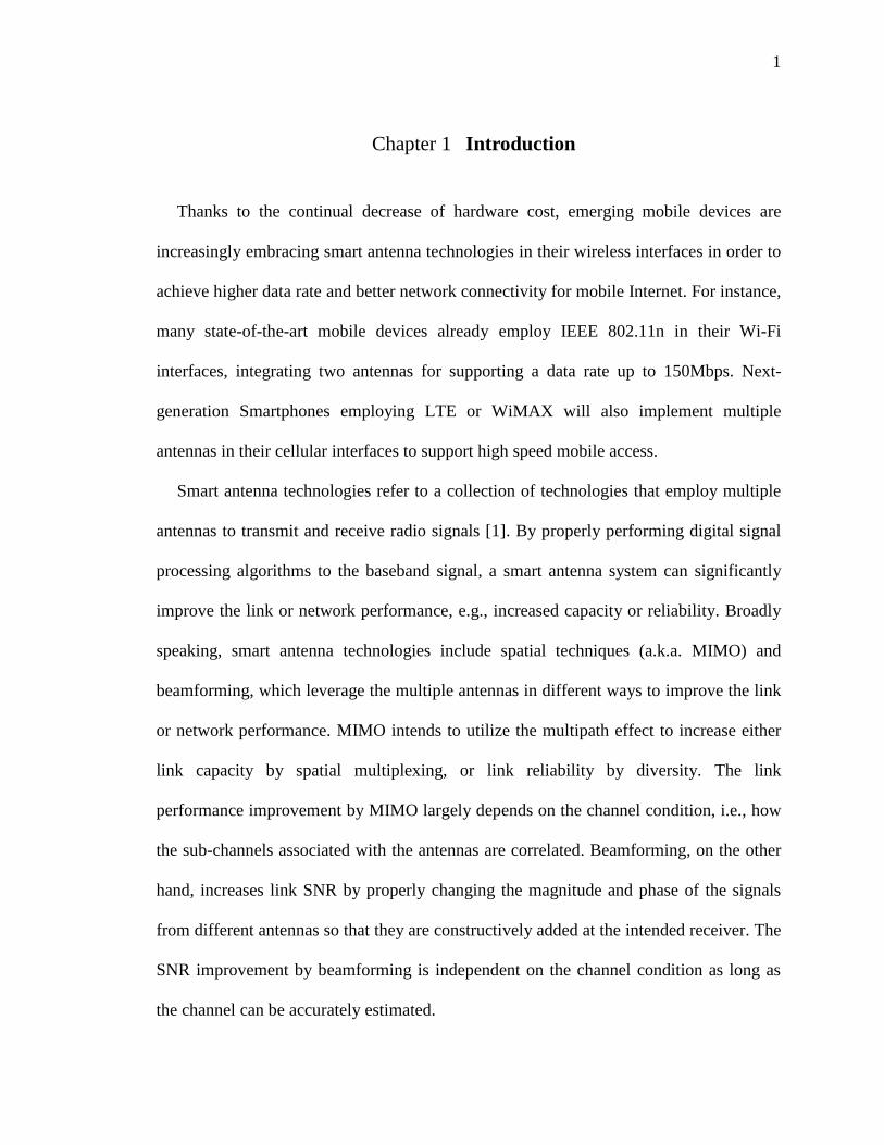
Chapter 1 Introduction

Thanks to the continual decrease of hardware cost, emerging mobile devices are

increasingly embracing smart antenna technologies in their wireless interfaces in order to

achieve higher data rate and better network connectivity for mobile Internet. For instance,

many state-of-the-art mobile devices already employ IEEE 802.11n in their Wi-Fi

interfaces, integrating two antennas for supporting a data rate up to 150Mbps. Next-

generation Smartphones employing LTE or WiMAX will also implement multiple

antennas in their cellular interfaces to support high speed mobile access.

Smart antenna technologies refer to a collection of technologies that employ multiple

antennas to transmit and receive radio signals [1]. By properly performing digital signal

processing algorithms to the baseband signal, a smart antenna system can significantly

improve the link or network performance, e.g., increased capacity or reliability. Broadly

speaking, smart antenna technologies include spatial techniques (a.k.a. MIMO) and

beamforming, which leverage the multiple antennas in different ways to improve the link

or network performance. MIMO intends to utilize the multipath effect to increase either

link capacity by spatial multiplexing, or link reliability by diversity. The link

performance improvement by MIMO largely depends on the channel condition, i.e., how

the sub-channels associated with the antennas are correlated. Beamforming, on the other

hand, increases link SNR by properly changing the magnitude and phase of the signals

from different antennas so that they are constructively added at the intended receiver. The

SNR improvement by beamforming is independent on the channel condition as long as

the channel can be accurately estimated.

2

For a single link, MIMO can increase its capacity by up to N where N is the number of

antennas (number of transmit or receiver antennas, whichever is smaller) [2];

beamforming, however, can only increase the link SNR by up to N [1], which according

to Shannon theory can be translated into a capacity improvement of approximately log(N).

Therefore, in typical mobile environments, with reasonable multipath effect, MIMO is

more likely to be beneficial for a single link in terms of capacity improvement. However,

MIMO has a much higher antenna spacing requirement than beamforming does, making

the implementation of MIMO with a large number of antennas on mobile devices much

more challenging.

Equally crucial is the power overhead of both MIMO and beamforming, by their use

of multiple active RF chains simultaneously. Our parallel work on MIMO, called RF

Chain Management [3], is addressing this power issue by optimizing the tradeoff between

link capacity and end device power efficiency. By minimizing the energy per bit for

either transmission or reception or both, RF Chain Management can on average increase

the device power efficiency by 25% while achieving the required data rate. The

optimization, however, is constrained to a single link.

For our work reported in this thesis, we employ beamforming on mobile devices and

study its optimal use in terms of power efficiency. Our motivation comes from a key

observation towards all current and emerging wireless standards: they assume their

mobile accessing clients are omni directional for transmission. As mentioned above,

while the multiple antennas on clients can be used as MIMO to improve the rate of each

link, we highlight an important fact that current mobile networks are greatly limited by

interference instead of individual link capacity, as the number of mobile devices

3

explodes. As a result, compared to MIMO which attempts to improve link rate,

beamforming is preferably appreciated by current mobile networks to combat with the

interference problem.

While beamforming has been well studied and already deployed for base stations,

access points, and vehicles, it has never been examined for mobile devices due to three

physical challenges of mobile devices: small size, mobility, and limited power. Naturally,

the first question one may ask is: is beamforming feasible for mobile devices? We answer

this question by examining the three challenges. (i) First, we show that single-user

beamforming with two to four antennas can fit into reasonably sized mobile devices with

a linear or circular array. (ii) Second, we experimentally demonstrate that the

beamforming gain remains high even when the device can not only move but also rotate.

(iii) Finally, using data from research prototypes and emerging products, we show that

beamforming can be even more power-efficient than its single antenna counterpart, by

making an increasingly profitable tradeoff between transmit and circuit power. More

importantly, we reveal the existence of the optimal number of active antennas, or the

optimal beamforming size, which minimizes the device overall power. We show that the

optimal beamforming size is dependent on channel condition and required link capacity,

which strongly suggests an adaptive use of beamforming that adjusts the beamforming

size and turns off idle antennas for power efficiency.

Such adaptive beamforming is straightforward to realize for a single link because the

optimal beamforming size can be analytically calculated. However, with multiple

interfering clients, identifying the optimal beamforming size for each client is very

challenging, due to not only the absence of an analytical solution, but also the

4

requirement of client collaboration to enumerate all beamforming size combinations.

Therefore, the second question we seek to answer is: can each client in a large-scale

network individually identify its beamforming size that collectively approaches the

optimal tradeoff with minimum network power consumption? We answer this question by

proposing BeamAdapt, a distributed solution with which each client optimizes its

beamforming size without coordination with others. The key idea of BeamAdapt is

simple: each client iteratively adjusts its beamforming size solely based on the SINR at

its own receiver. We show that BeamAdapt has guaranteed convergence and closely

approaches the optimal.

We evaluate BeamAdapt first through a prototype-based experiment of a two-link

network and then a Qualnet-based simulation of a large-scale network. Our experimental

results show that BeamAdapt consumes only 5% higher power compared to a genie-aided

solution as the performance bound of BeamAdapt in reality. For our Qualnet-based

simulation, we realize BeamAdapt in the context of modern cellular networks. We show

that by cleverly leveraging uplink power control, BeamAdapt can be easily realized on

mobile clients with trivial protocol modification. We show that within a large-scale

cellular network, BeamAdapt with four antennas can reduce power consumption of the

client wireless transceiver by 54% with similar network throughput.

In summary, we make the following technical contributions toward beamforming on

mobile devices:

We report the first feasibility study of beamforming on mobile devices in terms of

form factor, power efficiency, and device mobility.

5

We provide a simple yet effective solution, BeamAdapt that allows each client in

the network to rapidly identify the optimal beamforming size to achieve required

capacity with near-optimal power efficiency. The simplicity of BeamAdapt is

indeed a strength, allowing its immediate realization on cellular mobile devices.

We report a prototype of BeamAdapt based on the WARP platform and a system

design for realizing BeamAdapt in cellular networks.

We note that BeamAdapt can be extended in three important ways. Firstly, while we

propose BeamAdapt for transmit beamforming in this work, receive beamforming on

mobile clients can similarly adopt BeamAdapt for power efficiency, with an even simpler

formulation. Secondly, BeamAdapt is general for any receiver architectures. That

assumed in this work, i.e., treating interference as noise, is in fact an effective

architecture to leverage the benefit of BeamAdapt. Finally, BeamAdapt leverages the

beamforming gain to achieve client power efficiency given the capacity requirement. The

beamforming gain can be reciprocally used to improve the capacity given the client

power constraint, indicating a dual formulation of BeamAdapt.

The rest of the paper is organized as follows. Chapter 2 presents background

knowledge on beamforming. Chapter 3 presents a feasibility study of using beamforming

on mobile devices. Chapter 4 provides the theoretical framework of BeamAdapt. Chapter

5 provides the prototype-based evaluation of BeamAdapt and Chapter 6 offers its

simulation-based counterpart. Chapter 7 addresses related works and Chapter 8 concludes

the paper.

6

Chapter 2 Beamforming Primer

Unlike omni directional transmission with a single antenna, beamforming uses a group

of antennas to increase the SNR of the received signal. Each antenna includes a passive

antenna and a devoted RF chain that bridges the baseband and RF signal. Beamforming

operates by assigning different weights to the baseband signal and then transmitting them

through multiple antennas, or

,

where the baseband signal, weight vector and output signal vector are denoted as s(t), w

and x(t), respectively. The beamforming gain G is defined as the ratio of the received

SNR with beamforming to that with a single antenna. Noticeably, G is dependent on the

number of active antennas, or beamforming size, N.

2.1 Antenna Spacing

Antenna spacing also has a significant impact on the beamforming gain. When the

antenna spacing is sufficient, the maximal beamforming gain, Gmax, is equal to the

beamforming size N [2], or 10log(N) in dB. It is achieved when signals from each

transmit antenna add coherently at the receiver, independent on the direction of the

receiver or the angle of the antenna array relative to the receiver.

When the antenna spacing decreases, the beamforming pattern becomes wider as

shown by Figure 1 (Left), because the angular resolution does not suffice to suppress the

correlation between individual signals. As shown by Figure 1 (Right), when the antenna

spacing drops below certain threshold, the peak beamforming gain will drop due to the

7

Figure 1: (Left) Beamforming pattern of a linear array with four antennas,

under different antenna spacing; (Right) Beamforming gain with different

antenna spacing, for beamforming size from two to four.

30

210

60

240

90

270

120

300

150

330

180 0

0.5lambda

0.3lambda

0.1lambda

0 0.1 0.2 0.3 0.4 0.50

1

2

3

4

5

6

7

Antenna spacing (wavelength)

Peak b

eam

form

ing g

ain

(dB

)

4 antennas

3 antennas

2 antennas

power leakage toward a wider range of directions. The minimum requirement for

maintaining the maximal beamforming gain depends on the number of antennas and is

typically 0.3-0.4λ where λ is the wavelength of the carrier signal.

In this work we only consider single-user beamforming, where the transmitter

optimizes its weight vector for a single receiver [2]. We note that other multi-antenna

techniques typically have more demanding requirement for antenna spacing. Multi-user

beamforming [3] and null beamforming require the antenna spacing be above 0.5λ [4], in

order to exploit additional degrees of freedom when choosing the weight vector. Spatial

multiplexing/diversity techniques, a.k.a. MIMO techniques, typically need an antenna

spacing of multiple wavelengths to operate with a satisfactory capacity improvement [4].

Apparently, they do not fit into iPhone-like mobile devices for the frequency bands in use

today (2 to 5GHz).

8

2.2 Channel Estimation

To guarantee that the signals from multiple transmit antennas add coherently at the

receiver, beamforming requires channel knowledge at the transmitter. In single-user

beamforming, the weight vector is assigned as w=h*, where h is the channel vector with

each of its elements representing the channel coefficient between a transmit antenna and

the receiver. The channel vector h is often denoted as channel state information (CSI).

For transmit beamforming, CSI can be obtained through either closed-loop or open-loop

estimation. For closed-loop estimation, the receiver leverages the training symbols sent

from the transmitter to calculate the channel coefficients and sends it back to the

transmitter. For open-loop CSI estimation, the transmitter estimates the reverse channel

when receiving and uses it for transmitting. Apparently, open-loop CSI estimation

requires channel reciprocity to be effective.

2.3 Power Characteristic

For single-user beamforming, given h, the weight vector w is also given without the

need of any additional computation. This is different to MIMO techniques which often

need considerable signal encoding and processing even at the transmitter. As a result,

single-user beamforming incurs little power overhead by baseband processing and we

next focus on its RF power characteristic. Figure 2 illustrates the major RF hardware

components of a beamforming transmitter. The transmitter consists of multiple RF chains,

each of which is connected to an antenna. When we say an antenna is active, we mean

that the RF chain connected to the antenna is powered on and active. When a

9

Figure 2: RF components of a beamforming transmitter.

FrequencySynthesizer

Baseband Signal

DACFilter Mixer Filter PA1

Baseband Signal

DACFilter

Mixer

Filter PAN

N⋮

PPAPCircuit

PShared

beamforming antenna is not in use, the corresponding RF chain can be powered off to

conserve power.

As shown by Figure 2, the transmitter power consumption can be decomposed into

that of the circuitry shared by all active RF chains, i.e. the frequency synthesizer, denoted

as PShared, and that of each active RF chain. The power contributed by each active RF

chain can be further broken down to that by the power amplifier, and that by the rest of

the chain, denoted as PCircuit. Since we assume identical power amplifiers for all RF

chains, we combine their power consumption, jointly denoted as PPA, with the output

power from transmit antenna included. Clearly, PPA is dependent on the total transmit

power, PTX, while PCircuit is constant irrespective of PTX.

We model PPA as PPA=PTX/η, where η is the efficiency of the power amplifier. The

efficiency η is usually dynamic depending on the transmit power, and here we

approximate η as a linear function of PTX [5] while the power amplifier itself is not linear.

As a result, the total power P can be fairly accurately modeled as

10

(1)

In the rest of the paper, we adopt parameters as follows: ηmin=0.3, ηmax=0.5,

PCircuit=48.2mW, PShared=50mW. They are chosen partially based on [5, 6] as well as all

recent CMOS wireless transceiver designs we have collected (see Section 3.3). Those

parameters are on par with state-of-the-art transceiver designs in 2-5GHz band [7].

11

Chapter 3 Feasibility Study

The first reaction one may have toward beamforming on mobile device is likely to be:

is it feasible at all (possibly thinking of the bulky, power-hungry Phocus Array system

[8])? In this section, we examine the three key physical challenges to put beamforming

on mobile devices: size, mobility, and power efficiency. Our key conclusion after a

careful examination is: beamforming not only is feasible for reasonably sized mobile

devices but also can improve their power efficiency if used properly.

3.1 Form Factor

With the advancement of semiconductor technologies, multiple RF chains are already

being integrated into a single transceiver chip, e.g., [9]. Therefore, the form factor

challenge posed by beamforming only stems from its antenna spacing requirement. As

discussed in Section 2.1, beamforming typically requires the antenna spacing to be higher

than 0.3λ-0.4λ or 4.5cm-6cm in the 2GHz band.

There is no obstacle for medium-size mobile devices such as Tablets and NetBooks to

embrace a beamforming array with fours antennas, in either a linear or a circular array.

Even small-size mobile devices such as iPhone-like Smartphones can accommodate two

antennas in a linear array or four in a circular array. Even if the antenna spacing

requirement cannot be strictly satisfied, the corresponding drop of the beamforming gain

will be approximately linear according to Figure 1, and one can still achieve a significant

gain compared to a single antenna.

12

It is also worth noting that multi-antenna solutions using passive directional antennas

reported in [1] do not have much antenna spacing requirement because only one

directional antenna is active at a time. However, the solution requires all the directional

antennas to be properly oriented, which imposes a different and even larger form factor

challenge.

3.2 Mobility

A mobile device can not only move but also rotate. Recent work has shown that

beamforming with predefined beam patterns can cope with vehicular mobility very well,

e.g., [10, 11]. However, real-time beamforming poses a new challenge due to the

requirement of accurate CSI, including only not the magnitude but also the phase of the

channel coefficients which are largely affected by device rotation. Therefore, next we

focus on evaluating the beamforming gain under device rotation since device rotation can

potentially introduce faster channel variation than mobility can.

We perform the experiments using the WARP software radios [12]. We build a

circular array with four antennas on one WARP board as the mobile client, and use a

single antenna at the other WARP board as the infrastructure node. The client and

infrastructure nodes are placed close to the allowed range with a moderate SNR (5dB),

i.e. 10 meters in our experiments. The client node continuously sends training symbols to

the infrastructure node every 10ms and the latter sends back the estimated CSI through an

Ethernet cable. Therefore, the mobile client updates the CSI each 10ms, calculates the

weight vector and forms a beam. To challenge the CSI estimation, we rotate the client

node with a computerized motor at 90°/s and 180°/s respectively, while realistic mobile

13

(a) CSI estimation per 10ms

(b) CSI estimation per 100ms

Figure 3: Beamforming gain under CSI estimation with various client rotation

speeds. We show the results in different environments as well as with different

CSI estimation frequencies.

N=2 N=40

3

6

Beam

form

ing g

ain

(dB

)

Indoor

Max

Static

90d/s

180d/s

N=2 N=40

3

6

Beam

form

ing g

ain

(dB

)

Outdoor

Max

Static

90d/s

180d/s

N=2 N=40

3

6

Beam

form

ing g

ain

(dB

)

Indoor

Max

Static

90d/s

180d/s

N=2 N=40

3

6

Beam

form

ing g

ain

(dB

)

Outdoor

Max

Static

90d/s

180d/s

devices rotate at a much slower speed, e.g. 10°/s as the median and 120°/s as the upper

bound [1]. We repeat the experiments both indoor and outdoor. While we could not

simultaneously examine different beamforming sizes and different CSI estimation

frequencies in real time, we have collected traces of the channel coefficients and emulate

the channel offline. That is, we replay the channel using the recorded traces but assume

different beamforming sizes (2 and 4), and different CSI estimation frequencies (10ms

14

and 100ms). Since the beamforming gain is only dependent on the CSI, the offline

emulation gives identical results as real-time evaluation does.

The key question we aim to answer is: what is the impact of device rotation on CSI

estimation and corresponding beamforming gain? To see this, Figure 3 shows the

average beamforming gain under CSI estimation with different rotation speeds of the

client. In each sub-figure of Figure 3, four values of beamforming gain for each

beamforming size are shown: the upper bound given by perfect CSI (Max), the one given

by estimated CSI with stationary client (Static), the one given by estimated CSI with

rotating client at 90°/s (90d/s), and the one given by estimated CSI with rotating client at

180°/s (180d/s).

When the CSI estimation interval is 10ms, the CSI can be very accurate even with

client rotational speed of 180°/s. As a result, the maximal beamforming gain, i.e. 3dB and

6dB with N=2 and N=4 respectively, can be achieved. When the interval is increased to

100ms, the beamforming gain will be affected by client rotation. The rotation has higher

impact for larger beamforming sizes due to a more focused beamforming pattern.

Therefore, we conclude that even under high speed device rotation such as 180°/s,

beamforming can still be effective with reasonable CSI estimation intervals, e.g., 10ms.

In contrast, the solution in [1] achieves a much lower gain relative to the maximal

allowed by the passive directional, e.g. 3dB using 5dBi and 8dBi antennas. Finally, we

observe that the performance of CSI estimation is more stable indoor, due to richer

multipath effect to compensate bad directions. This can be seen from the range of the

beamforming gain in each sub-figure.

15

3.3 Power Efficiency

Although single-user beamforming incurs negligible power overhead in baseband

processing, it increases the power of RF circuitry by simultaneously using multiple active

RF chains compared to a single antenna. While RF integrated circuits improve slower

than their digital counterparts, their power efficiency still improves significantly over

years. To illustrate this trend, we have examined the CMOS wireless transceiver

realizations reported in ISSCC [13] and JSSC [14], the top conference and journal for

semiconductor circuits, from 2003 to 2010, and show their circuit power consumption,

PCircuit+PShared, in Figure 4 (Left). The figure clearly shows the continuous improvement

in the power efficiency of both SISO and MIMO transceivers. As semiconductor process

technologies continue to improve, PCircuit and PShared will continue decreasing. As a result,

PPA will increasingly dominate the total power consumption.

By focusing the transmit power toward the intended direction, beamforming can

reduce PTX and PPA and therefore even improve the power efficiency. Clearly,

beamforming makes a tradeoff between transmit and circuit power: with a beamforming

size of N, the transmit power can be reduced to 1/N compared to a single antenna due to

the beamforming gain. Note that beamforming is able to yield a total transmit power

reduction instead of that of each antenna, i.e. the reduction is not because of the

allocation of transmit power into multiple antennas.

16

Figure 4: (Left) Transmitter power trend from designs in ISSCC and JSSC;

(Right) Client power consumption to deliver a range of link capacity.

Table 1: Simulation settings for the power tradeoff analysis.

Parameters Values

Distance

Max beamforming size

0.5km

4

Power decay factor 4

Receiver noise

Channel bandwidth

Carrier frequency

-170dBm/Hz

5MHz

2GHz

2002 2004 2006 2008 20100

200

400

600

800

1000

1200

Year

Tra

nsm

itte

r P

ow

er

Consum

ption (

mW

)

SISO

2x2 MIMO

2 4 60

200

400

600

800

1000

1200

Clie

nt pow

er

consum

ption (

mW

)

Uplink capacity (b/s/Hz)

N=1

N=2

N=3

N=4

We next briefly analyze this tradeoff between transmit and circuit power. For

simplicity, we consider a single uplink channel from a mobile client to its infrastructure

node and assume line-of-sight (LOS) propagation and the settings specified in Table 1.

Figure 4 (Right) shows the client power consumption calculated by Equation (1) to

deliver a range of link capacity for beamforming sizes from one to four. One can make

two important conclusions from the figure. (i) First, beamforming (N>1) is already more

efficient than omni directional transmission (N=1) when delivering a capacity of

17

3.2b/s/Hz or higher. (ii) Second, the larger the required link capacity, the larger the most

power efficient beamforming size. This shows that beamforming is increasingly desirable

in delivering higher capacity.

18

Chapter 4 Adaptive Beamforming on Mobile Devices

The above findings above suggest an adaptive beamforming system that adjusts the

beamforming size for the optimal tradeoff between transmit and circuit power, according

to link capacity requirement. Next we show that to achieve the best tradeoff in a network

is indeed non-trivial and, therefore, provide a simple yet effective solution, BeamAdapt.

4.1 Key Tradeoff and Challenge

As shown above, the optimal beamforming size varies according to the required link

capacity. Given the transmit power decay factor and distance, one can derive the required

transmit power for omni directional transmission, PO, to achieve certain link capacity.

Using Equation (1), we can calculate the optimal beamforming size as

(2)

where C1 and C2 are constants determined by the power amplifier. Again, beamforming

with more antennas is increasingly more efficient as PCircuit decreases according to the

continual progress in semiconductor technologies.

While the optimal tradeoff given by Nopt appears straightforward to identify with a

single link (PO is uniquely decided by the required capacity or SNR), it is challenging to

determine in a network with multiple links. This is because PO is determined by SINR

instead of SNR due to interference. Meanwhile, different beamforming sizes will

generate different interference toward other receivers, implicitly impacting their own

SINR. As a result, the optimal beamforming size can no longer be calculated by Equation

(2).

19

Nonetheless, the tradeoff between transmit and circuit power is still valid and there

exists a most power efficient beamforming size for each client that collectively minimizes

the aggregated client power consumption, or network power consumption. The immediate

question we seek to answer is: how could clients of a large network identify their most

power-efficient beamforming sizes that collectively lead to the minimum network power

consumption?

4.2 Problem Formulation

Since we are interested in client power efficiency, we seek to minimize PNetwork, the

aggregated power consumption by all clients in a network, with a constraint that the

capacity, or equivalently the SINR of each link i, SINRi, must be equal to certain target

value, . The reason of separately constraining individual links is that different links

usually have different capacity requirements. In addition, the beamforming size Ni must

be integers no greater than Ni,max, where Ni,max is the maximum number of antennas on

client i.

Therefore, we formulate the optimization problem as:

where is the power consumption of client i and

.

Solving the above optimization problem is very challenging. Firstly, each of the SINR

constraints is a function of all 2M optimization variables. The SINR function is non-

convex with respect to these variables, yielding the non-convexity of the problem.

20

Secondly, there is no closed-form formulation of the beamforming gain G to unintended

receivers as a function of N. Its dependence on the receiver direction makes low-order

approximation hardly possible. Finally, the integer constraint on Ni renders a NP-hard

mixed integer programming (MIP) problem [15]. While an exhaustive search algorithm

can ultimately offer the solution, the complexity can be as high as ,

which becomes prohibitively complex as M grows. Most importantly, such a brute-force

algorithm requires all the clients have knowledge of each others’ actions in order to

enumerate all beamforming size combinations, and cooperatively choose their

beamforming sizes.

To tackle this problem, we introduce BeamAdapt, a simple yet effective algorithm that

works in a distributed manner: each client simply performs individual optimization on the

beamforming size without cooperation.

4.3 Distributed Algorithm: BeamAdapt

First we decompose the problem into multiple, individual sub-problems, i.e., the ith

link’s problem (i=1,2, M) is

.

The optimal (PTX,i, Ni) is determined iteratively. Let us temporally omit the subscript

below since all clients employ the same algorithm. We assume the transmit power and

beamforming size are

and N(k-1)

for the (k-1)th iteration, and the received SINR is

, then for the kth iteration,

and N(k-1)

are updated by solving the following

optimization problem:

21

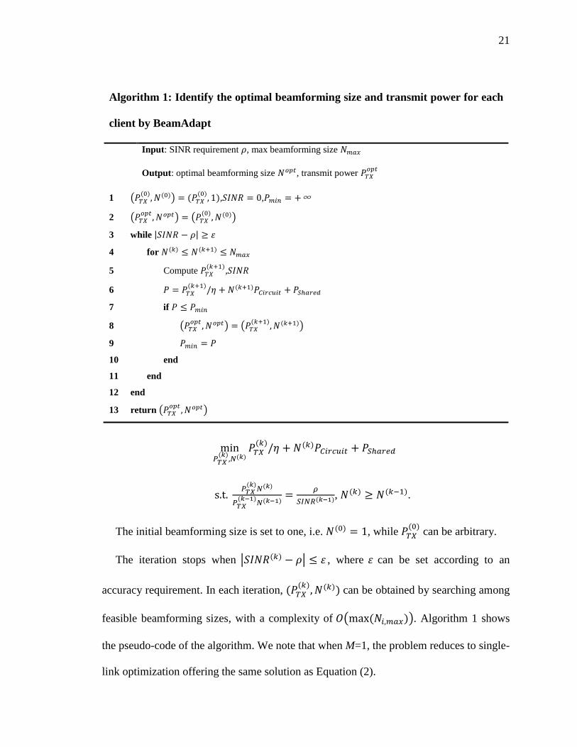
Algorithm 1: Identify the optimal beamforming size and transmit power for each

client by BeamAdapt

Input: SINR requirement , max beamforming size

Output: optimal beamforming size , transmit power

1

, ,

2

3 while

4 for

5 Compute

,

6

7 if

8

9

10 end

11 end

12 end

13 return

, .

The initial beamforming size is set to one, i.e. , while

can be arbitrary.

The iteration stops when , where can be set according to an

accuracy requirement. In each iteration,

can be obtained by searching among

feasible beamforming sizes, with a complexity of . Algorithm 1 shows

the pseudo-code of the algorithm. We note that when M=1, the problem reduces to single-

link optimization offering the same solution as Equation (2).

22

4.4 Convergence of BeamAdapt

The iteration process of BeamAdapt is guaranteed to converge. Next we provide a

brief yet sufficiently illustrative proof. The two key facts we leverage are: (i) whenever

the beamforming sizes are fixed, the iteration of BeamAdapt is isomorphic to a

distributed power control algorithm [16] that ensures convergence; and (ii) the change of

the beamforming size N of each client is monotonous. That is, the beamforming size can

only increase during iteration.

Therefore, we divide the iteration process into multiple stages, , where

during each stage N is constant and only PTX changes. The current stage evolves into

when N changes for any one link. Based on the monotonicity of N we have the

following inequality

,

which indicates a finite number (L) of stages.

During each stage, the beamforming size is fixed; therefore the original problem turns

in to

, .

This problem is isomorphic to the power control problem where a distributed algorithm

ensures convergence [16]. As a result, during each stage ( ) the power control

component either converges, or it moves onto a new stage. Since the number of potential

stages L is finite, the overall algorithm is guaranteed to converge.

4.5 Performance Bound of BeamAdapt

23

(a) Network configuration

(b) Network power comparison

(c) CDF of the additional power

consumption by BeamAdapt

(d) PDF of the convergence speed

of BeamAdapt

Figure 5: Empirical results for the performance bound and convergence speed of

BeamAdapt.

Link 1

Link 2

Link 3

Link 4

Link 5

Link 7

Link 6

0 5 10 15 200

2000

4000

6000

8000

Simulation repetition

Netw

ork

pow

er

consum

ption (

mW

)

BeamAdapt

Bound

Omni

0 0.5 1 1.5 20

0.2

0.4

0.6

0.8

1

Addtional network power consumption (%)

CD

F

2 4 6 80

10

20

30

40

50

60

Number of iterations before convergence

Pro

bability (

%)

We next investigate how fast BeamAdapt converges and how good its steady-state

performance is. It is possible that BeamAdapt converges to a sub-optimal solution.

Unfortunately, the performance bound of BeamAdapt is not analytically obtainable, again

due to the non-convexity of the optimization problem and the integer constraints on the

beamforming size. Therefore, we have to rely on empirical methods to study the

performance bound. We employ a seven-cell network as a first-order approximation of a

24

large-scale infrastructure network as shown in Figure 5 (a): we assume seven

infrastructure nodes are evenly distributed in the space. Other settings are similarly

adopted from

Table 1. To eliminate the dependency of BeamAdapt on the client location, we repeat

the simulation extensively with random locations of the clients. Therefore, we are in fact

averaging the performance of BeamAdapt with various network configurations.

Figure 5 (b) shows a few samples of the network power consumption of BeamAdapt,

and its upper bound given by the theoretically optimal solution using a brute-force

algorithm with client cooperation. The figure also shows the performance of omni for

comparison. Clearly, the performance of BeamAdapt is very close to the optimal and

much better than that of omni. Figure 5 (c) shows the CDF of the additional network

power consumption by BeamAdapt compared to its bound: BeamAdapt indeed converges

to the optimal solution with a probability of 55%, and only incurs 0.5% additional power

compared to the optimal solution when it converges to a sub-optimal.

Using the same network configuration, we can also evaluate the convergence speed of

BeamAdapt, with Figure 5 (d) showing the PDF of the number of iterations to achieve a

small , i.e., 0.1% in our simulation. Clearly, BeamAdapt often converges rapidly, i.e.

with typically less than three iterations to get a stable SINR.

25

Chapter 5 Prototype-based Evaluation

In Chapter 3.2 we experimentally showed the feasibility of beamforming on mobile

devices with a close-to-maximum beamforming gain even when the mobile client rotates

at 180°/s. However, compared to static beamforming with a fixed number of active

antennas, BeamAdapt faces a new challenge due to its iterative nature: are mobile clients

with BeamAdapt able to timely identify the right number of antennas and transmit power

in real-time so that the required SINR is achieved with maximal power reduction? To

answer the question, we use WARP to experimentally evaluate the feasibility of

BeamAdapt in realistic environments.

We must note that BeamAdapt is a general technique compatible with any

infrastructure network architecture such as WLAN or cellular. Since we are not able to

conduct experiments on cellular bands due to the lack of license, we use ISM band

(2.4GHz) to validate the feasibility of BeamAdapt. Our Qualnet-based evaluation in

Section 6, however, will complementarily show the power saving and network

throughput performance of BeamAdapt within a large-scale cellular network.

5.1 BeamAdapt Prototype

We realize BeamAdapt using WARPLab, a framework that facilitates rapid

prototyping of physical layer designs and algorithms. WARPLab allows symbol-level

access to the wireless transceivers embedded on the WARP board, which we leverage to

realize the key functionalities of BeamAdapt including beamforming, transmit power and

beamforming size adaptation, and SINR measurement. In WARPLab, all WARP nodes

26

are connected through an Ethernet router and a laptop with MATLAB interface is used to

control the nodes, implement the algorithm and collect the data.

We have built two types of WARP nodes: one with four antennas implementing

BeamAdapt as the mobile client node and the other with a single antenna as the

infrastructure node. Since we assume the simplest receiver architecture for BeamAdapt,

i.e. treating interference as noise, the performance of BeamAdapt is independent on the

number of antennas on the infrastructure node. The physical wireless channel is assumed

as the uplink channel from client node to infrastructure node, while an Ethernet cable is

used to emulate the downlink channel. Since we are only interested in client transmission

(uplink channel), we generate dummy frames only at the client node and continuously

send them to the infrastructure node.

5.2 Experiment Setup

We test the prototype under two physical environments: one inside an office building

and the other on an empty lawn, both in a university campus. The former represents a

typical indoor environment while the latter outdoor. We use four WARP nodes, including

two client nodes and two infrastructure nodes, to form a two-link network. Figure 6

shows our setup using WARPLab and Figure 7 shows the locations of the client and

infrastructure nodes.

27

Figure 6: WARPLab setup for the evaluation of BeamAdapt.

Figure 7: Environment layout for the evaluation of BeamAdapt.

Laptop with MATLAB

Ethernet Router

Infrastructure Node 1 Infrastructure Node 2

Client Node 1 Client Node 2

Uplink(Wireless)

Uplink(Wireless)

Client (Indoor)

Infrastructure (Indoor)

Client (Outdoor)

Infrastructure (Outdoor) 5m

While in realistic wireless networks there might be more links that interfere with each

other, we consider this two-link network as a reasonable setup for experiments. Firstly,

the two-link network is a widely used model in wireless network researches [4], due to its

simplicity and generality. Secondly, even though in realistic such as cellular networks

there are more than two base stations within the coverage of a mobile client, the client is

often mainly interfering with only one additional base station, due to the distributed

28

fashion of placing base stations in a certain area and that each client often connects to the

closest base station. Finally, since we have selected the ISM bands and the environments

of our experiments have continuous but unpredictable wireless transmissions, there are

indeed other interference sources at the infrastructure nodes.

In our experiments, we add both movement and rotation to the two client nodes, by

manually moving and rotating them. The rotation speed is from zero to one hundred

twenty degrees per second, consistent with [1]. The movement is about zero to one meter

per second. Due to the limitation of WARPLab that the WARP boards have to be

connected by Ethernet cables, we can only add pedestrian movement speed in the

experiment but will simulate a much higher speed in the Qualnet simulation in Chapter 6.

5.3 Experimental Findings

We examine the effectiveness of BeamAdapt in realistic environments with two key

metrics, received SINR at the infrastructure node and power consumption by the client

node. Apparently, they jointly represent the key functionality of BeamAdapt according to

our formulation in Section Chapter 4. For received SINR, we examine whether

BeamAdapt can closely approach the required SINR even with iteration and client

mobility. For power consumption, we compare the power consumption of BeamAdapt

with a genie-aided solution which can always correctly pick the right beamforming size

and transmit power without the need of iteration. Clearly, the genie-aided solution can

achieve maximal power reduction. To realize the comparison, we recorded traces the

channel coefficients during all our measurements and replayed the channel offline to

emulate the genie-aided solution.

29

Figure 8: Received SINR at the infrastructure node in the experiments.

Figure 9: Received SINR and beamforming size at a glance.

I/S I/M O/S O/M0

2

4

6

8

10

SIN

R (

dB

)

5dB

Client Node 1

Client Node 2

I/S I/M O/S O/M0

5

10

15

SIN

R (

dB

)

8dB

Client Node 1

Client Node 2

0 5 10-10

0

10

20

SIN

R (

dB

)

Time (s)

Client Node 1

0 5 101

2

3

4

Beam

form

ing s

ize

Time (s)

0 5 10-10

0

10

20

SIN

R (

dB

)

Time (s)

Client Node 2

0 5 101

2

3

4

Beam

form

ing s

ize

Time (s)

5.3.1 Received SINR

We first report the received SINR at the infrastructure nodes. To maximally leverage

the range of WARP nodes without losing generality, we assume moderate SINR, e.g. 5dB

and 8dB as the constraint. Figure 8 shows the mean and variance of the received SINR at

the two infrastructure nodes, for four scenarios: Indoor/Static (I/S), Indoor/Mobile (I/M),

Outdoor/Static (O/S), and Outdoor/Mobile (O/M).

We report two key findings from the figure. (i) First, on average BeamAdapt can

closely approach the required SINR, i.e. 5dB and 8dB respectively, for both stationary

and mobile client nodes. In most of the scenarios the standard variance is below 3dB,

30

meaning that the BeamAdapt iteration does not render significant SINR deviation from

the target value. (ii) Second, in the outdoor/mobile scenario BeamAdapt yields much

higher variance of the received SINR. This is consistent to our observation of the

beamforming gain in Section 3.2, due to the lack of compensation by multi-path effect to

the out-of-dated channel and beamforming size.

Figure 9 shows a ten-second snapshot of the received SINR as well as the

beamforming size of two infrastructure nodes. Clearly, most of the time BeamAdapt is

able to timely cope with channel variation and achieves a stable SINR, while the

beamforming size is indeed being adapted. We have chosen the Indoor/Mobile scenario

to show in the figure while the other scenarios exhibit similar characteristics, as

demonstrated by Figure 8

While BeamAdapt on average achieves the required SINR, it does not guarantee that

the SINR is above the target value. This is due to the formulation of BeamAdapt that

seeks to use the exact amount of power to achieve certain capacity. Nonetheless,

BeamAdapt will not lead to a large outage probability, since one can simply leave a SINR

margin and set the required SINR in BeamAdapt a bit higher than the actual intended

value. For example, if a SINR of 5dB is needed, one can set 8dB as the constraint in

BeamAdapt and it will maintain the SINR above the threshold with a probability of 87%

according to our results.

5.3.2 Power Consumption

We next compare the power consumption of BeamAdapt with that of the genie-aided

solution. It is important to highlight that given the transmit power and beamforming size,

31

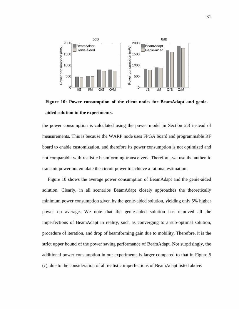
Figure 10: Power consumption of the client nodes for BeamAdapt and genie-

aided solution in the experiments.

I/S I/M O/S O/M0

500

1000

1500

2000

Pow

er

consum

ption (

mW

)

5dB

BeamAdapt

Genie-aided

I/S I/M O/S O/M0

500

1000

1500

2000

Pow

er

consum

ption (

mW

)

8dB

BeamAdapt

Genie-aided

the power consumption is calculated using the power model in Section 2.3 instead of

measurements. This is because the WARP node uses FPGA board and programmable RF

board to enable customization, and therefore its power consumption is not optimized and

not comparable with realistic beamforming transceivers. Therefore, we use the authentic

transmit power but emulate the circuit power to achieve a rational estimation.

Figure 10 shows the average power consumption of BeamAdapt and the genie-aided

solution. Clearly, in all scenarios BeamAdapt closely approaches the theoretically

minimum power consumption given by the genie-aided solution, yielding only 5% higher

power on average. We note that the genie-aided solution has removed all the

imperfections of BeamAdapt in reality, such as converging to a sub-optimal solution,

procedure of iteration, and drop of beamforming gain due to mobility. Therefore, it is the

strict upper bound of the power saving performance of BeamAdapt. Not surprisingly, the

additional power consumption in our experiments is larger compared to that in Figure 5

(c), due to the consideration of all realistic imperfections of BeamAdapt listed above.

32

Chapter 6 Evaluation of BeamAdapt in Cellular Networks

To complement the prototype-based evaluation, we next use simulation to evaluate

BeamAdapt with a large-scale network. To achieve a close-to-reality evaluation, we

adopt current cellular protocols and introduce a system design of BeamAdapt that is

realizable with trivial protocol modification. We employ the simulation tool Qualnet [17]

for its open-source feature and support of cellular protocols.

6.1 Cellular-based System Design

We realize BeamAdapt in the mobile accessing clients in a cellular network and again

focus on uplink transmission. Due to its distributed property, BeamAdapt relieves clients

in the network from inter-client cooperation thereby entails minor protocol modification.

There are two key concerns regarding the system realization of BeamAdapt. First, how

does BeamAdapt perform uplink CSI estimation? Second, how does BeamAdapt obtain

the received SINR to perform the beamforming size adaptation? We next answer them

below.

6.1.1 Uplink CSI Estimation

Due to the absence of uplink/downlink channel reciprocity in cellular network [18],

we can only adopt closed-loop CSI estimation in BeamAdapt (see Section 2.2). That is,

the client concatenates a short field made up of several training symbols to the data field

in each uplink frame. Seeing the training symbols, the base station estimates uplink CSI

and sends it back to the client. Thanks to the full-duplex property of cellular channels, the

estimated CSI can be simultaneously delivered to the client through downlink control

33

signaling while the client is involved in uplink transmission. Therefore, CSI feedback

does not incur any additional uplink channel occupation. Moreover, the training field can

be very short compared to the entire frame, i.e. a 16μs training field for beamforming size

of four and a 10ms frame in UMTS and LTE [18], which further render the overhead of

CSI estimation negligible. According to our measurement in Chapter 3.2, the 10ms frame

length in UMTS/LTE guarantees accurate CSI estimation of BeamAdapt, even with client

rotation.

6.1.2 Beam Adaptation

To adapt the beamforming size and transmit power, BeamAdapt needs to know the

received SINR of each frame. While it can be similarly sent back to the client through

downlink control signaling, we seek to minimize the protocol modification, by leveraging

the uplink power control mechanism inherent in cellular protocols. Uplink power control

is widely used in cellular protocols to maintain a constant SINR of each client at the base

station. It is initiated by the base station, through sending a power control command to

the client, containing the value of required transmit power. Noticeably, this required

transmit power is actually PO in Equation (2), and one can directly identify the optimal

transmit power PTX and beamforming size N using PO, as one iteration in the BeamAdapt

algorithm. This way, the received SINR is no longer needed and no protocol changed is

required.

6.2 Simulation Setup

Since the beamforming hardware is not included in Qualnet, we have to virtually

realize a beamforming system on the client by generating dynamic beamforming patterns

34

in real-time and adopting the power model in Section 2.3 to calculate client power

consumption.

We use the same network configuration shown in Figure 5 (a), and assume the UMTS

protocol in Qualnet. However, here we add more clients, i.e. thirty, to mimic realistic

base station scheduling and handoff in cellular networks. The area is 4km×4km and the

base stations have fixed locations, 1.5km from its neighbors. While the range of each

base station is approximately 1km, we let their coverage overlap similar to realistic

cellular networks in urban areas. The clients are allowed to have movement with random

speed from zero to seventy miles per hour, corresponding to a wide range of client

movement speed such as stationary, pedestrian and vehicular. We also incorporate client

rotation with an upper bounded speed of 120°/s [1]. We add two applications to the

client: FTP with an unlimited-size file to transfer and constant-bit-rate (CBR) with

multiple relatively small packets. FTP generates continuous traffic. CBR, on the contrary,

creates intermittent traffic by the idle intervals between the small-size packets. Therefore,

the FTP traffic has a higher capacity requirement than the CBR traffic.

We evaluate the power reduction benefit of BeamAdapt by comparing it with omni

directional transmission and static beamforming with a fixed beamforming size. We

examine BeamAdapt and static beamforming (BF) with two, four and eight antennas.

Note that BeamAdapt with N=4 means that the client can select from one to four active

antennas (with unused antennas powered off) while BF with N=4 always uses four active

antennas.

6.3 Findings

35

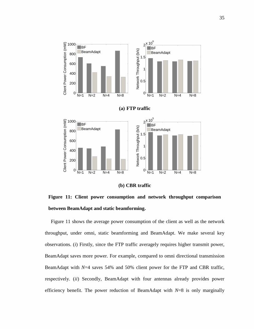
(a) FTP traffic

(b) CBR traffic

Figure 11: Client power consumption and network throughput comparison

between BeamAdapt and static beamforming.

N=1 N=2 N=4 N=80

200

400

600

800

1000

Clie

nt P

ow

er

Consum

ption (

mW

)

BF

BeamAdapt

N=1 N=2 N=4 N=80

0.5

1

1.5

2x 10

6

Netw

ork

Thro

ughput (b

/s)

BF

BeamAdapt

N=1 N=2 N=4 N=80

200

400

600

800

1000

Clie

nt P

ow

er

Consum

ption (

mW

)

BF

BeamAdapt

N=1 N=2 N=4 N=80

0.5

1

1.5

2x 10

5

Netw

ork

Thro

ughput (b

/s)

BF

BeamAdapt

Figure 11 shows the average power consumption of the client as well as the network

throughput, under omni, static beamforming and BeamAdapt. We make several key

observations. (i) Firstly, since the FTP traffic averagely requires higher transmit power,

BeamAdapt saves more power. For example, compared to omni directional transmission

BeamAdapt with N=4 saves 54% and 50% client power for the FTP and CBR traffic,

respectively. (ii) Secondly, BeamAdapt with four antennas already provides power

efficiency benefit. The power reduction of BeamAdapt with N=8 is only marginally

36

Figure 12: Breakdown of client power reduction by BeamAdapt.

0.15 0.3 0.45 0.6 0.750

10

20

30

40

50

60

70

80

Distance between client and BS (km)

Client pow

er

reduction (

%)

TX power reduction only

Int reduction only

0.15 0.3 0.45 0.6 0.750

10

20

30

40

50

60

70

80

Distance between client and BS (km)

Client pow

er

reduction (

%)

TX power reduction only

Int reduction only

better than that of BeamAdapt with N=4. This is due to the confined range of cellular

radio signal and the corresponding maximal transmit power limit. (iii) Finally, the

network throughput achieved by BeamAdapt is only slightly lower (<5%) than that by

omni directional transmission, and is as good as that by their respective static

beamforming counterparts. The slight degradation is due to client mobility and thereby

the drop of the beamforming gain, similar to what we observed in Chapter 3.2.

We also note that the power reduction by BeamAdapt stems from two benefits of

beamforming: the improvement of SNR and the reduction of interference. Qualnet

simulation allows us to further examine the power saving contribution from these two

benefits. That is, we first only keep the transmit power reduction capability of

BeamAdapt and then the interference reduction capability only. Figure 12 shows their

respective contribution to client power reduction, with different distance from the client

to the base station. Clearly, as the client moves to cell boundary, i.e. with a larger

distance to the base station, both capabilities can save more power, and they collectively

achieve a higher overall power reduction of the client. This is because when the client is

37

approaching cell boundary, only not the required transmit power increases, but also the

interference between adjacent cells is more severe.

38

Chapter 7 Related Work

Our work is the first that aims to enable real-time and power efficient beamforming on

mobile devices. Nonetheless, multi-antenna techniques and directional communication

have been generally studied in many other regimes. We next discuss related work.

7.1 Beamforming

No existing work on beamforming has considered and optimized its use on mobile

devices such as Tablets and smartphones. Recent work such as [10, 11] considered using

beamforming on vehicles to enhance the uplink connection as the client moves. The

authors of [19] have experimentally shown the effectiveness of switched beam systems in

indoor environments. However, all of above solutions use the Phocus Array system [8]

and none supports real-time beamforming. More importantly, these solutions do not

consider dynamic number of active antennas in beamforming and its power efficiency

benefit.

7.2 Directional Antennas on Mobile Devices

Passive directional antenna is an efficient yet inflexible way to realize directional

communication. Many have studied them for infrastructure nodes and mobile nodes that

do not rotate, e.g. see [20-27]. Most of the authors focus on MAC protocol designs. In

contrast, BeamAdapt is in the PHY layer and is complementary to directional MAC

designs. Only very recently, the authors of [1, 28] demonstrated the effectiveness of

passive directional antennas in improving transmission throughput and power efficiency

of mobile devices that can rotate like Smartphones. The solution is based on selecting one

39

out of multiple fixed passive directional antennas. However, there is a key limitation

toward their solution: only a limited number of passive antennas are allowed to be

implemented, e.g. four in [1], and they are hard to be properly oriented. Such limitation

renders a confined gain of their solution due to failure to cover all directions, i.e. only

3dB gain using 5dBi and 8dBi antennas. In contrast, beamforming with BeamAdapt can

easily track channel variation and achieves a guaranteed gain of 6dB using four antennas.

7.3 Power Efficient MIMO

While in this work we consider beamforming for its adaptive use in a power efficient

manner, similar concept can be extended to MIMO systems. The authors of [29] have

provided a system design of an adaptive MIMO system and experimentally shown that it

can minimize the energy per bit of the MIMO transceiver by properly choosing the

number of active RF chains. The idea is also explored by the authors of [30] and [31].

The authors of [32] have analytically showed the effectiveness and performance of such

adaptive MIMO systems. These solutions, however, are limited to a single link, while

BeamAdapt is solving a network problem by optimizing the use of beamforming on

multiple mobile clients.

40

Chapter 8 Conclusion

In this work, we reported a first study of beamforming on mobile devices. With both

experiments and data from industry, we showed that beamforming is not only feasible but

also power efficient to mobile devices. We then addressed the challenge of identifying

the optimal use of beamforming on mobile device by formulating an optimization

problem and providing the BeamAdapt solution. Through both experiments and

simulation, we showed that BeamAdapt is able to react to client mobility by promptly

identifying the right beamforming size and the transmit power. Collectively it achieves

more than 50% power reduction of the clients in a large-scale network.

Client directionality through beamforming is a radical departure from omni

directionality assumed by current mobile network paradigms. While we are able to

demonstrate its benefit in client efficiency, more research at various layers of the network

system is required to fully appreciate its potential, which we leave to future work.

41

REFERENCE

[1] T. Sarkar, Smart antennas: Wiley-Interscience Hoboken, NJ, 2003.

[2] A. J. Paulraj, D. A. Gore, R. U. Nabar, and H. Bolcskei, "An Overview of MIMO

Communications—A Key to Gigabit Wireless," Proc. IEEE, vol. 92, pp. 198-218,

2004.

[3] H. Yu, L. Zhong, and A. Sabharwal, "Adaptive RF chain management for energy-

efficient spatial-multiplexing MIMO transmission," in Proc. ACM/IEEE Int.

Symp. Low Power Electronics and Design San Fancisco, CA, USA: ACM, 2009.

[4] L. C. Godara, Smart Antennas: CRC Press, 2004.

[5] M. Blanco, R. Kokku, K. Ramachandran, S. Rangarajan, and K. Sundaresan, "On

the Effectiveness of Switched Beam Antennas in Indoor Environments," in

Passive and Active Network Measurement, 2008, pp. 122-131.

[6] X. Liu, A. Sheth, M. Kaminsky, K. Papagiannaki, S. Seshan, and P. Steenkiste,

"DIRC: increasing indoor wireless capacity using directional antennas," in Proc.

SIGCOMM Barcelona, Spain: ACM, 2009.

[7] V. Navda, A. P. Subramanian, K. Dhanasekaran, A. Timm-Giel, and S. Das,

"MobiSteer: using steerable beam directional antenna for vehicular network

access," in Proc. Int. Conf. Mobile Systems, Applications and Services (MobiSys),

2007, pp. 192-205.

[8] K. Ramachandran, R. Kokku, K. Sundaresan, M. Gruteser, and S. Rangarajan,

"R2D2: regulating beam shape and rate as directionality meets diversity," in Proc.

MobiSys Poland: ACM, 2009.

42

[9] D. G. Rahn, M. S. Cavin, F. F. Dai, N. H. W. Fong, R. Griffith, J. Macedo, A. D.

Moore, J. W. M. Rogers, and M. Toner, "A fully integrated multiband MIMO

WLAN transceiver RFIC," IEEE Journal of Solid-State Circuits, vol. 40, pp.

1629-1641, 2005.

[10] S. Cui, A. J. Goldsmith, and A. Bahai, "Energy-efficiency of MIMO and

cooperative MIMO techniques in sensor networks," IEEE Journal on Selected

Areas in Communications, vol. 22, pp. 1089-1098, 2004.

[11] Z. Li, W. Ni, J. Ma, M. Li, D. Ma, D. Zhao, J. Mehta, D. Hartman, X. Wang, K.

K. O, and K. Chen, "A Dual-Band CMOS Transceiver for 3G TD-SCDMA," in

Solid-State Circuits Conference, 2007. ISSCC 2007. Digest of Technical Papers.

IEEE International, 2007, pp. 344-607.

[12] Z. Xu, S. Jiang, Y. Wu, H.-y. Jian, G. Chu, K. Ku, P. Wang, N. Tran, Q. Gu, M.-

z. Lai, C. Chien, M. F. Chang, and R. D. Chow, "A compact dual-band direct-

conversion CMOS transceiver for 802.11a/b/g WLAN," in IEEE Int. Solid-State

Circuits Conf. (ISSCC), 2005, pp. 98-586 Vol. 1.

[13] IEEE International Solid State Circuits Conference, http://www.isscc.org.

[14] IEEE Journal of Solid-State Circuits.

[15] K. Vavelidis, I. Vassiliou, T. Georgantas, A. Yamanaka, S. Kavadias, G.

Kamoulakos, C. Kapnistis, Y. Kokolakis, A. Kyranas, P. Merakos, I. Bouras, S.

Bouras, S. Plevridis, and N. Haralabidis, "A dual-band 5.15-5.35-GHz, 2.4-2.5-

GHz 0.18um CMOS transceiver for 802.11a/b/g wireless LAN," IEEE Journal of

Solid-State Circuits, vol. 39, pp. 1180-1184, 2004.

43

[16] A. Pozsgay, T. Zounes, R. Hossain, M. Boulemnakher, V. Knopik, and S. Grange,

"A Fully Digital 65nm CMOS Transmitter for the 2.4-to-2.7GHz WiFi/WiMAX

Bands using 5.4GHz RF DACs," in IEEE Int. Solid-State Circuits Conf. (ISSCC),

2008, pp. 360-619.

[17] WARP, http://warp.rice.edu/, 2010.

[18] C.-K. Chau, M. Chen, and S. C. Liew, "Capacity of large-scale CSMA wireless

networks," in Proc. MobiCom Beijing, China: ACM, 2009.

[19] G. L. Nemhauser and L. A. Wolsey, Integer and combinatorial optimization:

Wiley-Interscience, 1988.

[20] G. J. Foschini and Z. Miljanic, "A simple distributed autonomous power control

algorithm and its convergence," IEEE Transactions on Vehicular Technology,

vol. 42, pp. 641-646, 1993.

[21] E. Dahlman, S. Parkvall, J. Skold, and P. Beming, 3G Evolution, Second Edition:

HSPA and LTE for Mobile Broadband: Academic Press, 2008.

[22] Scalable Network Technologies, QualNet Developer: High-fidelity network

evaluation software.

[23] F. Rashid-Farrokhi, L. Tassiulas, and K. J. R. Liu, "Joint optimal power control

and beamforming in wireless networks using antenna arrays," IEEE Trans.

Communications, vol. 46, pp. 1313-1324, 1998.

[24] R. Knopp and G. Caire, "Power control and beamforming for systems with

multiple transmit and receive antennas," IEEE Trans. Wireless Communications,

vol. 1, p. 638, 2002.

44

[25] S. Yi, Y. Pei, and S. Kalyanaraman, "On the capacity improvement of ad hoc

wireless networks using directional antennas," in Proc. MobiHoc Annapolis,

Maryland, USA: ACM, 2003.

[26] L. Bao and J. J. Garcia-Luna-Aceves, "Transmission scheduling in ad hoc

networks with directional antennas," in Proc. MobiCom Atlanta, Georgia, USA:

ACM, 2002.

[27] K. Young-Bae, V. Shankarkumar, and N. H. Vaidya, "Medium access control

protocols using directional antennas in ad hoc networks," in INFOCOM, 2000, pp.

13-21 vol.1.

[28] T. Korakis, G. Jakllari, and L. Tassiulas, "A MAC protocol for full exploitation of

directional antennas in ad-hoc wireless networks," in Proc. ACM Int. Sym. Mobile

Ad Hoc Networking & Computing (MobiHoc) Annapolis, Maryland, USA, 2003,

pp. 98-107.

[29] R. R. Choudhury, X. Yang, R. Ramanathan, and N. H. Vaidya, "Using directional

antennas for medium access control in ad hoc networks," in Proc. ACM Int. Conf.

Mobile Computing and Networking (MobiCOM) Atlanta, GA, 2002.

[30] M. Takai, J. Martin, R. Bagrodia, and A. Ren, "Directional virtual carrier sensing

for directional antennas in mobile ad hoc networks," in Proc. MobiHoc Lausanne,

Switzerland: ACM, 2002.

[31] A. Amiri Sani, H. Dumanli, L. Zhong, and A. Sabharwal, "Power-efficient

directional wireless communication on small form-factor mobile devices," in

Proc. ISLPED: ACM/IEEE, 2010.

45

[32] A. Amiri Sani, L. Zhong, and A. Sabharwal, "Directional antenna diversity for

mobile devices: characterizations and solutions," in Proc. MobiCom: ACM, 2010.

[33] S. Venkatesan, A. Lozano, and R. Valenzuela, "Network MIMO: Overcoming

intercell interference in indoor wireless systems," in Proc. Asilomar, 2007, pp.

83–87.