Embed Size (px)
Citation preview

ACL 2014
Workshop onInteractive Language Learning, Visualization, and Interfaces
Proceedings of the Workshop
June 27, 2014Baltimore, Maryland, USA
c©2014 The Association for Computational Linguistics
Order copies of this and other ACL proceedings from:
Association for Computational Linguistics (ACL)209 N. Eighth StreetStroudsburg, PA 18360USATel: +1-570-476-8006Fax: [email protected]
ISBN 978-1-941643-15-0
ii

Title Sponsor: Idibon
iii
Introduction
People acquire language through social interaction. Computers learn linguistic models from data, andincreasingly, from language-based exchange with people. How do computational linguistic techniquesand interactive visualizations work in concert to improve linguistic data processing for humans andcomputers? How can statistical learning models be best paired with interactive interfaces? How can theincreasing quantity of linguistic data be better explored and analyzed? These questions span statisticalnatural language processing (NLP), human-computer interaction (HCI), and information visualization(Vis), three fields with natural connections but infrequent meetings. Vis and HCI are niches in NLP;Vis and HCI have not fully utilized the statistical techniques developed in NLP. This workshop aims toassemble an interdisciplinary community that promotes collaboration across these fields.
Three themes define this first workshop:
Active, Online, and Interactive Machine Learning Statistical machine learning (ML) has yieldedtremendous gains in coverage and robustness for many tasks, but there is a growing sense that additionalerror reduction might require a fresh look at the human role. Presently, human inputs are often restrictedto passive annotation in ML research. However, the fields of ML and HCI are both developing newtechniques—such as active learning, incremental/online learning, and crowdsourcing—that attempt toengage people in novel and productive ways. How do we jointly solve the learning questions that havebeen the domain of NLP and address research topics in HCI such as managing human workers andincreasing the quality of their responses?
Language-based user interfaces NLP techniques have entered mainstream use, but the field currentlyfocuses more on building and improving systems and less on understanding how users interact withthem in real-world environments. User interface (UI) design decisions can affect the perceived or actualperformance of a system. For example, while machine translation (MT) quality improved considerablyover the last decade, studies found that human translators disliked MT output for reasons unrelated totranslation quality. Many existing systems present sentence-level translations in the absence of relevantcontext, and disrupt rather than contribute to a translator’s workflow. How do we best integrate learningmethods, user behavior understanding, and human-centered design methodology?
Text Visualization and Analysis The quantity and diversity of linguistic corpora is swelling. Recentwork on visualizing text data annotated with linguistic structures (e.g., syntactic trees, hypergraphs, andsequences) has produced tools that enable exploration of thematic and recurrence patterns in text. Visualrepresentations built on the outputs of word-level models (e.g., sentiment classifiers, topic models, andcontinuous word embedding models) now power exploratory analysis of legal documents, political text,and social media content. Beyond adding analytic value, interactive visualization can also reduce theupfront effort needed to set up, configure, and learn a tool, as well as promote adoption. How do wepair appropriate NLP techniques and visualizations to assist both expert and non-technical users, whoencounter a growing amount of linguistic data in their professional and everyday lives?
iv
Organizers
Jason Chuang University of Washington (USA)
Spence Green Stanford University (USA)
Marti Hearst UC Berkeley (USA)
Jeffrey Heer University of Washington (USA)
Philipp Koehn Johns Hopkins University (USA)
Program Committee
Vicente Alabau Robin Hill
Cecilia Aragon Eser Kandogan
Chris Callison-Burch Frank Keller
Francisco Casacuberta Katie Kuksenok
Allison Chaney Laurens van der Maaten
Christopher Collins Christopher D. Manning
John DeNero Aditi Muralidharan
Marian Dörk Burr Settles
Jacob Eisenstein John Stasko
Jim Herbsleb Fernanda Viégas
Martin Wattenberg
Invited Speakers
Chris Culy Universität Tübingen
Marti Hearst UC Berkeley
Jimmy Lin University of Maryland, College Park
Noah Smith Carnegie Mellon University
Krist Wongsuphasawat Twitter
v

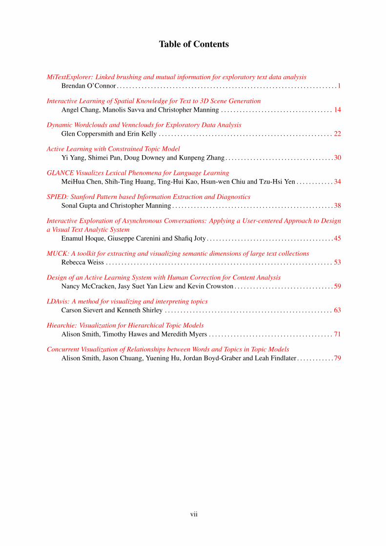
Table of Contents
MiTextExplorer: Linked brushing and mutual information for exploratory text data analysisBrendan O’Connor . . . . . . . . . . . . . . . . . . . . . . . . . . . . . . . . . . . . . . . . . . . . . . . . . . . . . . . . . . . . . . . . . . . . . . . 1
Interactive Learning of Spatial Knowledge for Text to 3D Scene GenerationAngel Chang, Manolis Savva and Christopher Manning . . . . . . . . . . . . . . . . . . . . . . . . . . . . . . . . . . . . 14
Dynamic Wordclouds and Vennclouds for Exploratory Data AnalysisGlen Coppersmith and Erin Kelly . . . . . . . . . . . . . . . . . . . . . . . . . . . . . . . . . . . . . . . . . . . . . . . . . . . . . . . . 22
Active Learning with Constrained Topic ModelYi Yang, Shimei Pan, Doug Downey and Kunpeng Zhang . . . . . . . . . . . . . . . . . . . . . . . . . . . . . . . . . . . 30
GLANCE Visualizes Lexical Phenomena for Language LearningMeiHua Chen, Shih-Ting Huang, Ting-Hui Kao, Hsun-wen Chiu and Tzu-Hsi Yen . . . . . . . . . . . . 34
SPIED: Stanford Pattern based Information Extraction and DiagnosticsSonal Gupta and Christopher Manning . . . . . . . . . . . . . . . . . . . . . . . . . . . . . . . . . . . . . . . . . . . . . . . . . . . . 38
Interactive Exploration of Asynchronous Conversations: Applying a User-centered Approach to Designa Visual Text Analytic System
Enamul Hoque, Giuseppe Carenini and Shafiq Joty . . . . . . . . . . . . . . . . . . . . . . . . . . . . . . . . . . . . . . . . . 45
MUCK: A toolkit for extracting and visualizing semantic dimensions of large text collectionsRebecca Weiss . . . . . . . . . . . . . . . . . . . . . . . . . . . . . . . . . . . . . . . . . . . . . . . . . . . . . . . . . . . . . . . . . . . . . . . . . 53
Design of an Active Learning System with Human Correction for Content AnalysisNancy McCracken, Jasy Suet Yan Liew and Kevin Crowston . . . . . . . . . . . . . . . . . . . . . . . . . . . . . . . . 59
LDAvis: A method for visualizing and interpreting topicsCarson Sievert and Kenneth Shirley . . . . . . . . . . . . . . . . . . . . . . . . . . . . . . . . . . . . . . . . . . . . . . . . . . . . . . 63
Hiearchie: Visualization for Hierarchical Topic ModelsAlison Smith, Timothy Hawes and Meredith Myers . . . . . . . . . . . . . . . . . . . . . . . . . . . . . . . . . . . . . . . . 71
Concurrent Visualization of Relationships between Words and Topics in Topic ModelsAlison Smith, Jason Chuang, Yuening Hu, Jordan Boyd-Graber and Leah Findlater . . . . . . . . . . . . 79
vii


Conference Program
Friday June 27, 2014
8:30 Opening Remarks
8:45 Invited TalkJimmy Lin
Research Papers
9:30 MiTextExplorer: Linked brushing and mutual information for exploratory text dataanalysisBrendan O’Connor
9:50 Interactive Learning of Spatial Knowledge for Text to 3D Scene GenerationAngel Chang, Manolis Savva and Christopher Manning
10:10 Dynamic Wordclouds and Vennclouds for Exploratory Data AnalysisGlen Coppersmith and Erin Kelly
10:30 Coffee Break
11:00 Invited TalkNoah Smith
11:45 Invited TalkMarti Hearst
12:30 Lunch Break
2:00 Invited TalkChris Culy
2:45 Interactive Demo Session
Active Learning with Constrained Topic ModelYi Yang, Shimei Pan, Doug Downey and Kunpeng Zhang
GLANCE Visualizes Lexical Phenomena for Language LearningMeiHua Chen, Shih-Ting Huang, Ting-Hui Kao, Hsun-wen Chiu and Tzu-Hsi Yen
SPIED: Stanford Pattern based Information Extraction and DiagnosticsSonal Gupta and Christopher Manning
Interactive Exploration of Asynchronous Conversations: Applying a User-centeredApproach to Design a Visual Text Analytic SystemEnamul Hoque, Giuseppe Carenini and Shafiq Joty
ix

Friday June 27, 2014 (continued)
Interactive Demo Session (continued)MUCK: A toolkit for extracting and visualizing semantic dimensions of large text collec-tionsRebecca Weiss
Design of an Active Learning System with Human Correction for Content AnalysisNancy McCracken, Jasy Suet Yan Liew and Kevin Crowston
LDAvis: A method for visualizing and interpreting topicsCarson Sievert and Kenneth Shirley
Hiearchie: Visualization for Hierarchical Topic ModelsAlison Smith, Timothy Hawes and Meredith Myers
Concurrent Visualization of Relationships between Words and Topics in Topic ModelsAlison Smith, Jason Chuang, Yuening Hu, Jordan Boyd-Graber and Leah Findlater
4:00 Invited TalkKrist Wongsuphasawat
4:45 Discussion and Closing Remarks
x
Proceedings of the Workshop on Interactive Language Learning, Visualization, and Interfaces, pages 1–13,Baltimore, Maryland, USA, June 27, 2014. c©2014 Association for Computational Linguistics
MITEXTEXPLORER: Linked brushing and mutual information forexploratory text data analysis
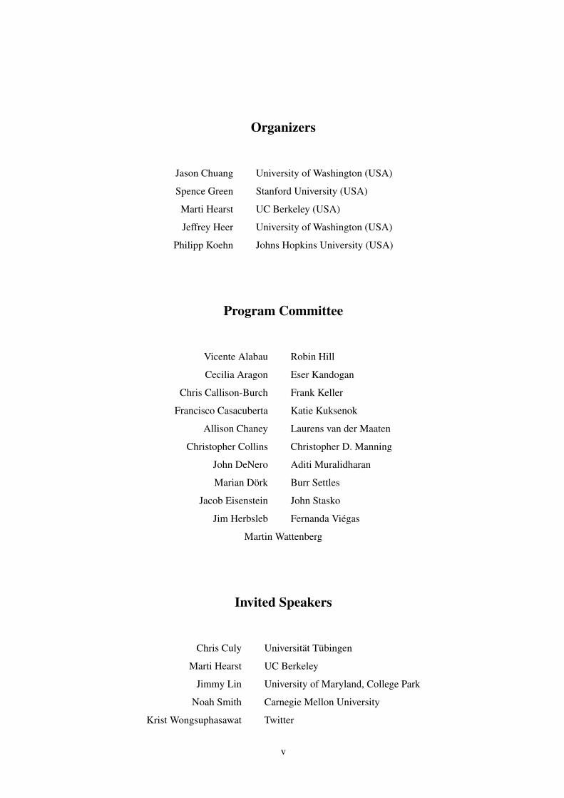
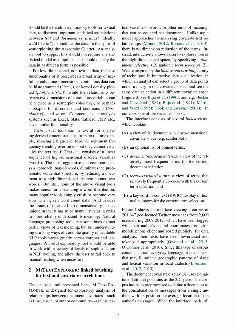
Figure 1: Screenshot of MITEXTEXPLORER, analyzing geolocated tweets.
Brendan O’ConnorMachine Learning Department
Carnegie Mellon [email protected]://brenocon.com
Abstract
In this paper I describe a preliminary ex-perimental system, MITEXTEXPLORER,for textual linked brushing, which allowsan analyst to interactively explore statis-tical relationships between (1) terms, and(2) document metadata (covariates). Ananalyst can graphically select documentsembedded in a temporal, spatial, or othercontinuous space, and the tool reportsterms with strong statistical associationsfor the region. The user can then drilldown to specific term and term groupings,viewing further associations, and see howterms are used in context. The goal is torapidly compare language usage across in-teresting document covariates.
I illustrate examples of using the tool onseveral datasets: geo-located Twitter mes-sages, presidential State of the Union ad-dresses, the ACL Anthology, and the KingJames Bible.
1 Introduction: Can we “just look” atstatistical text data?
Exploratory data analysis (EDA) is an approachto extract meaning from data, which emphasizeslearning about a dataset through an iterative pro-cess of many analyses which suggest and refinepossible hypotheses. It is vital in early stages of adata analysis for data cleaning and sanity checks,which are crucial to help ensure a dataset will beuseful. Exploratory techniques can also suggestpossible hypotheses or issues for further investi-gation.
1
3/18/14 Anscombe's_quartet_3.svg
file:///Users/brendano/projects/textexplore/writing/Anscombe's_quartet_3.svg 1/1
Figure 2: Anscombe Quartet. (Source: Wikipedia)
The classical approach to EDA, as pioneered inworks such as Tukey (1977) and Cleveland (1993)(and other work from the Bell Labs statistics groupduring that period) emphasizes visual analysis un-der nonparametric, model-free assumptions, inwhich visual attributes are a fairly direct reflec-tion of numerical or categorical aspects of data.As a simple example, consider the well-knownAnscombe Quartet (1973), a set of four bivari-ate example datasets. The Pearson correlation, avery widely used measure of dependence that as-sumes a linear Gaussian model of the data, findsthat each dataset has an identical amount of de-pendence (r = 0.82). However, a scatterplot in-stantly reveals that very different dependence re-lationships hold in each dataset (Figure 2). Thescatterplot is possibly the simplest visual analysistool for investigating the relationship between twovariables, in which the variables’ numerical valuesare mapped to horizontal and vertical space. Whilethe correlation coefficient is a model-based analy-sis tool, the scatterplot is model-free (or at least, itis effective under an arguably wider range of datagenerating assumptions), which is crucial for thisexample.
This nonparametric, visual approach to EDAhas been encoded into many data analysis pack-ages, including the now-ubiquitous R language (RCore Team, 2013), which descends from earliersoftware by the Bell Labs statistics group (Beckerand Chambers, 1984). In R, tools such as his-tograms, boxplots, barplots, dotplots, mosaicplots,etc. are built-in, basic operators in the language.(Wilkinson (2006)’s grammar of graphics moreextensively systematizes this approach; see also(Wickham, 2010; Bostock et al., 2011).)
In the meantime, textual data has emerged asa resource of increasing interest for many scien-
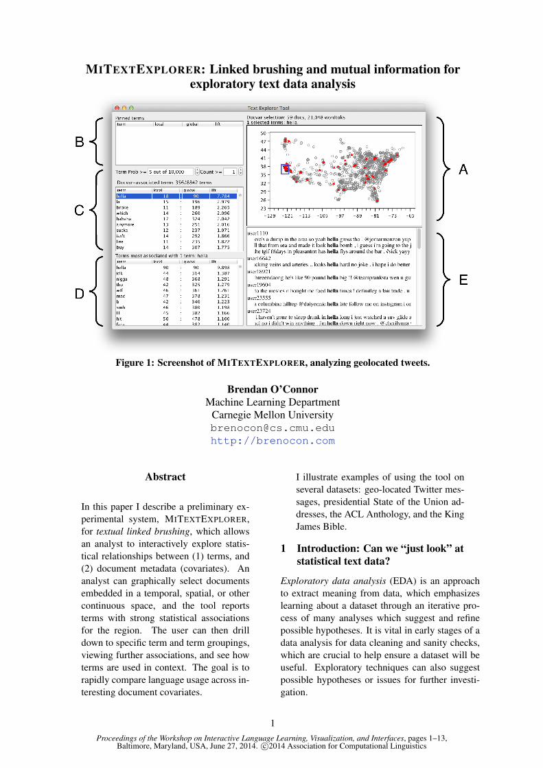
Figure 3: Linked brushing with the anal-ysis software GGobi. More references atsource: http://www.infovis-wiki.net/index.php?title=Linking_and_Brushing
tific, business, and government data analysis ap-plications. Consider the use case of automatedcontent analysis (a.k.a. text mining) as a tool forinvestigating social scientific and humanistic ques-tions (Grimmer and Stewart, 2013; Jockers, 2013;Shaw, 2012; O’Connor et al., 2011). The contentof the data is under question: analysts are inter-ested in what/when/how/by-whom different con-cepts, ideas, or attitudes are expressed in a cor-pus, and the trends in these factors across time,space, author communities, or other document-level covariates (often called metadata). Compar-isons of word statistics across covariates are ab-solutely essential to many interesting questions orsocial measurement problems, such as
• What topics tend to get censored by the Chi-nese government online, and why (Bammanet al., 2012; King et al., 2013)? Covari-ates: whether a message is deleted by cen-sors, time/location of message.
• What drives media bias? Do newspapersslant their coverage in response to what read-ers want (Gentzkow and Shapiro, 2010)? Co-variates: political preferences of readers,competitiveness of media markets.
There exist dozens, if not more, of other examplesin social scientific and humanities research; seereferences in O’Connor et al. (2011); O’Connor(2014).
In this work, I focus on the question: What
2
should be the baseline exploratory tools for textualdata, to discover important statistical associationsbetween text and document covariates? Ideally,we’d like to “just look” at the data, in the spirit ofscatterplotting the Anscombe Quartet. An analy-sis tool to support this should not require any sta-tistical model assumptions, and should display thedata in as direct a form as possible.
For low-dimensional, non-textual data, the basefunctionality of R prescribes a broad array of use-ful defaults: one-dimensional continuous data canbe histogrammed (hist(x)), or kernel density plot-ted (plot(density(x))), while the relationship be-tween two dimensions of continuous variables canbe viewed as a scatterplot (plot(x,y)); or perhapsa boxplot for discrete x and continous y (box-plot(x,y)); and so on. Commercial data analysissystems such as Excel, Stata, Tableau, JMP, etc.,have similar functionality.
These visual tools can be useful for analyz-ing derived content statistics from text—for exam-ple, showing a high-level topic or sentiment fre-quency trending over time—but they cannot visu-alize the text itself. Text data consists of a linearsequence of high-dimensional discrete variables(words). The most aggressive and common anal-ysis approach, bag-of-words, eliminates the prob-lematic sequential structure, by reducing a docu-ment to a high-dimensional discrete counts overwords. But still, none of the above visual toolsmakes sense for visualizing a word distribution;many popular tools simply crash or become veryslow when given word count data. And besidesthe issues of discrete high-dimensionality, text isunique in that it has to be manually read in orderto more reliably understand its meaning. Naturallanguage processing tools can sometimes extractpartial views of text meaning, but full understand-ing is a long ways off; and the quality of availableNLP tools varies greatly across corpora and lan-guages. A useful exploratory tool should be ableto work with a variety of levels of sophisticationin NLP tooling, and allow the user to fall back tomanual reading when necessary.
2 MITEXTEXPLORER: linked brushingfor text and covariate correlations
The analysis tool presented here, MITEXTEX-PLORER, is designed for exploratory analysis ofrelationships between document covariates—suchas time, space, or author community—against tex-
tual variables—words, or other units of meaning,that can be counted per document. Unlike topicmodel approaches to analyzing covariate-text re-lationships (Mimno, 2012; Roberts et al., 2013),there is no dimension reduction of the terms. In-stead, interactivity allows a user to explore more ofthe high-dimensional space, by specifying a doc-ument selection (Q) and/or a term selection (T ).We are inspired by the linking and brushing familyof techniques in interactive data visualization, inwhich an analyst can select a group of data pointsunder a query in one covariate space, and see thesame data selection in a different covariate space(Figure 3; see Buja et al. (1996), and e.g. Beckerand Cleveland (1987); Buja et al. (1991); Martinand Ward (1995); Cook and Swayne (2007)). Inour case, one of the variables is text.
The interface consists of several linked views,which contain:
(A) a view of the documents in a two-dimensionalcovariate space (e.g. scatterplot),
(B) an optional list of pinned terms,
(C) document-associated terms: a view of the rel-atively most frequent terms for the currentdocument selection,
(D) term-associated terms: a view of terms thatrelatively frequently co-occur with the currentterm selection; and
(E) a keyword-in-context (KWIC) display of tex-tual passages for the current term selection.
Figure 1 shows the interface viewing a corpus of201,647 geo-located Twitter messages from 2,000users during 2009-2012, which have been taggedwith their author’s spatial coordinates through amobile phone client and posted publicly; for dataanalysis, their texts have been lowercased andtokenized appropriately (Owoputi et al., 2013;O’Connor et al., 2010). Since this type of corpuscontains casual, everyday language, it is a datasetthat may illuminate geographic patterns of slangand lexical variation in local dialects (Eisensteinet al., 2012, 2010).
The document covariate display (A) uses (longi-tude, latitude) positions as the 2D space. The cor-pus has been preprocessed to define a document asthe concatenation of messages from a single au-thor, with its position the average location of theauthor’s messages. When the interface loads, all
3
points in (A) are initially gray, and all other panelsare blank.
2.1 Covariate-driven queries
A core interaction, brushing, consists of using themouse to select a rectangle in the (x,y) covariatespace. Figure 1 shows a selection around the BayArea metropolitan area (blue rectangle). Uponselection, the document-driven term display (C)is updated to show the relatively most frequentterms in the document selection. Let Q denotethe set of documents that are selected by the cur-rent covariate query. The tool ranks terms w bytheir (exponentiated) pointwise mutual informa-tion, a.k.a. lift, for Q:
lift(w; Q) =p(w|Q)p(w)
(=
p(w, Q)p(w)p(Q)
)(1)
This quantity measures how much more frequentthe term is in the queryset, compared to the base-line global probability in the corpus (p(w)). Prob-abilities are calculated with simple MLE relativefrequencies, i.e.
p(w|Q)p(w)
=
∑d∈Q ndw∑d∈Q nd
N
nw(2)
where d denotes a document ID, ndw the countof word w in document d, and N the numberof tokens in the corpus. PMI gives results thatare much more interesting than results from rank-ing w on raw probability within the query set(p(w|Q)), since that simply shows grammaticalfunction words or other terms that are commonboth in the queryset and across the corpus, and notdistinctive for the queryset.1
A well-known weakness of PMI is over-emphasis on rare terms; terms that appearonly in the queryset, even if they appear onlyonce, will attain the highest PMI value. Oneway to address this is through a smoothingprior/pseudocounts/regularization, or through sta-tistical significance ranking (see §3). For simplic-ity, we use a minimum frequency threshold filter.The user interface allows minimums for either lo-cal or global term frequencies, and to easily ad-just them, which naturally shifts the emphasis be-tween specific and generic language. All methods
1The term “lift” is used in business applications (Provostand Fawcett, 2013), while PMI has been used in many NLPapplications to measure word associations.
to protect against rare probabilistic events neces-sarily involve such a tradeoff parameter that theuser ought to experiment with; given this situation,we might prefer a transparent mechanism insteadof mathematical priors (though see also §3).
Figure 1 shows that hella is the highest rankedterm for this spatial selection (and freqency thresh-old), occurring 7.8 times more frequently com-pared to the overall corpus; this comports withsurveyed intuitions of Californian English speak-ers (Bucholtz et al., 2007). For full transparencyto the user, the local and global term counts areshown in the table. (Since hella occurred 18 timesin the queryset and 90 times globally, this im-plies the simple conditional probability p(Q|w) =18/90; and indeed, ranking on p(Q|w) is equiva-lent to ranking on PMI, since exponentiated PMIis p(Q|w)/p(Q).) The user can also sort by localcount to see the raw most-frequent term report forthe document selection. As the user reshapes thequery box, or drags it around the space, the termsin panel (C) are updated.
Not shown are options to change the term fre-quency representation. For exposition here, proba-bilities are formulated as counts of tokens, but thiscan be problematic for social media data, since asingle user might use a term a very large numberof times. The above analysis is conducted withan indicator representation of terms per user, soall frequencies refer to the probability that a useruses the term at least once. However, the other ex-amples in this paper use token-level frequencies,which seem to work fine. It is an interesting statis-tical analysis question how to derive a single rangeof methods to work across these situations.
2.2 Term selection and KWIC viewsTerms in the table (C) can be clicked and selected,forming a term selection as a set of terms T . Thisaction drives several additional views:
(A) documents containing the term are high-lighted in the document covariate display(here, in red),
(E) examples of the term’s usage, in Keyword-in-Context style with vertical alignment for thequery term; and
(D) other terms that frequently co-occur with T(§2.3).
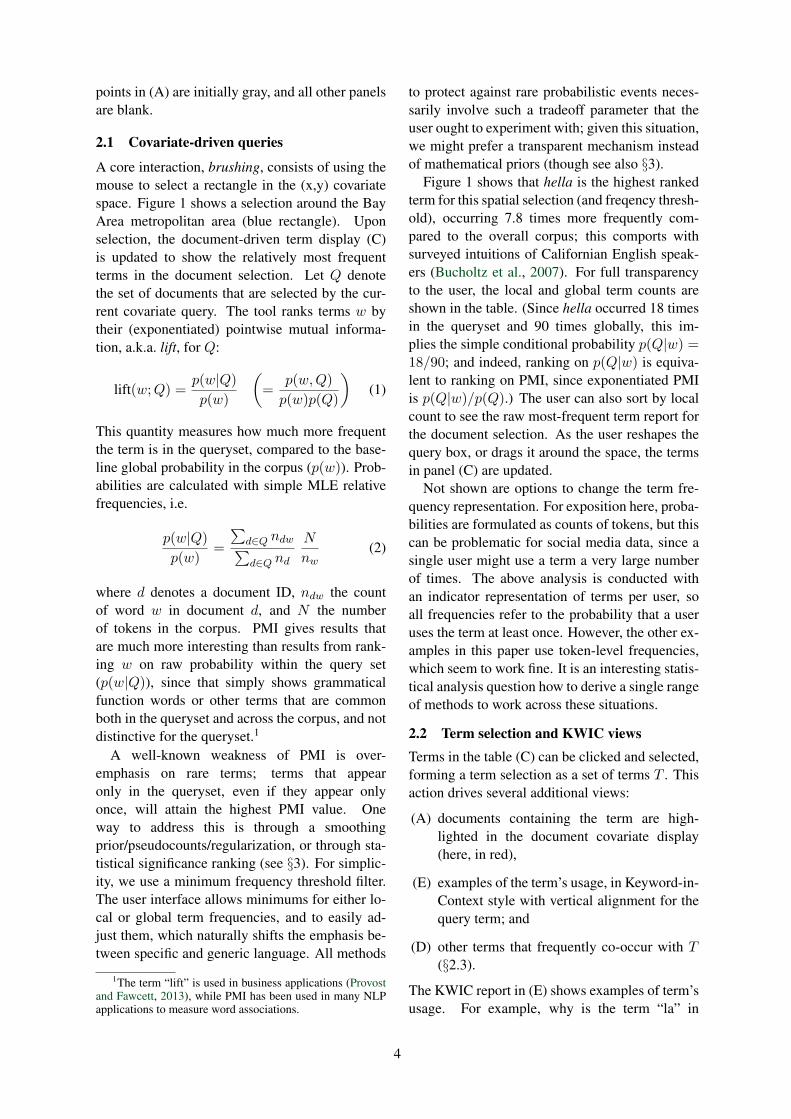
The KWIC report in (E) shows examples of term’susage. For example, why is the term “la” in
4
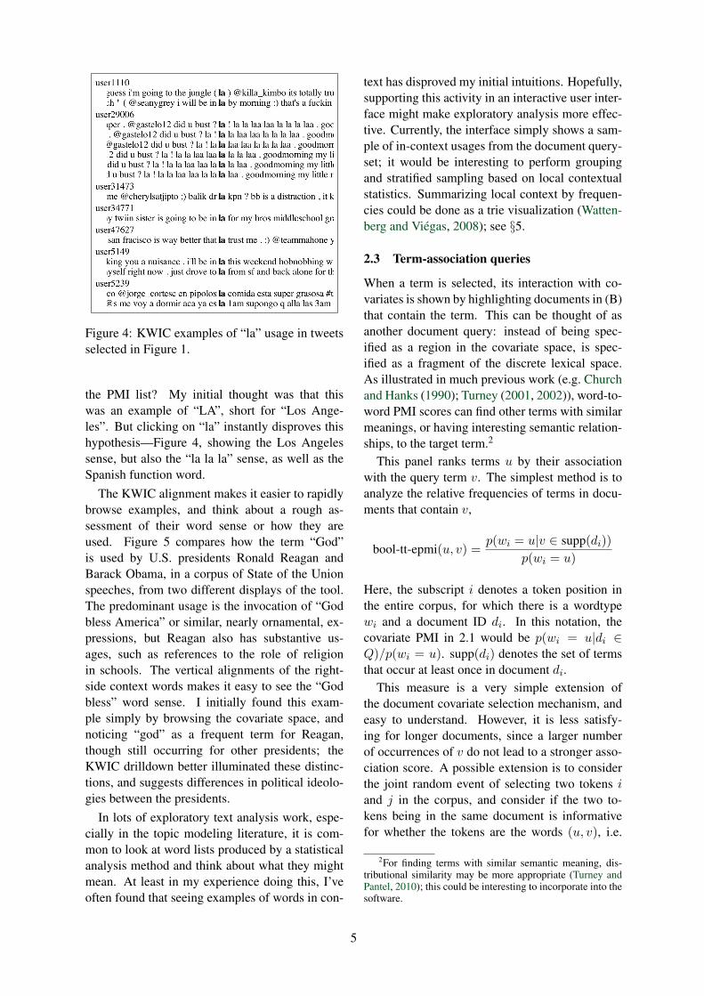
Figure 4: KWIC examples of “la” usage in tweetsselected in Figure 1.
the PMI list? My initial thought was that thiswas an example of “LA”, short for “Los Ange-les”. But clicking on “la” instantly disproves thishypothesis—Figure 4, showing the Los Angelessense, but also the “la la la” sense, as well as theSpanish function word.
The KWIC alignment makes it easier to rapidlybrowse examples, and think about a rough as-sessment of their word sense or how they areused. Figure 5 compares how the term “God”is used by U.S. presidents Ronald Reagan andBarack Obama, in a corpus of State of the Unionspeeches, from two different displays of the tool.The predominant usage is the invocation of “Godbless America” or similar, nearly ornamental, ex-pressions, but Reagan also has substantive us-ages, such as references to the role of religionin schools. The vertical alignments of the right-side context words makes it easy to see the “Godbless” word sense. I initially found this exam-ple simply by browsing the covariate space, andnoticing “god” as a frequent term for Reagan,though still occurring for other presidents; theKWIC drilldown better illuminated these distinc-tions, and suggests differences in political ideolo-gies between the presidents.
In lots of exploratory text analysis work, espe-cially in the topic modeling literature, it is com-mon to look at word lists produced by a statisticalanalysis method and think about what they mightmean. At least in my experience doing this, I’veoften found that seeing examples of words in con-
text has disproved my initial intuitions. Hopefully,supporting this activity in an interactive user inter-face might make exploratory analysis more effec-tive. Currently, the interface simply shows a sam-ple of in-context usages from the document query-set; it would be interesting to perform groupingand stratified sampling based on local contextualstatistics. Summarizing local context by frequen-cies could be done as a trie visualization (Watten-berg and Viegas, 2008); see §5.
2.3 Term-association queries
When a term is selected, its interaction with co-variates is shown by highlighting documents in (B)that contain the term. This can be thought of asanother document query: instead of being spec-ified as a region in the covariate space, is spec-ified as a fragment of the discrete lexical space.As illustrated in much previous work (e.g. Churchand Hanks (1990); Turney (2001, 2002)), word-to-word PMI scores can find other terms with similarmeanings, or having interesting semantic relation-ships, to the target term.2
This panel ranks terms u by their associationwith the query term v. The simplest method is toanalyze the relative frequencies of terms in docu-ments that contain v,
bool-tt-epmi(u, v) =p(wi = u|v ∈ supp(di))
p(wi = u)
Here, the subscript i denotes a token position inthe entire corpus, for which there is a wordtypewi and a document ID di. In this notation, thecovariate PMI in 2.1 would be p(wi = u|di ∈Q)/p(wi = u). supp(di) denotes the set of termsthat occur at least once in document di.
This measure is a very simple extension ofthe document covariate selection mechanism, andeasy to understand. However, it is less satisfy-ing for longer documents, since a larger numberof occurrences of v do not lead to a stronger asso-ciation score. A possible extension is to considerthe joint random event of selecting two tokens iand j in the corpus, and consider if the two to-kens being in the same document is informativefor whether the tokens are the words (u, v), i.e.
2For finding terms with similar semantic meaning, dis-tributional similarity may be more appropriate (Turney andPantel, 2010); this could be interesting to incorporate into thesoftware.
5
Figure 5: KWIC examples of “God” in speeches by Reagan versus Obama.
PMI[(wi, wj) = (u, v); di = dj ],
freq-tt-epmi(u, v) =p(wi = u, wj = v|di = dj)
p(wi = u, wj = v)
In terms of word counts, this expression has theform
freq-tt-epmi(u, v) =∑
d ndundv
nunv
N2∑d n2
d
The right-side term is a normalizing constant in-variant to u and v. The left-side term is interesting:it can be viewed as a similarity measure, wherethe numerator is the inner product of the invertedterm-document vectors n.,u and n.,v, and the de-nominator is the product of their `1 norms. Thisis a very similar form as cosine similarity, whichis another normalized inner product, except its de-nominator is the product of the vectors’ `2 norms.
Term-to-term associations allow a navigation ofthe term space, complementing the views of termsdriven by document covariates. This part of thetool is still at a more preliminary stage of develop-ment. One important enhancement would be ad-justment of the context window size allowed forco-occurrences; the formulations above assume acontext window the size of the document. Mediumsized context windows might capture more fo-cused topical content, especially in very long dis-courses such as speeches; and the smallest contextwindows, of size 1, should be more like colloca-tion detection (though see §3; this is arguably bet-ter done with significance tests, not PMI).
2.4 Pinned terms
The term PMI views of (C) and (D) are very dy-namic, which can cause interesting terms to disap-pear when their supporting query is changed. It isoften useful to select terms to be constantly viewedwhen the document covariate queries change.
Any term can be double-clicked to be moved tothe the table of pinned terms (B). The set of termshere does not change as the covariate query ischanged; a user can fix a set of terms and see howtheir PMI scores change while looking at differ-ent parts of the covariate space. One possible useof term pinning is to manually build up clusters ofterms—for example, topical or synonymous termsets—whose aggregate statistical behavior (i.e. asa disjunctive query) may be interesting to observe.Manually built sets of keywords are a very usefulform of text analysis; in fact, the WordSeer cor-pus analysis tool has explicit support to help userscreate them (Shrikumar, 2013).
3 Statistical term association measures
There exist many measures to measure the sta-tistical strength of an association between a termand a document covariate, or between two terms.A number of methods are based on significancetesting, looking for violations of a null hypothesisthat term frequencies are independent. For collo-cation detection, which aims to find meaningfulnon-compositional lexical items through frequen-cies of neighboring words, likelihood ratio (Dun-ning, 1993) and chi-square tests have been used(see review in Manning and Schutze (1999)). Forterm-covariate associations, chi-square tests were
6
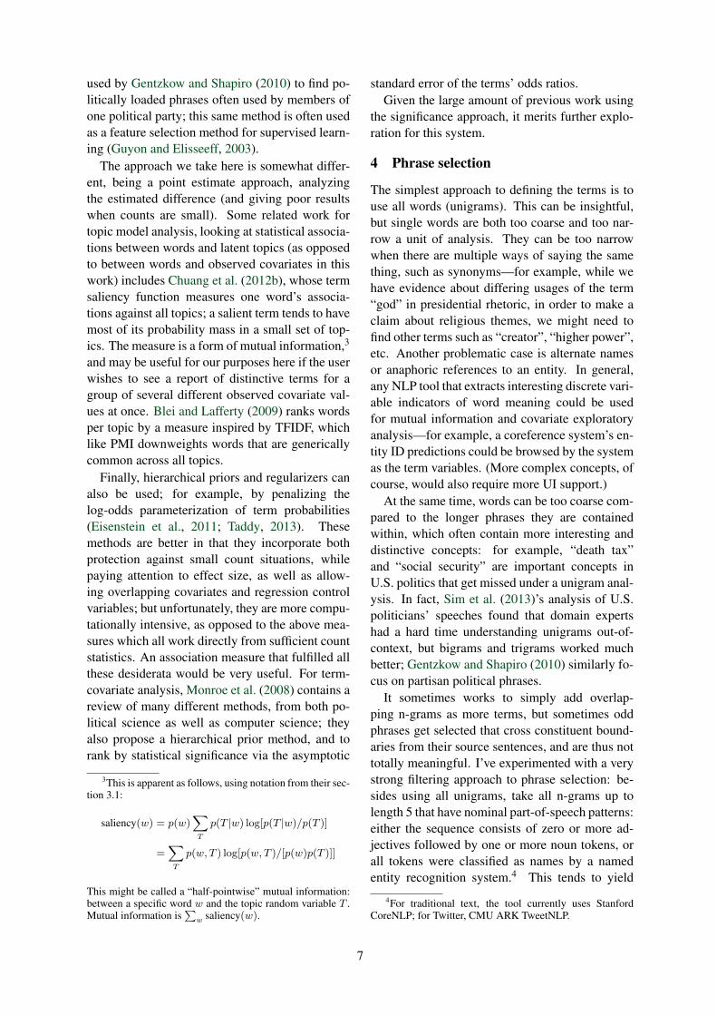
used by Gentzkow and Shapiro (2010) to find po-litically loaded phrases often used by members ofone political party; this same method is often usedas a feature selection method for supervised learn-ing (Guyon and Elisseeff, 2003).
The approach we take here is somewhat differ-ent, being a point estimate approach, analyzingthe estimated difference (and giving poor resultswhen counts are small). Some related work fortopic model analysis, looking at statistical associa-tions between words and latent topics (as opposedto between words and observed covariates in thiswork) includes Chuang et al. (2012b), whose termsaliency function measures one word’s associa-tions against all topics; a salient term tends to havemost of its probability mass in a small set of top-ics. The measure is a form of mutual information,3
and may be useful for our purposes here if the userwishes to see a report of distinctive terms for agroup of several different observed covariate val-ues at once. Blei and Lafferty (2009) ranks wordsper topic by a measure inspired by TFIDF, whichlike PMI downweights words that are genericallycommon across all topics.
Finally, hierarchical priors and regularizers canalso be used; for example, by penalizing thelog-odds parameterization of term probabilities(Eisenstein et al., 2011; Taddy, 2013). Thesemethods are better in that they incorporate bothprotection against small count situations, whilepaying attention to effect size, as well as allow-ing overlapping covariates and regression controlvariables; but unfortunately, they are more compu-tationally intensive, as opposed to the above mea-sures which all work directly from sufficient countstatistics. An association measure that fulfilled allthese desiderata would be very useful. For term-covariate analysis, Monroe et al. (2008) contains areview of many different methods, from both po-litical science as well as computer science; theyalso propose a hierarchical prior method, and torank by statistical significance via the asymptotic
3This is apparent as follows, using notation from their sec-tion 3.1:
saliency(w) = p(w)∑
T
p(T |w) log[p(T |w)/p(T )]
=∑
T
p(w, T ) log[p(w, T )/[p(w)p(T )]]
This might be called a “half-pointwise” mutual information:between a specific word w and the topic random variable T .Mutual information is
∑w saliency(w).
standard error of the terms’ odds ratios.Given the large amount of previous work using
the significance approach, it merits further explo-ration for this system.
4 Phrase selection
The simplest approach to defining the terms is touse all words (unigrams). This can be insightful,but single words are both too coarse and too nar-row a unit of analysis. They can be too narrowwhen there are multiple ways of saying the samething, such as synonyms—for example, while wehave evidence about differing usages of the term“god” in presidential rhetoric, in order to make aclaim about religious themes, we might need tofind other terms such as “creator”, “higher power”,etc. Another problematic case is alternate namesor anaphoric references to an entity. In general,any NLP tool that extracts interesting discrete vari-able indicators of word meaning could be usedfor mutual information and covariate exploratoryanalysis—for example, a coreference system’s en-tity ID predictions could be browsed by the systemas the term variables. (More complex concepts, ofcourse, would also require more UI support.)
At the same time, words can be too coarse com-pared to the longer phrases they are containedwithin, which often contain more interesting anddistinctive concepts: for example, “death tax”and “social security” are important concepts inU.S. politics that get missed under a unigram anal-ysis. In fact, Sim et al. (2013)’s analysis of U.S.politicians’ speeches found that domain expertshad a hard time understanding unigrams out-of-context, but bigrams and trigrams worked muchbetter; Gentzkow and Shapiro (2010) similarly fo-cus on partisan political phrases.
It sometimes works to simply add overlap-ping n-grams as more terms, but sometimes oddphrases get selected that cross constituent bound-aries from their source sentences, and are thus nottotally meaningful. I’ve experimented with a verystrong filtering approach to phrase selection: be-sides using all unigrams, take all n-grams up tolength 5 that have nominal part-of-speech patterns:either the sequence consists of zero or more ad-jectives followed by one or more noun tokens, orall tokens were classified as names by a namedentity recognition system.4 This tends to yield
4For traditional text, the tool currently uses StanfordCoreNLP; for Twitter, CMU ARK TweetNLP.
7
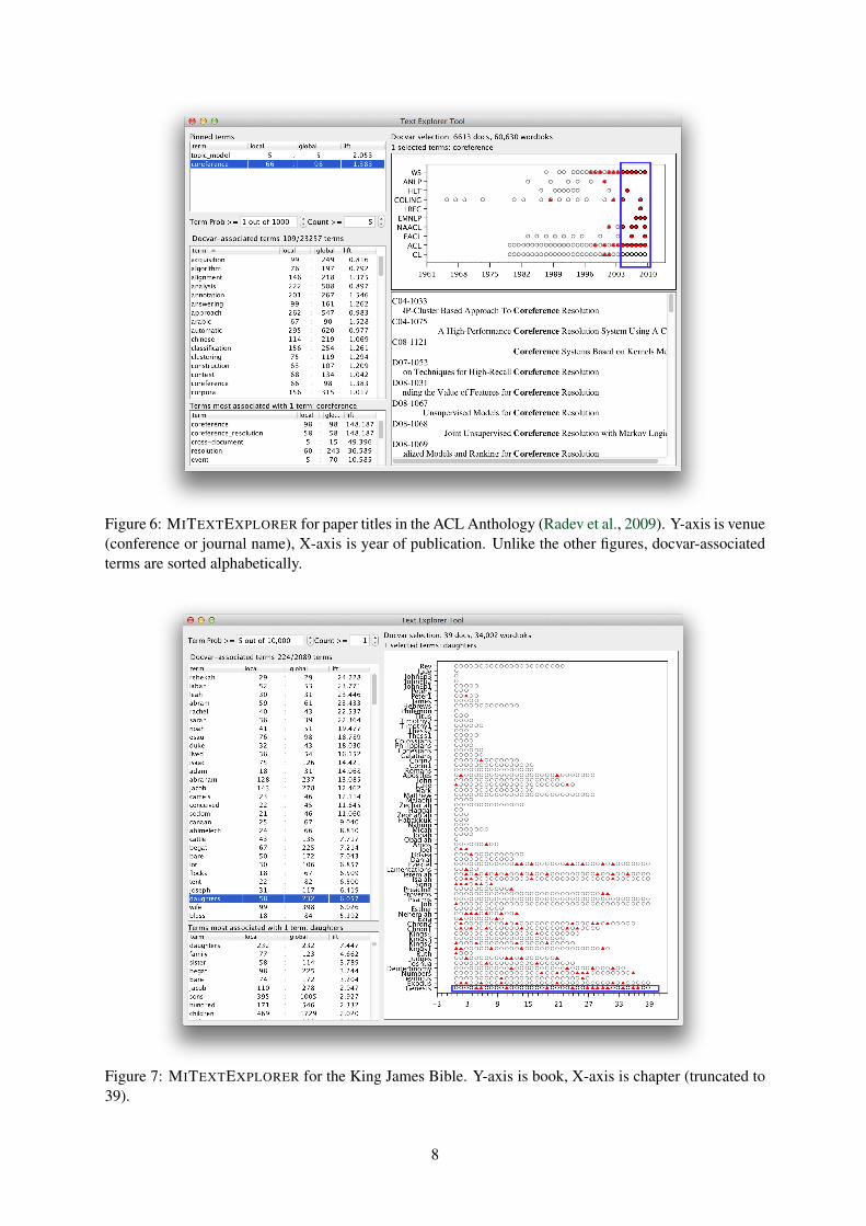
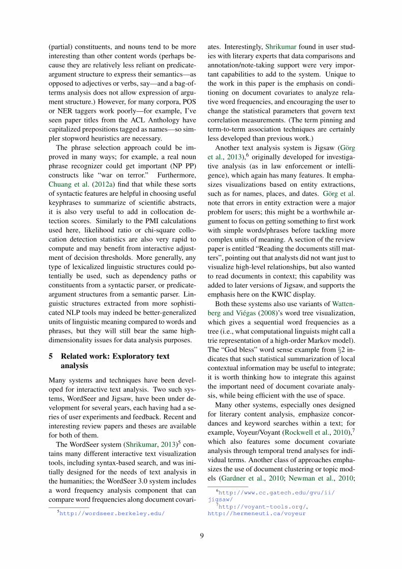
Figure 6: MITEXTEXPLORER for paper titles in the ACL Anthology (Radev et al., 2009). Y-axis is venue(conference or journal name), X-axis is year of publication. Unlike the other figures, docvar-associatedterms are sorted alphabetically.
Figure 7: MITEXTEXPLORER for the King James Bible. Y-axis is book, X-axis is chapter (truncated to39).
8
(partial) constituents, and nouns tend to be moreinteresting than other content words (perhaps be-cause they are relatively less reliant on predicate-argument structure to express their semantics—asopposed to adjectives or verbs, say—and a bag-of-terms analysis does not allow expression of argu-ment structure.) However, for many corpora, POSor NER taggers work poorly—for example, I’veseen paper titles from the ACL Anthology havecapitalized prepositions tagged as names—so sim-pler stopword heuristics are necessary.
The phrase selection approach could be im-proved in many ways; for example, a real nounphrase recognizer could get important (NP PP)constructs like “war on terror.” Furthermore,Chuang et al. (2012a) find that while these sortsof syntactic features are helpful in choosing usefulkeyphrases to summarize of scientific abstracts,it is also very useful to add in collocation de-tection scores. Similarly to the PMI calculationsused here, likelihood ratio or chi-square collo-cation detection statistics are also very rapid tocompute and may benefit from interactive adjust-ment of decision thresholds. More generally, anytype of lexicalized linguistic structures could po-tentially be used, such as dependency paths orconstituents from a syntactic parser, or predicate-argument structures from a semantic parser. Lin-guistic structures extracted from more sophisti-cated NLP tools may indeed be better-generalizedunits of linguistic meaning compared to words andphrases, but they will still bear the same high-dimensionality issues for data analysis purposes.
5 Related work: Exploratory textanalysis
Many systems and techniques have been devel-oped for interactive text analysis. Two such sys-tems, WordSeer and Jigsaw, have been under de-velopment for several years, each having had a se-ries of user experiments and feedback. Recent andinteresting review papers and theses are availablefor both of them.
The WordSeer system (Shrikumar, 2013)5 con-tains many different interactive text visualizationtools, including syntax-based search, and was ini-tially designed for the needs of text analysis inthe humanities; the WordSeer 3.0 system includesa word frequency analysis component that cancompare word frequencies along document covari-
5http://wordseer.berkeley.edu/
ates. Interestingly, Shrikumar found in user stud-ies with literary experts that data comparisons andannotation/note-taking support were very impor-tant capabilities to add to the system. Unique tothe work in this paper is the emphasis on condi-tioning on document covariates to analyze rela-tive word frequencies, and encouraging the user tochange the statistical parameters that govern textcorrelation measurements. (The term pinning andterm-to-term association techniques are certainlyless developed than previous work.)
Another text analysis system is Jigsaw (Gorget al., 2013),6 originally developed for investiga-tive analysis (as in law enforcement or intelli-gence), which again has many features. It empha-sizes visualizations based on entity extractions,such as for names, places, and dates. Gorg et al.note that errors in entity extraction were a majorproblem for users; this might be a worthwhile ar-gument to focus on getting something to first workwith simple words/phrases before tackling morecomplex units of meaning. A section of the reviewpaper is entitled “Reading the documents still mat-ters”, pointing out that analysts did not want just tovisualize high-level relationships, but also wantedto read documents in context; this capability wasadded to later versions of Jigsaw, and supports theemphasis here on the KWIC display.
Both these systems also use variants of Watten-berg and Viegas (2008)’s word tree visualization,which gives a sequential word frequencies as atree (i.e., what computational linguists might call atrie representation of a high-order Markov model).The “God bless” word sense example from §2 in-dicates that such statistical summarization of localcontextual information may be useful to integrate;it is worth thinking how to integrate this againstthe important need of document covariate analy-sis, while being efficient with the use of space.
Many other systems, especially ones designedfor literary content analysis, emphasize concor-dances and keyword searches within a text; forexample, Voyeur/Voyant (Rockwell et al., 2010),7
which also features some document covariateanalysis through temporal trend analyses for indi-vidual terms. Another class of approaches empha-sizes the use of document clustering or topic mod-els (Gardner et al., 2010; Newman et al., 2010;
6http://www.cc.gatech.edu/gvu/ii/jigsaw/
7http://voyant-tools.org/,http://hermeneuti.ca/voyeur
9
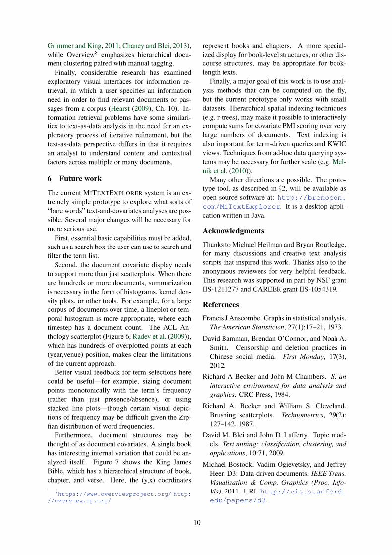
Grimmer and King, 2011; Chaney and Blei, 2013),while Overview8 emphasizes hierarchical docu-ment clustering paired with manual tagging.
Finally, considerable research has examinedexploratory visual interfaces for information re-trieval, in which a user specifies an informationneed in order to find relevant documents or pas-sages from a corpus (Hearst (2009), Ch. 10). In-formation retrieval problems have some similari-ties to text-as-data analysis in the need for an ex-ploratory process of iterative refinement, but thetext-as-data perspective differs in that it requiresan analyst to understand content and contextualfactors across multiple or many documents.
6 Future work
The current MITEXTEXPLORER system is an ex-tremely simple prototype to explore what sorts of“bare words” text-and-covariates analyses are pos-sible. Several major changes will be necessary formore serious use.
First, essential basic capabilities must be added,such as a search box the user can use to search andfilter the term list.
Second, the document covariate display needsto support more than just scatterplots. When thereare hundreds or more documents, summarizationis necessary in the form of histograms, kernel den-sity plots, or other tools. For example, for a largecorpus of documents over time, a lineplot or tem-poral histogram is more appropriate, where eachtimestep has a document count. The ACL An-thology scatterplot (Figure 6, Radev et al. (2009)),which has hundreds of overplotted points at each(year,venue) position, makes clear the limitationsof the current approach.
Better visual feedback for term selections herecould be useful—for example, sizing documentpoints monotonically with the term’s frequency(rather than just presence/absence), or usingstacked line plots—though certain visual depic-tions of frequency may be difficult given the Zip-fian distribution of word frequencies.
Furthermore, document structures may bethought of as document covariates. A single bookhas interesting internal variation that could be an-alyzed itself. Figure 7 shows the King JamesBible, which has a hierarchical structure of book,chapter, and verse. Here, the (y,x) coordinates
8https://www.overviewproject.org/ http://overview.ap.org/
represent books and chapters. A more special-ized display for book-level structures, or other dis-course structures, may be appropriate for book-length texts.
Finally, a major goal of this work is to use anal-ysis methods that can be computed on the fly,but the current prototype only works with smalldatasets. Hierarchical spatial indexing techniques(e.g. r-trees), may make it possible to interactivelycompute sums for covariate PMI scoring over verylarge numbers of documents. Text indexing isalso important for term-driven queries and KWICviews. Techniques from ad-hoc data querying sys-tems may be necessary for further scale (e.g. Mel-nik et al. (2010)).
Many other directions are possible. The proto-type tool, as described in §2, will be available asopen-source software at: http://brenocon.com/MiTextExplorer. It is a desktop appli-cation written in Java.
Acknowledgments
Thanks to Michael Heilman and Bryan Routledge,for many discussions and creative text analysisscripts that inspired this work. Thanks also to theanonymous reviewers for very helpful feedback.This research was supported in part by NSF grantIIS-1211277 and CAREER grant IIS-1054319.
References
Francis J Anscombe. Graphs in statistical analysis.The American Statistician, 27(1):17–21, 1973.
David Bamman, Brendan O’Connor, and Noah A.Smith. Censorship and deletion practices inChinese social media. First Monday, 17(3),2012.
Richard A Becker and John M Chambers. S: aninteractive environment for data analysis andgraphics. CRC Press, 1984.
Richard A. Becker and William S. Cleveland.Brushing scatterplots. Technometrics, 29(2):127–142, 1987.
David M. Blei and John D. Lafferty. Topic mod-els. Text mining: classification, clustering, andapplications, 10:71, 2009.
Michael Bostock, Vadim Ogievetsky, and JeffreyHeer. D3: Data-driven documents. IEEE Trans.Visualization & Comp. Graphics (Proc. Info-Vis), 2011. URL http://vis.stanford.edu/papers/d3.
10
Mary Bucholtz, Nancy Bermudez, Victor Fung,Lisa Edwards, and Rosalva Vargas. HellaNor Cal or totally So Cal? the per-ceptual dialectology of California. Jour-nal of English Linguistics, 35(4):325–352,2007. URL http://people.duke.edu/
˜eec10/hellanorcal.pdf.
Andreas Buja, John Alan McDonald, John Micha-lak, and Werner Stuetzle. Interactive data visu-alization using focusing and linking. In Visu-alization, 1991. Visualization’91, Proceedings.,IEEE Conference on, pages 156–163. IEEE,1991.
Andreas Buja, Dianne Cook, and Deborah FSwayne. Interactive high-dimensional data vi-sualization. Journal of Computational andGraphical Statistics, 5(1):78–99, 1996.
Allison J.B. Chaney and David M. Blei. Visual-izing topic models. In Proceedings of ICWSM,2013.
Jason Chuang, Christopher D. Manning, andJeffrey Heer. ”without the clutter of unim-portant words”: Descriptive keyphrases fortext visualization. ACM Trans. on Computer-Human Interaction, 19:1–29, 2012a. URLhttp://vis.stanford.edu/papers/keyphrases.
Jason Chuang, Christopher D. Manning, and Jef-frey Heer. Termite: Visualization techniques forassessing textual topic models. In Advanced Vi-sual Interfaces, 2012b. URL http://vis.stanford.edu/papers/termite.
K. W Church and P. Hanks. Word associationnorms, mutual information, and lexicography.Computational linguistics, 16(1):2229, 1990.
William S. Cleveland. Visualizing data. HobartPress, 1993.
Dianne Cook and Deborah F. Swayne. Interactiveand dynamic graphics for data analysis: with Rand GGobi. Springer, 2007.
Ted Dunning. Accurate methods for the statisticsof surprise and coincidence. Computa-tional Linguistics, 19:61—74, 1993. doi:10.1.1.14.5962. URL http://citeseerx.ist.psu.edu/viewdoc/summary?doi=10.1.1.14.5962.
J. Eisenstein, A. Ahmed, and E.P. Xing. Sparse ad-ditive generative models of text. In Proceedingsof ICML, pages 1041–1048, 2011.
Jacob Eisenstein, Brendan O’Connor, Noah A.Smith, and Eric P. Xing. A latent variable modelfor geographic lexical variation. In Proceedingsof the 2010 Conference on Empirical Methodsin Natural Language Processing, pages 1277—1287, 2010.
Jacob Eisenstein, Brendan O’Connor, Noah A.Smith, and Eric P. Xing. Mapping the geograph-ical diffusion of new words. In NIPS Workshopon Social Network and Social Media Analy-sis, 2012. URL http://arxiv.org/abs/1210.5268.
M.J. Gardner, J. Lutes, J. Lund, J. Hansen,D. Walker, E. Ringger, and K. Seppi. The topicbrowser: An interactive tool for browsing topicmodels. In NIPS Workshop on Challenges ofData Visualization. MIT Press, 2010.
Matthew Gentzkow and Jesse M Shapiro. Whatdrives media slant? evidence from us dailynewspapers. Econometrica, 78(1):35–71, 2010.
Carsten Gorg, Zhicheng Liu, and John Stasko.Reflections on the evolution of the jigsaw vi-sual analytics system. Information Visualiza-tion, 2013.
Justin Grimmer and Gary King. General purposecomputer-assisted clustering and conceptualiza-tion. Proceedings of the National Academy ofSciences, 108(7):2643–2650, 2011.
Justin Grimmer and Brandon M Stewart. Textas Data: The promise and pitfalls of au-tomatic content analysis methods for polit-ical texts. Political Analysis, 21(3):267–297, 2013. URL http://www.stanford.edu/˜jgrimmer/tad2.pdf.
Isabelle Guyon and Andre Elisseeff. An introduc-tion to variable and feature selection. The Jour-nal of Machine Learning Research, 3:1157–1182, 2003.
Marti Hearst. Search user interfaces. CambridgeUniversity Press, 2009.
Matthew L Jockers. Macroanalysis: Digital meth-ods and literary history. University of IllinoisPress, 2013.
Gary King, Jennifer Pan, and Margaret E. Roberts.How censorship in china allows governmentcriticism but silences collective expression.American Political Science Review, 107:1–18,2013.
11
Christopher D Manning and Hinrich Schutze.Foundations of statistical natural language pro-cessing. MIT press, 1999.
Allen R. Martin and Matthew O. Ward. High di-mensional brushing for interactive explorationof multivariate data. In Proceedings of the6th Conference on Visualization’95, page 271.IEEE Computer Society, 1995.
Sergey Melnik, Andrey Gubarev, Jing Jing Long,Geoffrey Romer, Shiva Shivakumar, MattTolton, and Theo Vassilakis. Dremel: interac-tive analysis of web-scale datasets. Proceed-ings of the VLDB Endowment, 3(1-2):330–339,2010.
David Mimno. Topic regression. PhD thesis, Uni-versity of Massachusetts Amherst, 2012.
B. L. Monroe, M. P. Colaresi, and K. M. Quinn.Fightin’Words: lexical feature selection andevaluation for identifying the content of politi-cal conflict. Political Analysis, 16(4):372, 2008.
D. Newman, T. Baldwin, L. Cavedon, E. Huang,S. Karimi, D. Martinez, F. Scholer, and J. Zo-bel. Visualizing search results and documentcollections using topic maps. Web Semantics:Science, Services and Agents on the World WideWeb, 8(2):169–175, 2010.
Brendan O’Connor. Statistical Text Analysis forSocial Science. PhD thesis, Carnegie MellonUniversity, 2014.
Brendan O’Connor, Michel Krieger, and DavidAhn. TweetMotif: Exploratory search and topicsummarization for Twitter. In Proceedings ofthe International AAAI Conference on Weblogsand Social Media, 2010.
Brendan O’Connor, David Bamman, and Noah A.Smith. Computational text analysis for socialscience: Model assumptions and complexity. InSecond Workshop on Comptuational Social Sci-ence and the Wisdom of Crowds (NIPS 2011),2011.
Olutobi Owoputi, Brendan O’Connor, Chris Dyer,Kevin Gimpel, Nathan Schneider, and Noah ASmith. Improved part-of-speech tagging for on-line conversational text with word clusters. InProceedings of NAACL, 2013.
Foster Provost and Tom Fawcett. Data Science forBusiness. O’Reilly Media, 2013.
R Core Team. R: A Language and Environment forStatistical Computing. R Foundation for Statis-
tical Computing, Vienna, Austria, 2013. URLhttp://www.R-project.org/. ISBN 3-900051-07-0.
Dragomir R. Radev, Pradeep Muthukrishnan, andVahed Qazvinian. The ACL anthology networkcorpus. In Proc. of ACL Workshop on Natu-ral Language Processing and Information Re-trieval for Digital Libraries, 2009.
Margaret E. Roberts, Brandon M. Stewart, andEdoardo M. Airoldi. Structural topic models.2013. URL http://scholar.harvard.edu/bstewart/publications/structural-topic-models. Work-ing paper.
Geoffrey Rockwell, Stefan G Sinclair, StanRuecker, and Peter Organisciak. Ubiquitoustext analysis. paj: The Journal of the Initiativefor Digital Humanities, Media, and Culture, 2(1), 2010.
Ryan Shaw. Text-mining as a researchtool, 2012. URL http://aeshin.org/textmining/.
Aditi Shrikumar. Designing an Exploratory TextAnalysis Tool for Humanities and Social Sci-ences Research. PhD thesis, University of Cali-fornia at Berkeley, 2013.
Yanchuan Sim, Brice Acree, Justin H Gross, andNoah A Smith. Measuring ideological propor-tions in political speeches. In Proceedings ofEMNLP, 2013.
Matt Taddy. Multinomial inverse regression fortext analysis. Journal of the American Statisti-cal Association, 108(503):755–770, 2013.
John W. Tukey. Exploratory data analysis. 1977.
P. D Turney. Thumbs up or thumbs down?: seman-tic orientation applied to unsupervised classifi-cation of reviews. In Proceedings of the 40thAnnual Meeting on Association for Computa-tional Linguistics, page 417424, 2002.
P. D Turney and P. Pantel. From frequency tomeaning: Vector space models of semantics.Journal of Artificial Intelligence Research, 37(1):141188, 2010. ISSN 1076-9757.
Peter Turney. Mining the web for syn-onyms: Pmi-ir versus lsa on toefl. InProceedings of the Twelth European Con-ference on Machine Learning, 2001.URL http://nparc.cisti-icist.
12

nrc-cnrc.gc.ca/npsi/ctrl?action=rtdoc&an=5765594.
Martin Wattenberg and Fernanda B Viegas. Theword tree, an interactive visual concordance.Visualization and Computer Graphics, IEEETransactions on, 14(6):1221–1228, 2008.
Hadley Wickham. A layered grammar of graph-ics. Journal of Computational and GraphicalStatistics, 19(1):328, 2010. doi: 10.1198/jcgs.2009.07098.
Leland Wilkinson. The grammar of graphics.Springer, 2006.
13
Proceedings of the Workshop on Interactive Language Learning, Visualization, and Interfaces, pages 14–21,Baltimore, Maryland, USA, June 27, 2014. c©2014 Association for Computational Linguistics
Interactive Learning of Spatial Knowledgefor Text to 3D Scene Generation
Angel X. Chang, Manolis Savva and Christopher D. ManningComputer Science Department, Stanford University{angelx,msavva,manning}@cs.stanford.edu
Abstract
We present an interactive text to 3D scenegeneration system that learns the expectedspatial layout of objects from data. A userprovides input natural language text fromwhich we extract explicit constraints onthe objects that should appear in the scene.Given these explicit constraints, the sys-tem then uses prior observations of spa-tial arrangements in a database of scenesto infer the most likely layout of the ob-jects in the scene. Through further userinteraction, the system gradually adjustsand improves its estimates of where ob-jects should be placed. We present exam-ple generated scenes and user interactionscenarios.
1 Introduction
People possess the power of visual imaginationthat allows them to turn descriptions of scenes intoimagery. The conceptual simplicity of generatingpictures from descriptions has spurred the desireto make systems capable of this task. However, re-search into computational systems for creating im-agery from textual descriptions has seen only lim-ited success.Most current 3D scene design systems require
the user to learn complex manipulation interfacesthrough which objects are constructed and pre-cisely positioned within scenes. However, arrang-ing objects in scenes can much more easily beachieved using natural language. For instance, itis much easier to say “Put a cup on the table’,rather than having to search for a 3D model of acup, insert it into the scene, scale it to the correctsize, orient it, and position it on a table ensuringit maintains contact with the table. By making3D scene design more accessible to novice userswe empower a broader demographic to create 3D
scenes for use cases such as interior design, virtualstoryboarding and personalized augmented reality.Unfortunately, several key technical challenges
restrict our ability to create text to 3D scene sys-tems. Natural language is difficult to map to for-mal representations of spatial knowledge and con-straints. Furthermore, language rarely mentionscommon sense facts about the world, that containcritically important spatial knowledge. For exam-ple, people do not usually mention the presence ofthe ground or that most objects are supported by it.As a consequence, spatial knowledge is severelylacking in current computational systems.Pioneering work in mapping text to 3D scene
representations has taken two approaches to ad-dress these challenges. First, by restricting the dis-course domain to a micro-world with simple geo-metric shapes, the SHRDLU system demonstratedparsing of natural language input for manipulatingthe scene, and learning of procedural knowledgethrough interaction (Winograd, 1972). However,generalization to scenes with more complex ob-jects and spatial relations is very hard to attain.More recently, the WordsEye system has fo-
cused on the general text to 3D scene generationtask (Coyne and Sproat, 2001), allowing a userto generate a 3D scene directly from a textual de-scription of the objects present, their properties andtheir spatial arrangement. The authors of Words-Eye demonstrated the promise of text to scene gen-eration systems but also pointed out some funda-mental issues which restrict the success of theirsystem: a lot of spatial knowledge is requiredwhich is hard to obtain. As a result, the user has touse unnatural language (e.g. “the stool is 1 feet tothe south of the table”) to express their intent.For a text to scene system to understand more
natural text, it must be able to infer implicit in-formation not explicitly stated in the text. For in-stance, given the sentence “there is an office witha red chair”, the system should be able to infer
14
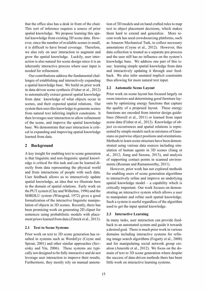
that the office also has a desk in front of the chair.This sort of inference requires a source of priorspatial knowledge. We propose learning this spa-tial knowledge from existing 3D scene data. How-ever, since the number of available scenes is small,it is difficult to have broad coverage. Therefore,we also rely on user interaction to augment andgrow the spatial knowledge. Luckily, user inter-action is also natural for scene design since it is aninherently interactive process where user input isneeded for refinement.Our contributions address the fundamental chal-
lenges of establishing and interactively expandinga spatial knowledge base. We build on prior workin data-driven scene synthesis (Fisher et al., 2012)to automatically extract general spatial knowledgefrom data: knowledge of what objects occur inscenes, and their expected spatial relations. Oursystem then uses this knowledge to generate scenesfrom natural text inferring implicit constraints. Itthen leverages user interaction to allow refinementof the scene, and improve the spatial knowledgebase. We demonstrate that user interaction is criti-cal in expanding and improving spatial knowledgelearned from data.
2 Background
A key insight for enabling text to scene generationis that linguistic and non-linguistic spatial knowl-edge is critical for this task and can be learned di-rectly from data representing the physical worldand from interactions of people with such data.User feedback allows us to interactively updatespatial knowledge, an idea that we illustrate herein the domain of spatial relations. Early work onthe PUT system (Clay andWilhelms, 1996) and theSHRDLU system (Winograd, 1972) gives a goodformalization of the interactive linguistic manipu-lation of objects in 3D scenes. Recently, there hasbeen promising work on generating 2D clipart forsentences using probabilistic models with place-ment priors learned from data (Zitnick et al., 2013).
2.1 Text to Scene Systems
Prior work on text to 3D scene generation has re-sulted in systems such as WordsEye (Coyne andSproat, 2001) and other similar approaches (Sev-ersky and Yin, 2006). These systems are typi-cally not designed to be fully interactive and do notleverage user interaction to improve their results.Furthermore, they mostly rely on manual annota-
tion of 3Dmodels and on hand crafted rules to maptext to object placement decisions, which makesthem hard to extend and generalize. More re-cent work has used crowdsourcing platforms, suchas Amazon Mechanical Turk, to collect necessaryannotations (Coyne et al., 2012). However, thisdata collection is treated as a separate pre-processand the user still has no influence on the system’sknowledge base. We address one part of this is-sue: learning simple spatial knowledge from dataand interactively updating it through user feed-back. We also infer unstated implicit constraintsthus allowing for more natural text input.
2.2 Automatic Scene LayoutPrior work on scene layout has focused largely onroom interiors and determining good furniture lay-outs by optimizing energy functions that capturethe quality of a proposed layout. These energyfunctions are encoded from interior design guide-lines (Merrell et al., 2011) or learned from inputscene data (Fisher et al., 2012). Knowledge of ob-ject co-occurrences and spatial relations is repre-sented by simple models such as mixtures of Gaus-sians on pairwise object positions and orientations.Methods to learn scene structure have been demon-strated using various data sources including sim-ulation of human agents in 3D scenes (Jiang etal., 2012; Jiang and Saxena, 2013), and analysisof supporting contact points in scanned environ-ments (Rosman and Ramamoorthy, 2011).However, prior work has not explored methods
for enabling users of scene generation algorithmsto interactively refine and improve an underlyingspatial knowledge model – a capability which iscritically important. Our work focuses on demon-strating an interactive system which allows a userto manipulate and refine such spatial knowledge.Such a system is useful regardless of the algorithmused to get the input spatial knowledge.
2.3 Interactive LearningIn many tasks, user interaction can provide feed-back to an automated system and guide it towardsa desired goal. There is much prior work in variousdomains including interactive systems for refin-ing image search algorithms (Fogarty et al., 2008)and for manipulating social network group cre-ation (Amershi et al., 2012). We focus on the do-main of text to 3D scene generation where despitethe success of data-driven methods there has beenlittle work on interactive learning systems.
15
3 Approach Overview
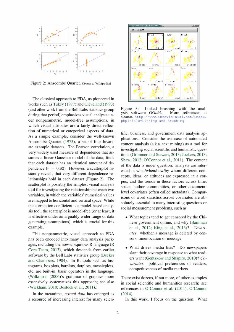
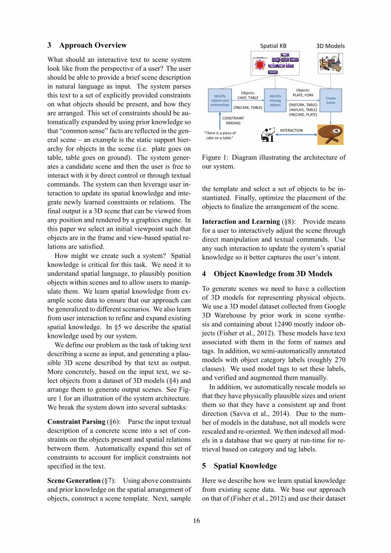
What should an interactive text to scene systemlook like from the perspective of a user? The usershould be able to provide a brief scene descriptionin natural language as input. The system parsesthis text to a set of explicitly provided constraintson what objects should be present, and how theyare arranged. This set of constraints should be au-tomatically expanded by using prior knowledge sothat “common sense” facts are reflected in the gen-eral scene – an example is the static support hier-archy for objects in the scene (i.e. plate goes ontable, table goes on ground). The system gener-ates a candidate scene and then the user is free tointeract with it by direct control or through textualcommands. The system can then leverage user in-teraction to update its spatial knowledge and inte-grate newly learned constraints or relations. Thefinal output is a 3D scene that can be viewed fromany position and rendered by a graphics engine. Inthis paper we select an initial viewpoint such thatobjects are in the frame and view-based spatial re-lations are satisfied.How might we create such a system? Spatial
knowledge is critical for this task. We need it tounderstand spatial language, to plausibly positionobjects within scenes and to allow users to manip-ulate them. We learn spatial knowledge from ex-ample scene data to ensure that our approach canbe generalized to different scenarios. We also learnfrom user interaction to refine and expand existingspatial knowledge. In §5 we describe the spatialknowledge used by our system.We define our problem as the task of taking text
describing a scene as input, and generating a plau-sible 3D scene described by that text as output.More concretely, based on the input text, we se-lect objects from a dataset of 3D models (§4) andarrange them to generate output scenes. See Fig-ure 1 for an illustration of the system architecture.We break the system down into several subtasks:
Constraint Parsing (§6): Parse the input textualdescription of a concrete scene into a set of con-straints on the objects present and spatial relationsbetween them. Automatically expand this set ofconstraints to account for implicit constraints notspecified in the text.
SceneGeneration (§7): Using above constraintsand prior knowledge on the spatial arrangement ofobjects, construct a scene template. Next, sample
Objects:
PLATE, FORK
ON(FORK, TABLE)
ON(PLATE, TABLE)
ON(CAKE, PLATE)
“There is a piece of
cake on a table.”
Create
Scene
Identify
missing
objects
3D ModelsSpatial KB
Objects:
CAKE, TABLE
ON(CAKE, TABLE)
Identify
objects and
relationships
INTERACTION
CONSTRAINT
PARSING
Figure 1: Diagram illustrating the architecture ofour system.
the template and select a set of objects to be in-stantiated. Finally, optimize the placement of theobjects to finalize the arrangement of the scene.
Interaction and Learning (§8): Provide meansfor a user to interactively adjust the scene throughdirect manipulation and textual commands. Useany such interaction to update the system’s spatialknowledge so it better captures the user’s intent.
4 Object Knowledge from 3D Models
To generate scenes we need to have a collectionof 3D models for representing physical objects.We use a 3D model dataset collected from Google3D Warehouse by prior work in scene synthe-sis and containing about 12490 mostly indoor ob-jects (Fisher et al., 2012). These models have textassociated with them in the form of names andtags. In addition, we semi-automatically annotatedmodels with object category labels (roughly 270classes). We used model tags to set these labels,and verified and augmented them manually.In addition, we automatically rescale models so
that they have physically plausible sizes and orientthem so that they have a consistent up and frontdirection (Savva et al., 2014). Due to the num-ber of models in the database, not all models wererescaled and re-oriented. We then indexed all mod-els in a database that we query at run-time for re-trieval based on category and tag labels.
5 Spatial Knowledge
Here we describe how we learn spatial knowledgefrom existing scene data. We base our approachon that of (Fisher et al., 2012) and use their dataset
16
of 133 small indoor scenes created with 1723 3DWarehouse models. Relative object-to-object po-sition and orientation priors can also be learnedfrom the scene data but we have not yet incorpo-rated them in the results for this paper.
5.1 Support HierarchyWe observe the static support relations of objectsin existing scenes to establish a prior over what ob-jects go on top of what other objects. As an exam-ple, by observing plates and forks on tables mostof the time, we establish that tables are more likelyto support plates and forks than chairs. We esti-mate the probability of a parent category Cp sup-porting a given child category Cc as a simple con-ditional probability based on normalized observa-tion counts.
Psupport(Cp|Cc) =count(Cc on Cp)
count(Cc)
5.2 Supporting surfacesTo identify which surfaces on parent objects sup-port child objects, we first segment parent modelsinto planar surfaces using a simple region-growingalgorithm based on (Kalvin and Taylor, 1996). Wecharacterize support surfaces by the direction oftheir normal vector limited to the six canonical di-rections: up, down, left, right, front, back. We thenlearn a probability of supporting surface normaldirection Sn given child object category Cc. Forexample, posters are typically found on walls sotheir support normal vectors are in the horizontaldirections. Any unobserved child categories areassumed to have Psurf (Sn = up|Cc) = 1 sincemost things rest on a horizontal surface (e.g. floor).
Psurf (Sn|Cc) =count(Cc on surface with Sn)
count(Cc)
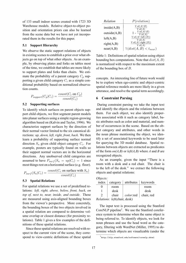
5.3 Spatial RelationsFor spatial relations we use a set of predefined re-lations: left, right, above, below, front, back, ontop of, next to, near, inside, and outside. Theseare measured using axis-aligned bounding boxesfrom the viewer’s perspective. More concretely,the bounding boxes of the two objects involved ina spatial relation are compared to determine vol-ume overlap or closest distance (for proximity re-lations). Table 1 gives a few examples of the defi-nitions of these spatial relations.Since these spatial relations are resolvedwith re-
spect to the current view of the scene, they corre-spond to view-centric definitions of these spatial
Relation P (relation)
inside(A,B) V ol(A∩B)V ol(A)
outside(A,B) 1 - V ol(A∩B)V ol(A)
left(A,B) V ol(A∩ left (B))V ol(A)
right(A,B) V ol(A∩ right (B))V ol(A)
near(A,B) 1(dist(A,B) < tnear)
Table 1: Definitions of spatial relation using objectbounding box computations. Note that dist(A,B)is normalized with respect to the maximum extentof the bounding box of B.
concepts. An interesting line of future work wouldbe to explore when ego-centric and object-centricspatial reference models are more likely in a givenutterance, and resolve the spatial term accordingly.
6 Constraint Parsing
During constraint parsing we take the input textand identify the objects and the relations betweenthem. For each object, we also identify proper-ties associated with it such as category label, ba-sic attributes such as color and material, and num-ber of occurrences in the scene. Based on the ob-ject category and attributes, and other words inthe noun phrase mentioning the object, we iden-tify a set of associated keywords to be used laterfor querying the 3D model database. Spatial re-lations between objects are extracted as predicatesof the form on(A,B) or left(A,B) where A and B arerecognized objects.As an example, given the input “There is a
room with a desk and a red chair. The chair isto the left of the desk.” we extract the followingobjects and spatial relations:
Objects:index category attributes keywords0 room room1 desk desk2 chair color:red chair, red
Relations: left(chair, desk)
The input text is processed using the StanfordCoreNLP pipeline1. We use the Stanford corefer-ence system to determine when the same object isbeing referred to. To identify objects, we look fornoun phrases and use the head word as the cate-gory, filtering with WordNet (Miller, 1995) to de-termine which objects are visualizable (under the
1http://nlp.stanford.edu/software/corenlp.shtml
17
Dependency Pattern Example Text
tag:VBN=verb >nsubjpass =nsubj >prep (=prep >pobj =pobj) The chair[nsubj] is made[verb] of[prep] wood[pobj]
tag:VB=verb >dobj =dobj >prep (=prep >pobj =pobj) Put[verb] the cup[dobj] on[prep] the table[pobj]
Table 2: Example dependency patterns for extracting spatial relations.
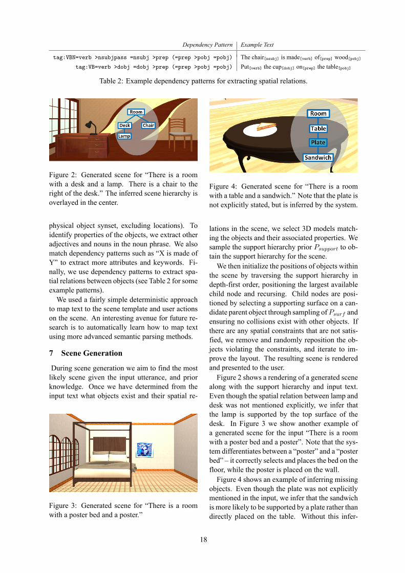
Figure 2: Generated scene for “There is a roomwith a desk and a lamp. There is a chair to theright of the desk.” The inferred scene hierarchy isoverlayed in the center.
physical object synset, excluding locations). Toidentify properties of the objects, we extract otheradjectives and nouns in the noun phrase. We alsomatch dependency patterns such as “X is made ofY” to extract more attributes and keywords. Fi-nally, we use dependency patterns to extract spa-tial relations between objects (see Table 2 for someexample patterns).We used a fairly simple deterministic approach
to map text to the scene template and user actionson the scene. An interesting avenue for future re-search is to automatically learn how to map textusing more advanced semantic parsing methods.
7 Scene Generation
During scene generation we aim to find the mostlikely scene given the input utterance, and priorknowledge. Once we have determined from theinput text what objects exist and their spatial re-
Figure 3: Generated scene for “There is a roomwith a poster bed and a poster.”
Figure 4: Generated scene for “There is a roomwith a table and a sandwich.” Note that the plate isnot explicitly stated, but is inferred by the system.
lations in the scene, we select 3D models match-ing the objects and their associated properties. Wesample the support hierarchy prior Psupport to ob-tain the support hierarchy for the scene.We then initialize the positions of objects within
the scene by traversing the support hierarchy indepth-first order, positioning the largest availablechild node and recursing. Child nodes are posi-tioned by selecting a supporting surface on a can-didate parent object through sampling ofPsurf andensuring no collisions exist with other objects. Ifthere are any spatial constraints that are not satis-fied, we remove and randomly reposition the ob-jects violating the constraints, and iterate to im-prove the layout. The resulting scene is renderedand presented to the user.Figure 2 shows a rendering of a generated scene
along with the support hierarchy and input text.Even though the spatial relation between lamp anddesk was not mentioned explicitly, we infer thatthe lamp is supported by the top surface of thedesk. In Figure 3 we show another example ofa generated scene for the input “There is a roomwith a poster bed and a poster”. Note that the sys-tem differentiates between a “poster” and a “posterbed” – it correctly selects and places the bed on thefloor, while the poster is placed on the wall.Figure 4 shows an example of inferring missing
objects. Even though the plate was not explicitlymentioned in the input, we infer that the sandwichis more likely to be supported by a plate rather thandirectly placed on the table. Without this infer-
18
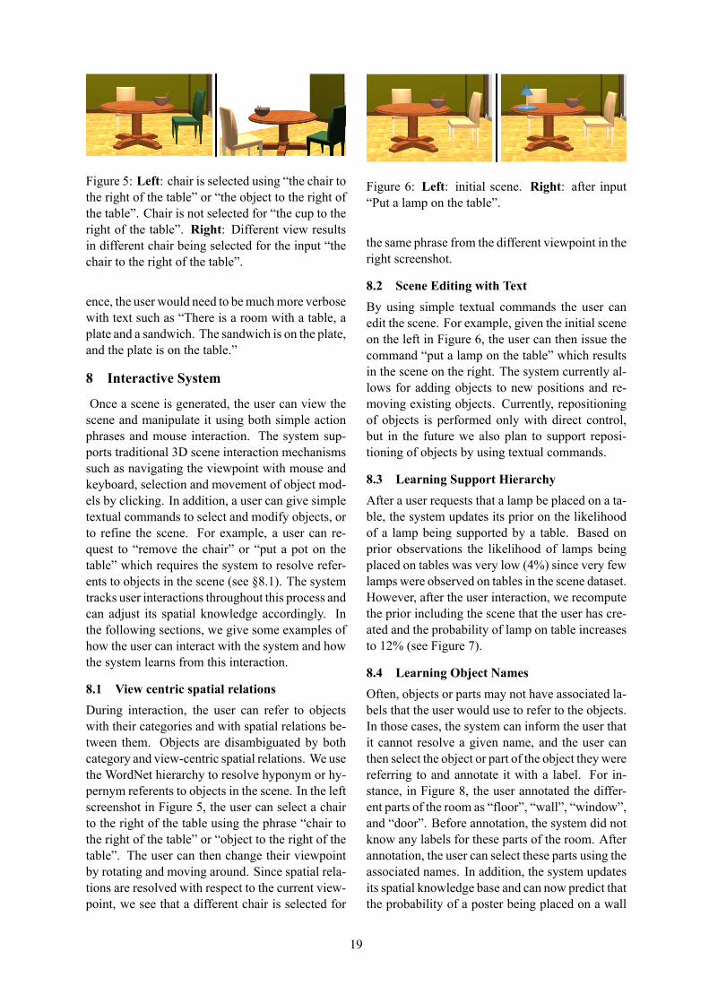
Figure 5: Left: chair is selected using “the chair tothe right of the table” or “the object to the right ofthe table”. Chair is not selected for “the cup to theright of the table”. Right: Different view resultsin different chair being selected for the input “thechair to the right of the table”.
ence, the user would need to bemuchmore verbosewith text such as “There is a room with a table, aplate and a sandwich. The sandwich is on the plate,and the plate is on the table.”
8 Interactive System
Once a scene is generated, the user can view thescene and manipulate it using both simple actionphrases and mouse interaction. The system sup-ports traditional 3D scene interaction mechanismssuch as navigating the viewpoint with mouse andkeyboard, selection and movement of object mod-els by clicking. In addition, a user can give simpletextual commands to select and modify objects, orto refine the scene. For example, a user can re-quest to “remove the chair” or “put a pot on thetable” which requires the system to resolve refer-ents to objects in the scene (see §8.1). The systemtracks user interactions throughout this process andcan adjust its spatial knowledge accordingly. Inthe following sections, we give some examples ofhow the user can interact with the system and howthe system learns from this interaction.
8.1 View centric spatial relationsDuring interaction, the user can refer to objectswith their categories and with spatial relations be-tween them. Objects are disambiguated by bothcategory and view-centric spatial relations. We usethe WordNet hierarchy to resolve hyponym or hy-pernym referents to objects in the scene. In the leftscreenshot in Figure 5, the user can select a chairto the right of the table using the phrase “chair tothe right of the table” or “object to the right of thetable”. The user can then change their viewpointby rotating and moving around. Since spatial rela-tions are resolved with respect to the current view-point, we see that a different chair is selected for
Figure 6: Left: initial scene. Right: after input“Put a lamp on the table”.
the same phrase from the different viewpoint in theright screenshot.
8.2 Scene Editing with TextBy using simple textual commands the user canedit the scene. For example, given the initial sceneon the left in Figure 6, the user can then issue thecommand “put a lamp on the table” which resultsin the scene on the right. The system currently al-lows for adding objects to new positions and re-moving existing objects. Currently, repositioningof objects is performed only with direct control,but in the future we also plan to support reposi-tioning of objects by using textual commands.
8.3 Learning Support HierarchyAfter a user requests that a lamp be placed on a ta-ble, the system updates its prior on the likelihoodof a lamp being supported by a table. Based onprior observations the likelihood of lamps beingplaced on tables was very low (4%) since very fewlamps were observed on tables in the scene dataset.However, after the user interaction, we recomputethe prior including the scene that the user has cre-ated and the probability of lamp on table increasesto 12% (see Figure 7).
8.4 Learning Object NamesOften, objects or parts may not have associated la-bels that the user would use to refer to the objects.In those cases, the system can inform the user thatit cannot resolve a given name, and the user canthen select the object or part of the object they werereferring to and annotate it with a label. For in-stance, in Figure 8, the user annotated the differ-ent parts of the room as “floor”, “wall”, “window”,and “door”. Before annotation, the system did notknow any labels for these parts of the room. Afterannotation, the user can select these parts using theassociated names. In addition, the system updatesits spatial knowledge base and can now predict thatthe probability of a poster being placed on a wall
19
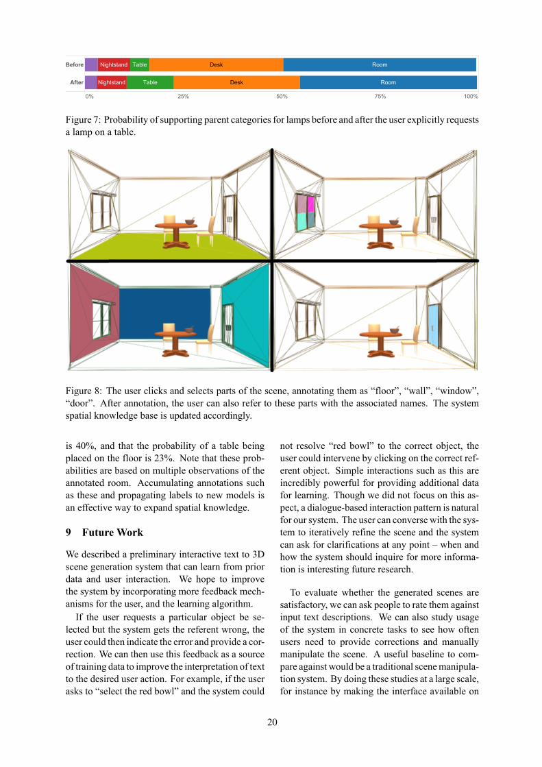
0% 25% 50% 75% 100%
Before
After
Nightstand
Nightstand
Room
Room
Table
Table
Desk
Desk
Figure 7: Probability of supporting parent categories for lamps before and after the user explicitly requestsa lamp on a table.
Figure 8: The user clicks and selects parts of the scene, annotating them as “floor”, “wall”, “window”,“door”. After annotation, the user can also refer to these parts with the associated names. The systemspatial knowledge base is updated accordingly.
is 40%, and that the probability of a table beingplaced on the floor is 23%. Note that these prob-abilities are based on multiple observations of theannotated room. Accumulating annotations suchas these and propagating labels to new models isan effective way to expand spatial knowledge.
9 Future Work
We described a preliminary interactive text to 3Dscene generation system that can learn from priordata and user interaction. We hope to improvethe system by incorporating more feedback mech-anisms for the user, and the learning algorithm.If the user requests a particular object be se-
lected but the system gets the referent wrong, theuser could then indicate the error and provide a cor-rection. We can then use this feedback as a sourceof training data to improve the interpretation of textto the desired user action. For example, if the userasks to “select the red bowl” and the system could
not resolve “red bowl” to the correct object, theuser could intervene by clicking on the correct ref-erent object. Simple interactions such as this areincredibly powerful for providing additional datafor learning. Though we did not focus on this as-pect, a dialogue-based interaction pattern is naturalfor our system. The user can converse with the sys-tem to iteratively refine the scene and the systemcan ask for clarifications at any point – when andhow the system should inquire for more informa-tion is interesting future research.
To evaluate whether the generated scenes aresatisfactory, we can ask people to rate them againstinput text descriptions. We can also study usageof the system in concrete tasks to see how oftenusers need to provide corrections and manuallymanipulate the scene. A useful baseline to com-pare against would be a traditional scenemanipula-tion system. By doing these studies at a large scale,for instance by making the interface available on
20
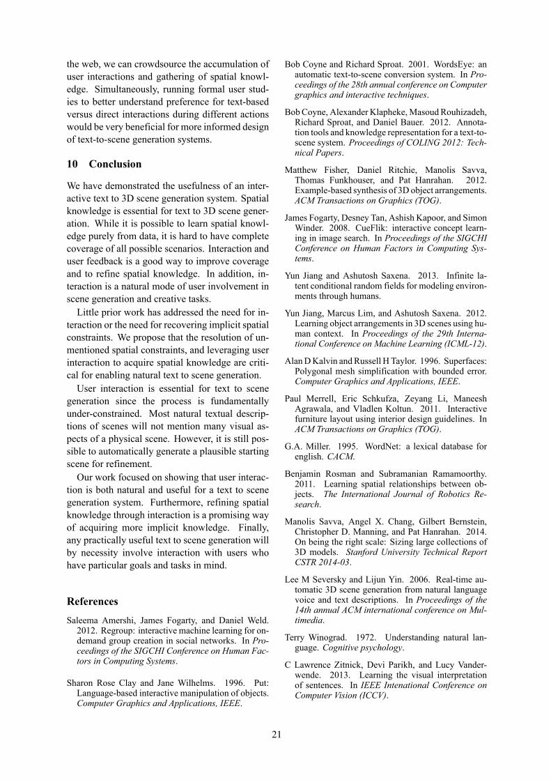
the web, we can crowdsource the accumulation ofuser interactions and gathering of spatial knowl-edge. Simultaneously, running formal user stud-ies to better understand preference for text-basedversus direct interactions during different actionswould be very beneficial for more informed designof text-to-scene generation systems.
10 Conclusion
We have demonstrated the usefulness of an inter-active text to 3D scene generation system. Spatialknowledge is essential for text to 3D scene gener-ation. While it is possible to learn spatial knowl-edge purely from data, it is hard to have completecoverage of all possible scenarios. Interaction anduser feedback is a good way to improve coverageand to refine spatial knowledge. In addition, in-teraction is a natural mode of user involvement inscene generation and creative tasks.Little prior work has addressed the need for in-
teraction or the need for recovering implicit spatialconstraints. We propose that the resolution of un-mentioned spatial constraints, and leveraging userinteraction to acquire spatial knowledge are criti-cal for enabling natural text to scene generation.User interaction is essential for text to scene
generation since the process is fundamentallyunder-constrained. Most natural textual descrip-tions of scenes will not mention many visual as-pects of a physical scene. However, it is still pos-sible to automatically generate a plausible startingscene for refinement.Our work focused on showing that user interac-
tion is both natural and useful for a text to scenegeneration system. Furthermore, refining spatialknowledge through interaction is a promising wayof acquiring more implicit knowledge. Finally,any practically useful text to scene generation willby necessity involve interaction with users whohave particular goals and tasks in mind.
ReferencesSaleema Amershi, James Fogarty, and Daniel Weld.
2012. Regroup: interactive machine learning for on-demand group creation in social networks. In Pro-ceedings of the SIGCHI Conference on Human Fac-tors in Computing Systems.
Sharon Rose Clay and Jane Wilhelms. 1996. Put:Language-based interactive manipulation of objects.Computer Graphics and Applications, IEEE.
Bob Coyne and Richard Sproat. 2001. WordsEye: anautomatic text-to-scene conversion system. In Pro-ceedings of the 28th annual conference on Computergraphics and interactive techniques.
BobCoyne, Alexander Klapheke,MasoudRouhizadeh,Richard Sproat, and Daniel Bauer. 2012. Annota-tion tools and knowledge representation for a text-to-scene system. Proceedings of COLING 2012: Tech-nical Papers.
Matthew Fisher, Daniel Ritchie, Manolis Savva,Thomas Funkhouser, and Pat Hanrahan. 2012.Example-based synthesis of 3D object arrangements.ACM Transactions on Graphics (TOG).
James Fogarty, Desney Tan, Ashish Kapoor, and SimonWinder. 2008. CueFlik: interactive concept learn-ing in image search. In Proceedings of the SIGCHIConference on Human Factors in Computing Sys-tems.
Yun Jiang and Ashutosh Saxena. 2013. Infinite la-tent conditional random fields for modeling environ-ments through humans.
Yun Jiang, Marcus Lim, and Ashutosh Saxena. 2012.Learning object arrangements in 3D scenes using hu-man context. In Proceedings of the 29th Interna-tional Conference on Machine Learning (ICML-12).
AlanDKalvin andRussell HTaylor. 1996. Superfaces:Polygonal mesh simplification with bounded error.Computer Graphics and Applications, IEEE.
Paul Merrell, Eric Schkufza, Zeyang Li, ManeeshAgrawala, and Vladlen Koltun. 2011. Interactivefurniture layout using interior design guidelines. InACM Transactions on Graphics (TOG).
G.A. Miller. 1995. WordNet: a lexical database forenglish. CACM.
Benjamin Rosman and Subramanian Ramamoorthy.2011. Learning spatial relationships between ob-jects. The International Journal of Robotics Re-search.
Manolis Savva, Angel X. Chang, Gilbert Bernstein,Christopher D. Manning, and Pat Hanrahan. 2014.On being the right scale: Sizing large collections of3D models. Stanford University Technical ReportCSTR 2014-03.
Lee M Seversky and Lijun Yin. 2006. Real-time au-tomatic 3D scene generation from natural languagevoice and text descriptions. In Proceedings of the14th annual ACM international conference on Mul-timedia.
Terry Winograd. 1972. Understanding natural lan-guage. Cognitive psychology.
C Lawrence Zitnick, Devi Parikh, and Lucy Vander-wende. 2013. Learning the visual interpretationof sentences. In IEEE Intenational Conference onComputer Vision (ICCV).
21
Proceedings of the Workshop on Interactive Language Learning, Visualization, and Interfaces, pages 22–29,Baltimore, Maryland, USA, June 27, 2014. c©2014 Association for Computational Linguistics
Dynamic Wordclouds and Vennclouds for Exploratory Data Analysis
Glen CoppersmithHuman Language Technology Center of Excellence
Johns Hopkins [email protected]
Erin KellyDepartment of Defense
Abstract
The wordcloud is a ubiquitous visualiza-tion of human language, though it fallsshort when used for exploratory data anal-ysis. To address some of these shortcom-ings, we give the viewer explicit controlover the creation of the wordcloud, allow-ing them to interact with it in real time–a dynamic wordcloud. This allows itera-tive adaptation of the visualization to thedata and inference task at hand. We nextpresent a principled approach to visualiza-tion which highlights the similarities anddifferences between two sets of documents– a Venncloud. We make all the visual-ization code (primarily JavaScript) freelyavailable.
1 Introduction
A cornerstone of exploratory data analysis is visu-alization. Tremendous academic effort and engi-neering expertise has created and refined a myriadof visualizations available to the data explorer, yetthere still exists a paucity of options for visualizinglanguage data. While visualizing human languageis a broad subject, we apply Polya’s dictum, andexamine a pair of simpler questions for which westill lack an answer:
• (1) what is in this corpus of documents?
• (2) what is the relationship between thesetwo corpora of documents?
We assert that addressing these two questions isa step towards creating visualizations of humanlanguage more suitable for exploratory data anal-ysis. In order to create a meaningful visualiza-tion, one must understand the inference questionthe visualization is meant to inform (i.e., the rea-son for which (1) is being asked), so the appro-priate aspects of the data can be highlighted with
the aesthetics of the visualization. Different infer-ence questions require different aspects to be high-lighted, so we aim to create a maximally-flexible,yet simple and intuitive method to enable a userto explore the relevant aspects of their data, andadapt the visualization to their task at hand.
The primary contributions of this paper are:
• A visualization of language data tailored forexploratory data analysis, designed to exam-ine a single corpus (the dynamic wordcloud)and to compare two corpora (the Venncloud);
• The framing and analysis of the problem interms of the existing psychophysical litera-ture;
• Distributable JavaScript code, designed to besimple to use, adapt, and extend.
We base our visualizations on the wordcloud,which we deconstruct and analyze in §3 and §4.We then discuss the literature on wordclouds andrelevant psychophysical findings in §5, takingguidance from the practical and theoretical foun-dations explored there. We then draw heavily onsimilarities to more common and well understoodvisualizations to create a more useful version ofthe wordcloud. Question (1) is addressed in §7,and with only a small further expansion describedin §8, an approach to (2) becomes evident.
2 Motivating Inference Tasks
Exploratory data analysis on human language en-compasses a diverse set of language and infer-ence tasks, so we select the following subset fortheir variety. One task in line with question (1)is getting the general subject of a corpus, high-lighting content-bearing words. One might wantto examine a collection of social media missives,too numerous to read individually, perhaps to de-tect emerging news (Petrovic et al., 2013). Sepa-rately, author identification (or idiolect analysis)
22
attempts attribution of documents (e.g., Shake-speare’s plays or the Federalist papers) by com-paring the author’s writing style, focusing onstylistic and contentless words – for a review see(Juola, 2006). Further, some linguistic psycho-metric analysis depends on the relative distribu-tion of pronouns and other seemingly contentlesswords (Coppersmith et al., 2014a; Chung and Pen-nebaker, 2007).
Each of these questions involves some analy-sis of unigram statistics, but exactly what analy-sis differs significantly, thus no single wordcloudcan display all of them. Any static wordcloud isa single point in a distribution of possible word-clouds – one way of calculating statistics from theunderlying language and mapping those calcula-tions to the visual representation. Many such com-binations and mappings are available, and the opti-mal wordcloud, like the optimal plot, is a functionof the data and the inference task at hand. Thus,we enable the wordcloud viewer to adjust the rela-tionship between the aspects of the data and theaesthetics of the display, which allows them toview different points in the distribution of possi-ble wordclouds. The dynamic wordcloud was im-plicitly called for in (Rayson and Garside, 2000)since human expertise (specifically knowledge ofbroader contexts and common sense) is neededto separate meaningful and non-meaningful differ-ences in wordclouds. We enable this dynamic in-teraction between human and visualization in real-time with a simple user interface, requiring only amodicum more engineering than the creation of astatic wordcloud, though the depth of extra infor-mation conveyed is significant.
3 Wordcloud Aesthetics
We refer to each visual component of the visual-ization as an aesthetic (ala (Wickham, 2009)) –each aesthetic can convey some information to theviewer. For context, the aesthetics of a scatterplotinclude the x and y position, color, and size ofeach point. Some are best suited for ordinal data(e.g., font size), while others for categorical data(e.g., font color).
Ordinal data can be encoded by font size,the most prominent and noticeable to the viewer(Bateman et al., 2008). Likewise, the opacity(transparency) of the word is a prominent and or-dinal aesthetic. The order in which words are dis-played can convey a significant amount of infor-
mation as well, but using order in this fashion gen-erally constrains the use of x and y position.
Categorical data can be encoded by the colorof each word – both the foreground of the worditself and the background space that surrounds it(though that bandwidth is severely limited by hu-man perception). Likewise for font weight (bold-ness) and font decoration (italics and underlines).While font face itself could encode a categoricalvariable, making comparisons of all the other as-pects across font faces is likely to be at best unin-formative and at worst misleading.
4 Data Aspects
As the wordcloud has visual aesthetics that we cancontrol (§3), the data we need to model has aspectsthat we want to represent with those aesthetics.This aspect-to-aesthetic mapping is what makes auseful and informative visualization, and needs tobe flexible enough to allow it be used for a rangeof inference tasks.
For clarity, we define a word (w) as a uniqueset of characters and a word token (w) as a sin-gle usage of a word in a document. We can ob-serve multiple word tokens (w) of the same word(w) in a single document (d). For any document dwe represent the term frequency of w as tfd(w).Similarly, the inverse document frequency of was idf(w). A combination of tf and idf is oftenused to determine important words in a documentor corpus. We focus on tf and idf here, but this isjust an example of an ordinal value associated witha word, there are many other such word-ordinalpairings that are worth exploring (e.g., weights ina classifier).
The dynamic range (“scaling” in (Wickham,2009)) also needs to be considered, since the datahas a natural dynamic range – where meaningfuldifferences can be observed (unsurprisingly, thedefinition of meaningful depends on the inferencetask). Likewise, each aesthetic has a range of val-ues for which the users can perceive and differen-tiate (e.g., words in a font size too small are illeg-ible, those too large prevent other words from be-ing displayed; not all differences are perceptible).Mapping the relevant dynamic range of the datato the dynamic range of the visualization is at theheart of a good visualization, but to do this algo-rithmically for all possible inference tasks remainsa challenge. We, instead, enable the user to adjustthe dynamic range of the visualization explicitly.
23
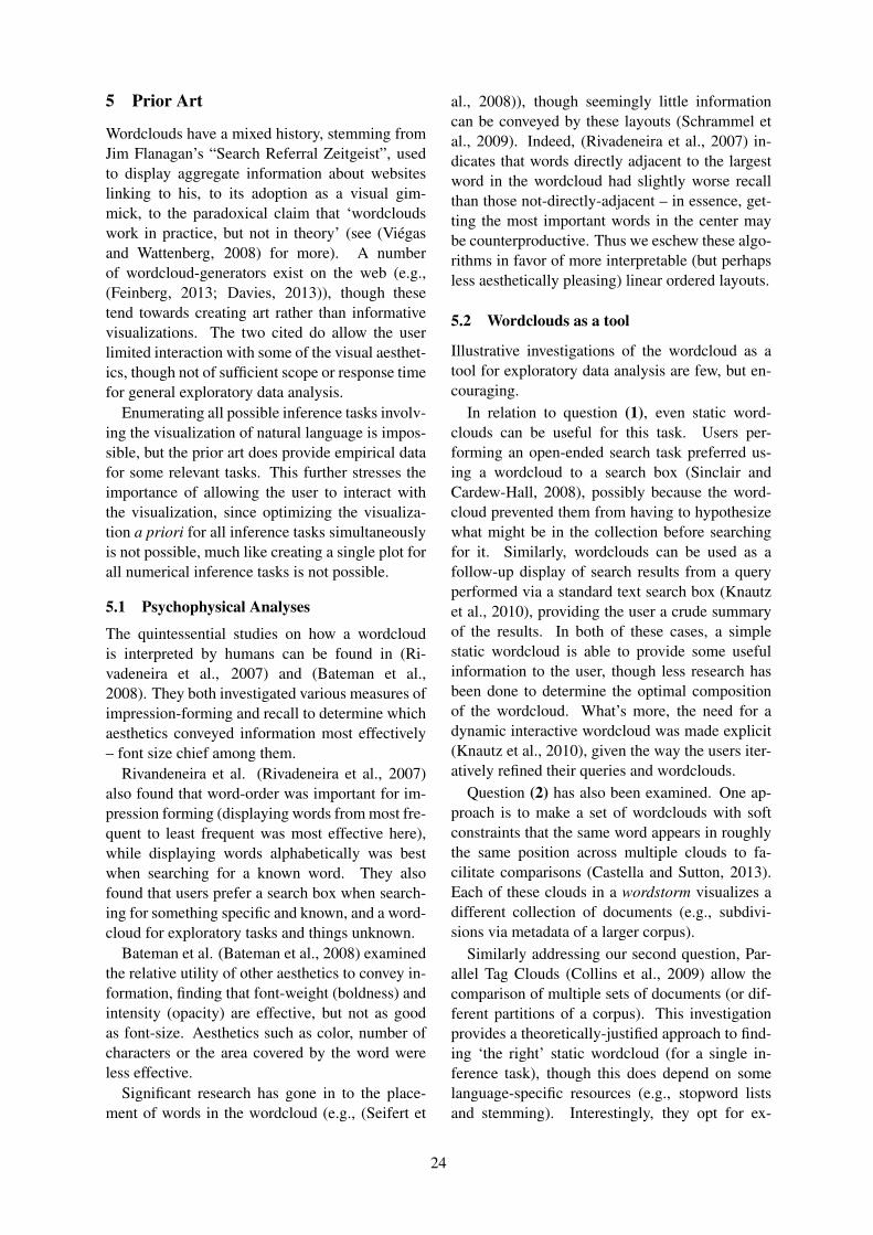
5 Prior Art
Wordclouds have a mixed history, stemming fromJim Flanagan’s “Search Referral Zeitgeist”, usedto display aggregate information about websiteslinking to his, to its adoption as a visual gim-mick, to the paradoxical claim that ‘wordcloudswork in practice, but not in theory’ (see (Viegasand Wattenberg, 2008) for more). A numberof wordcloud-generators exist on the web (e.g.,(Feinberg, 2013; Davies, 2013)), though thesetend towards creating art rather than informativevisualizations. The two cited do allow the userlimited interaction with some of the visual aesthet-ics, though not of sufficient scope or response timefor general exploratory data analysis.
Enumerating all possible inference tasks involv-ing the visualization of natural language is impos-sible, but the prior art does provide empirical datafor some relevant tasks. This further stresses theimportance of allowing the user to interact withthe visualization, since optimizing the visualiza-tion a priori for all inference tasks simultaneouslyis not possible, much like creating a single plot forall numerical inference tasks is not possible.
5.1 Psychophysical Analyses
The quintessential studies on how a wordcloudis interpreted by humans can be found in (Ri-vadeneira et al., 2007) and (Bateman et al.,2008). They both investigated various measures ofimpression-forming and recall to determine whichaesthetics conveyed information most effectively– font size chief among them.
Rivandeneira et al. (Rivadeneira et al., 2007)also found that word-order was important for im-pression forming (displaying words from most fre-quent to least frequent was most effective here),while displaying words alphabetically was bestwhen searching for a known word. They alsofound that users prefer a search box when search-ing for something specific and known, and a word-cloud for exploratory tasks and things unknown.
Bateman et al. (Bateman et al., 2008) examinedthe relative utility of other aesthetics to convey in-formation, finding that font-weight (boldness) andintensity (opacity) are effective, but not as goodas font-size. Aesthetics such as color, number ofcharacters or the area covered by the word wereless effective.
Significant research has gone in to the place-ment of words in the wordcloud (e.g., (Seifert et
al., 2008)), though seemingly little informationcan be conveyed by these layouts (Schrammel etal., 2009). Indeed, (Rivadeneira et al., 2007) in-dicates that words directly adjacent to the largestword in the wordcloud had slightly worse recallthan those not-directly-adjacent – in essence, get-ting the most important words in the center maybe counterproductive. Thus we eschew these algo-rithms in favor of more interpretable (but perhapsless aesthetically pleasing) linear ordered layouts.
5.2 Wordclouds as a tool
Illustrative investigations of the wordcloud as atool for exploratory data analysis are few, but en-couraging.
In relation to question (1), even static word-clouds can be useful for this task. Users per-forming an open-ended search task preferred us-ing a wordcloud to a search box (Sinclair andCardew-Hall, 2008), possibly because the word-cloud prevented them from having to hypothesizewhat might be in the collection before searchingfor it. Similarly, wordclouds can be used as afollow-up display of search results from a queryperformed via a standard text search box (Knautzet al., 2010), providing the user a crude summaryof the results. In both of these cases, a simplestatic wordcloud is able to provide some usefulinformation to the user, though less research hasbeen done to determine the optimal compositionof the wordcloud. What’s more, the need for adynamic interactive wordcloud was made explicit(Knautz et al., 2010), given the way the users iter-atively refined their queries and wordclouds.
Question (2) has also been examined. One ap-proach is to make a set of wordclouds with softconstraints that the same word appears in roughlythe same position across multiple clouds to fa-cilitate comparisons (Castella and Sutton, 2013).Each of these clouds in a wordstorm visualizes adifferent collection of documents (e.g., subdivi-sions via metadata of a larger corpus).
Similarly addressing our second question, Par-allel Tag Clouds (Collins et al., 2009) allow thecomparison of multiple sets of documents (or dif-ferent partitions of a corpus). This investigationprovides a theoretically-justified approach to find-ing ‘the right’ static wordcloud (for a single in-ference task), though this does depend on somelanguage-specific resources (e.g., stopword listsand stemming). Interestingly, they opt for ex-
24
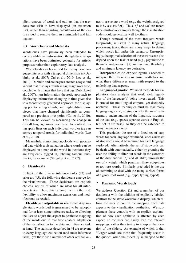
plicit removal of words and outliers that the userdoes not wish to have displayed (an exclusionlist), rather than adjusting calculations of the en-tire cloud to remove them in a principled and fairmanner.
5.3 Wordclouds and Metadata
Wordclouds have previously been extended toconvey additional information, though these adap-tations have been optimized generally for artisticpurposes rather than exploratory data analysis.
Wordclouds can been used to display how lan-guage interacts with a temporal dimension in (Du-binko et al., 2007; Cui et al., 2010; Lee et al.,2010). Dubinko and colleagues created a tag cloudvariant that displays trends in tag usage over time,coupled with images that have that tag (Dubinko etal., 2007). An information-theoretic approach todisplaying information changing in time gives riseto a theoretically grounded approach for display-ing pointwise tag clouds, and highlighting thosepieces that have changed significantly as com-pared to a previous time period (Cui et al., 2010).This can be viewed as measuring the change inoverall language usage over time. In contrast, us-ing spark lines on each individual word or tag canconvey temporal trends for individual words (Leeet al., 2010).
Meanwhile, combining tag clouds with geospa-tial data yields a visualization where words can bedisplayed on a map of the world in locations theyare frequently tagged in, labeling famous land-marks, for example (Slingsby et al., 2007).
6 Desiderata
In light of the diverse inference tasks (§2) andprior art (§5), the following desiderata emerge forthe visualization. These desiderata are explicitchoices, not all of which are ideal for all infer-ence tasks. Thus, chief among them is the first:flexibility to allow maximum extensions and mod-ifications as needed.
Flexible and adjustable in real time: Any sin-gle static wordcloud is guaranteed to be subopti-mal for at least some inference tasks, so allowingthe user to adjust the aspect-to-aesthetic mappingof the wordcloud in real time enables adaptationof the visualization to the data and inference taskat hand. The statistics described in §4 are relevantto every language collection (and most inferencetasks), yet there are a number of other ordinal val-
ues to associate a word (e.g., the weight assignedto it by a classifier). Thus, tf and idf are meantto be illustrative examples though the visualizationcode should generalize well to others.
Though removal of the most frequent words(stopwords) is useful in many natural languageprocessing tasks, there are many ways to definewhich words fall under this category. Unsurpris-ingly, the optimal selection of these words can alsodepend upon the task at hand (e.g., psychiatric v.thematic analysis as in §2), so maximum flexibilityand minimum latency are desirable.
Interpretable: An explicit legend is needed tointerpret the differences in visual aesthetics andwhat these differences mean with respect to theunderlying data aspects.
Language-Agnostic: We need methods for ex-ploratory data analysis that work well regard-less of the language(s) being investigated. Thisis crucial for multilingual corpora, yet decidedlynontrivial. These techniques must be maximallylanguage-agnostic, relying on only the most rudi-mentary understanding of the linguistic structureof the data (e.g., spaces separate words in English,but not in Chinese), so they can be extended tomany languages easily.
This precludes the use of a fixed set of stopwords for each language examined, since a new setof stopwords would be required for each languageexplored. Alternatively, the set of stopwords canbe dealt with automatically, either by granting theuser the ability to filter out words in the extremesof the distributions (tf and df alike) through theuse of a weight which penalizes these ubiquitousor too-rare words. Similarly precluded is the useof stemming to deal with the many surface formsof a given root word (e.g., type, typing, typed).
7 Dynamic Wordclouds
We address Question (1) and a number of ourdesiderata with the addition of explicitly labeledcontrols to the static wordcloud display, which al-lows the user to control the mapping from dataaspects to the visualization aesthetics. We sup-plement these controls with an explicit explana-tion of how each aesthetic is affected by eachaspect, so the user can easily read the relevantmappings, rather than trying to interpret the loca-tion of the sliders. An example of which is that“Larger words are those that frequently occur inthe query”, when the aspect tf is mapped to the
25
[X] entities commoncloud
tffilter
idffilter
sizecontrols
opacitycontrols
sortby
wordclouddescription
do notredraw
highlightkeywords
orioles at to for inbaltimore a game iand yankees of goon is this vs w/ o'sare it win with be i'mmy you that others newhave just 2 3 up 1 let's first so alltonight fans but out season we now get soxan time md series al baseball will about me notlike as 5 playoff lets from over was they if what 4 good nogreat year day one love back amp fan magic can east playoffs beat gtred sports rt today do going how last more place team games night blue
file:///Users/gcoppersmith/Desktop/dwc_dev/orioles.html
1 of 2 2/24/14, 4:36 PM
[X] entities commoncloud
tffilter
idffilter
sizecontrols
opacitycontrols
sortby
wordclouddescription
do notredraw
highlightkeywords
13 espn fox leads md ny report starusa buck chris glove mark move press14 gold hamilton jim third birds gonzalez jo september white homers rangers tigers 15 fallyankee sox yard al happen pick blue cc extra m oldcard closer hits tie tied face omg ravens says yahoo citysaying second starting stay ass manager players real lt threebout football left sunday sweep goes hey gets wild yanks adam jobnews times won't magic place innings 2013 base gt hr pitching doesfucking os rain 10 friday outs suck coming makes also check wearinghaha show through god los losing may always being keep 9 hate gotta looksmaking posted away free im life we're weekend call give little bar bring didn'tdoing least look stop thing top where giants long photo record johnson leaguemost thank tv ? please proud walk wish 2012 any end every hell post samebecause many pitch said its new runs everyone excited field finally bullpen let redyes believe fun made these boys hit into those against mlb race i'll teams amazing sayw years another people 1st both postseason wait before 8 looking loss him lead man shitfeel inning damn oh 7 baby i've again should bad then thanks two wins nice much that'swinning yankees than gonna playing tickets yeah awesome beat why division lol wowcongrats lost ready lose us big could never even fuck our want since ball ever happy start ambetter make run hope think only over he were getting has sports really his u work 6 next wonchecked chicago did them some after well best tomorrow watch take their when had too orioles there angames world need who 0 stadium clinch your been down love don't way by east or know off play would 4more o's it's no can't rt playoffs right as still how can back here playoff 1 5 year 3 night watching team do lastone amp got day series home see come great today from like 2 will fan going what pic they about time good lets firstseason if get was tonight we not fans let's all me baseball out now up just so but have be win you that with i'm it are myothers this is washington on vs of w/ go i and
file:///Users/gcoppersmith/Desktop/dwc_dev/orioles.html
1 of 1 2/24/14, 4:35 PM
[X] entities commoncloud
tffilter
idffilter
sizecontrols
opacitycontrols
sortby
wordclouddescription
do notredraw
highlightkeywords
0 1 1st 2 2012 3 4 5 6 7 ? a about after again against al all amp an and are as
at back baltimore baseball be beat been best better
big birds blue buck but by can can't card checked chicago come could
day did do don't down east espn even ever fan fans first for from fuck gamegames get go going gonna good got great gt had has have he here his hit home how i i'mif in inning is it it's johnson just keep know last lead let's lets like lol lose love
magic make mark md me mlb more my need new news next
night no not now o's of off on one only or orioles others our
out over photo pic place play playoff playoffs post postseason rangersravens really red report right rt run season see series should since so some
sox sports start still take team than that their them there they think this tied time
times to today tomorrow tonight two up vs w/ was watch watching way we well were
what when white who why wild will win with won world would yahooyankees yanks year years you your
file:///Users/gcoppersmith/Desktop/dwc_dev/orioles.html
1 of 1 2/24/14, 4:37 PMFigure 1: Three example settings of the dynamic wordcloud for the same set of tweets containing “Orioles”. Left: sizereflects tf , sorted by tf ; Center: size reflects idf , sorted by idf ; Right: size reflects tf*idf , sorted alphabetically.
aesthetic font-size (and this description is tied tothe appropriate sliders so it updates as the slid-ers are changed). The manipulation of the visu-alization in real time allows us to take advantageof the human’s adept visual change-detection tohighlight and convey the differences between set-tings (or a range of settings), even subtle ones.
The data aspects from §4 are precomputed andmapped to the aesthetics from §3 in a JavaScriptvisualization displayed in a standard web browser.This visualization enables the user to manipulatethe aspect-to-aesthetic mapping via an intuitiveset of sliders and buttons, responsive in real time.The sliders are roughly segmented into three cat-egories: those that control which words are dis-played, those that control how size is calculated,and those that control how opacity is calculated.The buttons control the order in which words ap-pear.
One set of sliders controls which words aredisplayed by examining the frequency and rar-ity of the words. We define the range τFreq =[tmin
Freq, tmaxFreq] as the range of tf values for words to
be displayed (i.e., tf(w) ∈ τFreq). The viewer isgranted a range slider to manipulate both tmin
Freq andtmaxFreq to eliminate words from the extremes of the
distribution. Similarly for df and τRarity. Thosewords that fall outside τFreq or τRarity are not dis-played. Importantly, tf is computed from the cur-rent corpus displayed while df is computed over amuch larger collection (in our running examples,all the works of Shakespeare or all the tweets forthe last 6 months). Those with high df or hightf are often stopwords, those with low tf and lowdf are often rare, sometimes too rare to get goodestimates of tf or idf (e.g., names).
A second set of sliders controls the mapping be-tween aspects and aesthetics for each individualword. Each aesthetic has a weight for the impor-tance of rarity (γRarity) and the importance of fre-quency (γFreq), corresponding to the current val-ues of their respective slider (each in the range[0, 1]). For size, we compute a weight attributedto each data aspect:
ωFreq(w) = (1− γFreq) + γFreqtf(w)
and similarly for Rarity.In both cases, the aesthetic’s value is computed
via an equation similar to the following:
a(w) = ωFreq(w)ωRarity(w)γRangeb
where a(w) is either font size or opacity, and bis some base value of the aesthetic (scaled by adynamic range slider, γRange) and the weights forfrequency and rarity of the word. In this manner,the weights are multiplicative, so interactions be-tween the variables (e.g., tf*idf ) are apparent.
Though unigram statistics are informative, see-ing the unigrams in context is also important formany inference tasks. To enable this, we use reser-voir sampling (Vitter, 1985) to maintain a repre-sentative sample of the observed occurrences ofeach word in context, which the user can view byclicking on the word in the wordcloud display.
Examples of the dynamic wordcloud in varioussettings can be found in Figure 1, using a set oftweets containing “Orioles”. The left wordcloudhas tf mapped to size, the center with idf mappedto size, and the right with both high tf and highidf mapped to size. We only manipulate the sizeaesthetic, since the opacity aesthetic is sometimeshard to interpret in print. To fit the wordclouds
26
to the small format, various values for τFreq andτRarity are employed, and order is varied – theleft is ordered in descending order in terms of fre-quency, the center is ordered in descending orderin terms of rarity, and the right is in alphabeticalorder.
8 Vennclouds
Question (2) – “how are these corpora related” re-quires only a single change to the dynamic sin-gle wordcloud described in §7. We refer to twocorpora, left and right, which we abbreviate Land R (perhaps a set of tweets containing “Ori-oles” for left and those containing “Nationals” forright as in Figure 2). For the right documents, letR = {d1, ..., dnR} so |R| = nR and let TR be thetotal number of tokens in all the documents in R
TR =∑d∈R
|Td|
We separate the wordcloud display into three re-gions, one devoted to words most closely associ-ated with R, one devoted to words most closelyassociated with L, and one for words that shouldbe associated with both. “Association” here can bedefined in a number of ways, but for the nonce wedefine it as the probability of occurrence in thatcorpus – essentially term frequency, normalizedby corpus length. Normalizing by length is re-quired to prevent bias incurred when the corporaare different sizes (TL 6= TR). Specifically, wedefine the number of times w occurs in left (tf ) as
tfL(w) =∑di∈L
T (w, di)
and this quantity normalized by the number of to-kens in L,
tfL(w) = tfL(w)/TL
and this quantity as it relates to the term frequencyof this w in both corpora
tfL|R(w) =tfL(w)
tfL(w) + tfR(w)
Each word is only displayed once in the Ven-ncloud (see Figure 2, so if a word (w) only occursin R, it is always present in the right region, andlikewise for L and left. If w is in both L and R,we examine the proportion of documents in eachthat w is in and use this to determine in which re-gion it should be displayed. In order to deal with
Figure 2: Three example Vennclouds, with tweets contain-ing “Orioles” on the left, “Nationals” on the right, and com-mon words in the middle. From top to bottom we allow pro-gressively larger common clouds. The large common wordsmake sense – both teams played a Chicago team and madethe playoffs in the time covered by these corpora.
the cases where w occurs in approximately similarproportions of left and right documents, we havea center region (in the center in Figure 2). Wedefine a threshold (τCommon) to concretely define“approximately similar”. Specifically,
• if tfR(w) = 0, w is displayed in left.
• if tfL(w) = 0, w is displayed in right.
• if tfR(w) > 0 and tfL(w) > 0,
– if tfR|L(w) > tfL|R(w) + τCommon, wis displayed in right.
– if tfL|R(w) > tfR|L(w) + τCommon, wis displayed in left.
– Otherwise, w is displayed in center.
The user is given a slider to control τCommon, al-lowing them to determine what value of “approx-imately similar” best fits the data and their task athand.
9 Anecdotal Evaluation
We have not yet done a proper psychophysicalevaluation of the utility of dynamic wordclouds
27
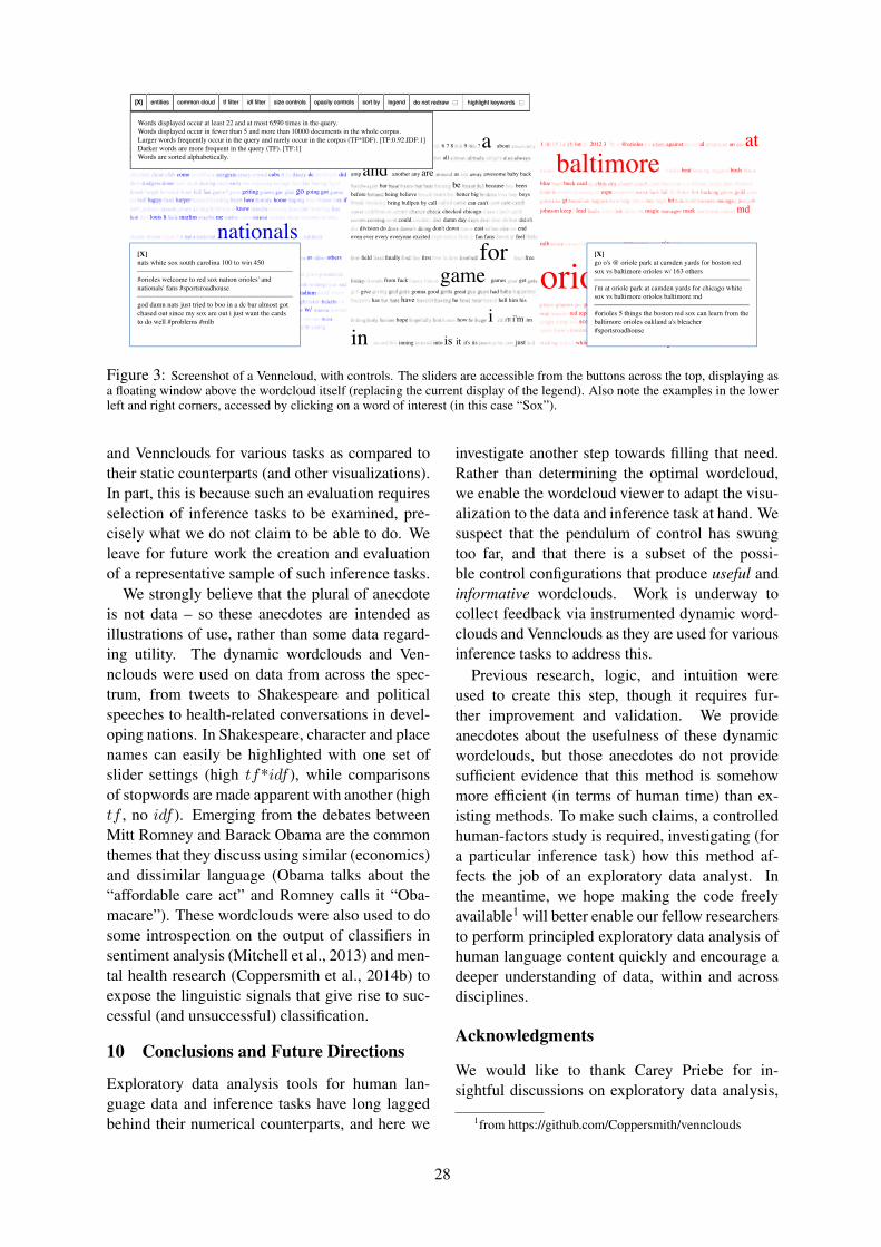
[X][X] entitiesentities common cloudcommon cloud tf filtertf filter idf filteridf filter size controlssize controls opacity controlsopacity controls sort bysort by legendlegend do not redraw do not redraw highlight keywords highlight keywords
@ @nationals am baseball best bryce but
cardinals cards clinchcome cubs dc did
getting go going got here home if
know louis lt marlins me
nationals nats nl not or others
park philadelphia phillies pic
see st stadium strasburg teddy
today too u w/ was washington watching well werth
work
0 2 4 5 6 7 8 9 ? a about
after again all
amp and another any are as awesome baby back
bar be because beenbefore being believe better big boys
bring bullpen by call can can't checked chicago
could damn day division do don't down east end
even ever every everyone excited fan fans feel
field finally first for free
from fuck game games get
give gonna good great had has have he hell him his
hope how i i'll i'm im
in inning into is it it's its just
last league let let's lets life like littlelol long look looking lose losing loss love made
make man many
more most much my need
next night no now of off oh on one only
our out pitch playplaying playoff playoffs please postseason proud
ready really right rt run runs saidsay season series should since so some
start still take team than
thank thanks that that's their them then there these they thing
think this those time to tomorrow tonight two
up vs wait want watch way we were what when where
who why will win winning wish with won worldwould yeah year yes you your
1 1st 2012 3 @orioles against al an atbaltimore beat birds
blue buck card espn
gt hit
johnson keep lead magic mark md
mlb new news o's
orioles over photo place
post rangers ravensred report
sox sports tied
white wild yahoo yankees yanks years
Words displayed occur at least 22 and at most 6590 times in the query.Words displayed occur in fewer than 5 and more than 10000 documents in the whole corpus.Larger words frequently occur in the query and rarely occur in the corpus (TF*IDF). [TF:0.92,IDF:1]Darker words are more frequent in the query (TF). [TF:1]Words are sorted alphabetically.
[X]go o's @ oriole park at camden yards for boston redsox vs baltimore orioles w/ 163 others
i'm at oriole park at camden yards for chicago whitesox vs baltimore orioles baltimore md
#orioles 5 things the boston red sox can learn from thebaltimore orioles oakland a's bleacher#sportsroadhouse
[X]nats white sox south carolina 100 to win 450
#orioles welcome to red sox nation orioles' andnationals' fans #sportsroadhouse
god damn nats just tried to boo in a dc bar almost gotchased out since my sox are out i just want the cardsto do well #problems #mlb
file:///Users/gcoppersmith/src/dwc_dev/nats_v_orioles.html
1 of 1 4/24/14, 9:53 AM
Figure 3: Screenshot of a Venncloud, with controls. The sliders are accessible from the buttons across the top, displaying asa floating window above the wordcloud itself (replacing the current display of the legend). Also note the examples in the lowerleft and right corners, accessed by clicking on a word of interest (in this case “Sox”).
and Vennclouds for various tasks as compared totheir static counterparts (and other visualizations).In part, this is because such an evaluation requiresselection of inference tasks to be examined, pre-cisely what we do not claim to be able to do. Weleave for future work the creation and evaluationof a representative sample of such inference tasks.
We strongly believe that the plural of anecdoteis not data – so these anecdotes are intended asillustrations of use, rather than some data regard-ing utility. The dynamic wordclouds and Ven-nclouds were used on data from across the spec-trum, from tweets to Shakespeare and politicalspeeches to health-related conversations in devel-oping nations. In Shakespeare, character and placenames can easily be highlighted with one set ofslider settings (high tf*idf ), while comparisonsof stopwords are made apparent with another (hightf , no idf ). Emerging from the debates betweenMitt Romney and Barack Obama are the commonthemes that they discuss using similar (economics)and dissimilar language (Obama talks about the“affordable care act” and Romney calls it “Oba-macare”). These wordclouds were also used to dosome introspection on the output of classifiers insentiment analysis (Mitchell et al., 2013) and men-tal health research (Coppersmith et al., 2014b) toexpose the linguistic signals that give rise to suc-cessful (and unsuccessful) classification.
10 Conclusions and Future Directions
Exploratory data analysis tools for human lan-guage data and inference tasks have long laggedbehind their numerical counterparts, and here we
investigate another step towards filling that need.Rather than determining the optimal wordcloud,we enable the wordcloud viewer to adapt the visu-alization to the data and inference task at hand. Wesuspect that the pendulum of control has swungtoo far, and that there is a subset of the possi-ble control configurations that produce useful andinformative wordclouds. Work is underway tocollect feedback via instrumented dynamic word-clouds and Vennclouds as they are used for variousinference tasks to address this.
Previous research, logic, and intuition wereused to create this step, though it requires fur-ther improvement and validation. We provideanecdotes about the usefulness of these dynamicwordclouds, but those anecdotes do not providesufficient evidence that this method is somehowmore efficient (in terms of human time) than ex-isting methods. To make such claims, a controlledhuman-factors study is required, investigating (fora particular inference task) how this method af-fects the job of an exploratory data analyst. Inthe meantime, we hope making the code freelyavailable1 will better enable our fellow researchersto perform principled exploratory data analysis ofhuman language content quickly and encourage adeeper understanding of data, within and acrossdisciplines.
Acknowledgments
We would like to thank Carey Priebe for in-sightful discussions on exploratory data analysis,
1from https://github.com/Coppersmith/vennclouds
28
Aleksander Yelskiy, Jacqueline Aguilar, KristyHollingshead for their analysis, comments, andimprovements on early versions, and AinsleyR. Coppersmith for permitting this research toprogress in her early months.
ReferencesScott Bateman, Carl Gutwin, and Miguel Nacenta.
2008. Seeing things in the clouds: the effect of vi-sual features on tag cloud selections. In Proceedingsof the nineteenth ACM conference on Hypertext andhypermedia, pages 193–202. ACM.
Quim Castella and Charles A. Sutton. 2013. Wordstorms: Multiples of word clouds for visual compar-ison of documents. CoRR, abs/1301.0503.
Cindy Chung and James W Pennebaker. 2007. Thepsychological functions of function words. Socialcommunication, pages 343–359.
Christopher Collins, Fernanda B Viegas, and MartinWattenberg. 2009. Parallel tag clouds to exploreand analyze faceted text corpora. In Visual Analyt-ics Science and Technology, 2009. VAST 2009. IEEESymposium on, pages 91–98. IEEE.
Glen Coppersmith, Mark Dredze, and Craig Harman.2014a. Quantifying mental health signals in twitter.In Proceedings of ACL Workshop on ComputationalLinguistics and Clinical Psychology. Association forComputational Linguistics.
Glen Coppersmith, Craig Harman, and Mark Dredze.2014b. Measuring post traumatic stress disorder inTwitter. In Proceedings of the International AAAIConference on Weblogs and Social Media (ICWSM).
Weiwei Cui, Yingcai Wu, Shixia Liu, Furu Wei,Michelle X Zhou, and Huamin Qu. 2010. Contextpreserving dynamic word cloud visualization. InPacific Visualization Symposium (PacificVis), 2010IEEE, pages 121–128. IEEE.
Jason Davies. 2013. Wordcloud generator using d3,April.
Micah Dubinko, Ravi Kumar, Joseph Magnani, Jas-mine Novak, Prabhakar Raghavan, and AndrewTomkins. 2007. Visualizing tags over time. ACMTransactions on the Web (TWEB), 1(2):7.
Jason Feinberg. 2013. Wordle, April.
Patrick Juola. 2006. Authorship attribution. Founda-tions and Trends in information Retrieval, 1(3):233–334.
Kathrin Knautz, Simone Soubusta, and Wolfgang GStock. 2010. Tag clusters as information retrievalinterfaces. In System Sciences (HICSS), 2010 43rdHawaii International Conference on, pages 1–10.IEEE.
Bongshin Lee, Nathalie Henry Riche, Amy K Karl-son, and Sheelagh Carpendale. 2010. Spark-clouds: Visualizing trends in tag clouds. Visualiza-tion and Computer Graphics, IEEE Transactions on,16(6):1182–1189.
Margaret Mitchell, Jacqueline Aguilar, Theresa Wil-son, and Benjamin Van Durme. 2013. Open domaintargeted sentiment. In Proceedings of the 2013 Con-ference on Empirical Methods in Natural LanguageProcessing, pages 1643–1654. Association for Com-putational Linguistics.
Sasa Petrovic, Miles Osborne, Richard McCreadie,Craig Macdonald, Iadh Ounis, and Luke Shrimpton.2013. Can twitter replace newswire for breakingnews. In Seventh International AAAI Conference onWeblogs and Social Media.
Paul Rayson and Roger Garside. 2000. Comparingcorpora using frequency profiling. In Proceedingsof the workshop on Comparing Corpora, pages 1–6.Association for Computational Linguistics.
AW Rivadeneira, Daniel M Gruen, Michael J Muller,and David R Millen. 2007. Getting our head in theclouds: toward evaluation studies of tagclouds. InProceedings of the SIGCHI conference on Humanfactors in computing systems, pages 995–998. ACM.
Johann Schrammel, Michael Leitner, and ManfredTscheligi. 2009. Semantically structured tagclouds: an empirical evaluation of clustered presen-tation approaches. In Proceedings of the 27th inter-national conference on Human factors in computingsystems, pages 2037–2040. ACM.
Christin Seifert, Barbara Kump, Wolfgang Kienreich,Gisela Granitzer, and Michael Granitzer. 2008. Onthe beauty and usability of tag clouds. In Informa-tion Visualisation, 2008. IV’08. 12th InternationalConference, pages 17–25. IEEE.
James Sinclair and Michael Cardew-Hall. 2008. Thefolksonomy tag cloud: when is it useful? Journal ofInformation Science, 34(1):15–29.
Aidan Slingsby, Jason Dykes, Jo Wood, and KeithClarke. 2007. Interactive tag maps and tagclouds for the multiscale exploration of large spatio-temporal datasets. In Information Visualization,2007. IV’07. 11th International Conference, pages497–504. IEEE.
Fernanda B Viegas and Martin Wattenberg. 2008.Timelines tag clouds and the case for vernacular vi-sualization. interactions, 15(4):49–52.
Jeffrey S Vitter. 1985. Random sampling with a reser-voir. ACM Transactions on Mathematical Software(TOMS), 11(1):37–57.
Hadley Wickham. 2009. ggplot2: elegant graphics fordata analysis. Springer Publishing Company, Incor-porated.
29
Proceedings of the Workshop on Interactive Language Learning, Visualization, and Interfaces, pages 30–33,Baltimore, Maryland, USA, June 27, 2014. c©2014 Association for Computational Linguistics
Active Learning with Constrained Topic ModelYi Yang
Northwestern [email protected]
Shimei PanIBM T. J. Watson Research Center
Doug DowneyNorthwestern University
Kunpeng ZhangUniversity of Illinois at Chicago
Abstract
Latent Dirichlet Allocation (LDA) is a topicmodeling tool that automatically discoverstopics from a large collection of documents.It is one of the most popular text analysistools currently in use. In practice however,the topics discovered by LDA do not al-ways make sense to end users. In this ex-tended abstract, we propose an active learn-ing framework that interactively and itera-tively acquires user feedback to improve thequality of learned topics. We conduct exper-iments to demonstrate its effectiveness withsimulated user input on a benchmark dataset.
1 Introduction
Statistical topic models such as Latent Dirichlet Al-location (LDA) (Blei et al., 2003) provide powerfultools for uncovering hidden thematic patterns in textand are useful for representing and summarizing thecontents of large document collections. However,when using topic models in practice, users often faceone critical problem: topics discovered by the modeldo not always make sense. A topic may contain the-matically unrelated words. Moreover, two thematicrelated words may appear in different topics. Thisis mainly because the objective function optimizedby LDA may not reflect human judgments of topicquality (Boyd-Graber et al., 2009).
Potentially, we can solve these problems by incor-porating additional user guidance or domain knowl-edge in topic modeling. With standard LDA how-ever, it is impossible for users to interact with themodel and provide feedback. (Hu et al., 2011) pro-posed an interactive topic modeling framework thatallows users to add word must-links. However, ithas several limitations. Since the vocabulary size ofa large document collection can be very large, usersmay need to annotate a large number of word con-straints for this method to be effective. Thus, thisprocess can be very tedious. More importantly, it
cannot handle polysemes. For example, the word“pound” can refer to either a currency or a unit ofmass. If a user adds a must-link between “pound”and another financial term, then he/she cannot adda must-link between “pound” and any measurementterms. Since word must-links are added withoutcontext, there is no way to disambiguate them. As aresult, word constraints frequently are not as effec-tive as document constraints.
Active learning (Settles, 2010) provides a use-ful framework which allows users to iteratively givefeedback to the model to improve its quality. In gen-eral, with the same amount of human labeling, ac-tive learning often results in a better model than thatlearned by an off-line method.
In this extended abstract, we propose an activelearning framework for LDA. It is based on a newconstrained topic modeling framework which is ca-pable of handling pairwise document constraints.We present several design choices and the pros andcons of each choice. We also conduct simulated ex-periments to demonstrate the effectiveness of the ap-proach.
2 Active Learning With Constrained TopicModeling
In this section, we first summarize our work on con-strained topic modeling. Then, we introduce anactive topic learning framework that employs con-strained topic modeling.
In LDA, a document’s topic distribution ~θ isdrawn from a Dirichlet distribution with prior ~α.A simple and commonly used Dirichlet distributionuses a symmetric ~α prior. However, (Wallach et al.,2009) has shown that an asymmetric Dirichlet priorover the document-topic distributions ~θ and a sym-metric Dirichlet prior over the topic-word distribu-tions ~φ yield significant improvements in model per-formance. Our constrained topic model uses asym-metric priors to encode constraints.
To incorporate user feedback, we focus on two
130
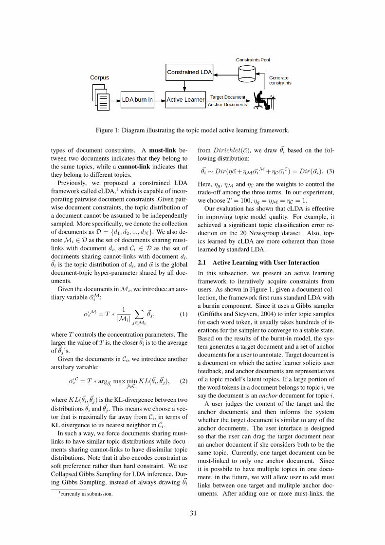
Figure 1: Diagram illustrating the topic model active learning framework.
types of document constraints. A must-link be-tween two documents indicates that they belong tothe same topics, while a cannot-link indicates thatthey belong to different topics.
Previously, we proposed a constrained LDAframework called cLDA,1 which is capable of incor-porating pairwise document constraints. Given pair-wise document constraints, the topic distribution ofa document cannot be assumed to be independentlysampled. More specifically, we denote the collectionof documents as D = {d1, d2, ..., dN}. We also de-noteMi ∈ D as the set of documents sharing must-links with document di, and Ci ∈ D as the set ofdocuments sharing cannot-links with document di.~θi is the topic distribution of di, and ~α is the globaldocument-topic hyper-parameter shared by all doc-uments.
Given the documents inMi, we introduce an aux-iliary variable ~αMi :
~αiM = T ∗ 1
|Mi|∑j∈Mi
~θj , (1)
where T controls the concentration parameters. Thelarger the value of T is, the closer ~θi is to the averageof ~θj’s.
Given the documents in Ci, we introduce anotherauxiliary variable:
~αiC = T ∗ arg~θi
max minj∈Ci
KL(~θi, ~θj), (2)
whereKL(~θi, ~θj) is the KL-divergence between twodistributions ~θi and ~θj . This means we choose a vec-tor that is maximally far away from Ci, in terms ofKL divergence to its nearest neighbor in Ci.
In such a way, we force documents sharing must-links to have similar topic distributions while docu-ments sharing cannot-links to have dissimilar topicdistributions. Note that it also encodes constraint assoft preference rather than hard constraint. We useCollapsed Gibbs Sampling for LDA inference. Dur-ing Gibbs Sampling, instead of always drawing ~θi
1currently in submission.
from Dirichlet(~α), we draw ~θi based on the fol-lowing distribution:
~θi ∼ Dir(η~α+ηM ~αiM+ηC ~αiC) = Dir(~αi). (3)
Here, ηg, ηM and ηC are the weights to control thetrade-off among the three terms. In our experiment,we choose T = 100, ηg = ηM = ηC = 1.
Our evaluation has shown that cLDA is effectivein improving topic model quality. For example, itachieved a significant topic classification error re-duction on the 20 Newsgroup dataset. Also, top-ics learned by cLDA are more coherent than thoselearned by standard LDA.
2.1 Active Learning with User InteractionIn this subsection, we present an active learningframework to iteratively acquire constraints fromusers. As shown in Figure 1, given a document col-lection, the framework first runs standard LDA witha burnin component. Since it uses a Gibbs sampler(Griffiths and Steyvers, 2004) to infer topic samplesfor each word token, it usually takes hundreds of it-erations for the sampler to converge to a stable state.Based on the results of the burnt-in model, the sys-tem generates a target document and a set of anchordocuments for a user to annotate. Target document isa document on which the active learner solicits userfeedback, and anchor documents are representativesof a topic model’s latent topics. If a large portion ofthe word tokens in a document belongs to topic i, wesay the document is an anchor document for topic i.
A user judges the content of the target and theanchor documents and then informs the systemwhether the target document is similar to any of theanchor documents. The user interface is designedso that the user can drag the target document nearan anchor document if she considers both to be thesame topic. Currently, one target document can bemust-linked to only one anchor document. Sinceit is possbile to have multiple topics in one docu-ment, in the future, we will allow user to add mustlinks between one target and mulitple anchor doc-uments. After adding one or more must-links, the
31
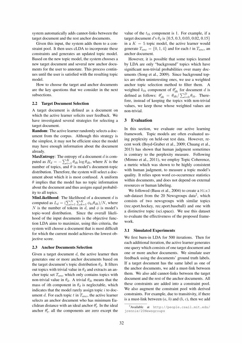
system automatically adds cannot-links between thetarget document and the rest anchor documents.
Given this input, the system adds them to a con-straint pool. It then uses cLDA to incorporate theseconstraints and generates an updated topic model.Based on the new topic model, the system chooses anew target document and several new anchor docu-ments for the user to annotate. This process contin-ues until the user is satisfied with the resulting topicmodel.
How to choose the target and anchor documentsare the key questions that we consider in the nextsubsections.
2.2 Target Document SelectionA target document is defined as a document onwhich the active learner solicits user feedback. Wehave investigated several strategies for selecting atarget document.Random: The active learner randomly selects a doc-ument from the corpus. Although this strategy isthe simplest, it may not be efficient since the modelmay have enough information about the documentalready.MaxEntropy: The entropy of a document d is com-puted as Hd = −∑K
i=1 θdk log θdk, where K is thenumber of topics, and θ is model’s document-topicdistribution. Therefore, the system will select a doc-ument about which it is most confused. A uniformθ implies that the model has no topic informationabout the document and thus assigns equal probabil-ity to all topics.MinLikelihood: The likelihood of a document d iscomputed as Ld = (
∑Ni=1
∑Kk=1 φkiθdk)/N , where
N is the number of tokens in d, and φ is model’stopic-word distribution. Since the overall likeli-hood of the input documents is the objective func-tion LDA aims to maximize, using this criteria, thesystem will choose a document that is most difficultfor which the current model achieves the lowest ob-jective score.
2.3 Anchor Documents SelectionGiven a target document d, the active learner thengenerates one or more anchor documents based onthe target document’s topic distribution θd. It filtersout topics with trivial value in θd and extracts an an-chor topic set Tanc which only contains topics withnon-trivial value in θd. A trivial θdi means that themass of ith component in θd is neglectable, whichindicates that the model rarely assign topic i to doc-ument d. For each topic t in Tanc, the active learnerselects an anchor document who has minimum Eu-clidean distance with an ideal anchor θ′t. In the idealanchor θ′t, all the components are zero except the
value of the tth component is 1. For example, if atarget document d’s θd is {0.5, 0.3, 0.03, 0.02, 0.15}in a K = 5 topic model, the active learner wouldgenerate Tanc = {0, 1, 4} and for each t in Tanc, ananchor document.
However, it is possible that some topics learnedby LDA are only “background” topics which havesignificant non-trivial probabilities over many doc-uments (Song et al., 2009). Since background top-ics are often uninteresting ones, we use a weightedanchor topic selection method to filter them. Aweighted kth component of θ′dk for document d isdefined as follows: θ′dk = θdk/
∑Di=0 θik. There-
fore, instead of keeping the topics with non-trivialvalues, we keep those whose weighted values arenon-trivial.
3 Evaluation
In this section, we evaluate our active learningframework. Topic models are often evaluated us-ing perplexity on held-out test data. However, re-cent work (Boyd-Graber et al., 2009; Chuang et al.,2013) has shown that human judgment sometimesis contrary to the perplexity measure. Following(Mimno et al., 2011), we employ Topic Coherence,a metric which was shown to be highly consistentwith human judgment, to measure a topic model’squality. It relies upon word co-occurrence statisticswithin documents, and does not depend on externalresources or human labeling.
We followed (Basu et al., 2004) to create a Mix3sub-dataset from the 20 Newsgroups data2, whichconsists of two newsgroups with similar topics(rec.sport.hockey, rec.sport.baseball) and one witha distinctive topic (sci.space). We use this datasetto evaluate the effectiveness of the proposed frame-work.
3.1 Simulated Experiments
We first burn-in LDA for 500 iterations. Then foreach additional iteration, the active learner generatesone query which consists of one target document andone or more anchor documents. We simulate userfeedback using the documents’ ground truth labels.If a target document has the same label as one ofthe anchor documents, we add a must-link betweenthem. We also add cannot-links between the targetdocument and the rest of the anchor documents. Allthese constraints are added into a constraint pool.We also augment the constraint pool with derivedconstraints. For example, due to transitivity, if thereis a must-link between (a, b) and (b, c), then we add
2Available at http://people.csail.mit.edu/jrennie/20Newsgroups
32
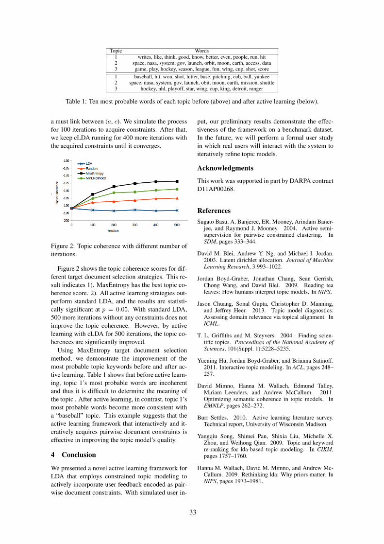
Topic Words1 writes, like, think, good, know, better, even, people, run, hit2 space, nasa, system, gov, launch, orbit, moon, earth, access, data3 game, play, hockey, season, league, fun, wing, cup, shot, score1 baseball, hit, won, shot, hitter, base, pitching, cub, ball, yankee2 space, nasa, system, gov, launch, obit, moon, earth, mission, shuttle3 hockey, nhl, playoff, star, wing, cup, king, detroit, ranger
Table 1: Ten most probable words of each topic before (above) and after active learning (below).
a must link between (a, c). We simulate the processfor 100 iterations to acquire constraints. After that,we keep cLDA running for 400 more iterations withthe acquired constraints until it converges.
Figure 2: Topic coherence with different number ofiterations.
Figure 2 shows the topic coherence scores for dif-ferent target document selection strategies. This re-sult indicates 1). MaxEntropy has the best topic co-herence score. 2). All active learning strategies out-perform standard LDA, and the results are statisti-cally significant at p = 0.05. With standard LDA,500 more iterations without any constraints does notimprove the topic coherence. However, by activelearning with cLDA for 500 iterations, the topic co-herences are significantly improved.
Using MaxEntropy target document selectionmethod, we demonstrate the improvement of themost probable topic keywords before and after ac-tive learning. Table 1 shows that before active learn-ing, topic 1’s most probable words are incoherentand thus it is difficult to determine the meaning ofthe topic . After active learning, in contrast, topic 1’smost probable words become more consistent witha “baseball” topic. This example suggests that theactive learning framework that interactively and it-eratively acquires pairwise document constraints iseffective in improving the topic model’s quality.
4 Conclusion
We presented a novel active learning framework forLDA that employs constrained topic modeling toactively incorporate user feedback encoded as pair-wise document constraints. With simulated user in-
put, our preliminary results demonstrate the effec-tiveness of the framework on a benchmark dataset.In the future, we will perform a formal user studyin which real users will interact with the system toiteratively refine topic models.
Acknowledgments
This work was supported in part by DARPA contractD11AP00268.
ReferencesSugato Basu, A. Banjeree, ER. Mooney, Arindam Baner-
jee, and Raymond J. Mooney. 2004. Active semi-supervision for pairwise constrained clustering. InSDM, pages 333–344.
David M. Blei, Andrew Y. Ng, and Michael I. Jordan.2003. Latent dirichlet allocation. Journal of MachineLearning Research, 3:993–1022.
Jordan Boyd-Graber, Jonathan Chang, Sean Gerrish,Chong Wang, and David Blei. 2009. Reading tealeaves: How humans interpret topic models. In NIPS.
Jason Chuang, Sonal Gupta, Christopher D. Manning,and Jeffrey Heer. 2013. Topic model diagnostics:Assessing domain relevance via topical alignment. InICML.
T. L. Griffiths and M. Steyvers. 2004. Finding scien-tific topics. Proceedings of the National Academy ofSciences, 101(Suppl. 1):5228–5235.
Yuening Hu, Jordan Boyd-Graber, and Brianna Satinoff.2011. Interactive topic modeling. In ACL, pages 248–257.
David Mimno, Hanna M. Wallach, Edmund Talley,Miriam Leenders, and Andrew McCallum. 2011.Optimizing semantic coherence in topic models. InEMNLP, pages 262–272.
Burr Settles. 2010. Active learning literature survey.Technical report, University of Wisconsin Madison.
Yangqiu Song, Shimei Pan, Shixia Liu, Michelle X.Zhou, and Weihong Qian. 2009. Topic and keywordre-ranking for lda-based topic modeling. In CIKM,pages 1757–1760.
Hanna M. Wallach, David M. Mimno, and Andrew Mc-Callum. 2009. Rethinking lda: Why priors matter. InNIPS, pages 1973–1981.
33
Proceedings of the Workshop on Interactive Language Learning, Visualization, and Interfaces, pages 34–37,Baltimore, Maryland, USA, June 27, 2014. c©2014 Association for Computational Linguistics
GLANCE Visualizes Lexical Phenomena for Language Learning
Mei-Hua Chen*, Shih-Ting Huang+, Ting-Hui Kao+, Sun-Wen Chiu+, Tzu-His Yen+ * Department of Foreign Languages and Literature, Hua Fan University, Taipei, Taiwan,
R.O.C. 22301 + Department of Computer Science, National Tsing Hua University, HsinChu, Taiwan,
R.O.C. 30013
{chen.meihua,koromiko1104,maxis1718,chiuhsunwen, joseph.yen}@gmail.com
Abstract
Facilitating vocabulary knowledge is a
challenging aspect for language learners.
Although current corpus-based reference
tools provide authentic contextual clues, the
plain text format is not conducive to fully
illustrating some lexical phenomena. Thus,
this paper proposes GLANCE1
, a text
visualization tool, to present a large amount
of lexical phenomena using charts and graphs,
aimed at helping language learners
understand a word quickly and intuitively. To
evaluate the effectiveness of the system, we
designed interfaces to allow comparison
between text and graphics presentation, and
conducted a preliminary user study with ESL
students. The results show that the visualized
display is of greater benefit to the
understanding of word characteristics than
textual display.
1 Introduction
Vocabulary is a challenging aspect for language
learners to master. Extended word knowledge,
such as word polarity and position, is not widely
available in traditional dictionaries. Thus, for
most language learners, it is very difficult to
have a good command of such lexical phenome-
na.
Current linguistics software programs use
large corpus data to advance language learning.
The use of corpora exposes learners to authentic
contextual clues and lets them discover patterns
or collocations of words from contextual clues
(Partington, 1998). However, a huge amount of
data can be overwhelming and time-consuming
(Yeh et al., 2007) for language learners to induce
rules or patterns. On the other hand, some lexical
phenomena seem unable to be comprehended
1 http://glance-it.herokuapp.com/
fast and directly in plain text format (Koo, 2006).
For example, in the British National Corpus
(2007), “however” seems more negative than
“but”. Also, compared with “but”, “however”
appears more frequently at the beginning of a
sentence.
With this in mind, we proposed GLANCE1, a
text visualization tool, which presents corpus
data using charts and graphs to help language
learners understand the lexical phenomena of a
word quickly and intuitively. In this paper, we
focused on five types of lexical phenomena: po-
larity, position, POS, form and discipline, which
will be detailed in the Section 3. Given a single
query word, the GLANCE system shows graph-
ical representations of its lexical phenomena se-
quentially within a single web page.
Additionally we believe that the use of
graphics also facilitates the understanding of the
differences between two words. Taking this into
consideration, we introduce a comparison mode
to help learners differentiate two words at a
glance. Allowing two word input, GLANCE
draws the individual representative graphs for
both words and presents these graphs in a two-
column view. The display of parallel graphs de-
picts the distinctions between the two words
clearly.
2 Related Work
Corpus-based language learning has widened the
perspectives in second and foreign language edu-
cation, such as vocabulary learning (Wood,
2001). In past decades, various corpus-based ref-
erence tools have been developed. For example,
WordSmith (Scott, 2000), Compleat Lexical Tu-
tor (Cobb, 2007), GRASP (Huang et al., 2011),
PREFER (Chen et al, 2012).
Recently, some interactive visualization tools
have been developed for the purpose of illustrat-
ing various linguistic phenomena. Three exam-
34
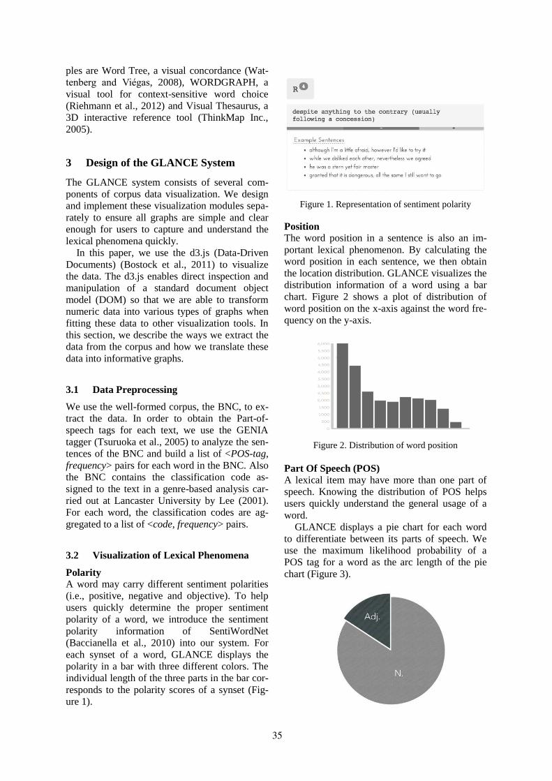
ples are Word Tree, a visual concordance (Wat-
tenberg and i gas, 2008), WORDGRAPH, a
visual tool for context-sensitive word choice
(Riehmann et al., 2012) and Visual Thesaurus, a
3D interactive reference tool (ThinkMap Inc.,
2005).
3 Design of the GLANCE System
The GLANCE system consists of several com-
ponents of corpus data visualization. We design
and implement these visualization modules sepa-
rately to ensure all graphs are simple and clear
enough for users to capture and understand the
lexical phenomena quickly.
In this paper, we use the d3.js (Data-Driven
Documents) (Bostock et al., 2011) to visualize
the data. The d3.js enables direct inspection and
manipulation of a standard document object
model (DOM) so that we are able to transform
numeric data into various types of graphs when
fitting these data to other visualization tools. In
this section, we describe the ways we extract the
data from the corpus and how we translate these
data into informative graphs.
3.1 Data Preprocessing
We use the well-formed corpus, the BNC, to ex-
tract the data. In order to obtain the Part-of-
speech tags for each text, we use the GENIA
tagger (Tsuruoka et al., 2005) to analyze the sen-
tences of the BNC and build a list of <POS-tag,
frequency> pairs for each word in the BNC. Also
the BNC contains the classification code as-
signed to the text in a genre-based analysis car-
ried out at Lancaster University by Lee (2001).
For each word, the classification codes are ag-
gregated to a list of <code, frequency> pairs.
3.2 Visualization of Lexical Phenomena
Polarity
A word may carry different sentiment polarities
(i.e., positive, negative and objective). To help
users quickly determine the proper sentiment
polarity of a word, we introduce the sentiment
polarity information of SentiWordNet
(Baccianella et al., 2010) into our system. For
each synset of a word, GLANCE displays the
polarity in a bar with three different colors. The
individual length of the three parts in the bar cor-
responds to the polarity scores of a synset (Fig-
ure 1).
Figure 1. Representation of sentiment polarity
Position
The word position in a sentence is also an im-
portant lexical phenomenon. By calculating the
word position in each sentence, we then obtain
the location distribution. GLANCE visualizes the
distribution information of a word using a bar
chart. Figure 2 shows a plot of distribution of
word position on the x-axis against the word fre-
quency on the y-axis.
Figure 2. Distribution of word position
Part Of Speech (POS)
A lexical item may have more than one part of
speech. Knowing the distribution of POS helps
users quickly understand the general usage of a
word.
GLANCE displays a pie chart for each word
to differentiate between its parts of speech. We
use the maximum likelihood probability of a
POS tag for a word as the arc length of the pie
chart (Figure 3).
35
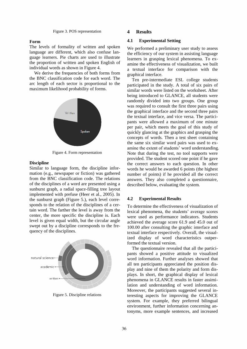
Figure 3. POS representation
Form
The levels of formality of written and spoken
language are different, which also confuse lan-
guage learners. Pie charts are used to illustrate
the proportion of written and spoken English of
individual words as shown in Figure 4.
We derive the frequencies of both forms from
the BNC classification code for each word. The
arc length of each sector is proportional to the
maximum likelihood probability of forms.
Figure 4. Form representation
Discipline
Similar to language form, the discipline infor-
mation (e.g., newspaper or fiction) was gathered
from the BNC classification code. The relations
of the disciplines of a word are presented using a
sunburst graph, a radial space-filling tree layout
implemented with prefuse (Heer et al., 2005). In
the sunburst graph (Figure 5.), each level corre-
sponds to the relation of the disciplines of a cer-
tain word. The farther the level is away from the
center, the more specific the discipline is. Each
level is given equal width, but the circular angle
swept out by a discipline corresponds to the fre-
quency of the disciplines.
Figure 5. Discipline relations
4 Results
4.1 Experimental Setting
We performed a preliminary user study to assess
the efficiency of our system in assisting language
learners in grasping lexical phenomena. To ex-
amine the effectiveness of visualization, we built
a textual interface for comparison with the
graphical interface.
Ten pre-intermediate ESL college students
participated in the study. A total of six pairs of
similar words were listed on the worksheet. After
being introduced to GLANCE, all students were
randomly divided into two groups. One group
was required to consult the first three pairs using
the graphical interface and the second three pairs
the textual interface, and vice versa. The partici-
pants were allowed a maximum of one minute
per pair, which meets the goal of this study of
quickly glancing at the graphics and grasping the
concepts of words. Then a test sheet containing
the same six similar word pairs was used to ex-
amine the extent of students’ word understanding.
Note that during the test, no tool supports were
provided. The student scored one point if he gave
the correct answers to each question. In other
words he would be awarded 6 points (the highest
number of points) if he provided all the correct
answers. They also completed a questionnaire,
described below, evaluating the system.
4.2 Experimental Results
To determine the effectiveness of visualization of
lexical phenomena, the students’ average scores
were used as performance indicators. Students
achieved the average score 61.9 and 45.0 out of
100.00 after consulting the graphic interface and
textual interface respectively. Overall, the visual-
ized display of word characteristics outper-
formed the textual version.
The questionnaire revealed that all the partici-
pants showed a positive attitude to visualized
word information. Further analyses showed that
all ten participants appreciated the position dis-
play and nine of them the polarity and form dis-
plays. In short, the graphical display of lexical
phenomena in GLANCE results in faster assimi-
lation and understanding of word information.
Moreover, the participants suggested several in-
teresting aspects for improving the GLANCE
system. For example, they preferred bilingual
environment, further information concerning an-
tonyms, more example sentences, and increased
36
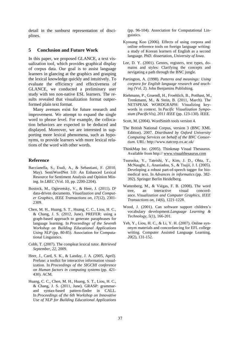
detail in the sunburst representation of disci-
plines.
5 Conclusion and Future Work
In this paper, we proposed GLANCE, a text vis-
ualization tool, which provides graphical display
of corpus data. Our goal is to assist language
learners in glancing at the graphics and grasping
the lexical knowledge quickly and intuitively. To
evaluate the efficiency and effectiveness of
GLANCE, we conducted a preliminary user
study with ten non-native ESL learners. The re-
sults revealed that visualization format outper-
formed plain text format.
Many avenues exist for future research and
improvement. We attempt to expand the single
word to phrase level. For example, the colloca-
tion behaviors are expected to be deduced and
displayed. Moreover, we are interested in sup-
porting more lexical phenomena, such as hypo-
nyms, to provide learners with more lexical rela-
tions of the word with other words.
Reference
Baccianella, S., Esuli, A., & Sebastiani, F. (2010,
May). SentiWordNet 3.0: An Enhanced Lexical
Resource for Sentiment Analysis and Opinion Min-
ing. In LREC (Vol. 10, pp. 2200-2204).
Bostock, M., Ogievetsky, V., & Heer, J. (2011). D³
data-driven documents. Visualization and Comput-
er Graphics, IEEE Transactions on, 17(12), 2301-
2309.
Chen, M. H., Huang, S. T., Huang, C. C., Liou, H. C.,
& Chang, J. S. (2012, June). PREFER: using a
graph-based approach to generate paraphrases for
language learning. In Proceedings of the Seventh
Workshop on Building Educational Applications
Using NLP (pp. 80-85). Association for Computa-
tional Linguistics.
Cobb, T. (2007). The compleat lexical tutor. Retrieved
September, 22, 2009.
Heer, J., Card, S. K., & Landay, J. A. (2005, April).
Prefuse: a toolkit for interactive information visual-
ization. In Proceedings of the SIGCHI conference
on Human factors in computing systems (pp. 421-
430). ACM.
Huang, C. C., Chen, M. H., Huang, S. T., Liou, H. C.,
& Chang, J. S. (2011, June). GRASP: grammar-
and syntax-based pattern-finder in CALL.
In Proceedings of the 6th Workshop on Innovative
Use of NLP for Building Educational Applications
(pp. 96-104). Association for Computational Lin-
guistics.
Kyosung Koo (2006). Effects of using corpora and
online reference tools on foreign language writing:
a study of Korean learners of English as a second
language. PhD. dissertation, University of Iowa.
Lee, D. Y. (2001). Genres, registers, text types, do-
mains and styles: Clarifying the concepts and
nevigating a path through the BNC jungle.
Partington, A. (1998). Patterns and meanings: Using
corpora for English language research and teach-
ing (Vol. 2). John Benjamins Publishing.
Riehmann, P., Gruendl, H., Froehlich, B., Potthast, M.,
Trenkmann, M., & Stein, B. (2011, March). The
NETSPEAK WORDGRAPH: Visualizing key-
words in context. In Pacific Visualization Sympo-
sium (PacificVis), 2011 IEEE (pp. 123-130). IEEE.
Scott, M. (2004). WordSmith tools version 4.
The British National Corpus, version 3 (BNC XML
Edition). 2007. Distributed by Oxford University
Computing Services on behalf of the BNC Consor-
tium. URL: http://www.natcorp.ox.ac.uk/
ThinkMap Inc. (2005). Thinkmap Visual Thesaurus.
Available from http:// www.visualthesaurus.com
Tsuruoka, Y., Tateishi, Y., Kim, J. D., Ohta, T.,
McNaught, J., Ananiadou, S., & Tsujii, J. I. (2005).
Developing a robust part-of-speech tagger for bio-
medical text. In Advances in informatics (pp. 382-
392). Springer Berlin Heidelberg.
Wattenberg, M., & Viégas, F. B. (2008). The word
tree, an interactive visual concord-
ance. Visualization and Computer Graphics, IEEE
Transactions on, 14(6), 1221-1228.
Wood, J. (2001). Can software support children’s
vocabulary development.Language Learning &
Technology, 5(1), 166-201.
Yeh, Y., Liou, H. C., & Li, Y. H. (2007). Online syn-
onym materials and concordancing for EFL college
writing. Computer Assisted Language Learning,
20(2), 131-152.
37
Proceedings of the Workshop on Interactive Language Learning, Visualization, and Interfaces, pages 38–44,Baltimore, Maryland, USA, June 27, 2014. c©2014 Association for Computational Linguistics
SPIED: Stanford Pattern-based Information Extraction and Diagnostics
Sonal Gupta Christopher D. ManningDepartment of Computer Science
Stanford University{sonal, manning}@cs.stanford.edu
Abstract
This paper aims to provide an effectiveinterface for progressive refinement ofpattern-based information extraction sys-tems. Pattern-based information extrac-tion (IE) systems have an advantage overmachine learning based systems that pat-terns are easy to customize to cope witherrors and are interpretable by humans.Building a pattern-based system is usuallyan iterative process of trying different pa-rameters and thresholds to learn patternsand entities with high precision and recall.Since patterns are interpretable to humans,it is possible to identify sources of errors,such as patterns responsible for extract-ing incorrect entities and vice-versa, andcorrect them. However, it involves timeconsuming manual inspection of the ex-tracted output. We present a light-weighttool, SPIED, to aid IE system develop-ers in learning entities using patterns withbootstrapping, and visualizing the learnedentities and patterns with explanations.SPIED is the first publicly available tool tovisualize diagnostic information of multi-ple pattern learning systems to the best ofour knowledge.
1 Introduction
Entity extraction using rules dominates commer-cial industry, mainly because rules are effective,interpretable by humans, and easy to customize tocope with errors (Chiticariu et al., 2013). Rules,which can be hand crafted or learned by a sys-tem, are commonly created by looking at the con-text around already known entities, such as surfaceword patterns (Hearst, 1992) and dependency pat-terns (Yangarber et al., 2000). Building a pattern-based learning system is usually a repetitive pro-cess, usually performed by the system developer,
of manually examining a system’s output to iden-tify improvements or errors introduced by chang-ing the entity or pattern extractor. Interpretabil-ity of patterns makes it easier for humans to iden-tify sources of errors by inspecting patterns thatextracted incorrect instances or instances that re-sulted in learning of bad patterns. Parametersrange from window size of the context in surfaceword patterns to thresholds for learning a candi-date entity. At present, there is a lack of toolshelping a system developer to understand resultsand to improve results iteratively.
Visualizing diagnostic information of a systemand contrasting it with another system can makethe iterative process easier and more efficient. Forexample, consider a user trying to decide on thecontext’s window size in surface words patterns.And the user deliberates that part-of-speech (POS)restriction of context words might be required fora reduced window size to avoid extracting erro-neous mentions.1 By comparing and contrastingextractions of two systems with different parame-ters, the user can investigate the cases in which thePOS restriction is required with smaller windowsize, and whether the restriction causes the systemto miss some correct entities. In contrast, compar-ing just accuracy of two systems does not allowinspecting finer details of extractions that increaseor decrease accuracy and to make changes accord-ingly.
In this paper, we present a pattern-based entitylearning and diagnostics tool, SPIED. It consistsof two components: 1. pattern-based entity learn-ing using bootstrapping (SPIED-Learn), and 2. vi-sualizing the output of one or two entity learningsystems (SPIED-Viz). SPIED-Viz is independentof SPIED-Learn and can be used with any pattern-based entity learner. For demonstration, we usethe output of SPIED-Learn as an input to SPIED-
1A shorter context size usually extracts entities withhigher recall but lower precision.
38
Viz. SPIED-Viz has pattern-centric and entity-centric views, which visualize learned patternsand entities, respectively, and the explanations forlearning them. SPIED-Viz can also contrast twosystems by comparing the ranks of learned enti-ties and patterns. In this paper, as a concrete ex-ample, we learn and visualize drug-treatment (DT)entities from unlabeled patient-generated medicaltext, starting with seed dictionaries of entities formultiple classes. The task was proposed and fur-ther developed in Gupta and Manning (2014b)and Gupta and Manning (2014a).
Our contributions in this paper are: 1. wepresent a novel diagnostic tool for visual-ization of output of multiple pattern-basedentity learning systems, and 2. we release thecode of an end-to-end pattern learning sys-tem, which learns entities using patterns in abootstrapped system and visualizes its diag-nostic output. The pattern learning code isavailable at http://nlp.stanford.edu/software/patternslearning.shtml.The visualization code is available athttp://nlp.stanford.edu/software/patternviz.shtml.
2 Learning Patterns and Entities
Bootstrapped systems have been commonly usedto learn entities (Riloff, 1996; Collins and Singer,1999). SPIED-Learn is based on the system de-scribed in Gupta and Manning (2014a), whichbuilds upon the previous bootstrapped pattern-learning work and proposed an improved mea-sure to score patterns (Step 3 below). It learnsentities for given classes from unlabeled text bybootstrapping from seed dictionaries. Patternsare learned using labeled entities, and entities arelearned based on the extractions of learned pat-terns. The process is iteratively performed untilno more patterns or entities can be learned. Thefollowing steps give a short summary of the itera-tive learning of entities belonging to a class DT:
1. Data labeling: The text is labeled using theclass dictionaries, starting with the seed dic-tionaries in the first iteration. A phrasematching a dictionary phrase is labeled withthe dictionary’s class.
2. Pattern generation: Patterns are generated us-ing the context around the positively labeledentities to create candidate patterns for DT.
3. Pattern learning: Candidate patterns arescored using a pattern scoring measure andthe top ones are added to the list of learnedpatterns for DT. The maximum number ofpatterns learned is given as an input to thesystem by the developer.
4. Entity learning: Learned patterns for the classare applied to the text to extract candidate en-tities. An entity scorer ranks the candidateentities and adds the top entities to DT’s dic-tionary. The maximum number of entitieslearned is given as an input to the system bythe developer.
5. Repeat steps 1-4 for a given number of itera-tions.
SPIED provides an option to use any of the pat-tern scoring measures described in (Riloff, 1996;Thelen and Riloff, 2002; Yangarber et al., 2002;Lin et al., 2003; Gupta and Manning, 2014b). Apattern is scored based on the positive, negative,and unlabeled entities it extracts. The positive andnegative labels of entities are heuristically deter-mined by the system using the dictionaries and theiterative entity learning process. The oracle labelsof learned entities are not available to the learningsystem. Note that an entity that the system consid-ered positive might actually be incorrect, since theseed dictionaries can be noisy and the system canlearn incorrect entities in the previous iterations,and vice-versa. SPIED’s entity scorer is the sameas in Gupta and Manning (2014a).
Each candidate entity is scored using weights ofthe patterns that extract it and other entity scoringmeasures, such as TF-IDF. Thus, learning of eachentity can be explained by the learned patterns thatextract it, and learning of each pattern can be ex-plained by all the entities it extracts.
3 Visualizing Diagnostic Information
SPIED-Viz visualizes learned entities and patternsfrom one or two entity learning systems, and thediagnostic information associated with them. Itoptionally uses the oracle labels of learned enti-ties to color code them, and contrast their ranksof correct/incorrect entities when comparing twosystems. The oracle labels are usually determinedby manually judging each learned entity as cor-rect or incorrect. SPIED-Viz has two views: 1. apattern-centric view that visualizes patterns of one
39
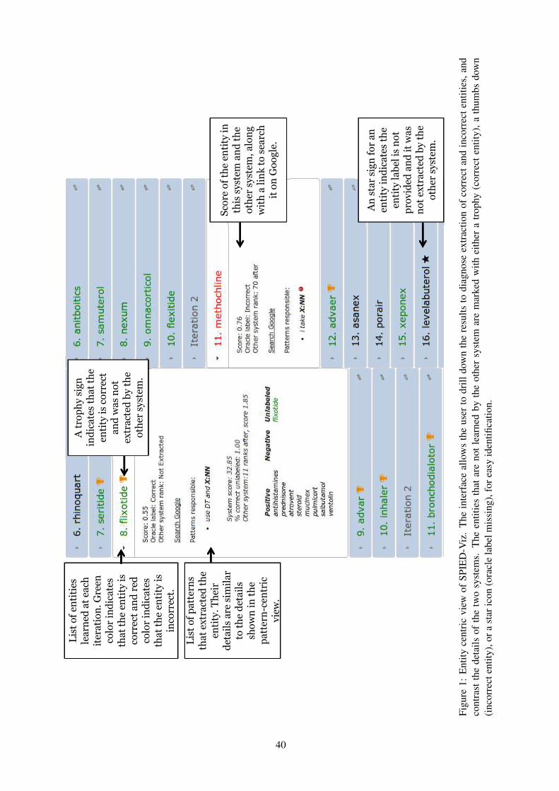
Sco
re o
f th
e en
tity
in
th
is s
yst
em a
nd
th
e o
ther
sy
stem
, a
lon
g
wit
h a
lin
k t
o s
earc
h
it o
n G
oo
gle
.
An
sta
r si
gn
fo
r a
n
enti
ty i
nd
ica
tes
the
enti
ty l
ab
el i
s n
ot
pro
vid
ed a
nd
it
wa
s n
ot
extr
act
ed b
y t
he
oth
er s
yst
em.
A t
rop
hy
sig
n
ind
ica
tes
tha
t th
e en
tity
is
corr
ect
an
d w
as
no
t ex
tra
cted
by
th
e o
ther
sy
stem
.
Lis
t o
f en
titi
es
lea
rned
at
each
it
era
tio
n.
Gre
en
colo
r in
dic
ate
s th
at
the
enti
ty i
s co
rrec
t a
nd
red
co
lor
ind
ica
tes
tha
t th
e en
tity
is
inco
rrec
t.
Lis
t o
f p
att
ern
s th
at
extr
act
ed t
he
enti
ty.
Th
eir
det
ail
s a
re s
imil
ar
to t
he
det
ail
s sh
ow
n i
n t
he
pa
tter
n-c
entr
ic
vie
w.
Figu
re1:
Ent
ityce
ntri
cvi
ewof
SPIE
D-V
iz.
The
inte
rfac
eal
low
sth
eus
erto
drill
dow
nth
ere
sults
todi
agno
seex
trac
tion
ofco
rrec
tand
inco
rrec
tent
ities
,and
cont
rast
the
deta
ilsof
the
two
syst
ems.
The
entit
ies
that
are
notl
earn
edby
the
othe
rsy
stem
are
mar
ked
with
eith
era
trop
hy(c
orre
cten
tity)
,ath
umbs
dow
n(i
ncor
rect
entit
y),o
rast
aric
on(o
racl
ela
belm
issi
ng),
fore
asy
iden
tifica
tion.
40
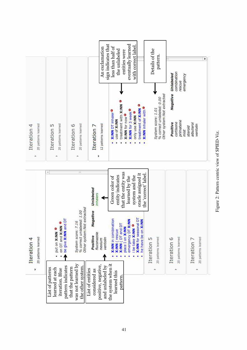
Lis
t o
f en
titi
es
con
sid
ered
as
po
siti
ve,
neg
ati
ve,
a
nd
un
lab
eled
by
th
e sy
stem
wh
en i
t le
arn
ed t
his
p
att
ern
.
An
ex
cla
ma
tio
n
sig
n i
nd
ica
tes
tha
t le
ss t
ha
n h
alf
of
the
un
lab
eled
en
titi
es w
ere
even
tua
lly
lea
rned
w
ith
co
rrec
t la
bel
.
Det
ail
s o
f th
e p
att
ern
.
Gre
en c
olo
r o
f en
tity
in
dic
ate
s th
at
the
enti
ty w
as
lea
rned
by
th
e sy
stem
an
d t
he
ora
cle
ass
ign
ed i
t th
e ‘c
orr
ect’
la
bel
.
Lis
t o
f p
att
ern
s le
arn
ed a
t ea
ch
iter
ati
on
. B
lue
pa
tter
n i
nd
ica
tes
tha
t th
e p
att
ern
w
as
no
t le
arn
ed b
y
the
oth
er s
yst
em.
Figu
re2:
Patte
rnce
ntri
cvi
ewof
SPIE
D-V
iz.
41
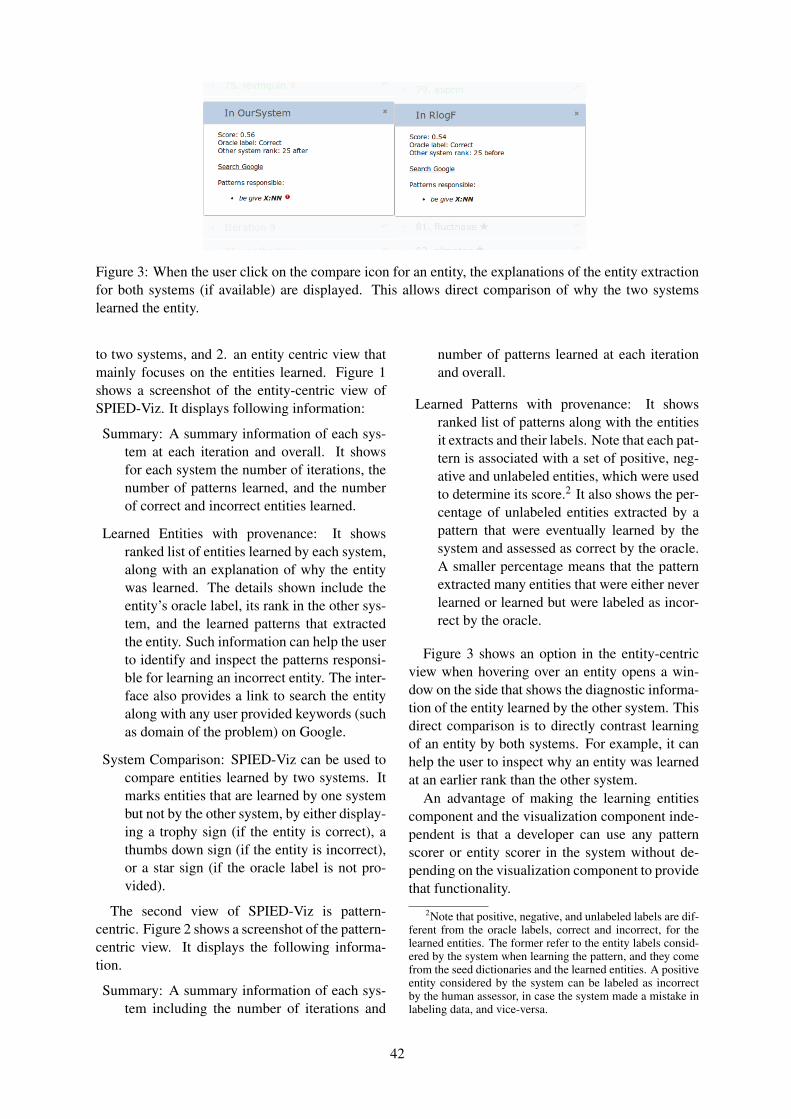
Figure 3: When the user click on the compare icon for an entity, the explanations of the entity extractionfor both systems (if available) are displayed. This allows direct comparison of why the two systemslearned the entity.
to two systems, and 2. an entity centric view thatmainly focuses on the entities learned. Figure 1shows a screenshot of the entity-centric view ofSPIED-Viz. It displays following information:
Summary: A summary information of each sys-tem at each iteration and overall. It showsfor each system the number of iterations, thenumber of patterns learned, and the numberof correct and incorrect entities learned.
Learned Entities with provenance: It showsranked list of entities learned by each system,along with an explanation of why the entitywas learned. The details shown include theentity’s oracle label, its rank in the other sys-tem, and the learned patterns that extractedthe entity. Such information can help the userto identify and inspect the patterns responsi-ble for learning an incorrect entity. The inter-face also provides a link to search the entityalong with any user provided keywords (suchas domain of the problem) on Google.
System Comparison: SPIED-Viz can be used tocompare entities learned by two systems. Itmarks entities that are learned by one systembut not by the other system, by either display-ing a trophy sign (if the entity is correct), athumbs down sign (if the entity is incorrect),or a star sign (if the oracle label is not pro-vided).
The second view of SPIED-Viz is pattern-centric. Figure 2 shows a screenshot of the pattern-centric view. It displays the following informa-tion.
Summary: A summary information of each sys-tem including the number of iterations and
number of patterns learned at each iterationand overall.
Learned Patterns with provenance: It showsranked list of patterns along with the entitiesit extracts and their labels. Note that each pat-tern is associated with a set of positive, neg-ative and unlabeled entities, which were usedto determine its score.2 It also shows the per-centage of unlabeled entities extracted by apattern that were eventually learned by thesystem and assessed as correct by the oracle.A smaller percentage means that the patternextracted many entities that were either neverlearned or learned but were labeled as incor-rect by the oracle.
Figure 3 shows an option in the entity-centricview when hovering over an entity opens a win-dow on the side that shows the diagnostic informa-tion of the entity learned by the other system. Thisdirect comparison is to directly contrast learningof an entity by both systems. For example, it canhelp the user to inspect why an entity was learnedat an earlier rank than the other system.
An advantage of making the learning entitiescomponent and the visualization component inde-pendent is that a developer can use any patternscorer or entity scorer in the system without de-pending on the visualization component to providethat functionality.
2Note that positive, negative, and unlabeled labels are dif-ferent from the oracle labels, correct and incorrect, for thelearned entities. The former refer to the entity labels consid-ered by the system when learning the pattern, and they comefrom the seed dictionaries and the learned entities. A positiveentity considered by the system can be labeled as incorrectby the human assessor, in case the system made a mistake inlabeling data, and vice-versa.
42
4 System Details
SPIED-Learn uses TokensRegex (Chang andManning, 2014) to create and apply surface wordpatterns to text. SPIED-Viz takes details oflearned entities and patterns as input in a JSONformat. It uses Javascript, angular, and jquery tovisualize the information in a web browser.
5 Related Work
Most interactive IE systems focus on annotationof text, labeling of entities, and manual writingof rules. Some annotation and labeling tools are:MITRE’s Callisto3, Knowtator4, SAPIENT (Li-akata et al., 2009), brat5, Melita (Ciravegna et al.,2002), and XConc Suite (Kim et al., 2008). Akbiket al. (2013) interactively helps non-expert usersto manually write patterns over dependency trees.GATE6 provides the JAPE language that recog-nizes regular expressions over annotations. Othersystems focus on reducing manual effort for de-veloping extractors (Brauer et al., 2011; Li et al.,2011). In contrast, our tool focuses on visualizingand comparing diagnostic information associatedwith pattern learning systems.
WizIE (Li et al., 2012) is an integrated environ-ment for annotating text and writing pattern ex-tractors for information extraction. It also gener-ates regular expressions around labeled mentionsand suggests patterns to users. It is most similarto our tool as it displays an explanation of the re-sults extracted by a pattern. However, it is focusedtowards hand writing and selection of rules. In ad-dition, it cannot be used to directly compare twopattern learning systems.
What’s Wrong With My NLP?7 is a tool forjointly visualizing various natural language pro-cessing formats such as trees, graphs, and entities.It can be used alongside our system to visualizethe patterns since we mainly focus on diagnosticinformation.
6 Future Work and Conclusion
We plan to add a feature for a user to providethe oracle label of a learned entity using the in-terface. Currently, the oracle labels are assignedoffline. We also plan to extend SPIED to visualize
3http://callisto.mitre.org4http://knowtator.sourceforge.net5http://brat.nlplab.org6http://gate.ac.uk7https://code.google.com/p/whatswrong
diagnostic information of learned relations from apattern-based relation learning system. Anotheravenue of future work is to evaluate SPIED-Vizby studying its users and their interactions withthe system. In addition, we plan to improve thevisualization by summarizing the diagnostic infor-mation, such as which parameters led to what mis-takes, to make it easier to understand for systemsthat extract large number of patterns and entities.
In conclusion, we present a novel diagnostictool for pattern-based entity learning that visual-izes and compares output of one to two systems.It is light-weight web browser based visualization.The visualization can be used with any pattern-based entity learner. We make the code of an end-to-end system freely available for research pur-pose. The system learns entities and patterns usingbootstrapping starting with seed dictionaries, andvisualizes the diagnostic output. We hope SPIEDwill help other researchers and users to diagnoseerrors and tune parameters in their pattern-basedentity learning system in an easy and efficient way.
ReferencesAlan Akbik, Oresti Konomi, and Michail Melnikov.
2013. Propminer: A workflow for interactive infor-mation extraction and exploration using dependencytrees. In ACL (Conference System Demonstrations),pages 157–162.
Falk Brauer, Robert Rieger, Adrian Mocan, and Woj-ciech M. Barczynski. 2011. Enabling informationextraction by inference of regular expressions fromsample entities. In CIKM, pages 1285–1294.
Angel X. Chang and Christopher D. Manning. 2014.TokensRegex: Defining cascaded regular expres-sions over tokens. In Stanford University TechnicalReport.
Laura Chiticariu, Yunyao Li, and Frederick R. Reiss.2013. Rule-based information extraction is dead!long live rule-based information extraction systems!In Proceedings of the Conference on EmpiricalMethods in Natural Language Processing, EMNLP’13, pages 827–832.
Fabio Ciravegna, Alexiei Dingli, Daniela Petrelli, andYorick Wilks. 2002. User-system cooperationin document annotation based on information ex-traction. In In Proceedings of the 13th Interna-tional Conference on Knowledge Engineering andKnowledge Management, EKAW02, pages 122–137.Springer Verlag.
Michael Collins and Yoram Singer. 1999. Unsuper-vised models for named entity classification. In Pro-ceedings of the Joint SIGDAT Conference on Empir-
43
ical Methods in Natural Language Processing andVery Large Corpora, pages 100–110.
Sonal Gupta and Christopher D. Manning. 2014a. Im-proved pattern learning for bootstrapped entity ex-traction. In Proceedings of the Eighteenth Confer-ence on Computational Natural Language Learning(CoNLL).
Sonal Gupta and Christopher D. Manning. 2014b. In-duced lexico-syntactic patterns improve informationextraction from online medical forums. Under Sub-mission.
Marti A Hearst. 1992. Automatic acquisition of hy-ponyms from large text corpora. In Proceedings ofthe 14th International Conference on Computationallinguistics, COLING ’92, pages 539–545.
Jin-Dong Kim, Tomoko Ohta, and Jun ichi Tsujii.2008. Corpus annotation for mining biomedicalevents from literature. BMC Bioinformatics.
Yunyao Li, Vivian Chu, Sebastian Blohm, HuaiyuZhu, and Howard Ho. 2011. Facilitating pat-tern discovery for relation extraction with semantic-signature-based clustering. In Proceedings of the20th ACM International Conference on Informa-tion and Knowledge Management, CIKM ’11, pages1415–1424.
Yunyao Li, Laura Chiticariu, Huahai Yang, Freder-ick R. Reiss, and Arnaldo Carreno-fuentes. 2012.Wizie: A best practices guided development envi-ronment for information extraction. In Proceedingsof the ACL 2012 System Demonstrations, ACL ’12,pages 109–114.
Maria Liakata, Claire Q, and Larisa N. Soldatova.2009. Semantic annotation of papers: Interface &enrichment tool (sapient). In Proceedings of theBioNLP 2009 Workshop, pages 193–200.
Winston Lin, Roman Yangarber, and Ralph Grishman.2003. Bootstrapped learning of semantic classesfrom positive and negative examples. In Proceed-ings of the ICML 2003 Workshop on The Continuumfrom Labeled to Unlabeled Data in Machine Learn-ing and Data Mining.
Ellen Riloff. 1996. Automatically generating extrac-tion patterns from untagged text. In Proceedingsof the 13th National Conference on Artificial Intelli-gence, AAAI’96, pages 1044–1049.
Michael Thelen and Ellen Riloff. 2002. A bootstrap-ping method for learning semantic lexicons usingextraction pattern contexts. In Proceedings of theConference on Empirical Methods in Natural Lan-guage Processing, EMNLP ’02, pages 214–221.
Roman Yangarber, Ralph Grishman, and PasiTapanainen. 2000. Automatic acquisition ofdomain knowledge for information extraction. InProceedings of the 18th International Conferenceon Computational Linguistics, COLING ’00, pages940–946.
Roman Yangarber, Winston Lin, and Ralph Grishman.2002. Unsupervised learning of generalized names.In Proceedings of the 19th International Conferenceon Computational Linguistics, COLING ’02.
44
Proceedings of the Workshop on Interactive Language Learning, Visualization, and Interfaces, pages 45–52,Baltimore, Maryland, USA, June 27, 2014. c©2014 Association for Computational Linguistics
Interactive Exploration of Asynchronous Conversations: Applying aUser-centered Approach to Design a Visual Text Analytic System
Enamul Hoque, Giuseppe Carenini{enamul,carenini}@cs.ubc.ca
Department of Computer ScienceUniversity of British Columbia
Vancouver, Canada
Shafiq [email protected]
Qatar Computing Research InstituteQatar Foundation
Doha, Qatar
Abstract
Exploring an online conversation can bevery difficult for a user, especially whenit becomes a long complex thread. We fol-low a human-centered design approach totightly integrate text mining methods withinteractive visualization techniques to sup-port the users in fulfilling their informa-tion needs. The resulting visual text ana-lytic system provides multifaceted explo-ration of asynchronous conversations. Wediscuss a number of open challenges andpossible directions for further improve-ment including the integration of interac-tive human feedback in the text miningloop, applying more advanced text analy-sis methods with visualization techniques,and evaluating the system with real users.
1 Introduction
With the rapid adoption of Web-based social me-dia, asynchronous online conversations are be-coming extremely common for supporting com-munication and collaboration. An asynchronousconversation such as a blog may start with a newsarticle or an editorial opinion, and later generate along and complex thread as comments are addedby the participants (Carenini et al., 2011). Con-sider a scenario, where a reader opens a blog con-versation about Obama’s healthcare policy. Thereader wants to know why people are supportingor opposing ObamaCare. However, since somerelated discussion topics like student loan and jobrecession are introduced, the reader finds it hardto keep track of the comments about ObamaCare,which end up being buried in the long discussion.This may lead to an information overload problem,where the reader gets overwhelmed, starts to skipcomments, and eventually leaves the conversationwithout satisfying her information needs (Jones etal., 2004).
How can we support the user in performing thisand similar information seeking tasks? Arguably,supporting this task requires tight integration be-tween Natural Language Processing (NLP) and in-formation visualization (InfoVis) techniques, butwhat specific text analysis methods should be ap-plied? What metadata of the conversation could beuseful to the user? How this data should be visual-ized to the user? And even more importantly, howNLP and InfoVis techniques should be effectivelyintegrated? Our hypothesis is that to answer thesequestions effectively, we need to apply human-centered design methodologies originally devisedfor generic InfoVis (e.g., (Munzner, 2009; Sedl-mair et al., 2012)). Starting from an analysis ofuser behaviours and needs in the target conversa-tional domain, such methods help uncover usefultask and data abstractions that can guide systemdesign. On the one hand, task and data abstrac-tions can characterize the type of information thatneeds to be extracted from the conversation; on theother hand, they can inform the design of the vi-sual encodings and interaction techniques. Moretellingly, as both the NLP and the InfoVis compo-nents of the resulting system refer to a common setof task and data abstractions, they are more likelyto be consistent and synergistic.
We have explored this hypothesis in developingConVis, a visual analytic system to support the in-teractive analysis of blog conversations. In the firstpart of the paper, we describe the development ofConVis, from characterizing the domain of blogs,its users, tasks and data, to designing and imple-menting specific NLP and InfoVis techniques in-formed by our user-centered design. In the secondpart of the paper, starting from an informal evalu-ation of Convis and a comprehensive literature re-view, we discuss several ideas on how ConVis (andsimilar systems) could be further improved andtested. These include the integration of interac-tive human feedback in the text mining techniques
45
(which are based on Machine Learning), the cou-pling of even more advanced NLP methods withthe InfoVis techniques, and the challenges in run-ning evaluations of ConVis and similar interfaces.
2 Related Work
While in the last decade, NLP and InfoVis meth-ods have been investigated to support the user inmaking sense of conversational data, most of thiswork has been limited in several ways.
For example, earlier works on visualizingasynchronous conversations primarily investigatedhow to reveal the thread structure of a conversationusing tree visualization techniques, such as usinga mixed-model visualization to show both chrono-logical sequence and reply relationships (Venoliaand Neustaedter, 2003), thumbnail metaphor usinga sequence of rectangles (Wattenberg and Millen,2003; Kerr, 2003), and radial tree layout (Pascual-Cid and Kaltenbrunner, 2009). However, such vi-sualizations did not focus on analysing the actualcontent (i.e., the text) of the conversations, whichis something that according to our user-centred de-sign users are very interested in.
On the other hand, text mining approachesthat perform content analysis of the conversations,such as finding primary themes (or topics) withinconversations (Sack, 2000; Dave et al., 2004), orvisualizing the content evolution over time (Wei etal., 2010; Viegas et al., 2006), often did not derivetheir visual encodings and interactive techniquesfrom task and data abstractions based on a detailedanalysis of specific user needs and requirements inthe target domains.
Furthermore, more on the technical side, thetext analysis methods employed by these ap-proaches are not designed to exploit the spe-cific characteristics of asynchronous conversations(e.g., use of quotation). Recently, (Joty et al.,2013b) has shown that topic segmentation and la-beling models are more accurate when these spe-cific characteristics are taken into account. Themethods presented in (Joty et al., 2013b) areadopted in ConVis.
In general, to the best of our knowledge, noprevious work has applied user-centred design totightly integrate text mining methods with interac-tive visualization in the domain of asynchronousconversations.
3 Domains and User Activities
Conversational domains: The phenomenal adop-tion of novel Web-based social media has lead tothe rise of textual conversations in many differentmodalities. While email remains a fundamentalway of communicating for most people, other con-versational modalities such as blogs, microblogs(e.g., Twitter) and discussion fora have quickly be-come widely popular. Since the nature of data andtasks may vary significantly from one domain tothe other, rather than trying to build an one-size-fit-all interface, we follow a design methodologythat is driven by modeling the tasks and usagecharacteristics in a specific domain.
In this work, we focus on blogs, where peoplecan express their thoughts and engage in onlinediscussions. Due to the large number of commentswith complex thread structure (Joty et al., 2013b),mining and visualizing blog conversations can be-come a challenging problem. However, the visual-ization can be effective for other threaded discus-sions (e.g., news stories, Youtube comments).
Users: As shown in Table 1, blog users can becategorized into two groups based on their activ-ities: (a) participants who already contributed tothe conversations, and (b) non-participants whowish to join the conversations or analyze the con-versations. Depending on different user groups thetasks might vary as well, something that needs tobe taken into account in the design process.
For example, imagine a participant who has ex-pressed her opinion about a major political issue.After some time, she may become interested toknow what comments were made supporting oropposing her opinion, and whether those com-ments require a reply right away. On the contrary,a non-participant, who is interested in joining theongoing conversation on that particular politicalissue, may want to decide whether and how sheshould contribute by quickly skimming through along thread of blog comments. Another group ofusers may include the analysts, a policy maker forinstance, who does not wish to join the conversa-tion, but may want to make an informed decisionbased on a summary of arguments used to supportor oppose the political issue.
Once the conversation becomes inactive (i.e.,no further comments are added), still a distinctionmay remain between the activities of participantsand non-participants on tasks (see Table 1). In ourwork, we have initially concentrated on supporting
46
Usertypes
Ongoing conver-sation
Inactive/past conver-sation
Participant Already joined theconversation (wantsto get updated andpossibly make newcomments)
Wants to delve intothe past conversationsand re-examine whatwas discussed, whatshe commented on,what other peoplereplied, etc.
Non-participant
Potential partici-pant (wants to jointhe conversation)Analyst (wants toanalyze the ongo-ing conversation,but does not intendto join)
Wants to analyze andgain insight about thepast conversation.
Table 1: User categorization for asynchronousconversation.
the non-participant’s activity on an inactive con-versation (as opposed to an ongoing conversation).
4 Designing ConVis: From Tasks to NLPand InfoVis Techniques
We now briefly describe our design approach forintegrating text mining techniques with interactivevisualization in ConVis. We first characterize thedomain of blogs and perform the data and tasksabstraction according to the nested model of de-sign study (Munzner, 2009). We then mine thedata as appeared to be essential from that data andtask analysis, followed by iteratively refining thedesign of ConVis that aims to effectively supportthe identified blog reading tasks (A more detailedanalysis of the task abstractions and visual designis provided in (Hoque and Carenini, 2014)).
4.1 TasksTo understand the blog reading tasks, we re-viewed the literature focusing on why and howpeople read blogs. From the analysis, wefound that the primary goals of reading blogs in-clude information seeking, fact checking, guid-ance/opinion seeking, and political surveillance(Kaye, 2005). People may also read blogs to con-nect to their communities of interest (Dave et al.,2004; Mishne, 2006), or just for fun/ enjoyment(Baumer et al., 2008; Kaye, 2005).
Some studies have also revealed interesting be-havioural patterns of blog readers. For example,people often look for variety of opinions and havetendencies to switch from one topic to anotherquickly (Singh et al., 2010; Munson and Resnick,
2010). In addition, they often exhibit exploratorybehaviour, i.e., they quickly skim through a fewposts about a topic before delving deeper into itsdetails (Zinman, 2011). Therefore, the interfaceshould facilitate open-ended exploration, by pro-viding navigational cues that help the user to seekinteresting comments.
From the analyses of primary goals of blogreading, we compile a list of tasks and the asso-ciated data variables that one would wish to visu-alize for these tasks. These tasks can be framedas a set of questions, for instance, ‘what do peo-ple say about topic X?’, ‘how other people’s view-points differ from my current viewpoint on topicX?’, ‘what are some interesting/funny commentsto read?’ We then identify the primary data vari-ables involved in these tasks and their abstracttypes. For instance, most of these questions in-volve topics discussed and sentiments expressedin the conversation. Note that some questions mayadditionally require to know people-centric infor-mation and relate such information to the visual-ization design. We also identify a set of meta-data to be useful cues for navigating a conversa-tion (the position of the comments, thread struc-ture, and comment length) (Narayan and Cheshire,2010; Baumer et al., 2008). We choose to encodethe position of the comments (ordinal) as opposedto their timestamps (quantitative); since the exacttimestamp of a comment is less important to usersthan its chronological position with respect to theother comments (Baumer et al., 2008).
4.2 Text Analysis
Since most of the blog reading tasks we identi-fied involved topics and sentiments expressed inthe conversation, we applied both topic modelingand sentiment analysis on a given conversation.
In topic modeling, we group the sentences of ablog conversation into a number of topical clustersand label each cluster by assigning a short infor-mative topic descriptor (i.e., a keyphrase). To findthe topical clusters and their associated labels, weapply the topic segmentation and labeling modelsrecently proposed by (Joty et al., 2013b) for asyn-chronous conversations, and successfully evalu-ated on email and blog datasets. More specifically,for topic segmentation, we use their best unsu-pervised topic segmentation model LCSeg+FQG,which extends the generic lexical cohesion basedtopic segmenter (LCSeg) (Galley et al., 2003)
47
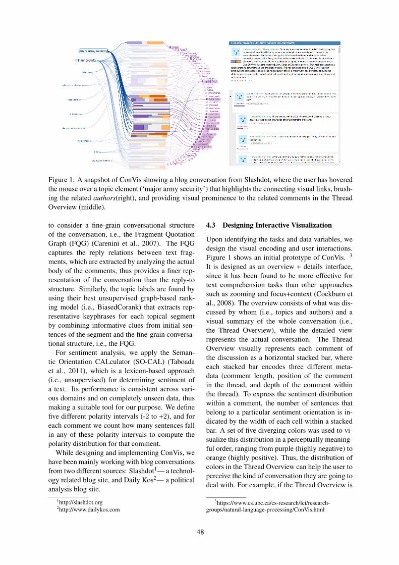
Figure 1: A snapshot of ConVis showing a blog conversation from Slashdot, where the user has hoveredthe mouse over a topic element (‘major army security’) that highlights the connecting visual links, brush-ing the related authors(right), and providing visual prominence to the related comments in the ThreadOverview (middle).
to consider a fine-grain conversational structureof the conversation, i.e., the Fragment QuotationGraph (FQG) (Carenini et al., 2007). The FQGcaptures the reply relations between text frag-ments, which are extracted by analyzing the actualbody of the comments, thus provides a finer rep-resentation of the conversation than the reply-tostructure. Similarly, the topic labels are found byusing their best unsupervised graph-based rank-ing model (i.e., BiasedCorank) that extracts rep-resentative keyphrases for each topical segmentby combining informative clues from initial sen-tences of the segment and the fine-grain conversa-tional structure, i.e., the FQG.
For sentiment analysis, we apply the Seman-tic Orientation CALculator (SO-CAL) (Taboadaet al., 2011), which is a lexicon-based approach(i.e., unsupervised) for determining sentiment ofa text. Its performance is consistent across vari-ous domains and on completely unseen data, thusmaking a suitable tool for our purpose. We definefive different polarity intervals (-2 to +2), and foreach comment we count how many sentences fallin any of these polarity intervals to compute thepolarity distribution for that comment.
While designing and implementing ConVis, wehave been mainly working with blog conversationsfrom two different sources: Slashdot1— a technol-ogy related blog site, and Daily Kos2— a politicalanalysis blog site.
1http://slashdot.org2http://www.dailykos.com
4.3 Designing Interactive Visualization
Upon identifying the tasks and data variables, wedesign the visual encoding and user interactions.Figure 1 shows an initial prototype of ConVis. 3
It is designed as an overview + details interface,since it has been found to be more effective fortext comprehension tasks than other approachessuch as zooming and focus+context (Cockburn etal., 2008). The overview consists of what was dis-cussed by whom (i.e., topics and authors) and avisual summary of the whole conversation (i.e.,the Thread Overview), while the detailed viewrepresents the actual conversation. The ThreadOverview visually represents each comment ofthe discussion as a horizontal stacked bar, whereeach stacked bar encodes three different meta-data (comment length, position of the commentin the thread, and depth of the comment withinthe thread). To express the sentiment distributionwithin a comment, the number of sentences thatbelong to a particular sentiment orientation is in-dicated by the width of each cell within a stackedbar. A set of five diverging colors was used to vi-sualize this distribution in a perceptually meaning-ful order, ranging from purple (highly negative) toorange (highly positive). Thus, the distribution ofcolors in the Thread Overview can help the user toperceive the kind of conversation they are going todeal with. For example, if the Thread Overview is
3https://www.cs.ubc.ca/cs-research/lci/research-groups/natural-language-processing/ConVis.html
48
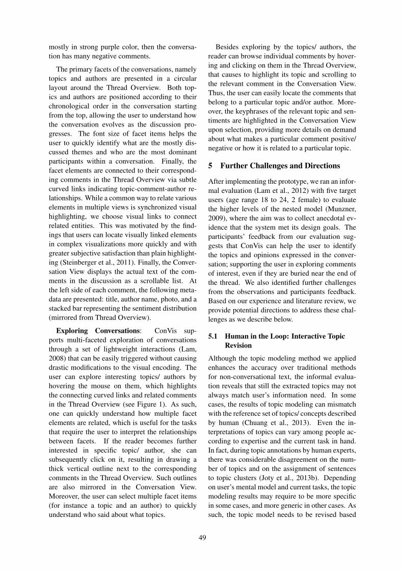
mostly in strong purple color, then the conversa-tion has many negative comments.
The primary facets of the conversations, namelytopics and authors are presented in a circularlayout around the Thread Overview. Both top-ics and authors are positioned according to theirchronological order in the conversation startingfrom the top, allowing the user to understand howthe conversation evolves as the discussion pro-gresses. The font size of facet items helps theuser to quickly identify what are the mostly dis-cussed themes and who are the most dominantparticipants within a conversation. Finally, thefacet elements are connected to their correspond-ing comments in the Thread Overview via subtlecurved links indicating topic-comment-author re-lationships. While a common way to relate variouselements in multiple views is synchronized visualhighlighting, we choose visual links to connectrelated entities. This was motivated by the find-ings that users can locate visually linked elementsin complex visualizations more quickly and withgreater subjective satisfaction than plain highlight-ing (Steinberger et al., 2011). Finally, the Conver-sation View displays the actual text of the com-ments in the discussion as a scrollable list. Atthe left side of each comment, the following meta-data are presented: title, author name, photo, and astacked bar representing the sentiment distribution(mirrored from Thread Overview).
Exploring Conversations: ConVis sup-ports multi-faceted exploration of conversationsthrough a set of lightweight interactions (Lam,2008) that can be easily triggered without causingdrastic modifications to the visual encoding. Theuser can explore interesting topics/ authors byhovering the mouse on them, which highlightsthe connecting curved links and related commentsin the Thread Overview (see Figure 1). As such,one can quickly understand how multiple facetelements are related, which is useful for the tasksthat require the user to interpret the relationshipsbetween facets. If the reader becomes furtherinterested in specific topic/ author, she cansubsequently click on it, resulting in drawing athick vertical outline next to the correspondingcomments in the Thread Overview. Such outlinesare also mirrored in the Conversation View.Moreover, the user can select multiple facet items(for instance a topic and an author) to quicklyunderstand who said about what topics.
Besides exploring by the topics/ authors, thereader can browse individual comments by hover-ing and clicking on them in the Thread Overview,that causes to highlight its topic and scrolling tothe relevant comment in the Conversation View.Thus, the user can easily locate the comments thatbelong to a particular topic and/or author. More-over, the keyphrases of the relevant topic and sen-timents are highlighted in the Conversation Viewupon selection, providing more details on demandabout what makes a particular comment positive/negative or how it is related to a particular topic.
5 Further Challenges and Directions
After implementing the prototype, we ran an infor-mal evaluation (Lam et al., 2012) with five targetusers (age range 18 to 24, 2 female) to evaluatethe higher levels of the nested model (Munzner,2009), where the aim was to collect anecdotal ev-idence that the system met its design goals. Theparticipants’ feedback from our evaluation sug-gests that ConVis can help the user to identifythe topics and opinions expressed in the conver-sation; supporting the user in exploring commentsof interest, even if they are buried near the end ofthe thread. We also identified further challengesfrom the observations and participants feedback.Based on our experience and literature review, weprovide potential directions to address these chal-lenges as we describe below.
5.1 Human in the Loop: Interactive TopicRevision
Although the topic modeling method we appliedenhances the accuracy over traditional methodsfor non-conversational text, the informal evalua-tion reveals that still the extracted topics may notalways match user’s information need. In somecases, the results of topic modeling can mismatchwith the reference set of topics/ concepts describedby human (Chuang et al., 2013). Even the in-terpretations of topics can vary among people ac-cording to expertise and the current task in hand.In fact, during topic annotations by human experts,there was considerable disagreement on the num-ber of topics and on the assignment of sentencesto topic clusters (Joty et al., 2013b). Dependingon user’s mental model and current tasks, the topicmodeling results may require to be more specificin some cases, and more generic in other cases. Assuch, the topic model needs to be revised based
49
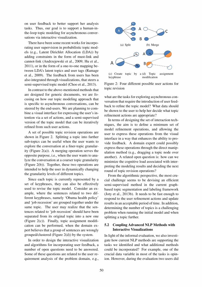
on user feedback to better support her analysistasks. Thus, our goal is to support a human-in-the-loop topic modeling for asynchronous conver-sations via interactive visualization.
There have been some recent works for incorpo-rating user supervision in probabilistic topic mod-els (e.g., Latent Dirichlet Allocation (LDA)) byadding constraints in the form of must-link andcannot-link (Andrzejewski et al., 2009; Hu et al.,2011), or in the form of a one-to-one mapping be-tween LDA’s latent topics and user tags (Ramageet al., 2009). The feedback from users has beenalso integrated through visualizations, that steers asemi-supervised topic model (Choo et al., 2013).
In contrast to the above-mentioned methods thatare designed for generic documents, we are fo-cusing on how our topic modeling approach thatis specific to asynchronous conversations, can besteered by the end-users. We are planning to com-bine a visual interface for expressing the user’s in-tention via a set of actions, and a semi-supervisedversion of the topic model that can be iterativelyrefined from such user actions.
A set of possible topic revision operations areshown in Figure 2. Splitting a topic into furthersub-topics can be useful when the user wants toexplore the conversation at a finer-topic granular-ity (Figure 2(a)). A merging operation serves theopposite purpose, i.e., when the user wants to ana-lyze the conversation at a coarser topic granularity(Figure 2(b)). Together, these two operations areintended to help the user in dynamically changingthe granularity levels of different topics.
Since each topic is currently represented by aset of keyphrases, they can also be effectivelyused to revise the topic model. Consider an ex-ample, where the sentences related to two dif-ferent keyphrases, namely ‘Obama health policy’and ‘job recession’ are grouped together under thesame topic. The user may realize that the sen-tences related to ‘job recession’ should have beenseparated from its original topic into a new one(Figure 2(c)). Finally, topic assignment modifi-cation can be performed, when the domain ex-pert believes that a group of sentences are wronglygrouped/clustered (Figure 2(d)) by the system.
In order to design the interactive visualizationand algorithms for incorporating user feedback, anumber of open questions need to be answered.Some of these questions are related to the user re-quirement analysis of the problem domain, e.g.,
(a) Split (b) Merge
(c) Create topic by akeyphrase
(d) Topic assignmentmodification
Figure 2: Four different possible user actions fortopic revision
what are the tasks for exploring asynchronous con-versation that require the introduction of user feed-back to refine the topic model? What data shouldbe shown to the user to help her decide what topicrefinement actions are appropriate?
In terms of designing the set of interaction tech-niques, the aim is to define a minimum set ofmodel refinement operations, and allowing theuser to express these operations from the visualinterface in a way that enhances the ability to pro-vide feedback. A domain expert could possiblyexpress these operations through the direct manip-ulation method (e.g., dragging a topic node overanother). A related open question is: how can weminimize the cognitive load associated with inter-preting the modeling results and deciding the nextround of topic revision operations?
From the algorithmic perspective, the most cru-cial challenge seems to be devising an efficientsemi-supervised method in the current graph-based topic segmentation and labeling framework(Joty et al., 2013b). It needs to be fast enough torespond to the user refinement actions and updateresults in an acceptable period of time. In addition,determining the number of topics is a challengingproblem when running the initial model and whensplitting a topic further.
5.2 Coupling Advanced NLP Methods withInteractive Visualizations
In light of the informal evaluation, we also investi-gate how current NLP methods are supporting thetasks we identified and what additional methodscould be incorporated? For example, one of thecrucial data variable in most of the tasks is opin-ion. However, during the evaluation two users did
50
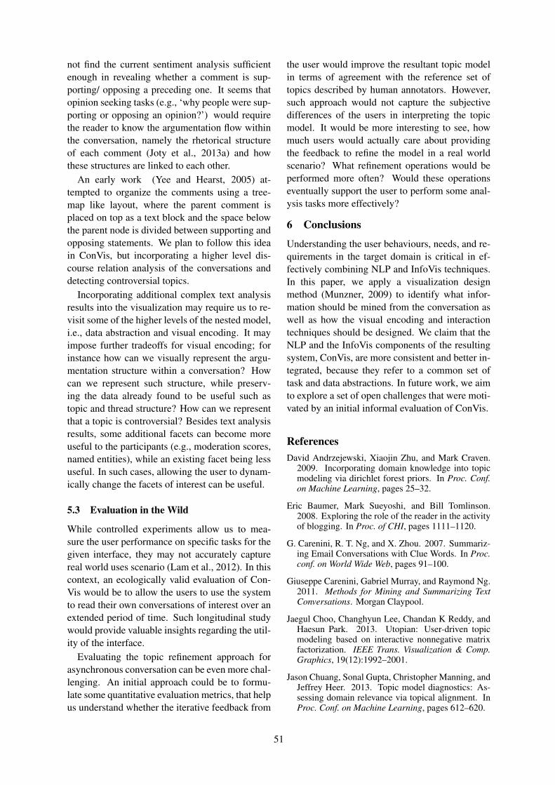
not find the current sentiment analysis sufficientenough in revealing whether a comment is sup-porting/ opposing a preceding one. It seems thatopinion seeking tasks (e.g., ‘why people were sup-porting or opposing an opinion?’) would requirethe reader to know the argumentation flow withinthe conversation, namely the rhetorical structureof each comment (Joty et al., 2013a) and howthese structures are linked to each other.
An early work (Yee and Hearst, 2005) at-tempted to organize the comments using a tree-map like layout, where the parent comment isplaced on top as a text block and the space belowthe parent node is divided between supporting andopposing statements. We plan to follow this ideain ConVis, but incorporating a higher level dis-course relation analysis of the conversations anddetecting controversial topics.
Incorporating additional complex text analysisresults into the visualization may require us to re-visit some of the higher levels of the nested model,i.e., data abstraction and visual encoding. It mayimpose further tradeoffs for visual encoding; forinstance how can we visually represent the argu-mentation structure within a conversation? Howcan we represent such structure, while preserv-ing the data already found to be useful such astopic and thread structure? How can we representthat a topic is controversial? Besides text analysisresults, some additional facets can become moreuseful to the participants (e.g., moderation scores,named entities), while an existing facet being lessuseful. In such cases, allowing the user to dynam-ically change the facets of interest can be useful.
5.3 Evaluation in the Wild
While controlled experiments allow us to mea-sure the user performance on specific tasks for thegiven interface, they may not accurately capturereal world uses scenario (Lam et al., 2012). In thiscontext, an ecologically valid evaluation of Con-Vis would be to allow the users to use the systemto read their own conversations of interest over anextended period of time. Such longitudinal studywould provide valuable insights regarding the util-ity of the interface.
Evaluating the topic refinement approach forasynchronous conversation can be even more chal-lenging. An initial approach could be to formu-late some quantitative evaluation metrics, that helpus understand whether the iterative feedback from
the user would improve the resultant topic modelin terms of agreement with the reference set oftopics described by human annotators. However,such approach would not capture the subjectivedifferences of the users in interpreting the topicmodel. It would be more interesting to see, howmuch users would actually care about providingthe feedback to refine the model in a real worldscenario? What refinement operations would beperformed more often? Would these operationseventually support the user to perform some anal-ysis tasks more effectively?
6 Conclusions
Understanding the user behaviours, needs, and re-quirements in the target domain is critical in ef-fectively combining NLP and InfoVis techniques.In this paper, we apply a visualization designmethod (Munzner, 2009) to identify what infor-mation should be mined from the conversation aswell as how the visual encoding and interactiontechniques should be designed. We claim that theNLP and the InfoVis components of the resultingsystem, ConVis, are more consistent and better in-tegrated, because they refer to a common set oftask and data abstractions. In future work, we aimto explore a set of open challenges that were moti-vated by an initial informal evaluation of ConVis.
ReferencesDavid Andrzejewski, Xiaojin Zhu, and Mark Craven.
2009. Incorporating domain knowledge into topicmodeling via dirichlet forest priors. In Proc. Conf.on Machine Learning, pages 25–32.
Eric Baumer, Mark Sueyoshi, and Bill Tomlinson.2008. Exploring the role of the reader in the activityof blogging. In Proc. of CHI, pages 1111–1120.
G. Carenini, R. T. Ng, and X. Zhou. 2007. Summariz-ing Email Conversations with Clue Words. In Proc.conf. on World Wide Web, pages 91–100.
Giuseppe Carenini, Gabriel Murray, and Raymond Ng.2011. Methods for Mining and Summarizing TextConversations. Morgan Claypool.
Jaegul Choo, Changhyun Lee, Chandan K Reddy, andHaesun Park. 2013. Utopian: User-driven topicmodeling based on interactive nonnegative matrixfactorization. IEEE Trans. Visualization & Comp.Graphics, 19(12):1992–2001.
Jason Chuang, Sonal Gupta, Christopher Manning, andJeffrey Heer. 2013. Topic model diagnostics: As-sessing domain relevance via topical alignment. InProc. Conf. on Machine Learning, pages 612–620.
51
Andy Cockburn, Amy Karlson, and Benjamin B Bed-erson. 2008. A review of overview+ detail, zoom-ing, and focus+ context interfaces. ACM ComputingSurveys (CSUR), 41(1):2.
Kushal Dave, Martin Wattenberg, and Michael Muller.2004. Flash forums and forumreader: navigating anew kind of large-scale online discussion. In Proc.ACM Conf. on CSCW, pages 232–241.
Michel Galley, Kathleen McKeown, Eric Fosler-Lussier, and Hongyan Jing. 2003. Discourse seg-mentation of multi-party conversation. In Proc. ofACL, pages 562–569.
Enamul Hoque and Giuseppe Carenini. 2014. ConVis:A visual text analytic system for exploring blog con-versations. (Computer Graphic Forum (to appear)).
Yuening Hu, Jordan Boyd-Graber, and Brianna Sati-noff. 2011. Interactive topic modeling. In Proc. ofACL.
Quentin Jones, Gilad Ravid, and Sheizaf Rafaeli. 2004.Information overload and the message dynamicsof online interaction spaces: A theoretical modeland empirical exploration. Information Systems Re-search, 15(2):194–210.
Shafiq Joty, Giuseppe Carenini, Raymond Ng, andYashar Mehdad. 2013a. Combining intra-andmulti-sentential rhetorical parsing for document-level discourse analysis. In Proc. of ACL.
Shafiq Joty, Giuseppe Carenini, and Raymond T Ng.2013b. Topic segmentation and labeling in asyn-chronous conversations. Journal of Artificial Intelli-gence Research, 47:521–573.
B. K. Kaye. 2005. Web side story: An exploratorystudy of why weblog users say they use weblogs.AEJMC Annual Conf.
Bernard Kerr. 2003. Thread arcs: An email threadvisualization. In IEEE Symposium on InformationVisualization, pages 211–218.
H. Lam, E. Bertini, P. Isenberg, C. Plaisant, andS. Carpendale. 2012. Empirical studies in infor-mation visualization: Seven scenarios. IEEE Trans.Visualization & Comp. Graphics, 18(9):1520–1536.
Heidi Lam. 2008. A framework of interaction costsin information visualization. IEEE Trans. Visualiza-tion & Comp. Graphics, 14(6):1149–1156.
Gilad Mishne. 2006. Information access challenges inthe blogspace. In Workshop on Intelligent Informa-tion Access (IIIA).
Sean A Munson and Paul Resnick. 2010. Presentingdiverse political opinions: how and how much. InProc. of CHI, pages 1457–1466.
Tamara Munzner. 2009. A nested model for visualiza-tion design and validation. IEEE Trans. Visualiza-tion & Comp. Graphics, 15(6):921–928.
S. Narayan and C. Cheshire. 2010. Not too long toread: The tldr interface for exploring and navigatinglarge-scale discussion spaces. In Hawaii Conf. onSystem Sciences (HICSS), pages 1–10.
Vıctor Pascual-Cid and Andreas Kaltenbrunner. 2009.Exploring asynchronous online discussions throughhierarchical visualisation. In IEEE Conf. on Infor-mation Visualization, pages 191–196.
Daniel Ramage, David Hall, Ramesh Nallapati, andChristopher D Manning. 2009. Labeled LDA: A su-pervised topic model for credit attribution in multi-labeled corpora. In Proc. of EMNLP, pages 248–256.
Warren Sack. 2000. Conversation map: an interfacefor very-large-scale conversations. Journal of Man-agement Information Systems, 17(3):73–92.
Michael Sedlmair, Miriah Meyer, and Tamara Mun-zner. 2012. Design study methodology: reflectionsfrom the trenches and the stacks. IEEE Trans. Visu-alization & Comp. Graphics, 18(12):2431–2440.
Param Vir Singh, Nachiketa Sahoo, and TridasMukhopadhyay. 2010. Seeking variety: A dynamicmodel of employee blog reading behavior. Availableat SSRN 1617405.
Markus Steinberger, Manuela Waldner, Marc Streit,Alexander Lex, and Dieter Schmalstieg. 2011.Context-preserving visual links. IEEE Trans. Visu-alization & Comp. Graphics, 17(12):2249–2258.
Maite Taboada, Julian Brooke, Milan Tofiloski, Kim-berly Voll, and Manfred Stede. 2011. Lexicon-based methods for sentiment analysis. Computa-tional linguistics, 37(2):267–307.
Gina Danielle Venolia and Carman Neustaedter. 2003.Understanding sequence and reply relationshipswithin email conversations: a mixed-model visual-ization. In Proc. of CHI, pages 361–368.
Fernanda B Viegas, Scott Golder, and Judith Donath.2006. Visualizing email content: portraying rela-tionships from conversational histories. In Proc. ofCHI, pages 979–988.
Martin Wattenberg and David Millen. 2003. Conver-sation thumbnails for large-scale discussions. In ex-tended abstracts on CHI, pages 742–743.
Furu Wei, Shixia Liu, Yangqiu Song, Shimei Pan,Michelle X Zhou, Weihong Qian, Lei Shi, Li Tan,and Qiang Zhang. 2010. Tiara: a visual exploratorytext analytic system. In Proc. ACM Conf. on Knowl-edge Discovery and Data Mining, pages 153–162.
Ka-Ping Yee and Marti Hearst. 2005. Content-centered discussion mapping. Online Deliberation2005/DIAC-2005.
Aaron Robert Zinman. 2011. Me, myself, and my hy-perego: understanding people through the aggrega-tion of their digital footprints. Ph.D. thesis, MIT.
52
Proceedings of the Workshop on Interactive Language Learning, Visualization, and Interfaces, pages 53–58,Baltimore, Maryland, USA, June 27, 2014. c©2014 Association for Computational Linguistics
MUCK: A toolkit for extracting and visualizing semantic dimensions oflarge text collections
Rebecca WeissStanford UniversityStanford, CA, 94305
Abstract
Users with large text collections are of-ten faced with one of two problems; ei-ther they wish to retrieve a semantically-relevant subset of data from the collectionfor further scrutiny (needle-in-a-haystack)or they wish to glean a high-level un-derstanding of how a subset compares tothe parent corpus in the context of afore-mentioned semantic dimensions (forest-for-the-trees). In this paper, I describeMUCK1, an open-source toolkit that ad-dresses both of these problems through adistributed text processing engine with aninteractive visualization interface.
1 Introduction
As gathering large text collections grows increas-ingly feasible for non-technical users, individu-als such as journalists, marketing/communicationsanalysts, and social scientists are accumulatingvast quantities of documents in order to addresskey strategy or research questions. But thesegroups often lack the technical skills to work withlarge text collections, in that the conventional ap-proaches they employ (content analysis and indi-vidual document scrutiny) are not suitable for thescale of the data they have gathered. Thus, usersrequire tools with the capability to filter out irrel-evant documents while drilling-down to the docu-ments that they are most interested in investigatingwith closer scrutiny. Furthermore, they require thecapability to then evaluate their subset in context,as the contrast in attributes between their subsetand the full corpora can often address many rele-vant questions.
This paper introduces a work-in-progress: thedevelopment of a toolkit that aids non-technical
1Mechanical Understanding of Contextual Knowledge
users of large text collections by combining se-mantic search and semantic visualization methods.The purpose of this toolkit is two-fold: first, toease the technical burden of working with large-scale text collections by leveraging semantic infor-mation for the purposes of filtering a large collec-tion of text down to the select sample documentsthat matter most to the user; second, to allow theuser to visually explore semantic attributes of theirsubset in comparison to the rest of the text collec-tion.
Thus, this toolkit comprises two components:
1. a distributed text processing engine that de-creases the cost of annotating massive quan-tities of text data for natural language infor-mation
2. an interactive visualization interface that en-ables exploration of the collection along se-mantic dimensions, which then affords sub-sequent document selection and subset-to-corpora comparison
The text processing engine is extensible, en-abling the future development of plug-ins to al-low for tasks beyond the included natural languageprocessing tasks, such that future users can em-bed any sentence- or document-level task to theirprocessing pipeline. The visualization interface isbuilt upon search engine technologies to decreasesearch result latency to user requests, enabling ahigh level of interactivity.
2 Related work
The common theme of existing semantic searchand semantic visualization methods is to enablethe user to gain greater, meaningful insight into thestructure of their document collections through theuse of transparent, trustworthy methods (Chuanget al., 2012; Ramage et al., 2009). The desired in-sight can change depending on the intended task.
53
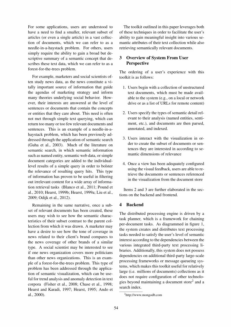
For some applications, users are understood tohave a need to find a smaller, relevant subset ofarticles (or even a single article) in a vast collec-tion of documents, which we can refer to as aneedle-in-a-haystack problem. For others, userssimply require the ability to gain a broad but de-scriptive summary of a semantic concept that de-scribes these text data, which we can refer to as aforest-for-the-trees problem.
For example, marketers and social scientists of-ten study news data, as the news constitute a vi-tally important source of information that guidethe agendas of marketing strategy and informmany theories underlying social behavior. How-ever, their interests are answered at the level ofsentences or documents that contain the conceptsor entities that they care about. This need is oftennot met through simple text querying, which canreturn too many or too few relevant documents andsentences. This is an example of a needle-in-a-haystack problem, which has been previously ad-dressed through the application of semantic search(Guha et al., 2003). Much of the literature onsemantic search, in which semantic informationsuch as named entity, semantic web data, or simpledocument categories are added to the individual-level results of a simple query in order to bolsterthe relevance of resulting query hits. This typeof information has proven to be useful in filteringout irrelevant content for a wide array of informa-tion retrieval tasks (Blanco et al., 2011; Pound etal., 2010; Hearst, 1999b; Hearst, 1999a; Liu et al.,2009; Odijk et al., 2012).
Remaining in the same narrative, once a sub-set of relevant documents has been created, theseusers may wish to see how the semantic charac-teristics of their subset contrast to the parent col-lection from which it was drawn. A marketer mayhave a desire to see how the tone of coverage innews related to their client’s brand compares tothe news coverage of other brands of a similartype. A social scientist may be interested to seeif one news organization covers more politiciansthan other news organizations. This is an exam-ple of a forest-for-the-trees problem. This type ofproblem has been addressed through the applica-tion of semantic visualization, which can be use-ful for trend analysis and anomaly detection in textcorpora (Fisher et al., 2008; Chase et al., 1998;Hearst and Karadi, 1997; Hearst, 1995; Ando etal., 2000).
The toolkit outlined in this paper leverages bothof these techniques in order to facilitate the user’sability to gain meaningful insight into various se-mantic attributes of their text collection while alsoretrieving semantically relevant documents.
3 Overview of System From UserPerspective
The ordering of a user’s experience with thistoolkit is as follows:
1. Users begin with a collection of unstructuredtext documents, which must be made avail-able to the system (e.g., on a local or networkdrive or as a list of URLs for remote content)
2. Users specify the types of semantic detail rel-evant to their analysis (named entities, senti-ment, etc.), and documents are then parsed,annotated, and indexed.
3. Users interact with the visualization in or-der to create the subset of documents or sen-tences they are interested in according to se-mantic dimensions of relevance
4. Once a view has been adequately configuredusing the visual feedback, users are able to re-trieve the documents or sentences referencedin the visualization from the document store
Items 2 and 3 are further elaborated in the sec-tions on the backend and frontend.
4 Backend
The distributed processing engine is driven by atask planner, which is a framework for chainingper-document tasks. As diagrammed in figure 1,the system creates and distributes text processingtasks needed to satisfy the user’s level of semanticinterest according to the dependencies between thevarious integrated third-party text processing li-braries. Additionally, this system does not possessdependencies on additional third-party large-scaleprocessing frameworks or message queueing sys-tems, which makes this toolkit useful for relativelylarge (i.e. millions of documents) collections as itdoes not require configuration of other technolo-gies beyond maintaining a document store2 and asearch index.
2http://www.mongodb.com
54
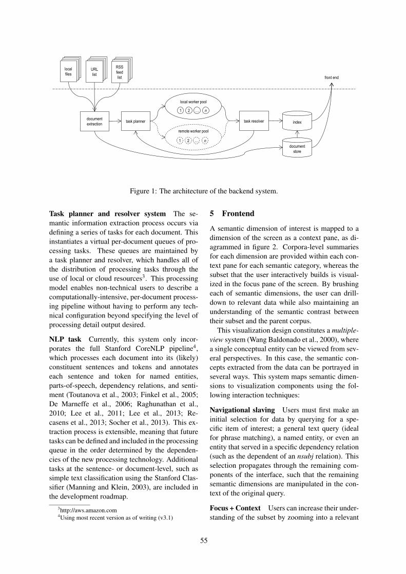
index task planner
local
files URL
list
RSS
feed
list
document
extraction
local worker pool
1 n 2 …
remote worker pool
1 n 2 …
document
store
front end
task resolver
Figure 1: The architecture of the backend system.
Task planner and resolver system The se-mantic information extraction process occurs viadefining a series of tasks for each document. Thisinstantiates a virtual per-document queues of pro-cessing tasks. These queues are maintained bya task planner and resolver, which handles all ofthe distribution of processing tasks through theuse of local or cloud resources3. This processingmodel enables non-technical users to describe acomputationally-intensive, per-document process-ing pipeline without having to perform any tech-nical configuration beyond specifying the level ofprocessing detail output desired.
NLP task Currently, this system only incor-porates the full Stanford CoreNLP pipeline4,which processes each document into its (likely)constituent sentences and tokens and annotateseach sentence and token for named entities,parts-of-speech, dependency relations, and senti-ment (Toutanova et al., 2003; Finkel et al., 2005;De Marneffe et al., 2006; Raghunathan et al.,2010; Lee et al., 2011; Lee et al., 2013; Re-casens et al., 2013; Socher et al., 2013). This ex-traction process is extensible, meaning that futuretasks can be defined and included in the processingqueue in the order determined by the dependen-cies of the new processing technology. Additionaltasks at the sentence- or document-level, such assimple text classification using the Stanford Clas-sifier (Manning and Klein, 2003), are included inthe development roadmap.
3http://aws.amazon.com4Using most recent version as of writing (v3.1)
5 Frontend
A semantic dimension of interest is mapped to adimension of the screen as a context pane, as di-agrammed in figure 2. Corpora-level summariesfor each dimension are provided within each con-text pane for each semantic category, whereas thesubset that the user interactively builds is visual-ized in the focus pane of the screen. By brushingeach of semantic dimensions, the user can drill-down to relevant data while also maintaining anunderstanding of the semantic contrast betweentheir subset and the parent corpus.
This visualization design constitutes a multiple-view system (Wang Baldonado et al., 2000), wherea single conceptual entity can be viewed from sev-eral perspectives. In this case, the semantic con-cepts extracted from the data can be portrayed inseveral ways. This system maps semantic dimen-sions to visualization components using the fol-lowing interaction techniques:
Navigational slaving Users must first make aninitial selection for data by querying for a spe-cific item of interest; a general text query (idealfor phrase matching), a named entity, or even anentity that served in a specific dependency relation(such as the dependent of an nsubj relation). Thisselection propagates through the remaining com-ponents of the interface, such that the remainingsemantic dimensions are manipulated in the con-text of the original query.
Focus + Context Users can increase their under-standing of the subset by zooming into a relevant
55
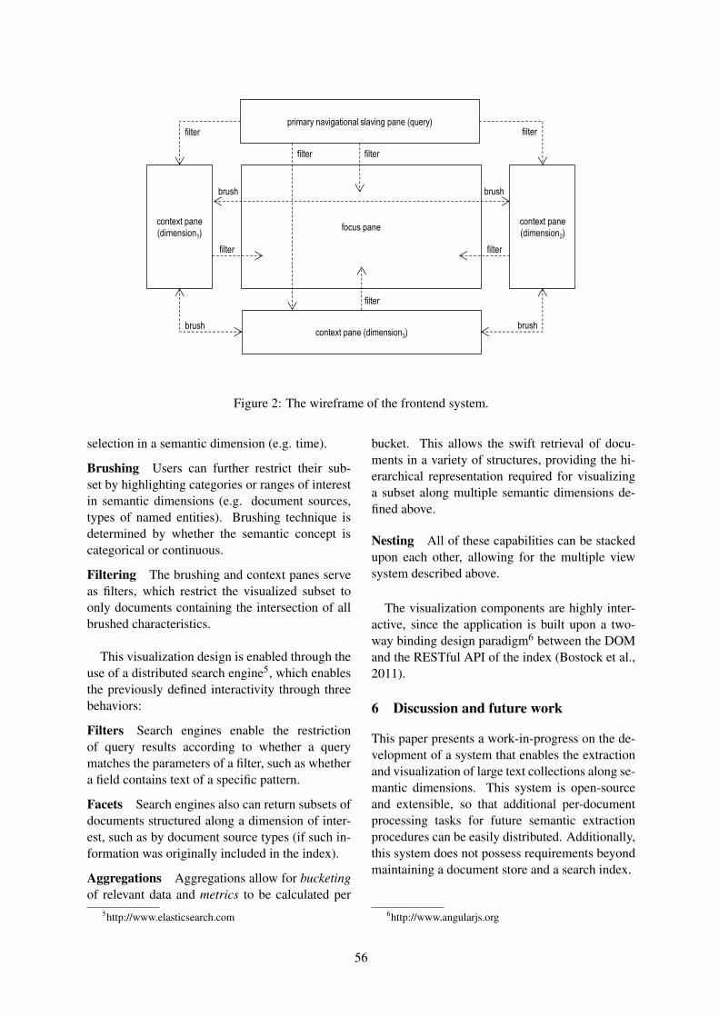
focus pane context pane
(dimension2)
context pane
(dimension1)
context pane (dimension3)
primary navigational slaving pane (query)
brush brush
filter filter
filter
filter
filter filter
brush brush
filter
Figure 2: The wireframe of the frontend system.
selection in a semantic dimension (e.g. time).
Brushing Users can further restrict their sub-set by highlighting categories or ranges of interestin semantic dimensions (e.g. document sources,types of named entities). Brushing technique isdetermined by whether the semantic concept iscategorical or continuous.
Filtering The brushing and context panes serveas filters, which restrict the visualized subset toonly documents containing the intersection of allbrushed characteristics.
This visualization design is enabled through theuse of a distributed search engine5, which enablesthe previously defined interactivity through threebehaviors:
Filters Search engines enable the restrictionof query results according to whether a querymatches the parameters of a filter, such as whethera field contains text of a specific pattern.
Facets Search engines also can return subsets ofdocuments structured along a dimension of inter-est, such as by document source types (if such in-formation was originally included in the index).
Aggregations Aggregations allow for bucketingof relevant data and metrics to be calculated per
5http://www.elasticsearch.com
bucket. This allows the swift retrieval of docu-ments in a variety of structures, providing the hi-erarchical representation required for visualizinga subset along multiple semantic dimensions de-fined above.
Nesting All of these capabilities can be stackedupon each other, allowing for the multiple viewsystem described above.
The visualization components are highly inter-active, since the application is built upon a two-way binding design paradigm6 between the DOMand the RESTful API of the index (Bostock et al.,2011).
6 Discussion and future work
This paper presents a work-in-progress on the de-velopment of a system that enables the extractionand visualization of large text collections along se-mantic dimensions. This system is open-sourceand extensible, so that additional per-documentprocessing tasks for future semantic extractionprocedures can be easily distributed. Additionally,this system does not possess requirements beyondmaintaining a document store and a search index.
6http://www.angularjs.org
56
ReferencesRie Kubota Ando, Branimir K Boguraev, Roy J Byrd,
and Mary S Neff. 2000. Multi-document summa-rization by visualizing topical content. In Proceed-ings of the 2000 NAACL-ANLP Workshop on Auto-matic Summarization, pages 79–98. Association forComputational Linguistics.
Roi Blanco, Harry Halpin, Daniel M Herzig, Pe-ter Mika, Jeffrey Pound, Henry S Thompson, andT Tran Duc. 2011. Entity search evaluation overstructured web data. In Proceedings of the 1st inter-national workshop on entity-oriented search work-shop (SIGIR 2011), ACM, New York.
Michael Bostock, Vadim Ogievetsky, and Jeffrey Heer.2011. D3 data-driven documents. Visualizationand Computer Graphics, IEEE Transactions on,17(12):2301–2309.
Penny Chase, Ray D’Amore, Nahum Gershon, RodHolland, Rob Hyland, Inderjeet Mani, Mark May-bury, Andy Merlino, and Jim Rayson. 1998. Se-mantic visualization. In ACL-COLING Workshopon Content Visualization and Intermedia Represen-tation.
Jason Chuang, Daniel Ramage, Christopher Manning,and Jeffrey Heer. 2012. Interpretation and trust:Designing model-driven visualizations for text anal-ysis. In Proceedings of the SIGCHI Conference onHuman Factors in Computing Systems, pages 443–452. ACM.
Marie-Catherine De Marneffe, Bill MacCartney,Christopher D Manning, et al. 2006. Generat-ing typed dependency parses from phrase structureparses. In Proceedings of LREC, volume 6, pages449–454.
Jenny Rose Finkel, Trond Grenager, and ChristopherManning. 2005. Incorporating non-local informa-tion into information extraction systems by gibbssampling. In Proceedings of the 43rd Annual Meet-ing on Association for Computational Linguistics,pages 363–370. Association for Computational Lin-guistics.
Danyel Fisher, Aaron Hoff, George Robertson, andMatthew Hurst. 2008. Narratives: A visualizationto track narrative events as they develop. In VisualAnalytics Science and Technology, 2008. VAST’08.IEEE Symposium on, pages 115–122. IEEE.
Ramanathan Guha, Rob McCool, and Eric Miller.2003. Semantic search. In Proceedings of the 12thinternational conference on World Wide Web, pages700–709. ACM.
Marti A Hearst and Chandu Karadi. 1997. Cat-a-cone:an interactive interface for specifying searches andviewing retrieval results using a large category hi-erarchy. In ACM SIGIR Forum, volume 31, pages246–255. ACM.
Marti A Hearst. 1995. Tilebars: visualization of termdistribution information in full text information ac-cess. In Proceedings of the SIGCHI conference onHuman factors in computing systems, pages 59–66.ACM Press/Addison-Wesley Publishing Co.
Marti A Hearst. 1999a. Untangling text data mining.In Proceedings of the 37th annual meeting of theAssociation for Computational Linguistics on Com-putational Linguistics, pages 3–10. Association forComputational Linguistics.
Marti A Hearst. 1999b. The use of categories andclusters for organizing retrieval results. In Natu-ral language information retrieval, pages 333–374.Springer.
Heeyoung Lee, Yves Peirsman, Angel Chang,Nathanael Chambers, Mihai Surdeanu, and Dan Ju-rafsky. 2011. Stanford’s multi-pass sieve coref-erence resolution system at the conll-2011 sharedtask. In Proceedings of the Fifteenth Conference onComputational Natural Language Learning: SharedTask, pages 28–34. Association for ComputationalLinguistics.
Heeyoung Lee, Angel Chang, Yves Peirsman,Nathanael Chambers, Mihai Surdeanu, and Dan Ju-rafsky. 2013. Deterministic coreference resolutionbased on entity-centric, precision-ranked rules.
Shixia Liu, Michelle X Zhou, Shimei Pan, WeihongQian, Weijia Cai, and Xiaoxiao Lian. 2009. Interac-tive, topic-based visual text summarization and anal-ysis. In Proceedings of the 18th ACM conferenceon Information and knowledge management, pages543–552. ACM.
Christopher Manning and Dan Klein. 2003. Opti-mization, maxent models, and conditional estima-tion without magic. In Proceedings of the 2003 Con-ference of the North American Chapter of the As-sociation for Computational Linguistics on HumanLanguage Technology: Tutorials-Volume 5, pages8–8. Association for Computational Linguistics.
Daan Odijk, Ork de Rooij, Maria-Hendrike Peetz,Toine Pieters, Maarten de Rijke, and StephenSnelders. 2012. Semantic document selection.In Theory and Practice of Digital Libraries, pages215–221. Springer.
Jeffrey Pound, Peter Mika, and Hugo Zaragoza. 2010.Ad-hoc object retrieval in the web of data. In Pro-ceedings of the 19th international conference onWorld wide web, pages 771–780. ACM.
Karthik Raghunathan, Heeyoung Lee, Sudarshan Ran-garajan, Nathanael Chambers, Mihai Surdeanu, DanJurafsky, and Christopher Manning. 2010. A multi-pass sieve for coreference resolution. In Proceed-ings of the 2010 Conference on Empirical Methodsin Natural Language Processing, pages 492–501.Association for Computational Linguistics.
57
Daniel Ramage, Evan Rosen, Jason Chuang, Christo-pher D Manning, and Daniel A McFarland. 2009.Topic modeling for the social sciences. In NIPS2009 Workshop on Applications for Topic Models:Text and Beyond, volume 5.
Marta Recasens, Marie-Catherine de Marneffe, andChristopher Potts. 2013. The life and death of dis-course entities: Identifying singleton mentions. InProceedings of the 2013 Conference of the NorthAmerican Chapter of the Association for Computa-tional Linguistics: Human Language Technologies,pages 627–633.
Richard Socher, Alex Perelygin, Jean Y Wu, JasonChuang, Christopher D Manning, Andrew Y Ng,and Christopher Potts. 2013. Recursive deep mod-els for semantic compositionality over a sentimenttreebank. In Proceedings of the Conference on Em-pirical Methods in Natural Language Processing(EMNLP), pages 1631–1642.
Kristina Toutanova, Dan Klein, Christopher D Man-ning, and Yoram Singer. 2003. Feature-rich part-of-speech tagging with a cyclic dependency network.In Proceedings of the 2003 Conference of the NorthAmerican Chapter of the Association for Computa-tional Linguistics on Human Language Technology-Volume 1, pages 173–180. Association for Compu-tational Linguistics.
Michelle Q Wang Baldonado, Allison Woodruff, andAllan Kuchinsky. 2000. Guidelines for using multi-ple views in information visualization. In Proceed-ings of the working conference on Advanced visualinterfaces, pages 110–119. ACM.
58
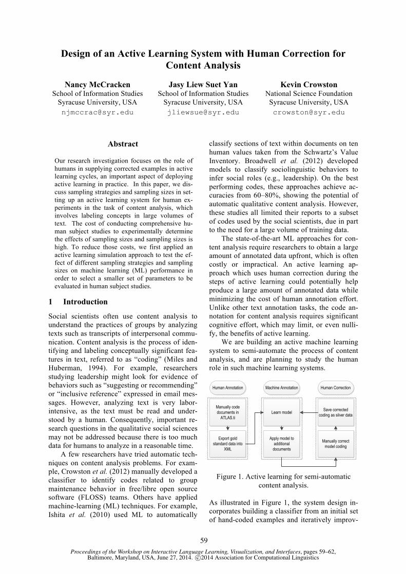
Proceedings of the Workshop on Interactive Language Learning, Visualization, and Interfaces, pages 59–62,Baltimore, Maryland, USA, June 27, 2014. c©2014 Association for Computational Linguistics
Design of an Active Learning System with Human Correction for Content Analysis
Nancy McCracken
School of Information Studies Syracuse University, USA [email protected]
Jasy Liew Suet Yan School of Information Studies
Syracuse University, USA [email protected]
Kevin Crowston National Science Foundation
Syracuse University, USA [email protected]
Abstract
Our research investigation focuses on the role of humans in supplying corrected examples in active learning cycles, an important aspect of deploying active learning in practice. In this paper, we dis-cuss sampling strategies and sampling sizes in set-ting up an active learning system for human ex-periments in the task of content analysis, which involves labeling concepts in large volumes of text. The cost of conducting comprehensive hu-man subject studies to experimentally determine the effects of sampling sizes and sampling sizes is high. To reduce those costs, we first applied an active learning simulation approach to test the ef-fect of different sampling strategies and sampling sizes on machine learning (ML) performance in order to select a smaller set of parameters to be evaluated in human subject studies.
1 Introduction
Social scientists often use content analysis to understand the practices of groups by analyzing texts such as transcripts of interpersonal commu-nication. Content analysis is the process of iden-tifying and labeling conceptually significant fea-tures in text, referred to as “coding” (Miles and Huberman, 1994). For example, researchers studying leadership might look for evidence of behaviors such as “suggesting or recommending” or “inclusive reference” expressed in email mes-sages. However, analyzing text is very labor-intensive, as the text must be read and under-stood by a human. Consequently, important re-search questions in the qualitative social sciences may not be addressed because there is too much data for humans to analyze in a reasonable time.
A few researchers have tried automatic tech-niques on content analysis problems. For exam-ple, Crowston et al. (2012) manually developed a classifier to identify codes related to group maintenance behavior in free/libre open source software (FLOSS) teams. Others have applied machine-learning (ML) techniques. For example, Ishita et al. (2010) used ML to automatically
classify sections of text within documents on ten human values taken from the Schwartz’s Value Inventory. Broadwell et al. (2012) developed models to classify sociolinguistic behaviors to infer social roles (e.g., leadership). On the best performing codes, these approaches achieve ac-curacies from 60–80%, showing the potential of automatic qualitative content analysis. However, these studies all limited their reports to a subset of codes used by the social scientists, due in part to the need for a large volume of training data.
The state-of-the-art ML approaches for con-tent analysis require researchers to obtain a large amount of annotated data upfront, which is often costly or impractical. An active learning ap-proach which uses human correction during the steps of active learning could potentially help produce a large amount of annotated data while minimizing the cost of human annotation effort. Unlike other text annotation tasks, the code an-notation for content analysis requires significant cognitive effort, which may limit, or even nulli-fy, the benefits of active learning.
We are building an active machine learning system to semi-automate the process of content analysis, and are planning to study the human role in such machine learning systems.
Manually code documents in
ATLAS.ti
Export gold standard data into
XML
Human Annotation Machine Annotation
Learn model
Apply model to additional
documents
Human Correction
Manually correct model coding
Save corrected coding as silver data
Figure 1. Active learning for semi-automatic
content analysis.
As illustrated in Figure 1, the system design in-corporates building a classifier from an initial set of hand-coded examples and iteratively improv-
59
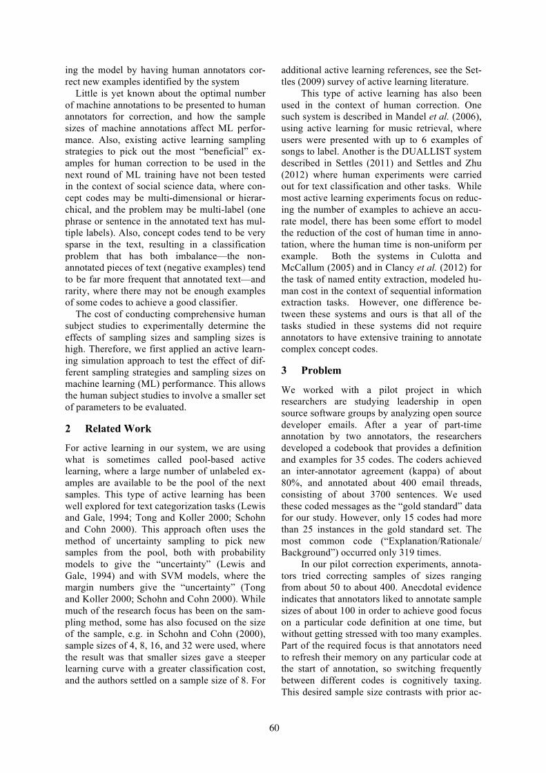
ing the model by having human annotators cor-rect new examples identified by the system
Little is yet known about the optimal number of machine annotations to be presented to human annotators for correction, and how the sample sizes of machine annotations affect ML perfor-mance. Also, existing active learning sampling strategies to pick out the most “beneficial” ex-amples for human correction to be used in the next round of ML training have not been tested in the context of social science data, where con-cept codes may be multi-dimensional or hierar-chical, and the problem may be multi-label (one phrase or sentence in the annotated text has mul-tiple labels). Also, concept codes tend to be very sparse in the text, resulting in a classification problem that has both imbalance—the non-annotated pieces of text (negative examples) tend to be far more frequent that annotated text—and rarity, where there may not be enough examples of some codes to achieve a good classifier.
The cost of conducting comprehensive human subject studies to experimentally determine the effects of sampling sizes and sampling sizes is high. Therefore, we first applied an active learn-ing simulation approach to test the effect of dif-ferent sampling strategies and sampling sizes on machine learning (ML) performance. This allows the human subject studies to involve a smaller set of parameters to be evaluated.
2 Related Work
For active learning in our system, we are using what is sometimes called pool-based active learning, where a large number of unlabeled ex-amples are available to be the pool of the next samples. This type of active learning has been well explored for text categorization tasks (Lewis and Gale, 1994; Tong and Koller 2000; Schohn and Cohn 2000). This approach often uses the method of uncertainty sampling to pick new samples from the pool, both with probability models to give the “uncertainty” (Lewis and Gale, 1994) and with SVM models, where the margin numbers give the “uncertainty” (Tong and Koller 2000; Schohn and Cohn 2000). While much of the research focus has been on the sam-pling method, some has also focused on the size of the sample, e.g. in Schohn and Cohn (2000), sample sizes of 4, 8, 16, and 32 were used, where the result was that smaller sizes gave a steeper learning curve with a greater classification cost, and the authors settled on a sample size of 8. For
additional active learning references, see the Set-tles (2009) survey of active learning literature.
This type of active learning has also been used in the context of human correction. One such system is described in Mandel et al. (2006), using active learning for music retrieval, where users were presented with up to 6 examples of songs to label. Another is the DUALLIST system described in Settles (2011) and Settles and Zhu (2012) where human experiments were carried out for text classification and other tasks. While most active learning experiments focus on reduc-ing the number of examples to achieve an accu-rate model, there has been some effort to model the reduction of the cost of human time in anno-tation, where the human time is non-uniform per example. Both the systems in Culotta and McCallum (2005) and in Clancy et al. (2012) for the task of named entity extraction, modeled hu-man cost in the context of sequential information extraction tasks. However, one difference be-tween these systems and ours is that all of the tasks studied in these systems did not require annotators to have extensive training to annotate complex concept codes.
3 Problem
We worked with a pilot project in which researchers are studying leadership in open source software groups by analyzing open source developer emails. After a year of part-time annotation by two annotators, the researchers developed a codebook that provides a definition and examples for 35 codes. The coders achieved an inter-annotator agreement (kappa) of about 80%, and annotated about 400 email threads, consisting of about 3700 sentences. We used these coded messages as the “gold standard” data for our study. However, only 15 codes had more than 25 instances in the gold standard set. The most common code (“Explanation/Rationale/ Background”) occurred only 319 times.
In our pilot correction experiments, annota-tors tried correcting samples of sizes ranging from about 50 to about 400. Anecdotal evidence indicates that annotators liked to annotate sample sizes of about 100 in order to achieve good focus on a particular code definition at one time, but without getting stressed with too many examples. Part of the required focus is that annotators need to refresh their memory on any particular code at the start of annotation, so switching frequently between different codes is cognitively taxing. This desired sample size contrasts with prior ac-
60
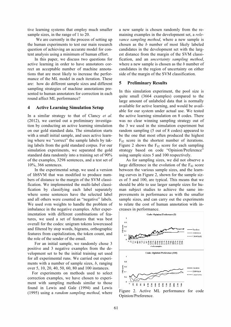
tive learning systems that employ much smaller sample sizes, in the range of 1 to 20.
We are currently in the process of setting up the human experiments to test our main research question of achieving an accurate model for con-tent analysis using a minimum of human effort.
In this paper, we discuss two questions for active learning in order to have annotators cor-rect an acceptable number of machine annota-tions that are most likely to increase the perfor-mance of the ML model in each iteration. These are: how do different sample sizes and different sampling strategies of machine annotations pre-sented to human annotators for correction in each round affect ML performance?
4 Active Learning Simulation Setup
In a similar strategy to that of Clancy et al. (2012), we carried out a preliminary investiga-tion by conducting an active learning simulation on our gold standard data. The simulation starts with a small initial sample, and uses active learn-ing where we “correct” the sample labels by tak-ing labels from the gold standard corpus. For our simulation experiments, we separated the gold standard data randomly into a training set of 90% of the examples, 3298 sentences, and a test set of 10%, 366 sentences.
In the experimental setup, we used a version of libSVM that was modified to produce num-bers of distance to the margin of the SVM classi-fication. We implemented the multi-label classi-fication by classifying each label separately where some sentences have the selected label and all others were counted as “negative” labels. We used svm weights to handle the problem of imbalance in the negative examples. After exper-imentation with different combinations of fea-tures, we used a set of features that was best overall for the codes: unigram tokens lowercased and filtered by stop words, bigrams, orthographic features from capitalization, the token count, and the role of the sender of the email.
For an initial sample, we randomly chose 3 positive and 3 negative examples from the de-velopment set to be the initial training set used for all experimental runs. We carried out experi-ments with a number of sample sizes, b, ranging over 5, 10, 20, 40, 50, 60, 80 and 100 instances.
For experiments on methods used to select correction examples, we have chosen to experi-ment with sampling methods similar to those found in Lewis and Gale (1994) and Lewis (1995) using a random sampling method, where
a new sample is chosen randomly from the re-maining examples in the development set, a rele-vance sampling method, where a new sample is chosen as the b number of most likely labeled candidates in the development set with the larg-est distance from the margin of the SVM classi-fication, and an uncertainty sampling method, where a new sample is chosen as the b number of candidates in the region of uncertainty on either side of the margin of the SVM classification.
5 Preliminary Results
In this simulation experiment, the pool size is quite small (3664 examples) compared to the large amount of unlabeled data that is normally available for active learning, and would be avail-able for our system under actual use. We tested the active learning simulation on 8 codes. There was no clear winning sampling strategy out of the 3 we used in the simulation experiment but random sampling (5 out of 8 codes) appeared to be the one that most often produced the highest Fß2 score in the shortest number of iterations. Figure 2 shows the Fß2 score for each sampling strategy based on code “Opinion/Preference” using sample sizes 5 and 100 respectively.
As for sampling sizes, we did not observe a large difference in the evolution of the Fß2 score between the various sample sizes, and the learn-ing curves in Figure 2, shown for the sample siz-es of 5 and 100, are typical. This means that we should be able to use larger sample sizes for hu-man subject studies to achieve the same im-provements in performance as with the smaller sample sizes, and can carry out the experiments to relate the cost of human annotation with in-creases in performance.
Figure 2. Active ML performance for code Opinion/Preference.
61
6 Conclusion and Future Work
Our findings are inconclusive as we have yet to run the active learning simulations on all the codes. However, preliminary results are directing us towards using larger sample sizes and then experimenting with random and uncertainty sampling in the human subject studies.
From our experiments with the different codes, we found the performance on less fre-quent codes to be problematic as it is difficult for the active learning system to identify potential positive examples to improve the models. While the system performance may improve to handle such sparse cases, it may be better to modify the codebook instead. We plan to give the user feed-back on the performance of the codes at each iteration of the active learning and support modi-fications to the codebook, for example, the user may wish to drop some codes or collapse them according to some hierarchy. After all, if a code is not found in the text, it is hard to argue for its theoretical importance.
We are currently completing the design of the parameters of the active learning process for the human correction experiments on our pilot project with the codes about leadership in open source software groups. We will also be testing and undergoing further development of the user interface for the annotators.
Our next step will be to test the system on other projects with other researchers. We hope to gain more insight into what types of coding schemes and codes are easier to learn than oth-ers, and to be able to guide social scientists into developing coding schemes that are not only based on the social science theory but also useful in practice to develop an accurate classifier for very large amounts of digital text. Acknowledgements:
This material is based upon work supported by the National Science Foundation under Grant No. IIS-1111107. Kevin Crowston is supported by the National Science Foundation. Any opin-ions, findings, and conclusions or recommenda-tions expressed in this material are those of the author(s) and do not necessarily reflect the views of the National Science Foundation. The authors gratefully acknowledge helpful suggestions by the reviewers.
Reference Broadwell, G. A., Stromer-Galley, J., Strzalkowski,
T., Shaikh, S., Taylor, S., Liu, T., Boz, U., Elia, A., Jiao, L., & Webb, N. (2013). Modeling sociocul-tural phenomena in discourse. Natural Language Engineering, 19(02), 213–257.
Clancy, S., Bayer, S. and Kozierok, R. (2012) “Ac-tive Learning with a Human In The Loop,” Mitre Corporation.
Crowston, K., Allen, E. E., & Heckman, R. (2012). Using natural language processing technology for qualitative data analysis. International Journal of Social Research Methodology, 15(6), 523–543.
Culotta, A. and McCallum, A. (2005) “Reducing La-beling Effort for Structured Prediction Tasks.”
Ishita, E., Oard, D. W., Fleischmann, K. R., Cheng, A.-S., & Templeton, T. C. (2010). Investigating multi-label classification for human values. Pro-ceedings of the American Society for Information Science and Technology, 47(1), 1–4.
Miles, M. B., & Huberman, A. M. (1994). Qualitative data analysis: An expanded sourcebook. Sage Pub-lications.
Lewis, D. D., & Gale, W. A. (1994). A sequential algorithm for training text classifiers. In Proceed-ings of the 17th annual international ACM SIGIR conference on Research and development in infor-mation retrieval (pp. 3-12).
Lewis, D. D. (1995). A sequential algorithm for train-ing text classifiers: Corrigendum and additional da-ta. In ACM SIGIR Forum (Vol. 29, No. 2, pp. 13-19).
Mandel, M. I., Poliner, G. E., & Ellis, D. P. (2006). Support vector machine active learning for music retrieval. Multimedia systems, 12(1), 3-13.
Schohn, G., & Cohn, D. (2000). Less is more: Active learning with support vector machines. In Interna-tional Conference on Machine Learning (pp. 839-846).
Settles, B. (2010). Active learning literature survey. University of Wisconsin, Madison, 52, 55-66.
Settles, B. (2011). Closing the loop: Fast, interactive semi-supervised annotation with queries on fea-tures and instances. In Proceedings of the Confer-ence on Empirical Methods in Natural Language Processing (pp. 1467-1478).
Settles, B., & Zhu, X. (2012). Behavioral factors in interactive training of text classifiers. In Proceed-ings of the 2012 Conference of the North American Chapter of the Association for Computational Lin-guistics: Human Language Technologies (pp. 563-567).
Tong, S., & Koller, D. (2002). Support vector ma-chine active learning with applications to text clas-sification. The Journal of Machine Learning Re-search, 2, 45-66.
62
Proceedings of the Workshop on Interactive Language Learning, Visualization, and Interfaces, pages 63–70,Baltimore, Maryland, USA, June 27, 2014. c©2014 Association for Computational Linguistics
LDAvis: A method for visualizing and interpreting topics
Carson SievertIowa State University3414 Snedecor Hall
Ames, IA 50014, [email protected]
Kenneth E. ShirleyAT&T Labs Research
33 Thomas Street, 26th FloorNew York, NY 10007, USA
Abstract
We present LDAvis, a web-based interac-tive visualization of topics estimated usingLatent Dirichlet Allocation that is built us-ing a combination of R and D3. Our visu-alization provides a global view of the top-ics (and how they differ from each other),while at the same time allowing for a deepinspection of the terms most highly asso-ciated with each individual topic. First,we propose a novel method for choosingwhich terms to present to a user to aid inthe task of topic interpretation, in whichwe define the relevance of a term to atopic. Second, we present results from auser study that suggest that ranking termspurely by their probability under a topic issuboptimal for topic interpretation. Last,we describe LDAvis, our visualizationsystem that allows users to flexibly exploretopic-term relationships using relevance tobetter understand a fitted LDA model.
1 Introduction
Recently much attention has been paid to visual-izing the output of topic models fit using LatentDirichlet Allocation (LDA) (Gardner et al., 2010;Chaney and Blei, 2012; Chuang et al., 2012b; Gre-tarsson et al., 2011). Such visualizations are chal-lenging to create because of the high dimensional-ity of the fitted model – LDA is typically appliedto many thousands of documents, which are mod-eled as mixtures of dozens (or hundreds) of top-ics, which themselves are modeled as distributionsover thousands of terms (Blei et al., 2003; Griffithsand Steyvers, 2004). The most promising basictechnique for creating LDA visualizations that areboth compact and thorough is interactivity.
We introduce an interactive visualization sys-tem that we call LDAvis that attempts to answer
a few basic questions about a fitted topic model:(1) What is the meaning of each topic?, (2) Howprevalent is each topic?, and (3) How do the topicsrelate to each other? Different visual componentsanswer each of these questions, some of which areoriginal, and some of which are borrowed from ex-isting tools.
Our visualization (illustrated in Figure 1) hastwo basic pieces. First, the left panel of our visual-ization presents a global view of the topic model,and answers questions 2 and 3. In this view, weplot the topics as circles in the two-dimensionalplane whose centers are determined by comput-ing the distance between topics, and then by us-ing multidimensional scaling to project the inter-topic distances onto two dimensions, as is donein (Chuang et al., 2012a). We encode each topic’soverall prevalence using the areas of the circles,where we sort the topics in decreasing order ofprevalence.
Second, the right panel of our visualization de-picts a horizontal barchart whose bars representthe individual terms that are the most useful for in-terpreting the currently selected topic on the left,and allows users to answer question 1, “What isthe meaning of each topic?”. A pair of overlaidbars represent both the corpus-wide frequency ofa given term as well as the topic-specific frequencyof the term, as in (Chuang et al., 2012b).
The left and right panels of our visualization arelinked such that selecting a topic (on the left) re-veals the most useful terms (on the right) for inter-preting the selected topic. In addition, selecting aterm (on the right) reveals the conditional distribu-tion over topics (on the left) for the selected term.This kind of linked selection allows users to exam-ine a large number of topic-term relationships in acompact manner.
A key innovation of our system is how we deter-mine the most useful terms for interpreting a giventopic, and how we allow users to interactively ad-
63
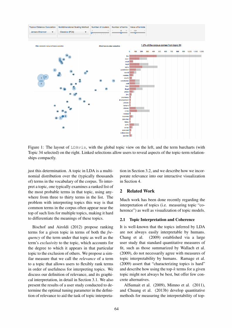
Figure 1: The layout of LDAvis, with the global topic view on the left, and the term barcharts (withTopic 34 selected) on the right. Linked selections allow users to reveal aspects of the topic-term relation-ships compactly.
just this determination. A topic in LDA is a multi-nomial distribution over the (typically thousandsof) terms in the vocabulary of the corpus. To inter-pret a topic, one typically examines a ranked list ofthe most probable terms in that topic, using any-where from three to thirty terms in the list. Theproblem with interpreting topics this way is thatcommon terms in the corpus often appear near thetop of such lists for multiple topics, making it hardto differentiate the meanings of these topics.
Bischof and Airoldi (2012) propose rankingterms for a given topic in terms of both the fre-quency of the term under that topic as well as theterm’s exclusivity to the topic, which accounts forthe degree to which it appears in that particulartopic to the exclusion of others. We propose a sim-ilar measure that we call the relevance of a termto a topic that allows users to flexibly rank termsin order of usefulness for interpreting topics. Wediscuss our definition of relevance, and its graphi-cal interpretation, in detail in Section 3.1. We alsopresent the results of a user study conducted to de-termine the optimal tuning parameter in the defini-tion of relevance to aid the task of topic interpreta-
tion in Section 3.2, and we describe how we incor-porate relevance into our interactive visualizationin Section 4.
2 Related Work
Much work has been done recently regarding theinterpretation of topics (i.e. measuring topic “co-herence”) as well as visualization of topic models.
2.1 Topic Interpretation and Coherence
It is well-known that the topics inferred by LDAare not always easily interpretable by humans.Chang et al. (2009) established via a largeuser study that standard quantitative measures offit, such as those summarized by Wallach et al.(2009), do not necessarily agree with measures oftopic interpretability by humans. Ramage et al.(2009) assert that “characterizing topics is hard”and describe how using the top-k terms for a giventopic might not always be best, but offer few con-crete alternatives.
AlSumait et al. (2009), Mimno et al. (2011),and Chuang et al. (2013b) develop quantitativemethods for measuring the interpretability of top-
64
ics based on experiments with data sets that comewith some notion of topical ground truth, such asdocument metadata or expert-created topic labels.These methods are useful for understanding, in aglobal sense, which topics are interpretable (andwhy), but they don’t specifically attempt to aid theuser in interpreting individual topics.
Blei and Lafferty (2009) developed “Turbo Top-ics”, a method of identifying n-grams within LDA-inferred topics that, when listed in decreasing or-der of probability, provide users with extra in-formation about the usage of terms within top-ics. This two-stage process yields good results onexperimental data, although the resulting outputis still simply a ranked list containing a mixtureof terms and n-grams, and the usefulness of themethod for topic interpretation was not tested in auser study.
Newman et al. (2010) describe a method forranking terms within topics to aid interpretabilitycalled Pointwise Mutual Information (PMI) rank-ing. Under PMI ranking of terms, each of the tenmost probable terms within a topic are ranked indecreasing order of approximately how often theyoccur in close proximity to the nine other mostprobable terms from that topic in some large, ex-ternal “reference” corpus, such as Wikipedia orGoogle n-grams. Although this method correlatedhighly with human judgments of term importancewithin topics, it does not easily generalize to topicmodels fit to corpora that don’t have a readilyavailable external source of word co-occurrences.
In contrast, Taddy (2011) uses an intrinsic mea-sure to rank terms within topics: a quantity calledlift, defined as the ratio of a term’s probabilitywithin a topic to its marginal probability acrossthe corpus. This generally decreases the rankingsof globally frequent terms, which can be helpful.We find that it can be noisy, however, by givinghigh rankings to very rare terms that occur in onlya single topic, for instance. While such terms maycontain useful topical content, if they are very rarethe topic may remain difficult to interpret.
Finally, Bischof and Airoldi (2012) develop andimplement a new statistical topic model that infersboth a term’s frequency as well as its exclusivity– the degree to which its occurrences are limitedto only a few topics. They introduce a univari-ate measure called a FREX score (“FRequencyand EXclusivity”) which is a weighted harmonicmean of a term’s rank within a given topic with
respect to frequency and exclusivity, and they rec-ommend it as a way to rank terms to aid topic in-terpretation. We propose a similar method that isa weighted average of the logarithms of a term’sprobability and its lift, and we justify it with a userstudy and incorporate it into our interactive visu-alization.
2.2 Topic Model Visualization Systems
A number of visualization systems for topic mod-els have been developed in recent years. Sev-eral of them focus on allowing users to browsedocuments, topics, and terms to learn about therelationships between these three canonical topicmodel units (Gardner et al., 2010; Chaney andBlei, 2012; Snyder et al., 2013). These browserstypically use lists of the most probable termswithin topics to summarize the topics, and the vi-sualization elements are limited to barcharts orword clouds of term probabilities for each topic,pie charts of topic probabilities for each document,and/or various barcharts or scatterplots related todocument metadata. Although these tools can beuseful for browsing a corpus, we seek a more com-pact visualization, with the more narrow focus ofquickly and easily understanding the individualtopics themselves (without necessarily visualizingdocuments).
Chuang et al. (2012b) develop such a tool,called “Termite”, which visualizes the set of topic-term distributions estimated in LDA using a ma-trix layout. The authors introduce two measuresof the usefulness of terms for understanding atopic model: distinctiveness and saliency. Thesequantities measure how much information a termconveys about topics by computing the Kullback-Liebler divergence between the distribution of top-ics given the term and the marginal distributionof topics (distinctiveness), optionally weightedby the term’s overall frequency (saliency). Theauthors recommend saliency as a thresholdingmethod for selecting which terms are included inthe visualization, and they further use a seriationmethod for ordering the most salient terms to high-light differences between topics.
Termite is a compact, intuitive interactive visu-alization of the topics in a topic model, but by onlyincluding terms that rank high in saliency or dis-tinctiveness, which are global properties of terms,it is restricted to providing a global view of themodel, rather than allowing a user to deeply in-
65
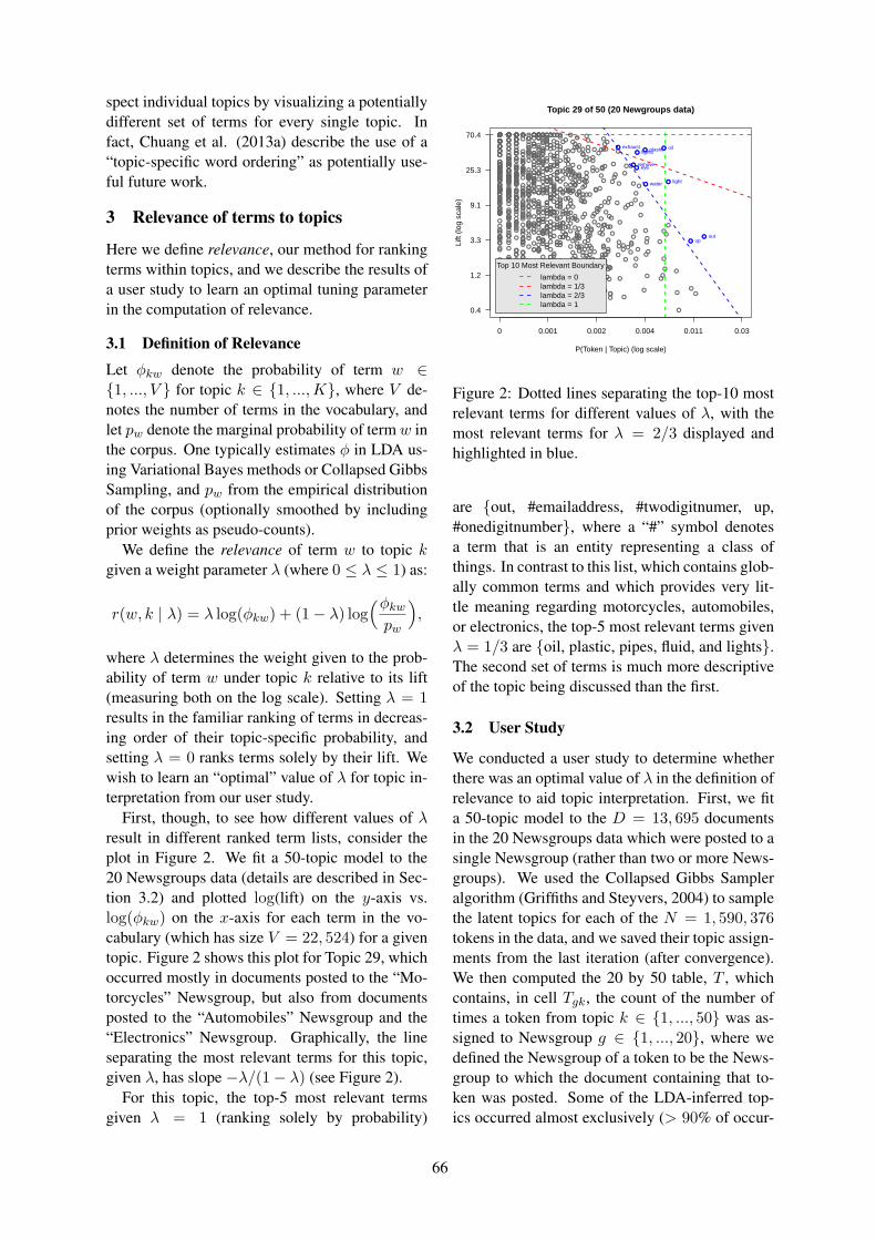
spect individual topics by visualizing a potentiallydifferent set of terms for every single topic. Infact, Chuang et al. (2013a) describe the use of a“topic-specific word ordering” as potentially use-ful future work.
3 Relevance of terms to topics
Here we define relevance, our method for rankingterms within topics, and we describe the results ofa user study to learn an optimal tuning parameterin the computation of relevance.
3.1 Definition of Relevance
Let φkw denote the probability of term w ∈{1, ..., V } for topic k ∈ {1, ...,K}, where V de-notes the number of terms in the vocabulary, andlet pw denote the marginal probability of termw inthe corpus. One typically estimates φ in LDA us-ing Variational Bayes methods or Collapsed GibbsSampling, and pw from the empirical distributionof the corpus (optionally smoothed by includingprior weights as pseudo-counts).
We define the relevance of term w to topic kgiven a weight parameter λ (where 0 ≤ λ ≤ 1) as:
r(w, k | λ) = λ log(φkw) + (1− λ) log(φkw
pw
),
where λ determines the weight given to the prob-ability of term w under topic k relative to its lift(measuring both on the log scale). Setting λ = 1results in the familiar ranking of terms in decreas-ing order of their topic-specific probability, andsetting λ = 0 ranks terms solely by their lift. Wewish to learn an “optimal” value of λ for topic in-terpretation from our user study.
First, though, to see how different values of λresult in different ranked term lists, consider theplot in Figure 2. We fit a 50-topic model to the20 Newsgroups data (details are described in Sec-tion 3.2) and plotted log(lift) on the y-axis vs.log(φkw) on the x-axis for each term in the vo-cabulary (which has size V = 22, 524) for a giventopic. Figure 2 shows this plot for Topic 29, whichoccurred mostly in documents posted to the “Mo-torcycles” Newsgroup, but also from documentsposted to the “Automobiles” Newsgroup and the“Electronics” Newsgroup. Graphically, the lineseparating the most relevant terms for this topic,given λ, has slope −λ/(1− λ) (see Figure 2).
For this topic, the top-5 most relevant termsgiven λ = 1 (ranking solely by probability)
●
●●
●
●
●
●
●
●
●
●
●
●
●
●
●●●
●
●
●●
●
●
●
●
●
●
●
●●
●
●
●
●
●
●
●●
●
●
●
●
●
●
●
●
●
●
●
●●
●
●
●●
●
●●
●
●
●
●
●
●
●
●
●
●●
●●
●
●
●
●
●
●●
●
●
●●
●●
●
●
●
●
●
●
●●
●
●
●
●●
●
●
●
●
●
●
●
●
●
●
●
●●
●
●
●
●
●
●
●
●
●
●
●
●
●
●
●
●
●
●
●
●
●
●
●
●●
●
●
●
●●
●
●
●
●
●
●●
●
●●
●
●
●
●
●
●
●
●●
●
●●
●●
●
●
●
●
●●●
●
●
●
●
●
●●●
●
●
●●
●
●
●
●
●
●
●
●
●
●
●
●
●●
●
●
●●
●
●
●
●
●
●●
●
●
●
●
●●●
●
●
●
●
●
●
●
●
●
●
●
●
●
●
●
●
●
●
●
●
●
●
●●
●
●
●
●
●
●
●●
●
●
●
●
●
●
●
●
●
●
●
●
●●
●●
●
●
●
●
●●
●
●
●
●
●
●
●
●
●●
●
●●
●
●
●
●
●
●
●
●
●
●
●●
●
●
●
●
●
●
●
●
●
●
●
●●
●
●
●
●
●●
●
●
●
●
●
●
●
●●
●●
●
●
●
●
●
●
●
●
●
●
●
●
●
●
●
●●
●
●●
●
●
●
●
●
●
●
●
●
●
●
●
●
●
●●
●
●
●
●
●
●
●
●
●
●●●
●
●
●●
●●
●
●
●
●
●
●
●
●
●
●●
●
●
●
●
●●
●
●
●
●
●●
●
●
●●
●
●
●
●●
●
●
●●●
●
●
●
●
●
●●●
●
●
●●
●
●
●
●
●
●
●
●
●
●
●
●
●
●
●
●
●
●
●
●
●
●
●
●
●●
●●
●
●●
●●
●
●
●
●
●●
●
●
●●
●
●●
●
●
●●
●
●
●
●
●
●
●
●
●
●
●
●●
●●●
●
●
●
●
●●
●
●●
●
●
●
●
●
●
●
●
●
●
●
●
●
●
●
●
●●●
●
●
●
●
●
●
●●
●
●
●
●
●
●
●
●
●●
●
●
●
●●
●
●
●
●
●
●
●
●
●
●
●
●
●●
●
●
●
●
●
●
●
●
●
●
●
●
●
●
●
●
●
●
●
●
●
●
●
●
●
●
●
●
●
●
●
●
●
●
●
●
●
●
●
●
●
●
●
●
●
●●
●●
●
●
●●
●
●
●
●
●
●
●●
●
●
●
●
●
●
●
●
●
●
●●
●
●
●
●●
●
●
●
●
●
●
●
●●
●●
●
●●
●●
●
●
●
●
●
●
●
●
●
●
●
●
●
●
●●
●
●
●
●
●
●●
●
●
●
●
●
●●●
●
●
●
●
●
●●
●
●
●
●
●
●●
●
●
●
●
●
●
●
●
●
●
●●
●
●
●
●
●●
●
●
●
●
●
●
●
●
●
●
●
●
●
●●
●●●
●
●●●
●
●●
●●
●●
●
●
●
●
●
●
●
●
●
●
●
●●
●
●●
●
●
●
●
●
●
●●
●
●
●
●
●●
●
●
●
●
●
●
●
●
●●
●●●
●
●●
●●
●●
●
●
●
●
●
●
●●
●
●
●
●
●
●
●
●●●
●
●
●●●
●
●
●●●
●
●●
●
●
●●
●
●
●
●
●
●
●●●
●
●●●
●
●
●
●
●
●
●
●●
●●
●
●
●
●
●
●
●●
●
●
●
●
●
●●
●
●
●●
●●
●●
●
●●
●
●●
●
●●
●
●
●
●
●
●
●
●
●
●
●
●
●
●
●
●
●
●●
●
●
●
●
●
●
●
●
●
●●
●●
●
●
●●
●●
●
●
●
●
●
●●
●
●
●
●●
●●●
●●
●
●
●
●
●
●
●●
●
●
●●
●●
●
●
●●
●
●
●●●●
●
●
●
●
●
●
●
●
●●
●●
●
●
●●
●●
●●
●
●●
●●
●
●●
●●●
●
●●
●
●
●
●
●●●
●●
●
●●●●
●
●●
●●
●
●●●●
●●
●
●
●
●
●
●
●
●●●●
●
●●●
●●●●
●●●●
●
●●
●
●
●
●
●●
●
●
●●●●●●●●●●●●●●●●●●●●●●●●●●●●●
P(Token | Topic) (log scale)
Lift
(log
scal
e)
0 0.001 0.002 0.004 0.011 0.03
0.4
1.2
3.3
9.1
25.3
70.4
oil
light
plastic
out
lights
up
eyeremove
water
exhaust ●
●
●
●
●
●
●●
●
●
Top 10 Most Relevant Boundary
lambda = 0lambda = 1/3lambda = 2/3lambda = 1
Topic 29 of 50 (20 Newgroups data)
Figure 2: Dotted lines separating the top-10 mostrelevant terms for different values of λ, with themost relevant terms for λ = 2/3 displayed andhighlighted in blue.
are {out, #emailaddress, #twodigitnumer, up,#onedigitnumber}, where a “#” symbol denotesa term that is an entity representing a class ofthings. In contrast to this list, which contains glob-ally common terms and which provides very lit-tle meaning regarding motorcycles, automobiles,or electronics, the top-5 most relevant terms givenλ = 1/3 are {oil, plastic, pipes, fluid, and lights}.The second set of terms is much more descriptiveof the topic being discussed than the first.
3.2 User Study
We conducted a user study to determine whetherthere was an optimal value of λ in the definition ofrelevance to aid topic interpretation. First, we fita 50-topic model to the D = 13, 695 documentsin the 20 Newsgroups data which were posted to asingle Newsgroup (rather than two or more News-groups). We used the Collapsed Gibbs Sampleralgorithm (Griffiths and Steyvers, 2004) to samplethe latent topics for each of the N = 1, 590, 376tokens in the data, and we saved their topic assign-ments from the last iteration (after convergence).We then computed the 20 by 50 table, T , whichcontains, in cell Tgk, the count of the number oftimes a token from topic k ∈ {1, ..., 50} was as-signed to Newsgroup g ∈ {1, ..., 20}, where wedefined the Newsgroup of a token to be the News-group to which the document containing that to-ken was posted. Some of the LDA-inferred top-ics occurred almost exclusively (> 90% of occur-
66
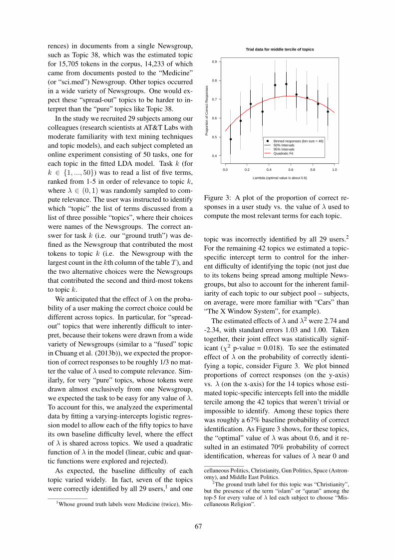
rences) in documents from a single Newsgroup,such as Topic 38, which was the estimated topicfor 15,705 tokens in the corpus, 14,233 of whichcame from documents posted to the “Medicine”(or “sci.med”) Newsgroup. Other topics occurredin a wide variety of Newsgroups. One would ex-pect these “spread-out” topics to be harder to in-terpret than the “pure” topics like Topic 38.
In the study we recruited 29 subjects among ourcolleagues (research scientists at AT&T Labs withmoderate familiarity with text mining techniquesand topic models), and each subject completed anonline experiment consisting of 50 tasks, one foreach topic in the fitted LDA model. Task k (fork ∈ {1, ..., 50}) was to read a list of five terms,ranked from 1-5 in order of relevance to topic k,where λ ∈ (0, 1) was randomly sampled to com-pute relevance. The user was instructed to identifywhich “topic” the list of terms discussed from alist of three possible “topics”, where their choiceswere names of the Newsgroups. The correct an-swer for task k (i.e. our “ground truth”) was de-fined as the Newsgroup that contributed the mosttokens to topic k (i.e. the Newsgroup with thelargest count in the kth column of the table T ), andthe two alternative choices were the Newsgroupsthat contributed the second and third-most tokensto topic k.
We anticipated that the effect of λ on the proba-bility of a user making the correct choice could bedifferent across topics. In particular, for “spread-out” topics that were inherently difficult to inter-pret, because their tokens were drawn from a widevariety of Newsgroups (similar to a “fused” topicin Chuang et al. (2013b)), we expected the propor-tion of correct responses to be roughly 1/3 no mat-ter the value of λ used to compute relevance. Sim-ilarly, for very “pure” topics, whose tokens weredrawn almost exclusively from one Newsgroup,we expected the task to be easy for any value of λ.To account for this, we analyzed the experimentaldata by fitting a varying-intercepts logistic regres-sion model to allow each of the fifty topics to haveits own baseline difficulty level, where the effectof λ is shared across topics. We used a quadraticfunction of λ in the model (linear, cubic and quar-tic functions were explored and rejected).
As expected, the baseline difficulty of eachtopic varied widely. In fact, seven of the topicswere correctly identified by all 29 users,1 and one
1Whose ground truth labels were Medicine (twice), Mis-
●
●
●
●
●●
●
●
●
●
0.0 0.2 0.4 0.6 0.8 1.0
0.4
0.5
0.6
0.7
0.8
0.9
Lambda (optimal value is about 0.6)
Pro
port
ion
of C
orre
ct R
espo
nses
Trial data for middle tercile of topics
● Binned responses (bin size = 40)50% Intervals95% IntervalsQuadratic Fit
Figure 3: A plot of the proportion of correct re-sponses in a user study vs. the value of λ used tocompute the most relevant terms for each topic.
topic was incorrectly identified by all 29 users.2
For the remaining 42 topics we estimated a topic-specific intercept term to control for the inher-ent difficulty of identifying the topic (not just dueto its tokens being spread among multiple News-groups, but also to account for the inherent famil-iarity of each topic to our subject pool – subjects,on average, were more familiar with “Cars” than“The X Window System”, for example).
The estimated effects of λ and λ2 were 2.74 and-2.34, with standard errors 1.03 and 1.00. Takentogether, their joint effect was statistically signif-icant (χ2 p-value = 0.018). To see the estimatedeffect of λ on the probability of correctly identi-fying a topic, consider Figure 3. We plot binnedproportions of correct responses (on the y-axis)vs. λ (on the x-axis) for the 14 topics whose esti-mated topic-specific intercepts fell into the middletercile among the 42 topics that weren’t trivial orimpossible to identify. Among these topics therewas roughly a 67% baseline probability of correctidentification. As Figure 3 shows, for these topics,the “optimal” value of λ was about 0.6, and it re-sulted in an estimated 70% probability of correctidentification, whereas for values of λ near 0 and
cellaneous Politics, Christianity, Gun Politics, Space (Astron-omy), and Middle East Politics.
2The ground truth label for this topic was “Christianity”,but the presence of the term “islam” or “quran” among thetop-5 for every value of λ led each subject to choose “Mis-cellaneous Religion”.
67
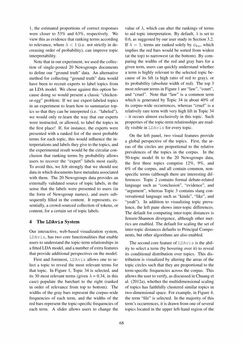
1, the estimated proportions of correct responseswere closer to 53% and 63%, respectively. Weview this as evidence that ranking terms accordingto relevance, where λ < 1 (i.e. not strictly in de-creasing order of probability), can improve topicinterpretability.
Note that in our experiment, we used the collec-tion of single-posted 20 Newsgroups documentsto define our “ground truth” data. An alternativemethod for collecting “ground truth” data wouldhave been to recruit experts to label topics froman LDA model. We chose against this option be-cause doing so would present a classic “chicken-or-egg” problem: If we use expert-labeled topicsin an experiment to learn how to summarize top-ics so that they can be interpreted (i.e. “labeled”),we would only re-learn the way that our expertswere instructed, or allowed, to label the topics inthe first place! If, for instance, the experts werepresented with a ranked list of the most probableterms for each topic, this would influence the in-terpretations and labels they give to the topics, andthe experimental result would be the circular con-clusion that ranking terms by probability allowsusers to recover the “expert” labels most easily.To avoid this, we felt strongly that we should usedata in which documents have metadata associatedwith them. The 20 Newsgroups data provides anexternally validated source of topic labels, in thesense that the labels were presented to users (inthe form of Newsgroup names), and users sub-sequently filled in the content. It represents, es-sentially, a crowd-sourced collection of tokens, orcontent, for a certain set of topic labels.
4 The LDAvis System
Our interactive, web-based visualization system,LDAvis, has two core functionalities that enableusers to understand the topic-term relationships ina fitted LDA model, and a number of extra featuresthat provide additional perspectives on the model.
First and foremost, LDAvis allows one to se-lect a topic to reveal the most relevant terms forthat topic. In Figure 1, Topic 34 is selected, andits 30 most relevant terms (given λ = 0.34, in thiscase) populate the barchart to the right (rankedin order of relevance from top to bottom). Thewidths of the gray bars represent the corpus-widefrequencies of each term, and the widths of thered bars represent the topic-specific frequencies ofeach term. A slider allows users to change the
value of λ, which can alter the rankings of termsto aid topic interpretation. By default, λ is set to0.6, as suggested by our user study in Section 3.2.If λ = 1, terms are ranked solely by φkw, whichimplies the red bars would be sorted from widest(at the top) to narrowest (at the bottom). By com-paring the widths of the red and gray bars for agiven term, users can quickly understand whethera term is highly relevant to the selected topic be-cause of its lift (a high ratio of red to gray), orits probability (absolute width of red). The top 3most relevant terms in Figure 1 are “law”, “court”,and “cruel”. Note that “law” is a common termwhich is generated by Topic 34 in about 40% ofits corpus-wide occurrences, whereas “cruel” is arelatively rare term with very high lift in Topic 34– it occurs almost exclusively in this topic. Suchproperties of the topic-term relationships are read-ily visible in LDAvis for every topic.
On the left panel, two visual features providea global perspective of the topics. First, the ar-eas of the circles are proportional to the relativeprevalences of the topics in the corpus. In the50-topic model fit to the 20 Newsgroups data,the first three topics comprise 12%, 9%, and6% of the corpus, and all contain common, non-specific terms (although there are interesting dif-ferences: Topic 2 contains formal debate-relatedlanguage such as “conclusion”, “evidence”, and“argument”, whereas Topic 3 contains slang con-versational language such as “kinda”, “like”, and“yeah”). In addition to visualizing topic preva-lence, the left pane shows inter-topic differences.The default for computing inter-topic distances isJensen-Shannon divergence, although other met-rics are enabled. The default for scaling the set ofinter-topic distances defaults to Principal Compo-nents, but other algorithms are also enabled.
The second core feature of LDAvis is the abil-ity to select a term (by hovering over it) to revealits conditional distribution over topics. This dis-tribution is visualized by altering the areas of thetopic circles such that they are proportional to theterm-specific frequencies across the corpus. Thisallows the user to verify, as discussed in Chuang etal. (2012a), whether the multidimensional scalingof topics has faithfully clustered similar topics intwo-dimensional space. For example, in Figure 4,the term “file” is selected. In the majority of thisterm’s occurrences, it is drawn from one of severaltopics located in the upper left-hand region of the
68
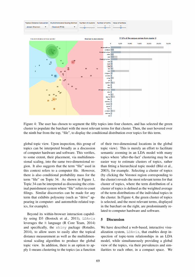
Figure 4: The user has chosen to segment the fifty topics into four clusters, and has selected the greencluster to populate the barchart with the most relevant terms for that cluster. Then, the user hovered overthe ninth bar from the top, “file”, to display the conditional distribution over topics for this term.
global topic view. Upon inspection, this group oftopics can be interpreted broadly as a discussionof computer hardware and software. This verifies,to some extent, their placement, via multidimen-sional scaling, into the same two-dimensional re-gion. It also suggests that the term “file” used inthis context refers to a computer file. However,there is also conditional probability mass for theterm “file” on Topic 34. As shown in Figure 1,Topic 34 can be interpreted as discussing the crim-inal punishment system where “file” refers to courtfilings. Similar discoveries can be made for anyterm that exhibits polysemy (such as “drive” ap-pearing in computer- and automobile-related top-ics, for example).
Beyond its within-browser interaction capabil-ity using D3 (Bostock et al., 2011), LDAvisleverages the R language (R Core Team, 2014)and specifically, the shiny package (Rstudio,2014), to allow users to easily alter the topicaldistance measurement as well as the multidimen-sional scaling algorithm to produce the globaltopic view. In addition, there is an option to ap-ply k-means clustering to the topics (as a function
of their two-dimensional locations in the globaltopic view). This is merely an effort to facilitatesemantic zooming in an LDA model with manytopics where ‘after-the-fact’ clustering may be aneasier way to estimate clusters of topics, ratherthan fitting a hierarchical topic model (Blei et al.,2003), for example. Selecting a cluster of topics(by clicking the Voronoi region corresponding tothe cluster) reveals the most relevant terms for thatcluster of topics, where the term distribution of acluster of topics is defined as the weighted averageof the term distributions of the individual topics inthe cluster. In Figure 4, the green cluster of topicsis selected, and the most relevant terms, displayedin the barchart on the right, are predominantly re-lated to computer hardware and software.
5 Discussion
We have described a web-based, interactive visu-alization system, LDAvis, that enables deep in-spection of topic-term relationships in an LDAmodel, while simultaneously providing a globalview of the topics, via their prevalences and sim-ilarities to each other, in a compact space. We
69
also propose a novel measure, relevance, by whichto rank terms within topics to aid in the taskof topic interpretation, and we present resultsfrom a user study that show that ranking termsin decreasing order of probability is suboptimalfor topic interpretation. The LDAvis visual-ization system (including the user study data) iscurrently available as an R package on GitHub:https://github.com/cpsievert/LDAvis.
For future work, we anticipate performing alarger user study to further understand how to fa-cilitate topic interpretation in fitted LDA mod-els, including a comparison of multiple methods,such as ranking by Turbo Topics (Blei and Laf-ferty, 2009) or FREX scores (Bischof and Airoldi,2012), in addition to relevance. We also note theneed to visualize correlations between topics, asthis can provide insight into what is happening onthe document level without actually displaying en-tire documents. Last, we seek a solution to theproblem of visualizing a large number of topics(say, from 100 - 500 topics) in a compact way.
ReferencesLoulwah AlSumait, Daniel Barbara, James Gentle, and
Carlotta Domeniconi. 2009. Topic SignificanceRanking of LDA Generative Models. ECML.
Jonathan M. Bischof and Edoardo M. Airoldi. 2012.Summarizing topical content with word frequencyand exclusivity. ICML.
David M. Blei, Andrew Y. Ng, and Michael I. Jordan.2012. Latent Dirichlet Allocation. JMLR.
David M. Blei and John Lafferty. 2009. Vi-sualizing Topics with Multi-Word Expressions.arXiv:0907.1013v1 [stat.ML], 2009
David M. Blei, Thomas L. Griffiths, Michael I. Jor-dan, and Joshua B. Tenenbaum. 2003. Hierarchi-cal Topic Models and the Nested Chinese RestaurantProcess. NIPS.
Michael Bostock, Vadim Ogievetsky, Jeffrey Heer2011. D3: Data-Driven Documents. InfoVis.
Allison J.B. Chaney and David M. Blei. 2012. Visual-izing topic models. ICWSM.
Jonathan Chang, Jordan Boyd-Graber, Sean Gerrish,Chong Wang, and David M. Blei. 2009. ReadingTea Leaves: How Humans Interpret Topic Models.NIPS.
Jason Chuang, Daniel Ramage, Christopher D. Man-ning and Jeffrey Heer. 2012a. Interpretation andTrust: Designing Model-Driven Visualizations forText Analysis. CHI.
Jason Chuang, Christopher D. Manning and JeffreyHeer. 2012b. Termite: Visualization Techniques forAssessing Textual Topic Models. AVI.
Jason Chuang, Yuening Hu, Ashley Jin, John D. Wilk-erson, Daniel A. McFarland, Christopher D. Man-ning and Jeffrey Heer. 2013a. Document Explo-ration with Topic Modeling: Designing InteractiveVisualizations to Support Effective Analysis Work-flows. NIPS Workshop on Topic Models: Computa-tion, Application, and Evaluation.
Jason Chuang, Sonal Gupta, Christopher D. Manningand Jeffrey Heer. 2013b. Topic Model Diagnostics:Assessing Domain Relevance via Topical Alignment.ICML.
Matthew J. Gardner, Joshua Lutes, Jeff Lund, JoshHansen, Dan Walker, Eric Ringger, and Kevin Seppi.2010. The topic browser: An interactive tool forbrowsing topic models. NIPS Workshop on Chal-lenges of Data Visualization.
Brynjar Gretarsson, John O’Donovan, Svetlin Bostand-jieb, Tobias Hollerer, Arthur Asuncion, David New-man, and Padhraic Smyth. 2011. TopicNets: VisualAnalysis of Large Text Corpora with Topic Model-ing. ACM Transactions on Intelligent Systems andTechnology, pp 1-26.
Thomas L. Griffiths and Mark Steyvers. 2004. Findingscientific topics. PNAS.
David Mimno, Hanna M. Wallach, Edmund Talley,Miriam Leenders, and Andrew McCallum. 2011.Optimizing Semantic Coherence in Topic Models.EMNLP.
David Newman, Youn Noh, Edmund Talley, SarvnazKarimi, and Timothy Baldwin 2010. EvaluatingTopic Models for Digital Libraries. JCDL.
R Core Team 2014. R: A Language and Envi-ronment for Statistical Computing. http://www.R-project.org.
R Studio, Inc. 2014. shiny: Web Application Frame-work for R; package version 0.9.1. http://CRAN.R-project.org/package=shiny.
Daniel Ramage, Evan Rosen and Jason Chuang andChristopher D. Manning, and Daniel A. McFarland.2009. Topic Modeling for the Social Sciences. NIPSWorkshop on Applications for Topic Models: Textand Beyond.
Justin Snyder, Rebecca Knowles, Mark Dredze,Matthew Gormley, and Travis Wolfe. 2013. TopicModels and Metadata for Visualizing Text Corpora.Proceedings of the 2013 NAACL HLT Demonstra-tion Session.
Matthew A. Taddy 2011. On Estimation and Selectionfor Topic Models. AISTATS.
Hanna M. Wallach, Iain Murray, Ruslan Salakhutdinov,and David Mimno. 2009. Evaluation Methods forTopic Models. ICML.
70
Proceedings of the Workshop on Interactive Language Learning, Visualization, and Interfaces, pages 71–78,Baltimore, Maryland, USA, June 27, 2014. c©2014 Association for Computational Linguistics
Hierarchie: Interactive Visualization for Hierarchical Topic Models
Alison Smith, Timothy Hawes, and Meredith MyersDECISIVE ANALYTICS Corporation
Arlington, VA{alison.smith, timothy.hawes, meredith.myers}@dac.us
Abstract
Existing algorithms for understandinglarge collections of documents often pro-duce output that is nearly as difficultand time consuming to interpret as read-ing each of the documents themselves.Topic modeling is a text understandingalgorithm that discovers the “topics” orthemes within a collection of documents.Tools based on topic modeling become in-creasingly complex as the number of top-ics required to best represent the collec-tion increases. In this work, we presentHierarchie, an interactive visualizationthat adds structure to large topic models,making them approachable and useful toan end user. Additionally, we demonstrateHierarchie’s ability to analyze a diversedocument set regarding a trending newstopic.
1 Introduction
In computational linguistics and related fields, sig-nificant work has been invested in the developmentof algorithms for gaining insight from large bod-ies of text. The raw output of these techniquescan be so complex that it is just as difficult andtime consuming to understand as reading the text.Therefore, it is an especially challenging problemto develop visualizations that add analytic value,making complex analysis accessible by helping auser to understand and interact with the output ofthese algorithms.
Topic Modeling is a common, data-driven tech-nique for summarizing the content of large textcorpora. This technique models documents as dis-tributions of topics and topics as distributions ofwords. In practice, topic models are used to pro-vide a high-level overview and guided explorationof a corpus. Prior work by others (Chaney and
Blei, 2012) and by the author (Smith et al., 2014)has focused on visualizing the results of topicmodeling to support these two goals, but thesevisualizations do not scale beyond 10 to 20 top-ics1. Topic models with a small number of top-ics may not accurately represent very diverse cor-pora; instead, representative topic models requirea number of topics an order of magnitude higher,for which current visualization methods are notsuitable. We propose a visualization that displayshierarchically arranged topics. As opposed to aflat model, which can be thought of as an un-ordered heap of topics, a hierarchical structure al-lows a user to “drill into” topics of interest, mean-ing this technique supports directed exploration ofa corpus regardless of the number of topics in themodel.
Although methods that use inherently hierarchi-cal generative models do exist, we take a simplerecursive approach that scales to large datasets anddoes not change or depend on the underlying topicmodeling implementation. In principle, this tech-nique could be applied to a range of topic model-ing algorithms. We present this hierarchical modelto the user through an intuitive interactive visual-ization, Hierarchie. Additionally, we demonstratethe capability with a Case Study on analyzing thenews coverage surrounding the Malaysia Airlinesflight that went missing on March 8, 2014.
2 Related Work
Latent Dirichlet Allocation (LDA) (Blei et al.,2003b) is an unsupervised algorithm for perform-ing statistical topic modeling that uses a “bag ofwords” approach, treating each document as a setof unordered words. Each document is repre-sented as a probability distribution over some top-ics, and each topic is a probability distribution over
1Either the visualization becomes too confusing to under-stand or using the visualization to explore the corpus takestoo much time — or both.
71
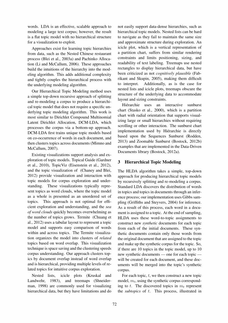
words. LDA is an effective, scalable approach tomodeling a large text corpus; however, the resultis a flat topic model with no hierarchical structurefor a visualization to exploit.
Approaches exist for learning topic hierarchiesfrom data, such as the Nested Chinese restaurantprocess (Blei et al., 2003a) and Pachinko Alloca-tion (Li and McCallum, 2006). These approachesbuild the intuitions of the hierarchy into the mod-eling algorithm. This adds additional complexityand tightly couples the hierarchical process withthe underlying modeling algorithm.
Our Hierarchical Topic Modeling method usesa simple top-down recursive approach of splittingand re-modeling a corpus to produce a hierarchi-cal topic model that does not require a specific un-derlying topic modeling algorithm. This work ismost similar to Dirichlet Compound MultinomialLatent Dirichlet Allocation, DCM-LDA, whichprocesses the corpus via a bottom-up approach.DCM-LDA first trains unique topic models basedon co-occurrence of words in each document, andthen clusters topics across documents (Mimno andMcCallum, 2007).
Existing visualizations support analysis and ex-ploration of topic models. Topical Guide (Gardneret al., 2010), TopicViz (Eisenstein et al., 2012),and the topic visualization of (Chaney and Blei,2012) provide visualization and interaction withtopic models for corpus exploration and under-standing. These visualizations typically repre-sent topics as word clouds, where the topic modelas a whole is presented as an unordered set oftopics. This approach is not optimal for effi-cient exploration and understanding, and the seaof word clouds quickly becomes overwhelming asthe number of topics grows. Termite (Chuang etal., 2012) uses a tabular layout to represent a topicmodel and supports easy comparison of wordswithin and across topics. The Termite visualiza-tion organizes the model into clusters of relatedtopics based on word overlap. This visualizationtechnique is space saving and the clustering speedscorpus understanding. Our approach clusters top-ics by document overlap instead of word overlapand is hierarchical, providing multiple levels of re-lated topics for intuitive corpus exploration.
Nested lists, icicle plots (Kruskal andLandwehr, 1983), and treemaps (Shneider-man, 1998) are commonly used for visualizinghierarchical data, but they have limitations and do
not easily support data-dense hierarchies, such ashierarchical topic models. Nested lists can be hardto navigate as they fail to maintain the same sizeand approximate structure during exploration. Anicicle plot, which is a vertical representation ofa partition chart, suffers from similar renderingconstraints and limits positioning, sizing, andreadability of text labeling. Treemaps use nestedrectangles to display hierarchical data, but havebeen criticized as not cognitively plausible (Fab-rikant and Skupin, 2005), making them difficultto interpret. Additionally, as is the case fornested lists and icicle plots, treemaps obscure thestructure of the underlying data to accommodatelayout and sizing constraints.
Hierarchie uses an interactive sunburstchart (Stasko et al., 2000), which is a partitionchart with radial orientation that supports visual-izing large or small hierarchies without requiringscrolling or other interaction. The sunburst chartimplementation used by Hierarchie is directlybased upon the Sequences Sunburst (Rodden,2013) and Zoomable Sunburst (Bostock, 2012b)examples that are implemented in the Data-DrivenDocuments library (Bostock, 2012a).
3 Hierarchical Topic Modeling
The HLDA algorithm takes a simple, top-downapproach for producing hierarchical topic modelsby recursively splitting and re-modeling a corpus.Standard LDA discovers the distribution of wordsin topics and topics in documents through an infer-ence process; our implementation uses Gibbs sam-pling (Griffiths and Steyvers, 2004) for inference.As a result of this process, each word in a docu-ment is assigned to a topic. At the end of sampling,HLDA uses these word-to-topic assignments toconstruct new synthetic documents for each topicfrom each of the initial documents. These syn-thetic documents contain only those words fromthe original document that are assigned to the topicand make up the synthetic corpus for the topic. So,if there are 10 topics in the topic model, up to 10new synthetic documents — one for each topic —will be created for each document, and these doc-uments will be merged into the topic’s syntheticcorpus.
For each topic, t, we then construct a new topicmodel, mt, using the synthetic corpus correspond-ing to t. The discovered topics in mt representthe subtopics of t. This process, illustrated in
72
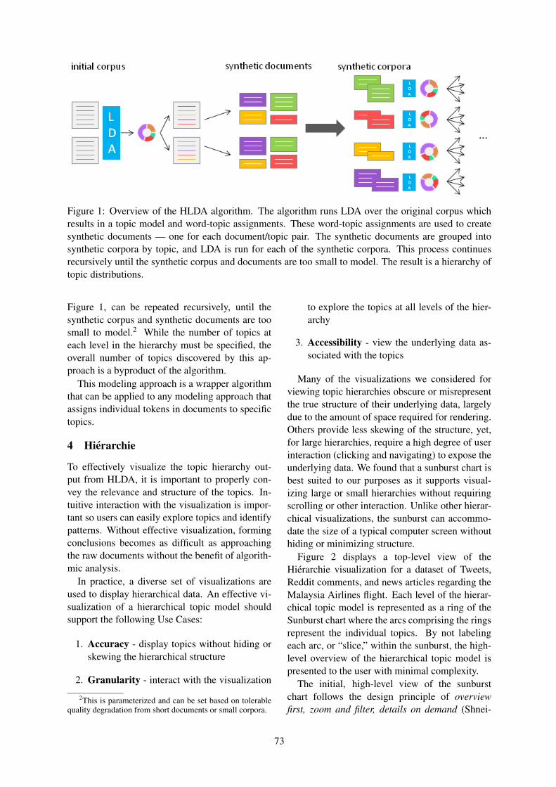
Figure 1: Overview of the HLDA algorithm. The algorithm runs LDA over the original corpus whichresults in a topic model and word-topic assignments. These word-topic assignments are used to createsynthetic documents — one for each document/topic pair. The synthetic documents are grouped intosynthetic corpora by topic, and LDA is run for each of the synthetic corpora. This process continuesrecursively until the synthetic corpus and documents are too small to model. The result is a hierarchy oftopic distributions.
Figure 1, can be repeated recursively, until thesynthetic corpus and synthetic documents are toosmall to model.2 While the number of topics ateach level in the hierarchy must be specified, theoverall number of topics discovered by this ap-proach is a byproduct of the algorithm.
This modeling approach is a wrapper algorithmthat can be applied to any modeling approach thatassigns individual tokens in documents to specifictopics.
4 Hierarchie
To effectively visualize the topic hierarchy out-put from HLDA, it is important to properly con-vey the relevance and structure of the topics. In-tuitive interaction with the visualization is impor-tant so users can easily explore topics and identifypatterns. Without effective visualization, formingconclusions becomes as difficult as approachingthe raw documents without the benefit of algorith-mic analysis.
In practice, a diverse set of visualizations areused to display hierarchical data. An effective vi-sualization of a hierarchical topic model shouldsupport the following Use Cases:
1. Accuracy - display topics without hiding orskewing the hierarchical structure
2. Granularity - interact with the visualization
2This is parameterized and can be set based on tolerablequality degradation from short documents or small corpora.
to explore the topics at all levels of the hier-archy
3. Accessibility - view the underlying data as-sociated with the topics
Many of the visualizations we considered forviewing topic hierarchies obscure or misrepresentthe true structure of their underlying data, largelydue to the amount of space required for rendering.Others provide less skewing of the structure, yet,for large hierarchies, require a high degree of userinteraction (clicking and navigating) to expose theunderlying data. We found that a sunburst chart isbest suited to our purposes as it supports visual-izing large or small hierarchies without requiringscrolling or other interaction. Unlike other hierar-chical visualizations, the sunburst can accommo-date the size of a typical computer screen withouthiding or minimizing structure.
Figure 2 displays a top-level view of theHierarchie visualization for a dataset of Tweets,Reddit comments, and news articles regarding theMalaysia Airlines flight. Each level of the hierar-chical topic model is represented as a ring of theSunburst chart where the arcs comprising the ringsrepresent the individual topics. By not labelingeach arc, or “slice,” within the sunburst, the high-level overview of the hierarchical topic model ispresented to the user with minimal complexity.
The initial, high-level view of the sunburstchart follows the design principle of overviewfirst, zoom and filter, details on demand (Shnei-
73
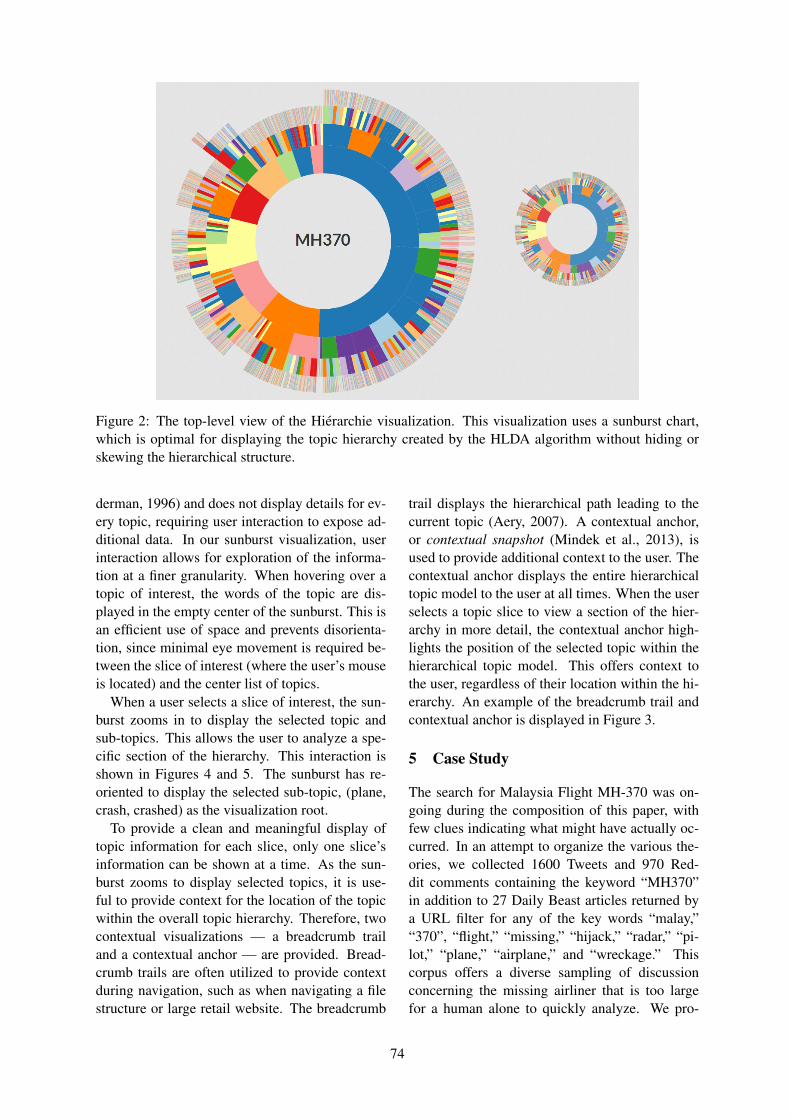
Figure 2: The top-level view of the Hierarchie visualization. This visualization uses a sunburst chart,which is optimal for displaying the topic hierarchy created by the HLDA algorithm without hiding orskewing the hierarchical structure.
derman, 1996) and does not display details for ev-ery topic, requiring user interaction to expose ad-ditional data. In our sunburst visualization, userinteraction allows for exploration of the informa-tion at a finer granularity. When hovering over atopic of interest, the words of the topic are dis-played in the empty center of the sunburst. This isan efficient use of space and prevents disorienta-tion, since minimal eye movement is required be-tween the slice of interest (where the user’s mouseis located) and the center list of topics.
When a user selects a slice of interest, the sun-burst zooms in to display the selected topic andsub-topics. This allows the user to analyze a spe-cific section of the hierarchy. This interaction isshown in Figures 4 and 5. The sunburst has re-oriented to display the selected sub-topic, (plane,crash, crashed) as the visualization root.
To provide a clean and meaningful display oftopic information for each slice, only one slice’sinformation can be shown at a time. As the sun-burst zooms to display selected topics, it is use-ful to provide context for the location of the topicwithin the overall topic hierarchy. Therefore, twocontextual visualizations — a breadcrumb trailand a contextual anchor — are provided. Bread-crumb trails are often utilized to provide contextduring navigation, such as when navigating a filestructure or large retail website. The breadcrumb
trail displays the hierarchical path leading to thecurrent topic (Aery, 2007). A contextual anchor,or contextual snapshot (Mindek et al., 2013), isused to provide additional context to the user. Thecontextual anchor displays the entire hierarchicaltopic model to the user at all times. When the userselects a topic slice to view a section of the hier-archy in more detail, the contextual anchor high-lights the position of the selected topic within thehierarchical topic model. This offers context tothe user, regardless of their location within the hi-erarchy. An example of the breadcrumb trail andcontextual anchor is displayed in Figure 3.
5 Case Study
The search for Malaysia Flight MH-370 was on-going during the composition of this paper, withfew clues indicating what might have actually oc-curred. In an attempt to organize the various the-ories, we collected 1600 Tweets and 970 Red-dit comments containing the keyword “MH370”in addition to 27 Daily Beast articles returned bya URL filter for any of the key words “malay,”“370”, “flight,” “missing,” “hijack,” “radar,” “pi-lot,” “plane,” “airplane,” and “wreckage.” Thiscorpus offers a diverse sampling of discussionconcerning the missing airliner that is too largefor a human alone to quickly analyze. We pro-
74
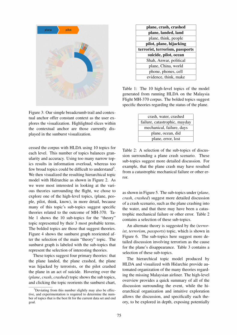
Figure 3: Our simple breadcrumb trail and contex-tual anchor offer constant context as the user ex-plores the visualization. Highlighted slices withinthe contextual anchor are those currently dis-played in the sunburst visualization.
cessed the corpus with HLDA using 10 topics foreach level. This number of topics balances gran-ularity and accuracy. Using too many narrow top-ics results in information overload, whereas toofew broad topics could be difficult to understand3.We then visualized the resulting hierarchical topicmodel with Hierarchie as shown in Figure 2. Aswe were most interested in looking at the vari-ous theories surrounding the flight, we chose toexplore one of the high-level topics, (plane, peo-ple, pilot, think, know), in more detail, becausemany of this topic’s sub-topics suggest specifictheories related to the outcome of MH-370. Ta-ble 1 shows the 10 sub-topics for the “theory”topic represented by their 3 most probable terms.The bolded topics are those that suggest theories.Figure 4 shows the sunburst graph reoriented af-ter the selection of the main “theory” topic. Thesunburst graph is labeled with the sub-topics thatrepresent the selection of interesting theories.
These topics suggest four primary theories: thatthe plane landed, the plane crashed, the planewas hijacked by terrorists, or the pilot crashedthe plane in an act of suicide. Hovering over the(plane, crash, crashed) topic shows the sub topics,and clicking the topic reorients the sunburst chart,
3Deviating from this number slightly may also be effec-tive, and experimentation is required to determine the num-ber of topics that is the best fit for the current data set and endgoal.
plane, crash, crashedplane, landed, landplane, think, people
pilot, plane, hijackingterrorist, terrorism, passports
suicide, pilot, oceanShah, Anwar, political
plane, China, worldphone, phones, cell
evidence, think, make
Table 1: The 10 high-level topics of the modelgenerated from running HLDA on the MalaysiaFlight MH-370 corpus. The bolded topics suggestspecific theories regarding the status of the plane.
crash, water, crashedfailure, catastrophic, mayday
mechanical, failure, daysplane, ocean, didplane, error, lost
Table 2: A selection of the sub-topics of discus-sion surrounding a plane crash scenario. Thesesub-topics suggest more detailed discussion. Forexample, that the plane crash may have resultedfrom a catastrophic mechanical failure or other er-ror.
as shown in Figure 5. The sub-topics under (plane,crash, crashed) suggest more detailed discussionof a crash scenario, such as the plane crashing intothe water, and that there may have been a catas-trophic mechanical failure or other error. Table 2contains a selection of these sub-topics.
An alternate theory is suggested by the (terror-ist, terrorism, passports) topic, which is shown inFigure 6. The sub-topics here suggest more de-tailed discussion involving terrorism as the causefor the plane’s disappearance. Table 3 contains aselection of these sub-topics.
The hierarchical topic model produced byHLDA and visualized with Hiearchie provide au-tomated organization of the many theories regard-ing the missing Malaysian airliner. The high-leveloverview provides a quick summary of all of thediscussion surrounding the event, while the hi-erarchical organization and intuitive explorationallows the discussion, and specifically each the-ory, to be explored in depth, exposing potentially
75
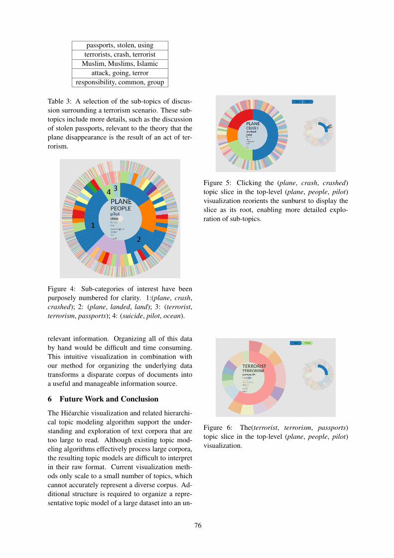
passports, stolen, usingterrorists, crash, terrorist
Muslim, Muslims, Islamicattack, going, terror
responsibility, common, group
Table 3: A selection of the sub-topics of discus-sion surrounding a terrorism scenario. These sub-topics include more details, such as the discussionof stolen passports, relevant to the theory that theplane disappearance is the result of an act of ter-rorism.
Figure 4: Sub-categories of interest have beenpurposely numbered for clarity. 1:(plane, crash,crashed); 2: (plane, landed, land); 3: (terrorist,terrorism, passports); 4: (suicide, pilot, ocean).
relevant information. Organizing all of this databy hand would be difficult and time consuming.This intuitive visualization in combination withour method for organizing the underlying datatransforms a disparate corpus of documents intoa useful and manageable information source.
6 Future Work and Conclusion
The Hiearchie visualization and related hierarchi-cal topic modeling algorithm support the under-standing and exploration of text corpora that aretoo large to read. Although existing topic mod-eling algorithms effectively process large corpora,the resulting topic models are difficult to interpretin their raw format. Current visualization meth-ods only scale to a small number of topics, whichcannot accurately represent a diverse corpus. Ad-ditional structure is required to organize a repre-sentative topic model of a large dataset into an un-
Figure 5: Clicking the (plane, crash, crashed)topic slice in the top-level (plane, people, pilot)visualization reorients the sunburst to display theslice as its root, enabling more detailed explo-ration of sub-topics.
Figure 6: The(terrorist, terrorism, passports)topic slice in the top-level (plane, people, pilot)visualization.
76
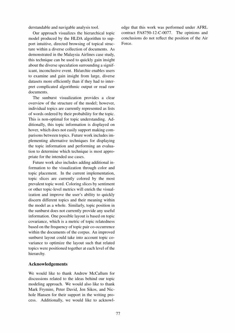
derstandable and navigable analysis tool.Our approach visualizes the hierarchical topic
model produced by the HLDA algorithm to sup-port intuitive, directed browsing of topical struc-ture within a diverse collection of documents. Asdemonstrated in the Malaysia Airlines case study,this technique can be used to quickly gain insightabout the diverse speculation surrounding a signif-icant, inconclusive event. Hiearchie enables usersto examine and gain insight from large, diversedatasets more efficiently than if they had to inter-pret complicated algorithmic output or read rawdocuments.
The sunburst visualization provides a clearoverview of the structure of the model; however,individual topics are currently represented as listsof words ordered by their probability for the topic.This is non-optimal for topic understanding. Ad-ditionally, this topic information is displayed onhover, which does not easily support making com-parisons between topics. Future work includes im-plementing alternative techniques for displayingthe topic information and performing an evalua-tion to determine which technique is most appro-priate for the intended use cases.
Future work also includes adding additional in-formation to the visualization through color andtopic placement. In the current implementation,topic slices are currently colored by the mostprevalent topic word. Coloring slices by sentimentor other topic-level metrics will enrich the visual-ization and improve the user’s ability to quicklydiscern different topics and their meaning withinthe model as a whole. Similarly, topic position inthe sunburst does not currently provide any usefulinformation. One possible layout is based on topiccovariance, which is a metric of topic relatednessbased on the frequency of topic pair co-occurrencewithin the documents of the corpus. An improvedsunburst layout could take into account topic co-variance to optimize the layout such that relatedtopics were positioned together at each level of thehierarchy.
Acknowledgements
We would like to thank Andrew McCallum fordiscussions related to the ideas behind our topicmodeling approach. We would also like to thankMark Frymire, Peter David, Jen Sikos, and Nic-hole Hansen for their support in the writing pro-cess. Additionally, we would like to acknowl-
edge that this work was performed under AFRLcontract FA8750-12-C-0077. The opinions andconclusions do not reflect the position of the AirForce.
77
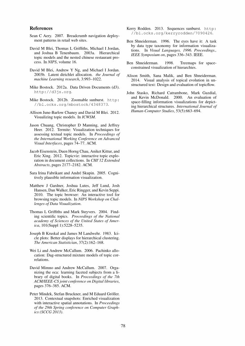
ReferencesSean C Aery. 2007. Breadcrumb navigation deploy-
ment patterns in retail web sites.
David M Blei, Thomas L Griffiths, Michael I Jordan,and Joshua B Tenenbaum. 2003a. Hierarchicaltopic models and the nested chinese restaurant pro-cess. In NIPS, volume 16.
David M Blei, Andrew Y Ng, and Michael I Jordan.2003b. Latent dirichlet allocation. the Journal ofmachine Learning research, 3:993–1022.
Mike Bostock. 2012a. Data Driven Documents (d3).http://d3js.org.
Mike Bostock. 2012b. Zoomable sunburst. http://bl.ocks.org/mbostock/4348373.
Allison June-Barlow Chaney and David M Blei. 2012.Visualizing topic models. In ICWSM.
Jason Chuang, Christopher D Manning, and JeffreyHeer. 2012. Termite: Visualization techniques forassessing textual topic models. In Proceedings ofthe International Working Conference on AdvancedVisual Interfaces, pages 74–77. ACM.
Jacob Eisenstein, Duen Horng Chau, Aniket Kittur, andEric Xing. 2012. Topicviz: interactive topic explo-ration in document collections. In CHI’12 ExtendedAbstracts, pages 2177–2182. ACM.
Sara Irina Fabrikant and Andre Skupin. 2005. Cogni-tively plausible information visualization.
Matthew J Gardner, Joshua Lutes, Jeff Lund, JoshHansen, Dan Walker, Eric Ringger, and Kevin Seppi.2010. The topic browser: An interactive tool forbrowsing topic models. In NIPS Workshop on Chal-lenges of Data Visualization.
Thomas L Griffiths and Mark Steyvers. 2004. Find-ing scientific topics. Proceedings of the Nationalacademy of Sciences of the United States of Amer-ica, 101(Suppl 1):5228–5235.
Joseph B Kruskal and James M Landwehr. 1983. Ici-cle plots: Better displays for hierarchical clustering.The American Statistician, 37(2):162–168.
Wei Li and Andrew McCallum. 2006. Pachinko allo-cation: Dag-structured mixture models of topic cor-relations.
David Mimno and Andrew McCallum. 2007. Orga-nizing the oca: learning faceted subjects from a li-brary of digital books. In Proceedings of the 7thACM/IEEE-CS joint conference on Digital libraries,pages 376–385. ACM.
Peter Mindek, Stefan Bruckner, and M Eduard Groller.2013. Contextual snapshots: Enriched visualizationwith interactive spatial annotations. In Proceedingsof the 29th Spring conference on Computer Graph-ics (SCCG 2013).
Kerry Rodden. 2013. Sequences sunburst. http://bl.ocks.org/kerryrodden/7090426.
Ben Shneiderman. 1996. The eyes have it: A taskby data type taxonomy for information visualiza-tions. In Visual Languages, 1996. Proceedings.,IEEE Symposium on, pages 336–343. IEEE.
Ben Shneiderman. 1998. Treemaps for space-constrained visualization of hierarchies.
Alison Smith, Sana Malik, and Ben Shneiderman.2014. Visual analysis of topical evolution in un-structured text: Design and evaluation of topicflow.
John Stasko, Richard Catrambone, Mark Guzdial,and Kevin McDonald. 2000. An evaluation ofspace-filling information visualizations for depict-ing hierarchical structures. International Journal ofHuman-Computer Studies, 53(5):663–694.
78
Proceedings of the Workshop on Interactive Language Learning, Visualization, and Interfaces, pages 79–82,Baltimore, Maryland, USA, June 27, 2014. c©2014 Association for Computational Linguistics
Concurrent Visualization of Relationships between Words and Topics inTopic Models
Alison Smith∗, Jason Chuang†, Yuening Hu∗, Jordan Boyd-Graber∗, Leah Findlater∗∗University of Maryland, College Park, MD†University of Washington, Seattle, WA
[email protected], [email protected], [email protected], [email protected], [email protected]
Abstract
Analysis tools based on topic models areoften used as a means to explore largeamounts of unstructured data. Users of-ten reason about the correctness of a modelusing relationships between words withinthe topics or topics within the model. Wecompute this useful contextual informa-tion as term co-occurrence and topic co-variance and overlay it on top of stan-dard topic model output via an intuitiveinteractive visualization. This is a workin progress with the end goal to combinethe visual representation with interactionsand online learning, so the users can di-rectly explore (a) why a model may notalign with their intuition and (b) modifythe model as needed.
1 Introduction
Topic modeling is a popular technique for analyz-ing large text corpora. A user is unlikely to havethe time required to understand and exploit the rawresults of topic modeling for analysis of a corpus.Therefore, an interesting and intuitive visualiza-tion is required for a topic model to provide addedvalue. A common topic modeling technique is La-tent Dirichlet Allocation (LDA) (Blei et al., 2003),which is an unsupervised algorithm for perform-ing statistical topic modeling that uses a “bag ofwords” approach. The resulting topic model repre-sents the corpus as an unrelated set of topics whereeach topic is a probability distribution over words.Experienced users who have worked with a textcorpus for an extended period of time often thinkof the thematic relationships in the corpus in termsof higher-level statistics such as (a) inter-topic cor-relations or (b) word correlations. However, stan-dard topic models do not explicitly provide suchcontextual information to the users.
Existing tools based on topic models, suchas Topical Guide (Gardner et al., 2010), Top-icViz (Eisenstein et al., 2012), and the topic vi-sualization of (Chaney and Blei, 2012) supporttopic-based corpus browsing and understanding.Visualizations of this type typically represent stan-dard topic models as a sea of word clouds; the in-dividual topics within the model are presented asan unordered set of word clouds — or somethingsimilar — of the top words for the topic1 whereword size is proportional to the probability of theword for the topic. A primary issue with wordclouds is that they can hinder understanding (Har-ris, 2011) due to the fact that they lack informationabout the relationships between words. Addition-ally, topic model visualizations that display topicsin a random layout can lead to a huge, inefficientlyorganized search space, which is not always help-ful in providing a quick corpus overview or assist-ing the user to diagnose possible problems withthe model.
The authors of Correlated Topic Models (CTM)(Lafferty and Blei, 2006) recognize the limitationof existing topic models to directly model the cor-relation between topics, and present an alterna-tive algorithm, CTM, which models the correla-tion between topics discovered for a corpus by us-ing a more flexible distribution for the topic pro-portions in the model. Topical n-gram models(TNG) (Wang et al., 2007) discover phrases inaddition to topics. TNG is a probabilistic modelwhich assigns words and n-grams based on sur-rounding context, instead of for all references inthe corpus. These models independently accountfor the two limitations of statistical topic modelingdiscussed in this paper by modifying the underly-ing topic modeling algorithm. Our work aims toprovide a low-cost method for incorporating this
1This varies, but typically is either the top 10 to 20 wordsor the number of words which hold a specific portion of thedistribution weight.
79
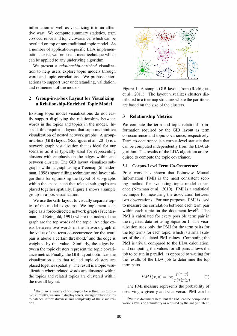
information as well as visualizing it in an effec-tive way. We compute summary statistics, termco-occurrence and topic covariance, which can beoverlaid on top of any traditional topic model. Asa number of application-specific LDA implemen-tations exist, we propose a meta-technique whichcan be applied to any underlying algorithm.
We present a relationship-enriched visualiza-tion to help users explore topic models throughword and topic correlations. We propose inter-actions to support user understanding, validation,and refinement of the models.
2 Group-in-a-box Layout for Visualizinga Relationship-Enriched Topic Model
Existing topic model visualizations do not eas-ily support displaying the relationships betweenwords in the topics and topics in the model. In-stead, this requires a layout that supports intuitivevisualization of nested network graphs. A group-in-a-box (GIB) layout (Rodrigues et al., 2011) is anetwork graph visualization that is ideal for ourscenario as it is typically used for representingclusters with emphasis on the edges within andbetween clusters. The GIB layout visualizes sub-graphs within a graph using a Treemap (Shneider-man, 1998) space filling technique and layout al-gorithms for optimizing the layout of sub-graphswithin the space, such that related sub-graphs areplaced together spatially. Figure 1 shows a samplegroup-in-a-box visualization.
We use the GIB layout to visually separate top-ics of the model as groups. We implement eachtopic as a force-directed network graph (Fruchter-man and Reingold, 1991) where the nodes of thegraph are the top words of the topic. An edge ex-ists between two words in the network graph ifthe value of the term co-occurrence for the wordpair is above a certain threshold,2 and the edge isweighted by this value. Similarly, the edges be-tween the topic clusters represent the topic covari-ance metric. Finally, the GIB layout optimizes thevisualization such that related topic clusters areplaced together spatially. The result is a topic visu-alization where related words are clustered withinthe topics and related topics are clustered withinthe overall layout.
2There are a variety of techniques for setting this thresh-old; currently, we aim to display fewer, stronger relationshipsto balance informativeness and complexity of the visualiza-tion
Figure 1: A sample GIB layout from (Rodrigueset al., 2011). The layout visualizes clusters dis-tributed in a treemap structure where the partitionsare based on the size of the clusters.
3 Relationship Metrics
We compute the term and topic relationship in-formation required by the GIB layout as termco-occurrence and topic covariance, respectively.Term co-occurrence is a corpus-level statistic thatcan be computed independently from the LDA al-gorithm. The results of the LDA algorithm are re-quired to compute the topic covariance.
3.1 Corpus-Level Term Co-OccurrencePrior work has shown that Pointwise MutualInformation (PMI) is the most consistent scor-ing method for evaluating topic model coher-ence (Newman et al., 2010). PMI is a statisticaltechnique for measuring the association betweentwo observations. For our purposes, PMI is usedto measure the correlation between each term pairwithin each topic on the document level3. ThePMI is calculated for every possible term pair inthe ingested data set using Equation 1. The visu-alization uses only the PMI for the term pairs forthe top terms for each topic, which is a small sub-set of the calculated PMI values. Computing thePMI is trivial compared to the LDA calculation,and computing the values for all pairs allows thejob to be run in parallel, as opposed to waiting forthe results of the LDA job to determine the topterm pairs.
PMI(x, y) = logp(x, y)p(x)p(y)
(1)
The PMI measure represents the probability ofobserving x given y and vice-versa. PMI can be
3We use document here, but the PMI can be computed atvarious levels of granularity as required by the analyst intent.
80
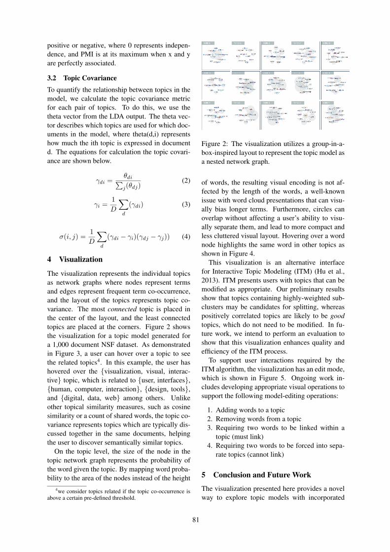
positive or negative, where 0 represents indepen-dence, and PMI is at its maximum when x and yare perfectly associated.
3.2 Topic CovarianceTo quantify the relationship between topics in themodel, we calculate the topic covariance metricfor each pair of topics. To do this, we use thetheta vector from the LDA output. The theta vec-tor describes which topics are used for which doc-uments in the model, where theta(d,i) representshow much the ith topic is expressed in documentd. The equations for calculation the topic covari-ance are shown below.
γdi =θdi∑j(θdj)
(2)
γi =1D
∑d
(γdi) (3)
σ(i, j) =1D
∑d
(γdi − γi)(γdj − γj)) (4)
4 Visualization
The visualization represents the individual topicsas network graphs where nodes represent termsand edges represent frequent term co-occurrence,and the layout of the topics represents topic co-variance. The most connected topic is placed inthe center of the layout, and the least connectedtopics are placed at the corners. Figure 2 showsthe visualization for a topic model generated fora 1,000 document NSF dataset. As demonstratedin Figure 3, a user can hover over a topic to seethe related topics4. In this example, the user hashovered over the {visualization, visual, interac-tive} topic, which is related to {user, interfaces},{human, computer, interaction}, {design, tools},and {digital, data, web} among others. Unlikeother topical similarity measures, such as cosinesimilarity or a count of shared words, the topic co-variance represents topics which are typically dis-cussed together in the same documents, helpingthe user to discover semantically similar topics.
On the topic level, the size of the node in thetopic network graph represents the probability ofthe word given the topic. By mapping word proba-bility to the area of the nodes instead of the height
4we consider topics related if the topic co-occurrence isabove a certain pre-defined threshold.
Figure 2: The visualization utilizes a group-in-a-box-inspired layout to represent the topic model asa nested network graph.
of words, the resulting visual encoding is not af-fected by the length of the words, a well-knownissue with word cloud presentations that can visu-ally bias longer terms. Furthermore, circles canoverlap without affecting a user’s ability to visu-ally separate them, and lead to more compact andless cluttered visual layout. Hovering over a wordnode highlights the same word in other topics asshown in Figure 4.
This visualization is an alternative interfacefor Interactive Topic Modeling (ITM) (Hu et al.,2013). ITM presents users with topics that can bemodified as appropriate. Our preliminary resultsshow that topics containing highly-weighted sub-clusters may be candidates for splitting, whereaspositively correlated topics are likely to be goodtopics, which do not need to be modified. In fu-ture work, we intend to perform an evaluation toshow that this visualization enhances quality andefficiency of the ITM process.
To support user interactions required by theITM algorithm, the visualization has an edit mode,which is shown in Figure 5. Ongoing work in-cludes developing appropriate visual operations tosupport the following model-editing operations:
1. Adding words to a topic2. Removing words from a topic3. Requiring two words to be linked within a
topic (must link)4. Requiring two words to be forced into sepa-
rate topics (cannot link)
5 Conclusion and Future Work
The visualization presented here provides a novelway to explore topic models with incorporated
81
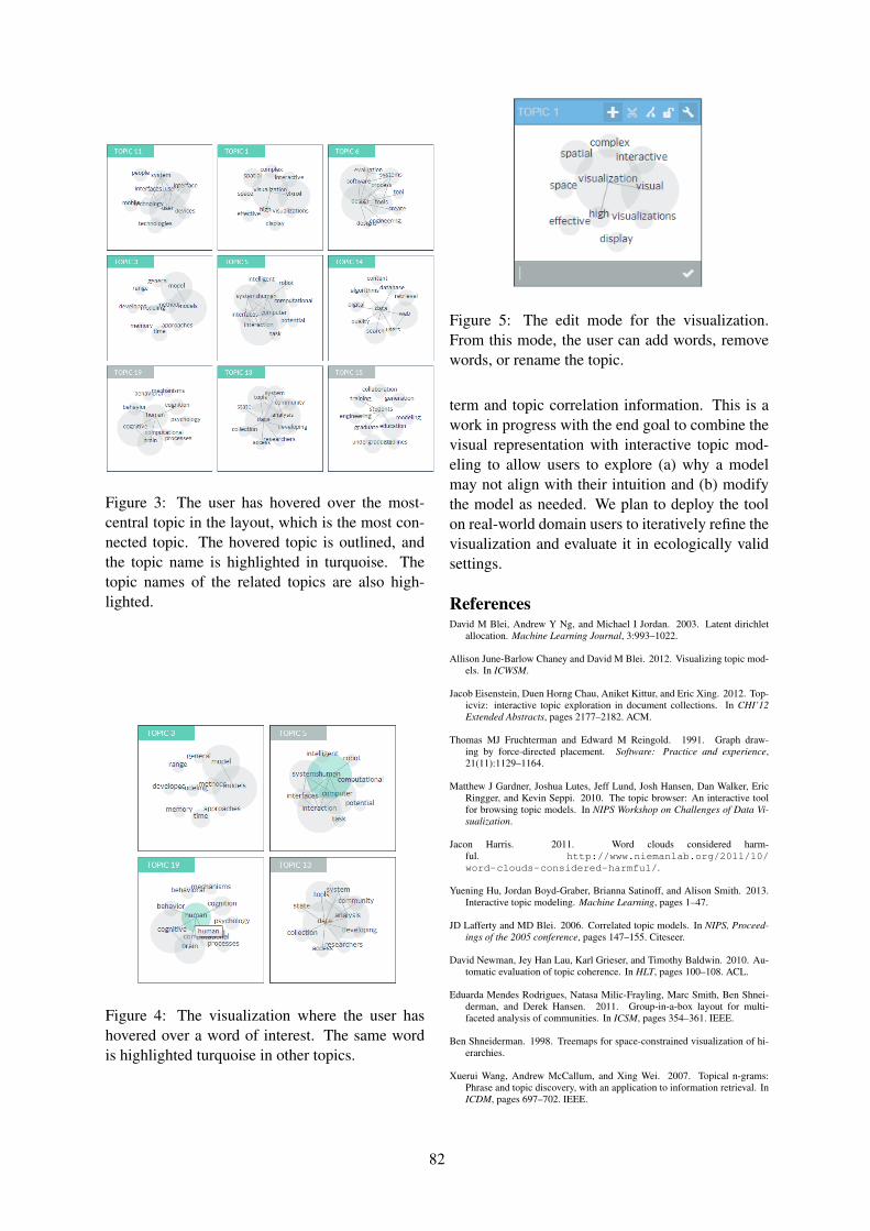
Figure 3: The user has hovered over the most-central topic in the layout, which is the most con-nected topic. The hovered topic is outlined, andthe topic name is highlighted in turquoise. Thetopic names of the related topics are also high-lighted.
Figure 4: The visualization where the user hashovered over a word of interest. The same wordis highlighted turquoise in other topics.
Figure 5: The edit mode for the visualization.From this mode, the user can add words, removewords, or rename the topic.
term and topic correlation information. This is awork in progress with the end goal to combine thevisual representation with interactive topic mod-eling to allow users to explore (a) why a modelmay not align with their intuition and (b) modifythe model as needed. We plan to deploy the toolon real-world domain users to iteratively refine thevisualization and evaluate it in ecologically validsettings.
ReferencesDavid M Blei, Andrew Y Ng, and Michael I Jordan. 2003. Latent dirichlet
allocation. Machine Learning Journal, 3:993–1022.
Allison June-Barlow Chaney and David M Blei. 2012. Visualizing topic mod-els. In ICWSM.
Jacob Eisenstein, Duen Horng Chau, Aniket Kittur, and Eric Xing. 2012. Top-icviz: interactive topic exploration in document collections. In CHI’12Extended Abstracts, pages 2177–2182. ACM.
Thomas MJ Fruchterman and Edward M Reingold. 1991. Graph draw-ing by force-directed placement. Software: Practice and experience,21(11):1129–1164.
Matthew J Gardner, Joshua Lutes, Jeff Lund, Josh Hansen, Dan Walker, EricRingger, and Kevin Seppi. 2010. The topic browser: An interactive toolfor browsing topic models. In NIPS Workshop on Challenges of Data Vi-sualization.
Jacon Harris. 2011. Word clouds considered harm-ful. http://www.niemanlab.org/2011/10/word-clouds-considered-harmful/.
Yuening Hu, Jordan Boyd-Graber, Brianna Satinoff, and Alison Smith. 2013.Interactive topic modeling. Machine Learning, pages 1–47.
JD Lafferty and MD Blei. 2006. Correlated topic models. In NIPS, Proceed-ings of the 2005 conference, pages 147–155. Citeseer.
David Newman, Jey Han Lau, Karl Grieser, and Timothy Baldwin. 2010. Au-tomatic evaluation of topic coherence. In HLT, pages 100–108. ACL.
Eduarda Mendes Rodrigues, Natasa Milic-Frayling, Marc Smith, Ben Shnei-derman, and Derek Hansen. 2011. Group-in-a-box layout for multi-faceted analysis of communities. In ICSM, pages 354–361. IEEE.
Ben Shneiderman. 1998. Treemaps for space-constrained visualization of hi-erarchies.
Xuerui Wang, Andrew McCallum, and Xing Wei. 2007. Topical n-grams:Phrase and topic discovery, with an application to information retrieval. InICDM, pages 697–702. IEEE.
82
Author Index
Boyd-Graber, Jordan, 79
Carenini, Giuseppe, 45Chang, Angel, 14Chen, MeiHua, 34Chiu, Hsun-wen, 34Chuang, Jason, 79Coppersmith, Glen, 22Crowston, Kevin, 59
Downey, Doug, 30
Findlater, Leah, 79
Gupta, Sonal, 38
Hawes, Timothy, 71Hoque, Enamul, 45Hu, Yuening, 79Huang, Shih-Ting, 34
Joty, Shafiq, 45
Kao, Ting-Hui, 34Kelly, Erin, 22
Liew, Jasy Suet Yan, 59
Manning, Christopher, 14, 38McCracken, Nancy, 59Myers, Meredith, 71
O’Connor, Brendan, 1
Pan, Shimei, 30
Savva, Manolis, 14Shirley, Kenneth, 63Sievert, Carson, 63Smith, Alison, 71, 79
Weiss, Rebecca, 53
Yang, Yi, 30Yen, Tzu-Hsi, 34
Zhang, Kunpeng, 30
83


![arXiv:1909.10705v1 [cs.CL] 24 Sep 2019 - nlp.stanford.edu › pubs › see2019massively.pdfStanford University {abisee,apappu,rohun,akhilay,manning}@cs.stanford.edu Abstract Large](https://img.pdfslide.us/doc/110x75/5f1733931d40922a93492bb3/arxiv190910705v1-cscl-24-sep-2019-nlp-a-pubs-a-see2019massivelypdf.jpg)