Embed Size (px)
Citation preview

Proceedings of the First International Workshop
on
ADVANCED ANALYTICS AND LEARNING
ON TEMPORAL DATA
AALTD 2015
Workshop co-located with The European Conference on MachineLearning and Principles and Practice of Knowledge Discovery in
Databases (ECML PKDD 2015)
September 11, 2015. Porto, Portugal
Edited by
Ahlame Douzal-ChouakriaJose A. Vilar
Pierre-Francois MarteauAnn E. Maharaj
Andres M. AlonsoEdoardo Otranto
Irina Nicolae
CEUR Workshop ProceedingsVolume 1425, 2015


Proceedings of
AALTD 2015
First International Workshop on
“Advanced Analytics and Learning
on Temporal Data”
Porto, Portugal
September 11, 2015


Volume Editors
Ahlame Douzal-ChouakriaLIG-AMA, Universite Joseph FourierBatiment Centre Equation 4, Alle de la Palestine a GiresUFR IM2AG, BP 53, F-38041 Grenoble Cedex 9, FranceE:mail: [email protected]
Jose A. Vilar FernandezMODES, Departamento de Matematicas, Universidade da CorunaFacultade de Informatica, Campus de Elvina, s/n, 15071 A Coruna, SpainE:mail: [email protected]
Pierre-Francois MarteauIRISA, ENSIBS, Universite de Bretagne SudCampus de Tohannic, BP 573, 56017 Vannes cedex, FranceE:mail: [email protected]
Ann E. MaharajDepartment of Econometrics and Business Statistics, Monash UniversityCaulfield Campus Building H, Level 5, Room 86900 Dandenong Road, Caulfield East, Victoria 3145, AustraliaE:mail: [email protected]
Andres M. Alonso FernandezDepartamento de Estadıstica, Universidad Carlos III de MadridC/ Madrid, 126, 28903 Getafe (Madrid) SpainE:mail: [email protected]
Edoardo OtrantoDepartment of Cognitive Sciences, Educational and Cultural StudiesUniversity of MessinaVia Concezione, n.6, 98121 Messina, ItalyE:mail: [email protected]
Maria-Irina NicolaeJean Monnet University, Hubert Curien LabE105, 18 rue du Professeur Benoıt Lauras, Saint-Etienne, FranceE:mail: [email protected]
Copyright c⃝ 2015 Douzal, Vilar, Marteau, Maharaj, Alonso, Otranto, Nicolae
Published by the editors on CEUR-WS.ORG
ISSN 1613-0073 Volume 1425 http://CEUR-WS.org/Vol-1425
This volume is published and copyrighted by its editors. The copyright for individualpapers is held by the papers authors. Copying is permitted for private and academicpurposes.
September, 2015


Preface
We are honored to welcome you to the 1st International Workshop on AdvancedAnalytics and Learning on Temporal Data (AALTD), which is held in Porto,Portugal, on September 11th, 2015, co-located with The European Conferenceon Machine Learning and Principles and Practice of Knowledge Discovery inDatabases (ECML PKDD 2015).
The aim of this workshop is to bring together researchers and experts inmachine learning, data mining, pattern analysis and statistics to share theirchallenging issues and advance researches on temporal data analysis. Analysisand learning from temporal data cover a wide scope of tasks including learningmetrics, learning representations, unsupervised feature extraction, clustering andclassification.
This volume contains the conference program, an abstract of the invitedkeynote and the set of regular papers accepted to be presented at the confer-ence. Each of the submitted papers was reviewed by at least two independentreviewers, leading to the selection of seventeen papers accepted for presentationand inclusion into the program and these proceedings. The contributions aregiven by the alphabetical order, by surname. An index of authors can be alsofound at the end of this book.
The keynote given by Gustavo Camps-Valls on “Capturing Time-Structuresin Earth Observation Data with Gaussian Processes” focuses on machine learn-ing models based on Gaussian processes which help to monitor land, oceans, andatmosphere through the estimation of climate and biophysical variables.
The accepted papers spanned from innovative ideas on analytic of temporaldata, including promising new approaches and covering both practical and the-oretical issues. Classification of time series, estimation of graphical models fortemporal data, extraction of patterns from audio streams, searching causal mod-els from longitudinal data and symbolic representation of time series are only asample of the analyzed topics. To introduce the reader, a brief presentation ofthe problems addressed at each of papers is given below.
A novel approach to analyze the evolution of a disease incidence is presentedby Andrade-Pacheco et al. The method is based on Gaussian processes and al-lows to study the effect of the time series components individually and henceto isolate the relevant components and explore short term variations of the dis-ease. Bailly et al introduce a series classification procedure based on extractinglocal features using the Scale-Invariant Feature Transform (SIFT) frameworkand then building a global representation of the series using the Bag-of-Words(BoW) approach. Billard et al propose to highlight the main structure of multi-ple sets of multivariate time series by using principal component analysis wherethe standard correlation structure is replaced by lagged cross-autocorrelation.The symbolic representation of time series SAXO is formalized as a hierarchicalcoclustering approach by Bondu et al, evaluating also its compactness in termsof coding length. A framework to learn an efficient temporal metric by combining
I

several basic metrics for a robust kNN is introduced by Do et al. Dupont andMarteau introduce a sparse version of Dynamic Time Warping (DTW), calledcoarse-DTW, and develop an efficient algorithm (Bubble) to sparse regular timeseries. By coupling both mechanisms, the nearest-neighbor classification of timeseries can be performed much faster.
Gallicchio et al study the balance assessment of elderly people with timeseries acquired with a Wii Balance Board. A novel technique to estimate thewell-known Berg Balance Scale is proposed by using a Reservoir Computingnetwork. Gibberd and Nelson address the estimation of graphical models whendata change over time. Specifically, two extensions of the Gaussian graphicalmodel (GGM) are introduced and empirically examined. Extraction of patternsfrom audio data streams is investigated by Hardy et al considering a symboliza-tion procedure combined with the use of different pattern mining methods. Jainand Spiegel propose a strategy to classify time series consisting of transformingthe series into a dissimilarity representation and then applying PCA followedby an SVM. Krempl addresses the problem of forecasting the density at spatio-temporal coordinates in the future from a sample of pre-fixed instances observedat different positions in the feature space and at different times in the past. Twodifferent approaches using spatio-temporal kernel density estimation are pro-posed. A fuzzy C-medoids algorithm to cluster time series based on comparingestimated quantile autocovariance functions is presented by Lafuente-Rego andVilar.
A new algorithm for discovering causal models from longitudinal data isdeveloped by Rahmadi et al. The method performs structure search over Struc-tural Equation Models (SEMs) by maximizing model scores in terms of data fitand complexity, showing robustness for finite samples. Salperwyck et al intro-duce a clustering technique for time series based on maximizing an inter-inertiacriterion inside parallelized decision trees. An anomaly detection approach fortemporal graph data based on an iterative tensor decomposition and maskingprocedure is presented by Sapienza et al. Soheily-Khah et al perform an exper-imental comparison of several progressive and iterative methods for averagingtime series under dynamic time warping. Finally, Sorokin extends the factoredgated restricted Boltzmann machine model by adding discriminative component,thus enabling it to be used as a classifier and specifically to extract translationalmotion from two related images.
In sum, we think that all these contributions will provide valuable feedbackand motivation to advance research on analysis and learning from temporal data.It is planned that extended versions of the accepted papers will be published ina special volume of Lecture Notes of Artificial Intelligence (LNAI).
We wish to thank the ECML PKDD council members for giving us the op-portunity to hold the AALTD workshop within the framework of the ECMLPKDD Conference and the members of the local organizing committee for theirsupport. Also our gratitude to several colleagues that helped us with the organi-
II

zation of the workshop, particularly Saeid Soheily (Universite Grenoble Alpes,France).
The organizers of the AALTD conference gratefully thank the financial sup-port of the “Programme d’Investissements d’Avenir” of the French governmentthrough the IKATS Project as well as the support received from LIG-AMA,IRISA, MODES, Universite Joseph Fourier and Universidade da Coruna.
Last but not least, we wish to thank the contributing authors for the highquality works and all members of the Reviewing Committee for their invaluableassistance in the selection process. All of them have significantly contributed tothe success of AALTD 2105.
We sincerely hope that the workshop participants have a great and fruitfultime at the conference.
September, 2015 Ahlame Douzal-ChouakriaJose A. Vilar
Pierre-Francois MarteauAnn E. Maharaj
Andres M. AlonsoEdoardo Otranto
Irina Nicolae
III

Program Committee
Ahlame Douzal-Chouakria, Universite Grenoble Alpes, FranceJose Antonio Vilar Fernandez, University of A Coruna, SpainPierre-Francois Marteau, IRISA, Universite de Bretagne-Sud, FranceAnn Maharaj, Monash University, AustraliaAndres M. Alonso, Universidad Carlos III de Madrid, SpainEdoardo Otranto, University of Messina, Italy
Reviewing Committee
Massih-Reza Amini, Universite Grenoble Alpes, FranceManuele Bicego, University of Verona, ItalyGianluca Bontempi, MLG, ULB University, BelgiumAntoine Cornuejols, LRI, AgroParisTech, FrancePierpaolo D’Urso, University La Sapienza, ItalyPatrick Gallinari, LIp. 43, UPMC, FranceEric Gaussier, Universite Grenoble Alpes, FranceChristian Hennig, Department of Statistical Science, London’s Global Univ, UKFrank Hoeppner, Ostfalia University of Applied Sciences, GermanyPaul Honeine, ICD, Universite de Troyes, FranceVincent Lemaire, Orange Lab, FranceManuel Garcıa Magarinos, University of A Coruna, SpainMohamed Nadif, LIPADE, Universite Paris Descartes, FranceFrancois Petitjean, Monash University, AustraliaFabrice Rossi, SAMM, Universite Paris 1, FranceAllan Tucker, Brunel University, UK
IV

Conference programme schedule
Conference venue and some instructions
Within the framework of the ECML PKDD 2015 Conference, the AALTD Work-shop will take place from 15:00 to 18:00 on Friday, September 11, at the AlfandegaCongress Centre, Rua Nova de Alfandega, 4050-430 Porto. The invited talk andthe oral communications will take place at the room Porto, on the second floorof the Congress Centre (see partial site plan below).
The lecture room Porto will be equipped with a PC and a computer projector,which will be used for presentations. Before the session starts, presenters mustprovide to the session chair with the files for the presentation in PDF (Acrobat)or PPT (Powerpoint) format on a USB memory stick. Alternatively, the talkscan be submitted by e-mail to Jose A. Vilar ([email protected]) prior to thestart of the conference. Time planned for each presentation is fifteen minuteswith five additional minutes for discussion.
With regard to the poster session, the authors will be responsible for placingthe posters in the poster panel, which should be carried out well in advance. Themaximum size of the poster is A0.
V

Schedule
Invited talk Chair: Ahlame Douzal
15:00 - 15:30 Capturing Time-Structures in Earth Observation Data with GaussianProcessesGustavo Camps-Valls
Oral communication Chair: Jose A. Vilar
15:30 - 15:50 Time Series Classification in Dissimilarity SpacesBrijnesh J. Jain, Stephan Spiegel
Poster session Chairs: Maria-Irina Nicolae, Saeid Soheily
15:50 - 16:15 See table on next page.
16:00 - 16:15 COFFEE BREAK
Oral communications Chair: Pierre-Francois Marteau
16:15 - 16:35 Fuzzy Clustering of Series Using Quantile AutocovariancesBorja R. Lafuente-Rego, Jose A. Vilar
16:35 - 16:55 Temporal Density ExtrapolationGeorg Krempl
16:55 - 17:15 Coarse-DTW: Exploiting Sparsity in Gesture Time SeriesMarc Dupont, Pierre-Francois Marteau
17:15 - 17:35 Symbolic Representation of Time Series: A Hierarchical CoclusteringFormalizationAlexis Bondu, Marc Boulle, Antoine Cornuejols
17:35 - 17:55 Monitoring Short Term Changes of Malaria Incidence in Uganda withGaussian ProcessesRicardo Andrade Pacheco, Martin Mubangizi, John Quinn, NeilLawrence
VI

Communications in poster session
P1 Bag-of-Temporal-SIFT-Words for Time Series ClassificationAdeline Bailly, Simon Malinowski, Romain Tavenard, ThomasGuyet, Lætitia Chapel
P2 An Exploratory Analysis of Multiple Multivariate Time SeriesLynne Billard, Ahlame Douzal-Chouakria, Seyed Yaser Samadi
P3 Temporal and Frequential Metric Learning for Time Series kNN Clas-sificationCao-Tri Do, Ahlame Douzal-Chouakria, Sylvain Marie, MicheleRombaut
P4 Preliminary Experimental Analysis of Reservoir Computing Ap-proach for Balance AssessmentClaudio Gallicchio, Alessio Micheli, Luca Pedrelli, Federico Vozzi,Oberdan Parodi
P5 Estimating Dynamic Graphical Models fromMultivariate Time-seriesDataAlexander J. Gibberd, James D.B. Nelson
P6 Sequential Pattern Mining on Multimedia DataCorentin Hardy, Laurent Amsaleg, Guillaume Gravier, Simon Mali-nowski, Rene Quiniou
P7 Causality on Longitudinal Data: Stable Specification Search in Con-strained Structural Equation ModelingRidho Rahmadi, Perry Groot, Marianne Heins, Hans Knoop, TomHeskes
P8 CourboSpark: Decision Tree for Time-series on SparkChristophe Salperwyck, Simon Maby, Jerome Cubille, Matthieu La-gacherie
P9 Anomaly Detection in Temporal Graph Data: An Iterative TensorDecomposition and Masking ApproachAnna Sapienza, Andre Panisson, Joseph Wu, Læaetitia Gauvin, CiroCattuto
P10 Progressive and Iterative Approaches for Time Series AveragingSaeid Soheily-Khah, Ahlame Douzal-Chouakria, Eric Gaussier
P11 Classification Factored Gated Restricted Boltzmann MachineIvan Sorokin
VII

VIII

Table of Contents
Capturing Time-structures in Earth Observation Data withGaussian ProcessesG. Camps-Valls . . . . . . . . . . . . . . . . . . . . . . . . . . . . . . . . . . . . . . . . . . . . . . . . 1
Monitoring Short Term Changes of Malaria Incidence inUganda with Gaussian ProcessesR. Andrade-Pacheco, M. Mubangizi, J. Quinn, N. Lawrence . . . . . . . . . 3
Bag-of-Temporal-SIFT-Words for Time Series ClassificationA. Bailly, S. Malinowski, R. Tavenard, T. Guyet, L. Chapel . . . . . . . . . 11
An Exploratory Analysis of Multiple Multivariate Time SeriesL. Billard, A. Douzal-Chouakria, S. Yaser Samadi . . . . . . . . . . . . . . . . . . 19
Symbolic Representation of Time Series: a HierarchicalCoclustering FormalizationA. Bondu, M. Boulle, A. Cornuejols . . . . . . . . . . . . . . . . . . . . . . . . . . . . . . 27
Temporal and Frequential Metric Learning for Time SerieskNN classificationC.-T. Do, A. Douzal-Chouakria, S. Marie, M. Rombaut . . . . . . . . . . . . . 39
Coarse-DTW: Exploiting Sparsity in Gesture Time SeriesM. Dupont, P.-F. Marteau . . . . . . . . . . . . . . . . . . . . . . . . . . . . . . . . . . . . . . 47
Preliminary Experimental Analysis of Reservoir ComputingApproach for Balance AssessmentC. Gallicchio, A. Micheli, L. Pedrelli, F. Vozzi, O. Parodi . . . . . . . . . . . 57
Estimating Dynamic Graphical Models from MultivariateTime-Series DataA.J. Gibberd, J.D.B. Nelson . . . . . . . . . . . . . . . . . . . . . . . . . . . . . . . . . . . . . 63
Sequential Pattern Mining on Multimedia DataC. Hardy, L. Amsaleg, G. Gravier, S. Malinowski, R. Quiniou . . . . . . . . 71
Time Series Classification in Dissimilarity SpacesB.J. Jain, S. Spiegel . . . . . . . . . . . . . . . . . . . . . . . . . . . . . . . . . . . . . . . . . . . . 79
Temporal Density ExtrapolationG. Krempl . . . . . . . . . . . . . . . . . . . . . . . . . . . . . . . . . . . . . . . . . . . . . . . . . . . . 85
Fuzzy Clustering of Series Using Quantile AutocovariancesB. Lafuente-Rego, J.A. Vilar . . . . . . . . . . . . . . . . . . . . . . . . . . . . . . . . . . . . 93
Causality on Longitudinal Data: Stable Specification Searchin Constrained Structural Equation ModelingR. Rahmadi, P. Groot, M. Heins, H. Knoop, T. Heskes . . . . . . . . . . . . . 101
CourboSpark: Decision Tree for Time-series on SparkC Salperwyck, S. Maby, J. Cubille, M. Lagacherie . . . . . . . . . . . . . . . . . . 109
Anomaly Detection in Temporal Graph Data: An IterativeTensor Decomposition and Masking ApproachA. Sapienza, A. Panisson, J. Wu, L. Gauvin, C. Cattuto . . . . . . . . . . . . 117

Table of Contents
Progressive and Iterative Approaches for Time SeriesAveragingS. Soheily-Khah, A. Douzal-Chouakria, E. Gaussier . . . . . . . . . . . . . . . . 123
Classification Factored Gated Restricted Boltzmann MachineI. Sorokin . . . . . . . . . . . . . . . . . . . . . . . . . . . . . . . . . . . . . . . . . . . . . . . . . . . . . 131
X

Proceedings 1st International Workshop on Advanced Analytics and Learning on Temporal DataAALTD 2015
Capturing Time-structures in Earth ObservationData with Gaussian Processes
Gustavo Camps-VallsDepartment of Electrical Engineering, Universitat de Valencia, Spain
Abstract. In this talk I will summarize our experience in the last yearson developing algorithms in the interplay between Physics and Statisti-cal Inference to analyze Earth Observation satellite data. Some of themare currently adopted by ESA and EUMETSAT. I will pay attentionto machine learning models that help to monitor land, oceans, and at-mosphere through the estimation of climate and biophysical variables. Inparticular, I will focus on Gaussian Processes, which provide an adequateframework to design models with high prediction accuracy and able tocope with uncertainties, deal with heteroscedastic noise and particulartime-structures, to encode physical knowledge about the problem, andto attain self-explanatory models. The theoretical developments will beguided by the challenging problems of estimating biophysical parametersat both local and global planetary scales.
Copyright c⃝2015 for this paper by its authors. Copying permitted for private and academicpurposes.
1

2

Proceedings 1st International Workshop on Advanced Analytics and Learning on Temporal DataAALTD 2015
Monitoring Short Term Changes of Malaria
Incidence in Uganda with Gaussian Processes
Ricardo Andrade-Pacheco1, Martin Mubangizi2, John Quinn2,3, and NeilLawrence1
1 University of Sheffield, Department of Computer Science, UK2 Makerere University, College of Computing and Information Science, Uganda
3 UN Global Pulse, Pulse Lab Kampala, Uganda
Abstract. Amethod to monitor communicable diseases based on healthrecords is proposed. The method is applied to health facility records ofmalaria incidence in Uganda. This disease represents a threat for approx-imately 3.3 billion people around the globe. We use Gaussian processeswith vector-valued kernels to analyze time series components individu-ally. This method allows not only removing the effect of specific com-ponents, but studying the components of interest with more detail. Theshort term variations of an infection are divided into four cyclical phases.Under this novel approach, the evolution of a disease incidence can beeasily analyzed and compared between different districts. The graphicaltool provided can help quick response planning and resources allocation.
Keywords: Gaussian processes, malaria, kernel functions, time series.
1 Introduction
More than a century after discovering its transmission mechanism, malaria hasbeen successfully eradicated from different regions of world [15]. However, itis still endemic in 100 countries and represents a threat for 3.3 billion peopleapproximately [20]. In Uganda, malaria is among the leading causes of morbidityand mortality [19]. Different types of interventions can be carried on to preventand treat malaria [20]. Their success depend on how well the disease can beanticipated and how fast the population reacts to it. In this regard, mathematicalmodelling can be a strong ally for decision-making and health services planning.Spatiotemporal modelling for mapping and prediction of infection dynamics is achallenging problem. First of all, because of the costs and difficulties of gatheringdata. Second, because of the challenges of developing a sound theoretical modelthat agrees with the data observed.
The Health Management Information System (HMIS) operated by the UgandaMinistry of Health provides weekly records of the number of patients treated formalaria in different hospitals across the country. Unfortunately, the number ofreporting hospitals is not consistent across time. This variation is prone to createartificial trends in the observed data. Hence, the underreporting effect has to beestimated to be removed.
A common approach for time series analysis is to decompose the observedvariation into specific patterns such as trends, cyclic effects or irregular fluctua-
tions [4, 3, 7]. Gaussian process (GP) models are a natural approach for analyzing
Copyright c©2015 for this paper by its authors. Copying permitted for private and academicpurposes.
3

R. Andrade-Pacheco, M. Mubangizi, J. Quinn, N. Lawrence
functions that represent time series. GPs provide a robust framework for non-parametric probabilistic modelling [18]. The use of covariance kernels enable toanalyse non-linear patterns by embedding an inference problem into an abstractspace with a convenient structure[14]. By combining different covariance kernels(via additions, multiplications or convolutions) into a single one, a GP is able todescribe more complex functions. Each of the individual kernels contributes byencoding a specific set of properties or pattern of the resulting function [5].
We propose a monitoring system for communicable diseases based on Gaus-sian processes. This methodology is able to isolate the relevant components ofthe time series and study the short term variations of the disease. The outputof this system is a graphical tool that discretizes the disease progress into fourphases of simple interpretation.
2 Background
Say we are interested in learning the functional relation, between inputs andoutput, based on a set of observations (xi, yi)
ni=1. GP models introduce an
additional latent variable fx, whose covariance kernel K is a function of theinput values. Usually, yi is considered a distorted version of the latent variable.
To deal with multiple outputs, GP models resort to generalizations of kernelfunctions to the vector-valued case [1]. In time series literature, vector-valuedfunctions are commonly treated in the family of VAR models [12], while in geo-statistics literature co-Kriging generalizations are used [8, 11]. These approachesare equivalent. Let hx = (f1
x, . . . , fd
x)⊤ be a vector-valued GP, its corresponding
covariance matrix is given by
[
cov(hx, hz)ij]
=[
cov(f ix, f j
z)]
. (1)
The diagonal elements of the correlation matrix[
cov(hx, hz)ii]
are just thecovariance functions of the real-valued GP elements. The non-diagonal elementsrepresent the cross-covariance functions between components [9, 10, 2].
3 Method Used
Suppose we have data generated from the combination of two independent sig-nals (see Figure 1a). Usually, not only we are not able to observe the signalsseparately, but the combined signal they yield is corrupted by noise in the datacollected (see Figure 1b). For the sake of this example, suppose that the twosignals of the example represent a long term trend (the smooth signal) and aseasonal component (the sinusoidal signal). For an observer, the oscillations ofthe seasonal component masks the behaviour of the long term trend. At somepoint, however, the observer might want to know whether the trend is increasingor decreasing. Similarly, there might be interest in studying only the seasonal
4

Alarm System for Malaria
component isolated from the trend. For example, in economics and finance, busi-ness recession and expansion periods are determined by studying the cyclic com-ponent of a set of indicators [16]. The cyclic component tells if an indicator isabove or below the trend, and its differences tell if it is increasing or decreasing.
We propose a similar approach for monitoring disease incidence time series,but in our case, we will use a non-parametric approach. To extract the originalsignals, the observed data can be modelled using a GP with a combination ofkernels, say exponentiated quadratics, one having a shorter lengthscale than theother. Figures 1c and 1d shows a model of the combined and independent signals.We also use a vector-valued GP to model directly the derivative of the time series,rather than using simple differences of the observed trend. As a result, we areable to provide uncertainty estimates about the speed of the changes around thetrend. Our approach is based on modelling linear functionals of an underlyingGP [13]. If hx = (fx, ∂fx/∂xi)
⊤, its corresponding kernel is defined as
Γ (xi,xj) =
[
K(xi,xj)∂
∂xjK(xi,xj)
∂∂xi
K(xi,xj)∂2
∂xixjK(xi,xj)
]
. (2)
In most multi-output problems, observations of the different outputs areneeded to learn their relation. Here, the relation between fx and its derivative isknown beforehand through the derivative of K. Thus ∂fx/∂xi can be learnt byrelying entirely on fx. For the signals described above, Figures 1e and 1f showthe corresponding derivatives computed using a kernel of the form of (2). Thederivatives of the long term trend are computed with high confidence, while thederivatives of the seasonal component have more uncertainty. The last is due tothe magnitude of the seasonal component relative to the noise magnitude.
4 Uganda Case
In this exposition we focus on Kabarole district, but provide a snapshot of themonitoring system for all the country. Our base assumption about the infectionprocess of malaria is that it evolves with some degree of smoothness acrosstime. Smooth functions can be represented by a kernel such that the closer theobservations in the input space, the more similar values of the output. TheMatern kernel family satisfies this condition, as it defines dependence throughthe distance between points with some exponential decay [18]. Different membersof this family encode different degrees of smoothness, being the limit case theexponentiated quadratic kernel or RBF, which is infinitely differentiable. Toillustrate our method we will use an RBF kernel. Results with (rougher) Maternkernels do not differ much when used instead.
Despite malaria is a disease influenced by environmental factors like temper-ature or water availability, we could not observe a seasonal effect in HMIS data[6]. If that was the case, the model could be improved incorporating a periodickernel in the covariance structure. Yet, the model fit can be improved if a sec-ond RBF kernel is added. In this case, one kernel has a short lengthscale and
5

6
Alarm System for Malaria
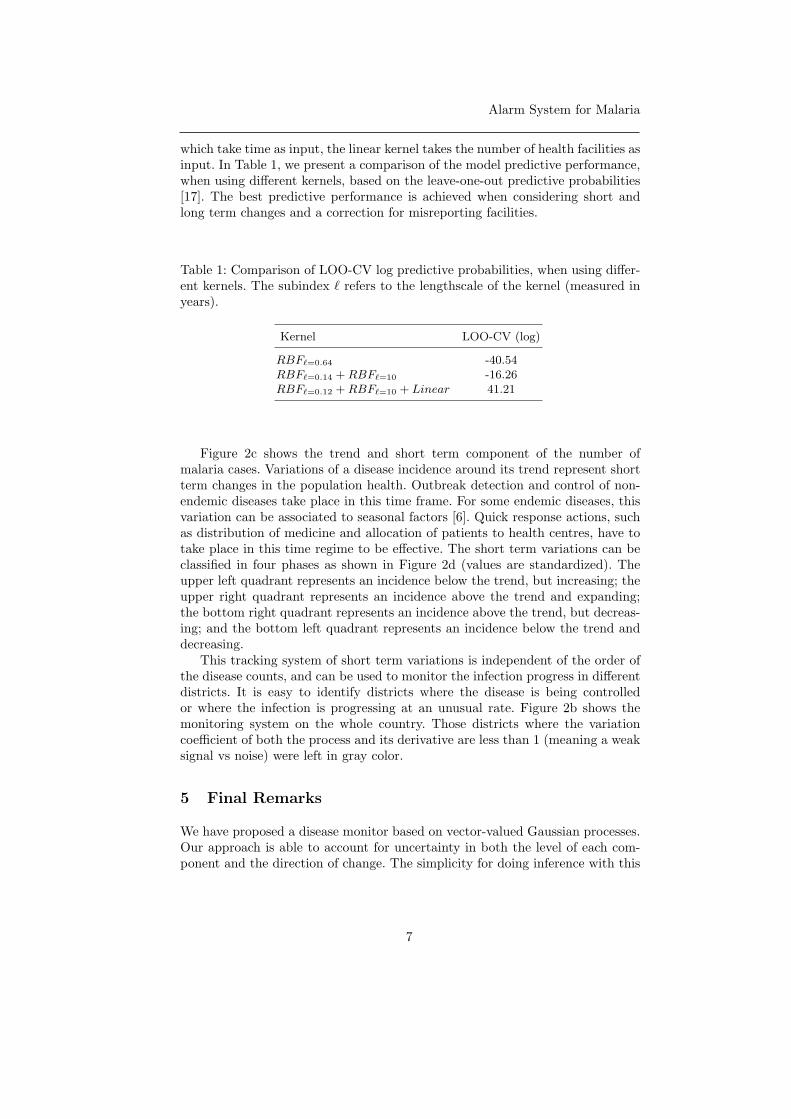
which take time as input, the linear kernel takes the number of health facilities asinput. In Table 1, we present a comparison of the model predictive performance,when using different kernels, based on the leave-one-out predictive probabilities[17]. The best predictive performance is achieved when considering short andlong term changes and a correction for misreporting facilities.
Table 1: Comparison of LOO-CV log predictive probabilities, when using differ-ent kernels. The subindex ℓ refers to the lengthscale of the kernel (measured inyears).
Kernel LOO-CV (log)
RBFℓ=0.64 -40.54RBFℓ=0.14 +RBFℓ=10 -16.26RBFℓ=0.12 +RBFℓ=10 + Linear 41.21
Figure 2c shows the trend and short term component of the number ofmalaria cases. Variations of a disease incidence around its trend represent shortterm changes in the population health. Outbreak detection and control of non-endemic diseases take place in this time frame. For some endemic diseases, thisvariation can be associated to seasonal factors [6]. Quick response actions, suchas distribution of medicine and allocation of patients to health centres, have totake place in this time regime to be effective. The short term variations can beclassified in four phases as shown in Figure 2d (values are standardized). Theupper left quadrant represents an incidence below the trend, but increasing; theupper right quadrant represents an incidence above the trend and expanding;the bottom right quadrant represents an incidence above the trend, but decreas-ing; and the bottom left quadrant represents an incidence below the trend anddecreasing.
This tracking system of short term variations is independent of the order ofthe disease counts, and can be used to monitor the infection progress in differentdistricts. It is easy to identify districts where the disease is being controlledor where the infection is progressing at an unusual rate. Figure 2b shows themonitoring system on the whole country. Those districts where the variationcoefficient of both the process and its derivative are less than 1 (meaning a weaksignal vs noise) were left in gray color.
5 Final Remarks
We have proposed a disease monitor based on vector-valued Gaussian processes.Our approach is able to account for uncertainty in both the level of each com-ponent and the direction of change. The simplicity for doing inference with this
7

8

Alarm System for Malaria
2. L. Baldassarre, L. Rosasco, A. Barla, and A. Verri. Multi-output learning viaspectral filtering. Machine Learning, 87(3):259–301, 2012.
3. M. Baxter and R. G. King. Measuring business cycles: approximate band-passfilters for economic time series. Review of economics and statistics, 81(4):575–593,1999.
4. W. P. Cleveland and G. C. Tiao. Decomposition of seasonal time series: A modelfor the census X-11 program. Journal of the American statistical Association,71(355):581–587, 1976.
5. N. Durrande, J. Hensman, M. Rattray, and N. D. Lawrence. Gaussian processmodels for periodicity detection. arXiv preprint arXiv:1303.7090, 2013.
6. S. I. Hay, R. W. Snow, and D. J. Rogers. From predicting mosquito habitat tomalaria seasons using remotely sensed data: practice, problems and perspectives.Parasitology Today, 14(8):306–313, 1998.
7. A. Hyvarinen and E. Oja. Independent component analysis: algorithms and appli-cations. Neural networks, 13(4):411–430, 2000.
8. G. Matheron. Pour une analyse krigeante de donnes regionalisees. Technical report,Ecole des Mines de Paris, Fontainebleau, France, 1982.
9. C. A. Micchelli and M. Pontil. Kernels for multi-task learning. In Advances inNeural Information Processing Systems (NIPS). MIT Press, 2004.
10. C. A. Micchelli and M. Pontil. On learning vector–valued functions. Neural Com-putation, 17:177–204, 2005.
11. D. E. Myers. Matrix formulation of co-Kriging. Journal of the International As-sociation for Mathematical Geology, 14(3):249–257, 1982.
12. H. Quenouille. The analysis of multiple time-series. Griffin’s statistical monographs& courses. Griffin, 1957.
13. S. Sarkka. Linear operators and stochastic partial differential equations in Gaussianprocess regression. In Artificial Neural Networks and Machine Learning–ICANN2011, pages 151–158. Springer, 2011.
14. J. Shawe-Taylor and N. Cristianini. Kernel Methods for Pattern Analysis. Cam-bridge University Press, Cambridge, U.K., 2004.
15. P. I. Trigg and A. V. Kondrachine. Commentary: malaria control in the 1990s.Bulletin of the World Health Organization, 76(1):11, 1998.
16. F. van Ruth, B. Schouten, and R. Wekker. The statistics Netherlands businesscycle tracer. Methodological aspects; concept, cycle computation and indicatorselection. Technical report, Statistics Netherlands, 2005.
17. A. Vehtari, V. Tolvanen, T. Mononen, and O. Winther. Bayesian leave-one-outcross-validation approximations for Gaussian latent variable models. arXiv preprintarXiv:1412.7461, 2014.
18. C. K. I. Williams and C. E. Rasmussen. Gaussian processes for Machine Learning.MIT Press, 2006.
19. World Health Organization. World health statistics 2015. Technical report, WHOPress, Geneva, 2015.
20. World Health Organization and others. World malaria report 2014. Technicalreport, WHO Press, Geneva, 2014.
9

10

Proceedings 1st International Workshop on Advanced Analytics and Learning on Temporal DataAALTD 2015
Bag-of-Temporal-SIFT-Wordsfor Time Series Classification
Adeline Bailly1, Simon Malinowski2, Romain Tavenard1,Thomas Guyet3, and Lætitia Chapel4
1 Universite de Rennes 2, IRISA, LETG-Rennes COSTEL, Rennes, France2 Universite de Rennes 1, IRISA, Rennes, France
3 Agrocampus Ouest, IRISA, Rennes, France4 Universite de Bretagne Sud, Vannes ; IRISA, Rennes, France
Abstract. Time series classification is an application of particular in-terest with the increase of data to monitor. Classical techniques for timeseries classification rely on point-to-point distances. Recently, Bag-of-Words approaches have been used in this context. Words are quantizedversions of simple features extracted from sliding windows. The SIFTframework has proved efficient for image classification. In this paper, wedesign a time series classification scheme that builds on the SIFT frame-work adapted to time series to feed a Bag-of-Words. Experimental resultsshow competitive performance with respect to classical techniques.
Keywords: time series classification, Bag-of-Words, SIFT, BoTSW
1 Introduction
Classification of time series has received an important amount of interest overthe past years due to many real-life applications, such as environmental mod-eling, speech recognition. A wide range of algorithms have been proposed tosolve this problem. One simple classifier is the k-nearest-neighbor (kNN), whichis usually combined with Euclidean Distance (ED) or Dynamic Time Warping(DTW) [11]. Such techniques compute similarity between time series based onpoint-to-point comparisons, which is often not appropriate. Classification tech-niques based on higher level structures are most of the time faster, while beingat least as accurate as DTW-based classifiers. Hence, various works have inves-tigated the extraction of local and global features in time series. Among theseworks, the Bag-of-Words (BoW) approach (also called bag-of-features) has beenconsidered for time series classification. BoW is a very common technique intext mining, information retrieval and content-based image retrieval because ofits simplicity and performance. For these reasons, it has been adapted to timeseries data in some recent works [1, 2, 9, 12, 14]. Different kinds of features basedon simple statistics have been used to create the words.
In the context of image retrieval and classification, scale-invariant descriptorshave proved their efficiency. Particularly, the Scale-Invariant Feature Transform(SIFT) framework has led to widely used descriptors [10]. These descriptorsare scale and rotation invariant while being robust to noise. We build on thisframework to design a BoW approach for time series classification where the
Copyright c©2015 for this paper by its authors. Copying permitted for private and academicpurposes.
11

A. Bailly, S. Malinowski, R. Tavenard, T. Guyet, L.Chapel
words correspond to the description of local gradients around keypoints, that arefirst extracted from the time series. This approach can be seen as an adaptationof the SIFT framework to time series.
This paper is organized as follows. Section 2 summarizes related work, Sec-tion 3 describes the proposed Bag-of-Temporal-SIFT-Words (BoTSW) method,and Section 4 reports experimental results. Finally, Section 5 concludes anddiscusses future work.
2 Related work
Our approach for time series classification builds on two well-known methodsin computer vision: local features are extracted from time series using a SIFT-based approach and a global representation of time series is built using Bag-of-Words. This section first introduces state-of-the-art methods in time seriesclassification, then presents standard approaches for extracting features in theimage classification context and finally lists previous works that make use ofsuch approaches for time series classification.
Data mining community has, for long, investigated the field of time seriesclassification. Early works focus on the use of dedicated metrics to assess sim-ilarity between time series. In [11], Ratanamahatana and Keogh compare Dy-namic Time Warping to Euclidean Distance when used with a simple kNN clas-sifier. While the former benefits from its robustness to temporal distortions toachieve high efficiency, ED is known to have much lower computational cost.Cuturi [4] shows that DTW fails at precisely quantifying dissimilarity betweennon-matching sequences. He introduces Global Alignment Kernel that takes intoaccount all possible alignments to produce a reliable dissimilarity metric to beused with kernel methods such as Support Vector Machines (SVM). Douzal andAmblard [5] investigate the use of time series metrics for classification trees.
So as to efficiently classify images, those first have to be described accurately.Both local and global descriptions have been proposed by the computer visioncommunity. For long, the most powerful local feature for images was SIFT [10]that describes detected keypoints in the image using the gradients in the regionssurrounding those points. Building on this, Sivic and Zisserman [13] suggestedto compare video frames using standard text mining approaches in which docu-ments are represented by word histograms, known as Bag-of-Words (BoW). Todo so, authors map the 128-dimensional space of SIFT features to a codebookof few thousand words using vector quantization. VLAD (Vector of Locally Ag-gregated Descriptors) [6] are global features that build upon local ones in thesame spirit as BoW. Instead of storing counts for each word in the dictionary,VLAD preserves residuals to build a fine-grain global representation.
Inspired by text mining, information retrieval and computer vision commu-nities, recent works have investigated the use of Bag-of-Words for time seriesclassification [1, 2, 9, 12, 14]. These works are based on two main operations: con-verting time series into Bag-of-Words (a histogram representing the occurrenceof words), and building a classifier upon this BoW representation. Usually, clas-
12

Bag-of-Temporal-SIFT-Words for Time Series Classification
sical techniques are used for the classification step: random forests, SVM, neuralnetworks, kNN. In the following, we focus on explaining how the conversion oftime series into BoW is performed in the literature. In [2], local features such asmean, variance, extremum values are computed on sliding windows. These fea-tures are then quantized into words using a codebook learned by a class proba-bility estimate distribution. In [14], discrete wavelet coefficients are extracted onsliding windows and then quantized into words using k-means. In [9, 12], wordsare constructed using the SAX representation [8] of time series. SAX symbolsare extracted from time series and histograms of n-grams of these symbols arecomputed. In [1], multivariate time series are transformed into a feature matrix,whose rows are feature vectors containing a time index, the values and the gradi-ent of time series at this time index (on all dimensions). Random samples of thismatrix are given to decision trees whose leaves are seen as words. A histogramof words is output when the different trees are learned. Rather than computingfeatures on sliding windows, authors of [15] first extract keypoints from timeseries. These keypoints are selected using the Differences-of-Gaussians (DoG)framework, well-known in the image community, that can be adapted to one-dimensional signals. Keypoints are then described by scale-invariant featuresthat describe the shapes of the extremum surrounding keypoints. In [3], extrac-tion and description of time series keypoints in a SIFT-like framework is usedto reduce the complexity of Dynamic Time Warping: features are used to matchanchor points from two different time series and prune the search space whenfinding the optimal path in the DTW computation.
In this paper, we design a time series classification technique based on theextraction and the description of keypoints using a SIFT framework adapted totime series. The description of keypoints is quantized using a k-means algorithmto create a codebook of words and classification of time series is performed witha linear SVM fed with normalized histograms of words.
3 Bag-of-Temporal-SIFT-Words (BoTSW) method
The proposed method is adapted from the SIFT framework [10] widely used forimage classification. It is based on three main steps : (i) detection of keypoints(scale-space extrema) in time series, (ii) description of these keypoints by gra-dient magnitude at a specific scale, and (iii) representation of time series by aBoW, words corresponding to quantized version of the description of keypoints.These steps are depicted in Fig. 1 and detailed below.
Following the SIFT framework, keypoints in time series correspond to localextrema both in terms of scale and location. These scale-space extrema are iden-tified using a DoG function, which establishes a list of scale-invariant keypoints.Let L(t, σ) be the convolution (∗) of a Gaussian function G(t, σ) of width σ witha time series S(t):
L(t, σ) = G(t, σ) ∗ S(t).
DoG is obtained by subtracting two time series filtered at consecutive scales:
D(t, σ) = L(t, kscσ)− L(t, σ),
13

14

Bag-of-Temporal-SIFT-Words for Time Series Classification
DatasetBoTSW +linear SVM
BoTSW +1NN
ED +1NN
DTW +1NN
k nb ER k nb ER ER ER
50words 512 16 0.363 1024 16 0.400 0.369 0.310
Adiac 512 16 0.614 128 16 0.642 0.389 0.396Beef 128 10 0.400 128 16 0.300 0.467 0.500CBF 64 6 0.058 64 14 0.049 0.148 0.003
Coffee 256 4 0.000 64 12 0.000 0.250 0.179ECG200 256 16 0.110 64 12 0.160 0.120 0.230Face (all) 1024 8 0.218 512 16 0.239 0.286 0.192
Face (four) 128 12 0.000 128 6 0.046 0.216 0.170Fish 512 16 0.069 512 14 0.149 0.217 0.167
Gun-Point 256 4 0.080 256 10 0.067 0.087 0.093Lightning-2 16 16 0.361 512 16 0.410 0.246 0.131
Lightning-7 512 14 0.384 512 14 0.480 0.425 0.274
Olive Oil 256 4 0.100 512 2 0.100 0.133 0.133OSU Leaf 1024 10 0.182 1024 16 0.248 0.483 0.409
Swedish Leaf 1024 16 0.152 512 10 0.229 0.213 0.210Synthetic Control 512 14 0.043 64 8 0.093 0.120 0.007
Trace 128 10 0.010 64 12 0.000 0.240 0.000
Two Patterns 1024 16 0.002 1024 16 0.009 0.090 0.000
Wafer 512 12 0.001 512 12 0.001 0.005 0.020Yoga 1024 16 0.150 512 6 0.230 0.170 0.164
Table 1: Classification error rates (best performance is written as bold text).
frequency vector) of word occurrences. These histograms are then passed to aclassifier to learn how to discriminate classes from this BoTSW description.
4 Experiments and results
In this section, we investigate the impact of both the number of blocks nb and thenumber of words k in the codebook (defined in Section 3) on classification errorrates. Experiments are conducted on 20 datasets from the UCR repository [7].We set all parameters of BoTSW but nb and k as follows : σ = 1.6, ksc = 21/3,a = 8. These values have shown to produce stable results. Parameters nb andk vary inside the following sets : 2, 4, 6, 8, 10, 12, 14, 16 and
2i, ∀ i ∈ 2..10
respectively. Codebooks are obtained via k-means quantization. Two classifiersare used to classify times series represented as BoTSW : a linear SVM or a 1NNclassifier. Each dataset is composed of a train and a test set. For our approach,the best set of (k, nb) parameters is selected by performing a leave-one-out cross-validation on the train set. This best set of parameters is then used to build theclassifier on the train set and evaluate it on the test set. Experimental error rates(ER) are reported in Table 1, together with baseline scores publicly availableat [7].
15

A. Bailly, S. Malinowski, R. Tavenard, T. Guyet, L.Chapel
0
0.1
0.2
0.3
0.4
0.5
4 16 64 256 1024
Error r
ate
Number of codewords
nb = 4
nb = 10
nb = 16
0
0.1
0.2
0.3
0.4
0.5
2 4 6 8 10 12 14 16
Error r
ate
Number of SIFT bins
k = 64
k = 256
k = 1024
Fig. 2: Classification accuracy on dataset Yoga as a function of k and nb.
ED+1NN
DTW+1NN
TSBF[2]SAX-
VSM[12]SMTS[1] BoP[9]
W T L W T L W T L W T L W T L W T L
BoTSW+lin. SVM 18 0 2 11 0 9 8 0 12 9 2 9 7 0 13 14 0 6
BoTSW + 1NN 13 0 7 9 1 10 5 0 15 4 3 13 4 1 15 7 1 12
Table 2: Win-Tie-Lose (WTL) scores comparing BoTSW to state-of-the-artmethods. For instance, BoTSW+linear SVM reaches better performance thanED+1NN on 18 datasets, and worse performance on 2 datasets.
BoTSW coupled with a linear SVM is better than both ED and DTW on11 datasets. It is also better than BoTSW coupled with a 1NN classifier on13 datasets. We also compared our approach with classical techniques for timeseries classification. We varied number of codewords k between 4 and 1024. Notsurprisingly, cross-validation tends to select large codebooks that lead to moreprecise representation of time series by BoTSW. Fig. 2 shows undoubtedly that,for Yoga dataset, (left) the larger the codebook, the better the results and (right)the choice of the number nb of blocks is less crucial as a wide range of valuesyield competitive classification performance.
Win-Tie-Lose scores (see Table 2) show that coupling BoTSW with a linearSVM reaches competitive performance with respect to the literature.
As it can be seen in Table 1, BoTSW is (by far) less efficient than both EDand DTW for dataset Adiac. As BoW representation maps keypoint descriptionsinto words, details are lost during this quantization step. Knowing that only veryfew keypoints are detected for these Adiac time series, we believe a more preciserepresentation would help.
5 Conclusion
BoTSW transforms time series into histograms of quantized local features. Dis-tinctiveness of the SIFT keypoints used with Bag-of-Words enables to efficientlyand accurately classify time series, despite the fact that BoW representation
16

Bag-of-Temporal-SIFT-Words for Time Series Classification
ignores temporal order. We believe classification performance could be furtherimproved by taking time information into account and/or reducing the impactof quantization losses in our representation.
Acknowledgments
This work has been partly funded by ANR project ASTERIX (ANR-13-JS02-0005-01), Region Bretagne and CNES-TOSCA project VEGIDAR.
References
1. M. G. Baydogan and G. Runger. Learning a symbolic representation for multi-variate time series classification. DMKD, 29(2):400–422, 2015.
2. M. G. Baydogan, G. Runger, and E. Tuv. A Bag-of-Features Framework to ClassifyTime Series. IEEE PAMI, 35(11):2796–2802, 2013.
3. K. S. Candan, R. Rossini, and M. L. Sapino. sDTW: Computing DTW Distancesusing Locally Relevant Constraints based on Salient Feature Alignments. Proc.
VLDB, 5(11):1519–1530, 2012.4. M. Cuturi. Fast global alignment kernels. In Proc. ICML, pages 929–936, 2011.5. A. Douzal-Chouakria and C. Amblard. Classification trees for time series. Elsevier
Pattern Recognition, 45(3):1076–1091, 2012.6. H. Jegou, M. Douze, C. Schmid, and P. Perez. Aggregating local descriptors into
a compact image representation. In Proc. CVPR, pages 3304–3311, 2010.7. E. Keogh, Q. Zhu, B. Hu, Y. Hao, X. Xi, L. Wei, and C. A. Ratanama-
hatana. The UCR Time Series Classification/Clustering Homepage, 2011.www.cs.ucr.edu/~eamonn/time_series_data/.
8. J. Lin, E. Keogh, S. Lonardi, and B. Chiu. A symbolic representation of time series,with implications for streaming algorithms. In Proc. ACM SIGMOD Workshop on
Research Issues in DMKD, pages 2–11, 2003.9. J. Lin, R. Khade, and Y. Li. Rotation-invariant similarity in time series using
bag-of-patterns representation. IJIS, 39:287–315, 2012.10. D. G. Lowe. Distinctive image features from scale-invariant keypoints. IJCV,
60(2):91–110, 2004.11. C. A. Ratanamahatana and E. Keogh. Everything you know about dynamic time
warping is wrong. In Proc. ACM SIGKDD Workshop on Mining Temporal and
Sequential Data, pages 22–25, 2004.12. P. Senin and S. Malinchik. SAX-VSM: Interpretable Time Series Classification
Using SAX and Vector Space Model. Proc. ICDM, pages 1175–1180, 2013.13. J. Sivic and A. Zisserman. Video Google: A text retrieval approach to object
matching in videos. In Proc. ICCV, pages 1470–1477, 2003.14. J. Wang, P. Liu, M. F.H. She, S. Nahavandi, and A. Kouzani. Bag-of-words Rep-
resentation for Biomedical Time Series Classification. BSPC, 8(6):634–644, 2013.15. J. Xie and M. Beigi. A Scale-Invariant Local Descriptor for Event Recognition in
1D Sensor Signals. In Proc. ICME, pages 1226–1229, 2009.
17

18

Proceedings 1st International Workshop on Advanced Analytics and Learning on Temporal DataAALTD 2015
An Exploratory Analysis of Multiple
Multivariate Time Series
Lynne Billard1, Ahlame Douzal-Chouakria2, and Seyed Yaser Samadi3
1 Department of Statistics, University of Georgia2 Universite Grenoble Alpes, CNRS - LIG/AMA, France
3 Department of Mathematics, Southern Illinois University
Abstract. Our aim is to extend standard principal component analysis
for non-time series data to explore and highlight the main structure of
multiple sets of multivariate time series. To this end, standard variance-
covariance matrices are generalized to lagged cross-autocorrelation ma-
trices. The methodology produces principal component time series, which
can be analysed in the usual way on a principal component plot, except
that the plot also includes time as an additional dimension.
1 Introduction
Time series data are ubiquitous, arising throughout economics, meteorology,
medicine, the basic sciences, even in some genetic microarrays, to name a few of
the myriad fields of application. Multivariate time series are likewise prevalent.
Our aim is to use principal components methods as an exploratory technique to
find clusters of time series in a set of S multivariate time series. For example,
in a collection of stock market time series, interest may center on whether some
stocks, such as mining stocks, behave alike but differently from other stocks,
such as pharmaceutical stocks.
A seminal paper in univariate time series clustering is that of Kosmelj and
Batagelj (1990), based on a dissimilarity measure. Since then several researchers
have proposed other approaches (e.g. Caiado et al (2015), D’Urso and Maharaj
(2009)). A comprehensive summary of clustering for univariate time series is in
Liao (2005). Liao (2007) introduced a two-step procedure for multivariate series
which transformed the observations into a single multivariate series. Most of
these methods use dissimilarity functions or variations thereof. A summary of
Liao (2005, 2007) along with more recent proposed methods is in Billard et al.
(2015). Though a few authors specify a particular model structure, by and large,
the dependence information inherent to time series observations is not used.
Dependencies in time series are measured through the autocorrelation (or,
equivalently, the autocovariance) functions. In this work, we illustrate how these
Copyright c⃝2015 for this paper by its authors. Copying permitted for private and academicpurposes.
19

L. Billard, A. Douzal-Chouakria, S. Yaser Samadi
dependencies can be used in a principal component analysis. This produces prin-
cipal component time series, which in turn allows the projection of the original
time series observations onto three dimensional principal component by time
space. The basic methodology is outlined in Section2, and illustrated in Section
3.
2 Methodology
2.1 Cross-Autocorrelation functions for S > 1 series and p > 1
dimensions
Let Xst = (Xstj), j = 1, . . . , p, t = 1, . . . , Ns, s = 1, . . . , S, be a p-dimensional
time series of length Ns, for each series s. For notational simplicity, assume
Ns = N for all s. Let us also assume the observations have been suitably differ-
enced/transformed so that the data are stationary.
For a standard single univariate series time series where S = 1 and p = 1, it
is well-known that the sample autocovariance function at lag k is (dropping the
s = S = 1 and j = p = 1 subscripts)
γ(k) =1
N
N−k∑t=1
(Xt − X)(Xt+k − X), k = 0, 1, . . . , X =1
N
N∑t=1
Xt, (2.1)
and the sample autocorrelation function at lag k is ρ(k) = γ(k)/γ(0), k =
0, 1, . . ..
These autocorrelation functions provide a measure of the time dependence
between observations changes as their distance apart, lag k. They are used to
identify the type of model and also to estimate model parameters. See, many
of the basic texts on time series, e.g., Box et al. (2011); Brockwell and Davis
(1991); Cryer and Chan (2008). Note that the divisor in Eq.(2.1) is N , rather
than N −k. This ensures that the sample autocovariance matrix is non-negative
definite.
For a single multivariate time series where S = 1 and p ≥ 1, the cross-
autocovariance function between variables (j, j′) at lag k is the p × p matrix
Γ (k) with elements estimated by
γjj′(k) =1
T
T−k∑t=1
(Xtj − Xj)(Xt+k,j′ − Xj′), k = 0, 1,with Xj =1
N
N∑t=1
Xtj ,
(2.2)
20

An Exploratory Analysis of Multiple Multivariate Time Series
and the cross-autocorrelation function between variables (j, j′) at lag k is the
p× p matrix, ρ(k), with elements ρjj′(k), j, j′ = 1, . . . , p estimated by
ρjj′(k) = γjj′(k)/γjj(0)γj′j′(0)1/2, k = 0, 1, . . . . (2.3)
Unlike the autocorrelation function obtained from Eq.(2.1) with its single
value at each lag k, Eq.(2.3) produces a p×p matrix at each lag k. The function
Eq.(2.2) was first given by Whittle (1963) and shown to be nonsymmetric by
Jones (1964). In general, ρjj′(k) = ρj′j(k) for variables j = j′, except for k = 0,
but ρ(k) = ρ′(−k); see, e.g., Brockwell and Davis (1991).
When there are S ≥ 1 series and p ≥ 1 variables, the definition of Eqs.(2.2)-
(2.3) can be extended to give a p×p sample cross-autocovariance function matrix
between variables (j, j′) at lag k, Γ (k), with elements given by, for j, j′ =
1, . . . , p,
γjj′(k) =1
NS
S∑s=1
N−k∑t=1
(Xstj − Xj)(Xs,t+k,j′ − Xj′), k = 0, 1, (2.4)
with Xj =1
NS
S∑s=1
N∑t=1
Xstj ;
and the p × p sample cross-autocorrelation matrix at lag k, ρ(1)(k), has ele-
ments ρjj′(k), j, j′ = 1, . . . , p, obtained by substituting Eq.(2.4) into Eq.(2.3).
This cross-autocovariance function in Eq.(2.4) is a measure of time dependence
between observations k units apart for a given variable pair (j, j′), calculated
across all S series. Notice, the sample means Xj in Eq.(2.4) are calculated across
all NS observations.
An alternative approach is to calculate these sample means by series. In
this case, the cross-autocovariance matrix Γ (k) has elements estimated by, for
j, j′ = 1, . . . , p, s = 1, . . . , S,
γjj′(k) =1
NS
S∑s=1
N−k∑t=1
(Xstj − Xsj)(Xs,t+k,j − Xsj′), k = 0, 1, (2.5)
with Xsj =1
N
N∑t=1
Xstj ;
and the corresponding p × p cross-autocorrelation function matrix ρ(2)(k) has
elements ρjj′(k) found by substituting Eq.(2.5) into Eq.(2.3).
Other model structures can be considered, which would provide other options
for obtaining the relevant sample means. These include class structures, lag k
structures, weighted series and/or weighted variable structures, and the like; see
Billard et al. (2015).
21
L. Billard, A. Douzal-Chouakria, S. Yaser Samadi
2.2 Principal Components for Time Series
In a standard classical principal component analysis on a set of p-dimensional
multivariate observations X = Xij , i = 1, . . . n, j = 1, . . . , p, each observation
is projected into a corresponding νth order principal component, PCν(i), through
the linear combination of the observation’s variables,
PCν(i) = wν1Xi1 + · · ·+ wνpXip, ν = 1, . . . , p, (2.6)
where wν = (wν1, . . . , wνp) is the νth eigenvector of the correlation matrix ρ (or,
equivalently for non-standardized observations, the variance-covariance matrix
Σ). The eigenvalues satisfy λ1 ≥ λ2 ≥ . . . ≥ λp ≥ 0, and∑p
ν=1 λν = p (or, σ2 for
non-standardized data). A detailed description of this methodology for standard
data can be found in any of the numerous texts on multivariate analysis, e.g.,
Joliffe (1986) and Johnson and Wichern (2007) for an applied approach, and
Anderson (1984) for theoretical details.
For time series data, the correlation matrix ρ is replaced by the cross-
autocorrelation matrix ρ(k), for a specific lag k = 1, 2, . . . , and the νth order
principal component of Eq.(2.6) becomes
PCν(s, t) = wν1Xs1t + · · ·+wνpXspt, ν = 1, . . . , p, t = 1, . . . , N, s = 1, . . . , S.
(2.7)
The elements of ρ(k) can be estimated by ρjj′(k) from Eq.(2.4) or from Eq.(2.5)
(or from other choices of model structure). The problem of non-positive defi-
niteness, for lag k > 0, for the cross-autocorrelation matrix has been studied by
Rousseeuw and Molenberghs (1993) and Jackel (2002), with the recommendation
that negative eigenvalues be re-set at zero.
3 Illustration
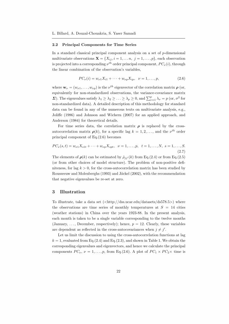
To illustrate, take a data set (<http://dss.ucar.edu/datasets/ds578.5>) where
the observations are time series of monthly temperatures at S = 14 cities
(weather stations) in China over the years 1923-88. In the present analysis,
each month is taken to be a single variable corresponding to the twelve months
(January, . . . , December, respectively); hence, p = 12. Clearly, these variables
are dependent as reflected in the cross-autocovariances when j = j′.
Let us limit the discussion to using the cross-autocorrelation functions at lag
k = 1, evaluated from Eq.(2.4) and Eq.(2.3), and shown in Table 1. We obtain the
corresponding eigenvalues and eigenvectors, and hence we calculate the principal
components PCν , ν = 1, . . . , p, from Eq.(2.6). A plot of PC1 × PC2× time is
22

An Exploratory Analysis of Multiple Multivariate Time Series
displayed in Figure 1, and that for PC1 × PC3× time is given in Figure 2. An
interesting feature of these data highlighted by the methodology is that it is
the PC1 × PC3 pair that distinguishes more readily the city groupings. Figure
3 displays the PC1 × PC3 values for all series and all times without tracking
time (i.e., the 3-dimensional PC1 × PC3 × time values are projected onto the
PC1 × PC3 plane). Hence, we are able to discriminate between cities.
Thus, we observe that cities 1-4 (Hailaer, HaErBin, MuDanJiang and ChangChun,
respectively), color coded in black (and indicated by the symbol black and full
lines (‘lty=1’)) have similar temperatures and are located in the north-eastern
region of China. Cities 5-7 (TaiYuan, BeiJing, TianJin), identified by red ( and
lines − · − (‘lty=4’)), are in the north, and have similar but different tempera-
ture trends than do those in the north-eastern region. Two (BeiJing and TianJin)
are located close to sea-level, while the third (TaiYuan) is further south (and so
might be expected to have higher temperatures) but its elevation is very high so
decreasing its temperature patterns to be more in line with BeiJing and TianJin.
Cities 8-11 (ChengDu, WuHan, ChangSha, HangZhou), green (∗) with lines · · ·(‘lty=3’), are located in central regions with ChengDu further west but elevated.
Finally, cities 12-14 (FuZhou, XiaMen, GuangZhou), blue () with lines −−−(‘lty=8’), are in the southeast part of the country.
Pearson correlations between the variables Xj , j = 1, . . . , 12, and the prin-
cipal components PCν , ν = 1, . . . , 12, sand correlation circles (not shown) show
that all months have an impact on PC1 with the months of June, July and Au-
gust having a slightly negative influence on PC2. Plots for other k = 1 values
give comparable results. Likewise, analyses using the cross-autocorrelations of
Eq.(2.5) also produce similar conclusions.
4 Conclusion
The methodology has successfully identified cities with similar temperature trends,
which trends a priori could not have been foreshadowed, but which do conform
with other geophysical information thus confirming the usefulness of the method-
ology. The cross-autocorrelation functions for a p-dimensional multivariate time
series have been extended to the case where there are S ≥ 1 multivariate time
series. These replaced the standard variance-covariance matrices for use in a
principal component analysis, thus retaining measures of the time dependencies
inherent to time series data. The methodology produces principal component
time series, which can be compared in the usual way on a principal component
plot, except that the plot also includes time as an additional plot dimension.
23

L. Billard, A. Douzal-Chouakria, S. Yaser Samadi
References
Anderson, T.W. (1984): An Introduction to Multivariate Statistical Analysis (2nd
ed), John Wiley, New York.
Billard, L., Douzal-Chouakria, D. and Samadi, S. Y. (2015). Toward Autocorrela-
tion Functions: A Non-Parametric Approach to Exploratory Analysis of Multiple
Multivariate Time Series. Manuscript.
Box, G. E. P., Jenkins, G. M. and Reinsel, G. C. (2011): Time Series Analysis:
Forecasting and Control (4th. ed.). John Wiley, New York.
Brockwell, P.J. and Davis, R.A. (1991): Time Series: Theory and Methods. Springer-
Verlag, New York.
Caiado, J., Maharaj, E. A., D’Urso, P. Time series clustering, in Handbook of Clus-
ter Analysis, Chapman & Hall, C. Hennig, M. Meila, F. Murtagh, R. Rocci (eds.),
in press.
Cryer, J.D. and Chan, K.-S. (2008): Time Series Analysis. Springer-Verlag, New
York.
D’Urso, P., Maharaj, E. A. (2009) Autocorrelation-based Fuzzy Clustering of Time
Series, Fuzzy Sets and Systems, 160, 35653589. DOI: 10.1016/j.fss.2009.04.013.
Jackel, P. (2002): Monte Carlo Methods in Finance. John Wiley, New York.
Johnson, R.A. and Wichern, D.W. (2007): Applied Multivariate Statistical Analysis
(7th ed.), Prentice Hall, New Jersey.
Joliffe, I.T. (1986): Principal Component Analysis, Springer-Verlag, New York.
Jones, R.H. (1964): Prediction of multivariate time series. Journal of Applied Me-
teorology, 3, 285-289.
Kosmelj, K. and Batagelj, V. (1990): Cross-sectional approach for clustering time
varying data. Journal of Classification 7, 99-109.
Liao, T.W. (2005): Clustering of time series - a survey. Pattern Recognition 38,
1857-1874.
Liao, T.W. (2007): A clustering procedure for exploratory mining of vector time
series. Pattern Recognition 40, 2550-2562.
Rousseeuw, P. and Molenberghs, G. (1993): Transformation of non positive
semidefnite correlation matrices. Communications in Statistics - Theory and Meth-
ods 22, 965-984.
Whittle, P. (1963): On the fitting of multivariate autoregressions, and the approxi-
mate canonical factorization of a spectral density matrix. Biometrika 50, 129-134.
24

An Exploratory Analysis of Multiple Multivariate Time Series
Table 1 - Sample Cross-Autocorrelations - ρ(k), k = 1
Sample Cross-Autocorrelations ρjj′(1)
Xj X1 X2 X3 X4 X5 X6 X7 X8 X9 X10 X11 X12
X1 0.965 0.963 0.947 0.938 0.924 0.883 0.851 0.888 0.942 0.959 0.961 0.964
X2 0.960 0.959 0.954 0.942 0.926 0.882 0.850 0.887 0.935 0.950 0.958 0.957
X3 0.952 0.952 0.948 0.937 0.925 0.876 0.840 0.882 0.929 0.940 0.947 0.948
X4 0.943 0.945 0.941 0.936 0.929 0.883 0.846 0.877 0.923 0.932 0.935 0.940
X5 0.921 0.923 0.922 0.924 0.926 0.894 0.841 0.870 0.916 0.918 0.915 0.915
X6 0.886 0.888 0.890 0.891 0.897 0.882 0.852 0.871 0.895 0.889 0.877 0.878
X7 0.849 0.845 0.849 0.847 0.850 0.855 0.894 0.912 0.887 0.865 0.857 0.848
X8 0.890 0.883 0.877 0.879 0.877 0.870 0.906 0.927 0.922 0.904 0.899 0.891
X9 0.943 0.938 0.922 0.921 0.915 0.895 0.892 0.923 0.960 0.958 0.950 0.946
X10 0.960 0.953 0.938 0.931 0.921 0.891 0.869 0.906 0.956 0.964 0.963 0.958
X11 0.970 0.960 0.947 0.936 0.921 0.879 0.862 0.897 0.952 0.961 0.962 0.963
X12 0.969 0.960 0.948 0.933 0.920 0.878 0.849 0.889 0.946 0.959 0.962 0.961
−400 −200 0 200 400 600 800−54
0−
520
−50
0−
480
−46
0−
440
−42
0−
400
010
2030
4050
6070
PC1
PC2
Time
Cities 1−4
Cities 5−7 Cities 8−11
Cities 12−14
Figure 1 - Temperature Data: PC1 × PC2 over Time – All Cities, k = 1
25

L. Billard, A. Douzal-Chouakria, S. Yaser Samadi
−400 −200 0 200 400 600 800−20
0−
150
−10
0 −
50
0
0
10
20
30
40
50
60
70
PC1
PC3
Time
Cities 1−4
Cities 5−7
Cities 8−11
Cities 12−14
Figure 2 - Temperature Data: PC1 × PC3 over Time – All Cities, k = 1
−400 −200 0 200 400 600
−150
−100
−50 Cities 1−4
Cities 5−7
Cities 8−11
Cities 12−14
PC1
PC3
Figure 3 - Temperature Data: PC1 × PC3 – All Cities, All Times, k = 1
26
Proceedings 1st International Workshop on Advanced Analytics and Learning on Temporal DataAALTD 2015
Symbolic Representation of Time Series: a
Hierarchical Coclustering Formalization
Alexis Bondu1, Marc Boullé2, Antoine Cornuéjols31 EDF R&D, 1 avenue du Général de Gaulle 92140 Clamart, France
2 Orange Labs, 2 avenue Pierre Marzin 22300 Lannion, France3 AgroParisTech, 16 rue Claude Bernard 75005 Paris, France
Abstract. The choice of an appropriate representation remains crucialfor mining time series, particularly to reach a good trade-o between thedimensionality reduction and the stored information. Symbolic represen-tations constitute a simple way of reducing the dimensionality by turningtime series into sequences of symbols. SAXO is a data-driven symbolicrepresentation of time series which encodes typical distributions of datapoints. This approach was rst introduced as a heuristic algorithm basedon a regularized coclustering approach. The main contribution of this ar-ticle is to formalize SAXO as a hierarchical coclustering approach. Thesearch for the best symbolic representation given the data is turned intoa model selection problem. Comparative experiments demonstrate thebenet of the new formalization, which results in representations thatdrastically improve the compression of data.
Keywords: Time series, symbolic representation, coclustering
1 Introduction
The choice of the representation of time series remains crucial since it impactsthe quality of supervised and unsupervised analysis [1]. Time series are partic-ularly dicult to deal with due to their inherently high dimensionality whenthey are represented in the time-domain [2] [3]. Virtually all data mining andmachine learning algorithms scale poorly with the dimensionality. During thelast two decades, numerous high level representations of time series have beenproposed to overcome this diculty. The most commonly used approaches are:the Discrete Fourier Transform [4], the Discrete Wavelet Transform [5] [6], theDiscrete Cosine Transform [7], the Piecewise Aggregate Approximation (PAA)[8]. Each representation of time series encodes some information derived fromthe raw data4. According to [1], mining time series heavily relies on the choice ofa representation and a similarity measure. Our objective is to nd a compact
and informative representation which is driven by the data. The symbolic rep-resentations constitute a simple way of reducing the dimensionality of the databy turning time series into sequences of symbols [9]. In such representations, eachsymbol corresponds to a time interval and encodes information which summarize
4 Raw data designates a time series represented in the time-domain by a vector ofreal values.
Copyright c⃝2015 for this paper by its authors. Copying permitted for private and academicpurposes.
27

A. Bondu, M. Boullé, A. Cornuéjols
the related sub-series. Without making hypothesis on the data, such a represen-tation does not allow one to quantify the loss of information. This article focuseson a less prevalent symbolic representation which is called SAXO5. This approachoptimally discretizes the time dimension and encodes typical distributions6 ofdata points with the symbols [10]. SAXO oers interesting properties. Since thisrepresentation is based on a regularized Bayesian coclustering7 approach calledMODL8 [11], a good trade-o is naturally reached between the dimensionalityreduction and the information loss. SAXO is a parameter-free and data-drivenrepresentation of time series. In practice, this symbolic representation proves tobe highly informative for training classiers. In [10], SAXO was evaluated onpublic datasets and favorably compared with the SAX representation.
Originally, SAXO was dened as a heuristic algorithm. The two main con-tributions of this article are: i) the formalization of SAXO as a hierarchicalcoclustering approach; ii) the evaluation of its compactness in terms of cod-ing length. This article is organized as follows. Section 2 briey introduces thesymbolic representations of time series and presents the original SAXO heuristicalgorithm. Section 3 formalizes the SAXO approach resulting in a new evalu-ation criterion which is the main contribution of this article. Experiments areconducted in Section 4 on real datasets in order to compare the SAXO evalua-tion criterion with that of the MODL coclustering approach. Lastly, perspectivesand future works are discussed in Section 5.
2 Related work
Numerous compact representations of time series deal with the curse of dimen-sionality by discretizing the time and by summarizing the sub-series within eachtime interval. For instance, the Piecewise Aggregate Approximation (PAA) en-codes the mean values of data points within each time interval. The PiecewiseLinear Approximation (PLA) [12] is an other example of compact representa-tion which encodes the gradient and the y-intercept of a linear approximation ofsub-series. In both cases, the representation consist of numerical values which de-scribe each time interval. In contrast, the symbolic representations characterizethe time intervals by categorical variables [9]. For instance, the Shape Deni-tion Language (SDL) [13] encodes the shape of sub-series by symbols. The mostcommonly used symbolic representation is the SAX9 approach [9]. In this case,the time dimension is discretized into regular intervals, the symbols encode themean values per interval.
5 SAXO Symbolic Aggregate approXimation Optimized by data.6 The SAXO approach produces clusters of time series within each time interval whichcorrespond to the symbols.
7 The coclustering problem consist in reordering rows and columns of a matrix in orderto satisfy a homogeneity criterion.
8 Minimum Optimized Description Length9 Symbolic Aggregate approXimation.
28

Symbolic Representation of TS: a Hierarchical Coclustering Approach
The symbolic representations appear to be really helpful for processing largedatasets of time series owing to dimensionality reduction. However, these ap-proaches suer several limitations.
Most of these representations are lossy compression approaches unable toquantify the loss of information without strong hypothesis on the data.
The discretization of the time dimension into regular intervals is not datadriven.
The symbols have the same meaning over time irrespectively of their rank(i.e. the ranks of the symbols may be used to improve the compression).
Most of these representations involve user parameters which aect the storedinformation (ex: for the SAX representation, the number of time intervalsand the size of the alphabet must be specied).
The SAXO approach overcomes these limitations by optimizing the timediscretization, and by encoding typical distributions of data points within eachtime interval [10]. SAXO was rst dened as a heuristic which exploits the MODLcoclustering approach.
Fig. 1. Main steps of the SAXO learning algorithm.
Figure 1 provides an overview of this approach by illustrating the main stepsof the learning algorithm. The joint distribution of the identiers of the timeseries C, the values X, and the timestamp T is estimated by a trivariate coclus-tering model. The time discretization resulting from the rst step is retained,and the joint distribution of X and C is estimated within each time interval byusing a bivariate coclustering model. The resulting clusters of time series arecharacterized by piecewise constant distributions of values and correspond tothe symbols. A specic representation allows one to re-encode the time series asa sequence of symbols. Then, the typical distribution that best represents thedata points of the time series is selected within each time interval. Figure 2(a)plots an example of recoded time series. The original time series (represented bythe blue curve) is recoded by the abba SAXO word. The time is discretizedinto four intervals (the vertical red lines) corresponding to each symbol. Withintime intervals, the values are discretized (the horizontal green lines): the numberof intervals of values and their locations are not necessary the same. The sym-bols correspond to typical distributions of values: conditional probabilities of Xare associated with each cell of the grid (represented by the gray levels); Figure2(b) gives an example of the alphabet associated with the second time interval.The four available symbols correspond to typical distributions which are both
29

A. Bondu, M. Boullé, A. Cornuéjols
represented by gray levels and by histograms. By considering Figures 2(a) and2(b), b appears to be the closest typical distribution of the second sub-series.
(a) (b)
Fig. 2. Example of a SAXO representation (a) and the alphabet of the second timeinterval (b).
As in any heuristic approach, the original algorithm nds a suboptimal solu-tion for selecting the most suitable SAXO representation given the data. Solvingthis problem in an exact way appears to be intractable, since it is comparableto the coclustering problem which is NP-hard. The main contribution of thispaper is to formalize the SAXO approach within the MODL framework. Weclaim this formalization is a rst step to improving the quality of the SAXOrepresentations learned from data. In this article, we dene a new evaluationcriterion denoted by Csaxo (see Section 3). The most probable SAXO represen-tation given the data is dened by minimizing Csaxo. We expect to reach betterrepresentations by optimizing Csaxo, instead of exploiting the original heuristicalgorithm.
3 Formalization of the SAXO approach
This section presents the main contribution of this article: the SAXO ap-proach is formalized as a hierarchical coclustering approach. As illustrated inFigure 3, the originality of the SAXO approach is that the groups of identiers(variable C) and the intervals of values (variable X) are allowed to change overtime. By contrast, the MODL coclustering approach forces the discretization ofC and X to be the same within time intervals. Our objective is to reach bettermodels by removing this constraint.
A SAXO model is hierarchically instantiated by following two successivesteps. First, the discretization of time is determined. The bivariate discretiza-tion C × X is then dened within each time interval. Additional notations arerequired to describe the sequence of bivariate data grids.
30

Symbolic Representation of TS: a Hierarchical Coclustering Approach
X
C
T
MODL coclusteringX
C
T
SAXO
Fig. 3. Examples of a MODL coclustering model (left part) and a SAXO model (rightpart).
Notations for time series: In this article, the input dataset D is consid-ered to be a collection of N time series denoted Si (with i ∈ [1, N ]). Eachtime series consists of mi data points, which are couples of values X andtimestamps T . The total number of data points is denoted by m =
∑Ni=1 mi.
Notations for the t-th time interval of a SAXO model:
kT : number of time intervals; ktC : number of clusters of time series; ktX : number of intervals of value; kC(i, t): index of the cluster that contains the sub-series of Si; nt
iC: number of time series in each cluster itC ;
mt: number of data point; mt
i: number of data points of each time series Si; mt
iC: number of data points in each cluster itC ;
mtjX
: number of data points in the intervals jX ; mt
iCjX: number of data points belonging to each cell (iC , jX).
Eventually, a SAXO model M ′ is rst dened by a number of time intervalsand the location of their bounds. The bivariate data grids C × X within eachtime interval are dened by: i) the partition of the time series into clusters; ii)the number of intervals of values; iii) the distribution of the data points on thecells of the data grid; iv) for each cluster, the distribution of the data pointson the time series belonging to the same cluster. Section 3.1 presents the priordistribution of the SAXO models. The likelihood of a SAXO model given thedata is described in Section 3.2. A new evaluation criterion which denes themost probable model given the data is proposed in Section 3.3.
3.1 Prior distribution of the SAXO models
The proposed prior distribution P (M ′) exploits the hierarchy of the parametersof the SAXO models and is uniform at each level. The prior distribution of thenumber of time intervals kT is given by Equation 1. The parameter kT belongs to[1,m], with m representing the total number of data points. All possible values
31

A. Bondu, M. Boullé, A. Cornuéjols
of kT are considered as equiprobable. By using combinatorics, the number ofpossible locations of the bounds can be enumerated given a xed value of kT .Once again, all possible locations are considered as equiprobable. Equation 2represents the prior distribution of the parameter mt given kT . Within eachtime interval t, the number of intervals of values ktX is uniformly distributed(see Equation 3). The value of ktX belongs to [1,mt], with mt representing thenumber of data points within the t-th time interval. All possible values of ktX areequiprobable. The same approach is applied to dene the prior distribution of thenumber of clusters within each time interval (see Equation 4). The value of ktCbelongs to [1, N ], with N denoting the total number of time series. Once again,all possible values of ktC are equiprobable. The possible ways of partitioningthe N time series into ktC clusters can be enumerated, given a xed number ofclusters in the t-th time interval. The term B(N, ktC) in Equation 5 represents thenumber of possible partitions of N elements into ktC possibly empty clusters10.Within each time interval, all distributions of the mt data points on the cellsof the bivariate data grid C × X are considered as equiprobable. Equation 6enumerates the possible ways of distributing mt data points on ktX .ktC cells.Given a time interval t and a cluster itC , all distributions of the data pointson the time series belonging to the same cluster are equiprobable. Equation 7enumerates the possible ways of distributing mt
i data points on ntiC
time series.
P (kT ) =1
m(1) P (mt|kT ) =
1(m+kT−1
kT−1
)(2)
P (ktX|kT , mt) =
kT∏t=1
1
mt(3)
P (ktC|kT ) =
kT∏t=1
1
N(4) P
(kC(i, t)|kT , kt
C)=
kT∏t=1
1
B(N, ktC)
(5)
P(mt
jC ,jX|kT , mt, ktX, kt
C)=
kT∏t=1
1(mt+ktC.kt
X−1
ktC.kt
X−1
) (6)
P(mt
i|kT , ktC, kC(i, t), mt
jC ,jX)=
kT∏t=1
ktC∏
i=1
1(mtiC
+ntiC
−1
ntiC
−1
) (7)
In the end, the prior distribution of the SAXO models M ′ is given by Equa-tion 8.
P (M ′) =1
m× 1(
m+kT−1kT−1
) ×kT∏t=1
[1
mt× 1
N× 1
B(N, ktC)
× 1(mt+ktC.kt
X−1
ktC.kt
X−1
) ×ktC∏
i=1
1(mtiC
+ntiC
−1
ntiC
−1
)
(8)
10 The second kind of Stirling numbers Svk
enumerates the possible partitions of v
elements into k clusters and B(N, ktC) =
∑ktC
i=1 SNi
.
32
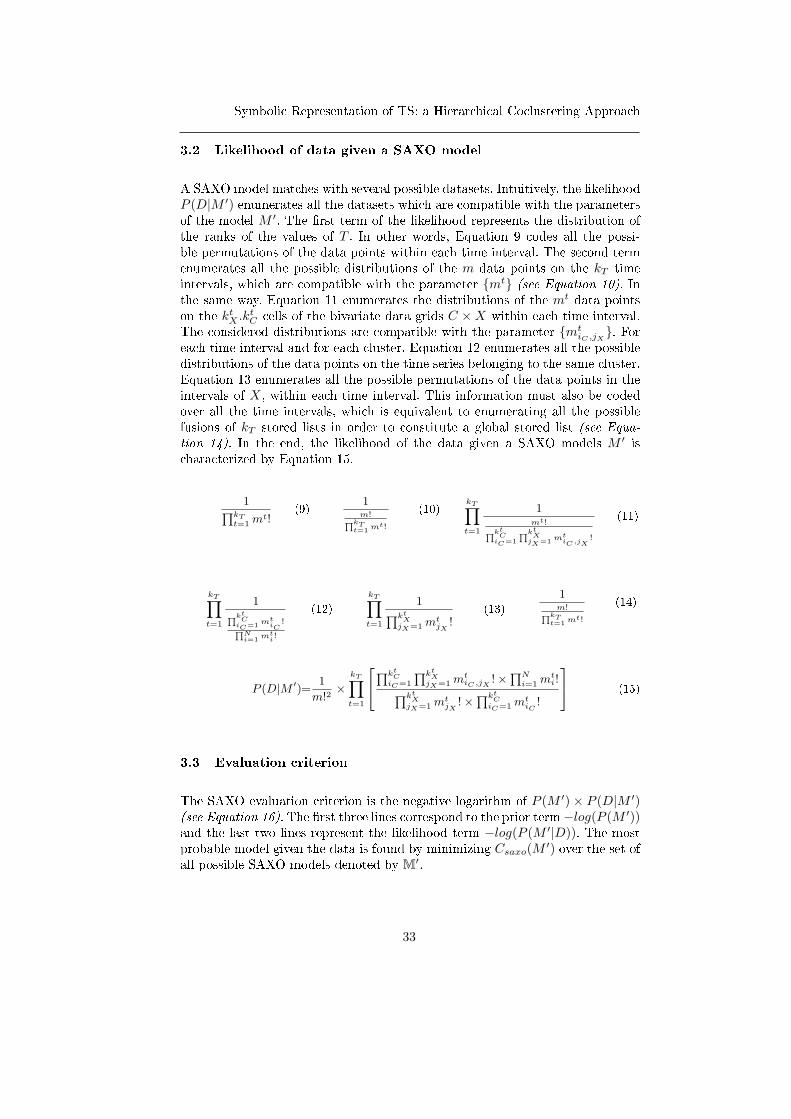
Symbolic Representation of TS: a Hierarchical Coclustering Approach
3.2 Likelihood of data given a SAXO model
A SAXO model matches with several possible datasets. Intuitively, the likelihoodP (D|M ′) enumerates all the datasets which are compatible with the parametersof the model M ′. The rst term of the likelihood represents the distribution ofthe ranks of the values of T . In other words, Equation 9 codes all the possi-ble permutations of the data points within each time interval. The second termenumerates all the possible distributions of the m data points on the kT timeintervals, which are compatible with the parameter mt (see Equation 10). Inthe same way, Equation 11 enumerates the distributions of the mt data pointson the ktX .ktC cells of the bivariate data grids C ×X within each time interval.The considered distributions are compatible with the parameter mt
iC ,jX. For
each time interval and for each cluster, Equation 12 enumerates all the possibledistributions of the data points on the time series belonging to the same cluster.Equation 13 enumerates all the possible permutations of the data points in theintervals of X, within each time interval. This information must also be codedover all the time intervals, which is equivalent to enumerating all the possiblefusions of kT stored lists in order to constitute a global stored list (see Equa-tion 14). In the end, the likelihood of the data given a SAXO models M ′ ischaracterized by Equation 15.
1∏kTt=1 m
t!(9)
1m!∏kT
t=1 mt!
(10)kT∏t=1
1mt!∏kt
CiC=1
∏ktX
jX=1 mtiC,jX
!
(11)
kT∏t=1
1∏ktC
iC=1 mtiC
!∏Ni=1 mt
i !
(12)
kT∏t=1
1∏ktX
jX=1 mtjX
!(13)
1m!∏kT
t=1 mt!
(14)
P (D|M ′)=1
m!2×
kT∏t=1
∏ktC
iC=1
∏ktX
jX=1 mtiC ,jX
!×∏N
i=1 mti!∏kt
XjX=1 m
tjX
!×∏kt
CiC=1 m
tiC!
(15)
3.3 Evaluation criterion
The SAXO evaluation criterion is the negative logarithm of P (M ′)× P (D|M ′)(see Equation 16). The rst three lines correspond to the prior term−log(P (M ′))and the last two lines represent the likelihood term −log(P (M ′|D)). The mostprobable model given the data is found by minimizing Csaxo(M
′) over the set ofall possible SAXO models denoted by M′.
33

A. Bondu, M. Boullé, A. Cornuéjols
Csaxo(M′) = log(m) + log
(m+ kT − 1
kT − 1
)+
kT∑t=1
log(mt)
+kT .log(N)+
kT∑t=1
log(B(N, kt
C))+
kT∑t=1
log
(mt+kt
C .ktX−1
ktC .k
tX − 1
)
+
kT∑t=1
ktC∑
iC=1
log
(mt
iC+ nt
iC− 1
ntiC
− 1
)
+ 2.log(m!)−kT∑t=1
ktC∑
iC=1
ktX∑
jX=1
log(mtiC ,jX !)
+
kT∑t=1
ktC∑
iC=1
log(mtiC !)−
N∑i=1
log(mti!) +
ktX∑
jX=1
log(mtjX !)
(16)
Key ideas to retain: Rather than having a heuristic decomposition of theSAXO approach in a two-step algorithm, we propose a single evaluation cri-terion based on the MODL framework. Once optimized, this criterion shouldyield better representations of time series. We compare the ability of bothcriterion to compress data. We aim at evaluating the interest of optimizingCsaxo rather than the original trivariate coclustering criterion [14] (denotedby Cmodl).
4 Comparative experiments on real datasets
According to the information theory and since both criteria are a negative loga-rithm of a probability, Csaxo and Cmodl represent the coding length of the models.In this section, both approaches are compared in terms of coding length. The20 processed datasets come from the UCR Time Series Classication and Clus-tering repository [15]. Some datasets are relatively small, we have selected theones which include at least 800 learning examples. Originally, these datasets aredivided into training and test sets which have been merged in our experiments.The objective of this section is to compare Csaxo and Cmodl for each dataset.On the one hand, the criterion Cmodl is optimized by using the greedy heuristicand a neighborhood exploration mentioned described in [11]. The coding lengthof the most probable MODL model (denoted by MAPmodl) is then calculated byusing Cmodl. On the other hand, the criterion Csaxo is optimized by exploitingthe original heuristic algorithm illustrated in Figure 1 [10]. The coding lengthof best SAXO model (denoted by MAPsaxo) is given by the criterion Csaxo. No-tice that both algorithms have a O(m
√m logm) time complexity. The order of
magnitude of the coding length depends on the size of the data set and can notbe easily compared over all datasets. We choose to exploit the compression gain[16] which consists in comparing the coding length of a model M with the coding
34

Symbolic Representation of TS: a Hierarchical Coclustering Approach
length of the simplest model Msim. This key performance indicator varies in theinterval [0, 1]. The compression gain is similarly dened for the MODL and theSAXO approaches such that:
Gainmodl(M) = 1− Cmodl(M)/Cmodl(Msim)
Gainsaxo(M′) = 1− Csaxo(M
′)/Csaxo(Msim)
Our experiments evaluate the variation of the compression gain between theSAXO and the MODL approaches. This indicator is denoted by ∆G and rep-resents the relative improvement of the compression gain provided by SAXO.The value of ∆G can be negative, which means that SAXO provides a worsecompression gain than the MODL approach.
∆G =Gainsaxo(MAPsaxo)− Gainmodl(MAPmodl)
Gainmodl(MAPmodl)
Dataset ∆G Dataset ∆G
Starlight curves 63.86% CBF −1.43%uWaveGestureX 191.41% AllFace 383.24%uWaveGestureY 157.79% Symbols 23.16%uWaveGestureZ 185.13% 50 Words 400.68%ECG Five Days −1.80% Wafer 37.03%MoteStrain 627.84% Yoga 63.40%
CincEGCtorso 32.93% FacesUCR −18.39%MedicalImages 191.32% Cricket Z 290.22%WordSynonym 264.93% Cricket X 285.87%TwoPatterns missing Cricket Y 296.40%
Table 1. Coding length evaluation.
Table 1 presents the results of our experiments and includes a particularcase with a missing value for the dataset TwoPatterns. In this case, the rststep of the heuristic algorithm which optimizes Csaxo (see Figure 1) leads to thesimplest trivariate coclustering model that includes a single cell. This is a sideeect due to the fact that the MODL approach is regularized. A possible expla-nation is that the temporal representation of time series is not informative forthis dataset. Other representations such as the Fourier or the wavelet transformscould be tried. In most cases, ∆G has a positive value which means SAXO pro-vides a better compression than the MODL approach. This trend emerges clearly,the average compression improvement reaches 183%. We exploit the Wilcoxonsigned-ranks test to reliably comparing both approaches over all datasets [17]. Ifthe output value (denoted by z) is smaller than −1.96, the gap in performanceis considered as signicant. Our experiments give z = −3.37 which is highlysignicant. In the end, the compression of data provided by SAXO appears tobe intrinsically better than the MODL approach. The prior term of Csaxo in-duces an additional cost in terms of coding length. This additional cost is faroutweighed by a better encoding of the likelihood.
35

A. Bondu, M. Boullé, A. Cornuéjols
5 Conclusion and perspectives
SAXO is a data-driven symbolic representation of time series which extendsSAX in three ways: i) the discretization of time is optimized by a Bayesianapproach rather than considering regular intervals; ii) the symbols within eachtime interval represents typical distributions of data points rather than averagevalues; iii) the number of symbols may dier per time interval. The parametersettings is automatically optimized given the data. SAXO was rst introduced asan heuristic algorithm. This article formalizes this approach within the MODLframework as a hierarchical coclustering approach (see Section 3). A Bayesianapproach is applied leading to an analytical evaluation criterion. This criterionmust be minimized in order to dene the most probable representation given thedata. This new criterion is evaluated on real datasets in Section 4. Our experi-ments compare the SAXO representation with the original MODL coclusteringapproach. The SAXO representation appears to be signicantly better in termsof data compression. In future work, we plan to use the SAXO criterion in orderto dene a similarity measure. Numerous learning algorithms, such as K-meansand K-NN, could use such an improved similarity measure dened over timeseries. We plan to explore potential gains in areas such as: i) the detection ofatypical time series; ii) the query of a database by similarity; iii) the clusteringof time series.
References
1. T. Liao, Clustering of time series data: a survey, Pattern Recognition, vol. 38, pp.18571874, 2005.
2. D. Bosq, Linear Processes in Function Spaces: Theory and Applications (LectureNotes in Statistics). Springer, 2000.
3. J. Ramsay and B. Silverman, Functional Data Analysis, ser. Springer Series inStatistics. Springer, 2005.
4. M. Frigo and S. Johnson, The design and implementation of FFTW3, Proceedingsof the IEEE, vol. 93, no. 2, pp. 216231, 2005, special issue on Program Generation,Optimization, and Platform Adaptation.
5. R. Polikar, Physics and Modern Topics in Mechanical and Electrical Engineering.World Scientic and Eng. Society Press, 1999, ch. The story of wavelets.
6. K. Chan and W. Fu, Ecient Time Series Matching by Wavelets, in ICDE '99:Proceedings of the 15th International Conference on Data Engineering. IEEEComputer Society, 1999.
7. N. Ahmed, T. Natarajan, and K. R. Rao, Discrete Cosine Transfom, IEEE Trans.Comput., vol. 23, no. 1, pp. 9093, 1974.
8. C. Guo, H. Li, and D. Pan, An improved piecewise aggregate approximation basedon statistical features for time series mining, in Proceedings of the 4th internationalconference on Knowledge science, engineering and management, ser. KSEM'10.Berlin, Heidelberg: Springer-Verlag, 2010, pp. 234244.
9. J. Lin, E. Keogh, S. Lonardi, and B. Chiu, A Symbolic Representation of TimeSeries, with Implications for Streaming Algorithms, in 8th ACM SIGMOD Work-shop on Research Issues in Data Mining and Knowledge Discovery, San Diego,2003.
36

Symbolic Representation of TS: a Hierarchical Coclustering Approach
10. A. Bondu, M. Boullé, and B. Grossin, SAXO : An Optimized Data-driven Sym-bolic Representation of Time Series, in IJCNN (International Joint Conferenceon Neural Networks). IEEE, 2013.
11. M. Boullé, Hands on pattern recognition. Microtome, 2010, ch. Data grid modelsfor preparation and modeling in supervised learning.
12. H. Shatkay and S. B. Zdonik, Approximate Queries and Representations for LargeData Sequences, in 12th International Conference on Data Engineering (ICDE),1996, pp. 536545.
13. R. Agrawal, G. Psaila, E. L. Wimmers, and M. Zait, Querying Shapes of His-tories, in 21th International Conference on Very Large Data Bases (VLDB 95),1995, pp. 502514.
14. M. Boullé, Functional data clustering via piecewise constant nonparametric den-sity estimation, Pattern Recognition, vol. 45, no. 12, pp. 43894401, 2012.
15. E. Keogh, Q. Zhu, B. Hu, H. Y., X. Xi, L. Wei, and C. A. Ratanama-hatana, The UCR Time Series Classication/Clustering Homepage :www.cs.ucr.edu/∼eamonn/time_series_data/, 2011.
16. M. Boullé, Optimum simultaneous discretization with data grid models in su-pervised classication: a Bayesian model selection approach, Advances in DataAnalysis and Classication, vol. 3, no. 1, pp. 3961, 2009.
17. J. Dem²ar, Statistical Comparisons of Classiers over Multiple Data Sets, Journalof Machine Learning Research, vol. 7, pp. 130, Dec. 2006.
37

38
Proceedings 1st International Workshop on Advanced Analytics and Learning on Temporal DataAALTD 2015
Temporal and Frequential Metric Learning
for Time Series kNN Classification
Cao-Tri Do123, Ahlame Douzal-Chouakria2, Sylvain Marié1, and MichèleRombaut3
1 Schneider Electric, France2 LIG, University of Grenoble Alpes, France
3 GIPSA-Lab, University of Grenoble Alpes, France
Abstract. This work proposes a temporal and frequential metric learn-ing framework for a time series nearest neighbor classification. For that,time series are embedded into a pairwise space where a combinationfunction is learned based on a maximum margin optimization process.A wide range of experiments are conducted to evaluate the ability of thelearned metric on time series kNN classification.
Keywords: Metric learning, Time series, kNN, Classification, Spectral metrics.
1 Introduction
Due to their temporal and frequential nature, time series constitute complexdata to analyze by standard machine learning approaches [1]. In order to clas-sify such challenging data, distance features must be used to bring closer timeseries of identical classes and separate those of different classes. Temporal datamay be compared on their values. The most frequently used value-based met-rics are the Euclidean distance and the Dynamic Time Warping dtw to copewith delays [2,3]. They can also be compared on their dynamics and frequentialcharacteristics [4, 5]. Promising approaches aims to learn the Mahalanobis dis-tance or kernel function for a specific classifier [6,7]. Other work investigate therepresentation paradigm by representating objects in a dissimilarity space whereare investigated dissimilarity combinations and metric learning [8, 9]. The ideain this paper is to combine basic metrics into a discriminative one for a kNNclassifier. In the metric learning context for a metric learning approach drivenby nearest neighbors (Weinberger & Saul [6]), we extend the work of Do & al.in [10] to temporal and frequential characteristics. The main idea is to embedpairs of time series in a space whose dimensions are basic temporal and frequen-tial metrics, where a combination function is learned based on a large marginoptimization process.
The main contributions of the paper are a) propose a new temporal and fre-quential metric learning framework for a time series nearest neighbors classifica-tion, b) learn a combination metric involving amplitude, behavior and frequen-tial characteristics and c) conduct large experimentations to study the ability oflearned metric. The rest of the paper is organized as follows. Section 2 recallsbriefly the major metrics for time series. In Section 3, we present the proposed
Copyright c©2015 for this paper by its authors. Copying permitted for private and academicpurposes.
39

C.-T. Do, A. Douzal-Chouakria, S. Marié, M. Rombaut
metric learning approach. Finally, Section 4 presents the experiments conductedand discusses the results obtained.
2 Time series metrics
Let xi = (xi1, ..., xiT ) and xj = (xj1, ..., xjT ) be two time series of time lengthT . Time series metrics fall at least within three main categories. The first oneconcerns value-based metrics, where time series are compared according to theirvalues regardless of their behaviors. Among these metrics are the Euclideandistance (dE), the Minkowski distance and the Mahalanobis distance [3]. Werecall the formula of dE :
dE(xi,xj) =
√√√√
T∑
t=1
(xit − xjt)2 (1)
The second category relies on metrics in the spectral representations. In someapplications, time series may be similar because they share the same frequencycharacteristics. For that, time series xi are first transformed into their Fourierrepresentation xi = [xi1, ..., xiF ], where xif is a complex number (i.e. Fourier
components), with F = 2T
2+ 1 [5]. Then, one may use the Euclidean distance
(dFFT ) between the module of the complex numbers xif , noted |xif |:
dFFT (xi,xj) =
√√√√
F∑
f=1
(|xif | − |xjf |)2 (2)
Note that times series of similar frequential characteristics may have distinctiveglobal behavior. Thus, to compare time series based on their behavior, a thirdcategory of metrics is used. Many applications refer to the Pearson correlationor its generalization, the temporal correlation coefficient [4] defined as:
Cortr(xi,xj) =
∑
t,t′(xit − xit′)(xjt − xjt′)
√∑
t,t′(xit − xit′)2
√∑
t,t′(xjt − xjt′)2
(3)
where |t−t′| ≤ r, r ∈ [1, ..., T −1] being a parameter that can be learned or fixeda priori. The optimal value of r is noisy dependant. For r = T − 1, Eq. 3 leadsto the Pearson correlation. As Cortr is a similarity measure, it is transformedinto a dissimilarity measure: dCortr (xi,xj) =
1
2(1− Cortr(xi,xj)).
3 Temporal and frequential metric learning for a large
margin kNN
Let X = xi, yiNi=1
be a set of N static vector samples, xi ∈ Rp, p being the
number of descriptive features and yi the class labels. Weinberger & Saul pro-posed in [6] an approach to learn a dissimilarity metric D for a large margin
40

Temporal and Frequential Metric Learning for Time Series kNN Classification
kNN. It is based on two intuitions: first, each training sample xi should have thesame label yi as its k nearest neighbors; second, training samples with differentlabels should be widely separated. For this, they introduced the concept of target
for each training sample xi. Target neighbors of xi, noted j i, are the k closestxj of the same class (yj = yi). The target neighborhood is defined with respectto an initial metric. The aim is to learn a metric D that pulls the targets andpushes the ones of different class.
Let d1, ..., dh..., dp be p given dissimilarity metrics that allow to compare sam-ples. The computation of a metric always takes into account a pair of samples.Therefore, we used the pairwise representation introduced in Do & al. [10]. Inthis space, a vector xij represents a pair of samples (xi,xj) described by the p
basics metrics dh: xij = [d1(xi,xj), ..., dp(xi,xj)]T . If xij = 0 then xj is identi-
cal to xi according to all metrics dh. A combination function D of the metricsdh can be seen as a function in this space. We propose in the following to use alinear combination of dh: Dw(xi,xj) =
∑
h wh.dh(xi,xj). Its pairwise notationis Dw(xij) = wT .xij . To ensure that Dw is a valid metric, we set wh ≥ 0 for allh = 1...p. The main steps of the proposed approach to learn the metric, detailedhereafter, can be summarized as follows:
1. Embed each pair (xi,xj) into the pairwise space Rp.
2. Scale the data within the pairwise space.3. Define for each xi its targets.4. Scale the neighborhood of each xi.5. Learn the combined metric Dw.
Data scaling. This operation is performed to scale the data within the pairwisespace and ensure comparable ranges for the p basic metrics dh. In our experiment,we use dissimilarity measures with values in [0; +∞[. Therefore, we propose toZ-normalize their log distributions.
Target set. For each xi, we define its target neighbors as the k nearest neighborsxj (j i) of the same class according to an initial metric. In this paper, we
choose a L2-norm of the pairwise space as the initial metric (√∑
h d2
h). Othermetrics could be chosen. We emphasize that target neighbors are fixed a priori
(at the first step) and do not change during the learning process.
Neighborhood scaling. In real datasets, local neighborhoods can have very dif-ferent scales. To make the target neighborhood spreads comparable, we proposefor each xi to scale its neighborhood vectors xij such that the L2-norm of thefarthest target is 1.
Learning the combined metric Dw. Let xij , yijNi,j=1
be the training set withyij = −1 if yj = yi and +1 otherwise. Learning Dw for a large margin kNNclassifier can be formalized as the following optimization problem:
41

C.-T. Do, A. Douzal-Chouakria, S. Marié, M. Rombaut
minw,ξ
∑
i,j i
Dw(xij)
︸ ︷︷ ︸
pull
+C∑
i,j i,l
1 + yil
2.ξijl
︸ ︷︷ ︸
push
s.t. ∀j i, yl 6= yi,
Dw(xil)−Dw(xij) ≥ 1− ξijl
ξijl ≥ 0
wh > 0 ∀h = 1...p
(4)
Note that the "pull" term∑
j i
Dw(xij) =∑
j i
wT .xij = N.k.wT .xij is a L1-
Mahalanobis norm weighted by the average target sample. Therefore, it behaveslike a L1-norm in the optimization problem. The problem is very similar to aC-SVM classification problem. When C is infinite, we have a "strict" problem:the solver will try to find a direction in the pairwise space for which only targetsare in the close neighborhood of each xi, and a maximum margin 1
||w||2.
Let xtest be a new sample to classify and xtest,i (i = 1, ..., N) the correspondingvectors into the pairwise embedding space. After xtest,i normalization accordingto the Data Scaling step, xtest is classified based on a standard kNN and Dw.
4 Experiments
In this section, we compare kNN classifier performances for several metrics onreference time series datasets [11–14] described in Table 1. To compare with thereference results in [3, 11], the experiments are conducted with the same proto-cols as in Do &. al. [10]: k is set to 1; train and test set are given a priori. Due tothe current format to store the data, small datasets with short time series wereretained and the experiments are conducted on one runtime.
In this experimentation, we consider basic metrics dE , dFFT and dCortr then,we learn a combined metric Dw according to the procedure described in Section 3.First, two basic temporal metrics are considered in D2 (dE and dCortr ) as in Do& al. [10]. Second, we consider a combination between temporal and frequentialmetrics in D3 (dE , dCortr and dFFT ). Cplex library [15] has been used to solvethe optimization problem in Eq. 4. We learn the optimal parameter values ofthese metrics by minimizing a leave-one out cross-validation criterion.
As the training dataset sizes are small, we propose a hierarchical error criterion:
1. Minimize the kNN error rate2. Minimize dintra
dinter
if several parameter values obtain the minimum kNN error.
where dintra and dinter stands respectively to the mean of all intraclass andinterclass distances according to the metric at hand. Table 2 gives the range ofthe grid search considered for the parameters. In the following, we consider onlythe raw series and don’t align them using a dtw algorithm for example. For
42

Temporal and Frequential Metric Learning for Time Series kNN Classification
all reported results (Table 3), the best one is indexed with a star and the onessignificantly similar from the best one (Z-test at 1% risk) are in bold [16].
Dataset Nb. Class Nb. Train Nb. Test TS length
SonyAIBO 2 20 601 70MoteStrain 2 20 1252 84GunPoint 2 50 150 150PowerCons 2 73 292 144ECG5Days 2 23 861 136SonyAIBOII 2 27 953 65Coffee 2 28 28 286BME 3 48 102 128UMD 3 46 92 150ECG200 2 100 100 96Beef 5 30 30 470DiatomSizeReduction 4 16 306 345FaceFour 4 24 88 350Lighting-2 2 60 61 637Lighting-7 7 70 73 319OliveOil 4 30 30 570
Table 1. Dataset description giving the number of classes (Nb. Class), the number oftime series for the training (Nb. Train) and the testing (Nb. Test) sets, and the lengthof each time series (TS length).
Method Parameter Parameter range
dCortr r [1, 2, 3, , ..., T ]D2, D3 C [10−3, 0.5, 1, 5, 10, 20, 30, ..., 150]
Table 2. Parameter ranges
From Table 3, we can see that temporal metrics dE and dCortr alone per-forms better one from the other depending on the dataset. Using a frequentialmetric alone such as dFFT brings significant improvements for some datasets(SonyAIBO, GunPoint, PowerCons, ECG5Days). It can be observed that onebasic metric is sufficient on some databases (MoteStrain, GunPoint, PowerCons,ECG5Days). In other cases, learning a combination of these basic metrics reachthe same performances on most datasets or achieve better results (UMD). Thenew approach allows to extend combination functions to many metrics with-out having to cope with additional parameters in grid search and without totest every basic metrics alone to retained the best one. It also extends thework done in [6] for single distance to multiple distances. Adding metrics suchas dFFT improves the performances on some datasets (SonyAIBO, GunPoint,UMD, FaceFour, Lighting-2, Lighting-7) than considering only temporal metrics
43

C.-T. Do, A. Douzal-Chouakria, S. Marié, M. Rombaut
MetricsDataset Basic Learned combined
dE dCortr dFFT D2 D3
SonyAIBO 0.305 0.308 0.258* 0.308 0.259
MoteStrain 0.121* 0.264 0.278 0.210 0.277GunPoint 0.087 0.113 0.027* 0.113 0.073PowerCons 0.370 0.445 0.315* 0.384 0.410ECG5Days 0.203 0.153 0.006* 0.153 0.156SonyAIBOII 0.141 0.142 0.128* 0.142 0.142
Coffee 0.250 0* 0.357 0* 0*
BME 0.128 0.059* 0.412 0.059* 0.078
UMD 0.185* 0.207 0.315 0.207 0.185*
ECG200 0.120 0.070* 0.166 0.070* 0.070*
Beef 0.467 0.300* 0.500 0.300* 0.367
DiatomSizeReduction 0.065* 0.075 0.069 0.075 0.075
FaceFour 0.216 0.216 0.239 0.216 0.205*
Lighting-2 0.246 0.246 0.148* 0.246 0.213
Lighting-7 0.425 0.411 0.315 0.411 0.288*
OliveOil 0.133* 0.133* 0.200 0.133* 0.133*
Table 3. Error rate of 1NN classifier for different metrics. D2 is computed using dEand dCortr ; D3 uses the 3 basic metrics. The metric with the best performance foreach dataset is indicated by a star (*) and the ones with equivalent performances arein bold.
(dE , dCortr ). However, it does not always improve the results (GunPoint, Pow-erCons, ECG5Days). This might be caused by the fact that our framework issensitive to the choice of the initial metric (L2-norm) or maybe, some steps inthe algorithm should be improved to make the combination better.
5 Conclusion
For nearest neighbor time series classification, we propose to learn a metric as acombination of temporal and frequential metrics based on a large margin opti-mization process. The learned metric shows good performances on the conductedexperimentations. For future work, we are looking for some improvements. First,the choice of the initial metric is crucial. It has been set here as the L2-normof the pairwise space but a different metric could provide better target sets.Otherwise, using an iterative procedure (reusing Dw to generate new target setsand learn Dw again) could be another solution. Second, we note that the L1-norm on the "pull" term leads to sparcity. Changing it into a L2-norm couldallow for non-sparse solutions and also extend the approach to non-linear metriccombination functions thanks to the Kernel trick. Finally, we could extend thisframework to multivariate, regression or clustering problems.
44

Temporal and Frequential Metric Learning for Time Series kNN Classification
References
1. T.C. Fu, “A review on time series data mining,” Engineering Applications of
Artificial Intelligence, 2011.2. H. Sakoe and S. Chiba, “Dynamic Programming Algorithm Optimization for Spo-
ken Word Recognition,” IEEE transactions on acoustics, speech, and signal pro-
cessing, 1978.3. H. Ding, G. Trajcevski, and P. Scheuermann, “Querying and Mining of Time Series
Data : Experimental Comparison of Representations and Distance Measures,” inVLDB, 2008.
4. A. Douzal-Chouakria and C. Amblard, “Classification trees for time series,” Pattern
Recognition journal, 2011.5. S. Lhermitte, J. Verbesselt, W.W. Verstraeten, and P. Coppin, “A comparison of
time series similarity measures for classification and change detection of ecosystemdynamics,” 2011.
6. K. Weinberger and L. Saul, “Distance Metric Learning for Large Margin NearestNeighbor Classification,” Journal of Machine Learning Research, 2009.
7. M. Gönen and E. Alpaydin, “Multiple kernel learning algorithms,” The Journal of
Machine Learning Research, vol. 12, pp. 2211–2268, 2011.8. R. Duin, M. Bicego, M. Orozco-alzate, S. Kim, and M. Loog, “Metric Learning in
Dissimilarity Space for Improved Nearest Neighbor Performance,” pp. 183–192.9. A. Ibba, R. Duin, and W. Lee, “A study on combining sets of differently measured
dissimilarities,” in Proceedings - International Conference on Pattern Recognition,2010, pp. 3360–3363.
10. C. Do, A. Douzal-Chouakria, S. Marié, and M. Rombaut, “Multiple Metric Learn-ing for large margin kNN Classification of time series,” EUSIPCO, 2015.
11. E. Keogh, Q. Zhu, B. Hu, Y. Hao, X. Xi, L. Wei, and C.A. Ratanama-hatana, “The UCR Time Series Classification/Clustering Homepage(www.cs.ucr.edu/˜eamonn/time_series_data/),” 2011.
12. K. Bache and M. Lichman, “UCI Machine Learning Repository(http://archive.ics.uci.edu/ml),” 2013.
13. “LIG-AMA Machine Learning Datasets Repository(http://ama.liglab.fr/resourcestools/datasets/),” 2014.
14. C. Frambourg, A. Douzal-Chouakria, and E. Gaussier, “Learning Multiple Tempo-ral Matching for Time Series Classification,” Advances in Intelligent Data Analysis
XII, 2013.15. “IBM Cplex (http://www-01.ibm.com/software/commerce/optimization/cplex-
optimizer/),” .16. T. Dietterich, “Approximate Statistical Tests for Comparing Supervised Classifi-
cation Learning Algorithms,” 1997.
45

46

Proceedings 1st International Workshop on Advanced Analytics and Learning on Temporal DataAALTD 2015
Coarse-DTW: Exploiting Sparsity in Gesture
Time Series
Marc Dupont1,2 and Pierre-Francois Marteau11 IRISA, Universite de Bretagne Sud, Campus de Tohannic, Vannes, France
2 Thales Optronique, 2 Avenue Gay Lussac, Elancourt, France
Abstract. Dynamic Time Warping (DTW) is considered as a robustmeasure to compare numerical time series when some time elasticity isrequired. Even though its initial formulation can be slow, extensive re-search has been conducted to speed up the calculations. However, thoseoptimizations are not always available for multidimensional time series.In this paper, we focus on time series describing gesture movement, all ofwhich are multidimensional. Our approch propose to speed up the pro-cessing by 1. adaptively downsampling the time series into sparse timeseries and 2. generalizing DTW into a version exploiting sparsity. Fur-thermore, the downsampling algorithm doesn’t need to know the wholetimeseries to function, making it a good candidate for streaming appli-cations such as real-time gesture recognition.
1 Introduction
Among other measures, Dynamic Time Warping (DTW) has been widely popu-larized during the seventies with the advent of speech recognition systems [18],[14]. However, one of the main drawbacks of such a time-elastic measure is itsquadratic computational complexity which, as is, prevents processing a very largeamount of lengthy temporal data. Recent research has thus mainly focused oncircumventing this complexity barrier. The original approach proposed in thispaper is to cope directly and explicitly with the potential sparsity of the timeseries during their time-elastic alignment.
2 Previous work
DTW has seen speed enhancements in several forms; [14] and [5] reduce thesearch space by using a band or parallelogram; [1] introduced the concept of asparse alignment matrix to dynamically reduce the search space without opti-mality loss. The dimensionality of the data can be reduced, such as in [21] and[7] who propose Piecewise Aggregate Approximation (PAA) to downsample thetime series into segments of constant size, then handled by a DTW modification,PDTW [9]; further compressing can be obtained with Adaptive Piecewise Con-stant Approximation (APCA) [2]; or compression via symbolic representationof scalar points can be obtained with SAX [13]. Early abandoning strategiesavoid useless calculation by computing cheap lower bounds: such as [20], [8]and [10], but the most powerful [8] is not readily available in a form available
Copyright c©2015 for this paper by its authors. Copying permitted for private and academicpurposes.
47

M. Dupont, P.-F. Marteau
for multidimensional time series. ID-DTW (Iterative Deepening DTW) [4] andFastDTW [16] use multi-resolution approximations, possibly with an early aban-doning strategy; [15] and [17] have also proposed approaches mixing APCA witha lower bounding strategy. Additionally, some alternative elastic distance vari-ants have been proposed, such as ERP [3] or TWED [12] with some gain inclassification accuracy, but with no speed-up strategy designed so far.
Our method differs from the previous work as follows: first, it gives a novelway of producing a piecewise constant time series, especially interesting becauseof its simplicity and its potential use in streaming scenarios (the downsampledtime series is produced as fast as the original one arrives); second, DTW isenhanced with a new weighting strategy to accept such downsampled time seriesand achieve the desired speed enhancement.
3 Presentation of Coarse-DTW
3.1 Sparse time series
The usual notion of a time series will be called here a dense time series. Itrepresents a sequence (vi) of points in R
d, where d is the dimension. Such a timeseries is usually sampled at a regular interval.
By contrast, let a sparse time series be a pair of sequences (si) and (vi) withthe same length n:
s : 1, . . . , n → R+
v : 1, . . . , n → Rd
(1)
Each vi represents a multidimensional point (of dimension d) and each si is anumber describing how long the value vi lasts. We call this number si the stay ofvi. In the following, we will also denote a sparse time series as (s1, v1), . . . , (sn, vn).
For example, the 2D dense time series (0.5, 1.2), (0.5, 1.2), (0.3, 1.5) is equiv-alent to the 2D sparse time series (2, (0.5, 1.2)) , (1, (0.3, 1.5)). As another ex-ample, a dense time series (vi), is exactly represented by the sparse time serieswith the same values vi and all stays si = 1.
3.2 Coarse-DTW
The Coarse-DTW algorithm accepts two sparse time series: (si, vi) of length n,and (tj , wj) of length m.
48

Coarse-DTW: Exploiting Sparsity in Gesture Time Series
Algorithm 1 Coarse-DTW
1: procedure Coarse-DTW((s, v), (t, w))2: A = new matrix [0..n, 0..m]3: A[0, .] = A[., 0] = ∞ and A[0, 0] = 04: for i = 1 to n do
5: for j = 1 to m do
6: A[i, j] = min( si.δ(vi, wj) +A[i−1, j],7: tj .δ(vi, wj) +A[i, j−1],8: max(si, tj).δ(vi, wj) +A[i−1, j−1] )
9: return A[n,m]
The symbol δ represents any distance on Rd. A common choice is δ(x, y) =
‖x− y‖22 =∑d
k=1(xk − yk)2.
Fig. 1. A warping path in Coarse-DTW.We superimposed the sparse timeseries (biggerpoints) on top of their equivalent dense timeseries (smaller points). The coarse, thickgrid is the Coarse-DTW matrix, whereas the underlying thin grid is the classical DTWcost matrix.
Coarse-DTW takes advantage of the sparsity in the time series to calculatecosts efficiently. However, because the points last for different amount of time,we must adapt the classical DTW formulation in order to account for the stayssi and tj of each point into the aggregate cost calculation.
Obviously, when a point lasts for a long time, it should cost more than a pointwhich lasts for a brief amount of time. For this reason, the pure cost δ(vi, wj)is multiplied by some quantity, called weight, linked to how long the points last,as in lines 6–8 of the algorithm. The goal of this subsection is to explain why weset those weights to si, tj , and max(si, tj) respectively.
The choice of weights si and tj in lines 6 and 7 is motivated as follows: whenwe advance one time series without advancing the other, we want a lengthy pointto cost more than a brief point. In the DTW constant-cost sub-rectangle, advanc-ing the first time series is like following an horizontal subpath, whose aggregatedcost would be δ(vi, wj) on each of its si cells. This sums up to si.δ(vi, wj), which
49

M. Dupont, P.-F. Marteau
is why the weight is chosen to be si in line 6. An analog interpretation holds fora vertical subpath of tj cells.
In a constant-cost sub-rectangle (of size si × tj), minimizing the aggregatedcost of a path is equivalent with minimizing its number of cells, because allcells have the same cost. Furthermore, the minimal number of cells is exactlymax(si, tj). This would be the path followed by classical DTW. Hence, the weightis set to max(si, tj) in line 8.
4 Downsampling
In this section, we seek to transform a dense time series (ui) into a sparse timeseries (si, vi); the goal is to detect when series “move a lot” and “are ratherstatic”, adjusting the number of emitted points accordingly.
Bubble downsampling can be described in a simple form as follows:
Algorithm 2 Bubble Downsampling
1: procedure bubble(v, ρ) ⊲ ρ ≥ 02: icenter = 1 ⊲ initialize bubble center3: vcenter = v14: vmean = v15: for i = 2 to n do
6: ∆v = δ(vi, vcenter) ⊲ distance to center7: ∆i = i− icenter ⊲ find the stay8: if ∆v ≥ ρ then ⊲ does the bubble “burst”?9: yield (∆i, vmean) ⊲ emit stay + point10: icenter = i ⊲ update bubble center11: vcenter = vi12: vmean = vi13: else
14: vmean = (∆i× vmean + vi)/(∆i+ 1) ⊲ update mean
15: ∆i = n− icenter + 1 ⊲ force bursting last bubble16: yield (∆i, vmean)
The idea behind Bubble downsampling is based on the following approxima-tion: consecutive values can be considered equal as long as they stay within agiven radius ρ for the distance δ. We can picture a curve which makes bubblesalong its path (see Fig. 3), hence the name. Concretely, the algorithm emits asparse time series, where each stay is the number of consecutive points containedin a given bubble, and each value is the mean of the points in this bubble.
The parameter ρ represents the tradeoff between information loss and den-sity. A large ρ emits few points, thus yielding a very sparse time series, butless accurate; a smaller ρ preserves more information at the expense of a lowerdownsampling ratio. The degenerate case ρ = 0 will output a clone of the origi-nal time series with no downsampling (all stays equal to 1). Because speed is adirect consequence of sparsity in Coarse-DTW, a good middle value for ρ must
50
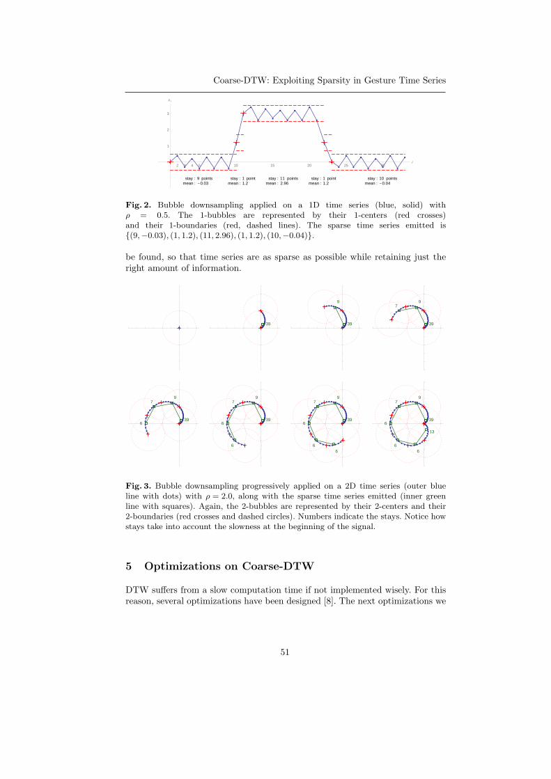
Coarse-DTW: Exploiting Sparsity in Gesture Time Series
2 3 4 5 10 15 20 25 30i
1
2
3
x i
stay : 9 points
mean : -0.03
stay : 1 point
mean : 1.2
stay : 11 points
mean : 2.96
stay : 1 point
mean : 1.2
stay : 10 points
mean : -0.04
Fig. 2. Bubble downsampling applied on a 1D time series (blue, solid) withρ = 0.5. The 1-bubbles are represented by their 1-centers (red crosses)and their 1-boundaries (red, dashed lines). The sparse time series emitted is(9,−0.03), (1, 1.2), (11, 2.96), (1, 1.2), (10,−0.04).
be found, so that time series are as sparse as possible while retaining just theright amount of information.
39 39
9
39
9
7
39
9
7
639
9
7
6
6
39
9
7
6
6
6
39
9
7
6
6
6
13
Fig. 3. Bubble downsampling progressively applied on a 2D time series (outer blueline with dots) with ρ = 2.0, along with the sparse time series emitted (inner greenline with squares). Again, the 2-bubbles are represented by their 2-centers and their2-boundaries (red crosses and dashed circles). Numbers indicate the stays. Notice howstays take into account the slowness at the beginning of the signal.
5 Optimizations on Coarse-DTW
DTW suffers from a slow computation time if not implemented wisely. For thisreason, several optimizations have been designed [8]. The next optimizations we
51

M. Dupont, P.-F. Marteau
considered are called lower bounds, designed to early-abandon computations ina k-Nearest Neighbor scenario.
The first lower bound LBKim [20] is transposable to Coarse-DTW: as with1D time series, the first and last pairs of points will always be matched togetheras long as the timeseries have each at least two points. First, the cost of match-ing the first points is: max(s1, t1).δ(v1, w1) because the first matching is donediagonally (A[0,1] = A[1,0] = ∞). Then, the cost of matching the last points ismin(sn, tm,max(sn, tm)) . δ(vn, wm). Hence, the lower bound is written:
Coarse-DTW(v, w) ≥ max(s1, t1).δ(v1, w1)+min(sn, tm,max(sn, tm)).δ(vn, wm)(2)
The second lower bound can be evaluated several times as DTW progresses:for any row i, the minimum of all cells A[i,.] is a lower bound to the DTW result.Indeed, this result is the last cell of the last row, and the sequence mapping a rowi to minj A[i,j] is increasing, because the costs are positive. Hence, during eachouter loop iteration (i.e., on index i), we can store the minimum of the currentrow and compare it to the best-so-far for possibly early abandoning. This canbe transposed directly to Coarse-DTW without additional modifications.
Finally, probably the most powerful lower bound for unidimensional time-series, known as LBKeogh [8], is based upon the calculation of an envelope; how-ever this calculation is not trivially transferable to the case of multidimensionaltime series simply by generalizing the uni-dimensional equations. Thus, we willunfortunately not consider it in our study.
6 Results
6.1 DTW vs. Coarse-DTW in 1-NN classification
We considered the classification accuracy and speed of three multidimensionallabeled time series datasets describing gesture movement. The classifier is 1-NNand we enabled all optimizations described earlier that apply to multidimensionaltime series, namely: LBKim and early abandoning on the minima of rows. Wereport only the classification time; learning time is zero because no processingis required. Each dataset is run once with DTW and several times with Coarse-DTW, each time with a different value for the downsampling radius ρ.
MSRAction3D [11] time series have 60 dimensions (twenty 3D joints) whichwe classified by cross-validating all 252 combinations of 5 actors in training and 5in test. uWaveGestureLibrary [XYZ] comes from the UCR time series database[6]; it can be considered as three independent uni-dimensional datasets, but werather used it here as a single set of 3-dimensional time series, which makes 1-NNDTW classification fall from 1D errors of respectively 27.3 %, 36.6 % and 34.2 %down to only 2.8 % as a 3D time series. Character Trajectories [19] comes fromthe UCI database and describes trajectories of character handwriting; they werefirst resampled to have all the same size (204 data points, size of the longestsequence in the dataset).
52

53

M. Dupont, P.-F. Marteau
References
1. Ghazi Al-Naymat, Sanjay Chawla, and Javid Taheri. Sparsedtw: A novel approachto speed up dynamic time warping. In Proceedings of the Eighth AustralasianData Mining Conference - Volume 101, AusDM ’09, pages 117–127, Darlinghurst,Australia, Australia, 2009. Australian Computer Society, Inc.
2. Kaushik Chakrabarti, Eamonn Keogh, Sharad Mehrotra, and Michael Pazzani.Locally adaptive dimensionality reduction for indexing large time series databases.ACM Trans. Database Syst., 27(2):188–228, June 2002.
3. L. Chen and R. Ng. On the marriage of lp-norm and edit distance. In Proceedingsof the 30th International Conference on Very Large Data Bases, pages 792–801,2004.
4. Selina Chu, Eamonn J. Keogh, David M. Hart, and Michael J. Pazzani. Iterativedeepening dynamic time warping for time series. In Robert L. Grossman, JiaweiHan, Vipin Kumar, Heikki Mannila, and Rajeev Motwani, editors, Proceedings ofthe Second SIAM International Conference on Data Mining, Arlington, VA, USA,April 11-13, 2002, pages 195–212. SIAM, 2002.
5. F. Itakura. Minimum prediction residual principle applied to speech recognition.Acoustics, Speech and Signal Processing, IEEE Transactions on, 23(1):67–72, Feb1975.
6. E. J. Keogh, X. Xi, L. Wei, and C.A. Ratanamahatana. The UCRtime series classification-clustering datasets, 2006. http://wwwcs.ucr.edu/ ea-monn/time series data/.
7. Eamonn Keogh, Kaushik Chakrabarti, Michael Pazzani, and Sharad Mehrotra.Dimensionality reduction for fast similarity search in large time series databases.JOURNAL OF KNOWLEDGE AND INFORMATION SYSTEMS, 3:263–286,2000.
8. Eamonn Keogh and Chotirat Ann Ratanamahatana. Exact indexing of dynamictime warping. Knowl. Inf. Syst., 7(3):358–386, March 2005.
9. Eamonn J. Keogh and Michael J. Pazzani. Scaling up dynamic time warping fordatamining applications. In Proceedings of the Sixth ACM SIGKDD InternationalConference on Knowledge Discovery and Data Mining, KDD ’00, pages 285–289,New York, NY, USA, 2000. ACM.
10. Daniel Lemire. Faster retrieval with a two-pass dynamic-time-warping lower bound.Pattern Recognition, 42(9):2169 – 2180, 2009.
11. W. Li, Z. Zhang, and Z. Liu. Action recognition based on a bag of 3d points. InIEEE CS Press, editor, Proc. IEEE Int’l Workshop on CVPR for Hum. Comm.Behav. Analysis, pages 9–14, 2010.
12. P. F. Marteau. Time warp edit distance with stiffness adjustment for time seriesmatching. IEEE Trans. Pattern Anal. Mach. Intell., 31(2):306–318, 2008.
13. Pranav Patel, Eamonn Keogh, Jessica Lin, and Stefano Lonardi. Mining motifs inmassive time series databases. In In Proceedings of IEEE International Conferenceon Data Mining (ICDM’02, pages 370–377, 2002.
14. H. Sakoe and S. Chiba. A dynamic programming approach to continuous speechrecognition. In Proceedings of the 7th International Congress of Acoustic, pages65–68, 1971.
15. Yasushi Sakurai, Masatoshi Yoshikawa, and Christos Faloutsos. Ftw: Fast similar-ity search under the time warping distance. In Proceedings of the Twenty-fourthACM SIGMOD-SIGACT-SIGART Symposium on Principles of Database Systems,PODS ’05, pages 326–337, New York, NY, USA, 2005. ACM.
54

Coarse-DTW: Exploiting Sparsity in Gesture Time Series
16. Stan Salvador and Philip Chan. Toward accurate dynamic time warping in lineartime and space. Intell. Data Anal., 11(5):561–580, October 2007.
17. Yutao Shou, Nikos Mamoulis, and David W. Cheung. Fast and exact warping oftime series using adaptive segmental approximations. Mach. Learn., 58(2-3):231–267, February 2005.
18. V. M. Velichko and N. G. Zagoruyko. Automatic recognition of 200 words. Inter-national Journal of Man-Machine Studies, 2:223–234, 1970.
19. Ben H Williams, Marc Toussaint, and Amos J Storkey. Extracting motion primi-tives from natural handwriting data. Springer, 2006.
20. Sang wook Kim, Sanghyun Park, and Wesley W. Chu. An index-based approachfor similarity search supporting time warping in large sequence databases. In InICDE, pages 607–614, 2001.
21. Byoung-Kee Yi and Christos Faloutsos. Fast time sequence indexing for arbitrarylp norms. In Proceedings of the 26th International Conference on Very Large DataBases, VLDB ’00, pages 385–394, San Francisco, CA, USA, 2000. Morgan Kauf-mann Publishers Inc.
55

56

Proceedings 1st International Workshop on Advanced Analytics and Learning on Temporal DataAALTD 2015
Preliminary Experimental Analysis of Reservoir
Computing Approach for Balance Assessment
Claudio Gallicchio1, Alessio Micheli1, Luca Pedrelli1, Federico Vozzi2, andOberdan Parodi2
1 Department of Computer Science, University of Pisa,Largo B. Pontecorvo 3, Pisa, Italy
2 IFC-CNR Pisa, Via Moruzzi 1, Pisa, Italy
Abstract. Evaluation of balance stability in elderly people is of promi-nent relevance in the field of health monitoring. Recently, the use of WiiBalance Board has been proposed as valid alternative to clinical balancetests, such as the widely used Berg Balance Scale (BBS) test, allowingto measure and analyze static features such as the duration or the speedof assessment of patients’ center of pressure. In an innovative way, inthis paper we propose to take into consideration the whole temporalinformation generated by the balance board, analyzing it by means ofdynamical neural networks. In particular, using Recurrent Neural Net-works implemented according to the Reservoir Computing paradigm, wepropose to estimate the BBS score from the temporal data generatedby the execution of one simple exercise on the balance board. Prelimi-nary experimental assessments of the proposed approach on a real-worlddataset show promising results.
Keywords: Reservoir Computing, Learning with Temporal Data, Bal-ance Assessment
1 Introduction
A sedentary lifestyle is a risk factor for the development of many chronic illnesses.The common physiological aging causes a decrease of global functional abilities:one of the most important is balance disorder [16]. The control of balance iscomplex, with a strong integration and coordination of multiple body elementsincluding visual, auditor and motor systems [9]. A comprehensive clinical as-sessment of balance is important for both diagnostic and therapeutic reasonsin clinical practice [4, 17]. The Berg Balance Scale (BBS) test is considered thegold standard assessment of balance with small intra-inter rater feasibility andgood internal validity. The work in [3] assessed the validity of the BBS by ex-amining how scale scores are related to clinical judgments, laboratory measuresof postural sway and external criteria reflecting balancing ability. Furthermore,scores could predict falls in the elderly, and how they are related to motor andfunctional performance in stroke patients. The Berg’s utility includes gradingdifferent patients’ balance abilities, monitoring functional balance over time andevaluating patients responses to different protocols of treatment [18]. Based ona test of 14 exercises/items, BBS is performance-based and has a scale of 0-4
Copyright c©2015 for this paper by its authors. Copying permitted for private and academicpurposes.
57

C. Gallicchio, A. Micheli, L. Pedrelli, F Vozzi, O. Parodi
(clinician assigned) score for each item, with a maximum overall score of 56.Within the scopes of the DOREMI European project (GA 611650), a technolog-ical platform to support and motivate older people to perform physical activityis under development, aiming at reducing sedentariness, cognitive decline andmalnutrition, promoting an improvement of quality of life and social inclusion.One of the element of DOREMI platform is a smart carpet, based on the use ofNintendo Wii Balance Board (WBB), able to gather information pertaining tousers’ weight distribution at the four corners of the board. Such tool allows todesign an automatic system for balance assessment through the daily repetitionof one simple BBS exercise. This type of analysis, done by users at medical fa-cilities or, remotely, at their own houses, can help clinicians in the evaluation ofolder people equilibrium and in control of its evolution.The use of the WBB is motivated by the fact that it represents a low-cost andportable tool, recently successfully adopted for problems related to standingposture correction [14] and for training standing balance in the elderly [19]. In-terestingly, the WBB has been validated in comparison with gold standard forceplatforms [13] in its reliability to track users’ balance parameters, such as the cen-ter of pressure path length and velocity [5]. However, it is worth to observe thatthe whole signal time-series generated by the WBB potentially contains a richerinformation than such static parameters. Thereby, in this paper we propose toanalyze the data generated by WBB using Recurrent Neural Networks (RNNs),which are learning models suitable for catching and processing dynamic knowl-edge from noisy temporal information. In particular, we considered the problemof estimating the BSS score of a patient using in input the temporal informa-tion generated by the execution of one simple BBS exercise on the WBB. Thisapproach potentially allows to avoid the need to repeat all the 14 BBS exercisesfor new patients. An alternative approach in [15] tries to estimate the BBS scoreof a patient using information extracted from a tri-axial accelerometer placed onthe lower back during the execution of some items of the BBS. Such approach,however, adopts a solution which is more intrusive for the patient. At the bestof our knowledge, our work represents the first attempt at estimating the BBSscore directly from the temporal data generated while the patient performs asimple balance exercise in an non-intrusive way using an external device.
2 Balance Assessment with RC
A measurement campaign has been conducted on 21 volunteers, aged between65 and 80 years. We measured the weight signal produced by the WBB at the 4corners of the board sampled at 5 Hz during the execution of the exercise # 10in the BBS test, i.e. turn to look behind, selected for its simple execution andshort duration (≈ 10 seconds). To take into account for possible variations in theexercise executions, for each patient we recorded data from a number of maxi-mum 10 repetitions of the exercise. We therefore obtained a Balance dataset fora regression task on sequences, containing couples of the type (s, ytg), where s isthe 4-dimensional input sequence of users’ weight values recorded by the WBB
58

Preliminary Experimental Analysis of RC for Balance Assessment
during the exercise and ytg is the target BBS score (over all the 14 exercises)of the corresponding patient, representing the ground-truth evaluated by a clin-ician during the campaign. For performance assessment we adopted the MeanAbsolute Error (MAE) of the BBS score estimation provided by the learningmodels. It is worth noticing that the Balance dataset contains an outlier patientwith BBS score of 24, which has been discarded for performance evaluation.We model the dynamics of the temporal data involved by the balance evaluationtask by dynamical neural networks models within the class of RNNs. In partic-ular, we adopt the Reservoir Computing (RC) approach [12] for RNN modeling,and take into consideration the Leaky Integration Echo State Network (LI-ESN)[11, 10], a state-of-the-art model for efficient learning in sequential/temporal do-mains, which has proved to be particularly suitable in dealing with the nature ofthe input data originated from sensors [1, 2]. LI-ESNs implement discrete timedynamical systems, and consist of two main components, a dynamical reservoir,which realizes a recurrent encoding of the input history and provides the systemwith a memory of the past [6], and a static readout which computes the output. ALI-ESN is composed of an input layer withNU units, a recurrent non-linear reser-voir layer with NR sparsely connected units, and a linear readout layer with NY
units. At each time step t, the reservoir computes a state x(t) ∈ RNR according
to a state transition function x(t) = (1−a)x(t−1)+a tanh(Winu(t)+Wx(t−1)),where u(t) ∈ R
NU is the input at time step t, Win ∈ RNR×NU is the input-to-
reservoir weight matrix, W ∈ RNR×NR is the recurrent reservoir weight matrix,
and a ∈ [0, 1] is the leaking rate parameter that controls the speed of the reservoirdynamics [11, 12]. For sequence-to-element regression tasks in which an outputvalue is required in correspondence of an entire input sequence, the use of a meanstate mapping function has proved to be effective [7, 8]. Accordingly, given aninput sequence of length n, s = [u(1), . . . ,u(n)], we average the state activationover the steps of the input sequence, i.e. χ(s) = 1
n
∑n
t=1 x(t). Then, the readoutis applied to compute the output of the model y(s) ∈ R
NY by a linear combina-tion of the elements in χ(s), i.e. y(s) = Woutχ(s), where Wout ∈ R
NY ×NR is thereadout-to-reservoir weight matrix. The readout is the only LI-ESN componentthat is trained, typically by efficient linear methods, e.g. pseudo-inversion andridge regression [12]. The reservoir is left untrained after initialization under theconstraints of the echo state property (ESP) [10, 12, 6]. A reservoir initialization
condition related to the spectral radius of W is often used in literature and isadopted in this paper, i.e. ρ((1− a)I+ aW)) < 1 (see e.g. [12, 6] for details).
3 Experimental Results
The experimental analysis presented in this paper aimed at preliminarily assess-ing the generalization performance of the proposed RC approach. At the sametime, in order to reduce the patients’ effort for future data gathering campaigns,we were also interested in empirically analyzing the trade-off between the numberof exercise repetitions for each patient required for training and the predictiveperformance that can be achieved. Accordingly, we took into consideration two
59

C. Gallicchio, A. Micheli, L. Pedrelli, F Vozzi, O. Parodi
experimental settings. In the first experimental setting, the Balance dataset wassplit in a training set, containing data from 17 patients (≈ 80% of the total), andan external test set for performance assessment, containing data from 4 patients(≈ 20% of the total, chosen in order to represent a uniform sampling in the rangeof possible BBS target values). We considered LI-ESNs with reservoir dimensionin NR ∈ 100, 200, 500, 10% of reservoir units connectivity, leaky parametera ∈ 0.1, 0.3, 0.5, 0.7, 1 and spectral radius ρ = 0.99. For each reservoir hyper-parametrization, we independently generated 5 reservoir guesses, averaging theresults over such guesses. For readout training we used pseudo-inversion andridge regression with regularization λr ∈ 10, 1, 0.7, 0.5, 0.3, 0.1, 0.01, 0.001. Thevalues of the reservoir hyper-parameters and readout regularization were chosenby model selection, adopting a 4-fold cross validation scheme over the trainingset. The selected LI-ESN resulted in a very good predictive performance, with atest MAE of 4.25±0.39, which outperforms the results in [15] for patients withina corresponding age range. Such results appear promising, also considering thetolerance in the ground-truth data due to human observations. Moreover, weobserved that the test error is higher for patients with lower BBS target scores,which correspond to a less sampled region in the input space.We also conducted a preliminary empirical investigation in order to evaluatehow the performance of the proposed LI-ESN approach scales with the numberof available training data for each patient. Accordingly, we uniformly split theBalance dataset into groups containing sequences pertaining to 3 patients each,according to a 7-fold cross validation scheme, progressively reducing the numberof training sequences for each patient. For this second experimental setting, werestricted to the case of LI-ESNs with NR = 100 reservoir units, whereas allthe others reservoir hyper-parameters and readout regularization values were se-lected (for each fold) on the validation set, considering the same range of valuesas in the case of the first experimental setting. Fig. 1 shows the MAE achievedby LI-ESNs on the validation set, for decreasing number of available training se-quences. Results show that the validation performance is approximately stablefor a number of training sequences per patient in the range of 10-4, while it getsrapidly worse as less than 4 training sequences per patient are used.
4 Conclusions
We have proposed an approach for assessing the balance abilities of elderly peo-ple based on RC networks, used for temporal processing of data recorded by aWBB during the execution of a simple BBS exercise, with the major advantageof automatically evaluating the BBS score using only 1 of the 14 exercises. Thepreliminary experimental analysis on a real-world dataset showed that our ap-proach is able to achieve a very good predictive performance, up to ≈ 4 pointsof discrepancy in the BBS score with respect to the gold standard, which is goodalso considering both the use of a single BBS item and the tolerance typical ofany subjective assessment scale. Overall, the possibility to infer the BBS scoreswith a good performance starting from the signal of a single BBS exercise shows
60

61

C. Gallicchio, A. Micheli, L. Pedrelli, F Vozzi, O. Parodi
cognitive ecology for smart homes. Journal of Intelligent & Robotic Systems pp.1–25 (2015)
2. Bacciu, D., Barsocchi, P., Chessa, S., Gallicchio, C., Micheli, A.: An experimentalcharacterization of reservoir computing in ambient assisted living applications.Neural Computing and Applications 24 (6), 1451–1464 (2014)
3. Berg, K.O., Wood-Dauphinee, S.L., Williams, J.I., Maki, B.: Measuring balance inthe elderly: validation of an instrument. Canadian journal of public health= Revuecanadienne de sante publique 83, S7–11 (1991)
4. Bloem, B.R., Visser, J.E., Allum, J.H.: Movement disorders - handbook of clinicalneurophysiology. Elsevier (2009)
5. Clark, R.A., Bryant, A.L., Pua, Y., McCrory, P., Bennell, K., Hunt, M.: Validityand reliability of the nintendo wii balance board for assessment of standing balance.Gait & posture 31(3), 307–310 (2010)
6. Gallicchio, C., Micheli, A.: Architectural and markovian factors of echo state net-works. Neural Networks 24(5), 440–456 (2011)
7. Gallicchio, C., Micheli, A.: Tree echo state networks. Neurocomputing 101, 319–337(2013)
8. Gallicchio, C., Micheli, A.: A preliminary application of echo state networks toemotion recognition. In: Proceedings of EVALITA 2014. pp. 116–119 (2014)
9. Horak, F.B., Wrisley, D.M., Frank, J.: The balance evaluation systems test(bestest) to differentiate balance deficits. Physical therapy 89(5), 484–498 (2003)
10. Jaeger, H., Haas, H.: Harnessing nonlinearity: Predicting chaotic systems and sav-ing energy in wireless communication. Science 304(5667), 78–80 (2004)
11. Jaeger, H., Lukosevicius, M., Popovici, D., Siewert, U.: Optimization and applica-tions of echo state networks with leaky-integrator neurons. Neural Networks 20(3),335–352 (2007)
12. Lukosevicius, M., Jaeger, H.: Reservoir computing approaches to recurrent neuralnetwork training. Computer Science Review 3(3), 127–149 (2009)
13. Maki, B.E., Holliday, P.J., Topper, A.K.: A prospective study of postural balanceand risk of falling in an ambulatory and independent elderly population. Journalof gerontology 49(2), M72–M84 (1994)
14. Shih, C.H., Shih, C.T., Chu, C.L.: Assisting people with multiple disabilitiesactively correct abnormal standing posture with a nintendo wii balance boardthrough controlling environmental stimulation. Research in developmental disabil-ities 31(4), 936–942 (2010)
15. Simila, H., Mantyjarvi, J., Merilahti, J., Lindholm, M., Ermes, M.: Accelerometry-based berg balance scale score estimation. Biomedical and Health Informatics,IEEE Journal of 18(4), 1114–1121 (2014)
16. Tinetti, M.E.: Performance-oriented assessment of mobility problems in elderlypatients. Journal of the American Geriatrics Society 34(2), 119–126 (1986)
17. Visser, J.E., Carpenter, M.G., van der Kooij, H., Bloem, B.R.: The clinical utilityof posturography. Clinical Neurophysiology 119(11), 2424–2436 (2008)
18. Wood-Dauphinee, S.L., Berg, K.O., Bravo, G.: The balance scale: Responding toclinically meaningful changes. Canadian journal of rehabilitation 10, 35–50 (1997)
19. Young, W., Ferguson, S., Brault, S., Craig, C.: Assessing and training standingbalance in older adults: a novel approach using the nintendo wiibalance board.Gait & posture 33(2), 303–305 (2011)
62

Proceedings 1st International Workshop on Advanced Analytics and Learning on Temporal DataAALTD 2015
Estimating Dynamic Graphical Models from
Multivariate Time-Series Data
Alexander J. Gibberd and James D.B. NelsonDepartment of Statistical Science, University College London, Gower Street, London,
WC1E 6BT
Abstract. We consider the problem of estimating dynamic graphical
models that describe the time-evolving conditional dependency struc-
ture between a set of data-streams. The bulk of work in such graphical
structure learning problems has focused in the stationary i.i.d setting.
However, when one introduces dynamics to such models we are forced to
make additional assumptions about how the estimated distributions may
vary over time. In order to examine the effect of such assumptions we
introduce two regularisation schemes that encourage piecewise constant
structure within Gaussian graphical models. This article reviews previ-
ous work in the field and gives an introduction to our current research.
1 Introduction
As the current data explosion continues, governments, business, and academiaare now not only harvesting more data points but also measuring an ever-increasing number of variables. The complex systems represented by such data-sets arise in many socio-scientific domains, such as: cyber-security, neurology,genetics and economics. In order to understand such systems, we must focus ouranalytic and experimental resources on investigating the most important rela-tionships. However, searching for significant relationships between variables is acomplex task. The number of possible graphs that encode such dependencies be-tween variables becomes exponentially large as the number of variables increase.Such computational issues are only compounded when such graphs vary overtime.
From a statistical estimation viewpoint, the significance of a model com-ponent can often be viewed in terms of a model selection problem. Generally,one may construct an estimate of model fit (a lower score implies better fit)L(M,θ,Y ), relating a given model M ∈ M and parameters θ ∈ Θ(M) to someobserved data Y ∈ Ω. Additionally, to account for differences in perceived modelcomplexity one should penalise this by a measure of complexity R(M,θ) (largeris more complex ). An optimal model and identification of parameters can befound through balancing the two terms, i.e:
(M, θ) = argminM∈M,θ∈Θ(M)
[
L(M,θ,Y ) +R(M,θ)]
. (1)
In statistics such a formulation is referred to as an M-estimator [15], however suchframeworks are popular across all walks of science [2], for example, maximum-likelihood (ML), least-squares, robust (Huber loss), penalised ML estimators can
Copyright c©2015 for this paper by its authors. Copying permitted for private and academicpurposes.
63

A.J. Gibberd, J.D.B. Nelson
all be discussed in this context. The principle idea is to suggest a mathemati-cal (and therefore can be communicated objectively) statement to the effect ofOccam’s Razor, whereby given similar model-fit, one should prefer the simplermodel. Depending on the specification of the functions L(·) and R(·) and asso-ciated model/parameter spaces, the problem in (1) can be either very easy ordifficult (for example, are the functions smooth, convex, etc).
In the next section we introduce the canonical Gaussian graphical model(GGM), and study the estimation of such models within the M-estimation frame-work. This lays the foundations for our proposed dynamical extensions. We con-clude with an example of an estimated dynamic GGM, some recovery propertiesof our estimators and discuss future research directions.
2 Gaussian graphical models
A Gaussian graphical model is a generative model which encodes the conditionaldependency structure between a set of P variables (Y1,...YP ) ∼ N (0,Σ) as agraph G(V,E). For now we will discuss the traditional i.i.d setting, in Section(4) we will demonstrate ways in which we may relax the assumption of thedistribution being identical over time.
In the standard case, the vertex set V = 1, . . . , P identifies variables andthe edge set E = (i, j), . . . (l,m) contains an edge if variables are condition-ally dependent, specifically if (i, j) 6∈ E we can decompose a joint distributionas P (Yi, Yj |YV \i,j) = P (Yi|YV \i,j)P (Yj |YV \i,j). The aim of our work is toestimate an edge-set that appropriately represents a given data-set. Within theGGM setting, learning such representations does not only provide insight by sug-gesting key dependencies, but also specifies a robust probabilistic model whichwe can use for tasks such as anomaly detection.
It is well known that the edges in a GGM are encoded by non-zero off-diagonal entries within the precision matrix Θ := Σ−1, specifically (i, j) ∈E ⇐⇒ Θi,j 6= 0 (see [12] for details). Learning the structure within the GGMcan then be linked with the general framework of (1) through a ML or Maximuma-posteriori (MAP) paradigm. Assuming T observations Y ∈ R
P×T drawn asi.i.d samples the model fit function L(·) can be related to the likelihood specifiedby the multivariate normal. Typically, one prefers to work with the log-likelihood,which if we assume µ = 0 (we assume this throughout) is given by:
log(P (Y |Θ))/T =1
2log det(Θ)−
1
2trace(SΘ)−
P
2ln(π) ,
where S = Y Y ⊤/T . Taking L(·) = − log det(Θ) + trace(SΘ) gives (in thesetting where T > P ) a well-behaved smooth, convex function describing howwell a given parameterisation Σ represents the data Y .
64

Estimating Dynamic Graphical Models from Multivariate Time-Series Data
3 Penalising complexity
If one considers Eq. (1) with the function R(·) = 0, i.e. no complexity penalty,
then the precision matrix estimator Θ := argminΘ0∈RP×P
[
− log det(Θ) +
trace(SΘ)]
demonstrates some undesirable properties indicative of over-fitting:
– The estimator exhibits large variance when T ≈ P and is very sensitive tochanges in observations leading to poor generalisation performance.
– In the high-dimensional setting (P > T ), the sample estimator is rank defi-cient (rank(S) < P ) and there is no unique estimator Θ.
In order to avoid estimating a complete GGM graph (where all vertices’s areconnected to each other), one must actively select edges according to some cri-teria. In the asymptotic setting where T ≫ P we can test for the significance ofedges by considering the asymptotic distribution of the empirical partial corre-
lation coefficients (ρij = −Θij/Θ1/2ii Θ
1/2jj ) [4]. However, such a procedure cannot
be performed in the high-dimensional setting (this is important for the dynam-ical extensions, see Sec. 4) as we require that the empirical estimate be positivesemi-definite.
An alternative approach to testing is to consider prior knowledge about thenumber of edges in the graph. If we assume a flat prior on the model M andparameters Θ(M), maximising the approximate posterior probability over mod-els P (M|Y ), then leads to the Bayesian information criterion for GGM [5]:
BIC(ΘML) = N(− log det(ΘML) + trace(SΘML)) + p log(N), where p is givenby the number of unique non-zeros within the ML estimated precision matrixΘML. Unfortunately, interpreting BIC under the framework in Eq. (1), we findthe complexity penalty R() = p log(N) is non-convex (p ∝ ‖Θ‖0 it basicallycounts the number of estimated edges). In order to arrive at a global minima an
exhaustive search over the model space (all possible graphs O(2P2
)) is required.
Alternatively, one can place an informative prior on the parameterisation andmodel (i.e. the GGM sparsity pattern) to encourage a parsimonious representa-tion. One popular approach [6,11,17,20] is to place a Laplace type prior on theprecision matrix in an effort to directly shrink off-diagonal values. Whilst onecould choose to perform full Bayesian inference for the posterior P (Θ|Y , γ) (asdemonstrated in [17]), a computationally less demanding approach is to performMAP estimation resulting in the graphical lasso problem [6]:
ΘGL := argminΘ≻0
[
− log det(Θ) + trace(SΘ) + (γ/N)‖Θ‖1]
, (2)
where ‖Θ‖1 =∑
1≤i,j≤P |Θi,j | is the ℓ1 norm of Θ. The graphical lasso problemcan yet again be interpreted within the general framework, except this time withR(·) = (γ/N)‖Θ‖1. Unlike BIC this complexity penalty is convex thus we canquickly find a global minima.
65

A.J. Gibberd, J.D.B. Nelson
4 Introducing dynamics
In this section we extend the basic GGM model to a dynamic setting wherebythe estimated graph is permitted to change as a function of time. Consider theP -variate time-series data Y ∈ R
P×T as before, however, we now permit thegenerative distribution to be a function of time, i.e:
(Y t1 , . . . Y
tP ) ∼ N (0,Σt) , (3)
the challenge is now to learn a GGM via (Σt)−1 for each time point t = 1, . . . , T .Clearly such a model is far more flexible than the identically distributed version,instead of O(P 2) parameters we now have O(P 2T ). In such a semi-parametricmodel the potential complexity can scale with the amount of data we haveavailable. Our aim is to harness this additional flexibility to identify potentialchanges within the graphical models which may shed insight onto dynamics ofthe data-generating system.
Local kernel/window estimation
Zhou et. al. [20] consider the dynamic GGM model in a continuous settingsuch that the underlying graphs are assumed to vary smoothly as a functionof time. To provide a local estimate of the covariance they suggest the estima-tor S(t) =
∑
s wstysy⊤s /
∑
s wst, where wst = K(|s− t|/hT ) are weights derivedfrom a symmetric non-negative kernel (typically one may use a box-car/Gaussianfunction) with bandwidth hT . The idea is that by replacing S with S(t) in thegraphical lasso problem (Eq. 2) it is possible to obtain a temporally localizedestimate of the graph Θ(t)GL. Given some smoothness conditions on the truecovariance matrices one can demonstrate [20] that the estimator is consistent
(estimator risk converges in probability R(Σ(t)) − R(Σ∗(t))P→ 0) even in the
dynamic (non-identically distributed) case.
Piecewise constant GGM
The seminal work by Zhou et al. [20] focused in the setting where graphs contin-uously and smoothly evolve over time. However, there are many situations wherewe might expect the smoothness assumptions to be broken. Our research [7,8,9]focuses on how we can incorporate different smoothness assumptions when esti-mating dynamic GGM. In particular we wish to study piecewise constant GGMwhere the generative distribution is strictly stationary within regions separatedby a set of changepoints T = τ1, . . . , τK, τi ∈ 1, . . . , T, such that:
P (Y t) = P (Y t+i) ∀ t, (t+ i) ∈ τk, . . . τk+1 for k = 0, . . . ,K − 1 .
If we keep the Gaussian assumption of Eq. (3), then estimation relates tofinding a set of K − 1 GGM describing the distribution between changepoints.Such a definition extends the usual definition of a changepoint [13] to multivari-ate distributions, it is expected that the number of changepoints should be smallrelative to the total period of measurement, i.e. K ≪ T and that such pointsmay lead to insight about changes within observed systems.
66

Estimating Dynamic Graphical Models from Multivariate Time-Series Data
5 Structure learning with dynamic GGM
Our approach to searching for changepoints falls naturally into the M-estimationframework of Eq. (1). As has already been discussed, appropriate complexitypenalties R(·) may act to induce sparsity in a given set of parameters. We proposetwo sparsity aware estimators that use such properties not only to estimate thegraphical model, but also jointly extract a sparse set of changepoints.
Independent Fusing
Our first approach (see [7,9], also related to [14,3,18]) constructs a model fit
function L(Θ,Y ) =∑T
t=1
(
− logdet(Θt) + tr(StΘt)
)
, where St= yt(yt)⊤/2 is
an estimate of the covariance for a specific time t. Clearly, there is not enough
information within Stto recover a graph, as we are effectively trying to estimate
with only one data point. To solve this problem we introduce an explicit prioron the smoothness of the graph via a complexity function
RIFGL(Θ) = λ1
T∑
t=1
‖Θt‖1 + λ2
T∑
t=2
‖Θt −Θt−1‖1 , (4)
where λ1, λ2 control the level of sparsity and number of changepoints in themodel. Unlike in the work of Zhou et al. our prior encodes an assumptionthat the model has a piecewise constant parameterisation (this is similar to thefused lasso, see [16,10]). We refer to the problem ΘTt=1 = argminΘ0
[
L(·) +
RIFGL(·)]
as defined above, as the independently fused graphical lasso (IFGL),it estimates changepoints at an individual edge level such that changepoints donot necessarily coincide between edges.
Group Fusing
Sometimes we have a-priori knowledge that particular variables may change in agrouped manner, that is changepoints across the edges which connect variablesmay coincide. Examples, might include genes associated with a specific biologicalfunction (see the example in Fig. 1), or stocks within a given asset class. In orderto encode such prior structure for changepoints one can adapt the smoothingprior to act over a group of edges, for such cases we suggest the group-fusedgraphical lasso (GFGL) penalty[9]:
RGFGL(Θ) = λ1
T∑
t=1
‖Θt‖1 + λ2
T∑
t=2
‖Θt −Θt−1‖2 . (5)
Optimisation
Both IFGL and GFGL form non-smooth convex optimisation problems whichcan be tackled within a variety of optimisation schemes. We have developed
67

68

Estimating Dynamic Graphical Models from Multivariate Time-Series Data
References
1. D. Angelosante and G. B. Giannakis. Sparse graphical modeling of piecewise-
stationary time series. IEEE International Conference on Acoustics, Speech andSignal Processing (ICASSP), 2011.
2. S. Boyd and L. Vandenberghe. Convex Optimization. 2004.
3. P. Danaher, P. Wang, and D. M. Witten. The joint graphical lasso for inverse co-
variance estimation across multiple classes. Journal of the Royal Statistical Society:Series B (Statistical Methodology), 2013.
4. M. Drton and M. D. Perlman. Model selection for Gaussian concentration graphs.
Biometrika, 2004.
5. R. Foygel and M. Drton. Extended Bayesian information criteria for gaussian
graphical models. In J.D. Lafferty, C.K.I. Williams, J. Shawe-Taylor, R.S. Zemel,
and A. Culotta, editors, Advances in Neural Information Processing Systems 23.2010.
6. J. Friedman, T. Hastie, and R. Tibshirani. Sparse inverse covariance estimation
with the graphical lasso. Biostatistics (Oxford, England), 2008.
7. A. J. Gibberd and J. D. B. Nelson. High dimensional changepoint detection with
a dynamic graphical lasso. IEEE International Conference on Acoustics, Speechand Signal Processing (ICASSP), 2014.
8. A. J. Gibberd and J. D. B. Nelson. Estimating multi-resolution dependency graphs
within a locally stationary wavelet framework. In review, 2015.
9. A. J. Gibberd and J. D. B. Nelson. Regularized Estimation of Piecewise Constant
Gaussian Graphical Models: The Group-Fused Graphical Lasso. In review, 2015.
10. Z. Harchaoui and C. Lévy-Leduc. Multiple change-point estimation with a total
variation penalty. Journal of the American Statistical Association, 2010.
11. J. Lafferty, H. Liu, and L. Wasserman. Sparse nonparametric graphical models.
Statistical Science, 2012.
12. S. L. Lauritzen. Graphical models. Oxford, 1996.
13. M. A. Little and N. S. Jones. Generalized methods and solvers for noise removal
from piecewise constant signals. II. New methods. Proceedings. Mathematical,physical, and engineering sciences / the Royal Society, 2011.
14. R. P. Monti, P. Hellyer, D. Sharp, R. Leech, C. Anagnostopoulos, and G. Montana.
Estimating time-varying brain connectivity networks from functional MRI time
series. NeuroImage, 2014.
15. S. N. Negahban, P. Ravikumar, M. J. Wainwright, and B. Yu. A unified framework
for high-dimensional analysis of M-estimators with decomposable regularizers. Sta-tistical Science, 2012.
16. R. Tibshirani, M. Saunders, S. Rosset, J. Zhu, and K. Knight. Sparsity and smooth-
ness via the fused lasso. Journal of the Royal Statistical Society: Series B (Statis-tical Methodology), 2005.
17. H. Wang. Bayesian graphical lasso models and efficient posterior computation.
Bayesian Analysis, 2012.
18. S. Yang, Z. Pan, X. Shen, P. Wonka, and J. Ye. Fused multiple graphical lasso.
Arxiv, 2012.
19. B. Zhang, J. Geng, and L. Lai. Multiple change-points estimation in linear regres-
sion models via sparse group lasso. IEEE Trans. Signal Processing, 2015.
20. S. Zhou, J. Lafferty, and L. Wasserman. Time varying undirected graphs. MachineLearning, 2010.
69

70

Proceedings 1st International Workshop on Advanced Analytics and Learning on Temporal DataAALTD 2015
Sequential Pattern Mining on Multimedia Data
Corentin Hardy, Laurent Amsaleg, Guillaume Gravier, Simon Malinowski, andReniniou
IRISA/Inria Rennes, France
Abstract. Analyzing multimedia data is a challenging problem due tothe quantity and complexity of such data. Mining for frequently recurringpatterns is a task often ran to help discovering the underlying structurehidden in the data. In this article, we propose audio data symbolizationand sequential pattern mining methods to extract patterns from audiostreams. Experiments show that this task is hard and that the symbol-ization is a critical step for extracting relevant audio patterns.
1 Introduction
The amount of multimedia data grows from day to day with ever increasingacquisition and storage capabilities. In turn, analyzing such complex data toextract knowledge is a challenging problem. For instance, analysts are lookingfor methods that could help to discover the underlying structure of multimediadocuments such as video or audio streams. Unsupervised extraction of recurrentpatterns and nding their occurrences in the data could provide such a seg-mentation and could achieve a rst step towards the automatic understandingof multimedia data. In an audio stream, a word, a jingle, or an advertisementcould typically represent a pattern. However, the variability of audio motifsmakes pattern mining dicult, especially audio motifs related to words, sincethe variability due to dierent speakers and channels is high.
Overall, the extraction of repeated motifs in time series is a very activedomain. Two kinds of approaches have been proposed: the rst one consists inworking directly with the time series and in nding close sub-sequences basedon a distance measure such as the Euclidean or the Dynamic Time Warping(DTW) [1] distances. The second one consists in transforming the time seriesinto sequences of symbols to then use sequential motif discovery algorithms [2].Very few works have investigated the second approach; this preliminary workthus explores how to use sequential pattern mining algorithms on audio data.
This paper is organized as follows. In Section 2, we review the related workabout motif discovery in audio data. In Section 3, we explain our proposedapproach. Section 4 presents preliminary results and section 5 concludes anddiscusses future issues for this work.
2 Related work
Motif discovery relies either on raw time series processing or on mining a symbolicversion [3,4,5]. In the rst kind of approaches, algorithms are mostly built on
Copyright c⃝2015 for this paper by its authors. Copying permitted for private and academicpurposes.
71

C. Hardy, L. Amsaleg, G. Gravier, S. Malinowski, R. Quiniou
the DTW distance which can deal with temporal distortions that often occursin audio signals [6]. Muscariello et al. [7] have proposed an extended version ofthe DTW for nding the best occurrence of a seed in a longer subsequence. Thiskind of approaches is ecient in terms of accuracy as the signal is completelyexploited but the computational cost of the DTW distance prevents its use onvery large databases.
Other approaches working with a symbolized version of the audio signalmostly use algorithms from bioinformatics to extract motifs. In [8], the MEMEalgorithm [9] is used to estimate a statistical model for each discovered motif.In [10], the SNAP algorithm [11] is used to search by query near-duplicate videosequences.
Some algorithms coming from bioinformatics are very ecient, but have beenoptimized to work with alphabets of very small size (from 4 to 20). In this paper,we consider the use of sequential pattern mining algorithms for discovering motifsin audio data.
3 Pattern mining on audio data
In this section, we explain how we used sequential pattern mining algorithmsto discover repeating patterns in audio data. As pattern mining algorithms dealwith symbolic sequences, we present rst how to transform time series related toaudio data into symbolic sequences. Then we show how to use sequential patternalgorithms on symbolic sequences.
MFCC (Mel-frequency cepstral coecients) is a popular method for repre-senting audio signals. First, MFCC coecients are extracted from the raw audiosignal (with a sliding window) yielding a 13-dimensional time series. Then, thismultivariate time series is transformed into a sequence of symbols. Many meth-ods have been proposed for transforming time series into a sequence of symbols.Here, we have chosen to use a method proposed by Wang et al. [12]. We havealso tried the very popular SAX approach [2]. SAX symbols contain very fewinformation about the original signal (only the average value on a window). Thissymbolisation technique is less adapted to our problem and produced worse re-sults.
To this end, each dimension of the 13-dimensional time series is divided intoconsecutive non-overlapping windows of length λ. The 13 sub-series related to thesame window are then concatenated (respecting the order of the MFCC data).The resulting vectors of size 13 × λ are then clustered by a k-means algorithmfor building a codebook, each word in the codebook corresponding to a cluster.Finally, the original multivariate time series is coded into a sequence of symbolsby assigning to each window the symbol in the codebook corresponding to theclosest cluster centroid. This symbolization process is sketched in Figures 1aand 1b.
The representation above could be too imprecise as it mixes coecients ofvery dierent order. To cope with this problem we propose to divide the 13dimensions into 2 or more sub-bands of consecutive dimensions that represent
72

Sequential Pattern Mining on Multimedia Data
(a) K-means clustering is performed onthe set of windows to build a codebook(of size 6, here).
(b) Every window is labeled by the sym-bol associated with the closest clustercentroid.
(c) Conversion of a 2 sub-band times series into a sequence of itemsets using 2 codebookof size 5.
Fig. 1: Time series symbolization into a sequence of items (gures 1a and 1b)and a sequence of itemsets (gure 1c).
more closely related dimensions. The same transformation described above op-erates on sub-bands and yields one codebook per sub-band. There are thus asmany symbolic sequences as there are sub-bands. Finally, the sub-band symbolsrelated to the same windows are grouped into itemsets in the Figure 1c.
Once the raw signal is transformed into a symbolic sequence of items oritemsets, classical sequential motif discovery algorithms can be applied. Twokinds of sequential pattern discovery algorithms have been proposed: algorithmsthat process sequences of items and algorithms that process sequences of itemsets(an itemset is a set of items that occur in a short time period). We have chosento evaluate one algorithm of each kind in this paper: MaxMotif [13] and CMP-Miner [14] that process respectively sequences of items and sequences of itemsets.
Note that, in the classical setting of sequential pattern mining, a pattern oc-currence may skip symbols in the sequence. For instance, acccb is an occurrenceof pattern ab in sequence dacccbe. Generally, algorithms provide means to putconstraints on extracted motifs, such as minimum and maximal motif lengthand the allowed gaps; gaps are symbols that can be skipped when looking for apattern occurrence. In our application, it is crucial to allow gaps in motifs sincetemporal distortions often occurs in audio signals.
MaxMotif enumerates all frequent (with respect to a given minimal support)closed patterns in a database of item sequences. MaxMotif allows gaps in the
73
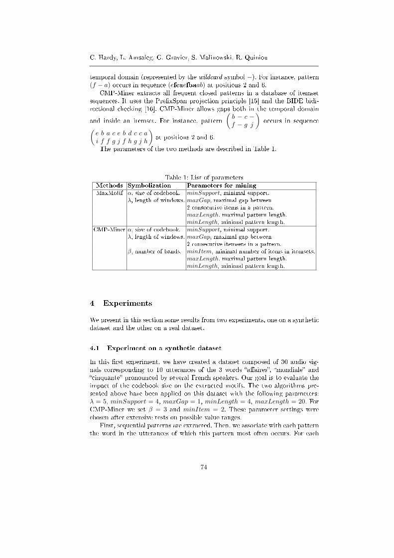
C. Hardy, L. Amsaleg, G. Gravier, S. Malinowski, R. Quiniou
temporal domain (represented by the wildcard symbol −). For instance, pattern(f − a) occurs in sequence (efcaefbaab) at positions 2 and 6.
CMP-Miner extracts all frequent closed patterns in a database of itemsetsequences. It uses the PrexSpan projection principle [15] and the BIDE bidi-rectional checking [16]. CMP-Miner allows gaps both in the temporal domain
and inside an itemset. For instance, pattern
(b − c −f − g j
)occurs in sequence(
e b a c e b d c c ai f f g j f h g j h
)at positions 2 and 6.
The parameters of the two methods are described in Table 1.
Table 1: List of parametersMethods Symbolization Parameters for mining
MaxMotif α, size of codebook. minSupport, minimal support.λ, length of windows. maxGap, maximal gap between
2 consecutive items in a pattern.maxLength, maximal pattern length.minLength, minimal pattern length.
CMP-Miner α, size of codebook. minSupport, minimal support.λ, length of windows. maxGap, maximal gap between
2 consecutive itemsets in a pattern.β, number of bands. minItem, minimal number of items in itemsets.
maxLength, maximal pattern length.minLength, minimal pattern length.
4 Experiments
We present in this section some results from two experiments, one on a syntheticdataset and the other on a real dataset.
4.1 Experiment on a synthetic dataset
In this rst experiment, we have created a dataset composed of 30 audio sig-nals corresponding to 10 utterances of the 3 words aaires, mondiale andcinquante pronounced by several French speakers. Our goal is to evaluate theimpact of the codebook size on the extracted motifs. The two algorithms pre-sented above have been applied on this dataset with the following parameters:λ = 5, minSupport = 4, maxGap = 1, minLength = 4, maxLength = 20. ForCMP-Miner we set β = 3 and minItem = 2. These parameter settings werechosen after extensive tests on possible value ranges.
First, sequential patterns are extracted. Then, we associate with each patternthe word in the utterances of which this pattern most often occurs. For each
74

Sequential Pattern Mining on Multimedia Data
extracted pattern, a precision/recall score is computed. Figure 2a and 2b depictthe precision/recall score versus the codebook size for MaxMotif and CMP-Miner. As can be seen, MaxMotif obtains the best eciency. This gure alsoshows that when the codebook size increases, the precision improves slightly butnot the recall.
Figure 2c shows the pattern length distribution for dierent codebook sizesfor MaxMotif. For small codebooks, many long patterns are extracted. How-ever, they are not very accurate because, being general, they can occur in manydierent sequences. For big codebooks, many pattern candidates can be found,reecting sequence variability. However, many candidates have a low support,often under the minimal threshold, and, so, less patterns are extracted.
The symbolization step is crucial. Figure 2d shows ve symbolic representa-tions of the word cinquante for a codebook of size 15. These strings highlightthe two kinds of variability (spectral and temporal) that makes the task hard formining algorithms in this example. The same experiment was performed usingthe SAX symbolization method [2] on each dimension of the multidimensionaltimes series. This representation revealed to be less accurate. Indeed, the resultsobtained by CMP-Miner using the SAX representation were worse. There is nospace to detail these results here.
4.2 Experiment on a larger database
Now, we consider a dataset containing 7 hours of audio content. The dataset isdivided into 21 audio tracks coming from various radio stations. This experienceis closer to a real setting.
Only MaxMotif has been tested on this dataset. The parameters were: λ = 4,α = 80, minSupport = 40, maxGap = 1, minLength = 5, maxLength = 20.The codebook size is greater than in the previous experiment to deal with moredierent sounds. Pattern extraction is very fast: less than 4 minutes for morethan one million of patterns. Some of them are interesting and correspond, forinstance, to crowd noises, jingle and music patterns or short silence. However,similarly to the experiment on the synthetic dataset, only very few patternscorresponding to repeated words could be extracted.
5 Conclusion
In this paper, we have presented a preliminary work investigating how to usesequential pattern mining algorithms for audio data. The aim of this work wasto evaluate whether these algorithms could be relevant for this problem. Theexperiments pointed out the diculty to mine audio signals, because of temporaland spectral distortion. Same words pronounced in dierent contexts and bydierent speakers can be very dierent and yield very dierent patterns. Theresults are promising but both symbolization and motif extraction should beimproved. For instance, to account for spectral variability, considering distancesbetween symbols should improve the overall performance of pattern extraction.
75

C. Hardy, L. Amsaleg, G. Gravier, S. Malinowski, R. Quiniou
(a) Precision/Recall curves for MaxMotif. (b) Precision/Recall curves for CMP-Minerwith 3 sub-bands.
(c) Pattern size distribution for dierentsize of codebook.
(d) Example of representation fora codebook of size 15.
Fig. 2: Results of experience on synthetic data.
We have also noticed that all the dimensions of the MFCC times series arenot as important for the discovery. Selecting or weighting the dimensions ofmultidimensional time series could improve the performance too.
References
1. A. Mueen, Enumeration of time series motifs of all lengths, in Data Mining(ICDM), 2013 IEEE 13th International Conference on, pp. 547556, Dec 2013.
2. J. Lin, E. Keogh, L. Wei, and S. Lonardi, Experiencing sax: A novel symbolicrepresentation of time series, Data Min. Knowl. Discov., vol. 15, pp. 107144,Oct. 2007.
3. C. Herley, ARGOS: Automatically extracting repeating objects from multimediastreams, IEEE Trans. on Multimedia, vol. 8, pp. 115129, Feb. 2006.
4. P. Esling and C. Agon, Time-series data mining, ACM Computing Surveys(CSUR), vol. 45, no. 1, p. 12, 2012.
5. C. H. Mooney and J. F. Roddick, Sequential pattern mining approaches andalgorithms, ACM Comput. Surv., vol. 45, Mar. 2013.
76

Sequential Pattern Mining on Multimedia Data
6. A. Park and J. R. Glass, Unsupervised pattern discovery in speech, IEEE Trans-action on Acoustic, Speech and Language Processing, vol. 16, pp. 186197, Jan.2008.
7. A. Muscariello, G. Gravier, and F. Bimbot, Audio keyword extraction by unsu-pervised word discovery, in INTERSPEECH 2009: 10th Annual Conference of theInternational Speech Communication Association, (Brighton, United Kingdom),Sept. 2009.
8. J. J. Burred, Genetic motif discovery applied to audio analysis, in InternationalConference on Acoustics, Speech and Signal Processing, pp. 361364, IEEE, 2012.
9. T. Bailey and C. Elkan, Unsupervised learning of multiple motifs in biopolymersusing expectation maximization, Machine Learning, vol. 21, no. 1-2, pp. 5180,1995.
10. L. S. d. Oliveira, Z. K. do Patrocinio, S. J. F. Guimarães, and G. Gravier, Searchingfor near-duplicate video sequences from a scalable sequence aligner, in Interna-tional Symposium on Multimedia, pp. 223226, IEEE, 2013.
11. M. Zaharia, W. J. Bolosky, K. Curtis, A. Fox, D. Patterson, S. Shenker, I. Stoica,R. M. Karp, and T. Sittler, Faster and more accurate sequence alignment withsnap, arXiv preprint arXiv:1111.5572, 2011.
12. Q. Wang, V. Megalooikonomou, and C. Faloutsos, Time series analysis with mul-tiple resolutions, Information Systems, vol. 35, no. 1, pp. 5674, 2010.
13. H. Arimura and T. Uno, An ecient polynomial space and polynomial delay algo-rithm for enumeration of maximal motifs in a sequence, Journal of CombinatorialOptimization, vol. 13, 2007.
14. A. J. Lee, H.-W.Wu, T.-Y. Lee, Y.-H. Liu, and K.-T. Chen, Mining closed patternsin multi-sequence time-series databases, Data & Knowledge Engineering, vol. 68,no. 10, pp. 1071 1090, 2009.
15. J. Pei, J. Han, B. Mortazavi-Asl, H. Pinto, Q. Chen, U. Dayal, and M.-C. Hsu, Pre-xspan: Mining sequential patterns eciently by prex-projected pattern growth,in International Conference on Data Engineering, p. 0215, 2001.
16. J. Wang and J. Han, Bide: ecient mining of frequent closed sequences, inData Engineering, Proceedings. 20th International Conference on Data Engineer-ing, pp. 7990, March 2004.
77

78

Proceedings 1st International Workshop on Advanced Analytics and Learning on Temporal DataAALTD 2015
Time Series Classification in Dissimilarity Spaces
Brijnesh J. Jain and Stephan SpiegelBerlin Institute of Technology, Germany
[email protected], [email protected]
Abstract. Time series classification in the dissimilarity space combinesthe advantages of the dynamic time warping and the rich mathematicalstructure of Euclidean spaces. We applied dimension reduction usingPCA followed by support vector learning on dissimilarity representationsto 43 UCR datasets. Results indicate that time series classification indissimilarity space has potential to complement the state-of-the-art.
1 Introduction
Time series classification finds many applications in diverse domains such asspeech recognition, medical signal analysis, and recognition of gestures [2–4].Surprisingly, the simple nearest-neighbor method together with the dynamictime warping (DTW) distance still belongs to the state-of-the-art and is reportedto be exceptionally difficult to beat [1, 5, 10]. This finding is in stark contrast toclassification in Euclidean spaces, where nearest neighbor methods often merelyserve as baseline. One reason for this situation is that nearest neighbor methodsin Euclidean spaces compete against a plethora of powerful statistical learningmethods. The majority of these statistical learning methods are based on theconcept of derivative not available for warping-invariant functions on time series.
The dissimilarity space approach proposed by [7] offers to combine the advan-tages of the DTW distance with the rich mathematical structure of Euclideanspaces. The basic idea is to first select a set of k reference time series, calledprototypes. Then the dissimilarity representation of a time series consists of kfeatures, each of which represents its DTW distance from one of the k proto-types. Since dissimilarity representations are vectors from R
k, we can resort tothe whole arsenal of mathematical tools for statistical data analysis. The dis-similarity space approach has been systematically applied to the graph domainusing graph matching [6, 9]. A similar systematic study of the dissimilarity spaceapproach for time series endowed with the DTW distance is still missing.
This paper is a first step towards exploring the dissimilarity space approachfor time series under DTW. We hypothesize that combining the advantages ofboth, the DTW distance and statistical pattern recognition methods, can resultin powerful classifiers that may complement the state-of-the-art. The proposedapproach applies principal component analysis (PCA) for dimension reduction ofthe dissimilarity representations followed by training a support vector machine(SVM). Experimental results provide support for our hypothesis.
Copyright c©2015 for this paper by its authors. Copying permitted for private and academicpurposes.
79

B. Jain, S. Spiegel
2 Dissimilarity Representations of Time Series
2.1 Dynamic Time Warping Distance
A time series of length n is an ordered sequence x = (x1, . . . , xn) with featuresxi ∈ R sampled at discrete points of time i ∈ [n] = 1, . . . , n. To define theDTW distance between time series x and y of length n and m, resp., we constructa grid G = [n] × [m]. A warping path in grid G is a sequence φ = (t1, . . . , tp)consisting of points tk = (ik, jk) ∈ G such that
1. t1 = (1, 1) and tp = (n,m) (boundary conditions)2. tk+1 − tk ∈ (1, 0), (0, 1), (1, 1) (warping conditions)
for all 1 ≤ k < p. The cost of warping x = (x1, . . . , xn) and y = (y1, . . . , ym)along φ is defined by
dφ(x,y) =∑
(i,j)∈φ
(xi − yj)2,
where (xi − yj)2
is the local transformation cost of assigning features xi to yj .Then the distance function
d(x,y) = minφ
dφ(x,y),
is the dynamic time warping (DTW) distance between x and y, where the min-imum is taken over all warping paths in G.
2.2 Dissimilarity Representations
Let (T , d) be a time series space T endowed with the DTW distance d. Supposethat we are given a subset
P = p1, . . . ,pk ⊆ T
of k reference time series pi ∈ T , called prototypes henceforth. The set P ofprototypes gives rise to a function of the form
φ : T → Rk, x 7→ (d(x,p1), . . . , d(x,pk)),
where Rk is the dissimilarity space of (T , d) with respect to P. The k-dimensionalvector φ(x) is the dissimilarity representation of x. The i-th feature of φ(x)represents the dissimilarity d(x,pi) between x and the i-th prototype pi.
2.3 Learning Classifiers in Dissimilarity Space
Suppose thatX = (x1, y1), . . . , (xn, yn) ⊆ T × Y.
is a training set consisting of n time series xi with corresponding class labelsyi ∈ Y. Learning in dissimilarity space proceeds in three steps: (1) select a
80

Learning in Dissimilarity Spaces
suitable set of prototypes P on the basis of the training set D, (2) embed timeseries into the dissimilarity space by means of their dissimilarity representations,and (3) learn a classifier in the dissimilarity space according to the empirical riskminimization principle.
The performance of a classifier learned in dissimilarity spaces crucially de-pends on a proper dissimilarity representation of the time series. We distinguishbetween two common approaches:
1. Prototype selection: construct a set of prototypes P from the training set X .2. Dimension reduction: perform dimension reduction in the dissimilarity space.
There are numerous strategies for prototype selection. Naive examples in-clude all elements of the training set X and sampling a random subset of X . Formore sophisticated selection methods, we refer to [8]. Dimension reduction ofthe dissimilarity representation includes methods such as, for example, principalcomponent analysis (PCA).
3 Experiments
The goal of this experiment is to assess the performance of the following classifiersin dissimilarity space: (1) nearest neighbor using the Euclidean distance (ED-DS), (2) support vector machine (SVM), and (3) principal component analysis ondissimilarity representations followed by support vector machine (PCA+SVM).
3.1 Experimental Protocol
We considered 43 datasets from the UCR time series datasets [4], each of whichcomes with a pre-defined training and test set. For each dataset we used thewhole training set as prototype set. To embed the training and test examplesinto a dissimilarity space, we computed their DTW distances to the prototypes.
We trained all SVMs with RBF-kernel using the embedded training examples.We selected the parameters γ and C of the RBF-kernel over a two-dimensionalgrid with points (γi, Cj) = (2i, 2j), where i, j are 30 equidistant values from[−10, 10]. For each parameter configuration (γi, Cj) we performed 10-fold cross-validation and selected the parameters (γ∗, C∗) with the lowest average classi-fication error. Then we trained the SVM on the whole embedded training setusing the selected parameters (γ∗, C∗). Finally, we applied the learned model tothe embedded test examples for estimating the generalization performance.
For PCA+SVM we performed dimension reduction using PCA prior trainingof the SVM. We considered the q first dimensions with highest variance, whereq ∈ 1, 1 + a, 1 + 2a, . . . . , 1 + 19a with a being the closest integer of k/20 andk is the dimension of the dissimilarity space. For each q, we performed hyper-parameter selection for the SVM as described above. We selected the parameterconfiguration (q∗, γ∗, C∗) that gave the lowest classification error. Then we ap-plied PCA on the whole embedded training set, retained the first q∗ dimensionsand trained the SVM on the embedded training set after dimension reduction.
81

82

Learning in Dissimilarity Spaces
Data DTW ED-DS SVM PCA+SVM
50words 31.0 42.9 33.4 31.0 (+0.0)Adiac 39.6 40.2 34.0 37.6 (+5.1)Beef 50.0 56.7 60.0 40.0 (+20.0)CBF 0.3 0.2 1.4 0.2 (+32.7)ChlorineConcentration 35.2 48.3 28.9 30.2 (+14.3)CinC ECG Torso 34.9 44.0 41.4 39.8 (-14.0)Coffee 17.9 39.3 32.1 17.9 (+0.0)Cricket X 22.3 38.5 24.1 23.6 (-5.8)Cricket Y 20.8 37.9 20.0 19.7 (+5.1)Cricket Z 20.8 34.9 20.8 18.2 (+12.5)DiatomSizeReduction 3.3 4.2 10.8 13.7 (-315.9)ECG 23.0 20.0 16.0 18.0 (+21.7)ECGFiveDays 23.2 22.4 24.9 14.1 (+39.4)Face (all) 19.2 28.9 23.8 10.9 (+43.0)Face (four) 17.1 19.3 13.6 17.0 (+0.0)FacesUCR 9.5 17.1 13.4 9.0 (+5.6)Fish 16.7 32.6 17.7 14.3 (+14.5)Gun-Point 9.3 20.0 6.7 8.7 (+7.1)Haptics 62.3 58.4 54.9 54.9 (+11.9)InlineSkate 61.6 61.8 65.5 68.4 (-11.0)ItalyPowerDemand 5.0 8.4 6.5 6.3 (-26.3)Lighting 2 13.1 18.0 14.8 16.4 (-25.1)Lighting 7 27.4 37.0 23.3 20.5 (+25.0)Mallat 6.6 4.6 5.6 5.5 (+17.3)Medical Images 26.3 27.9 24.9 21.7 (+17.4)MoteStrain 16.5 24.8 17.2 14.1 (+14.8)Olive Oil 13.3 13.3 10.0 13.3 (+0.0)OSU Leaf 40.9 45.0 36.0 38.0 (+7.1)SonyAIBORobotSurface 27.5 16.3 22.3 6.7 (+75.8)SonyAIBORobotSurface II 16.9 19.4 17.4 19.3 (-14.2)Swedish Leaf 21.0 27.2 14.4 18.7 (+10.9)Symbols 5.0 5.3 8.7 5.3 (-6.5)Synthetic Control 0.7 1.7 1.3 2.0 (-185.7)Trace 0.0 1.0 1.0 0.0 (+0.0)TwoLeadECG 9.6 18.7 7.7 7.1 (+25.9)TwoPatterns 0.0 18.7 0.0 0.0 (+0.0uWaveGestureLibrary X 27.3 28.9 20.8 20.6 (+24.6)uWaveGestureLibrary Y 36.6 40.5 28.6 28.5 (+22.2)uWaveGestureLibrary Z 34.2 34.6 27.0 26.9 (+21.4)Wafer 2.0 1.5 1.1 1.5 (+26.2)WordsSynonyms 35.1 43.9 39.0 34.3 (+2.2)yoga 16.4 20.0 14.0 14.8 (+9.6)
Table 1. Error rates in percentages. Numbers in parentheses show percentage improve-ment of PCA+SVM with respect to DTW.
results, the improvements are only small and could also be occurred by chancedue to the random sampling of the training and test set.
The second observation to be made is that the SVM using all prototypescomplements NN+DTW. Better and worse predictive performance of both clas-sifiers is balanced. This shows that powerful learning algorithms can partiallycompensate for poor representations.
83

B. Jain, S. Spiegel
The third observation to be made is that SVM+PCA outperformed all otherclassifiers. Furthermore, SVM+PCA is better than NN+DTW in 28 and worsein 9 out of 42 cases. By reducing the dimension using PCA, we obtain betterdissimilarity representations for classification. Table 1 highlights relative im-provements and declines of PCA+SVM compared to NN+DTW with ±10% ormore in blue and red color, respectively. We observe a relative change of at least±10% in 27 out of 43 cases. This finding supports our hypothesis that learningon dissimilarity representations complements NN+DTW.
4 Conclusion
This paper is a first step to explore dissimilarity space learning for time seriesclassification under DTW. Results combining PCA with SVM on dissimilarityrepresentations are promising and complement nearest neighbor methods us-ing DTW in time series spaces. Future work aims at exploring further elasticdistances, prototype selection, dimension reduction, and learning methods.
References
1. G.E. Batista, X. Wang, and E.J. Keogh. A Complexity-Invariant Distance Measurefor Time Series. SIAM International Conference on Data Mining, 11:699–710, 2011.
2. T. Fu. A review on time series data mining. Engineering Applications of Artificial
Intelligence, 24(1):164–181, 2011.3. P. Geurts. Pattern extraction for time series classification. Principles of Data Mining
and Knowledge Discovery, pp. 115–127, 2001.4. E. Keogh, Q. Zhu, B. Hu, Y. Hao., X. Xi, L. Wei, and C. A. Ratanamahatana. The
UCR Time Series Classification/Clustering Homepage: www.cs.ucr.edu/~eamonn/
time_series_data/, 2011.5. J. Lines and A. Bagnall. Time series classification with ensembles of elastic distance
measures. Data Mining and Knowledge Discovery, 2014.6. L. Livi, A. Rizzi, and A. Sadeghian. Optimized dissimilarity space embedding for
labeled graphs. Information Sciences, 266:47–64, 2014.7. E. Pekalska and R.P.W. Duin The Dissimilarity Representation for Pattern Recog-
nition. World Scientific Publishing Co., Inc., 2005.8. E. Pekalska, R.P.W. Duin, and P. Paclik. Prototype selection for dissimilarity-based
classifiers. Pattern Recognition, 39(2): 189–208, 2006.9. K. Riesen and H. Bunke. Graph classification based on vector space embedding.
International Journal of Pattern Recognition and Artificial Intelligence, 23(6):1053–1081, 2009.
10. X. Xi, E. Keogh, C. Shelton, L. Wei, and C.A. Ratanamahatana. Fast time se-ries classification using numerosity reduction. International Conference on Machine
Learning, pp. 1033–1040, 2006.
84

Proceedings 1st International Workshop on Advanced Analytics and Learning on Temporal DataAALTD 2015
Temporal Density Extrapolation
Georg KremplKnowledge Management & Discovery
Otto-von-Guericke University MagdeburgUniversitatsplatz 2, 39106 Magdeburg, Germany
https://kmd.cs.ovgu.de/res/driftmining
Abstract. Mining evolving datastreams raises the question how to ex-trapolate trends in the evolution of densities over time. While approachesfor change diagnosis work well for interpolating spatio-temporal den-sities, they are not designed for extrapolation tasks. This work stud-ies the temporal density extrapolation problem and sketches two ap-proaches that addresses it. Both use a set of pseudo-points in combina-tion with spatio-temporal kernel density estimation. The first, weight-extrapolating approach, uses regression on the weights of stationary-located pseudo-points. The second, location-extrapolating approach, ex-trapolates the trajectory of uniformly-weighted pseudo-points within thefeature space.
Keywords: kernel density estimation, density extrapolation, densityforecasting, spatio-temporal density, evolving datastreams, nonstation-ary environments, concept drift, drift mining
1 Introduction
Density estimation methods, like kernel density estimation [14, 13], allow to learna model from instances observed at different positions in feature space, andto use this model to estimate the density at any position within this featurespace. While the original work in [14, 13] is limited to spatial densities of astationary distribution, the approach was extended for spatio-temporal densityestimation of non-stationary distributions in [1, 2]. This so-called velocity densityestimation allows to estimate and visualise trends in densities. However, theseexisting approaches are not directly applicable for predicting the density at futuretime points, for example to extrapolate trends in the evolution of densities andfor building classifiers that work with delayed label information [10, 5]. Suchtemporal density extrapolation should predict the densities at spatio-temporalcoordinates in the future, given a sample of (historic) instances observed atdifferent positions in feature space and at different times in the past.
We propose and study two approaches to address this problem. Both useextrapolation of pseudo-points in combination with spatio-temporal kernel den-sity estimation. The first approach extrapolates the weights of stationary locatedpseudo-points, while the second extrapolates the path of moving pseudo-points offixed weight. Subsequently, these weight- or position-extrapolated pseudo-pointsare used in a spatio-temporal kernel density estimation.
Copyright©2015 for this paper by its authors. Copying permitted for private and academicpurposes.
85

G. Krempl
In the following Section 2, we review the related work, before sketching thetwo approaches in Section 3 and concluding in Section 4.
2 Related Work
The task of estimating the probability density based on a sample of indepen-dently and identically distributed (iid) observations has been intensively studied.Density estimation methods, like kernel density estimation [14, 13], allow to learna model from instances observed at different positions in feature space, and touse this model to estimate the density at any position within this feature space.The difficulties of the early kernel and near-neighbour density estimation tech-niques when extended to multivariate settings was addressed by approaches likeprojection pursuit density estimation, proposed in [4]. All these density estima-tion approaches, as well as related curve regression approaches, require an iidsample from a stationary distribution [11].
In the case of a nonstationary distribution, one might be interested in esti-mating the density at different points in time and space. In [1, 2], this problemof spatio-temporal density estimation is addressed by combining spatial kerneldensity estimation with a temporal weighting of instances. A framework for so-called change diagnosis in evolving datastreams is proposed, which estimatesthe rate of change at each region by using a user-specified temporal window tocalculate forward and reverse time slice density estimates. This velocity den-sity estimation technique is applicable for spatio-temporal density interpolation,for monitoring and visualising the change of densities in a (past) time window.However, it is not designed for extrapolating the density to (future) time pointsoutside the window of observed historical data.
Related to change diagnosis is change mining [3], which aims to understandthe changes in data distributions themselves. Within this paradigm, the ideaof so-called drift-mining approaches [8, 9, 5] is to model the evolution of distri-butions in order to extrapolate them to future time points, thereby addressingproblems of verification latency or label delay. The algorithm APT proposed in[8] uses matching between labelled old and unlabelled new instances to infer thelabels of the later, thus indirectly estimating the class-conditional distributionsof the new instances. Likewise, an expectation-maximisation approach is used in[9] to track components of a Gaussian mixture model over time. In [5], a mix-ture model is learned on old labelled data and compared to density estimateson current unlabelled data, thereby inferring changes such as of the class prior.However, these approaches are again not designed for directly extrapolating den-sities.
Density forecasting approaches [15, 16, 7], on the other hand, focus on theprediction of a single variable’s (mostly unimodal) density at a particular futuretimepoint, based on an observed time series of this variable’s values. In the sim-plest case, as discussed for example in [16], this is done by providing a confidenceinterval for a point estimate, obtained by assuming a particular distribution ofthis variable. More sophisticated approaches return (potentially multi-modal)
86

Temporal Density Extrapolation
density estimates by combining several predictions, which are obtained for ex-ample by different macroeconomic models, experts, or simulation outcomes, intoa distribution estimation by kernel methods. Nevertheless, their multi-modalcharacter originates from the different modes in the combined unimodal mod-els. In addition, most works consider only a single variable. One exception is[7], where univariate forecasts of two explanatory variables are converted usingconditional kernel density estimation into forecasts of the dependent variable.
In contrast to density forecasting above, we are concerned with temporaldensity extrapolation of a potentially multi-modal density distribution. Further-more, instead of having a time series of single observations at any one time,our input data consists of multiple observations at any one time. This temporal
density extrapolation is related to spatial density extrapolation [17, 6], which ad-dresses the extrapolation of densities for feature values that have not been seenyet in historical instances. In [17], the authors suggest a Taylor series expansionabout the point of interest to estimate the density, while in [6] a statistical testis provided to examine whether the data distribution is distinct from a uniformdistribution at the extrapolation position. While modelling time as a feature ispossible, there is an important difference in extrapolation between time and fea-ture space: one expects the density to diminish towards unpopulated (and thusunseen) positions in feature space. However, there is no a priori reason to assumedensities to decrease towards yet unseen moments in time. On the contrary, itis reasonable to assume that at each point in time (whether future, current, orpast) the density integrates to one over the feature space.
3 Temporal Density Extrapolation
To address the problem of extrapolating the observed, potentially multi-modaldensity-distribution of instances to future time points, we propose an approachbased on pseudo-points. These pseudo-points are used in the spatio-temporal ker-nel density estimation in lieu of the originally observed instances. The resultingkernel density estimation model can be interpreted as a mixture model, whereeach pseudo-point constitutes itself a component. The pseudo-points evolve overtime, either by changing their weight (their component’s mixing proportion), orby changing their position (their component’s location). Therefore, the learningtask is to fit a trend function to the evolution of each pseudo-point. We presenteach of the two variants in the next Subsections 3.1 and 3.2, before discussingtheir potential difficulties and limitations in Section 3.3.
3.1 Weight-Extrapolated, Stationary Pseudo-Points
Given a set of stationary pseudo-points, the first approach models their weightsas functions of time. These functions are then fit on a window with historicaldata, such that the distribution therein is modelled with maximum likelihood.
The approach is illustrated for a one-dimensional feature space in Figure 1.At the first time point in the past (time = 0), a density estimate is calculated
87

G. Krempl
using historical data collected at that time (solid blue line). Then, a set ofpseudo-points (here 1, 2, · · · 4) is generated, either by placing them equidistanton a grid or by drawing them at random. Next, the weights (w1, w2, · · ·w4) of allpseudo-points are calculated such that the divergence is minimised between thekernel density estimate over the weighted pseudo-points and the kernel-densityestimate over the original data instances at that time point. The pseudo-point’sweights are estimated in the same way for subsequent time points (e.g. t = 1), assoon as instances become available for them. This results for each pseudo-pointin a time series of weight values, for which a polynomial trend function (redcurves) is learned by regression. Finally, for a future time point (e.g. time = 2),the trend functions’ values are predicted (w1, w2, · · ·w4 in red at time = 2).Using these weighted pseudo-points in a kernel density estimate at time = 2,one obtains the extrapolated density (red dotted line), which is later evaluatedagainst the observed density (solid blue-gray line).
3.2 Position-Extrapolated, Uniformly-Weighted Pseudo-Points
The second approach to address this problem is to use uniformly-weighted, butflexibly located pseudo-points. Thus, the pseudo-point’s weights are uniform andconstant, but their positions are functions of time, fitted such that the divergenceon the available historical data is minimised.
In analogy to the previous figure, this approach is illustrated for a one-dimensional feature space in Figure 2. Given a set of historical instances anda specified number of pseudo-points, density estimates (solid blue lines) aremade for historical time points (time = 0 and time = 1). Then, a mixturemodel with each pseudo-point as a single Gaussian component is formulated.Assuming polynomial trajectories (red solid lines) for the pseudo-points, theparameters of this model are the coefficients of the pseudo-points polynomialtrajectories, which are learned using Expectation-Maximisation. Finally, for afuture time point (time = 2), the pseudo-point’s positions are predicted usingthe polynomial function, and the density (red dotted line) at this time point isestimated using kernel density estimation over the pseudo-points placed at theirextrapolated positions.
3.3 Discussion
Both approaches above rely on a regression over time for extrapolating trends inthe development of either weights or positions. In order to make this extrapola-tion more robust, we recommend using regularised trend functions that considerpenalties for the models’ complexities. The choice of the type of regression func-tion depends on the type of drift, as for example polynomial functions requiregradual drift, while trigonometric functions seem to be interesting candidatesfor modelling recurring context.
The weight-extrapolation in the first approach requires a normalisation, suchthat the extrapolated weights are all non-negative and sum up to one. An impor-tant question concerns the choice of the pseudo-point’s location in this approach,
88
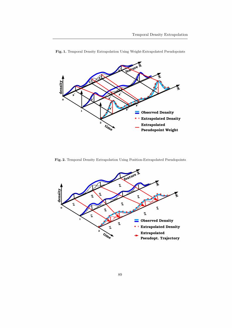
Temporal Density Extrapolation
Fig. 1. Temporal Density Extrapolation Using Weight-Extrapolated Pseudopoints
w2
w4
w3
w1
w2
w3
w1
w4
w2
w4
w3
w1
time
0
1
2
densit
y
feature X
X
X
Extrapolated Density
Observed Density
Extrapolated
Pseudopoint Weight
Fig. 2. Temporal Density Extrapolation Using Position-Extrapolated Pseudopoints
p2
p4
p3
p1
p4
p3
p1
p2
p4
p3
p1
p2
time
0
1
2
densit
y
feature X
X
X
Extrapolated Density
Observed Density
Extrapolated
Pseudopt. Trajectory
89

G. Krempl
as it influences the precision of the extrapolated values: in regions with sparsepseudo-point populations, the model is less flexible than in densely populatedones. Therefore, this approach seems better suited for constricted (bounded)feature spaces. A simple equidistant placement of pseudo-points distributes theprecision over the whole feature space. Alternatively, the pseudo-points might beplaced at the coordinates of a subsample of the observed instances, thus concen-trating the precision on areas with previously high density. However, if densitieschange largely over time, these areas might become less relevant.
In contrast, the second, position-extrapolating approach determines the po-sitions of each pseudo-point automatically. It aims to adjust the future locationof the pseudo-points such that they are densely placed in regions with a highexpected density. However, in the case polynomial regression functions are used,a potential drawback is that their trajectories diverge in the long run. Thus,in contrast to the first approach, the second one seems to be better suited forinfinite (unbounded) feature spaces.
Related to the choice of the pseudo-points’ placements is the question ofoptimal bandwidth selection, which for kernel density estimation has alreadybeen reviewed in [18]. In short, we expect that with an increasing number ofpseudo-points the optimal bandwidth decreases, while the extrapolation’s preci-sion increases. Furthermore, the number of pseudo-points is also an upper boundon the number of modes that both approaches are able to model.
4 Conclusion
In this paper, we have addressed the problem of temporal density extrapolation,where the objective is the prediction of a (potentially multi-modal) density dis-tribution at future time points, given a sample of historical instances observedat different positions in feature space and at different times in the past. Two ap-proaches based on pseudo-points were sketched: the first uses an extrapolation oftime-varying weights of stationary located pseudo-points, while the second usesan extrapolation of the trajectory of the time-varying location of pseudo-pointswith uniform weights. Subsequently, these extrapolated pseudo-points are usedin a kernel density estimation at future time points.
Having sketched the idea of the two temporal density extrapolation ap-proaches, a more detailed specification and evaluation of these methods needsto be done in future work. Furthermore, the conjectures in the discussion above,in particular the usability of each approach for bounded and unbounded fea-ture spaces, need to be verified. Finally, a known challenge for kernel-basedapproaches is the curse of dimensionality on multi-dimensional data. A naiveapproach is to combine multiple univariate temporal density extrapolations.However, an optimisation for multi-variate problems by using either projectionpursuit [4] or copula [12] techniques seems worth investigating.
90

Temporal Density Extrapolation
Acknowledgments. We thank Vera Hofer from Karl-Franzens-University Graz,Stephan Mohring, and Andy Koch for insightful discussions.
References
1. Aggarwal, C.C.: A framework for diagnosing changes in evolving data streams. In:Proceedings of the ACM SIGMOD Conference (2003)
2. Aggarwal, C.C.: On change diagnosis in evolving data streams. IEEE Transactionson Knowledge and Data Engineering 17(5), 587–600 (2005)
3. Bottcher, M., Hoppner, F., Spiliopoulou, M.: On exploiting the power of time indata mining. ACM SIGKDD Explorations Newsletter 10(2), 3–11 (2008)
4. Friedman, J.H., Stuetzle, W., Schroeder, A.: Projection pursuit density estimation.Journal of the American Statistical Association 79(387) (1984)
5. Hofer, V., Krempl, G.: Drift mining in data: A framework for addressing drift inclassification. Computational Statistics and Data Analysis 57(1), 377–391 (2013)
6. Hooker, G.: Diagnosing extrapolation: Tree-based density estimation. In: Knowl-edge Discovery in Databases (KDD) (2004)
7. Jeon, J., Taylor, J.W.: Using conditional kernel density estimation for wind powerdensity forecasting. Journal of the American Statistical Association 107 (2012)
8. Krempl, G.: The algorithm APT to classify in concurrence of latency and drift. In:Gama, J., Bradley, E., Hollmen, J. (eds.) Advances in Intelligent Data Analysis X,Lecture Notes in Computer Science, vol. 7014, pp. 222–233. Springer (2011)
9. Krempl, G., Hofer, V.: Classification in presence of drift and latency. In:Spiliopoulou, M., Wang, H., Cook, D., Pei, J., Wang, W., Zaıane, O., Wu, X.(eds.) Proceedings of the 11th IEEE International Conference on Data MiningWorkshops (ICDMW 2011). IEEE (2011)
10. Krempl, G., Zliobaite, I., Brzezinski, D., Hullermeier, E., Last, M., Lemaire, V.,Noack, T., Shaker, A., Sievi, S., Spiliopoulou, M., Stefanowski, J.: Open challengesfor data stream mining research. SIGKDD Explorations 16(1), 1–10 (2014), specialIssue on Big Data
11. Nadaraya, E.A.: Nonparametric estimation of probability densities and regressioncurves. Kluwer (1989), originally published in Russian by Tbilisi University Press,Translated by S. Klotz
12. Nelsen, R.B.: An Introduction to Copulas. Springer (1999)13. Parzen, E.: On estimation of a probability density function and mode. Annals of
Mathematical Statistics 33, 1065–1076 (1962)14. Rosenblatt, M.: Remarks on some non-parametric estimates of a density function.
Annals of Mathematical Statistics 27(3), 832–837 (1956)15. Skouras, K., Dawid, A.P.: On efficient probability forecasting systems. Biometrika
86(4), 765–784 (1999)16. Tay, A.S., Wallis, K.F.: Density forecasting: A survey. Companion to Economic
Forecasting pp. 45–68 (2002)17. Terrell, G.R.: Tail probabilities by density extrapolation. In: Proceedings of the
Annual Meeting of the American Statistical Association (2001)18. Turlach, B.A.: Bandwidth selection in kernel density estimation: A review. Tech.
Rep. 9307, Humboldt University, Statistic und Okonometrie (1991)
91

92

Proceedings 1st International Workshop on Advanced Analytics and Learning on Temporal DataAALTD 2015
Fuzzy Clustering of Series Using Quantile
Autocovariances
Borja Lafuente-Rego and Jose A. VilarResearch Group on Modeling, Optimization and Statistical Inference (MODES),Department of Mathematics, Computer Science Faculty, University of A Coruna
Abstract. Unlike conventional clustering, fuzzy cluster analysis allowsdata elements to belong to more than one cluster by assigning member-ship degrees of each data to clusters. This work proposes a fuzzy C–medoids algorithm to cluster time series based on comparing their esti-mated quantile autocovariance functions. The behaviour of the proposedalgorithm is studied on different simulated scenarios and its effectivenessis concluded by comparison with alternative approaches.
1 Introduction
In classical cluster analysis each datum is assigned to exactly one cluster, thusproducing a “hard” partition of the data set into several disjoint subsets. Thisapproach can be inadequate in the presence of data objects that are equally dis-tant to two ore more clusters. Fuzzy cluster analysis allows gradual membershipsof data objects to clusters, thus providing versatility to reflect the certainty withwhich each data is assigned to the different clusters. An interesting overview ofpresent fuzzy clustering methods is provided by [3]. Interest in this approachhas increased in recent years. Proof of this is the large amount of publicationsin this field (e.g. [6] and [5]).
In this paper, a fuzzy C–medoids algorithm to cluster time series using thequantile autocovariance functions is proposed. Motivation behind this approachis twofold. First, quantile autocovariances have shown a high capability to clus-ter time series generated from a broad range of dependence models [10]. On theother hand, the use of a fuzzy approach for clustering time series is justified inorder to gain adaptivity for constructing the centroids and to obtain a bettercharacterization of the temporal pattern of the series (see discussion in [7]). Toillustrate the merits of the proposed algorithm, an extensive simulation studycomparing our fuzzy approach with other fuzzy procedures has been carriedout. Specifically, we have focused on the classification of heteroskedastic models,which are of great importance in many applications (e.g. to model many finan-cial time series) and have received relatively little attention in the clusteringliterature.
2 A dissimilarity based on quantile autocovariances
Consider a set of p series S =XXX(1), . . . ,XXX(p)
, with XXX(j) = (X
(j)1 , . . . , X
(j)T )
being a T -length partial realization from a real valued process X(j)t , t ∈ Z.
Copyright c©2015 for this paper by its authors. Copying permitted for private and academicpurposes.
93

B. Lafuente-Rego, J.A. Vilar
We wish to perform cluster analysis on S in such a way that series with similargenerating processes are grouped together. To achieve this goal, we propose tomeasure dissimilarity between two series by comparing the estimators of theirquantile autocovariance functions (QAF), which are formally defined below.
Let X1, . . . , XT an observed stretch of a strictly stationary process Xt; t ∈Z. Denote by F the marginal distribution of Xt and by qτ = F−1(τ), τ ∈ [0, 1],the corresponding quantile function. Fixed l ∈ Z and an arbitrary couple ofquantile levels (τ, τ ′) ∈ [0, 1]2, consider the cross-covariance of the indicatorfunctions I (Xt ≤ qτ ) and I (Xt+l ≤ qτ ′) given by
γl(τ, τ′) = cov I (Xt ≤ qτ ) , I (Xt+l ≤ qτ ′) = P (Xt ≤ qτ , Xt+l ≤ qτ ′)− τ τ ′.
(1)Function γl(τ, τ
′), with (τ, τ ′) ∈ [0, 1]2, is called quantile autocovariance func-
tion of lag l. Replacing in (1) the theoretical quantiles of the marginal distribu-tion F , qτ and qτ ′ , by the corresponding empirical quantiles based onX1, . . . , XT ,qτ and qτ ′ , we obtain the estimated quantile autocovariance function given by
γl(τ, τ′) =
1
T − l
T−l∑
t=1
I (Xt ≤ qτ ) I (Xt+l ≤ qτ ′)− τ τ ′. (2)
As the quantile autocovariances are able to account for high level dynamic
features, a simple dissimilarity criterion between two series X(1)t and X
(2)t con-
sists in comparing their estimated quantile autocovariances on a common rangeof selected quantiles. Thus, for L prefixed lags, l1, . . . , lL, and r quantile levels,0 < τ1 < . . . < τr < 1, we construct the vectors ΓΓΓ (u), u = 1, 2, given by
ΓΓΓ (u) =(ΓΓΓ
(u)l1
, . . . ,ΓΓΓ(u)lL
), with ΓΓΓ
(u)li
=(γ(u)li
(τj , τk); j, k = 1 . . . , r), (3)
for i = 1, . . . , L, and γ given in (2). Then, the distance between X(1)t and X
(2)t
is defined as the squared Euclidean distance between their representations ΓΓΓ (1)
and ΓΓΓ (2), i.e.
dQAF
(X
(1)t , X
(2)t
)= ||ΓΓΓ (1) −ΓΓΓ (2)||22 (4)
Computing dQAF for all pairs of series in S allows us to set a pairwise dissim-ilarity matrix, which can be taken as starting point of a conventional hierarchicalclustering algorithm. Alternatively, a partitioning clustering, such as the k-meansalgorithm, can be performed averaging the ΓΓΓ representations to determine thecentroids. Then, dQAF is also used to calculate the distances between series andcentroids involved in the iterative refinement of the cluster solution.
3 Fuzzy clustering based on quantile autocovariances
Time series are dynamic objects and therefore different temporal patterns maybe necessary to characterize the serial behaviour in different periods of time. In
94

Fuzzy Clustering of Series Using Quantile Autocovariances
other words, the series are not distributed accurately within a given number ofclusters, but they can belong to two or even more clusters. This problem can beadequately treated using a fuzzy clustering procedure, which associates a fuzzylabel vector to each element stating its memberships to the set of clusters. Inthis section we propose a fuzzy C-medoids clustering algorithm for time seriesby plugging the QAF-dissimilarity introduced in Section 2.
Let S =XXX(1), . . . ,XXX(p)
be a set of p time series and ΓΓΓ =
ΓΓΓ (1), . . . ,ΓΓΓ (p)
a set of quantile autocovariances selected to perform clustering. The fuzzy C-
medoids clustering finds the subset of ΓΓΓ , ΓΓΓ =ΓΓΓ (1), . . . , ΓΓΓ (C)
, and the p ×
C matrix of fuzzy coefficients Ω = (ui,c) that lead to solve the minimizationproblem:
minΓ ,Ω
p∑
i=1
C∑
c=1
umic
∥∥∥ΓΓΓ (i) −ΓΓΓ (c)∥∥∥2
2, subject to
C∑
c=1
uic = 1 and uic ≥ 0. (5)
Each uic ∈ [0, 1] represents the membership degree of the i-th series to the c-thcluster and the parameter m > 1 controls the fuzziness of the partition. As thevalue ofm increases, the boundaries between clusters become softer and thereforethe classification is fuzzier. If m = 1, the hard version of the clustering procedureis obtained, i.e. uic ∈ 0, 1, that leads to a classical K-means partition of S.
The constraints∑C
c=1 uic = 1 and uic ≥ 0 ensure that no cluster is empty andthat all series are included in the cluster partition.
The objective function (5) cannot be minimized directly, and an iterativealgorithm that alternately optimizes the membership degrees and the medoidsmust be used. The update formula for the membership degrees is given by
uic =
C∑
c′=1
( ∥∥ΓΓΓ (i) −ΓΓΓ (c)∥∥22∥∥ΓΓΓ (i) −ΓΓΓ (c′)∥∥22
) 1
m−1
−1
, for i = 1, . . . , p. (6)
Then, the QAF-based fuzzy C–medoids clustering algorithm is implementedas follows.
i. Pick an initial set of medoids ΓΓΓ =ΓΓΓ (1), . . . , ΓΓΓ (C)
and the fuzzifier m.
ii. Set ΓΓΓOLD = ΓΓΓ .iii. Compute uic using (6).
iv. Update the medoids, let’s say ΓΓΓ =ΓΓΓ (1), . . . , ΓΓΓ (C)
, by minimizing the
objective function with the new uic. Denote by
q = argmin1≤i′<p
p∑
i′′=1
umi′′c
∥∥∥ΓΓΓ (i′′) −ΓΓΓ (i′)∥∥∥2
2
If the value of q is lower than the one obtained with ΓΓΓ , then ΓΓΓ = ΓΓΓ .v. If ΓΓΓOLD = ΓΓΓ or a maximum number of iterations is achieved then end
algorithm. Otherwise, return to step ii.
The total number of clusters C has to be preset. For this task classical indexessuch as silhouette width or Krazanowski-Lai index can be used.
95

B. Lafuente-Rego, J.A. Vilar
4 Simulation Study
The proposed fuzzy algorithm was tested against two other fuzzy clusteringalgorithms via simulation. In particular, the classification of heteroskedastictime series was considered by simulating two different scenarios formed by (i)GARCH(1,1) models and (ii) different structures of conditional heteroskedastic-ity. The selected generating models at each case are detailed below.
– Scenario 1: Consider Xt = µt + at, with µt ∼ AR(1) and at = σtǫt,ǫt ∼ N (0, 1). Then, the following GARCH(1,1) structures for the varyingconditional variance are considered:
M1: σ2t = 0.1 + 0.01a2t−1 + 0.9σ2
t−1 M3: σ2t = 0.1 + 0.1a2t−1 + 0.1σ2
t−1
M2: σ2t = 0.1 + 0.9a2t−1 + 0.01σ2
t−1 M4: σ2t = 0.1 + 0.4a2t−1 + 0.5σ2
t−1
– Scenario 2: Consider Xt = µt + at, with µt ∼ MA(1) and at = σtǫt,ǫt ∼ N (0, 1). Then, the following ARCH(1), GARCH(1,1), GJR-GARCHand EGARCH structures are considered for the varying conditional variance:
M1: σ2t = 0.1 + 0.8a2t−1
M2: σ2t = 0.1 + 0.1a2t−1 + 0.8σ2
t−1
M3: σ2t = 0.1 + (0.25 + 0.3Nt−1)a
2t−1 + 0.5σ2
t−1; Nt−1 = I(at−1 < 0)M4: ln(σ2
t ) = 0.1 + ǫt−1 + 0.3 [|ǫt−1| − E(|ǫt−1|)] + 0.4ln(σ2t−1)
In all cases ǫt consisted of independent zero-mean Gaussian variables withunit variance. For each scenario, five series of length T = 200 were generatedfrom each model over N = 100 trials.
Two fuzzy clustering algorithms specifically designed to deal with GARCHmodels were used and compared with our proposal. Both algorithms rely ondifferent dissimilarity measures constructed using the AR representation of aGARCH(p,q) process given by
σ2t = γ +
p∑
i=1
αia2t−i +
q∑
j=1
βjσ2t−j (7)
with γ > 0, 0 ≤ αi < 1 and 0 ≤ βj < 1, for i = 1, . . . , p and j = 1, . . . , q, and(∑p
i=1 αi +∑q
j=1 βj) < 1. Then, the dissimilarities are defined as follows.
1. Dissimilarity based on the autoregressive representation of the GARCHmod-els [12, 11]. Given XXX(k) and XXX(k′) in S, we define
d2AR(XXX(k),XXX(k′)) =
R∑
r=1
(πrk − πrk′)2,
with πrz an estimator of the r-th coefficient πr = (αr+βr)+∑min(q,r)
j=1 βjπr−j ,for the series z, z = k, k′. Parameter R determines the maximum number of
96

Fuzzy Clustering of Series Using Quantile Autocovariances
autoregressive coefficients πr. A GARCH–based fuzzy C-medoids clusteringis proposed in [4] by considering the optimization problem:
minΠ,Ω
p∑
i=1
C∑
c=1
umic
R∑
r=1
(πri − πrc)2, subject to
C∑
c=1
uic = 1 and uic ≥ 0. (8)
2. GARCH-based distance measure [1] given by
dGARCH(XXX(k),XXX(k′)) = (Lk −Lk′)
′(Vk + Vk′)
−1(Lk −Lk′) (9)
with Lj =
(αj, βj
)the vector of estimated parameters and Vj the esti-
mated covariance matrix for Lj , for j = k, k′. An alternative GARCH-basedfuzzy C-medoids clustering is proposed in [4] by minimizing:
p∑
i=1
C∑
c=1
umic
[(Li −Lc)
′(Vi + Vc)
−1(Li −Lc)
], (10)
subject to∑C
c=1 uic = 1 and uic ≥ 0.
The three fuzzy clustering algorithms were performed using a fuzziness pa-rameter m = 1.5 on N = 100 trials for each scenario. At each trial, the qualityof the clustering procedure was evaluated comparing the experimental clustersolution with the true cluster partition. Two different agreement measures wereused, namely the Gavrilov index [8] and the adjusted Rand index [9]. The meanvalues and standard deviations of these indexes based on the 100 trials usingboth hard and fuzzy cluster analysis are provided in Table 1.
Table 1. Averages and standard deviations (in brackets) of two cluster similarityindexes obtained from 100 trials.
Scenario 1 Scenario 2Gavrilov Adj. Rand Gavrilov Adj. Rand
Hard cluster dAR 0.859 (.109) 0.685 (.198) 0.712 (.146) 0.469 (.215)dGARCH 0.574 (.059) 0.286 (.072) 0.504 (.078) 0.137 (.116)dQAF 0.843 (.109) 0.726 (.152) 0.918 (.081) 0.825 (.135)
Fuzzy cluster dAR 0.541 (.056) 0.271 (.080) 0.486 (.076) 0.128 (.100)dGARCH 0.553 (.088) 0.241 (.132) 0.535 (.076) 0.188 (.107)dQAF 0.842 (.116) 0.704 (.181) 0.925 (.072) 0.833 (.125)
Results from Table 1 show that the metrics based on quantile autocovariancesand on the AR representation led to the best scores in Scenario 1 when the hardcluster is carried out. When the fuzzy approaches were considered, the behaviourof the dAR substantially worsened, while the very similar (even somewhat higher)
97
B. Lafuente-Rego, J.A. Vilar
results were obtained with dQAF . The worst results were obtained with theGARCH-based dissimilarity both for the hard and the fuzzy versions.
The metric based on quantile autocovariances also obtained the best resultsin Scenario 2, with indexes of agreement above 0.8 and a slight improvement byusing the fuzzy clustering. The GARCH-based metrics, dAR and dGARCH wherestrongly affected by the model misspecification and produced the worst resultsfor both the hard and the fuzzy versions of the cluster analysis.
To assess the effect of the fuzziness parameter in the partitions the algorithmwas implemented for several values of m. However this results were here omitteddue to the limitation of space.
5 A case study
In this section, the proposed fuzzy C–medoids clustering algorithm is used to per-form clustering on a set of series of electricity demand. Specifically, our databaseconsists of hourly electricity demand in the Spanish market from 1st January2011 to 31th December 2012. All data are sourced from the official website ofOperador del Mercado Iberico de Energia1. Records corresponding to Saturdaysand Sundays have been removed from the database because electricity demandis lower in the weekends. Thus we have 24 time series (one for each hour of theday) of length T = 731. Since all series are non–stationary in mean, the originalseries are transformed taking one regular difference.
Table 2 presents the membership degrees for the case with two and threeclusters. The results obtained for the two–cluster partition formed by C1 =H24, H1, H2, H3, H4, H5, H6, H7 and C2 grouping the remaining series. Thecluster C1 corresponds with the hours of the day where the electricity demandis low, while the C2 identifies the time of the day when the power consumptionis greater. In the case of the three–cluster partition, the cluster C1 is divided intwo subclusters. One formed with the hours of the day with the lowest demandof electricity, and a second cluster with an intermediate electricity consumption.
6 Concluding remarks
In this paper, we focus on the classification of time series featuring a fuzzyclustering algorithm in the framework of a partitioning around medoids. Adissimilarity–based approach is considered. In particular, we propose a C–medoidsfuzzy clustering algorithm using an innovative dissimilarity measure based on thequantile autocovariances (dQAF ).
The simulation study shows that the proposed dissimilarity produces satisfac-tory results by performing fuzzy cluster analysis. The proposed clustering algo-rithm was tested against two GARCH–based fuzzy clustering algorithm presentin the literature in two different heteroskedastic scenarios. The fuzzy clusteringalgorithm based on dQAF led to the best results. In fact, apart from dQAF , none
1 http://http://www.omel.es/files/flash/ResultadosMercado.swf
98

Fuzzy Clustering of Series Using Quantile Autocovariances
Table 2. Membership degrees obtained with QAF–based FCM with m = 1.5 consid-ering 2 and 3 clusters.
2 Clusters 3 Clusters
Membership degrees Crisp Membership degrees Crisp
C1 C2 C1 C2 C3
H1 0.63044 0.36956 1 1.00000 0.00000 0.00000 1H2 1.00000 0.00000 1 0.99878 0.00098 0.00024 1H3 0.98282 0.01718 1 0.99484 0.00395 0.00121 1H4 0.94118 0.05882 1 0.99229 0.00574 0.00197 1H5 1.00000 0.00000 1 0.92388 0.06811 0.00801 1H6 0.99923 0.00077 1 0.30793 0.66185 0.03021 2H7 0.98282 0.01718 1 0.00000 1.00000 0.00000 2H8 0.00003 0.99997 2 0.05793 0.09475 0.84733 3H9 0.00003 0.99997 2 0.00097 0.00294 0.99610 3H10 0.00077 0.99923 2 0.00045 0.00149 0.99806 3H11 0.00077 0.99923 2 0.00171 0.00507 0.99323 3H12 0.00002 0.99998 2 0.00011 0.00049 0.99940 3H13 0.00002 0.99998 2 0.00027 0.00178 0.99794 3H14 0.00002 0.99998 2 0.00032 0.00107 0.99861 3H15 0.00002 0.99998 2 0.00134 0.00940 0.98927 3H16 0.00002 0.99998 2 0.00088 0.00636 0.99277 3H17 0.00002 0.99998 2 0.00000 0.00000 1.00000 3H18 0.00056 0.99944 2 0.00051 0.00498 0.99451 3H19 0.00000 1.00000 2 0.00002 0.00014 0.99984 3H20 0.00003 0.99997 2 0.00020 0.00135 0.99846 3H21 0.00056 0.99944 2 0.00047 0.00384 0.99569 3H22 0.01718 0.98282 2 0.00136 0.01488 0.98377 3H23 0.00003 0.99997 2 0.01539 0.13091 0.85370 3H24 0.99998 0.00002 1 0.00206 0.98054 0.01740 2
of the remaining examined dissimilarities shown acceptable results by cluster-ing heteroskedastic processes, thus emphasizing the usefulness of dQAF in thisframework.
Note that a limitation of our procedure is that series are assumed to bestrictly stationary and hence further research must be carried out. Althoughwe have followed a dissimilarity-based approach, it is worthy to emphasize thatmodel-based techniques can be also an interesting alternative. Likewise the fuzzyapproach, the use of probabilistic models such as mixture models (see e.g. [2])allows us to assign each datum to one single cluster although this assignmentrelies on a probabilistic approach since the mixing proportions are estimatedfrom the data. Unlike the fuzzy approach, no fuzziness parameter is required byusing mixture models, although the model selection problem must be solved inthe latter case.
References
1. Caiado, J., Crato, N.: A garch-based method for clustering of financial time series:International stock markets evidence. Mpra paper, University Library of Munich,Germany (2007), http://EconPapers.repec.org/RePEc:pra:mprapa:2074
2. Chen, W.C., Maitra, R.: Model-based clustering of regression time series data viaapecman aecm algorithm sung to an even faster beat. Statistical Analysis and DataMining 4(6), 567–578 (2011)
99

B. Lafuente-Rego, J.A. Vilar
3. Doring, C., Lesot, M.J., Kruse, R.: Data analysis with fuzzy clustering methods.Computational Statistics & Data Analysis 51(1), 192 – 214 (2006)
4. D’Urso, P., Cappelli, C., Lallo, D.D., Massari, R.: Clustering of financial timeseries. Physica A 392(9), 2114–2129 (2013)
5. D’Urso, P., Giovanni, L.D., Massari, R.: Time series clustering by a robust autore-gressive metric with application to air pollution 141(15), 107–124 (2015)
6. D’Urso, P., Giovanni, L.D., Massari, R., Lallo, D.D.: Noise fuzzy clustering of timeseries by the autoregressive metric 71(3), 217–243 (2013)
7. D’Urso, P., Maharaj, E.A.: Autocorrelation-based fuzzy clustering of time series.Fuzzy Sets Syst. 160(24), 3565–3589 (2009)
8. Gavrilov, M., Anguelov, D., Indyk, P., Motwani, R.: Mining the stock market(extended abstract): Which measure is best? In: Proceedings of the sixth ACMSIGKDD International Conference on Knowledge Discovery and Data Mining. pp.487–496. KDD’00, ACM, New York, USA (2000)
9. Hubert, L., Arabie, P.: Comparing partitions. J. Classif. 2(1), 193–218 (1985)10. Lafuente-Rego, B., Vilar, J.A.: Clustering of time series using quantile autocovari-
ances. Advances in Data Analysis and Classification pp. 1–25 (2015)11. Maharaj, E.A.: Clusters of time series. J. Classification 17(2), 297–314 (2000)12. Piccolo, D.: A distance measure for classifying arima models. J. Time Series Anal.
11(2), 153–164 (1990)
100
Proceedings 1st International Workshop on Advanced Analytics and Learning on Temporal DataAALTD 2015
Causality on Longitudinal Data:
Stable Specification Search in Constrained
Structural Equation Modeling
Ridho Rahmadi1,2, Perry Groot2, Marianne Heins4,Hans Knoop3, and Tom Heskes2
1 Department of Informatics, Universitas Islam Indonesia.2 Institute for Computing and Information Sciences, Radboud University Nijmegen.3 Expert Centre for Chronic Fatigue, Radboud University Medical Centre, Nijmegen.
4 Netherlands Institute for Health Services Research, [email protected]
Abstract Developing causal models from observational longitudinal stud-ies is an important, ubiquitous problem in many disciplines. A disadvan-tage of current causal discover algorithms, however, is the inherent instabilityin structure estimation. With finite data samples small changes in thedata can lead to completely different optimal structures. The presentwork presents a new causal discovery algorithm for longitudinal datathat is robust for finite data samples. We validate our approach on asimulated data set and real-world data on Chronic Fatigue Syndromepatients.
Keywords: Longitudinal data, Causal modeling, Structural equationmodel, Stability selection, Multi-objective evolutionary algorithm.
1 Introduction
Developing causal models from observational longitudinal studies is an impor-tant, ubiquitous problem in many disciplines, which has led to the developmentof a variety of causal discovery algorithms in the literature [1–5]. A disadvantageof current causal discovery algorithms, however, is the inherent instability instructure learning. With finite data samples small changes in the data can leadto completely different optimal structures, since errors made by the discoveryalgorithm may be propagated and lead to further errors [6]. In [7] we developeda robust causal discovery algorithm for cross-sectional data. The method per-forms structure search over Structural Equation Models (SEMs) by maximizingmodel scores in terms of data fit and complexity. The present work extends ourcausal discovery algorithm to longitudinal data. We describe how longitudinalcausal relationships can be modelled for an arbitrary number of time slices. Fur-thermore, we show how a longitudinal causal model can easily be scored usingstandard SEM software by data reshaping. The algorithm produces accuratestructure estimates and is shown to be robust for finite samples. We validate ourapproach on one simulated longitudinal data set and one real-world longitudinaldata set for Chronic Fatigue Syndrome.
Copyright c©2015 for this paper by its authors. Copying permitted for private and academicpurposes.
101

R. Rahmadi, P. Groot, M. Heins, H. Knoop, T. Heskes
2 Proposed method
We use a SEM for causal modeling. The general form of the equations is
xi = fi(pai, εi), i = 1, . . . , n. (1)
where pai denotes the parents which represent the set of variables considered tobe direct causes of Xi and εi represents errors on account of omitted factors thatare assumed to be mutually independent [8]. In this study, we focus on causalmodels with no reciprocal relationships, and no latent variables. Thus the causalmodel can also be represented by a Directed Acyclic Graph (DAG). We scoremodels using both the chi-square χ2 (measuring the data fit) and the model
complexity (measuring the number of parameters).We use the method we developed in [7] to perform exploratory search over
SEM models. Based on the idea of stability selection [9], the method subsamplesthe data D with size ⌊|D|/2⌋ without replacement and generates Pareto optimalmodels for each subset. After that, all Pareto optimal models are transformedinto their corresponding model equivalent classes, called Completed Partially Di-
rected Acyclic Graph (CPDAG) [10]. From these CPDAGs we compute the edgeand causal path stability graph, such as Figure 3a, by grouping them accordingto model complexity and computing their selection probability, i.e., the numberof occurrences divided by the total number of models for a certain level of modelcomplexity. Stability selection is then performed by specifying two thresholds,πsel (boundary of selection probability) and πbic (boundary of complexity). Forexample, setting πsel = 0.6 means that all causal relationships with edge sta-bility or causal path stability (Figure 3) above this threshold are consideredstable. The second threshold πbic is used to control overfitting. We set πbic tothe level of model complexity at which the minimum average Bayesian Infor-
mation Criterion (BIC) score is found. For example, πbic = 7 means that allcausal relationships with an edge stability or a causal path stability lower thanthis threshold (Figure 3) are considered parsimonious. Causal relationships thatintersect with the top-left region are considered both stable and parsimoniousand called relevant, from which we can derive a causal model.
The method in [7] only handles cross-sectional data. Based on the idea of“unrolling” the network in Dynamic Bayesian Networks [4, 5], we extended themethod to handle longitudinal data. We model longitudinal causal relationshipswith a SEM model consisting of two time slices (Figure 1a) that can be “un-rolled” into a network with an arbitrary number of time slices (Figure 1b). Timeslice ti represents the relationships within a time slice (intra-slice causal relation-ships, solid arcs in Figure 1a). Causal relationships between time slices (inter-slicecausal relationships, dashed arcs in Figure 1a) always go forward in time, i.e.,from time slice ti−1 to time slice ti.
To score our models on longitudinal data we use data reshaping. In thereshaped data, the first n data points contain the relations that occur in thefirst two time slices t0 and t1. The next n data points contain the relationsthat occur in time slices t1 and t2. The i-th subset of n data points contain
102

Causality on Longitudinal Data
ଵ
ଶ
ଷ
ସ
ଵ
ଶ
ଷ
ସ ݐଵ ݐ (a)
ଵ
ଶ
ଷ
ସ
ଵ
ଶ
ଷ
ସ
ଵ
ଶ
ଷ
ସ ݐ ݐଵ ݐଶ
(b)
Figure 1: (a) The longitudinal causal model. (b) The “unrolled” causal graphused to generate longitudinal data. It contains four continuous variables(X1, . . . , X4) in three different time slices t0, . . . , t2.
the relations in time slices ti−1 and ti. The reshaped data then allows us to usestandard SEM software to compute the scores.
3 Application to Simulated Data
For this experiment, we generated a longitudinal data set with 400 instancesfrom a causal graph as depicted in Figure 1b. The data set consists of three timeslices with four continuous variables for each time slice.1 When we searched overSEM models we added prior knowledge that variables X1 and X2 do not causevariable X3 directly. We performed the search over 200 subsets.
As the true model is known, we measure the performance of our method bymeans of the Receiver Operating Characteristic (ROC) [11] for both edges andcausal paths. The threshold πsel is fixed to a value (πsel ∈ 0.3, 0.6, 0.8, 0.9)while πbic is varied. We compute the True Positive Rate (TPR) and the False
Positive Rate (FPR) from the CPDAG of the true model. As for an example,in the case of edge stability, a true positive means that an edge that appearswithin the top-left region bounded by πsel and πbic also exists in the CPDAG ofthe true model. Figure 2 portrays the ROC curves for both edge and causal pathstability. Generally we can see that higher values of πsel tend to give better ROCcurves. This suggests that our approach is able to find the underlying structurewith high reliability scores. A notable point is that the ROC curves stop at aTPR and/or FPR value lower than 1. Since some of the edges and paths aredisallowed (i.e., no edges in time-slice ti−1 and no paths from ti to ti−1) someof the edges and causal paths in the stability graphs end up with a selectionprobability of 0 and the result is that the ROC curves cannot reach the upperright corner with TPR = FPR = 1.
1Available at http://bit.ly/1L6dBOo
103

R. Rahmadi, P. Groot, M. Heins, H. Knoop, T. Heskes
0.0 0.1 0.2 0.3 0.4 0.5 0.6 0.7
0.0
0.2
0.4
0.6
0.8
1.0
FPR
TPR
0.30.60.80.9
(a)
0.00 0.05 0.10 0.15 0.20 0.25 0.30
0.0
0.2
0.4
0.6
0.8
1.0
FPR
TPR
0.30.60.80.9
(b)
Figure 2: A plot of ROC curves for (a) the edge stability and (b) the causal pathstability, for different values of πsel. A higher πsel shows a better ROC curve. Seethe main text for an explanation why the ROC curves stop at some point.
4 Application to Real-world Data
For an application to real-world data, we consider a data set about Chronic
Fatigue Syndrome (CFS) which consists of 183 subjects and five time sliceswith six discrete variables [12]. The variables are, fatigue severity, the senseof control over fatigue, focusing on the symptoms, the objective activity of thepatient (oActivity), the subject’s perceived activity (pActivity), and the physicalfunctioning. We use Expectation Maximization implemented in SPSS [13] toimpute the missing values. As all of the variables have large scales, e.g., in therange between 0 to 155, we treat them as continuous variables. We added priorknowledge that the variable fatigue does not cause any of the other variablesdirectly. We performed the search over 200 subsets.
Figure 3a shows that nineteen relevant edges were found, consisting of elevenintra-slice and eight inter-slice relationships which among of these, six are betweenthe same variables and two are between different variables. Figure 3b shows thatthirty-two relevant causal paths were found, consisting of twelve intra-slice andtwenty inter-slice relationships which among of these, six are between the samevariables and fourteen are between different variables. For a more intuitive rep-resentation, we combine the stability graphs into a model using the followingprocedure. First, the nodes are linked according to the nineteen relevant edges.Second, edges are oriented according to our background knowledge. Eight of theinter-slice relationships are oriented from time slice ti−1 to ti and five of theintra-slice edges can be oriented since it is known that the variable fatigue doesnot directly cause any other variable. Third, the edges are oriented according tothe relevant causal paths, which results in another twenty-eight directed edges.The inferred model is shown in Figure 4. Each edge is annotated with a reliabil-ity score which is the maximum score obtained in the top-left region of the edgestability graph.
104

Causality on Longitudinal Data
Model complexity
Sel
ectio
n pr
obab
ility
0 2 4 6 8 11 14 17 20 23 26 29 32 35 38 41 44 47 50
00.
20.
40.
60.
81
pbic
psel
(a)
Model complexity
Sel
ectio
n pr
obab
ility
0 2 4 6 8 11 14 17 20 23 26 29 32 35 38 41 44 47 50
00.
20.
40.
60.
81
pbic
psel
(b)
Figure 3: The stability graphs for CFS together with πsel and πbic, yielding fourregions. The top-left region contains the relevant causal relations. (a) The edgestability graph. (b) The causal path stability graph. Orange-dashed lines rep-resent inter-slice relationships between the same variables, black-dotted linesrepresent inter-slice relationships between different variables, green-solid linesrepresent intra-slice relationships.
From the stability graphs we can see that the most stable causal relations arethe inter-slice relations between the same variables followed by some of the intra-slice causal relations. Almost all of the inter-slice relations between different vari-ables are not considered relevant. A directed edge X → Y in Figure 4 indicates
105

R. Rahmadi, P. Groot, M. Heins, H. Knoop, T. Heskes
that a change in variableX causes a change in variable Y . In the intra-slice causalrelationships, we found that all variables are direct causes for fatigue severity.We also found all variables, except fatigue, to be direct causes for the perceivedactivity. Furthermore, the variable control is a direct cause for both focusingon the symptoms and physical functioning. Generally the inter-slice relation-ships show direct causes between the same variables. In addition, the variablespActivity and control indicate a stronger direct cause for fatigue severity andfocusing on symptoms, respectively, as they contribute a direct cause in bothtime slices. The inferred model is consistent with results reported in the medicalliterature [12, 14,15].
control(ݐ୧ଵ)
pActivity(ݐ୧ଵ)
oActivity(ݐ୧ଵ)
functioning(ݐ୧ଵ)
focusing(ݐ୧ଵ)
fatigue(ݐ୧ଵ)
control(ݐ୧)
pActivity(ݐ୧) oActivity(ݐ୧)
functioning(ݐ୧) focusing(ݐ୧)
fatigue(ݐ୧) 1
0.93
1
1
1
1
1
0.64
1
0.71
1
0.96
1
1
0.61
0.91
0.99
0.99 1
Figure 4: The inferred model of CFS by combining the edge stability and causalpath stability graphs.
5 Conclusion
Causal discovery from longitudinal data is an important, ubiquitous problemin science. Current causal discovery algorithms, however, have difficulty dealingwith the inherent instability in structure estimation. The present work intro-duces a new discovery algorithm for longitudinal data that is robust for finitesamples. Experimental results on both artificial and real-world data sets showthat the method results in reliable structure estimates. Future research will aimto estimate the size of causal effects.
Acknowledgments
The research leading to these results has received funding from the DGHEof Indonesia and the European Community’s Seventh Framework Programme(FP7/2007-2013) under grant agreement n 305697.
106

Causality on Longitudinal Data
References
1. Riva, A., Bellazzi, R.: Learning temporal probabilistic causal models from longi-tudinal data. Artificial Intelligence in Medicine 8(3) (1996) 217–234
2. Parner, J., Arjas, E.: Causal reasoning from longitudinal data. Rolf NevanlinnaInst., University of Helsinki (1999)
3. Marsh, H.W., Yeung, A.S.: Causal effects of academic self-concept on academicachievement: Structural equation models of longitudinal data. Journal of educa-tional psychology 89(1) (1997) 41–54
4. Friedman, N., Murphy, K., Russell, S.: Learning the structure of dynamic proba-bilistic networks. In: Proceedings of the Fourteenth conference on Uncertainty inartificial intelligence, Morgan Kaufmann Publishers Inc. (1998) 139–147
5. Murphy, K., Mian, S., et al.: Modelling gene expression data using dynamicBayesian networks. Technical report, Computer Science Division, University ofCalifornia, Berkeley, CA (1999)
6. Spirtes, P.: Introduction to causal inference. The Journal of Machine LearningResearch 11 (2010) 1643–1662
7. Rahmadi, R., Groot, P., Heins, M., Knoop, H., Heskes, T., The OPTIMISTICconsortium: Causality on cross-sectional data: Stable specification search in con-strained structural equation modeling. arXiv:1506.05600 [stat.ML] (2015)
8. Pearl, J.: Causality: models, reasoning and inference. Cambridge Univ Press (2000)9. Meinshausen, N., Buhlmann, P.: Stability selection. Journal of the Royal Statistical
Society: Series B (Statistical Methodology) 72(4) (2010) 417–47310. Chickering, D.M.: Learning equivalence classes of Bayesian-network structures.
The Journal of Machine Learning Research 2 (2002) 445–49811. Fawcett, T.: ROC graphs: Notes and practical considerations for researchers. Ma-
chine learning 31 (2004) 1–3812. Heins, M.J., Knoop, H., Burk, W.J., Bleijenberg, G.: The process of cognitive
behaviour therapy for chronic fatigue syndrome: Which changes in perpetuatingcognitions and behaviour are related to a reduction in fatigue? Journal of psycho-somatic research 75(3) (2013) 235–241
13. IBM Corp. Armonk, NY: IBM SPSS Statistics for Windows, Version 19.0. (2010)14. Vercoulen, J., Swanink, C., Galama, J., Fennis, J., Jongen, P., Hommes, O., Van der
Meer, J., Bleijenberg, G.: The persistence of fatigue in chronic fatigue syndromeand multiple sclerosis: development of a model. Journal of psychosomatic research45(6) (1998) 507–517
15. Wiborg, J.F., Knoop, H., Frank, L.E., Bleijenberg, G.: Towards an evidence-basedtreatment model for cognitive behavioral interventions focusing on chronic fatiguesyndrome. Journal of psychosomatic research 72(5) (2012) 399–404
107

108

Proceedings 1st International Workshop on Advanced Analytics and Learning on Temporal DataAALTD 2015
CourboSpark: Decision Tree
for Time-series on Spark
Christophe Salperwyck1, Simon Maby2, Jerome Cubille1, and MatthieuLagacherie21 EDF R&D,
1 avenue du General de Gaulle, 92140 Clamart, France2 OCTO Technology,
50 avenue des Champs-Elysees, 75008 Paris, France
Abstract. With the deployment of smart meters across many countries,data are being collected at a large scale and volume. These data arecollected for billing purposes but also to get analytical insights. Ourmain goal here is to build an understandable model able to explain theelectric consumption patterns regarding several features. We chose to usedecision tree models as they are easily comprehensible and have alreadybeen parallelized with success. In our industrial context, we often haveto work on electrical time-series where the target to predict is neither alabel (classification) nor a numerical value (regression) but a time-seriesrepresenting a load curve. Therefore we use a different split criterionto separate time-series: the inertia. We also need a dedicated methodfor categorical features since the standard implementation would notwork for time-series. This method is based on a hierarchical clusteringin order to have a good trade-off between the computational complexityand the exploration of the possible bi-partition splits. We demonstratethe performance of our implementation on datasets with different sizes(up to a terabyte).
Keywords: CourboTree, Hadoop, Spark, Decision Tree, Parallelization
1 Introduction
With the deployment of smart meters across many countries, data are beingcollected at a large scale and volume. Electric meters measure and transmitelectric power consumption from every individual household and enterprise at arate of a measurement from every 24 hours down to 10 minutes to a centralizedinformation system. In France, EDF provides electricity to more than 35 mil-lion customers leading to a massive amount of data to process. These data arecollected for billing purposes but also to get analytical insights. Our main goalin this paper is to build an understandable model able to explain the electricalconsumption patterns regarding several features such as localization or type ofcontract. We chose to use decision tree models as they are easily comprehensibleand have already been parallelized with success in the Hadoop ecosystem.
CourboSpark is part of the X-Data project: http://www.xdata.fr/
Copyright c©2015 for this paper by its authors. Copying permitted for private and academicpurposes.
109

C. Salperwyck, S. Maby, J. Cubille, M. Lagacherie
Decision trees are well known methods in machine learning which are mainlyused for classification and regression tasks. In our industrial context, we oftenhave to work on electrical time-series where the target to predict is neither a label(classification) nor a numerical value (regression) but a time-series representinga load curve. Many versions of decision trees were proposed on top of Hadoop.The Spark [3] implementation seems to be the most suitable for our use-case.Therefore we extended the current Spark/MLlib [4] implementation of decisiontrees so that it can deal with a time-series as a target.
We first present previous work on parallel decision trees and explain whywe choose to reuse the MLlib implementation. Then we describe the time-seriesregression problem. In section 4, the inertia criterion used to separate time-seriesis presented. Section 5 will focus on the algorithm adaptation for categorical fea-tures with a method based on a hierarchical clustering. Finally, we demonstratethe performance of our implementation on datasets with different sizes (up to aterabyte).
2 Previous work on parallel decision trees
Our goal is to port our in-house software, CourboTree [1, 2], into a distributedsystem so that more data can be processed. Our CourboTree software builddecision tree on time-series based on the inertia criterion.
Many implementations of parallel decision trees have been proposed. In thispaper we focus on implementations that can run on top of Hadoop. Hadoopclusters offer a very good trade-off between computing power/storage and price.Hadoop is based on horizontal scaling: the computing power/storage is quasilin-ear with the number of nodes in the cluster. To have more power, more nodeshave to be added into the cluster. Table 1 presents different implementationsof decision trees on Hadoop. We used the following criteria to compare theseimplementations:
– partitioning: horizontal means the algorithm will parallelize computationson the lines, vertical on the columns of the dataset;
– engine: the execution engine that will run the parallel algorithm. These en-gines can also optimize the execution graph of the algorithm (as for Spark);
– target type: categorical for classification, numerical for regression (can beboth)
– ensemble: ability to build an ensemble of trees (random forest, bagging ofrandom trees...)
– pruning: does the algorithm prune the tree to avoid over-fitting?– open-source: is the source code available so that we can easily reuse it?
As we aimed to reuse an open-source implementation and our datasets mainlygrow in an horizontal way, we choose to adapt the MLlib implementation. More-over it uses the Spark engine which is faster than the original Map/Reduce enginein Hadoop.
110

CourboSpark
Partitionning Engine Target type Ensemble Pruning Open-source
MLlib [4] Horizontal Spark Num + Nom Yes No Yes
MR C4.5 [5] Vertical MR Nom No No No
PLANET [6] Horizontal MR Num + Nom Yes No No
SAMOA [7] Vertical Storm/S4 Num + Nom Yes Yes Yes
Table 1. Comparison of parallel decision trees in the Hadoop ecosystem (MR: originalMap-Reduce, Storm/S4: streaming frameworks, Spark: new computing engine – widelyused to replace MR).
3 Problem description: time-series regression
The problem is the same as the one stated in CourboTree [1, 2]: explain loadcurves pattern using explanatory features. It can be seen as time-series regres-sion. For this problem, we define our dataset as follows:
– 1, ..., n: the examples of the dataset;– w1, ..., wn: the weights of the examples;– X1, ..., Xj , ..., Xp: the p explanatory features where xij is the value for the
example i for Xj , these features can be either numerical or categorical;– Y1, ..., Yk, ..., Yq: the q numerical variables defining the time-series where yik
is the value for the example i for Yk. This time-series is the target of theregression.
Therefore an example i is described as the following tuple: wi, xi1...xip, yi1...yiq.There can be missing values for either the explanatory features or the time-series.
As in CourboTree, the model used to explain the load curves is a tree:
– l: a node/leaf of the tree,– gl: the center of gravity of the examples in l. Its coordinates gl1, . . . , glq are
the weighted mean of the examples in the node/leaf l for the q points of thetime-series Y .
4 Split criteria: inertia
Decision trees used in classification aim to lower the impurity in the leaves anduse a criterion such as the entropy gain or the Gini coefficient. For regressiontask, variance reduction is often used. As we deal with time-series we want tolower the variance between the time-series within a leaf/node. In this paper weuse the euclidean distance to compute the variance. Other distances could beused.
Given a node t, its intra inertia is defined as:
Iw(l) =∑
i∈l
wi
∑
k=1,...,q
(yik − glk)2
111

C. Salperwyck, S. Maby, J. Cubille, M. Lagacherie
This criteria can be used in the same way as the criterion used in classificationand regression trees. The best split to divide a leaf l into two leaves lL and lR isthe one minimizing the intra-inertia of these two new leaves:
argmin
(
Iw(lL) + Iw(lR)
)
Computing this intra-inertia is expensive but we can use the Konig-Huyghenstheorem which states that the global inertia is the sum of the intra-inertia Iwand inter-inertia IB :
I = Iw + IB
Therefore we can maximize the inter-inertia instead of minimizing the intra-inertia (which is also known as the “Ward’s method” [8] in statistics). Thiscorresponds to find the centers of gravity of the two new leaves which are thefurthest possible (relatively to their center weights). The computation of theinter-inertia is much more effective. For each potential split points we do notneed to recompute the intra-inertia on all the points to the two new centers ofgravity, but just the distance between the two new centers of gravity.
For times-series this means to maximize the distance between the averagecurves in the two leaves (lL, lR) having weights (wL, wR):
argmax
(
wL.wR
wL + wR
∑
i∈1...q
(gLi − gRi)2
)
As computing the inter-inertia criterion is more effective we have only usedthis criterion in CourboSpark. Both criteria are sums that can be parallelized.Therefore the computation can be easily spread across the nodes in the clusterin order to take advantage of its computational power.
5 Categorical variables: hierarchical clustering
For numerical feature, the MLlib algorithm has a parameter to specify the num-ber of “bins” that will be tested as split points. These bins correspond to quan-tiles computed on a random sample of the whole dataset. For the categoricalfeatures the next section explains how the current implementation works andhow it was adapted for time-series.
Building a binary decision tree with categorical feature requires to evaluateall the bi-partition/split of the modalities. The bi-partition with the lowest valueof the criteria is the one chosen to split the node into two leaves. This evaluationcan be costly as for m modalities there are (2m−1
− 1) possible bi-partitions.With m up to 30, the computation of all these partitions can be computed ina reasonable time (less than a minute on recent hardware). Our datasets havecategorical features up to 100 modalities (the number of French departmentsfor example). An exhaustive test of all the bi-partitions would take too muchtime as the number of bi-partitions to test is exponential with the number ofmodalities.
112
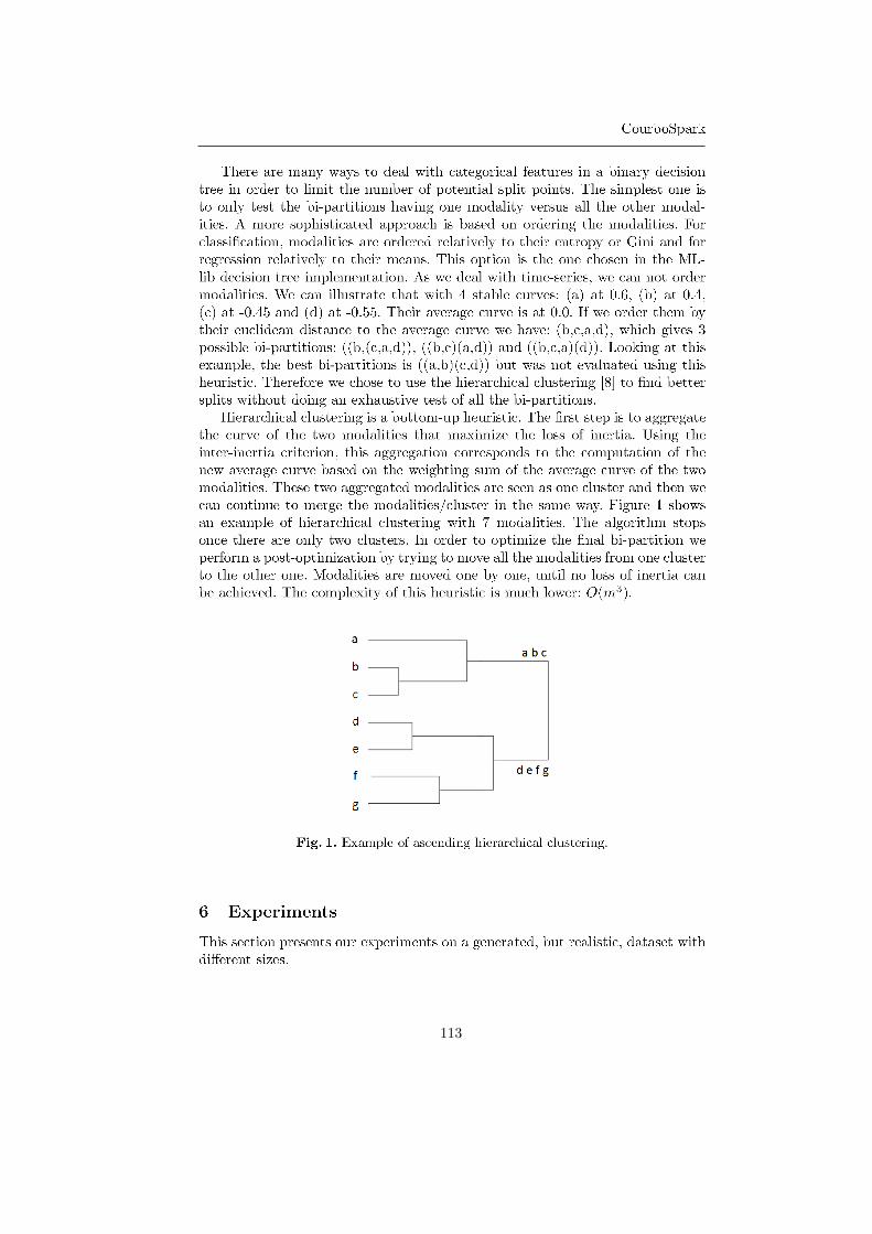
113

C. Salperwyck, S. Maby, J. Cubille, M. Lagacherie
Dataset: In order to control the experiments we have developed a generator.This generator takes as parameters: the depth of the tree, number of points inthe time-series, number of features, number of modalities for categorical features.We configured the generator to have a tree of depth 4, with 10 numerical and 10categorical features (50 modalities each). Each time-series has 144 points (stepof 10 minutes for one day). We generated from 10 to 1,000 millions time-series.
Configuration: The experiments were run on a cluster of 10 machines. Eachmachine has 32 cores, 48 GB of RAM and 14 SATA spinning disks. Spark wasconfigured to run with 9 executors with 20 GB and 8 cores each.
Results: The results of the the experimentation are presented in Figure 2. As wecan see the Spark MLlib implementation of decision tree scales almost linearlywith the dataset size.
0
50
100
150
200
250
300
350
400
0 200 400 600 800 1000 1200 1400
Tim
e i
n m
inu
tes
Data in GB
Fig. 2. Time to build the tree depending on the dataset size (10 to 1,000 millionscurves).
More experiments were conducted with similar results. We tested datasetswith up to 100 features, and also up to 500 modalities for categorical features.
7 Future works
We plan to extend our implementation so that it can deal with “cyclic features”as day of the week, month of the year... which are common in our datasets.
114

CourboSpark
This case is similar to numerical feature but gives two times more possible splitpoints.
The MLlib library only build trees which are balanced (each leaf is at thesame depth). The current CourboTree implementation first grows the part of thetree that gives the greatest loss of inertia and therefore can produce unbalancedtrees. As we would like to have the lowest global inertia for a given number ofleaves, we would either need to drive the tree construction to expand just a partof the tree or to do post-pruning to remove parts of the tree. A next step couldbe to use this pruning to control over-fitting.
More generally we plan to do more extensive tests to study how the Sparkconfiguration (number of executors, memory...) impact performance dependingon the datasets properties (number of features, modalities/bins...).
References
1. Stephan, V., Cogordan, F.: Courbotree : Application Des Arbres De RegressionMultivaries Pour La Classification De Courbes. XXXVIemes Journees de statistiquea Montpellier. http://www.agro-montpellier.fr/sfds/CD/textes/stephan1.pdf
2. Stephan, V.: CourboTree : Une Methode de Classification de Courbes Appliquee auLoad Profiling pp. 129–138. Revue MODULAB 33 (2005). http://www.modulad.fr/archives/numero-33/stephan-33/stephan-33.pdf
3. Zaharia M., Chowdhury M., Franklin M.J., Shenker S., Stoica I.: Spark: ClusterComputing with Working Sets, Proceedings of the 2nd USENIX conference on Hottopics in cloud computing (2010).
4. Amde M., Das H., Sparks E. Talwalkar A.: Scalable Distributed DecisionTrees in Spark MLLib, Spark Summit 2014. http://spark-summit.org/wp-
content/uploads/2014/07/Scalable-Distributed-Decision-Trees-in-Spark-
Made-Das-Sparks-Talwalkar.pdf
5. Dai W., Wei J.: A MapReduce Implementation of C4.5 Decision Tree Algorithm.International Journal of Database Theory and Application. Vol. 7, No. 1, pp. 49–60(2014) http://www.chinacloud.cn/upload/2014-03/14031920373451.pdf
6. Panda B., Herbach J., Basu S., Bayardo R.: PLANET: massively parallel learning oftree ensembles with MapReduce. Proceedings of the VLDB Endowment, pp. 1426–143 (2009).
7. De Francisci Morales G. , Bifet A.: SAMOA: Scalable Advanced Massive OnlineAnalysis. Journal of Machine Learning Research, Volume 16, pp. 149–153 (2015).
8. Ward, J. H. : Hierarchical Grouping to Optimize an Objective Function. Journal ofthe American Statistical Association 58 , no. 301 pp. 236–244 (1963).
115

116

Proceedings 1st International Workshop on Advanced Analytics and Learning on Temporal DataAALTD 2015
Anomaly Detection in Temporal Graph Data:
An Iterative Tensor Decomposition and Masking
Approach
Anna Sapienza1,2, Andre Panisson2, Joseph Wu3,Laetitia Gauvin2,∗, Ciro Cattuto2
1 Polytechnic University of Turin, Turin, Italy2 Data Science Laboratory, ISI Foundation, Turin, Italy
3 School of Public Health, University of Hong Kong, Hong Kong
Abstract. Sensors and Internet-of-Things scenarios promise a wealthof interaction data that can be naturally represented by means of time-varying graphs. This brings forth new challenges for the identification andremoval of temporal graph anomalies that entail complex correlations oftopological features and activity patterns. Here we present an anomalydetection approach for temporal graph data based on an iterative tensordecomposition and masking procedure. We test this approach using high-resolution social network data from wearable sensors and show that itsuccessfully detects anomalies due to sensor wearing time protocols.
Keywords: Data cleaning, anomaly detection, non-negative tensor fac-torization, high-resolution social networks, sensors, temporal networks.
1 Introduction
Emerging applications in the big data and Internet-of-Things domains pose newproblems for data cleaning. Time-resolved interaction data, in particular, areespecially challenging because the relational nature of the data yields anomaliesthat entangle temporal and topological aspects. Several studies have focused onidentifying anomalous behaviors in graph-based datasets [1] and time-varyingnetworks [2]. However, mesoscale anomalies that mimic normal behaviors areobserved in empirical data and call for further research.
Here we focus on time-varying graphs [3] represented as three-mode tensorsand we present an semi-supervised anomaly detection method based iterativetensor decomposition and masking. We report on the performance of this methodin detecting and removing anomalies in an empirical social network dataset gath-ered by using wearable proximity sensors in a school.
2 Methodology
A static graph can be represented by an adjacency matrix M ∈ RN×N , where
Mij = 1 if a contact between i and j occurred and Mij = 0 otherwise. Thisdescription can be generalized to the case of a time-varying graph, by using asequence of S consecutive adjacency matrices, that can be easily arranged as atensor T ∈ R
N×N×S .
Copyright c©2015 for this paper by its authors. Copying permitted for private and academicpurposes.
117

A. Sapienza, A. Panisson, J. Wu, L. Gauvin, C. Cattuto
The extraction of latent structures can then be performed by following theiterative approach described below. This framework allows to carry out the datacleaning by unearthing at each iteration group behaviours of nodes having cor-related activities and classifying these patterns of activities as meaningul oranomalous.
Step 1. The Non-negative Tensor Factorization [6] is used as a powerful toolto approximate the tensor T as a sum of R rank-one tensors ar br cr, calledcomponents. In the specific case of temporal networks, ar and br provide themembership of nodes to the component r, whereas cr is the temporal activitypattern of the component. Moreover, it is possible to consider ar ≈ br if thegraph is undirected. The components can be recovered by solving an optimizationproblem with non-negative constraints. The minimization problem
min
∥
∥
∥
∥
∥
tijk −
R∑
m=1
R∑
n=1
R∑
l=1
aimajnckl
∥
∥
∥
∥
∥
2
F
s.t. aim, ajn, ckl ≥ 0 (1)
is computed by the alternating non-negative least squares method [7], solvedby using the block principal pivoting algorithm [8]. The selection of a suitablenumber R of components is guided at each iteration by the Core ConsistencyDiagnostic [9, 10], and performed in order to prevent overfitting.
Step 2. The extracted components are analysed in order to discriminatebetween those dominated by anomalous activities or meaningful behaviours. Tothis end, a classifier working on the temporal activity patterns of each componentcr was developed.
Step 3. Spurious contact patterns highlighted by the anomalous componentsare combined into a mask, used to clean the original tensor. The nodes involvedin each of these contacts are detected by analysing the level of membershipgiven by ar. The occurrence times of these contacts are given by the anomalouswindows found in the temporal patterns cr. These windows are recovered byusing a step detection algorithm based on the Otsu threshold [11].
Step 4. The mask is applied to the tensor T in order to erase the invalidentries. The cleaned tensor T ′ becomes then the input of the consecutive iterationin the iterative framework.
Step 5. The procedure is repeated until no component is classified as anoma-lous in step 2.
3 Results and Validation
The current investigation involves the analysis of a high-resolution dataset whichdescribes the interactions of people in a primary school in Hong Kong. The schoolpopulation consisted in 709 children and 65 teachers divided into 30 classes. Datawere collected by using wearable proximity sensors [4, 5] over 10 consecutive daysin March 2013, from Monday 18th to Thursday 27th. These sensors record spatialproximity with a resolution of 20s. As a result, a time-varying network withN = 774 nodes was created. The data were then aggregated over a time-windowof 5min, leading to a division of the overall network in S = 2680 snapshots.
118

119

120

Anomaly Detection in Temporal Graph Data
References
1. W. Eberle, L. Holder, Discovering structural anomalies in graph-based data.In ICDM Workshops, pp. 393-398, 2007.
2. M. Mongiovi, et al., Netspot: Spotting significant anomalous regions on dy-namic networks. SIAM International Conference on Data Mining, 2013.
3. P. Holme, J. Saramaki. Temporal networks. Phys. Reps. 519:97-125, 2012.4. J. Stehle, N. Voirin, A. Barrat,C. Cattuto, L. Isella, et al. High-resolution
measurements of face-to-face contact patterns in a primary school. PLoS One
6:e23176, 2011.5. C. Cattuto, et al. Dynamics of person-to-person interactions from distributed
RFID sensor networks. PLoS ONE 5:e11596, 2010.6. T.G. Kolda and B.W. Bader. Tensor decompositions and applications. SIAM
Review, 51(3):455-500, 2009.7. H. Kim, L. Elde n, and H. Park. Non-negative tensor factorization based on
alternating large-scale nonnegativity-constrained least squares. In Proceedings
of IEEE 7th International Conference on Bioinformatics and Bioengineering
(BIBE07), volume II, pages 1147-1151, 2007.8. J. Kim and H. Park. Fast nonnegative tensor factorization with an active-
set-like method. In High-Performance Scientific Computing, Springer, London,2012, pp. 311-326
9. R. Bro and H. A. L. Kiers, A new efficient method for determining the numberof components in PARAFAC models, Journal of Chemometrics, 17 (2003), pp.274-286.
10. E.E. Papalexakis and C. Faloutsos, Fast efficient and scalable core consistencydiagnostic for the parafac decomposition for big sparse tensors, in Acoustics,
Speech and Signal Processing (ICASSP), 2015 IEEE International Conferenceon. IEEE, 2015.
11. M. Fang, G. Yue, and Q. Yu, The Study on An Application of Ostu Methodin Canny Operator, Proceeding of the 2009 International Symposium on Infor-
mation Processing, Huangshan, P. R. China, pp. 109-112, August 2009.
121

122

Proceedings 1st International Workshop on Advanced Analytics and Learning on Temporal DataAALTD 2015
Progressive and Iterative Approaches for Time
Series Averaging
Saeid Soheily-Khah, Ahlame Douzal-Chouakria, and Eric GaussierUniversite Grenoble Alpes, CNRS - LIG/AMA, France
Saeid.Soheily,Ahlame.Douzal,[email protected]
Abstract. Averaging a set of time series is a major topic for manytemporal data mining tasks as summarization, extracting prototype orclustering. Time series averaging should deal with the tricky multipletemporal alignment problem; a still challenging issue in various domains.This work compares the major progressive and iterative averaging timeseries methods under dynamic time warping (dtw).
1 Introduction
Time series centroid estimation is a major issue for many temporal data analysisand mining tasks as summarization, extracting temporal prototype or clustering.Estimating the centroid of a set of time series under time warp should dealwith the tricky multiple temporal alignment problem [1–4]. Temporal warpingalignment of time series has been an active research topic in many scientificdisciplines. To estimate the centroid of two time series under temporal metrics,as the dynamic time warping [5–7], one standard way is to embed the time seriesinto a new Euclidean space defined by their temporal warping alignment. In thisspace, the centroid can be estimated as the average of the linked elements. Theproblem becomes more complex where the number of the time series is more thantwo, as one needs to determine a multiple alignment that links simultaneouslyall the time series on their commonly shared similar elements.
A first manner to determine a multiple alignment is to search, by dynamicprogramming, the optimal path within an n-dimensional grid that crosses the ntime series. The complexity of this approach prevents its use, as it constitutesan NP-complete problem with a complexity of O(Tn) that increases exponen-tially with the number of time series n and the time series length T . A secondway, that identifies progressive approaches, is based on combining progressivelypairwise time series centroids to estimate the global one. The progressive ap-proaches may suffer of the early error propagation through the set of pairwisecentroid combinations. The third approach is iterative, it works similarly to theprogressive approach, but mainly reduces the error propagation by repeatedlyrefining the barycenter and realigning it to the initial time series. In general,the main progressive and iterative approaches are of heuristic nature limited tothe dynamic time warping metric, that provide an estimation of the barycenterwithout guarantee of an optimal solution.
The main contribution of this work is to introduce some major progressiveand iterative approaches for time series centroid estimation, prior to present their
Copyright c©2015 for this paper by its authors. Copying permitted for private and academicpurposes.
123

S. Soheily-Khah, A. Douzal-Chouakria, E. Gaussier
characteristics, as well as an extensive comparison between the mentioned meth-ods throughout real and synthetic datasets, where to the best of our knowledgethis necessary study is never conducted before.
The rest of this paper is organized as follows: In the next section, differentapproaches are studied and Section 3 presents the conducted experimentationand discuss the results obtained. Lastly, Section 4 concludes the paper.
2 Progressive and iterative approaches
The progressive and iterative methods for averaging a set of time series aremostly derived from the multiple sequence alignment methods to address thetricky multiple temporal alignment problem. In the following, we review themajor progressive and iterative approaches for time series averaging under timewarp.
Gupta et al. in [8] used the dtw in the sequence alignment to average a setof time series. The method, called ”NonLinear Alignment and Averaging Filters
(nlaaf)”, uses a tournament scheme averaging approach that it’s simplest aver-aging ordering consists in pairwise averaging sequences following a tournamentscheme. That way, N/2 average sequences are created at first step. Then thoseN/2 sequences, in turn, arepairwise averaged into N/4 sequences, and so on,until one sequence is obtained. In this approach, the averaging method betweentwo sequence is applied (N − 1) times. nlaaf works by placing each element ofthe average sequence of two time sequences, as the center of each association cre-ated by DTW. Its main drawback lies in growth of its resulting length, becauseeach use of the average method can almost double the length of the averagesequence. That is why nlaaf is generally used in conjunction with a processreducing the length of the average, leading to a loss of information and thusto an unsatisfactory approximation. Additionally, the average strongly dependson the order of time series sequences and so, different orders of sequences givedifferent average sequence.
To avoid the bias induced by random selection, Niennattrakul et al. [11, 12]proposed a framework of shape averaging called ”Prioritized Shape Averaging
(psa)”, which uses hierarchical clustering with a new dtw averaging function,labeled ”Scaled Dynamic Time Warping” with extra capability in stretchingsome parts of warping path so that the result is more similar to a sequence timeseries with more weight. Niennattrakul used hierarchical clustering as a heuristicto order the priority. In spite of this hierarchical averaging method aims to pre-vent the order dependency, the length of average sequences remains a problem.Local averaging strategies like nlaaf or psa may let an initial approximationerror propagate throughout the averaging process. If the averaging process hasto be repeated, the effects may dramatically alter the quality of the result. Thisis why a global approach is desirable, where sequences would be averaged alltogether, with no sensitivity to their order of consideration.
A direct manner to estimate the centroid proposed by Abdulla et al. [1],called ”Cross-Words Reference Template (cwrt)”, which uses medoid as the
124

Progressive and Iterative Approaches for Time Series Averaging
reference time series as follows. First, the time series medoid is selected. Thewhole time series are then described in the representation space defined by thereference medoid. In the next step, all sequences are aligned by dtw to a singlemedoid and then the average is computed by averaging the time-aligned timeseries across each point. Petitjean et al. [3] proposed a global averaging method,called ”Dtw Barycenter Averaging (dba)”, which consists in iteratively refiningan initially average sequence, in order to minimize its distance to the averagedsequence. As a summary, the dba under temporal warping is a global approachthat can average a set of sequences all together.
All the methods define heuristic approaches, although with no guaranteeof optimal solutions, the provided approximations are accurate particularly fortime series that behave similarly within the set. However these approaches mayfail principally for time series with similar global behavior and local temporaldifferences, as one needs to deploy local instead of global averaging process.
3 Experimental study
The experiments are conducted to compare the above approaches on classes oftime series composing various datasets. The datasets can be divided into twocategories. The first one is composed of time series that have similar globalbehavior within the classes, where the time series of the second category mayhave distinct global behavior, while sharing local characteristics [9]. For thecomparison, the induced inertia reduction rate and the required run time areevaluated as well as the qualitative comparison of the centroids obtained by avisualization. In the following, we first describe the datasets used, then specifythe validation process and discuss the obtained results.
3.1 Data descrpition
The experiments are first carried out on four well known public datasets cbf, cc,digits and character traj. [10]. These data define a favorable case for the av-eraging task as time series behave similarly within the classes. Then, we considermore complex datasets: bme1, umd1, spiral [4], noised spiral1 and conssea-son [10]. They are composed of time series that behave differently within thesame classes while sharing several local characteristics. Table 1 indicates for eachdata set: the number of classes it includes (Nb. Class), the number of instances(Nb. TS), the number of attributes (Nb. Att), the time series length (TS length)and the global or local nature of similarity within the classes (Type).
3.2 Validation process
The four mentioned methods nlaaf, psa, cwrt and dba described in Section2 is compared together. The performances of these approaches are evaluatedthrough the centroid estimation of each class of the above described datasets.
1 http://ama.liglab.fr/∼douzal/data
125
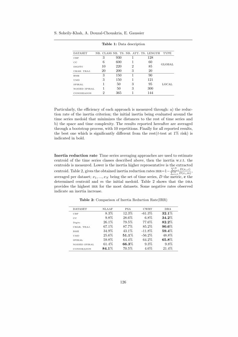
S. Soheily-Khah, A. Douzal-Chouakria, E. Gaussier
Table 1: Data description
dataset nb. class nb. ts. nb. att. ts. length type
CBF 3 930 1 128
globalCC 6 600 1 60DIGITS 10 220 2 85CHAR. TRAJ. 20 200 3 20
BME 3 150 1 90
localUMD 3 150 1 121SPIRAL 1 50 3 95NOISED SPIRAL 1 50 3 300CONSSEASON 2 365 1 144
Particularly, the efficiency of each approach is measured through: a) the reduc-tion rate of the inertia criterion; the initial inertia being evaluated around thetime series medoid that minimizes the distances to the rest of time series andb) the space and time complexity. The results reported hereafter are averagedthrough a bootstrap process, with 10 repetitions. Finally for all reported results,the best one which is significantly different from the rest(t-test at 1% risk) isindicated in bold.
Inertia reduction rate Time series averaging approaches are used to estimatecentroid of the time series classes described above, then the inertia w.r.t. thecentroids is measured. Lower is the inertia higher representative is the extracted
centroid. Table 2, gives the obtained inertia reduction rates irr=1−∑
N
i=1 D(xi,c)∑N
i=1 D(xi,m),
averaged per dataset; x1, ..., xN being the set of time series, D the metric, c thedetermined centroid and m the initial medoid. Table 2 shows that the dbaprovides the highest irr for the most datasets. Some negative rates observedindicate an inertia increase.
Table 2: Comparison of Inertia Reduction Rate(IRR)
dataset nlaaf psa cwrt dba
CBF 8.3% 12.3% -61.3% 32.1%CC 9.8% 28.6% 6.8% 34.2%Digits 26.1% 79.5% 77.6% 82.2%CHAR. TRAJ. 67.1% 87.7% 85.2% 90.6%BME 34.9% 43.1% -11.8% 59.4%UMD 25.6% 51.1% -56.2% 48.8%SPIRAL 59.8% 64.4% 64.2% 65.8%NOISED SPIRAL 61.4% 66.3% 9.3% 9.8%CONSSEASON 84.1% 70.5% 4.6% 21.4%
126

Progressive and Iterative Approaches for Time Series Averaging
Time and space complexity In Table 3 the studied approaches are comparedw.r.t their space and time complexity. The results, averaged per dataset, revealalmost dba the faster method and psa the slowest one. The cwrt approach isnot comparable to the rest of the methods as it performs directly an euclideandistance on the time series once the initial dtw matrix evaluated. Remark thatfor nlaaf and psa the centroid lengths are very large making these approachesunusable for large time series. The centroid lengths for the remaining methodsare equal to the length of the initial medoid. The higher time consumptionsobserved for nlaaf and psa are mainly explained by the progressive increase ofthe centroid length during the pairwise combination process.
Table 3: Comparison of Time/Space complexity
datasetnlaaf psa dba
length time length time length time(nb-it.)
CBF 8283 392.32 35042 9999.99 128 42.91(30)CC 992 4.15 1677 12.75 60 6.46(40)DIGITS 313 0.52 530 1.09 85 0.51(15)CHAR. TRAJ. 33 0.06 29 0.06 20 0.03(10)BME 2027 5.46 2781 11.92 90 3.93(30)UMD 2729 10.32 4280 28.87 121 4.75(30)SPIRAL 660 1.62 1122 3.33 95 1.19(10)NOISED SPIRAL 1699 16.13 9030 269.93 300 34.84(25)CONSSEASON 5741 77.10 32706 3680.81 144 29.79(35)
3.3 Discussion
From Table 2, we can see that dba and psa lead to the highest inertia reductionrates, where the best scores (indicated in bold) are reached by dba for almost alldatasets. However it is significantly lower for some challenging datasets. Finally,cwrt has the lowest inertia reduction rates. The negative rates observed forcwrt indicate an inertia increase. As expected, the dba method that iterativelyoptimizes an inertia criterion, in general, reaches higher values than the non-iterative methods (nlaaf, psa and cwrt).
From Table 3, the results reveal dba the fastest method and the psa theslowest one. For nlaaf and psa the estimated centroids have a drastically largedimension (i.e. a length around 104) making these approaches unusable for largetime series datasets. The nlaaf and psa methods are highly time-consuming,largely because of the progressive increase of the centroid length during the pair-wise combination process. The centroid lengths for the remaining methods areequal to the length of the initial medoid (Table 3). Finally, psa appears greatlyslower than nlaaf; this is due to the hierarchical clustering on the whole timeseries. We finally visualize here some of the centroids obtained by the differentmethods to compare their shape to the one of the time series they represent.
127

S. Soheily-Khah, A. Douzal-Chouakria, E. Gaussier
Figure (1) and (2) display the centroids obtained by the mentioned methodsrespectively for the class ”funnel” of cbf and ”cyclic” of data set cc. As onecan note, for global datasets, almost all the approaches succeed in obtaingingcentroids more or less similar to the initial time series. However, we observegenerally less representative centroids for nlaaf and psa.
Fig. 1: cbf-”funnel” centroids: (a) ground through, (b) nlaaf, (c) psa, (d) cwrt, (e) dba
Fig. 2: cc-”cyclic” centroids: (a) ground through, (b) nlaaf, (c) psa, (d) cwrt, (e) dba
4 Conclusion
The dtw is among the most frequently used metrics for time series in severaldomains as signal processing, temporal data analysis and mining or machinelearning. However, for time series clustering, approaches are generally limitedto kmedoid to circumvent time series averaging under dtw and tricky multipletemporal alignments problem. The present study compares the major progressiveand iterative time series averaging approaches under dynamic time warping. Theexperimental validation is based on global datasets in which time series sharesimilar behaviors within classes, as well as on more complex datasets exhibitingtime series that share only local characteristics, that are multidimensional andnoisy. Both the quantitative evaluation, based on an inertia criterion and timeand space complexity, and the qualitative one (consisting in the visualizationof the centroids obtained by different methods) show the effectiveness of dbaapproach. In particular, the dba method that iteratively optimizes an inertiacriterion, not only, reaches higher values than the non-iterative methods (nlaaf,psa and cwrt), but also provides a fast time series averaging for global and localdatasets.
References
1. Abdulla, W.H. and Chow, D. and Sin, G.: Cross-words reference template for DTW-based speech recognition systems. Proc. TENCON, Pages 1576–1579, Vol. 2 (2003)
2. Hautamaki, V. and Nykanen, P. and Franti, P.: Time-series clustering by approxi-mate prototypes. 19th International Conference on Pattern Recognition, (2008).
128

Progressive and Iterative Approaches for Time Series Averaging
3. Petitjean, F. and Ketterlin, A. and GanCarski, P.: A global averaging method fordynamic time warping, with applications to clustering. Pattern Recognition, Pages678-693, Vol. 44 (2011)
4. F. Zhou and F. De la Torre: Generalized time warping for multi-modal alignment ofhuman motion. IEEE, Computer Vision and Pattern Recognition (CVPR), Pages1282–1289 (2012)
5. Kruskall, J.B. and Liberman, M.: The symmetric time warping algorithm: Fromcontinuous to discrete. Addison-Wesley, Time Warps Journal (1983)
6. Sakoe, H. and Chiba, S.: Dynamic programming algorithm optimization for spokenword recognition. IEEE Transactions on Acoustics, Speech, and Signal Processing,Pages 43–49, Vol. 26 (1978)
7. Sankoff, D. and Kruskal, J.B.: Time warps, string edits, and macromolecules: thetheory and practice of sequence comparison. Cambridge University Press, Addison-Wesley, (1983)
8. Lalit Gupta, D. Molfese, R. Tammana, P. Simos: Nonlinear alignment and averagingfor estimating the evoked potential. IEEE T. on Biomedical Engineering, No. 4,Pages 348–356, Vol. 43 (1996)
9. C. Frambourg, A. Douzal-Chouakria and E. Gaussier: Learning Multiple TemporalMatching for Time Series Classification. In Advances in Intelligent Data AnalysisXII (pp. 198-209). Springer Berlin Heidelberg. (2013)
10. UCI Machine Learning Repository, ”http://archive.ics.uci.edu/ml/ ”11. V. Niennattrakul, C. Ratanamahatana: On Clustering Multimedia Time Series
Data Using K-means and Dynamic Time Warping. Multimedia and Ubiquitous En-gineering, MUE’07. International Conference on IEEE, Pages 733–738, (2007)
12. V. Niennattrakul, C. Ratanamahatana: Shape Averaging under Time Warping.Electrical Engineering/Electronics, Computer, Telecommunications and Informa-tion Technology, ECTI-CON 6th International Conference on IEEE, Vol. 2, Pages626–629, May (2009)
129

130

Proceedings 1st International Workshop on Advanced Analytics and Learning on Temporal DataAALTD 2015
Classification Factored Gated
Restricted Boltzmann Machine
Ivan SorokinITMO University, Department of Secure Information Technology,
9 Lomonosova str., St. Petersburg, 191002, [email protected]
Abstract. Factored gated restricted Boltzmann machine is a generativemodel, which capable to extract the transformation from an image pair.We extend this model by adding discriminative component, which allowsdirectly use this model as a classifier, instead of using the hidden unitresponses as features for another learning algorithm. To evaluate thecapabilities of this model, we have created a synthetically transformedimage pairs and demonstrated that the model is able to determine thevelocity of object presented on two consecutive images.
Keywords: Multiplicative interaction, temporal coherence, translationalmotion, gated Boltzmann machine, supervision learning
1 Introduction
The gated Boltzmann machine is one of the models that uses multiplicative in-
teractions [8] for learning the representation, which can be useful to extract thetransformation between pairs of temporally coherent video frames [12]. Factor-ized version of this model is presented in [9], where authors train the model onshifts of random dot images and demonstrate that the model is able to identifythe different directions correctly. We continue this research by studying the pos-sibility to predict not only directions, but also a shift value. From all types ofmotion, we chose only translational motion, because it gives a great opportunityto use this model in many vision tasks, such as object tracking or visual odom-etry [4]. Therefore, the main objective of this work is to create a model that istrained to identify velocity vector in the image coordinate.
Instead of using additional model on top of the mapping units, we are addingdiscriminative component directly to the model. This technique was first appliedfor restricted Boltzmann machine [6] and since that has become widely used forsimilar models [11, 10]. In this paper, we are focused on the model that extractstransformation from two consecutive images. Without considering the additionaldiscriminative component, there are several approaches of three-way structuremodel training [9, 13]. We propose a simple learning algorithm and show thatit is not inferior to the existing. Moreover, our learning algorithm takes intoaccount additional label variables and we demonstrate how it effects the trainingdiscriminative features. We refer to our model variants as classification factored
gated restricted Boltzmann machine (cfgRBM).
Copyright c©2015 for this paper by its authors. Copying permitted for private and academicpurposes.
131

I. Sorokin
Fig. 1. Left shows the schematic representation of the cfgRBM model. Factorized formof the multiplicative interactions between two visible x, y and hidden h vectors de-picted by triangles. The discriminative component is presented as one-hot encodedlabel vector z. Right shows specially chosen four filter pairs learned on horizontallyshifted handwritten digits.
2 The Model
We propose a model (Fig. 1) in which the hidden units h not only capturesthe relationship between two images x and y, but also interacts with associatedlabel z. The model is defined in the terms of its energy function and the functionconsists of two basic parts. The first of these is the factored three-way Boltzmannmachine [13] and the second is classification restricted Boltzmann machine [5].Combining these two models we defined expression for the energy function asfollows:
E(x, y, z, h) = −∑
f
(∑
i
W xifxi)(
∑
j
Wyjfyj)(
∑
k
Whkfhk)−
∑
kl
hkVklzl
−∑
i
aixi −∑
j
bjyj −∑
k
ckhk −∑
l
dlzl , (1)
where matrices W x,W y,Wh has size I×F, J×F and K×F respectively, I andJ are equal size of visible units, F - number of factors, K - number of hiddenunits. The discriminative component is weight matrix V with size K × L andone-hot encoded label vector z with L classes. Bias terms a, b, c and d associatedwith two visible, hidden and label vectors respectively. We will assume that thevisible vectors are binary, but the model can be defined with real-valued units[1]. Every column W x
·f and Wy·f can be consider as filter pairs (Fig. 1).
To train the model, we also need to define the joint probability distributionover three vectors:
p(x, y, z) =
∑
h exp(−E(x, y, z, h))∑
x,y,z,h exp(−E(x, y, z, h)), (2)
where the numerator is summing over all possible hidden vectors and denomi-nator is partition function which cannot be efficiently approximated.
132

Classification Factored Gated Restricted Boltzmann Machine
2.1 Inference
The inference task of proposed model is defined as the problem of classifyingthe motion between two related images. In order to choose the most probablelabel under this model, we must compute conditional distribution p(z|x, y). Wehave adapted the calculations from the case of single input units [5] for the caseof three-way interaction. As a result, for reasonable numbers of labels L, thisconditional distribution can be also computed exactly and efficiently, by writingit as follows:
p(zl = 1 | x,y) =exp(dl)
∏
k (1 + exp(okl(x,y)))∑
l∗ exp(dl∗)∏
k (1 + exp(okl∗(x,y))), (3)
whereokl(x,y) = ck + Vkl +
∑
f
Whkf (W
x·f
⊤x)(W y
·f⊤y) (4)
is an input to k hidden unit received from images x, y and estimated label l.
2.2 Learning
In order to train a cfgRBM to solve a classification problem, we need to learn themodel parameters Θ = (W x,W y,Wh, V, a, b, c, d). Given a training set Dtrain =(xα, yα, zα) and a predefined joint distribution (2) between three variables,the model can be trained by minimizing the negative log-likelihood:
Lgen(Dtrain) = −
|Dtrain|∑
a=1
log p(xα, yα, zα) . (5)
In order to minimize this function the gradient for any cfgRBM parametersθ ∈ Θ can be written as follows:
−Eh|xα,yα,zα
[
∂E(xα, yα, zα, h)
∂θ
]
+ Ex,y,z,h
[
∂E(x, y, z, h)
∂θ
]
, (6)
where subscript of the expectation denotes the distribution for variables. Thereexists a learning rule [2], called “Contrastive Divergence”, which can be usedto approximate this gradient. Taking this rule into consideration we proposedthe Algorithm 1 for the training of cfgRBM model. The main difference fromthe other approaches for training three-way interaction is in symmetrically sam-ple vectors x,y in the negative phase. Detailed information about the partialderivatives with respect to the model parameters can be obtained from [9, 5].
In case of factored three-way interactions the calculation of the gradient (6)involves numerical instabilities. Especially when using a large input vectors. Toavoid this we also use a norm constraint on columns of matrics W x and W y. Itis a common approach to stabilizing learning. For example, the same recommen-dations are given by [3] for method “Adaptive Subspace Self-Organizing Map”to learn invariant properties of moving input patterns.
133
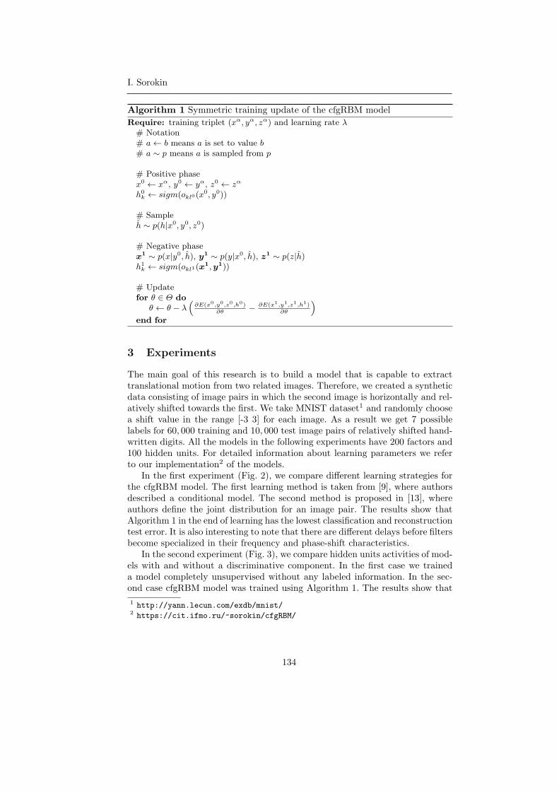
I. Sorokin
Algorithm 1 Symmetric training update of the cfgRBM model
Require: training triplet (xα, yα, zα) and learning rate λ
# Notation# a← b means a is set to value b
# a ∼ p means a is sampled from p
# Positive phasex0 ← xα, y0 ← yα, z0 ← zα
h0k ← sigm(okl0(x
0, y0))
# Sampleh ∼ p(h|x0, y0, z0)
# Negative phasex
1 ∼ p(x|y0, h), y1 ∼ p(y|x0, h), z1 ∼ p(z|h)h1k ← sigm(okl1(x
1,y1))
# Updatefor θ ∈ Θ do
θ ← θ − λ(
∂E(x0,y0,z0,h0)∂θ
− ∂E(x1,y1,z1,h1)∂θ
)
end for
3 Experiments
The main goal of this research is to build a model that is capable to extracttranslational motion from two related images. Therefore, we created a syntheticdata consisting of image pairs in which the second image is horizontally and rel-atively shifted towards the first. We take MNIST dataset1 and randomly choosea shift value in the range [-3 3] for each image. As a result we get 7 possiblelabels for 60, 000 training and 10, 000 test image pairs of relatively shifted hand-written digits. All the models in the following experiments have 200 factors and100 hidden units. For detailed information about learning parameters we referto our implementation2 of the models.
In the first experiment (Fig. 2), we compare different learning strategies forthe cfgRBM model. The first learning method is taken from [9], where authorsdescribed a conditional model. The second method is proposed in [13], whereauthors define the joint distribution for an image pair. The results show thatAlgorithm 1 in the end of learning has the lowest classification and reconstructiontest error. It is also interesting to note that there are different delays before filtersbecome specialized in their frequency and phase-shift characteristics.
In the second experiment (Fig. 3), we compare hidden units activities of mod-els with and without a discriminative component. In the first case we traineda model completely unsupervised without any labeled information. In the sec-ond case cfgRBM model was trained using Algorithm 1. The results show that
1 http://yann.lecun.com/exdb/mnist/2 https://cit.ifmo.ru/~sorokin/cfgRBM/
134

Classification Factored Gated Restricted Boltzmann Machine
descriminative component has a strong effect on hidden features. In addition,we also demonstrate an effect on the hidden units in the case with wrong labelinformation.
Fig. 2. Three learning stratagies for cfgRBM model. The reconstruction was calculatedonly for y visible units. In both graphs the error value obtained on test set and theordinate is scaled logarithmically. Best view in color.
Fig. 3. Hidden units activations. For every test sample, activation of 100 hidden unitsprojected to 2D coordinates using t-SNE [7]. a) model trained without discriminativecomponent. b) model extendet with additional labeled units. c) exactly the same modelas in the case (b), but labels of classes -3,-2 and 2,3 are deliberetly combined.
135

I. Sorokin
4 Conclusion
In this paper, we incorporate supervision learning for factored gated restrictedBoltzmann machine model. Our results show that proposed model is capable toidentify the velocity of the object presented on two consecutive images. In thefuture work we plan to apply this model for videos which may be representedas a temporally ordered sequence of images. Particularly, the ability to extracttranslational motion will be useful for tracking tasks.
References
1. Fischer, A., Igel, C.: Training restricted Boltzmann machines: an introduction. Pat-tern Recognition 47(1), pp. 25–39 (2014)
2. Hinton, G.: Training products of experts by minimizing contrastive divergence. Neu-ral computation 14, pp. 1771-1800 (2002)
3. Kohonen, T.: The adaptive-subspace som (assom) and its use for the implementationof invariant feature detection. In: Proc. ICANN95, Int. Conf. on Artificial NeuralNetworks, pp. 3-10 (1995)
4. Konda, K., Memisevic, R.: Learning visual odometry with a convolutional network.International Conference on Computer Vision Theory and Applications. (2015)
5. Larochelle, H., Mandel, M., Pascanu, R., Bengio, Y.: Learning algorithms for theclassification restricted boltzmann machine. Journal of Machine Learning Research13, pp. 643-669 (2012)
6. Larochelle, H., Bengio, Y.: Classification using discriminative restricted Boltzmannmachines. In: Proceedings of the 25th international conference on Machine learning,pp. 536–543 (2008)
7. Van der Maaten, L., Hinton, G.: Visualizing data using t-sne. Journal of MachineLearning Research 9, pp. 2579–2605 (2008)
8. Memisevic, R.: Learning to relate images. IEEE Transactions on Pattern Analysisand Machine Intelligence 35, pp. 1829-1846 (2013)
9. Memisevic, R., Hinton, G.E.: Learning to represent spatial transformations withfactored higher-order boltzmann machines. Neural Computation 22, pp. 1473-1492(2010)
10. Reed, S., Sohn, K., Zhang, Y., Lee, H.: Learning to disentangle factors of variationwith manifold interaction. In: Proceedings of the 31st International Conference onMachine Learning, pp. 1431-1439 (2014)
11. Sohn, K., Zhou, G., Lee, C., Lee, H.: Learning and selecting features jointly withpoint-wise gated boltzmann machines. In: Proceedings of The 30th InternationalConference on Machine Learning, pp. 217-225 (2013)
12. Srivastava, N.: Unsupervised Learning of Visual Representations using Videos.Department of Computer Science, University of Toronto. Technical Report. (2015)Retrived from http://www.cs.toronto.edu/~nitish/depth_oral.pdf
13. Susskind, J., Memisevic, R., Hinton, G., Pollefeys, M.: Modeling the joint density oftwo images under a variety of transformations. In: Proceedings of IEEE Conferenceon Computer Vision and Pattern Recognition, pp. 2793-2800 (2011)
136

Index of Authors
Amsaleg, L. p. 71 Lafuente-Rego, B.R. p. 93Andrade-Pacheco, R. p. 3 Lagacherie, M. p. 109Bailly, A. p. 11 Lawrence, N. p. 3Billard, L. p. 19 Maby, S. p. 109Bondu, A. p. 27 Malinowski, S. p. 11, 71Boulle, M. p. 27 Marie, S. p. 39Camps-Valls, G. p. 1 Marteau, P.-F. p. 47Cattuto, C. p. 117 Micheli, A. p. 57Chapel, L p. 11 Mubangizi, M. p. 3Cornuejols, A. p. 27 Nelson, J.D.B. p. 63Cubille, J. p. 109 Panisson, A. p. 117Do, C.-T. p. 39 Parodi, O. p. 57Douzal-Chouakria, A. p. 19, 39, 123 Pedrelli, L. p. 57Dupont, M. p. 47 Quiniou, R. p. 71Gallicchio, C. p. 57 Quinn, J. p. 3Gaussier, E. p. 123 Rahmadi, R. p. 101Gauvin, L. p. 117 Rombaut, M. p. 39Gibberd, A.J. p. 63 Salperwyck, C. p. 109Gravier, G. p. 71 Samadi, S.Y. p. 19Groot, P. p. 101 Sapienza, A. p. 117Guyet, T. p. 11 Soheily-Khah, S. p. 123Hardy, C. p. 71 Sorokin, I. p. 131Heins, M. p. 101 Spiegel, S. p. 79Heskes, T. p. 101 Tavenard, R. p. 11Jain, B.J. p. 79 Vilar, J.A. p. 93Knoop, H. p. 101 Vozzi, F. p. 57Krempl, G. p. 85 Wu, J. p. 117
137