Proceedings of the 2013 Uncertainty in Arti cial ...ceur-ws.org/Vol-1024/UAI2013AW2013-complete.pdf · Preface The Uncertainty in Artiﬁcial Intelligence (UAI) Application Workshop

Proceedings of the 2013 Uncertainty in Artificial

Intelligence Application Workshops:

Part I: Big Data meet Complex Models

and

Part II: Spatial, Temporal, and Network Models

Workshops took place on July 15, 2013, in Bellevue,Washington, USA.

Edited byRussell G. Almond, Florida State University

andOle J. Mengshoel, Carnegie Mellon University

CEUR Workshop Proceedings, Vol. 1024http://ceur-ww.org/Vol-1024/

Copyright c© 2013 for the individual papers by the papers’ authors. Copying permittedonly for private and academic purposes. This volume is published and copyrighted byits editors.

Preface

The Uncertainty in Artificial Intelligence (UAI) Application Workshop was conceived in 2002, and first heldat UAI 2003 in Acapulco, Mexico; the first time a workshop was associated with the Conference. This yearmarks the Workshop’s tenth anniversary, having been held in all years since but 2010. The goal of theworkshops has been and will continue to be to look at the practical issues that arise in fielding applicationsbased on the methods explored in the main conference.

Two half-day application Workshops where held on July 15, 2013 in Bellevue, Washington, USA, afterthe main UAI 2013 conference, along with two other workshops on specific topics. This volume collects thepapers from both application workshops.

Application Workshop I: Big Data meet Complex Models

The theme of this workshop was large data sets containing many different kinds of data, and it especiallyemphasized the procedures that are used to combine data from various sources as part of the modelingprocess. There were 9 submissions. Each submission was reviewed by at least 1, and on the average 2.8program committee members. The committee decided to accept 6 papers. Because one paper containedreferences to proprietary information, one set of authors published only the abstract in this volume.

Application Workshop II: Spatial, Temporal, and Network Models

The theme of this workshop was spatial, temporal, and network data. One may be interested in consideringuncertainty in mobile data, generated by a GPS-enabled phone or a car. Another example is this: A scientistdevelops a probabilistic model in the form of a Bayesian network or a Markov random field. A computerscientist or computer engineer is then concerned about how to efficiently compile and execute the model inorder to compute posterior distributions or estimate parameters on a multi-core CPU, a GPU, a Hadoopcluster, or a supercomputer. How well has this model worked, and what are current challenges and oppor-tunities? There were 7 submissions. Each submission was reviewed by 3 program committee members. Thecommittee decided to accept 5 papers, and all of these are being published in this volume.

Thanks to the program committees who put up with all of our nagging, and to all of the authors whocame to us with a wide variety different applications, making the job of reading the papers much moreinteresting. Special thanks to John Mark Agosta of Toyota-ITC who as the UAI Workshop Chair (and pastApplications Workshop Chair) helped us work out many details; and to Marina Meila of the University ofWashington, who handled the local arrangements for us. Thanks also to EasyChair.org for helping with thesubmission and review process, to the volunteers who created the ceur-make facility for helping with theproceedings, and the people at CEUR for hosting our final papers.

Finally, thanks to the Association for Uncertainty in Artificial Intelligence (http://auai.org/) for host-ing this workshop.

July 15, 2013Bellevue, Washington, USA

Russell G. Almond and Ole J. Mengshoel

Program Committee


Russell Almond Florida State UniversityMarek Druzdzel University of PittsburgJulia Flores Universidad de Castilla-La ManchaLionel Jouffe Bayesia SASKathryn Laskey George Mason UniversitySuzanne Mahoney Innovative DecisionsThomas O’Neil The American Board of Family MedicineLinda van der Gaag Utrecht UniversityAdditional ReviewersBermejo, PabloMartınez, Ana Marıa

Part II: Models for Spatial, Temporal, and Network Data

Dennis Buede Innovative DecisionsAsela Gunawardana MicrosoftJennifer Healey IntelOscar Kipersztok BoeingBranislav Kveton TechnicolorHelge Langseth Norwegian University of Science and TechnologyOle Mengshoel Carnegie Mellon UniversityTomas Singliar BoeingEnrique Sucar Instituto Nacional de Astrofisica Optica y Electronica, MexicoTom Walsh Massachusetts Institute of Technology

Table of Contents


Debugging the Evidence Chain . . . . . . . . . . . . . . . . . . . . . . . . . . . . . . . . . . . . . 1Russell Almond, Yoon Jeon Kim, Valerie Shute and Matthew Ventura

Bayesian Supervised Dictionary learning . . . . . . . . . . . . . . . . . . . . . . . . . . . . . 11Behnam Babagholami-Mohamadabadi, Amin Jourabloo, MohammadrezaZolfaghari and Mohammad. T Manzuri-Shalmani

Identifying Learning Trajectories in an Educational Video Game . . . . . . . . 20Deirdre Kerr and Gregory K.W.K. Chung

Transforming Personal Artifacts into Probabilistic Narratives . . . . . . . . . . . 29Setareh Rafatirad and Kathryn Laskey

Learning Parameters by Prediction Markets and Kelly Rule forGraphical Models . . . . . . . . . . . . . . . . . . . . . . . . . . . . . . . . . . . . . . . . . . . . . . . . . 39

Wei Sun, Robin Hanson, Kathryn Laskey and Charles Twardy

Predicting Latent Variables with Knowledge and Data: A Case Studyin Trauma Care . . . . . . . . . . . . . . . . . . . . . . . . . . . . . . . . . . . . . . . . . . . . . . . . . . . 49

Barbaros Yet, William Marsh, Zane Perkins, Nigel Tai and NormanFenton

Part II: Models for Spatial, Temporal, and Network Data

A lightweight inference method for image classification . . . . . . . . . . . . . . . . . 50John Agosta and Preeti Pillai

Product Trees for Gaussian Process Covariance in Sublinear Time . . . . . . . 58David A. Moore and Stuart Russell

Latent Topic Analysis for Predicting Group Purchasing Behavior onthe Social Web . . . . . . . . . . . . . . . . . . . . . . . . . . . . . . . . . . . . . . . . . . . . . . . . . . . 67

Feng-Tso Sun, Yi-Ting Yeh, Ole Mengshoel and Martin Griss

An Object-oriented Spatial and Temporal Bayesian Network forManaging Willows in an American Heritage River Catchment . . . . . . . . . . 77

Lauchlin A.T. Wilkinson, Yung En Chee, Ann Nicholson and PedroQuintana-Ascencio

Exploring Multiple Dimensions of Parallelism in Junction Tree MessagePassing . . . . . . . . . . . . . . . . . . . . . . . . . . . . . . . . . . . . . . . . . . . . . . . . . . . . . . . . . . 87

Lu Zheng and Ole Mengshoel

Debugging the Evidence Chain

Russell G. Almond∗

Florida State UniversityYoon Jeon Kim

Florida State UniversityValerie J. Shute

Florida State UniversityMatthew Ventura

Florida State University

Abstract

In Education (as in many other fields) it iscommon to create complex systems to as-sess the state of latent properties of indi-viduals — the knowledge, skills, and abili-ties of the students. Such systems usuallyconsist of several processes including (1) acontext determination process which identi-fies (or creates) tasks—contexts in which evi-dence can be gathered,—(2) an evidence cap-ture process which records the work productproduced by the student interacting with thetask, (3) an evidence identification processwhich captures observable outcome variablesbelieved to have evidentiary value, and (4)an evidence accumulation system which in-tegrates evidence across multiple tasks (con-texts), which often can be implemented us-ing a Bayesian network. In such systems,flaws may be present in the conceptualiza-tion, identification of requirements or imple-mentation of any one of the processes. Inlater stages of development, bugs are usu-ally associated with a particular task. Taskswhich have exceptionally high or unexpect-edly low information associated with theirobservable variables may be problematic andmerit further investigation. This paper iden-tifies individuals with unexpectedly high orlow scores and uses weight-of-evidence bal-ance sheets to identify problematic tasks forfollow-up. We illustrate these techniqueswith work on the game Newton’s Playground :an educational game designed to assess a stu-dent’s understanding of qualitative physics.

∗Paper submitted to Big Data Meets Complex Models, Applica-

tion Workshop at Uncertainty in Artificial Intelligence Conference2013, Seattle, WA.

Key words: Bayesian Networks, Model Construction,Mutual Information, Weight of Information, Debug-ging

1 Introduction

The primary goal of educational assessment is to drawinferences about the unobservable pattern of studentknowledge, skills and abilities from a pattern of ob-served behaviors in recognized contexts. The reason-ing chain of an assessment system has several links:(1) It must recognize that the student has entered acontext where evidence can be gathered (often, this isdone by providing the student with a problem that pro-vides the assessment context). We call such a context atask, as frequently it is the task of solving the problemwhich provides the required evidence. (2) The rele-vant parts of the student’s performance on that task,the student’s work product, must be captured. (3) Thework product is then distilled into a series of observ-able outcome variables. (4) These observable outcomevariables are used to update beliefs about the latentproficiency variables which are the targets of interest.

Bayesian networks are well suited for the fourth linkin the evidentiary chain. Often the network can bedesigned to have a favorable topology, where observ-able variables from different contexts are conditionallyindependent given the latent proficiency variables. Insuch cases, the Bayesian network can be partitionedinto a student proficiency model—containing only thelatent proficiency variables—and a series of evidencemodels (one for each task)—capturing the relation-ships between the proficiency and evidence models fora particular task (Almond & Mislevy, 1999).

When the assessment system does not perform as ex-pected, there is still a model with hundreds of vari-ables that must be debugged. Furthermore, the prob-lem may not lie just in the Bayesian network, the lastlink of the evidentiary chain, but anywhere along thatchain. By using various information metrics, the prob-

1

lem can be traced to the parts of the evidentiary chainassociated with a particular tasks. In particular, if theanomalous behavior can be associated with a partic-ular individual attempting a particular task, this canfocus troubleshooting effort to places where it is likelyto provide the most value.

This paper explores the use of information metrics introubleshooting the assessment system embedded inthe game Newton’s Playground(NP ; Section 2). Sec-tion 3 describes a generic four process architecture foran assessment system. In NP tasks correspond togame levels; Section 4 describes some information met-rics used to identify problematic game levels. Section 5describes some of the problem identified so far, and ourfuture development and model refinement plans.

2 Newton’s Playground

Shute, Ventura, Bauer, and Zapata-Rivera (2009) ex-plores the idea that if an assessment system can beembedded in an activity that students find pleasur-able (e.g., a digital game), and that the activity re-quires them exercise a skill that educators care about(e.g., knowledge of Newton’s laws of motion), then byobserving performance in that activity, educators canmake unobtrusive assessment of the students abilitywhich can be used to guide future instruction. New-tons Playground (Shute & Ventura, 2013) is a two-dimensional physics game, inspired by the commercialgame Crayon Physics Deluxe. It is also designed to bean assessment of three different aspects of proficiency:qualitative physics (Ploetzner & VanLehn, 1997), per-sistence, and creativity. This paper focuses on assess-ment of qualitative physics proficiency.

2.1 Gameplay

NP is divided into a series of levels, where each levelconsists of a qualitative physics problem to solve. Ineach game level, the player is presented with a draw-ing containing both fixed and movable objects. Thegoal of the level is to move the ball to a balloon (thetarget), by drawing additional objects on the screen.Most objects (both drawn and preexisting) are sub-ject to the laws of gravity (with the exception of somefixed background objects) and Newton’s laws of mo-tion. (The open source Box 2D (Catto, 2011) physicsengine provides the physics simulation.)

Figure 1 shows the initial configuration of a typicallevel called Spider’s Web. Figure 2 shows one possiblesolution in which the player has used a springboard(attached to the ledge with two pins—small round cir-cles) to provide energy to propel the ball up to the bal-loon. Deleting the weight will cause the ball to strike

Figure 1: Starting Position for Spider Web Level

Figure 2: Spider Web Level with Springboard Solu-tion.

ramp attached to the top of the wall which keeps theball from flying over the target.

The focus of the current version has been on fouragents of motion (simple machines): ramps, levers,springboards and pendulums. The game engine de-tects when one of those four agents was used as partof the solution. The game awards a trophy when theplayer solves a game level. Gold trophies are awardedif the solution is efficient (uses few drawn objects) andsilver trophies are given as long as the goal is reached.

2.2 Proficiency and Evidence Models

The yellow nodes in Figure 3 show the student pro-ficiency model for assessing a player’s qualitativephysics understanding. The highest level node, New-ton’s Three Laws, is the target of inference. It is di-vided into two components: one related to the applica-tion of those laws in linear motion, and one in angular

2

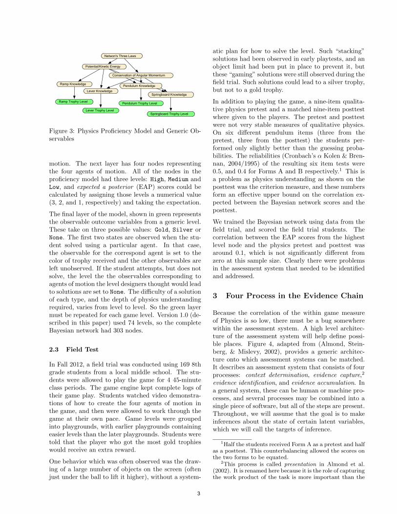
Figure 3: Physics Proficiency Model and Generic Ob-servables

motion. The next layer has four nodes representingthe four agents of motion. All of the nodes in theproficiency model had three levels: High, Medium andLow, and expected a posterior (EAP) scores could becalculated by assigning those levels a numerical value(3, 2, and 1, respectively) and taking the expectation.

The final layer of the model, shown in green representsthe observable outcome variables from a generic level.These take on three possible values: Gold, Silver orNone. The first two states are observed when the stu-dent solved using a particular agent. In that case,the observable for the correspond agent is set to thecolor of trophy received and the other observables areleft unobserved. If the student attempts, but does notsolve, the level the the observables corresponding toagents of motion the level designers thought would leadto solutions are set to None. The difficulty of a solutionof each type, and the depth of physics understandingrequired, varies from level to level. So the green layermust be repeated for each game level. Version 1.0 (de-scribed in this paper) used 74 levels, so the completeBayesian network had 303 nodes.

2.3 Field Test

In Fall 2012, a field trial was conducted using 169 8thgrade students from a local middle school. The stu-dents were allowed to play the game for 4 45-minuteclass periods. The game engine kept complete logs oftheir game play. Students watched video demonstra-tions of how to create the four agents of motion inthe game, and then were allowed to work through thegame at their own pace. Game levels were groupedinto playgrounds, with earlier playgrounds containingeasier levels than the later playgrounds. Students weretold that the player who got the most gold trophieswould receive an extra reward.

One behavior which was often observed was the draw-ing of a large number of objects on the screen (oftenjust under the ball to lift it higher), without a system-

atic plan for how to solve the level. Such “stacking”solutions had been observed in early playtests, and anobject limit had been put in place to prevent it, butthese “gaming” solutions were still observed during thefield trial. Such solutions could lead to a silver trophy,but not to a gold trophy.

In addition to playing the game, a nine-item qualita-tive physics pretest and a matched nine-item posttestwhere given to the players. The pretest and posttestwere not very stable measures of qualitative physics.On six different pendulum items (three from thepretest, three from the posttest) the students per-formed only slightly better than the guessing proba-bilities. The reliabilities (Cronbach’s α Kolen & Bren-nan, 2004/1995) of the resulting six item tests were0.5, and 0.4 for Forms A and B respectively.1 This isa problem as physics understanding as shown on theposttest was the criterion measure, and these numbersform an effective upper bound on the correlation ex-pected between the Bayesian network scores and theposttest.

We trained the Bayesian network using data from thefield trial, and scored the field trial students. Thecorrelation between the EAP scores from the highestlevel node and the physics pretest and posttest wasaround 0.1, which is not significantly different fromzero at this sample size. Clearly there were problemsin the assessment system that needed to be identifiedand addressed.

3 Four Process in the Evidence Chain

Because the correlation of the within game measureof Physics is so low, there must be a bug somewherewithin the assessment system. A high level architec-ture of the assessment system will help define possi-ble places. Figure 4, adapted from (Almond, Stein-berg, & Mislevy, 2002), provides a generic architec-ture onto which assessment systems can be matched.It describes an assessment system that consists of fourprocesses: context determination, evidence capture,2

evidence identification, and evidence accumulation. Ina general system, these can be human or machine pro-cesses, and several processes may be combined into asingle piece of software, but all of the steps are present.Throughout, we will assume that the goal is to makeinferences about the state of certain latent variables,which we will call the targets of inference.

1Half the students received Form A as a pretest and halfas a posttest. This counterbalancing allowed the scores onthe two forms to be equated.

2This process is called presentation in Almond et al.(2002). It is renamed here because it is the role of capturingthe work product of the task is more important than the

3

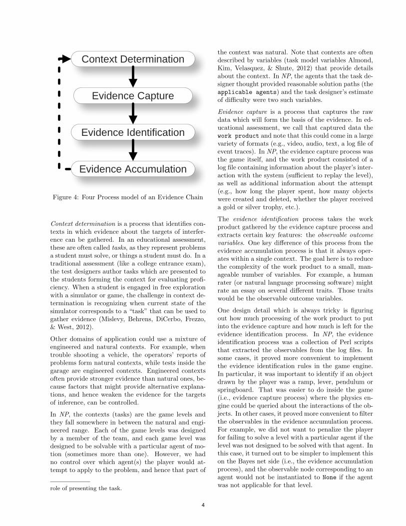
Context Determination

Evidence Identification

Evidence Accumulation

Evidence Capture

Figure 4: Four Process model of an Evidence Chain

Context determination is a process that identifies con-texts in which evidence about the targets of interfer-ence can be gathered. In an educational assessment,these are often called tasks, as they represent problemsa student must solve, or things a student must do. In atraditional assessment (like a college entrance exam),the test designers author tasks which are presented tothe students forming the context for evaluating profi-ciency. When a student is engaged in free explorationwith a simulator or game, the challenge in context de-termination is recognizing when current state of thesimulator corresponds to a “task” that can be used togather evidence (Mislevy, Behrens, DiCerbo, Frezzo,& West, 2012).

Other domains of application could use a mixture ofengineered and natural contexts. For example, whentrouble shooting a vehicle, the operators’ reports ofproblems form natural contexts, while tests inside thegarage are engineered contexts. Engineered contextsoften provide stronger evidence than natural ones, be-cause factors that might provide alternative explana-tions, and hence weaken the evidence for the targetsof inference, can be controlled.

In NP, the contexts (tasks) are the game levels andthey fall somewhere in between the natural and engi-neered range. Each of the game levels was designedby a member of the team, and each game level wasdesigned to be solvable with a particular agent of mo-tion (sometimes more than one). However, we hadno control over which agent(s) the player would at-tempt to apply to the problem, and hence that part of

role of presenting the task.

the context was natural. Note that contexts are oftendescribed by variables (task model variables Almond,Kim, Velasquez, & Shute, 2012) that provide detailsabout the context. In NP, the agents that the task de-signer thought provided reasonable solution paths (theapplicable agents) and the task designer’s estimateof difficulty were two such variables.

Evidence capture is a process that captures the rawdata which will form the basis of the evidence. In ed-ucational assessment, we call that captured data thework product and note that this could come in a largevariety of formats (e.g., video, audio, text, a log file ofevent traces). In NP, the evidence capture process wasthe game itself, and the work product consisted of alog file containing information about the player’s inter-action with the system (sufficient to replay the level),as well as additional information about the attempt(e.g., how long the player spent, how many objectswere created and deleted, whether the player receiveda gold or silver trophy, etc.).

The evidence identification process takes the workproduct gathered by the evidence capture process andextracts certain key features: the observable outcomevariables. One key difference of this process from theevidence accumulation process is that it always oper-ates within a single context. The goal here is to reducethe complexity of the work product to a small, man-ageable number of variables. For example, a humanrater (or natural language processing software) mightrate an essay on several different traits. Those traitswould be the observable outcome variables.

One design detail which is always tricky is figuringout how much processing of the work product to putinto the evidence capture and how much is left for theevidence identification process. In NP, the evidenceidentification process was a collection of Perl scriptsthat extracted the observables from the log files. Insome cases, it proved more convenient to implementthe evidence identification rules in the game engine.In particular, it was important to identify if an objectdrawn by the player was a ramp, lever, pendulum orspringboard. That was easier to do inside the game(i.e., evidence capture process) where the physics en-gine could be queried about the interactions of the ob-jects. In other cases, it proved more convenient to filterthe observables in the evidence accumulation process.For example, we did not want to penalize the playerfor failing to solve a level with a particular agent if thelevel was not designed to be solved with that agent. Inthis case, it turned out to be simpler to implement thison the Bayes net side (i.e., the evidence accumulationprocess), and the observable node corresponding to anagent would not be instantiated to None if the agentwas not applicable for that level.

4

The Evidence accumulation process is responsible forcombining evidence about the targets of inferenceacross multiple contexts. In NP, the evidence accu-mulation process consisted of a collection of Bayesiannetworks: a student proficiency model for each stu-dent, and a collection of evidence models for each gamelevel. When it received a vector of observables for aparticular student on a particular game level, it drewthe appropriate evidence model from the library andattached it to that student’s proficiency model. It theninstantiated nodes in the evidence model correspond-ing to the observable values, and propagated the evi-dence into the proficiency model. The evidence modelwas then detached from the proficiency model whichremained as a record of student proficiency. It couldbe queried at any time to provide a score for a student(Almond, Shute, Underwood, & Zapata-Rivera, 2009).

The dashed line in Figure 4 from the evidence accumu-lation process to the context determination process3

is to indicate that in some situations the context de-termination might query the current beliefs about thetargets of inference before selecting the next task (con-text). This produces a system that is adaptive (Shute,Hansen, & Almond, 2008). In NP, the player was freeto choose the order for attempting the levels, hencethis link was not used.

The four processes can be put together into a systemthat provides real-time inference or as a series of iso-lated steps. In version 1.0 of NP, only the evidencecapture system (the game itself) was presented to theplayers in real-time. As the design of the other partsof the system was still undergoing refinement, it wassimpler to implement them as separate post-processingsteps. In a future version, these process will be inte-grated with the game so that players can get scoresfrom the Bayes net as they are playing.

Developing each process requires three activities: con-ceptualization—identifying the key variables and workproducts and their relationships,—requirement speci-fications—writing down the rules by which values ofthe variables are determined,—and implementation—realizing those rules in code. A bug that causes thesystem to behave poorly can be related to a flaw inany one of those three activities, and can affect one ormore of the four processes.

By the time the system was field tested, obvious bugshad been found and fixed. The remaining bugs onlyoccur in particular particular game levels, and partic-ular patterns of interaction with those levels. Oncethe levels in which bugs manifest and the patterns ofusage which cause the bugs to manifest are identified,

3Almond et al. (2002) called this the activity selectionprocess, to emphasize its adaptive nature.

the problems can be addressed. This may entail adjustparameters for the Bayesian network fragment associ-ated with that network, changing the level, replacingthe level or making changes to the game engine, evi-dence identification scripts, or instructions to players.

4 Information Metrics as DebuggingTools

It is always the case that students interacting with anassessment system do so in ways that were unantici-pated by the assessment designers. Information met-rics provide a mechanism for flagging levels which be-have in unexpected ways. In particular, we expect thata properly working game level will provide high infor-mation for the applicable agents (the ones that thedesigners targeted) and low information for the inap-plicable agents. Extremely high information could alsobe an indication of overfitting the model to data.

Section 4.1 looks at the parameters of the conditionalprobability table as information metrics. Section 4.2looks at the mutual information between the observ-able variable and its immediate parent in the model.Section 4.3 looks at tracing the score of specific in-dividuals as they work through the game to identifyproblematic player/level combinations.

4.1 Parameters of the ConditionalProbability Tables

Following Almond et al. (2001) and Almond (2010), weused models based on item response theory (IRT) todetermine the values of the conditional probability ta-bles. For each table, the effective ability parameter, θ,is determined by the value of the parent variable (thevalues were selected based on equally spaced quantilesof a normal distribution: −0.97 for Low, 0 for Medium,and 0.97 for High). The model is based on estimatesfor two probabilities, the probability of receiving anytrophy at all (using a specified agent), and the prob-ability of receiving a gold trophy given that a trophywas received. These are expressed as logistic regres-sions on the effective theta value:

Pr(Any Trophy|Agent Ability)

= logit−1 1.7aS(θ − bS), (1)

Pr(Gold Trophy|Any Trophy,Agent Ability)

= logit−1 1.7aG(θ − bG); (2)

where the 1.7 is a constant to match the logistic func-tion to the normal probability curve. The two equa-tions are combined to form the complete conditionalprobabilities using the generalized partial credit model(Muraki, 1992).

5

The silver and gold discrimination parameters, aS andaG, represent the slope of the IRT curve when θ = b.They are measures of the strength of the associationbetween the observable and the proficiency variableit measures. In high-stakes examinations, discrimina-tions of around 1 are considered typical, and discrim-inations of less than 0.5 are considered low. We ex-pect lower discriminations in game-based assessmentsas there may be other reasons (e.g., lack of persis-tence) that a player would fail to solve a game level.Still, when a game level is designed to target a player’sunderstanding of a particular agent, very low discrim-ination is a sign that it is not working. High discrim-inations (above 2.0) are often a sign of difficulty inparameter estimation.

The silver and gold difficulty parameters, bS and bG,represent the ability level required to have a 50%chance of success. They have the opposite sign of atypical intercept parameter, and they should fall ona unit normal scale: tasks with difficulties below −3should be solved by nearly all participants and thosewith difficulties above 3 should be solved by almost noparticipants.

The complete model had four parameters, two dif-ficulty and two discrimination parameters, for eachlevel/agent combination. One member of our level de-sign team provided initial values for those parametersbased on the design goals, applicable agents, and earlypilot testing.

Correlations between the posttest scores and the Bayesnet scores using the expert parameters were low, sowe developed a method for estimating the parametersfrom the field trial data. First, the pretest and posttestwere combined (as they were so short) and then sepa-rated into subscales based on agent of motion. As thescores were short, the augmented scoring procedure ofWainer et al. (2001) was used to shrink the estimatestowards the average ability. Each subscale was splitinto High, Medium and Low categories with equal num-bers of students in each. This provides a proxy for theunobservable agent abilities for each student.

We used the agent ability proxies and the observedtrophies to calculate a table of trophies by ability foreach level. The tables were rather sparse as manystudents did not attempt many levels, and and typ-ically used only one agent for each level attempted.To overcome this sparseness, the conditional probabil-ity tables generated using the expert parameters wereadded to the observed data, and then a set of param-eter (aS , aG, bS , bG) were found that maximized thelikelihood of generated the combined prior + observedtable using a gradient decent algorithm.

Looking for extremely high discrimination values im-

mediately flagged some problems with this procedure.In particular, cases where only one of two studentsattempted a level with a particular agent, but weresuccessful, could result in an extremely high discrimi-nation. Increasing the weight placed on the prior whencalculating the prior+observation table reduced theoccurrences of this problem.

There were still some level/agent combinations withextremely high discrimination, but we noticed thatthey had extremely high difficulties as well. Looking atthe conditional probability tables generated by theseparameter values we noticed that they were nearly flat(in other words, the three points on the logistic curvecorresponding to the possible parent levels were in oneof the tails of the logistic distribution). Because theconditional probability table was flat, the high discrim-ination does not correspond to high information, so isnot likely to overweight evidence from that game level.Consequently, flagging just high discrimination pro-duced too many false positives, and additional screen-ing was needed.

4.2 Mutual Information

The mutual information of two variables X and Y isdefined as:

MI(X,Y ) =∑x,y

Pr(x, y) logPr(x, y)

Pr(x) Pr(y). (3)

Calculating the mutual information for all of thelevel/agent combinations yielded a maximum mutualinformation of 0.09, with most mutual information val-ues below 0.01. Figure 5 shows the mutual informa-tion for both applicable agent/level combinations andinapplicable ones.

Table 1 shows the conditional probability table param-eters and mutual information for a few selected levels,looking at just the Lever Trophy observables. The par-ticular levels were flagged because they had either highdiscrimination, high (in absolute value) difficulty orhigh mutual information. The game level “Stairs” isan example of a problem: it has an extremely high dis-crimination for silver trophies and an extremely highdifficulty as well. Furthermore, the mutual informa-tion is toward the high end of the range. The level“Swamp People” is also a problem, it has a high golddiscrimination as well as a high mutual information.Furthermore, lever was not thought to be a commonway of solving the problem by the game designers.

It is important to use the mutual information as ascreening criteria to eliminate false positives. Thegame level “Smiley” is an example of a false posi-tive. Although the silver discrimination and difficultyare high, the mutual information is below 0.001, so

6

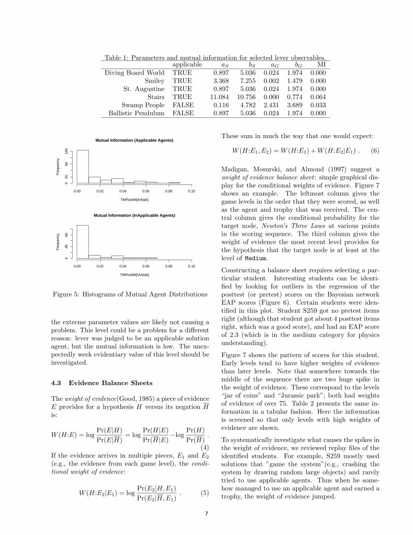
Table 1: Parameters and mutual information for selected lever observables.applicable aS bS aG bG MI

Diving Board World TRUE 0.897 5.036 0.024 1.974 0.000Smiley TRUE 3.368 7.255 0.002 1.479 0.000

St. Augustine TRUE 0.897 5.036 0.024 1.974 0.000Stairs TRUE 11.084 10.756 0.000 0.774 0.064

Swamp People FALSE 0.116 4.782 2.431 3.689 0.033Ballistic Pendulum FALSE 0.897 5.036 0.024 1.974 0.000

Mutual Information (Applicable Agents)

TMPostMI[AAtab]

Fre

quen

cy

0.00 0.02 0.04 0.06 0.08 0.10

020

6010

0

Mutual Information (InApplicable Agents)

TMPostMI[!AAtab]

Fre

quen

cy

0.00 0.02 0.04 0.06 0.08 0.10

040

80

Figure 5: Histograms of Mutual Agent Distributions

the extreme parameter values are likely not causing aproblem. This level could be a problem for a differentreason: lever was judged to be an applicable solutionagent, but the mutual information is low. The unex-pectedly week evidentiary value of this level should beinvestigated.

4.3 Evidence Balance Sheets

The weight of evidence(Good, 1985) a piece of evidenceE provides for a hypothesis H versus its negation His:

W (H:E) = logPr(E|H)

Pr(E|H)= log

Pr(H|E)

Pr(H|E)−log

Pr(H)

Pr(H).

(4)If the evidence arrives in multiple pieces, E1 and E2

(e.g., the evidence from each game level), the condi-tional weight of evidence:

W (H:E2|E1) = logPr(E2|H,E1)

Pr(E2|H,E1). (5)

These sum in much the way that one would expect:

W (H:E1, E2) = W (H:E1) +W (H:E2|E1) . (6)

Madigan, Mosurski, and Almond (1997) suggest aweight of evidence balance sheet : simple graphical dis-play for the conditional weights of evidence. Figure 7shows an example. The leftmost column gives thegame levels in the order that they were scored, as wellas the agent and trophy that was received. The cen-tral column gives the conditional probability for thetarget node, Newton’s Three Laws at various pointsin the scoring sequence. The third column gives theweight of evidence the most recent level provides forthe hypothesis that the target node is at least at thelevel of Medium.

Constructing a balance sheet requires selecting a par-ticular student. Interesting students can be identi-fied by looking for outliers in the regression of theposttest (or pretest) scores on the Bayesian networkEAP scores (Figure 6). Certain students were iden-tified in this plot. Student S259 got no pretest itemsright (although that student got about 4 posttest itemsright, which was a good score), and had an EAP scoreof 2.3 (which is in the medium category for physicsunderstanding).

Figure 7 shows the pattern of scores for this student.Early levels tend to have higher weights of evidencethan later levels. Note that somewhere towards themiddle of the sequence there are two huge spike inthe weight of evidence. These correspond to the levels“jar of coins” and “Jurassic park”; both had weightsof evidence of over 75. Table 2 presents the same in-formation in a tabular fashion. Here the informationis screened so that only levels with high weights ofevidence are shown.

To systematically investigate what causes the spikes inthe weight of evidence, we reviewed replay files of theidentified students. For example, S259 mostly usedsolutions that ”game the system”(e.g., crashing thesystem by drawing random large objects) and rarelytried to use applicable agents. Thus when he some-how managed to use an applicable agent and earned atrophy, the weight of evidence jumped.

7

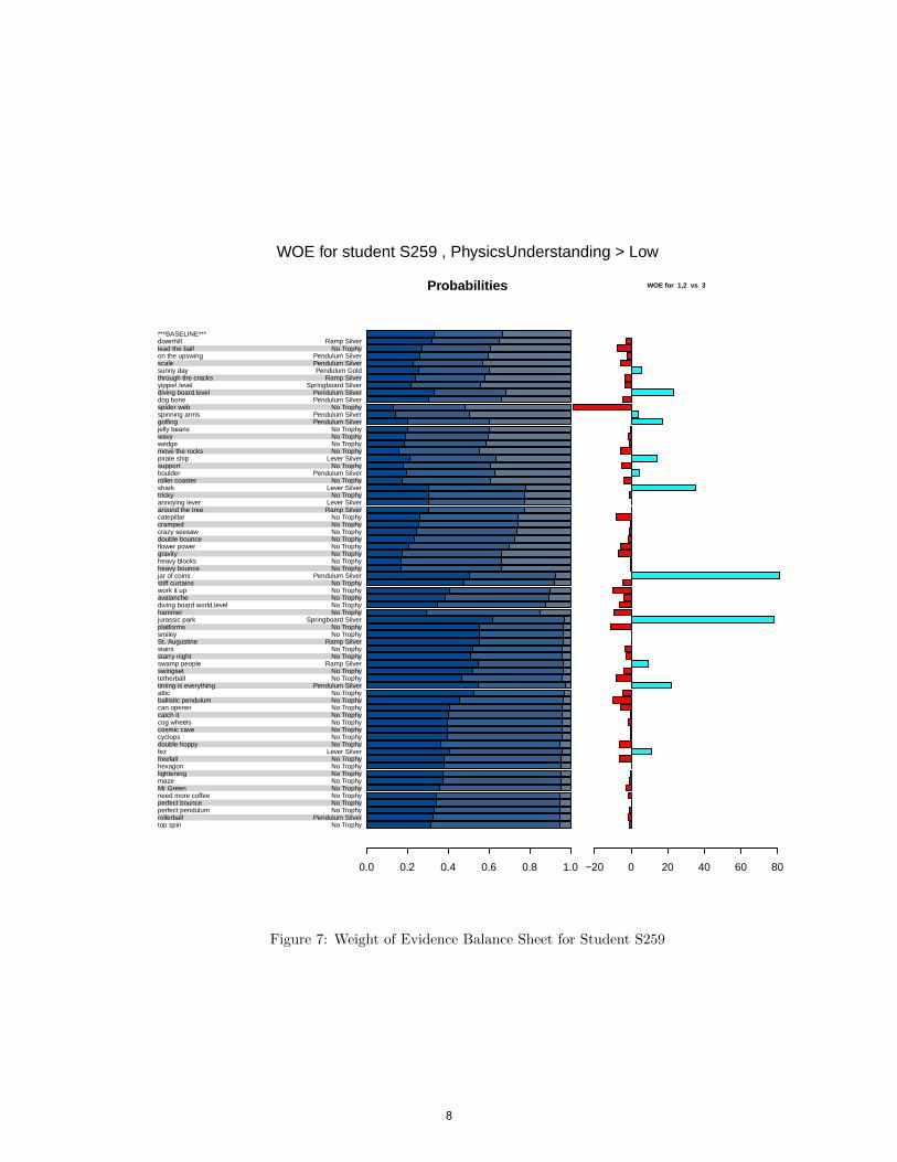
***BASELINE***downhilllead the ballon the upswingscalesunny daythrough the cracksyippie!.leveldiving board.leveldog bonespider webspinning armsgolfingjelly beanswavywedgemove the rockspirate shipsupportboulderroller coastersharktrickyannoying leveraround the treecatepillarcrampedcrazy seesawdouble bounceflower powergravityheavy blocksheavy bouncejar of coinsstiff curtainswork it upavalanchediving board world.levelhammerjurassic parkplatformssmileySt. Augustinestairsstarry nightswamp peopleswingsettetherballtiming is everythingatticballistic pendulumcan openercatch itcog wheelscosmic cavecyclopsdouble hoppyfezfreefallhexagonlighteningmazeMr Greenneed more coffeeperfect bounceperfect pendulumrollerballtop spin

Ramp SilverNo Trophy

Pendulum SilverPendulum SilverPendulum Gold

Ramp SilverSpringboard Silver

Pendulum SilverPendulum Silver

No TrophyPendulum SilverPendulum Silver

No TrophyNo TrophyNo TrophyNo Trophy

Lever SilverNo Trophy

Pendulum SilverNo Trophy

Lever SilverNo Trophy

Lever SilverRamp Silver

No TrophyNo TrophyNo TrophyNo TrophyNo TrophyNo TrophyNo TrophyNo Trophy

Pendulum SilverNo TrophyNo TrophyNo TrophyNo TrophyNo Trophy

Springboard SilverNo TrophyNo Trophy

Ramp SilverNo TrophyNo Trophy

Ramp SilverNo TrophyNo Trophy

Pendulum SilverNo TrophyNo TrophyNo TrophyNo TrophyNo TrophyNo TrophyNo TrophyNo Trophy

Lever SilverNo TrophyNo TrophyNo TrophyNo TrophyNo TrophyNo TrophyNo TrophyNo Trophy

Pendulum SilverNo Trophy

Probabilities

0.0 0.2 0.4 0.6 0.8 1.0

WOE for 1,2 vs 3

−20 0 20 40 60 80

WOE for student S259 , PhysicsUnderstanding > Low

Figure 7: Weight of Evidence Balance Sheet for Student S259

8

1.5 2.0 2.5 3.0

02

46

Bayes net (Version E) vs Posttest

Bayes Net Score

Pos

ttest

Sco

re

S259

Figure 6: Scatterplot of Postttest versus Bayes netscores.

For the case of “jar of coins”, it is one of the levels thatalready has an applicable agent built in the level as anincomplete form (i.e., pendulum for this level), and allthe player needs to do is to make the built-in agentwork by completing it (e.g., add more mass to thependulum bob). The review of his replay files revealedthat he exploited the system again for jar of coin, butthe system recognized his solution as an applicable dueto the built-in agent. This finding should lead to oneor more follow-up actions: (a) decrease discriminationfor pendulum in the CPT of jar of coins, (b) revise thelevel to make it harder to ”game” the system, and/or(c) replace the level with one that forces the player todirectly draw the agent. We chose the third option forthe next version of Newton’s Playground.

5 Lessons Learned and Future Work

The work on constructing the assessment system forNewton’s Playground is ongoing. Using these infor-mation metrics helped us identify problems in boththe code and level design. For example, one case ofunexpectedly low discrimination led to the discoveryof a bug in the code that built the observed tablesfrom the data (the labels of the High and Low cat-egories were swapped and the observation table wasbuilt upside down). Unexpected high and low infor-mation also forced the designers to take a closer lookat which agents students were actually using to solvethe problems leading to a revision in the agent tables.Finally, viewing replays led us to identify places wherethe agent identification system misidentified the agent

Table 2: Levels with high weights of evidence for Stu-dent S259

Level WOElead the ball -7.84diving board 22.92

spider web -32.59golfing 16.97

pirate ship 14.45shark 35.54

caterpillar -7.99jar of coins 80.04work it up -10.2

hammer -9.58Jurassic park 78.2

platforms -11.21swamp people 9.22

tether ball -8.32timing is everything 21.77

ballistic pendulum -9.8fez 11.38

used to solve the problem. This led to improved valuesfor the observable outcomes.

Correcting these problems lead to a definite improve-ment in the correlation between the Bayes net scoreand the pretest and posttest. With the revised net-works and evidence identification code, the correlationwith the pretest is 0.40 and with the posttest is 0.36,a definite improvement (and close to the limit of theaccuracy available given the lack of reliability of thepretest and posttest).

We have also identified some conceptual errors thatwe are still working to address. In particular, a largenumber of the students (e.g., S259) engaged in off-track “gaming” behaviors, often earning silver trophiesin the process. It is clear that the Bayesian network islacking nodes related to that kind of behavior. Also,we need a better system for detecting that kind ofbehavior. These are being implemented in Version 2.0of Newton’s Playground.

References

Almond, R. G. (2010). ‘I can name that Bayesiannetwork in two matrixes’. International Jour-nal of Approximate Reasoning , 51 , 167–178.Retrieved from http://dx.doi.org/10.1016/

j.ijar.2009.04.005

Almond, R. G., DiBello, L., Jenkins, F., Mislevy, R. J.,Senturk, D., Steinberg, L. S., et al. (2001). Mod-els for conditional probability tables in educa-tional assessment. In T. Jaakkola & T. Richard-son (Eds.), Artificial intelligence and statistics

9

2001 (p. 137-143). Morgan Kaufmann.

Almond, R. G., Kim, Y. J., Velasquez, G., & Shute,V. J. (2012, July). How task features impactevidence from assessments embedded in simula-tions and games. Lincoln, NE. (Paper presentedat the International Meeting of the PsychometricSociety (IMPS))

Almond, R. G., & Mislevy, R. J. (1999). Graphicalmodels and computerized adaptive testing. Ap-plied Psychological Measurement , 23 , 223-238.

Almond, R. G., Shute, V. J., Underwood, J. S., &Zapata-Rivera, J.-D. (2009). Bayesian networks:A teacher’s view. International Journal of Ap-proximate Reasoning , 50 , 450–460.

Almond, R. G., Steinberg, L. S., & Mislevy, R. J.(2002). Enhancing the design and delivery of as-sessment systems: A four-process architecture.Journal of Technology , Learning, and Assess-ment , 1 , (online). Retrieved from http://www

.jtla.org/

Catto, E. (2011). Box2D v2.2.0 user manual [Com-puter software manual]. Retrieved from http://

box2d.org/ (Downloaded July 25, 2012 from)

Good, I. J. (1985). Weight of evidence: A brief sur-vey. In J. Bernardo, M. DeGroot, D. Lindley, &A. Smith (Eds.), Bayesian statistics 2 (p. 249-269). North Holland.

Kolen, M. J., & Brennan, R. L. (2004/1995). Testequating, scaling, and linking: Methods andpractices (2nd ed.). Springer-Verlag.

Madigan, D., Mosurski, K., & Almond, R. G.(1997). Graphical explanation in belief net-works. Journal of Computational Graph-ics and Statistics, 6 (2), 160-181. Retrievedfrom http://www.amstat.org/publications/

jcgs/index.cfm?fuseaction=madiganjun

Mislevy, R. J., Behrens, J. T., DiCerbo, K. E., Frezzo,D. C., & West, P. (2012). Three thingsgame designers need to know about assessment.In D. Ifenthaler, D. Eseryel, & X. Ge (Eds.),Assessment in game-based learning: Founda-tions, innovations, and perspectives (pp. 59–81).Springer.

Mislevy, R. J., Steinberg, L. S., & Almond, R. G.(2003). On the structure of educational assess-ment (with discussion). Measurement: Interdis-ciplinary Research and Perspective, 1 (1), 3-62.

Muraki, E. (1992). A generalized partial credit model:Application of an em algorithm. Applied Psy-chological Measurement , 16 , 159–176.

Ploetzner, R., & VanLehn, K. (1997). The acquisi-tion of informal physics knowledge during for-mal physics training. Cognition and Instruction,15 (2), 169–205.

Shute, V. J., Hansen, E. G., & Almond, R. G.

(2008). You can’t fatten a hog by weigh-ing it - or can you? Evaluating an as-sessment for learning system called ACED.International Journal of Artificial Intelligencein Education, 18 (4), 289–316. Retrievedfrom http://www.ijaied.org/iaied/ijaied/

abstract/Vol 18/Shute08.html

Shute, V. J., & Ventura, M. (2013). Stealth assessmentin digital games. MIT series.

Shute, V. J., Ventura, M., Bauer, M. I., & Zapata-Rivera, D. (2009). Melding the power of seriousgames and embedded assessment to monitor andfoster learning: Flow and grow. In U. Ritter-feld, M. J. Cody, & P. Vorderer (Eds.), Seriousgames: Mechanisms and effects (pp. 295–321).Routledge, Taylor and Francis.

Wainer, H., Veva, J. L., Camacho, F., Reeve III,B. B., Rosa, K., Nelson, L., et al. (2001). Aug-mented scores — “borrowing strength” to com-pute scores based on a small number of items.In D. Thissen & H. Wainer (Eds.), Test scoring(pp. 343–388). Lawrence Erlbaum Associates.

Acknowledgments

Many aspects of the Newton’s Playground examplesare based on work of the Newton’s Playground team,Val Shute, P.I. In addition to the authors, the teamincludes Matthew Small, Don Franceschetti, LubinWang, and Weinan Zhao. Pete Stafford assistedwith the data analysis. Work on Newton’s Play-ground and this paper was supported by the Bill &Melinda Gates Foundation U.S. Programs Grant Num-ber #0PP1035331, Games as Learning/Assessment:Stealth Assessment. Any opinions expressed are solelythose of the authors.

10

Bayesian Supervised Dictionary learning

B. Babagholami-MohamadabadiCE Dept.

Sharif UniversityTehran, Iran

A. JourablooCE Dept.


M. ZolfaghariCE Dept.


M.T. Manzuri-ShalmaniCE Dept.


Abstract

This paper proposes a novel Bayesian methodfor the dictionary learning (DL) based clas-sification using Beta-Bernoulli process. Weutilize this non-parametric Bayesian tech-nique to learn jointly the sparse codes, thedictionary, and the classifier together. Exist-ing DL based classification approaches onlyoffer point estimation of the dictionary, thesparse codes, and the classifier and can there-fore be unreliable when the number of train-ing examples is small. This paper presentsa Bayesian framework for DL based classifi-cation that estimates a posterior distributionfor the sparse codes, the dictionary, and theclassifier from labeled training data. We alsodevelop a Variational Bayes (VB) algorithmto compute the posterior distribution of theparameters which allows the proposed modelto be applicable to large scale datasets. Ex-periments in classification demonstrate thatthe proposed framework achieves higher clas-sification accuracy than state-of-the-art DLbased classification algorithms.

1 Introduction

Sparse signal representation (Wright et al., 2010), hasrecently gained much interest in computer vision andpattern recognition. Sparse codes can efficiently rep-resent signals using linear combination of basis ele-ments which are called atoms. A collection of atomsis referred to as a dictionary. In sparse representationframework, dictionaries are usually learned from datarather than specified apriori (i.e wavelet).It has been demonstrated that using learned dictionar-ies from data usually leads to more accurate represen-tation and hence can improve performance of signalreconstruction and classification tasks (Wright et al.,

2010). Several algorithms have been proposed for thetask of dictionary learning (DL), among which the K-SVD algorithm (Aharon et al., 2006), and the Methodof Optimal Directions (MOD) (Engan et al., 1999),are the most well-known algorithms. The goal of thesemethods is to find the dictionary D = [d1,d2, ...,dK ],and the matrix of the sparse codes A = [a1, a2, ..., aN ],which minimize the following objective function

[A, D] = argminA,D‖X−DA‖2F , s.t. ‖xi‖0 ≤ T ∀i,(1)

where X = [x1, x2, ..., xN ] is the matrix of N inputsignals, K is the number of the dictionary atoms, ‖.‖Fdenotes the Frobenius norm, and ‖x‖0 denotes the l0norm which counts the number of non-zero elementsin the vector x.

2 Related Work

Classical DL methods try to find a dictionary, suchthat the reconstructed signals are fairly close to theoriginal signals, therefore they do not work well forclassification tasks. To overcome this problem, sev-eral methods have been proposed to learn a dictionarybased on the label information of the input signals.Wright (Wright et al., 2009), used training data asthe atoms of the dictionary for Face Recognition (FR)tasks. This method determines the class of each queryface image by evaluating which class leads to the min-imal reconstruction error. Although the result of thismethod on face databases are promising, it is not ap-propriate for noisy training data. Being unable to uti-lize the discriminative information of the training datais another weakness of this method.Yang (Yang et al., 2010), learned a dictionary foreach class and obtained better FR results than Wrightmethod. Yang (Yang et al., 2011), utilized Fisher Dis-criminant Analysis (FDA) to learn a sub-dictionaryfor each class in order to make the sparse coefficientsmore discriminative. Ramirez (Ramirez et al., 2010),added a structured incoherence penalty term to the

11

objective function of the class specific sub-dictionarylearning problem to make the sub-dictionaries inco-herent. Mairal (Mairal et al., 2009), introduced asupervised DL method by embedding a logistic lossfunction to learn a single dictionary and a classifiersimultaneously. Given a limited number of labeled ex-amples, most DL based classification methods sufferfrom the following problem: since these algorithmsonly provide point estimation of the dictionary, thesparse codes, and the classifier which could be sensi-tive to the choice of training examples, they tend tobe unreliable when the number of training examplesis small. In order to address the above problem, thispaper presents a Bayesian framework for superviseddictionary learning, termed Bayesian SupervisedDictionary Learning, that targets tasks where thenumber of training examples is limited. Using the fullBayesian treatment, the proposed framework for dic-tionary learning is better suited to dealing with a smallnumber of training examples than the non-Bayesianapproach.Dictionary learning based on the Bayesian non-parametric models was originally proposed by Zhou(Zhou et al., 2009), in which a prior distribution is puton the sparse codes (each sparse code is modeled as anelement-wise multiplication of a binary vector and aweight vector) which satisfies the sparsity constraint.Although the results of this method can compete withthe state of the art results in denoising, inpainting,and compressed sensing applications, it does not workwell for classification tasks due to its incapability ofutilizing the class information of the training data.To address the above problem, we extend the Bayesiannon-parametric models for classification tasks bylearning the dictionary, the sparse codes, and the clas-sifier simultaneously. The contributions of this paperare summarized as follows:

• The noise variance of the sparse codes (the spar-sity level of the sparse codes) and the dictionary islearn based on the Beta-Bernoulli process (Paisleyet al., 2009) which allows us to learn the numberof the dictionary atoms as well as the dictionaryelements.

• A logistic regression classifier (multinomial logis-tic regression (Bohning, 1992), classifier for multi-class classification) is incorporated into the prob-abilistic dictionary learning model and is learnedjointly with the dictionary and the sparse codeswhich improves the discriminative power of themodel.

• The posterior distributions of the dictionary, thesparse codes, and the classifier is efficiently com-puted via the VB algorithm which allows the

proposed model to be applicable to large-scaledatasets.

• The Bayesian prediction rule is used to classify atest instance and therefore the proposed model isless prone to overfitting, specially when the sizeof the training data is small. Precisely speaking,test instances are classified by weighted average ofthe parameters (the dictionary, the sparse codes ofthe test instances , and the classifier), weighted bythe posterior probability of each parameter valuegiven the training data.

• Using the Beta-Bernoulli process model, manycomponents of the learned sparse codes are ex-actly zero, which is different from the widely usedLaplace prior, in which many coefficients of thesparse codes are small but not exactly zero.

The remainder of this paper is organized as follows:Section 3 briefly reviews the Beta-Bernoulli process.The proposed method is introduced in Section 4. Ex-perimental results are presented in Section 5. We con-clude and discuss future work in Section 6.

3 Beta-Bernoulli Process

The Beta process B ∼ BP (c,B0) is an example of aLevy process which was originally proposed by Hjortfor survival analysis (Hjort, 1990), and can be definedas a distribution on positive random measures over ameasurable space (Ω,F).B0 is the base measure defined over Ω and c(ω) is apositive function over Ω which is assumed constant forsimplicity. The Levy measure of B ∼ BP (c,B0) isdefined as

ν(dπ, dω) = cπ−1(1− π)c−1dπB0(dω). (2)

In order to draw samples from B ∼ BP (c,B0), King-man (Kingman, 1993), proposed a procedure based onthe Poisson process which goes as follows.First, a non-homogeneous Poisson process is defined onΩ ×R+ with intensity function ν. Then, Poisson(λ)number of points (πk, ωk) ∈ [0, 1]× Ω are drawn fromthe Poisson process (λ =

∫[0,1]

∫Ων(dω, dπ) =∞). Fi-

nally, a draw from B ∼ BP (c,B0) is constructed as

Bω =∞∑k=1

πkδωk, (3)

where δωkis a unit point measure at ωk (δωk

equalsone if ω = ωk and is zero otherwise) . It can be seenfrom equation 3, that Bω is a discrete measure (withprobability one), for which Bω(A) =

∑k:ωk∈A πk, for

any set A ⊂ F .

12

If we define Z = Be(B) as a Bernoulli process with Bωdefined as 3, a sample from this process can be drawnas

Z =∞∑k=1

zkδωk, (4)

where zk is generated by

zk ∼ Bernoulli(πk). (5)

If we draw N samples (Z1, ..., ZN ) from the Bernoulliprocess Be(B) and arrange them in matrix form, Z =[Z1, ..., ZN ], then the combination of the Beta processand the Bernoulli process can be considered as a priorover infinite binary matrices, with each column Zi inthe matrix Z corresponding to a location, δωi

. Bymarginalizing out the measure B, the joint probabilitydistribution P (Z1, ..., ZN ) corresponds to the IndianBuffet Process (Thibaux et al., 2007).

4 Proposed Method

All previous classification based sparse coding anddictionary learning methods have three shortcomings.First, the noise variance or the sparsity level of thesparse codes must be specified apriori in order to definethe stopping criteria for estimating the sparse codes.Second, the number of the dictionary atoms must beset in advance (or determined via the cross-validationtechnique). Third, a point estimate of the dictionaryand the sparse codes are used to predict the class la-bel of the test data points which can result in overfit-ting. To circumvent these shortcomings, we proposea Bayesian probabilistic model in terms of the Beta-Bernoulli process which can infer both the dictionarysize and the noise variance of the sparse codes fromdata. Furthermore, our approach integrates a logis-tic regression classifier (multinomial logistic regressionclassifier for multiclass classification) into the proposedprobabilistic model to learn the dictionary and theclassifier simultaneously while most of the algorithmslearn the dictionary and the classifier separately.

4.1 Problem Formulation

Consider we are given a training set of N labeled sig-nals X = [x1,x2, ...,xN ] ∈ RM×N , each of them maybelong to any of the c different classes. We first con-sider the case of c = 2 classes and later discuss themulticlass extension. Each signal is associated with alabel (yi ∈ −1, 1, i = 1, ..., N). We model each signalxi, as a sparse combination of atoms of a dictionaryD ∈ RM×K , with an additive noise εi. The Matrixform of the model can be formulated as

X = DA+ E, (6)

where XM×N is the set of the input signals, AK×Nis the set of the K dimensional sparse codes, andE ∼ N (0, γ−1

x IM ) is the zero-mean Gaussian noisewith precision value γx (IM is an M ×M Identity ma-trix). Following (Zhou, 2009), we model the matrixof the sparse codes (A) as an element-wise multiplica-tion of a binary matrix (Z) and a weight matrix (S).Hence, the model of equation 6 can be reformulated as

X = D(Z S) + E, (7)

where is the element-wise multiplication operator.We put a prior distribution on the binary matrix Z us-ing the extension of the Beta-Bernoulli process whichtakes two scalar parameters a and b and was origi-nally proposed by (Paisley, 2009). A sample from theextended Beta process B ∼ BP (a, b, B0) with basemeasure B0 may be represented as

Bω =K∑k=1

πkδωk, (8)

where,

πk ∼ Beta(a/K, b(K − 1)/K), ωk ∼ B0. (9)

This sample will be a valid sample from the extendedBeta process, if K → ∞. Bω can be considered asa vector of K probabilities that each probability πkcorresponds to the atom ωk. In our framework, weconsider each atom ωk as the k-th atom of the dictio-nary (dk) and we set the base measure B0 to a multi-variate zero-mean Gaussian distribution N (0, γ−1

d IK)(with precision value γd) for simplicity. So, by lettingK → ∞, the number of the dictionary atoms can belearned from the training data. To model the weights(si)

Ni=1, we use a zero-mean Gaussian distribution with

precision value γs.In order to make the dictionary discriminative for theclassification purpose, we incorporate a logistic regres-sion classifier to our probabilistic model. More pre-cisely, if αt = zt st be the sparse code of a test in-stance xt, the probability of yt = +1 can be computedusing the logistic sigmoid acting on a linear functionof αt so that

P (yt = +1 | zt, st,w, w0) = σ(wT (zt st) + w0),(10)

where σ(x) is the logistic function which is defined as

σ(x) =1

1 + e−x. (11)

As the probability of the two classes must sum to 1,we have P (yt = −1 | zt, st,w, w0) = 1 − P (yt = +1 |zt, st,w, w0). Since the logistic function has the prop-erty that σ(−x) = 1 − σ(x), we can write the classconditional probability more concisely as

P (yt | zt, st,w, w0) = σ(yt[w

T (zt st) + w0]), (12)

13

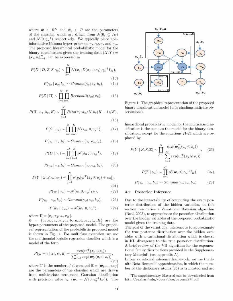
where w ∈ RK and w0 ∈ R are the parametersof the classifier which are drawn from N (0, γ−1

w IK)and N (0, γ−1

w ) respectively. We typically place non-informative Gamma hyper-priors on γx, γd, γs and γw.The proposed hierarchical probabilistic model for thebinary classification given the training data (X,Y ) =(xi, yi)

Ni=1, can be expressed as

P (X | D,Z, S, γx) ∼N∏j=1

N (xj ;D(zj sj), γ−1x IM ),

(13)

P (γx | ax, bx) ∼ Gamma(γx; ax, bx), (14)

P (Z | Π) ∼N∏i=1

K∏k=1

Bernoulli(zki;πk), (15)

P (Π | aπ, bπ,K) ∼K∏k=1

Beta(πk; aπ/K, bπ(K − 1)/K),

(16)

P (S | γs) ∼N∏i=1

K∏k=1

N (ski; 0, γ−1s ), (17)

P (γs | as, bs) ∼ Gamma(γs; as, bs), (18)

P (D | γd) ∼M∏i=1

K∏k=1

N (dik; 0, γ−1d ), (19)

P (γd | ad, bd) ∼ Gamma(γd; ad, bd), (20)

P (Y | Z, S,w, w0) ∼N∏j=1

σ(yj [wT (zj sj) + w0]),

(21)

P (w | γw) ∼ N (w; 0, γ−1w IK), (22)

P (γw | aw, bw) ∼ Gamma(γw; aw, bw), (23)

P (w0 | γw0) ∼ N (w0; 0, γ−1w ), (24)

where Π = [π1, π2, ..., πK ].Φ = aπ, bπ, ax, bx, ad, bd, as, bs, aw, bw,K are thehyper-parameters of the proposed model. The graphi-cal representation of the probabilistic proposed modelis shown in Fig. 1. For multiclass extension, we usethe multinomial logistic regression classifier which is amodel of the form

P (yt = c | zt, st,Ξ) =exp(wT

c (zt st))∑Cc′=1 exp(w

Tc′(zt st))

,

(25)where C is the number of classes and Ξ = [w1, ...,wC ]are the parameters of the classifier which are drawnfrom multivariate zero-mean Gaussian distributionwith precision value γw (wc ∼ N (0, γ−1

w IK)). The

Figure 1: The graphical representation of the proposedbinary classification model (blue shadings indicate ob-servations).

hierarchical probabilistic model for the multiclass clas-sification is the same as the model for the binary clas-sification, except for the equations 21-24 which are re-placed by

P (Y | Z, S,Ξ) ∼N∏j=1

exp(wTyj (zj sj)

)C∑c=1

exp(wTc (zj sj))

, (26)

P (Ξ | γw) ∼C∏c=1

N (wc; 0, γ−1w IK), (27)

P (γw | aw, bw) ∼ Gamma(γw; aw, bw). (28)

4.2 Posterior Inference

Due to the intractability of computing the exact pos-terior distribution of the hidden variables, in thissection, we derive a Variational Bayesian algorithm(Beal, 2003), to approximate the posterior distributionover the hidden variables of the proposed probabilisticmodel given the training data.The goal of the variational inference is to approximatethe true posterior distribution over the hidden vari-ables with a variational distribution which is closestin KL divergence to the true posterior distribution.A brief review of the VB algorithm for the exponen-tional family distributions provided in the Supplemen-tary Material1 (see appendix A).In our variational inference framework, we use the fi-nite Beta-Bernoulli approximation, in which the num-ber of the dictionary atoms (K) is truncated and set

1The supplementary Material can be downloaded fromhttp://ce.sharif.edu/∼jourabloo/papers/SM.pdf

14

http://ce.sharif.edu/~jourabloo/papers/SM.pdf

to a finite but large number. If K is large enough, theanalyzed data using this number of dictionary atoms,will reveal less than K components.In the following two sections, we derive the variationalupdate equations for the binary and the multiclassclassification models.

4.2.1 Variational Inference For the BinaryClassification

In the proposed binary classification model, the hiddenvariables are

W =

Π = [π1, π2, ..., πK ], Z = [z1, z2, ...,zN ],

S = [s1, s2, ..., sN ], D = [d1,d2, ...,dK ],w, w0,

γs, γw, γx, γd

.

We use a fully factorized variational distribution whichis as follows

q(Π, Z, S,D,w, w0, γs, γw, γx, γd) =

K∏k=1

M∏i=1

qπk(πk)qdik(dik)

N∏j=1

K∏k=1

qzkj(zkj)qskj

(skj)×

qw(w)qw0(w0)qγs(γs)qγw(γw)qγx(γx)qγd(γd).

It’s worth noting that instead of using the parame-terized variational distribution, we use the factorizedform of the variational inference which is called MeanField method (Beal, 2003). More precisely, we derivethe form of the distribution q(x) by optimizing the KLdivergence over all possible distributions.Based on the graphical model of Fig. 1, the joint prob-ability distribution of the observations (training data)and the hidden variables can be expressed as

P (X,Y,W | Φ) =

N∏j=1

(P (xj | zj , sj , D, γx)P (yj | zj , sj ,w, w0)

)×

K∏k=1

(P (πk | aπ, bπ)

N∏j=1

P (zkj | πk)P (skj | γs)×

M∏i=1

P (dik | γd))P (w | γw)P (w0 | γw)P (γs | as, bs)×

P (γx | ax, bx)P (γw | aw, bw)P (γd | ad, bd). (29)

In the binary classification model, all of the distribu-tions are in the conjugate exponential family exceptfor the logistic function. Due to the non-conjugacybetween the logistic function and Guassian distribu-tion, deriving the VB update equations in closed-formis intractable. To overcome this problem, we use the

local lower bound to the sigmoid function proposed by(Jaakkola et al., 2000), which states that for any x ∈ Rand ξ ∈ [0,+∞]

1

1 + exp(−x)≥ σ(ξ)exp

((x− ξ)/2− λ(ξ)(x2 − ξ2)

),

(30)where,

λ(ξ) =−1

2ξ

( 1

1 + exp(−ξ)− 1

2

). (31)

ξ is the free variational parameter which is optimizedto get the tightest possible bound. Hence, we replaceeach sigmoid factor in the joint probability distribu-tion (equation 29) with the above lower bound (equa-tion 30), then we use the EM algorithm to optimize thefactorized variational distribution and the free param-eters (ξ = ξ1, ξ2, ..., ξN) which computes the varia-tional posterior distribution in the E-step and maxi-mizes the free parameters in the M-step. All updateequations are available in the Supplementary Material(see appendix B).

4.2.2 Variational Inference For theMulticlass Classification

In the proposed multiclass classification model, be-cause of non-conjugacy between the multinomial lo-gistic regression function (equation 25) and the Gaus-sian distribution, deriving the VB update equationsin closed-form is intractable. To tackle this non-conjugacy problem, we utilize the following simple in-equality which was originally proposed by (Bouchard,2007), which states that for every βcCc=1 ∈ R andα ∈ R,

log( C∑c=1

eβc)≤ α+

C∑c=1

log(1 + eβc−α

). (32)

If we replace x with α − βc in the equation 30, andtake the logarithm of the both sides of that equation,we have

log(1 + eβc−α) ≤ λ(ξ)((βc − α)2 − ξ2

)−

log σ(ξ) +((βc − α) + ξ

)/2. (33)

Then, by replacing each term in the summation ofthe right hand side of the equation 32 with the up-per bound of the equation 33, we have

log( C∑c=1

eβc)≤ α+

C∑c=1

log(1 + eβc−α

)≤

C∑c=1

(λ(ξc)

((βc − α)2 − ξ2

c

)− log σ(ξc)

)+

α+1

2

C∑c=1

(βc − α+ ξc). (34)

15

We utilize the above inequality for approximating thedenominator of the right hand side of the equation 26.So, for the proposed multiclass classification model,the free parameters are

αiNi=1, ξij

N ,Ci=1,j=1

.

We derive an EM algorithm that computes the vari-ational posterior distribution in the E-step and maxi-mizes the free parameters in the M-step. Details of theupdate equations are available in the SupplementaryMaterial (see appendix C).

4.3 Class Label Prediction

After computing the posterior distribution, in or-der to determine the target class-label yt of a giventest instance xt, we first compute the predictive dis-tribution of the target class label given the testinstance by integrating out the hidden variables(D, γx, zt, st,w, w0 for binary classification model,and D, γx, zt, st, [wc]

Cc=1 for multiclass classification

model), then we pick the label with the maximumprobability value. For binary classification, this pro-cedure can be formulated as

yt = argmaxyt∈−1,1P (yt | xt, T ), (35)

where T = (xj , yj)Nj=1 is the training data. P (yt |

xt, T ) can be computed as

P (yt | xt, T ) =∑zt

∫∫∫P (yt, st, zt,w, w0 | xt, T )dst dw dw0

=∑zt

∫∫∫P (yt | st, zt,w, w0, xt, T )×

P (st, zt,w, w0 | xt, T )dst dw dw0

=∑zt

∫∫∫σ(yt[w

T (st zt) + w0])P (st, zt | xt, T )×

P (w | T )P (w0 | T )dst dw dw0

≈∑zt

∫∫∫σ(yt[w

T (st zt) + w0])P (st, zt | xt, T )×

q∗(w)q∗(w0)dst dw dw0, (36)

where we replaced P (w | T ) and P (w0 | T ) with theapproximate posterior distributions q∗(w) and q∗(w0)respectively.Since the above expression cannot be computed inclosed form, we resort to Monte Carlo sampling to ap-proximate that expression. In other words, we approx-imate the distribution P (st, zt | xt, X, Y )q∗(w)q∗(w0)with l samples, then we compute P (yt | xt, T ) as

P (yt | xt, T ) ≈ 1

l

∑l

σ(yt[(wl)T (sltzlt) +wl0]), (37)

where rl is the l-th sample of the hidden variable r.Since the approximate posterior distributions q∗(w)

Figure 2: The graphical model of the Gibbs samplingmethod.

and q∗(w0) are Gaussian (see the appendix B of theSupplementary Material), sampling from these distri-butions is straightforward. P (st, zt | xt, T ) can becomputed as

P (st, zt | xt, T ) =P (xt | st, zt, T )P (st, zt | T )

P (xt | T ),

(38)

which cannot be directly sampled from. Therefore,to sample from P (st, zt | xt, T ), we sample fromP (st, zt, D,Π, γs, γx | xt, T ) based on the Gibbs sam-pling method (Robert et al., 2004), then simply ig-nore the values for D,Π, γs, γx in each sample. Thegraphical model in Fig. 2 shows all the relevant pa-rameters and conditional dependence relationships, bywhich the Gibbs sampling equations are derived. Thedetailes of the Gibbs sampling equations are avalablein the Supplementary Material (see appendix D). Itshould be noted that the parameters of the variablesin Fig. 2 are the updated parameters of the variationalposterior distribution which were computed using VBalgorithm (see appendix B of the Supplementary Ma-terial). For multiclass extension, the posterior distri-bution over the class label of a test instance xt can beapproximated as

P (yt = c | xt, T ) ≈ 1

l

∑l

exp((wl

c)T (zlt slt)

)∑Cc′=1 exp((w

lc′)

T (zlt slt)),

(39)where wl

cCc=1 are the l-th samples of the approximateposterior distributions q∗(wc)Cc=1, and (zlt, s

lt) is the

l-th sample of the posterior distribution P (st, zt |xt, T ).Sampling from q∗(wc)Cc=1 is straightforward. Sam-pling from the distribution P (st, zt | xt, T ) for multi-class classification model is the same as sampling fromthat distribution for the binary classification model(see appendix D).

16

5 Experimental Results

In this section, we verify the performance of the pro-posed method on various applications such as digitrecognition, face recognition, and spoken letter recog-nition. For applications which include more than twoclasses, we use one versus all binary classification (oneclassifier for each class) based on the proposed binaryclassification model (PMb) as well as the proposedmulticlass classification model (PMm).All of the experimental results are averaged over sev-eral runs of randomly generated splits of the data.Moreover, in all experiments, all Gamma priors areset as Gamma (10−6, 10−6) to make the prior distri-butions uninformative. The parameters aπ, bπ of theBeta distribution are set with aπ = K and bπ = K/2(many other settings of aπ and bπ yield similar results).For the Gibbs sampling inference, we discard the ini-tial 500 samples (burn-in period), and collect the next1000 samples to present the posterior distribution overthe sparse code of a test instance.

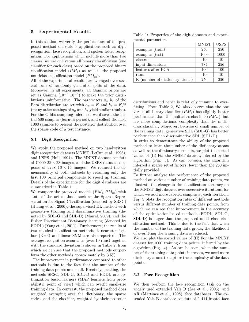
5.1 Digit Recognition

We apply the proposed method on two handwrittendigit recognition datasets MNIST (LeCun et al., 1998),and USPS (Hull, 1994). The MNIST dataset consistsof 70000 28 × 28 images, and the USPS dataset com-poses of 9298 16 × 16 images. We reduced the di-mensionality of both datasets by retaining only thefirst 100 principal components to speed up training.Details of the experiments for the digit databases aresummarized in Table 1.We compare the proposed models (PMb, PMm) withstate of the art methods such as the Sparse Repre-sentation for Signal Classification (denoted by SRSC)(Huang et al., 2006), the supervised DL method withgenerative training and discriminative training (de-noted by SDL-G and SDL-D) (Mairal, 2009), and theFisher Discriminant Dictionary learning (denoted byFDDL) (Yang et al., 2011). Furthermore, the results oftwo classical classification methods, K-nearest neigh-bor (K=3) and linear SVM are also reported. Theaverage recognition accuracies (over 10 runs) togetherwith the standard deviation is shown in Table 2, fromwhich we can see that the proposed methods outper-form the other methods approximately by 3.5%.The improvement in performance compared to other

methods is due to the fact that the number of thetraining data points are small. Precisely speaking, themethods SRSC, SDL-G, SDL-D and FDDL are op-timization based learners (MAP learners from prob-abilistic point of view) which can overfit small-sizetraining data. In contrast, the proposed method doesweighted averaging over the dictionary, the sparsecodes, and the classifier, weighted by their posterior

Table 1: Properties of the digit datasets and experi-mental parameters

MNIST USPSexamples (train) 250 250examples (test) 1000 1000classes 10 10input dimensions 784 256features after PCA 100 100runs 10 10K (number of dictionary atoms) 250 250

distributions and hence is relatively immune to over-fitting. From Table 2, We also observe that the oneversus all binary classifier (PMb) has slightly betterperformance than the multiclass classifier (PMm), buthas more computational complexity than the multi-class classifier. Moreover, because of small number ofthe training data, generative SDL (SDL-G) has betterperformance than discriminative SDL (SDL-D).In order to demonstrate the ability of the proposedmethod to learn the number of the dictionary atomsas well as the dictionary elements, we plot the sortedvalues of 〈Π〉 For the MNIST dataset, inferred by thealgorithm (Fig. 3). As can be seen, the algorithminferred a sparse set of factors, fewer than the 250 ini-tially provided.To further analyze the performance of the proposedmethod on various number of training data points, weillustrate the change in the classification accuracy onthe MNIST digit dataset over successive iterations, forwhich we add more labeled samples at each iteration.Fig. 5 plots the recognition rates of different methodsversus different number of training data points, fromwhich we can see that improvement in the accuracyof the optimization based methods (FDDL, SDL-G,SDL-D) is larger than the proposed multi class clas-sification method. This is due to the fact that whenthe number of the training data grows, the likelihoodof overfitting the training data is reduced.We also plot the sorted values of 〈Π〉 For the MNISTdataset for 1000 training data points, inferred by thealgorithm (Fig. 4). As can be seen, when the num-ber of the training data points increases, we need moredictionary atoms to capture the complexity of the datapoints.

5.2 Face Recognition

We then perform the face recognition task on thewidely used extended Yale B (Lee et al., 2005), andAR (Martinez et al., 1998), face databases. The ex-tended Yale B database consists of 2, 414 frontal-face

17

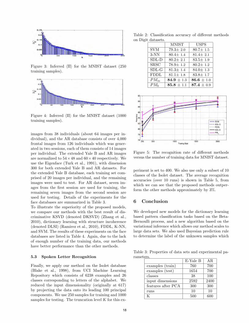
Figure 3: Inferred 〈Π〉 for the MNIST dataset (250training samples).

Figure 4: Inferred 〈Π〉 for the MNIST dataset (1000training samples).

images from 38 individuals (about 64 images per in-dividual), and the AR database consists of over 4,000frontal images from 126 individuals which was gener-ated in two sessions, each of them consists of 14 imagesper individual. The extended Yale B and AR imagesare normalized to 54×48 and 60×40 respectively. Weuse the Eigenface (Turk et al., 1991), with dimension300 for both extended Yale B and AR datasets. Forthe extended Yale B database, each training set com-prised of 20 images per individual, and the remainingimages were used to test. For AR dataset, seven im-ages from the first session are used for training, theremaining seven images from the second session areused for testing. Details of the experiments for theface databases are summarized in Table 3.To illustrate the superiority of the proposed models,we compare our methods with the best result of dis-criminative KSVD (denoted DKSVD) (Zhang et al.,2010), dictionary learning with structure incoherence(denoted DLSI) (Ramirez et al., 2010), FDDL, K-NN,and SVM. The results of these experiments on the facedatabases are listed in Table 4. Again, due to the lackof enough number of the training data, our methodshave better performance than the other methods.

5.3 Spoken Letter Recognition

Finally, we apply our method on the Isolet database(Blake et al., 1998), from UCI Machine LearningRepository which consists of 6238 examples and 26classes corresponding to letters of the alphabet. Wereduced the input dimensionality (originally at 617)by projecting the data onto its leading 100 principalcomponents. We use 250 samples for training and 1000samples for testing. The truncation level K for this ex-

Table 2: Classification accuracy of different methodson Digit datasets.

MNIST USPSSVM 79.3± 2.0 80.7± 1.5

3-NN 80.4± 1.4 81.4± 2.1

SDL-D 80.2± 2.1 83.5± 1.9

SRSC 78.9± 1.2 80.2± 1.2

SDL-G 81.3± 1.4 84.0± 1.3

FDDL 81.1± 1.8 83.8± 1.7

PMm 84.9 ± 1.3 86.6 ± 1.0

PMb 85.8 ± 1.1 87.4 ± 0.9

Figure 5: The recognition rate of different methodsversus the number of training data for MNIST dataset.

periment is set to 400. We also use only a subset of 10classes of the Isolet dataset. The average recognitionaccuracies (over 10 runs) is shown in Table 5, fromwhich we can see that the proposed methods outper-form the other methods approximately by 3%.

6 Conclusion

We developed new models for the dictionary learningbased pattern classification tasks based on the Beta-Bernoulli process, and a new algorithm based on thevariational inference which allows our method scales tolarge data sets. We also used Bayesian prediction ruleto determine the label of the unknown samples which

Table 3: Properties of data sets and experimental pa-rameters.

E-Yale B ARexamples (train) 760 700examples (test) 1654 700classes 38 100input dimensions 2592 2400features after PCA 300 300runs 10 10K 500 600

18

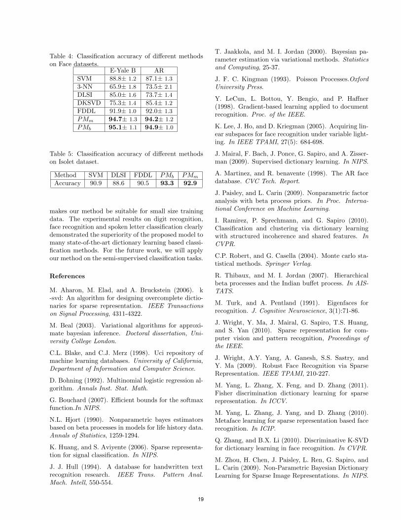
Table 4: Classification accuracy of different methodson Face datasets.

E-Yale B ARSVM 88.8± 1.2 87.1± 1.3

3-NN 65.9± 1.8 73.5± 2.1

DLSI 85.0± 1.6 73.7± 1.4

DKSVD 75.3± 1.4 85.4± 1.2

FDDL 91.9± 1.0 92.0± 1.3

PMm 94.7± 1.3 94.2± 1.2

PMb 95.1± 1.1 94.9± 1.0

Table 5: Classification accuracy of different methodson Isolet dataset.

Method SVM DLSI FDDL PMb PMm

Accuracy 90.9 88.6 90.5 93.3 92.9

makes our method be suitable for small size trainingdata. The experimental results on digit recognition,face recognition and spoken letter classification clearlydemonstrated the superiority of the proposed model tomany state-of-the-art dictionary learning based classi-fication methods. For the future work, we will applyour method on the semi-supervised classification tasks.

References

M. Aharon, M. Elad, and A. Bruckstein (2006). k-svd: An algorithm for designing overcomplete dictio-naries for sparse representation. IEEE Transactionson Signal Processing, 4311-4322.

M. Beal (2003). Variational algorithms for approxi-mate bayesian inference. Doctoral dissertation, Uni-versity College London.

C.L. Blake, and C.J. Merz (1998). Uci repository ofmachine learning databases. University of California,Department of Information and Computer Science.

D. Bohning (1992). Multinomial logistic regression al-gorithm. Annals Inst. Stat. Math.

G. Bouchard (2007). Efficient bounds for the softmaxfunction.In NIPS.

N.L. Hjort (1990). Nonparametric bayes estimatorsbased on beta processes in models for life history data.Annals of Statistics, 1259-1294.

K. Huang, and S. Aviyente (2006). Sparse representa-tion for signal classification. In NIPS.

J. J. Hull (1994). A database for handwritten textrecognition research. IEEE Trans. Pattern Anal.Mach. Intell, 550-554.

T. Jaakkola, and M. I. Jordan (2000). Bayesian pa-rameter estimation via variational methods. Statisticsand Computing, 25-37.

J. F. C. Kingman (1993). Poisson Processes.OxfordUniversity Press.

Y. LeCun, L. Bottou, Y. Bengio, and P. Haffner(1998). Gradient-based learning applied to documentrecognition. Proc. of the IEEE.

K. Lee, J. Ho, and D. Kriegman (2005). Acquiring lin-ear subspaces for face recognition under variable light-ing. In IEEE TPAMI, 27(5): 684-698.

J. Mairal, F. Bach, J. Ponce, G. Sapiro, and A. Zisser-man (2009). Supervised dictionary learning. In NIPS.

A. Martinez, and R. benavente (1998). The AR facedatabase. CVC Tech. Report.

J. Paisley, and L. Carin (2009). Nonparametric factoranalysis with beta process priors. In Proc. Interna-tional Conference on Machine Learning.

I. Ramirez, P. Sprechmann, and G. Sapiro (2010).Classification and clustering via dictionary learningwith structured incoherence and shared features. InCVPR.

C.P. Robert, and G. Casella (2004). Monte carlo sta-tistical methods. Springer Verlag.

R. Thibaux, and M. I. Jordan (2007). Hierarchicalbeta processes and the Indian buffet process. In AIS-TATS.

M. Turk, and A. Pentland (1991). Eigenfaces forrecognition. J. Cognitive Neuroscience, 3(1):71-86.

J. Wright, Y. Ma, J. Mairal, G. Sapiro, T.S. Huang,and S. Yan (2010). Sparse representation for com-puter vision and pattern recognition, Proceedings ofthe IEEE.

J. Wright, A.Y. Yang, A. Ganesh, S.S. Sastry, andY. Ma (2009). Robust Face Recognition via SparseRepresentation. IEEE TPAMI, 210-227.

M. Yang, L. Zhang, X. Feng, and D. Zhang (2011).Fisher discrimination dictionary learning for sparserepresentation. In ICCV.

M. Yang, L. Zhang, J. Yang, and D. Zhang (2010).Metaface learning for sparse representation based facerecognition. In ICIP.

Q. Zhang, and B.X. Li (2010). Discriminative K-SVDfor dictionary learning in face recognition. In CVPR.

M. Zhou, H. Chen, J. Paisley, L. Ren, G. Sapiro, andL. Carin (2009). Non-Parametric Bayesian DictionaryLearning for Sparse Image Representations. In NIPS.

19

Identifying Learning Trajectories in an Educational Video Game

Deirdre Kerr

UCLA/CRESST Peter V. Ueberroth Building (PVUB)

10945 Le Conte Ave., Suite 1400 Los Angeles, CA 90095-7150

[email protected]

Gregory K.W.K. Chung

UCLA/CRESST Peter V. Ueberroth Building (PVUB)

10945 Le Conte Ave., Suite 1355 Los Angeles, CA 90095-7150

[email protected]

Abstract

Educational video games and simulations hold great potential as measurement tools to assess student levels of understanding, identify effective instructional techniques, and pinpoint moments of learning because they record all actions taken in the course of solving each problem rather than just the answers given. However, extracting meaningful information from the log data produced by educational video games and simulations is notoriously difficult. We extract meaningful information from the log data by first utilizing a logging technique that results in a far more easily analyzed dataset. We then identify different learning trajectories from the log data, determine the varying effects of the trajectories on learning, and outline an approach to automating the process.

1. INTRODUCTION

Computer games and simulations hold great potential as measurement tools because they can measure knowledge that is difficult to assess using paper-and-pencil tests or hands-on tasks (Quellmalz & Pellegrino, 2009). These measures can then be used to support diagnostic claims about students’ learning processes (Leighton & Gierl, 2007), provide detailed measures of the extent to which players have mastered specific learning goals (National Science and Technology Council, 2011), and generate information that can be used to improve classroom instruction (Merceron & Yacef, 2004).

Log files from games can store complete student answers to the problems (Merceron & Yacef, 2004), allowing the

researcher to record unobtrusively (Kim, Gunn, Schuh, Phillips, Pagulayan, & Wixon, 2008; Mostow, Beck, Cuneao, Gouvea, Heiner, & Juarez, 2011) the exact learning behavior of students (Romero & Ventura, 2007) that is not always captured in written or verbal explanations of their thought processes (Bejar, 1984).

Though log data is more comprehensive and more detailed than most other forms of assessment data, analyzing such data presents a number of problems because the log files typically include thousands of pieces of information for each student (Romero, Gonzalez, Ventura, del Jesus, & Herrera, 2009) with no known theory to help identify which information is salient (National Research Council, 2011). Additionally, the specific information stored in the log files is not always easy to interpret (Romero & Ventura, 2007) as the responses of individual students are highly context dependent (Rupp, Gusta, Mislevy, & Shaffer, 2010) and it can be very difficult to picture how student knowledge, learning, or misconceptions manifest themselves at the level of a specific action taken by the student in the course of the game. Due to these difficulties, there is currently no systematic approach to extracting relevant data from log files (Muehlenbrock, 2005). The interpretation of the rich stream of complex data that results from the tracking of in-game actions is one of the most serious bottlenecks facing researchers examining educational video games and simulations today (Mislevy, Almond, & Lukas, 2004).

1.1 RELATED WORK

Due to the difficulty involved in analyzing log data of students’ in-game performance, educational researchers occasionally analyze student in-game performance by hand, despite the size of the data. Trained human raters have been used to extract purposeful sets of actions from game logs (Avouris, Komis, Fiotakis, Margaritis, &

20

Voyiatzaki, 2005) and logs of eye-tracking data (Conati & Merten, 2007). One study hand-identified student errors in log files from an introductory programming environ-ment (Vee, Meyer, & Mannock, 2006) and another examined behavior patterns in an exploratory learning environment by hand to categorize students into learning types (Amershi & Conati, 2011). Another had the teacher play the role of a game character to score student responses and provide live feedback to the students (Hickey, Ingram-Goble, & Jameson, 2009).

Other studies avoided hand-coding log data by using easily extracted in-game measures such as percent completion or time spent on task to measure performance. The number of activities completed in the online learning environments Moodle (Romero, Gonzalez, Ventura, del Jesus, & Herrera, 2009) and ActiveMath (Scheuer, Muhlenbrock, & Melis, 2007) have been used to predict student grades. The time spent in each activity in an online learning environment has been used to detect unusual learning behavior (Ueno & Nagaoka, 2002). Combinations of the total time spent in the online environment and the number of activities successfully completed have been used to predict student success (Muhlenbrock, 2005) and report student progress (Rahkila & Karjalainen, 1999).

1.2 OUR CONTRIBUTION

In this study, we identify learning trajectories from information stored in log data generated by an educational video game. We do this by extracting the number of attempts required to solve each level (rather than the time spent or the number of levels completed) and then hand clustering the individual learning trajectories that result from plotting the attempts over time. We show that this process results in the identification of substantively different types of learning trajectories that differ on a variety of measures. We also discuss the benefits of our logging, preprocessing, and exploratory analysis techniques in regards to ease of interpretation and potential use in data mining techniques.

1.3 SAMPLE

This study uses data from 859 students who played an educational video game about identifying fractions called Save Patch in their classrooms for four days as part of a larger study. These students were given a paper-and-pencil pretest to measure their prior knowledge of fractions. After they played the game, students were given both an immediate posttest and a delayed posttest. The immediate posttest was computerized and was given on the last day of game play. The delayed posttest was a paper-and-pencil test that was given a few weeks later. All three tests consisted of both a set of content items and a set of survey items. In addition, the game generated log data consisting of each action taken by each student in the course of game play. The resulting dataset consisted of 1,288,103 total actions, 17,685 of which were unique.

2. DATA PREPARATION

The Data Preprocessing and Intelligent Data Analysis article (Famili, Shen, Weber, & Simoudis, 1997) lists eleven problems with real-world data that should be addressed in preprocessing. Our data comes from a single source, so we do not have to worry about merging data from multiple sources or combining incompatible data. The nine remaining problems and how they are applicable to our data are shown in Table 1.

Table 1: Potential Problems with Save Patch Data

PROBLEM DESCRIPTION

Corruption and noise

Interruptions during data recording can lead to missing actions

Feature extraction

Important events must be identified from sets of individual actions

Irrelevant data

Not all actions taken in the game are meaningful

Volume of data

Hundreds or thousands of actions are recorded for each student

Missing attributes

Logs can fail to capture all relevant attributes

Missing attribute values

Logs can fail to record all values for all captured attributes

Numeric and symbolic data

Data for each action contains both numeric and symbolic components

Small data at a given level

We only have data for 859 students

Multiple levels

Data are recorded at multiple levels of granularity for each action

Our approach to minimizing the impact of these problems is explained in the following sections. Missing attributes are addressed in Section 2.1 (Game Design) and Section 2.2 (Logging). Corruption and noise, missing attribute values, numeric and symbolic data, and multiple levels are addressed in Section 2.2 (Logging). Feature extraction is addressed in Section 2.3 (Preprocessing), irrelevant data is addressed in Section 2.3.1 (Data Cleaning), and volume of data and small data at a given level are addressed in Section 3.1 (Exploratory Analysis).

2.1 GAME DESIGN

The educational video game used in this study is Save Patch. The development of Save Patch was driven by the findings that fluency with fractions is critical to perform-ance in algebra (U.S. Department of Education, 2008), and that the understanding of fractions is one of the most difficult mathematical concepts students learn before algebra (Carpenter, Fennema, Franke, Levi, & Empson, 2000; McNeil & Alibali, 2005; National Council of Teachers of Mathematics, 2000; Siebert & Gaskin, 2006).

21

Once fractions concepts were identified as the subject area for the game, the most important concepts involved in fractions knowledge were analyzed and distilled into a set of knowledge specifications delineating precisely what students were expected to learn in the game (Vendlinski, Delacruz, Buschang, Chung, & Baker, 2010). These knowledge specifications, in turn, drove game design.

Because the game was designed specifically to measure student understanding of a predetermined set of knowledge specifications, both game mechanics and level design reflected those knowledge specifications and helped assure that all important attributes were measured in the game and recorded in the log files.

Figure 1: Example Level from Save Patch

In Save Patch, students must identify the fractional distances represented in each level, break ropes into pieces representing that distance, and place the correct number of rope pieces on each sign on the game grid to guide the puppet to the cage containing the prize. Units are represented by dirt paths and large gray posts, and small red posts break the units into fractional pieces. The level in Figure 1 is two units wide and one unit tall, and each unit is broken into thirds. To solve the level correctly, students must place four thirds on the first sign, one third on the second sign, and change the direction on the second sign so that it points down.

Save Patch is broken into stages based on content. All levels in a given stage represent the same fractions content. The game starts with whole number representations so that students can learn how to play, and then advances to unit fractions, whole numbers and unit fractions, proper fractions, and mixed numbers. After the fractions content stages, the game contains a test stage that was intended to be an in-game measure of learning and a series of challenge levels. The test stage includes an exact replica of one level from each of the previous stages and the challenge levels provide complicated

combinations of the earlier material. This study focuses on the mixed numbers stage, because it contains the most complex representation of fractions in the game.

2.2 LOGGING

The data from Save Patch was generated by the logging technique outlined in Chung and Kerr (2012). As opposed to most log data from educational video games that consists of only summary information about student performance, such as the number of correct solutions or a probability that the content is known, the log data from this system consists of each action taken by each student in the course of game play.

However, such actions are not fully interpretable without relevant game context information indicating the precise circumstances under which the action was taken (Koedinger, Baker, Cunningham, Skogsholm, Leber, & Stamper, 2011). For this reason, each click that represented a deliberate action was logged in a row in the log file that included valuable context information such as the game level in which the action occurred and the time at which it occurred, as well as both general and specific information about the action itself.

As shown in Table 2, general information is stored in the form of a Data Code that is unique to each type of action (e.g., Data Code 3000 = selecting a rope piece from the Path Options). Each Data Code has a unique Description, for human readers and for documentation purposes, that identifies the action type and lists the interpretation of the following three columns. Data_01, Data_02, and Data_03 contain specific information about each action in the form of values that correspond to the bracketed information in the Description. For example, the third row in the table indicates that a rope was added (Data Code 3010) to the first sign (1/0 in Data_01), that the rope was a 1/3 piece (1/3 in Data_02), and that the resulting value on the sign was 1/3 (1/3 in Data_03). Additionally, the Gamestate records the values already placed on all signs in the level at the time of each action.

Logging the data in this manner allows for the easy interpretation of numeric and symbolic data because all comparable data is stored in the same format (e.g., 1/3 rather than .33) and because different representations of the same values have different interpretations in the game (e.g., 1/3 differs from 2/6). Additionally, the redundancy of carrying down each level of granularity (e.g., storing student ID and Level Number in each action) allows data to be recorded and analyzed at multiple levels without having to combine different datasets. This also reduces the negative effects of corruption and noise stemming from interruptions during data recording, because each action can be interpreted independently. Even if a given action is corrupted, all other actions in the level are still recorded correctly and each action contains all the information necessary for interpretation. While data corruption may result in missing attribute values in many

22

Table 2: Example Log Data from Save Patch

ID Level Game Time

Data Code

Description Data_01 Data_02 Data_03 Gamestate

1115 14 3044.927 2050 Scrolled rope from [initial value] to [resulting value]

1/1 3/3 0/0_on_Sign1

1115 14 3051.117 3000 selected coil of [coil value] 1/3 0/0_on_Sign1 1115 14 3054.667 3010 added fraction at [position]:

added [value] to yield [resulting value]

1/0 1/3 1/3 0/0_on_Sign1

1115 14 3058.443 3000 selected coil of [coil value] 1/3 1/3_on_Sign1 1115 14 3064.924 3010 added fraction at [position]:

added [value] to yield [resulting value]

1/0 1/3 2/3 1/3_on_Sign1

1115 14 3088.886 3020 Submitted answer: clicked Go on [stage] – [level]

2 3 2/3_on_Sign1

1115 14 3097.562 3021 Moved: [direction] from [position] length [value]

Right 1/0 2/3 2/3_on_Sign1

1115 14 3106.224 4020 Received feedback: [type] consisting of [text]

Success Congratulations!

2/3_on_Sign1

1115 14 3108.491 5000 Advanced to next level: [stage] – [level]

2 4 2/3_on_Sign1

other logging techniques, this is rarely the case with data logged in this manner because attribute values are re-corded at the action level rather than calculated over time.

2.3 PREPROCESSING

The game design and logging techniques addressed a number of potential issues with the data, but it was still necessary to extract relevant features from the data.

In this study we were interested in examining student performance over time. In order to create these learning trajectories, we needed to identify a measure of performance in each level of the mixed numbers stage. Simply calculating whether students had correctly solved the level was insufficient, because students could replay a level as many times as was necessary and students could not advance to the next level without solving the current one. Therefore, we determined that the number of attempts it took a student to solve each level was the best measure of performance.

Attempts were not an existing feature of the log data, so each new attempt had to be calculated from existing information. We defined an attempt as all actions from the start of a level to either a reset of that level or advancing to the next level. The start of each attempt was identified using the following SPSS code, wherein Data Code 4010 indicates a reset:

If $casenum = 1 attempt = 1. If id < > lag(id, 1) attempt = 1.

If curr_level < > lag(curr_level, 1) attempt = 1. If lag(data_code, 1) = 4010 attempt = 1.

The first action in each attempt was then numbered consecutively using the following SPSS code:

Sort Cases By attempt(D) id curr_level uber_sn. If id = lag(id,1) and attempt = 1 and curr_level = lag(curr_level, 1) attempt = lag(attempt, 1) + 1.

Finally, the following SPSS code propagated the attempt number to all subsequent actions in that attempt:

Sort Cases By id curr_level uber_sn. If attempt = 0 attempt = lag(attempt, 1).

2.3.1 Data Cleaning

Given the game design, logging technique, and pre-processing, little additional data cleaning was required after the attempts were calculated. However, irrelevant data still needed to be identified.

Irrelevant data in this analysis were defined as invalid attempts, which were attempts wherein students made no meaningful actions. In Save Patch, invalid attempts occurred largely because the student clicked reset twice in a row (either accidentally or due to impatience with the speed of the avatar) or because the student accidentally clicked “Go” immediately after a new level loaded (due to the initial location of the cursor directly above the “Go” button). If left in the dataset, these invalid attempts would

23

artificially inflate the number of attempts those students required to solve each level and thereby indicate a greater level of difficulty than was actually the case.

Invalid attempts were identified and dropped using the following SPSS code, wherein Code_3000 was a count of the number of times a rope was selected in that attempt:

Calculate DropAttempt = 0. If Code_3000 = 0 DropAttempt = 1. Select If DropAttempt = 0.

Remaining attempts were renumbered after all invalid attempts were dropped.

Additionally, a small number of students had not reached the portion of the game being analyzed. Approximately five percent of the students were dropped from the analysis because they had not reached the mixed numbers levels and therefore their learning trajectories for this content area could not be calculated.

3. EXPLORATORY ANALYSIS

Extracting the number of attempts each student required to solve each level reduced the dataset from over a million rows to only 21,713 rows of data (2,316 of which belonged to the subsample of students in the first 10% of the dataset, 413 of which occurred in the levels of interest). While this is too large of a volume of data for standard educational statistics, the data is also too small at this level for unsupervised, exploratory data mining techniques. Therefore, we decided to run some exploratory analyses to give us the information we would need to run a supervised data mining analysis.

Figure 2: Mean Number of Attempts Per Level

An initial plot of the mean number of attempts students required to solve each of the mixed numbers levels is shown in Figure 2. This graph seems to indicate that the second level is more difficult than the other three levels, but does not otherwise seem to indicate any change in

student performance as they move through the stage. Even given that the first level in the stage was designed as a training level and was intended to be much easier than other levels in the stage, it is difficult to make any claims about increased performance over time that might indicate student learning occurred. However, when examining performance curves over time, examining only mean values can hide more meaningful differences in learning trajectories between individuals (Gallistel, Fairhurst, & Balsam, 2004). Therefore, we decided to examine the individual learning trajectories of each of the students in our subset by hand.

3.1 IDENTIFYING LEARNING TRAJECTORIES

Only the first 10% of students in the sample was selected for the hand clustering dataset. The remaining 90% of the data was retained for subsequent data mining techniques. The individual learning trajectories for each of these 78 students were printed out. Similar to a hierarchical agglomerative clustering approach, we started with the first student’s trajectory in a single cluster. Each subsequent student’s trajectory was added to an existing cluster if it appeared substantively similar, or placed in a separate pile forming a new cluster if it appeared substantively different.

Figure 3: Identified Types of Learning Trajectories

The hand clustering resulted in six different groups of students, corresponding to six different types of learning trajectories (see Figure 3). The first type of learning trajectory demonstrated increasingly worse performance throughout the stage. In each consecutive level, these students (Steady Worse) took as many or more attempts to solve the level than they had required to solve the previous level. The second type of learning trajectory (Unsteady Worse) also demonstrated poorer performance later in the stage, but performed better on the third level in the stage than they had on the second level in the stage, resulting in a more ragged uphill trajectory.

The third type of learning trajectory (Better) performed consistently better on each of the last three levels of the stage, and the fourth type of learning trajectory (Better To

24

Figure 4: Student Learning Trajectories by Type

1) improved consistently better on the last three levels to the point that they solved the final level in their first attempt. The fifth type of learning trajectory (Slip From 1) solved all levels in the stage on their first attempt, except for one level which they took two attempts to solve. The sixth type of learning trajectory (Stay At 1) solved all levels in the stage on their first attempt, making no mistakes at all.

The individual learning trajectories for each student are plotted in Figure 4. The top three graphs represent (from left to right) students in the Steady Worse, Unsteady Worse, and Better learning trajectory types. The bottom three graphs represent students in the Better To 1, Slip From 1, and Stay At 1 learning trajectory types.

3.2 FINDING DIFFERENCES

In order to determine whether the learning trajectories were substantively different, and therefore worth further analysis, a number of exploratory ANOVAs were run

Students in the six different learning trajectory types differed significantly on both prior knowledge measures: the pretest score (p < .001) and prior math grades (p =

.024). Slip From 1 and Stay At 1 had the highest mean pretest scores (4.42 and 4.22 respectively) and Unsteady Worse had the lowest (1.17). Similarly, Slip From 1 had the highest mean prior math grades (1.0 where 1 is an A) and Unsteady Worse and Better had the lowest (2.17 and 2.50 respectively). See Table 3 for results.

The learning trajectory types also differed significantly on in-game performance measures. There were significant differences between types in the percent of game levels completed (p < .001), but not the time they spent playing (p = .889), with Slip From 1 and Stay At 1 having the highest mean percentage of levels completed (84% and 87% respectively) and Better having the lowest (65%).

There were also significant differences in the percentage of students in the group solving the mixed numbers test level in their first attempt (p < .001) and in improvement between their performance on the corresponding level in the mixed numbers stage and the test level (p < .001). All students in Slip From 1 solved the mixed numbers test level on their first attempt (as did 82% of Stay At 1 students). Only 20% of Unsteady Worse, and none of the Better students, solved the mixed numbers test level on their first attempt. However, the Better, Better To 1, and

25

Table 3: ANOVA Results

MEASURE SIGNIFICANCE BEST MEANS WORST MEANS

Pretest Score p < .001 Slip From 1 (4.42) Stay At 1 (4.22)

Unsteady Worse (1.17)

Prior Math Grades p = .024 Slip From 1 (1.0) Unsteady Worse (2.17) Better (2.50)

Number of Game Levels Completed p < .001 Stay At 1 (87%) Slip From 1 (84%)

Better (65%)

Time Spent Playing p = .889 no difference no difference Solved Test Level on First Attempt p < .001 Slip From 1 (100%)

Stay At 1 (82%) Unsteady Worse (20%) Better (0%)

Improve on Test Level p < .001 Better (3.18) Unsteady Worse (2.80) Better To 1 (2.48)

Know (-0.18) Worse (-0.80)

Immediate Posttest p = .012 Stay At 1 (5.78) Slip From 1 (5.50)


Delayed Posttest p = .010 Stay At 1 (5.84) Slip From 1 (4.75)


Self-Belief in Math Before the Game p = .221 no difference no difference Self-Belief in Math After the Game p = .022 Stay At 1 (3.44)

Slip From 1 (3.21) Steady Worse (2.57) Unsteady Worse (2.33)

Unsteady Worse students all showed improvement between the corresponding level in the stage and the test level, taking an average of 3.18, 2.48, and 2.80 fewer attempts respectively to solve the test level.

Students in the different learning trajectory types also differed significantly on the immediate posttest (p = .012) and delayed posttest (p = .010), retaining most of the significant differences present in the pretest measures. As with the pretest, Slip From 1 and Stay At 1 had the highest mean immediate posttest scores (5.50 and 5.78 respectively) and delayed posttest (4.75 and 5.84), and Unsteady Worse had the lowest immediate posttest (2.71) and delayed posttest (2.82). However, the learning trajectory types also differed in their self-belief in math after the game (p = .022), though there was no significant difference before the game (p = .221). Slip From 1 and Stay At 1 had highest self-belief in math after the game (3.21 and 3.44 respectively), followed by Better and Better To 1 (3.07 and 2.82 respectively), with Steady Worse and Unsteady Worse having the lowest self-belief in math (2.57 and 2.33 respectively).

4. NEXT STEPS

Now that the six different learning trajectory types have been identified and evidence exists that the differences between the groups are substantive, the next step in our research is to test different cluster analysis techniques to

determine which one best classifies students into these groups.

However, the accuracy of a cluster analysis technique depends, at least in part, on the appropriateness of the attributes used to create the distance matrix it operates on. There are three possible sets of attributes that might be used. First, the learning trajectories could be seen as splines. In this case, the attribute set would consist of the spline values, initial values, and ending values of each trajectory.

On the other hand, it might be more appropriate to treat the learning trajectories as a series of connected line segments. In this case, the attribute set would consist of the initial value, slope, and ending value of each line segment in each learning trajectory.

However, examination of the learning trajectories plotted in Figure 4 indicate that the value of each point may not be as important in determining which cluster a given learning trajectory falls in as the general shape of the trajectory. In this case, the attribute set would consist of a binary indicator of whether or not the initial value of each line segment was 1 or more than 1, a binary indicator of whether or not the ending value of each line segment was 1 or more than 1, and a set of binary indicators of whether the slope of each line segment was positive, negative, or neutral. These three options are summarized below.

26

1. Splines: initial value, spline values, ending value 2. Line Segments: initial value, slope, ending value 3. Binary Line Segments: initial value of 1 or more than

1, positive, negative, or neutral slope, ending value of 1 or more than 1

The distance matrix created from each of these three attribute sets will be fed into a hierarchical, partitioning, and fuzzy clustering algorithm. This will result in nine clustering techniques. Each of these clustering techniques will be run over the 10% of students whose learning trajectories have already been hand clustered in order to determine which technique best classifies the students.

Once the best clustering technique has been identified, it will be used to classify the remaining 90% of students in the sample into the learning trajectory type which best describes their in-game performance. Then a MANOVA will be run to determine which learning trajectory types differ on which measures across the entire sample (as opposed to the 10% reported in Table 3). If differences are found, the clustering technique could then be used (without requiring additional manual analysis) on attempt data from other stages in Save Patch, other Save Patch data collections, or other stages in similar games.

5. DISCUSSION

The logging technique used in this study resulted in a dataset that eased preprocessing and feature extraction. Additionally, the hand clustering led to the identification of six different types of learning trajectories who differed substantively on measures of prior knowledge, in-game performance, and posttest performance.

Perhaps the most interesting types of learning trajectories are the Better To 1, Better, and Unsteady Worse types. These trajectories appear to identify the potential learners for a given game, students who don’t know the material but are capable of learning from the game play. In contrast, the Stay At 1 and Slip From 1 trajectory types seem to identify students who already know the material and the Steady Worse trajectory type seems to identify students who do not know the material and are not learning from the game.

The results of this study seem to indicate that using data mining techniques to cluster learning trajectories would be a worthwhile endeavor, as the different clusters appear to correspond to substantively different groups of students. If the data mining results support the results of this study, it would not only support claims that educational video games and simulations can be used as stand-alone measures of student knowledge, but also provide the designers of those games with the information about which students’ needs are being met by the game.

However, it is possible that the findings of this study will not be supported by the data mining. This is only partially because the data mining might classify students differently than the hand clustering, and is mostly due to

the fact that the small sample size in the hand clustered subset combined with the use of multiple ANOVAs rather than a single MANOVA might have identified some differences between learning trajectory types that occurred merely by chance. Currently, this study represents a promising process for analyzing data from educational video games, but the specific findings about performance should not be considered definitive without support from further studies.

Acknowledgements

The work reported herein was supported under the Educational Research and Development Centers Program, PR/Award Number R305C080015. The findings and opinions expressed here do not necessarily reflect the positions or policies of the National Center for Education Research, the Institute of Education Sciences, or the U.S. Department of Education.

References

Amershi, S., & Conati, C. (2011). Automatic recognition of learner types in exploratory learning environments. In C. Romero, S. Ventura, M. Pechenizkiy, & R. S.J.d. Baker (Eds.), Handbook of Educational Data Mining (pp. 389-416). Boca Raton, FL: CRC Press.

Avouris, N, Komis, V., Fiotakis, G., Margaritis, M., & Voyiatzaki, E. (2005). Logging of fingertip actions is not enough for analysis of learning activities. In Proceedings of the Workshop on Usage Analysis in Learning Systems at the 12th International Conference on Artificial Intelligence in Education.

Bejar, I. I. (1984). Educational diagnostic assessment. Journal of Educational Measurement, 21(2), 175-189.

Carpenter, T. P., Fennema, E., Franke, M. L., Levi, L. W., & Empson, S. B. (2000). Cognitively Guided Instruction: A Research-Based Teacher Professional Development Program for Elementary School Mathematics. Madison, WI: National Center for Improving Student Learning and Achievement in Mathematics and Science.

Chung, G. K. W. K., & Kerr, D. (2012). A primer on data logging to support extraction of meaningful information from educational games: An example from Save Patch (CRESST Report 814). Los Angeles, CA: University of California, National Center for Research on Evaluation, Standards, and Student Testing.

Conati, C., & Merten, C. (2007). Eye-tracking for user modeling in exploratory learning environments: An empirical evaluation. Knowledge Base Systems, 20(6), 557-574.

Famili, F., Shen, W. M., Weber, R., & Simoudis, E. (1997). Data pre-processing and intelligent data analysis. International Journal on Intelligent Data Analysis, 1(1), 3-23.

27

Gallistel, C. R., Fairhurst, S., & Balsam, B. (2004). The learning curve: Implications of a quantitative analysis. Proceedings of the National Academy of Sciences, 101(36), 13124-13131.

Hickey, D. T., Ingram-Goble, A. A., & Jameson, E. M. (2009). Designing assessments and assessing designs in virtual educational environments. Journal of Science Education and Technology, 18, 187-208.

Kim, J. H., Gunn, D. V., Schuh, E., Phillips, B. C., Pagulayan, R. J., & Wixon, D. (2008). Tracking real-time user experience (TRUE): A comprehensive instrument-ation solution for complex systems. In Proceedings of the 26th annual SIGCHI Conference on Human Factors in Computing Systems (pp. 443-452).

Koedinger, K. R., Baker, R. S.J.d., Cunningham, K., Skogsholm, A., Leber, B., & Stamper, J. (2011). A data repository for the EDM community: The PSLC DataShop. In C. Romero, S. Ventura, M. Pechenizkiy, & R. S.J.d. Baker (Eds.) Handbook of Educational Data Mining (pp. 43-55). Boca Raton, FL: CRC Press.

Leighton, J. P., & Gierl, M. J. (2007). Defining and evaluating models of cognition used in educational measurement to make inferences about examinees’ thinking processes. Educational Measurement: Issues and Practice, 26(2), 3-16.

McNeil, N. M., & Alibali, M. W. (2005). Why won’t you change your mind? Knowledge of operational patterns hinders learning and performance on equations. Child Development, 76(4). 883-899.

Merceron, A., & Yacef, K. (2004). Mining student data captured from a web-based tutoring tool: Initial exploration and results. Journal of Interactive Learning Research, 15, 319-346.

Mislevy, R. J., Almond, R. G., & Lukas, J. F. (2004). A brief introduction to evidence centered design (CSE Report 632). Los Angeles, CA: University of California, National Center for Research on Evaluation, Standards, and Student Testing.

Mostow, J., Beck, J. E., Cuneao, A., Gouvea, E., Heiner, C., & Juarez, O. (2011). Lessons from Project LISTEN’s session browser. In C. Romero, S. Ventura, M. Pechenizkiy, & R. S.J.d. Baker (Eds.), Handbook of educational data mining (pp. 389-416). Boca Raton, FL: CRC Press.

Muehlenbrock, M. (2005) Automatic action analysis in an interactive learning environment. In Choquet, C., Luengo, V. and Yacef, K. (Eds.), Proceedings of the workshop on Usage Analysis in Learning Systems at AIED-2005.

National Council of Teachers of Mathematics. (2000). Principles and standards for school mathematics. Reston, VA.

National Research Council. (2011). Learning science through computer games and simulations. Washington, DC: The National Academies Press.

National Science and Technology Council (2011). The federal science, technology, engineering, and mathematics (STEM) education portfolio. Washington, DC: Executive Office of the President.

Quellmalz, E. S., & Pellegrino, J. W. (2009). Technology and testing. Science, 323, 75-79.

Rahkila, M., & Karjalainen, M. (1999). Evaluation of learning in computer based education using log systems. In Proceedings of 29th ASEE/IEEE Frontiers in Education Conference (FIE ’99) (pp. 16-22).

Romero, C., Gonzalez, P., Ventura, S., del Jesus, M. J., & Herrera, F. (2009). Evolutionary algorithms for subgroup discovery in e-learning: A practical application using Moodle data. Expert Systems with Applications, 39, 1632-1644.

Romero, C., & Ventura, S. (2007). Educational data mining: A survey from 1995 to 2005. Expert Systems with Applications, 35, 135-146.

Rupp, A. A., Gushta, M., Mislevy, R. J., & Shaffer, D. W. (2010). Evidence centered design of epistemic games: Measurement principles for complex learning environments. The Journal of Technology, Learning, and Assessment, 8(4).

Scheuer, O., Muhlenbrock, M., & Melis, A. (2007). Results from action analysis in an interactive learning environment. Journal of Interactive Learning Research, 18(2), 185-205.

Siebert, & Gaskin (2006). Creating, naming, and just-ifying fractions. Teaching Children Mathematics, 12(8), 394-400.

U.S. Department of Education (2008). Foundations for success: The final report of the National Mathematics Advisory Panel. Washington, DC.

Ueno, M. & Nagaoka, K. (2002). Learning log database and data mining system for e-learning: On line statistical outlier detection of irregular learning processes. In Proceedings of the International Conference on Advanced Learning Technologies (pp. 436-438).

Vee, M. N., Meyer, B., & Mannock, M. L. (2006). Understanding novice errors and error paths in Object-oriented programming through log analysis. In Proceedings of the Workshop on Educational Data Mining (pp. 13-20).

Vendlinski, T. P., Delacruz, G. C., Buschang, R. E., Chung, G. K. W. K., & Baker, E. L. (2010). Developing high-quality assessments that align with instructional video games (CRESST Report 774). Los Angeles, CA, University of California, National Center for Research on Evaluation, Standards, and Student Testing.

28

Transforming Personal Artifacts into Probabilistic Narratives

Setareh RafatiradDepartment of

Applied Information TechnologyGeorge Mason University

Fairfax, VA [email protected]

Kathryn B. LaskeyDepartment of

Systems Engineering and Operations ResearchGeorge Mason University

Fairfax, VA [email protected]

AbstractAn approach focused on inferring probabilis-tic narratives from personal artifacts (in-cluding photographs) is presented in thiswork using personal photos metadata (times-tamp, location, and camera parameters), for-mal event models, mobile device connec-tivity, external data sources and web ser-vices. We introduce plausibility measure —the occurrence-likelihood of an event node inthe output graph. This measure is used tofind the best event among the merely pos-sible candidates. In addition, we propose anew clustering method that uses timestamp,location, and camera parameters in the EXIFheader of the input photos to create eventboundaries used to detect events.

1 INTRODUCTIONThe technology of current smart phones comes withmultiple sensors like camera, and GPS, which enablesthe device to record time, GPS location, and cameraparameters with the photo’s EXIF header. There isa high-demand for searching through personal photoarchives to relive the events evidenced by the pho-tos. Annotating personal artifacts with expressive tagssupports this demand. We propose a technique thatautomatically creates a context-aware event graph bycombining event models with contextual informationrelated to personal photos and information, and het-erogeneous data sources. Our technique automaticallycomputes the occurrence-likelihood for the event nodesin the output graph; we refer to this value as plausi-bility measure. Events are key cues to recall personalphotos (Naaman,2004); they can be used to createsearchable description metadata for them. Events, ingeneral, are structured and their subevents have rel-atively more expressive power (Rafatirad, 2009), e.g.,the event Giving a Talk is more expressive than itssuperevent, Professional Trip. In addition, instanceevents are contextual and should be augmented with

context cues (like place, time, weather). This makesinstance events more expressive than event types. Forexample, the instance event Giving a Talk at UCF atmost two hours before meeting with Ted on a windyday is far more expressive than the event type Giv-ing a Talk. We define flexible expressiveness as fol-lows: a) multi-granular conceptual description: pro-vides conceptual hierarchy in multiple levels using con-tainment event relationships e.g. subevent-of, subClas-sOf; b) multi-context adaptation of conceptual descrip-tion: adapts a concept to multiple contextual descrip-tions (e.g., event type visit-landmark may have two in-stances; one instance associated with Forbidden Cityand the other to Great Wall of China). Consider thefollowing example: A person takes a photograph atan airport less than 1 hour after his flight arrives. Toexplain this photograph, we first need the backgroundknowledge about the events that generally occur inthe domain of a trip. These semantics can only comefrom an event-ontology that provides the vocabularyfor event/entity and event relationships related to adomain. An event-ontology allows explicit specifica-tion of models that could be modified using context in-formation to provide very flexible models for high-levelsemantics of events. We refer to this modification asEvent Ontology Augmentation or EOA. It constructs amore robust and refined version of an event-ontologyeither fully or semi-automatically. Secondly, given theuncertain metadata of a photo (like GPS that is notalways accurate), the event type that the photo wit-nesses is not decisive; it might either be rent a car,or baggage claim that are two possible conclusions —sometimes no single obvious explanation is available,but rather, several competing explanations exist andwe must select the best one. In this work, reasoningfrom a set of incomplete information (observations) tothe most related conclusion out of all possible ones(explanations) is performed through a ranking algo-rithm that incorporates the plausibility measure; thisranking process is used in EOA.

29

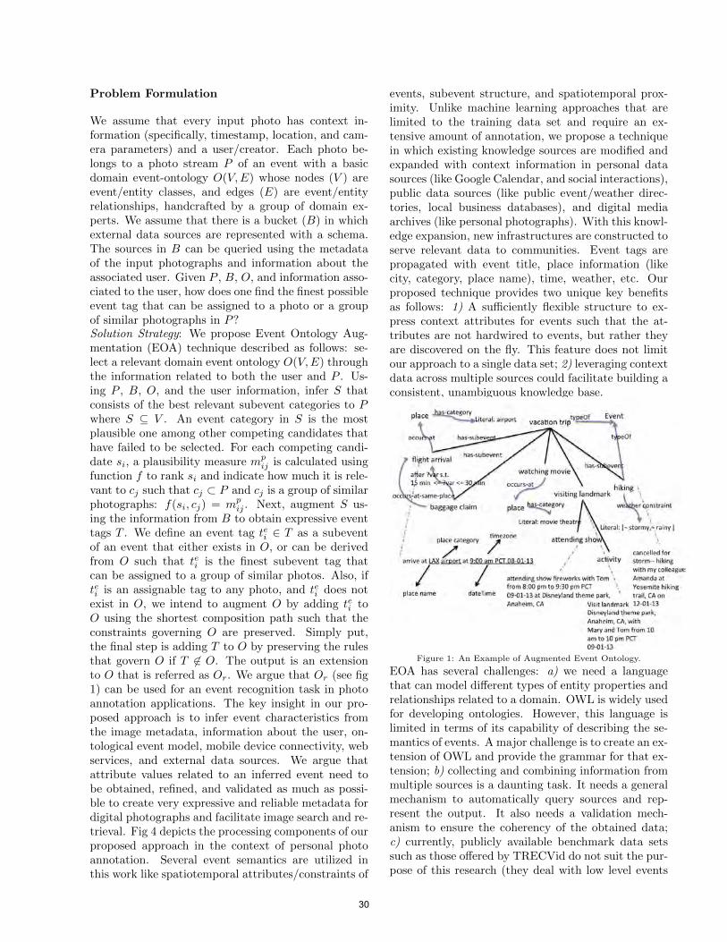
Problem Formulation

We assume that every input photo has context in-formation (specifically, timestamp, location, and cam-era parameters) and a user/creator. Each photo be-longs to a photo stream P of an event with a basicdomain event-ontology O(V,E) whose nodes (V ) areevent/entity classes, and edges (E) are event/entityrelationships, handcrafted by a group of domain ex-perts. We assume that there is a bucket (B) in whichexternal data sources are represented with a schema.The sources in B can be queried using the metadataof the input photographs and information about theassociated user. Given P , B, O, and information asso-ciated to the user, how does one find the finest possibleevent tag that can be assigned to a photo or a groupof similar photographs in P?Solution Strategy: We propose Event Ontology Aug-mentation (EOA) technique described as follows: se-lect a relevant domain event ontology O(V,E) throughthe information related to both the user and P . Us-ing P , B, O, and the user information, infer S thatconsists of the best relevant subevent categories to Pwhere S ⊆ V . An event category in S is the mostplausible one among other competing candidates thathave failed to be selected. For each competing candi-date si, a plausibility measure mp

ij is calculated usingfunction f to rank si and indicate how much it is rele-vant to cj such that cj ⊂ P and cj is a group of similarphotographs: f(si, cj) = mp

ij . Next, augment S us-ing the information from B to obtain expressive eventtags T . We define an event tag tei ∈ T as a subeventof an event that either exists in O, or can be derivedfrom O such that tei is the finest subevent tag thatcan be assigned to a group of similar photos. Also, iftei is an assignable tag to any photo, and tei does notexist in O, we intend to augment O by adding tei toO using the shortest composition path such that theconstraints governing O are preserved. Simply put,the final step is adding T to O by preserving the rulesthat govern O if T 6∈ O. The output is an extensionto O that is referred as Or. We argue that Or (see fig1) can be used for an event recognition task in photoannotation applications. The key insight in our pro-posed approach is to infer event characteristics fromthe image metadata, information about the user, on-tological event model, mobile device connectivity, webservices, and external data sources. We argue thatattribute values related to an inferred event need tobe obtained, refined, and validated as much as possi-ble to create very expressive and reliable metadata fordigital photographs and facilitate image search and re-trieval. Fig 4 depicts the processing components of ourproposed approach in the context of personal photoannotation. Several event semantics are utilized inthis work like spatiotemporal attributes/constraints of

events, subevent structure, and spatiotemporal prox-imity. Unlike machine learning approaches that arelimited to the training data set and require an ex-tensive amount of annotation, we propose a techniquein which existing knowledge sources are modified andexpanded with context information in personal datasources (like Google Calendar, and social interactions),public data sources (like public event/weather direc-tories, local business databases), and digital mediaarchives (like personal photographs). With this knowl-edge expansion, new infrastructures are constructed toserve relevant data to communities. Event tags arepropagated with event title, place information (likecity, category, place name), time, weather, etc. Ourproposed technique provides two unique key benefitsas follows: 1) A sufficiently flexible structure to ex-press context attributes for events such that the at-tributes are not hardwired to events, but rather theyare discovered on the fly. This feature does not limitour approach to a single data set; 2) leveraging contextdata across multiple sources could facilitate building aconsistent, unambiguous knowledge base.

Figure 1: An Example of Augmented Event Ontology.

EOA has several challenges: a) we need a languagethat can model different types of entity properties andrelationships related to a domain. OWL is widely usedfor developing ontologies. However, this language islimited in terms of its capability of describing the se-mantics of events. A major challenge is to create an ex-tension of OWL and provide the grammar for that ex-tension; b) collecting and combining information frommultiple sources is a daunting task. It needs a generalmechanism to automatically query sources and rep-resent the output. It also needs a validation mech-anism to ensure the coherency of the obtained data;c) currently, publicly available benchmark data setssuch as those offered by TRECVid do not suit the pur-pose of this research (they deal with low level events

30

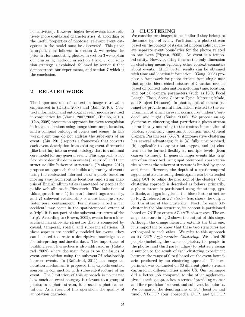
i.e.,activities). However, higher-level events have rela-tively more contextual characteristics; d) according tothe useful properties of photoset, relevant event cat-egories in the model must be discovered. This paperis organized as follows: in section 2, we review theprior art for annotating photos; in section 3 we explainour clustering method; in section 4 and 5, our solu-tion strategy is explained; followed by section 6 thatdemonstrates our experiments, and section 7 which isthe conclusion.

2 RELATED WORK

The important role of context in image retrieval isemphasized in (Datta, 2008) and (Jain, 2010). Con-text information and ontological event models are usedin conjunction by (Viana, 2007,2008), (Fialho, 2010).(Cao, 2008) presents an approach for event recognitionin image collections using image timestamp, location,and a compact ontology of events and scenes. In thiswork, event tags do not address the subevents of anevent. (Liu, 2011) reports a framework that convertseach event description from existing event directories(like Last.fm) into an event ontology that is a minimalcore model for any general event. This approach is notflexible to describe domain events (like ’trip’) and theirstructure (like ’subevent’ structure). (Paniagua, 2012)propose an approach that builds a hierarchy of eventsusing the contextual information of a photo based onmoving away from routine locations, and string anal-ysis of English album titles (annotated by people) forpublic web albums in Picasaweb. The limitations ofthis approach are: 1) human-induced tags are noisy,and 2) subevent relationship is more than just spa-tiotemporal containment. For instance, albeit a ’caraccident’ may occur in the spatiotemporal extent ofa ’trip’, it is not part of the subevent-structure of the’trip’. According to (Brown, 2005), events form a hier-archical narrative-like structure that is connected bycausal, temporal, spatial and subevent relations. Ifthese aspects are carefully modeled for events, theycan be used to create a descriptive knowledge basefor interpreting multimedia data. The importance ofbuilding event hierarchies is also addressed in (Rafati-rad, 2009) where the main focus is on the issues ofevent composition using the subeventOf relationshipbetween events. In (Rafatirad, 2011), an image an-notation mechanism is proposed that exploits contextsources in conjunction with subevent-structure of anevent. The limitation of this approach is no matterhow much an event category is relevant to a group ofphotos in a photo stream, it is used in photo anno-tation. As a result of this operation, the quality ofannotation degrades.

3 CLUSTERINGWe consider two images to be similar if they belong tothe same type of event. Partitioning a photo streambased on the context of its digital photographs can cre-ate separate event boundaries for the photos relatedto one event (Pigeau, 2005). An event is a tempo-ral entity. However, using time as the only dimensionin clustering means ignoring other context semanticsabout events. Much better results can be obtainedwith time and location information. (Gong, 2008) pro-pose a framework for photo stream from single userthat applies hierarchical mixture of Gaussian modelsbased on context information including time, location,and optical camera parameters (such as ISO, FocalLength, Flash, Scene Capture Type, Metering Mode,and Subject Distance). In photos, optical camera pa-rameters provide useful information related to the en-vironment at which an event occurs, like ’indoor’, ’out-door’, and ’night’ (Sinha, 2008). We propose an ag-glomerative clustering that partitions a photo streamhierarchically according to the context information ofphotos, specifically timestamp, location, and OpticalCamera Parameters (OCP). Agglomerative clusteringhas several advantages; it is (a) fully unsupervised,(b) applicable to any attribute types, and (c) clus-ters can be formed flexibly at multiple levels (fromcoarser to finer). In general, larger events like ’trip’are often described using spatiotemporal characteris-tics whereas the subevent structure is limited by spaceand time. However, the depth of a spatiotemporalagglomerative clustering dendrogram can be extendedusing OCP to refine the precision of the clusters. Ourclustering approach is described as follows: primarily,a photo stream is partitioned using timestamp, gps-latitude, and gps-longitude; the blue cluster structurein Fig 2, referred as ST-cluster tree, shows the outputfor this stage of the clustering. Next, for each ST-cluster in the blue structure, its content is partitionedbased on OCP to create ST-OCP cluster tree. The or-ange structure in fig 2 shows the output of this stage.Although the orange hierarchy extends the blue one,it is important to know that these two structures areorthogonal to each other. We refer to this approachas ST-OCP Agglomerative Clustering. We asked 20people (including the owner of photos, the people inthe photos, and third party judges) to relatively assigna number to the result of each clustering experimentbetween the range of 0 to 6 based on the event bound-aries produced by our clustering approach. This ex-periment was conducted on 30 different photo streamscaptured in different cities inside US. Our techniquedid a better job compared to the other agglomera-tive clustering approaches in terms of providing coarserand finer precision for event and subevent boundaries.We compared the dendrograms of ST (location andtime), ST-OCP (our approach), OCP, and STOCP

31

clustering (in which location and time and OCP at-tributes are used together in the distance function).The arrangement of clusters depends on the image at-tributes used in the clustering. The photos are sortedin chronological order. Image content features arenot used in these cluster arrangements. The equation’OCP ≺ S ≺ T ≺ STOCP ≺ ST ≺ ST − OCP ’ showsthat the arrangement of clusters improved from left toright — S and T, respectively, mean that agglomera-tive clustering is conducted using the location, and thetimestamp attributes of photos. We used single link-age clustering and Euclidean distance in our clusteringtechnique. However, one can use other approaches andrefine the results.

Figure 2: ST-OCP Agglomerative Clustering.

4 EOAWe present the observations with a set of descriptors.Each descriptor is a formula for a photo or a cluster —a cluster is a group of contextually similar photos. Inthis section, we show that it is feasible to go from a setof descriptors D to the best subevent category, whenthe following conditions are satisfied: (a) the descrip-tors in D are consistent among themselves, (b) the de-scriptors in D satisfy subevent categories, (c) axiomsof a subevent category are consistently formulated inan event ontology, and (d) the inferred subevent cate-gories are sound and complete.

4.1 EVENT MODELWe use a basic derivation of E* model (Gupta, 2011)as our core event model, to specify the general relation-ships between events and entities. Specifically, we uti-lized the relationships subeventOf, which specifies theevent structure and event containment. The expres-sion e1 subeventOf e2 indicates that e1 occurs withinthe spatiotemporal bounds of e2, and e1 is part ofthe regular structure of e2. Additionally, we used thespatiotemporal relationships like occurs-during andoccurs-at to specify the space and time properties ofan event. The time and space model in this workis mostly derived from E*. We use the relationshipsco-occurring-with, and co-located-with, spatially-near,temporal-overlap , before, and after to describe thespatiotemporal neighborhood of an event. We usedseveral other relationships to describe additional con-straints about events (e.g., e1 has-ambient-constraint

A, and A has-value indoor). To express a certaingroup of temporal constraints, we utilized some ofLinear Temporal Logic, Metric Temporal Logic, andReal-Time Temporal Logic formulas (Koymans, 1990),(Alur, 1991). We developed a language L with a syn-tax and grammar as an extension to OWL to embracecomplex temporal formulas. Further, we extended thelanguage to support a combination of classical propo-sitional operators, linear spatial constraints, and spa-tial distance functions which can not be expressed inOWL; equation feucDist(e1, e2,@ ≤ 100) shows a rel-ative spatial constraint in L, which states the evente1 occurs at most 100 meters away from the place atwhich event e2 occurs.

Domain Event OntologyA domain event ontology provides specialized taxon-omy for a certain domain like trip, see fig 3. The Mis-cellaneous subevent category in this model is used toannotate the photos that are not matched with anyother category. The general vocabulary in a core eventmodel is reused in a domain event ontology. For in-stance, Parking in fig 3, is a subClassOf of Occurrent(or event) concept in the core event ontology. Also,relationships like subeventOf are reused from the coreevent ontology. We assume that domain event ontolo-gies are handcrafted by a group of domain experts.

4.2 DESCRIPTOR REPRESENTATIONMODEL

We represent a descriptor using the schema in scripttyped : valued, confidenced : val, in which typed,valued, and val indicate the type, value,and certainty(between 0 and 1) of the descriptor, respectively. Forinstance, the descriptor Flash : ‘off ‘, confidence :1.0 for a photo, states that the flash was off whenthe photo was captured with 100% certainty. Photoand cluster descriptors follow the same representationmodel, however the rules for computing the value ofconfidenced are different. We will describe these rulesin the following paragraphs. The descriptor model ofa cluster includes two fields in addition to that of aphoto: plausibility-weight ≥ 0 , and implausibility-weight < 0. Later, we will explain the usage of thesefields. All descriptors are either direct or derived. Forphoto descriptors, by convention, we assume that a di-rect descriptor is straightly extracted from the EXIFmetadata of a photo, and its confidence is 1, as in theabove example. The direct descriptors that we usedin this paper are related to time, location, and opti-cal parameters of photos like GPSLatitude ,GPSLon-gitude , Orientation, Timestamp, and ExposureTime.For a derived descriptor like sceneType : ‘indoor‘,confidence : 0.6, the descriptor value ‘indoor‘ is com-puted using direct descriptors like Flash, through a se-quence of computations that extract information froma bucket of data sources. Some of these descriptors arePlaceCategory1, and HoursOfOperation2. The confi-dence score is obtained from the processing unit used

1The nearest local business category to a photo’s location.

2The hours during which a local business is open.

32

to compute the descriptor value — we developed sev-eral information retrieval algorithms for this purposeincluding the tools in our lab (Sinha, 2008). If a de-scriptor value is directly extracted from an externaldata source, confidenced is equal to 1. Direct descrip-tors of a cluster must represent all photos containedin it; some of these descriptors represent boundingbox,time-interval, and size of the cluster. The confidencevalue for direct descriptors is equal to 1, for instance,the descriptor size : 5, confidenced : 1.0 indicatesthe number of photos in a cluster. Given a photo piin a photo stream P , and the cluster c that groups piwith the most similar photos in P , a processing unitproduces the descriptors of c using the descriptors ofthe photos in c, and more importantly, this process isguided by the descriptors of pi. Every photo in c mustsupport every derived descriptor of pi; such cluster isreferred as a sound cluster for pi, and the derived de-scriptors for c are represented by the distinct union ofthe derived descriptors of the photos in c. For a de-rived cluster descriptor d, the value of confidenced iscalculated using the formula in equation 1, in which|c| is the size of the cluster, pj is every photo in c thatis represented by d, and g(pj , d) gives the confidencevalue of d in pj . To find a sound cluster for a photo,the hierarchical structure that is produced by the clus-tering unit, is traversed using depth-first search — thehalting condition for this navigation, if no sound clus-ter was found, is when current cluster is a leaf node.

confidenced =1

|c|×

∑g(pj , d) (1)

Descriptor ConsistencyConsistency among a set of descriptors is a manda-tory condition to infer the best possible conclu-sion from it. We make sure that consistency ex-ists among the descriptors of a photo as well asthe descriptors of a cluster, using entailment rulesdescribed below. (a) vi → vk: if vi implies vk,then the rules for vk must also be applied to vi.This is referred as transitive entailment rule. Forinstance, suppose a photo/cluster has the followingdescription, ′outdoorSeating : true′ ; ′sceneType :outdoor′; ′weatherCondition : storm′, which impliesthat the nearest local business (e.g. restaurant) to thephoto/cluster, offers outdoorSeating, and the weatherwas stormy when the photo(s) were captured. Giventhe sequence of rules below,outdoorSeating ∧ outdoor → fineWeather; fineWeather → ¬storm

rule outdoorSeating ∧ outdoor → ¬storm is entailed thatindicates an inconsistency among the descriptors of aphoto/cluster. (b) vi → funcremove(vk): vi impliesremoving the descriptor vk. This is referred as a de-terministic entailment rule. (c) vi∧vk → truth value:rules of this type are referred as non-deterministic en-tailment rules in which the inconsistency is expressedby a false truth value e.g. closeShot ∧ landscape →false. In that case, further decisions on keep-ing,modifying, or discarding either of the descriptorsvi or vk will be based on the confidence value as-signed to each descriptor — this operation is referredas update, which is executed when an inconsistency oc-curs between two candidate descriptors. The followingrules are used by this process: (a) for two descriptors

with the same type, the descriptor with lower confi-dence score is discarded, (b) for two descriptors withdifferent types, the one with lower confidence scoregets modified until the descriptors are consistent. Themodification is defined as either negation or expan-sion within the search space. In case of negation, e.g.¬outdoor → indoor, the confidence value for indoordescriptor is calculated by subtracting the confidencevalue of outdoor descriptor from 1. An example of ex-pansion is increasing a window size to discover morelocal businesses near a location. To avoid falling in-side an infinite loop, we limit the count of negation,and the size of search space during expansion, by athreshold. We assign null to the descriptor that hasalready reached a threshold and is still inconsistent.null is universally consistent with any descriptor. Thevocabulary that is used to model the descriptors fora photo/cluster is taken from the vocabulary that isspecified in the core event model.

4.3 BUCKET OF DATA SOURCESWe represent each data source with a declarativeschema, using the vocabulary of the core event model.This schema indicates the type of source output, aswell as the type of input attributes a source needs todeliver the output. Data sources are queried using theSPARQL language. The following script shows an ex-ample used to query a source; var1 is a query variable(output that must be delivered by the source); attr1

is the input attribute of the source; classw indicates aclass type, and rela indicates a relationship. The classtypes and relationships used in such queries are con-structed using the vocabulary of the core event model.SELECT ?var1 FROM < SourceURI > WHEREattr1 core : typeOf classw; var1 core : typeOf classu;

?var1 core : rela ?x; ?x core : relb ?y; ?y core : reld attr1.

The above query is constructed automatically usingthe schema of data sources, and the available infor-mation. Simply put, a source is selected if its inputattributes match the available information I. At ev-ery iteration, I is incrementally updated with new datathat is delivered by a source. The next source is se-lected if its input attributes are included in I. Thisprocess continues until no more source with matchingattributes is left in the bucket B.

4.4 EVENT INFERENCEFrom a set of consistent cluster descriptors (observa-tions), we developed an algorithm to infer the mostplausible subevent category described in a domainevent ontology. This algorithm, uses the domain eventmodel, which is a graph; we represent this graphwith the notation O(V,E) in which V includes eventclasses, and E includes event relationships. Travers-ing the event graph O starts with the root of hierar-chical subevent structure. The algorithm visits eventcandidates in E through some of the relationshipsin E like subeventOf, co-occurring-with, co-located-with, spatially-near, temporal-overlap, before, and af-ter — these relationships help to reach other event

33

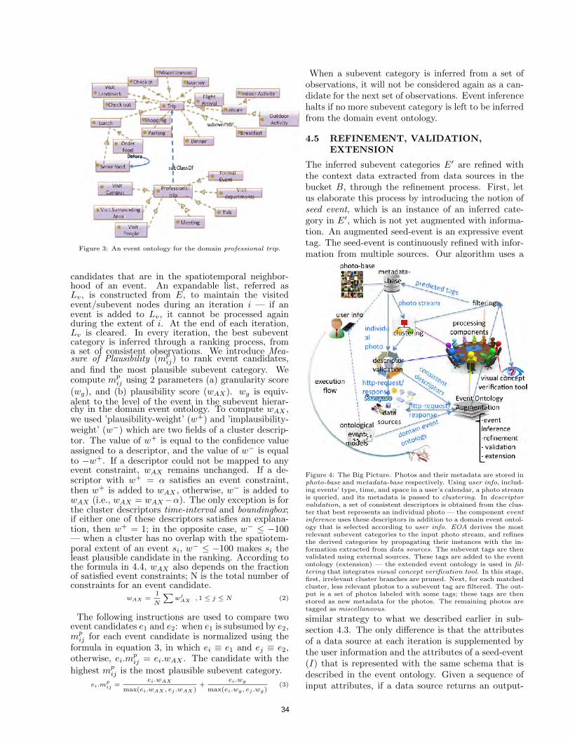
Figure 3: An event ontology for the domain professional trip.

candidates that are in the spatiotemporal neighbor-hood of an event. An expandable list, referred asLv, is constructed from E, to maintain the visitedevent/subevent nodes during an iteration i — if anevent is added to Lv, it cannot be processed againduring the extent of i. At the end of each iteration,Lv is cleared. In every iteration, the best subeventcategory is inferred through a ranking process, froma set of consistent observations. We introduce Mea-sure of Plausibility (mp

ij) to rank event candidates,and find the most plausible subevent category. Wecompute mp

ij using 2 parameters (a) granularity score

(wg), and (b) plausibility score (wAX). wg is equiv-alent to the level of the event in the subevent hierar-chy in the domain event ontology. To compute wAX ,we used ’plausibility-weight’ (w+) and ’implausibility-weight’ (w−) which are two fields of a cluster descrip-tor. The value of w+ is equal to the confidence valueassigned to a descriptor, and the value of w− is equalto −w+. If a descriptor could not be mapped to anyevent constraint, wAX remains unchanged. If a de-scriptor with w+ = α satisfies an event constraint,then w+ is added to wAX , otherwise, w− is added towAX (i.e., wAX = wAX−α). The only exception is forthe cluster descriptors time-interval and boundingbox;if either one of these descriptors satisfies an explana-tion, then w+ = 1; in the opposite case, w− ≤ −100— when a cluster has no overlap with the spatiotem-poral extent of an event si, w

− ≤ −100 makes si theleast plausible candidate in the ranking. According tothe formula in 4.4, wAX also depends on the fractionof satisfied event constraints; N is the total number ofconstraints for an event candidate.

wAX =1

N

∑w

jAX , 1 ≤ j ≤ N (2)

The following instructions are used to compare twoevent candidates e1 and e2: when e1 is subsumed by e2,mp

ij for each event candidate is normalized using theformula in equation 3, in which ei ≡ e1 and ej ≡ e2,otherwise, ei.m

pij = ei.wAX . The candidate with the

highest mpij is the most plausible subevent category.

ei.mpij =

ei.wAX

max(ei.wAX , ej .wAX)+

ei.wg

max(ei.wg, ej .wg)(3)

When a subevent category is inferred from a set ofobservations, it will not be considered again as a can-didate for the next set of observations. Event inferencehalts if no more subevent category is left to be inferredfrom the domain event ontology.

4.5 REFINEMENT, VALIDATION,EXTENSION

The inferred subevent categories E′ are refined withthe context data extracted from data sources in thebucket B, through the refinement process. First, letus elaborate this process by introducing the notion ofseed event, which is an instance of an inferred cate-gory in E′, which is not yet augmented with informa-tion. An augmented seed-event is an expressive eventtag. The seed-event is continuously refined with infor-mation from multiple sources. Our algorithm uses a

Figure 4: The Big Picture. Photos and their metadata are stored inphoto-base and metadata-base respectively. Using user info, includ-ing events’ type, time, and space in a user’s calendar, a photo streamis queried, and its metadata is passed to clustering. In descriptorvalidation, a set of consistent descriptors is obtained from the clus-ter that best represents an individual photo — the component eventinference uses these descriptors in addition to a domain event ontol-ogy that is selected according to user info. EOA derives the mostrelevant subevent categories to the input photo stream, and refinesthe derived categories by propagating their instances with the in-formation extracted from data sources. The subevent tags are thenvalidated using external sources. These tags are added to the eventontology (extension) — the extended event ontology is used in fil-tering that integrates visual concept verification tool. In this stage,first, irrelevant cluster branches are pruned. Next, for each matchedcluster, less relevant photos to a subevent tag are filtered. The out-put is a set of photos labeled with some tags; these tags are thenstored as new metadata for the photos. The remaining photos aretagged as miscellaneous.

similar strategy to what we described earlier in sub-section 4.3. The only difference is that the attributesof a data source at each iteration is supplemented bythe user information and the attributes of a seed-event(I) that is represented with the same schema that isdescribed in the event ontology. Given a sequence ofinput attributes, if a data source returns an output-

34

array of size K, then our algorithm creates K newinstances of events with the same type as in the seed-event, and augments them with the information in theoutput-array. The augmented seed-events are addedto I for the next iteration; I is constantly updated un-til all the event categories in E′ are augmented, and/orthere is no more data source (in the bucketB) to query.To avoid falling into an infinite loop of querying datasources, we set the following condition: a data sourcecannot be queried more than once for each seed-event.We defined some queries manually that are expressedthrough the relative spatiotemporal relationships inthe event ontology, and the augmented seed-events;these queries are used to augment the seed-events withrelative spatiotemporal properties. When a seed-eventgets augmented with information, our technique val-idates the event tag by using the event constraints,augmented event attributes, and a sequence of entail-ment rules that specify the cancel status for an event.For instance, if the weather attribute for an event isheavy rain, and the weather constraint fine weatheris defined for an event, then the status of the eventtag becomes canceled. After the validation, event tagsare added to the domain event ontology by extendingevent classes through typeOf relationship. This stepproduces an augmented event ontology that is the ex-tended version of the prior model (see fig 1).

5 FILTERINGFiltering is a two-step process; (1) redundant and irrel-evant clusters are pruned from the hierarchical clusterstructure produced by the clustering component, seefig 5-step-1. Equation 4 describes the prune-rule, andmatch-rule in this step. traverse-rule in equation 4 isused to visit cluster nodes— c implies cluster.

¬InsideST (tage , c)→ Prune(c). (4)

InsideST (c , tage)→Match(c, tage). (5)

InsideST (tage, c) ∧ hasChild(c)→ Trvs(c.child). (6)

(2) filter redundant photos from the matched cluster,see fig 5-step-2. This is accomplished by applying thecontext and visual constraints of the expressive tagthat is matched to the cluster. We used a concept ver-ification tool3 to verify the visual constraints of eventsusing image features. This tool uses pyramids of colorhistogram and GIST features. Filtering operation isdeeply guided by the expressive tags. During this op-eration, subevent relations are used for navigating theaugmented event model.

6 EXPERIMENTAL EVALUATIONSWe focused on 3 domain scenarios vacation, profes-sional trip, and wedding.

6.0.1 Experimental Data Set

We crawled Flickr, Picasaweb, and our lab data sets.Based on the assumption that people store their per-

3http://socrates.ics.uci.edu/Pictorria/public/demo

Figure 5: Filtering Operation.

sonal photos according to events,we collected the datasets based on time, space, and event types (like travel,conference, meeting, workshop, vacation, and wed-ding). We developed some crawlers to download about700 albums of the day’s featured photos. In addition,we crawled photo albums uploaded since the year 2010;the reason was that most of the older collections didnot contain geo-tagged photos. After 4 months, we col-lected 84,021 albums (about 6M photos) from whichonly 570 albums (about 60K photos) had the requiredEXIF information containing location, timestamp, andoptical camera parameters. We ignored the albums a)smaller than 30 photos, b) with non-English annota-tions. The average number of photos per album was105. We used the albums from the most active usersbased on the amount of user annotation; we endedup with a diverse collection of 20 users with heteroge-neous photo albums in terms of time period and ge-ographical sparseness. The geographic sparseness ofalbums ranged from being across continents, to citiesof the same country/state. Some of the users return toprior locations, and some do not. Fig 6 sketches thegeographic distribution of our data set. We noticedthat data sources do not equally support all the ge-ographic regions; for instance,only a small number ofdata sources supported the data sets captured insideIndia. The photos for vacation/professional-trip do-mains have higher temporal and geographical sparse-ness compared to photos related to wedding domain.The number of albums for vacation domain exceedsthe other two.

6.0.2 Experimental Set-Up

We picked the 4 most active users (based on theamount of user annotation) from our non-lab, down-loaded data set, and 2 most active users from our labdata set (based on the number of collections they own).As ground-truth for the lab data set, we asked the

35

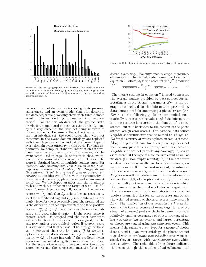
Figure 6: Data set geographical distribution. The black bars showthe number of albums in each geographic region, and the gray barsshow the number of data sources that supported the correspondinggeographic region.

owners to annotate the photos using their personalexperiences, and an event model that best describesthe data set, while providing them with three domainevent ontologies (wedding, professional trip, and va-cation). For the non-lab data set, the ground truthprovides a manual and subjective event labeling doneby the very owner of the data set being unaware ofthe experiments. Because of the subjective nature ofthe non-lab data set, the event types that were notcontained in the event domain ontology are replacedwith event type miscellaneous that is an event type inevery domain event ontology in this work. For each ex-periment, we compute standard information retrievalmeasures (precision, recall, and F1-measure), for theevent types used in tags. In addition to that, we in-troduce a measure of correctness for event tags. Thescore is obtained based on multiple context cues. Forinstance, label meeting with Tom Johnson at RA SushiJapanese Restaurant in Broadway, San Diego, duringtime interval ”blah” in a sunny day, in an outdoor en-vironment, specifies type of the event, its granularity inthe subevent hierarchy, place, time, and environmentcondition. We developed an algorithm that evaluateseach cue with a number in the range of 0 to 1 as fol-lows: 1) event type: wrong = 0, correct = 1, somehow

correct =Lp

LTPsuch that Lp is the subevent-granularity

level for a predicted tag and LTP is the subevent gran-ularity level for the true-positive tag (the predicted tagis the direct or indirect superevent of the true-positive

tag i.e.,Lp

LTP≤ 1); 2) place: includes place name, cat-

egory and geographical region. If the place name iscorrect, score 1 is assigned and the other attributeswill not be checked. Otherwise, 0 is assigned; for thecategory and/or geographical region if correct, score1 is assigned, and 0 otherwise. The average of thesevalues represent the score for place; 3) for weather,optical, and visual constraint: wrong=0, correct =1,unsure = 0.5; 4) time interval: if the predicted eventtag occurs anytime during the true-positive event tag,1 is the score, otherwise 0. The average of the abovescores represents the correctness measure for a pre-

Figure 7: Role of context in improving the correctness of event tags.

dicted event tag. We introduce average correctnessof annotation that is calculated using the formula inequation 7, where wj is the score for the jth predictedtag.

correctness =

∑Lj=1 wj

L; context = 1− Err (7)

The metric context in equation 7 is used to measurethe average context provided by data sources for an-notating a photo stream; parameter Err is the av-erage error related to the information provided bydata sources used for annotating a photo stream (0 ≤Err ≤ 1); the following guidelines are applied auto-matically, to measure this value: (a) if the informationin a data source is related to the domain of a photostream, but it is irrelevant to the context of the photostream, assign error-score 1. For instance, data sourceTripAdvisor returns zero results related to Things-To-Do for the country at which a photo stream is created.Also, if a photo stream for a vacation trip does notinclude any picture taken in any landmark location,TripAdvisor does not provide any coverage; (b) assignerror-score 0 if the type of a source is relevant as well asits data (i.e. non-empty results); (c) if the data froma relevant source is insufficient for a photo stream, as-sign error-score 0.5. For instance, only a subset ofbusiness venues in a region are listed in data sourceYelp; as a result, the data source returns informationfor less than 30% of the photo stream; (d) for a datasource, multiply the error-score by a fraction in whichthe numerator is the number of photos tagged usingthis data source, and the denominator is the size of thephoto stream. Do this for all the sources and obtainthe weighted average of the error-scores. The result isErr. The implication of our result in fig 7 is as fol-lows: while the correctness of event tags (for a photostream of an event) peaks with the increase in context,relatively, smaller percentage of photos are tagged us-ing non-miscellaneous events, and larger percentageof photos are tagged using miscellaneous event. Thismeans if the suitable event type for a group of photosdoes not exist in an event ontology, the photos are nottagged with an irrelevant non-miscellaneous event; in-stead, they are tagged with miscellaneous event whichmeans other. The right side of the figure indicatesthat even though the number of miscellaneous and

36

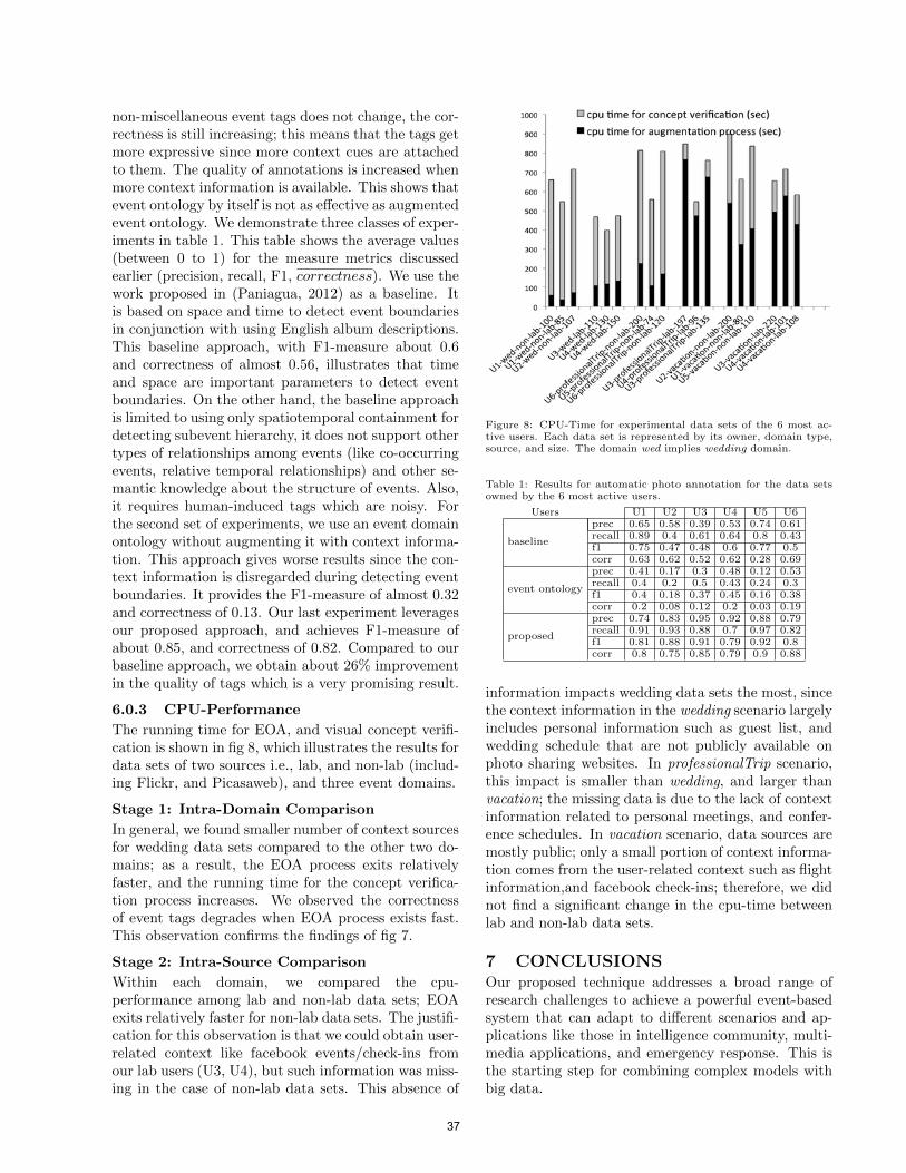
non-miscellaneous event tags does not change, the cor-rectness is still increasing; this means that the tags getmore expressive since more context cues are attachedto them. The quality of annotations is increased whenmore context information is available. This shows thatevent ontology by itself is not as effective as augmentedevent ontology. We demonstrate three classes of exper-iments in table 1. This table shows the average values(between 0 to 1) for the measure metrics discussedearlier (precision, recall, F1, correctness). We use thework proposed in (Paniagua, 2012) as a baseline. Itis based on space and time to detect event boundariesin conjunction with using English album descriptions.This baseline approach, with F1-measure about 0.6and correctness of almost 0.56, illustrates that timeand space are important parameters to detect eventboundaries. On the other hand, the baseline approachis limited to using only spatiotemporal containment fordetecting subevent hierarchy, it does not support othertypes of relationships among events (like co-occurringevents, relative temporal relationships) and other se-mantic knowledge about the structure of events. Also,it requires human-induced tags which are noisy. Forthe second set of experiments, we use an event domainontology without augmenting it with context informa-tion. This approach gives worse results since the con-text information is disregarded during detecting eventboundaries. It provides the F1-measure of almost 0.32and correctness of 0.13. Our last experiment leveragesour proposed approach, and achieves F1-measure ofabout 0.85, and correctness of 0.82. Compared to ourbaseline approach, we obtain about 26% improvementin the quality of tags which is a very promising result.

6.0.3 CPU-Performance

The running time for EOA, and visual concept verifi-cation is shown in fig 8, which illustrates the results fordata sets of two sources i.e., lab, and non-lab (includ-ing Flickr, and Picasaweb), and three event domains.

Stage 1: Intra-Domain Comparison

In general, we found smaller number of context sourcesfor wedding data sets compared to the other two do-mains; as a result, the EOA process exits relativelyfaster, and the running time for the concept verifica-tion process increases. We observed the correctnessof event tags degrades when EOA process exists fast.This observation confirms the findings of fig 7.

Stage 2: Intra-Source Comparison

Within each domain, we compared the cpu-performance among lab and non-lab data sets; EOAexits relatively faster for non-lab data sets. The justifi-cation for this observation is that we could obtain user-related context like facebook events/check-ins fromour lab users (U3, U4), but such information was miss-ing in the case of non-lab data sets. This absence of

Figure 8: CPU-Time for experimental data sets of the 6 most ac-tive users. Each data set is represented by its owner, domain type,source, and size. The domain wed implies wedding domain.

Table 1: Results for automatic photo annotation for the data setsowned by the 6 most active users.

Users U1 U2 U3 U4 U5 U6

baseline

prec 0.65 0.58 0.39 0.53 0.74 0.61recall 0.89 0.4 0.61 0.64 0.8 0.43f1 0.75 0.47 0.48 0.6 0.77 0.5corr 0.63 0.62 0.52 0.62 0.28 0.69

event ontology


proposed


information impacts wedding data sets the most, sincethe context information in the wedding scenario largelyincludes personal information such as guest list, andwedding schedule that are not publicly available onphoto sharing websites. In professionalTrip scenario,this impact is smaller than wedding, and larger thanvacation; the missing data is due to the lack of contextinformation related to personal meetings, and confer-ence schedules. In vacation scenario, data sources aremostly public; only a small portion of context informa-tion comes from the user-related context such as flightinformation,and facebook check-ins; therefore, we didnot find a significant change in the cpu-time betweenlab and non-lab data sets.

7 CONCLUSIONSOur proposed technique addresses a broad range ofresearch challenges to achieve a powerful event-basedsystem that can adapt to different scenarios and ap-plications like those in intelligence community, multi-media applications, and emergency response. This isthe starting step for combining complex models withbig data.

37

References

M. Naaman, S. Harada, Q.Y. Wang, H. Garcia-Molina,and A. Paepcke (2004). Context data in geo-referenceddigital photo collections. In Proceedings of the 12thannual ACM international conference on Multimedia.

M. Naaman, Y.J. Song, A. Paepcke, and H. Garcia-Molina (2004). Automatic organization for digitalphotographs with geographic coordinates. Digital Li-braries. In Proceedings of the 2004 Joint ACM/IEEEConference.

R. Datta, D. Joshi,J. Li, and J.Z. Wang (2008). Im-age retrieval: Ideas, influences, and trends of the newage, ACM Computing Surveys (CSUR).

R. Jain, and P. Sinha (2010). Content without con-text is meaningless, Proceedings of the internationalconference on Multimedia, ACM.

W. Viana, J.Filho, J.Gensel, M. Villanova Oliver, andH.Martin (2007). PhotoMap–Automatic Spatiotempo-ral Annotation for Mobile Photos, Web and WirelessGeographical Information Systems, Springer.

W. Viana, J. Bringel Filho,J. Gensel,M. Villanova-Oliver,and H. Martin (2008). PhotoMap: from lo-cation and time to context-aware photo annotations,Journal of Location Based Services, Taylor & Francis.

X. Liu, R. Troncy, and B. Huet (2011). Finding mediaillustrating events, Proceedings of the 1st ACM Inter-national Conference on Multimedia Retrieval.

A. Fialho, R. Troncy, L. Hardman, C. Saathoff, andA. Scherp (2010). What’s on this evening? Design-ing User Support for Event-based Annotation and Ex-ploration of Media, 1st International Workshop onEVENTS-Recognising and tracking events on the Weband in real life.

L. Cao, J. Luo, H. Kautz, and T.S. Huang (2008).Annotating collections of photos using hierarchicalevent and scene models, Computer Vision and PatternRecognition, 2008. CVPR 2008. IEEE Conference.

J. Paniagua, I. Tankoyeu, J. Stottinger, andF. Giunchiglia (2012). Indexing media by personalevents, Proceedings of the 2nd ACM InternationalConference on Multimedia Retrieval.

N.R. Brown (2005). On the prevalence of event clus-ters in autobiographical memory, Social Cognition,Guilford Press.

A. Pigeau, and M. Gelgon (2005). Building and track-ing hierarchical geographical & temporal partitions forimage collection management on mobile devices, Pro-ceedings of the 13th annual ACM international confer-ence on Multimedia.

B. Gong, U. Westermann, S. Agaram, and R. Jain(2006). Event Discovery in Multimedia Reconnais-

sance Data Using Spatio-Temporal Clustering, Pro-ceeding of the AAAI Workshop on Event Extractionand Synthesis.

B. Gong, and R. Jain (2008). Hierarchical photostream segmentation using context, Proceedings ofSPIE, Multimedia content Access: Algorithms andSystem.

P. Sinha, and R. Jain (2008). Classification and an-notation of digital photos using optical context data,CIVR.

A. Gupta, and R. Jain (2011). Managing Event Infor-mation: Modeling, Retrieval, and Applications, Syn-thesis Lectures on Data Management, Morgan & Clay-pool Publishers.

R. Koymans (1990). Specifying real-time propertieswith metric temporal logic, Real-Time Syst.,2(4).

R. Alur and T.A. Henzinger (1991). Logics and mod-els of real time: A survey, J. W de Bakker, C. Huiz-ing, W.P. de Roever, and G. Rozenberg, editors, REXWorkshop, Springer.

S. Rafatirad, A. Gupta, and R. Jain (2009). Eventcomposition operators: ECO, Proceedings of the 1stACM international workshop on Events in multimedia.

S. Rafatirad, and R. Jain (2011). Contextual Augmen-tation of Ontology for Recognizing Sub-events, Seman-tic Computing (ICSC), 2011 Fifth IEEE InternationalConference.

38

Learning Parameters by Prediction Markets and Kelly Rulefor Graphical Models

Wei SunCenter of Excellence

in C4IGeorge Mason University

Fairfax, VA 22030

Robin HansonDepartment of EconomicsGeorge Mason University

Fairfax, VA 22030

Kathryn B. LaskeyDepartment of Systems

Engineering andOperations Research

George Mason UniversityFairfax, VA 22030

Charles TwardyCenter of Excellence

in C4IGeorge Mason University

Fairfax, VA 22030

Abstract

We consider the case where a large numberof human and machine agents collaborate toestimate a joint distribution on events. Someof these agents may be statistical learnersprocessing large volumes of data, but typi-cally any one agent will have access to onlysome of the data sources. Prediction mar-kets have proven to be an accurate and ro-bust mechanism for aggregating such esti-mates (Chen and Pennock, 2010), (Barbuand Lay, 2011). Agents in a prediction mar-ket trade on futures in events of interest.Their trades collectively determine a prob-ability distribution. Crucially, limited trad-ing resources force agents to prioritize ad-justments to the market distribution. Op-timally allocating these resources is a chal-lenging problem. In the economic spirit ofspecialization, we expect prediction marketsto do even better if agents can focus on be-liefs, and hand off those beliefs to an opti-mal trading algorithm. Kelly (1956) solvedthe optimal investment problem for single-asset markets. In previous work, we devel-oped efficient methods to update both thejoint probability distribution and user’s as-sets for the graphical model based predictionmarket (Sun et al., 2012). In this paper wecreate a Kelly rule automated trader for com-binatorial prediction markets and evaluate itsperformance by numerical simulation.

1 INTRODUCTION

There was a time when “big” data meant too big tofit into memory. As memory capacity expanded, whatwas once big became small, and “big” grew ever big-ger. Then came cloud computing and the explosion of

“big” data to a planetary scale. Whatever the scaleof “big,” a learner faced with big data is by defini-tion forced to subsample, use incremental methods, orotherwise specialize. Humans are no strangers to spe-cialization: scientific knowledge alone has exceeded thecapacity of any single head for at least four centuries.In this paper we consider a mechanism for fusing theefforts of many specialized agents attempting to learna joint probability space which is assumed to be largerthan any one of them can encompass. We seek a mech-anism where agents contribute only where they haveexpertise, and where each question gets the input ofmultiple agents. As we discuss below, our mechanismis a kind of prediction market. However, in contrastto (Barbu and Lay, 2011), we wish our human andmachine agents to concentrate on their beliefs, not onplaying the market. Therefore we formulate and de-velop a helper agent which translates partial beliefsinto near-optimal trades in a combinatorial market ofarbitrary size. We do not here actually apply it to abig dataset.

It is well known that prediction accuracy increases asmore human and/or machine forecasters contribute toa forecast (Solomonoff, 1978). While one approach isto ask for and average forecasts from many individu-als, an approach that often works better is to combineforecasts through a prediction market (Chen and Pen-nock, 2010; Barbu and Lay, 2011). In a market-makerbased prediction market, a consensus probability dis-tribution is formed as individuals either edit probabil-ities directly or trade in securities that pay off con-tingent on an event of interest. Combinatorial pre-diction markets allow trading on any event that canbe specified as a combination of a base set of events.However, explicitly representing the full joint distri-bution is infeasible for markets with more than a fewbase events. Tractable computation can be achievedby using a factored representation (Sun et al., 2012).Essentially, the probabilities being edited by users arethe parameters of the underlying graphical model rep-resenting the joint distribution of events of interest. In

39

another words, prediction markets work as a crowd-sourcing tool for learning model parameters from hu-man or automated agents.

Prediction markets appear to achieve improved accu-racy in part because individuals can focus on con-tributing to questions about which they have the mostknowledge, and in part because individuals can learnby watching the trades of others. However, one impor-tant disadvantage of prediction markets is that usersmust figure out how to translate their beliefs intotrades. That is, users must decide when to trade howmuch, and whether to make a new offer or to accept anexisting offer. Prediction markets with market makerscan simplify this task, allowing users to focus on ac-cepting existing offers. Edit-based interfaces can fur-ther simplify the user task, by having users browse forexisting estimates they think are mistaken, and thenspecify new values they think are less mistaken.

However, even with these simplifications, participantsmust think about resources as well as beliefs. For ex-ample, if users just make edits whenever they noticethat market estimates differ from their beliefs, par-ticipants are likely to quickly run out of available re-sources, which will greatly limit their ability to makefurther edits. To avoid this problem, users must tryto keep track of their best opportunities for tradinggains, and avoid or undo trades in other areas in orderto free up resources to support their best trades.

This problem is made worse in combinatorial predic-tion markets. By allowing users to trade on any be-liefs in a large space of combinations of some base setof topics, combinatorial markets allow users to con-tribute much more information, and to better dividetheir labors. But the more possible trades there are,the harder it becomes for users to know which of themany possible trades to actually make.

Ideally, prediction market users could have a tradingtool available to help them manage this process oftranslating beliefs into trades. Users would tell thistool about their beliefs, and the tool would decidewhen to trade how much. But how feasible is sucha tool? One difficulty is that optimal trades dependin principle on expectations about future trading op-portunities. A second difficulty is that users must notonly tell the tool about their current beliefs, they mustalso tell the tool how to change such stated beliefs inresponse to changes in market prices. That is, thetrading tool must learn from prices in some manneranalogous to the way the user would have learned fromsuch prices.

To make this problem manageable, we introduce foursimplifications. First, we set aside the problem of howusers can easily and efficiently specify their current be-

liefs, and assume that a user has somehow specified afull joint probability distribution over some set of vari-ables. Second, we set aside the problem of guessingfuture trading opportunities, by assuming that futureopportunities will be independent of current opportu-nities. Third, we assume that a user can only accepttrade offers made by a continuous market maker, andcannot trade directly with other users. Fourth, we setaside the problem of how a tool can learn from marketprices, by assuming that it would be sufficient for thetool to optimize a simple utility function depending onthe user’s assets and market prices.

Given these assumptions, the prediction market trad-ing tool design problem reduces to deciding what pre-diction market trades to make any given moment,given some user-specified joint probability distributionover a set of variables for which there is a continuouscombinatorial market maker. It turns out that thisproblem has largely been solved in the field of evolu-tionary finance.

That is, if the question is how, given a set of beliefs, toinvest among a set of available assets to minimize one’schances of going broke, and maximize one’s chanceof eventually dominating other investors, the answerhas long been known. The answer is the “Kelly rule”(Kelly, 1956), which invests in each category of as-sets in proportion to its expected distant future frac-tion of wealth, independent of the current price ofthat category. When they compete with other trad-ing rules, it has been shown that Kelly rule traderseventually come to dominate (Lensberg and Schenk-Hoppe, 2007).

In this paper we report on an implementation of such aKelly rule based trading tool in the context of a combi-natorial prediction market with a continuous marketmaker. Section 2 reviews the basics of such a com-binatorial prediction market. Section 3 reviews thebasics of a Kelly rule and then describes how to applythe Kelly rule in a combinatorial prediction market toachieve automated trading. Section 4 reports on sim-ulation tests of an implementation of the Kelly auto-trader. Last, in Section 6 we summarize our work andpoint to potentially promising future research oppor-tunities.

2 COMBINATORIAL PREDICTIONMARKETS

In a prediction market, forecasters collaborativelyform a probability distribution by trading on assetsthat pay off contingent on the occurrence of relevantevents. In a logarithmic market scoring rule based(LMSR-based) prediction market, a market maker of-

40

fers to buy and sell assets on any relevant events, vary-ing its price exponentially with the quantity of assetsit sells. Tiny trades are fair bets at the consensusprobabilities (Hanson, 2003). Larger trades changethe consensus probabilities; we call such trades “ed-its.” Suppose zi, i = 1, · · · , n is a set of n possibleoutcomes for a relevant event, and prior to making atrade, the user’s assets contingent on occurrence of ziare ai. Suppose the user makes an edit that changesthe current consensus probability from pi to xi. Ina LMSR-based market, as a result of the trade, theuser’s assets contingent on occurrence of zi will nowbe ai + b log2(xi

pi).

A combinatorial prediction market increases the ex-pressivity of a traditional prediction market by allow-ing trades on Boolean combinations of a base set ofevents (e.g., “A and B”) or contingent events definedon the base events (e.g., “A given B”). While it isin general NP-hard to maintain correct LMSR pricesacross an exponentially large outcome space (Chenet al., 2008), limiting the consensus distribution to afactored representation of the joint distribution pro-vides a tractable way to achieve the expressiveness of acombinatorial market. Sun, et al. (2012) showed howadapt the junction tree algorithm to jointly manageeach user’s assets along with a market consensus prob-ability distribution for a combinatorial prediction mar-ket. Our probability and asset management approachhas been implemented in a combinatorial predictionmarket for forecasting geopolitical events (Berea et al.,2013).

3 KELLY RULE AUTO-TRADER

Unlike financial or commodities markets, where finan-cial gain or loss is the primary purpose, the aim of aprediction market is to form consensus forecasts froma group of users for events of interest. A successfulprediction market depends on participants who areknowledgeable about and interested in the events inthe market. However, lack of experience with or inter-est in the management of assets can be a significantbarrier to participation for some forecasters. Find-ing a way to engage such content-knowledgeable butmarket-challenged forecasters could significantly im-prove the performance of a prediction market. Thus,there is a need for a tool to translate beliefs of forecast-ers into market trades that efficiently allocate assetsaccording to the forecaster’s beliefs.

Fortunately, just such a tool is available from the fi-nance literature. A firmly established result is that weshould expect financial markets in the long run to bedominated by investment funds which follow a ”KellyRule” of investing. Such a strategy invests in each

category of assets in proportion to its expected futurefinancial value (Evstigneev et al., 2006; Lensberg andSchenk-Hoppe, 2007; Amir et al., 2001). That is, aKelly Rule fund that expects real estate to be 20% ofdistant future wealth should invest 20% of its hold-ings in real estate. In our context this is equivalent tomaximizing an expected log asset holdings, as shownbelow.

3.1 OPTIMAL ASSET ALLOCATION

The Kelly rule (Kelly, 1956) determines the best pro-portion of a user’s assets to invest in order to achievethe maximum asset growth rate. We briefly reviewhow the Kelly rule works in a simple binary lottery,where a loss means losing one’s investment and a winmeans gaining the amount bet times the payoff odds.Suppose an investor starts with assets y0; the return isz for a unit bet; and each investment is a fixed percent-age c of the user’s current assets. After each lottery,the user’s assets are multiplied by (1 + zc) in case ofa win and (1 − c) in case of a loss. This yields anexpected exponential growth rate of

g(c) = E

[log(

yny0

)1n

]= E

[w

nlog(1 + zc) +

l

nlog(1− c)

] (1)

where n is the number of trades the user has made; wis the number of times the user has won; and l is thenumber of times the user has lost. As n approachesinfinity, Eq. 1 becomes

limn→+∞

E

[log(

yny0

)1n

]= p log(1 + zc) + (1− p) log(1− c)

(2)

Now, suppose there are n possible outcomes zi, i =1, · · · , n; the user’s probability for outcome zi is hi;and the user’s current assets if zi occurs are ai. Thecurrent market distribution is pi, i = 1, · · · , n, andthe user is contemplating a set of edits that will changethe distribution to xi, i = 1, · · · , n. Given these ed-its, the user’s assets if outcome zi occurs will belog(ai + b log2(xi

pi)). The maximum asset growth rate

is obtained by solving the following optimization prob-lem:

maxx

N∑i=1

[hi × log(ai + b log2(

xipi

))

](3)

subject toN∑i=1

(xi) = 1

0 < xi < 1,∀i

41

and

ai + b log2(xipi

) >= 0.

where i is the global joint state.

3.2 APPROXIMATELY OPTIMALALLOCATION

It is straightforward to define the optimization shownin Equation (3) for a joint probability space. How-ever, as noted above, representing the full joint spaceis in general intractable. We therefore consider theproblem in which the user’s edits are further con-strained to structure-preserving edits, which respectthe underlying factored representation, ensuring com-putational tractability (if probabilistic inference itselfis tractable).

The objective function in Equation (3) is the expectedupdated asset w.r.t. the user’s beliefs hi over theentire joint space. It is desirable to decompose the op-timization according to the cliques in the junction treeof the graphical model. However, this is non-trivialbecause of the logarithm. If edits are structure pre-serving, assets decompose additively (Sun et al., 2012)as:

ai =∑c∈C

ac −∑s∈S

as, (4)

where C is the set of cliques and S is the set of sep-arators in the junction tree. Therefore (Cowell et al.,1999), computation of expected assets can be decom-posed via a local propagation algorithm. However, thelogarithmic transformation log(ai + b log2(xi

pi)) is not

additively separable, and no local propagation algo-rithm exists for computing the expected utility.

We therefore seek a local approximate propagation al-gorithm. It is often reasonable to assume that a userhas beliefs on only a few of the variables in the mar-ket. If all the edited variables are confined to a singleclique cj , we know

xipi

=xicjpicj

.

One approximation approach is to initialize the user’sasset tables ac, c ∈ C and as, s ∈ S with all zeros,and keep a separate cash account containing the user’sassets prior to any trades. Each single trade is confinedto a single clique. At the time of the trade, we movethe cash amount into the asset table into the clique theuser is editing. We then solve the optimization prob-lem 3 for the single clique of interest. The user investsthe optimal amount. We then find the minimum post-trade assets for the clique of interest. Because of thelogarithmic utility, this amount will be greater than

zero. We then subtract this positive amount from theclique asset table and add it back to the cash account.We then move to another clique and make the optimaledit there in the same way.

We call this process local cash-asset management. Thisprocess iteratively moves all cash into a clique, findsthe optimal edit confined to that clique, and thenmoves the maximal amount back to cash while en-suring that all entries in the clique asset table arenon-negative. This process proceeds through all thecliques, and increases the expected utility at each step.Local cash-asset management always leaves all separa-tors with zero assets, thus removing the need to man-age separators. Furthermore, the global asset compu-tation is simplified to be the sum of all clique assets.

The separately maintained cash amount is guaranteedto be less than or equal to the global minimum assetsas computed by the algorithm of (Sun et al., 2012).Thus, this approach is a conservative strategy, improv-ing the user’s expected utility but is not guaranteed toreach the maximum expected utility.

4 NUMERICAL SIMULATION

We implemented the Kelly Auto-Trader in MATLABwith an open-source nonlinear optimization solvercalled IPOPT (Wachter and Biegler, 2006).

4.1 EXPERIMENT DESIGN

To test market performance with the Kelly auto-trader, we simulated a market over a 37-node networkwhose structure matches ALARM (Beinlich et al.,1989). The ALARM network (see Figure 1) is oftenused as a benchmark for graphical model algorithms,and is substantial enough to provide a reasonable testof our approach. The approach itself is limited onlyby the efficiency of the nonlinear solver.

42

Error LowOuputHeart Rate Error CauterHistory

HREKGPulmonary CapillaryWedge Pressure Cardiac Output HRBP HRSat

Blood Pressure

Breathing PressurePulmonary ArteryPressure Shunt

VentTubePulmEmbolus Intubation

VentMach

MinVolSet

Central VenousPressure

Left VentricularEnd-diastolic volume StrokeVolume

Hypovolemia Catecholamine

Anest./AnelgesiaInsufficient

MinVolVentAlv

ArtCO2Total PeripheralResistance

Left VentricularFailure

Anaphylaxis PVSat

FiO2

SaO2

VentLung

KinkedTube

Disconnection

ExpCO2

ALARM

Figure 1: ALARM

ALARM has 27 cliques in its junction tree, amongwhich the biggest clique has 5 variables and table sizeof 108.

To ensure consistency of beliefs across cliques, we usethe following procedure to generate a simulated user’sbeliefs:

1. Choose n cliques to have beliefs, usually about1/3 of the total number of cliques;

2. Proceeding sequentially for each of the chosencliques, generate its random belief by a randomwalk, simulating an efficient market. Update be-liefs on the clique and propagate to other cliquesusing the junction tree algorithm. This proceduregives n junction tree propagations in total.

3. After all propagations, take the potentials on thechosen cliques as the user’s final beliefs.

We simulate market participation using three types oftraders.

Type 1: EVmaxer invests all of her cash in the marketto achieve the maximum asset gain. Formally, EV-maxer solves the following optimization to find thebest edit x with her beliefs h,

maxx

N∑i=1

[hi × b log2(

xipi

)

](5)

subject toN∑i=1

(xi) = 1

0 < xi < 1,∀i

andai + b log2(

xipi

) >= 0.

where i is the global joint state. EVmaxer can suffercatastrophic losses.

Type 2: Kelly-trader is risk-averse and theoreticallyhas the best growth rate in long run. Kelly-traderuses Equation 3 to find the best edit at each tradeopportunity.

Type 3: Noiser trades randomly. In any market, weexpect a number of noisy traders who have less knowl-edge than other traders. We simulated Noiser’s be-havior by moving the current market distribution byrandom walk of white noise with 15% deviation.

At each trade step, we determine the trader type bytaking a random draw from a distribution on the pro-portion of trader types. Assuming both EVmaxer andKelly-trader know the pre-generated beliefs, we allowthem to determine their optimal edits according totheir respective objective functions. They make theiredits and the market distribution is updated. Ed-its continue in this way until interrupted by a ques-tion is resolved – that is, its value becomes known toall participants, and all trades depending on the re-solved question are paid off by the market maker. Theinter-arrival time for question resolutions is modeledby an exponential distribution with mean µt. Whenresolving, we track the min-asset and max-asset forEVmaxer and Kelly-traders to measure their perfor-mance. Further, after resolving a question, we adda new question back to the model at the same placewhere the resolved question was located in the net-work. Finally, after a certain number of trades, weresolve all questions one by one based on their proba-bilities. The final assets for different types of users arethen calculated and compared.

There are some free parameters in the simulation set-ting, such as the user’s initial assets, the market scal-ing parameter b, the proportions of different types oftraders, etc. The following are the parameter valuesfor a typical simulation run, with explanation of howto choose appropriate values:

• Initial assets S = 20 – the small starting assets of20 will show how EVmaxer goes broke because ofher aggressive trading, and how the Kelly-traderis able to grow her assets from a small startingpoint;

• Market scaling parameter b = 1000 – the bigger b,the less influence each trader has; a large b mimicsa thick market with many traders;

• Number of trades 1000 – to model the concept oflong run effect;

• Mean time between resolutions 30 trades – actualresolutions are drawn from an exponential inter-

43

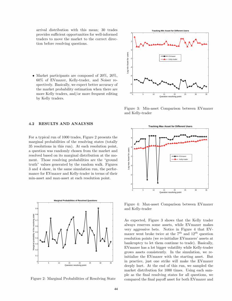
arrival distribution with this mean; 30 tradesprovides sufficient opportunities for well-informedtraders to move the market to the correct direc-tion before resolving questions.

• Market participants are composed of 20%, 20%,60% of EVmaxer, Kelly-trader, and Noiser re-spectively. Basically, we expect better accuracy ofthe market probability estimation when there aremore Kelly traders, and/or more frequent editingby Kelly traders.

4.2 RESULTS AND ANALYSIS

For a typical run of 1000 trades, Figure 2 presents themarginal probabilities of the resolving states (totally35 resolutions in this run). At each resolution point,a question was randomly chosen from the market andresolved based on its marginal distribution at the mo-ment. Those resolving probabilities are the “groundtruth” values generated by the random walk. Figures3 and 4 show, in the same simulation run, the perfor-mance for EVmaxer and Kelly-trader in terms of theirmin-asset and max-asset at each resolution point.

0 5 10 15 20 25 30 350

0.1

0.2

0.3

0.4

0.5

0.6

0.7

0.8

0.9

1Marginal Probabilities of Resolved Questions

Question resolving point

Mar

gina

l pro

babi

lity

of th

e re

solv

ing

stat

e

Figure 2: Marginal Probabilities of Resolving State

0 5 10 15 20 25 30 35-10

-8

-6

-4

-2

0

2

4Tracking Min Asset for Different Users


Log

min

Ass

et fo

r use

rs

EVmaxer

Kelly-trader

Figure 3: Min-asset Comparison between EVmaxerand Kelly-trader

0 5 10 15 20 25 30 35

-4

-2

0

2

4

6

8Tracking Max Asset for Different Users


Log

max

Ass

et fo

r use

rs

EVmaxer

Kelly-trader

Figure 4: Max-asset Comparison between EVmaxerand Kelly-trader

As expected, Figure 3 shows that the Kelly traderalways reserves some assets, while EVmaxer makesvery aggressive bets. Notice in Figure 4 that EV-maxer went broke twice at the 7th and 12th questionresolution points (we re-initialize EVmaxers’ assets atbankruptcy to let them continue to trade). Basically,EVmaxer has a lot bigger volatility while Kelly-tradergrows assets consistently. In the simulation, we re-initialize the EVmaxer with the starting asset. Butin practice, just one strike will make the EVmaxerdeeply hurt. At the end of this run, we sampled themarket distribution for 1000 times. Using each sam-ple as the final resolving states for all questions, wecompared the final payoff asset for both EVmaxer and

44

Kelly-trader. Histograms of the final assets are shownin Figure 5, and 6. As you may notice, Kelly-traderhas very consistent distribution with mean of 58, andstandard deviateion of about 31. But EVmaxer’s finalasset is distributed very sparsely. Most of time (al-most dominant), EVmaxer will have final asset closeto zero, although its possible maximum value can bemore than 1000.

0 50 100 150 200 250 300 350 4000

20

40

60

80

100

120

140

160

180

200Histogram of Final Asset for Kelly-trader

Possible final asset

Freq

uenc

y

Figure 5: Histogram of the final assets for Kelly-trader

0 200 400 600 800 1000 12000

100

200

300

400

500

600

700

800

900

1000Histogram of Final Asset for EVmaxer

Possible final asset

Freq

uenc

y

Figure 6: Histogram of the final assets for EVmaxer

5 TAYLOR APPROXIMATION

In this section, we present an alternate approach inwhich we approximate the utility function by a second-order Taylor series, yielding an approximation to theexpected utility in terms of first and second moments

of the utility random variable. We then apply meth-ods for local computation of moments of real-valuedfunctions defined on graphical models (Nilsson, 2001;Cowell et al., 1999) to obtain an approximation to theexpected utility.

5.1 NOTATION AND DEFINITIONS

Let Zv : v ∈ V be a set of finitely many discreterandom variables; let Ωv denote the set of possiblevalues of Zv, and let zv denote a typical element ofΩv. For C ⊂ V , we write ZC for Zv : v ∈ C, ΩC

for the Cartesian product ×c∈CΩc and zc for a typicalelement of ΩC .

A junction tree T on V is an undirected graph inwhich the nodes are labeled with subsets C ⊂ Vcalled cliques; each arc is labeled with the intersectionS = C ∩D, called the separator, of the cliques at theends of the arc; every v ∈ V is in at least one clique;there is exactly one path between any two cliques, i.e.,T is a tree; and C ∩ D is contained in very cliquealong the path from C to D. We let C denote the setof cliques and S denote the set of separators.

We say a real-valued function f on ΩV factorizes on thejunction tree T if there exist non-negative real-valuedfunctions hC : C ∈ C on ΩC and and hD : D ∈ Don ΩD such that for all v ∈ V :

f(zV ) =

∏C∈C hC(zC)∏D∈D hD(zD)

(6)

where zC and zD denote the components of zV corre-sponding to C and D, respectively, and hD(zD) = 0only if there is at least one clique D with D ∩ C 6= ∅and hC(zC) = 0. In case hD(zD) = 0 and hC(zC) = 0for D ∩ C 6= ∅, we take hC(zC)/hD(zD) to be 0.

We say a function f on ΩV decomposes additively onthe junction tree T if there exist non-negative real-valued functions hC : C ∈ C on ΩC and and hD :D ∈ D on ΩD such that for all v ∈ V :

f(zV ) =∑C∈C

hC(zC)−∑D∈D

hD(zD) (7)

where zC and zD denote the components of zV cor-responding to C and D, respectively. The func-tions hC(xc) and hD(xD) in (6) and (7) are calledpotentials; the set hB : B ∈ C∪D is called a (multi-plicative or additive, respectively) potential represen-tation of f .

45

5.2 ASSETS AND PROBABILITIES

We assume the user’s probability distribution g fac-torizes according to the junction tree T . We assumetrades are constrained to be structure preserving withrespect to T ; hence, the before-trade market distribu-tion p and the market distribution x after a structurepreserving trade also factorize according to T . Con-sequently, as proven in (Sun et al., 2012), the user’scurrent assets a(zV ) decompose additively on T . Fur-ther, if the user makes a structure-preserving trade tochange p to x, the user’s new assets

y(zV ) = a(zV ) + b logx(zV )

p(zV )(8)

decompose additively on T .

The expected assets µY =∑

zVg(zV )y(zV ) can be

computed efficiently by junction tree propagation(Nilsson, 2001).

We assume the user has a logarithmic utility function

u(zV ) = log y(zV ) = log

(a(zV ) + b log

x(zV )

p(zV )

). (9)

We seek to maximize

EU =∑zV

q(zV ) log

(a(zV ) + b log

x(zV )

p(zV )

)(10)

The utility (9) does not decompose additively, and ex-act computation of the expected utility is intractable.However, we can approximate the utility by the first-order Taylor expansion of log y(zV ) around µY as:

u(zV ) ≈ log y(zV ) +(y(zV )− µY )

µY− (y(zV )− µY )2

2µ2Y

.

(11)

We therefore wish to optimize

EU ≈∑zV

log q(zV )

(y(zV )− (y(zV )− µY )2

2µ2Y

)= logµY −

σ2Y

2µ2Y

,

(12)

where σ2Y is the variance of Y . The objective func-

tion (12) can be calculated from the first and secondmoments of Y . Nilsson (2001) showed how to modifythe standard junction tree propagation algorithm to

compute first and second moments of additively de-composable functions efficiently. These results can beapplied to efficient calculation of the approximate ex-pected utility (12), as described below.

5.3 PROPAGATING SECOND MOMENTS

The standard junction tree algorithm (Jensen, 2001;Dawid, 1992; Lauritzen and Spiegelhalter, 1988) oper-ates on a potential representation hB : B ∈ C∪D fora probability distribution g that factorizes on a junc-tion tree T . A clique C is said to be eligible to receivefrom a neighboring clique D if either C is D’s onlyneighbor or D has already received a message from allits neighbors other than C. Any schedule is allowablethat sends messages along arcs only when the recipientis eligible to receive from the sender, and that termi-nates when messages have been sent in both directionsalong all arcs in the junction tree.

Passing a message from D to C has the following effect:

h′S(zS) =∑D\S

hD(zD), and (13)

h′C(zC) = hC(zC)

(h′S(zS)

hS(zS)

)(14)

That is, the new separator potential is obtained bymarginalizing the sender’s potential over the variablesnot contained in the separator, and the new recipientclique potential is obtained by multiplying the old re-cipient potential by the ratio of new to old separatorpotentials.

It is clear that message passing preserves the fac-torization constraint (6). Furthermore, when the al-gorithm terminates, the new clique and separatorpotentials are the marginal distributions gB(zB) =∑

V \B gV (zV ), B ∈ C ∪ S.

Now, suppose in addition to the multiplicative poten-tial representation for g, we have an additive poten-tial representation tB : B ∈ C ∪ S for an addi-tively decomposable function y on ΩV . We modifythe message-passing algorithm to pass a bivariate mes-sage along each arc. Now, in addition to the effects onthe multiplicative potential for the probability distri-bution g, a message from D to C results in the follow-ing change to the additive potential for y:

t′S(zS) =

∑D\S hD(zD)tD(zD)∑

D\S hD(zD), and (15)

t′C(zC) = tC(zC) + t′S(zS)− tS(zS) (16)

46

After the algorithm terminates with messages sent inboth directions along all arcs, the final clique and sep-arator multiplicative potentials contain the associatedmarginal distributions; and the clique and separatoradditive potentials contain the conditional expecta-tion of Y given the clique/separator state µY |B(zB) =∑

V \B gV (zV )yV (zV )/∑

V \B gV (zV ), B ∈ C ∪ S.

After propagation, finding the first moment of Y isstraightforward: we simply marginalize the additivepotential on any clique or separator:

µY =∑B

µY |B(zB) (17)

Recall that after propagation, the multiplicative po-tentials are the marginal probabilities gB(zB) and themultiplicative potentials are the conditional expecta-tions µY |B(zB) for B ∈ C ∪ S. Nilsson (2001) provedthat the second moment of the additively decompos-able function Y can be calculated from the post-propagation additive and multiplicative potentials asfollows:

E[Y 2] =∑C∈C

∑zC

gC(zC)µY |C(zC)2

−∑S∈S

∑zS

gD(zS)µY |S(zS)2.(18)

To see why (18) is correct, note that by definition,E[Y 2] =

∑zug(zu)y(zu)2. Then:

E[Y 2] =∑zu

g(zu)y(zu)2

=∑zu

g(zu)y(zu)

(∑C∈C

µY |C(zC)−∑S∈S

µY |S(zS)µ

)=∑C∈C

∑zu

gu(zu)y(zu)µY |C(zC)

−∑D∈D

∑zu

gu(zu)y(zu)µY |S(zS)

=∑C∈C∑zC

µY |C(zC)∑zU\C

gu(zu)y(zu)

−∑S∈S∑zS

µY |S(zS)∑zU\S

gu(zu)y(zu)

=∑C∈C

∑zC

gC(zC)µY |C(zC)2

−∑S∈S

∑zS

gS(zS)µY |S(zS)2.

For a more accurate approximation, we can add addi-tional terms to the Taylor expansion and apply Cow-

ell’s method (1999, Sec. 6.4.7) for local propagationof higher moments. In general, we need to propagaten+ 1 potentials to compute the first n moments of thedistribution of Y .

6 SUMMARY

By any definition, big data requires learners to con-sider only a portion of the data at a time. The problemis then to fuse the beliefs of these specialized agents.We consider a market to be an effective mechanism forfusing the beliefs of an arbitrary mixture of human ex-perts and machine learners, by allowing each agent toconcentrate on those areas where they can do the mostgood (and therefore earn the most points). However,agents that are good at learning are not necessarilygood at trading. Our contribution is a general formu-lation of an agent which will translate a set of beliefsinto optimal or near-optimal trades on a combinato-rial market that has been represented in factored formsuch as a Bayesian network.

It is known from theory and empirical results in evo-lutionary finance that an informed trader seeking tomaximize her wealth should allocate her assets accord-ing to the Kelly (1956) rule. This rule is very general,and applies even to combinatorial markets. However,it would be intractable to solve on an arbitrary jointstate. We have derived two efficient ways to calculateKelly investments given beliefs specified in a factoredjoint distribution – such as a Bayesian network. Wetested the more conservative rule and found that ithas the desired properties: an exponential wealth in-crease which never goes broke, slightly underperform-ing an EV-maximizer in the short run, but outper-forming it in the long run because the EV-maximizerwill go broke.

Our results mean that we can let experts focus on theirbeliefs in any effective manner, and let an automatedagent convert those beliefs into trades. This abilityhas frequently been requested by participants in theIARPA ACE geopolitical forecasting tournament, andwe expect to offer the feature this autumn in our newScience & Technology market.

As a reminder, we assume we have a current set ofbeliefs from our expert. In practice, we will have tospecify a rate at which expressed beliefs converge tothe market, in the absence of future updates from theexpert, so as not forever to chain our participants withthe ghosts of expired beliefs. In addition, we plan toextend our results for systems using approximate in-ference to update the probability distribution.

47

Acknowledgments

Supported by the Intelligence Advanced ResearchProjects Activity (IARPA) via Department of In-terior National Business Center contract numberD11PC20062. The U.S. Government is authorizedto reproduce and distribute reprints for Governmen-tal purposes notwithstanding any copyright annota-tion thereon. Disclaimer: The views and conclusionscontained herein are those of the authors and shouldnot be interpreted as necessarily representing the offi-cial policies or endorsements, either expressed or im-plied, of IARPA, DoI/NBC, or the U.S. Government.

References

Amir, R., Evstigneev, I. V., Hens, T., and Schenk-Hopp, K. R. (2001). Market selection and survivalof investment strategies. Working Paper 91, Univer-sity of Zurich. Institute for Empirical Research inEconomics.

Barbu, A. and Lay, N. (2011). An introductionto artificial prediction markets for classification.arXiv:1102.1465.

Beinlich, I., Suermondt, G., Chavez, R., and Cooper,G. (1989). The alarm monitoring system: A casestudy with two probabilistic inference techniques forbelief networks. In Proceeding of 2nd European Con-ference on AI and Medicine.

Berea, A., Twardy, C., Laskey, K., Hanson, R., andMaxwell, D. (2013). Daggre: An overview of com-binatorial prediction markets. In Proceedings of theSeventh International Conference on Scalable Un-certainty Management (SUM).

Chen, Y., Fortnow, L., Lambert, N., Pennock, D. M.,and Wortman, J. (2008). Complexity of combinato-rial market makers. In Proceedings of the 9th ACMConference on Electronic Commerce (EC), pages190–199.

Chen, Y. and Pennock, D. M. (2010). Designing mar-kets for prediction. AI Magazine, 31(4):42–52.

Cowell, R. G., Dawid, A. P., Lauritzen, S. L., andSpiegelhalter, D. J. (1999). Probabilistic Networksand Expert Systems. Springer-Verlag, New York.

Dawid, A. P. (1992). Applications of a general prop-agation algorithm for probabilistic expert systems.Statistics and Computing, 2:25–36.

Evstigneev, I. V., Hens, T., and Schenk-Hopp, K. R.(2006). Evolutionary stable stock markets. Eco-nomic Theory, 27(2):449–468.

Hanson, R. (2003). Combinatorial information marketdesign. Information Systems Frontiers, 5(1):107–119.

Jensen, F. V. (2001). Bayesian Networks and DecisionGraphs. Springer-Verlag, Berlin, 2001 edition.

Kelly, J. J. (1956). A new interpretation of informationrate. Bell System Technical Journal, 35:917–926.

Lauritzen, S. and Spiegelhalter, D. (1988). Local com-putations with probabilities on graphical structuresand their applications to expert systems. In Pro-ceedings of the Royal Statistical Society, Series B.,volume 50, pages 157–224.

Lensberg, T. and Schenk-Hoppe, K. R. (2007). Onthe evolution of investment strategies and the kellyrule — a darwinian approach. Review of Finance,11:25–50.

Nilsson, D. (2001). The computation of moments ofdecomposable functions in probabilistic expert sys-tems. In booktitle = ”Proceedings of the 3rd Inter-national Symposium on Adaptive Systems”, pages116–121.

Solomonoff, R. J. (1978). Complexity-based induc-tion systems: Comparisons and convergence theo-rems. IEEE Transactions on Information Theory,IT-24:422–432.

Sun, W., Hanson, R., Laskey, K., and Twardy,C. (2012). Probability and asset updating usingbayesian networks for combinatorial prediction mar-kets. In Proceedings of the 28th Annual Conferenceon Uncertainty in Artificial Intelligence (UAI).

Wachter, A. and Biegler, L. T. (2006). On the imple-mentation of a primal-dual interior point filter linesearch algorithm for large-scale nonlinear program-ming. Mathematical Programming, 106(1):25–57.

48

Predicting Latent Variables with Knowledge and Data: A Case Study in Trauma Care

Barbaros Yet1, William Marsh1, Zane Perkins2, Nigel Tai3, Norman Fenton1

1School of Electronic Engineering and Computer Science, Queen Mary, University of London, London, UK

2Centre for Trauma Sciences, Queen Mary, University of London, London, UK 3Royal London Hospital, London, UK

[email protected]

Abstract. Making a prediction that is useful for decision makers is not the same as building a model that fits data well. One reason for this is that we often need to pre-dict the true state of a variable that is only indirectly observed, using measurements. Such ‘latent’ variables are not present in the data and often get confused with meas-urements. We present a methodology for developing Bayesian network (BN) models that predict and reason with latent variables, using a combination of expert knowledge and available data. The method is illustrated by a case study into the pre-diction of acute traumatic coagulopathy (ATC), a disorder of blood clotting that can cause fatality following traumatic injuries. There are several measurements for ATC and previous models have predicted one of these measurements instead of the state of ATC itself. Our case study illustrates the advantages of models that distinguish between an underlying latent condition and its measurements, and of a continuing dialogue between the modeller and the domain experts as the model is developed us-ing knowledge as well as data.

Keywords: Bayesian Networks, Latent Variables, Knowledge Engineering

This paper is published as an abstract only.

49

A Lightweight Inference Method for Image Classification

John Mark [email protected]

Preeti J. [email protected]

Abstract

We demonstrate a two phase classifica-tion method, first of individual pixels,then of fixed regions of pixels for sceneclassification—the task of assigning posteri-ors that characterize an entire image. Thiscan be realized with a probabilistic graphicalmodel (PGM), without the characteristic seg-mentation and aggregation tasks characteris-tic of visual object recognition. Instead thespatial aspects of the reasoning task are de-termined separately by a segmented partitionof the image that is fixed before feature ex-traction. The partition generates histogramsof pixel classifications treated as virtual evi-dence to the PGM. We implement a samplingmethod to learn the PGM using virtual ev-idence. Tests on a provisional dataset showgood (+70%) classification accuracy amongmost all classes.

1 Introduction

Scene recognition is a field of computer understandingfor classification of scene types by analysis of a visualimage. The techniques employed for scene recognitionare well known, relying on methods for image analysisand automated inference. The fundamental process isto assign probabilities over a defined set of categories—the scene characteristics—based on analysis of the cur-rent visual state. This paper shows the practicabilityof a lightweight approach that avoids much of the com-plexity of object recognition methods, by reducing theproblem to a sequence of empirical machine learningtasks.

The problem we have applied this to is classificationof scene type by analysis of a video stream from amoving platform, specifically from a car. In this pa-per we address aspects of spatial reasoning—clearly

there is also a temporal reasoning aspect, which is notconsidered here. In figurative terms the problem maybe compared with Google’s Streetview R© application.Streetview’s purpose is to tell you what your surround-ings look like by knowing your location. The scenerecognition problem is the opposite: to characterizeyour location from what your surroundings look like.

In this paper we consider a classification scheme forimages where the image is subject to classification inmultiple categories. We will consider outdoor roadwayscenes, and these classification categories:

1. surroundings, zoning, development (urban, resi-dential, commercial, mountainous, etc.)

2. visibility (e.g., illumination and weather),

3. roadway type,

4. traffic and other transient conditions,

5. roadway driving obstacles.

An image will be assigned one label from each of theset of five categories.

1.1 Uses of Scene Classification

There are numerous uses where the automated classi-fication assigned to a scene can help. The purpose ofscene classification is to capture the gist of the currentview from its assigned category labels. For example,how would you describe a place from what you see?Certainly this is different from what you would knowfrom just the knowledge of your lat-long coordinates.These are some envisioned uses:

• A scene classification provides context. For ex-ample in making a recommendation, the contextcould be to consider the practicality of the re-quest: For instance, “Do you want to get a lattenow? This is not the kind of neighborhood forthat.”

50

• Supplement search by the local surroundings. Forexample, “Find me a winery in a built-up area.”“Find me a restaurant in a remote place.” “Finda park in a less-travelled residential area.”

• Coming up with a score for the current conditions.How is the view from this place? How shaded orsunny is the area? What fraction of the surround-ings are natural versus artificial? Taking this onestep further, given an individual driver’s ratings ofpreferred locations, suggest other desirable routesto take, possibly out of the way from a “best”route.

• Distributed systems could crowd-source theirfindings about nearby locations to form a com-prehensive picture of an area. For example, “Howfar does this swarm (road-race, parade) extend?”

1.2 Relevant previous work

One of the earliest formulations of image understand-ing as a PGM is found in Levitt, Agosta, and Binford(1989) and Agosta (1990). The approach assumedan inference hierarchy from object categories to low-level image features, and proposed aggregation opera-tors that melded top-down (predictive) with bottom-up (diagnostic) reasoning over the hierarchy.

The uses of PGMs in computer vision have expandedinto a vast range of applications. Just to mention acouple of examples, L. Fei-Fei, Fergus and P. Perona(2003) developed a Bayesian model for learning newobject categories using a “constellation” model withterms for different object parts. In a paper that im-proved upon this, L. Fei-Fei and P. Perona (2005)proposed a Bayesian hierarchical theme model thatautomatically recognizes natural scene categories suchas forest, mountains, highway, etc. based on a gen-eralization of the original texton model by T. Leungand J. Malik (2001) and, L. Fei-Fei R. VanRullen, C.Koch, and P. Perona (2002). In another applicationof a Bayesian model, Sidenbladh, Black, and Fleet(2000) develop a generative model for the appearanceof human figures. Both of these examples apply modelselection methods to what are implicitly PGMs, if notexplicitly labeled as such.

Computer vision approaches specifically to scenerecognition recognize the need to analyze the image asa whole. Hoiem, Efros, and Hebert (2008) approachthe problem by combining results from a set of in-trinsic images, each a map of the entire image for oneaspect of the scene. Oliva and Torralba (2006) developa set of scene-centered global image features that cap-ture the spatial layout properties of the image. Sim-ilar to our approach, their method does not requiresegmentation or grouping steps.

1.3 How Scene Classification differs fromObject Recognition

Scene classification implies a holistic image-level in-ference task as opposed to the task of recovering theidentity, presence, and pose of objects within an im-age. Central to object recognition is to distinguishthe object from background of the rest of the image.Typically this is done by segmenting the image into re-gions of smoothly varying values separated by abruptboundaries, using a bottoms-up process. Pixels maybe grouped into “super-pixels” whose grouping is fur-ther refined into regions that are distinguished as partof the foreground or background. Object recognitionthen considers the features and relationships amongforeground regions to associate them with parts to beassembled into the object, or directly with an entireobject to be recovered.

Scene classification as we approach it does not neces-sarily depend on segmenting the image into regions,or identifying parts of the image. Rather it achievesa computational economy by treating the image as awhole; for example, to assign the image to the classof “indoor,” “outdoor,” “urban landscape,” or “rurallandscape,” etc. from a set of pre-defined categories.We view classification as assigning a posterior to classlabels, where the image may be assigned a value overmultiple sets of labels; equivalently, the posterior maybe a joint distribution over several scene variables.

Despite the lack of a bottoms-up segmentation step inour approach, our method distinguishes regions of theimage by a partition that is prior to analyzing the im-age contents. This could be a fixed partition, whichis appropriate for a camera in a fixed location such asa security camera, or it could depend on inferring thegeometry of the location from sources distinct fromthe image contents, such as indicators of altitude andazimuth of the camera. In our case, the prior pre-sumption is that the camera is on the vehicle, facingforward, looking at a road.

The rest of this paper is organized as follows. Section 2describes the inference procedure cascade; the specificdesign and learning of the Bayes network PGM is thesubject of Section 3, and the results of the learnedmodel applied to classification of a set of images ispresented in Section 4.

2 Lightweight inference with virtualevidence

In treating the image as a whole, our approach to infer-ence for scene classification takes place by a sequenceof two classification steps:

51

• First the image’s individual pixels are classified,based on pixel level features. This classifier re-solves the pixel into one of n discrete types, rep-resenting the kind of surface that generated it.In our examples n = 8: sky, foliage, building-structure, road-surface, lane, barrier-sidewalk, ve-hicle, and pedestrian.

• In the second step, the pre-defined partitions areapplied to the image and in each partition thepixel types are histogrammed, to generate a like-lihood vector for the partition. These likelihoodsare interpreted as virtual evidence1 for the secondlevel image classifier, the scene classifier, imple-mented as a PGM. The classifier returns an jointdistribution over the scene variables, inferred fromthe partitions’ virtual evidence.

There is labeled data for both steps, to be able to learna supervised classifier for each. Each training image ismarked up into labeled regions using the open sourceLabelMe tool, (Russell, Torralba, K. Murphy and Free-man, 2007) and also labeled by one label from eachcategory of scene characteristics. From the region la-belings a dataset of pixels, with color and texture asfeatures, and the region they belong to as labels canbe created. In the second step we learn the structureand parameters of a Bayes network—a discrete valuedPGM—from the set of training images that have beenmanually labeled with scene characteristics. Each im-age has one label assigned for each scene characteristic.The training images are reduced to a set of histogramsof the predicted labels for the pixels, one for each par-tition. The supervised data for an image consists ofthe histogram distributions and the label set.

Scene recognition output is a summarization of a visualinput as an admittedly modest amount of informationfrom a input source orders of magnitude greater–evenmores than for the object recognition task. From theorder of 106 pixel values we infer a probability distri-bution over a small number of discrete scene classifi-cation variables. To obtain computational efficiency,we’ve devised an approach that summarizes the infor-mation content of the image in an early stage of theprocess that is adequate at later stages for the classi-fication task.

2.1 Inference Cascade

The two phases in the inference cascade can be for-malized as follows, starting from the pixel image and

1Sometimes called “soft evidence.” We prefer the termvirtual evidence, since soft evidence is also used to mean anapplication of Jeffrey’s rule of conditioning that can changethe CPTs in the network.

resulting in a probability distribution over scene char-acteristics. Consider an image of pixels pij over i× j,each pixel described by a vector of features fij . Thefeatures are derived by a set of filters, e.g. for colorand texture, centered at coordinate (i, j). A pixel-levelclassifier is a function from the domain of f to one ofa discrete set of n types, C : f → c(1), · · · c(n). Theresult is an array of classified image pixels.

A pre-determined segmentation, Gm partitions thepixels in the image into M regions by assign-ing each pixel to one region, rm = pij | pij ∈Gm,m = 1 . . .M , to form regions that are con-tiguous sets of pixels. Each region is describedby a histogram of the pixel types it contains:Hm =

(|C(fij) = c(1)|, · · · |C(fij) = c(n)|

)s.t. fij ∈

Gm, for which we introduce the notation, Hm =(|c(1)

ij |m, · · · |c(n)ij |m

), where |c(i)|m denotes the count

of pixels of type c(i) in region m. The scene classi-fier is a PGM with virtual evidence nodes correspond-ing to the M regions of the image. See Figure 3.Each evidence node receives virtual evidence in theform of a lambda message, λm, with likelihoods in theratios given by Hm. The PGM model has a subsetof nodes S = S1, · · ·Sv, distinct from its evidencenodes, for scene characteristic variables, each with adiscrete state space. Scene classification is completelydescribed by P(S |λ1, · · ·λM ), the joint of S when theλm are applied, or by a characterization of the jointby the MAP configuration over S, or just the posteriormarginals of S.

2.2 Partitions of Pixel-level Data

As mentioned we avoid segmenting the image basedon pixel values by using a fixed partition to groupclassified pixels. We introduce a significant simplifi-cation over conventional object recognition methodsby using such a segmentation. This makes sense be-cause we are not interested in identifying things thatare in the image, but only in treating the image as awhole. For instance in the example we present here,the assumption is that the system is classifying an out-door roadway scene, with sky above, road below, andsurroundings characteristic of the scene to either side.The partitions approximate this division. The image ispartitioned symmetrically into a set of twelve wedges,formed by rays emanating from the image center.

For greater efficiency the same method could be ap-plied over a smoothed, or down-sampled image, so thatevery pixel need not be touched, only pixels on a reg-ular grid. The result of the classification step is a dis-crete class-valued image array. See Figure 2. Despitethe classifier ignoring local dependencies, neighboringpixels tend to be classed similarly, and the class-valued

52

image resembles a cartoon version of the original.

Figure 1: The original image. The barriers borderingthe lane are a crucial feature that the system is trainedto recognize.

Figure 2: The image array of C(fij), the pixel classi-fier, on an image down-sampled to 96 by 54. Rays em-anating from the image center show the wedge-shapedregions. Colors are suggestive of the pixel class, e.g.green indicates foliage and beige indicates barriers.

2.2.1 Inferring partition geometry

The point chosen as the image center, where the ver-tices of the wedges converge approximates the vanish-ing point of the image. Objects in the roadway scenetend to conform (very) roughly to the wedge outlinesso that their contents are more uniform, and hence,likelihoods are more informative. For example, thecontents of the image along the horizon will fall withinone wedge, and the road surface within another.

2.3 The image as a source of virtual evidence

For each wedge that partitions the image, the evidenceapplied to the Bayes network from the wedge m is:λm ∝ |c(1)

ij |m : |c(2)ij |m : · · · : |c(n)

ij |m. One typicallythinks of virtual evidence as a consequence of mea-surements coming from a sensor that garbles the pre-

cise value of the quantity of interest—where the actualobserved evidence value is obscured by an inaccuracyin the sensor reading. Semantically, one should notthink of the virtual image evidence as a garbled sensorvariable. Rather it is the evidence that describes theregion.

3 Bayes network design

Formally a Bayes network is a factorization of a jointprobability distribution into local probability mod-els, each corresponding to one node in the network,with directed arcs between the nodes showing theconditioning of one node’s probability model on an-other’s (Koller and Friedman, 2010). Inference—for example, classification—operates in the directionagainst the causal direction of the arc. In short, in-ference flows from lower level evidence in the networkupward to the class nodes at the top of the networkwhere it generates the posterior distributions over theclass variables, in this case, the scene characteristics.We learn a fully observable Bayes network with virtualevidence for scene classification.

3.1 How the structure and parameters aredefined

The design of the Bayes network model is fluid: It iseasily re-learned under different partition inputs, out-put categories and structural constraints. The abilityto easily modify the model to test different kinds ofevidence as inputs, or differently defined nodes as out-puts is an advantage of this approach. The structureof the model discovers dependencies among the modelvariables that reveal properties of the domain.

Learning the Bayes network is composed of two as-pects; the first, learning the variables’ structure, thesecond, learning the parameters of the variable con-ditional probability tables. The algorithm used isSMILE’s Bayesian Search (Druzdzel et al., 1997), aconventional fully observable learning algorithm, witha Bayesian scoring rule used to select the preferredmodel. Learning structure and parameters occur si-multaneously.

The model is structured into two levels, the top level ofoutputs and the lower level of inputs as shown in Fig-ure 3. This is the canonical structure for classificationwith a Bayes network, in this case a multi-classifierwith multiple output nodes. In the learning procedurethis node ordering is imposed as a constraint on thestructure, so that conditioning arcs cannot go from thelower level to the upper level.

Further constraints are used to limit in-degree andnode ordering. The in-degree of evidence nodes is

53

limited to two. Node ordering of output nodes fol-lows common sense causal reasoning: for instance, the“Surroundings” variable influences the “Driving Con-ditions” and not the other way around. The modelconsequently follows an approximately naive Bayesstructure for each scene variable, but with additionalarcs that are a consequence of the model selection per-formed during learning. The resulting network is rela-tively sparse and hence learning a network of this size,let alone running inference on it can be done interac-tively.

3.2 Bayes Network Learning Dataset

An interesting challenge in learning this model is thatthere is no conventional procedure for learning fromvirtual evidence, such as the histogram data.

3.2.1 Consideration of partition contents asvirtual evidence

We considered three ways to approximate learning theBayes network from samples that include virtual evi-dence.

1) Convert the dataset into an approximate equiva-lent observed evidence dataset by generating multi-ples of each evidence row, in proportion to the likeli-hood fraction for each state of the virtual evidence. Ifthere are multiple virtual evidence nodes, then to cap-ture dependencies among virtual evidence nodes thiscould result in a combinatorial explosion of row sets,one multiple for each combination of virtual evidencenode states, with multiplicities in proportion to thelikelihood of the state combination. This is equivalentin complexity to combining all virtual evidence nodesinto one node for sampling.

Similarly one could sample from the combination of allvirtual evidence nodes and generate a sample of rowsbased on the items in the sample. This is a bit likelogic sampling the virtual states.

Both these methods make multiple copies of a row inthe learning set as a way to emulate a training weight.Instead one could apply a weight to each row in thesampled training set, in proportion to its likelihood.

2) One could also consider a mixture, a “multi-net,”of learned deterministic evidence models. The mod-els would have the same structure, so the result wouldbe a mixture of CPTs, weighted (in some way) by thelikelihoods. It appears this would also suffer a combi-natorial explosion of mixture components, and mightbe amenable to reducing the set by sampling.

3) Alternatively, one could consider the virtual evi-dence by a virtual node that gets added as a child

to the evidence node, which is then instantiated tosend the equivalent lambda msg to its parent. This isthe method used in Refaat, Choi and Darwiche (2012).With many cases, there would be a set of virtual nodesadded to the network for each case, again generatinga possibly unmanageable method. Perhaps there is anincremental learning method that would apply: Builda network with one set of nodes, do one learning step,then replace the nodes with the next set, and repeat alearning step.

4 Results on a sample dataset

In this section we present the evaluation of the Bayesnetwork as a classifier. We argue that the first-stagepixel-level classifier, whose accuracy approaches 90%,is a minor factor in the scene classification results,since the partition-level inputs to the Bayes networkaverage over a large number of pixels, although thispremise could be tested.

4.1 Learning from a sampled dataset

The sample dataset to learn the model was a furtherapproximation on alternative 1), where each virtualevidence node was sampled independently to convertthe problem into an equivalent one with sampled data.Each histogram was sampled according to its likeli-hood distribution, to generate a set of conventionalevidence samples that approximated the histogram.The result was an expanded dataset that multipliedthe number rows by the sample size for each row inthe histogram dataset. The resulting dataset descrip-tion is:

1. Original data set: 122 rows of 12 region his-tograms of images labeled by 5 scene labels.

2. Each region histogram is sampled 10 times, togenerate 1220 rows

3. Final data set of 5 labels and 12 features by 1220rows

4.2 Inference Results

As mentioned, the second-stage Bayes network classi-fier infers a joint probability distribution over the setof scene characteristic nodes—the nodes shown in or-ange in Figure 3. We will evaluate the scene classifierby the accuracy of the predicted marginals, comparingthe highest posterior prediction for each scene variablewith the true value.2

2The “dynamic environment” variable is not countedin the evaluation results, since most all labeled data wascollected under overcast conditions, making the predictedresults almost always correct, and uninteresting.

54

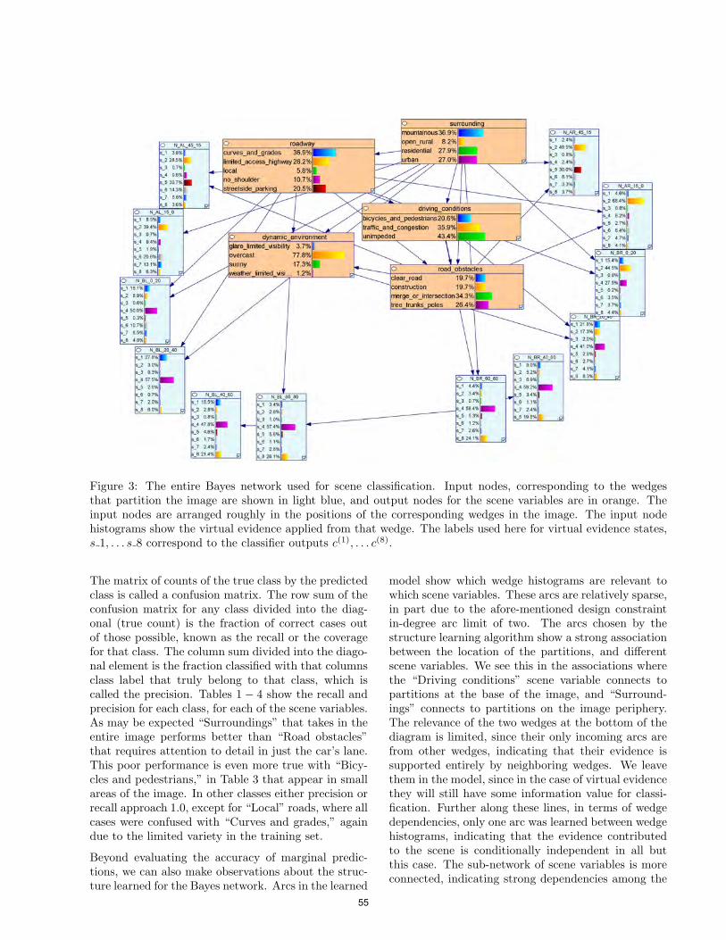
Figure 3: The entire Bayes network used for scene classification. Input nodes, corresponding to the wedgesthat partition the image are shown in light blue, and output nodes for the scene variables are in orange. Theinput nodes are arranged roughly in the positions of the corresponding wedges in the image. The input nodehistograms show the virtual evidence applied from that wedge. The labels used here for virtual evidence states,s 1, . . . s 8 correspond to the classifier outputs c(1), . . . c(8).

The matrix of counts of the true class by the predictedclass is called a confusion matrix. The row sum of theconfusion matrix for any class divided into the diag-onal (true count) is the fraction of correct cases outof those possible, known as the recall or the coveragefor that class. The column sum divided into the diago-nal element is the fraction classified with that columnsclass label that truly belong to that class, which iscalled the precision. Tables 1− 4 show the recall andprecision for each class, for each of the scene variables.As may be expected “Surroundings” that takes in theentire image performs better than “Road obstacles”that requires attention to detail in just the car’s lane.This poor performance is even more true with “Bicy-cles and pedestrians,” in Table 3 that appear in smallareas of the image. In other classes either precision orrecall approach 1.0, except for “Local” roads, where allcases were confused with “Curves and grades,” againdue to the limited variety in the training set.

Beyond evaluating the accuracy of marginal predic-tions, we can also make observations about the struc-ture learned for the Bayes network. Arcs in the learned

model show which wedge histograms are relevant towhich scene variables. These arcs are relatively sparse,in part due to the afore-mentioned design constraintin-degree arc limit of two. The arcs chosen by thestructure learning algorithm show a strong associationbetween the location of the partitions, and differentscene variables. We see this in the associations wherethe “Driving conditions” scene variable connects topartitions at the base of the image, and “Surround-ings” connects to partitions on the image periphery.The relevance of the two wedges at the bottom of thediagram is limited, since their only incoming arcs arefrom other wedges, indicating that their evidence issupported entirely by neighboring wedges. We leavethem in the model, since in the case of virtual evidencethey will still have some information value for classi-fication. Further along these lines, in terms of wedgedependencies, only one arc was learned between wedgehistograms, indicating that the evidence contributedto the scene is conditionally independent in all butthis case. The sub-network of scene variables is moreconnected, indicating strong dependencies among the

55

scene variables. Some of these are to be expected, forinstance “Curves and grades” correlates strongly with“Mountainous” surroundings. Some are spurious, asa result of biased selection of the training sample im-ages, (e.g. all divided highway images correspondedto overcast scenes) and have been corrected by addingmore samples.

4.3 Discussion and Conclusion

We have demonstrated a novel scene classification al-gorithm that takes advantage of the presumed geom-etry of the scene to avoid computationally expensiveimage processing steps characteristic of object recogni-tion methods, such as pixel segmentation, by a cascadeof a pixel level and fixed partition level multi-classifier,for which we learn a Bayes network. As a consequenceof the partition-level data we learn the Bayes networkwith virtual evidence.

The Bayes network classifies the scene in several de-pendent dimensions corresponding to a set of cate-gories over which a joint posterior of scene character-istics is generated. Here we have only considered themarginals over categories, however it is a valid ques-tion whether a MAP interpretation—of the most likelycombination of labels—is more appropriate.

The use of virtual evidence also raises questions aboutwhether it is proper to consider the virtual evidencelikelihood as a convex combination of “pure” imagedata. Another interpretation is that the histogramswe are using are better“sliced and diced” to generatestrong evidence from certain ratios of partition con-tent. For instance a partition that includes a smallfraction of evidence of roadway obstacles—think evi-dence of a small person—may be a larger concern thana partition obviously full of obstacles, and should notbe considered a weaker version of the extreme parti-tion contents. These subtleties could be consideredas we expand the applicability of the system. In thisearly work it suffices that given the approximations,useful and accurate results can be achieved at modestcomputational cost.

Acknowledgements

This work would not have been possible without valu-able discussions with Ken Oguchi and Joseph Dugash,and by Naiwala Chandrasiri, Saurabh Barv, GaneshYalla, and Yiwen Wan.

References

Agosta, J. M., 1990. The structure of Bayes networks forvisual recognition, UAI (1988) North-Holland Publish-ing Co., pp. 397 - 406.

Druzdzel, M. et. al., 1997. SMILE (StructuralModeling, Inference, and Learning Engine)http://genie.sis.pitt.edu/.

Fei-Fei, L., R. Fergus, P. Perona, 2003. A Bayesian Ap-proach to Unsupervised One-Shot Learning of ObjectCategories (ICCV 2003), pp. 1134-1141 vol.2.

Fei-Fei L. and P. Perona, 2005. A Bayesian HierarchicalModel for Learning Natural Scene Categories. (CVPR2005), pp. 524-531.

Fei-Fei, L., R. VanRullen, C. Koch, and P. Perona, 2002.Natural scene categorization in the near absence of at-tention(PNAS 2002), 99(14):95969601.

Hoiem, D., A. A. Efros, and M. Hebert. 2008. Closing theLoop in Scene Interpretation.2008 IEEE Conference onComputer Vision and Pattern Recognition (June): 18.

Koller, D., and Friedman, N. 2010. Probabilistic GraphicalModels: Principles and Techniques. Cambridge, Mas-sachusetts: The MIT Press.

Leung, T. and J. Malik, 2001. Representing and recog-nizing the visual appearance of materials using three-dimensional textons(IJCV 2001), 43(1):2944.

Levitt, T., J. M. Agosta, T.O. Binford, 1989. Model-basedinfluence diagrams for machine vision, (UAI 1989).

Oliva, A., and A. Torralba. 2006. Building the Gist of aScene: The Role of Global Image Features in Recogni-tion.Progress in Brain Research 155 (January): 2336.

Oliva, A., A. Torralba, 2001. Modeling the shape of thescene: a holistic representation of the spatial envelope.International Journal of Computer Vision, Vol. 42(3):145-175.

Refaat, K. S. , A. Choi and A. Darwiche, 2012. New Ad-vances and Theoretical Insights into EDML. (UAI 2012),pp. 705-714 .

Russell, B., A. Torralba, K. Murphy, W. T. Freeman, 2007.“LabelMe: a database and web-based tool for image an-notation” International Journal of Computer Vision.

Sidenbladh, H., M. J. Black, and D. J. Fleet, 2000. Stochas-tic Tracking of 3D Human Figures Using 2D Image Mo-tion. ECCV 2000: 702718.

56

MountainousOpenrural Residential Urban

Recall 1.0 0.9 0.794 0.45Precision 0.642 1.0 0.964 1.0Accuracy 0.784

Table 1: Surroundings

Curvesand

grades

Limitedaccess

highwayLocal

Noshoulder

Streetsideparking

Recall 1.0 0.75 0.0 0.85 0.56Precision 0.61 1.0 NaN 1.0 1.0Accuracy 0.770

Table 2: Roadways

Bicycles andpedestrians

Traffic andcongestion Unimpeded

Recall 0.56 0.6 0.98Precision 0.875 0.93 0.67Accuracy 0.754

Table 3: Driving Conditions

Clear road ConstructionMerge

intersection

Treetrunks

and polesRecall 0.42 0.96 0.6 1.0Precision 1.0 0.92 0.86 0.55Accuracy 0.738

Table 4: Road Obstacles

57

Product Trees for Gaussian Process Covariance in Sublinear Time

David A. MooreComputer Science Division

University of California, BerkeleyBerkeley, CA 94709

[email protected]

Stuart RussellComputer Science Division

University of California, BerkeleyBerkeley, CA 94709

[email protected]

Abstract

Gaussian process (GP) regression is a pow-erful technique for nonparametric regression;unfortunately, calculating the predictive vari-ance in a standard GP model requires timeO(n2) in the size of the training set. Thisis cost prohibitive when GP likelihood cal-culations must be done in the inner loop ofthe inference procedure for a larger model(e.g., MCMC). Previous work by Shen et al.(2006) used a k-d tree structure to approxi-mate the predictive mean in certain GP mod-els. We extend this approach to achieve effi-cient approximation of the predictive covari-ance using a tree clustering on pairs of train-ing points. We show empirically that this sig-nificantly increases performance at minimalcost in accuracy. Additionally, we apply ourmethod to “primal/dual” models having bothparametric and nonparametric componentsand show that this enables efficient computa-tions even while modeling longer-scale varia-tion.

1 Introduction

Complex Bayesian models often tie together manysmaller components, each of which must provide itsoutput in terms of probabilities rather than discretepredictions. As a natively probabilistic technique,Gaussian process (GP) regression (Rasmussen andWilliams, 2006) is a natural fit for such systems, butits applications in large-scale Bayesian models havebeen limited by computational concerns: training aGP model on n points requires O(n3) time, while com-puting the predictive distribution at a test point re-quires O(n) and O(n2) operations for the mean andvariance respectively.

This work focuses specifically on the fast evaluation of

GP likelihoods, motivated by the desire for efficient in-ference in models that include a GP regression compo-nent. In particular, we focus on the predictive covari-ance, since this computation time generally dominatesthat of the predictive mean. In our setting, trainingtime is a secondary concern: the model can always betrained offline, but the likelihood evaluation occurs inthe inner loop of an ongoing inference procedure, andmust be efficient if inference is to be feasible.

One approach to speeding up GP regression, com-mon especially to spatial applications, is the use ofcovariance kernels with short lengthscales to inducesparsity or near-sparsity in the kernel matrix. Thiscan be exploited directly using sparse linear algebrapackages (Vanhatalo and Vehtari, 2008) or by morestructured techniques such as space-partitioning trees(Shen et al., 2006; Gray, 2004); the latter approachescreate a query-dependent clustering to avoid consid-ering regions of the data not relevant to a particularquery. However, previous work has focused on effi-cient calculation of the predictive mean, rather thanthe variance, and the restriction to short lengthscalesalso inhibits application to data that contain longer-scale variations.

In this paper, we develop a tree-based method toefficiently compute the predictive covariance in GPmodels. Our work extends the weighted sum algo-rithm of Shen et al. (2006), which computes the pre-dictive mean. Instead of clustering points with sim-ilar weights, we cluster pairs of points having simi-lar weights, where the weights are given by a kernel-dependent distance metric defined on the product spaceconsisting of all pairs of training points. We show howto efficiently build and compute using a product treeconstructed in this space, yielding an adaptive covari-ance computation that exploits the geometric struc-ture of the training data to avoid the need to explicitlyconsider each pair of training points. This enables usto present what is to our knowledge the first account ofGP regression in which the major test-time operations

58

(predictive mean, covariance, and likelihood) run intime sublinear in the training set size, given a suitablysparse kernel matrix. As an extension, we show howour approach can be applied to GP models that com-bine both parametric and nonparametric components,and argue that such models present a promising optionfor modeling global-scale structure while maintainingthe efficiency of short-lengthscale GPs. Finally, wepresent empirical results that demonstrate significantspeedups on synthetic data as well as a real-world seis-mic dataset.

2 Background

2.1 GP Regression Model

We assume as training input a set of labeled points(xi, yi)|i = 1, . . . , n, where we suppose that

yi = f(xi) + εi

for some unknown function f(·) and i.i.d. Gaussian ob-servation noise εi ∼ N (0, σ2

n). Treating the estimationof f(·) as a Bayesian inference problem, we considera Gaussian process prior distribution f(·) ∼ GP (0, k),parameterized by a positive-definite covariance or ker-nel function k(x, x′). Given a set X∗ containing mtest points, we derive a Gaussian posterior distribu-tion f(X∗) ∼ N (µ∗,Σ∗), where

µ∗ = K∗TK−1y y (1)

Σ∗ = K∗∗ −K∗TK−1y K∗ (2)

and Ky = K(X,X) + σ2nI is the covariance matrix of

training set observations, K∗ = k(X,X∗) denotes then×m matrix containing the kernel evaluated at eachpair of training and test points, and similarly K∗∗ =k(X∗, X∗) gives the kernel evaluations at each pairof test points. Details of the derivations, along withgeneral background on GP regression, can be found inRasmussen and Williams (2006).

In this work, we make the additional assumption thatthe input points xi and test points x∗p lie in some met-ric space (M, d), and that the kernel is a monotoni-cally decreasing function of the distance metric. Manycommon kernels fit into this framework, including theexponential, squared-exponential, rational quadratic,and Matern kernel families; anisotropic kernels can berepresented through choice of an appropriate metric.

2.2 k-d and Metric Trees

Tree structures such as k-d trees (Friedman et al.,1977) form a hierarchical, multiresolution partition-ing of a dataset, and are commonly used in machinelearning for efficient nearest-neighbor queries. They

Figure 1: Cover tree decomposition of seismic eventlocations recorded at Fitzroy Crossing, Australia (withX marking the station location).

have also been adapted to speed up nonparametric re-gression (Moore et al., 1997; Shen et al., 2006); thegeneral approach is to view the regression computa-tion of interest as a sum over some quantity associ-ated with each training point, weighted by the kernelevaluation against a test point. If there are sets oftraining points having similar weight – for example,if the kernel is very wide, if the points are very closeto each other, or if the points are all far enough fromthe query to have effectively zero weight – then theweighted sum over the set of points can be approxi-mated by an unweighted sum (which does not dependon the query and may be precomputed) times an es-timate of the typical weight for the group, saving theeffort of examining each point individually. This isimplemented as a recursion over a tree structure aug-mented at each node with the unweighted sum over alldescendants, so that recursion can be cut off with anapproximation whenever the weight function is shownto be suitably uniform over the current region.

Major drawbacks of k-d trees include poor perfor-mance in high dimensions and a limitation to Eu-clidean spaces. By contrast, we are interested in non-Euclidean metrics both as a matter of practical appli-cation (e.g., in a geophysical setting we might considerpoints on the surface of the earth) and because somechoices of kernel function require our algorithm to op-erate under a non-Euclidean metric even if the under-lying space is Euclidean (see section 3.2). We thereforeconsider instead the class of trees having the followingproperties: (a) each node n is associated with somepoint xn ∈M, such that all descendants of n are con-tained within a ball of radius rn centered at xn, and(b) for each leaf L we have xL ∈ X, with exactly oneleaf node for each training point xi ∈ X. We call anytree satisfying these properties a metric tree.

59

function WeightedMetricSum(node n, query points (x∗i , x∗

j ),

. accumulated sum S, tolerances εrel, εabs)δn ← δ((x∗

i ,x∗j ), (n1,n2))

if n is a leaf then

S ← S + (K−1y )n ·

(k(d(x∗

i ,n1)) · k(d(x∗j ,n2))

)else

wmin ← kprodlower (δn + rn)

wmax ← kprodupper (max(δn − rn, 0))

if wmax · SAbsn ≤

(εrel

∣∣∣S + wmin · SUWn

∣∣∣+ εabs

)then

S ← S + 12 (wmax + wmin) · SUW

nelse

for each child c of nsorted by ascending δ((x∗

i ,x∗j ), (c1, c2)) do

S ← S + WeightedMetricSum(c, (x∗i ,x

∗j ), S, εrel, εabs)

end forend if

end ifreturn S

end function

Figure 2: Recursive algorithm to computing GP co-variance entries using a product tree. Abusing nota-tion, we use n to represent both a tree node and thepair of points n = (n1,n2) associated with that node.

Examples of metric trees include many structures de-signed specifically for nearest-neighbor queries, such asball trees (Uhlmann, 1991) and cover trees (Beygelz-imer et al., 2006), but in principle any hierarchicalclustering of the dataset, e.g., an agglomerative clus-tering, might be augmented with radius information tocreate a metric tree. Although our algorithms can op-erate on any metric tree structure, we use cover treesin our implementation and experiments. A cover treeon n points can be constructed in O(n log n) time, andthe construction and query times scale only with theintrinsic dimensionality of the data, allowing for ef-ficient nearest-neighbor queries in higher-dimensionalspaces (Beygelzimer et al., 2006). Figure 1 shows acover-tree decomposition of one of our test datasets.

3 Efficient Covariance using ProductTrees

We consider efficient calculation of the GP covari-ance (2). The primary challenge is the multiplicationK∗TK−1y K∗. For simplicity of exposition, we will fo-cus on computing the (i, j)th entry of the resultingmatrix, i.e., on the multiplication k∗i

TK−1y k∗j wherek∗i denotes the vector of kernel evaluations betweenthe training set and the ith test point, or equivalentlythe ith column of K∗. Note that a naıve implementa-tion of this multiplication requires O(n2) time.

We might be tempted to apply the vector multiplica-tion primitive of Shen et al. (2006) separately for eachrow of K−1y to compute K−1y k∗j , and then once moreto multiply the resulting vector by k∗i . Unfortunately,this requires n vector multiplications and thus scales(at least) linearly in the size of the training set. In-

stead, we note that we can rewrite k∗iTK−1y k∗j as a

weighted sum of the entries of K−1y , where the weightof the (p, q)th entry is given by k(x∗i ,xp)k(x∗j ,xq):

k∗iTK−1y k∗j =

n∑p=1

n∑q=1

(K−1y )pqk(x∗i ,xp)k(x∗j ,xq). (3)

Our goal is to compute this weighted sum efficientlyusing a tree structure, similar to Shen et al. (2006),except that instead of clustering points with similarweights, we now want to cluster pairs of points havingsimilar weights.

To do this, we consider the product spaceM×M con-sisting of all pairs of points fromM, and define a prod-uct metric δ on this space. The details of the productmetric will depend on the choice of kernel function, asdiscussed in section 3.2 below. For the moment, we willassume a SE kernel, of the form kSE(d) = exp(−d2),for which a natural choice is the 2-product metric:

δ((xa,xb), (xc,xd)) =√d(xa,xc)2 + d(xb,xd)2.

Note that this metric, taken together with the SE ker-nel, has the fortunate property

kSE(d(xa,xb))kSE(d(xc,xd)) = kSE(δ((xa,xb), (xc,xd))),

i.e., the property that evaluating the kernel in theproduct space (rhs) gives us the correct weight for ourweighted sum (3) (lhs).

Now we can run any metric tree construction algo-rithm (e.g., a cover tree) using the product metric tobuild a product tree on all pairs of training points. Inprinciple, this tree contains n2 leaves, one for each pairof training points. In practice it can often be mademuch smaller; see section 3.1 for details. At each leafnode L, representing a pair of training points, we storethe element (K−1y )L corresponding to those two train-ing points, and at each higher-level node n we cachethe unweighted sum SUWn of these entries over all ofits descendant leaf nodes, as well as the sum of abso-lute values SAbsn (these cached sums will be used todetermine when to cut off recursive calculations):

SUWn =

∑L∈leaves(n)

(K−1y )L (4)

SAbsn =

∑L∈leaves(n)

∣∣(K−1y )L∣∣ . (5)

Given a product tree augmented in this way, theweighted-sum calculation (3) is performed by theWeightedMetricSum algorithm of Figure 2. Thisalgorithm is similar to the WeightedSum andWeightedXtXBelow algorithms of Shen et al.(2006) and Moore et al. (1997) respectively, but

60

adapted to the non-Euclidean and non-binary tree set-ting, and further adapted to make use of bounds on theproduct kernel (see section 3.2). It proceeds by a recur-sive descent down the tree, where at each non-leaf nodeit computes upper and lower bounds on the weight ofany descendant, and applies a cutoff rule to determinewhether to continue the descent. Many cutoff rules arepossible; for predictive mean calculation, Moore et al.(1997) and Shen et al. (2006) maintain an accumulatedlower bound on the total overall weight, and cut offwhenever the difference between the upper and lowerweight bounds at the current node is a small fractionof the lower bound on the overall weight. However, oursetting differs from theirs: since we are computing aweighted sum over entries of K−1y , which we expect tobe approximately sparse, we expect that some entrieswill contribute much more than others. Thus we wantour cutoff rule to account for the weights of the sumand the entries of K−1y that are being summed over.We do this by defining a rule in terms of the currentrunning weighted sum,

wmax · SAbsn ≤

(εrel

∣∣∣S + wmin · SUWn

∣∣∣+ εabs

), (6)

which we have found to significantly improve per-formance in covariance calculations compared to theweight-based rule of Moore et al. (1997) and Shenet al. (2006). Here S is the weighted sum accumu-lated thus far, and εabs and εrel are tunable approxi-mation parameters. We interpret the left-hand side of(6) as computing an upper bound on the contributionof node n’s descendents to the final sum, while the ab-solute value on the right-hand side gives an estimatedlower bound on the magnitude of the final sum (notethat this is not a true bound, since the sum may con-tain both positive and negative terms, but it appearseffective in practice). If the leaves below the currentnode n appear to contribute a negligible fraction ofthe total sum, we approximate the contribution fromn by 1

2 (wmax +wmin) ·SUWn , i.e., by the average weight

times the unweighted sum. Otherwise, the computa-tion continues recursively over n’s children. FollowingShen et al. (2006), we recurse to child nodes in order ofincreasing distance from the query point, so as to ac-cumulate large sums early on and increase the chanceof cutting off later recursions.

3.1 Implementation

A naıve product tree on n points will have n2

leaves, but we can reduce this and achieve substan-tial speedups by exploiting the structure of K−1y andof the product space M×M:

Sparsity. IfKy is sparse, or can be well-approximatedby a sparse matrix, then K−1y is often also sparse (or

well-approximated as sparse) in practice. This oc-curs in the case of compactly supported kernel func-tions (Gneiting, 2002; Rasmussen and Williams, 2006),but also even when using standard kernels with shortlengthscales. Note that although there is no guaran-tee that the inverse of a sparse matrix must itself besparse (with the exception of specific structures, e.g.,block diagonal matrices), it is often the case that whenKy is sparse many entries of K−1y will be very nearto zero, since points with negligible covariance gener-ally also have negligibly small correlations in the pre-cision matrix, so K−1y can often be well-approximatedas sparse. When this is the case, our product tree needinclude only those pairs (xp,xq) for which (K−1y )pq isnon-negligible. This is often a substantial advantage.

Symmetry. Since K−1y is a symmetric matrix, it is re-dundant to include leaves for both (xp,xq) and (xq,xp)in our tree. We can decompose K−1y = U + D + UT ,where D = diag(K−1y ) is a diagonal matrix and U =triu(K−1y ) is a strictly upper triangular (zero diagonal)matrix. This allows us to rewrite

k∗iTK−1y k∗j = k∗i

TUk∗j + k∗iTDk∗j + k∗i

TUTk∗j ,

in which the first and third terms can be implementedas calls to WeightedMetricSum on a product treebuilt from U ; note that this tree will be half the sizeof a tree built for K−1y since we omit zero entries. Thesecond (diagonal) term can be computed using a sep-arate (very small) product tree built from the nonzeroentries of D. The accumulated sum S can be car-ried over between these three computations, so we canspeed up the later computations by accumulating largeweights in the earlier computations.

Factorization of product distances. In general,computing the product distance δ will usually involvetwo calls to the underlying distance metric d; thesecan often be reused. For example, when calculatingboth δ((xa,xb), (xc,xd)) and δ((xa,xe), (xc,xd)), wecan reuse the value of d(xa,xc) for both computations.This reduces the total number of calls to the distancefunction during tree construction from a worst-case n4

(for all pairs of pairs of training points) to a maximumof n2, and in general much fewer if other optimiza-tions such as sparsity are implemented as well. Thiscan dramatically speed up tree construction when thedistance metric is slow to evaluate. It can also speedup test-time evaluation, if distances to the same pointmust be computed at multiple levels of the tree.

3.2 Other Kernel Functions

As noted above, the SE kernel has the lucky propertythat, if we choose product metric δ =

√d21 + d22, then

the product of two SE kernels is equal to the kernel of

61

Kernel k(d) k(d1)k(d2) δ(d1, d2) kprodlower(δ) kprodupper(δ)

SE exp(−d2

)exp

(−d21−d

22

) √d21+d22 exp

(−(δ)2

)exp

(−(δ)2

)γ-exponential exp (−dγ) exp

(−dγ1−d

γ2

) (dγ1 +d

γ2

)1/γ exp (−(δ)γ) exp (−(δ)γ)

Rational Quadratic

(1+ d2

2α

)−α (1+

d21+d222α

+d21d

22

4α2

)−α √d21+d22

(1+

(δ)2

2α+

(δ)4

16α2

)−α (1+

(δ)2

2α

)−α

Matern (ν = 3/2)(1+√

3d)

· exp(−√

3d])

(1+√

3 (d1+d2) +3d1d2

)· exp

(−√

3(d1+d2)) d1+d2

(1+√

3δ)

· exp(−√

3δ)

(1+√

3δ+3(δ/2)2)

· exp(−√

3δ)

Piecewise polynomial(compact support),q = 1, dimension D,

j =⌊D2

⌋+2

(1−d)j+1+

· ((j+1)d+1)

((1−d1)+(1−d2)+

)j+1

·((j+1)2d1d2

+ (j+1)(d1+d2)+1)

d1+d2 (1−δ)j+1+

· ((j+1)δ+1)

(1−δ+ (δ)2

4

)j+1

+

·(

(j+1)2(δ2

)2+(j+1)δ+1

)

Table 1: Bounds for products of common kernel functions. All kernel functions are from Rasmussen and Williams(2006).

the product metric δ:

kSE(d1)kSE(d2) = exp(−d21 − d22

)= kSE(δ).

In general, however, we are not so lucky: it is notthe case that every kernel we might wish to use hasa corresponding product metric such that a productof kernels can be expressed in terms of the productmetric. In such cases, we may resort to upper andlower bounds in place of computing the exact kernelvalue. Note that such bounds are all we require toevaluate the cutoff rule (6), and that when we reach aleaf node representing a specific pair of points we canalways evaluate the exact product of kernels directlyat that node. As an example, consider the Maternkernel

kM(d) = (1 +√

3d) exp(−√

3d)

(where we have taken ν = 3/2); this kernel is popu-lar in geophysics because its sample paths are once-differentiable, as opposed to infinitely smooth as withthe SE kernel. Considering the product of two Maternkernels,

kM(d1)kM(d2) =

(1+√

3(d1+d2)+3d1d2) exp(−√

3(d1+d2))

we notice that this is almost equivalent to kM(δ) for thechoice of δ = d1 + d2, but with an additional pairwiseterm of 3d1d2. We bound this term by noting thatit is maximized when d1 = d2 = δ/2 and minimizedwhenever either d1 = 0 or d2 = 0, so we have 3(δ/2)2 ≥3d1d2 ≥ 0. This yields the bounds kprodlower and kprodupper asshown in Table 1. Bounds for other common kernelsare obtained analogously in Table 1.

4 Primal / Dual and Mixed GPRepresentations

In this section, we extend the product tree approachto models combining a long-scale parametric compo-nent with a short-scale nonparametric component. We

introduce these models, which we refer to as mixed pri-mal/dual GPs, and demonstrate how they can mediatebetween the desire to model long-scale structure andthe need to maintain a short lengthscale for efficiency.(Although this class of models is well known, we havenot seen this particular use case described in the litera-ture). We then show that the necessary computationsin these models can be done efficiently using the tech-niques described above.

4.1 Mixed Primal/Dual GP Models

Although GP regression is commonly thought of asnonparametric, it is possible to implement paramet-ric models within the GP framework. For example, aBayesian linear regression model with Gaussian prior,

y = xTβ + ε, β ∼ N (0, I), ε ∼ N (0, σ2n),

is equivalent to GP regression with a linear kernelk(x,x′) = 〈x,x′〉, in the sense that both models yieldthe same (Gaussian) predictive distributions (Ras-mussen and Williams, 2006). However, the two rep-resentations have very different computational prop-erties: the primal (parametric) representation allowscomputation of the predictive mean and variance inO(D) and O(D2) time respectively, where D is theinput dimensionality, while the dual (nonparametric)representation requires time O(n) and O(n2) respec-tively for the same calculations. When learning simplemodels on large, low-dimensional (e.g., spatial) datasets, the primal representation is obviously more at-tractive, since we can store and compute with modelparameters directly, in constant time relative to n.

Of course, simple parametric models by themselvescannot capture the complex local structure that oftenappears in real-world datasets. Fortunately it is pos-sible to combine a parametric model with a nonpara-metric GP model in a way that retains the advantagesof both approaches. To define a combined model, wereplace the standard zero-mean GP assumption with a

62

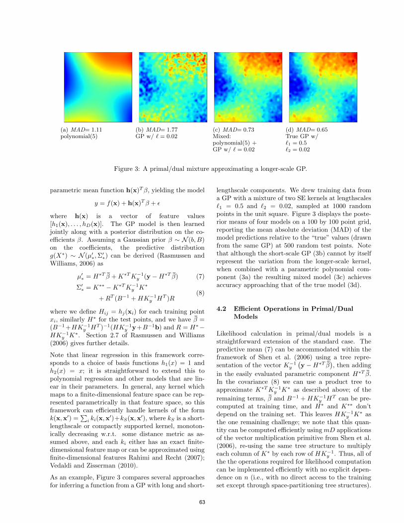
(a) MAD= 1.11polynomial(5)

(b) MAD= 1.77GP w/ ` = 0.02

(c) MAD= 0.73Mixed:polynomial(5) +GP w/ ` = 0.02

(d) MAD= 0.65True GP w/`1 = 0.5`2 = 0.02

Figure 3: A primal/dual mixture approximating a longer-scale GP.

parametric mean function h(x)Tβ, yielding the model

y = f(x) + h(x)Tβ + ε

where h(x) is a vector of feature values[h1(x), . . . , hD(x)]. The GP model is then learnedjointly along with a posterior distribution on the co-efficients β. Assuming a Gaussian prior β ∼ N (b, B)on the coefficients, the predictive distributiong(X∗) ∼ N (µ′∗,Σ

′∗) can be derived (Rasmussen and

Williams, 2006) as

µ′∗ = H∗T β +K∗TK−1y (y −H∗T β) (7)

Σ′∗ = K∗∗ −K∗TK−1y K∗

+RT (B−1 +HK−1y HT )R(8)

where we define Hij = hj(xi) for each training pointxi, similarly H∗ for the test points, and we have β =(B−1+HK−1y HT )−1(HK−1y y+B−1b) and R = H∗−HK−1y K∗. Section 2.7 of Rasmussen and Williams(2006) gives further details.

Note that linear regression in this framework corre-sponds to a choice of basis functions h1(x) = 1 andh2(x) = x; it is straightforward to extend this topolynomial regression and other models that are lin-ear in their parameters. In general, any kernel whichmaps to a finite-dimensional feature space can be rep-resented parametrically in that feature space, so thisframework can efficiently handle kernels of the formk(x,x′) =

∑i ki(x,x

′)+kS(x,x′), where kS is a short-lengthscale or compactly supported kernel, monoton-ically decreasing w.r.t. some distance metric as as-sumed above, and each ki either has an exact finite-dimensional feature map or can be approximated usingfinite-dimensional features Rahimi and Recht (2007);Vedaldi and Zisserman (2010).

As an example, Figure 3 compares several approachesfor inferring a function from a GP with long and short-

lengthscale components. We drew training data froma GP with a mixture of two SE kernels at lengthscales`1 = 0.5 and `2 = 0.02, sampled at 1000 randompoints in the unit square. Figure 3 displays the poste-rior means of four models on a 100 by 100 point grid,reporting the mean absolute deviation (MAD) of themodel predictions relative to the “true” values (drawnfrom the same GP) at 500 random test points. Notethat although the short-scale GP (3b) cannot by itselfrepresent the variation from the longer-scale kernel,when combined with a parametric polynomial com-ponent (3a) the resulting mixed model (3c) achievesaccuracy approaching that of the true model (3d).

4.2 Efficient Operations in Primal/DualModels

Likelihood calculation in primal/dual models is astraightforward extension of the standard case. Thepredictive mean (7) can be accommodated within theframework of Shen et al. (2006) using a tree repre-sentation of the vector K−1y

(y −H∗T β

), then adding

in the easily evaluated parametric component H∗T β.In the covariance (8) we can use a product tree toapproximate K∗TK−1y K∗ as described above; of the

remaining terms, β and B−1 +HK−1y HT can be pre-computed at training time, and H∗ and K∗∗ don’tdepend on the training set. This leaves HK−1y K∗ asthe one remaining challenge; we note that this quan-tity can be computed efficiently using mD applicationsof the vector multiplication primitive from Shen et al.(2006), re-using the same tree structure to multiplyeach column of K∗ by each row of HK−1y . Thus, all ofthe the operations required for likelihood computationcan be implemented efficiently with no explicit depen-dence on n (i.e., with no direct access to the trainingset except through space-partitioning tree structures).

63

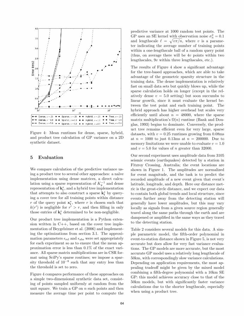
Figure 4: Mean runtimes for dense, sparse, hybrid,and product tree calculation of GP variance on a 2Dsynthetic dataset.

5 Evaluation

We compare calculation of the predictive variance us-ing a product tree to several other approaches: a naıveimplementation using dense matrices, a direct calcu-lation using a sparse representation of K−1y and denserepresentation of k∗i , and a hybrid tree implementationthat attempts to also construct a sparse k∗i by query-ing a cover tree for all training points within distancer of the query point x∗i , where r is chosen such thatk(r′) is negligible for r′ > r, and then filling in onlythose entries of k∗i determined to be non-negligible.

Our product tree implementation is a Python exten-sion written in C++, based on the cover tree imple-mentation of Beygelzimer et al. (2006) and implement-ing the optimizations from section 3.1. The approxi-mation parameters εrel and εabs were set appropriatelyfor each experiment so as to ensure that the mean ap-proximation error is less than 0.1% of the exact vari-ance. All sparse matrix multiplications are in CSR for-mat using SciPy’s sparse routines; we impose a spar-sity threshold of 10−8 such that any entry less thanthe threshold is set to zero.

Figure 4 compares performance of these approaches ona simple two-dimensional synthetic data set, consist-ing of points sampled uniformly at random from theunit square. We train a GP on n such points and thenmeasure the average time per point to compute the

predictive variance at 1000 random test points. TheGP uses an SE kernel with observation noise σ2

n = 0.1and lengthscale ` =

√vπ/n, where v is a parame-

ter indicating the average number of training pointswithin a one-lengthscale ball of a random query point(thus, on average there will be 4v points within twolengthscales, 9v within three lengthscales, etc.).

The results of Figure 4 show a significant advantagefor the tree-based approaches, which are able to takeadvantage of the geometric sparsity structure in thetraining data. The dense implementation is relativelyfast on small data sets but quickly blows up, while thesparse calculation holds on longer (except in the rel-atively dense v = 5.0 setting) but soon succumbs tolinear growth, since it must evaluate the kernel be-tween the test point and each training point. Thehybrid approach has higher overhead but scales veryefficiently until about n = 48000, where the sparsematrix multiplication’s Ω(n) runtime (Bank and Dou-glas, 1993) begins to dominate. Conversely, the prod-uct tree remains efficient even for very large, sparsedatasets, with v = 0.25 runtimes growing from 0.08msat n = 1000 to just 0.13ms at n = 200000. Due tomemory limitations we were unable to evaluate v = 1.0and v = 5.0 for values of n greater than 32000.

Our second experiment uses amplitude data from 3105seismic events (earthquakes) detected by a station inFitzroy Crossing, Australia; the event locations areshown in Figure 1. The amplitudes are normalizedfor event magnitude, and the task is to predict therecorded amplitude of a new event given that event’slatitude, longitude, and depth. Here our distance met-ric is the great-circle distance, and we expect our datato contain both global trends and local structure, sinceevents further away from the detecting station willgenerally have lower amplitudes, but this may varylocally as signals from a given source region generallytravel along the same paths through the earth and aredampened or amplified in the same ways as they travelto the detecting station.

Table 2 considers several models for this data. A sim-ple parametric model, the fifth-order polynomial inevent-to-station distance shown in Figure 5, is not veryaccurate but does allow for very fast variance evalua-tions. The GP models are more accurate, but the mostaccurate GP model uses a relatively long lengthscale of50km, with correspondingly slow variance calculations.Depending on application requirements, the most ap-pealing tradeoff might be given by the mixed modelcombining a fifth-degree polynomial with a 10km SEGP: this model achieves accuracy close to that of the50km models, but with significantly faster variancecalculations due to the shorter lengthscale, especiallywhen using a product tree.

64

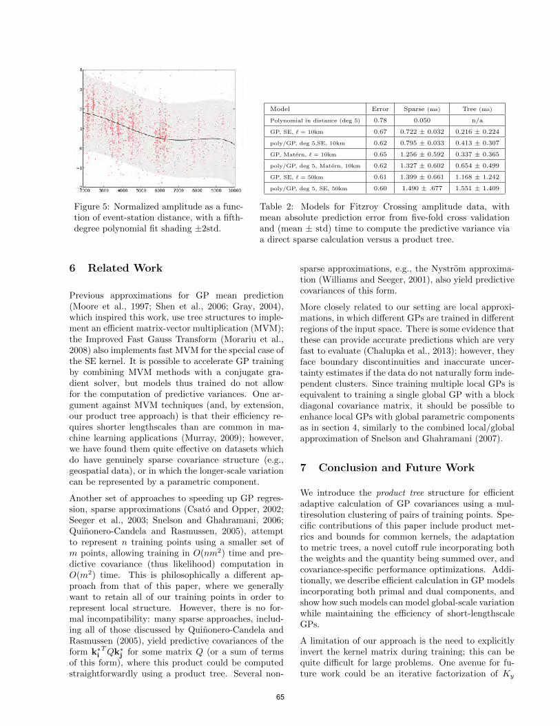
Figure 5: Normalized amplitude as a func-tion of event-station distance, with a fifth-degree polynomial fit shading ±2std.

Model Error Sparse (ms) Tree (ms)

Polynomial in distance (deg 5) 0.78 0.050 n/a

GP, SE, ` = 10km 0.67 0.722 ± 0.032 0.216 ± 0.224

poly/GP, deg 5,SE, 10km 0.62 0.795 ± 0.033 0.413 ± 0.307

GP, Matern, ` = 10km 0.65 1.256 ± 0.592 0.337 ± 0.365

poly/GP, deg 5, Matern, 10km 0.62 1.327 ± 0.602 0.654 ± 0.499

GP, SE, ` = 50km 0.61 1.399 ± 0.661 1.168 ± 1.242

poly/GP, deg 5, SE, 50km 0.60 1.490 ± .677 1.551 ± 1.409

Table 2: Models for Fitzroy Crossing amplitude data, withmean absolute prediction error from five-fold cross validationand (mean ± std) time to compute the predictive variance viaa direct sparse calculation versus a product tree.

6 Related Work

Previous approximations for GP mean prediction(Moore et al., 1997; Shen et al., 2006; Gray, 2004),which inspired this work, use tree structures to imple-ment an efficient matrix-vector multiplication (MVM);the Improved Fast Gauss Transform (Morariu et al.,2008) also implements fast MVM for the special case ofthe SE kernel. It is possible to accelerate GP trainingby combining MVM methods with a conjugate gra-dient solver, but models thus trained do not allowfor the computation of predictive variances. One ar-gument against MVM techniques (and, by extension,our product tree approach) is that their efficiency re-quires shorter lengthscales than are common in ma-chine learning applications (Murray, 2009); however,we have found them quite effective on datasets whichdo have genuinely sparse covariance structure (e.g.,geospatial data), or in which the longer-scale variationcan be represented by a parametric component.

Another set of approaches to speeding up GP regres-sion, sparse approximations (Csato and Opper, 2002;Seeger et al., 2003; Snelson and Ghahramani, 2006;Quinonero-Candela and Rasmussen, 2005), attemptto represent n training points using a smaller set ofm points, allowing training in O(nm2) time and pre-dictive covariance (thus likelihood) computation inO(m2) time. This is philosophically a different ap-proach from that of this paper, where we generallywant to retain all of our training points in order torepresent local structure. However, there is no for-mal incompatibility: many sparse approaches, includ-ing all of those discussed by Quinonero-Candela andRasmussen (2005), yield predictive covariances of theform k∗i

TQk∗j for some matrix Q (or a sum of termsof this form), where this product could be computedstraightforwardly using a product tree. Several non-

sparse approximations, e.g., the Nystrom approxima-tion (Williams and Seeger, 2001), also yield predictivecovariances of this form.

More closely related to our setting are local approxi-mations, in which different GPs are trained in differentregions of the input space. There is some evidence thatthese can provide accurate predictions which are veryfast to evaluate (Chalupka et al., 2013); however, theyface boundary discontinuities and inaccurate uncer-tainty estimates if the data do not naturally form inde-pendent clusters. Since training multiple local GPs isequivalent to training a single global GP with a blockdiagonal covariance matrix, it should be possible toenhance local GPs with global parametric componentsas in section 4, similarly to the combined local/globalapproximation of Snelson and Ghahramani (2007).

7 Conclusion and Future Work

We introduce the product tree structure for efficientadaptive calculation of GP covariances using a mul-tiresolution clustering of pairs of training points. Spe-cific contributions of this paper include product met-rics and bounds for common kernels, the adaptationto metric trees, a novel cutoff rule incorporating boththe weights and the quantity being summed over, andcovariance-specific performance optimizations. Addi-tionally, we describe efficient calculation in GP modelsincorporating both primal and dual components, andshow how such models can model global-scale variationwhile maintaining the efficiency of short-lengthscaleGPs.

A limitation of our approach is the need to explicitlyinvert the kernel matrix during training; this can bequite difficult for large problems. One avenue for fu-ture work could be an iterative factorization of Ky

65

analogous to the CG training performed by MVMmethods (Shen et al., 2006; Gray, 2004; Morariu et al.,2008). Another topic would be a better understandingof cutoff rules for the weighted sum recursion, e.g., anempirical investigation of different rules or a theoreti-cal analysis bounding the error and/or runtime of theoverall computation.

Finally, although our work has been focused primar-ily on low-dimensional applications, the use of covertrees instead of k-d trees ought to enable an exten-sion to higher dimensions. We are not aware of pre-vious work applying tree-based regression algorithmsto high-dimensional data, but as high-dimensional co-variance matrices are often sparse, this may be a nat-ural fit. For high-dimensional data that do not lieon a low-dimensional manifold, other nearest-neighbortechniques such as locality-sensitive hashing (Andoniand Indyk, 2008) may have superior properties to treestructures; the adaptation of such techniques to GPregression is an interesting open problem.

References

Andoni, A. and Indyk, P. (2008). Near-optimal hash-ing algorithms for approximate nearest neighbor inhigh dimensions. Communications of the ACM,51(1):117–122.

Bank, R. E. and Douglas, C. C. (1993). Sparse ma-trix multiplication package (SMMP). Advances inComputational Mathematics, 1(1):127–137.

Beygelzimer, A., Kakade, S., and Langford, J. (2006).Cover trees for nearest neighbor. In Proceedingsof the 23rd International Conference on MachineLearning (ICML), pages 97–104.

Chalupka, K., Williams, C. K., and Murray, I. (2013).A framework for evaluating approximation methodsfor Gaussian process regression. Journal of MachineLearning Research, 14:333–350.

Csato, L. and Opper, M. (2002). Sparse online Gaus-sian processes. Neural Computation, 14(3):641–668.

Friedman, J. H., Bentley, J. L., and Finkel, R. A.(1977). An algorithm for finding best matches inlogarithmic expected time. ACM Transactions onMathematical Software (TOMS), 3(3):209–226.

Gneiting, T. (2002). Compactly supported correla-tion functions. Journal of Multivariate Analysis,83(2):493–508.

Gray, A. (2004). Fast kernel matrix-vector multiplica-tion with application to Gaussian process learning.Technical Report CMU-CS-04-110, School of Com-puter Science, Carnegie Mellon University.

Moore, A. W., Schneider, J., and Deng, K. (1997). Ef-ficient locally weighted polynomial regression pre-

dictions. In Proceedings of the 14th InternationalConference on Machine Learning (ICML).

Morariu, V., Srinivasan, B. V., Raykar, V. C., Du-raiswami, R., and Davis, L. (2008). Automatic on-line tuning for fast Gaussian summation. Advancesin Neural Information Processing Systems (NIPS),21:1113–1120.

Murray, I. (2009). Gaussian processes and fast matrix-vector multiplies. In Numerical Mathematics in Ma-chine Learning workshop at the 26th InternationalConference on Machine Learning (ICML 2009).

Quinonero-Candela, J. and Rasmussen, C. E. (2005).A unifying view of sparse approximate Gaussianprocess regression. The Journal of Machine Learn-ing Research, 6:1939–1959.

Rahimi, A. and Recht, B. (2007). Random featuresfor large-scale kernel machines. Advances in NeuralInformation Processing Systems (NIPS), 20:1177–1184.

Rasmussen, C. and Williams, C. (2006). Gaussian Pro-cesses for Machine Learning. MIT Press.

Seeger, M., Williams, C. K., and Lawrence, N. D.(2003). Fast forward selection to speed up sparseGaussian process regression. In Artificial Intelli-gence and Statistics (AISTATS), volume 9.

Shen, Y., Ng, A., and Seeger, M. (2006). Fast Gaus-sian process regression using kd-trees. In Advancesin Neural Information Processing Systems (NIPS),volume 18, page 1225.

Snelson, E. and Ghahramani, Z. (2006). Sparse Gaus-sian processes using pseudo-inputs. In Advances inNeural Information Processing Systems (NIPS).

Snelson, E. and Ghahramani, Z. (2007). Local andglobal sparse Gaussian process approximations. InArtificial Intelligence and Statistics (AISTATS),volume 11.

Uhlmann, J. K. (1991). Satisfying general proximity/ similarity queries with metric trees. InformationProcessing Letters, 40(4):175 – 179.

Vanhatalo, J. and Vehtari, A. (2008). Modelling localand global phenomena with sparse Gaussian pro-cesses. In Proceedings of Uncertainty in ArtificialIntelligence (UAI).

Vedaldi, A. and Zisserman, A. (2010). Efficient ad-ditive kernels via explicit feature maps. In Com-puter Vision and Pattern Recognition (CVPR),2010 IEEE Conference on, pages 3539–3546. IEEE.

Williams, C. and Seeger, M. (2001). Using theNystrom method to speed up kernel machines. InAdvances in Neural Information Processing Systems(NIPS). Citeseer.

66

Latent Topic Analysis for Predicting Group Purchasing Behavior onthe Social Web

Feng-Tso Sun, Martin Griss, and Ole MengshoelElectrical and Computer Engineering Department

Carnegie Mellon University

Yi-Ting YehComputer Science Department

Stanford University

Abstract

Group-deal websites, where customers pur-chase products or services in groups, are aninteresting phenomenon on the Web. Eachpurchase is kicked off by a group initiator,and other customers can join in. Customersform communities with people with similarinterests and preferences (as in a social net-work), and this drives bulk purchasing (sim-ilar to online stores, but in larger quantitiesper order, thus customers get a better deal).In this work, we aim to better understandwhat factors influence customers’ purchasingbehavior for such social group-deal websites.We propose two probabilistic graphical mod-els, i.e., a product-centric inference model(PCIM) and a group-initiator-centric infer-ence model (GICIM), based on Latent Dirich-let Allocation (LDA). Instead of merely us-ing customers’ own purchase history to pre-dict purchasing decisions, these two modelsinclude other social factors. Using a lift curveanalysis, we show that by including social fac-tors in the inference models, PCIM achieves35% of the target customers within 5% of thetotal number of customers while GICIM isable to reach 85% of the target customers.Both PCIM and GICIM outperform randomguessing and models that do not take socialfactors into account.

1 Introduction

Group purchasing is a business model that offers var-ious deals-of-the-day and an extra discount depend-ing on the size of the purchasing group. After group-deal websites, such as Groupon and LivingSocial, havegained attention, similar websites, such as ihergo1

1http://www.ihergo.com

and Taobao,2 have introduced social networks as afeature for their users. These group-deal websites pro-vide an interesting hybrid of social networks (e.g.,Facebook.com and LinkedIn.com) and online stores(e.g., Amazon.com and Buy.com). Customers formcommunities with people with similar interests andpreferences (as in a social network), and this drivesbulk purchasing (similar to online stores, but in largerquantities per order, thus customers get a better deal).As we see more and more social interactions amongcustomers in group-deal websites, it is critical to un-derstand the interplay between social factors and pur-chasing preferences.

In this paper, we analyze a transactional datasetfrom the largest social group-deal website in Taiwan,ihergo.com. Figure 1 shows a screenshot from thegroup-deal page of ihergo.com. Each group-purchasingevent on ihergo.com consists of three major compo-nents: (1) a group initiator, (2) a number of groupmembers, and (3) a group-deal product. A group ini-tiator starts a group-purchasing event for a specificgroup-deal product. While this event will be postedpublicly, the group initiator’s friends will also be no-tified. A user can choose to join the purchasing eventto become a group member.

Group initiators play important roles on this kind ofgroup-deal websites. Usually, the merchants would of-fer incentives for the group initiators to initiate group-purchasing events by giving them products for free ifthe size of the group exceeds some threshold. In addi-tion, to save shipping costs, the group can choose tohave the whole group-deal order shipped to the initia-tor. In this case, the initiator would need to distributethe products to group members in person. Hence, thegroup members usually reside or work in the proximityof the group initiator. Sometimes, they are friends orco-workers of the initiator.

Understanding customers’ purchasing behavior in this

2http://www.taobao.com

67

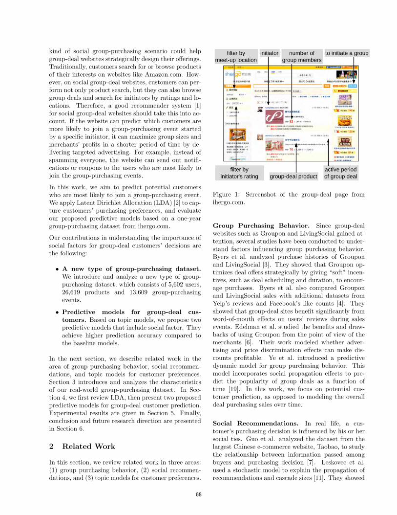
kind of social group-purchasing scenario could helpgroup-deal websites strategically design their offerings.Traditionally, customers search for or browse productsof their interests on websites like Amazon.com. How-ever, on social group-deal websites, customers can per-form not only product search, but they can also browsegroup deals and search for initiators by ratings and lo-cations. Therefore, a good recommender system [1]for social group-deal websites should take this into ac-count. If the website can predict which customers aremore likely to join a group-purchasing event startedby a specific initiator, it can maximize group sizes andmerchants’ profits in a shorter period of time by de-livering targeted advertising. For example, instead ofspamming everyone, the website can send out notifi-cations or coupons to the users who are most likely tojoin the group-purchasing events.

In this work, we aim to predict potential customerswho are most likely to join a group-purchasing event.We apply Latent Dirichlet Allocation (LDA) [2] to cap-ture customers’ purchasing preferences, and evaluateour proposed predictive models based on a one-yeargroup-purchasing dataset from ihergo.com.

Our contributions in understanding the importance ofsocial factors for group-deal customers’ decisions arethe following:

• A new type of group-purchasing dataset.We introduce and analyze a new type of group-purchasing dataset, which consists of 5,602 users,26,619 products and 13,609 group-purchasingevents.

• Predictive models for group-deal cus-tomers. Based on topic models, we propose twopredictive models that include social factor. Theyachieve higher prediction accuracy compared tothe baseline models.

In the next section, we describe related work in thearea of group purchasing behavior, social recommen-dations, and topic models for customer preferences.Section 3 introduces and analyzes the characteristicsof our real-world group-purchasing dataset. In Sec-tion 4, we first review LDA, then present two proposedpredictive models for group-deal customer prediction.Experimental results are given in Section 5. Finally,conclusion and future research direction are presentedin Section 6.

2 Related Work

In this section, we review related work in three areas:(1) group purchasing behavior, (2) social recommen-dations, and (3) topic models for customer preferences.

to initiate a groupnumber of group members

initiator

group-deal productfilter by

initiator's ratingactive period of group deal

filter by meet-up location

Figure 1: Screenshot of the group-deal page fromihergo.com.

Group Purchasing Behavior. Since group-dealwebsites such as Groupon and LivingSocial gained at-tention, several studies have been conducted to under-stand factors influencing group purchasing behavior.Byers et al. analyzed purchase histories of Grouponand LivingSocial [3]. They showed that Groupon op-timizes deal offers strategically by giving “soft” incen-tives, such as deal scheduling and duration, to encour-age purchases. Byers et al. also compared Grouponand LivingSocial sales with additional datasets fromYelp’s reviews and Facebook’s like counts [4]. Theyshowed that group-deal sites benefit significantly fromword-of-mouth effects on users’ reviews during salesevents. Edelman et al. studied the benefits and draw-backs of using Groupon from the point of view of themerchants [6]. Their work modeled whether adver-tising and price discrimination effects can make dis-counts profitable. Ye et al. introduced a predictivedynamic model for group purchasing behavior. Thismodel incorporates social propagation effects to pre-dict the popularity of group deals as a function oftime [19]. In this work, we focus on potential cus-tomer prediction, as opposed to modeling the overalldeal purchasing sales over time.

Social Recommendations. In real life, a cus-tomer’s purchasing decision is influenced by his or hersocial ties. Guo et al. analyzed the dataset from thelargest Chinese e-commerce website, Taobao, to studythe relationship between information passed amongbuyers and purchasing decision [7]. Leskovec et al.used a stochastic model to explain the propagation ofrecommendations and cascade sizes [11]. They showed

68

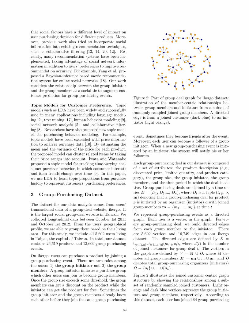
that social factors have a different level of impact onuser purchasing decision for different products. More-over, previous work also tried to incorporate socialinformation into existing recommendation techniques,such as collaborative filtering [13, 14, 20, 12]. Re-cently, many recommendation systems have been im-plemented, taking advantage of social network infor-mation in addition to users’ preferences to improve rec-ommendation accuracy. For example, Yang et al. pro-posed a Bayesian-inference based movie recommenda-tion system for online social networks [18]. Our workconsiders the relationship between the group initiatorand the group members as a social tie to augment cus-tomer prediction for group-purchasing events.

Topic Models for Customer Preference. Topicmodels such as LDA have been widely and successfullyused in many applications including language model-ing [2], text mining [17], human behavior modeling [9],social network analysis [5], and collaborative filter-ing [8]. Researchers have also proposed new topic mod-els for purchasing behavior modeling. For example,topic models have been extended with price informa-tion to analyze purchase data [10]. By estimating themean and the variance of the price for each product,the proposed model can cluster related items by takingtheir price ranges into account. Iwata and Watanabeproposed a topic model for tracking time-varying con-sumer purchase behavior, in which consumer interestsand item trends change over time [9]. In this paper,we use LDA to learn topic proportions from purchasehistory to represent customers’ purchasing preferences.

3 Group-Purchasing Dataset

The dataset for our data analysis comes from users’transactional data of a group-deal website, ihergo. Itis the largest social group-deal website in Taiwan. Wecollected longitudinal data between October 1st 2011and October 1st 2012. From the users’ geographicalprofile, we are able to group them based on their livingarea. For this study, we include all 5,602 users livingin Taipei, the capital of Taiwan. In total, our datasetcontains 26,619 products and 13,609 group-purchasingevents.

On ihergo, users can purchase a product by joining agroup-purchasing event. There are two roles amongthe users: 1) the group initiator and 2) the groupmember. A group initiator initiates a purchase groupwhich other users can join to become group members.Once the group size exceeds some threshold, the groupmembers can get a discount on the product while theinitiator can get the product for free. Sometimes thegroup initiator and the group members already knoweach other before they join the same group-purchasing

Figure 2: Part of group deal graph for ihergo dataset:illustration of the member-centric relationships be-tween group members and initiators from a subset ofrandomly sampled joined group members. A directededge is from a joined customer (dark blue) to an ini-tiator (light orange).

event. Sometimes they become friends after the event.Moreover, each user can become a follower of a groupinitiator. When a new group-purchasing event is initi-ated by an initiator, the system will notify his or herfollowers.

Each group-purchasing deal in our dataset is composedof a set of attributes: the product description (e.g.,discounted price, limited quantity, and product cate-gory), the group size, the group initiator, the groupmembers, and the time period in which the deal is ac-tive. Group-purchasing deals are defined by a time se-ries D = (D1, D2,..., Dn), where Di is a tuple (t, p, o,m) denoting that a group-purchasing deal for productp is initiated by an organizer (initiator) o with joinedgroup members m = m1, ..., mk at time t.

We represent group-purchasing events as a directedgraph. Each user is a vertex in the graph. For ev-ery group-purchasing deal, we build directed edgesfrom each group member to the initiator. Thereare 5,602 vertices and 16,749 edges in our ihergodataset. The directed edges are defined by E =∪i∈[1,n] ∪j∈[1,d(i)](mi,j , oi), where d(i) is the numberof joined customers for group deal i. The vertices inthe graph are defined by V = M ∪ O, where M de-notes all group members M = m1 ∪ . . .∪mn and Odenotes total group-purchasing organizers (initiators)O = o1∪ . . .∪on.

Figure 2 illustrates the joined customer centric graphstructure by showing the relationships among a sub-set of randomly sampled joined customers. Light or-ange and dark blue vertices represent the group initia-tors and group members, respectively. According tothis dataset, each user has joined 84 group-purchasing

69

node out degree10 20 30

0

0.3de

gree

dist

ribut

ion

0.2

0.1

0 5 10 15 20 25 30 35

0.00

0.10

0.20

0.30

node degree

degr

ee.d

istri

butio

n(g,

mod

e =

c("o

ut"))

0

Figure 3: Node out-degree distribution for the group-purchasing graph of ihergo. 80% of the users followfive or fewer initiators.

events on average. However, one interesting obser-vation from the graph is that the number of outgo-ing edges from dark blue vertices is far less than 84.This property can be even clearly seen from the out-degree distribution for the overall group-purchasinggraph shown in Figure 3. We see that 80% of theusers only join group-purchasing events initiated by5 or fewer different initiators. Group members havea tendency to repeatedly join group-purchasing initi-ated by a relatively small number of initiators theyco-bought with before.

Therefore, we hypothesize that customers’ purchasingdecisions are not only influenced by their own purchas-ing preferences but also strongly influenced by who thegroup initiator is. In the next section, we propose twonew models to predict which customers are most likelyto join a particular group-purchasing event.

4 Methodology

In this section, we first describe in Section 4.1 how weapply topic modeling to learn user purchasing pref-erences under the group-purchasing scenario. Duringthe training phase, we compute for each user a mix-ture topic proportion by combining topic proportionsof this user and the initiators with whom this user hasco-bought products.

Given a new group-purchasing event, we would like topredict which customers are more likely to join. Wepropose two predictive models in Section 4.2. Onemodel, which we denote as the product-centric infer-ence model (PCIM), computes the posterior probabil-ity that a user would purchase this product given his orher mixture topic proportion. The other model, whichwe denote the group initiator centric inference model(GICIM), computes the posterior probability that auser would join the group-purchasing event initiatedby this initiator given user’s or initiator’s mixture topicproportion.

↵

z

x

K UNu

Figure 4: Graphical model representation of the latentDirichlet allocation model.

4.1 Topic Model for User PurchasingPreference

We use topic modeling to characterize a user’s pur-chasing preference. In particular, we apply LDA to ourgroup-purchasing dataset. In a typical LDA model fortext mining [2], a document is a mixture of a numberof hidden topics which can be represented by a multi-nomial distribution, i.e. the topic proportion. A wordcan belong to one or more hidden topics with differentprobabilities. Figure 4 shows the graphical model forLDA. LDA is a generative model where each word ina document is generated by two steps: 1) sample atopic from its topic distribution and 2) draw a wordfrom that topic. One can also use Bayesian inferenceto learn the particular topic proportion of each docu-ment.

In our model, we treat a user’s purchase history as adocument. Each purchased product can be seen as aword in a document. We make an analogy betweentext documents and purchasing patterns as shown inTable 1. We replace words with each purchased prod-uct and a document is one user’s purchasing history.Assume that there are U users in our training data.Let U denote the set of users. Each user u ∈ U hasa vector of purchased products xu = xunNu

n=1 whereNu is the number of products that user u purchased.

The generative process of the LDA model for learninga user’s purchasing preferences is described as follow-ing. Each user u has his or her own topic proportion(i.e., purchasing preference) θu that is sampled froma Dirichlet distribution. Next, for each product xun

purchased by user u, a topic zun is firstly chosen fromthe user’s topic proportion θu. Then, a product xun

is drawn from the multinomial distribution φzun. To

estimate θu and φzun, we use the collapsed Gibbs sam-

pling method [15].

70

Symbol Description for Group Purchase History Description for Text DocumentsU Number of users Number of documentsK Number of latent topics Number of latent topicsNu Number of purchased products of user u Number of words of document uzun Latent co-purchasing category of nth product Latent topic of nth word of document uxun nth purchased product of user u nth word of document uθu Latent co-purchasing category proportion for user u Topic proportin for document uφk Multinomial distribution over products for topic k Mult. distribution over words for topic kα Dirichlet prior parameters for all θu Dirichlet prior parameters for all θu

β Dirichlet prior parameters for all φk Dirichlet prior parameters for all φk

Table 1: Latent Dirichlet allocation plate model notation

4.2 Proposed Models for PredictingGroup-Deal Customers

A group-purchasing event contains two kinds of criticalinformation: who the group initiator is and what thegroup-deal product is. Our goal is to predict whichcustomers are more likely to join a specific group-purchasing event. Intuitively, one may think thatwhether a customer would join a group-purchasingevent solely depends on what the group-deal productis. However, from our observations in the dataset, wehypothesize a correlation between a customer’s pur-chasing decision and who the group initiator is. There-fore, we would like to study how these two kinds ofgroup-purchasing information affect the prediction ac-curacy by asking two questions:

1. What is the likelihood that a customer would jointhe event given what the group-deal product is?

2. What is the likelihood that a customer would jointhe event given who the group-initiator is?

This leads to our two proposed predictive models,the product centric inference model (PCIM ) and thegroup initiator centric inference model (GICIM ).

4.2.1 Product Centric Inference Model(PCIM)

Figure 5(a) shows the graphical structure of PCIM.For each user, we train a PCIM. PCIM computes theposterior probability that a user would purchase aproduct given his or her mixture topic proportion. LetC denote the user’s own topic proportion, which welearned from LDA. Suppose that this user has joinedgroup-purchasing events initiated by n group initia-tors, we use Iin

i=1 to denote the learned topic pro-portions of these initiators. Our model computes theweighted topic proportions of initiators W by linearlycombining Iin

i=1 with the frequency distribution thatthe user co-bought products with them.

Intuitively, if a user joins a group-purchasing eventinitiated by a group initiator, they might share sim-ilar interests. Therefore, our model characterizes theuser’s purchasing preferences by a weighting schemethat combines C and W with a weighting parameterw. We use M to denote such a mixture topic propor-tion which encodes the overall purchasing preferencesof the user.

Let P denote the product random variable. Ω(P) =p1, ..., pm, where pi is the product. From each datarecord Di ∈D , we have a tuple (ti, pi, oi, mi) andknow what group-deal product pi corresponds to a par-ticular group-purchasing event ei. Our goal is to com-pute Pr(P = pi), the probability that the user wouldjoin a group-purchasing event ei to buy a product pi.

Given the topic proportion C and Iini=1 correspond-

ing to the user and the weighting parameter w, we areable to compute

Pr(P ) =∑

Y=Xp\P

Pr(P,Y) (1)

where Xp = P,M,C,W, I1, ..., In; P a is productrandom variable; M is a mixture topic proportion.

To predict which users are more likely to join a group-purchasing event, we rank P(u1)

pi , . . . ,P(uU )pi in de-

scending order where u1, . . . , uU denotes the set ofusers in our dataset and P(uj)

pi denotes Pr(P = pi) ofuser uj .

4.2.2 Group Initiator Centric InferenceModel (GICIM)

The graphical illustration of GICIM is shown in Figure5(b). GICIM computes the posterior probability thata user would join a group-purchasing event initiatedby a particular initiator given user’s or initiator’s mix-ture topic proportion. GICIM and PCIM only differin their leaf nodes. While PCIM considers only whatthe group-deal product is, GICIM models our observa-tion that the decision of whether or not a user joins a

71

Figure 5: Our proposed models for predicting poten-tial customers given a group-purchasing event. (a)Product centric inference model (PCIM). (b) Groupinitiator centric inference model (GICIM).

group-purchasing event is strongly influenced by whothe group initiator of that event is.

Let I denote the initiator random variable and ii de-note the initiator of the group-purchasing event ei.Again, from each data record Di ∈D , we know who thegroup initiator is. Instead of evaluating Pr(P = pi) asin PCIM, we use GICIM to compute

Pr(I) =∑

Y=Xp\I

Pr(I,Y) (2)

where Xp = I, M, C, W, I1, ..., In; I is an initiatorrandom variable; M is a mixture topic proportion.

To predict which users are more likely to join a group-purchasing event ei, we rank P(u1)

oi , . . . ,P(uU )oi in de-

scending order where u1, . . . , uU denotes the set ofusers in our dataset and P(uj)

oi denotes Pr(I = oi) ofuser uj .

5 Experimental Evaluation

5.1 Data Pre-processing

We evaluate the proposed PCIM and GICIM mod-els with the ihergo group-purchasing dataset. In or-der to capture meaningful user purchasing preferences,we remove users who purchased fewer than 10 prod-ucts during the pre-processing step. We use ten-foldcross-validation to generate our training and testingdatasets.

5.2 LDA Topic Modeling on GroupPurchasing Dataset

To measure the performance of LDA for different num-ber of topics (20, 40, 60, 80, 100) in our group-

4000

6000

8000

100 200 300 400 500#iterations

perp

lexi

ty

model_type

20

40

60

80

100

Number of Iterations

Perp

lexi

ty

100 2000 400

6000

4000

8000

300

Number of Topics

500

4000

6000

8000

100 200 300 400 500#iterations

perp

lexi

ty

model_type

20

40

60

80

100

20406080100

Figure 6: Perplexity as function of collapsed Gibbssampling iterations for different number of topics usedin LDA.

purchasing dataset, we compute the perplexity. Itmeasures how well the model generalizes and predictsnew documents [2]. Figure 6 shows that the per-plexity decreases as the number of iteration increasesand converges within 200 iterations. In addition, aswe increase the number of topics, the perplexity de-creases. Unless mentioned specifically, all topic pro-portions used in our experiments are learned with LDAusing 100 topics.

Figure 7 shows three example product topics learnedby LDA using 100 topics. Each table shows the tenproducts that are most likely to be bought in thattopic. Columns in the table represent the productname, the probability of the product being purchasedin that topic, and the ground-truth category of theproduct, respectively. We see that Topic 1 is about“pasta.” It contains a variety of cooked pasta andpasta sauce. Topic 18 and 53 are respectively about“bread and cakes” and “women accessories.”

Figure 8 shows the topic proportions of four randomlyselected users learned by LDA using 60 topics. We seethat different users have distinguishable topic propor-tions, representing their purchasing preferences. Forexample, user #3617 purchased many products thatare about “beauty” and “clothing” so her or his topicproportion has higher probabilities at topic 4 and topic17. Similarly, user #39 tends to buy products in the“dim sum” category which can be represented in heror his topic proportion.

72

(a) User #3617 (b) User #5 (c) User #2618 (d) User #39

prob

abili

ty

topic0 20 40 60

0

0.1

0.2

0.00

0.05

0.10

0.15

0.20

0 20 40 60topic

prob

types_tp

buyer_tp

clothingbeauty

topic0 20 40 60

0

0.1

0.2

0.00

0.05

0.10

0.15

0.20

0 20 40 60topic

prob

types_tp

buyer_tp

microwavable food

topic0 20 40 60

0

0.1

0.2

0.00

0.05

0.10

0.15

0.20

0 20 40 60topic

prob

types_tp

buyer_tp

dim sum

topic0 20 40 60

0

0.1

0.2

0.00

0.05

0.10

0.15

0.20

0 20 40 60topic

prob

types_tp

buyer_tp

juicecookies

Figure 8: Examples illustrating learned topic proportions of four randomly selected users. For user #3617, thetwo most probable topics are “beauty” and “clothing”.

(a) Topic 1, "pasta"

(b) Topic 18, "bread and cakes"

(c) Topic 53, "women accessories"

Symbol DescriptionU Number of usersI Number of productsK Number of latent topicsNu Number of purchased products of user u

zun Latent topic of nth purchased product of user u

xun nth purchased product of user u

u Topic proportion for user u, u=ukKk=1, uk 0,

KPk=1

uk = 1

k Multinomial distribution over products for topic k, k=kiIi=1, ki 0,

IPi=1

ki = 1

↵ Dirichlet prior parameters for all u

Dirichlet prior parameters for all k

Table 1: LDA plate model notation

their purchase preference. For example, user2 purchasedmany products that are most likely in ”Seafood” category,hence, his topic proportion has higher probability at topic 4,”Seafood” category. Similarly, user10 tends to buy productsin ”Pasta” category which can be represented in his topicproportion.

5.3 Performance of PCIM and GICIMTo evaluate the performance of PCIM and GICIM, we use

lift chart to measure the e↵ectiveness of prediction result forgroup-buying buyers. In a lift chart, the x-axis represents isthe percentage of users sorted by our prediction score andthe y-axis is the cumulative percentage of the ground-truthbuyers we would predict.

For the evaluation of PCIM and GICIM, we use users’topic proportions and product’s topic proportion as input.Figure 7 shows the performance of PCIM model with dif-ferent weighting of co-occurrence initiator influence. As wecan observe, PCIM with user’s topic proportion only (w=1)has better prediction with 25% of predicted buyers. How-ever, the performance degrades and is worse than randomsample (baseline) after including 65% of predicted users.This e↵ect can be explained that users who have no strongpurchase preference have low prediction score and PCIMmodel cannot correctly predict. On the other hand, us-ing co-occurrence initiator topic proportions (w<1), PCIMachieves better prediction after including 40% of predictedusers. Overall performance is better than random samplewith co-occurrence initiator topic proportions only (w=0),though the positive response rate is slightly lower than user’stopic proportion only setting (w=1) before including 40%predicted users.

Figure 8 demonstrates the performance of GICIM modelwith di↵erent weighting of co-occurrence initiator influence.GICIM model significantly outperforms PCIM and it achieves90% positive response by only including 10% predicted buy-ers. The performance change due to the di↵erent weightingof co-occurrence initiator influence is not as significant asin PCIM. The high prediction rate of GICIM explains thatmost of users choose join the purchase group or not basedon who the group initiator is.

In Figure 10, we found PCIM and GICIM models havethe consistent performance over di↵erent product categories(e.g., food, bodycare, apparel, toys, and living). Moreover,GICIM outperforms PICIM over all product categories.

product prob. categoryChicken pasta (cream sauce) 0.0197 PastaChicken pasta (pesto sauce) 0.0193 PastaPork pasta (tomato sauce) 0.0167 PastaPork steak 0.0155 MeatBacon pasta (cream sauce) 0.0153 PastaSpicy pasta (tomato sauce) 0.0149 PastaClam garlic linguine 0.0146 PastaTomato sauce pasta 0.0142 PastaGerman sausage sauce 0.0132 PastaItalian pasta (cooked) 0.0129 Pasta

Table 2: Illustration of product topics created byLDA. Category is from ground truth.

product prob. categoryHam sandwich 0.0101 BreadCheese sandwich 0.0089 BreadMilk bar cookie 0.0080 CookieCherry chocolate tart 0.0078 CakeCheese roll 0.0077 CakeCheese almond tart 0.0074 CakeTaro toast 0.0073 BreadCreme Brulee 0.0073 CakeRaisin toast 0.0071 BreadWheat ham sandwich 0.0070 Bread

Table 3: Topic 18.

product prob. categoryKnit Hat 0.0169 AccessoryKnit Scarf 0.0165 AccessoryLegging 0.0133 ClothingWool scarf 0.0120 AccessoryLong Pant 0.0111 ClothingCotton Socks 0.0099 AccessoryWool Gloves 0.0097 AccessoryFacial Masks 0.0090 BodyCareWool socks 0.0088 AccessoryBrown knit scarf 0.0081 Accessory

Table 4: Topic 53.





KPk=1

uk = 1


IPi=1

ki = 1













Table 3: Topic 18.


Table 4: Topic 53.





KPk=1

uk = 1


IPi=1

ki = 1













Table 3: Topic 18.


Table 4: Topic 53.

Product

Product

Product

Prob. Category

Prob. Category

Prob. Category

PastaPastaPasta

PastaPastaPastaPastaPastaPastaMeat

BreadBreadCookie

BreadBreadCakeBreadCakeCakeCake

AccessoryAccessoryClothing

AccessoryAccessoryBody CareAccessoryAccessoryClothingAccessory

Figure 7: Illustration of product topics learned byLDA using 100 topics. Category is from ground truth.

5.3 Performance of PCIM and GICIM

We use lift charts to measure the effectiveness ofPCIM and GICIM for predicting group-purchasingcustomers. In a lift chart, the x-axis represents thepercentage of users sorted by our prediction score andthe y-axis represents the cumulative percentage of theground-truth customers we would predict. For all liftcharts shown in this section, we also include two base-line models for comparison. One baseline model isto predict potential customers by randomly samplingfrom the set of users. Therefore, it is a straight linewith slope 1.0 on the lift chart. Another baselinemodel, which we call category frequency, is to predictcustomers with the most frequent purchase history ina given product category. Specifically, to predict po-tential customers given a group-deal product category,we rank each customer in descending order of theirnormalized purchase frequency for the given productcategory.

Effect of w. We first measure the effect of the weight-ing parameter w in PCIM, which is shown in Figure 9.The particular w controls how much the user’s owntopic proportion is used in the mixture topic propor-tion. For example, w = 1 means that only the user’sown topic proportion is used as the mixture topic pro-portion. We see that for all w values, PCIM performsmuch better than the baseline models between 0% and25% of the customers predicted. For instance, PCIMis able to reach 50% of the targeted customers whilethe two baseline models only reach respectively 25%and 40% of the customers.

We also see that with w = 1, the curve first rises veryfast, then flattens between 25% and 50%. It evenperforms worse than the baseline models starting ataround 60% of the customers predicted; however thisis the least interesting part of the curve. The intuitionbehind this behavior is that with w = 1, PCIM is goodat predicting customers who have strong purchasingpreferences that match the targeted group-deal prod-uct. On the other hand, for users without such strongpurchasing preferences, the model is not able to per-

73

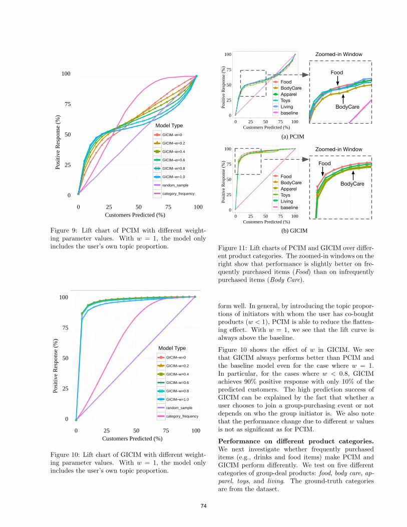
Customers Predicted (%)

Posit

ive

Resp

onse

(%)

25 50

0

0 100

50

25

75

75

100

0

25

50

75

100

0 25 50 75 100Buyers Predicted (%)

Posit

ive R

espo

nses

(%)

model_type

PCIM−w=0

PCIM−w=0.2

PCIM−w=0.4

PCIM−w=0.6

PCIM−w=0.8

PCIM−w=1.0

random_sample

category_frequency

0

25

50

75

100


Posi

tive

Res

pons

es(%

)

model_type

GICIM−w=0

GICIM−w=0.2

GICIM−w=0.4

GICIM−w=0.6

GICIM−w=0.8

GICIM−w=1.0

random_sample

category_frequency

Model Type

Figure 9: Lift chart of PCIM with different weight-ing parameter values. With w = 1, the model onlyincludes the user’s own topic proportion.


Posit

ive

Resp

onse

(%)

25 50

0

0 100

50

25

75

75

100

0

25

50

75

100


Posi

tive

Res

pons

es(%

)

model_type

GICIM−w=0

GICIM−w=0.2

GICIM−w=0.4

GICIM−w=0.6

GICIM−w=0.8

GICIM−w=1.0

random_sample

category_frequency

Model Type

Figure 10: Lift chart of GICIM with different weight-ing parameter values. With w = 1, the model onlyincludes the user’s own topic proportion.

0

25

50

75

100


Posi

tive

Res

pons

es(%

)

model_type

PCIM−Food

PCIM−BodyCare

PCIM−Apparel

PCIM−Toys,Kids&Baby

PCIM−Living

random_sample

(a) PCIM

(b) GICIM


Posit

ive

Resp

onse

(%)

25 50 0

0 100

50

25

75

75

100

0

25

50

75

100


Posi

tive

Res

pons

es(%

)

model_type

GICIM−Food

GICIM−BodyCare

GICIM−Apparel

GICIM−Toys,Kids&Baby

GICIM−Living

PCIM−Food

PCIM−BodyCare

PCIM−Apparel


PCIM−Living

random_sample

0

25

50

75

100


Posi

tive

Res

pons

es(%

)model_type

GICIM−Food

GICIM−BodyCare

GICIM−Apparel


GICIM−Living

PCIM−Food

PCIM−BodyCare

PCIM−Apparel


PCIM−Living

random_sample

FoodBodyCareApparel

LivingToys

baseline

0

25

50

75

100


Posi

tive

Res

pons

es(%

)

model_type

PCIM−Food

PCIM−BodyCare

PCIM−Apparel


PCIM−Living

random_sample

FoodBodyCareApparel

LivingToys

baseline

0

25

50

75

100


Posi

tive

Res

pons

es(%

)

model_type

GICIM−Food

GICIM−BodyCare

GICIM−Apparel


GICIM−Living

PCIM−Food

PCIM−BodyCare

PCIM−Apparel


PCIM−Living

random_sample

Food

BodyCare0

25

50

75

100


Posi

tive

Res

pons

es(%

)

model_type

PCIM−Food

PCIM−BodyCare

PCIM−Apparel


PCIM−Living

random_sample

Food

BodyCare

Zoomed-in Window

Zoomed-in Window

Customers Predicted (%)Po

sitiv

e Re

spon

se (%

)25 50

00 100

50

25

75

75

100

Figure 11: Lift charts of PCIM and GICIM over differ-ent product categories. The zoomed-in windows on theright show that performance is slightly better on fre-quently purchased items (Food) than on infrequentlypurchased items (Body Care).

form well. In general, by introducing the topic propor-tions of initiators with whom the user has co-boughtproducts (w < 1), PCIM is able to reduce the flatten-ing effect. With w = 1, we see that the lift curve isalways above the baseline.

Figure 10 shows the effect of w in GICIM. We seethat GICIM always performs better than PCIM andthe baseline model even for the case where w = 1.In particular, for the cases where w < 0.8, GICIMachieves 90% positive response with only 10% of thepredicted customers. The high prediction success ofGICIM can be explained by the fact that whether auser chooses to join a group-purchasing event or notdepends on who the group initiator is. We also notethat the performance change due to different w valuesis not as significant as for PCIM.

Performance on different product categories.We next investigate whether frequently purchaseditems (e.g., drinks and food items) make PCIM andGICIM perform differently. We test on five differentcategories of group-deal products: food, body care, ap-parel, toys, and living. The ground-truth categoriesare from the dataset.

74

0

25

50

75

100


Posi

tive

Res

pons

es(%

)

model_type

GICIM−w=0−k=20

GICIM−w=0−k=40

GICIM−w=0−k=60

GICIM−w=0−k=80

GICIM−w=0−k=100

random_sample

0

25

50

75

100


Posi

tive

Res

pons

es(%

)

model_type

GICIM−w=1−k=20

GICIM−w=1−k=40

GICIM−w=1−k=60

GICIM−w=1−k=80

GICIM−w=1−k=100

random_sample

0

25

50

75

100


Posi

tive

Res

pons

es(%

)

model_type

PCIM−w=0−k=20

PCIM−w=0−k=40

PCIM−w=0−k=60

PCIM−w=0−k=80

PCIM−w=0−k=100

random_sample

0

25

50

75

100


Posi

tive

Res

pons

es(%

)

model_type

PCIM−w=1−k=20

PCIM−w=1−k=40

PCIM−w=1−k=60

PCIM−w=1−k=80

PCIM−w=1−k=100

random_sample

(a) PCIM, w = 0 (b) PCIM, w = 1

(c) GICIM, w = 0 (d) GICIM, w = 1

k=20

0

25

50

75

100


Posi

tive

Res

pons

es(%

)

model_type

GICIM−w=1−k=20

GICIM−w=1−k=40

GICIM−w=1−k=60

GICIM−w=1−k=80

GICIM−w=1−k=100

random_sample

k=40k=60k=80k=100baseline

k=20

0

25

50

75

100


Posi

tive

Res

pons

es(%

)

model_type

GICIM−w=1−k=20

GICIM−w=1−k=40

GICIM−w=1−k=60

GICIM−w=1−k=80

GICIM−w=1−k=100

random_sample


k=20

0

25

50

75

100


Posi

tive

Res

pons

es(%

)

model_type

GICIM−w=1−k=20

GICIM−w=1−k=40

GICIM−w=1−k=60

GICIM−w=1−k=80

GICIM−w=1−k=100

random_sample


k=20

0

25

50

75

100


Posi

tive

Res

pons

es(%

)

model_type

GICIM−w=1−k=20

GICIM−w=1−k=40

GICIM−w=1−k=60

GICIM−w=1−k=80

GICIM−w=1−k=100

random_sample



Posit

ive

Resp

onse

(%)

25 50 0

0 100

50

25

75

75

100


Posit

ive

Resp

onse

(%)

25 50 0

0 100

50

25

75

75

100


Posit

ive

Resp

onse

(%)

25 50 0

0 100

50

25

75

75

100

Customers Predicted (%)Po

sitiv

e Re

spon

se (%

)

25 50 0

0 100

50

25

75

75

100

Figure 12: Lift charts of PCIM and GICIM over dif-ferent number of topics.

Figure 11 shows the results. We see that, for all prod-uct categories tested, GICIM still performs better thanPCIM. Moreover, from Figure 11, we see that bothmodels are slightly better at predicting potential cus-tomers for the food category than for the body carecategory. We hypothesize that this may be related tothe fact that purchases in the food category are morefrequent and predictable compared to purchases in thebody care category. A customers may buy one or moreproducts in the food category repeatedly, while thesame does not appear to be the case for all products inthe body care category. For example, once someone haspurchased a sunscreen spray (a product in body care),they are probably unlikely to buy it again, at least forthe time span that our dataset covers. However, notethat the differences between categories in Figure 11 aresmall, and developing a better understanding of themis an area of future research.

Effect of different number of topics. We ranPCIM and GICIM on different number of topics usedin LDA. Results are given in Figure 12. We find thatincreasing the number of topics increases predictionaccuracy for both models. This agrees with the aboveperplexity analysis that higher number of topics resultsin better performance.

6 Conclusion

In this paper, we study group-purchasing patternswith social information. We analyze a real-worldgroup-purchasing dataset (5,602 users, 26,619 prod-ucts, and 13,609 events) from ihergo.com. To thebest of our knowledge, we are the first to ana-lyze the group-purchasing scenario where each group-purchasing event is started by an initiator. Under thiskind of social group-purchasing framework, each userbuilds up social ties with a set of group initiators. Ouranalysis of the dataset shows that a user usually joinsgroup-purchasing events initiated by a certain and rel-atively small number of initiators. That is, if a user hasco-bought a group-deal product with a group initia-tor, he or she is more likely to join a group-purchasingevent started by that initiator again.

We develop two models to predict which users are mostlikely to join a group-purchasing event. Experimentalresults show that by including the weighted topic pro-portions of the initiators, we achieve higher predictionaccuracy. We also find that whether a user decides tojoin a group-purchasing event is strongly influenced bywho the group initiator of that event is.

Our model can be further improved in several ways.First, we can use Labeled LDA [16] by exploiting theground-truth category of the products or user profilefrom the dataset. Second, we can incorporate otherinformation such as the geographical and demographicinformation of users, and the seasonality of products ina more complex topic model. We are also interested ininvestigating the model to deal with cold start, where anew user or group-deal product is added to the system.

Acknowledgments

We want to thank Kuo-Chun Chang from ihergo.comfor his cooperation and the use of ihergo dataset. Thismaterial is based, in part, upon work supported byNSF award CCF0937044 to Ole Mengshoel.

References

[1] G. Adomavicius and A. Tuzhilin. Toward the nextgeneration of recommender systems: A survey ofthe state-of-the-art and possible extensions. IEEETrans. on Knowl. and Data Eng., 17(6), June2005.

[2] D. M. Blei, A. Y. Ng, and M. I. Jordan. LatentDirichlet allocation. J. Mach. Learn. Res., 3, Mar.2003.

[3] J. W. Byers, M. Mitzenmacher, M. Potamias, andG. Zervas. A month in the life of Groupon. CoRR,2011.

75

[4] J. W. Byers, M. Mitzenmacher, and G. Zervas.Daily deals: Prediction, social diffusion, and rep-utational ramifications. CoRR, abs/1109.1530,2011.

[5] Y. Cha and J. Cho. Social-network analysis usingtopic models. SIGIR ’12, 2012.

[6] B. Edelman, S. Jaffe, and S. D. Kominers. Togroupon or not to groupon: The profitability ofdeep discounts. Harvard business school workingpapers, Harvard Business School, Dec. 2010.

[7] S. Guo, M. Wang, and J. Leskovec. The roleof social networks in online shopping: Informa-tion passing, price of trust, and consumer choice.CoRR, abs/1104.0942, 2011.

[8] T. Hofmann. Collaborative filtering via gaussianprobabilistic latent semantic analysis. SIGIR ’03,2003.

[9] T. Iwata, S. Watanabe, T. Yamada, and N. Ueda.Topic tracking model for analyzing consumer pur-chase behavior. In IJCAI, 2009.

[10] T. Iwata, T. Yamada, and N. Ueda. Modeling so-cial annotation data with content relevance usinga topic model. In In NIPS, 2009.

[11] J. Leskovec, L. A. Adamic, and B. A. Huberman.The dynamics of viral marketing. ACM Transac-tions on the Web, 1(1), May 2007.

[12] T. Lu and C. E. Boutilier. Matching models forpreference-sensitive group purchasing. EC ’12.ACM, 2012.

[13] H. Ma, I. King, and M. R. Lyu. Learning to rec-ommend with social trust ensemble. SIGIR ’09.ACM, 2009.

[14] H. Ma, D. Zhou, C. Liu, M. R. Lyu, and I. King.Recommender systems with social regularization.WSDM ’11. ACM, 2011.

[15] I. Porteous, D. Newman, A. Ihler, A. Asuncion,P. Smyth, and M. Welling. Fast collapsed gibbssampling for latent dirichlet allocation. KDD ’08.ACM, 2008.

[16] D. Ramage, D. Hall, R. Nallapati, and C. D. Man-ning. Labeled LDA: a supervised topic modelfor credit attribution in multi-labeled corpora.EMNLP ’09. Association for Computational Lin-guistics, 2009.

[17] H. M. Wallach. Topic modeling: beyond bag-of-words. ICML ’06. ACM, 2006.

[18] X. Yang, Y. Guo, and Y. Liu. Bayesian-inferencebased recommendation in online social networks.IEEE Transactions on Parallel and DistributedSystems, 99(PrePrints), 2012.

[19] M. Ye, C. Wang, C. Aperjis, B. A. Huberman,and T. Sandholm. Collective attention and thedynamics of group deals. CoRR, abs/1107.4588,2011.

[20] L. Yu, R. Pan, and Z. Li. Adaptive social similar-ities for recommender systems. RecSys ’11. ACM,2011.

76

An Object-oriented Spatial and Temporal Bayesian Network forManaging Willows in an American Heritage River Catchment

Lauchlin WilkinsonFaculty of IT,

Monash Univ., AUS

Yung En CheeSchool of Botany,

Univ. of Melbourne, AUS

Ann E. NicholsonFaculty of IT,

Monash Univ., AUS

Pedro Quintana-AscencioDepartment of Biology,

Univ. of Central Florida, USA

Abstract

Willow encroachment into the naturallymixed landscape of vegetation types in theUpper St. Johns River Basin in Florida,USA, impacts upon biodiversity, aestheticand recreational values. To control the ex-tent of willows and their rate of expansioninto other extant wetlands, spatial contextis critical to decision making. Modellingthe spread of willows requires spatially ex-plicit data on occupancy, an understandingof seed production, dispersal and how the keylife-history stages respond to environmentalfactors and management actions. Nichol-son et al. (2012) outlined the architectureof a management tool to integrate GIS spa-tial data, an external seed dispersal modeland a state-transition dynamic Bayesian net-work (ST-DBN) for modelling the influenceof environmental and management factors ontemporal changes in willow stages. Thatpaper concentrated on the knowledge en-gineering and expert elicitation process forthe construction and scenario-based evalua-tion of the prototype ST-DBN. This paperextends that work by using object-orientedtechniques to generalise the knowledge or-ganisational structure of the willow ST-DBNand to construct an object-oriented spatialBayesian network (OOSBN) for modellingthe neighbourhood spatial interactions thatunderlie seed dispersal processes. We presentan updated architecture for the managementtool together with algorithms for implement-ing the dispersal OOSBN and for combiningall components into an integrated tool.

1 INTRODUCTION

The highly-valued Upper St. Johns River in Florida,USA has been the focus of considerable restoration in-vestment (Quintana-Ascencio et al., 2013). However,woody shrubs, primarily Carolina willow (Salix car-oliniana Michx.), have invaded areas that were histor-ically herbaceous marsh (Kinser et al., 1997). Thischange to the historical composition of mixed vegeta-tion types is considered undesirable, as extensive wil-low thickets detract from biodiversity, aesthetic andrecreational values. Overabundance of willows reduceslocal vegetation heterogeneity and habitat diversity.People also prefer open wetlands that offer a view-shed, navigable access and scope for recreation activi-ties such as wildlife viewing, fishing and hunting.

Managers seek to control the overall extent of willows,their rate of expansion into other extant wetland typesand encroachment into recently restored floodplainhabitats. Spatial context is critical to decision-makingas areas differ in terms of biodiversity, aesthetic andrecreational value, “invasibility” and applicable inter-ventions. For instance, vegetation communities thatare intact or distant from willow populations (seedsources) are less susceptible to invasion. With respectto interventions, mechanical clearing is restricted toareas where the substrate can support heavy machin-ery; prescribed fire depends on water levels and thequantity of “burnable” understorey vegetation.

Modelling willow spread requires spatially explicitdata on willow occupancy, an understanding of seedproduction, dispersal, germination and survival, andhow the key life-history stages respond to environmen-tal factors and management actions. Data and knowl-edge on these pieces of the puzzle are available fromecological and physiological theory, surveys, field andlaboratory experiments and domain experts.

State-transition (ST) models are a convenient meansof organising information and synthesising knowledgeto represent system states and transitions that are of

77

management interest. We build on recent studies thatcombine ST models with BNs to incorporate uncer-tainty in hypothesised states and transitions, and en-able sensitivity, diagnostic and scenario analysis for de-cision support in ecosystem management (e.g. Bashariet al., 2009; Rumpff et al., 2011). Our approach usesthe template described by Nicholson and Flores (2011)to explicitly model temporal changes in willow stages.

Nicholson et al. (2012) outlined the architecture ofa management tool that would integrate GIS spatialdata, a seed dispersal model and a state-transitiondynamic Bayesian network (ST-DBN) for modellingthe influence of environmental and management fac-tors on temporal changes in willow stages. That pa-per described the knowledge engineering and expertelicitation process for the construction and scenario-based evaluation of the prototype ST-DBN. This paperextends that work, using object-oriented techniquesto generalise the knowledge organisational structureof the willow ST-DBN and to construct an object-oriented spatial Bayesian network (OOSBN) for mod-elling the neighbourhood spatial interactions that un-derlie seed dispersal processes. We present an updatedarchitecture for the management tool that incorpo-rates GIS data and the new ST-OODBN and OOSBNstructures, together with algorithms for implementingthe dispersal OOSBN and for combining all compo-nents into an integrated tool.

2 BACKGROUND

Dynamic Bayesian Networks (DBNs) are a variantof ordinary BNs (Dean and Kanazawa, 1989; Nichol-son, 1992) that allow explicit modelling of changes overtime. A typical DBN has nodes for N variables of inter-est, with copies of each node for each time slice. Linksin a DBN can be divided into those between nodes inthe same time slice, and those in the next time slice.While DBNs have been used in some enviromental ap-plications (e.g. Shihab, 2008), their uptake has beenlimited.

State-and-transition models (STMs) have beenused to model changes over time in ecological sys-tems that have clear transitions between distinct states(e.g., in rangelands and woodlands, see Bestelmeyeret al., 2003; Rumpff et al., 2011). Nicholson and Flo-res (2011) proposed a template for state-transition dy-namic Bayesian networks (ST-DBNs) which formalisedand extended Bashari et al.’s model, combining BNswith the qualitative STMs.

The influence of environmental and management fac-tors on the main willow stages of management interestand their transitions is shown in our updated versionof the Nicholson et al. (2012) ST-DBN (see Figure 1).

For each cell (spatial unit), data on attributes such assoil, vegetation type and information about landscapeposition and context is supplied from GIS data. Thisdata provides inputs to parameterise the ST-DBN anddispersal model. A cell size of 100m x 100m (1 ha) waschosen to represent a modelling unit. This reflects theresolution of available spatial data for environmentalattributes, makes the computational demand associ-ated with seed dispersal modelling feasible, and is areasonable scale with respect to candidate manage-ment actions. A time step of one year was consid-ered appropriate given the willow’s growth and seedproduction cycle (Nicholson et al., 2012).

Seed production depends on the size and number ofreproductive (adult) stems within each cell. However,Seed Availability, the amount of seed available for ger-mination within a cell, depends on willow seed pro-duction and dispersal from surrounding cells. As theseprocesses are not accounted for in the ST-DBN (Fig-ure 1), a key focus of this paper is the developmentand integration of an object-oriented spatial Bayesiannetwork (OOSBN) to model the neighbourhood spa-tial interactions that underlie this process.

The purpose of the integrated tool is to synthesise cur-rent understanding and quantify important sources ofuncertainty to support decisions on where, when andhow to control willows most effectively. The ST-DBNmodels willow state transitions and characteristics inresponse to environmental and management factorswithin a single spatial unit and time step. For co-herent, effective and well-coordinated landscape-scalemanagement however, we want to be able to predictwillow response across space (at every cell) in the tar-get area and across time frames of management in-terest (e.g. 10-20 years). Such predictions can thenbe mapped and also aggregated across the target areato produce evaluation metrics for managers. Such atool would enable managers to “test”, visually com-pare and quantitatively evaluate different candidatemanagement strategies.

This real-world management problem is naturally de-scribed in terms of hierarchies of components that in-clude similar, repetitive structures. Object-oriented(OO) modelling has obvious advantages in this con-text. We apply OO techniques to generalise the knowl-edge organisational structure of the willow ST-DBNand design and construct the seed production and dis-persal spatial network.

3 AN ST-OODBN FOR WILLOWS

Various authors have advocated the use of OO mod-elling techniques to: a) help manage BN complexityvia abstraction and encapsulation, b) facilitate the

78

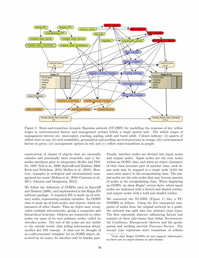
Enough_Bare_Ground

Burn_Decision

Burn_Intensity

Vegetation

Summer_PPTCanal_or_Center

Soil_Type

BurnEffect_on_Willow

Spring_PPTMech_Clearing

GrowingSeason_PPT

Available_Water_Spring Available_Water_Survival

Available_Water_GrowingSeasAvailable_Water_Germination

Level of Cover 0T.

Stage (T)UnoccupiedYearlingSaplingAdultBurnt

2IDI2IDI2IDI2IDI2IDI

Proportion_Germinating Seedling_Survival_Proportion

Level of Cover 0T11.

Stage (T+1)UnoccupiedYearlingSaplingAdultBurnt

2IDI2IDI2IDI2IDI2IDI

Seed_Availability NumberGerminating NumberSurviving

Rooted_Basal_Stem_Diameter 0T.

Rooted_Basal_Stem_Diameter 0T11.

Sapling_Transition

Yearling_Transition

UnOccupied_Transition

Burnt_Adult_Transition

NonInterv_Yearling_Transition

Adult_Transition

Seed_Production

Figure 1: State-and-transition dynamic Bayesian network (ST-DBN) for modelling the response of key willowstages to environmental factors and management actions within a single spatial unit. The willow stages ofmanagement interest are: unoccupied, yearling, sapling, adult and burnt adult. Colours indicate: (i) aspects ofwillow state in tan; (ii) seed availability, germination and seedling survival processes in orange; (iii) environmentalfactors in green; (iv) management options in red; and (v) willow state-transitions in purple.

construction of classes of objects that are internallycohesive and potentially more reuseable, and c) for-malise interfaces prior to integration (Koller and Pfef-fer, 1997; Neil et al., 2000; Kjærulff and Madsen, 2008;Korb and Nicholson, 2010; Molina et al., 2010). How-ever, examples in ecological and environmental man-agement are scant (Molina et al., 2010; Carmona et al.,2011; Johnson and Mengersen, 2012).

We follow the definition of OOBNs used in Kjærulffand Madsen (2008), and implemented in the Hugin BNsoftware package. A standard BN is made up of ordi-nary nodes, representing random variables. An OOBNclass is made up of both nodes, and objects, which areinstances of other classes. Thus an object may encap-sulate multiple sub-networks, giving a composite andhierarchical structure. Objects are connected to othernodes via some of its own ordinary nodes, called itsinterface nodes. The rest of the nodes are not visibleto the outside world, thus hiding information detail,another key OO concept. A class can be thought ofas a self-contained ‘template’ for an OOBN object, de-scribed by its name, its interface and its hidden part.

Finally, interface nodes are divided into input nodesand output nodes. Input nodes are the root nodeswithin an OOBN class, and when an object (instance)of that class becomes part of another class, each in-put node may be mapped to a single node (with thesame state space) in the encapsulating class. The out-put nodes are the only nodes that may become parentsof nodes in the encapsulating class. When displayingan OOBN, we show Hugin1 screen shots, where inputnodes are indicated with a dotted and shaded outline,and output nodes with a bold and shaded outline.

We converted the ST-DBN (Figure 1) into a ST-OODBN as follows. Using the five conceptual cate-gories of nodes from the original network as a guide,the network was split into two abstract class types.The first represents abstract influencing factors andconsists of three sub-classes that define Environmen-tal Conditions, Management Options and the germi-nation and seedling survival Processes Factors. Thesecond type represents state transitions of willows

1Note that Hugin OOBNs do not support inheritance,so there are no super-classes or sub-classes.

79

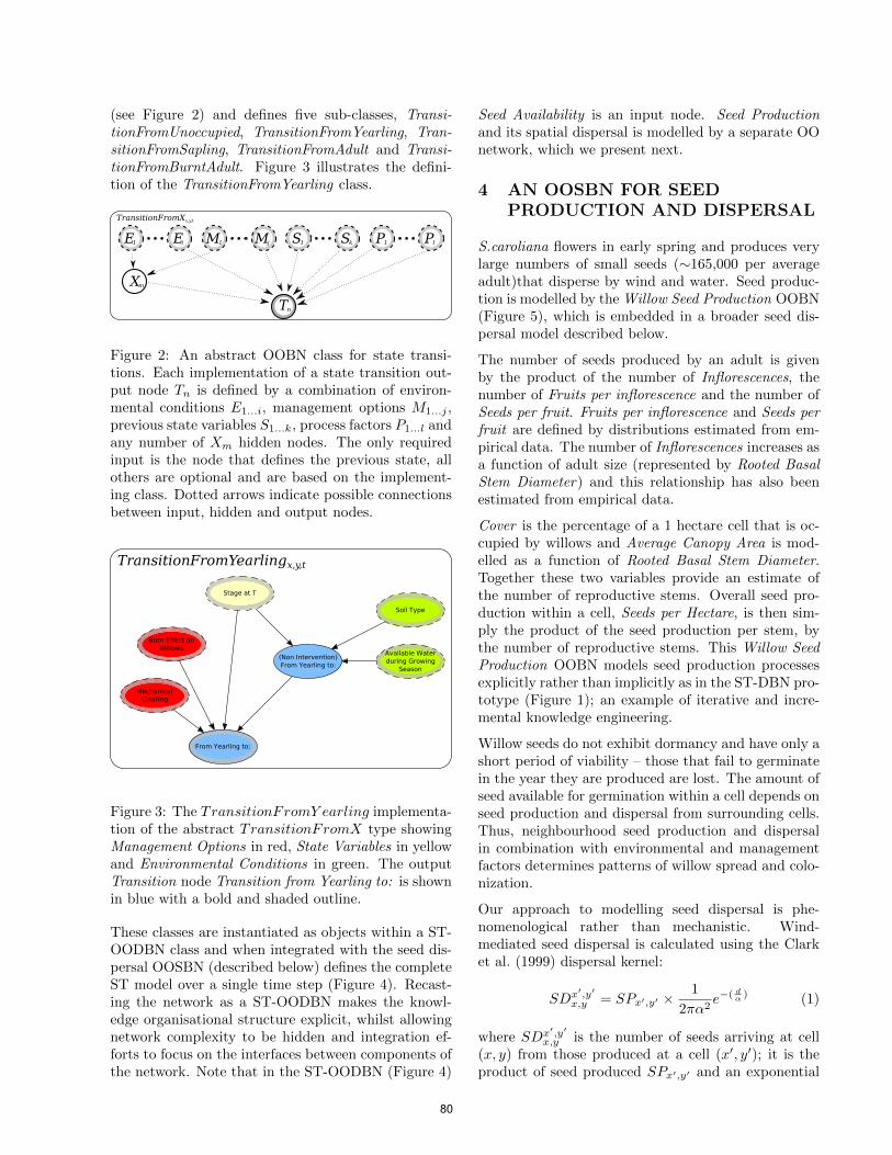
(see Figure 2) and defines five sub-classes, Transi-tionFromUnoccupied, TransitionFromYearling, Tran-sitionFromSapling, TransitionFromAdult and Transi-tionFromBurntAdult. Figure 3 illustrates the defini-tion of the TransitionFromYearling class.

E1 Ei M1 Mj

Tn

TransitionFromXx,y,t

Xm

S1 Sk P1 Pl

Figure 2: An abstract OOBN class for state transi-tions. Each implementation of a state transition out-put node Tn is defined by a combination of environ-mental conditions E1...i, management options M1...j ,previous state variables S1...k, process factors P1...l andany number of Xm hidden nodes. The only requiredinput is the node that defines the previous state, allothers are optional and are based on the implement-ing class. Dotted arrows indicate possible connectionsbetween input, hidden and output nodes.

TransitionFromYearlingx,y,t

Figure 3: The TransitionFromY earling implementa-tion of the abstract TransitionFromX type showingManagement Options in red, State Variables in yellowand Environmental Conditions in green. The outputTransition node Transition from Yearling to: is shownin blue with a bold and shaded outline.

These classes are instantiated as objects within a ST-OODBN class and when integrated with the seed dis-persal OOSBN (described below) defines the completeST model over a single time step (Figure 4). Recast-ing the network as a ST-OODBN makes the knowl-edge organisational structure explicit, whilst allowingnetwork complexity to be hidden and integration ef-forts to focus on the interfaces between components ofthe network. Note that in the ST-OODBN (Figure 4)

Seed Availability is an input node. Seed Productionand its spatial dispersal is modelled by a separate OOnetwork, which we present next.

4 AN OOSBN FOR SEEDPRODUCTION AND DISPERSAL

S.caroliana flowers in early spring and produces verylarge numbers of small seeds (∼165,000 per averageadult)that disperse by wind and water. Seed produc-tion is modelled by the Willow Seed Production OOBN(Figure 5), which is embedded in a broader seed dis-persal model described below.

The number of seeds produced by an adult is givenby the product of the number of Inflorescences, thenumber of Fruits per inflorescence and the number ofSeeds per fruit. Fruits per inflorescence and Seeds perfruit are defined by distributions estimated from em-pirical data. The number of Inflorescences increases asa function of adult size (represented by Rooted BasalStem Diameter) and this relationship has also beenestimated from empirical data.

Cover is the percentage of a 1 hectare cell that is oc-cupied by willows and Average Canopy Area is mod-elled as a function of Rooted Basal Stem Diameter.Together these two variables provide an estimate ofthe number of reproductive stems. Overall seed pro-duction within a cell, Seeds per Hectare, is then sim-ply the product of the seed production per stem, bythe number of reproductive stems. This Willow SeedProduction OOBN models seed production processesexplicitly rather than implicitly as in the ST-DBN pro-totype (Figure 1); an example of iterative and incre-mental knowledge engineering.

Willow seeds do not exhibit dormancy and have only ashort period of viability – those that fail to germinatein the year they are produced are lost. The amount ofseed available for germination within a cell depends onseed production and dispersal from surrounding cells.Thus, neighbourhood seed production and dispersalin combination with environmental and managementfactors determines patterns of willow spread and colo-nization.

Our approach to modelling seed dispersal is phe-nomenological rather than mechanistic. Wind-mediated seed dispersal is calculated using the Clarket al. (1999) dispersal kernel:

SDx′,y′

x,y = SPx′,y′ × 1

2πα2e−(

dα ) (1)

where SDx′,y′

x,y is the number of seeds arriving at cell(x, y) from those produced at a cell (x′, y′); it is theproduct of seed produced SPx′,y′ and an exponential

80

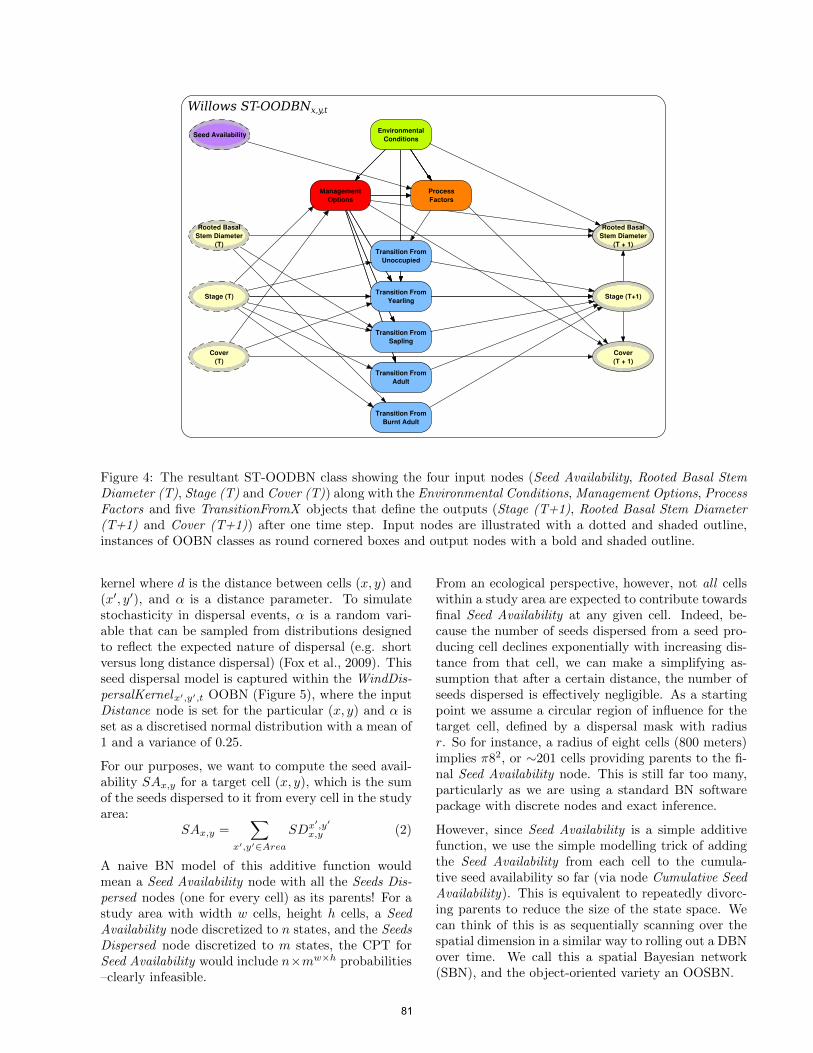
Willows ST-OODBNx,y,t

Figure 4: The resultant ST-OODBN class showing the four input nodes (Seed Availability, Rooted Basal StemDiameter (T), Stage (T) and Cover (T)) along with the Environmental Conditions, Management Options, ProcessFactors and five TransitionFromX objects that define the outputs (Stage (T+1), Rooted Basal Stem Diameter(T+1) and Cover (T+1)) after one time step. Input nodes are illustrated with a dotted and shaded outline,instances of OOBN classes as round cornered boxes and output nodes with a bold and shaded outline.

kernel where d is the distance between cells (x, y) and(x′, y′), and α is a distance parameter. To simulatestochasticity in dispersal events, α is a random vari-able that can be sampled from distributions designedto reflect the expected nature of dispersal (e.g. shortversus long distance dispersal) (Fox et al., 2009). Thisseed dispersal model is captured within the WindDis-persalKernelx′,y′,t OOBN (Figure 5), where the inputDistance node is set for the particular (x, y) and α isset as a discretised normal distribution with a mean of1 and a variance of 0.25.

For our purposes, we want to compute the seed avail-ability SAx,y for a target cell (x, y), which is the sumof the seeds dispersed to it from every cell in the studyarea:

SAx,y =∑

x′,y′∈Area

SDx′,y′

x,y (2)

A naive BN model of this additive function wouldmean a Seed Availability node with all the Seeds Dis-persed nodes (one for every cell) as its parents! For astudy area with width w cells, height h cells, a SeedAvailability node discretized to n states, and the SeedsDispersed node discretized to m states, the CPT forSeed Availability would include n×mw×h probabilities–clearly infeasible.

From an ecological perspective, however, not all cellswithin a study area are expected to contribute towardsfinal Seed Availability at any given cell. Indeed, be-cause the number of seeds dispersed from a seed pro-ducing cell declines exponentially with increasing dis-tance from that cell, we can make a simplifying as-sumption that after a certain distance, the number ofseeds dispersed is effectively negligible. As a startingpoint we assume a circular region of influence for thetarget cell, defined by a dispersal mask with radiusr. So for instance, a radius of eight cells (800 meters)implies π82, or ∼201 cells providing parents to the fi-nal Seed Availability node. This is still far too many,particularly as we are using a standard BN softwarepackage with discrete nodes and exact inference.

However, since Seed Availability is a simple additivefunction, we use the simple modelling trick of addingthe Seed Availability from each cell to the cumula-tive seed availability so far (via node Cumulative SeedAvailability). This is equivalent to repeatedly divorc-ing parents to reduce the size of the state space. Wecan think of this is as sequentially scanning over thespatial dimension in a similar way to rolling out a DBNover time. We call this a spatial Bayesian network(SBN), and the object-oriented variety an OOSBN.

81

SeedDispersal OOSBNt

WillowSeedProductionx'+n,y'+n,t

WindDispersalKernelx'+n,y'+n,t SeedAvailabilityx,y,t

TotalSeedAvailabilityx,y,t

TotalSeedAvailabilityx',y',t

TotalSeedAvailabilityx'+1,y'+1,t

TotalSeedAvailabilityx+n-1,y+n-1,t

Figure 5: The OOSBN architecture showing how Cover, Rooted Basal Stem Diameter, Cumulative Seed Avail-ability and Distance at locations (x′, y′) to (x′+n, y′+n) are combined to provide total seed availability for eachcell at location (x, y) at time t. Dashed arcs indicate that nodes are connected via the seed availability PTLayer.Multiple TotalSeedAvailability objects are illustrated within the SeedDispersal OOSBN reflecting that the totalseeds available at a given (x, y) is dependant on seeds being produced in multiple locations. These syntheticTotalSeedAvailabilty objects are shown as collapsed objects, hiding their private nodes, and showing just thefour input nodes that define the seeds dispersed from each producing cell to the target cell.

Our approach to integrating the seed dispersal makesuse of such an OOSBN, that is run πr2 times (i.e. oncefor every cell (x′, y′) within dispersal range) for eachcell (x, y) in the study area to disperse and then sumthe seed availability at each cell. The dispersal maskis flexible and can be designed to take on differentshapes to reflect potentially important influences onwind dispersal such wind direction, wind strength andterrain characteristics. However, in the results givenSection 6, we use a radius of eight cells.

Overall, our approach here is to mitigate the problemof large CPT sizes by turning the problem in to oneof computation time. This has the added benefit ofpotentially being able to be computed easily in paralleland thus regaining some computation efficiency.

5 Integrating the ST-OODBN withthe OOSBN

Figure 6 is an abstract representation of the systemarchitecture, specifically, the interactions between theGIS layers and the OO networks as the tool is used forprediction at yearly intervals over the required man-agement time frame.

For each cell in the GIS, there is conceptually onestate-transition network (ST-OODBN ) and one seedproduction and dispersal spatial network, (OOSBN ).In practice, we do not store all these as separate net-works, but rather re-use a single network structure,whose input nodes are re-parameterised for each cell,for each time step.

For the first time step, the system takes GIS data,which represents the initial conditions of the studyarea. These are stored in an internal data structure,PTLayer, that combines the spatial structure of theGIS, with distributions for the (discrete) nodes in thenetworks. PTLayers are used to store and pass thespatially referenced prior distributions of input nodesand posterior distributions of output nodes for boththe OOSBN and ST-OODBN (Figure 6). Each PT-Layer contains a number of fields, one for each of thenode states of the linked input and output nodes. Eachfield stores the probability mass of the correspondingnode state.

The PTLayer distributions are used to set the pri-ors for the input nodes at each time step t. Then in-ference (belief updating) is performed within the OOnetwork, producing new posterior probability distri-

82

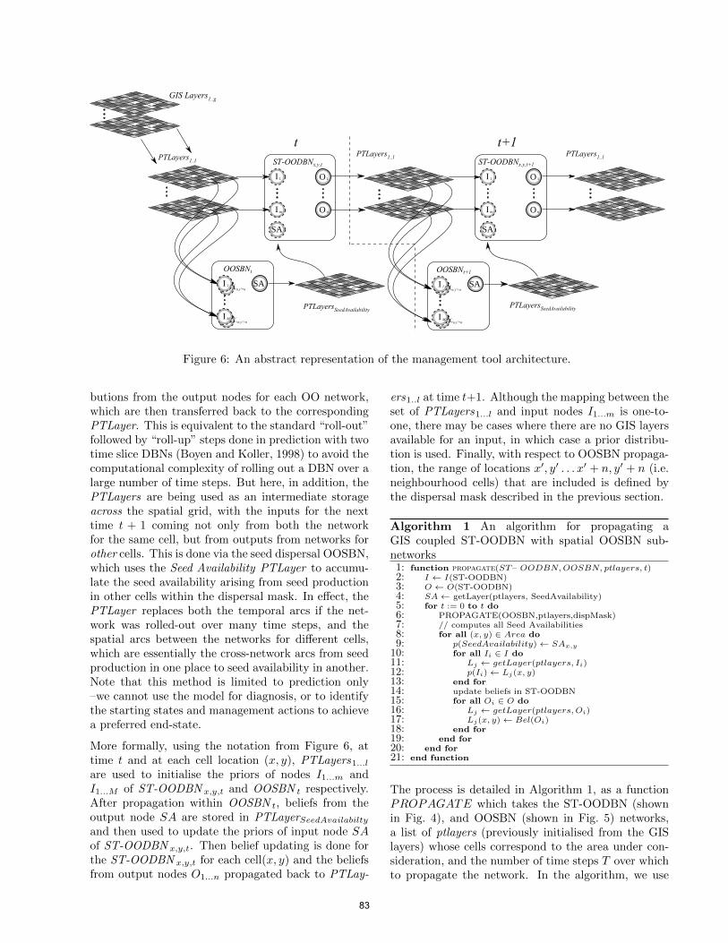
I M,x'+n,y'+n

I 1,x'+n,y'+n

OOSBNt

I 1,x',y'

I M,x',y'

SA

I M,x'+n,y'+n

I 1,x'+n,y'+n

ST-OODBNx,y,t

O 1I 1

I m O n

SA

ST-OODBNx,y,t+1

O 1I 1

I m O n

SA

OOSBNt+1

I 1,x',y'

I M,x',y'

SA

PTLayers1..l

t t+1PTLayers

1..lPTLayers

1..l

GISiLayers1..g

PTLayersSeedAvailability

PTLayersSeedAvailability

Figure 6: An abstract representation of the management tool architecture.

butions from the output nodes for each OO network,which are then transferred back to the correspondingPTLayer. This is equivalent to the standard “roll-out”followed by “roll-up” steps done in prediction with twotime slice DBNs (Boyen and Koller, 1998) to avoid thecomputational complexity of rolling out a DBN over alarge number of time steps. But here, in addition, thePTLayers are being used as an intermediate storageacross the spatial grid, with the inputs for the nexttime t + 1 coming not only from both the networkfor the same cell, but from outputs from networks forother cells. This is done via the seed dispersal OOSBN,which uses the Seed Availability PTLayer to accumu-late the seed availability arising from seed productionin other cells within the dispersal mask. In effect, thePTLayer replaces both the temporal arcs if the net-work was rolled-out over many time steps, and thespatial arcs between the networks for different cells,which are essentially the cross-network arcs from seedproduction in one place to seed availability in another.Note that this method is limited to prediction only–we cannot use the model for diagnosis, or to identifythe starting states and management actions to achievea preferred end-state.

More formally, using the notation from Figure 6, attime t and at each cell location (x, y), PTLayers1...lare used to initialise the priors of nodes I1...m andI1...M of ST-OODBN x,y,t and OOSBN t respectively.After propagation within OOSBN t, beliefs from theoutput node SA are stored in PTLayerSeedAvailabilty

and then used to update the priors of input node SAof ST-OODBN x,y,t. Then belief updating is done forthe ST-OODBN x,y,t for each cell(x, y) and the beliefsfrom output nodes O1...n propagated back to PTLay-

ers1..l at time t+1. Although the mapping between theset of PTLayers1...l and input nodes I1...m is one-to-one, there may be cases where there are no GIS layersavailable for an input, in which case a prior distribu-tion is used. Finally, with respect to OOSBN propaga-tion, the range of locations x′, y′ . . . x′ + n, y′ + n (i.e.neighbourhood cells) that are included is defined bythe dispersal mask described in the previous section.

Algorithm 1 An algorithm for propagating aGIS coupled ST-OODBN with spatial OOSBN sub-networks1: function propagate(ST– OODBN,OOSBN, ptlayers, t)2: I ← I(ST-OODBN)3: O ← O(ST-OODBN)4: SA← getLayer(ptlayers, SeedAvailability)5: for t := 0 to t do6: PROPAGATE(OOSBN,ptlayers,dispMask)7: // computes all Seed Availabilities8: for all (x, y) ∈ Area do9: p(SeedAvailability)← SAx,y

10: for all Ii ∈ I do11: Lj ← getLayer(ptlayers, Ii)12: p(Ii)← Lj(x, y)13: end for14: update beliefs in ST-OODBN15: for all Oi ∈ O do16: Lj ← getLayer(ptlayers,Oi)17: Lj(x, y)← Bel(Oi)18: end for19: end for20: end for21: end function

The process is detailed in Algorithm 1, as a functionPROPAGATE which takes the ST-OODBN (shownin Fig. 4), and OOSBN (shown in Fig. 5) networks,a list of ptlayers (previously initialised from the GISlayers) whose cells correspond to the area under con-sideration, and the number of time steps T over whichto propagate the network. In the algorithm, we use

83

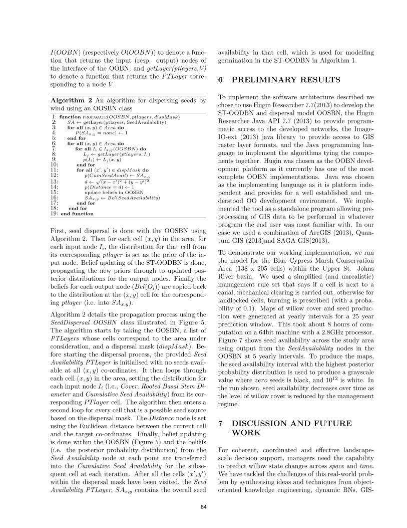
I(OOBN) (respectively O(OOBN)) to denote a func-tion that returns the input (resp. output) nodes ofthe interface of the OOBN, and getLayer(ptlayers,V)to denote a function that returns the PTLayer corre-sponding to a node V .

Algorithm 2 An algorithm for dispersing seeds bywind using an OOSBN class1: function propagate(OOSBN, ptlayers, dispMask)2: SA← getLayer(ptlayers, SeedAvailability)3: for all (x, y) ∈ Area do4: P (SAx,y = none)← 15: end for6: for all (x, y) ∈ Area do7: for all Ii ∈ Ix,y(OOSBN) do8: Lj ← getLayer(ptlayers, Ii)9: p(Ii)← Lj(x, y)10: end for11: for all (x′, y′) ∈ dispMask do12: p(CumSeedAvail)← SAx,y13: d←

√(x− x′)2 + (y − y′)2

14: p(Distance = d)← 115: update beliefs in OOSBN16: SAx,y ← Bel(SeedAvailability)17: end for18: end for19: end function

First, seed dispersal is done with the OOSBN usingAlgorithm 2. Then for each cell (x, y) in the area, foreach input node Ii, the distribution for that cell fromits corresponding ptlayer is set as the prior of the in-put node. Belief updating of the ST-OODBN is done,propagating the new priors through to updated pos-terior distributions for the output nodes. Finally thebeliefs for each output node (Bel(Oi)) are copied backto the distribution at the (x, y) cell for the correspond-ing ptlayer (i.e. into SAx,y).

Algorithm 2 details the propagation process using theSeedDispersal OOSBN class illustrated in Figure 5.The algorithm starts by taking the OOSBN, a list ofPTLayers whose cells correspond to the area underconsideration, and a dispersal mask (dispMask). Be-fore starting the dispersal process, the provided SeedAvailability PTLayer is initialised with no seeds avail-able at all (x, y) co-ordinates. It then loops througheach cell (x, y) in the area, setting the distribution foreach input node Ii (i.e., Cover, Rooted Basal Stem Di-ameter and Cumulative Seed Availability) from its cor-responding PT layer cell. The algorithm then enters asecond loop for every cell that is a possible seed sourcebased on the dispersal mask. The Distance node is setusing the Euclidean distance between the current celland the target co-ordinates. Finally, belief updatingis done within the OOSBN (Figure 5) and the beliefs(i.e. the posterior probability distribution) from theSeed Availability node at each point are transferredinto the Cumulative Seed Availability for the subse-quent cell at each iteration. After all the cells (x′, y′)within the dispersal mask have been visited, the SeedAvailability PTLayer, SAx,y contains the overall seed

availability in that cell, which is used for modellinggermination in the ST-OODBN in Algorithm 1.

6 PRELIMINARY RESULTS

To implement the software architecture described wechose to use Hugin Researcher 7.7(2013) to develop theST-OODBN and dispersal model OOSBN, the HuginResearcher Java API 7.7 (2013) to provide program-matic access to the developed networks, the Image-IO-ext (2013) java library to provide access to GISraster layer formats, and the Java programming lan-guage to implement the algorithms tying the compo-nents together. Hugin was chosen as the OOBN devel-opment platform as it currently has one of the mostcomplete OOBN implementations. Java was chosenas the implementing language as it is platform inde-pendent and provides for a well established and un-derstood OO development environment. We imple-mented the tool as a standalone program allowing pre-processing of GIS data to be performed in whateverprogram the end user was most familiar with. In ourcase we used a combination of ArcGIS (2013), Quan-tum GIS (2013)and SAGA GIS(2013).

To demonstrate our working implementation, we ranthe model for the Blue Cypress Marsh ConservationArea (138 x 205 cells) within the Upper St. JohnsRiver basin. We used a simplified (and unrealistic)management rule set that says if a cell is next to acanal, mechanical clearing is carried out, otherwise forlandlocked cells, burning is prescribed (with a proba-bility of 0.1). Maps of willow cover and seed produc-tion were generated at yearly intervals for a 25 yearprediction window. This took about 8 hours of com-putation on a 64bit machine with a 2.8GHz processor.Figure 7 shows seed availability across the study areausing output from the SeedAvailability nodes in theOOSBN at 5 yearly intervals. To produce the maps,the seed availability interval with the highest posteriorprobability distribution is used to produce a grayscalevalue where zero seeds is black, and 1012 is white. Inthe run shown, seed availability decreases over time asthe level of willow cover is reduced by the managementregime.

7 DISCUSSION AND FUTUREWORK

For coherent, coordinated and effective landscape-scale decision support, managers need the capabilityto predict willow state changes across space and time.We have tackled the challenges of this real-world prob-lem by synthesising ideas and techniques from object-oriented knowledge engineering, dynamic BNs, GIS-

84

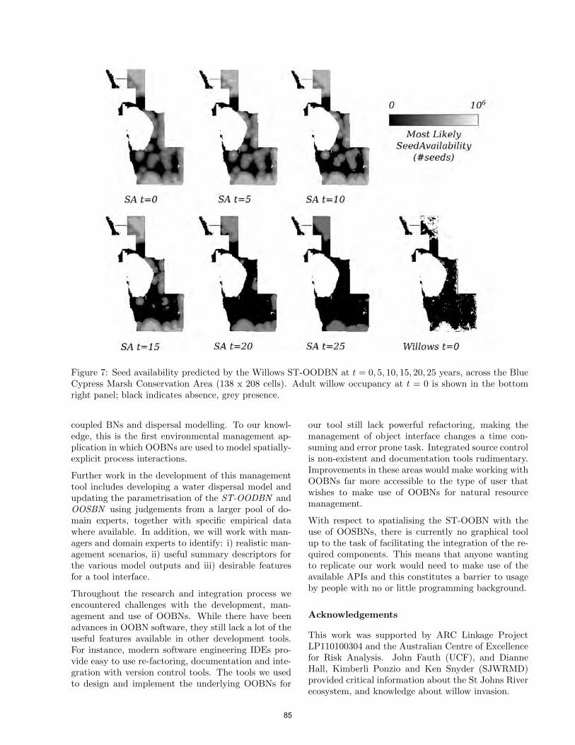
Figure 7: Seed availability predicted by the Willows ST-OODBN at t = 0, 5, 10, 15, 20, 25 years, across the BlueCypress Marsh Conservation Area (138 x 208 cells). Adult willow occupancy at t = 0 is shown in the bottomright panel; black indicates absence, grey presence.

coupled BNs and dispersal modelling. To our knowl-edge, this is the first environmental management ap-plication in which OOBNs are used to model spatially-explicit process interactions.

Further work in the development of this managementtool includes developing a water dispersal model andupdating the parametrisation of the ST-OODBN andOOSBN using judgements from a larger pool of do-main experts, together with specific empirical datawhere available. In addition, we will work with man-agers and domain experts to identify: i) realistic man-agement scenarios, ii) useful summary descriptors forthe various model outputs and iii) desirable featuresfor a tool interface.

Throughout the research and integration process weencountered challenges with the development, man-agement and use of OOBNs. While there have beenadvances in OOBN software, they still lack a lot of theuseful features available in other development tools.For instance, modern software engineering IDEs pro-vide easy to use re-factoring, documentation and inte-gration with version control tools. The tools we usedto design and implement the underlying OOBNs for

our tool still lack powerful refactoring, making themanagement of object interface changes a time con-suming and error prone task. Integrated source controlis non-existent and documentation tools rudimentary.Improvements in these areas would make working withOOBNs far more accessible to the type of user thatwishes to make use of OOBNs for natural resourcemanagement.

With respect to spatialising the ST-OOBN with theuse of OOSBNs, there is currently no graphical toolup to the task of facilitating the integration of the re-quired components. This means that anyone wantingto replicate our work would need to make use of theavailable APIs and this constitutes a barrier to usageby people with no or little programming background.

Acknowledgements

This work was supported by ARC Linkage ProjectLP110100304 and the Australian Centre of Excellencefor Risk Analysis. John Fauth (UCF), and DianneHall, Kimberli Ponzio and Ken Snyder (SJWRMD)provided critical information about the St Johns Riverecosystem, and knowledge about willow invasion.

85

References

Bashari, H., Smith, C., and Bosch, O. (2009). De-veloping decision support tools for rangeland man-agement by combining state and transition modelsand Bayesian belief networks. Agricultural Systems,99(1):23–34.

Bestelmeyer, B. T., Brown, J. R., Havstad, K. M.,Alexander, R., Chavez, G., and Herrick, J. E.(2003). Development and use of state-and-transitionmodels for rangelands. Journal of Range Manage-ment, (2):114–126.

Boyen, X. and Koller, D. (1998). Tractable inferencefor complex stochastic processes. In Proceedings ofthe Fourteenth Conference on Uncertainty in Arti-ficial Intelligence, UAI’98, pages 33–42, San Fran-cisco, CA, USA. Morgan Kaufmann Publishers Inc.

Carmona, G., Molina, J., and Bromley, J. (2011).Object-Oriented Bayesian networks for participa-tory water management: two case studies in Spain.Journal of Water Resources Planning and Manage-ment, 137(4):366–376.

Clark, J. D., Silman, M., Kern, R., Macklin, E., andHille Ris Lambers, J. (1999). Seed dispersal near andfar: patterns across temperate and tropical forests.Ecology, 80(5):1475–1494.

Dean, T. and Kanazawa, K. (1989). A model for rea-soning about persistence and causation. Computa-tional Intelligence, 5:142–150.

Esri (2013). ArcGIS (Version 10.1) [Software].http://www.esri.com/software/arcgis.

Fox, J. C., Buckley, Y. M., Panetta, F. D., Bourgoin,J., and Pullar, D. (2009). Surveillance protocols formanagement of invasive plants: modelling Chileanneedle grass (Nassella neesiana) in Australia. Di-versity and Distributions, 15(4):577–589.

GeoSolutions (2013). Image-IO-ext JavaLibrary (Version 1.1.7) [Software].http://github.com/geosolutions-it/.

Hugin Expert A/S (2013). Hugin Researcher (Version7.7) [Software]. http://www.hugin.com.

Johnson, S. and Mengersen, K. (2012). IntegratedBayesian network framework for modeling complexecological issues. Integrated Environmental Assess-ment and Management, 8(3):480–90.

Kinser, P., Lee, M. A., Dambek, G., Williams, M.,Ponzio, K., and Adamus, C. (1997). Expansionof Willow in the Blue Cypress Marsh ConservationArea, Upper St. Johns River Basin. Technical re-port, St. Johns River Water Management District,Palatka, Florida.

Kjærulff, U. B. and Madsen, A. (2008). Bayesian Net-works and Influence Diagrams: A Guide to Con-struction and Analysis. Springer Verlag, New York.

Koller, D. and Pfeffer, A. (1997). Object-orientedBayesian networks. In Proceedings of the Thirteenth

Conference on Uncertainty in Artificial Intelligence,UAI’97, pages 302–313, San Francisco, CA, USA.Morgan Kaufmann Publishers Inc.

Korb, K. B. and Nicholson, A. (2010). Bayesian arti-ficial intelligence. Chapman&Hall/CRC, Boca Ra-ton, FL, 2nd edition.

Molina, J., Bromley, J., Garcıa-Arostegui, J., Sulli-van, C., and Benavente, J. (2010). Integrated wa-ter resources management of overexploited hydro-geological systems using Object-Oriented BayesianNetworks. Environmental Modelling & Software,25(4):383–397.

Neil, M., Fenton, N., and Nielson, L. (2000). Build-ing large-scale Bayesian networks. The KnowledgeEngineering Review, 15(3):1–33.

Nicholson, A., Chee, Y., and Quintana-Ascencio, P.(2012). A state-transition DBN for management ofwillows in an american heritage river catchment. InNicholson, A., Agosta, J. M., and Flores, J., edi-tors, Ninth Bayesian Modeling Applications Work-shop at the Conference of Uncertainty in ArtificialIntelligence, Catalina Island, CA, USA, http://ceur-ws.org/Vol-962/paper07.pdf.

Nicholson, A. E. (1992). Monitoring Discrete Environ-ments using Dynamic Belief Networks. PhD thesis,Department of Engineering Sciences, Oxford.

Nicholson, A. E. and Flores, M. J. (2011). Combiningstate and transition models with dynamic Bayesiannetworks. Ecological Modelling, 222(3):555–566.

Quantum GIS Development Team (2013).Quantum GIS (Version 1.8.0) [Software].http://www.qgis.org/.

Quintana-Ascencio, P. F., Fauth, J. E., CastroMorales, L. M., Ponzio, K. J., Hall, D., and Sny-der, K. (2013). Taming the beast: managing hydrol-ogy to control Carolina Willow (Salix caroliniana)seedlings and cuttings. Restoration Ecology.

Rumpff, L., Duncan, D., Vesk, P., Keith, D., and Win-tle, B. (2011). State-and-transition modelling foradaptive management of native woodlands. Biolog-ical Conservation, 144(4):1224–1236.

SAGA Development Team (2013). SAGA GIS (Version2.0.8) [Software]. http://www.saga-gis.org/.

Shihab, K. (2008). Dynamic modeling of groundwaterpollutants with Bayesian networks. Applied Artifi-cial Intelligence, 22(4):352–376.

86

Exploring Multiple Dimensions of Parallelism in Junction TreeMessage Passing

Lu ZhengElectrical and Computer Engineering


Ole J. MengshoelElectrical and Computer Engineering


Abstract

Belief propagation over junction trees isknown to be computationally challenging inthe general case. One way of addressing thiscomputational challenge is to use node-levelparallel computing, and parallelize the com-putation associated with each separator po-tential table cell. However, this approach isnot efficient for junction trees that mainlycontain small separators. In this paper,we analyze this problem, and address it bystudying a new dimension of node-level par-allelism, namely arithmetic parallelism. Inaddition, on the graph level, we use a cliquemerging technique to further adapt junctiontrees to parallel computing platforms. Weapply our parallel approach to both marginaland most probable explanation (MPE) infer-ence in junction trees. In experiments with aGraphics Processing Unit (GPU), we obtainfor marginal inference an average speedupof 5.54x and a maximum speedup of 11.94x;speedups for MPE inference are similar.

1 INTRODUCTION

Bayesian networks (BN) are frequently used to repre-sent and reason about uncertainty. The junction treeis a secondary data structure which can be compiledfrom a BN [2, 4, 5, 9, 10, 19]. Junction trees can beused for both marginal and most probable explanation(MPE) inference in BNs. Sum-product belief propaga-tion on junction tree is perhaps the most popular ex-act marginal inference algorithm [8], and max-productbelief propagation can be used to compute the mostprobable explanations [2, 15]. However, belief propa-gation is computationally hard and the computationaldifficulty increases dramatically with the density of theBN, the number of states of each network node, and

the treewidth of BN, which is upper bounded by thegenerated junction tree [13]. This computational chal-lenge may hinder the application of BNs in cases wherereal-time inference is required.

Parallelization of Bayesian network computation is afeasible way of addressing this computational challenge[1,6,7,9,11,12,14,19,20]. A data parallel implementa-tion for junction tree inference has been developed fora cache-coherent shared-address-space machine withphysically distributed main memory [9]. Parallelismin the basic sum-product computation has been in-vestigated for Graphics Processing Units (GPUs) [19].The efficiency in using disk memory for exact infer-ence, using parallelism and other techniques, has beenimproved [7]. An algorithm for parallel BN inferenceusing pointer jumping has been developed [14]. Bothparallelization based on graph structure [12] as well asnode level primitives for parallel computing based ona table extension idea have been introduced [20]; thisidea was later implemented on a GPU [6]. Gonzalezet al. developed a parallel belief propagation algorithmbased on parallel graph traversal to accelerate the com-putation [3].

A parallel message computation algorithm for junc-tion tree belief propagation, based on the cluster-sepset mapping method [4], has been introduced [22].Cluster-sepset based node level parallelism (denotedelement-wise parallelism in this paper) can acceleratethe junction tree algorithm [22]; unfortunately the per-formance varies substantially between different junc-tion trees. In particular, for small separators in junc-tion trees, element-wise parallelism [22] provides lim-ited parallel opportunity as explained in this paper.

Our work aims at addressing the small separator issue.Specifically, this paper makes these contributions thatfurther speed up computation and make performancemore robust over different BNs from applications:

• We discuss another dimension of parallelism,namely arithmetic parallelism (Section 3.1). Inte-

87

grating arithmetic parallelism with element-wiseparallelism, we develop an improved parallel sum-product propagation algorithm as discussed inSection 3.2.

• We also develop and test a parallel max-product(Section 3.3) propagation algorithm based on thetwo dimensions of parallelism.

• On the graph level, we use a clique merging tech-nique (Section 4), which leverages the two dimen-sions of parallelism, to adapt the various Bayesiannetworks to the parallel computing platform.

In our GPU experiments, we test the novel two-dimensional parallel approach for both regular sum-propagation and max-propagation. Results show thatour algorithms improve the performance of both kindsof belief propagation significantly.

Our paper is organized as follows: In Section 2, wereview BNs, junction trees parallel computing usingGPUs, and the small-separator problem. In Section3 and Section 4, we describe our parallel approach tomessage computation for belief propagation in junc-tion trees. Theoretical analysis of our approach is inSection 5. Experimental results are discussed in Sec-tion 6, while Section 7 concludes and outlines futureresearch.

2 BACKGROUND

2.1 Belief Propagation in Junction Trees

A BN is a compact representation of a joint distribu-tion over a set of random variables X . A BN is struc-tured as a directed acyclic graph (DAG) whose verticesare the random variables. The directed edges inducedependence and independence relationships among therandom variables. The evidence in a Bayesian networkconsists of instantiated random variables.

The junction tree algorithm propagates beliefs (or pos-teriors) over a derived graph called a junction tree. Ajunction tree is generated from a BN by means of mor-alization and triangulation [10]. Each vertex Ci of thejunction tree contains a subset of the random variablesand forms a clique in the moralized and triangulatedBN, denoted by Xi ⊆ X . Each vertex of the junctiontree has a potential table φXi

. With the above nota-tions, a junction tree can be defined as J = (T,Φ),where T represents a tree and Φ represents all the po-tential tables associated with this tree. Assuming Ciand Cj are adjacent, a separator Sij is induced on aconnecting edge. The variables contained in Sij aredefined to be Xi ∩ Xj .

The junction tree size, and hence also junction treecomputation, can be lower bounded by treewidth,which is defined to be the minimal size of the largestjunction tree clique minus one. Considering a junctiontree with a treewidth tw, the amount of computation islower-bounded by O(exp(c∗tw)) where c is a constant.

Belief propagation is invoked when we get new evi-dence e for a set of variables E ⊆ X . We need to up-date the potential tables Φ to reflect this new informa-tion. To do this, belief propagation over the junctiontree is used. This is a two-phase procedure: evidencecollection and evidence distribution. For the evidencecollection phase, messages are collected from the leafvertices all the way up to a designated root vertex.For the evidence distribution phase, messages are dis-tributed from the root vertex to the leaf vertices.

2.2 Junction Trees and Parallelism

Current emerging many-core platforms, like the recentGraphical Processing Units (GPUs) from NVIDIA andIntel’s Knights Ferry, are built around an array of pro-cessors running many threads of execution in parallel.These chips employ a Single Instruction Multiple Data(SIMD) architecture. Threads are grouped using aSIMD structure and each group shares a multithreadedinstruction unit. The key to good performance on suchplatforms is finding enough parallel opportunities.

We now consider opportunities for parallel computingin junction trees. Associated with each junction treevertex Ci and its variables Xi, there is a potential ta-ble φXi containing non-negative real numbers that areproportional to the joint distribution of Xi. If eachvariable contains sj states, the minimal size of the

potential table is |φXi| =

∏|Xi|j=1 sj , where |Xi| is the

cardinality of Xi.

Message passing from Ci to an adjacent vertex Ck, withseparator Sik, involves two steps:

1. Reduction step. In sum-propagation, the po-tential table φSik of the separator is updated toφ∗Sik by reducing the potential table φXi :

φ∗Sik =∑Xi/Sik

φXi. (1)

2. Scattering step. The potential table of Ck isupdated using both the old and new table of Sik:

φ∗Xk= φXk

φ∗SikφSik

. (2)

We define 00 = 0 in this case, that is, if the de-

nominator in (2) is zero, then we simply set thecorresponding φ∗Xk

to zeros.

88

Figure 1: Histograms of the separator potential tablesizes of junction trees Pigs and Munin3. For both junc-tion trees, the great majority of the separator tablescontain 20 or fewer elements.

Equation (1) and (2) reveal two dimensions of par-allelism opportunity. The first dimension, which wereturn to in Section 3, is arithmetic parallelism. Thesecond dimension is element-wise parallelism [22].

Element-wise parallelism in junction trees is based onthe fact that the computation related to each sepa-rator potential table cell are independent, and takesadvantage of an index mapping table, see Figure 2. InFigure 2, this independence is illustrated by the whiteand grey coloring of cells in the cliques, the separa-tor, and the index mapping tables. More formally, anindex mapping table µX ,S stores the index mappingsfrom φX to φS [4]. We create |φSik | such mappingtables. In each mapping table µXi,φSik (j)

we store theindices of the elements of φXi

mapping to the j-th sep-arator table element. Mathematically,

µXi,φSik (j)= r ∈ [0, |φXi

| − 1] |φXi

(r) is mapped to φSik(j).

With the index mapping table, element-wise paral-lelism is obtained by assigning one thread per map-ping table of a separator potential table as illustratedin Figure 2 and Figure 3. Consequently, belief prop-agation over junction trees can often be sped up byusing a hybrid CPU/GPU approach [22].

2.3 Small Separator Problem

Figure 1 contains the histograms of two real-world BNsPigs and Munin3.1 We see that most separators inthese two BNs are quite small and have a potentialtable size of less than 20.

In general, small separators can be found in these threescenarios: (i) due to two small neighboring cliques (we

1These BNs can be downloaded at http://bndg.cs.aau.dk/html/bayesian_networks.html

Figure 2: Due to the small separator in the B-S-Spattern, a long index mapping table is produced. Ifonly element-wise parallelism is used, there is just onethread per index mapping table, resulting in slow se-quential computation.

call it the S-S-S pattern); (ii) due to a small intersec-tion set of two big neighboring cliques (the B-S-B pat-tern); and (iii) due to one small neighboring clique andone big neighboring clique (the B-S-S pattern).2 Dueto parallel computing issues, detailed next, these threepatterns characterize what we call the small-separatorproblem.

Unfortunately, element-wise parallelism may not pro-vide enough parallel opportunities when a separatoris very small and the mapping tables to one or bothcliques are very long. A small-scale example, reflect-ing the B-S-S pattern, is shown in Figure 2.3 Whilethe mapping tables may be processed in parallel, thelong mapping tables result in a significant amount ofsequential computation within each mapping table.

A state of the art GPU typically supports more thanone thousand concurrent threads, thus message pass-ing through small separators will leave most of theGPU resources idle. This is a major bottleneck for theperformance, which we address next.

In this paper, to handle the small separator problem,we use clique merging to eliminate small separators(see Section 4) resulting from the S-S-S pattern andarithmetic parallelism (see Section 3) to attack the B-

2These patterns, when read left-to-right, describe thesize of a clique, the size of a neigboring separator, andthe size of a neigboring clique (different from the first) asfound in a junction tree. For example, the pattern B-S-Sdescribes a big clique, a small separator, and a small clique.

3In fact, both the “long” and “short” index mappingtables have for presentation purposes been made short–ina realistic junction tree a “long” table can have more than10,000 entries.

89

Figure 3: Example of data structure for two GPUcliques and their separator. Arithmetic parallelism(the reverse pyramid at the bottom) is integrated withelement-wise parallelism (mapping tables at the top).The arithmetic parallelism achieves parallel summa-tion of 2d terms in d cycles.

S-S and B-S-B patterns.

3 PARALLEL MESSAGE PASSINGIN JUNCTION TREES

In order to handle the small-separator problem, wediscuss another dimension of parallelism in additionto element-wise parallelism, namely arithmetic paral-lelism. Arithmetic parallelim explores the parallel op-portunity in the sum of (1) and in the multiplicationof (2). By considering also arithmetic parallelism, wecan better match the junction tree and the many-coreGPU platform by optimizing the computing resourcesallocated to the two dimensions of parallelism.

Mathematically, this optimization can be modeled asa computation time minimization problem:

minpe,pa T (pe, pa, Ci, Cj ,Φ),subject to : pe + pa ≤ ptot

(3)

where T (·) is the time consumed for a message pass-ing from clique Ci to clique Cj ; pe and pa are the num-ber of parallel threads allocated to the element-wiseand arithmetic dimensions respectively; ptot is the to-tal number of parallel threads available in the GPU;and Φ is a collection of GPU-related parameters, suchas the cache size, etc. Equation (3) is a formulation ofoptimizing algorithm performance on a parallel com-puting platform. Unfortunately, traditional optimiza-tion techniques can typically not be applied to thisoptimization problem. This is because the analyticalform of T (·) is usually not available, due to the com-plexity of the hardware platform. So in our work wechoose pe and pa empirically for our implementation.

In the rest of this section, we will describe our algo-rithm design, seeking to explore both element-wise andarithmetic parallelism.

3.1 Arithmetic Parallelism

Arithmetic parallelism needs to be explored in differentways for reduction and scattering, and also integratedwith element-wise parallelism, as we will discuss now.

For reduction, given a certain fixed element j, Equa-tion (1) is essentially a summation over all the cliquepotential table φXi elements indicated by the corre-sponding mapping table µXi,φSik (j)

. The number of

sums is |µXi,φSik (j)|. We compute the summation in

parallel by using the approach illustrated in Figure 3.This improves the handling of long index mapping ta-bles induced, for example, by the B-S-B and B-S-Spatterns. The summation is done in several iterations.In each iteration, the numbers are divided into twogroups and the corresponding two numbers in each

90

group are added in parallel. At the end of this recur-sive process, the sum is obtained, as shown in Algo-rithm 1. The input parameter d is discussed in Section3.2; the remaining inputs are an array of floats.

Algorithm 1 ParAdd(d, op(0), . . . , op(2d − 1))

Input: d, op(0), . . . , op(2d − 1).sum = 0for i = 1 to d dofor j = 0 to 2d−i − 1 in parallel doop(j) = op(j) + op(j + 2d−i)

end forend forreturn op(0)

For scattering, Equation (2) updates the elementsof φXk

independently despite that φSik and φ∗Sik arere-used to update different elements. Therefore, wecan compute each multiplication in (2) with a singlethread. The parallel multiplication algorithm is givenin Algorithm 2. The input parameter p is discussedin Section 3.2; the remaining inputs are an array offloats.

Algorithm 2 ParMul(p, op1, op2(0), . . . , op2(p− 1))

Input: p, op1, op2(0), . . . , op2(p− 1).sum = 0for j = 0 to p− 1 in parallel doop2(j) = op1 ∗ op2(j)

end for

3.2 Parallel Belief Propagation

Combining element-wise and arithmetic parallelism,we design the reduction and scattering operations asshown in Algorithm 3 and Algorithm 4. Both of thesealgorithms take advantage of arithmetic parallelism.In Algorithm 3, the parameter d is the number of cy-cles used to compute the reduction (summation), whilein Algorithm 4, p is the number of threads operatingin parallel. Both p and d are parameters that deter-mine the degree of arithmetic parallelism. They canbe viewed as a special form of pa in (3). Based onAlgorithm 3 and Algorithm 4, junction tree messagepassing can be written as shown in Algorithm 5.

Belief propagation can be done using both breadth-first and depth-first traversal over a junction tree. Weuse the Hugin algorithm [5], which adopts depth-firstbelief propagation. Given a junction tree J with rootvertex Croot, we first initialize the junction tree bymultiplying together the Bayesian network potentialtables (CPTs). Then, two phase belief propagationis adopted [10]: collect evidence and then distributeevidence [22].

Algorithm 3 Reduction(d, φXi , φSik , µXi,Sik)

Input: d, φXi, φSik , µXi,Sik .

for n = 1 to |φSik | in parallel dofor j = 0 to d|µXi,Sik(n)|/2de do

sum = sum + ParAdd(d, φXi(µXi,Sik(n)(j ∗

2d)), . . . , φXi(µXi,Sik(n)((j + 1) ∗ 2d − 1)))

end forend for

Algorithm 4 Scattering(p, φXk, φSik , µXk,Sik)

Input: p, φXk, φSik , µXk,Sik .

for n = 1 to |φSik | in parallel dofor j = 0 to d|φSik |/pe do

sum = sum +

ParMul(p,φ∗Sik

(n)

φSik (n), φXk

(µXk,Sik(n)(j ∗p)), . . . , φXk

(µXk,Sik(n)((j + 1) ∗ p− 1)))end for

end for

3.3 Max-product Belief Propagation

In this paper, we also apply our parallel tech-niques to max-product propagation (or in short, max-propagation), which is also referred as the Viterbialgorithm. Max-propagation solves the problem ofcomputing a most probable explanation. For max-propagation, the

∑in (1) is replaced by max [2,15]. In

this paper we use sum-product propagation to explainour parallel algorithms; the explanation can generallybe changed to discuss max-propagation by replacingadd with max.

4 CLIQUE MERGING FORJUNCTION TREES

The performance of our parallel algorithm is to a largeextent determined by the degree of parallelism avail-able in message passing, which intuitively can be mea-sured by the separator size |φSik |, which determinesthe element-wise parallelism, and the mapping tablesize |µXi,Sik(n)| which upper bounds the arithmeticparallelism. In other words, the larger |φSik | and|µXi,Sik(n)| are, the greater is the parallelism opportu-nity. Therefore, message passing between small cliques(the S-S-S pattern), where |φSik | and |µXi,Sik(n)| aresmall, is not expected to have good performance.There is not enough parallelism to make full use of

Algorithm 5 PassMessage(p, d, φXi, φXk

, φSik , µXi,Sik)

Input: p, d, φXi , φXk, φSik , µXi,Sik .

Reduction(d, φXi, φSik , µXi,Sik)

Scattering(p, φXk, φSik , µXk,Sik)

91

a GPU’s computing resources.

In order to better use the GPU computing power,we propose to remove small separators (that followthe S-S-S pattern) by selectively merging neighboringcliques. This increases the length of mapping tables,however the arithmetic parallelism techniques intro-duced in Section 3 can handle this. Clique mergingcan be done offline according to this theorem [8].

Theorem 4.1 Two neighboring cliques Ci and Cj ina junction tree J with the separator Sij can be mergedtogether into an equivalent new clique Cij with the po-tential function

φ(xCij ) =φ(xCi

)φ(xCj)

φ(xSij)

, (4)

while keeping all the other part of the junction treeunchanged.

The result of merging cliques is three-fold: (i) it pro-duces larger clique nodes and thus longer mapping ta-bles; (ii) it eliminates small separators; and (iii) it re-duces the number of cliques. Larger clique nodes willresult in more computation and therefore longer pro-cessing time for each single thread, but getting rid ofsmall separators will improve utilization of the GPUand reduce computation time. We have to managethese two conflicting objectives to improve the overallperformance of our parallel junction tree algorithm.

Our algorithm for clique merging is shown in Algo-rithm 6. It uses two heuristic thresholds, the sepa-rator size threshold τs and the index mapping tablesize threshold τµ, to control the above-mentioned twoeffects. We only merge two neighboring cliques Ciand Cj into a new clique Cij when |φSij | < τs and|µXj ,φS

| < τµ.

Algorithm 6 MergeCliques(J , τs, τµ)

merge flag = 1while merge flag do

merge flag = 0for each adjacent clique pair (Ci, Cj) in J doif φS < τs and |µXj ,φS

| < τµ thenMerge (J,Ci, Cj)merge flag = 1

end ifend for

end while

Given an S-S-S-S-S pattern, Algorithm 6 may mergetwo S cliques and produce an S-B-S pattern. Here, Bis the merged clique. Note that the B-S sub-patterncreates a long index mapping table, which is exactlywhat arithmetic parallelism handles. There is in other

words potential synergy between clique merging andarithmetic parallelism, as is further explored in exper-iments in Section 6.

5 ANALYSIS AND DISCUSSION

In this section, we analyze the theoretical speedup forour two-dimensional parallel junction tree inference al-gorithm under the idealized assumption that there isunlimited parallel threads available from the many-core computing platform.

The degree of parallelism opportunity is jointly de-termined by the size of the separators’ potential ta-ble, |φS |, and the size of the index mapping table|µX ,φS

|. Consider a message passed from Ci to Ck.Since we employ separator table element-wise paral-lelism in our algorithm, we only need to focus on thecomputation related to one particular separator tableelement. With the assumption of unlimited parallelthreads, we can choose d = dlog |µXi,φS

|e. The timecomplexity for the reduction is then dlog |µXi,φS

|e, dueto our use of summation parallelism.4 Note since

|µXi,φS| =

|φXi|

|φS | , the time complexity can be written

as dlog |φXi| − log |φS |e. For the scattering phase, we

choose p = |µXk,φS| and the time complexity is given

by |µXk,φS|/p+ 1 = 2 due to the multiplication paral-

lelism. Thus the overall time complexity of the two-dimensional belief propagation algorithm is:

dlog |φXi| − log |φS |e+ 2, (5)

which is the theoretical optimal time complexity un-der the assumption of an infinite number of threads.Nevertheless, this value is hard to achieve in practicesince the value of d and p are subject to the concur-rency limit of the computing platform. For example, inthe above-mentioned BN Pigs, some message passingrequires p = 1120 while the GTX460 GPU supports atmost 1024 threads per thread block.

Belief propagation is a sequence of messages passed ina certain order [10], for both CPU and GPU [22]. LetNe(C) denote the neighbors of C in the junction tree.The time complexity for belief propagation is∑

i

∑k∈Ne(Ci)

(dlog |φXi | − log |φS |e+ 2) ,

Kernel invocation overhead, incurred each time Algo-rithm 5 is invoked, turns out to be an important per-formance factor. If we model the invocation overheadfor each kernel call to be a constant τ , then the time

4We assume, for simplicity, sum-propagation. The anal-ysis for max-propagation is similar.

92

complexity becomes∑i

diτ +∑i

∑k∈Ne(Ci)

(dlog |φXi| − log |φS |e+ 2) ,

where di is the degree of a node Ci. In a tree structure,∑di = 2(n− 1). Thus the GPU time complexity is

2(n− 1)τ +∑i

∑k∈Ne(Ci)

(dlog |φXi | − log |φS |e+ 2) .

From this equation, we can see that the junction treetopology impacts GPU performance in at least twoways: the total invocation overhead is proportional tothe number of nodes in the junction tree, while theseparator and clique table sizes determine the degreeof parallelism.

The overall speedup of our parallel belief propagationapproach is determined by the equation

Speedup =

∑i

∑k∈Ne(Ci)(|φXi

|+ |φXk|)

2(n− 1)τ +∑i

∑k∈Ne(Ci)

(⌈log|φXi|

|φS |

⌉+ 2) .

Clearly, the speedup depends on the distribution ofthe sizes of the separators’ and cliques’ potential ta-bles. That is the reason we propose the clique mergingtechnique. Using clique merging, we change the num-ber of nodes in the junction tree and distribution ofthe size of the separators’ and cliques’ potential ta-ble as well, adapting the junction tree for the specificparallel computing platform.

From the equations above, we can estimate the overallbelief propagation speedup. However, taking into ac-count that the CPU/GPU platform incurs invocationoverhead and the long memory latency when loadingdata from slow device memory to fast shared memory,the theoretical speedup is hard to achieve in practice.We take an experimental approach to study how thestructure of the junction trees affects the performanceof our parallel technique on the CPU/GPU setting inSection 6.

6 EXPERIMENTAL RESULTS

In experiments, we study Bayesian networks compiledinto junction trees. We not only want to comparethe two-dimensional parallel junction tree algorithm tothe sequential algorithm, but also study how effectivethe arithmetic parallelism and clique merging methodsare. Consequently, we experiment with different com-binations of element-wise parallelism (EP), arithmeticparallelism (AP), and clique merging (CM).

6.1 Computing Platform

We use the NVIDIA GeForce GTX460 as the platformfor our implementation. This GPU consists of sevenmultiprocessors, and each multiprocessor consists of48 cores and 48K on-chip shared memory per threadblock. The peak thread level parallelism achieves907GFlop/s. In addition to the fast shared memory,a much larger but slower off-chip global memory (785MB) that is shared by all multiprocessors is provided.The bandwidth between the global and shared mem-ories is about 90 Gbps. In the junction tree compu-tations we are using single precision for the GPU andthe thread block size is set to 256.

6.2 Methods and Data

For the purpose of comparison, we use the same setof BNs as used previously [22] (see http://bndg.cs.

aau.dk/html/bayesian_networks.html). They arefrom different domains, with varying structures andstate spaces. These differences lead to very differ-ent junction trees, see Table 1, resulting in varyingopportunities for element-wise and arithmetic paral-lelism. Thus, we use clique merging to carefully con-trol our two dimensions of parallelism to optimize per-formance. The Bayesian networks are compiled intojunction trees and merged offline and then junctiontree propagation is performed.

6.3 GPU Optimization: ArithmeticParallelism

Arithmetic parallelism gives us more freedom to matchthe parallelism in message passing and the concur-rency provided by a GPU: when there is not enoughpotential table element-wise parallelism available, wecan increase the degree of arithmetic parallelism. Thenumber of threads assigned to arithmetic parallelismaffects the performance significantly. The parameterp in parallel scattering and the parameter 2d in theparallel reduction should be chosen carefully (see Al-gorithm 1 and 2). Since the GPU can provide onlylimited concurrency, we need to balance the arithmeticparallelism and the element-wise parallelism for eachmessage passing to get the best performance.

Consider message passing between big cliques, for ex-ample according to the B-S-B pattern. Intuitively, thevalues of the arithmetic parallelism parameters p andd should be set higher than for the message passingbetween smaller cliques. Thus, based on extensive ex-perimentation, we currently employ a simple heuristicparameter selection scheme for the scattering param-eter p

p =

4 if|µXi,Sik(n)| ≤ 100

128 if|µXi,Sik(n)| > 100(6)

93

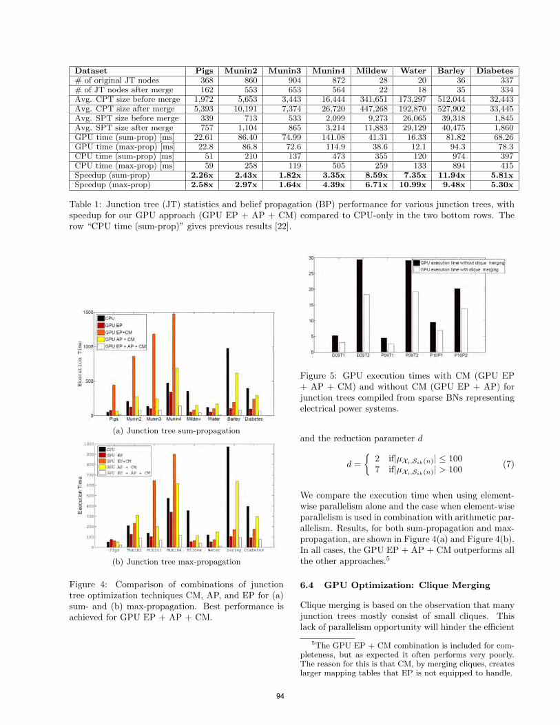
Dataset Pigs Munin2 Munin3 Munin4 Mildew Water Barley Diabetes# of original JT nodes 368 860 904 872 28 20 36 337# of JT nodes after merge 162 553 653 564 22 18 35 334Avg. CPT size before merge 1,972 5,653 3,443 16,444 341,651 173,297 512,044 32,443Avg. CPT size after merge 5,393 10,191 7,374 26,720 447,268 192,870 527,902 33,445Avg. SPT size before merge 339 713 533 2,099 9,273 26,065 39,318 1,845Avg. SPT size after merge 757 1,104 865 3,214 11,883 29,129 40,475 1,860GPU time (sum-prop) [ms] 22.61 86.40 74.99 141.08 41.31 16.33 81.82 68.26GPU time (max-prop) [ms] 22.8 86.8 72.6 114.9 38.6 12.1 94.3 78.3CPU time (sum-prop) [ms] 51 210 137 473 355 120 974 397CPU time (max-prop) [ms] 59 258 119 505 259 133 894 415Speedup (sum-prop) 2.26x 2.43x 1.82x 3.35x 8.59x 7.35x 11.94x 5.81xSpeedup (max-prop) 2.58x 2.97x 1.64x 4.39x 6.71x 10.99x 9.48x 5.30x

Table 1: Junction tree (JT) statistics and belief propagation (BP) performance for various junction trees, withspeedup for our GPU approach (GPU EP + AP + CM) compared to CPU-only in the two bottom rows. Therow “CPU time (sum-prop)” gives previous results [22].

(a) Junction tree sum-propagation

(b) Junction tree max-propagation

Figure 4: Comparison of combinations of junctiontree optimization techniques CM, AP, and EP for (a)sum- and (b) max-propagation. Best performance isachieved for GPU EP + AP + CM.

Figure 5: GPU execution times with CM (GPU EP+ AP + CM) and without CM (GPU EP + AP) forjunction trees compiled from sparse BNs representingelectrical power systems.

and the reduction parameter d

d =

2 if|µXi,Sik(n)| ≤ 1007 if|µXi,Sik(n)| > 100

(7)

We compare the execution time when using element-wise parallelism alone and the case when element-wiseparallelism is used in combination with arithmetic par-allelism. Results, for both sum-propagation and max-propagation, are shown in Figure 4(a) and Figure 4(b).In all cases, the GPU EP + AP + CM outperforms allthe other approaches.5

6.4 GPU Optimization: Clique Merging

Clique merging is based on the observation that manyjunction trees mostly consist of small cliques. Thislack of parallelism opportunity will hinder the efficient

5The GPU EP + CM combination is included for com-pleteness, but as expected it often performs very poorly.The reason for this is that CM, by merging cliques, createslarger mapping tables that EP is not equipped to handle.

94

use of the available computing resources, since a singlemessage passing will not be able to occupy the GPU.Merging neighboring small cliques, found in the S-S-Spattern, can help to increase the average size of sep-arators and cliques. Clique merging also reduces thetotal number of nodes in the junction tree, which inturn reduces the invocation overhead.

We use two parameters to determine which cliquesshould be merged–one is τs, the threshold for separa-tors’ potential table size and the other is τµ, the thresh-old for the size of the index mapping table. These pa-rameters are set manually in this paper, however ina companion paper [21] this parameter optimizationprocess is automated by means of machine learning.

In the experiments, we used both arithmetic paral-lelism and element-wise parallelism. This experimentpresents how much extra speedup can be obtained byusing clique merging and arithmetic parallelism. Theexperimental results can be found in Table 1, in therows showing the GPU execution times for both sum-propagation and max-propagation. In junction treesPigs, Munin2, Munin3 and Munin4, a considerablefraction of cliques (and consequently, separators) aresmall, in other words the S-S-S pattern is common.By merging cliques, we can significantly increase theaverage separators’ and cliques’ potential size and thusprovide more parallelism.

Comparing GPU EP + AP with GPU EP + AP +CM, the speedup for these junction trees ranged from10% to 36% when clique merging is used. However,in junction trees Mildew, Water, Barley and Diabetes,clique merging does not help much since they mainlyconsist of large cliques to start with.

Another set of experiments were performed with junc-tion trees that represent an electrical power systemADAPT [16–18]. These junction trees contain manysmall cliques, due to their underlying BNs being rel-atively sparsely connected.6 The experimental resultsare shown in Figure 5. Using clique merging, the GPUexecution times are shortened by 30%-50% for theseBNs compared to not using clique merging.

6.5 Performance Comparison: CPU

As a baseline, we implemented a sequential programon an Intel Core 2 Quad CPU with 8MB cache anda 2.5GHz clock. The execution time of the programis comparable to that of GeNie/SMILE, a widely usedC++ software package for BN inference.7 We do notdirectly use GeNie/SMILE as the baseline here, be-cause we do not know the implementation details of

6http://works.bepress.com/ole_mengshoel/7http://genie.sis.pitt.edu/

GeNie/SMILE.

In Table 1, the bottom six rows give the executiontime comparison for our CPU/GPU hybrid versus atraditional CPU implementation. The CPU/GPU hy-brid uses arithmetic parallelism, element-wise paral-lelism and clique merging. The obtained speedup forsum-propagation ranges from 1.82x to 11.94x, with anarithmetic average of 5.44x and a geometric average of4.42.

The speedup for max-propagation is similar to, but dif-ferent from sum-propagation in non-trivial ways. Theperformance is an overall effect of many factors suchas parallelism, memory latency, kernel invocation over-head, etc. Those factors, in turn, are closely correlatedwith the underlying structures of the junction trees.The speedup for max-propagation ranges from 1.64xto 10.99x, with an arithmetic average of 5.51x and ageometric average of 4.61x.

6.6 Performance Comparison: Previous GPU

We now compare the GPU EP + AP + CM tech-nique introduced in this paper with our previous GPUEP approach [22]. From results in Table 1, comparedwith the GPU EP approach [22], the arithmetic av-erage cross platform speedup increases from 3.38x (or338%) to 5.44x (or 544%) for sum-propagation. Formax-propagation8 the speedup increases from 3.22x(or 322%) to 5.51x (or 551%).

7 CONCLUSION AND FUTUREWORK

In this paper, we identified small separators as bottle-necks for parallel computing in junction trees and de-veloped a novel two-dimensional parallel approach forbelief propagation over junction trees. We enhancedthese two dimensions of parallelism by careful cliquemerging in order to make better use of the parallelcomputing resources of a given platform.

In experiments with a CUDA implementation on anNVIDIA GeForce GTX460 GPU, we explored how theperformance of our approach varies with different junc-tion trees from applications and how clique mergingcan improve the performance for junction trees thatcontains many small cliques. For sum-propagation, theaverage speedup is 5.44x and the maximum speedupis 11.94x. The average speedup for max-propagationis 5.51x while the maximum speedup is 10.99x.

In the future, we would like to see research on parame-ter optimization for both clique merging and message

8We implemented max-propagation based on the ap-proach developed previously [22].

95

passing. It would be useful to automatically changethe merging parameters for different junction treesbased on the size distribution of the cliques and sep-arators. In addition, we also want to automaticallychange the kernel running parameters for each singlemessage passing according to the size of a message. Infact, we have already made progress along these lines,taking a machine learning approach [21].

Acknowledgments

This material is based, in part, upon work supportedby NSF awards CCF0937044 and ECCS0931978.

References

[1] R. Bekkerman, M. Bilenko, and J. Langford, edi-tors. Scaling up Machine Learning: Parallel andDistributed Approaches. Cambridge University Press,2011.

[2] A. P. Dawid. Applications of a general propagationalgorithm for probabilistic expert systems. Statisticsand Computing, 2:25–36, 1992.

[3] J. Gonzalez, Y. Low, C. Guestrin, and D. O’Hallaron.Distributed parallel inference on large factor graphs.In Proc. of the 25th Conference in Uncertainty in Ar-tificial Intelligence (UAI-09), 2009.

[4] C. Huang and A. Darwiche. Inference in belief net-works: A procedural guide. International Journal ofApproximate Reasoning, (3):225–263, 1994.

[5] F. V. Jensen, S. L. Lauritzen, and K. G. Olesen.Bayesian updating in causal probabilistic network bylocal computations. Computational Statistics, pages269–282, 1990.

[6] H. Jeon, Y. Xia, and V. K. Prasanna. Parallel exactinference on a CPU-GPGPU heterogenous system. InProc. of the 39th International Conference on ParallelProcessing, pages 61–70, 2010.

[7] K. Kask, R. Dechter, and A. Gelfand. BEEM: bucketelimination with external memory. In Proc. of the26th Annual Conference on Uncertainty in ArtificialIntelligence (UAI-10), pages 268–276, 2010.

[8] D. Koller and N. Friedman, editors. Probablisticgraphic model: principle and techniques. The MITPress, 2009.

[9] A. V. Kozlov and J. P. Singh. A parallel Lauritzen-Spiegelhalter algorithm for probabilistic inference. InProc. of the 1994 ACM/IEEE conference on Super-computing, pages 320–329, 1994.

[10] S. L. Lauritzen and D. J. Spiegelhalter. Local compu-tations with probabilities on graphical structures andtheir application to expert systems. Journal of theRoyal Statistical Society, 50(2):157–224, 1988.

[11] M. D. Linderman, R. Bruggner, V. Athalye, T. H.Meng, N. B. Asadi, and G. P. Nolan. High-throughput

Bayesian network learning using heterogeneous multi-core computers. In Proc. of the 24th ACM Interna-tional Conference on Supercomputing, pages 95–104,2010.

[12] Y. Low, J. Gonzalez, A. Kyrola, D. Bickson,C. Guestrin, and J. Hellerstein. GraphLab: A newframework for parallel machine learning. In Proc. ofthe 26th Annual Conference on Uncertainty in Artifi-cial Intelligence (UAI-10), pages 340–349, 2010.

[13] O. J. Mengshoel. Understanding the scalability ofBayesian network inference using clique tree growthcurves. Artificial Intelligence, 174:984–1006, 2010.

[14] V. K. Namasivayam and V. K. Prasanna. Scalableparallel implementation of exact inference in Bayesiannetworks. In Proc. of the 12th International Confer-ence on Parallel and Distributed System, pages 143–150, 2006.

[15] D. Nilsson. An efficient algorithm for finding the mmost probable configurations in probablistic expertsystem. Statistics and Computing, pages 159–173,1998.

[16] B. W. Ricks and O. J. Mengshoel. The diagnostic chal-lenge competition: Probabilistic techniques for faultdiagnosis in electrical power systems. In Proc. of the20th International Workshop on Principles of Diag-nosis (DX-09), pages 415–422, Stockholm, Sweden,2009.

[17] B. W. Ricks and O. J. Mengshoel. Methods for prob-abilistic fault diagnosis: An electrical power systemcase study. In Proc. of Annual Conference of the PHMSociety, 2009 (PHM-09), San Diego, CA, 2009.

[18] B. W. Ricks and O. J. Mengshoel. Diagnosing in-termittent and persistent faults using static bayesiannetworks. In Proc. of the 21st International Work-shop on Principles of Diagnosis (DX-10), Portland,OR, 2010.

[19] M. Silberstein, A. Schuster, D. Geiger, A. Patney, andJ. D. Owens. Efficient computation of sum-productson GPUs through software-managed cache. In Proc.of the 22nd ACM International Conference on Super-computing, pages 309–318, 2008.

[20] Y. Xia and V. K. Prasanna. Node level primitives forparallel exact inference. In Proc. of the 19th Inter-national Symposium on Computer Architechture andHigh Performance Computing, pages 221–228, 2007.

[21] L. Zheng and O. J. Mengshoel. Optimizing parallelbelief propagation in junction trees using regression.In Proc. of 19th ACM SIGKDD Conference on Knowl-edge Discovery and Data Mining (KDD-13), Chicago,IL, August 2013.

[22] L. Zheng, O. J. Mengshoel, and J. Chong. Belief prop-agation by message passing in junction trees: Com-puting each message faster using GPU paralleliza-tion. In Proc. of the 27th Conference in Uncertaintyin Artificial Intelligence (UAI-11), pages 822–830,Barcelona, Spain, 2011.

96

Author Index

A

Agosta, John 50Almond, Russell 1B

Babagholami-Mohamadabadi, Behnam 11C

Chee, Yung En 77Chung, Gregory K.W.K. 20F

Fenton, Norman 49G

Griss, Martin 67H

Hanson, Robin 39J

Jourabloo, Amin 11K

Kerr, Deirdre 20Kim, Yoon Jeon 1L

Laskey, Kathryn 29, 39M

Manzuri-Shalmani, Mohammad. T 11Marsh, William 49Mengshoel, Ole 67, 87Moore, David A. 58N

Nicholson, Ann 77P

Perkins, Zane 49Pillai, Preeti 50Q

97

Quintana-Ascencio, Pedro 77R

Russell, Stuart 58Rafatirad, Setareh 29S

Shute, Valerie 1Sun, Feng-Tso 67Sun, Wei 39T

Tai, Nigel 49Twardy, Charles 39V

Ventura, Matthew 1W

Wilkinson, Lauchlin A.T. 77Y

Yeh, Yi-Ting 67Yet, Barbaros 49Z

Zheng, Lu 87Zolfaghari, Mohammadreza 11

98