Proceedings of the 13th InternationalWorkshop on Logic Programming

Environments

Fred MesnardAlexander Serebrenik (Eds.)

Report CW371, November 2003

Katholieke Universiteit LeuvenDepartment of Computer ScienceCelestijnenlaan 200A – B-3001 Heverlee (Belgium)

Proceedings of the 13th InternationalWorkshop on Logic Programming

Environments

Fred MesnardAlexander Serebrenik (Eds.)

Report CW371, November 2003

Department of Computer Science, K.U.Leuven

Preface

This volume contains papers presented at WLPE 2003, the 13th Interna-tional Workshop on Logic Programming Environments. The aim of WLPE is toprovide an informal meeting for researchers working on tools for developmentand analysis of logic programming. This year, the emphasis is on the presenta-tion, pragmatics and experiences of such tools.

WLPE 2003 takes place in Tata Institute of Fundamental Research, Mum-bai, India on December 8 and is a part of a bigger event, ICLP 2003, the 19thInternational Conference on Logic Programming, holding in conjunction withASIAN 2003, the Eighth Asian Computing Science Conference, and FSTTCS2003, the 23rd Conference on Foundations of Software Technology and Theor-etical Computer Science. This workshop continues the series of successful in-ternational workshops on logic programming environments held in Ohio, USA(1989), Eilat, Israel (1990), Paris, France (1991), Washington, USA (1992),Vancouver, Canada (1993), Santa Margherita Ligure, Italy (1994), Portland,USA (1995), Leuven, Belgium and Port Jefferson, USA (1997), Las Cruces,USA (1999), Paphos, Cyprus (2001) and Copenhagen, Denmark (2002).

We would like to express our gratitude to the ICLP organisers for hosting theworkshop. Special thanks go to R.K.Shyamasundar for taking care of the manyorganisational matters, in particular, printing these proceedings. Also we wouldlike to thank the program committee members for reviewing and discussing thesubmissions as well as the authors for submitting their work.

Out of 9 submissions the program committee has selected 5 works for present-ation. In addition, Jan Wielemaker (University of Amsterdam, The Netherlands)was invited to present a number of typical problems Prolog users are faced withand illustrate how tools developed in SWI-Prolog may help to find them.

Fred MesnardAlexander SerebrenikMumbai, December 2003

Organisation

13th Workshop on Logic Programming EnvironmentsWLPE 2003 December 8, 2003, Mumbai, India

Workshop organisers:

Fred Mesnard (Universite de La Reunion, France)Alexander Serebrenik (coordinator, Katholieke Universiteit Leuven, Bel-gium)

Program committee:

Roberto Bagnara (Universita degli studi di Parma, Italy)Manuel Carro (Universidad Politecnica de Madrid, Spain)Mireille Ducasse (INSA/IRISA, Rennes, France)Pat Hill (University of Leeds, U.K.)Naomi Lindenstrauss (Hebrew University of Jerusalem, Israel)Jan-Georg Smaus (Universitat Freiburg, Germany)Fausto Spoto (Universita di Verona, Italy)Alexandre Tessier (Universite d’Orleans, France)

Reviewers:

Pieter BekaertMaurice BruynoogheDaniel CabezaPierre DeransartGerard FerrandJose Manuel GomezArnaud LallouetTom SchrijversZoltan SomogyiJoost Vennekens

Table of Contents

An Overview of the SWI-Prolog Programming Environment . . . . . . . . . . . 1Jan Wielemaker

TCLP: A type checker for CLP(X) . . . . . . . . . . . . . . . . . . . . . . . . . . . . . . . . 17Emmanuel Coquery

Analyzing and Visualising Prolog programs based on XML representations 31Dietmar Seipel, Marbod Hopfner, Bernd Heumesser

Demonstration proposal: Debugging constraint problems with portable tools 46Pierre Deransart, Ludovic Langevine and Mireille Ducasse

Proving Termination One Loop at a Time . . . . . . . . . . . . . . . . . . . . . . . . . . 48Michael Codish and Samir Genaim

Hasta-La-Vista: Termination Analyser for Logic Programs . . . . . . . . . . . . . 60Alexander Serebrenik and Danny De Schreye

Constructive combination of crisp and fuzzy logic in a Prolog compiler . . 75Susana Munoz, Claudio Vaucheret and Sergio Guadarrama

An Overview of the SWI-Prolog ProgrammingEnvironment

Jan Wielemaker

Social Science Informatics (SWI),University of Amsterdam,

Roetersstraat 15, 1018 WB Amsterdam, The Netherlands,jan@swi.psy.uva.nl

Abstract. The Prolog programmer’s needs have always been the focusfor guiding the development of the SWI-Prolog system. This article ac-companies an invited talk about how the SWI-Prolog environment helpsthe Prolog programmer solve common problems. It describes the centralparts of the graphical development environment as well as the commandline tools which we see as vital to the success of the system. We hopethis comprehensive overview of particularly useful features will both in-spire other Prolog developers, and help SWI-Prolog users to make moreproductive use of the system.

1 Introduction

SWI-Prolog has become a popular Free Software implementation of theProlog language. Distributed freely through the internet, it is di!cult toget a clear picture about its users, how these users use the system andwhich aspects of the system have contributed most to its popularity. Partof the users claim the programmer’s environment described in this articleis an important factor.

The majority of the SWI-Prolog users are students using it for their as-signments. The community of developers, however, expend e"ort on largeportable Prolog applications where scalability, (user-) interfaces, network-ing are often important characteristics. Compared to the students, whoare mostly short-term novice users, we find many expert software de-velopers in the research and development community.

The material described in this paper is the result of about 18 yearsexperience as a Prolog programmer and developer of the SWI-Prologsystem. Many of the described tools are features not unique to SWI-Prologand can be found in other Prolog implementations or other programminglanguage environments. Experiments are yet to be performed to evaluatethe usefulness of features and therefore the opinions presented are strictlybased on our own experiences, observations of users, and E-mail reactions.

After describing the SWI-Prolog user community in Sect. 2 we de-scribe some problems Prolog programmers frequently encounter in Sect. 3.In Sect. 4 we describe the command line tools, and in Sect. 5 the graphicaltools written in SWI-Prolog’s XPCE GUI toolkit [10].

2 User profiles

Students having to complete assignments for a Prolog course have verydi"erent needs from professionals developing large systems. They wanteasy access to common tasks as closely as possible to the conventionsthey are used to. Scalability of supporting tools is not an importantissue as the programs do not require many resources. Visualization ofterms and program state can concentrate their contribution to explan-ation and disregard, for example, the issue that most graphical repres-entations scale poorly. The SWI-Prolog-Editor1 shell for MS-Windows byGerhard Rohner makes SWI-Prolog much more natural to a student whois first of all familar with MS-Windows.

SWI-Prolog comes from the Unix and Emacs tradition and targets theprofessional programmer who uses it frequently to develop large Prolog-based applications. As many users in this category have their existinghabits, and a preferred set of tools to support these, SWI-Prolog avoidspresenting a single comprehensive IDE (Integrated Development Environ-ment), but instead provides individual components that can be combinedand customised at will.

3 Problems

Many problems that apply to programming in Prolog also relate the pro-gramming in other languages. Some, however, are Prolog specific. Prologenvironments can normally be used interactively and changed dynamic-ally.

3.1 Problem areas

– Managing sourcesBesides the normal problems such as locating functions and files, Pro-log requires a tool that manages consistency between the sources andrunning executable during the interactive test-edit cycle. Section 4.1and Sect. 5.1 describe the SWI-Prolog support to manage sources.

1 http://www.bildung.hessen.de/abereich/inform/skii/material/swing/indexe.htm

– Entering and reusing queriesInteraction through the Prolog top level is vital for managing the pro-gram and testing individual predicates. Command line editing, com-mand completion, do what I mean (DWIM) correction, history, andstoring the values of top level variables reduces typing and speed upthe development cycle.

– Program completeness and consistencySWI-Prolog has no tradition in rigid static analysis. It does provide aquick completeness test as described in Sect. 4.6 which runs automat-ically during the test-edit cycle. A cross-referencer is integrated intothe built-in editor (Sect. 5.1) and provides immediate feedback to theprogrammer about common mistakes while editing a program.

– Error contextIf an error occurs, it is extremely important to provide as much contextas possible. The SWI-Prolog exception handling di"ers slightly fromthe ISO standard to improve such support. See Sect. 4.10.

– Failure/wrong answerA very common and time consuming problem are programs producingthe wrong (unexpected) answer without producing an error. Althoughresearch has been carried out to attribute failure and wrong answersto specific procedures [3, 9], none of this is realised in SWI-Prolog.

– DeterminismAlthough experience and discipline help, controlling determinism inProlog programs to get all intended solutions quickly is a very commonproblem. The source-level debugger (Sect. 5.3) displays choicepointsand provides immediate graphical feedback on the e"ects of the cut,greatly simplifying this task and improving understanding for novices.

– Performance bottlenecksBeing a high level language, the relation between Prolog code andrequired resources to execute it is not trivial. Profiling tools cannot fixpoor overall design, but do provide invaluable insight to programmer.See Sect. 5.4.

– Porting programs from other systemsPorting Prolog programs has been simplified since more Prolog sys-tems have adopted part I of the ISO standard. Di"erent extensionsand libraries cause many of the remaining problems. Compiler warn-ings and static analysis form the most important tools to locate theproblem areas quickly. A good debugger providing context on errorstogether with support for the test-edit cycle improve productivity.

4 Command line Tools

4.1 Supporting the edit cycle

Prolog systems o"er the possibility to interactively edit and reload a pro-gram even while the program is running. There are two simple but veryfrequent tasks involved in the edit-reload cycle: finding the proper source,and reloading the modified source files. SWI-Prolog supports these taskswith two predicates:

makeSWI-Prolog maintains a database of all loaded files with the filelast-modified time stamp when it was loaded and —for the sake ofmodules— the context module(s) from which the file was loaded. Themake/0 predicate checks whether the modification time of any of theloaded files has changed and reload these file into the proper modulecontext. This predicate has proven to be very useful.

edit(+Specifier)Find all entities with the given specifier. If there are multiple entitiesrelated to di"erent source-files ask the user for the desired one andcall the user-defined editor on the given location. All entities implies(loaded) files, predicates and modules. Both locating named entitiesand what is required to call the editor on a specific file and line canbe hooked to accomodate extensions (e.g. XPCE classes) and di"er-ent editors. Furthermore, SWI-Prolog maintains file and line-numberinformation for modules and clauses. Below is an example:

?- edit(rdf_tree).Please select item to edit:

1 class(rdf_tree) ’rdf_tree.pl’:272 module(rdf_tree) ’rules.pl’:460

Your choice? 2

SWI-Prolog’s completion and DWIM described in Sect. 4.4 andSect. 4.3 improve the usefulness of these primitives.

4.2 Autoloading and auto import

Programmers tend to be better at remembering the names of library pre-dicates than the exact library they belong to. Similar, programmers of

large modular applications often have a set of personal favourites andapplication specific goodies. SWI-Prolog supports this style of program-ming with two mechanisms, both of which require a module system. TheSWI-Prolog module system is very close to the Quintus and SICStus Pro-log module systems [2].

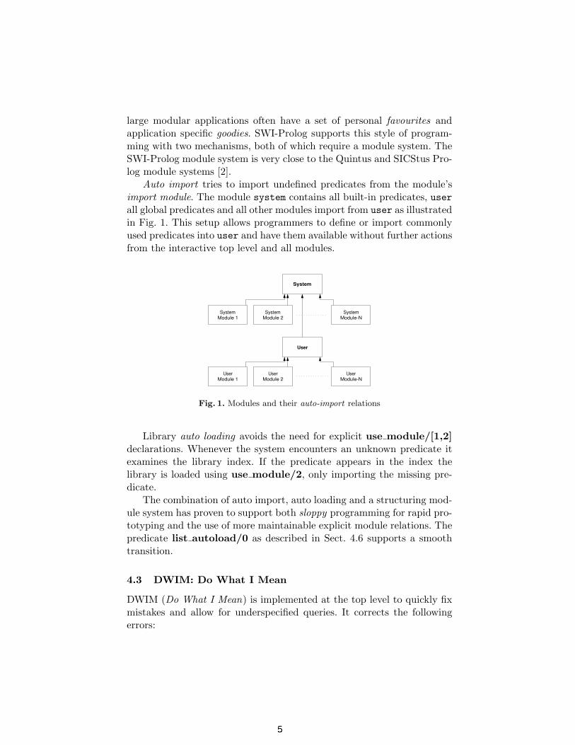
Auto import tries to import undefined predicates from the module’simport module. The module system contains all built-in predicates, userall global predicates and all other modules import from user as illustratedin Fig. 1. This setup allows programmers to define or import commonlyused predicates into user and have them available without further actionsfrom the interactive top level and all modules.

System

User

SystemModule 1

SystemModule 2

SystemModule-N

UserModule 1

UserModule 2

UserModule-N

Fig. 1. Modules and their auto-import relations

Library auto loading avoids the need for explicit use module/[1,2]declarations. Whenever the system encounters an unknown predicate itexamines the library index. If the predicate appears in the index thelibrary is loaded using use module/2, only importing the missing pre-dicate.

The combination of auto import, auto loading and a structuring mod-ule system has proven to support both sloppy programming for rapid pro-totyping and the use of more maintainable explicit module relations. Thepredicate list autoload/0 as described in Sect. 4.6 supports a smoothtransition.

4.3 DWIM: Do What I Mean

DWIM (Do What I Mean) is implemented at the top level to quickly fixmistakes and allow for underspecified queries. It corrects the followingerrors:

– Simple spelling errorsDWIM checks for missing, extra and transposed characters that resultfrom typing errors.

– Word breaks and orderDWIM checks for multi-word identifiers using di"erent conventions(e.g. fileExists vs. file exists) as well as di"erent order (e.g. exists filevs. file exists)

– Arity mismatchOf course such errors cannot be corrected.

– Wrong moduleDWIM adds a module specification to predicate references that lackone or replaces a wrong module specification.

DWIM is used in three areas. Queries typed at the top level arechecked and if there is a unique correction the system prompts whetherto execute the corrected rather than the typed query. Especially addingthe module specifier improves interaction from the top level when usingmodules. If there is no unique correction the system reports the missingpredicates and all close candidates. Queries of the development systemsuch as edit/1 and spy/1 provide alternative matches one-by-one. Spy/1and trace/1 act on the specified predicate in any module if the moduleis omitted. Finally, if a predicate existence error reaches the top level theDWIM system is activated to report likely candidates.

4.4 Command line editing

Developers spend a lot of time entering commands for the developmentsystem and (test-)queries for (parts of) their application under develop-ment. SWI-Prolog provides the following features to support this:

– Using (GNU-)readlineEmacs-style editing is supported in the Unix version based on theGNU readline library and in Windows using our own code. This facil-itates quick and natural command reuse and editing. In addition, com-pletion is extended with completion on alphanumerical atoms whichallow for fast typing of long predicate identifiers and atom argumentsas well as inspect the possible alternative (using Alt-?). The comple-tion algorithm uses the builtin completion of files if no atom matches,which ensures that quoted atoms representing a file path is completedas expected.

– Command line historySWI-Prolog provides a history facility that resembles the Unix cshand bash shells. Especially viewing the list of executed commands isa valuable feature.

– Top level bindingsWhen working at the Prolog top level, bindings returned by previousqueries are normally lost while they are often required for furtheranalysis of the current Prolog state or to test further queries. Forthis reason SWI-Prolog stores the resulting bindings from top levelqueries, provided they are not too large (default ! 1000 tokens) inthe database under the name of the used variable. Top level queryexpansion replaces terms of the form $Var ($ is a prefix operator)into the last recorded binding for this variable. New bindings do tobacktracking or new queries overwrite the old value.This feature is particularly useful to query the state of data stored inrelated dynamic predicates and deal with handles provided by externalstores. Here is a typical example using XPCE that avoids typing orcopy/paste of the object reference.

?- new(X, picture).

X = @12946012?- send($X, open).

4.5 Compiler

An important aspect of the SWI-Prolog compiler is its performance. Load-ing the 21 Mb sources of WordNet [7] requires 6.6 seconds from the sourceand 1.4 seconds from precompiled virtual machine code (Multi-threadedSWI-Prolog 5.2.9, SuSE Linux on dual AMD 1600+ using one thread).Fast compilation is very important during the interactive development oflarge applications.

SWI-Prolog supports the commonly found set of compiler warnings:syntax errors, singleton variables, predicate redefinition, system predicateredefinition and discontiguous predicates. Messages are processed by thehookable print message/2 predicate and where possible associated witha file and line number. The graphics system contains a tool that exploitsthe message hooks to create a window with error messages and warningsthat can be selected to open the associated source location.

4.6 Quick consistency check

The library check provides quick tests on the completeness of the loadedprogram. The predicate list undefined/0 searches the internal databasefor predicate structures that are undefined (i.e. have no clauses and arenot defined as dynamic or multifile). Such structures are created by thecompiler for a call to a predicate that is not yet defined. In addition thesystem provides a primitive that returns the predicates referenced from aclause by examining the compiled code. Figure 2 provides partial outputrunning list undefined/0 on the chat 80 [8] program:

1 ?- [library(chat)].% ...% library(’chat/chat’) compiled into chat 0.18 sec, 493,688 bytes% library(chat) compiled into chat 0.18 sec, 494,756 bytes

Yes2 ?- list_undefined.% Scanning references for 9 possibly undefined predicatesWarning: The predicates below are not defined. If these are definedWarning: at runtime using assert/1, use :- dynamic Name/Arity.Warning:Warning: chat:ditrans/12, which is referenced byWarning: 5-th clause of chat:verb_kind/6

Fig. 2. Using list undefined/0 on chat 80 wrapped into the module chat. To savespace only the first of the 9 reported warnings is included. The processing requires0.25 sec. on a 733 Mhz PIII.

The list autoload/0 predicate lists undefined predicates that can beautoloaded from one of the libraries. It is illustrated in Fig. 3.

3 ?- list_autoload.% Into module chat (library(’chat.pl’))% display/1 from library(edinburgh)% last/2 from library(lists)% time/1 from library(statistics)% Into module user% prolog_ide/1 from library(swi_ide)

Fig. 3. Using list autoload/0 on chat 80

4.7 Help and explain facility

The help facility uses outdated but still e"ective technology. The LATEXmaintained source is translated to plain text. A generated Prolog indexfile provides character ranges for predicate descriptions and sections inthe manual. Each predicate has, besides the full documentation, a ±40 character summary description used for apropos search as well as toprovide a summary string in the editor as illustrated in Fig. 4.

The explain facility examines the database to gather all informationknown about an identifier (atom). Information displayed includes predic-ates with that name and references to the atoms, compound terms andpredicates with the given name. Here is an example:

explain(setof)."setof" is an atom

Referenced from 1-th clause of chat:decomp/3system:setof/3 is a built-in meta predicate imported from module

$bags defined in/staff/jan/lib/pl-5.2.9/boot/bags.pl:59Summary: ‘‘Find all unique solutions to a goal’’Referenced from 6-th clause of chat:satisfy/1Referenced from 7-th clause of chat:satisfy/1Referenced from 1-th clause of chat:seto/3

The graphical front end is described in Sect. 5.5.

4.8 File commands

Almost too trivial to name, but the predicates ls/0, cd/1 and pwd/0are used very frequently.

4.9 Debugging from the terminal

SWI-Prolog comes with two tracers, a traditional 4-port debugger [1] tobe used from the terminal and a graphical source level debugger which isdescribed in Sect. 5.3. Less frequently seen features of the trace are:

– Single keystroke operationIf the terminal supports it, commands are entered without waiting forreturn.

– List choicepointsThe tracer can provide a list of active choicepoints, similar to the goalstack, to facilitate choicepoint tuning and debugging.

– The ‘up’ commandThe ‘up’ command is like the traditional ‘skip’ command, but skipsto the exit or failure of the parent goal rather than the current goal.It is very useful to stop tracing the details of failure driven controlstructures.

– SearchThe system can search for a specific port and goal that unifies withan entered term. The command /f foo(_, bar) will go into inter-active debugging if foo/2 where the second argument unifies with barreaches the fail (f) port.

In addition to interactive debugging two types of non-interactive de-bugging are provided. Using trace(Predicate, Ports), the system printsall passes to the indicated ports of Predicate.

The library debug is a lightweight infrastructure to handle printingdebugging messages (logging) and assertions. The library exploits goal-expansion to avoid runtime overhead when compiled with optimisationturned on. Debug messages are associated to a Topic, an arbitrary Pro-log term used to group debug messages. Normally the Topic is an atomdenoting some function or module of the application. Using Prolog uni-fication of the active topics and the topic registered with the messageprovides opportunity for creativity.

debug(+Topic, +Format, +Arguments)Prints a message through the system’s print message/2 messagedispatching mechanism if debugging is enabled on Topic.

debug/nodebug(+Topic)Enable/disable messages for which Topic unifies. Note that topics arearbitrary Prolog terms, so debug( ) enables all debugging messages.

list debug topicsList all registered topics and their current enable/disable setting. Allknown topics are collected during compilation using goal-expansion.

assume(:Goal)Assume that Goal can be proven. Trap the debugger if Goal fails.This facility is derived from the C-language assert() macro definedin <assert.h>, renamed for obvious reasons. More formal assertionlanguages are described in [6, 5].

4.10 Exception context

On exception handling, the ISO standard dictates ‘undo’ back to the stateat entry of a catch/3 before unifying the ball with the catcher. SWI-

Prolog however uses a di"erent technique. It walks the stack searchingfor a matching catcher without undoing changes. If it finds a matchingcatch/3 call or when reaching a call from foreign code that indicatesit is prepared to handle exceptions it performs the required ‘undo’ andexecutes the handler. The advantage is that if there is no handler forthe exception the entire program state is still intact. The debugger isstarted immediately and can be used to examine the full context of theexception.2

5 Graphical Tools

5.1 Editor

PceEmacs is an Emacs clone written in XPCE/Prolog. It has two featuresthat make it of special interest. It can be programmed in Prolog and there-fore has transparent access to the environment of the application beingdeveloped, and the editor’s bu"er can be opened as a Prolog I/O stream.Based on these features, the level of support for Prolog development isfar beyond what can be achieved in a stand-alone editor. Whenever theuser pauses for two seconds the system performs a full cross-reference ofthe editing bu"er, categorising and colouring predicates, goals and gen-eral Prolog terms. Predicates are categorised as exported, called and notcalled. Goals are categorised as builtin, imported, auto-imported, locallydefined, dynamic, (direct-)recursive and undefined. Goals have a menuthat allows jumps to the source, documentation (builtin), and listing ofclauses (dynamic). Singleton variables are highlighted. If the cursor ap-pears inside a variable all other occurrences of this variable in the clauseare underlined. Figure 4 shows a typical screenshot.

5.2 Prolog Navigator

The Prolog Navigator provides a hierarchical overview of a project direct-ory and its Prolog files. Prolog files are categorised as one of loaded or notloaded and are expanded to the predicates defined in them. The definedpredicates are categorised as one of exported, normal, fact and unrefer-enced. Expanding predicates expands the call tree. The Navigator menusprovide loading and editing files and predicates as well as the setting oftrace- and spy-points. See Fig. 5.2 These issues have been discussed on the comp.lang.prolog newsgroup, April 15-18

2002, subject “ISO catch/throw question”.

Fig. 4. PceEmacs in action

Fig. 5. The Prolog Navigator

5.3 Source-level Debugger

The SWI-Prolog debugger calls a hook (prolog trace interception/4) be-fore reverting to the built-in command line debugger. The built in pro-log frame attribute/3 provides the infrastructure to analyse the Pro-log stacks, providing information on the goal-stack, variable bindings andchoicepoints. These hooks are used to realise more advanced debuggerssuch as the source-level debugger described in this section. The source-level debugger provides three views (Fig. 6):

– The sourceAn embedded PceEmacs (see Sect. 5.1) running in read-only modeshows the current location, indicating the current port using colourand icons. PceEmacs also allows the setting of breakpoints at a spe-cific call in specific clause. Breakpoints provide finer and more intu-itive control where to start the debugger than traditional spy-points.Breakpoints are realised by replacing a virtual machine instructionwith a break instruction which traps the debugger, finds the instruc-tion it replaces in a table and executes this instruction.

– VariablesThe debugger displays a list of variables appearing in the currentframe with their name and current binding in the top-left window. Therepresentation of values can be changed using the familiar portray/1hook. Double-clicking a variable-value opens a separate window show-ing the variable binding. This window uses indentation to make thestructure of the term more explicit and has a menu to control thelayout.

– The stackThe top-right window shows the stack as well as the recent activechoicepoints. Any node can be selected to examine the context of thatnode. The stack view allows one to quickly examine choicepoints leftafter a goal succeeded. Besides showing the location of the choicepointitself, the ‘up’ command can be used to examine the parent framecontext of a choicepoint.

5.4 Execution Profiler

The Execution Profiler builds a call-tree at runtime and ticks the numberof calls and redos to each node in this call-tree. The time spent in each

Fig. 6. The Source-level Debugger

node is established using stochastic sampling.3 Recording the call-tree iscomplicated by three factors.

– Last call optimisationDue to last call optimisation exit ports are missing from the executionmodel. This problem is solved by storing the call-tree node associatedwith a goal in the environment stack, providing the exit with a ref-erence to the node exited. Recording an exit can now exit all nodesuntil it reaches the referenced node.

– RedoHaving a reference from each environment frame to the call-tree nodealso greatly simplifies finding the proper location in the call-tree on aredo.

– RecursionTo avoid the uncontrolled expanding of the call-tree the system mustrecord recursive calls. The problem lies in the definition of recursion.The most naıve definition is that recursion happens if there is a par-ent node running the same predicate. In this view meta predicateswill often appear as unwanted ‘recursive predicates’ as will predicatescalled in a totally di"erent context. The system provides noprofile/1to indicate some predicates do not create a new node and their time isincluded with their parent node. Examples are call/1, catch/3 andcall cleanup/2. Calls are now regarded recursive if the parent node

3 Using SIGPROF on Unix and using a separate thread and a multi-media timer inMS-Windows.

runs the same predicate (direct recursion) or somewhere in the parentnodes of the call-tree we can find a node running the same predicatewith the same immediate parent.

Prolog primitives are provided to extract all information from the re-corded call-tree. A graphical Prolog profiling tool presents the informationinteractively similar to the GNU gprof [4] tool (see Fig. 7).

Fig. 7. The Profiler

5.5 Help System

The GUI front end to the help functionality described in Sect. 4.7 addshyperlinks and hierarchical context to the command line version as illus-trated in Fig. 8.

Fig. 8. Graphical front end to the help system

6 Conclusions

In this paper we have described commonly encountered tasks which Pro-log programmers spend much of their time on, which tools can help solv-

ing them as well as an overview of the programming environment toolsprovided by SWI-Prolog. Few of these tools are unique to SWI-Prologor very advanced. The popularity of the environment can possibly beexplained by being complete, open, portable, scalable and free.

Acknowledgements

XPCE/SWI-Prolog is a Free Software project which, by its nature, profitsheavily from user feedback and participation. We would like to thankSteve Moyle and Anjo Anjewierden for their comments on draft versionsof this paper.

References

1. Lawrence Byrd. Understanding the control flow of Prolog programs. In S.-A.Tarnlund, editor, Proceedings of the Logic Programming Workshop, pages 127–138,1980.

2. M. Carlsson, J. Widen, J. Andersson, S. Anderson, K. Boortz, H. Nilson, andT. Sjoland. SICStus Prolog (v3) Users’s Manual. SICS, PO Box 1263, S-164 28Kista, Sweden, 1995.

3. Mireille Ducasse. Analysis of failing Prolog executions. In Workshop on LogicProgramming Environments, pages 2–9, 1991.

4. Susan L. Graham, Peter B. Kessler, and Marshall K. McKusick. gprof: a callgraph execution profiler. In SIGPLAN Symposium on Compiler Construction,pages 120–126, 1982.

5. M. Hermenegildo, G. Puebla, and F. Bueno. Using global analysis, partial spe-cifications, and an extensible assertion language for program validation and debug-ging. In The Logic Programming Paradigm: a 25-Year Perspective, pages 161–192.Springer-Verlag, 1999.

6. Marija Kulas. Debugging Prolog using annotations. In Mireille Ducasse, AnthonyKusalik, and German Puebla, editors, Electronic Notes in Theoretical ComputerScience, volume 30. Elsevier, 2000.

7. G. Miller. WordNet: A lexical database for English. Comm. ACM, 38(11), Novem-ber 1995.

8. Fernando C. N. Pereira and Stuart M. Shieber. Prolog and Natural-LanguageAnalysis. Number 10 in CSLI Lecture Notes. Center for the Study of Languageand Information, Stanford, California, 1987. Distributed by Chicago UniversityPress.

9. E. Y. Shapiro. Algorithmic Program Debugging. MIT Press, Cambridge, MA, 1983.10. Jan Wielemaker and Anjo Anjewierden. An architecture for making object-oriented

systems available from Prolog. In Alexandre Tessier, editor, Computer Science,abstract, 2002. http://lanl.arxiv.org/abs/cs.SE/0207053.

TCLP: A type checker for CLP(X )

Emmanuel CoqueryEmmanuel.Coquery@inria.fr

November 7, 2003

Abstract

This paper is a presentation of TCLP: a prescriptive type checker forProlog/CLP(X ). Using parametric polymorphism, subtyping and overload-

ing, TCLP can be used with practical constraint logic programs that may use

meta-programming predicates, coercions between constraint domains (like FDand B) and constraint solver definitions, including the CHR language. It also

features type inference for variables and predicates, so the user can get rid ofnumerous type declarations.

1 Introduction

Traditionally, the class CLP(X ) of constraint logic programs, introducedby Ja!ar and Lassez [11], is untyped. One of the advantages of beinguntyped is programming flexibility. For example, -/2 can be used asthe classical arithmetic operator as well as a constructor for pairs. Onthe other hand, type checking allows the static detection of some pro-gramming errors, like for example calling a predicate with an illegalargument.

Several type systems have been created for (constraint) logic pro-gramming. The type system of Mycroft and O’Keefe [12, 15] is an adap-tation of the Damas-Milner type system [6] to logic programming. Ithas been implemented in Godel [10] and Mercury [19]. This type systemuses parametric polymorphism, that is, parameters (i.e. type variables)are allowed as and in types. For example the type list has an argu-ment to specify the type of elements occurring in the list. However thistype system is not flexible enough to be used with meta-programmingpredicates, such as arg/3, =../2 or assert/1.

Subtyping is a fundamental concept introduced by Cardelli [2] andMitchell [14]. The power of subtyping resides in the subtyping rule whichstates that an expression of type ! can be used instead of an expressionof type ! ! provided that ! is a subtype of ! !:

(Sub)U ! t : ! , ! " ! !

U ! t : ! !

Subtyping can be used to deal with meta-programming by the introduc-tion of a type term as a supertype of all types. For example, the subtyperelation list(") " term, allows to type check the query arg(N,[X|L],T),using the type int # term# term $ pred for arg/3, although the secondargument is a list. Subtyping can also be used for coercions betweenconstraint domains. For example, it is possible to share variables be-tween CLP(B), with type boolean , and CLP(FD), with type int , simply

1

by adding the subtyping relation boolean < int . This way B variablescan be used with FD predicates.

Most of the type systems with subtyping that where proposed forconstraint logic programs are descriptive type systems, i.e. they aim todescribe the set of terms for which a predicate is true. On the other hand,there where only few prescriptive type systems with subtyping for logicprogramming [1, 7, 13, 16, 18]. Moreover, in these systems, subtypingrelations between type constructors with di!erent arities, as in list(") <term, are not allowed. Algorithms to deal with such subtyping relations,called non-structural non-homogeneous subtyping, can be found in [17,20] in the case where the subtyping order forms a lattice, or in [4] forthe case of quasi-lattices.

The combined use of subtyping and parametric polymorphism thuso!ers a great programming flexibility. Still, it can not address the firstexample given in this paper, that is -/2 being viewed sometimes as thearithmetic operator and sometimes as a constructor of pairs (as in thepredicate keysort/2). The solution to this problem resides in overload-ing. Overloading consists in assigning multiple types to a single symbol.This notion has already been used in numerous languages, such as C,to deal with multiple kinds of numbers in arithmetic operations. Withoverloading, -/2 can have both type int expr# int expr $ int expr andtype "# # $ pair (",#).

In this paper, we describe TCLP, a type checker for Prolog/CLP(X ),written in SICStus Prolog with Constraint Handling Rules (CHR) [9].The type system of TCLP combines parametric polymorphism, subtyp-ing and overloading in order to keep the flexibility of the traditionallyuntyped CLP(X ) languages, yet statically detecting programming er-rors. Section 2 shows examples of how the type system takes advantageof these three features. Section 3 presents the type system of TCLP. Insection 4, we describe the basic type declarations and output of TCLP,while section 5 shows how the type system can be extended to han-dle constraint solver programming, like new CLP(FD) constraints orCHR rules. Some benchmarks are presented in section 6 and section 7concludes.

2 Motivating examples

The aim of the TCLP type checker is to introduce a typing discipline inconstraint logic programs in order to find programming errors, while of-fering enough flexibility for practical programming. That means dealingwith Prolog/CLP(X ) programming facilities like meta-programming orthe simultaneous use of multiple constraint solvers. This goal is achievedusing a combination of parametric polymorphism, subtyping and over-loading. In the rest of this section, we give examples of how they areused in TCLP.

2.1 Prolog examples

A first use of parametric polymorphism is the typing of structures thatmay be used with any type of data. For example, using the type list(")for lists allows typing [1,2] with the type list(int) and [’a’,’b’] withthe type list(char ). A consequence is the use of polymorphic types forpredicates manipulating these data structures in a generic way. For

example, the type of the predicate append/3 for concatenating lists islist(")# list(")# list (") $ pred . Of course, some other predicates mayuse non generic types when manipulating the data inside structures, likesum list/2 having type list(int) # int $ pred .

Another use of parametric polymorphism is for constraints or pred-icates that can be used on any term, the best example being =/2 withtype " # " $ pred . This type simply express that the two argumentsof =/2 must have the same type. Another example resides in term com-parison predicates like ’@=<’/2, which also has type "# " $ pred .

On the other hand, predicates for manipulating terms cannot betyped using only parametric polymorphism. An example is the predi-cate =../2 for decomposing terms. Indeed T=..L unifies L with the listconstituted by the head constructor of T and the arguments of T. Thismeans that L is an non-homogeneous list. Subtyping provides a solutionfor typing this predicate, through the introduction of the type term asthe supertype of all types, that is for all types ! , ! " term. Using thetype term # list(term) $ pred for =../2, it is possible to type check aquery like [1] =.. [’.’,1,[]] with type list(int) for [1], atom for’.’, int for 1, list(") for [] and list(term) for [’.’,1,[]].

Subtyping is also interesting when typing programs that use dynamicpredicates, using assert/1. The type of assert/1 is clause $ pred andthe type of ’:-’/2 is pred # goal $ clause. This allows typing querieslike assert((p(X) :- X<1)). However, without subtyping, queries likeassert(p(1)) are not correctly typed because p(1) would be typedpred , while assert/1 expects the type clause. Using subtyping withpred < clause, p(1) is seen with the type clause and the query is well-typed.

The operator -/2, as showed in the introduction, provides a goodexample of the use of overloading, with types int expr # int expr $int expr , float expr # int expr $ float expr , int expr # float expr $float expr , float expr #float expr $ float expr and "## $ pair (",#).This example shows the more classical overloading of -/2 with respectto the di!erent kinds of number as well as its use as a coding for pairs.In this case, subtyping can also be used to deal with the di!erent kindof numbers, with int expr < float expr , using the type "# " $ "," "float expr . However, in the Prolog dialects that we considered, theunification 1=1.0 fails. This led us to choose overloading instead ofsubtyping for dealing with numerical expressions, thus making a cleardistinction in types between integers and floats. An other example is=/2. It is used both as the equality constraint and to build pairs ofthe form Name=Var in an option of the predicate read term/3. Thusis has both types " # " $ pred and atom # term $ varname. Otherexamples include options shared by several di!erent predicates or ’,’/2used both as the conjunction and as a constructor for sequences.

2.2 Combining constraint domains

A first example is the combination of the Herbrand domain CLP(H) withan other domain, such as CLP(FD). Prolog is mainly used to handledata structures and for posting constraints. However there can be astronger interaction when defining, e.g., predicates for labelling. Thetype used to represent FD is int , already present in the type hierarchyof CLP(H). This way FD variables can be also used as Prolog variableswhen needed.

Another interesting example is combining CLP(FD) and CLP(B).Indeed, variables can be shared between the two constraint solvers. Thisis possible when B is represented as the set {0,1}. In this case 0 and 1have type boolean and boolean < int . In this way, B variables can alsobe used with FD constraints.

A last example is reified constraints. This represent a combinationof CLP(H), CLP(FD) and CLP(B). Constraints like ’#<=>’/2 acceptother constraints as arguments. In order to handle these cases, FDconstraints are typed with type fd constraint . The subtype relationsfd constraint < pred and fd constraint < boolean expr allows theseconstraints to be used both in boolean expressions and as predicatesin Prolog clauses.

3 The type system

3.1 CLP(X ) programs

CLP programs are built upon a denumerable set V of variables, a finiteset S of symbols, given with their arity, a set F % S of function symbolsand a set P % S of predicate and constraint symbols. P is supposed tocontain the equality constraint symbol =/2. Terms are built upon F&V .An atom is of the form p(t1, . . . , tn), where p/n ' P and t1, . . . , tn areterms. A query is a finite sequence of atoms. When it is necessary todistinguish predicate atoms (built using a predicate symbol) and con-straint atoms (built with a constraint symbol), queries are noted c | "where c is the constraint part of the query and " is the predicate partof the query. A clause is an expression A ( Q where A is a predicateatom and Q is a query. A constraint logic program is a set of clausesand queries.

The execution model we consider for constraint logic programs is theCSLD rewriting relation :Definition 1 Let P be a CLP(X ) program. The rewriting relation)$CSLD over queries is defined as the smallest relation satisfying thefollowing CSLD rule:

p(N1, . . . , Nk) ( c! | A1, . . . , An ' $(P )X |= *(c + M1 = N1 + . . . + Mk = Nk + c!)

c | ", p(M1, . . . , Mk),"! )$CSLD

c, M1 = N1, . . . , Mk = Nk, c! | ", A1, . . . , An,"!

where $ is a renaming of the clause with fresh variables.

3.2 Types

Types are (possibly infinite) terms built upon a signature of type con-structors, denoted by %, and type variables also called parameters, noted",#, . . .. Types are noted ! and the set of types is noted T . The subtyp-ing order " on types is induced by an order <K on type constructors anda relation &!1,!2 between the argument positions of each pair (%1,%2) oftype constructors. For all type constructors %1,%2, &!1,!2 is an injec-tive partial function and &"1

!1,!2= &!2,!1 . For all %1"K%2"K%3, &!1,!3 =

&!2,!3 , &!1,!2 . For two types ! = %(!1, . . . , !m) and ! ! = %!(! !1, . . . , ! !n),! " ! ! if and only if %"K%! and for all i, j ' &!,!! , !i " ! !j . Moreoverthe type order is supposed to form a quasi-lattice, that is a partial or-der where the existence of a lower (resp. upper) bound to a non-empty

set of types implies the existence of a greatest lower bound (resp. leastupper bound) for this set. A type substitution is a mapping from typevariable to types, extended the usual way into a mapping from types totypes. A type substitution " is ground if for all type variable ", "(")is ground.

Ground types are interpreted as sets of terms, while non ground typesare interpreted as mappings from ground substitutions to sets of terms.For example, the type list(int) is interpreted as the set of the lists ofintegers, while the infinite type list(list(. . .)) is interpreted as the set oflists that contain only lists that contain only lists ... 1. The subtypingrelation is interpreted as the inclusion of these sets of terms. A moreformal description of types and of the subtyping relation can be foundin [4].

To each functor f/n is associated a set types(f/n) of type schemesof the form -"1 . . .-"n!1 # . . .# !n $ ! , (abbreviated -!1 # . . .# !n $!), where {"1, . . . ,"n} is the set of variables appearing in !1 # . . . #!n $ ! . We assume the existence of a particular type pred for the typeof predicates: for all predicate and constraint symbols p/n ' P , it issupposed that there is at least one type scheme -!1 # . . . # !2 $ ! 'types(p/n) such that ! " pred . On can note that some symbols maybe overloaded both as function symbols and predicates symbols, such as=/2 with types -"."# " $ pred and atom # term $ varname.

3.3 Well typed programs

The typing rules of TCLP, given in Table 1, allow to deduce type judg-ment of the form U ! typed expression, where U is a typing environment,that is a mapping from V to T . A clause p(t1, . . . , tn) ( Q is well-typedif for all type schemes -!1 # . . . # !n $ ! ' types(p/n) with ! " pred ,there exists a typing environment U such that U ! p(t1, . . . , tn) (Q Clause"1#...#"n . A program is well-typed if all its clauses are well-typed. A query Q is well-typed if there exists a typing environment Usuch that U ! Q Query.

Basically, the type system of TCLP adds the subtyping rule [2, 14]to the rules of Mycroft and O’Keefe [15]. Overloading is handled in theside condition of rules (Func), (Atom) and (Head) by considering allpossible type schemes for each occurrence of overloaded symbols. Thetype annotations appearing in the rules (Head) and (Clause) are used tokeep track of the type used for the head of the clause. The distinctionsbetween rules (Head) and (Atom) express the principle of definitionalgenericity [12], that the type of the head of a clause must be equivalentup-to renaming to the type of the predicate defined by this clause. Thiscondition of definitional genericity is useful for the correctness properties(“subject reduction”) of the type system [3, 8]. The rule (Head), usedfor typing heads of clauses, thus allows only renaming substitutions ofthe type declared for the predicate.Theorem 1 (subject reduction) [3] Let P be a well-typed programand Q a well typed query, i.e. U ! Q Query for some typing environmentU . If Q )$CSLD Q! then there is a typing environment U ! such thatU ! ! Q! Query.

1this does not mean that the terms in this set are infinite: for example [], [[]] and [[],[]]are in this set.

(Var) {x : !, . . .} ! x : !

(Func) U!t1:'1 '1"!1" ... U!tn:'n 'n"!n"U!f(t1,...,tn):!"

where " is a type substitutionand !1 # . . . # !n $ ! ' types(f/n)

(Atom) U!t1:'1 '1"!1" ... U!tn:'n 'n"!n"U!p(t1,...,tn) Atom

where " is a type substitutionand !1 # . . . # !n $ ! ' types(p/n), with ! " pred .

(Head) U!t1:'1 '1"!1" ... U!tn:'n 'n"!n"U!p(t1,...,tn) Head"1#...#"n

where " is a renaming substitutionand !1 # . . . # !n $ ! ' types(p/n), with ! " pred .

(Query) U!A1 Atom ... U!An AtomU!A1,...,An Query

(Clause)U!Q Query U!A Head "1#...#"n

U!A(Q Clause"1#...#"n

Table 1: The TCLP typing rules with overloading.

It is worth noting that the CSLD resolution is an abstract executionmodel, which proceeds only by constraint accumulation. The theoremabove does not hold for more concrete execution models that performsubstitution steps. Let us consider the predicates p/1 and q/1, withint $ pred ' types(p/1) and byte $ pred ' types(q/1). Let us supposethat p/1 is defined by p(500). The query p(X),q(X) is well typed withX : byte. A step of CSLD resolution produces the query X=500,q(X).A substitution step produces the query p(500), which is not well typedsince 500 does not have type byte. This can be viewed as a weaknessof the type system, but we believe this is the price to pay for flexibility.Moreover, it is possible to keep the type of variables at run-time in orderto get stronger subject reduction theorem [8] for an execution model thatperforms substitution steps.

3.4 Type checking

The typing rules of Table 1 are syntax directed. Without overloading,the type checking algorithm, given a typing environment U and the typeof symbols, basically collects subtype inequalities along the derivationof the expression to check and then check the satisfiability of collectedsubtyping constraints, using the algorithm described in [4]. This typechecking algorithm can be extended to infer a typing environment Ufor which the expression is well-typed, simply by replacing the type ofvariables appearing in the expression to type check by parameters. Thenchecking the satisfiability of the resulting subtyping constraint systemdetermines the existence of a typing environment U .

Overloading introduces non-determinism in the rules (Func) and(Atom). For type checking expressions, subtype inequalities are firstcollected along the derivation by replacing the type of overloaded sym-bols by type variables. Then the possible typings for each occurrence ofoverloaded symbols are enumerated by checking the satisfiability of thesubtype constraint system. In order to remain e#cient, the enumerationproceeds with the Andorra principle. This principle, first introduced forthe parallelization of Prolog [5], consists in delaying choice points untiltime where all deterministic goals have been executed. This strategyproves to be su#cient to deal with overloading in TCLP, mainly be-cause in most cases the type information coming from the context of anexpression is su#cient to disambiguate the type of overloaded symbolsin this expression.

The type checking algorithm used in TCLP is simply the combinationof the type inference for variables with the enumeration of possible typesfor overloaded symbols.

3.5 Type inference for predicates

In a prescriptive type system, type reconstruction can be used to omittype declarations and still type check the program by inferring the typeof undeclared predicates using their defining clauses [12], if it exists,and raising an error otherwise. Since in TCLP, a predicate can acceptany argument of a subtype of the type of declared predicate, the typeterm # . . . # term $ pred is always a possible type. Because this typeis not very informative, we use a heuristic type inference algorithm [8].Basically it tries to combine the di!erent type informations taken fromthe functors and variables appearing the head of the defining clauses todeduce a more informative type. In the presence of overloaded symbols,several heuristic types can be found by enumerating the possible typesfor these symbols. The current implementation uses only the first one inthe typing of the remaining part of the program. This choice was madeto avoid the multiplication of overloaded predicates. The enumerationproceeds by first choosing the last declared type for each overloadedsymbol. This enumeration strategy proves to be right most of the time,because the last declared type for an overloaded symbol usually corre-spond to the currently defined predicate.

4 Standard use of TCLP

4.1 Type declarations

We now introduce the concrete syntax of TCLP type declarations. Thesedeclarations take the form of Prolog directives. They can be placedeither in the program source or in a separated file with the su#x .typ.They consist in type constructor declarations, type order declarationsand type scheme declarations.

Type constructor declarations are done using any one of the followingtwo syntaxes:

:- type t/n. :- type t(A1,...,An).

Both directives declare a a type constructor t with n arguments. Forexample the type constructor list can be declared by

:- type list/1.

Type order declarations are done using the directive order:

:- order t(A1,. . .,Am) < u(B1,. . .,Bn).

which declares that t<Ku. The relation &t,u is deduced from the variablesappearing as arguments: if Ai = Bj then (i, j) ' &t,u. For example:

:- order assoc(A,B) < tree(B).

declares that assoc<Ktree and that &assoc,tree = {(2, 1)}.

The syntax for declaring type schemes is:

:- typeof f(t1,. . .,tn) is t.

where ti and t are types. This declares that the type scheme -t1 # . . .#tn $ t is in types(f/n). For example:

:- typeof append(list(A),list(A),list(A)) is pred.

declares that -".list(") # list(") # list(") $ pred ' types(append/3).Overloaded symbols simply have several declarations (one per typescheme).

Type constructor and type scheme syntax can also be combined:

:- type list(A) is [ [] , [ A | list(A) ] ].

is syntactic sugar for

:- type list/1.

:- typeof [] is list(A).

:- typeof [ A | list(A) ] is list(A).

In addition to explicit declarations, TCLP implicitly adds defaultdeclarations. For every declared type constructor %, the declaration that% <K term is added to ensure that it is still a supertype of all types.Numbers are implicitly declared to have either type byte, int or float . Allnon-numeric constants are declared to have type atom except for char-acters, which are declared to have type char with char <K atom. Still,thanks to overloading, non-numeric constants may also have other typescorresponding to their use in specific situations. For example, write/0has both the type atom and the type io mode. Using these types, thefollowing query, for opening a file named “write” in writing mode, iswell typed: open(write,write,Stream), the first occurrence of writebeing typed as atom and the second as io mode. Finally any func-tor f/n that has no declared type scheme has the default type schemeterm # . . . # term $ term.

4.2 TCLP invocation

TCLP can be used either as a stand-alone executable (by typing tclpfile.pl in the shell) or as a library for SICStus Prolog. When invoked,TCLP determines and loads a standard type library, usually namedstdlib.typ. This library contains the type definitions and types forbuilt-in predicates of the selected Prolog dialect, currently either ISO,GNU or SICStus Prolog. In the case of SICStus Prolog, type files foreach library are automatically loaded when encountering the correspond-ing use module directive.

When invoked on a source file, TCLP prints the types inferred forundeclared predicates using the syntax for type scheme declarations.This allows to reuse the types inferred by TCLP for type checking otherlibraries or same file after some modifications. For example, the typeinference of the predicate append/3:

append([],L,L).append([X|L],L2,[X|R]) :- append(L,L2,R).

produces the following output:

:- typeof append(list(A),list(A),list(A)) is pred.

If a type error is encountered, TCLP prints it and exits immediately.Here we give examples of ill-typed queries and clauses with the errormessage displayed by TCLP:

• Illegal type for an argument

:- X is Y << 3.5 .

! Incompatible type : 3.5 has type float but isrequired to have type int_expr

• No type can be found for a variable

:- length(N,L), member(a,L).

! Incompatible types for L : int and list(top)

• Violation of definitional genericity

:- typeof p(list(A)) is pred.p([1]).

! Incompatible type : 1 has type byte but isrequired to have type A

• Error on an overloaded symbol

:- X is 3 << (2 - 3.5).

! Can’t find a good type for (-)/2

5 Advanced definitions

An interesting feature of TCLP is the possibility to extend the typingrules. The aim is the type checking of phrases that are similar to clausesfrom the type checking point of view. This extension uses declarationsthat specify how these phrases must be cut into sets of heads and bod-ies. The heads are type checked using rules similar to the (Head) ruleand the bodies are type checked as queries. Note, however, that a newsubject reduction theorem must be proved in order to ensure the cor-rectness of the system thus obtained. We show two examples of typesystem extensions, one for primitive CLP(FD) constraints definitions inSICStus Prolog and another for the CHR language [9].

5.1 CLP(FD) primitive constraints

In SICStus, primitive constraints can be declared using ’+:’/2, ’-:’/2,’+?’/2 and ’-?’/2. In order to type check these declarations one maywant to introduce new typing rules. This is achieved using the declara-tion:- tclp__define_clause_op(BinOp,Type).

where BinOp is the binary operator that separates the head and thebody and Type is the type of the head. For example, the declaration:- tclp__define_clause_op(’+:’,fd_constraint).

adds the following typing rule:

U ! H Head ! U ! B QueryU ! H +: B Clause

where U ! H Head ! is derived using the rule (Head !), which di!er from(Head) only by the side condition: ! " pred becomes! " fd constraint in (Head !).

5.2 CHR rules

There are three kinds of CHR rule: C ==> Q (propagation rule),C <=> Q (simplification rule) and C1 \ C2 <=> Q (simpagation rule,i.e. both a simplification rule and a propagation rule). C, C1 and C2

are sequences of CHR constraints. Q is either a query or Q1 | Q2 whereQ1 and Q2 are queries. In order to handle these rules, the declarationtclp define clause/5 is used. We refer to the TCLP documenta-tion for the precise syntax of these declarations. The declarations forCHR rules are given in appendix A. Here we give the typing rule forpropagation rules (other rules are similar). Type judgment of the formU ! H Head !! are derived from a rule (Head !!) similar to (Head) exceptedthat the side condition ! " pred is replaced by ! " chr constraint .

U ! H1 Head !! . . . U ! Hn Head !! U ! B QueryU ! H1, . . . , Hn <=> B Clause

Type inference can still be used with the new type system, as shownin the following example. This example consists in a constraint solverfor finding greatest common divisor and was taken from the CHR webpage. The CHR rules:gcd(0) <=> true.gcd(N) \ gcd(M) <=> N=<M | L is M mod N, gcd(L).

produce the following output in TCLP:- typeof gcd(int) is chr_constraint.

6 Experimental evaluation

The performance of the system has been evaluated on a GNU/Linux 2.4system with an Intel Pentium 4 CPU at 2 GHz, 256 Mb of RAM usingSICStus 3.9.1 and a preliminary version of TCLP 0.4. Running timesfor 16 SICStus Prolog libraries are shown in Table 2. The first columnindicates the name of the library. The remaining column are divided intwo groups: the first group indicates running times when using pure type

checking, that is without type inference for predicates, while the secondgroup indicates running times using type inference for all predicates thatare not exported by the library. Each group contains three columns. Thefirst one, Overld, is the time consumed to solve ambiguous overloadedsymbols. The second one, T.check indicates the type checking time(including type inference in the case of the second group). The lastcolumn, Total, indicates the running total time, including loading typelibraries and building the resulting type order.

Pure type checking With predicate type inferenceFile Overld T.check Total Overld T.check Totalarrays 0.18 s 0.80 s 2.52 s 0.19 s 1.00 s 2.73 sassoc 0.52 s 2.16 s 3.89 s 0.87 s 3.88 s 5.61 satts 0.75 s 1.92 s 3.72 s 1.35 s 3.26 s 5.04 sbdb 0.84 s 3.14 s 6.08 s 1.07 s 4.19 s 7.06 scharsio 0.07 s 0.40 s 1.99 s 0.09 s 0.43 s 2.00 sclpr 29.10 s 47.05 s 49.68 s 97.60 s 142.49 s 145.76 sfastrw 0.05 s 0.20 s 1.83 s 0.12 s 0.32 s 1.98 sheaps 0.49 s 1.87 s 3.58 s 1.51 s 5.50 s 7.24 sjasper 0.32 s 0.98 s 3.21 s 0.48 s 1.36 s 3.52 slists 0.96 s 1.86 s 3.44 s 1.23 s 2.63 s 4.24 sordsets 0.89 s 2.35 s 3.92 s 3.64 s 7.33 s 8.92 squeues 0.12 s 0.44 s 2.14 s 0.17 s 0.55 s 2.26 ssockets 0.82 s 1.83 s 4.02 s 0.77 s 2.12 s 4.15 sterms 0.44 s 1.32 s 2.90 s 0.54 s 1.72 s 3.31 strees 0.27 s 0.79 s 2.47 s 0.32 s 1.17 s 2.89 sugraphs 7.39 s 14.17 s 16.28 s 11.20 s 31.97 s 34.04 s

Table 2: Running times

Running times prove that TCLP is fast enough to be used in practice,the worst time being obtained for the clpr library which represents about4400 lines of code and 527 inferred predicates. When running on smallfiles, most of the running time is used to compute all data structuresrelated to TCLP declarations. These computations usually take 2 to3 s depending on declarations that are specific to each library. Thetime used to solve overloaded symbols is very low, usually less than 50%(68% in the worst case) of the total type checking time, thanks to theenumeration strategy. The overhead of type inference w.r.t. pure typechecking can be explained by the fact that pure type checking considersthe program clauses one by one, while type checking with predicate typeinference considers clauses grouped by strongly connected components ofthe call graphs, which leads to considerably larger subtyping constraintsystems and to a higher number of overloaded symbols to be treated atonce.

7 Conclusion

We presented TCLP, a prescriptive type checker for Prolog/CLP(X ),which can be used with practical constraint logic programs. Thanks toparametric polymorphism, subtyping and overloading, it can type checkqueries and goals using generic data structures, term decomposition andmeta-programming predicates, overloaded symbols such as ’-’/2, or thecombination of multiple constraint solvers including reified constraints.The possibility to extend the type system, makes it possible to use TCLP

for constraint solver programming like extending CLP(FD) with newconstraints or using the CHR language. TCLP features type inferencefor variables and for predicates, so the user can get rid of numeroustype declarations. The experimental evaluation of TCLP on 16 SICStusProlog libraries, including CLP(R), proved that the type checker is fastenough to be used in practice. For these reasons, we believe that TCLPis a good tool for type checking constraint logic programs.

As future work, we intend to develop a formalization of the extensionsof the type system. We also want to extend TCLP to other Prologdialects such as, e.g., Ciao Prolog or SWI Prolog.

Availability TCLP is distributed under the GNU Lesser General Pub-lic License, and is available as sources, binaries for Linux/x86 andMacOSX or as a library for SICStus Prolog. An online demo can befound on the TCLP web site:http://contraintes.inria.fr/~coquery/tclp

References

[1] C. Beierle. Type inferencing for polymorphic order-sorted logicprograms. In 12th International Conference on Logic ProgrammingICLP’95, pages 765–779. The MIT Press, 1995.

[2] L. Cardelli. A semantics of multiple inheritance. Information andComputation, 76:138–164, 1988.

[3] E. Coquery and F. Fages. TCLP: overloading, subtyping and para-metric polymorphism made practical for constraint logic program-ming. Technical report, INRIA Rocquencourt, 2002.

[4] E. Coquery and F. Fages. Subtyping constraints in quasi-lattices.In P. Pandya and J. Radhakrishnan, editors, Proceeding of the 23rdConference On Foundations Of Software Technology And Theoret-ical Computer Science, LNCS. Springer, 2003.

[5] V. Santos Costa, D.H.D. Warren, and R. Yang. The Andorra-I pre-processor: Supporting full Prolog on the basic Andorra model. InProceedings of the 8th International Conference on Logic Program-ming ICLP’91, pages 443–456. MIT Press, 1991.

[6] Luis Damas and Robin Milner. Principal type-schemes for func-tional programs. In ACM Symposium on Principles of Program-ming Languages (POPL), pages 207–212, 1982.

[7] R. Dietrich and F. Hagl. A polymorphic type system with sub-types for Prolog. In H. Ganzinger, editor, Proceedings of the Euro-pean Symposium on Programming ESOP’88, LNCS, pages 79–93.Springer-Verlag, 1988.

[8] F. Fages and E. Coquery. Typing constraint logic programs. Theoryand Practice of Logic Programming, 1(6):751–777, November 2001.

[9] T. Fruhwirth. Theory and practice of Constraint Handling Rules.Journal of Logic Programming, Special Issue on Constraint LogicProgramming, 37(1-3):95–138, October 1998.

[10] P. Hill and J. Lloyd. The Godel programming language. MIT Press,1994.

[11] J. Ja!ar and J.L. Lassez. Constraint logic programming. In Pro-ceedings of the 1987 Symposium on Principles of Programming Lan-guages POPL’87, pages 111–119, 1987.

[12] T.K. Lakshman and U.S. Reddy. Typed Prolog: A semantic recon-struction of the Mycroft-O’Keefe type system. In V. Saraswat andK. Ueda, editors, Proceedings of the 1991 International Symposiumon Logic Programming, pages 202–217. MIT Press, 1991.

[13] G. Meyer. Type checking and type inferencing for logic programswith subtypes and parametric polymorphism. Technical report,Informatik Berichte 200, Fern Universitat Hagen, 1996.

[14] J. Mitchell. Coercion and type inference. In Proceedings of the 11thAnnual ACM Symposium on Principles of Programming LanguagesPOPL’84, pages 175–185, 1984.

[15] A. Mycroft and R.A. O’Keefe. A polymorphic type system forProlog. Artificial Intelligence, 23:295–307, 1984.

[16] F. Pfenning, editor. Types in Logic Programming. MIT Press, 1992.[17] F. Pottier. Simplifying subtyping constraints: a theory. To appear

in Information and Computation, 2002.

[18] G. Smolka. Logic programming with polymorphically order-sortedtypes. In Algebraic and Logic Programming ALP’88, number 343 inLNCS, pages 53–70. J. Grabowski, P. Lescanne, W. Wechler, 1988.

[19] Z. Somogyi, F. Henderson, and T. Conway. The execution algo-rithm of Mercury, an e#cient purely declarative logic programminglanguage. Journal of Logic Programming, 29(1–3):17–64, 1996.

[20] V. Trifonov and S. Smith. Subtyping constrained types. In Proceed-ings of the 3rd International Static Analysis Symposium SAS’96,number 1145 in LNCS, pages 349–365, 1996.

A TCLP declarations for CHR rules

We use an auxiliary Prolog file, chrcore.pl, to decompose CHR rulesin sets of heads and bodies. The predicate chr heads/3 decomposes asequence of heads into a list of Head-Location-Type triplets, while thepredicate chr clauses/4 breaks a rule into a body and a list of heads.In the last clause, the type chr constraint is specified, which leads TCLPto use the rule (Head !!).

The predicate user:arg location/2 is predefined in TCLP and isused to provide the location of the di!erent parts of the rule in the pro-gram source code to TCLP, mainly for reporting errors in the right place.

myappend([],X,X).myappend([X|L],L2,[X|R]) :- myappend(L,L2,R).

%% rule decompositionchr__clause((HeadsDef <=> Body), Location,

Heads, [ Body - BodyLoc ]) :-user:args_location(Location,[HeadsLoc, BodyLoc]),chr__heads(HeadsDef, HeadsLoc, Heads).

chr__clause((HeadsDef ==> Body), Location,Heads, [ Body - BodyLoc ]) :-

user:args_location(Location,[HeadsLoc, BodyLoc]),chr__heads2(HeadsDef, HeadsLoc, Heads).

%% sequence of heads to listchr__heads((H1\H2), Location, Heads) :- !,

user:args_location(Location,[L1,L2]),chr__heads2(H1,L1,Heads1),chr__heads2(H2,L2,Heads2),myappend(Heads1, Heads2, Heads).

chr__heads(H,L,Hds) :-chr__heads2(H,L,Hds).

chr__heads2((H1,H2), Location, Heads) :- !,user:args_location(Location,[L1,L2]),chr__heads2(H1,L1,Heads1),chr__heads2(H2,L2,Heads2),myappend(Heads1, Heads2, Heads).

chr__heads2(H,L,[H-L-chr_constraint]).

The following code comes from the type declaration file for the CHRlibrary, chr.typ. The first directive loads the code from chrcore.pl.The two last directives define, given a rule and its location, a list of headsand a list of bodies, using chr clause/4 from chrcore.pl. Using thesedirectives, TCLP will decompose CHR rules in sets of heads and bodies,heads being type checked with the rule (Head !!), while bodies are typechecked as queries. The di!erence between the second and the thirddirective is that the second directive discards the name of rules (namesare given to rules in CHR using the notation Name @ Rule).

%% load prolog code for parsing CHR rules:- tclp__load_prolog(tclplib(’sicstus/chrcore.pl’)).

%% the declarations simply consist in the call to predicates%% defined in chrcore.pl:- tclp__define_clause((_ @ Rule), Location, Heads, Bodies,

(user:args_location(Location,[_,RuleLoc]),

chr__clause(Rule, RuleLoc,Heads, Bodies))).

:- tclp__define_clause(Rule, Location, Heads, Bodies,chr__clause(Rule, Location,

Heads, Bodies)).

Analyzing and Visualizing PROLOG Programsbased on XML Representations

Dietmar Seipel1, Marbod Hopfner2,Bernd Heumesser2

1 University of Würzburg, Institute for Computer ScienceAm Hubland, D – 97074 Würzburg, Germany

seipel@informatik.uni-wuerzburg.de2 University of Tübingen, Wilhelm–Schickard Institute for Computer Science

Sand 13, D – 72076 Tübingen, Germany{hopfner, heumesser}@informatik.uni-tuebingen.de

AbstractWe have developed a PROLOG package VISUR/RAR for reasoning about various types of

source code, such as PROLOG rules, JAVA programs, and XSLT stylesheets. RAR providestechniques for analyzing and improving the design of PROLOG programs, and it allows forimplementing software engineering metrics and refactoring techniques based on XML repre-sentations of the investigated code. The obtained results are visualized by graphs and tablesusing the component VISUR.

VISUR/RAR can significantly improve the development cycle of logic programming ap-plications, and it facilitates the implementation of techniques for syntactically analyzing andvisualizing source code. In this paper we have investigated the dependency structure betweenthe different rules and the hierarchical structure of PROLOG software systems, as well as theinternal structure of individual predicate definitions.

For obtaining efficiency and for representing complex deduction tasks we have used tech-niques from deductive database and non–monotonic reasoning.

Keywords. comprehension, refactoring, reasoning, visualization, PROLOG, XML

1 Introduction

For many programming languages, powerful integrated development environments (IDEs) have beendeveloped, such as IBM’s Eclipse for JAVA [12], and Together for JAVA, C++, Visual Basic, etc.They contain tools such as editors with syntax highlighting, tracing and debugging and tools forgraphical programming. Advanced IDEs support programmers in managing large projects, e.g. byfacilitating the tasks of correcting, completing and reusing source code. In the logic programmingcommunity, so far only few tools exist for comfortably programming and for analyzing source code,cf., e.g., the IDEs for XPCE–PROLOG [20] and for Visual PROLOG, and the tool Cider [7] for thefunctional–logic language Curry.

The package VISUR/RAR [9] provides some essential functionality of an IDE for PROLOG. Itallows for the visualization of rules (VISUR: Visualization of Rules) together with the inference overrule structures (RAR: Reasoning about Rules). VISUR/RAR is a part of the toolkit DISLOG, whichis developed under XPCE/SWI–PROLOG [20]. The functionality of DISLOG ranges from (non–monotonic) reasoning in disjunctive deductive databases to applications such as the managementand visualization of stock information.

The goal of the system VISUR/RAR is to support the application of software engineering andrefactoring techniques, and the further system development. VISUR/RAR facilitates program com-prehension and review, design improvement by refactoring, the extraction of subsystems, and thecomputation of software metrics (such as, e.g., the degree of abstraction). It helps programmers inbecoming acquainted with source code by visualizing dependencies between different predicates orsource files of a project. It is possible to analyse source code customized to the individual needs ofa user, and to visualize the results graphically or in tables.

VISUR/RAR can be applied to various kinds of rule–based systems, including expert systems,diagnostic systems, XSLT stylesheets, etc. In this paper we have applied VISUR/RAR to the sourcecode of the system DISLOG, which currently contains about 80.000 lines of code in SWI–PROLOGin about 10.000 PROLOG rules. In previous papers [9, 10] we have shown how also JAVA sourcecode can be analysed using VISUR/RAR. For gaining sufficient performance on large programs suchas DISLOG we use techniques from the field of deductive databases.

The rest of the paper is organized as follows: In Section 2 we introduce our PROLOG library formanaging XML documents. In Section 3 we briefly describe the graph visualization tool VISUR. InSections 4 and 5 we investigate some typical problems and questions that might be asked about theglobal and the local structure of PROLOG rules, respectively, and we show how we can solve theseproblems using RAR.

2 Representation of Source Code

In VISUR/RAR complex structured objects, such as JAVA programs, PROLOG programs, and XSLTstylesheets, are conceptually treated in two different XML notations; for handling these XML datawe use the library FNQUERY, which is part of the DISLOG unit xml [17].

Firstly, RAR uses a notation which is similar to RuleML [19] for representing PROLOG defin-tions and rules; our DTD differs slightly from RuleML, and moreover we only use some of theelements and attributes mentioned in RuleML. Secondly, VISUR transforms our XML representa-tion of rules and our reportings into the Graph eXchange Language GXL [11]; we added someadditional attributes to the GXL notation for configuring the graph display.

2.1 PROLOG Programs in XML

The following PROLOG predicate tc/2 computes the transitive closure of the relation arc/2:

tc(U1, U2) :-arc(U1, U3), tc(U3, U2).

tc(U1, U2) :-arc(U1, U2).

We are representing PROLOG programs in XML according to a DTD (see appendix), which issuitable for handling disjunctive logic programs with arbitrarily many head atoms. The argumentsof an atom are either terms or variables; constants are represented as terms without subterms, wherethe constant is stored in the attribute functor. E.g., the PROLOG rules for the predicate tc/2 arerepresented as follows:

<definition predicate="(user:tc)/2"><rule file="transitive_closure">

<head><atom predicate="(user:tc)/2">

<var name="U1"/> <var name="U2"/> </atom></head><body>

<atom predicate="(user:arc)/2"> ... </atom><atom predicate="(user:tc)/2"> ... </atom>

</body></rule>...

</definition>

We use the naming convention (Module:Predicate)/Arity for predicates. If a predicateis not defined in a module, then it is automatically assigned to the global module user.

2.2 Complex Objects in PROLOG

A complex object can be represented as an association list [a1 : v1, . . . , an : vn], where ai is anattribute and vi is the associated value; this representation is well–known from the field of artificialintelligence. Using the field notation has got several advantages compared to ordinary PROLOG facts”object(v1, . . . , vn)”. The sequence of attribute/value–pairs is arbitrary. Values can be accessed byattributes rather than by argument positions. Null values can be omitted, and new values can beadded at runtime.

In the PROLOG library FNQUERY this formalism has been extended to the field notation forXML documents: an XML element

!Tag a1 = ”v1” . . . an = ”vn”" Contents !/Tag"

with the tag “Tag” can be represented as a PROLOG term Tag :As :C, where As is an association listfor the attribute/value–pairs ai = ”vi” and C represents the contents, i.e., the subelements. E.g., forthe XML representation of the atom tc(U1, U2) we get:

atom:[predicate:’(user:tc)/2’]:[var:[name:’U1’]:[], var:[name:’U2’]:[] ]

There exist several possibilities to access and update an object O in field notation using a binaryinfix predicate “:=”, which evaluates its right argument and tries to unify the result with its leftargument. Given an element tag E and an attribute A, we use the call X := O^E to select the E–subelement X of O, and we use Y := O@A to select the A-value Y of O; the application of selectorscan be iterated, cf. path expressions in XML query languages [1]. On backtracking all solutions to apath expression can be obtained.

?- Atom = atom:[predicate:’(user:tc)/2’]:[var:[name:’U1’]:[], var:[name:’U2’]:[] ]

P := Atom@predicate, V := Atom^var,findall( N,

N := Atom^var@name,Ns ).

P = ’(user:tc)/2’, V = var:[name:’U1’]:[], Ns = [’U1’, ’U2’]

Yes

To change the values of attributes or subelements, the call X := O*As is used, where Asspecifies the new elements or attribute/value–pairs in the updated object X:

?- Atom = atom:[predicate:’(user:tc)/2’]:[var:[name:’U1’]:[], var:[name:’U2’]:[] ],

Atom_2 := Atom*[@predicate:’closure/2’].

Atom_2 = atom:[predicate:’closure/2’]:[var:[name:’U1’]:[], var:[name:’U2’]:[] ]

Yes

The library FNQUERY also contains additional, more advanced methods, such as the selec-tion/deletion of all elements/attributes of a certain pattern, the transformation of subcomponentsaccording to substitution rules in the style of XSLT, and the manipulation of path or tree expres-sions.

3 Visualization of PROLOG Rules in VISUR

For visualizing the call structure of rule–based systems the concept of dependency graphs, whichis well–known from deductive databases [2], is used. DATALOG programs can be analysed usingdiverse dependency graphs, e.g., the rule/goal graph and the goal graph.

All screenshots of dependency graphs that are shown in this paper have been obtained using oursystem VISUR. We use a circle for ordinary predicates; the name and the arity of the predicate aregiven below the symbol. For each rule, we use a box; the filename below the box gives the file inwhich the rule is defined.

The Rule/Goal Graph. Given a PROLOG program P and a rule

r = A # B1 $ . . . $ Bm % P,

the concept of the rule/goal graph Grgr = !V rg

r , Ergr " of r is well–known from literature:

V rgr = { pA, r } & { pBi | 1 ' i ' m },

Ergr = { !pA, r " } & { !r, pBi " | 1 ' i ' m },

tc/2

transitive_closure

arc/2

transitive_closure

Figure 1: Rule/Goal Graph in VISUR

where pX is the predicate name of an atom X = p(t1, . . . , tn), i.e. pX = p. The rule/goal graph ofP is Grg

P =!

r!P Grgr .

Meta–Call Predicates in PROLOG. Unfortunately, these graphs cannot handle practical applica-tions of PROLOG properly, since they do not take into account meta–call predicates. Meta–call pred-icates allow for higher–order programming; some well–known meta–call predicates are for instancecall/1, findall/3, forall/2, maplist/3, and checklist/2. E.g., the evaluation offindall/3 within the following rule repeatedly calls the predicate calls_uu_pred/2 andcollects the results in the list Predicates:

calls_uu(Program, (Unit_1-Unit_2):N) :-unit(Unit_1), unit(Unit_2),Unit_1 =\= Unit_2,findall( Predicate,

calls_uu_pred(Program, (Unit_1-Unit_2):Predicate),Predicates ),

length(Predicates, N).

To treat meta–call predicates in PROLOG programs adequately, we will define extended depen-dency graphs, which include the predicates called in the parameter list of a meta–call predicate.Figure 2 contains the extended dependency graph of the rule generated by VISUR. We use a rhom-bus as the symbol for meta–call predicates in order to distinguish them from ordinary predicates,and we use a triangle as the symbol for built–in predicates.

In the rule/goal graph there would be no edge from findall/3 to calls_uu_pred/2. Weintroduce the notation pB ( pA for expressing that an atom B with the predicate symbol pB is calledwithin an atom A with the predicate symbol pA. Thus, in our example we get

calls_uu_pred/2( findall/3.

In VISUR it is possible to define the relation ( customized to the individual user needs. E.g., ifthe predicate symbol pB is constructed at runtime by appending some dynamic suffix p""

B to a staticprefix p"B, i.e. pB = p"B ) p""B, then we can specify that pB ( pA holds for all pB with the prefix p"B .In Section 4 we will see such predicates, where p"

B = calls_ and p""B % { fp, uu }.

The Extended Rule/Goal Graph. The extended rule/goal graph GergP = !V erg

P , EergP " takes care

of the fact that an atom B can be called within another atom A. The node set V ergP = &A!HBP

V #A

and the edge set EergP = &A!HBP

E#A are obtained by collecting the following node and edge sets

for the ground atoms A in the Herbrand base HBP :

V #A = { pA } & (&pB#pAV #

B ),E#

A = &pB#pA( { !pA, pB " } & E#B ).

The extended rule/goal graph of Figure 2 visualizes most of the PROLOG rules of Section 4; the rulefor the predicate calls_uu/2, that is shown above, is one of them.

calls_uu_reduce/3

rar_graphs

findall/3

(>)/2

calls_uu/2

rar_graphs

findall/3

calls_uu_pred/2

rar_graphs

calls_fp/3

rar_graphs

defines_or_calls_fp/4

rar_graphs(:=)/2

defines_fp/3

rar_graphs

path_extract/3

(=\=)/2 length/2

unit/1

edges_to_reduced_graph/2

Figure 2: Extended Rule/Goal Graph in VISUR

Further graphs such as the goal graph, the file dependency graph, the module dependency graph,and the unit dependency graph can be derived from the extended rule/goal graph.

4 Analysis of Dependency Graphs in RAR

In this section we present some PROLOG rules for extracting structural design information fromhierarchically structured PROLOG programs. We will demonstrate by some case studies how thequality of the arrangement of the predicates in the source code files can be measured.

We have applied our analysis to the system DISLOG, which is hierarchically structured intounits, modules, and files; i.e., in DISLOG a module consists of serveral files, whereas in PROLOG amodule usually consists of a single file. Currently, the complete name (path) of a DISLOG sourcefile is of the form

DisLog/sources/<unit>/<module>/<file>,

and the call path_extract(Type, Path, X) extracts X = <unit>, X = <module>,and X = <file>, from such a path Path, where Type is one of unit, module, and file,respectively.

4.1 Basic Dependencies between Files and Predicates

Given a program Program in field notation, the following predicate defines_fp/3 describesthat the predicate Predicate is defined (i.e., it occurs in the head of a rule) in the file File, andcalls_fp/3 describes that Predicate is called in the body of a rule in File:

defines_fp(Program, File, Predicate) :-defines_or_calls_fp(Program, File, head, Predicate).

calls_fp(Program, File, Predicate) :-defines_or_calls_fp(Program, File, body, Predicate).

defines_or_calls_fp(Program, File, Selector, Predicate) :-Rule := Program^definition^rule,File := Rule@file,Predicate := Rule^Selector^atom@predicate.

The predicate defines_or_calls_fp/4, which extracts the common part of the two predicatesdefines_fp/3 and calls_fp/3, uses the variable Selector in a path expression. E.g.,calling defines_fp(Program, File, ’(user:calls_fp)/3’) for the representationof the DISLOG system determines the file that defines ’(user:calls_fp)/3’:

File = ’DisLog/sources/databases/rar/rar_metrics’

4.2 Derived Dependencies between Units

A unit Unit_1 calls a unit Unit_2, if there exists a file File_2 in Unit_2 defining a predicatePredicate that is called in a file File_1 in Unit_1. In practice it turned out that in DISLOGthere exist calls between most units, but there are great differences between the numbers of suchcalls. The following predicate calls_uu/2 returns elements of the form (Unit_1-Unit_2):Nby counting the number N of predicate calls from Unit_1 to Unit_2:

calls_uu(Program, (Unit_1-Unit_2):N) :-unit(Unit_1),unit(Unit_2),Unit_1 =\= Unit_2,findall( Predicate,

calls_uu_pred(Program, (Unit_1-Unit_2):Predicate),Predicates ),

length(Predicates, N).

calls_uu_pred(Program, (Unit_1-Unit_2):Predicate) :-calls_fp(Program, File_1, Predicate),defines_fp(Program, File_2, Predicate),path_extract(unit, File_1, Unit_1),path_extract(unit, File_2, Unit_2).

In most situations where a unit calls another unit very few times, these calls are due to missplacedpredicate definitions; these predicate definitions could be moved to other places, such that the callsdisappear. In Figure 3 the remaining part of the unit dependency graph of DISLOG is shown.

Figure 3: Unit Dependency Graph of DISLOG in VISUR

Figure 3 suggests to partition the set of 8 DISLOG units into two levels: The lower level con-sists of the units basic_algebra, interfaces, nm_reasoning, and xml; the higher levelconsists of development, databases, stock_tool, and projects.

We have computed the reduction of the unit dependency graph of Figure 3 to strongly connectedcomponents based on the standard library ugraphs.pl of SWI–PROLOG: [basic_algebra,interfaces, nm_reasoning] is a strongly connected component. By joining the stronglyconnected components into higher–level packages, we can obtain an acyclic package structure.

Extracting a Maximal Acyclic Unit Structure

Another alternative for improving the design of a system could be to identify a small set of predicatesthat should be moved from one unit to another unit, such that the resulting unit dependency graph isacyclic. This could be done by extracting a maximal acyclic subgraph of the unit dependency graph,such that the neglected edges represent the smallest number of calls. Thus, the following programderives a relation arc/2 that is a subset of the relation calls_uu/2.

arc(U1, U2) :-calls_uu(U1, U2),not(tc(U2, U1)).

tc(U1, U2) :-arc(U1, U2).

calls_uu/2

arc/2

rar_dlv

not/1

tc/2

rar_dlv

rar_dlv

Figure 4: Rule/Goal Graph in VISUR

tc(U1, U2) :-arc(U1, U3), tc(U3, U2).

The program cannot be evaluated using PROLOG, since the recursion defining the predicatearc/2 envolves negation, cf. Figure 4. Thus, we have used the disjunctive logic programmingsystem dlv [4] for evaluating the program. dlv is able to derive the so–called answer sets, whichare certain minimal sets of atoms satisfying the rules. Obviously, we can focus on the non–trivialstrongly connected component [basic_algebra, interfaces, nm_reasoning]. The(partial) solutions obtained by answer set programming with dlv are given in Figure 5. They showthat we can obtain three different maximal acyclic unit structures.

The most reasonable one is given by the answer set M3, which indicates to neglect the edgefrom basic_algebra to nm_reasoning in the unit dependency graph; in that case only 20predicate defintions would have to be moved from one unit to another unit (obviously, this might notalways be possible). In comparison, M1 would neglect 187 calls, and M2 would neglect 191 calls.

Unit Unit Calls M1 M2 M3

basic_algebra nm_reasoning 20 ! !interfaces basic_algebra 41 ! !nm_reasoning interfaces 45 ! !

nm_reasoning basic_algebra 146 !

Figure 5: Answer Sets Computed by dlv

We have used dlv since we are planning to analyse disjunctive logic programs in the future aswell. Our current program above, however, is a normal logic program, and we could also evaluate itusing the answer set programming system Smodels, which is restricted to normal logic programs.Both dlv and Smodels can compute optimal models; thus, it is possible to compute the optimalanswer set M3 without computing all answer sets.

5 Analysis of the Internal Structure of Rules

In this section we analyze the internal structure of individual PROLOG rules or definitions. Inparticular we compute software metrics, we search for design patterns, and we apply refactoringtechniques. The examples demonstrate the usefulness of our PROLOG library for handling XMLrepresentations of source code.

As an example of PROLOG–specific software metrics, in Section 5.1 we show how the per-centage of directly recursive predicates in DISLOG can be calculated, and we compare it with thepercentage of meta–call predicates.

In Section 5.2 we describe the detection and the refactoring of patterns. We detect directlyrecursive predicates having a special form that could in fact be replaced using the meta–call predicatemaplist/3. Other patterns that one could look for are the accumulator pattern for traversing alist – as it can be found in the predicate sumlist/2 of the library lists.pl of SWI–PROLOG.

5.1 Directly Recursive Rules vs. Meta–Call Predicates

The following predicate counts the number of directly recursive rules for each unit. The results area multiset Units consisting of pairs Unit:K, such that K is the number of directly recursive rulesin Unit, and an integer N, which is the overall number of directly recursive rules in all units.

directly_recursive_predicates(Program, Units, N) :-findall( Unit,

( Definition := Program^definition,Predicate := Definition@predicate,Rule := Definition^rule,Predicate := Rule^body^atom@predicate,Path := Rule@file,path_to_unit_name(Path, Unit) ),

Units_2 ),list_to_multiset(Units_2, Units),length(Units_2, N).

The predicate list_to_multiset/2 converts a list – with possibly multiply occurring ele-ments – into a list of pairs Element:Multiplicity, which represents a multiset. Applyingthe predicate directly_recursive_predicates/3 to DISLOG has shown that there are1645 directly recursive rules in DISLOG. Figure 6 shows the percentage of such predicates permodule.

Sometimes, meta–call predicates, such as maplist/3 or checklist/2 can be used insteadof directly recursive calls. In many cases they are a better choice, since they are more readable.Moreover, meta–call predicates are often implemented in the kernel, and they are faster than directlyrecursive calls.

The distribution in Figure 6 shows, that in the units of level 1 often directly recursive calls areused, whereas the distribution in Figure 7 shows, that in the units of level 2 meta–call predicates areused more often; the only exception is the unit xml.

Figure 6: Rules with Directly Recursive Predicates (in %)

Figure 7: Rules with Meta–Call Predicates (in %)

5.2 Detection of Patterns and Refactoring

The following two rules define the predicate vector_multiply/3 using direct recursion:

vector_multiply(F, [X|Xs], [Y|Ys]) :-Y is F * X,vector_multiply(F, Xs, Ys).

vector_multiply(_,[],[]).

Every list element X of the input list is multiplied by F to obtain a list element Y of the output list.A more abstract – and more elegant – implementation of vector_multiply/3 can be obtainedusing the meta–call predicate maplist/3:

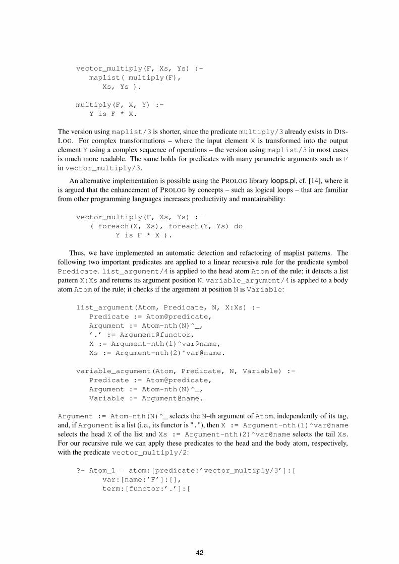
vector_multiply(F, Xs, Ys) :-maplist( multiply(F),

Xs, Ys ).

multiply(F, X, Y) :-Y is F * X.

The version using maplist/3 is shorter, since the predicate multiply/3 already exists in DIS-LOG. For complex transformations – where the input element X is transformed into the outputelement Y using a complex sequence of operations – the version using maplist/3 in most casesis much more readable. The same holds for predicates with many parametric arguments such as Fin vector_multiply/3.

An alternative implementation is possible using the PROLOG library loops.pl, cf. [14], where itis argued that the enhancement of PROLOG by concepts – such as logical loops – that are familiarfrom other programming languages increases productivity and mantainability:

vector_multiply(F, Xs, Ys) :-( foreach(X, Xs), foreach(Y, Ys) do

Y is F * X ).

Thus, we have implemented an automatic detection and refactoring of maplist patterns. Thefollowing two important predicates are applied to a linear recursive rule for the predicate symbolPredicate. list_argument/4 is applied to the head atom Atom of the rule; it detects a listpattern X:Xs and returns its argument position N. variable_argument/4 is applied to a bodyatom Atom of the rule; it checks if the argument at position N is Variable:

list_argument(Atom, Predicate, N, X:Xs) :-Predicate := Atom@predicate,Argument := Atom-nth(N)^_,’.’ := Argument@functor,X := Argument-nth(1)^var@name,Xs := Argument-nth(2)^var@name.

variable_argument(Atom, Predicate, N, Variable) :-Predicate := Atom@predicate,Argument := Atom-nth(N)^_,Variable := Argument@name.

Argument := Atom-nth(N)^_ selects the N–th argument of Atom, independently of its tag,and, if Argument is a list (i.e., its functor is "."), then X := Argument-nth(1)^var@nameselects the head X of the list and Xs := Argument-nth(2)^var@name selects the tail Xs.For our recursive rule we can apply these predicates to the head and the body atom, respectively,with the predicate vector_multiply/2:

?- Atom_1 = atom:[predicate:’vector_multiply/3’]:[var:[name:’F’]:[],term:[functor:’.’]:[

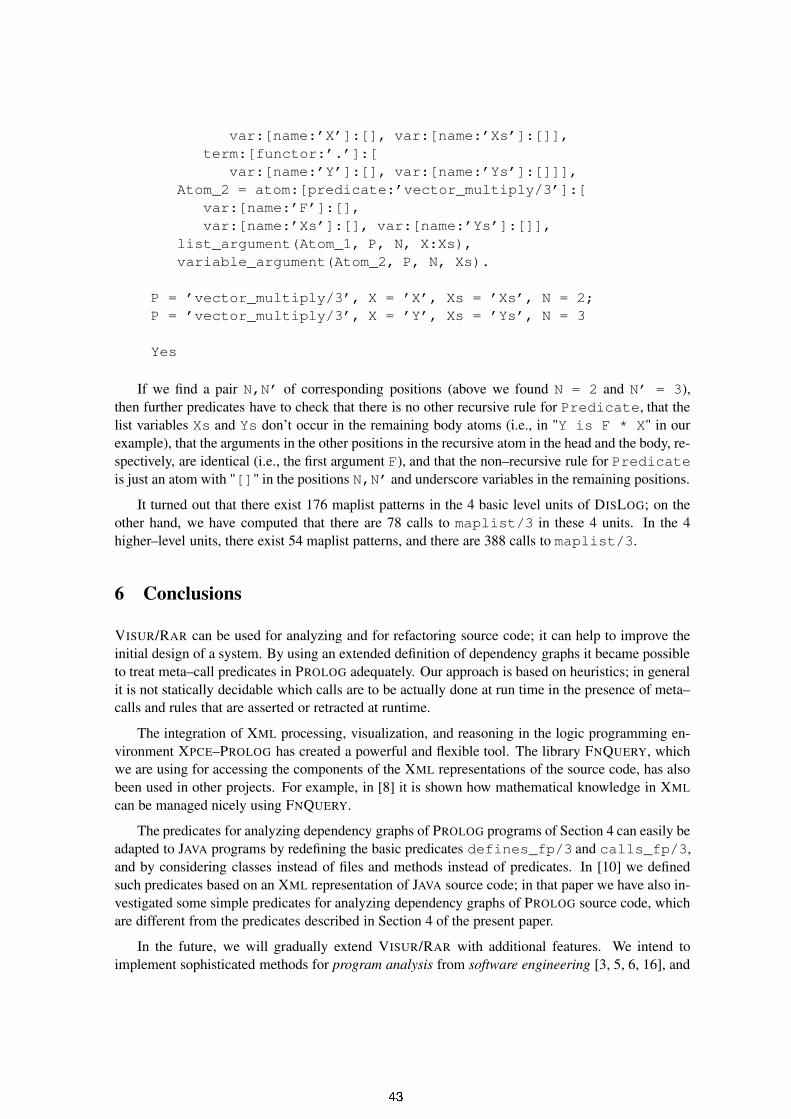
var:[name:’X’]:[], var:[name:’Xs’]:[]],term:[functor:’.’]:[

var:[name:’Y’]:[], var:[name:’Ys’]:[]]],Atom_2 = atom:[predicate:’vector_multiply/3’]:[

var:[name:’F’]:[],var:[name:’Xs’]:[], var:[name:’Ys’]:[]],

list_argument(Atom_1, P, N, X:Xs),variable_argument(Atom_2, P, N, Xs).

P = ’vector_multiply/3’, X = ’X’, Xs = ’Xs’, N = 2;P = ’vector_multiply/3’, X = ’Y’, Xs = ’Ys’, N = 3

Yes

If we find a pair N,N’ of corresponding positions (above we found N = 2 and N’ = 3),then further predicates have to check that there is no other recursive rule for Predicate, that thelist variables Xs and Ys don’t occur in the remaining body atoms (i.e., in "Y is F * X" in ourexample), that the arguments in the other positions in the recursive atom in the head and the body, re-spectively, are identical (i.e., the first argument F), and that the non–recursive rule for Predicateis just an atom with "[]" in the positions N,N’ and underscore variables in the remaining positions.

It turned out that there exist 176 maplist patterns in the 4 basic level units of DISLOG; on theother hand, we have computed that there are 78 calls to maplist/3 in these 4 units. In the 4higher–level units, there exist 54 maplist patterns, and there are 388 calls to maplist/3.

6 Conclusions

VISUR/RAR can be used for analyzing and for refactoring source code; it can help to improve theinitial design of a system. By using an extended definition of dependency graphs it became possibleto treat meta–call predicates in PROLOG adequately. Our approach is based on heuristics; in generalit is not statically decidable which calls are to be actually done at run time in the presence of meta–calls and rules that are asserted or retracted at runtime.

The integration of XML processing, visualization, and reasoning in the logic programming en-vironment XPCE–PROLOG has created a powerful and flexible tool. The library FNQUERY, whichwe are using for accessing the components of the XML representations of the source code, has alsobeen used in other projects. For example, in [8] it is shown how mathematical knowledge in XMLcan be managed nicely using FNQUERY.

The predicates for analyzing dependency graphs of PROLOG programs of Section 4 can easily beadapted to JAVA programs by redefining the basic predicates defines_fp/3 and calls_fp/3,and by considering classes instead of files and methods instead of predicates. In [10] we definedsuch predicates based on an XML representation of JAVA source code; in that paper we have also in-vestigated some simple predicates for analyzing dependency graphs of PROLOG source code, whichare different from the predicates described in Section 4 of the present paper.

In the future, we will gradually extend VISUR/RAR with additional features. We intend toimplement sophisticated methods for program analysis from software engineering [3, 5, 6, 16], and

we want to integrate further refactoring techniques for PROLOG and for JAVA code, which have beendeveloped in [18] for PROLOG.

References

[1] S. Abiteboul, P. Bunemann, D. Suciu: Data on the Web – From Relations to Semi–StructuredData and XML, Morgan Kaufmann, 2000.

[2] S. Ceri, G. Gottlob, L. Tanca: Logic Programming and Databases, Springer, 1990.

[3] S. Diehl (Ed.): Software Visualization: International Seminar, Dagstuhl Castle, Germany,Springer LNCS 2269, 2002.

[4] T. Eiter, N. Leone, C. Mateis, G. Pfeifer, F. Scarcello: A Deductive System for Non–MonotonicReasoning, Proc. Fourth Intl. Conf. on Logic Programming and Non–Monotonic ReasoningLPNMR 1997, Springer LNAI 1265, 1997.

[5] H. Erdogmus, O. Tanir (Eds.): Advances in Software Engineering - Comprehension, Evalua-tion, and Evolution, Springer, 2002.

[6] M. Fowler: Refactoring – Improving the Design of Existing Code, Addison–Wesley, 1999.

[7] M. Hanus, J. Koj: An Integrated Development Environment for Declarative Multi–ParadigmProgramming, Proc. Workshop on Logic Programming Environments WLPE 2001.

[8] B. Heumesser, D. Seipel, U. Güntzer: Flexible Processing of XML–Based MathematicalKnowledge in a PROLOG Environment, Proc. Intl. Conf. on Mathematical Knowledge Man-agement MKM 2003, Springer LNCS 2594.

[9] M. Hopfner, D. Seipel: Reasoning about Rules in Deductive Databases, Proc. 17th Workshopon Logic Programming WLP 2002.

[10] M. Hopfner, D. Seipel, J. Wolff von Gudenberg: Comprehending and Visualising Softwarebased on XML Representations and Call Graphs, Proc. 11th IEEE International Workshop onProgram Comprehension IWPC 2003.

[11] R. Holt, A. Winter, A. Schürr: GXL: Towards a Standard Exchange Format, Proc. WorkingConference on Reverse Engineering WCRE 2000, http://www.gupro.de/GXL/

[12] IBM: The Integrated Development Environment ECLIPSE, http://www.eclipse.org/

[13] M. Kifer, G. Lausen: F–Logic: A Higher–Order Language for Reasoning about Objects, Proc.ACM SIGMOD Conference on Management of Data, 1989.

[14] J. Schimpf: Logical Loops, Proc. Intl. Conference on Logic Programming ICLP 2002.

[15] A. Serebrenik, B. Demoen: Refactoring Logic Programs, Proc. Intl. Conference on Logic Pro-gramming ICLP 2003 (Poster Session).

[16] J. Seemann, J. Wolff von Gudenberg: Pattern–Based Design Recovery of JAVA Software, Proc.Intl. Symposium on the Foundations of Software Engineering 1998.

[17] D. Seipel: Processing XML Documents in PROLOG, Proc. 17th Workshop on Logic Program-ming WLP 2002.

[18] R. Seyerlein: Refactoring in deduktiven Datenbanken am Beispiel des InformationssystemsQualimed, Diploma Thesis, University of Würzburg, 2001.

[19] G. Wagner: How to Design a General Rule Markup Language, Proc. Intl. Workshop on XMLTechnologies for the Semantic Web, XSW 2002.

[20] J. Wielemaker: SWI–PROLOG 5.0 Reference Manual, http://www.swi-prolog.org/J. Wielemaker, A. Anjewierden: Programming in XPCE/PROLOG http://www.swi-prolog.org/

Appendix

We are representing PROLOG programs in XML according to the following DTD, which is suitablefor handling disjunctive logic programs with arbitrarily many head atoms:

<!ELEMENT program (definition*)><!ELEMENT definition (rule*)><!ELEMENT rule (head, body)><!ELEMENT head (atom*)><!ELEMENT body (atom*)><!ELEMENT atom ((term|var)*)><!ELEMENT term (term*)>

<!ATTLIST definition predicate CDATA #required><!ATTLIST rule file CDATA #required><!ATTLIST atom predicate CDATA #required><!ATTLIST term functor CDATA #implied><!ATTLIST var name CDATA #implied>

The arguments of an atom are either terms or variables; constants are represented as terms withoutsubterms, where the constant is stored in the attribute functor.

Demonstration:Debugging Constraint problems with Portable Tools!

Pierre Deransart1, Ludovic Langevine1, and Mireille Ducassé2

1 INRIA Rocquencourt, BP 105, 78153 Le Chesnay Cedex, France{Pierre.Deransart, Ludovic.Langevine}@inria.fr

2 IRISA/INSA, Campus Universitaire de Beaulieu, 35042 Rennes Cedex, FranceMireille.Ducasse@irisa.fr

Presentation of the Demonstration

Many debugging tools for finite domain solvers have been developed in order todebug applications based on finite domain constraints resolution, for example,Grace [2], the Oz Explorer [3], the Oz Constraint Investigator [4], the CHIPglobal constraint visualizer [5], the S-box model [6], the Christmas Tree visual-izer [7] and more DiSCiPl visualization tools [8].

In spite of their very interesting functionalities these tools have a majordrawback, they have a low degree of portability: they are implemented on aspecific platform and the work to port them from one platform to another mayrequire a tremendous effort. From an industrial point of view, one would liketo limit the efforts to port the tools when the same company develops applica-tions with different solver platforms. From a research point of view, one wouldlike to experiment with different tools on different platforms without too muchre-engineering effort.

The previous drawback is all the most daunting that most of the tools aregeneral purpose oriented, i.e. they do not depend on a particular application andthey use quite the same kind of basic information collected in the course ofthe program execution. From this information, more or less complex views aregenerated. In the case of applications, specific animated views are frequentlyproposed, but their animation itself depends on the same basic information.

It is one of the objectives of the OADymPPaC project [1] to realize sucha challenge: to allow several independently developed debugging tools to beused on different solvers. For this purpose an observational semantics whichformalizes relevant aspects of constraint programming and solving has beenintroduced. Then a generic trace schema has been derived which can be used tothen build tracers producing "generic traces" [9]. It is thus possible to developindependently debugging tools whose input data are built from the generic trace.! This work is partly supported by OADymPPaC [1], a French RNTL project.

Several such tools have been independently developed by partners of theOADymPPaC project to visualize very large dynamic structures of constraintproblems. In the meantime several tracers have been implemented whose tracecontains the generic trace events.

We will present in the form of a demonstration the versatility of the ap-proach to analyze, debug and solve a constraint problem. The demonstrationwill especially illustrate how the generic trace helps connect different visualiz-ation tools (in particular adjacency matrices [10] and Ilog Discovery [11]) todifferent platforms (in particular GNU-Prolog [12] and PaLM [13]).

References

1. OADymPPaC: Tools for dynamic analysis and debugging of constraint programs (2001)RNTL project. http://contraintes.inria.fr/OADymPPaC.

2. Meier, M.: Debugging constraint programs. In Montanari, U., Rossi, F., eds.: Proceedingsof the First International Conference on Principles and Practice of Constraint Programming.Number 976 in LNCS. Springer Verlag (1995) 204–221

3. Schulte, C.: Oz Explorer: A Visual Constraint Programming Tool. In: Proceedings of theFourteenth International Conference on Logic Programming (ICLP’97), Leuven, Belgium,The MIT Press (1997) 286–300

4. Müller, T.: Practical investigation of constraints with graph views. In: Principles and Practiceof Constraint Programming – CP 2000. Number 1894 in LNCS, Springer-Verlag (2000)

5. Simonis, H., Aggoun, A., Beldiceanu, N., Bourreau, E.: Complex constraint abstraction :Global constraint visualisation. [8] chapter 12

6. Goualard, F., Benhamou, F.: Debugging Constraint Programs by Store Inspection. [8]chapter 11

7. Bracchi, C., Gefflot, C., Paulin, F.: Combining propagation information and search-treevisualization using opl studio. In Kusalik, A., Ducassé, M., Puebla, G., eds.: Proceedings ofWLPE’01, Cyprus, Cyprus University (2001) 27–39

8. Deransart, P., Hermenegildo, M., Małuszynski, J., eds.: Analysis and Visualisation Tools forConstraint Programming. Number 1870 in LNCS. Springer Verlag (2000)

9. Deransart, P., Ducassé, M., Langevine, L.: A generic trace model for finite domain solvers.In O’Sullivan, B., ed.: Proceedings of User Interaction in Constraint Satisfaction (UICS’02),Cornell University (USA) (2002)

10. Ghoniem, M., Jussien, N., Fekete, J.D.: Visualizing explanations to exhibit dynamic struc-ture in constraint problem. In O’Sullivan, B., ed.: Proceedings of Third Worshop onUser-Interaction in Constraint Satisfaction, UICS’03, Lecture Notes in Computer Science,Springer-Verlag (2003) to appear.

11. Baudel, T., et al: DISCOVERY reference manual (2003) Manufactured and distributed byIlog.

12. Langevine, L., Ducassé, M., Deransart, P.: A Propagation Tracer for GNU-Prolog: fromFormal Definition to Efficient Implementation. In Palamidessi, C., ed.: Proceedings of the19th International Conference on Logic Programming, ICLP’03, Mumbai, India (2003)

13. Jussien, N., Barichard, V.: The PaLM system: explanation-based constraint programming.In: Proceedings of TRICS: Techniques for Implementing Constraint programming Systems,a post-conference workshop of CP 2000, Singapore (2000) 118–133

Proving Termination One Loop at a Time

Michael Codish1 and Samir Genaim2

1 The Department of Computer ScienceBen-Gurion University of the Negev

Beer-Sheva, Israelmcodish@cs.bgu.ac.il

2 Dipartimento di InformaticaUniversita degli Studi di Verona

Verona, Italygenaim@sci.univr.it

Abstract. Classic techniques for proving termination require the iden-tification of a measure that maps program states to the elements of awell-founded domain. Termination is guaranteed if this measure is shownto decrease with each iteration of a loop in the program. This is a globaltermination condition — there exists a measure which is shown to de-crease over all of the loops in the program. In recent years, systemsbased on local termination conditions are emerging. Here, terminationis guaranteed if for every loop there exists a measure which decreasesas execution follows through that loop. In this paper we question therelationship between the two approaches. Reasoning locally is more con-venient. But is the local approach really more powerful? We show thatfor a large class of termination problems the two approaches are equallypowerful. To this end we demonstrate that given local conditions whichsupport a proof of termination, a corresponding global condition can al-ways be constructed. On the one hand, the local conditions are simplerand easier to find. Yet on the other hand, in the local approach one mustconsider a closure operation on loops which may require to consider anexponential number of local conditions.

1 Introduction

Classic techniques for proving termination require the identification of a measurethat maps program states to the elements of a well-founded domain. Terminationis guaranteed if this measure is shown to decrease with each iteration of a loopin the program. Traditionally, the termination condition is global and loops arecharacterized syntactically. Global, because there exists a single measure whichis shown to decrease over all of the loops in the program; and syntactic, becauseloops are defined in terms of the simple cycles in a graph representing, or derivedfrom, the program. Namely, a path with no repeated vertices, except for theinitial and terminal vertex.

In recent years, systems based on local termination conditions and whichcharacterize loops semantically are emerging. Local, because termination is guar-anteed if for every loop there exists a (possibly di!erent) measure which decreasesas execution follows through that loop; and semantic, because loops are charac-terized in terms of program executions. In this approach a loop corresponds toa pair of “program states” at which execution visits the same “program point”.

This paper investigates the relation between the global and local approachesto proving termination. In theory, if there exist local measures to determinetermination then there must exist also a global measure. This follows from thecorrectness of the local approach and from the completeness of the global ap-proach. On the other hand, in practice, analyzers based on the local approachcan often prove termination for programs for which analyzers based on globalfunctions cannot. The question posed is how serious is the rift between the twoapproaches?

We show that for termination analyzers based on the size change terminationprinciple [] or equivalently, on the description of loops in terms of monotonicityconstraints [], the two approaches are of equal power. To this end we illustratehow to construct a global termination measure from a given finite set of localmeasures.

We also show that the construction does not work when loops are describedin a richer language. Hence it is not clear, for the general case what is the relationbetween local and global termination analysis.

In this paper we consider a general setting independently of any particularprogramming language or paradigm. We assume some syntactic notion of a pro-gram point and some semantic notion of a program state. A program point is anode in the parse tree and represents the point just before (or after) the exe-cution of a program statement. A program state associates values for programvariables at a given program point and represents a run-time situation when exe-cution is at the given point. A computation (or program execution) is a, possiblyinfinite, sequence of program states.

To clarify the terminology and to highlight the di!erence between the twocharacterizations of loops consider the following example.

Example 1. Consider the following program fragment, on the left, where p0, p1, p2

and p3 are program points. The graph, given on the right, highlights the flowof control between the program points. The simple cycles in the graph are!p1, p2, p1" and !p1, p3, p1". These are the syntactic loops in the program.

p0: int x = 1, y = 1;p1: while (x + y > 0)

{if (x > y)

p2: { x := x - 1; y := y + 2; }else

p3: { y := y - 1; x := x + 2; }}

For the program above, execution iterates returning to point p1. The pair ofprogram states p1(1, 1) ! p1(3, 0) represents an execution loop because thereis a visit to p1 with x = 1, y = 1 and a subsequent visit with x = 3, y = 0.Similarly, p1(3, 0) ! p1(2, 2) and p1(1, 1) ! p1(2, 2) are also execution loops.The set of all execution loops for the given program is infinite.

In the semantic-based approach to termination analysis, abstract interpre-tation is applied to provide a finite approximation of a program’s (semantic)loops. A concrete semantics that is the basis for the termination analysis of logicprograms is given in [4]. In this semantics the semantic objects are pairs of ini-tial and terminal program states in a computation. The special case where theinitial and terminal states are associated with the same program point indicatesa semantic loop. In the corresponding abstract semantics, loops are described byabstract binary clauses of the form p(x) # !, p(y) where p(x) and p(y) representthe program states at point p before and after executing the loop, and ! is aconstraint describing relations between the sizes of values of the variables of thestates.

Termination analyzers based on abstract interpretation di!er depending onthe type of constraints allowed to appear in !. In [8] the authors use monotonicityconstraints which are binary relations on variables. An equivalent approach ispresented in [7] where the authors represent constraints using, so called, sizechange graphs. In such a graph, nodes correspond to the sizes of the values inthe program states before and after execution of the loop, and labeled edges tobinary relations on variables.

Example 2. Consider the procedure (on the left) defining the Ackerman functionwhere four program points (acker0, . . . , acker3) are indicated using subscripts.

int acker0(int m, int n){ /* restricted for m,n >= 0 */

if (m == 0)return n+1;

else if (n == 0)return acker1(m-1,1);

elsereturn acker3(m-1,acker2(m,n-1));

}

!1 = acker0(x1, x2) !x1 " 0, x2 " 0, y1 " 0, y2 " 0,x1 = y1, x2 > y2, acker0(y1, y2).

!2 = acker0(x1, x2) !x1 " 0, x2 " 0, y1 " 0, y2 " 0,x1 > y1, acker0(y1, y2).

Each recursive call ackeri, with i > 0 gives rise to a loop when execution returnsto acker0. The two abstract binary clauses (on the right) approximate the infinitenumber of concrete execution loops at program point acker0 (for arbitrary non-negative initial values of m and n). The first abstract binary clause representsconcrete loops in which the size of the first argument is invariant and the sizeof the second argument decreases. The second abstract binary clause representsconcrete loops in which the size of the first argument is decreasing.

The following example illustrates the global and local approaches to provingtermination. The formal justification of these are discussed in the next section.

Example 3. The measures f1(acker0(x, y)) = y and f2(acker0(x, y)) = x fromExample 2 decrease respectively for the loop descriptions "1 and "2 in the ex-ample. These are local measures, one for each of the two loops. This provides aproof of termination by the local approach. A global measure can also be identi-fied. Consider the function f(acker0(x, y)) = !f2(acker0(x, y)), f1(acker0(x, y))"which decreases for both loops with respect to the lexicographic ordering onpairs. This provides a proof of termination by the global approach. "

Note that the local approach to proving termination is not necessarily correctwhen loops are represented in the more classic syntactic approach. At least notif we restrict attention only to the simple cycles in the graph.

Example 4. Consider the graph representation of the program from Example 1.The measures f1(p(x, y)) = x and f2(p(x, y)) = y decrease respectively for thetwo cycles in the graph. However the program does not terminate. A proof oftermination in the local approach would have to consider also the non-simpleloop p1p2p1p3p1 for which neither x nor y decreases.. "

Reasoning locally about loops does have advantages. Local termination mea-sures are often simpler. They are easier to identify, by the human user as well aswhen aiming for automated proofs. For example, there are many cases whereproofs based on local measures involve linear functions while correspondingglobal measures involve tuples ordered lexicographically. As a consequence, an-alyzers implemented to use linear techniques are more successful when based onlocal instead of global termination conditions.

2 Preliminaries

This section presents the local approach to proving termination, recalls the clas-sic justification for the global approach and explains why the justification of thelocal approach is problematic.

To simplify the presentation, we assume that the (syntactic) loops of a pro-gram P are given as abstract binary clauses, for example a program point p(where the execution iterates) is described using p(x) # !, p(y), where x is thevalues of the program’s variables (a state) when entering the loop, y is the statewhen revisiting the loop, and ! is the size-relations between the two states.Formally speaking, (abstract) binary clauses are defined as follows.

Definition 1 (Abstract binary clauses). An abstract binary clause C is aclause of the form p(x) # !, p(y) where x and y consists of distinct tuples ofvariables and ! are linear constrains over a well-founded domain D = !D,<"that involve only the variables of x and y only. Moreover, we assume that !contains the implicit constraint {v $ 0|v % vars(x) & vars(y)}.

Often, the constraint domain D that used to describe a binary clause, is fur-ther restricted to contain only monotonicity constraints [8]. These are conjunc-tions of binary relations (<,',=) between pairs of variables. This restriction,

and in general the choice of D, is sometimes crucial to proving termination asshow in the following example.

Example 5. Consider the following binary clause p(x1, x2) # !, p(y1, y2) where! ( [y1 = 2 ) x2 + 1 * x1 = 3 ) y2 + 2] and assume it is the only loop in theprogram. It is easy to verify that f(a1, a2) = a1 + 3 ) a2 is decreasing for thisbinary clause, i.e ! |= f(y1, y2) > f(x1, x2), hence the program terminates. But,restricting ! to monotonicity constraints results in !! ( [y1 > x2, x1 < y2], andthere is no f such that [y1 > x2, x1 < y2] |= f(y1, y2) > f(x1, x2). Therefore,with this restriction we cannot prove termination.

Loop descriptions involving monotonicity constraints can also be representedas size change graphs [7] where directed edge from x to y indicates a constraintx > y, and non-directed edge indicates a constraint x $ y.

Example 6. Consider the loop descriptions from Example 2. These will be de-picted by the size change graphs.

The vertices on the top of the graph correspond to those in the head of the binaryclause and those on the bottom to the variables in the body of the clause.

The correctness of the local approach to proving termination relies on the factthat implicit loops are made explicit first, only then we can claim termination ifwe find (possibly di!erent) decreasing measures for each of these loops. Makingthe implicit loops explicit is done by closing the set of (syntactic) binary clausesunder compositions, where the composition of two loops is defined as follows.

Definition 2 (Composing loops). Let "1 = p(x) # !1, p(y) and "2 = p(y) #!2, p(z) be (renaming of) programs loops descriptions (which do not share vari-ables except those in y). The composition of "1 and "2 is defined as "1 + "2 =p(x) # ,y. !1 * !2, p(z).

The following example illustrates the composition of two loops. Note theprojection of the variables (by ,y).

Example 7 (Composing loops). Consider the loop descriptions "1 and "2 fromExample 2. Observe that "1 + "1 = "1, "1 + "2 = "2 + "1 = "2, and "2 + "2 = "2.For example assuming that "1 = p(x1, x2) # [x1 = y2, x2 > y2], p(y1, y2) and"2 = p(y1, y2) # [y1 > z1], p(z1, z2), then the composition "1 + "2 results in"1 = p(x1, x2) # [x1 > z1], p(z1, z2) (which is a variant of "2) as illustrated inthe following diagram:

It is important to note that closing a set of loop descriptions under compo-sition can introduce an exponential number of additional descriptions [7].

The following proposition provides conditions when we can claim terminationbased on the local approach.

Proposition 1. Let P be a logic program, p a program point at which the exe-cution can loop, and Lp a closed set (under composition) of binary clauses con-structed from the syntactic loops of p, then: If for each " ( p(x) # !, p(y) % Lp

there exists a function f! which maps states to a well-founded domain D = (D,<)such that ! |= f(p(y)) < f(p(x)) then p terminates. The set of all such functionsf! is denoted by Cp.

Before discussing the formal justification of the local approach, let us recallthat for the more classic, global approach. The global approach is the specialcase where in Proposition 1 the set Cp consists of a single function f whichdecreases for all of the loop descriptions associated with program point p. Theproof of correctness for this case is classic. In brief, consider that if there wereto exist an infinite computation for P then there would be a program point pvisited infinitely often in that computation. Denote the corresponding sequenceof visits at p as

p1 ! p2 ! · · · ! pk ! · · ·

Each pair pi ! pi+1 is a concrete loop described by one of the loop descriptionsfor p and the function f decreases for that pair. But f maps states to a wellfounded domain and cannot decrease infinitely often. Hence there cannot existan infinite computation.

For the local approach this argument no longer holds as pairs of states pi !

pi+1 may be associated with di!erent functions and the pairs for which onefunction decreases may cause another to increase.

In some cases it is easy to work around this type of problem, for examplewhen there is some regularity in the loops describing the corresponding transi-tions from program point p to program point p. For instance, if we consider acomputation in which the concrete loops are described by "1 and "2 alternatingas illustrated (the transitions are labeled by the corresponding loop description):

p!1! p

!2! p

!1! p

!2! p

!1! p

!2! p

!1! p

!2! · · ·

then we also have an infinite computation of the form

p!1"!2! p

!1"!2! p

!1"!2! p

!1"!2! · · ·

and there is a function f associated with the loop "1 + "2 which cannot decreaseinfinitely often.

But in general one cannot expect to always find such regularity, as for exampleillustrated by the infinite computation of the form

p!3! p

!1! p

!4! p

!1! p

!5! p

!9! p

!2! p

!6! · · ·

where the loop descriptions correspond to the digits of the constant #.A formal justification of the local approach to proving termination is pre-

sented in [5]. The proof is based on an application of Ramsey’s theorem [9]. Wepresent here the proof of correctness for termination reasoning about individualloops. The proof is set as an application of Ramsey’s Theorem [9]. It is essen-tially the same as that presented by Dershowitz et al.DLSS01 for logic programsin [5].

Theorem 1. Let P be a program, and suppose we proved termination of P usingthe local approach as described in Proposition 1. Then P terminates.

The proof is by contradiction as an application of Ramsey’s Theorem [9].

Ramsey’s Theorem: Let A =!!a, b"

""a, b % IN and a < b#, C be a finite set

of colors and let F : A-.C be a function associating the elements of A withcolors from C. Then, there is a color f%C and an infinite set X / IN such thatF(!a, b") = f for each a, b % X for which a < b.

Proof. (of Theorem 1)Assume in contradiction that P has an infinite computation. This implies thatthere is a program point p which is visited infinitely often. Denote the corre-sponding sequence of visits at p as

S = p1 ! p2 ! · · · ! pk ! · · ·

To apply Ramsey’s Theorem we should fix a finite set of colors C and a mappingF of elements of A =

!!a, b"

""a, b % IN and a < b#

to colors. We take as colorsthe set of functions Cp prescribed by Proposition 1. To fix the mapping F , wenote that each pair of visits pa and pb with a < b denotes a (semantic) loop atp and is hence associated with a corresponding loop description and a functionfi % Cp. Ramsey’s Theorem implies the existence of an infinite subsequence of Sof the form

S ! = pi1 ! pi2 ! · · · ! pik ! · · ·

for X = {i1, i2, . . . , ik, . . .} such that the loop corresponding to any pair of visitspia and pib with a < b decreases with respect to the same function f % Cp. Butsince f maps states to a well-founded domain, this is a contradiction. "

3 When Local Meets Global

In this section we illustrate that for termination analysis based on monotonicityconstraints (or equivalently, on the size change principle), the local and globalapproaches are of equivalent power. One direction of the argument is straight-forward, as a global measure for termination is also a local measure. To showthe other direction, we show that if we can prove termination in the local ap-proach then we can also construct a global termination condition. This providesan alternative justification of the local approach, for the given class of case ofmonotonicity constraints.

Finding local functions for termination is easy. In [8] the authors show thatif adding the “up arrows” in the graphs introduces a cycle (with at least onestrict decrease then there exists a function. in [4], the authors add to each ! theconstraints xi < yi and check that the resulting constraint is inconsistent, andin [7] the authors prove that it is su"cient to find a single down arrow in all sizechange graphs that are idempotent (in the closure). The question is how to finda suitable global function.

Example 8. Consider the three loop descriptions for i % {1, 2, 3}

!i # p(x1, x2, x3) ! "i, p(y1, y2, y3)

with !1 = x1 > y1, x2 > y1, !2 = x1 $ y2, x2 $ y2, x3 > y3 and!3 = x1 $ y2, x2 > y2 where all of the variables are assumed to be non-negative.In the local approach a proof of termination is obtained choosing the followingfunctions corresponding to the three loops: f1(p(x, y, z)) = x, f2(p(x, y, z)) = zand f3(p(x, y, z)) = y. In the global approach a proof is obtained choosing aglobal function f(p(x, y, z)) = !min(x, y), y, z" with the standard lexicographicordering.

Definition 3 (Monotonic functions for a set of loops). Let Lp be a finiteset of loop descriptions with corresponding functions Cp mapping states to well-founded domains such that for each " = p(x) # !, p(y) % Lp and correspondingfunction f! : State . D it holds that ! |= f(p(y)) < f(p(x)). We say that Cp ismonotonic for L if for any composition " = "1 + · · · + "k of (a subset of) loopsfrom Lp, the function f! associated with the loop " satisfies: (1) 01 ' i ' k.!i |=f!(p(x)) $ f!(p(y)); and (2) ,1 ' i ' k.!i |= f!(p(x)) > f!(p(y)).

"

Example 9. Consider again the three loops from Example 8.

1. The set of functions f1(p(x, y, z)) = x, f2(p(x, y, z)) = z and f3(p(x, y, z)) =y is note monotonic for these three loops. Observe that "3 + "2 + "1 = "1 andf1 does not decrease (even weakly) for "2.

2. The single function f1(p(x, y, z)) = f2(p(x, y, z)) = f3(p(x, y, z)) = !min(x, y), y, z"is monotonic for the three loops.

Theorem 2. Let Cp be a monotonic set of functions for loop descriptions L.Then there exists an ordered tuple !f1, . . . , fk" of functions from Cp such thatthe function f defined by f(s) = !f1(s), . . . , fk(s)" decreases globally for all ofthe loop descriptions in Lp with respect to the corresponding lexicographic order.Moreover, this ordered tuple can be constructed with time complexity O(|Lp|2)."

The algorithm presented in Figure 1 constructs the required tuple of functionsfrom Cp and provides the proof. The basic idea is that if we compose a monotonicset of local loop descriptions from Lp then we identify a function from Cp whichdecreases when passing through at least one of the composed loops but neverincreases when going through these loops. Hence this function may be placed tothe right of these functions in the tuple we are constructing.

(0) S = Lp and # = $(1) WHILE ( S %= $ ) DO(2) ! = compose loops(S) \* compose in any order *\(3) IF ( ! & S ) THEN(4) # = #.f!

(5) S = S \ {!}(6) ELSE(7) S = { p(x) ! ", p(y) & S | " %|= f!(p(x)) > f!(p(y)) }(8) \* remove from S all loops that decrease for f! *\(9) DONE

Fig. 1. Constructing a global decreasing measure

The algorithm proceeds as follows: We start (at line 0) with S = Lp and anempty tuple #. At each iteration of the while loop (lines 1-9) we compose theloops of S (line 2). If the result " is an element of S then we add it to the right inthe tuple # (line 4) and remove it from S (line 5). Otherwise, if " 1% S, then (sinceS is monotonic) there must be at least one loop "! ( p(x) # !, p(y) % S suchthat ! |= f!(p(x)) > f!(p(y)). This means whenever traversing a loop describedby "!, both of the functions f!! and f! decrease. Hence, we can remove any such"! from S (lines 7-8).

The correctness of the algorithm stems from the following: (1) At each stepwe remove at least one loop from S so the algorithm terminates; (2) The factthat S is monotonic together with lines 3-5 guarantees that whenever a functionfi (in the tuple) decreases, any function to its left either decreases or remainsinvariant; and (3) lines 7-8 guarantees that for each loop description there is atleast one corresponding function in the tuple.

Since we remove at least one loop at each iteration, the complexity of thealgorithm is O(|Lp|2) – we count the number of times we compose two loops(the basic step of compose loops) plus the operations on sets at lines 4, 7 and 8.

Example 10. Consider the following abstract loop descriptions (where all of thevariables are assumed to be non-negative).

!1 = p(x1, x2, x3) ! x1 > y1, x2 > y2, p(y1, y2, y3).!2 = p(x1, x2, x3) ! x1 = y1, x3 > y3, p(y1, y2, y3).!3 = p(x1, x2, x3) ! x1 > y1, p(y1, y2, y3).

As local functions associated with "1, "2 and "3 we take f1(p(x, y, z)) = x,f2(p(x, y, z)) = z, f3(p(x, y, z)) = x. The algorithm starts with S = {"1, "2, "3}and proceeds as follows:

1. "1 + "2 + "3 = "3, so we take f3 as the first function in the tuple and remove"3 from S.

2. "1 + "2 = "3 and "3 is not in S. We see that f3 decreases on "1 (as well as on"3), so we remove "1 from S.

3. "2 is the only remaining loop in S so we take f2 as the next function in thetuple and remove "2 from S.

The function f(s) = !f3(s), f2(s)" decreases (globally) for all of the loops in theoriginal description. "

It still remains unclear how to find a suitable set of functions which is mono-tonic for the given loops. For the special case where all binary constraints arebetween the same arguments (xi with yi), the task is more simple.

Lemma 1. If all of the constraints occurring in the loop descriptions Lp aremonotonicity constraints of the form xi < yi or xi ' yi (namely between thesame argument positions) then Lp is a monotonic set of loops. "

To extend the result for the full class of monotonicity constraints we needto consider all local functions of the form mini#I(xi), maxi#I(xi), sumi#I(xi)for I a subset of the arguments in the state. In addition, we do not want tofix from the start a set of functions which is monotonic for the full set of loopdescriptions, but rather at each stage in the algorithm of Figure 1 we need a setof functions monotonic for the loops in the set S (those which still remain inthe game). Finally, consider the ith iteration of the algorithm and assume thatthe set of functions F have already been introduced to the tuple # and that theloop descriptions left are in S. Hence, by the construction the functions in Fremain invariant for the loops in S (otherwise they would have been removed ina previous stage of the algorithm). We may take this into account when lookingfor the monotonic set of functions in the next iteration for S.

4 The General Case

Theorem 2 does not hold for the general case for example, when loops are de-scribed are expressed using linear constraints (but not necessarily monotonicityconstraints). We illustrate this by example.

In the following example, loop descriptions are given in a richer domain al-lowing linear constraints. In this case it is not obvious to detect a global functionwith which to prove termination. Existing analyzers based on the global approachdo not succeed to provide the proof.

Example 11. Consider the following three loop descriptions where the variablesxi, yi, zi are assumed to be non-negative:

!1 # p(x1, y1, z1, k1, l1) ![k1 = k2, l1 = l2, x1 > x2, k1 = 0, l1 = 0],p(x2, y2, z2, k2, l2).

!2 # p(x1, y1, z1, k1, l1) ![k1 = k2, l1 = l2, y1 > y2, x1 > x2 + k1, k1 + l1 = 0],p(x2, y2, z2, k2, l2).

!3 # p(x1, y1, z1, k1, l1) ![k1 = k2, l1 = l2, z1 > z2, x1 = x2 + l1, k1 = l1],p(x2, y2, z2, k2, l2).

With the local approach we can prove termination taking f!1(p(x, y, z, k, k)) = x,f!2(p(x, y, z, k, l)) = y and f!3(p(x, y, z, k, l)) = z. Composing any two (di!er-ent) loops results in "1. So, the set of abstract binary clauses is closed un-der composition. But there is no permutation !fi1 , fi2 , fi3" such that f(s) =!fi1(s), fi2(s), fi3(s)" is guaranteed to decrease globally on all three loops. "

5 Conclusion

This paper poses a question concerning the relation between the global and localapproaches to proving termination. We show that in many cases we can combinelocal termination conditions into a tuple of functions ordered such that the tuplefunction decreases globally with respect to the lexicographic ordering.

While the results of the paper strengthen our belief that reasoning with localconditions has clear practical advantages, still, we lack the hard evidence thatthe local approach is more powerful than the global one or not. This is the e!ortof our ongoing research.

The very elegant result of Theorem 1 is not well known and is due to Der-showitz et al. [5]. It has subsequently been worked out independently by othersworking on the analysis of termination using local conditions as described in [3],[1] and [6].

Ben-Amram in [2] presents a transformation so that any program P for whichthe local approach works based on monotonicity constraints (or the size changeprinciple) is transformed to a semantically equivalent program P $ with the sametermination behavior for which termination can be identified in terms of lexico-graphic descent. This is the case handled by the special case of Lemma 1.

References

1. Maurice Bruynooghe, Michael Codish, John Gallagher, Samir Genaim, and WimVanhoof. Termination analysis through combination of type based norms, May2003.

2. Amir M. Ben-Amram. General size-change termination and lexicographic descent.In Torben Mogensen, David Schmidt, and I. Hal Sudborough, editors, The Essenceof Computation: Complexity, Analysis, Transformation. Essays Dedicated to NeilD. Jones, volume 2566 of Lecture Notes in Computer Science, pages 3–17. Springer-Verlag, 2002.

3. Michael Codish, Samir Genaim, Maurice Bruynooghe, John Gallagher, and WimVanhoof. One loop at a time. In 6th International Workshop on Termination(WST 2003), June 2003.

4. Michael Codish and Cohavit Taboch. A semantic basis for the termination analysisof logic programs. The Journal of Logic Programming, 41(1):103–123, 1999.

5. N. Dershowitz and N. Lindenstrauss and Y. Sagiv and A. Serebrenik. A GeneralFramework for Automatic Termination Analysis of Logic Programs. Applicable Al-gebra in Engineering, Communication and Computing, Springer-Verlag Heidelberg,12(1-2):117–156, 2001.

6. Chin Soon Lee. Program Termination Analysis and Termination of O!ine PartialEvaluation. PhD thesis, University of Western Australia, August 2002.

7. Chin Soon Lee, Neil D. Jones, and Amir M. Ben-Amram. The size-change principlefor program termination. ACM SIGPLAN Notices, 36(3):81–92, 2001.

8. N. Lindenstrauss and Y. Sagiv. Automatic termination analysis of logic programs.L. Naish, editor. Proceedings of the Fourteenth International Conference on LogicProgramming, pages 63–77. Leuven, Belgium, 1997. The MIT Press.

9. F.P. Ramsey. On a problem of formal logic. In Proceedings London MathematicalSociety, volume 30, pages 264–286, 1930.

Hasta-La-Vista: Termination Analyser for LogicPrograms

Alexander Serebrenik, Danny De Schreye

Department of Computer Science, K.U. LeuvenCelestijnenlaan 200A, B-3001, Heverlee, Belgium

E-mail: {Alexander.Serebrenik,Danny.DeSchreye}@cs.kuleuven.ac.be

Abstract. Verifying termination is often considered as one of the most import-ant aspects of program verification. In this paper we present Hasta-La-Vista—anautomatic tool for analysing termination of logic programs. To the best of ourknowledge, Hasta-La-Vista is unique in being able to prove termination of pro-grams depending on integer computations.

1 Introduction

Proving termination is often considered as an important aspect of program veri-fication. Logic programming languages, allowing us to program declaratively,increase the danger of non-termination. Therefore, termination analysis receivedconsiderable attention in logic programming (see, e.g., [8, 14, 27]). Unfortu-nately, most work on termination analysis is restricted to pure logic programsand thus many interesting real-world examples are left out of consideration. Ar-itmetic is a case in the point: while almost every real-world program containsa numerical part, most other works modelled it by 0 and the successor func-tion. Therefore, in order to bridge the gap between programming practice andexisting termination analysers, real-world programming techniques should beconsidered.

In this paper we present Hasta-La-Vista1 — a powerful tool for analysingtermination of logic programs with integer computations. While such programsare very common in real-world programming, until recently they mostly re-mained a terra incognita for the termination research community. In fact, noneof the existing termination analysers we are aware of (TermiLog [22], Termin-Web [8], TALP [28], and cTI [26]) is powerful enough to prove termination evenof the simplest integer computations such as the following program:Example 1.

p(X)! X < 7, X1 is X+1, p(X1).

1 Hasta la vista, baby! The Terminator in [6]

Assuming the left-to-right selection rule of Prolog, this program terminates forqueries p(X), for all integer values of X . !Our approach is based on transforming a program in a way that allows integ-rating and extending techniques originally developed for analysis of numer-ical computations in the framework of query-mapping pairs [15] with the well-known framework of acceptability [14].

Furthermore, our approach is not limited to proving termination, but canalso infer termination. More precisely, we will be inferring conditions that, ifimposed on the queries, will ensure that the queries will terminate. Inference oftermination conditions was studied in [18, 26]. Unlike termination conditions in-ferred by these approaches, stated in terms of groundness of arguments (calls toappend terminate if either the first or the third argument is ground), our tech-nique produces conditions based on numerical domains of the arguments asshown in Example 2. Combining the approaches to infer both kinds of con-ditions is considered as a future work.

Example 2. Consider the following program.

q(X ,Y )! X > Y, Z is X"Y, q(Z,Y ).

Queries of the form q(arg1,arg2), where arg1 and arg2 are integers, terminatewith respect to this program if either arg1 # arg2 or arg1 > arg2 and arg2 > 0.This is exactly the termination condition we will infer. !

The rest of the paper is organised as follows. In the next section we presenta general overview of the system. The presentation is kept on the intuitive level,more formal results can be found in [33]. Section 3 contains detailed discussionof an experimental evaluation of the method. In Section 4 we discuss furtherextensions, such as proving termination of programs depending on numericalcomputations as well as symbolic ones. We summarise our contribution in Sec-tion 5, review related work and conclude.

2 System architecture

In this section we present an overview of the system architecture and illustratethe working of main components by analysing Example 2.

Conceptually, Hasta-La-Vista consists of three main parts: transformation,constraint generation and constraint solving. As a preliminary step, given a pro-gram and a set of atomic queries, type analysis of Janssens and Bruynooghe [20]computes the call set. We opted for a very simple type inference technique thatprovides us only with information whether an argument is integer or not. More

refined analysis can be used. For instance, the technique presented in [21] wouldhave allowed us to know whether some numerical argument belongs to a certaininterval. Alternatively, the integer intervals domain of Cousot and Cousot [11]might have been used. For our running example type analysis establishes thatall calls that will be generated are of the form q(int, int).

Based on the results of the type analysis the system approximates whethertermination of the given program can be dependent on the integer computation.It should be noted that there are programs, such as quicksort, that use arithmeticbut whose termination behaviour is not dependent on their arithmetic part. Thisis not the case, however, for Example 2, since the integer assignment operator(is) is used to produce a value in the recursive call to q.

If Hasta-La-Vista suspects that termination depends on arithmetic, the ad-orning transformation [33] is applied. The aim of the transformation is to splitthe domain of calls in order to allow each one of the cases to be analysed separ-ately. In this way we discover bounded integer arguments and make the boundsexplicit. Intuitively, we are interested in bounded arguments, since if, for ex-ample, a variable x is known to be bounded from above by n, then n"x is alwayspositive and thus, it can be used as a basis for a definition of a level-mapping(a function from the set of atoms to the naturals). Similarly, if a variable x isbounded from below by n, x" n is always positive and thus, can be used as abasis for a definition of a level-mapping. To illustrate the transformation con-sider the following example.

Example 3. We are interested in proving termination of the set of queries {p(n) |n is an integer} with respect to the following program:

p(X)! X > 1, X < 100, X1 is "X2, p(X1).p(X)! X <"1, X >"100, X1 is X2, p(X1).

Let arg1 denote the first argument. The first clause is applicable, i.e., theclause is selected and the test is passed, if the constraint c1 $ 1 < arg1 < 100holds for p(X). Similarly, the second clause is applicable if c2$"100< arg1 <"1 holds for p(X). Thus, termination of p(X) for c3 $ (arg1 # "100%"1 #arg1 # 1% arg1 & 100) is trivial. We call c1,c2 and c3 adornments and denotethe set of adornments Ap. In general, adornments are constructed as (disjunc-tions of) conjunctions of comparisons appearing in the bodies of the clauses.Formally, Ap, computed by Hasta-La-Vista, is the set of all conjunctions 'ni=1di,where di is either a conjunction of comparisons appearing in the body of a clauseor its negation.

It should be noted that if c1 holds and the first clause is applied, then eitherc2 or c3 hold for the recursive call. We use this observation and specialise the

program with respect to c1,c2 and c3 (cf. [39]). The following program is ob-tained:

pc1(X)! X > 1, X < 100, X1 is "X2, "100< X1, X1<"1, pc2(X1).pc1(X)! X > 1, X < 100, X1 is "X2,

(X1#"100;("1# X1, X1# 1);X1& 100), pc3(X1).pc2(X)! X <"1, X >"100, X1 is X2, 1< X1, X1< 100, pc1(X1).pc2(X)! X <"1, X >"100, X1 is X2,

(X1#"100;("1# X1, X1# 1);X1& 100), pc3(X1).

Observe that in our example there are no clauses defining pc3 in the specialisedprogram since c3 is not consistent with tests in the clauses.

For the specialised program the following holds. In case c1, arg1 is boundedby 1 and 100, in case c2, it is bounded by "100 and "1. This information isessential for proving termination. !

Similarly, Hasta-La-Vista discovers that there are two adornments relevantfor q in Example 2: arg1 # arg2 and arg1 > arg2. In the former case the pro-gram clause is not applicable and termination is trivially established. In the lat-ter case termination has to be proved. Observe that the second argument of q isbounded from above by its first argument, and thus arg1"arg2 is a natural num-ber. Extending the constraints-based approach of Decorte et al. [14] we define alevel-mapping for q(t1, t2) asWq1>q2 · (t1" t2) if t1 > t2 and as zero, otherwise,whereWq1>q2 is a parameter ranging over a finite domain of natural numbers. Ingeneral, a level mapping is a linear combination of differences corresponding toinequalities appearing in adornments.

In order to prove termination, the acceptability condition requires the level-mapping to decrease from the call unified with the head of the clause to the cor-responding call to the recursive body subgoal. This condition can be translatedinto a set of constraints over two kinds of variables: parameters and numericalvariables. For our example the following constraint is obtained:

Wq1>q2 · (X"Y ) >Wq1>q2 · ((X"Y )"Y ),

that is, Wq1>q2 ·Y > 0 should hold. In [14] variables such as X and Y aboveshould be interpreted as sizes of terms ranging over the naturals. In our case,they correspond to the integer variables of the program, so we do not know apriori that they are natural numbers.

This set of constraints is solved with respect to the parameters. If one canfind the parameter values such that the set of constraints is satisfied for all pos-sible values of the numerical variables, termination is reported for all queries.

If for some parameter values one can find additional constraints on the numer-ical variables corresponding to the query arguments such that the original setof constraints is satisfied, we infer termination for queries satisfying these addi-tional constraints. Finally, if none of the previous cases is applicable possibilityof non-termination is suspected. In our case, to conclude the proof we observethat sinceWq1>q2 & 0, then we have Y > 0 andWq1>q2 > 0. Variable Y appearsin the head of the clause, i.e., Y > 0 can be viewed as a constraint on the query.This completes the analysis for the case arg1 > arg2. Recalling our earlier ob-servations we report termination for (arg1 # arg2)% (arg1 > arg2 ' arg2 > 0).Formally, the algorithm is sketched in Figure 1.

Let P be a homogeneous program, let S be a single predicate set of atomic queries and let q berel(S).

1. For each p( q construct a guard-tuned set Ap.2. Adorn P with respect to q and

!p(qAp.

3. Let A= {c | c)Aq, for all p such that qc * p: p is not recursive in Pa}. Let cond1 ="c)A c.

Let cond2 ="c)Aq,c +)A c.

4. Let S, be {c(Q)'Qc | c ) Aq,c +) A,c(Q)'Qc ) Sa}.5. Define the symbolic counterparts of level mappings and interargument relations.6. Let Σ be a set of constraints on the symbolic variables, following from rigid acceptability of

S, with respect to Pa and the validity of interargument relations.7. Solve Σ with respect to the symbolic variables.

(a) Solution of Σ doesn’t produce extra constraints on variables.Report termination for true.

(b) Solution of Σ produces extra constraints on integer variables, appearing in the heads ofthe clauses.

Conjunct these constraints to termination condition cond2.Report termination for cond1% cond2.

(c) There are no solutions or integer variables, constrained by the solution of Σ, do notappear in the heads of the clauses

Report termination for cond1.

Fig. 1. The Termination Inference Algorithm

One can show that for our running example the termination condition in-ferred is optimal, i.e., if it is not satisfied the computation will proceed infin-itely. However, the undecidability of the termination problem implies that noautomatic tool can always guarantee optimality.

Example 4. Consider the following program.

q(X ,Y )! X > Y, Z is X"Y, Y1 is Y +1, q(Z,Y1).

We would like to study termination of this program with respect to {q(z1,z2) |z1,z2 are integers}. Our algorithm infers the following termination condition:arg1 # arg2% (arg1 > arg2'arg2 & 0). This is a correct termination condition,but it is not optimal as q(z1,z2) terminates, in fact, for all values of z1 and z2,i.e., the optimal termination condition is true. !

3 Experimental evaluation

We have tested our system on a number of examples. First of all, we consideredinteger examples from two textbooks’ chapters dedicated to programming witharithmetic, namely, Chapter 8 of Sterling and Shapiro [37] and Chapter 9 ofApt [1]. These results are summarised in Table 1. We can prove termination ofall the examples presented for all possible values of the integer arguments, thatis, the termination condition inferred is true. Next, we’ve collected a number ofprograms from different sources: mostly from textbooks and benchmark collec-tions. Table 2 presents timings and results for these programs. Again, termina-tion of almost all programs can be shown for all possible values of the integerarguments. We believe that the reason for this is that most textbooks authors aimto teach how to write good software and always keep termination in mind. Fi-nally, Table 3 demonstrates some of the termination conditions inferred by oursystem. We can summarise our results by saying that the system turns out to bepowerful enough to analyse correctly a broad spectrum of programs, while thetime spent on the analysis never exceeds 0.30 seconds. In fact, for almost 90%of the integer programs results were obtained in less than 0.10 seconds. Observethat for some examples the time needed to perform the analysis was too smallto be measured exactly. These cases are indicated by 0.00 in the Time column.

The core part of the implementation was done in SICStus Prolog (version3.10.0), using its CLP(FD) and CLP(Q) libraries. The type inference of Janssensand Bruynooghe [20] was implemented in MasterProLog (release 4.1i). Testswere performed on Intel R-Pentium R-4 with 1.60GHz CPU and 260Mbmemory,running 2.4.20-pre11 Linux.

In Tables 1–3, the following abbreviations are used:

– Ref: reference to the program;– Name: name of the program;– Queries: atomic queries of interest, where the arguments are denoted

• c, if the argument is a character;• i, if the argument is an integer;• li, if the argument is a list of integers;• lp, if the argument is a list of pairs of integers;• t, if the argument is a binary tree, containing integers;

Table 1. Examples from [37, 1]

Ref Queries Time Ref Queries TimeExamples of Sterling and Shapiro [37] Examples of Apt [1]

8.1 greatest common divisor(i, i, v) 0.01 between between(i, i, v) 0.028.2 factorial(i, v) 0.01 delete delete (i, i, v) 0.038.3 factorial(i, v) 0.02 factorial fact(i, v) 0.018.4 factorial(i, v) 0.02 in tree in tree(i, t) 0.008.5 between(i, i, v) 0.02 insert insert(i, t, v) 0.018.6a sumlist(li, v) 0.00 length1 length(li, v) 0.008.6b sumlist(li, v) 0.01 maximum maximum(li, v) 0.008.7a inner product(li, li, v) 0.00 ordered ordered(li) 0.018.7b inner product(li, li, v) 0.01 quicksort qs(li, v) 0.068.8 area(lp, v) 0.02 quicksort acc qs acc(li, v) 0.058.9 maxlist(li, v) 0.02 quicksort dl qs dl(li, v) 0.088.10 length(v, li) 0.01 search tree is search tree(t) 0.038.11 length(li, v) 0.01 tree minimum minimum(t, v) 0.018.12 range(i, i, v) 0.02

• v, if the argument is a variable;– Time: time (in seconds) needed to analyse the example;– T (in Table 2): termination behaviour:

• T means that the termination condition inferred is true, i.e., computa-tion of any query from the specified set with respect to a given programterminates;

• N+ means that the termination condition inferred is false and indeedcomputation of a query from the specified set with respect to a givenprogram does not necessarily terminate;

• T. means that the termination condition inferred is true, but a transform-ation was required as a preliminary step (see further);

– Condition (in Table 3): termination condition (other than true and false) in-ferred by the system.

A surprising result was the discovery of non-terminating examples in Prologtextbooks. The first one, by Coelho and Cotta [9], should compute an nth powerof a number.

exp(X ,0,1).exp(X ,Y,Z)! even(Y ), R is Y/2, P is X .X , exp(P,R,Z).exp(X ,Y,Z)! T is Y "1, exp(X ,T,Z1), Z is Z1.X .

even(Y )! R is Y mod 2, R= 0.

The termination condition inferred by our system is false. Indeed, this is theonly termination condition possible, since, for any query exp(arg1,arg2,arg3)

Table 2. Various examples

Name Ref Queries Time Tdldf [3] depthfirst2(c, v, i) 0.03 Texp [9] exp(i, i, v) 0.05 N+fib [5] fib(i, v) 0.12 Tfib [12] fib(i, v) 0.27 Tfib [29] fib(i, v) 0.03 T.forwardfib [3] fib3(i, v) 0.02 Thanoi [16] hanoi(i,v,v,v) 0.18 Tinterval [35] interval(i,i,v) 0.02 Tmoney [5] money(v, v, v, v,v, v, v, v) 0.13 Tmortgage [24] mortgage(i,i,i,i,v) 0.02 T.oscillate Example 3 p(i) 0.15 Tp [15] p(i) 0.01 Tp32 [19] gcd(i, i, v) 0.03 Tp33 [19] coprime(i, i) 0.04 Tp34 [19] totient phi(i, v) 0.08 Tprimes [7] primes(i, v) 0.03 Tpythag [7] pythag(v, v, v) 0.03 N+r [15] r(i, v) 0.01 Ttriangle [25] triangle(i, v) 0.02 N+

Table 3. Examples of inferring termination conditions

Name Ref Queries Time Conditionq Example 2 q(i, i) 0.01 q1 # q2% (q1 > q2'q2 > 0)q Example 4 q(i, i) 0.02 q1 # q2% (q1 > q2'q2 & 0)gcd [3] gcd(i,i,v) 0.05 gcd1 = gcd2% (gcd1 > gcd2'gcd2 & 1)loop [35] loop(i,i,i,i,i) 0.03 loop1 > 0

such that arg1 and arg2 are integers, the LD-tree of this program and this queryis infinite due to the infinite traversal of the third clause.

In their book [25] McDonald and Yazdani suggest an exercise that can beseen as computing ∑n

i=1 i for a given parameter n. The next program is the solu-tion provided by the authors:

triangle(1,1).triangle(N,S)!M is N"1, triangle(M,R), S is M+R.

Once more, the termination condition inferred by our system is false, and itis the only possible one. This example and the previous one demonstrate thatHasta-La-Vista can be used for error detection.

Unlike these examples, non-termination of pythag [7] is intentional. Thisprogram is supposed to compute all Pythagorean triples, i.e., triples of positive

integers a, b and c, such that a2 + b2 = c2 holds. Since it is well-known thatthere are infinitely many different Pythagorean triples, computation necessarilywill produce infinitely many answers, i.e., it will be infinite.

Marriott and Stuckey [24] proposed the following CLP program, servingsince then as a benchmark for different CLP-analyses.

mortgage(P,T, I,R,B)! T = 0, B= P.mortgage(P,T, I,R,B)! T & 1, NT = T "1,

NP= P+P. I"R, mortgage(NP,NT, I,R,B).

As a preprocessing step, we transform this program into the non-CLP form byreplacing the two equality constraints in the second clause with is-assignments:

mortgage(P,T, I,R,B)! T = 0, B= P.mortgage(P,T, I,R,B)! T & 1, NT is T "1,

NP is P+P. I"R, mortgage(NP,NT, I,R,B).

Such a replacement can be performed automatically, provided that variablesT,P, I,R are ground and variables NT and NP are free prior to constraints ap-plication. Termination of the transformed program can be shown by our system.

Finally, O’Keefe [29] suggested a more efficient way to calculate Fibonaccinumbers, by performing O(n) work each time it is called, unlike the versionsof [5] and [12] which perform an exponential amount of work each time.

fib(1,X)!!, X = 1.fib(2,X)!!, X = 1.fib(N,X)! N > 2, fib(2,N,1,1,X).

fib(N,N,X2, ,X)!!, X = X2.fib(N0,N,X2,X1,X)! N1 is N0+1,

X3 is X2+X1, fib(N1,N,X3,X2,X).

Termination of goals of the form fib(i,v) with respect to this example dependson the cut in the first clause of fib/5. If it is replaced with N0 += N in the secondclause termination can be proved. This fact is denoted T. in Table 2. Note thatthis replacement does not affect the complexity of the computation.

Clearly, since the halting problem is undecidable we cannot expect our al-gorithm to compute precise termination condition for any given example in afinite time. Termination proofs of many contrived examples, like Takeuchi’sfunction, require sophisticated argumentation. Moreover, termination of certainnumerical computations, such as the 3n+1 problem attributed to L. Collatz, isstill an open problem in mathematics.

4 Further extensions

In this section we review briefly possible extensions of the Hasta-La-Vista sys-tem. First of all, as suggested in [32], an adapted version of the techniqueproposed can be applied to infer termination of programs using floating pointnumbers. The major difference with the basic Hasta-La-Vista algorithm is thatrounding functions, specified in IEEE standard 754, should be taken into ac-count. For instance, “X1 is "X2” can no longer be understood as x1 = "x2 asin the integer case, but should be interpreted as x1= round("(round(x2))).

Next, while Hasta-La-Vista was originally developed for definite programs,i.e., programs without negation, it can be extended to analyse normal programs,i.e., programs that contain negation in bodies of their clauses. The simplest wayto do is to require that the size of a negative literal measured by a given levelmapping should be equal to the size of the corresponding positive literal. Thisapproach would allow us to prove termination of a number of examples, such asprimes [7] and Goldbach’s conjecture [19].

We also can use the ideas of adornment to prove termination of symbolicalcomputations, i.e., computations on terms. Two possible directions seem to bepromising. First, a number of modern approaches to termination analysis oflogic programs [8, 27] abstract a program to CLP(N) and then infer terminationof the original program from the corresponding property of the abstract one.Unfortunately, techniques used to prove termination of numerical programs areoften restricted to the use of the identity function as the only level-mapping,which results in failure to prove termination in many interesting examples. Insome cases a CLP(N) program can be seen as a Prolog program with numericalcomputation. For these programs our technique can be applied to improve theprecision of the analysis. Alternatively, one can try and avoid transformation byusing the ideas of adorning directly on the symbolical program [34].

Finally, observe that in real-world programs, numerical computations aresometimes interleaved with symbolical ones, as illustrated by the following ex-ample. This example collects leaves of a tree with a variable branching factor,which is a common data structure in natural language processing [30].Example 5.

collect(X , [X |L],L)! atomic(X).collect(T,L0,L)! compound(T ), functor(T, ,A), (1)

process(T,0,A,L0,L).process( ,A,A,L,L).process(T, I,A,L0,L2)! I < A, I1 is I+1, arg(I1,T,Arg), (2)

collect(Arg,L0,L1), process(T, I1,A,L1,L2).

To prove termination of {collect(t,v, [])}, where t is a tree and v is a variable,three decreases should be shown: between a call to collect and a call to processin (1), between a call to process and a call to collect in (2) and between two callsto process in (2) . The first two can be shown only by a symbolic level mapping,the third one—only by the numerical approach. !Thus, our goal is to combine the existing symbolic approaches with the numer-ical one presented so far. One of the possible ways to do so is to combine twolevel mappings, | · |1 and | · |2, by mapping each atom A ) BEP either to a naturalnumber |A |1 or to a pair of natural numbers (|A |1, |A |2). Then we prove ter-mination by showing decreases via orderings on (N/N2) as suggested in [13].

Example 6. Example 5, continued. Define ϕ : BEP0 (N/N2) as: ϕ(collect(t, l0,l)) = 1t1 and ϕ(process(t, i,a, l0, l)) = (1t1,a" i), where 1 · 1 is a term-sizenorm. The decreases are satisfied with respect to>, such that A1 >A2 if and onlyif ϕ(A1)2 ϕ(A2), where 2 is defined as follows: n2m if n>N m; n2 (n,m) iftrue; (n,m1)2 (n,m2) if m1 >N m2; (n1,m)2 n2 if n1 >N n2, where >N is theusual order on the naturals.

Indeed, collect(t, l0, l)> process(t,0,a, l0, l), since ϕ(process(t,0,a, l0, l))=(1t1,a), ϕ(collect(t, l0, l)) = 1t1, and 1t1 2 (1t1,a) by definition of 2. Simil-arly, process(t, i,a, l0, l2) > collect(arg, l0, l1), since ϕ(process(t, i,a, l0, l2)) =(1t1,a" i),ϕ(collect(arg, l0, l1)) = 1arg1, 1t1 >N 1arg1 by the predefined se-mantics of the built-in predicate arg and (1t1,a" i)2 1arg1 by definition of 2.Finally, process(t, i,a, l0, l2) > process(t, i1,a, l1, l2), since ϕ(process(t, i,a, l0,l2)) = (1t1, a" i),ϕ(process(t, i1,a, l1, l2)) = (1t1,a" i1), a" i>N a" i1 (sincei1= i+1) and (1t1,a" i)2 (1t1,a" i1) by definition of 2. !

This integrated approach allows one to analyse correctly examples such asground, unify, numbervars [37] and Example 6.12 in [15].

5 Conclusion

We have presented Hasta-La-Vista, a termination analyser for logic programswith integer computations. This functionality is lacking in currently availabletermination analysers for Prolog, such as TerminWeb [8], cTI [26], TALP [28],and TermiLog [22]. The main contribution of this work is in integrating termin-ation analysis for numerical computations in the automatic termination analyserof [14]. It was shown that our approach is robust enough to prove terminationfor a wide range of numerical examples. To the best of our knowledge, Hasta-La-Vista is unique in being able to prove termination of programs depending oninteger computations. This work plays a complementary role with respect to [33]as it highlights the implementation aspects of the system and provides detailed

discussion of experimental evaluation. In the subsequent papers [32, 34] we in-vestigate how the adornment technique can be applied to domains other thanthe domain of the integers, namely, the floating point numbers and the Herbranddomain.

Termination of numerical computations was studied by a number of au-thors [1, 2, 15]. In [1] it was suggested that arithmetic computations should besimply ignored. Apt et al. [2] provided an important theoretical characterisa-tion of strong termination, but it seems to be difficult to integrate the approachwith automatic tools. Moreover, there are programs that terminate only for somequeries, such as Example 2. Alternatively, Dershowitz et al. [15] extended thequery-mapping pairs formalism of [22] to deal with numerical computations.However, this approach inherited the disadvantages of [22], such as a high com-putational price, which is inherent to this approach due to the repetitive fixpointcomputations. In contrast to their work which was restricted to the verificationof termination, Hasta-La-Vista can infer termination conditions. It is not clearwhether and how [15] can be extended to infer such conditions.

More research has been done on termination analysis for constraint logicprograms. Since numerical computations in Prolog should be written in a waythat allows a system to verify their satisfiability we can see numerical computa-tions of Prolog as an ideal constraint system. Thus, all the results obtained forideal constraint systems can be applied. Unfortunately, the research was eitheroriented towards theoretical characterisations [31] or restricted to domains iso-morphic to N [26], such as trees and terms. Recently, in the journal revision [27]of [26] and [31], a possibility is mentioned of using abstraction functions otherthan combinations of term-size norm, list-length norm, identity function andnull-function. However, the question of how these functions should be inferredautomatically is not considered, and the cTI implementation is restricted to theterm-size norm as an abstraction function.

Numerical computations have also been analysed in the early works ontermination analysis for imperative languages [17]. However, our approach toautomation differs significantly from these works. Traditionally, the verifica-tion community considered automatic generation of invariants, while automaticgeneration of ranking functions (level mappings, in the logic programming par-lance) just started to emerge [10]. The inherent restriction of automatically gen-erated ranking functions is that they have to be linear. Moreover, in order to per-form the analysis of larger programs, such as mergesort, in a reasonable amountof time, the ranking functions were further restricted so that they depend on onevariable only. Our approach doesn’t suffer from such limitations.

The idea of splitting a predicate into cases was first mentioned by Ullmanand Van Gelder [38]. However, neither in this paper, nor in the subsequent

one [36] was the proposed methodology presented formally. To the best of ourknowledge, the first formal presentation of splitting in the framework of ter-mination analysis is due to Lindenstrauss et al. [23]. Unlike in their work, anumerical and not a symbolic domain was considered in the current paper. Dis-tinguishing different subsets of values for variables, and deriving norms andlevel mappings based on these subsets, links our approach to the ideas of usingtype information in termination analysis for symbolic computations [4]. Indeed,adornments can be seen as types, refining the predefined type integers. Unlikethese works, our work does not start with a given set of types, but for eachprogram derives a collection of types relevant to this program.Acknowledgement.We are very grateful to Gerda Janssens for making her

type analysis system available to us.

References

1. K. R. Apt. From Logic Programming to Prolog. Prentice-Hall International Series in Com-puter Science. Prentice Hall, 1997.

2. K. R. Apt, E. Marchiori, and C. Palamidessi. A declarative approach for first-order built-in’s in Prolog. Applicable Algebra in Engineering, Communication and Computation,5(3/4):159–191, 1994.

3. I. Bratko. Prolog programming for Artificial Intelligence. Addison-Wesley, 1986.4. M. Bruynooghe, M. Codish, S. Genaim, and W. Vanhoof. Reuse of results in terminationanalysis of typed logic programs. In M. V. Hermenegildo and G. Puebla, editors, StaticAnalysis, 9th International Symposium, volume 2477 of Lecture Notes in Computer Science,pages 477–492. Springer Verlag, 2002.

5. F. Bueno, M. J. Garcıa de la Banda, andM. V. Hermenegildo. Effectiveness of global analysisin strict independence-based automatic parallelization. In M. Bruynooghe, editor, Logic Pro-gramming, Proceedings of the 1994 International Symposium, pages 320–336. MIT Press,1994.

6. J. Cameron. Terminator 2: Judgment day. 1991.7. W. F. Clocksin and C. S. Mellish. Programming in Prolog. Springer Verlag, 1981.8. M. Codish and C. Taboch. A semantic basis for termination analysis of logic programs.

Journal of Logic Programming, 41(1):103–123, 1999.9. H. Coelho and J. C. Cotta. Prolog by example. Springer Verlag, 1988.10. M. A. Colon and H. B. Sipma. Synthesis of linear ranking functions. In T. Margaria and

W. Yi, editors, Tools and Algorithms for the Construction and Analysis of Systems, 7th In-ternational Conference, volume 2031 of Lecture Notes in Computer Science, pages 67–81.Springer Verlag, 2001.

11. P. Cousot and R. Cousot. Abstract interpretation: a unified lattice model for static analysisof programs by construction or approximation of fixpoints. In Conference Record of theFourth Annual ACM SIGPLAN-SIGACT Symposium on Principles of Programming Lan-guages, pages 238–252, Los Angeles, California, 1977. ACM Press, New York, NY.

12. M. A. Covington, D. Nute, and A. Vellino. Prolog Programming in Depth. Prentice Hall,second edition, 1996.

13. D. De Schreye and A. Serebrenik. Acceptability with general orderings. In A. C. Kakas andF. Sadri, editors, Computational Logic. Logic Programming and Beyond. Essays in Honour

of Robert A. Kowalski, Part I, volume 2407 of LNCS, pages 187–210. Springer Verlag, July2002.

14. S. Decorte, D. De Schreye, and H. Vandecasteele. Constraint-based termination analysis oflogic programs. ACM TOPLAS, 21(6):1137–1195, November 1999.

15. N. Dershowitz, N. Lindenstrauss, Y. Sagiv, and A. Serebrenik. A general framework forautomatic termination analysis of logic programs. Applicable Algebra in Engineering, Com-munication and Computing, 12(1-2):117–156, 2001.

16. J. Fisher. The Prolog tutorial. Available athttp://www.csupomona.edu/˜jrfisher/www/prolog_tutorial/contents.html,December 1999.

17. R. W. Floyd. Assigning meanings to programs. In J. Schwartz, editor,Mathematical Aspectsof Computer Science, pages 19–32. American Mathematical Society, 1967. Proceedings ofSymposiumsia in Applied Mathematics; v. 19.

18. S. Genaim and M. Codish. Inferring termination conditions for logic programs using back-wards analysis. In R. Nieuwenhuis and A. Voronkov, editors, Logic for Programming, Arti-ficial Intelligence, and Reasoning, 8th International Conferencerence, Proceedings, volume2250 of Lecture Notes in Computer Science, pages 685–694. Springer Verlag, 2001.

19. W. Hett. P-99: Ninety-nine Prolog problems. Available athttp://www.hta-bi.bfh.ch/˜hew/informatik3/prolog/p-99/, July 2001.

20. G. Janssens and M. Bruynooghe. Deriving descriptions of possible values of program vari-ables by means of abstract interpretation. Journal of Logic Programming, 13(2&3):205–258,July 1992.

21. G. Janssens, M. Bruynooghe, and V. Englebert. Abstracting numerical values in CLP(H, N).In M. V. Hermenegildo and J. Penjam, editors, Programming Language Implementation andLogic Programming, 6th International Symposiumsium, PLILP’94, volume 844 of LectureNotes in Computer Science, pages 400–414. Springer Verlag, 1994.

22. N. Lindenstrauss and Y. Sagiv. Automatic termination analysis of logic programs. InL. Naish, editor, Proceedings of the Fourteenth International Conference on Logic Program-ming, pages 63–77. MIT Press, July 1997.

23. N. Lindenstrauss, Y. Sagiv, and A. Serebrenik. Unfolding the mystery of mergesort. InN. Fuchs, editor, Proceedings of the 7th International Workshop on Logic Program Synthesisand Transformation, volume 1463 of Lecture Notes in Computer Science. Springer Verlag,1998.

24. K. Marriott and P. Stuckey. Programming with Constraints: An Introduction. The MIT Press,Cambridge, MA, USA, 1998.

25. C. McDonald and M. Yazdani. Prolog programming: a tutorial introduction. ArtificialIntelligence Texts. Blackwell Scientific Publications, 1990.

26. F. Mesnard. Inferring left-terminating classes of queries for constraint logic programs. InM. Maher, editor, Proceedings of the 1996 Joint International Conference and Syposium onLogic Programming, pages 7–21, Cambridge, MA, USA, 1996. The MIT Press.

27. F. Mesnard and S. Ruggieri. On proving left termination of constraint logic programs. ACMTransaction on Computational Logic, 4(2):207–259, 2003.

28. E. Ohlebusch, C. Claves, and C. Marche. TALP: A tool for the termination analysis oflogic programs. In L. Bachmair, editor, 11th International Conference on Rewriting Tech-niques and Applications, volume 1833 of Lecture Notes in Computer Science, pages 270–273. Springer Verlag, 2000.

29. R. A. O’Keefe. The Craft of Prolog. MIT Press, Cambridge, MA, USA, 1990.30. C. Pollard and I. A. Sag. Head-driven Phrase Structure Grammar. The University of

Chicago Press, 1994.

31. S. Ruggieri. Termination of constraint logic programs. In P. Degano, R. Gorrieri, andA. Marchetti-Spaccamela, editors, Automata, Languages and Programming, 24th Interna-tional Colloquium, ICALP’97, volume 1256 of Lecture Notes in Computer Science, pages838–848. Springer Verlag, 1997.

32. A. Serebrenik and D. De Schreye. On termination of logic programs with floating point com-putations. In M. V. Hermenegildo and G. Puebla, editors, 9th International Static AnalysisSymposium, volume 2477 of Lecture Notes in Computer Science, pages 151–164. SpringerVerlag, 2002.

33. A. Serebrenik and D. De Schreye. Inference of termination conditions for numerical loopsin Prolog. Theory and Practice of Logic Programming, 2003. accepted.

34. A. Serebrenik and D. De Schreye. Proving termination with adornments. In M. Bruynooghe,editor, Pre-Proceedings of the International Symposium on Logic-based Program Synthesisand Transformation, pages 133–148. Katholieke Universiteit Leuven, 2003.

35. K. Sloneger. Lecture notes for course programming language foundations. Logic program-ming with Prolog. Available at http://www.cs.uiowa.edu/˜slonnegr/plf/, 2001.

36. K. Sohn and A. Van Gelder. Termination detection in logic programs using argument sizes.In Proceedings of the Tenth ACM SIGACT-SIGART-SIGMOD Symposium on Principles ofDatabase Systems, pages 216–226. ACM Press, 1991.

37. L. Sterling and E. Shapiro. The Art of Prolog. The MIT Press, Cambridge, MA, USA, 1994.38. J. D. Ullman and A. Van Gelder. Efficient tests for top-down termination of logical rules.

Journal of the ACM, 35(2):345–373, April 1988.39. W. Winsborough. Multiple specialization using minimal-function graph semantics. Journal

of Logic Programming, 13(2/3):259–290, 1992.

Constructive combination of Crisp andFuzzy Logic in a Prolog Compiler

Susana Munoz1, Claudio Vaucheret2, and Sergio Guadarrama2

1 Departamento de Lenguajes, Sistemas de la Informacion e Ingenierıa del Softwaresusana@fi.upm.es

2 Departamento de Inteligencia Artificialclaudio@clip.dia.fi.upm.es sgaumela@isys.fi.upm.esFacultad de Informatica - Universidad Politecnica de Madrid

Campus de Montegancedo 28660 Madrid, Spain

Abstract. We have presented before a Fuzzy Prolog Language that models interval-valued Fuzzy logic and we have provided an implementation using CLP(R ).Now, in this work, we describe a sound method for combining crisp and fuzzylogic in one Prolog compiler. The result is a powerful fuzzy Prolog library withan intuitive semantics that works in a constructive way even with negative queries.The implementation is incredibly simple because we are using Prolog’s resolutionso it is a useful tool for introducing uncertainty in crisp logic programs.

Keywords Fuzzy Prolog, Modeling Uncertainty, Logic Programming, Constraint Pro-gramming Application, Implementation of Fuzzy Prolog, Logic Negation, ConstructiveNegation.

1 Introduction

In [17] we have presented a Fuzzy Prolog Language that models interval-valued Fuzzylogic and we have presented an implementation using CLP(R ) [5]. This Fuzzy Prologuses the original inference mechanism of Prolog, and it uses constraints and operationsprovided by CLP(R ) to handle the concept of partial truth. In this paper we extend theimplementation to combine fuzzy and crisp predicates in the same code. The imple-mentation, as syntactic extension of Prolog, provides a useful tool to allow the mixingof fuzzy predicates with Prolog predicates in the same body clause. We have had tosolve some semantics problems using a constructive implementation of Logic Nega-tion, which avoids getting unsound results.

The rest of the paper is organized as follows. Section 2 summarizes the syntaxand semantics of our fuzzy Prolog system (presented in [17]). Section 3 deals with thenew operational semantics considered for this work. The next two sections give us anintuition about the problem. Section 4 introduces the necessity of combining crisp andfuzzy logic in the definition of predicates and how this leads us to fuzzify predicates.In Section 5 we explain the importance of giving constructive answers and how to getthem using a constructive implementation of Logic Negation. Finally, we conclude anddiscuss some future work (Section 6).

2 Fuzzy Prolog

The Language There is no agreement on which fuzzy logic should be used. Most offuzzy systems use min-max logic (for modeling the conjunction and disjunction oper-ations), but other systems just use Lukasiewicz logic [6]. Furthermore, logic program-ming is considered a useful tool for implementing methods for reasoning with uncer-tainty in [19]. There is also an extension of constraint logic programming [1], which canmodel logics based on semiring structures. This framework can model min-max fuzzylogic, which is the only logic with a semiring structure.

Recently, a theoretical model for fuzzy logic programming without negation, whichdeals with many-value implications, has been proposed by Votjas in [18]. Over thelast few years several papers have been published by Medina et all. ([9, 10, 8]) aboutmulti-adjoint programming, which describe a theoretical model, but no means of im-plementation.

In [17], we have proposed another approach more general in some respects:

1. A truth value will be a finite union of sub-intervals on [0,1]. An interval is a partic-ular case of union of one element, and a unique truth value is a particular case ofhaving an interval with only one element.

2. A truth value will be propagated through the rules by means of an aggregationoperator. The definition of aggregation operator is general in the sence that it sub-sumes conjunctive operators (triangular norms [7] like min, prod, etc.), disjunctiveoperators [16](triangular co-norms, like max, sum, etc.), average operators (likearithmetic average, quasi-linear average, etc) and hybrid operators (combinationsof the above operators [14]).

3. The declarative and procedural semantics for Fuzzy Logic programs are given andtheir equivalence is proven.

4. An implementation of the proposed language is presented.

A fuzzy program is a finite set of fuzzy facts and fuzzy clauses and we obtain in-formation from the program through fuzzy queries. They are defined as usual but hand-ling truth values in B([0,1]) (the Borel Algebra over the real interval [0,1] that yieldswith unions of intervals) represented as constraints. We refer, for example, to expres-sions as: (v ! 0.5 " v # 0.7) $ (v ! 0.8 " v # 0.9) to represent a truth value in[0.5,0.7]

![0.8,0.9].

Examples These definitions of fuzzy sets entail different degrees of fuzziness. Figure1 shows the concept of youth with four different interpretations.

The level of fuzziness increases from the crisp function or the simple fuzzy function,where every age has only one real number representing its youth, to one where aninterval represents, for example, the concept of youth of a group of people with slightlydifferent definitions of the borders of the function. However, if we ask two differentgroups of people, for example, people from two different continents, we might get arepresentation like the last one. The truth value of youth for 45 years has evolved fromthe value 0 in the crisp model, to the value 0.5 in the simple fuzzy definition, later tothe interval [0.2,0.5] and, finally, to the union of intervals [0.2,0.5]

![0.8,1].

1

0Age

Youth

20 6040 ·

CRISP1

0Age

Youth

20 40 60

·

FUZZY

1

0Age

Youth

20 40 60

INTERVAL VALUED FUZZY

1810

1

0Age

Youth

20 40 60

INTERVAL UNION VALUED FUZZY

Fig. 1. Uncertainty level of a fuzzy predicate

There are many everyday situations that can only be represented by this generalrepresentation of truth value. Here, we provide some simple examples with their rep-resentation in our fuzzy language:

– Example 1: My father is 45 years old. If someone asked me how young he was, Iwould assignV % [0.2,0.5], but if someone asked him how young he was, he wouldassign himselfV % [0.8,1]. So we can say that he is young withV % ([0.2,0.5]

![0.8,1]).

– Example 2: My sons are 10 and 18 years old. My neighbour’s daughter, Jane, is thesame age as one of my sons, but I cannot remember which one. If I consider thethird fuzzy definition of truth, then I can say that Jane is young with a truth valueV % ([0.3]

![0.9]) &= [0.6]. That is:

young(jane) :- [0.3] v [0.9].

– Example 3: New Laptop is a computer company producing a laptop model. Thismodel is very slow when running graphic applications, but is very fast when run-ning office applications. If a customer buys a New Laptop computer, the truth valueof its speed will beV % ([0.02, 0.08]

![0.75, 0.90]). Depending on the use to which

it is put, however, its speed could be the lowest, the highest or even an average.fast(newLaptop) :' [0.02, 0.08] v [0.75, 0.90].

where each truth value is a union of intervals. The intervals in the first example representthe particular case of intervals consisting of only one element.

Fuzziness versus Uncertainty We canmodel many real problems thanks to this power-ful notation and it is interesting to note that we can handle both uncertainty and fuzzi-ness at the same time with this truth value representation.

Let us go back to Example 2 of section 2. We will represent now the truth value ofthe concept of youth as an interval as in the third representation in Figure 1, instead ofusing real numbers. We can say that, in this case, Jane is young with a truth value V %([0.2,0.5]

![0.6,0.8]). It is a union of intervals which represents uncertainty, because

we do not know which of the two intervals represents the how young Jane is (we do notknow which one of the two possible values, 10 or 18, is her age).

Example 1 presented above shows the truth value of youth as a union of intervals asin the fourth representation in Figure 1 for 45 years of age which is [0.1,0.4]

![0.8,1]. It

is a union of intervals, which, in this case, is representing fuzziness, because the conceptof youth is represented with the maximum level of fuzziness. We know that the age is45 (there is no uncertainty about the age) but the truth value that represents its youth isfuzzy (lack of precision).

Although both representations (fuzziness and uncertainty) are semantically differ-ent, they are handled using the same syntax in a sound way as it was described in [17].

The Implementation We decided to implement our interpreter as a syntactic extensionof a CLP(R ) system. Particularly, we have written a library (or package in the CiaoProlog terminology) called fuzzy which implements the interpreter of our fuzzy Prologlanguage using the CLP(R ) library of the Ciao Prolog system1.

Each Fuzzy Prolog clause has an additional argument in the head that represents itstruth value in terms of the truth values of the subgoals of the body of the clause. A factA( v is represented by a Fuzzy Prolog fact that describes the range of values of v witha union of intervals (that can be an interval or even a real number in particular cases).The following examples illustrate the concrete program syntax:

youth(45) ! [0.2,0.5]!

[0.8,1] youth(45,V) :! [0.2,0.5] v [0.8,1].tall( john) ! [0.8,0.9] tall(john,V) :! [0.8,0.9].swi f t( john) ! 0.7 swift(john,0.7) :!.good player(X) !min tall(X), good player(X,V) :! min tall(X,V1),

swi f t(X) swift(X,V2).

These clauses are expanded at compilation time to constrained clauses that are man-aged by CLP(R ) at run time. Predicates . = ./2, . < ./2, . <= ./2, . > ./2 and . >= ./2are the Ciao CLP(R ) operators for representing constraint inequalities. For example,the first fuzzy fact is expanded to these Prolog clauses with constraints

youth(45,V):- V .>=. 0.2, youth(45,V):- V .>=. 0.8,V .<=. 0.5. V .<. 1.

and the fuzzy clause

good player(X) :! min tall(X), swift(X).

is expanded to

good_player(X,Vp) :- tall(X,Vq),swift(X,Vr),

1 The Ciao system including our Fuzzy Prolog implementation can be downloaded fromhttp://www.clip.dia.fi.upm.es/Software.

minim([Vq,Vr],Vp),Vp .>=. 0,Vp .=<. 1.

The predicate minim/2 is included as run time code by the library. Its function is toadd constraints to the truth value variables in order to implement the T-norm min. Wehave implemented several aggregation operators as min, prod, max,luka (Lukasiewiczoperator [6]), etc. in a similar way, and any other operator can be added by the user tothe system without any effort.

It is possible to fuzzify crisp predicates. For example, to fuzzify p/2:

p_f :# fuzzy p/2.

and the program is expanded with a new fuzzy predicate p f/3 (the last argument is thetruth value) with truth value equal to 1 if p/2 succeeds and 0 otherwise. The internalimplementation of the fuzzified predicate is discussed in Section 4.1 and at the end ofSection 5.1.

We also provide the possibility of having the predicate that is the fuzzy negationof a fuzzy predicate. For this predicate p f/3, we will define a new fuzzy predicatecalled, for example, not p f/3 with the following line (note that “: #” is our way ofdistinguishing a renaming rule from a fuzzy rule,”:'”, and from a Prolog rule, “:)”):

notp_f :# fnot p_f/3.

that is expanded at compilation time as the common fuzzy negation:

notp_f(X,Y,V) :- p_f(X,Y,Vp),V .=. 1 - Vp.

3 Operational Semantics

The procedural semantics is interpreted as a sequence of transitions between differentstates of a system. We represent the state of a transition system in a computation asa tuple *A,σ,S+ where A is the goal, σ is a substitution representing the instantiationof variables needed to get to this state from the initial one and S is a constraint thatrepresents the truth value of the goal at this state.

When computation starts, A is the initial goal, σ = /0 and S are true (if there areneither previous instantiations nor initial constraints). When we get to a state wherethe first argument is empty, then we have finished the computation and the other twoarguments represent the answer. If a constraint c has solution in the domain of realnumbers in the interval [0,1] then we say c is consistent, and we denote it as solvable(c).

A transition in the transition system is defined as:

1. *A,a,σ,S+ - *Aθ,σ ·θ,S" (µa = v)+if h( v is a fact of the program P, θ is the mgu of a and h, and µa is the truthvariable for a, and solvable(S" (µa = v)).

2. *A,a,σ,S+ - *(A,B)θ,σ ·θ,S" c+if h(F B is a rule of the program P, θ is the mgu of a and h, c is the constraint thatrepresents the truth value obtained applying the aggregator F on the truth variablesof B, and solvable(S" c).

3. *A,a,σ,S+ - *A,a,σ, true+if neither of the above are applicable. The constraint is satisfied because there is nolimitation over the truth value (we do not have enough information to bound to it).

The success set SS(P) collects the answers to simple goals p(x) of P. It is defined asfollows: SS(P)= *B,V += {*p(x)σ,v+|*p(x), /0, true+-! * /0,σ,S+ and v is the solution of S},where B is the set of elements of the Herbrand Base that are instantiated and that havesucceeded, and V is the set of truth values of the elements of B, which is the unionof truth values that are obtained from the set of constraints provided by the programP while query p(x) is computed. When S is true then the value of v is unlimited, e.g.v % {0..1} that means for us indefinite symbol, . (in the sense of lack of information).

The drawback of this representation is that it blocks the truth value propagation inthe sense that if v j is . then V (p(!x)) = v1, ..., v j , ..., vn = .but it does not introduce inconsistence, it is only a loss of precision because our maingoal is to introduce uncertainty and fuzziness in crisp logic programs and this interpret-ation is compatible with Prolog as we see in the next section.

4 Combining Crisp and Fuzzy Logic

To use definitions of fuzzy predicates that include crisp subgoals, we must define theirsemantics properly with respect to the Prolog Close World Assumption (CWA) [4].

Fuzzy clauses usually use crisp predicate calls as requirements to be satisfied bydata to verify the definition at a level higher than 0. For example, if we can say thata teenage student is a student whose age is about 15, then we can define the fuzzypredicate teenage student/2 as

teenage_student(X):˜ student(X),age_about_15(X).

In this example, the goal teenage student(X ,V ) should output:

– V = 0 if the value of X is not the name of a student.– The respective truth valueV if the value of X is the name of a student and we knowthat his age is about 15 at some level.

– Unknown if the value of X is the name of a student, but we do not know anythingabout his/her age.

Note that we run the risk of unsoundness, unless the semantics of crisp and fuzzy pre-dicates is properly defined. CWA means that all information that is not explicitly true isfalse. For example, if we have the predicate definition of student/1 as

student(john).student(peter).

then we have that the goal student(X) is successful with X = john or with X = peter,but fails with any other value apart from these; for instance:

?- student(john).yes

?- student(nick).no

which means that john is a student and nick is not. This is the semantics of Prolog, andit is the one we are going to adopt for crisp predicates because we want our system to becompatible with conventional Prolog reasoning. But what about fuzzy predicates? Wehave considered two main possibilities. For example, consider the case when we havethe definition of age about 15/2 as

age_about_15(john,1):˜ .age_about_15(susan,0.7):˜ .

where the goal age about 15(X ,V ) is successful for X = john and V = 1 or for X =susan andV = 0.7. If we want to work with CWA, like crisp predicates do, then we willget V = 0 for any other value of X apart from john and susan. The meaning is that thepredicate is defined for all values and the membership value will be 0 if the predicateis not explicitly defined with another value. In this example, we know that the age ofjohn is 15 and susan’s age is about 15 and, using CWA, we are also saying people arenot about 15. This semantics is equivalent to crisp definitions, but we think that ourmeaning is usually different, i.e. in this case, we may mean that we know that john andsusan are about 15 and that we have no information about the age of the other people.Therefore, we do not know whether or not the age of peter is about 15; and if we knowthat nick’s age is not about 15, we can explicitly declare

age_about_15(nick,0):˜ .

We are going to work with this semantics for fuzzy predicates, because we think itis the most akin to human reasoning. So, a fuzzy goal (asking for a crisp goal) can betrue (value 1), false (value 0) or have another membership value. We have added theconcept of unknown to represent no explicit knowledge in fuzzy definitions. This newstate can be very simply represented, using the common failure of Prolog. We give itthe meaning of unknown, considering that the meaning that it has in crisp logic is notnecessary here because it is represented with membership value 0 in fuzzy logic. Forexample, with our definition of age about 15/2, we will get

?- age_about_15(john,X).X = 1

?- age_about_15(nick,X).X = 0

?- age_about_15(peter,X).no

This means john’s age is about 15, nick’s age is not about 15 and we have no data aboutpeter’s age.We expect the fuzzy predicate teenage student/2 to behave similarly, i.e.:

?- teenage_student(john,V).V .=. 1

?- teenage_student(susan,V).V .=. 0

?- teenage_student(peter,V).no

as john is a “teenage student” (he is a student and his age is about 15), susan is nota “teenage student” (she is not a student) and we do not know the maturity value forpeter, because although he is a student, we do not know whether his age is about 15.The way to do this is by overcoming the CWA behavior of the crisp predicate student/1to get the truth value 0 for student(susan). The solution is to fuzzify crisp predicateswhen they are in the body of fuzzy clauses.

For each crisp predicate in the definition of a fuzzy predicate, the compiler willgenerate a fuzzy version to replace the original predicate in the body of the clause. Forthe above example of crisp predicate student/1, the compiler will produce the predicatef student/2, which is an equivalent fuzzy predicate to the crisp one. So, the definitionof teenage student/2 will be changed to

teenage_student(X):˜ f_student(X),age_about_15(X).

Now the internal fuzzy solution is simple, sound and very homogeneous, becausewe only consider fuzzy subgoals in the body of the clause. The only problem we nowhave to solve is how to fuzzify crisp predicates. In the following section, we are goingto describe how we have done this.

4.1 Fuzzified Predicates

The first simple approach is to use the cut of Prolog to implement the respective fuzzi-fied predicate. So, for a predicate student(X) we have:

f_student(X,V):- student(X),!,V .=. 1.

f_student(X,0).

The result is that V = 1 if the crisp goal is successful and V = 0 otherwise. In this way,we get the expected results, that retain the same meaning as the crisp predicates, for thefollowing calls

?- f_student(peter,V).V .=. 1

?- f_student(susan,V).V .=. 0

Nevertheless, we come across a problem with goals like:

?- f_student(X,1).X = john

where the cut prevents backtracking, and it is impossible to get the entire solutions. Thisproblem is simply sorted out with the alternative transformation:

f_student(X,V):- if(student(X),V=1,V=0).

It solves the backtracking problem because of the implementation of the i f/3 predicateand returns

?- f_student(X,1).X = john ? ;X = peter ? ;no

This is not only useful for giving constructive answers to goals of fuzzified predicatesbut it is also the way to get constructive solutions to fuzzy queries of a fuzzy predicatethat is defined combining crisp and fuzzy logic. This is illustrated in Section 5.

M T W T F

10

9

8

11

12

13

14

15

16

17

18

Hour

Day

T1

T2

T1 T1

T1

T2T2

T2

M T W T F

10

9

8

11

12

13

14

15

16

17

18

Hour

Day

T1

T1

T1T1

T2

T2

T2

T2

M T W T F

10

9

8

11

12

13

14

15

16

17

18

Hour

Day

T1

T1

T2

T2

T1

T2

T1/T2

M T W T F

10

9

8

11

12

13

14

15

16

17

18

Hour

Day

T1

T1

T1

T1

T2

T2

T2

Fig. 2. Timetable 1, 2, 3 and 4

Example Another real example would be the problem of the compatibility of a coupleof shifts at a place of work, for example, teachers who work to different class timetables,telephone operators, etc. Imagine a company where the work is divided in to shifts of4 hours per week. Many workers have to combine a couple of shifts in the same weekand a predicate compatible/2 is needed to check if two shifts are compatible or to getwhich couples of shifts are compatible. Two shifts are compatible when both are correct(working days from Monday to Friday, hours between 8 and 18 hours, and there are norepetitions of the same hour in a shift) and, in addition, when the shifts are disjoint.

compatible(T1,T2):- correct_shift(T1),correct_shift(T2),disjoint(T1,T2).

But there are so many compatible combinations of shifts that it would be useful todefine the concept of compatibility fuzzily instead of crisply, as defined above. Thiswould express that two shifts are incompatible if one of them is incorrect or if they are

not disjoint, but also thatwhen they are compatible, they can be more or less compat-ible. They can have a level of compatibility. Two shifts will be more compatible if theworking hours are concentrated (the employee has to go to work fewer days during theweek). Also, two shifts will be more compatible if there are fewer free hours betweenthe busy hours of the working days of the timetable.

0

1few_days

days1 2 3 4 50

1without_gaps

hours0 1 2 3 4 5 6 7 8

Fig. 3. Fuzzy predicates few days/2 and without gaps/2

Therefore, we are handling crisp concepts (correct shi f t/1, dis joint/2) and fuzzyconcepts (without gaps/2, f ew days/2) besides. Their definitions, represented in Fig-ure 3, are simply expressed in our language as follows:

few_days :# fuzzy_predicate([(1,1),(2,0.8),(3,0.6),(4,0.3),(5,0)]).

without_gaps :# fuzzy_predicate([(0,1),(1,0.8),(5,0.3),(7,0.1),(8,0)]).

A simple implementation combining both types of predicates could be:

compatible(T1,T2):˜ min correct_shift(T1),correct_shift(T2),disjoint(T1,T2),append(T1,T2,T),number_of_days(T,D),few_days(D),number_of_free_hours(T,H),without_gaps(H).

Whereas append/3 gives the total weekly 8-hour timetable as a result of joiningtwo shifts, number o f days/3 outputs the total number of working days of a weeklytimetable and number o f f ree hours/2 returns the number of free one-hour gaps inthe weekly timetable of working days. Looking at the timetables in Figure 2. We canget the compatibility between the two shifts, T1 and T2, represented in each timetableusing the query compatible(T1,T2,V ). The result is V = 0.2 for timetable 1, V = 0.6for timetable 2, and V = 0 for timetable 3, (because the shifts are incompatible).

5 Constructive answers

Queries of the truth value of a ground argument are important and useful, but the powerof a Fuzzy Prolog is more operational, because we can get constructive answers.

Going back to the simple example of f student/2, we can ask not only whether ornot a person is a student but who the students are, as we shall see at the end of section 5.And this constructive development of fuzzified crisp predicates is transmitted to fuzzypredicates defined using these crisp predicates in the body of their clauses. For example:

?- teenage_student(X,1).X = john

?- teenage_student(X,0).X = susan

?- teenage_student(X,V).V .=. 1, X = john ? ;V .=. 0, X = susan ? ;V .=. 0, X = nick ? ;no

We can get constructive solutions to a query where we have constraints on the truthvalue. The problem arises when we try to get constructive information for a query wherethe truth value is zero. We often want to know which people are not students or whichclients give a bank no profits or, generally, which elements, X , do not satisfy a property,p, at all; i.e. the goal p(X ,0). If the predicate for which we are asking, p/2 in thiscase, is defined using crisp predicates in its body, q/1 for example, then the respectivefuzzified predicate, f q(X ,0) in this case, is going to be queried. The problem with thisis that none of the implementations that we have proposed in section 4.1 are able toprovide any constructive result. They include cuts in their implementations, and theirrunning, is unsound in Prolog. However, in our Fuzzy System the solutions are sound,because we return only correct results. Also, when we get “no”, it means that the systemdoes not know the answer, because it has no information for the query. The problem isthat programs do have enough information to provide a result and we would like to geta sound and complete answer even for queries including zero truth values.

The solution is to properly implement the fuzzification of a crisp predicate, insteadof using unsound Prolog tools. The sound formal implementation for our example willbe:

f student(X ,1) ( student(X)f student(X ,0) ( ¬(student(X))

where ¬/1 is the logic negation that would provide the values of the variables that donot satisfy the predicates that are the argument of the negation in Prolog, student/1 inthis case. This leads us to the old and complicated problem of how to implement logicnegation in Prolog.

5.1 Negation and Implementation

The fundamental idea behind Logic Programming is to use a computable subset of lo-gic as a programming language. Probably, negation is the most significant aspect oflogic that was not included in the original design of Logic Programming. This is due tothe fact that dealing with negation involves significant additional complexity. However,negation has an important role in knowledge representation, where many of its uses can-not be simulated by positive programs. Declarative modeling of problem specificationstypically also include negative as well as positive characteristics of the domain of theproblem. Negation is also useful in the management of databases, program composition,manipulation and transformation, default reasoning, etc.

The perceived importance of negation has resulted in significant research and theproposal of many alternative ways to understand and incorporate negation into LogicProgramming. The involved problems appears even at the semantic level and the dif-ferent proposals (negation as failure, stable models, well founded semantics, explicitnegation, etc.) differ not only in expressiveness but also in semantics. Presumably as aresult of this, implementation aspects have received comparatively little attention. As aconsequence, the negation techniques supported by current Prolog compilers are ratherlimited.

Recently, a negation system for Prolog has been designed and implemented to solvethis problem with logic negation. In [11], the most interesting existing proposals, aresystematically studied: negation as failure [4], use of delays to apply negation as failurein a secure way , intentional negation [2] and constructive negation [15]. There notexist a negation technique that offers soundness, completeness and efficiency at thesame time. A combination of all the above techniques is proposed in [12]. Informationprovided by a static analysis of the program is used to reduce the cost of selectingamong the techniques.

The implementation of these techniques has been developed in the Ciao Prolog Sys-tem [3] because it has all extensions of Prolog that are needed for the implementation.Nevertheless it can be adapted to any other Prolog compiler.

In [13] we offer a predicate neg/1 which is an implementation of the logic negationusing a strategy of combination of different techniques. The novelty of this predicate isthat it manages disequality constraints and returns answers as equalities plus disequal-ities as we can expect when working with negation. We will use also the disequalitybetween terms (the predicate =/= /2 that is described in [13].

For example we can obtain the following results using the well-known logic predic-ate member/2:

?- neg(member(X,[1,2])).X =/= 1, X =/= 2 ?;no

?- neg((X =/= 0,member(X,[1,2]))).X = 0 ?;X =/= 0, X =/= 1, X =/= 2 ?;no

We have taken advantage of the fact that we have implemented Fuzzy Prolog in theCiao Prolog System too and we have used the predicate neg/1 to fuzzify crisp predic-ates in a sound way. Thanks to this, we have been able to get constructive answers toany fuzzy query. The right implementation of our example would be:

f_student(X,V):-student(X),V .=. 1.

f_student(X,V):-neg(student(X)),V .=. 0.

Asking for people who are not students and asking for people who are not “teenagestudents” can be examples of negative fuzzy queries.

?- f_student(X,0).X =/= john, X =/= peter

?- teenage_student(X,0).X = nick ? ;X =/= john, X =/= peter ? ;no

This means that nobody except john and peter, are students or “teenage students”.This includes nick and susan.

Example Going back to the example 4.1 regarding the compatibility of shifts in aweekly timetable. We are going to ask some questions about the shifts T1 and T2 oftimetable 4 in Figure 2. One hour of T2 is not fixed yet.

We can note: the days of the week as mo, tu, we, th and f r; one-hour time slot as itsstarting time from 8 a.m. to 5 p.m.; one hour of the weekly timetable as a pair of dayand hour and one shift as a list of 4 hours of the week.

If we want to fix the free hour of T2 in the 10-11 a.m.slot whose compatibility isnot null, we get that only Tuesday is incompatible.:

?- compatible([(mo,9),(tu,10),(we,8),(we,9)],[(mo,8),(we,11),(we,12),(D,10)], V), V .>. 0 .

D =/= tu

If we want to know how to complete the shift T2 given a level of compatibilityhigher than 70 %, we get the slice from 10 to 11 a.m. time sloth on Wednesday orMonday morning.

?- compatible([(mo,9),(tu,10),(we,8),(we,9)],[(mo,8),(we,11),(we,12),(D,H)], V), V .>. 0.7 .

V = 0.9, D = we, H = 10 ? ;V = 0.75, D = mo, H = 10 ? ;no

6 Conclusions and Future work

We have provided in [17] a Fuzzy Prolog Language and we have implemented it overProlog instead of implementing a new resolution system. The way of doing this ex-tension to Prolog is interpreting fuzzy reasoning as a set of constraints and after thattranslating fuzzy predicates into CLP(R ) clauses. The rest of the computation is re-solved by the Prolog compiler. The advantage is simplicity and a good potential forefficiency. We have also generality because we work with the definition of a generalaggregation operator that includes any of the operators used by other approaches andwe have got flexibility because new aggregation operators can be added with almost noeffort.

In this paper we explain how we have combined crisp and fuzzy logic in a Prologcompiler. This is a great advantage because it lets us model many problems using fuzzyprograms. We have obtained constructive answers even for negative queries thanks to

constructive logic negation. So we have extended the expressibility of the language andthe possibility of applying it to solve real problems.

For this work we have made the decision of using the Prolog’s mechanism to be ableto integrate our representation of the fuzzy knowledge into a Prolog compiler with theadvantages that this involves. But as future work we will change the representation ofthe indefinite information. In this approach we are using the Prolog failure to representthe total uncertainty, but another possibility is to consider the complete interval [0,1] torepresent this truth value, e.g. v % {0..1} or the constraint 0# v" v# 1 that representsthe whole interval of possible truth values. The advantage is that it does not stop thetruth value evaluation, so if v j % {0..1} then

V (p(!x)) = v1, ..., v j , ..., vn = v1, ..., v j"1, v j+1, ..., vnthat is, v j does not affect the evaluation of the truth value of p(!x).

References

1. S. Bistarelli, U. Montanari, and F. Rossi. Semiring-based constraint logic programming:syntax and semantics. In ACM TOPLAS, volume 23, pages 1–29, 2001.

2. P. Bruscoli, F. Levi, G. Levi, and M. C. Meo. Compilative Constructive Negation in Con-straint Logic Programs. In Sophie Tyson, editor, Proc. of the Nineteenth International Col-loquium on Trees in Algebra and Programming, CAAP ’94, volume 787 of LNCS, pages52–67, Berlin, 1994. Springer-Verlag.

3. F. Bueno, D. Cabeza, M. Carro, M. Hermenegildo, P. Lopez-Garcıa, and G. Puebla. TheCiao Prolog System. Reference Manual. Technical Report CLIP3/97.1, School of Com-puter Science, Technical University of Madrid (UPM), August 1997. System and manual athttp://www.cliplab.org/Software/Ciao/.

4. K. L. Clark. Negation as failure. In H. Gallaire and J. Minker, editors, Logic and Data Bases,pages 293–322, New York, NY, 1978. Plenum Press.

5. J. Jaffar, S. Michaylov, P. J. Stuckey, and R. H. C. Yap. The clp(r) language and system.ACM Transactions on Programming Languages and Systems, 14(3):339–395, 1992.

6. F. Klawonn and R. Kruse. A Łukasiewicz logic based Prolog. Mathware & Soft Computing,1(1):5–29, 1994.

7. E.P. Klement, R. Mesiar, and E. Pap. Triangular norms. Kluwer Academic Publishers.8. J. Medina, M. Ojeda-Aciego, and P. Votjas. A completeness theorem for multi-adjoint logicprogramming. In International Fuzzy Systems Conference, pages 1031–1034. IEEE, 2001.

9. J. Medina, M. Ojeda-Aciego, and P. Votjas. Multi-adjoint logic programming with continoussemantics. In LPNMR, volume 2173 of LNCS, pages 351–364, Boston, MA (USA), 2001.Springer-Verlag.

10. J. Medina, M. Ojeda-Aciego, and P. Votjas. A procedural semantics for multi-adjoint logicprogramming. In EPIA, volume 2258 of LNCS, pages 290–297, Boston, MA (USA), 2001.Springer-Verlag.

11. S. Munoz and J. J. Moreno-Navarro. How to incorporate negation in a prolog compiler. InE. Pontelli and V. Santos Costa, editors, 2nd International Workshop PADL’2000, volume1753 of LNCS, pages 124–140, Boston, MA (USA), 2000. Springer-Verlag.

12. S. Munoz and J. J. Moreno-Navarro. Intelligent agent to implement logic negation. InJ. L. Perez de la Cruz and J. Pavon, editors, 4th Iberoamerican Workshop on Multi-AgentSystems, IBERAGENTS’02, Malaga (Spain), 2002.

13. S. Munoz, J. J. Moreno-Navarro, and M. Hermenegildo. Efficient negation using abstractinterpretation. In R. Nieuwenhuis and A. Voronkov, editors, Logic for Programming, Artifi-cial Intelligence and Reasoning, number 2250 in LNAI, pages 485–494, La Habana (Cuba),2001. LPAR 2001.

14. A. Pradera, E. Trillas, and T. Calvo. A general class of triangular norm-based aggrega-tion operators: quasi-linear t-s operators. International Journal of Approximate Reasoning,30(1):57–72, 2002.

15. P. Stuckey. Constructive negation for constraint logic programming. In Proc. IEEE Symp.on Logic in Computer Science, volume 660. IEEE Comp. Soc. Press, 1991.

16. E. Trillas, S. Cubillo, and J. L. Castro. Conjunction and disjunction on ([0,1],<=). FuzzySets and Systems, 72:155–165, 1995.

17. C. Vaucheret, S. Guadarrama, and S. Munoz. Fuzzy prolog: A simple general implement-ation using clp(r). In M. Baaz and A. Voronkov, editors, Logic for Programming, ArtificialIntelligence, and Reasoning, LPAR 2002, number 2514 in LNAI, pages 450–463, Tbilisi,Georgia, October 2002. Springer-Verlag.

18. P. Vojtas. Fuzzy logic programming. Fuzzy sets and systems, 124(1):361–370, 2001.19. Ehud Y. and Shapiro. Logic programs with uncertainties: A tool for implementing rule-based

systems. In IJCAI, pages 529–532, 1983.