Proceedings of IDETC/CIE 20052005 ASME 2005 International Design Engineering Technical Conferences &

Computers and Information in Engineering ConferenceLong Beach, California, USA, September 24-28, 2005

DETC2005-85142

LOCAL FLOW VARIATION METHOD FOR DAMAGE IDENTIFICATION

Ming Liu and David Chelidze ∗

Nonlinear Dynamics LaboratoryDepartment of Mechanical Engineering and Applied Mechanics

University of Rhode IslandKingston, Rhode Island 02881Email: chelidze@egr.uri.edu

ABSTRACTIn this paper, a damage identification method called local

flow variation is introduced. It is a practical implementation of aphase space warping concept. A hierarchical dynamical systemis considered where a slow-time damage process causes driftsin the parameters of fast-time system describing measurable re-sponse of a structure. The method is based on the hypothesisthat the probability distribution function of the fast-time trajec-tory in its phase space is a function of damage state. In thismethod, an ensemble of estimated expectations of trajectory indifferent locations of the reconstructed phase space is used as adamage feature vector. Using these feature vectors, damageiden-tification is realized by a smooth orthogonal decomposition. Anexperiment is conducted to validate the method. A two dimen-sional slow-time damage process is identified from experimentalfast-time data. Although damage identification through thelocalflow variation is not as accurate as trough phase space warping,the required computing time is about two-orders-of-magnitudeshorter.

INTRODUCTIONIn engineering fields, gradual deterioration of components

may lead to total failure of a system. The deterioration thatadversely effects system’s performance is defined as damage.In today’s highly competitive market, engineers find that con-flict between skyrocketing costs of maintenance and increas-ing demand for safety are extremely hard to handle using tradi-tional time-based maintenance approach. Condition-basedmain-

∗Address all correspondence to this author.

tenance, which permits engineers to remove damage just be-fore it causes real problems, is one of the solutions. To realizecondition-based maintenance, the ability to identify damage inits earliest stage and track its evolution in real time is crucial.

Numerous solutions to damage identification and trackingproblem [1, 2] are proposed in a large body of literature. How-ever, this subject cannot be considered exhausted by no means.Recently system’s nonlinear characteristics attract considerablymore interest as they exhibit the ability to provide valuable in-formation about system’s condition. Foong et al. [3] investi-gate dynamical behavior of a beam with a propagating fatiguecrack. Although the excitation is stationary and harmonic,thevibrations of the beam change from periodic to chaotic throughbifurcation with the propagation of the crack. Adams et al. [4]propose a damage identification approach with the assumptionthat the undamaged system is linear, and nonlinearity is only in-troduced by damage. For linear systems, response under somestationary chaotic excitation plays a helpful role, and is used todetect damage [5].

In previous work [6–8], a concept ofphase space warping(PSW) was introduced. This concept describes the distortioninthe fast-time phase space caused by the damage accumulation.A direct one-to-one relationship has been demonstrated betweenthe damage state and PSW-based feature vectors. In this proce-dure, the strategy required estimation of trajectory evolution ofa healthy system from previously recorded data. This requiredconsiderable computational time, since system’s under consider-ation were usually nonlinear.

To ease the computational complexity and to satisfy the re-quirements for on-line, real-time damage identification, alocal

1 Copyright c© 2005 by ASME

flow variation(LFV) method is developed as a practical imple-mentation of the PSW idea. In this method, estimated expecta-tion of the fast-time trajectory in a small cell of the phase spaceis employed as a damage tracking function. Thus, there is noneed to estimate the evolution of the fast-time trajectory for agiven point in the phase space and considerable reduction indataprocessing time is acquired.

In the next section, the LFV method is introduced as a prac-tical implementation the PSW idea based on the main hypothe-sis which is illustrated using a simulation. Then the LFV-baseddamage identification method is presented based on a LFV track-ing functions andsmooth orthogonal decomposition(SOD). Fol-lowing an experimental validation of the LFV-based method,thetracking results from different tracking functions are compared.The difference between the LFV-based method and the PSW-based one is also discussed, followed by conclusion.

DESCRIPTION OF THE METHOD: BASIC IDEAIn dynamical systems approach, damaged is considered in

a hierarchical dynamical system [9], where a fast-time subsys-tem describes the response of the system to some excitation anda slow-time subsystem characterizes damage evolution process.The damage evolution causes alternations in the phase spaceofthe fast-time subsystem by causing drifts in its parameters. Suchchanges are characterized as the PSW.

Local Flow VariationTwo important phenomena are observed in both simulations

and experiments. Firstly, if the damage states are constant, theprobability distribution of trajectory in the fast-time phase spaceis stationary. Secondly, the drift in the damage states affects thisdistribution of the trajectories. Based on above facts, it is reason-able to advance the following hypothesis:

A fast-time trajectory’s probability distribution in itsphase space is a function of slow-time damage states.

Here, the change in the distribution of trajectories in fast-timesubsystem’s phase space, which is caused by the evolution ofdamage states, is called alocal flow variation.

LFV Tracking FunctionBased on this hypothesis, it can be stated that the local prob-

ability distribution function of the fast-time trajectoryfB in asmall fixed sectionB of its phase space is a function of damagestateφ and coordinates of the phase spacex, and

∫

BfB (x)dx = 1.

Then the first moment of the trajectory in this cell is a functionof damage state and can be written as:

FB (φ) ≡ EB [x] =∫

B

x fB (x,φ)dx , (1)

whereFB is an unknown function. Using Eq. (1) we define aLFV tracking function(FLVTF):

eB (φ) = FB (φ)−FB (φ0) , (2)

whereφ andφ0 are current and reference (healthy) damage states,respectively.

If FB (φ) is continuous and differentiable for all possible val-ues of the damage variable, then we can expect alinear observ-ability of damage for small changes in the damage variable (ini-tial damage accumulation):

eB (φ) =dFBdφ

∣

∣

∣

∣

φ0

(φ−φ0)+O (|φ−φ0|2). (3)

Continuous trajectories are not available in both experimentsand simulations. In numerical simulations we sample the fast-time trajectory at equal time intervalsts. In experiments weusually measure the scalar time series arising from the fast-timedynamics and use the delay coordinate embedding [? ] to re-construct the fast-time phase space. On the other hand, the localprobability distribution function of trajectory is very complicatedwhen the response of the system is a non-periodic motion, anditis difficult to calculate the expectations directly. However, if thesampling frequency is kept constant, Eq. (1) can be estimated as:

FB ∼= ‖B ‖−1 ∑x(n)∈B

x(n) (4)

where:x(n) are samples of the reconstructed trajectory that arecontained in this small cellB .

The LFVTF is not a unique tracking function. Ifg is a dif-ferentiable function in one small section of the phase spaceB ,E [g(x)]

Bis also a function ofφ, since:

EB [g(x)] = EB

[

g(x0)+dgdx

∣

∣

∣

∣

x0

(x−x0)+O (|∆x|2)

]

= EB [x]+g(x0)+dgdx

∣

∣

∣

∣

x0

x0 +O (|∆x|2) = F(φ)+C (5)

wherex0 is the center of the small section andC is a constant.So, any function in the form

GB (φ) = EB [g(x)]|φ − EB [g(x)]|φ0(6)

is appropriate to be used as a tracking function.

2 Copyright c© 2005 by ASME

−1 0 1

−0.4

−0.2

0

0.2

0.4

0.6

0.8

1

1.2

1.4

1.6

x

dx

/dt

−1 0 1

−0.4

−0.2

0

0.2

0.4

0.6

0.8

1

1.2

1.4

1.6

x

dx

/dt

1

2

3

4

5

6

7

8

9

10

11

12

13

14

15

16

1

2

3

4

5

6

7

8

9

10

11

12

13

14

15

16

a b

Figure 1. a. Poincare section with c = 0.4; b. Poincare section with

c = 0.41

Illustrative ExampleA simple two-well Duffing’s equation was used to illustrate

the main hypothesis

x = kx−x3−cx+F cosωt (7)

wherek = 1, F = 1.1, ω = π/2, andc was regarded as damagestate. The phase spaces forc = 0.4 andc = 0.41 were comparedto show the effect of damage. Here, the system withc = 0.4 isregarded as a healthy system, and the corresponding phase spaceis used as a reference.

For the convenience of illustration, Poincare sections at afixed phaseωt = 2mπ (m= 1,2,3, ...) for the two different val-ues of damage variable were employed to show the change in thedistribution function of the trajectory, and the estimatedfirst mo-ments were emphasized using black dots (see Fig. 1). Please notethat the Poincare sections can be regarded as cells which have anedge with zero length. The Poincare section of the referencephase space was divided into 16 small cells using equiprobablepartition method [10], and the grid was recorded to be used onthe other Poincare section. Each Poincare section was generatedusing 9800 points. Therefore, there were about 1666 points ineach small cell in the reference phase space.

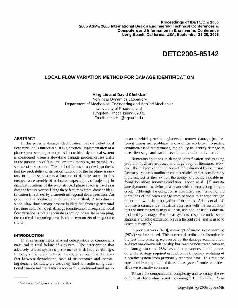
It is obvious that the two Poincare sections were quite simi-lar, and it is hard to describe difference between them. However,if we take a closer look at one particular cell labelled 12 (seeFig. 2), the difference is clear and can be described by the esti-mated first moments.

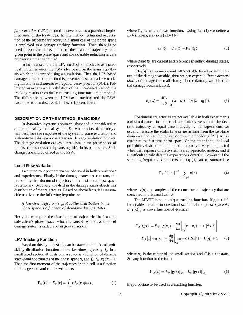
The simulations were repeated 8 times using different initialconditions with both damage states, and the estimated first mo-ments were plotted in Fig. 3. From this plot, we can state thattheobserved difference between two Poincare sections is caused by

−0.8 −0.6 −0.4 −0.2 0−0.5

−0.45

−0.4

−0.35

−0.3

−0.25

−0.2

−0.15

−0.1

−0.05

x

dx

/dt

−0.8 −0.6 −0.4 −0.2 0−0.5

−0.45

−0.4

−0.35

−0.3

−0.25

−0.2

−0.15

−0.1

−0.05

x

dx

/dt

a b

Figure 2. a. Poincare section with c = 0.4; b. Poincare section with

c = 0.41

−0.58 −0.56 −0.54 −0.52 −0.5 −0.48

−0.26

−0.25

−0.24

−0.23

−0.22

−0.21

−0.2

−0.19

Figure 3. Black dots represent the estimated first moments with c= 0.4,

and stars represent the estimated first moments with c = 0.41 using

different initial conditions

change in the damage state instead of change in the initial con-ditions. So these estimated first moments provide valuable infor-mation for identification of the change in damage state. However,because the first moments are estimated using only limited num-ber of about 1700 points, there exists some local fluctuations inthe estimates, and tests based on the LFVTF of a single cell maynot be robust. Although signal-to-noise ratio can be increased ifmore data is used for estimation, it is not possible to collect suchlarge amount of data in an experimental context.

Smooth Orthogonal DecompositionAlthough low signal-to-noise ratio may prevents us from

identifying damage using estimated first moments directly,suchnoisy information can still be handled. In previous study, theSOD [6, 11] based data analysis method has been proven to be

3 Copyright c© 2005 by ASME

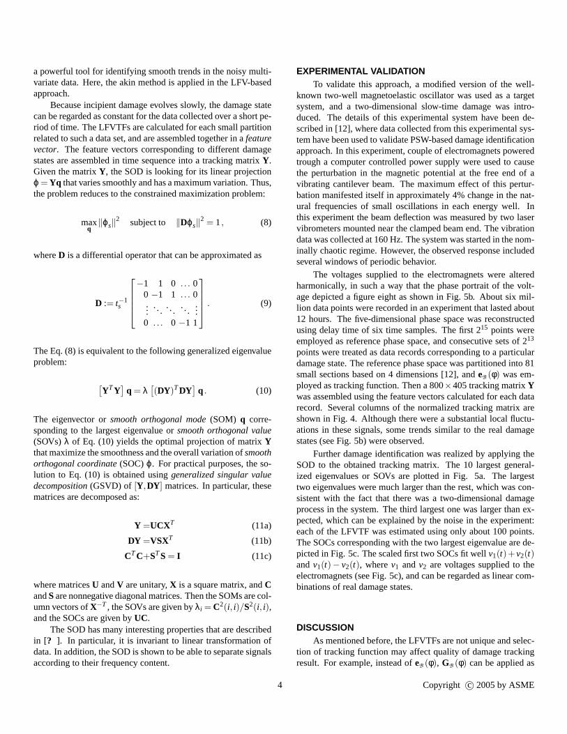
a powerful tool for identifying smooth trends in the noisy multi-variate data. Here, the akin method is applied in the LFV-basedapproach.

Because incipient damage evolves slowly, the damage statecan be regarded as constant for the data collected over a short pe-riod of time. The LFVTFs are calculated for each small partitionrelated to such a data set, and are assembled together in afeaturevector. The feature vectors corresponding to different damagestates are assembled in time sequence into a tracking matrixY.Given the matrixY, the SOD is looking for its linear projectionϕ = Yq that varies smoothly and has a maximum variation. Thus,the problem reduces to the constrained maximization problem:

maxq

‖ϕs‖2 subject to ‖Dϕs‖

2 = 1, (8)

whereD is a differential operator that can be approximated as

D := t−1s

−1 1 0 . . . 00 −1 1 . . . 0...

......

.. ....

0 . . . 0 −1 1

. (9)

The Eq. (8) is equivalent to the following generalized eigenvalueproblem:

[

YTY]

q = λ[

(DY)TDY]

q . (10)

The eigenvector orsmooth orthogonal mode(SOM) q corre-sponding to the largest eigenvalue orsmooth orthogonal value(SOVs)λ of Eq. (10) yields the optimal projection of matrixYthat maximize the smoothness and the overall variation ofsmoothorthogonal coordinate(SOC)ϕ. For practical purposes, the so-lution to Eq. (10) is obtained usinggeneralized singular valuedecomposition(GSVD) of [Y,DY] matrices. In particular, thesematrices are decomposed as:

Y =UCXT (11a)

DY =VSXT (11b)

CTC+STS = I (11c)

where matricesU andV are unitary,X is a square matrix, andCandS are nonnegative diagonal matrices. Then the SOMs are col-umn vectors ofX−T , the SOVs are given byλi = C2(i, i)/S2(i, i),and the SOCs are given byUC.

The SOD has many interesting properties that are describedin [? ]. In particular, it is invariant to linear transformation ofdata. In addition, the SOD is shown to be able to separate signalsaccording to their frequency content.

EXPERIMENTAL VALIDATIONTo validate this approach, a modified version of the well-

known two-well magnetoelastic oscillator was used as a targetsystem, and a two-dimensional slow-time damage was intro-duced. The details of this experimental system have been de-scribed in [12], where data collected from this experimental sys-tem have been used to validate PSW-based damage identificationapproach. In this experiment, couple of electromagnets poweredtrough a computer controlled power supply were used to causethe perturbation in the magnetic potential at the free end ofavibrating cantilever beam. The maximum effect of this pertur-bation manifested itself in approximately 4% change in the nat-ural frequencies of small oscillations in each energy well.Inthis experiment the beam deflection was measured by two laservibrometers mounted near the clamped beam end. The vibrationdata was collected at 160 Hz. The system was started in the nom-inally chaotic regime. However, the observed response includedseveral windows of periodic behavior.

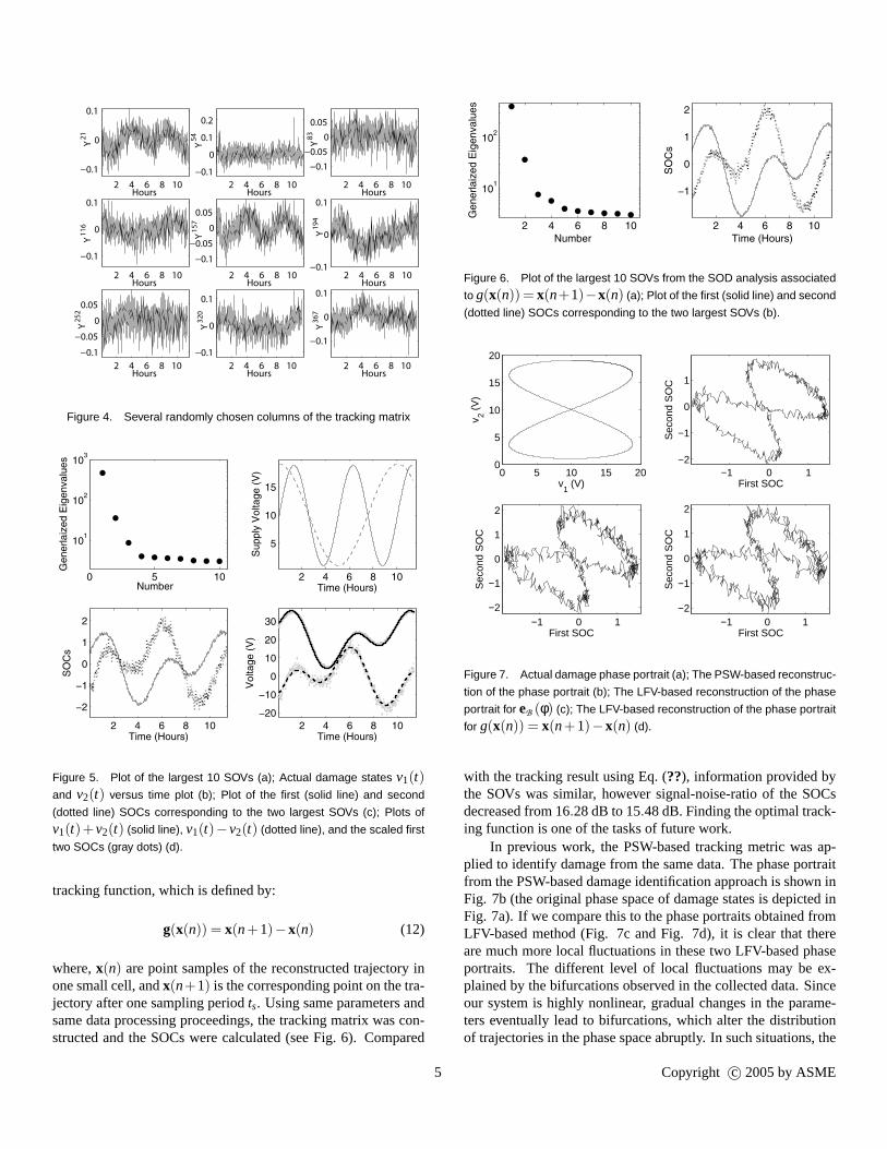
The voltages supplied to the electromagnets were alteredharmonically, in such a way that the phase portrait of the volt-age depicted a figure eight as shown in Fig. 5b. About six mil-lion data points were recorded in an experiment that lasted about12 hours. The five-dimensional phase space was reconstructedusing delay time of six time samples. The first 215 points wereemployed as reference phase space, and consecutive sets of 213

points were treated as data records corresponding to a particulardamage state. The reference phase space was partitioned into 81small sections based on 4 dimensions [12], andeB (φ) was em-ployed as tracking function. Then a 800×405 tracking matrixYwas assembled using the feature vectors calculated for eachdatarecord. Several columns of the normalized tracking matrix areshown in Fig. 4. Although there were a substantial local fluctu-ations in these signals, some trends similar to the real damagestates (see Fig. 5b) were observed.

Further damage identification was realized by applying theSOD to the obtained tracking matrix. The 10 largest general-ized eigenvalues or SOVs are plotted in Fig. 5a. The largesttwo eigenvalues were much larger than the rest, which was con-sistent with the fact that there was a two-dimensional damageprocess in the system. The third largest one was larger than ex-pected, which can be explained by the noise in the experiment:each of the LFVTF was estimated using only about 100 points.The SOCs corresponding with the two largest eigenvalue are de-picted in Fig. 5c. The scaled first two SOCs fit wellv1(t)+v2(t)andv1(t)− v2(t), wherev1 andv2 are voltages supplied to theelectromagnets (see Fig. 5c), and can be regarded as linear com-binations of real damage states.

DISCUSSIONAs mentioned before, the LFVTFs are not unique and selec-

tion of tracking function may affect quality of damage trackingresult. For example, instead ofeB (φ), GB (φ) can be applied as

4 Copyright c© 2005 by ASME

2 4 6 8 10

−0.1

0

0.1

Hours

Y21

2 4 6 8 10

−0.1

0

0.1

0.2

HoursY54

2 4 6 8 10

−0.1

−0.05

0

0.05

Hours

Y83

2 4 6 8 10

−0.1

0

0.1

Hours

Y116

2 4 6 8 10

−0.1

−0.05

0

0.05

Hours

Y157

2 4 6 8 10−0.1

0

0.1

Hours

Y194

2 4 6 8 10

−0.1

−0.05

0

0.05

Hours

Y252

2 4 6 8 10

−0.1

0

0.1

Hours

Y320

2 4 6 8 10

−0.1

0

0.1

Hours

Y367

Figure 4. Several randomly chosen columns of the tracking matrix

0 5 10

101

102

103

Number

Ge

ne

rla

ized

Eig

enva

lue

s

2 4 6 8 10

5

10

15

Time (Hours)

Su

pp

ly V

olta

ge

(V

)

2 4 6 8 10

−2

−1

0

1

2

Time (Hours)

SO

Cs

2 4 6 8 10

−20

−10

0

10

20

30

Time (Hours)

Vo

lta

ge

(V

)

Figure 5. Plot of the largest 10 SOVs (a); Actual damage states v1(t)and v2(t) versus time plot (b); Plot of the first (solid line) and second

(dotted line) SOCs corresponding to the two largest SOVs (c); Plots of

v1(t)+v2(t) (solid line), v1(t)−v2(t) (dotted line), and the scaled first

two SOCs (gray dots) (d).

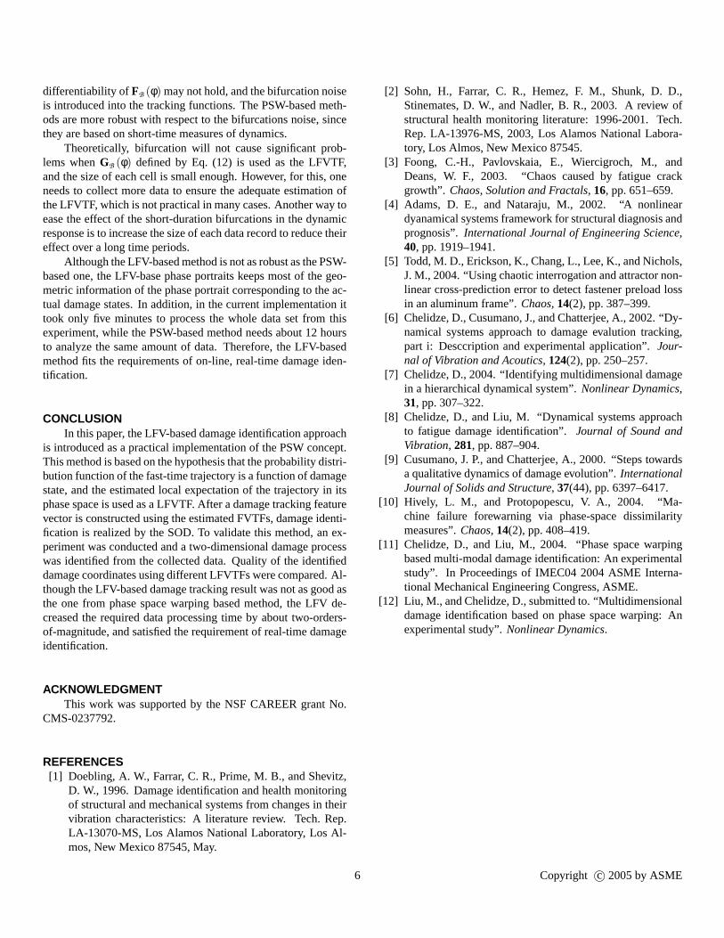
tracking function, which is defined by:

g(x(n)) = x(n+1)−x(n) (12)

where,x(n) are point samples of the reconstructed trajectory inone small cell, andx(n+1) is the corresponding point on the tra-jectory after one sampling periodts. Using same parameters andsame data processing proceedings, the tracking matrix was con-structed and the SOCs were calculated (see Fig. 6). Compared

2 4 6 8 10

101

102

Ge

nerla

ize

d E

ige

nva

lue

s

2 4 6 8 10

−1

0

1

2

SO

Cs

Number Time (Hours)

Figure 6. Plot of the largest 10 SOVs from the SOD analysis associated

to g(x(n)) = x(n+1)−x(n) (a); Plot of the first (solid line) and second

(dotted line) SOCs corresponding to the two largest SOVs (b).

0 5 10 15 200

5

10

15

20

v1 (V)

v 2 (V

)−1 0 1

−2

−1

0

1

First SOC

Sec

ond

SO

C

−1 0 1−2

−1

0

1

2

First SOC

Sec

ond

SO

C

−1 0 1−2

−1

0

1

2

First SOC

Sec

ond

SO

CFigure 7. Actual damage phase portrait (a); The PSW-based reconstruc-

tion of the phase portrait (b); The LFV-based reconstruction of the phase

portrait for eB (φ) (c); The LFV-based reconstruction of the phase portrait

for g(x(n)) = x(n+1)−x(n) (d).

with the tracking result using Eq. (??), information provided bythe SOVs was similar, however signal-noise-ratio of the SOCsdecreased from 16.28 dB to 15.48 dB. Finding the optimal track-ing function is one of the tasks of future work.

In previous work, the PSW-based tracking metric was ap-plied to identify damage from the same data. The phase portraitfrom the PSW-based damage identification approach is shown inFig. 7b (the original phase space of damage states is depicted inFig. 7a). If we compare this to the phase portraits obtained fromLFV-based method (Fig. 7c and Fig. 7d), it is clear that thereare much more local fluctuations in these two LFV-based phaseportraits. The different level of local fluctuations may be ex-plained by the bifurcations observed in the collected data.Sinceour system is highly nonlinear, gradual changes in the parame-ters eventually lead to bifurcations, which alter the distributionof trajectories in the phase space abruptly. In such situations, the

5 Copyright c© 2005 by ASME

differentiability ofFB (φ) may not hold, and the bifurcation noiseis introduced into the tracking functions. The PSW-based meth-ods are more robust with respect to the bifurcations noise, sincethey are based on short-time measures of dynamics.

Theoretically, bifurcation will not cause significant prob-lems whenGB (φ) defined by Eq. (12) is used as the LFVTF,and the size of each cell is small enough. However, for this, oneneeds to collect more data to ensure the adequate estimationofthe LFVTF, which is not practical in many cases. Another way toease the effect of the short-duration bifurcations in the dynamicresponse is to increase the size of each data record to reducetheireffect over a long time periods.

Although the LFV-based method is not as robust as the PSW-based one, the LFV-base phase portraits keeps most of the geo-metric information of the phase portrait corresponding to the ac-tual damage states. In addition, in the current implementation ittook only five minutes to process the whole data set from thisexperiment, while the PSW-based method needs about 12 hoursto analyze the same amount of data. Therefore, the LFV-basedmethod fits the requirements of on-line, real-time damage iden-tification.

CONCLUSIONIn this paper, the LFV-based damage identification approach

is introduced as a practical implementation of the PSW concept.This method is based on the hypothesis that the probability distri-bution function of the fast-time trajectory is a function ofdamagestate, and the estimated local expectation of the trajectory in itsphase space is used as a LFVTF. After a damage tracking featurevector is constructed using the estimated FVTFs, damage identi-fication is realized by the SOD. To validate this method, an ex-periment was conducted and a two-dimensional damage processwas identified from the collected data. Quality of the identifieddamage coordinates using different LFVTFs were compared. Al-though the LFV-based damage tracking result was not as good asthe one from phase space warping based method, the LFV de-creased the required data processing time by about two-orders-of-magnitude, and satisfied the requirement of real-time damageidentification.

ACKNOWLEDGMENTThis work was supported by the NSF CAREER grant No.

CMS-0237792.

REFERENCES[1] Doebling, A. W., Farrar, C. R., Prime, M. B., and Shevitz,

D. W., 1996. Damage identification and health monitoringof structural and mechanical systems from changes in theirvibration characteristics: A literature review. Tech. Rep.LA-13070-MS, Los Alamos National Laboratory, Los Al-mos, New Mexico 87545, May.

[2] Sohn, H., Farrar, C. R., Hemez, F. M., Shunk, D. D.,Stinemates, D. W., and Nadler, B. R., 2003. A review ofstructural health monitoring literature: 1996-2001. Tech.Rep. LA-13976-MS, 2003, Los Alamos National Labora-tory, Los Almos, New Mexico 87545.

[3] Foong, C.-H., Pavlovskaia, E., Wiercigroch, M., andDeans, W. F., 2003. “Chaos caused by fatigue crackgrowth”. Chaos, Solution and Fractals,16, pp. 651–659.

[4] Adams, D. E., and Nataraju, M., 2002. “A nonlineardyanamical systems framework for structural diagnosis andprognosis”. International Journal of Engineering Science,40, pp. 1919–1941.

[5] Todd, M. D., Erickson, K., Chang, L., Lee, K., and Nichols,J. M., 2004. “Using chaotic interrogation and attractor non-linear cross-prediction error to detect fastener preload lossin an aluminum frame”.Chaos,14(2), pp. 387–399.

[6] Chelidze, D., Cusumano, J., and Chatterjee, A., 2002. “Dy-namical systems approach to damage evalution tracking,part i: Desccription and experimental application”.Jour-nal of Vibration and Acoutics,124(2), pp. 250–257.

[7] Chelidze, D., 2004. “Identifying multidimensional damagein a hierarchical dynamical system”.Nonlinear Dynamics,31, pp. 307–322.

[8] Chelidze, D., and Liu, M. “Dynamical systems approachto fatigue damage identification”.Journal of Sound andVibration,281, pp. 887–904.

[9] Cusumano, J. P., and Chatterjee, A., 2000. “Steps towardsa qualitative dynamics of damage evolution”.InternationalJournal of Solids and Structure,37(44), pp. 6397–6417.

[10] Hively, L. M., and Protopopescu, V. A., 2004. “Ma-chine failure forewarning via phase-space dissimilaritymeasures”.Chaos,14(2), pp. 408–419.

[11] Chelidze, D., and Liu, M., 2004. “Phase space warpingbased multi-modal damage identification: An experimentalstudy”. In Proceedings of IMEC04 2004 ASME Interna-tional Mechanical Engineering Congress, ASME.

[12] Liu, M., and Chelidze, D., submitted to. “Multidimensionaldamage identification based on phase space warping: Anexperimental study”.Nonlinear Dynamics.

6 Copyright c© 2005 by ASME