Procedures for Developing Allowable Properties for a Single Species Under ASTM D1990 and Computer Programs Useful for the Calculations James W. Evans David E. Kretschmann Victoria L. Herian David W. Green

United States Department of Agriculture Forest Service Forest Products Laboratory General Technical Report FPL−GTR−126

Abstract ASTM D1990, “Establishing Allowable Properties for Visually Graded Dimension Lumber from In-Grade Tests of Full-Size Specimens,” is the consensus standard used to make submissions of allowable properties for many U.S., Canadian, and foreign species to the Board of Review of the American Lumber Standards Committee. Recently, it has become apparent how difficult it is to perform the calcula-tions for such a submission. Some calculations are clearly specified in the standard; in some cases the standard merely indicates a need to make an adjustment but does not specify how to do so. This report discusses in detail how to develop allowable properties under the standard in a manner that is consistent with current practice. Many calculations in the standard are difficult and errors are easily made, particularly when using a spreadsheet; this report introduces a set of computer programs that perform some of the difficult calcu-lations, thereby reducing the potential for errors. These computer programs can be run over the World Wide Web, or Fortran versions of the programs can be downloaded, compiled, and run on a user’s computer.

Keywords: allowable properties, computer program, ASTM D1990, moisture adjustment, strength ratios, In-Grade

April 2001 Evans, James W.; Kretschmann, David E.; Herian, Victoria L.; Green, David W. 2001. Procedures for developing allowable properties for a single species under ASTM D1990 and computer programs useful for the calculations. Gen. Tech. Rep.. FPL-GTR-126. Madison, WI: U.S. Depart-ment of Agriculture, Forest Service, Forest Products Laboratory. 42 p.

A limited number of free copies of this publication are available to the public from the Forest Products Laboratory, One Gifford Pinchot Drive, Madison, WI 53705–2398. Laboratory publications are sent to hundreds of libraries in the United States and elsewhere.

The Forest Products Laboratory is maintained in cooperation with the University of Wisconsin.

The United States Department of Agriculture (USDA) prohibits discrimina-tion in all its programs and activities on the basis of race, color, national origin, sex, religion, age, disability, political beliefs, sexual orientation, or marital or familial status. (Not all prohibited bases apply to all programs.) Persons with disabilities who require alternative means for communication of program information (Braille, large print, audiotape, etc.) should contact the USDA’s TARGET Center at (202) 720–2600 (voice and TDD). To file a complaint of discrimination, write USDA, Director, Office of Civil Rights, Room 326-W, Whitten Building, 1400 Independence Avenue, SW, Wash-ington, DC 20250–9410, or call (202) 720–5964 (voice and TDD). USDA is an equal opportunity provider and employer.

Metric equivalents

Inch–pound unit Conversion factor Metric unit

inch (in.) 25.4 mm

pound (lb) 4.4482 N

lb/in2 6.8948 × 103 Pa

temperature in °F (TF) (TF – 32)/1.8 temperature in °C

board foot 2.3597 × 10–3 m3

Nominal lumber size (in.)

Standard lumber size (mm)

2 by 4 38 by 89

2 by 6 38 by 140

2 by 8 38 by 184

2 by 10 38 by 235

2 by 12 38 by 286

Contents Page

A. Introduction.......................................................................1

B. Background.......................................................................1

B.1 ASTM D1990..............................................................1

B.2 Need for this report .....................................................2

C. Factors affecting the representativeness of the sample .....2

C.1 Grade quality index.....................................................2

C.2 Choosing a sampling matrix........................................3

C.3. Collecting the test data ...............................................4

D. Step by step through D1990 for one species.....................5

D.1 Adjust for loading conditions .....................................5

D.2 Adjust for GQI............................................................7

D.3 Adjust recorded temperature.......................................7

D.4 Adjust moisture content readings................................7

D.5 Adjust strength properties for temperature .................7

D.6 Adjust data to 15% moisture content ..........................9

D.7 Calculate summary statistics.....................................10

D.8 Adjust dimensions of the specimens to 15% moisture content ......................................................10

D.9 Adjust property values to the characteristic size.......11

D.10 Establish the characteristic values ..........................11

D.11 Conduct the section 9.3 and section 12.6 data checks.......................................................................12

D.12 Estimate characteristic values for untested properties...........................................................12

D.13 Develop allowable properties from the final characteristic values for a full sampling matrix ...............13

D.14 Values for other sizes and grades and handling a less than full sampling matrix ........................14

Page

E. Computer programs useful in developing allowable properties............................................................ 15

E.1 Anonymous ftp......................................................... 15

E.2 Grade quality index (strength ratio) program SRATIO ........................................................... 17

E.3 Temperature adjustment program TEMPADJ.......... 18

E.4 Moisture content adjustment program MCADJ ....... 22

E.5 Nonparametric estimation program NONPAR......... 22

E.6 Testing cell data checks of section 9.3 and 12.6 of ASTM D1990 DATACHECK ................................... 28

E.7 ALLFROMR—Program to calculate MOR, UTS, and UCS design values from MOR characteristic values........................................................ 29

E.8 EDESIGN—Program to calculate MOE design values from MOE characteristic values .......................... 29

F. Discussion and Summary ............................................... 39

G. References...................................................................... 39

H. Appendix 1—New temperature adjustment procedure ............................................................................ 41

I. Appendix 2—Strength ratio calculations ........................ 41

I.1. Narrow face knots or spike knots ............................. 41

I.2. Center of wide face knots......................................... 41

I.3. Edge of wide face knots ........................................... 42

I.4. Combination knots ................................................... 42

I.5. Distorted grain.......................................................... 42

I.6. Slope of grain ........................................................... 42

I.7. Clear wood or no failure........................................... 42

Procedures for Developing Allowable Properties for a Single Species Under ASTM D1990 and Computer Programs Useful for the Calculations James W. Evans, Supervisory Mathematical Statistician David E. Kretschmann, Research General Engineer Victoria L. Herian, Statistician David W. Green, Supervisory Research General Engineer Forest Products Laboratory, Madison, Wisconsin

A. Introduction The purpose of this report is to explain and simplify the process of developing allowable properties for visually graded dimension lumber under ASTM D1990 (ASTM 1998). This report provides a brief background of ASTM D1990 followed by a discussion of issues to consider when obtaining a representative sample. Then a step-by-step “walk through” of the standard for a single species is described. This walk through follows the pattern of the most recent submissions to the Board of Review (BOR) of the American Lumber Standard Committee (ALSC) in that it assumes the specimens were tested in bending only. The standard does allow testing in tension and compression, but for economic reasons, recent submissions have used only bending tests. Finally, a series of computer programs (available on the internet) that perform many of the calculations needed in a submission are outlined. This report is not intended to re-place ASTM D1990 or to document the reasoning behind the standard. It assumes that anyone developing allowable prop-erties has a copy of and is following the standard.

B. Background B.1 ASTM D1990 ASTM D1990, “Establishing Allowable Properties for Visu-ally-Graded Dimension Lumber from In-Grade Tests of Full-Size Specimens,” is a by-product of the U.S. In-Grade Test-ing Program begun in 1977 by the USDA Forest Service, Forest Products Laboratory, in cooperation with the major rules-writing grading agencies in the United States. The objectives of the program were to evaluate the mechanical properties of 2-in. dimension lumber sold in the United States and to develop analytical models to predict the

performance of light-frame structures constructed using this lumber. Green and Evans (1988e) discuss in detail some of the decisions required in carrying out such a program.

The result of the program was the testing of more than 70,000 specimens, totalling approximately 1,000,000 board feet of lumber, in bending, tension parallel to grain, and compression parallel to grain. This 10-year, $7 million dollar effort was one of the largest single research efforts ever undertaken in forest products research. To coordinate this effort, the In-Grade Program Technical Committee was formed. Initially composed of technical representatives of the Forest Products Laboratory, West Coast Lumber Inspec-tion Bureau, Western Wood Products Association, and Southern Pine Inspection Bureau, the committee expanded over time to include representatives of the Northern Hard-wood and Pine Manufacturers Association, Northeastern Lumber Manufacturers’ Association, Canadian Wood Coun-cil, University of British Columbia, Forintek Canada Corp., and Fletcher Challenge Canada. Representatives of the American Forest and Paper Association were often present at meetings. This combined program is called the North American In-Grade Testing Program.

The In-Grade Program Technical Committee was faced with the task of taking physical and mechanical property informa-tion on 33 species or species groups and using it to establish allowable design properties. This required numerous sup-porting research studies and the gathering of current research information to make a series of decisions on how to adjust raw data taken in the field, under a variety of temperature and humidity conditions, to common conditions. Adjust-ments for moisture content, temperature, and species differ-ences in moisture meter readings are just three of many adjustments that are part of the process of converting the

2

data to allowable properties. Many of these decisions and the technical basis for them are found in Green and others (1989). Performing these adjustments resulted in a series of publications of adjusted property values (Green and Evans 1988a–d, Evans and Green 1988a–d).

Implementation of In-Grade procedures resulted in modifica-tion of an existing ASTM standard and development of two new ASTM standards. ASTM D2915 was modified to incor-porate more information on sampling procedures, to allow for both parametric and nonparametric calculations, and to expand the significance levels allowed in calculations. ASTM D4761 was developed to provide methods for testing lumber under field conditions. ASTM D1990 was developed to provide procedures for calculating allowable properties from In-Grade data. ASTM D1990 does not follow exactly all the decisions made by the In-Grade Program Technical Committee, but it does incorporate most of them. ASTM D1990 also leaves out information on how to make certain adjustments that are often part of the process of calculating allowable properties. This report draws together the informa-tion needed to make this calculation.

B.2 Need for this report Developers of any ASTM standard find it difficult, if not impossible, to anticipate all possible uses of its procedures. This is especially true of new standards. Having been estab-lished in 1991, ASTM D1990 is a relatively new standard. Under the provisions of Voluntary Product Standard PS20 (Green and Hernandez 1998), the BOR of the ALSC ap-proves assignments of allowable properties using ASTM standards and other technically sound criteria. This means that the BOR must make technically sound interpretations of ASTM D1990 provisions for those situations where the standard is vague. Since the original submissions of allow-able properties to the BOR using ASTM D1990, several submissions have been made for foreign species (Green and Shelley 1994). In most cases, the calculations were per-formed by individuals who did not participate in the original submissions or the In-Grade Program, and the difficulty in making the calculations became apparent. Some calculations are clearly specified in the standard. However, in some cases the standard merely indicates a need to make an adjustment but does not specify how to do so. In addition, several years have elapsed since the original submissions were made under ASTM D1990. Part of any system of developing allowable properties should be consistency in calculations across species. That becomes more difficult as more people become involved in performing the calculations. Therefore, some record of what has been done in the past is also impor-tant. Finally, many of the calculations in the standard are difficult, and mistakes are easily made, particularly when trying to integrate the calculations in a spreadsheet, as most recent submissions have done. The development of computer programs to perform some of the calculations can simplify the process and eliminate some potential errors.

C. Factors affecting the representativeness of the sample ASTM D1990 defines “In-Grade” as samples collected from lumber grades as commercially produced. Section 1.2 of ASTM D1990 states “A basic assumption of the procedures used in this practice is that the samples selected and tested are representative of the entire global population being evaluated.” In the In-Grade Testing Program, great care was taken to ensure that this was the case (see Jones (1989) for a detailed discussion). First, the lumber was sampled to ensure geographic representativeness. For major species, the geo-graphic area over which the species grew was divided into regions judged to be homogeneous. Historical clear wood property data and information on variation in climatic factors known to effect tree growth were used to make this judg-ment. Specimens were sampled by region in proportion to production, with a total sample size of 360 to 400 samples per size–grade–test mode combination. At a mill, samples were selected from randomly chosen bunks of lumber, with no more than 20 specimens taken at a mill for a given size–grade cell combination. The size–grade combinations were chosen to be representative of most lumber production. For major species, two grades (Select Structural and No. 2) and three sizes (nominal 2 by 4, 2 by 8, and 2 by 10 in., hereafter referred to as 2×4, 2×8, and 2×10, respectively) were sam-pled. ASTM D1990 calls the combination of grades and sizes tested for a given species and test mode the “sampling matrix.” Finally, the lumber was chosen to be representative of lumber sold within a specific grade. The “grade quality index” (GQI) provides a numerical assessment of the charac-teristics found in the sampled specimens that are considered to be related to strength and that are limited as part of the grade description. GQIs were calculated for each piece of lumber tested in the In-Grade Program.

C.1 Grade quality index An “In-Grade” sample is assumed to be representative of commercial lumber production. Such samples are thus in-tended to represent the full range of strength and modulus of elasticity values normally found in the grade. ASTM D1990 (paragraph 8.2) states that if the observed GQI from the sample varies from the assumed GQI for the grade by more than 5%, the sample and the GQI shall be reevaluated for appropriateness. In practice, the primary concern has been for samples with a GQI more than 5% above the assumed GQI for the grade, because such samples would be expected to have properties that are greater than those typical for the grade.

The GQI based on strength ratios and used in the In-Grade Program has been also used in all subsequent submissions to the BOR. The type of failure of a specimen was recorded using the appropriate failure code found in table X1.1 of the

3

appendix in ASTM D4761. Strength ratios, as defined in ASTM D245, were calculated according to the formulas in ASTM D245, with the exception that narrow face knots were converted to equivalent edge of wide face knots. After excluding specimens that failed in clear wood, and therefore had strength ratios of 100%, and specimens whose failure code did not allow calculation of a strength ratio, such as local slope of grain, the 5th percentile of the remaining strength ratios was calculated and compared with the strength ratio associated with the grade. If it was within 5% of the GQI for the grade based on the total GQI range (that is, with the strength ratio range of 0 to 100, a No. 2 grade with assumed strength ratio of 45 should be within 40 to 50), the sample was said to be representative of the grade.

The vagueness of the discussion of GQI in the standard raises several issues:

1. GQI has a very broad definition. ASTM D1990 allows something other than strength ratios to be used. No one has used anything else in a submission to date. It would clearly present a challenge if someone proposed some other method of determining grade quality index.

2. The standard does not specifically state what to do if you fail a GQI test. In the In-Grade Program, the GQI for every size–grade cell of every major species was within the 5% GQI limit. This has not been the case with many foreign species. For foreign species, four methods of adjustment have been proposed and three methods have been used in submissions. To illustrate the four methods, assume that for a sample of 2×4 No. 2 structural dimension lumber, the 5th-percentile strength ratio was 51%, which exceeds by more than 5% the as-sumed 45% strength ratio of the grade and brings into question the representativeness of the sample for the grade. To this point, submissions failing the GQI test have made an adjustment to the mechanical properties that is designed to provide the mechanical properties that a representative sample would have produced. The four adjustments that have been identified are all calcu-lated numbers that by which property values in the cell would be multiplied. Methods 1 and 2 are ratio adjust-ments, the difference being whether the data are ad-justed to the assumed mean of the size–grade cell or the upper bound of what might be allowable. So in method 1, the properties are multiplied by 45/51, and in method 2 by 50/51. The other two methods calculate the per-centage that the sample GQI exceeds the assumed GQI. Again the assumed GQI can be either the mean or upper bound. So in method 3 the properties are multiplied by 1 – [(51–45)/45], and in method 4 by 1 – [(51–50)/ 50]. All but method 4 have been used in submissions. Method 1 is probably the best and is the method that all recent submissions have used.

3. There is also no discussion of how to apply the GQI data check for species that are to be grouped under the standard. Should every size–grade cell of every species tested have to meet the GQI test? In the process of grouping data, all the species are combined. Should the combined data have to meet the GQI test? Finally, as part of grouping, a controlling subgroup of species that are indistinguishable from the weakest species is created for each grade. Should the controlling subgroup have to pass the GQI test? Clearly having every species pass the GQI test in every size–grade cell tested is the most con-servative approach and probably the most defensible. However, sample sizes for species to be grouped were often small (approximately 60 per size–grade cell in-stead of 360). With smaller sample sizes, a species will more likely fail the GQI test because of the greater variability of a 5th-percentile estimate.

C.2 Choosing a sampling matrix Another representativeness issue is how many size–grade cells are to be sampled. The standard, in section 7, recog-nizes three conditions:

1. Condition 1 is when only one size (such as 2×4) of lumber is to be sampled. In this situation, it is necessary to sample “two grades representative of the range of grade quality.” In practice, this means sampling Select Structural (SS) and No. 2 grade material because the grade model of section X8, which is used to create val-ues for untested grades, is anchored by the SS and No. 2 values. This case allows the calculation of allowable properties for all grades of one size.

2. Condition 2 is when only one grade (such as No. 2) is to be sampled. In this situation, three widths of material must be tested where the maximum difference in any two widths is 4 in. In the In-Grade Program, major spe-cies were tested as 2×4, 2×8, and 2×10, and minor spe-cies as 2×4, 2×6, and 2×8. Recent foreign submissions have been for 2×4, 2×6, and 2×8. This case allows the calculation of allowable properties for all sizes of one grade.

3. Condition 3 is called a full matrix. In this case, three sizes of each of two grades are tested. The standard does place some limits on the choice of sizes and grades. The grade model in the standard appendix uses SS and No. 2 grades, and the sizes chosen must be such that “the maximum difference in width between two adjacent widths shall be 4 in. (10 cm).” This condition allows development of allowable properties for the full range of sizes and grades. Additional grades and sizes can also be tested.

At least two other conditions (called conditions 4 and 5 for purposes of discussion) could occur:

4

4. Condition 4 is when two grades, such as SS and No. 2, are sampled for each of two sizes, usually 2×4 and 2×6. Clearly, the standard would allow this to be considered as two separate cases of condition 1 in calculating al-lowable properties for all grades of the two sizes. What the standard does not say is whether the calculations for each size should be done independently of each other or to use some of the size smoothing models of the full ma-trix approach. This condition has arisen once, and the decision reached by the agency submitting the species and approved by the BOR was to treat this partial matrix as a full matrix in the calculations, so as to preserve size relationships. When completed, however, only values for the two sizes (and all grades) were claimed.

5. Condition 5 is when one size–grade cell is tested, such as 2×4 No. 2. Section 4.2 of the standard states that this condition should be covered in ASTM D2915. This op-tion has not been utilized since ASTM D1990 was es-tablished. There are two notable differences between the ASTM D1990 and ASTM D2915 approaches. First, ASTM D2915 does not give guidelines as to what sam-ple size might constitute a “representative” sample, whereas ASTM D1990 provides these guidelines. Sec-ond, ASTM D245 is referenced in D2915 for moisture content adjustments (Green and Evans 2000b). While these adjustments might be appropriate for tests involv-ing clear wood, they are not appropriate for adjusting test data for dimension lumber. ASTM D1990 guide-lines should be followed for these two items if one con-templates submissions of a single size–grade cell of In-Grade data to the BOR.

C.3. Collecting the test data How the test data are determined and recorded has a direct impact on the ability of the BOR to judge its representative-ness. Three key aspects of the testing need to be considered: equipment calibration, information to be collected, and testing procedures. What is recorded depends on the test modes (bending, tension, and/or compression) to be evalu-ated.

C.3.1 Equipment calibration The calibration of equipment is critical for accurate test results. Guidance for calibrations of testing machines is given in ASTM D4761 and an article in the “In-Grade Test-ing of Structural Materials” proceedings (Shelley 1989). The following suggested practices should be considered particu-larly important:

1. Allow enough time for warm-up of the electronics and hydraulics before calibration.

2. Identify and document the method used for calibrating load cells (proof ring or aluminum bars).

3. Make sure that the proper machine correction informa-tion is known for the test equipment used. The machine correction information is meant to compensate for the flexibility in the test frame.

4. Make sure that a calibration procedure is used that will calibrate the test equipment at the beginning of each day and every 4 hours during testing.

5. Finally, the thermometers used to determine the tem-perature at the time of test should be calibrated so that the relationship between their readings and a reference thermometer are known.

C.3.2 Information to be collected For each piece of lumber the following test information should be measured or recorded if possible:

1. Piece no. — An identification number unique to each piece tested

2. Size — Actual size to nearest 1/32 in. (0.03 in.) for width and thickness, both measured at the center of the piece

3. Actual grade — Actual grade as determined by the qual-ity supervisor of a grading agency

4. Moisture content — Preferably determined by ovendry measurements, otherwise using a resistance meter with a two-pin insulated probe inserted to 5/16-in. depth at the center of the piece length (being sure to appropriately apply a species correction factor)

5. Temperature — Ambient and representative lumber surface temperatures for each day (Judgment should be applied here. If temperature remains relatively constant throughout the day, once a day is sufficient. If tempera-ture changes throughout the day, readings should be taken more often.)

6. Rings per inch — Estimate of growth rings per inch for each piece

7. Percent summer wood — Estimate of percentage sum-mer wood when distinct rings are present

8. Pith present — Whether or not the pith is present in the piece

9. Loading rate — The rate at which the material has been loaded (in./min)

10. Load deflection record — A load deflection history of sufficient length to determine the modulus of elasticity from the initial linear portion of the curve. (For stress-graded lumber, data obtained for loads corresponding to a maximum stress in the specimen between 400 and 1,000 lb/in2 will usually be adequate.)

5

11. Max load — Maximum load (lb) for each test

12. Failure code — Description of defect that initiated the failure according to the suggested scheme from table X1.1 of ASTM D4761 (This is perhaps the most criti-cal defect information as this code is used to establish the GQI.)

13. MOE — Edgewise modulus of elasticity

14. MOR — Modulus of rupture.

15. SPGR — Specific gravity based on volume at time of test and preferably ovendry weight

16. Time to failure — For each piece

C3.3 Test procedures The testing procedures are covered in D198 and D4761. Note that D198 and D4761 do not give identical results, but under D1990 either is an acceptable method. Pellerin and Gerhards (1980) showed that testing under D4761 is slightly more conservative than under D198. The test procedures used in the original In-Grade Program are discussed in detail by Shelley (1989). The procedures of particular importance are the following:

1. Make sure that the test span is within the range of 17 to 21 times the depth. 17 to 1 was used in the In-Grade Program.

2. Make sure that the loading rate produces failure in about 1 to 2 min.

3. When establishing MOE value for a test specimen, repeat sufficient times to verify its repeatability. In the In-Grade Program this was usually done three times. The resulting readings were then averaged.

4. For the bending test, place the defects up or down and right or left randomly within the constant moment zone.

5. If shear and compression perpendicular to the grain are required, make sure the numbering scheme employed al-lows any clear wood specimens cut from a piece of lum-ber to be traced back to original piece.

D. Step by step through D1990 for one species After the data are collected and the GQI evaluated, MOE and MOR values must be adjusted to standard conditions and certain summary statistics reported. The standard is vague when discussing the adjustments to be used in several places. For example, section 8.3.1 states “Test samples at 73 ± 5°F (23 ± 3°C). When this is not possible, adjust indi-vidual test data to 73°F (23°C) by an adjustment model demonstrated to be appropriate.” The following section

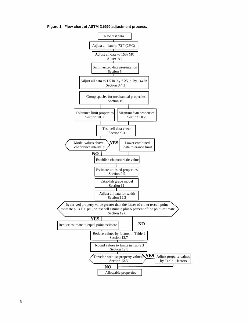
discusses, step by step, how allowable properties for a repre-sentative sample of one species, tested in bending only, are calculated. Included is discussion of how various non-standard conditions have been handled in previous submis-sions to the BOR. This is not to imply that they are the only acceptable way of making adjustments. However, they do offer a way that has been judged acceptable in the past. Also, because some of the adjustments are not simply multiplica-tion of a factor times a strength property, the order of ad-justment can be important. The adjustments are presented in the most logical order. Figure 1 shows the flow chart pub-lished in the standard, which may be helpful in understand-ing the steps of the process.

D.1 Adjust for loading conditions ASTM D1990 refers to ASTM D198 and ASTM D4761 for mechanical test methods. These standards offer a wealth of information on the mechanical test methods that can be used. Missing from these standards is identification of test condi-tions that are consistent with adjustments used in calculating allowable properties. All submissions of allowable proper-ties for MOR to the BOR from the In-Grade Program are based on bending tests that are third-point loaded with a 17-to-1 span-to-depth ratio. The MOE values have deflec-tions measured at the load heads. Generally, they have also been measured at 17 to 1. The standard does not require that third-point loading be done with a 17-to-1 span-to-depth ratio. However, many of the data adjustments (such as mois-ture content) were based on models developed from tests done at 17 to 1 with third-point loading. Their applicability to the test conditions depends upon how different those test conditions are from the assumed conditions.

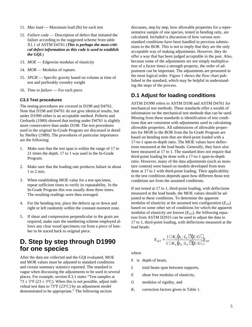
If not tested at 17 to 1, third-point loading, with deflections measured at the load heads, the MOE values should be ad-justed to these conditions. To determine the apparent modulus of elasticity at the assumed test configuration (Eai2) based on some other set of conditions for which the apparent modulus of elasticity are known (Eai1), the following equa-tion from ASTM D2915 can be used to adjust the data to 17 to 1, third-point loading, with deflections measured at the load heads:

( ) ( )( ) ( ) 12

222

2111

21

1aiai E

GELhK

GELhKE

++

=

where

h is depth of beam,

L total beam span between supports,

E shear free modulus of elasticity,

G modulus of rigidity, and

Ki correction factors given in Table 1.

6

Figure 1. Flow chart of ASTM D1990 adjustment process.

Reduce values by factors in Table 2 Section 12.7

Raw test data

Adjust all data to 73 o F (23 o C)

Adjust all data to 15% MC Annex A1

Summarized data presentation Section 5

Adjust all data to 1.5 in. by 7.25 in. by 144 in. Section 8.4.3

Group species for mechanical properties Section 10

Tolerance limit properties Section 10.3

Mean/median properties Section 10.2

Test cell data check Section 9.3

Model values above confidence interval?

Lower combined data tolerance limit

Establish characteristic value

Estimate untested properties Section 9.5

Establish grade model Section 11

Is derived property value greater than the lesser of either test cell point estimate plus 100 psi , or test cell estimate plus 5 percent of the point estimate?

Section 12.6

Round values to limits in Table 3 Section 12.8

Develop wet use property values? Section 12.5

Adjust property values by Table 1 factors

Allowable properties

Adjust all data for width Section 12.2

YES

NO

NO YES

YES

NO

Reduce values by factors in Table 2 Section 12.7

Raw test data

Adjust all data to 73 o F (23 o C)

Adjust all data to 15% MC Annex A1

Summarized data presentation Section 5

Adjust all data to 1.5 in. by 7.25 in. by 144 in. Section 8.4.3

Group species for mechanical properties Section 10

Tolerance limit properties Section 10.3

Mean/median properties Section 10.2

Test cell data check Section 9.3

Model values above confidence interval?

Lower combined data tolerance limit

Establish characteristic value

Estimate untested properties Section 9.5

Establish grade model Section 11

Is derived property value greater than the lesser of either test cell point estimate plus 100 psi , or test cell estimate plus 5 percent of the point estimate?

Section 12.6

Reduce estimate to equal point estimate

Round values to limits in Table 3 Section 12.8

Develop wet use property values? Section 12.5

Adjust property values by Table 1 factors

Allowable properties

Adjust all data for width Section 12.2

NO

YES

7

D.2 Adjust for GQI The second adjustment should be for any cells that fail the GQI test. As previously mentioned, method 1, which uses a ratio of the assumed cell GQI over the actual cell GQI, is probably the best method. In calculating the actual cell GQI, the number produced most likely has a decimal representa-tion, such as 51.246, because the 5th percentile of the GQI values that are not 100% is usually an interpolated value. These values should be rounded up, preferably to the next integer value (52 in this example), although some submis-sions have rounded up in the first decimal (51.3 in this example).

D.3 Adjust recorded temperature The thermometer used to measure temperature is often as-sumed to be accurate. In the In-Grade Program, the ther-mometers used to measure air and wood temperature were actually calibrated. In cases where these same thermometers were used in other submissions, the values were adjusted based on the earlier calibrations.

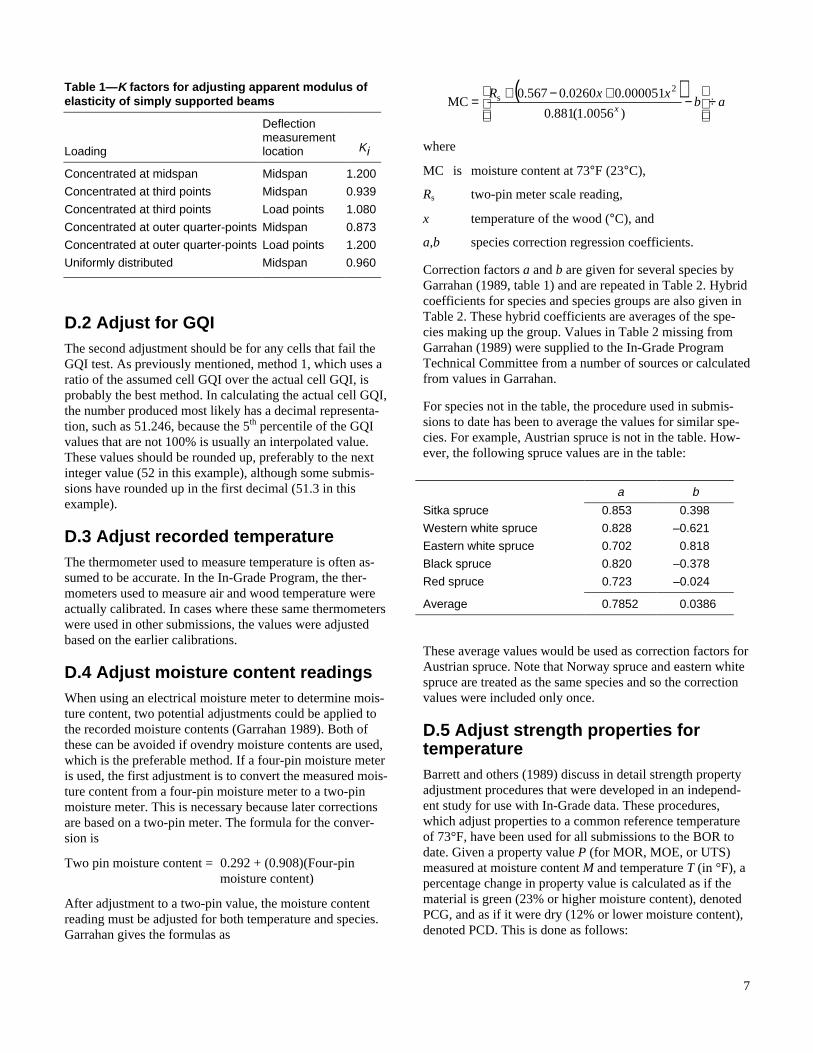
D.4 Adjust moisture content readings When using an electrical moisture meter to determine mois-ture content, two potential adjustments could be applied to the recorded moisture contents (Garrahan 1989). Both of these can be avoided if ovendry moisture contents are used, which is the preferable method. If a four-pin moisture meter is used, the first adjustment is to convert the measured mois-ture content from a four-pin moisture meter to a two-pin moisture meter. This is necessary because later corrections are based on a two-pin meter. The formula for the conver-sion is

Two pin moisture content = 0.292 + (0.908)(Four-pin moisture content)

After adjustment to a two-pin value, the moisture content reading must be adjusted for both temperature and species. Garrahan gives the formulas as

( )ab

xxRx

÷

−+−+=

)0056.1(881.0

000051.00260.0567.0MC

2s

where

MC is moisture content at 73°F (23°C),

Rs two-pin meter scale reading,

x temperature of the wood (°C), and

a,b species correction regression coefficients.

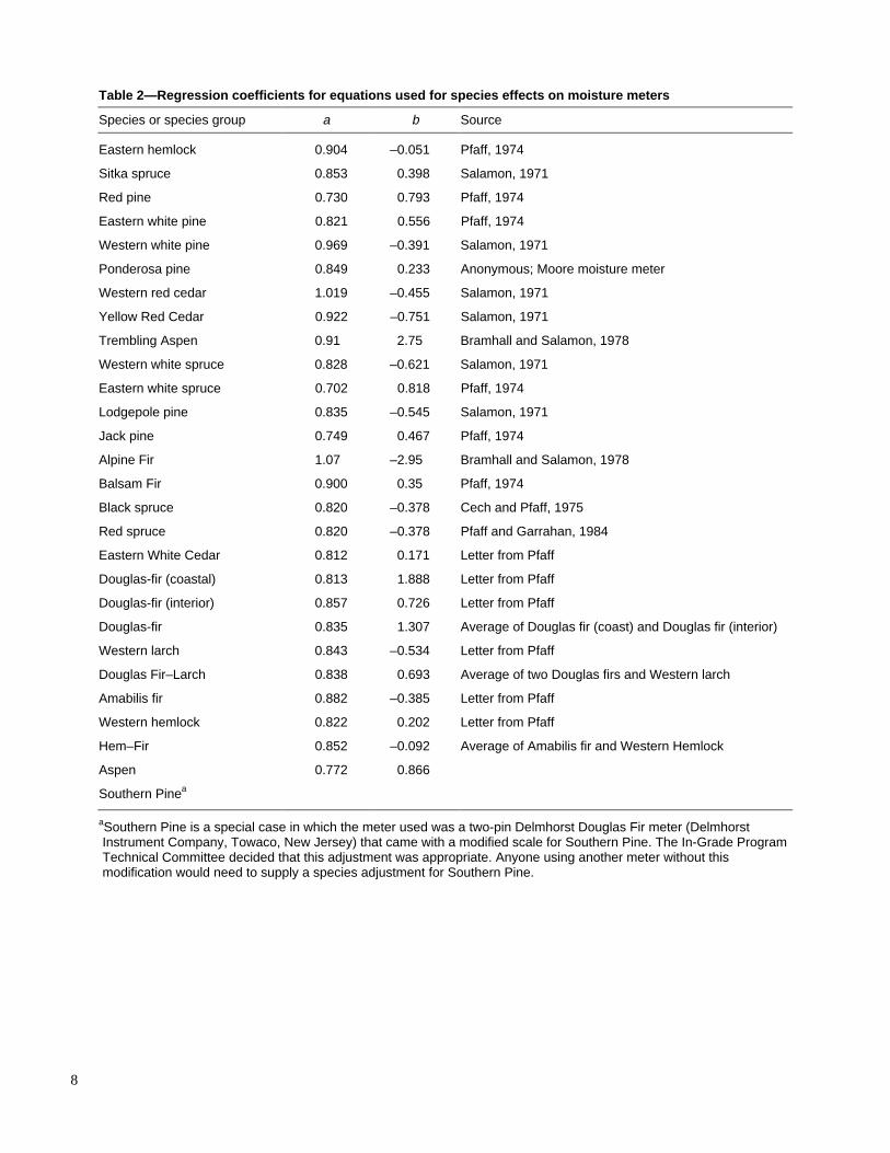
Correction factors a and b are given for several species by Garrahan (1989, table 1) and are repeated in Table 2. Hybrid coefficients for species and species groups are also given in Table 2. These hybrid coefficients are averages of the spe-cies making up the group. Values in Table 2 missing from Garrahan (1989) were supplied to the In-Grade Program Technical Committee from a number of sources or calculated from values in Garrahan.

For species not in the table, the procedure used in submis-sions to date has been to average the values for similar spe-cies. For example, Austrian spruce is not in the table. How-ever, the following spruce values are in the table:

a b

Sitka spruce 0.853 0.398

Western white spruce 0.828 –0.621

Eastern white spruce 0.702 0.818

Black spruce 0.820 –0.378

Red spruce 0.723 –0.024

Average 0.7852 0.0386

These average values would be used as correction factors for Austrian spruce. Note that Norway spruce and eastern white spruce are treated as the same species and so the correction values were included only once.

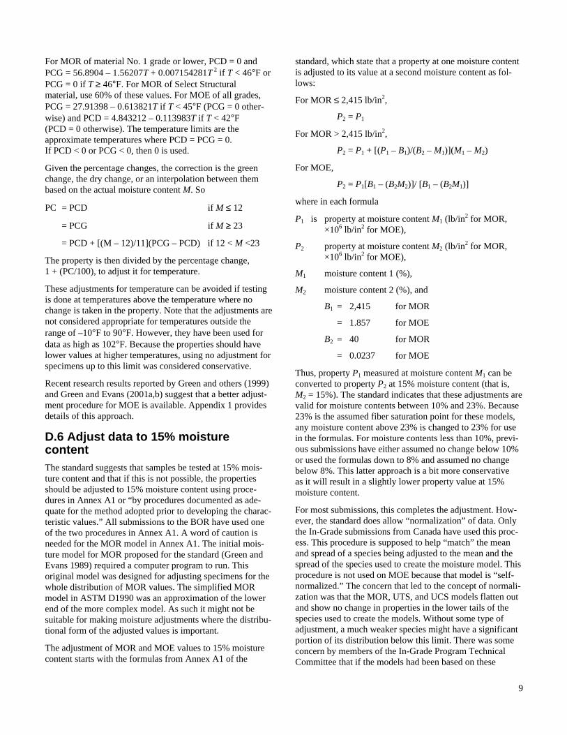
D.5 Adjust strength properties for temperature Barrett and others (1989) discuss in detail strength property adjustment procedures that were developed in an independ-ent study for use with In-Grade data. These procedures, which adjust properties to a common reference temperature of 73°F, have been used for all submissions to the BOR to date. Given a property value P (for MOR, MOE, or UTS) measured at moisture content M and temperature T (in °F), a percentage change in property value is calculated as if the material is green (23% or higher moisture content), denoted PCG, and as if it were dry (12% or lower moisture content), denoted PCD. This is done as follows:

Table 1—K factors for adjusting apparent modulus of elasticity of simply supported beams

Loading

Deflection measurement location Ki

Concentrated at midspan Midspan 1.200

Concentrated at third points Midspan 0.939

Concentrated at third points Load points 1.080

Concentrated at outer quarter-points Midspan 0.873

Concentrated at outer quarter-points Load points 1.200

Uniformly distributed Midspan 0.960

8

Table 2—Regression coefficients for equations used for species effects on moisture meters

Species or species group a b Source

Eastern hemlock 0.904 –0.051 Pfaff, 1974

Sitka spruce 0.853 0.398 Salamon, 1971

Red pine 0.730 0.793 Pfaff, 1974

Eastern white pine 0.821 0.556 Pfaff, 1974

Western white pine 0.969 –0.391 Salamon, 1971

Ponderosa pine 0.849 0.233 Anonymous; Moore moisture meter

Western red cedar 1.019 –0.455 Salamon, 1971

Yellow Red Cedar 0.922 –0.751 Salamon, 1971

Trembling Aspen 0.91 2.75 Bramhall and Salamon, 1978

Western white spruce 0.828 –0.621 Salamon, 1971

Eastern white spruce 0.702 0.818 Pfaff, 1974

Lodgepole pine 0.835 –0.545 Salamon, 1971

Jack pine 0.749 0.467 Pfaff, 1974

Alpine Fir 1.07 –2.95 Bramhall and Salamon, 1978

Balsam Fir 0.900 0.35 Pfaff, 1974

Black spruce 0.820 –0.378 Cech and Pfaff, 1975

Red spruce 0.820 –0.378 Pfaff and Garrahan, 1984

Eastern White Cedar 0.812 0.171 Letter from Pfaff

Douglas-fir (coastal) 0.813 1.888 Letter from Pfaff

Douglas-fir (interior) 0.857 0.726 Letter from Pfaff

Douglas-fir 0.835 1.307 Average of Douglas fir (coast) and Douglas fir (interior)

Western larch 0.843 –0.534 Letter from Pfaff

Douglas Fir–Larch 0.838 0.693 Average of two Douglas firs and Western larch

Amabilis fir 0.882 –0.385 Letter from Pfaff

Western hemlock 0.822 0.202 Letter from Pfaff

Hem–Fir 0.852 –0.092 Average of Amabilis fir and Western Hemlock

Aspen 0.772 0.866

Southern Pinea

aSouthern Pine is a special case in which the meter used was a two-pin Delmhorst Douglas Fir meter (Delmhorst Instrument Company, Towaco, New Jersey) that came with a modified scale for Southern Pine. The In-Grade Program Technical Committee decided that this adjustment was appropriate. Anyone using another meter without this modification would need to supply a species adjustment for Southern Pine.

9

For MOR of material No. 1 grade or lower, PCD = 0 and PCG = 56.8904 – 1.56207T + 0.007154281T 2 if T < 46°F or PCG = 0 if T ≥ 46°F. For MOR of Select Structural material, use 60% of these values. For MOE of all grades, PCG = 27.91398 – 0.613821T if T < 45°F (PCG = 0 other-wise) and PCD = 4.843212 – 0.113983T if T < 42°F (PCD = 0 otherwise). The temperature limits are the approximate temperatures where PCD = PCG = 0. If PCD < 0 or PCG < 0, then 0 is used.

Given the percentage changes, the correction is the green change, the dry change, or an interpolation between them based on the actual moisture content M. So

PC = PCD if M ≤ 12

= PCG if M ≥ 23

= PCD + [(M – 12)/11](PCG – PCD) if 12 < M <23

The property is then divided by the percentage change, 1 + (PC/100), to adjust it for temperature.

These adjustments for temperature can be avoided if testing is done at temperatures above the temperature where no change is taken in the property. Note that the adjustments are not considered appropriate for temperatures outside the range of –10°F to 90°F. However, they have been used for data as high as 102°F. Because the properties should have lower values at higher temperatures, using no adjustment for specimens up to this limit was considered conservative.

Recent research results reported by Green and others (1999) and Green and Evans (2001a,b) suggest that a better adjust-ment procedure for MOE is available. Appendix 1 provides details of this approach.

D.6 Adjust data to 15% moisture content The standard suggests that samples be tested at 15% mois-ture content and that if this is not possible, the properties should be adjusted to 15% moisture content using proce-dures in Annex A1 or “by procedures documented as ade-quate for the method adopted prior to developing the charac-teristic values.” All submissions to the BOR have used one of the two procedures in Annex A1. A word of caution is needed for the MOR model in Annex A1. The initial mois-ture model for MOR proposed for the standard (Green and Evans 1989) required a computer program to run. This original model was designed for adjusting specimens for the whole distribution of MOR values. The simplified MOR model in ASTM D1990 was an approximation of the lower end of the more complex model. As such it might not be suitable for making moisture adjustments where the distribu-tional form of the adjusted values is important.

The adjustment of MOR and MOE values to 15% moisture content starts with the formulas from Annex A1 of the

standard, which state that a property at one moisture content is adjusted to its value at a second moisture content as fol-lows:

For MOR ≤ 2,415 lb/in2,

P2 = P1

For MOR > 2,415 lb/in2,

P2 = P1 + [(P1 – B1)/(B2 – M1)](M1 – M2)

For MOE,

P2 = P1[B1 – (B2M2)]/ [B1 – (B2M1)]

where in each formula

P1 is property at moisture content M1 (lb/in2 for MOR, ×106 lb/in2 for MOE),

P2 property at moisture content M2 (lb/in2 for MOR, ×106 lb/in2 for MOE),

M1 moisture content 1 (%),

M2 moisture content 2 (%), and

B1 = 2,415 for MOR

= 1.857 for MOE

B2 = 40 for MOR

= 0.0237 for MOE

Thus, property P1 measured at moisture content M1 can be converted to property P2 at 15% moisture content (that is, M2 = 15%). The standard indicates that these adjustments are valid for moisture contents between 10% and 23%. Because 23% is the assumed fiber saturation point for these models, any moisture content above 23% is changed to 23% for use in the formulas. For moisture contents less than 10%, previ-ous submissions have either assumed no change below 10% or used the formulas down to 8% and assumed no change below 8%. This latter approach is a bit more conservative as it will result in a slightly lower property value at 15% moisture content.

For most submissions, this completes the adjustment. How-ever, the standard does allow “normalization” of data. Only the In-Grade submissions from Canada have used this proc-ess. This procedure is supposed to help “match” the mean and spread of a species being adjusted to the mean and the spread of the species used to create the moisture model. This procedure is not used on MOE because that model is “self-normalized.” The concern that led to the concept of normali-zation was that the MOR, UTS, and UCS models flatten out and show no change in properties in the lower tails of the species used to create the models. Without some type of adjustment, a much weaker species might have a significant portion of its distribution below this limit. There was some concern by members of the In-Grade Program Technical Committee that if the models had been based on these

10

weaker species, it would have been scaled down so that the same percentage of specimens in the lower tail would have no adjustment. Normalization was an attempt to fit the data to the model. In practice, it had very little effect and hence is probably not worth the calculation. However, it is allowed under the standard. To “normalize” the data, values are first adjusted to 15% moisture content, and the mean of the 2×4 Select Structural values at 15% is calculated. The data at the original moisture content are then adjusted to “fit” the model using

( )( )[ ] CBACPP +−= 1*

1

where A is the mean property of the 2×4 Select Structural 15% moisture content values of the species used to create the model (which is 10,120.45 for MOR), B is the mean prop-erty of the 2×4 Select Structural 15% moisture content val-ues of the species being adjusted, and C = 1,000 for MOR.

This “adjusted property value” *1P at the original moisture

content M1 is then modified to an adjusted property value *2P at 15% moisture content using the standard procedure.

This adjusted property value *2P must then be “unadjusted”

or scaled back to its original scale using

( )( )[ ] CABCPP +−= *22

Again, because it makes little difference, it is recommended that it not be used.

D.7 Calculate summary statistics For each size–grade cell of data adjusted to 15% moisture content, a set of summarizing statistics must be calculated for every property. These statistics are sample size, mean property, median property, standard deviation, estimate of the 5th percentile, 75% lower tolerance limit for the 5th per-centile, and 75% upper and lower confidence intervals on the 5th percentile. Sample size, mean, median, and standard deviation are common statistics available in spreadsheets and statistical packages. The 5th percentile, 75% lower tolerance limit for the 5th percentile, and 75% upper and lower confi-dence intervals on the 5th percentile are not so easily avail-able. They can be estimated nonparametrically or based on a distributional form. The standard clearly prefers the non-parametric estimates, and all submissions to date have used nonparametric estimates. The standard does state “if a distri-butional form is used to characterize the data at the standard-ized conditions, its appropriateness shall be demonstrated” and then refers to ASTM D2915 for “guidance on the selec-tion of distribution.” The standard also states that you must “document any ‘best fit’ judgments made in the selection of a distribution.”

Calculation of a 5th percentile, a 75% lower tolerance limit on a 5th percentile, and 75% upper and lower confidence

intervals on the 5th percentile is not a simple procedure, whether the statistics are nonparametric or based on a distribution. In the In-Grade Program, these estimates were calculated nonparametrically and based on the normal, log-normal, two-parameter Weibull, and three-parameter Weibull distributions. Because of the extent and depth of the In-Grade Program, detailed fit analyses were carried out to study the appropriateness of different distributions. Many other distributional forms may be appropriate to consider. The method of performing these calculations is beyond the scope of this report.

Whether or not nonparametric estimates are used, the stan-dard asks for graphical presentations of the data. Typically this has been interpreted to be histograms for every size–grade cell. If a distributional form is to be used, the standard asks for the histograms or cumulative distribution functions of the sample to be superimposed on the parametric function. For example, if a normal distribution is used, the standard requires for every size–grade cell for each property either (1) a graph of the bell curve of the normal distribution super-imposed on the histogram or (2) the cumulative distribution function of the data superimposed on the cumulative distri-bution function of the fitted distribution. Most spreadsheets can create a histogram but not the graphics required for a distributional fit. So a nonparametric approach has been easier. The standard says the class widths of any histogram produced should meet the requirements of ASTM D2915 table 7, which gives widths for different strength properties.

The standard does not require additional summary statistics or graphics. However, prudent data analysis would suggest that for each size–grade cell, histograms or box plots be made for the data from each variable measured, including dimensions, moisture content, temperature, and strength properties, to make sure that errors have not crept into the data set. In addition, it makes sense to produce scatter plots of combinations of variables, such as MOR against MOE. This has helped find recording problems in many data sets. The process of calculating allowable properties from ASTM D1990 is time consuming enough that it usually pays to spend extra time making sure there are no problems with the data.

D.8 Adjust dimensions of the specimens to 15% moisture content The next step is to adjust the dimensions of the specimens to what they would have been if they were measured at 15% moisture content. This is done using the formula given in appendix X.1 of ASTM D1990. The formula to obtain the dimensions at one moisture content when the specimen was measured at a different moisture content is

( )[ ]( )[ ]1001

1001

1

212 bMa

bMadd

−−−−=

11

where

d1 is dimension (in.) at moisture content M1,

d2 dimension (in.) at moisture content M2,

M1 moisture content (%) at dimension d1,

M2 moisture content (%) at dimension d2, and

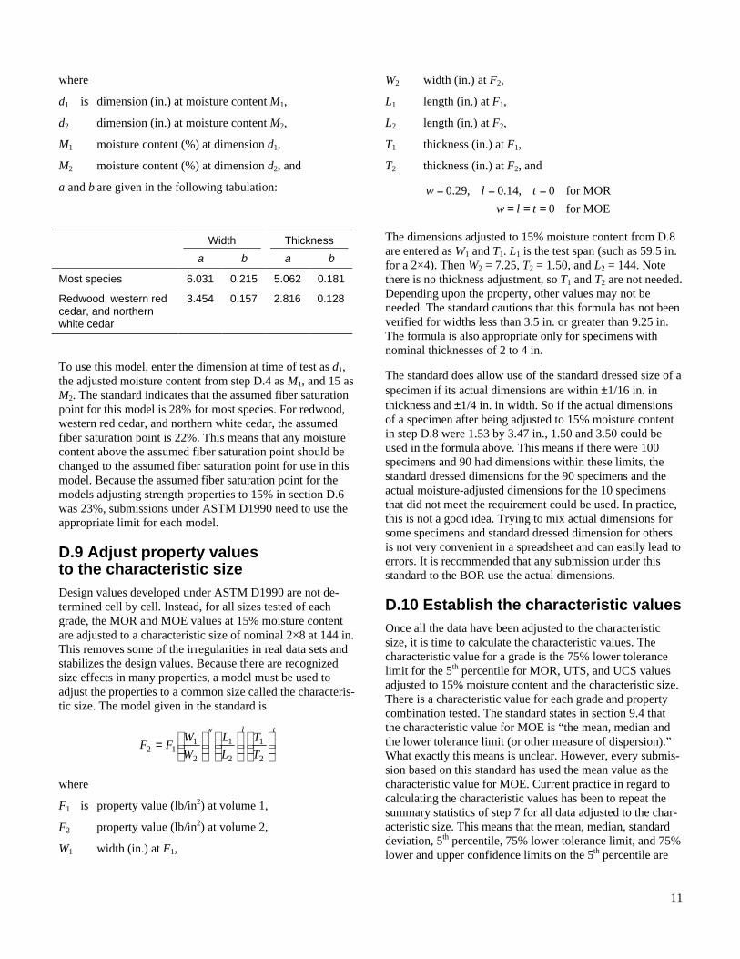
a and b are given in the following tabulation:

Width Thickness

a b a b

Most species 6.031 0.215 5.062 0.181

Redwood, western red cedar, and northern white cedar

3.454 0.157 2.816 0.128

To use this model, enter the dimension at time of test as d1, the adjusted moisture content from step D.4 as M1, and 15 as M2. The standard indicates that the assumed fiber saturation point for this model is 28% for most species. For redwood, western red cedar, and northern white cedar, the assumed fiber saturation point is 22%. This means that any moisture content above the assumed fiber saturation point should be changed to the assumed fiber saturation point for use in this model. Because the assumed fiber saturation point for the models adjusting strength properties to 15% in section D.6 was 23%, submissions under ASTM D1990 need to use the appropriate limit for each model.

D.9 Adjust property values to the characteristic size Design values developed under ASTM D1990 are not de-termined cell by cell. Instead, for all sizes tested of each grade, the MOR and MOE values at 15% moisture content are adjusted to a characteristic size of nominal 2×8 at 144 in. This removes some of the irregularities in real data sets and stabilizes the design values. Because there are recognized size effects in many properties, a model must be used to adjust the properties to a common size called the characteris-tic size. The model given in the standard is

tlw

T

T

L

L

W

WFF

=

2

1

2

1

2

112

where

F1 is property value (lb/in2) at volume 1,

F2 property value (lb/in2) at volume 2,

W1 width (in.) at F1,

W2 width (in.) at F2,

L1 length (in.) at F1,

L2 length (in.) at F2,

T1 thickness (in.) at F1,

T2 thickness (in.) at F2, and

for MOE0

for MOR0,14.0,29.0

======

tlw

tlw

The dimensions adjusted to 15% moisture content from D.8 are entered as W1 and T1. L1 is the test span (such as 59.5 in. for a 2×4). Then W2 = 7.25, T2 = 1.50, and L2 = 144. Note there is no thickness adjustment, so T1 and T2 are not needed. Depending upon the property, other values may not be needed. The standard cautions that this formula has not been verified for widths less than 3.5 in. or greater than 9.25 in. The formula is also appropriate only for specimens with nominal thicknesses of 2 to 4 in.

The standard does allow use of the standard dressed size of a specimen if its actual dimensions are within ±1/16 in. in thickness and ±1/4 in. in width. So if the actual dimensions of a specimen after being adjusted to 15% moisture content in step D.8 were 1.53 by 3.47 in., 1.50 and 3.50 could be used in the formula above. This means if there were 100 specimens and 90 had dimensions within these limits, the standard dressed dimensions for the 90 specimens and the actual moisture-adjusted dimensions for the 10 specimens that did not meet the requirement could be used. In practice, this is not a good idea. Trying to mix actual dimensions for some specimens and standard dressed dimension for others is not very convenient in a spreadsheet and can easily lead to errors. It is recommended that any submission under this standard to the BOR use the actual dimensions.

D.10 Establish the characteristic values Once all the data have been adjusted to the characteristic size, it is time to calculate the characteristic values. The characteristic value for a grade is the 75% lower tolerance limit for the 5th percentile for MOR, UTS, and UCS values adjusted to 15% moisture content and the characteristic size. There is a characteristic value for each grade and property combination tested. The standard states in section 9.4 that the characteristic value for MOE is “the mean, median and the lower tolerance limit (or other measure of dispersion).” What exactly this means is unclear. However, every submis-sion based on this standard has used the mean value as the characteristic value for MOE. Current practice in regard to calculating the characteristic values has been to repeat the summary statistics of step 7 for all data adjusted to the char-acteristic size. This means that the mean, median, standard deviation, 5th percentile, 75% lower tolerance limit, and 75% lower and upper confidence limits on the 5th percentile are

12

available for every property. The characteristic values are then readily availble to be used to develop design values.

D.11 Conduct the section 9.3 and section 12.6 data checks To ensure that the resulting design values are not substan-tially greater than the experimental data obtained for any size–grade cell, two data checks are included in the standard. These data checks are performed on MOR, UTS, and UCS. There is no data check for MOE.

D.11.1 The section 9.3 data check The first data check is given in section 9.3 of the standard. To perform this check, the characteristic value for each grade is entered into the size model of step D.9 and adjusted to each size of each grade tested. It is compared to the 75% upper confidence limit on the 5th percentile of the data in the cell. This value is part of the summary statistics calculated in step D.7. If the adjusted characteristic value for each grade is below the 75% upper confidence limit on the 5th percentile in every size tested in that grade, the characteristic value passes the check and nothing is done. If the adjusted characteristic value is above the 75% upper confidence limit for any given size, the grade’s characteristic value is lowered to a value at which it will pass in every size cell of that grade. For exam-ple, suppose for MOR the Select Structural characteristic value is 2,988 lb/in2 and the 2×4 Select Structural 75% upper confidence limit on the 5th percentile is 4,107 lb/in2. Using the size model to adjust the characteristic value from a width of 7.25 in. and a length of 144 in. to a width of 3.50 in. and a length of 60 in. (assuming testing was at about a 17-to-1 span-to-depth ratio) gives a value of 4,172 lb/in2, which is greater than the 75% upper confidence limit of 4,107 lb/in2. The new characteristic value can be found by adjusting the 75% upper confidence limit on the 5th percentile to the char-acteristic size. Thus the characteristic value in the example would need to be lowered to 2,941 lb/in2.

D.11.2 Section 12.6 data check The next step is to perform the section 12.6 data check. To perform this check, the individual grade characteristic value resulting from the 9.3 data check are put back into the size model of step D.9 and adjusted to every size tested. These values are compared to the test cell nonparametric 5th percentile instead of the upper 75% confidence limit on the 5th percentile as in the 9.3 data check. If it is no more than 100 lb/in2 or 5% (whichever is smaller) above the 5th percentile, the value passes. However, if the value calculated from the characteristic value is too high, something must be done. In the In-Grade Program, the Southern Pine Inspection Bureau lowered the estimated property in the cells that failed. All other submissions in the In-Grade Program and subsequent submissions have lowered the characteristic values for a grade if any size cell in the grade failed the

12.6 check. This preserves the size effect curve in allowable properties that are developed and is the method that this report in subsequent discussion will assume is being used. To continue the example from above, suppose the 5th percen-tile of the 2×4 Select Structural data is 3,917 lb/in2. The 5th percentile plus 100 lb/in2 is 4,017 lb/in2, and 5% over the 5th percentile is 4,113 lb/in2. The smaller of these values is 4,017 lb/in2. As seen in the example of above, the estimated value for this cell based on the reduced characteristic value of 2,941 lb/in2 is 4,107 lb/in2, which is above the limits of the 12.6 data check. To pass the 12.6 data check, the charac-teristic value for this grade must be further reduced to 2,877 lb/in2.

Recent submissions of foreign species to the BOR have tested only properties in bending. The standard does contain a conservative procedure to estimate the characteristic values for properties not tested from the MOR characteristic value. The location of this conservative procedure in the standard and the standard’s flow diagram would imply that it be done before the 12.6 data check. However, if the characteristic values for properties not tested is estimated using the proce-dures of section 9.5.2 of ASTM D1990 and the MOR char-acteristic value is later lowered from the 12.6 data check, the other estimated characteristic values might not be conserva-tive. Therefore, all submissions to the BOR that have esti-mated characteristic values for untested properties have performed the 12.6 data check before estimating the charac-teristic values. Because any submission to the BOR is based in part on historical precedence, it is recommended to con-tinue the practice of performing the 12.6 data check before estimating other characteristic values.

D.12 Estimate characteristic values for untested properties Following the recommendation to do the 12.6 data check before calculating the characteristic values of untested prop-erties, it is now time to take the resulting characteristic value for MOR from the 12.6 data check and estimate characteris-tic values for UTS and UCS. The characteristic value for UTS (T) can be calculated from the characteristic value for MOR (R) using the formula

T = 0.45R

and the characteristic value for UCS (C) can be calculated from the characteristic value for MOR (R) using

200,739.0

200,7000,1

022.0000,1

32.055.12

>=

≤

+−=

RR

RRRR

C

where R is measured in pounds per square inch.

13

D.13 Develop allowable properties from the final characteristic values for a full sampling matrix At this point the final characteristic values are available for MOR, MOE, UTS, and UCS. A series of calculations, some of which are not specified in the standard, can convert these characteristic values into the allowable property values typically submitted to the BOR for a full sampling matrix. Each of the properties MOR, UTS, UCS, and MOE are discussed separately. The general procedure for MOR, UTS, and UCS follows four steps:

1. Get final characteristic values for every grade at the characteristic size (1.5 by 7.25 by 144 in.).

2. Use the size models of section D.9 to adjust the final characteristic values to a set of specific different sizes.

3. Make some specific adjustments to these numbers for factor of safety and DOL effects.

4. Round the values according to specified rounding rules.

MOE has a slightly different order of steps, which are dis-cussed later.

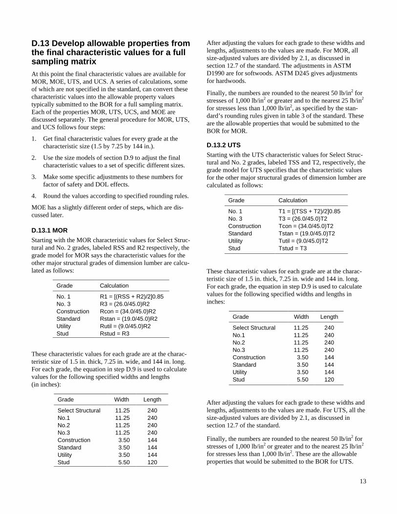
D.13.1 MOR Starting with the MOR characteristic values for Select Struc-tural and No. 2 grades, labeled RSS and R2 respectively, the grade model for MOR says the characteristic values for the other major structural grades of dimension lumber are calcu-lated as follows:

Grade Calculation

No. 1 R1 = [(RSS + R2)/2]0.85 No. 3 R3 = (26.0/45.0)R2 Construction Rcon = (34.0/45.0)R2 Standard Rstan = (19.0/45.0)R2 Utility Rutil = (9.0/45.0)R2 Stud Rstud = R3

These characteristic values for each grade are at the charac-teristic size of 1.5 in. thick, 7.25 in. wide, and 144 in. long. For each grade, the equation in step D.9 is used to calculate values for the following specified widths and lengths (in inches):

Grade Width Length

Select Structural 11.25 240 No.1 11.25 240 No.2 11.25 240 No.3 11.25 240 Construction 3.50 144 Standard 3.50 144 Utility 3.50 144 Stud 5.50 120

After adjusting the values for each grade to these widths and lengths, adjustments to the values are made. For MOR, all size-adjusted values are divided by 2.1, as discussed in section 12.7 of the standard. The adjustments in ASTM D1990 are for softwoods. ASTM D245 gives adjustments for hardwoods.

Finally, the numbers are rounded to the nearest 50 lb/in2 for stresses of 1,000 lb/in2 or greater and to the nearest 25 lb/in2 for stresses less than 1,000 lb/in2, as specified by the stan-dard’s rounding rules given in table 3 of the standard. These are the allowable properties that would be submitted to the BOR for MOR.

D.13.2 UTS Starting with the UTS characteristic values for Select Struc-tural and No. 2 grades, labeled TSS and T2, respectively, the grade model for UTS specifies that the characteristic values for the other major structural grades of dimension lumber are calculated as follows:

Grade Calculation

No. 1 T1 = [(TSS + T2)/2]0.85 No. 3 T3 = (26.0/45.0)T2 Construction Tcon = (34.0/45.0)T2 Standard Tstan = (19.0/45.0)T2 Utility Tutil = (9.0/45.0)T2 Stud Tstud = T3

These characteristic values for each grade are at the charac-teristic size of 1.5 in. thick, 7.25 in. wide and 144 in. long. For each grade, the equation in step D.9 is used to calculate values for the following specified widths and lengths in inches:

Grade Width Length

Select Structural 11.25 240 No.1 11.25 240 No.2 11.25 240 No.3 11.25 240 Construction 3.50 144 Standard 3.50 144 Utility 3.50 144 Stud 5.50 120

After adjusting the values for each grade to these widths and lengths, adjustments to the values are made. For UTS, all the size-adjusted values are divided by 2.1, as discussed in section 12.7 of the standard.

Finally, the numbers are rounded to the nearest 50 lb/in2 for stresses of 1,000 lb/in2 or greater and to the nearest 25 lb/in2 for stresses less than 1,000 lb/in2. These are the allowable properties that would be submitted to the BOR for UTS.

14

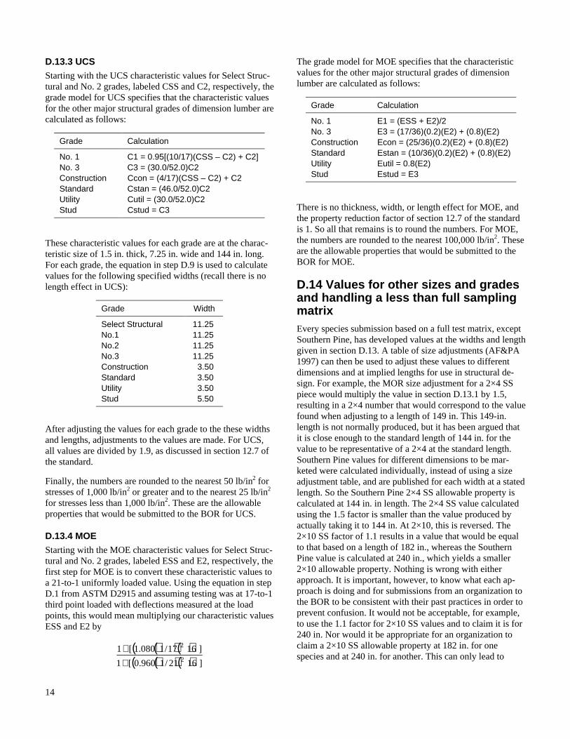
D.13.3 UCS Starting with the UCS characteristic values for Select Struc-tural and No. 2 grades, labeled CSS and C2, respectively, the grade model for UCS specifies that the characteristic values for the other major structural grades of dimension lumber are calculated as follows:

Grade Calculation

No. 1 C1 = 0.95[(10/17)(CSS – C2) + C2] No. 3 C3 = (30.0/52.0)C2 Construction Ccon = (4/17)(CSS – C2) + C2 Standard Cstan = (46.0/52.0)C2 Utility Cutil = (30.0/52.0)C2 Stud Cstud = C3

These characteristic values for each grade are at the charac-teristic size of 1.5 in. thick, 7.25 in. wide and 144 in. long. For each grade, the equation in step D.9 is used to calculate values for the following specified widths (recall there is no length effect in UCS):

Grade Width

Select Structural 11.25 No.1 11.25 No.2 11.25 No.3 11.25 Construction 3.50 Standard 3.50 Utility 3.50 Stud 5.50

After adjusting the values for each grade to the these widths and lengths, adjustments to the values are made. For UCS, all values are divided by 1.9, as discussed in section 12.7 of the standard.

Finally, the numbers are rounded to the nearest 50 lb/in2 for stresses of 1,000 lb/in2 or greater and to the nearest 25 lb/in2 for stresses less than 1,000 lb/in2. These are the allowable properties that would be submitted to the BOR for UCS.

D.13.4 MOE Starting with the MOE characteristic values for Select Struc-tural and No. 2 grades, labeled ESS and E2, respectively, the first step for MOE is to convert these characteristic values to a 21-to-1 uniformly loaded value. Using the equation in step D.1 from ASTM D2915 and assuming testing was at 17-to-1 third point loaded with deflections measured at the load points, this would mean multiplying our characteristic values ESS and E2 by

( )( ) ( )( )( ) ( )]1621/1960.0[1

]1617/1080.1[12

2

++

The grade model for MOE specifies that the characteristic values for the other major structural grades of dimension lumber are calculated as follows:

Grade Calculation

No. 1 E1 = (ESS + E2)/2 No. 3 E3 = (17/36)(0.2)(E2) + (0.8)(E2) Construction Econ = (25/36)(0.2)(E2) + (0.8)(E2) Standard Estan = (10/36)(0.2)(E2) + (0.8)(E2) Utility Eutil = 0.8(E2) Stud Estud = E3

There is no thickness, width, or length effect for MOE, and the property reduction factor of section 12.7 of the standard is 1. So all that remains is to round the numbers. For MOE, the numbers are rounded to the nearest 100,000 lb/in2. These are the allowable properties that would be submitted to the BOR for MOE.

D.14 Values for other sizes and grades and handling a less than full sampling matrix Every species submission based on a full test matrix, except Southern Pine, has developed values at the widths and length given in section D.13. A table of size adjustments (AF&PA 1997) can then be used to adjust these values to different dimensions and at implied lengths for use in structural de-sign. For example, the MOR size adjustment for a 2×4 SS piece would multiply the value in section D.13.1 by 1.5, resulting in a 2×4 number that would correspond to the value found when adjusting to a length of 149 in. This 149-in. length is not normally produced, but it has been argued that it is close enough to the standard length of 144 in. for the value to be representative of a 2×4 at the standard length. Southern Pine values for different dimensions to be mar-keted were calculated individually, instead of using a size adjustment table, and are published for each width at a stated length. So the Southern Pine 2×4 SS allowable property is calculated at 144 in. in length. The 2×4 SS value calculated using the 1.5 factor is smaller than the value produced by actually taking it to 144 in. At 2×10, this is reversed. The 2×10 SS factor of 1.1 results in a value that would be equal to that based on a length of 182 in., whereas the Southern Pine value is calculated at 240 in., which yields a smaller 2×10 allowable property. Nothing is wrong with either approach. It is important, however, to know what each ap-proach is doing and for submissions from an organization to the BOR to be consistent with their past practices in order to prevent confusion. It would not be acceptable, for example, to use the 1.1 factor for 2×10 SS values and to claim it is for 240 in. Nor would it be appropriate for an organization to claim a 2×10 SS allowable property at 182 in. for one species and at 240 in. for another. This can only lead to

15

confusion in designing with wood. Finally, because all sub-missions, except Southern Pine, have used the factor ap-proach, it would seem reasonable to standardize on it to further remove confusion in designing with wood.

The difference in these two approaches is important when dealing with less than the full sampling matrix discussed in section C.2. For example, with only one grade of material but three sizes, allowable properties can be calculated for all sizes of that grade using either the factors found in the size adjustment tables (AF&PA 1997) or by adjusting to a claimed length. Because rounding of values for less than a full matrix usually occurs after the size adjustment, consis-tency would appear to be important. Going to 149 in. for 2×4s of one species by using the 1.5 factor and going to 144 in. with the size model of step D.9 (which produces a factor of 1.507) for a different species could look like an attempt to be able to round a species up instead of down. In an effort to address this issue, the BOR recently decided that submis-sions of less than full matrices would be for set lengths. The lengths chosen are as follows:

Size Length

2×4 144 2×6 144 2×8 144 2×10 192 2×12 240

This ensures consistency with future submissions tested with less than a full matrix, but there could be an inconsistency between two species with exactly the same final values at the end of the calculations of section D.13.1, as in the following example: Suppose species A was tested with a full matrix, and species B was tested only with 2×4s. Both species have a select structural MOR of 4.872 × 103 lb/in2 after taking the value to 2×12 at 240 in. long. For species A, this value is divided by 2.1 to give 2.320 and rounded to 2.300. Someone designing anything with a 2×4 for species A would use 1.5 times 2.300, which is 3.450 × 103 lb/in2. However, for spe-cies B, the 4.872 value is adjusted to 2×4 at 144 in. (using the factor of 1.507), giving 7.342, which when divided by 2.1 to yield 3.496. This is rounded to 3.500 as an allowable 2×4 number and used as a design value for species B 2×4s. Some of this difference is due to the point at which rounding of values occurs and some to the difference in factors 1.5 and 1.507. In the interest of consistency, allowable prop-erties for partial matrices should probably still be given at the dimensions and lengths of full matrix submissions with a footnote indicating that the allowable properties can be used only when designing for the sampling matrix actually tested. Using the factors for consistency would eliminate differ-ences in implied lengths.

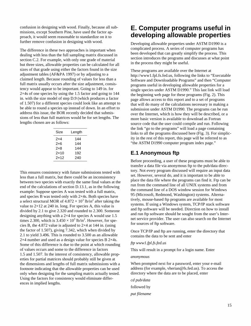
E. Computer programs useful in developing allowable properties Developing allowable properties under ASTM D1990 is a complicated process. A series of computer programs has been developed that can greatly simplify the process. This section introduces the programs and discusses at what point in the process they might be useful.

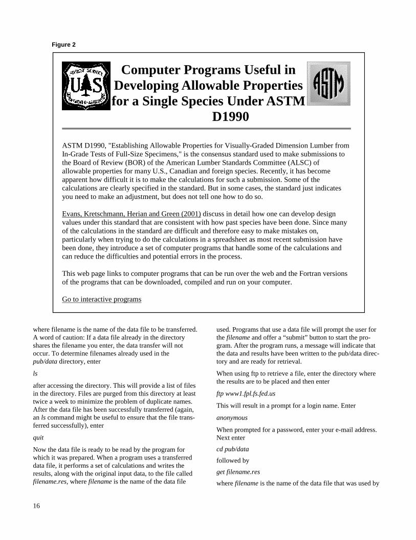
These programs are available over the Internet at http://www1.fpl.fs.fed.us, following the links to “Executable Software and Downloadable Programs” and then “Computer programs useful in developing allowable properties for a single species under ASTM D1990.” This last link will load the beginning web page for these programs (Fig. 2). This page allows access to this report and to a set of programs that will do many of the calculations necessary in making a submission under ASTM D1990. The programs can be run over the Internet, which is how they will be described, or a more basic version is available to download as Fortran source code that the user could compile and run. Following the link “go to the programs” will load a page containing links to all the programs discussed here (Fig. 3). For simplic-ity in the rest of this report, this page will be referred to as “the ASTM D1990 computer program index page.”

E.1 Anonymous ftp Before proceeding, a user of these programs must be able to transfer a data file via anonymous ftp to the pub/data direc-tory. Not every program discussed will require an input data set. However, several do, and it is important to be able to place the data file where the programs can find it. Ftp can be run from the command line of all UNIX systems and from the command line of a DOS window session for Windows 95 (Microsoft, Redmond, Washington) systems. Alterna-tively, mouse-based ftp programs are available for most systems. If using a Windows system, TCP/IP stack software and ftp software will be needed. Direction on how to install and run ftp software should be sought from the user’s Inter-net service provider. The user can also search on the Internet for sources of ftp software.

Once TCP/IP and ftp are running, enter the directory that contains the data to be sent and enter

ftp www1.fpl.fs.fed.us

This will result in a prompt for a login name. Enter

anonymous

When prompted next for a password, enter your e-mail address (for example, vherian@fs.fed.us). To access the directory where the data are to be placed, enter

cd pub/data

followed by

put filename

16

Figure 2

where filename is the name of the data file to be transferred. A word of caution: If a data file already in the directory shares the filename you enter, the data transfer will not occur. To determine filenames already used in the pub/data directory, enter

ls

after accessing the directory. This will provide a list of files in the directory. Files are purged from this directory at least twice a week to minimize the problem of duplicate names. After the data file has been successfully transferred (again, an ls command might be useful to ensure that the file trans-ferred successfully), enter

quit

Now the data file is ready to be read by the program for which it was prepared. When a program uses a transferred data file, it performs a set of calculations and writes the results, along with the original input data, to the file called filename.res, where filename is the name of the data file

used. Programs that use a data file will prompt the user for the filename and offer a “submit” button to start the pro-gram. After the program runs, a message will indicate that the data and results have been written to the pub/data direc-tory and are ready for retrieval.

When using ftp to retrieve a file, enter the directory where the results are to be placed and then enter

ftp www1.fpl.fs.fed.us

This will result in a prompt for a login name. Enter

anonymous

When prompted for a password, enter your e-mail address. Next enter

cd pub/data

followed by

get filename.res

where filename is the name of the data file that was used by

Computer Programs Useful in Developing Allowable Properties for a Single Species Under ASTM

D1990

ASTM D1990, "Establishing Allowable Properties for Visually-Graded Dimension Lumber from In-Grade Tests of Full-Size Specimens," is the consensus standard used to make submissions to the Board of Review (BOR) of the American Lumber Standards Committee (ALSC) of allowable properties for many U.S., Canadian and foreign species. Recently, it has become apparent how difficult it is to make the calculations for such a submission. Some of the calculations are clearly specified in the standard. But in some cases, the standard just indicates you need to make an adjustment, but does not tell one how to do so.

Evans, Kretschmann, Herian and Green (2001) discuss in detail how one can develop design values under this standard that are consistent with how past species have been done. Since many of the calculations in the standard are difficult and therefore easy to make mistakes on, particularly when trying to do the calculations in a spreadsheet as most recent submission have been done, they introduce a set of computer programs that handle some of the calculations and can reduce the difficulties and potential errors in the process.

This web page links to computer programs that can be run over the web and the Fortran versions of the programs that can be downloaded, compiled and run on your computer.

Go to interactive programs

17

Figure 3

the program. After the data transfer has been completed, exit ftp by typing

quit

The data file returned will contain all the original informa-tion plus an appended column(s) (depending on the pro-gram) of calculated information.

E.2 Grade quality index (strength ratio) program SRATIO Section C of this report discusses the importance of obtain-ing a representative sample and the concept of a grade quality index. As previously mentioned, all submissions to the BOR have used strength ratios calculated from failure codes as GQI values. The GQI program calculates strength ratios from failure codes found in table X1.1 of ASTM D4761. The program expects a failure code of the form XX−YY where XX is the two digit code showing the char-acteristic associated with the failure and YY is the two digit code describing the extent of this characteristic, as discussed

in ASTM D4761. It does not calculate a strength ratio for every failure code in ASTM D4761. The codes for which it will calculate strength ratios and the formulas it uses are discussed in Appendix 2.

E.2.1 Ftp data format The input data should be in the following format:

Columns 1–10 Specimen ID

Columns 12–16 Specimen thickness (in.) (for example, 1.540)

Columns 18–23 Specimen width (in.) (for example, 3.541)

Columns 27–28 Two-digit characteristic code (for example, 17 for an edge of wide face knot)

Columns 30–31 Two-digit size of characteristic code (for example, 08 for ½-in. edge of wide face knot)

Interactive Computer Programs Useful in Developing Allowable Properties Under

ASTM D1990

DISCLAIMER: These programs are meant to be an aid to people developing design values under ASTM D-1990. Many of them are still in development, so we can take no responsibility for any results that you get from using them. If you find what you perceive as an error in a program, please let us know so that we can continue to improve these programs.

SRATIO - a program to calculate strength ratios from failure codes

TEMPADJ - a program to adjust specimen properties from one temperature to another

MCADJ - a program to adjust specimen properties from one moisture content to another

NONPAR - a program to calculate nonparametric percentile estimates, tolerance limits and confidence intervals for percentiles

DATACHECK - a program to do the 9.3 and 12.6 datachecks

ALLFROMR - a program to calculate MOR, UTS, and UCS design values from MOR characteristic values

EDESIGN - a program to calculate MOE design values from MOE characteristic values

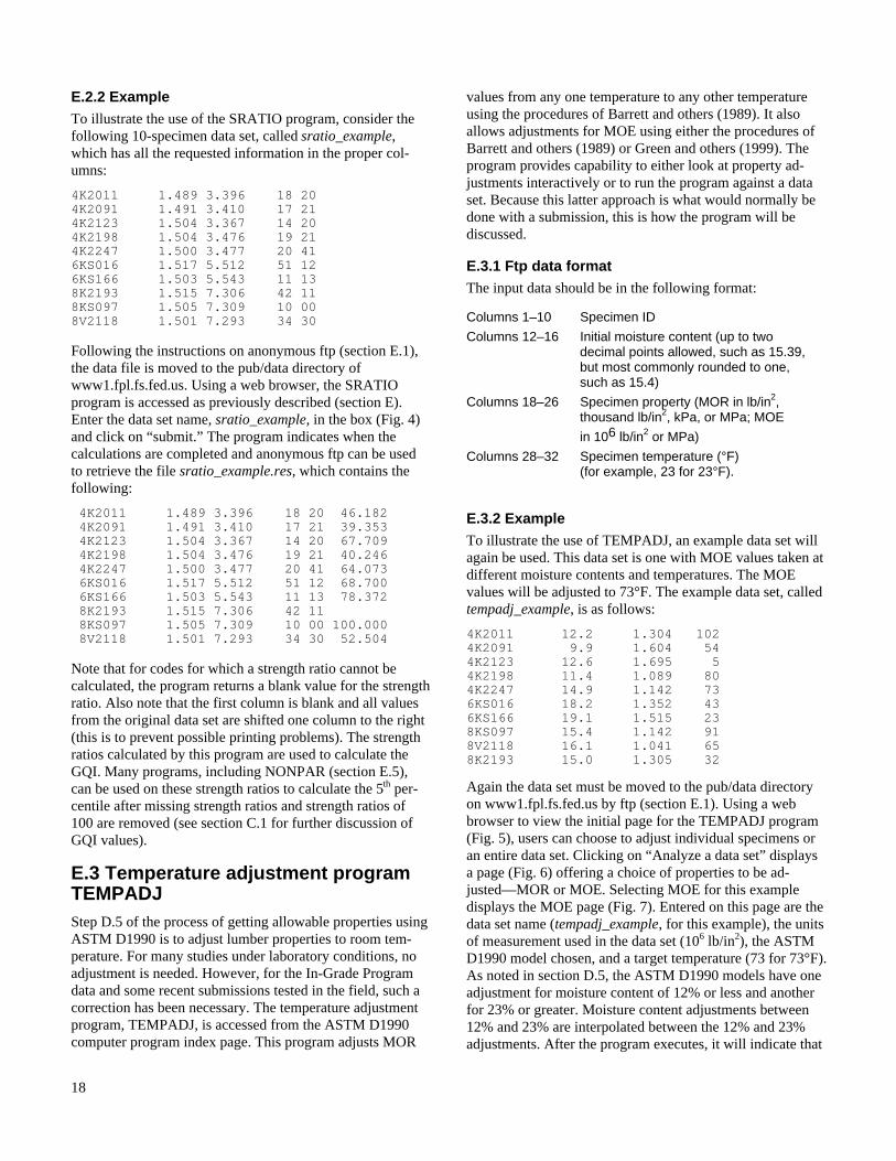
18

E.2.2 Example To illustrate the use of the SRATIO program, consider the following 10-specimen data set, called sratio_example, which has all the requested information in the proper col-umns:

4K2011 1.489 3.396 18 20 4K2091 1.491 3.410 17 21 4K2123 1.504 3.367 14 20 4K2198 1.504 3.476 19 21 4K2247 1.500 3.477 20 41 6KS016 1.517 5.512 51 12 6KS166 1.503 5.543 11 13 8K2193 1.515 7.306 42 11 8KS097 1.505 7.309 10 00 8V2118 1.501 7.293 34 30

Following the instructions on anonymous ftp (section E.1), the data file is moved to the pub/data directory of www1.fpl.fs.fed.us. Using a web browser, the SRATIO program is accessed as previously described (section E). Enter the data set name, sratio_example, in the box (Fig. 4) and click on “submit.” The program indicates when the calculations are completed and anonymous ftp can be used to retrieve the file sratio_example.res, which contains the following:

4K2011 1.489 3.396 18 20 46.182 4K2091 1.491 3.410 17 21 39.353 4K2123 1.504 3.367 14 20 67.709 4K2198 1.504 3.476 19 21 40.246 4K2247 1.500 3.477 20 41 64.073 6KS016 1.517 5.512 51 12 68.700 6KS166 1.503 5.543 11 13 78.372 8K2193 1.515 7.306 42 11 8KS097 1.505 7.309 10 00 100.000 8V2118 1.501 7.293 34 30 52.504

Note that for codes for which a strength ratio cannot be calculated, the program returns a blank value for the strength ratio. Also note that the first column is blank and all values from the original data set are shifted one column to the right (this is to prevent possible printing problems). The strength ratios calculated by this program are used to calculate the GQI. Many programs, including NONPAR (section E.5), can be used on these strength ratios to calculate the 5th per-centile after missing strength ratios and strength ratios of 100 are removed (see section C.1 for further discussion of GQI values).

E.3 Temperature adjustment program TEMPADJ Step D.5 of the process of getting allowable properties using ASTM D1990 is to adjust lumber properties to room tem-perature. For many studies under laboratory conditions, no adjustment is needed. However, for the In-Grade Program data and some recent submissions tested in the field, such a correction has been necessary. The temperature adjustment program, TEMPADJ, is accessed from the ASTM D1990 computer program index page. This program adjusts MOR

values from any one temperature to any other temperature using the procedures of Barrett and others (1989). It also allows adjustments for MOE using either the procedures of Barrett and others (1989) or Green and others (1999). The program provides capability to either look at property ad-justments interactively or to run the program against a data set. Because this latter approach is what would normally be done with a submission, this is how the program will be discussed.

E.3.1 Ftp data format The input data should be in the following format:

Columns 1–10 Specimen ID

Columns 12–16 Initial moisture content (up to two decimal points allowed, such as 15.39, but most commonly rounded to one, such as 15.4)

Columns 18–26 Specimen property (MOR in lb/in2, thousand lb/in2, kPa, or MPa; MOE

in 106 lb/in2 or MPa)

Columns 28–32 Specimen temperature (°F) (for example, 23 for 23°F).

E.3.2 Example To illustrate the use of TEMPADJ, an example data set will again be used. This data set is one with MOE values taken at different moisture contents and temperatures. The MOE values will be adjusted to 73°F. The example data set, called tempadj_example, is as follows:

4K2011 12.2 1.304 102 4K2091 9.9 1.604 54 4K2123 12.6 1.695 5 4K2198 11.4 1.089 80 4K2247 14.9 1.142 73 6KS016 18.2 1.352 43 6KS166 19.1 1.515 23 8KS097 15.4 1.142 91 8V2118 16.1 1.041 65 8K2193 15.0 1.305 32

Again the data set must be moved to the pub/data directory on www1.fpl.fs.fed.us by ftp (section E.1). Using a web browser to view the initial page for the TEMPADJ program (Fig. 5), users can choose to adjust individual specimens or an entire data set. Clicking on “Analyze a data set” displays a page (Fig. 6) offering a choice of properties to be ad-justed—MOR or MOE. Selecting MOE for this example displays the MOE page (Fig. 7). Entered on this page are the data set name (tempadj_example, for this example), the units of measurement used in the data set (106 lb/in2), the ASTM D1990 model chosen, and a target temperature (73 for 73°F). As noted in section D.5, the ASTM D1990 models have one adjustment for moisture content of 12% or less and another for 23% or greater. Moisture content adjustments between 12% and 23% are interpolated between the 12% and 23% adjustments. After the program executes, it will indicate that

19

Figure 4

WWW Computer Program for Calculating Strength Ratios from Failure Codes in ASTM

D4761, Table X1.1.

This program calculates strength ratios from failure codes in ASTM D 4761 Table X1.1. These codes are of the form 'XX-YY', where XX is a 2-digit code showing the characteristic associated with a failure and YY is a 2-digit code describing the extent of the characteristic. Some examples are: 15-08 is a 1/2 inch wide face knot, center line encased. 51-12 is slope of grain 1 inch for every 12 inches. See ASTM D 4761 Table X1.1 for a complete list of failure codes.

This program will read a data set with the following format:

• Columns 1-10 contain a specimen id • Coluumns 12-16 contain the specimen thickness in inches (e.g., 1.540) • Columns 18-23 contain the specimen width in inches (e.g., 3.541) • Columns 27-28 contain the 2-digit characteristic code (e.g., 17 for an edge of wide face

knot) • Columns 30-31 contain the 2-digit size of characteristic code (e.g., 08 for 1/2-inch edge

of wide face knot)

WARNING!! You must have data for each variable. If data is missing, you must enter a period ( . ) to hold its place. If not, the program will put a 0.000 in its place when it writes out the results. This could cause you further problems in future calculations.

Before you proceed, you must transfer this datafile to ws13.fpl.fs.fed.us via anonymous ftp. You must place it in the pub/data directory. (If ftp does not run on your machine, e-mail your data to the address given below and it will be placed in the directory.)

The program will calculate a strength ratio for each specimen, and write it out, along with your original input data, to a file that has your original filename with an extension of .res added to it. (For example, if you sent a data set called himom, you will get back a data set called himom.res.) You can then retrieve your file via anonymous ftp from the pub/data directory.

Please enter the name of the data set you have put in our /pub/data directory for which you would like estimated percentiles.

sratio_example

Submit Clear Form

20

Figure 5

Figure 6

Input From Your Data Set

Which property would you like to adjust? (Available models follow the property choice.)

• Modulus of Rupture (ASTM D-1990) • Modulus of Elasticity (ASTM D-1990, New MOE Model)

WWW Computer Program for Adjusting Mechanical Properties

of Dimension Lumber for Changes in Temperature

This program calculates changes in dimension lumber properties associated with changes in temperature.

• Modulus of Rupture (ASTM D-1990) • Modulus of Elasticity (ASTM D-1990, New MOE Model)

You may choose either of the following methods of running the program:

• Individual piece or property - Interactive input from keyboard • Analyze a data set via anonymous ftp

21

Figure 7

MODULUS OF Elasticity (MOE) (From Your Data Set)

Format of Your Data - Your data should be in the following format:

• Columns 1-10 contain a specimen id • Columns 12-16 contain the initial moisture content (i.e. 15.00 or 15.0) • Columns 18-26 contain the specimen property (in106psi or MPa) • Columns 28-32 contain the temperature ( degrees in Fahrenheit, i.e., 23)

WARNING!! You must have data for each variable. If data is missing, you must enter a period ( . ) to hold its place. If not, the program will put a 0.000 in its place when it writes out the results. This could cause you further problems in future calculations.

Before you proceed, you must transfer this datafile to ws13.fpl.fs.fed.us via anonymous ftp. You must place it in the pub/data directory. (If ftp does not run on your machine, e-mail your data to the address given below and it will be placed in the directory.)

The program will calculate an adjusted MOE for the targeted temperature for each specimen, and write it out, along with your original input data, to a file that has your original filename with an extension .res added to it. (For example, if you sent a data set called himom, you will get back a data set called himom.res.) You can then retrieve your file via anonymous ftp from the pub/data directory.

Please enter the name of the data set you have put in our /pub/data directory for which

you would like adjusted MOE values. tempadj_example

Initial Property Value Format (PICK ONE) � �� �� �

106psi (e.g., 1.8711) � ��

MPa (e.g., 12900)

Please pick one model � � �� �

ASTM D-1990 Model � �� ��

New MOE Model

Please Enter Your Target Temperature � �� �� �

Fahrenheit � �� �

Centigrade 73

Submit Clear Form

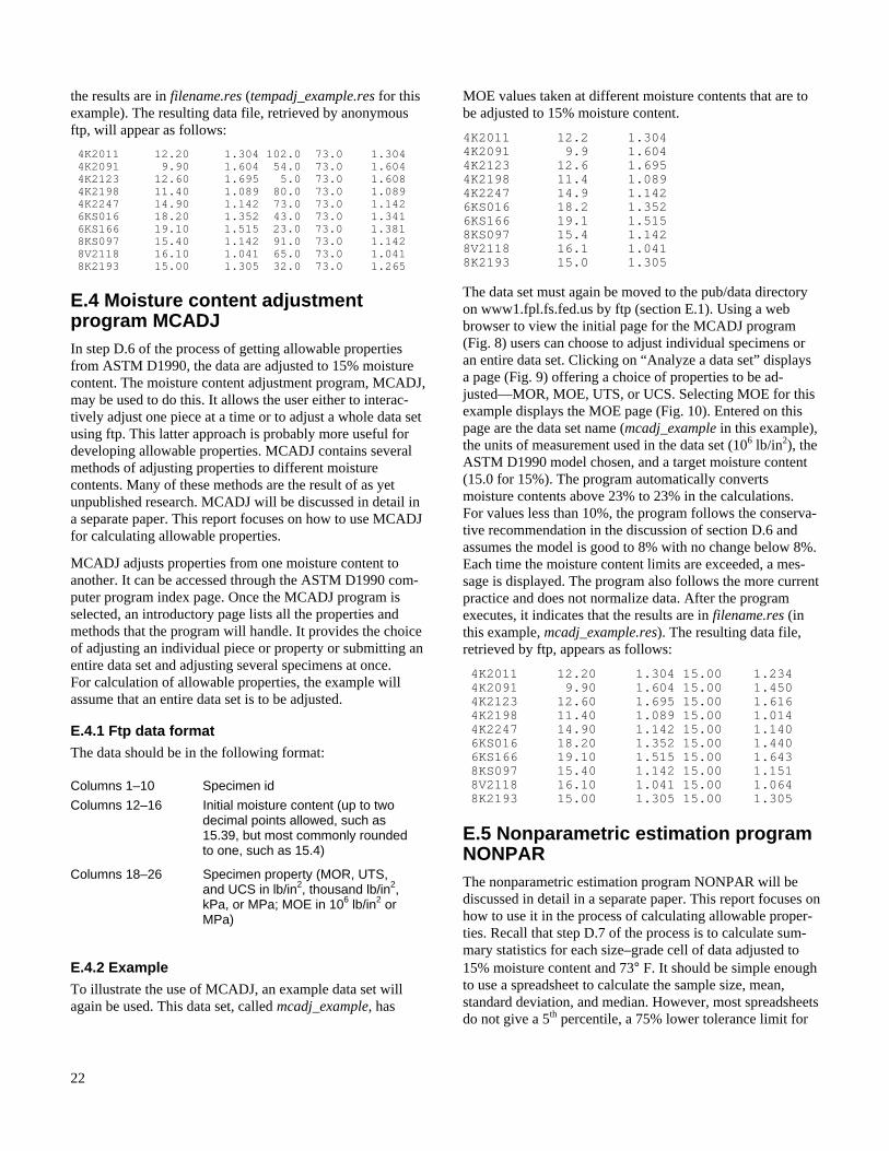
22

the results are in filename.res (tempadj_example.res for this example). The resulting data file, retrieved by anonymous ftp, will appear as follows:

4K2011 12.20 1.304 102.0 73.0 1.304 4K2091 9.90 1.604 54.0 73.0 1.604 4K2123 12.60 1.695 5.0 73.0 1.608 4K2198 11.40 1.089 80.0 73.0 1.089 4K2247 14.90 1.142 73.0 73.0 1.142 6KS016 18.20 1.352 43.0 73.0 1.341 6KS166 19.10 1.515 23.0 73.0 1.381 8KS097 15.40 1.142 91.0 73.0 1.142 8V2118 16.10 1.041 65.0 73.0 1.041 8K2193 15.00 1.305 32.0 73.0 1.265

E.4 Moisture content adjustment program MCADJ In step D.6 of the process of getting allowable properties from ASTM D1990, the data are adjusted to 15% moisture content. The moisture content adjustment program, MCADJ, may be used to do this. It allows the user either to interac-tively adjust one piece at a time or to adjust a whole data set using ftp. This latter approach is probably more useful for developing allowable properties. MCADJ contains several methods of adjusting properties to different moisture contents. Many of these methods are the result of as yet unpublished research. MCADJ will be discussed in detail in a separate paper. This report focuses on how to use MCADJ for calculating allowable properties.

MCADJ adjusts properties from one moisture content to another. It can be accessed through the ASTM D1990 com-puter program index page. Once the MCADJ program is selected, an introductory page lists all the properties and methods that the program will handle. It provides the choice of adjusting an individual piece or property or submitting an entire data set and adjusting several specimens at once. For calculation of allowable properties, the example will assume that an entire data set is to be adjusted.

E.4.1 Ftp data format The data should be in the following format:

Columns 1–10 Specimen id

Columns 12–16 Initial moisture content (up to two decimal points allowed, such as 15.39, but most commonly rounded to one, such as 15.4)

Columns 18–26 Specimen property (MOR, UTS, and UCS in lb/in2, thousand lb/in2, kPa, or MPa; MOE in 106 lb/in2 or MPa)

E.4.2 Example To illustrate the use of MCADJ, an example data set will again be used. This data set, called mcadj_example, has

MOE values taken at different moisture contents that are to be adjusted to 15% moisture content.

4K2011 12.2 1.304 4K2091 9.9 1.604 4K2123 12.6 1.695 4K2198 11.4 1.089 4K2247 14.9 1.142 6KS016 18.2 1.352 6KS166 19.1 1.515 8KS097 15.4 1.142 8V2118 16.1 1.041 8K2193 15.0 1.305

The data set must again be moved to the pub/data directory on www1.fpl.fs.fed.us by ftp (section E.1). Using a web browser to view the initial page for the MCADJ program (Fig. 8) users can choose to adjust individual specimens or an entire data set. Clicking on “Analyze a data set” displays a page (Fig. 9) offering a choice of properties to be ad-justed—MOR, MOE, UTS, or UCS. Selecting MOE for this example displays the MOE page (Fig. 10). Entered on this page are the data set name (mcadj_example in this example), the units of measurement used in the data set (106 lb/in2), the ASTM D1990 model chosen, and a target moisture content (15.0 for 15%). The program automatically converts moisture contents above 23% to 23% in the calculations. For values less than 10%, the program follows the conserva-tive recommendation in the discussion of section D.6 and assumes the model is good to 8% with no change below 8%. Each time the moisture content limits are exceeded, a mes-sage is displayed. The program also follows the more current practice and does not normalize data. After the program executes, it indicates that the results are in filename.res (in this example, mcadj_example.res). The resulting data file, retrieved by ftp, appears as follows:

4K2011 12.20 1.304 15.00 1.234 4K2091 9.90 1.604 15.00 1.450 4K2123 12.60 1.695 15.00 1.616 4K2198 11.40 1.089 15.00 1.014 4K2247 14.90 1.142 15.00 1.140 6KS016 18.20 1.352 15.00 1.440 6KS166 19.10 1.515 15.00 1.643 8KS097 15.40 1.142 15.00 1.151 8V2118 16.10 1.041 15.00 1.064 8K2193 15.00 1.305 15.00 1.305

E.5 Nonparametric estimation program NONPAR The nonparametric estimation program NONPAR will be discussed in detail in a separate paper. This report focuses on how to use it in the process of calculating allowable proper-ties. Recall that step D.7 of the process is to calculate sum-mary statistics for each size–grade cell of data adjusted to 15% moisture content and 73° F. It should be simple enough to use a spreadsheet to calculate the sample size, mean, standard deviation, and median. However, most spreadsheets do not give a 5th percentile, a 75% lower tolerance limit for

23

Figure 8

Figure 9

WWW Computer Program for Adjusting

Mechanical Properties of Dimension Lumber for Changes in Moisture Content

Lumber strength properties vary with changes in moisture content. This program allows you to predict a property (P2) of dimension lumber at a target moisture content (MC2) given that you know the value of the property (P1) at an initial moisture content (MC1). Properties and models for which this program provides estimates include:

• Modulus of Rupture (ASTM D-1990 and Quadratic Surface Models) • Modulus of Elasticity (ASTM D-1990, Simple Interest, and Compound Interest Models) • Ultimate Tensile Strength (ASTM D-1990 and Quadratic Surface Models) • Compression Parallel to the Grain (ASTM D-1990 and Quadratic Surface Models) • Compression Perpendicular to the Grain (ASTM D-2915) • Shear (ASTM D-2915)

You may choose either of the following methods of running the program:

• Individual piece or property - Interactive input from keyboard • Analyze a data set via anonymous ftp

Input From Your Data Set

Which property would you like to adjust? (Available models follow the property choice.)

• Modulus of Rupture (ASTM D-1990 and Quadratic Surface Models) • Modulus of Elasticity (ASTM D-1990, Simple Interest, and Compound Interest Models) • Ultimate Tensile Strength (ASTM D-1990 and Quadratic Surface Models) • Compression Parallel to the Grain (ASTM D-1990 and Quadratic Surface Models)

24

Figure 10

MODULUS OF Elasticity (MOE) (From Your Data Set)

Format of Your Data - Your data should be in the following format:

• Columns 1-10 contain a specimen id • Columns 12-16 contain the initial moisture content, i.e. 15.00 or 15.0 • Columns 18-26 contain the specimen property (in106psi or MPa) • No moisture content can be below 8.0 or above 23.0

WARNING!! You must have data for each variable. If data is missing, you must enter a period ( . ) to hold its place. If not, the program will put a 0.000 in its place when it writes out the results. This could cause you further problems in future calculations.

Before you proceed, you must transfer this datafile to ws10.fpl.fs.fed.us via anonymous ftp. You must place it in the pub/data directory. (If ftp does not run on your machine, e-mail your data to the address given below and it will be placed in the directory.)

The program will calculate an adjusted MOE for the targeted moisture content for each specimen, and write it out, along with your original input data, to a file that has your original filename with an extension .res added to it. (For example, if you sent a data set called himom, you will get back a data set called himom.res.) You can then retrieve your file via anonymous ftp from the pub/data directory.

Please enter the name of the data set you have put in our /pub/data directory for which

you would like adjusted MOE values. mcadj_example

Initial Property Value Format(PICK ONE) � �� �� �

106psi (e.g., 1.8711) � ��

MPa (e.g., 12900.090)

Please pick one model � � �� �

ASTM D-1990 Model � �� ��

Simple Interest Model � �� ��

Compound Interest Model

Please Enter Your Target Moisture Content (DO NOT USE %, USE 15.0 or 15.00,

for example) 15.0

Submit Clear Form

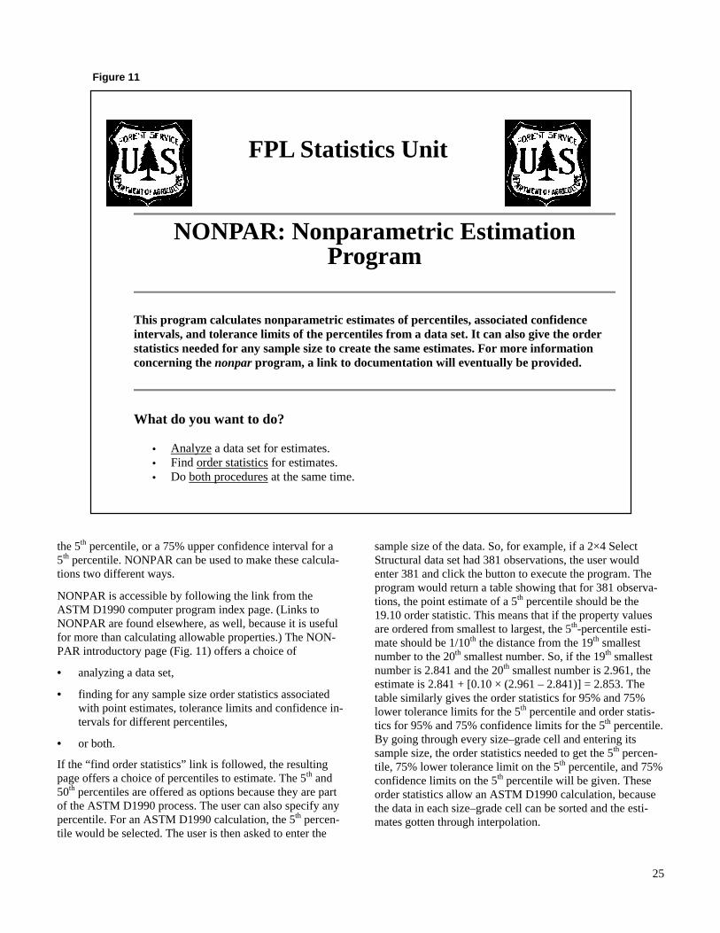
25

Figure 11

the 5th percentile, or a 75% upper confidence interval for a 5th percentile. NONPAR can be used to make these calcula-tions two different ways.

NONPAR is accessible by following the link from the ASTM D1990 computer program index page. (Links to NONPAR are found elsewhere, as well, because it is useful for more than calculating allowable properties.) The NON-PAR introductory page (Fig. 11) offers a choice of

• analyzing a data set,

• finding for any sample size order statistics associated with point estimates, tolerance limits and confidence in-tervals for different percentiles,

• or both.

If the “find order statistics” link is followed, the resulting page offers a choice of percentiles to estimate. The 5th and 50th percentiles are offered as options because they are part of the ASTM D1990 process. The user can also specify any percentile. For an ASTM D1990 calculation, the 5th percen-tile would be selected. The user is then asked to enter the

sample size of the data. So, for example, if a 2×4 Select Structural data set had 381 observations, the user would enter 381 and click the button to execute the program. The program would return a table showing that for 381 observa-tions, the point estimate of a 5th percentile should be the 19.10 order statistic. This means that if the property values are ordered from smallest to largest, the 5th-percentile esti-mate should be 1/10th the distance from the 19th smallest number to the 20th smallest number. So, if the 19th smallest number is 2.841 and the 20th smallest number is 2.961, the estimate is 2.841 + [0.10 × (2.961 – 2.841)] = 2.853. The table similarly gives the order statistics for 95% and 75% lower tolerance limits for the 5th percentile and order statis-tics for 95% and 75% confidence limits for the 5th percentile. By going through every size–grade cell and entering its sample size, the order statistics needed to get the 5th percen-tile, 75% lower tolerance limit on the 5th percentile, and 75% confidence limits on the 5th percentile will be given. These order statistics allow an ASTM D1990 calculation, because the data in each size–grade cell can be sorted and the esti-mates gotten through interpolation.

FPL Statistics Unit

NONPAR: Nonparametric Estimation Program

This program calculates nonparametric estimates of percentiles, associated confidence intervals, and tolerance limits of the percentiles from a data set. It can also give the order statistics needed for any sample size to create the same estimates. For more information concerning the nonpar program, a link to documentation will eventually be provided.

What do you want to do?

• Analyze a data set for estimates. • Find order statistics for estimates. • Do both procedures at the same time.

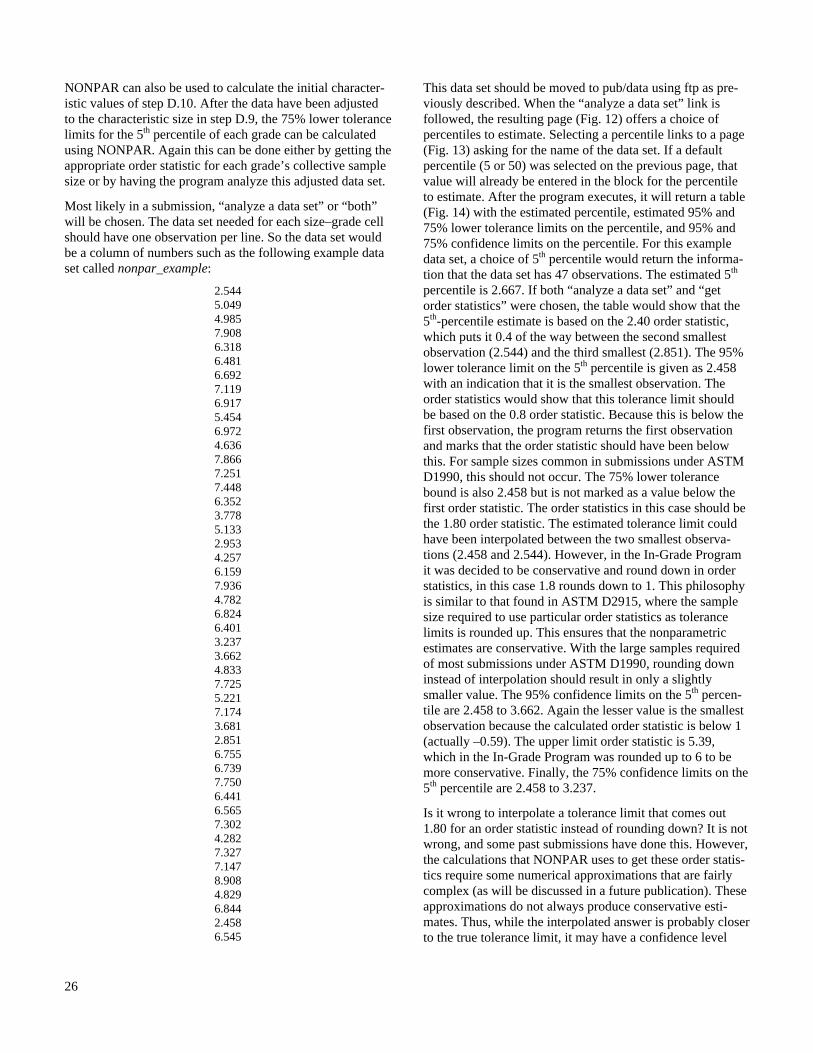
26

NONPAR can also be used to calculate the initial character-istic values of step D.10. After the data have been adjusted to the characteristic size in step D.9, the 75% lower tolerance limits for the 5th percentile of each grade can be calculated using NONPAR. Again this can be done either by getting the appropriate order statistic for each grade’s collective sample size or by having the program analyze this adjusted data set.

Most likely in a submission, “analyze a data set” or “both” will be chosen. The data set needed for each size–grade cell should have one observation per line. So the data set would be a column of numbers such as the following example data set called nonpar_example:

2.544 5.049 4.985 7.908 6.318 6.481 6.692 7.119 6.917 5.454 6.972 4.636 7.866 7.251 7.448 6.352 3.778 5.133 2.953 4.257 6.159 7.936 4.782 6.824 6.401 3.237 3.662 4.833 7.725 5.221 7.174 3.681 2.851 6.755 6.739 7.750 6.441 6.565 7.302 4.282 7.327 7.147 8.908 4.829 6.844 2.458 6.545

This data set should be moved to pub/data using ftp as pre-viously described. When the “analyze a data set” link is followed, the resulting page (Fig. 12) offers a choice of percentiles to estimate. Selecting a percentile links to a page (Fig. 13) asking for the name of the data set. If a default percentile (5 or 50) was selected on the previous page, that value will already be entered in the block for the percentile to estimate. After the program executes, it will return a table (Fig. 14) with the estimated percentile, estimated 95% and 75% lower tolerance limits on the percentile, and 95% and 75% confidence limits on the percentile. For this example data set, a choice of 5th percentile would return the informa-tion that the data set has 47 observations. The estimated 5th percentile is 2.667. If both “analyze a data set” and “get order statistics” were chosen, the table would show that the 5th-percentile estimate is based on the 2.40 order statistic, which puts it 0.4 of the way between the second smallest observation (2.544) and the third smallest (2.851). The 95% lower tolerance limit on the 5th percentile is given as 2.458 with an indication that it is the smallest observation. The order statistics would show that this tolerance limit should be based on the 0.8 order statistic. Because this is below the first observation, the program returns the first observation and marks that the order statistic should have been below this. For sample sizes common in submissions under ASTM D1990, this should not occur. The 75% lower tolerance bound is also 2.458 but is not marked as a value below the first order statistic. The order statistics in this case should be the 1.80 order statistic. The estimated tolerance limit could have been interpolated between the two smallest observa-tions (2.458 and 2.544). However, in the In-Grade Program it was decided to be conservative and round down in order statistics, in this case 1.8 rounds down to 1. This philosophy is similar to that found in ASTM D2915, where the sample size required to use particular order statistics as tolerance limits is rounded up. This ensures that the nonparametric estimates are conservative. With the large samples required of most submissions under ASTM D1990, rounding down instead of interpolation should result in only a slightly smaller value. The 95% confidence limits on the 5th percen-tile are 2.458 to 3.662. Again the lesser value is the smallest observation because the calculated order statistic is below 1 (actually –0.59). The upper limit order statistic is 5.39, which in the In-Grade Program was rounded up to 6 to be more conservative. Finally, the 75% confidence limits on the 5th percentile are 2.458 to 3.237.

Is it wrong to interpolate a tolerance limit that comes out 1.80 for an order statistic instead of rounding down? It is not wrong, and some past submissions have done this. However, the calculations that NONPAR uses to get these order statis-tics require some numerical approximations that are fairly complex (as will be discussed in a future publication). These approximations do not always produce conservative esti-mates. Thus, while the interpolated answer is probably closer to the true tolerance limit, it may have a confidence level

27

Figure 12

Figure 13

Analyzing the Data

Which percentile do you want to estimate?

• 5 • 50 • user's choice

Analyzing the Data Before you proceed, you must transfer this data file to ws13.fpl.fs.fed.us via anonymous ftp. You must place it in the pub/data directory. (If ftp does not run on your machine, e-mail your data to the address given on the home page of the nonpar program, and it will be placed in the directory.)

Note that this program is limited to handling data sets of sample size 9999 or less. It assumes that the data set has one observation per line. If the data set does not meet these requirements, the program can still be used to identify the order statistics needed to estimate population percentiles. By sorting the data by increasing value, the calculations can then be done by hand. Enter the name of the data set.

nonpar_example

What is the percentile?

5

Execute the program

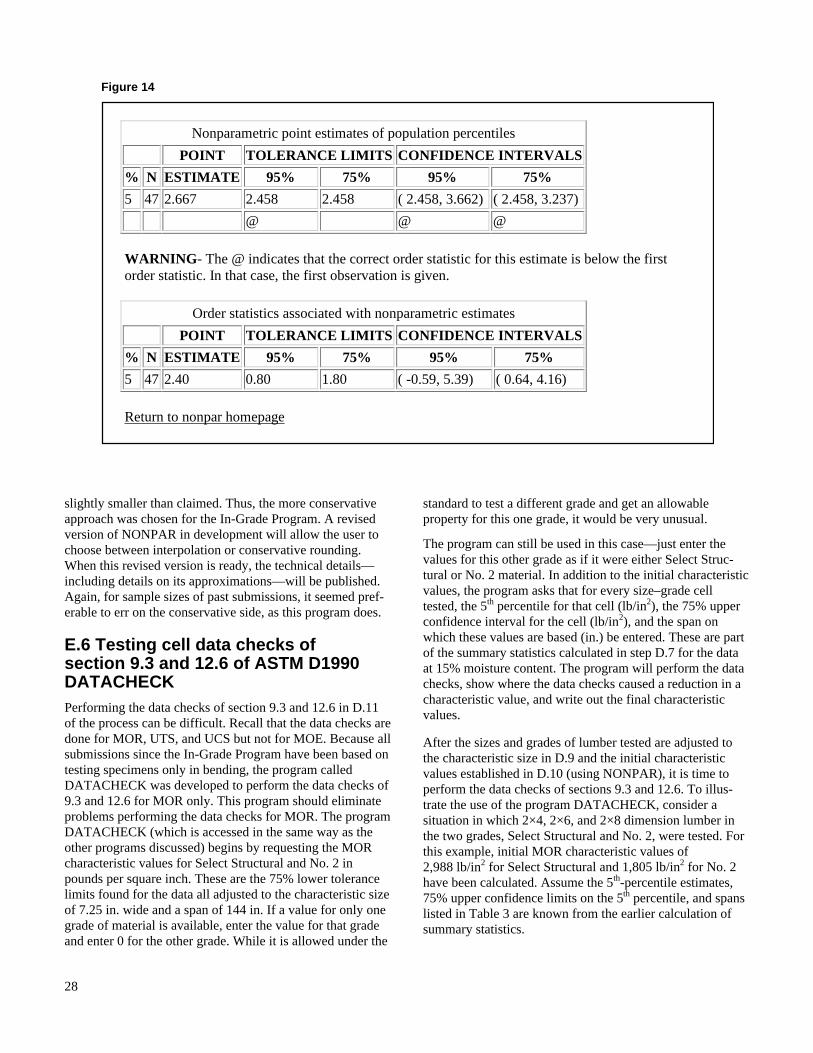
28

Figure 14

slightly smaller than claimed. Thus, the more conservative approach was chosen for the In-Grade Program. A revised version of NONPAR in development will allow the user to choose between interpolation or conservative rounding. When this revised version is ready, the technical details—including details on its approximations—will be published. Again, for sample sizes of past submissions, it seemed pref-erable to err on the conservative side, as this program does.

E.6 Testing cell data checks of section 9.3 and 12.6 of ASTM D1990 DATACHECK Performing the data checks of section 9.3 and 12.6 in D.11 of the process can be difficult. Recall that the data checks are done for MOR, UTS, and UCS but not for MOE. Because all submissions since the In-Grade Program have been based on testing specimens only in bending, the program called DATACHECK was developed to perform the data checks of 9.3 and 12.6 for MOR only. This program should eliminate problems performing the data checks for MOR. The program DATACHECK (which is accessed in the same way as the other programs discussed) begins by requesting the MOR characteristic values for Select Structural and No. 2 in pounds per square inch. These are the 75% lower tolerance limits found for the data all adjusted to the characteristic size of 7.25 in. wide and a span of 144 in. If a value for only one grade of material is available, enter the value for that grade and enter 0 for the other grade. While it is allowed under the

standard to test a different grade and get an allowable property for this one grade, it would be very unusual.

The program can still be used in this case—just enter the values for this other grade as if it were either Select Struc-tural or No. 2 material. In addition to the initial characteristic values, the program asks that for every size–grade cell tested, the 5th percentile for that cell (lb/in2), the 75% upper confidence interval for the cell (lb/in2), and the span on which these values are based (in.) be entered. These are part of the summary statistics calculated in step D.7 for the data at 15% moisture content. The program will perform the data checks, show where the data checks caused a reduction in a characteristic value, and write out the final characteristic values.

After the sizes and grades of lumber tested are adjusted to the characteristic size in D.9 and the initial characteristic values established in D.10 (using NONPAR), it is time to perform the data checks of sections 9.3 and 12.6. To illus-trate the use of the program DATACHECK, consider a situation in which 2×4, 2×6, and 2×8 dimension lumber in the two grades, Select Structural and No. 2, were tested. For this example, initial MOR characteristic values of 2,988 lb/in2 for Select Structural and 1,805 lb/in2 for No. 2 have been calculated. Assume the 5th-percentile estimates, 75% upper confidence limits on the 5th percentile, and spans listed in Table 3 are known from the earlier calculation of summary statistics.

Nonparametric point estimates of population percentiles

POINT TOLERANCE LIMITS CONFIDENCE INTERVALS

% N ESTIMATE 95% 75% 95% 75%

5 47 2.667 2.458 2.458 ( 2.458, 3.662) ( 2.458, 3.237)

@ @ @

WARNING - The @ indicates that the correct order statistic for this estimate is below the first order statistic. In that case, the first observation is given.

Order statistics associated with nonparametric estimates

POINT TOLERANCE LIMITS CONFIDENCE INTERVALS

% N ESTIMATE 95% 75% 95% 75%

5 47 2.40 0.80 1.80 ( -0.59, 5.39) ( 0.64, 4.16)

Return to nonpar homepage

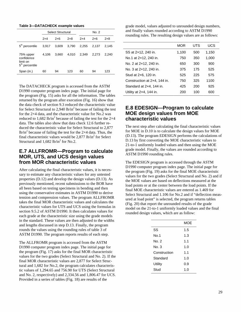
29

The DATACHECK program is accessed from the ASTM D1990 computer program index page. The initial page for the program (Fig. 15) asks for all the information. The tables returned by the program after execution (Fig. 16) show that the data check of section 9.3 reduced the characteristic value for Select Structural to 2,940 lb/in2 because of failing the test for the 2×4 data, and the characteristic value for No.2 was reduced to 1,682 lb/in2 because of failing the test for the 2×4 data. The tables also show that data check 12.6 further re-duced the characteristic value for Select Structural to 2,877 lb/in2 because of failing the test for the 2×4 data. Thus, the final characteristic values would be 2,877 lb/in2 for Select Structural and 1,682 lb/in2 for No.2.

E.7 ALLFROMR—Program to calculate MOR, UTS, and UCS design values from MOR characteristic values After calculating the final characteristic values, it is neces-sary to estimate any characteristic values for any untested properties (D.12) and develop the design values (D.13). As previously mentioned, recent submissions to the BOR have all been based on testing specimens in bending and then using the conservative estimates in ASTM D1990 to derive tension and compression values. The program ALLFROMR takes the final MOR characteristic values and calculates the characteristic values for UTS and UCS using the formulas in section 9.5.2 of ASTM D1990. It then calculates values for each grade at the characteristic size using the grade models in the standard. These values are then adjusted to the widths and lengths discussed in step D.13. Finally, the program rounds the values using the rounding rules of table 3 of ASTM D1990. The program reports results of each step.

The ALLFROMR program is accessed from the ASTM D1990 computer program index page. The initial page for the program (Fig. 17) asks for the final MOR characteristic values for the two grades (Select Structural and No. 2). If the final MOR characteristic values are 2,877 for Select Struc-tural and 1,682 for No.2, the program calculates characteris-tic values of 1,294.65 and 756.90 for UTS (Select Structural and No. 2, respectively) and 2,334.56 and 1,806.47 for UCS. Provided in a series of tables (Fig. 18) are results of the

grade model, values adjusted to unrounded design numbers, and finally values rounded according to ASTM D1990 rounding rules. The resulting design values are as follows:

MOR UTS UCS

SS at 2×12, 240 in. 1,100 500 1,150

No.1 at 2×12, 240 in. 750 350 1,000

No. 2 at 2×12, 240 in. 650 300 900

No. 3 at 2×12, 240 in. 375 175 525

Stud at 2×6, 120 in. 525 225 575

Construction at 2×4, 144 in. 750 325 1100

Standard at 2×4, 144 in. 425 200 925

Utility at 2×4, 144 in. 200 100 600

E.8 EDESIGN—Program to calculate MOE design values from MOE characteristic values The next step after calculating the final characteristic values for MOE in D.10 is to calculate the design values for MOE (D.13). The program EDESIGN performs the calculations of D.13 by first converting the MOE characteristic values to 21-to-1 uniformly loaded values and then using the MOE grade model. Finally, the values are rounded according to ASTM D1990 rounding rules.

The EDESIGN program is accessed through the ASTM D1990 computer program index page. The initial page for the program (Fig. 19) asks for the final MOE characteristic values for the two grades (Select Structural and No. 2) and if the MOE values are based on deflections measured at the load points or at the center between the load points. If the final MOE characteristic values are entered as 1.469 for Select Structural and 1.106 for No.2 and if “deflection meas-ured at load point” is selected, the program returns tables (Fig. 20) that report the unrounded results of the grade model on the 21-to-1 uniformly loaded values and the final rounded design values, which are as follow:

MOE

SS 1.5

No.1 1.3

No. 2 1.1

No. 3 1.0

Construction 1.1

Standard 1.0

Utility 0.9

Stud 1.0

Table 3—DATACHECK example values

Select Structural No. 2

2×4 2×6 2×8 2×4 2×6 2×8

5th percentile 3,917 3,609 3,790 2,255 2,137 2,145

75% upper confidence limit on 5th percentile

4,106 3,660 4,010 2,349 2,273 2,240

Span (in.) 60 94 123 60 94 123

30

Figure 15 (page 1 of 2)

WWW Computer Program for Testing Cell Data Checks of Section 9.3 and 12.6 of ASTM D1990

This program assumes that we have one or more sizes of specimens for both Select Structural and Number 2 grades of dimension lumber. We will deal with the Modulus of Rupture (MOR) characteristic.

Please enter your MOR Select Structural Characteristic value in psi 2988

Please enter your MOR No. 2 Characteristic value in psi 1805

Please input the estimated 5th percentile, the 75% upper confidence interval for the 5th percentile and the test span width for each cell that you have data. All values are assumed to be at 15% moisture content. These values are the summary statistics before adjusting to the charcteristic size.

• 2x4 Select Structural

o 3917

5th Percentile (psi)

o 4106

75th Upper Confidence Interval for 5th Percentile (psi)

o 60

Span Width, i.e. 60.4 (inches) • 2x6 Select Structural

o 3609

5th Percentile (psi)

o 3660

75th Upper Confidence Interval for 5th Percentile (psi)

o 94

Span Width, i.e. 60.4 (inches) • 2x8 Select Structural

o 3790

5th Percentile (psi)

o 4010

75th Upper Confidence Interval for 5th Percentile (psi)

o 123

Span Width, i.e. 60.4 (inches) • 2x10 Select Structural

o 5th Percentile (psi)

o 75th Upper Confidence Interval for 5th Percentile (psi)

o Span Width, i.e. 60.4 (inches) • 2x12 Select Structural

o 5th Percentile (psi)

o 75th Upper Confidence Interval for 5th Percentile (psi)

o Span Width, i.e. 60.4 (inches)

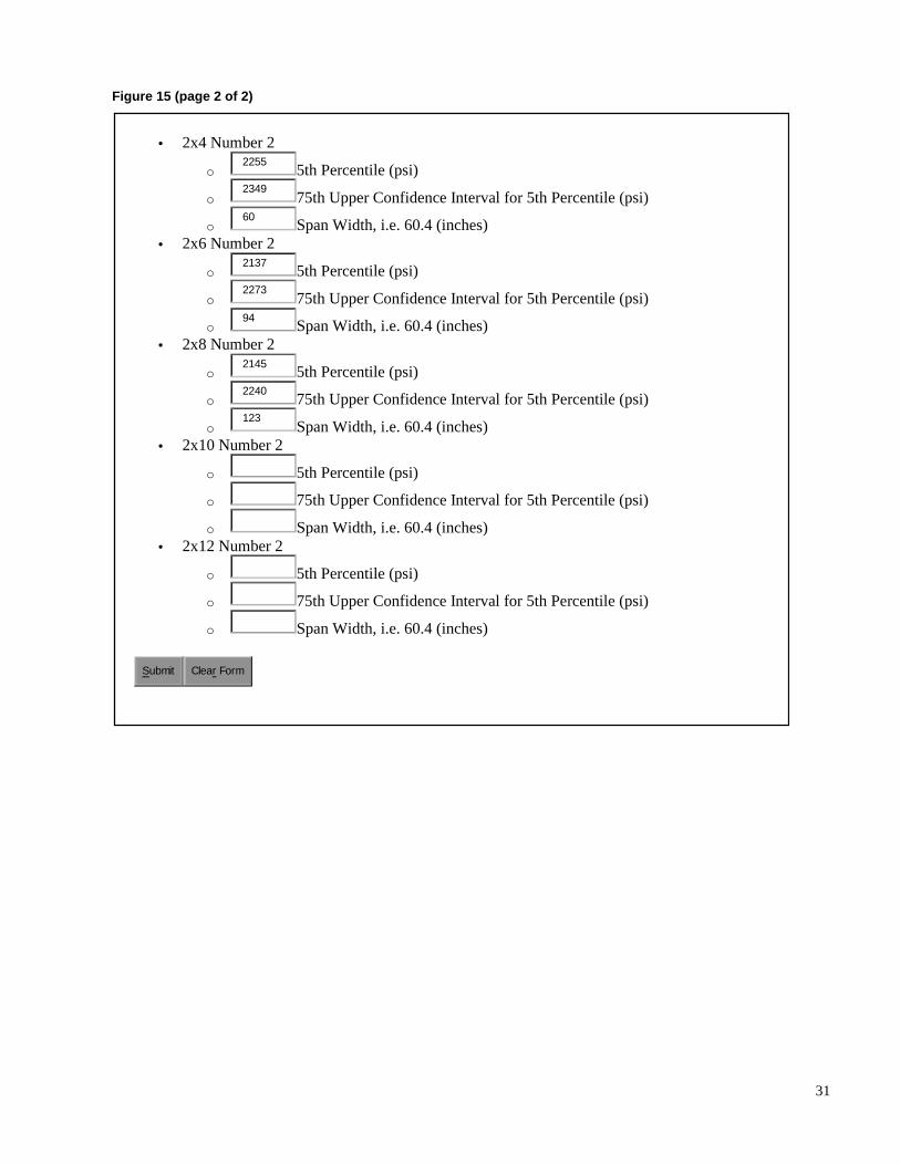
31

Figure 15 (page 2 of 2)

• 2x4 Number 2

o 2255

5th Percentile (psi)

o 2349

75th Upper Confidence Interval for 5th Percentile (psi)

o 60

Span Width, i.e. 60.4 (inches) • 2x6 Number 2

o 2137

5th Percentile (psi)

o 2273

75th Upper Confidence Interval for 5th Percentile (psi)

o 94

Span Width, i.e. 60.4 (inches) • 2x8 Number 2

o 2145

5th Percentile (psi)

o 2240

75th Upper Confidence Interval for 5th Percentile (psi)

o 123

Span Width, i.e. 60.4 (inches) • 2x10 Number 2

o 5th Percentile (psi)

o 75th Upper Confidence Interval for 5th Percentile (psi)

o Span Width, i.e. 60.4 (inches) • 2x12 Number 2

o 5th Percentile (psi)

o 75th Upper Confidence Interval for 5th Percentile (psi)

o Span Width, i.e. 60.4 (inches)

Submit Clear Form

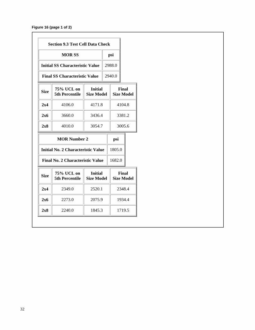
32

Figure 16 (page 1 of 2)

Section 9.3 Test Cell Data Check

MOR SS psi

Initial SS Characteristic Value 2988.0

Final SS Characteristic Value 2940.0

Size 75% UCL on 5th Percentile

Initial Size Model

Final Size Model

2x4 4106.0 4171.8 4104.8

2x6 3660.0 3436.4 3381.2

2x8 4010.0 3054.7 3005.6

MOR Number 2 psi

Initial No. 2 Characteristic Value 1805.0

Final No. 2 Characteristic Value 1682.0

Size 75% UCL on 5th Percentile

Initial Size Model

Final Size Model

2x4 2349.0 2520.1 2348.4

2x6 2273.0 2075.9 1934.4

2x8 2240.0 1845.3 1719.5

33

Figure 16 (page 2 of 2)

Section 12.6 Test Cell Data Check

MOR SS psi

Initial SS Characteristic Value 2940.0

Final SS Characteristic Value 2877.0

Size Cell +5% Cell +100 Initial Size Model

Final Size Model

2x4 4112.8 4017.0 4104.8 4016.9

2x6 3789.4 3709.0 3381.2 3308.8

2x8 3979.5 3890.0 3005.6 2941.2

MOR Number 2 psi

Initial No. 2 Characteristic Value 1682.0

Final No. 2 Characteristic Value 1682.0

Size Cell +5% Cell +100 Initial Size Model

Final Size Model

2x4 2367.8 2355.0 2348.4 2348.4

2x6 2243.8 2237.0 1934.4 1934.4

2x8 2252.2 2245.0 1719.5 1719.5

34

Figure 17

WWW Computer Program for Producing Unrounded and Rounded Design Values for

MOR, UTS, and UCS

This program takes ASTM D1990 characteristic values for MOR and produces unrounded and rounded design values for Modulus of Rupture (MOR), Ultimate Tensile Strength (UTS) and Ultimate Compression Strength (UCS). Property reduction factors for softwoods were used.

Please enter the MOR SS Characteristic value in psi 2877

Please enter the MOR No. 2 Characteristics value in psi 1682

Submit Clear Form

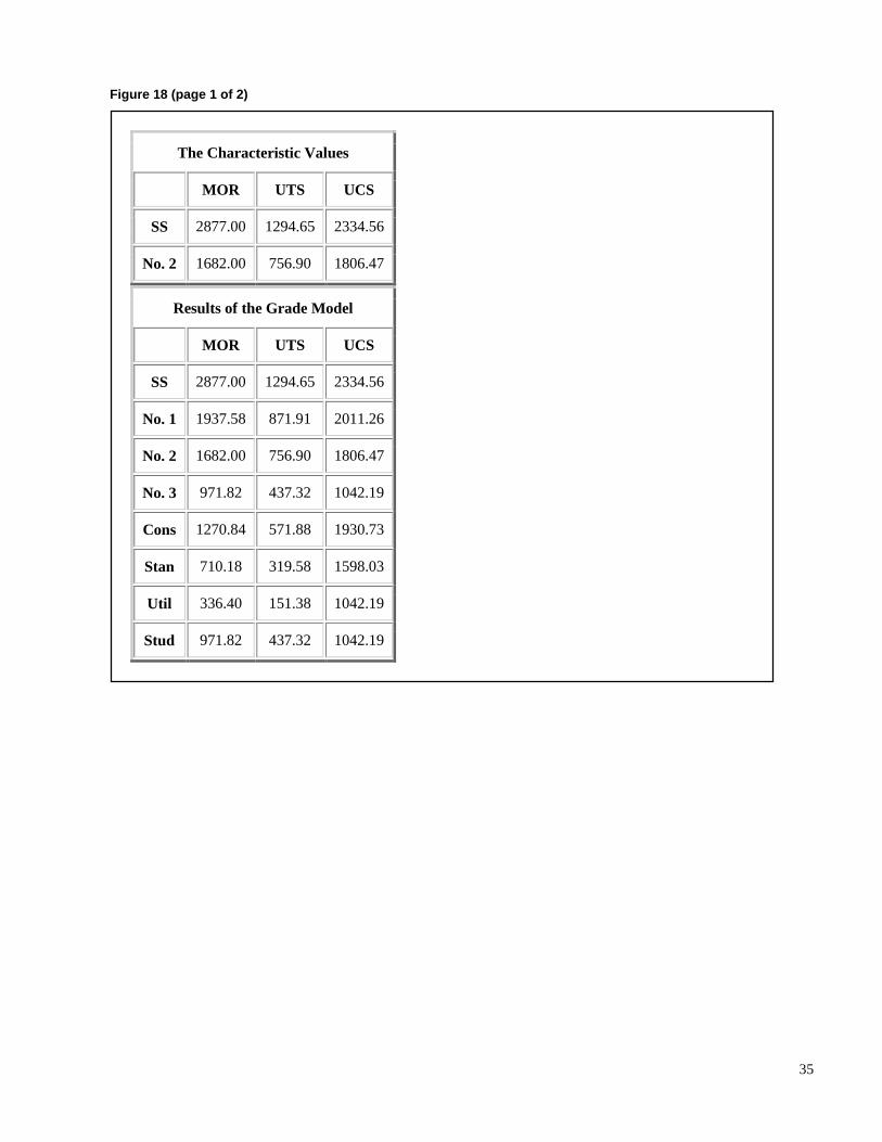
35

Figure 18 (page 1 of 2)

The Characteristic Values

MOR UTS UCS

SS 2877.00 1294.65 2334.56

No. 2 1682.00 756.90 1806.47

Results of the Grade Model

MOR UTS UCS

SS 2877.00 1294.65 2334.56

No. 1 1937.58 871.91 2011.26

No. 2 1682.00 756.90 1806.47

No. 3 971.82 437.32 1042.19

Cons 1270.84 571.88 1930.73

Stan 710.18 319.58 1598.03

Util 336.40 151.38 1042.19

Stud 971.82 437.32 1042.19

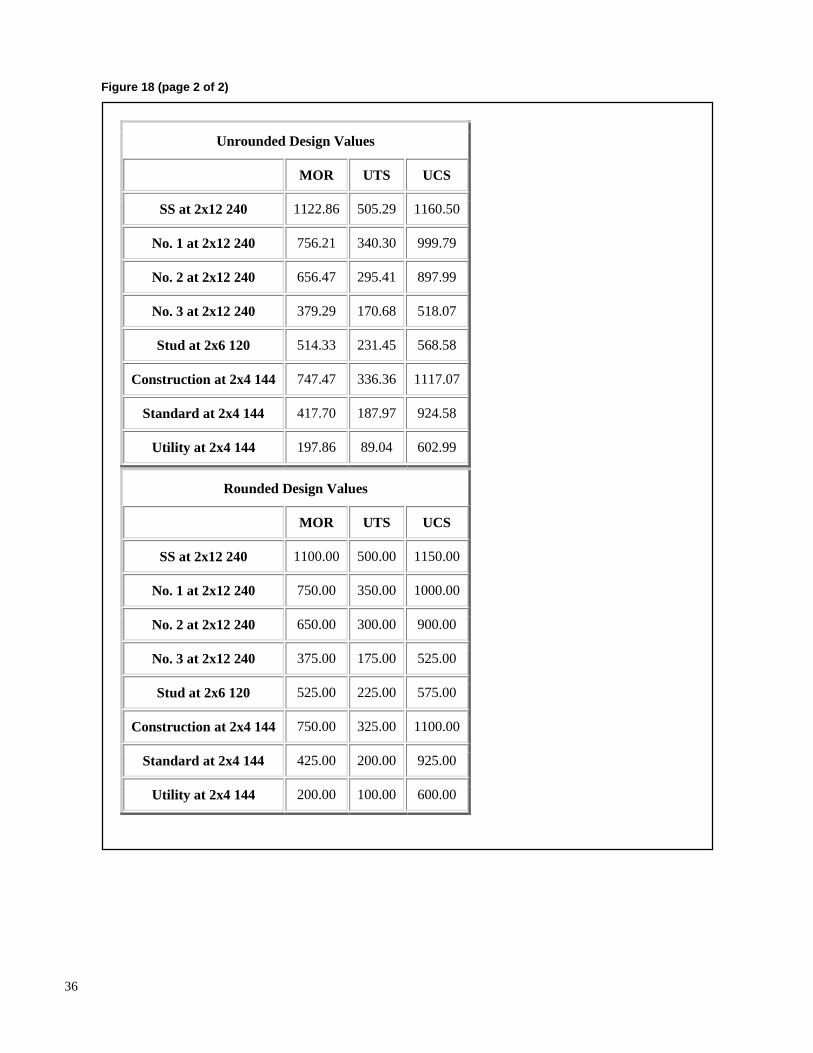
36

Figure 18 (page 2 of 2)

Unrounded Design Values

MOR UTS UCS

SS at 2x12 240 1122.86 505.29 1160.50

No. 1 at 2x12 240 756.21 340.30 999.79

No. 2 at 2x12 240 656.47 295.41 897.99

No. 3 at 2x12 240 379.29 170.68 518.07

Stud at 2x6 120 514.33 231.45 568.58

Construction at 2x4 144 747.47 336.36 1117.07

Standard at 2x4 144 417.70 187.97 924.58

Utility at 2x4 144 197.86 89.04 602.99

Rounded Design Values

MOR UTS UCS

SS at 2x12 240 1100.00 500.00 1150.00

No. 1 at 2x12 240 750.00 350.00 1000.00

No. 2 at 2x12 240 650.00 300.00 900.00

No. 3 at 2x12 240 375.00 175.00 525.00

Stud at 2x6 120 525.00 225.00 575.00

Construction at 2x4 144 750.00 325.00 1100.00

Standard at 2x4 144 425.00 200.00 925.00

Utility at 2x4 144 200.00 100.00 600.00

37

Figure 19

WWW Computer Program for Producing Unrounded Design Values For Modulus of

Elasticity (MOE)

This program takes ASTM D1990 characteristic values for MOE (at 17 to 1 and 3rd point loaded) with deflections measured at load point or midspan and produces unrounded design values for MOE at 21 to 1 uniformly loaded.

Where did you measure deflections?

� �� �� �

Deflection measured at load point � ��

Deflection measured at midspan

Please enter the SS value for MOE 17 to 1 value (million psi) 1.469

Please enter the No. 2 value for MOE at 17 to 1 (million psi) 1.106

Submit Clear Form

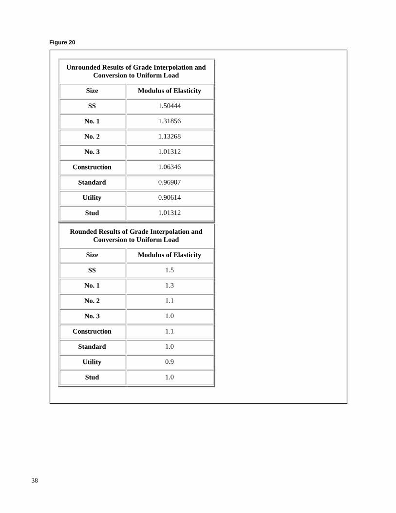
38

Figure 20

Unrounded Results of Grade Interpolation and Conversion to Uniform Load

Size Modulus of Elasticity

SS 1.50444

No. 1 1.31856

No. 2 1.13268

No. 3 1.01312

Construction 1.06346

Standard 0.96907

Utility 0.90614

Stud 1.01312

Rounded Results of Grade Interpolation and Conversion to Uniform Load

Size Modulus of Elasticity

SS 1.5

No. 1 1.3

No. 2 1.1

No. 3 1.0

Construction 1.1

Standard 1.0

Utility 0.9

Stud 1.0

39

F. Discussion and Summary This report is intended to explained and simplified the proc-ess of developing allowable properties under ASTM D1990. There is no one single way to obtain allowable properties. However, where multiple approaches have been used, we generally try to show the different approaches and indicate any differences.

We offer several recommendations for the better approach in some cases and for specific clarification of the standard:

• The standard should be modified to specify what to do when a species fails the grade quality index (GQI) test.

• The concept of a GQI test is vague in situations where several species are to be grouped—this should be ad-dressed in the standard.

• Data should be collected in a way that eliminates as many adjustments as possible. This includes using ov-endry moisture contents, testing at 73°F, and testing at 17-to-1 span-to-depth ratio using third point loading and measuring deflection at the load heads.

• The new temperature adjustment model for MOE should be used and incorporated in the standard.

• We recommend against normalization in adjustments of strength properties to different moisture contents.

• Anyone developing allowable properties under ASTM D1990 should perform many of the necessary calcula-tion using the series of computer programs developed by the Forest Products Laboratory and available on the World Wide Web.

G. References AF&PA. 1997. National design specification for wood construction. Washington DC: American Forest and Paper Association.

ASTM. 1998. Annual book of ASTM standards. Vol. 04.10 Wood. West Conshohocken, PA: American Society for Testing and Materials.

D245–93. Standard practice for establishing structural grades and related allowable properties for visually graded lumber: 75–92.

D2915–94. Standard practice for evaluating allowable properties for grades of structural lumber: 397–408.

D2555–96. Standard test methods for establishing clear wood strength values: 359–374.

D4761–96. Standard test methods for mechanical properties of lumber and wood-base structural material: 505–513.

D198–97. Standard test methods of static tests of lumber in structural sizes: 56–74.

D1990–97. Standard practice for establishing allowable properties for visually-graded dimension lumber from In-grade tests of full-size specimens: 287–311.

Anonymous. Operating instructions for Moore moisture meter model RC-1B.

Barrett, J.D.; Green, D.W.; Evans, J.W. 1989. Tempera-ture adjustments for the North American In-grade testing program. In: Green, D.W.; Shelley, B.E.; Vokey, H.P., eds. In-grade testing of structural lumber. Proceedings 47363. Madison, WI: Forest Products Society: 27–38.

Bramhall, G.; Salamon, M. 1978. Combined species-temperature correction tables for moisture meters. Inf. Rep. VPX–103 (rev.). Forestry Directorate, Environment Canada, WFPL.

Cech, M.Y.; Pfaff, F. 1975. Moisture content correction tables for resistance-type moisture meters. Rep. 7. Canadian Forest Service. Department of Environment.

Evans, J.W.; Green, D.W. 1988a. Mechanical properties of visually graded dimension lumber: Vol. 2 Douglas Fir–Larch. Pub. PB–88–159–397. Springfield, VA: National Technical Information Service. 476 p.

Evans, J.W.; Green, D.W. 1988b. Mechanical properties of visually graded dimension lumber: Vol. 3. Hem-Fir. Pub. PB–88–159–405. Springfield, VA: National Technical Information Service. 392 p.

Evans, J.W.; Green, D.W. 1988c. Mechanical properties of visually graded dimension lumber: Vol. 5. Aspen-Cottonwood, Balsam Fir, Douglas Fir (South). Pub. PB–88–159–421. Springfield, VA: National Technical Information Service. 510 p.

Evans, J.W.; Green, D.W. 1988d. Mechanical properties of visually graded dimension lumber: Vol. 8. Sitka Spruce, Subalpine Fir, Sugar Pine, Tamarack, Yellow-Poplar. Pub. PB–88–159–454. Springfield, VA: National Technical Information Service. 492 p.

Garrahan, P. 1989. Moisture meter correction factors. In: Green, D.W.; Shelley, B.E.; Vokey, H.P., eds. In-grade testing of structural lumber. Proceedings 47363. Madison, WI: Forest Products Society 39–43.

Green, D.W.; Evans, J.W. 1988a. Mechanical properties of visually graded dimension lumber: Vol. 1. A summary. Pub. PB–88–159–389. Springfield, VA: National Technical Information Service. 131 p.

Green, D.W.; Evans, J.W. 1988b. Mechanical properties of visually graded dimension lumber: Vol. 4. Southern Pine. Pub. PB–88–159–413. Springfield, VA: National Technical Information Service. 412 p.

40

Green, D.W.; Evans, J.W. 1988c. Mechanical properties of visually graded dimension lumber: Vol. 6. Eastern Hemlock, Eastern Spruces, Eastern White Pine, Engelmann Spruce, Idaho White Pine, Jack Pine. Pub. PB–88–159–439. Spring-field, VA: National Technical Information Service. 560 p.

Green, D.W.; Evans, J.W. 1988d. Mechanical properties of visually graded dimension lumber: Vol. 7. (Minor) Southern Pines, Ponderosa Pine, Red Pine. Pub. PB–88–159–447. Springfield, VA: National Technical Information Service. 542 p.

Green, D.W.; Evans, J.W. 1988e. Evaluating lumber prop-erties: practical concerns and theoretical restraints. In: Itani, Rafik Y., ed. Proceedings of the 1988 International confer-ence on timber engineering; 1988 September 19–22; Vol. 1: 203–217.

Green, D.W.; Evans, J.W. 1989. Moisture content and the mechanical properties of dimension lumber: decisions for the future. In: Green, D.W.; Shelley, B.E.; Vokey, H.P., eds. In-grade testing of structural lumber. Proceedings 47363. Madison, WI: Forest Products Society: 44–55.

Green, D.W.; Evans, J.W. 2001a. Temperature effects on the modulus of elasticity of very dry lumber. In preparation.

Green, D.W.; Evans, J.W. 2001b. Evolution of standard-ized procedures for adjusting lumber properties for changes in moisture content. Gen. Tech. Rep. Madison, WI: U.S. Department of Agriculture, Forest Service, Forest Products Laboratory.

Green, D.W.; Hernandez, R. 1998. Codes and standards for structural wood products and their use in the United States. In: Proceedings of the Forest Products Study Group Workshop; 1998, June 23; Mérida, Yucátan, México: 16 p.

Green, D.W.; Shelley, B.E; Vokey, H.P. (eds.) 1989. In-grade testing of structural lumber. Proceedings 47363. Madison, WI: Forest Products Society. 110 p.

Green, D.W.; Shelley, B.E. 1994. Establishing allowable design values for structural lumber of foreign species for use in the United States. In: The globalization of wood: supply, process, and markets. Proceedings of conference; 1993 November 1–3; Portland, OR. Proceedings 7319. Madison, WI: Forest Products Society: 215–228.

Green, D.W.; Evans, J.W.; Logan, J.D.; Nelson, W.J. 1999. Adjusting modulus of elasticity of lumber for changes in temperature. Forest Products Journal. 49(10): 82–94.

Jones, E. 1989. Sampling procedures used in the in-grade lumber testing program. In: Green, D.W.; Shelley, B.E.; Vokey, H.P., eds. In-grade testing of structural lumber. Proceedings 47363. Madison, WI: Forest Products Society: 11–14.

Pellerin, R.F.; Gerhards, C.C. 1980. In-Grade testing program evaluation of a portable machine for testing lumber in bending. Madison, WI: U.S. Department of Agriculture, Forest Service, Forest Products Laboratory.

Pfaff, F. 1974. Electric moisture meter correction factors for eastern Canadian species. Rep. OPX–89E. Eastern Forest Products Laboratory. Forest Service, Environment Canada.

Pfaff, F.; Garrahan, P. 1984. Temperature correlation factors and combined temperature-species correction factors for the resistance type moisture meter. Project. 03–40–10–001 (unpublished). Forintek Canada Corp., Eastern Lab.

Salamon. M. 1971. Resistance moisture meter correction factors for western softwood species. Forest Product Journal. 22(12): 46–47.

Shelley, B.E. 1989. Testing machines: development, calibra-tion, and comparative studies In: Green, D.W.; Shelley, B.E.; Vokey, H.P., eds. In-grade testing of structural lumber. Proceedings 47363. Madison, WI: Forest Products Society: 15–26.

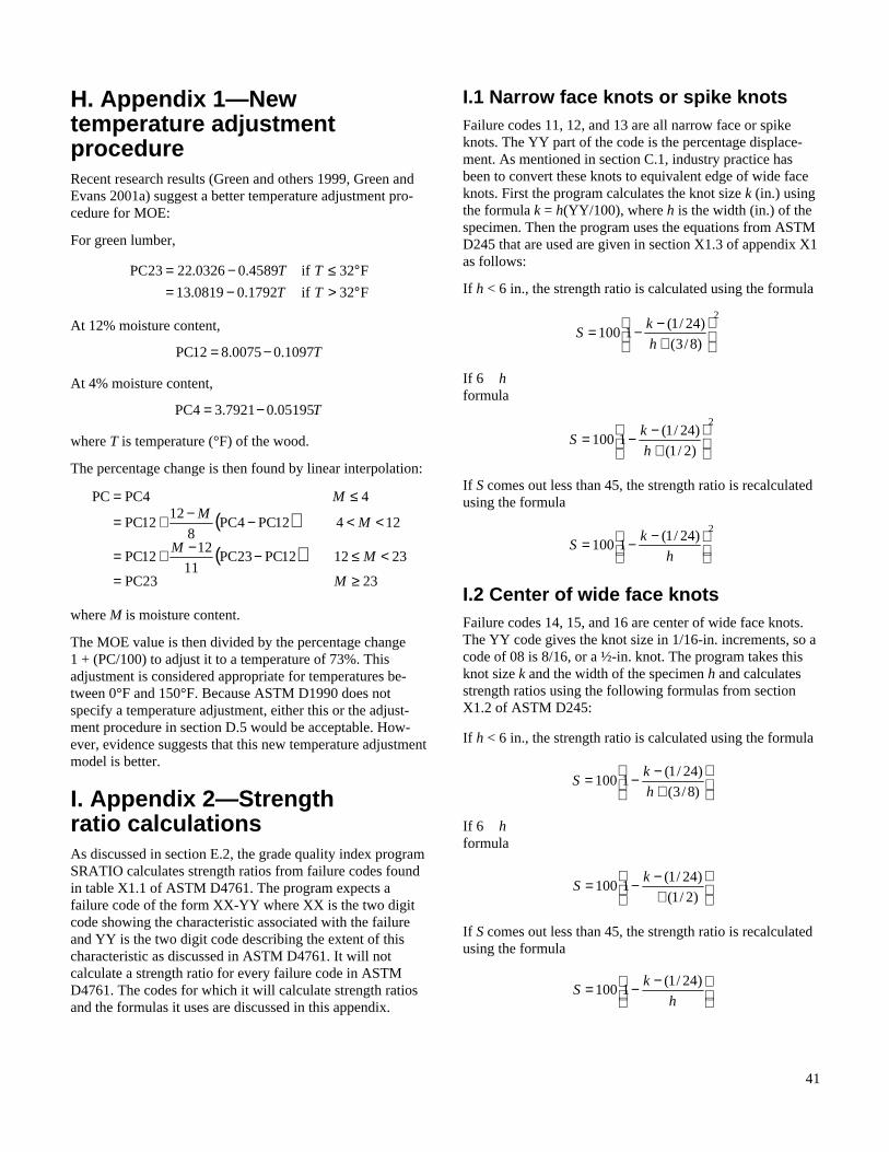
41

H. Appendix 1—New temperature adjustment procedure Recent research results (Green and others 1999, Green and Evans 2001a) suggest a better temperature adjustment pro-cedure for MOE:

For green lumber,

F32 if

F32 if

1792.00819.13

4589.00326.2223PC

°>°≤

−=−=

T

T

T

T

At 12% moisture content,

T1097.00075.812PC −=

At 4% moisture content,

T05195.07921.34PC −=

where T is temperature (°F) of the wood.

The percentage change is then found by linear interpolation:

( )

( )2323PC

231212PC23PC11

1212PC

12412PC4PC8

1212PC

44PCPC

≥=

<≤−−+=

<<−−+=

≤=

M

MM

MM

M

where M is moisture content.

The MOE value is then divided by the percentage change 1 + (PC/100) to adjust it to a temperature of 73%. This adjustment is considered appropriate for temperatures be-tween 0°F and 150°F. Because ASTM D1990 does not specify a temperature adjustment, either this or the adjust-ment procedure in section D.5 would be acceptable. How-ever, evidence suggests that this new temperature adjustment model is better.

I. Appendix 2—Strength ratio calculations As discussed in section E.2, the grade quality index program SRATIO calculates strength ratios from failure codes found in table X1.1 of ASTM D4761. The program expects a failure code of the form XX-YY where XX is the two digit code showing the characteristic associated with the failure and YY is the two digit code describing the extent of this characteristic as discussed in ASTM D4761. It will not calculate a strength ratio for every failure code in ASTM D4761. The codes for which it will calculate strength ratios and the formulas it uses are discussed in this appendix.

I.1 Narrow face knots or spike knots Failure codes 11, 12, and 13 are all narrow face or spike knots. The YY part of the code is the percentage displace-ment. As mentioned in section C.1, industry practice has been to convert these knots to equivalent edge of wide face knots. First the program calculates the knot size k (in.) using the formula k = h(YY/100), where h is the width (in.) of the specimen. Then the program uses the equations from ASTM D245 that are used are given in section X1.3 of appendix X1 as follows:

If h < 6 in., the strength ratio is calculated using the formula

2

)8/3(

)24/1(1100

+−−=

h

kS

If 6 h formula

2

)2/1(

)24/1(1100

+−−=

h

kS

If S comes out less than 45, the strength ratio is recalculated using the formula

2)24/1(

1100

−−=

h

kS

I.2 Center of wide face knots Failure codes 14, 15, and 16 are center of wide face knots. The YY code gives the knot size in 1/16-in. increments, so a code of 08 is 8/16, or a ½-in. knot. The program takes this knot size k and the width of the specimen h and calculates strength ratios using the following formulas from section X1.2 of ASTM D245:

If h < 6 in., the strength ratio is calculated using the formula

+−−=

)8/3(

)24/1(1100

h

kS

If 6 h formula

+−−=

)2/1(

)24/1(1100

kS

If S comes out less than 45, the strength ratio is recalculated using the formula

−−=

h

kS

)24/1(1100

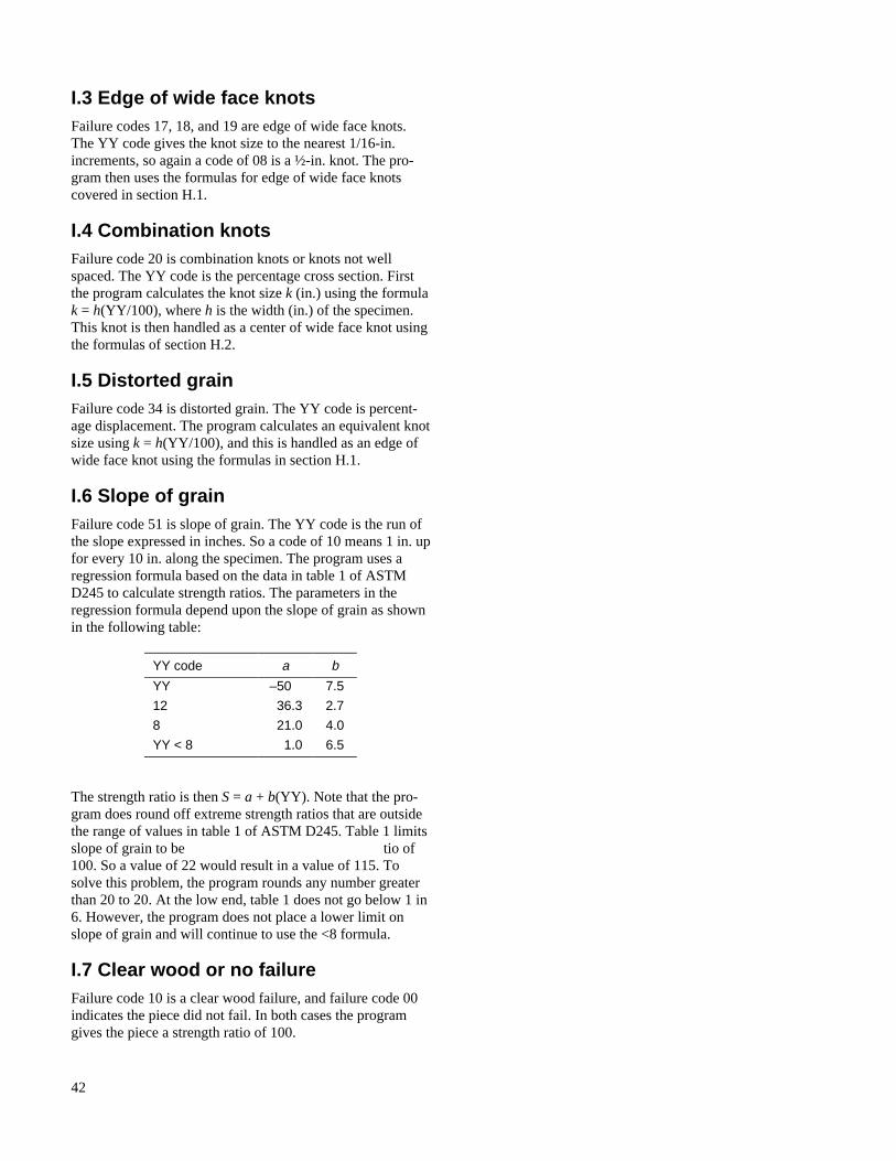
42

I.3 Edge of wide face knots Failure codes 17, 18, and 19 are edge of wide face knots. The YY code gives the knot size to the nearest 1/16-in. increments, so again a code of 08 is a ½-in. knot. The pro-gram then uses the formulas for edge of wide face knots covered in section H.1.

I.4 Combination knots Failure code 20 is combination knots or knots not well spaced. The YY code is the percentage cross section. First the program calculates the knot size k (in.) using the formula k = h(YY/100), where h is the width (in.) of the specimen. This knot is then handled as a center of wide face knot using the formulas of section H.2.

I.5 Distorted grain Failure code 34 is distorted grain. The YY code is percent-age displacement. The program calculates an equivalent knot size using k = h(YY/100), and this is handled as an edge of wide face knot using the formulas in section H.1.

I.6 Slope of grain Failure code 51 is slope of grain. The YY code is the run of the slope expressed in inches. So a code of 10 means 1 in. up for every 10 in. along the specimen. The program uses a regression formula based on the data in table 1 of ASTM D245 to calculate strength ratios. The parameters in the regression formula depend upon the slope of grain as shown in the following table:

YY code a b

YY –50 7.5

12 36.3 2.7

8 21.0 4.0

YY < 8 1.0 6.5

The strength ratio is then S = a + b(YY). Note that the pro-gram does round off extreme strength ratios that are outside the range of values in table 1 of ASTM D245. Table 1 limits slope of grain to be tio of 100. So a value of 22 would result in a value of 115. To solve this problem, the program rounds any number greater than 20 to 20. At the low end, table 1 does not go below 1 in 6. However, the program does not place a lower limit on slope of grain and will continue to use the <8 formula.

I.7 Clear wood or no failure Failure code 10 is a clear wood failure, and failure code 00 indicates the piece did not fail. In both cases the program gives the piece a strength ratio of 100.