Proc IMechE Part D: Modelling and optimal energy …mbahrami/pdf/2016/Modelling and optimal energy-saving... · shutdown period by considering different ... the model more complex

Original Article

Proc IMechE Part D:J Automobile Engineering1–19� IMechE 2016Reprints and permissions:sagepub.co.uk/journalsPermissions.navDOI: 10.1177/0954407016636978pid.sagepub.com

Modelling and optimal energy-savingcontrol of automotive air-conditioningand refrigeration systems

Yanjun Huang1, Amir Khajepour1, Farshid Bagheri2 and Majid Bahrami2

AbstractAir-conditioning and refrigeration systems are extensively adopted in homes, industry and vehicles. An important step inachieving a better performance and a higher energy efficiency for air-conditioning and refrigeration systems is a control-based model and a suitable control strategy. As a result, a dynamic model based on the moving-boundary and lumped-parameter method is developed in this paper. Unlike existing models, the proposed model lumps the effects of the finsinto two equivalent parameters without adding any complexity and considers the effect produced by the superheated sec-tion of the condenser, resulting in a model that is not only simpler but also more accurate than the existing models. Inaddition, a model predictive controller is designed on the basis of the proposed model to enhance the energy efficiency ofthe air-conditioning and refrigeration systems. Simulations and experimental results are presented to demonstrate theaccuracy of the model. The experiments show that an energy saving of about 8% can be achieved by using the proposedmodel predictive controller compared with the conventional on–off controller under the examined scenario. The betterperformance of the proposed controller requires electrification of the automotive air-conditioning and refrigeration sys-tems so as to eliminate the idling caused by running the air-conditioning and refrigeration systems when a vehicle stops.

KeywordsControl-based dynamic model, energy efficiency, model predictive controller, electrification of the automotive air-conditioning and refrigeration systems, idling

Date received: 4 November 2015; accepted: 26 January 2016

Introduction

The continuously increasing demands on lower emis-sion levels and better fuel economy have drivenresearchers to develop vehicles which are more efficientand less polluting.1 However, the main auxiliary loadof vehicles, the air-conditioning and refrigeration (A/C-R) systems, can consume up to 25% of the total fuel oreven more in long-haul service vehicles. In addition, asthe main energy consumption source in A/C-R systems,the compressor is usually connected directly to theengine via a belt in conventional vehicles, so thatengines sometimes have to idle in order to power theA/C-R systems during vehicle stops. For example,long-haul trucks are equipped with a sleeper cabinwhere the drivers can live when they are on the road.2

Usually, the trucks idle to provide power to the air-conditioning system for cabin temperature control.Similarly, food service trucks need to idle to providepower to the refrigeration system while loading orunloading. When the vehicle is idling, this gives rise to

many disadvatages, such as the low efficiency of theengine and excessive emissions.3 Thus, there are signifi-cant benefits in operating A/C-R systems efficiently, interms of both the operating costs and their effects onthe environment.4 An important step in achieving abetter performance and a higher energy efficiency is acontrol-based model and an appropriate control strat-egy.5 Therefore, making auxiliary devices more efficientcan result in many benefits to vehicle owners as well asto the environment. However, in most conventionalvehicles, the compressor speed is proportional to the

1Department of Mechanical and Mechatronics Engineering, University of

Waterloo, Waterloo, Ontario, Canada2School of Mechatronic System Engineering, Simon Fraser University,

Surrey, British Columbia, Canada

Corresponding author:

Yanjun Huang, Department of Mechanical and Mechatronics Engineering,

University of Waterloo, Waterloo, Ontario N2L3G1, Canada.

Email: [email protected]

by guest on April 27, 2016pid.sagepub.comDownloaded from

http://pid.sagepub.com/

engine speed instead of actively varying with therequirements of passengers or the working conditions.6

This impedes development of an advanced controllerfor automotive A/C-R systems given that the control-lers are usually applied to manipulate the speeds of thecompressor and the fans. However, in the developmentof anti-idling technologies such as auxiliary battery-powered units, hybrid electric vehicles (HEVs) and elec-tric vehicles (EV), the on-board energy storage systemis capable of powering the A/C-R systems indepen-dently so that the A/C-R systems can be disconnectedfrom the engines.7 This means that electrification of theA/C-R systems and thus application of an advancedcontroller in vehicles are possible.6 As a result, theidling caused by powering the auxiliary systems whenthe vehicle stops can be eliminated so that the perfor-mance and the efficiency of the automotive A/C-R sys-tems is greatly improved.8 This can be achievedpartially by developing advanced controllers to replacethe conventional on–off (bang–bang) controllers. Thedesign of advanced controllers requires a control-basedmodel of the A/C-R systems which is accurate but suf-ficiently simple for real-time implementation. Acontrol-based model is in fact a trade-off between theaccuracy and the simplicity. If the model is too simple,it is not be able to reflect the main characteristics of thesystem, which leads to a poor closed-loop control per-formance. On the other hand, if it is too complex, itslows down the controller by increasing the computa-tion time, which causes problems in real-time imple-mentations,9 although it can describe the dynamics ofthe system sufficiently well and produce good predic-tions. Consequently, this paper presents a simplifiedbut accurate model for A/C-R systems that was vali-dated by experimental results, and then the controllersare designed on the basis of the proposed model.

This paper is organized as follows: a literature reviewon the existing dynamic models of A/C-R systems ispresented in the second section; next, the moving-boundary lumped-parameter model is developed. Theparameters of the model are identified in the subsequentsection. Then, a brief introduction of the experimentalsystem as well as the simulations and experimentalresults are given for comparison and model validation.Furthermore, an on–off controller and a discrete modelpredictive controller are then developed, simulated,validated experimentally and compared in the next sec-tion. In the final section, comments and future work arediscussed.

Previous research

Overall, there are four main components in a vapourcompression cycle: the compressor, the evaporator, theexpansion valve and the condenser. The dynamics ofother auxiliary components such as the accumulatorand the receiver are incorporated into the connectingpipes or two heat exchangers. In the literature, the

modelling of the compressor valve and the expansionvalve, irrespective of their types (electric, thermostaticor automatic expansion valves), is demonstrated byalgebraic empirical equations.10 This is because thedynamics of a compressor valve and an expansion valveis an order of magnitude faster than those of the heatexchangers (the evaporator and the condenser).11

Several types of model have been constructed forheat exchangers for different purposes. For example,discretized or finite difference models are more accu-rate and are usually used in many commercial softwarepackages. These types of model can result in increasedaccuracy in prediction;12 however, they are too compli-cated to be used in the development and implementa-tion of a real-time control strategy. Another type ofheat exchanger model is based on lumped parametersand is usually a first-order time-invariant dynamicmodel; however, it has oversimplified most of thedynamic characteristics of heat exchangers.13 Aboveall, the most popular modelling approach is themoving-boundary (or moving-interface) lumped-parameter method, which is capable of reproducing thedynamics of multiple fluid-phase heat exchangers whilekeeping the simplicity of lumped-parameter models.13

Wedekind et al.14 contributed significantly by simplify-ing a class of two-phase transient flow problems into atype of lumped-parameter system. With experimentalconfirmation, they showed that the mean void fraction,i.e. the ratio of the vapour volume to the total fluid vol-ume of the two-phase region in a heat exchanger,remains relatively unchanged. This suggests that itstays constant, irrespective of how the refrigerant is dis-tributed throughout the heat exchanger and how thelength of the two-phase region changes.11 With thisassumption, this method allows the two-phase sectionto be modelled using lumped parameters. In this way,the whole model can be much more simplified than thediscretized model is. On the other hand, based on thefirst law of thermodynamics, the dynamics of the lengthof the two-phase section (the movement of the interfacebetween different regions) can be determined.

He11 used the moving-interface lumped-parametermodelling method. Based on several assumptions (e.g.that the heat exchanger is a long, thin and horizontaltube), He developed the complete non-linear dynamicmodel for the evaporator and the condenser, with morethan five states for each of them, and then derived theentire system model by considering the boundary con-ditions of all the components. However, in his research,only the linearized model was partially verified.

In recent years, Alleyne and co-workers haveimproved the model derived by He. For instance, Li15

constructed a model for the start-up period and theshutdown period by considering different distributionsof the refrigerant inside the heat exchangers.Rasmussen and Alleyne13 modelled the auxiliary com-ponents such as the accumulator and the receiver.Parameter identification algorithms for A/C-R systemmodelling have also been improved by Eldredge and

2 Proc IMechE Part D: J Automobile Engineering



Alleyne.16 Also, some special architectures for a vapourcompression cycle system were modelled by Fasl.17

Furthermore, the models were validated experimen-tally18–20 and showed overall improvements withrespect to the previous models. More importantly,McKinley and Alleyne21 considered the effects of thefins by introducing several other parameters such asthe ‘‘fraction of refrigerant-to-structure surface area onfins and refrigerant-side fin efficiency’’, which makesthe model more complex with nine states in the eva-porator alone. In all the models above, there are morethan 10 states representing the complexity of the model,which makes it difficult to guarantee the real-time run-ning of controllers developed on the basis of thesemodels. That is why He et al.22 developed a simplemodel of the whole system by assuming the identicaltemperature of the heat exchanger wall and reduced thenumber of states to five. In addition, a gain-schedulinglinear quadratic Gaussian technique was developed byusing this simplified model. Unfortunately, the simpli-fied model was not validated experimentally.

The disadvantages of the models existing in the liter-ature are as follows. First, the complete models withmore than 10 states are too complex to be used todevelop controllers. Second, the simple model doesinclude the effects of the fins when modelling heatexchangers, which results in discrepancies in the model.As a result, this paper is intended to improve furtherthe accuracy of the model reported by McKinley andAlleyne21 by incorporating the fins in the model of theheat exchangers in a new way without adding to thecomplexity of the model. The proposed model is vali-dated experimentally and compared with the existingmodel.

In this paper, an advanced model predictive control-ler is designed for the A/C-R systems for HEVs, EVsand conventional vehicles with auxiliary battery-powered units, where the A/C-R systems can be directlypowered by the on-board energy storage system. First,a simplified control-oriented dynamic model of theautomotive A/C-R systems is developed, where only sixstates instead of more than 10 states as reported in theliterature are used. In order to keep the accuracy of thissimplified model comparable with those of high-ordermodels, the effects of the fins are considered andlumped into two equivalent parameters. In addition,the effect of the superheated section of the condenser isalso included in the model by studying the experimentaldata instead of the model used by McKinley andAlleyne.21 This model is simulated and experimentallyvalidated for several scenarios. The results show thatthis model is simple and sufficiently accurate to be usedin real-time control systems. Using this model, anenergy-saving model predictive controller is designed,and its performance is compared with that of the con-ventional on–off controller. Because of some discreteconstraints, this model predictive controller is designedas a discrete model predictive controller, which is sel-dom mentioned in the existing literature. In addition,

since operation of the A/C-R systems increases the fuelconsumption by 90% at the maximum during vehicleidling,23 this work is an important step in developinganti-idling technologies for conventional vehicles. Forexample, the better performance and the higher energyefficiency of the proposed model predictive controllercan require electrification of the automotive A/C-R sys-tems so as to reduce vehicle idling. Furthermore, thisfast and robust model predictive controller can alwaysguarantee the minimum power consumption for A/C-Rsystems under any working conditions. Because of therelatively slow dynamics of the working conditions ofA/C-R systems, this slowly changing power consump-tion information can be integrated into a power man-agement strategy as the auxiliary power taken out ofthe energy storage system24 for prediction of the stateof charge to enhance the overall efficiency of the HEVsand EVs.

Model

An A/C-R system cycle or a vapour compression cyclegenerally consists of four main components, as shownin Figure 1, where the evaporator and condenser aredivided into several sections under normal workingconditions. There are two sections (i.e. the two-phasesection and the superheated section) in the evaporatorand three sections (i.e. the superheated section, the two-phase section and the subcooling section) in the con-denser. The valve is used to maintain the pressures ofthe two heat exchangers, while the compressor sendsthe refrigerant from the low-pressure heat exchanger tothe high-pressure heat exchanger.

The working principle of the A/C-R systems isbriefly described below. The refrigerant before enteringthe evaporator is characterized by the low-pressurelow-temperature two-phase state. In the evaporator, itabsorbs heat from the specific space and changes intothe vapour phase after exiting from the evaporator.The vapour refrigerant is compressed by the

Figure 1. Schematic diagram of the A/C-R systems.

Huang et al. 3



compressor and turned into high-pressure high-tem-perature vapour. It is then sent to the condenser wherethe removal of its heat results in a high-pressure low-temperature liquid phase. Finally, after going throughthe expansion valve, the pressure drops to the evapora-tor pressure, and the liquid refrigerant is changed intothe two-phase state. The same cycle is repeated again.

As is well known, the dynamics of the valve and thecompressor are so fast with respect to the cooling pro-cess that they can be treated by some empirical equa-tions obtained from test data. However, for the twoheat exchangers (the evaporator and the condenser),owing to their complex nature, the moving-boundarylumped-parameter modelling method is employed todevelop their control-based dynamic model.

In the vapour compression system modelled andexperimentally validated in this work, the expansionvalve is a thermostatic expansion valve, which adjustsits degree of opening according to the refrigerant tem-perature (the superheat temperature) at the outlet ofthe evaporator. The evaporator is a fin–tube type, andthe condenser is a microchannel type, as shown inFigure 2 and Figure 3 respectively. The refrigerant usedis R134a.25 This section presents only the main dynamicequations. For the complete version of the non-linearand linearized model for development of the model pre-dictive controller, see Appendix 2.

Thermostatic expansion valve

The expansion valve is assumed to be isenthalpic, i.e.the enthalpy at the valve inlet is identical with that atthe valve outlet.16 The other important parameter is therefrigerant mass flow rate _mv through the expansionvalve which is modelled by

_mv =CvAv

ffiffiffiffiffiffiffiffiffiffiffiffiffiffiffiffiffiffiffiffiffiffiffiffirv Pc � Peð Þ

pð1Þ

where Pc is the pressure of the condenser, Pe is the pres-sure of the evaporator, rv is the density of the refriger-ant at the valve inlet, Cv is the discharge coefficient(which is mapped as a polynomial correlation (Cv =fC(Pc– Pe)) of the pressure difference between the eva-porator and the condenser) and Av is the area of thevalve opening ( which is mapped as a polynomial corre-lation (Av = fA(Psat– Pe)) of the pressure differencebetween the evaporator and the saturation pressure ofthe evaporator outlet temperature). These correlationscan be obtained from experimental data. The remain-ing parameters such as the density can be obtainedfrom the thermodynamic properties25 of the refrigerantwhich have been compiled in look-up tables.

Compressor model

The dynamics of the compressor can be described by

_mcomp =NcompVdhvolrref Peð Þ ð2Þ

hoc =ha his Pe,Pcð Þ � hic Peð Þ½ �+ hic Peð Þ ð3Þ

where _mcomp is the refrigerant mass flow rate throughthe compressor, Ncomp is the compressor speed, Vd isthe volumetric displacement of the compressor, rref isthe density of the refrigerant inside the compressor, hocis the enthalpy at the compressor outlete, hic is theenthalpy at the compressor inlet, his(Pe, Pc) is the isen-tropic enthalpy during the compression process, whichcan be found from the thermodynamic properties ofthe refrigerant, hvol is the volumetric efficiency (whichcan be obtained from the polynomial correlation hvol

= fvol(Ncomp, Pc– Pe) with respect to the speed of com-pressor and the two pressures) and ha is the adiabaticefficiency (which can be obtained from the polynomialcorrelations ha = fa(Ncomp, Pc– Pe) with respect to thespeed of compressor and the two pressures).13,16,26

Fin–tube-type evaporator

Basically, two common types of heat exchanger areused in A/C-R systems: the fin–tube type and themicrochannel type. In the experimental system in thisstudy, the fin–tube-type evaporator as seen in Figure 2is used.

Under normal working conditions, the evaporatorcan be divided into two sections: the two-phase sectionand the superheated section. The modelling is based onthe whole heat transfer process: the heat convectionbetween the refrigerant inside the evaporator tube andthe tube wall and fins, the heat conduction throughoutthe tube wall and fins, and the heat convection betweenthe tube wall and fins and the ambient fluid-like air.This process is applied to the two sections. Based onthe energy conservation of the heat transfer processand the mean void fraction concept mentioned in theprevious section, the dynamic equations for each sec-tion can be obtained. Furthermore, the whole heat

Figure 2. Fin–tube type evaporator with plate fins.

Figure 3. Microchannel type condenser with louvre fins.




exchanger model can be developed by considering theboundary conditions between different sections.9,10

All the heat exchanger models in the literature arebased on the assumption of a long thin one-dimensionaltube. They do not consider the effects of the fins or con-sider them in a complicated way18 when modelling theheat convection between the tube wall and the refriger-ant inside. However, from Figure 2 and Figure 3, it canbe seen that there are many fins (plate type or louvreshape type) around the tube walls. Usually the fins andthe tubes are made from the same material. If the heatconduction throughout the fins is not considered, thisintroduces inaccuracy into the model.

Unlike the thin tube wall where no temperature gra-dient is assumed, the fins are long, and a one-dimensional temperature gradient exists along thelength of the fins. This gradient is dependent on thestructure of the fins and is difficult to simulate.However, from the perspective of energy conservation,the energy transferred from the refrigerant to the tubewall and fins is identical with the energy taken away bythe air and the energy kept in the wall and fins becuaseof their thermal inertia. In this way, the wall and thefins can be lumped together, as shown in the dashedrectangle in Figure 4. Thus, it is reasonable to utilize anequivalent temperature Twfe to represent the tempera-ture of the wall and the fins. The other equivalent para-meter used is the refrigerant-side heat transfercoefficient. In the evaporator, aie and aiesh are the coef-ficient for the two-phase section and the coefficient forthe superheated section respectively. After applyingthese equivalent parameters, the simplified non-lineardynamic model of the evaporator can be written as11,22

hlgerle 1� �geð ÞAedledt

= _mv hge � hie� �

� aiepDiele Twfe � Tre

� � ð4Þ

AeLe

drge

dPe

dPe

dt= _mv

hie � hlehlge

� _mcomp

+aiepDiele Twfe � Tre

� �hlge

ð5Þ

Cpm� �

wfe

dTwfe

dt=aoeAoe Tae � Twfe

� �� aiepDiele Twfe � Tre

� �� aieshpDie(Le � le) Twfe � Tre

� � ð6Þ

where the three states refer to the length le of the two-phase section, the pressure Pe of the evaporator andthe equivalent temperature Twfe of the tube wall andthe fins. Equation (4) simulates the energy transferfrom the refrigerant to the heat exchanger tube walland the fins of the two-phase section. The first term onthe right-hand side of this equation shows the energychange after the refrigerant goes through the two-phasesection, where hge is the enthalpy of the vapour refriger-ant under the current pressure, or the enthalpy at theboundary of the two sections, and hie is the enthalpy ofthe refrigerant at the evaporator inlet. The second termdescribes the energy absorbed from the evaporator tubewall and the fins of the two-phase section, where Die isthe inner diameter of the tube and Tre is the saturationtemperature of the refrigerant under the current pres-sure. Thus, the difference between these two terms rep-resents the energy absorbed or rejected by the two-phase section or the energy needed to evaporate theliquid refrigerant in the two-phase section. From thisenergy change, the two-phase length change can beobtained by using the left-hand side term, where hlge isthe latent enthalpy, rle is the liquid refrigerant density,1� �ge is the liquid volumetric fraction of the two-phasesection and Ae is the sectional area of the tube.18 Allthe enthalpies hge, hie and hlge, the densities rle, rge andrie, the density variation drge/dPe with respect to thepressure and the temperature Tre of the refrigerant canbe obtained from the thermodynamic properties25 ofthe used refrigerant which have been compiled in look-up tables; the heat transfer coefficients are identified byexperimental data and shown in Table 1.

Equation (5) denotes the vapour refrigerant changerate throughout the evaporator tube. The first term onthe right-hand side of this equation refers to the vapourmass at the evaporator inlet. As is known, the refriger-ant becomes a two-phase refrigerant after going

Figure 4. Schematic diagram of the evaporator with the equivalent parameters.

Huang et al. 5



through the expansion valve liquid. Based on theenthalpy hie of the refrigerant, the liquid enthalpy hleand the latent enthalpy hlge, the liquid percentage at theevaporator inlet can be found. The second term repre-sents the mass flow rate leaving the evaporator, whereasthe third term represents the vapour refrigerant whichhas changed from liquid. The left-hand side is thevapour mass change rate inside the evaporator. Thepressure change rate can be found via the densitychange rate by using the chain rule, where Le is the totallength of the evaporator tube wall and rge is the densityof the vapour refrigerant under the current evaporatorpressure Pe.

Equation (6) reflects the heat conduction of thewhole heat transfer process. The first term on the right-hand side refers to the total energy transferred to thetube wall and the fins from the ambient air, where aoe

is the heat transfer coefficient, which can be foundfrom the Colburn j-factor correlation, Aoe is the totaloutside area of the tube wall as well as the fins and Tae

is the mean air temperature. The last two terms are theenergy transferred from the tube wall and the fins tothe refrigerant in the two-phase section and the super-heated section respectively, where aiesh is the heat trans-fer coefficient in the superheated section. The left-handside shows the change in the temperature of the tubewall and the fins, where m is the total mass of the tubewall and the fins and Cp is the specific heat of the tubewall and the fins.

Since the equivalent temperature of the wall and thefins is defined on the basis of energy conservation, it isnot the temperature of the wall or the fins, and so itcannot be measured directly. After lumping the finsand the wall together, the Pierre correlation11 for calcu-lating the refrigerant-side heat transfer coefficient is nolonger suitable. However, these equivalent parameterscan be identified easily from equations (5) and (6).

Microchannel-type condenser

As mentioned above, the microchannel-type condenseris modelled and used in the experimental work. It canbe seen from Figure 3 that there are many louvre-shaped fins around each tube. There are many parallel

microchannels inside each tube. Under normal workingconditions, the refrigerant distribution is more complexthan that of the evaporator.

The condenser can be divided into three sections;however, in order to simplify the model for the purposeof real-time application, study of the experimental datasuggests that the subcooling section could be neglectedbecause of the much lower subcooling temperature(about 2 �C) compared with the superheat temperature(about 50 �C). Another reason is that the energyrejected to generate this lower subcooling temperatureis also relatively small. Also, the small energy errorcaused can be compensated by the equivalent heattransfer coefficient of the two-phase section. To makeup for this subcooling section from a temperature view-point, the refrigerant temperature at the condenser out-let can be found from experimental data. Using theabove assumptions, the condenser equations can beobtained in a similar manner to the evaporatorequations.

It is known that the total mass mtotal of the refriger-ant inside the cycle is constant without considering theleakage. The mass of refrigerant outside the two heatexchangers is defined as mpipe. Therefore, the differencebetween these two masses represents the mass inside theevaporator and the condenser, which can be obtainedfrom13

mtotal �mpipe =Ae rlele 1� �geð Þ+ rgele�ge + rshe Le � leð Þ� �

+Ac rlclc 1� �gcð Þ+ rgclc�gc + rshc Lc � lcð Þ� �

ð7Þ

The first term on the right-hand side refers to the refrig-erant mass of both the vapour and the liquid inside theevaporator, and the second term to that inside the con-denser, where lc is the length of the two-phase sectionof the condenser and �gc is the mean void fraction of thetwo-phase section of the condenser. Therefore, fromequations (4) and (7), the two-phase length of conden-ser can be found. As a result, there are only two states,namely the pressure Pc and the equivalent temperatureTwfc, which can be used to write the condenser equa-tions similar to the the evaporator equations22 accord-ing to

AcLc

drgc

dPc

dPc

dt= _mcomp �

aicpDiclc Trc � Twfc

� �hlgc

ð8Þ

Cpm� �

wfc

dTwfc

dt=aoc Ncondð ÞAoc Tac � Twfc

� �� aicpDiclc Twfc � Trc

� �� aicshpDic(Lc � lc)

Twfc �Trc +Tic

2

� � ð9Þ

The meanings and acquisition methods of all the para-meters used in the above equations are similar to thoseutilized in the explanations of equation (5) and equa-tion (6).

Table 1. The known and identified parameters at one steadystate.

Known parameter(units)

Value Identifiedparameter (units)

Value

Ncomp (r/min) 4500 le (m) 2.0137Nevap (Hz) 41.3 lc (m) 0.2528Ncond (Hz) 52.5 Twfe (�C) 3.84Te_air_in (�C) 20 Twfc (�C) 33.9Tc_air_in (�C) 27 aie (kW/m2 K) 0.68Pe (bar) 2.23 aic (kW/m2 K) 1.9Pc (bar) 8.95 aiesh (kW/m2 K) 0.045Tsh (�C) 2.74 aicsh (kW/m2 K) 0.13




Pipes

In the vapour compression cycle, the four main compo-nents are connected by several pipes of different sizes.Usually, the pipes are assumed to be adiabatic, and thepressure loss is neglected because of the short length.The refrigerant mass inside the pipe is mpipe, and it isestimated from the length and the inner diameter ofeach piece of pipe. Using the pressure inside the pipe,the density is found. The state of the refrigerant in eachpipe is assumed to be uniform except for the pipebetween the expansion valve and the evaporator, wherethe refrigerant is in the two-phase state. The vapourpercentage can be approximated by (hie– hle)/hlge, asexplained in the evaporator model.

Parameter estimation

In the vapour compression cycle model, there are threekinds of parameter: physical parameters, empiricalparameters and identified parameters.

Physical parameters

The physical parameters such as the dimensions of thepipes, the lengths, the inner and outer diameters andthe interior and exterior areas of the heat exchangerscan be easily measured or obtained from themanufacturers.

Empirical parameters

Empirical parameters can be estimated by empiricalequations obtained from the experimental data. Mostof these parameters vary with the working conditions.Therefore, each parameter should be calculated onlineto update its value. For each parameter, several corre-lations may exist. In the following section, the meanvoid fraction and the air-side heat transfer coefficientare be discussed in more detail.

The mean void fraction �g. The mean void fraction �g isdefined as the ratio of the vapour volume to the totalvolume in the two-phase region and has been employedto describe the characteristics of the two-phase flows.16

Wedekind et al.14 mentioned that the mean void frac-tion can be assumed to be constant during transientprocesses. However, recently this parameter has beenassumed to change with the fluid quality; it is definedas the ratio of the vapour mass to the total mass enter-ing the heat exchangers and is calculated from15,19

�g =1

b+

1

x2 � x1

a

bln

bx1 +a

bx2 +a

� � ð10Þ

with

a=rg

rf

S, b=1� a

where S is the slip ratio defined as the ratio of thevapour velocity to the liquid velocity in the two-phasesections and is identified by test data, x1 is the fluidquality at the inlet of the two-phase section and x2 isthe fluid quality at the outlet of the two-phase section.

Air-side heat transfer coefficient ao. The air-side heat trans-fer coefficient is related to the energy transferred fromthe heat exchanger tube wall and fins. However, for dif-ferent kinds of fin, there are different empirical correla-tions. In this study, the Colburn j factor is used, whichprovides a way of relating the Reynolds number of airflow through a heat exchanger to the experimentallydetermined heat transfer characteristics of the heatexchanger.13,17 The air-side heat transfer coefficient canbe found from the j factor by using

j=St Pr2=3 ð11Þ

where the Colburn j factor is related to the Reynoldsnumber and the physical structure of the heat exchan-ger. For the fin–tube-type evaporator, see the paper byNejad et al.27 and, for the microchannel condenser, seethe paper by Jabardo and Mamani.28 The Prandtl num-ber Pr is calculated at air temperature; the Stantonnumber13 St is related to the air-side heat transfer coef-ficient and is defined by

St=ao

GCpð12Þ

where G is the air mass flux across the heat exchangerand Cp is the thermal conductivity of air at the air tem-perature. By reconstructing the above two equations,the heat transfer coefficient becomes

ao =jGCp

Pr2=3ð13Þ

Mean air temperature Ta around the heat exchangers. Thisparameter can be assumed to be the mean temperatureof the air temperature at the inlet and the outlet of theheat exchanger.13 Taking the evaporator as an example,in order to find the air temperature at the outlet of theheat exchanger, Tae should first be calculated from

Tae=

2_mair eCp, air

aoeAoe

� �Ta, in+Twfe

�2

_mair eCp, air

aoeAoe

� �+1

ð14Þ

where _mair e is the air mass flow rate going through theevaporator and Cp,air is the specific heat of the air. Inthis process, _mair e is proportional to the control signalNevap of the evaporator fan. This proportional coeffi-cient can be identified by using experimental data. Tac

at the condenser side can be calculated in a similar man-ner. Ta,in is the air temperature at the evaporator inletand is measured by thermocouples.

Huang et al. 7



Identified parameters

Identified parameters, such as the equivalentrefrigerant-side heat transfer coefficients and the equiv-alent temperature of the wall and the fins, refer to theparameters that are obtained from experimental data.Regarding the steady-state test for parameter identifi-cation, the system is fed by the three inputs and thetwo temperatures shown in the column of known para-meters in Table 1. After running for about 30 min, thesystem approaches the steady state. The data on thetemperatures, the pressures and the refrigerant massflows are collected by using the sensors mentioned inthe section on experiments and model validation. Theparameters and states in the column of identified para-meter are identified offline by using the least-squaresmethod based on the collected data.

The known parameters include the inputs of the sys-tem, the working conditions and the measurements,whereas the identified parameters consist of the immea-surable states and the refrigerant-side heat transfercoefficients. Here, the equivalent two-phase heat trans-fer coefficient aie for the evaporator is described indetail. From Table 1, this parameter for the evaporatoris 0.68 kW/m2 K, whereas the reported value in the lit-erature is usually between 1 kW/m2 K and 5 kW/m2 K.This is because, after considering the effects of the fins,the identified equivalent temperature Twfe of the tubewall and the fins becomes higher than the temperatureof the exact tube wall at the evaporator side. The tem-perature difference Twfc2Trc from the refrigerantsaturation temperature at the current pressure is alsolarger. In order to balance the transferred energyaiepDile(Twfc –Trc) of the two-phase section, the equiv-alent heat transfer coefficient must be smaller than thatestimated by the Pierre empirical correlation.19 As aresult, this coefficient is called the equivalent coeffi-cient; the equivalent heat transfer coefficient for thecondenser can be obtained in a similar way.

Implementation and simulations

By considering the boundary conditions of the compo-nents (e.g. the temperature and the enthalpy at the eva-porator outlet are identical with the temperature andthe enthalpy respectively at the compressor inlet), thewhole cycle can be simulated using the above model(equations (1) to (14)). In this model, the inputs are thecompressor speed Ncomp, the control frequency Nevap ofthe evaporator fan and the control frequency Ncond ofthe condenser fan (the latter two are proportional tothe two respective fan speeds). The air temperatureTe_air_in at the evaporator inlet and the air temperatureTc_air_in at the condenser inlet are assumed to be mea-sured and known. The five model states are the pressurePe of the evaporator, the pressure Pc of the condenser,the two-phase section length le, the equivalent tube walland fin temperature Twfe of the evaporator and theequivalent tube wall and fin temperature Twfc of the

condenser. Many outputs can be calculated by thismodel, including the air temperature at the evaporatoroutlet, which is related to the cooling capacity of thesystem. The initial conditions and parameters were esti-mated offline by using steady-state test data. The modelwas constructed in MATLAB/Simulink.

Experiments and model validation

In this section, the experimental system is briefly intro-duced, and then the model validation work is carriedout under different scenarios.

Experimental system

In order to verify the developed model, an experimentalsystem provided by one of the industrial partners usedfor a truck is constructed to simulate the real operatingconditions of the A/C-R systems. The schematic dia-gram of the whole experimental set-up is shown inFigure 5, where the condenser-side environmentalchamber can provide air at any desired temperatureand humidity for the condenser to simulate the ambienttemperature. The evaporator and condenser units areconnected by pipes via a thermostatic valve and com-pressor to two environmental chambers.

In order to identify and validate the proposed sim-plified model, many sensors are installed at differentlocations for measurement. A transmitter (MicroMotion 2400Sr with 0.5% accuracy from EmersonElectric Co.) is utilized to log the refrigerant mass flowrate, and it is located between the condenser and thethermostatic expansion valve. T-type thermocouplesand pressure transducers (model PX309 manufacturedby OMEGA with 0.25% accuracy) are installed on fourlocations of the whole system to measure both the highand low temperatures and the high and low pressuresrespectively of the refrigerant. Other T-type thermo-couples and a wind sensor (model MD0550 fromModern Device) are installed at eight locations on theevaporator and condenser air streams. Also, a NationalInstruments (NI) data acquisition system (NICompactDAQ eight-slot USB chassis) is employed tocollect data from the thermocouples, the pressure trans-ducers, the d.c. power supply and the flow meters andto send them to a computer. LabVIEW software isemployed to obtain all the measured data from theequipment and to save them in an Excel file.

The two fans of the evaporator and condenser arecontrolled by two variable-frequency drives fromYaskawa (GPD 315/V7) such that the speed can be rep-resented by the frequency. As the compressor has onlythree different speeds, a NI relay module (NI 9485) isused to switch between the three discrete speeds.

Model validation

Using the experimental set-up, different experimentsare conducted; some are used for parameter identifica-tions and the rest for model validation. For the




simulation work, the initial conditions and theunknown parameters are identified offline by one set ofexperimental data as stated in the section on parameteridentification, and the model is evaluated using theother unseen data. In the following, several other setsof data are used to validate the model by comparingthe experimental results and simulation results for threedifferent scenarios.

In the first scenario, the speeds of the condenser fanand the compressor change while the speed of the eva-porator fan remains unchanged during the 5500 s simu-lations, as seen in Figure 6. Figure 7 shows the airtemperature at the condenser outlet and the evaporatoroutlet while the inlet temperatures are measured andfed to the model. The air temperature at the outletagrees with the test data but with a little discrepancy,

which is probably caused by using the constantrefrigerant-side heat transfer coefficient. For moreaccurate results, in the future, this coefficient should beidentified online. In order to keep the superheating at acertain degree, the expansion valve has to be turneddown or up. As a result, the real temperature at theevaporator outlet always oscillates. Given that the ther-mostatic valve model is identified by steady-state data,it is difficult to simulate these oscillations, but this phe-nomenon can be overcome by the use of dynamic testdata in the future. Thus, the simulation results arelocated in almost the middle of the test data, whereasthe simulation results and the test data shown in Figure8 for the temperature at the inlet match very well. InFigure 9, the simulation results of the refrigerant tem-perature at the condenser side also fit the test data.Figure 10 demostrates the good agreement between theactual evaporator and condenser pressures and themodel predictions.

In the second scenario, the speeds of the evaporatorfan and the compressor are varied and the speed of thecondenser fan is constant. From Figure 11 to Figure 15,conclusions similar to those from the first scenario canbe drawn during the 2500 s simulations.

In the last scenario, the input pattern is more com-plex; at the 560th second, three inputs were changed, asdepicted in Figure 16. However, from Figure 17 toFigure 20, it can be seen that the simulation results alsofit the test data but, because of the highly non-linearnature of the system, any system parameter can beaffected by each of the three inputs. If we take the eva-porator pressure in Figure 20 as an example, it can beseen that it is influenced by both Nevap and Ncomp. Thepressure increases as Ncomp decreases, and it decreasesNevap as decreases. That is why, at the 560th second,the evaporator pressure does not change very much. InFigure 18, the refrigerant temperatures are closely

Figure 5. Schematic diagram of the whole experimental set-up.

Figure 6. Inputs of the system: (a) input signals of two heatexchanger fans; (b) compressor speed.rpm: r/min.

Huang et al. 9



related to the evaporator pressure. The temperatureat the evaporator inlet is the saturation temperatureunder the evaporator pressure, and the temperatureat the evaporator outlet is the sum of the saturationtemperature and the superheat temperature. That iswhy they remain fairly constant when the inputs arechanged.

The comparison results are given in the form of themean absolute percentage error (MAPE) in Table 2,which is the average value for the three scenarios. Fromthe results, it can be seen that the model prediction isaccurate and can be used in the development of themodel predictive controller.

Development of the controller

In order to show further that the proposed model hassufficient accuracy to be utilized for controller develop-ment and can serve as a basis to evaluate other control-lers, the on–off controller is developed first, and itssimulation results and experimental results are com-pared. Because of its simplicity and because it is easy toapply, the on–off controller is popular and extensivelyused currently. However, its nature also leads to thefollowing disadvantages. First, it is unable to regulatethe temperature oscillation amplitudes upon changingconditions, such as the ambient temperature and anyvarying food temperature requirements, and so it mayamplify food deterioration or make people feel uneasy.Second, frequent compressor on–off activations canlead to excessive power consumption and causemechanical components to wear over time.5 Moreimportantly, energy saving is not considered in the on–off controller, which is the reason to develop moreadvanced controllers for automotive A/C-R systems.

On–off controller

For the controller application, the model of theevaporator-side chamber should be integrated into theA/C-R system models. From Figure 5, it can be seenthat the chamber used is a 2 m3 wooden chamber torepresent the cargo for a truck. The inside air tempera-ture of the cargo is one of the control objectives thedynamics of which are given approximately by

dTcargo

dt=

_Qinconv +_Qinf+

_Qdoor � _Qvcc

MCð Þairð15Þ

where _Qinconv is the convective heat transfer from theinterior surface, _Qdoor is the extra load due to openingthe door during delivery, _Qinf is the extra load due tothe infiltration load and _Qvcc is the cooling capacityproduced by the A/C-R systems to balance the heatingload from outside.15 In the simulations and experimen-tal work, the first two parameters are treated togetherand identified by test data as the heating load from out-side. _Qdoor as the extra heating load or the disturbanceis added to the experimental process by a heater.(MC)air is the thermal inertia of the air inside the wholecargo space.

The following logic rules can be employed to demon-strate the basic idea.

1. If the current evaporator-side chamber tempera-ture is higher than the upper band, the compressorwill be turned on.

2. If the current evaporator-side chamber tempera-ture is lower than the lower band, the compressorwill be shut down.

3. If the current evaporator-side chamber tempera-ture is between the upper band and the lower band,the compressor state will remain unchanged.

Figure 7. Air temperatures at (a) the outlet of the condenserand (b) the outlet of the evaporator.Temp: temperature.

Figure 8. Refrigerant temperatures at (a) the inlet of theevaporator and (b) the outlet of the evaporator.Temp: temperature.




The operating conditions and the initial values ofsome parameters for the two scenarios are listed inTable 3. From Figure 21 and Figure 22, it can be seenthat the simulation results are in agreement with theexperimental tests. This also shows the accuracy of themodel. In addition, this model can run about 30 timesfaster than in real time on a regular computer com-pared with the 1.56 times proposed by Shah et al.18

Development of a discrete model predictive controller

As is known, A/C-R systems are highly non-linearmultiple-input multiple-output systems with slowdynamics. If the non-linear system model is directly

used for a model predictive controller design, its com-putational efficiency is extremely low so that the non-linear model predictive controller cannot be imple-mented as a real-time microcontroller. To solve thisproblem, a linear model predictive controller is devel-oped in this paper. The whole procedure, includingmodel linearization, discretization and objectivefunction reformulation, has been described in detailby Borrelli et al.29 The main idea is that an optimiza-tion problem should be solved at each time instant.By introducing a prediction of the horizon lengthand the control horizon length N, the discretizedobjective function in the next N steps is formulatedaccording to

Figure 9. Refrigerant temperatures at (a) the inlet of thecondenser and (b) the outlet of the condenser.Temp: temperature.

Figure 10. Pressures of (a) the evaporator and (b) thecondenser.



Huang et al. 11












J x0, u0ð Þ= e(N)TPe(N)+XN�1k=0

e(k)TQe(k)

+Du(k)TS Du(k)

with

e(k)= y(k)� yref(k), k=1, 2, . . . ,N

s:t:

xmin4x(k)4xmax

umin4u(k)4umax

Dumin4Du(k)4Dumax

ð18Þ

where the first item, namely the final state costs, andthe last item, namely the increments in the inputs, areadded to the above function in order to make the con-troller more stable. Furthermore, the optimizationproblem is always subjected to some constraints.Finally, the objective function (equation (18)) of this

tracking problem is transferred into quadratic formwith respect to the increment in the control inputs inpreparation for using the convex quadratic program-ming problem solver.30 The convex quadratic objectivefunction only with respect to the increment in the inputitem is obtained by using the linearized and discretizedsystem model and reformulating the original objectivefunction shown in equation (18) by

J x0, u0ð Þ=1

2D �U

TH D �U+D �U

Tg

s:t:

D �U5max D �Umin(U),D �Umin D �Uð Þ,D �Umin(X)ð ÞD �U4min D �Umax(U),D �Umax D �Uð Þ,D �Umax(X)ð Þ

ð19Þ

where the Hessian matrix H is symmetric and positiveor semipositive definite and g is the gradient vector.The constraints shown in equation (18) are also

Table 2. The MAPE between the simulations and the test data.

Parameter MAPE (%)

Pressure of the evaporator 2.77Pressure of the condenser 1.06Temperature of the refrigerant at the condenseroutlet

1.66

Temperature of the refrigerant at the condenserinlet

0.96

Temperature of the refrigerant at the evaporatoroutlet

8.66

Temperature of the refrigerant at the evaporatorinlet

8.43

Temperature of the air at the evaporator outlet 8.69Temperature of the air at the condenser outlet 3.27

MAPE: mean absolute percentage error.



Table 3. Operating and initial conditions.

Parameter (units) Value for the following

Scenario 1 Scenario 2

Ambient temperature (�C) 25 25Initial temperature of theevaporator side of thechamber (�C)

23 23

Temperature set point (�C) 16 17Heating load (kW) 0.65 0.65Extra heating from the dooropening (kW)

0.15 0.15

Speed of the evaporator fan(Hz)

40 40

Speed of the condenser fan(Hz)

40 40

Speed of the compressorpump (r/min)

4500 4500

Huang et al. 13



reformulated into constraints only related to the incre-ments in the system inputs. After solving the aboveproblem, the first element of the optimal solution isapplied to the real system. This linear model predictivecontroller is constructed in MATLAB/Simulink and itsstructure is shown in Figure 23, where look-up tablesare used to implement the thermodynamic propertiesof the refrigerant. Then, several unknown parametersare identified and sent to the algorithm and the solvertogether with all other known information.

In this linear model predictive controller, the con-straints of the system inputs and the controller para-meters are shown in Table 4, where the time step lengthTs is used for simulations while the actual time used forone step simulation is only 0.04 s on a regular com-puter, which is sufficiently fast for real-timeimplementation.

Because of the existence of the discrete input com-pressor speed, a discrete model predictive controller is

developed, which is composed of three submodel pre-dictive controllers, as shown in Figure 24. Three sub-model predictive controllers are runningsimultaneously at three different compressor speeds(2500 r/min, 3500 r/min and 4500 r/min) to find theoptimal solutions of the other two inputs. Then, thethree best cost values are recalculated by the two opti-mal input values as well as the corresponding com-pressor speeds. By comparing their values, theminimum value is the optimal cost of the current timeinstant, and the corresponding input values are theoptimal solution. For example, if J3500 is the minimumcost value, then the optimal solution is the combina-tion of Ncomp = 3500 r/min as well as the optimal val-ues of Nevap and Ncond found for the submodelpredictive controller at 3500 r/min.

The simulation results are presented in Figure 25and Figure 26. It can be seen from the results that thechamber temperature quickly settles and stays at thatlevel. For a period of large disturbance caused by an

Figure 21. Controlled temperature performances: (a) scenario1; (b) scenario 2.

Figure 22. System inputs: (a) scenario 1; (b) scenario 2.RPM: r/min.




extra heating load, the controller tries to maintain thetemperature at its set point by increasing the speed ofthe evaporator fan as well as the speed of the condenserfan instead of changing the compressor speed, which ismainly related to the energy consumption. That is whya large weight was chosen for the increment in the com-pressor speed. This weight should be decreased or Qshould be increased if more emphasis is put on the tem-perature performance. The simulation time for themodel predictive controller is much shorter than realtime, which means that this controller can be applied inthe real control system.

Comparison

In order to demonstrate the advantage of the modelpredictive controller, the results of the on–off controllerand the model predictive controller are compared fromseveral viewpoints by using the MAPE.

Obviously, the temperature performance of themodel predictive controller is better than that of theconventional on–off controller not only during thedynamic period but also in the steady-state region fromthe above figures. By data analysis, the values inTable 5 can demonstrate a more convincing conclusionthat both the set-point controller and the model predic-tive controller have better performances than the twoconventional controllers. More specifically, the firstMAPE measures the deviation between the real tem-perature responses and the simulation temperatureresponses. The small MAPE values mean that themodel used for development of the controller has ahigh accuracy. The second MAPE demonstrates theoffset between the temperature response and its set

point, whereas the maximum absolute percentage errorshows the largest drift of the temperature from its setpoint. It can be seen that the on–off controller has aworse performance than the model predictive controllerhas.

Conclusions

The goal of this study was to design an advancedenergy efficient controller for automotive A/C-R sys-tems to provide benefits for both vehicle owners andthe environment.

First, a control-based model was developed that notonly reflects the dominant dynamics of A/C-R systemsbut also was sufficiently simple to be used in real-timecontrollers. The model is a trade-off between the accu-racy of a full detailed thermodynamics model and thesimplicity needed for a real-time controller. The propermodelling of heat exchangers is vitally important inrepresenting the overall dynamics of A/C-R systems.The effects of fins in the heat transfer process of heatexchangers were considered to improve the accuracy ofA/C-R models. The effects of the fins were lumped intothe equivalent parameters to keep the simplicity of themodel. The parameters, however, can be identifieddirectly from experimental data. Unlike the existingmodel, the effects from the superheated section of thecondenser were also integrated into the proposed modelto guarantee its accuracy. Then, the experimental anal-ysis shows that the model can correctly predict thecomplex behaviour of A/C-R systems. Because of itssimplicity, it can be easily used in real-time controllers.

Finally, to demonstrate its accuracy further and toachieve its optimal performance, a popularly used on–

Table 4. Inputs constraints and linear parameter values of the model predictive controller.

Ncomp (r/min) Nevap (Hz) Ncond (Hz) Ts (s) Q N P R S

250035004500

24

35 [0–40] [0–40] 5 100,000 10 1000Q 5 0 0

0 0 00 0 0

24

35 0 0 0

0 1000 00 0 1000

24

35

Figure 23. Structure of the model predictive controller.QP: quadratic programming.

Figure 24. Structure of the discrete model predictivecontroller.MPC_2500: model predictive controller at 2500 r/min; MPC_3500:

model predictive controller at 3500 r/min; MPC_4500: model predictive

controller at 4500 r/min; J_2500: minimum cost value at 2500 r/min;

J_3500: minimum cost value at 3500 r/min; J_4500: minimum cost value

at 4500 r/min.

Huang et al. 15



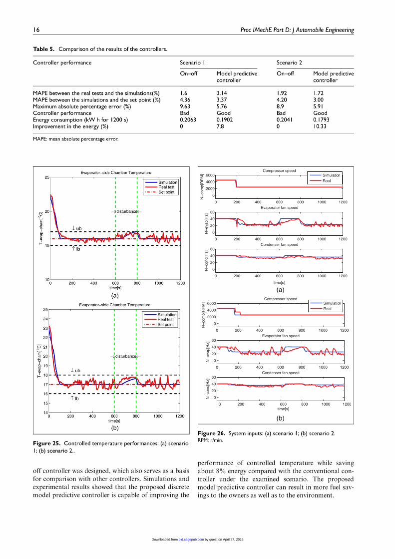
off controller was designed, which also serves as a basisfor comparison with other controllers. Simulations andexperimental results showed that the proposed discretemodel predictive controller is capable of improving the

performance of controlled temperature while savingabout 8% energy compared with the conventional con-troller under the examined scenario. The proposedmodel predictive controller can result in more fuel sav-ings to the owners as well as to the environment.

Table 5. Comparison of the results of the controllers.

Controller performance Scenario 1 Scenario 2

On–off Model predictivecontroller

On–off Model predictivecontroller

MAPE between the real tests and the simulations(%) 1.6 3.14 1.92 1.72MAPE between the simulations and the set point (%) 4.36 3.37 4.20 3.00Maximum absolute percentage error (%) 9.63 5.76 8.9 5.91Controller performance Bad Good Bad GoodEnergy consumption (kW h for 1200 s) 0.2063 0.1902 0.2041 0.1793Improvement in the energy (%) 0 7.8 0 10.33

MAPE: mean absolute percentage error.

Figure 25. Controlled temperature performances: (a) scenario1; (b) scenario 2..

Figure 26. System inputs: (a) scenario 1; (b) scenario 2.RPM: r/min.




Acknowledgements

The authors would like to acknowledge the technicalsupport of Automotive Partnership Canada and theCool-it Group.

Declaration of Conflicting Interests

The author(s) declared no potential conflicts of interestwith respect to the research, authorship, and/or publi-cation of this article.

Funding

The author(s) disclosed receipt of the following finan-cial support for the research, authorship, and/or publi-cation of this article: This work was supported by theAutomotive Partnership Canada and the Cool-itGroup.

References

1. Dincxmena E and Guvencx BA. A control strategy for par-

allel electric vehicles based on extreme seeking. Veh Sys-

tem Dynamics 2012; 50(2): 199–227.2. Lust EE. System-level analysis and comparison of long-

haul truck idle-reduction technologies. MSc Thesis, Uni-

versity of Maryland, College Park, Maryland, USA,

2008.3. Morshed MR. Unnecessary idling of vehicles: an analysis

of the current situation and what can be done to reduce it.

MSc Thesis, McMaster University, Hamilton, Ontario,

Canada, 2010.4. Khayyama H, Nahavandia S, Hub E et al. Intelligent

energy management control of vehicle air conditioning

via look-ahead system. Appl Thermal Engng 2011; 16:

3147–3160.

5. Liu JY, Zhou HL and Zhou XG. Automotive air condi-

tioning control – a survey. In: International conference on

electronic and mechanical engineering and information

technology, Harbin, Heilongjiang, People’s Republic of

China, 12–14 August, 2011, pp. 3408–3412. New York:

IEEE.6. Chiara F and Canova M. A review of energy consump-

tion, management, and recovery in automotive systems,

with considerations of future trends. Proc IMechE Part

D: J Automobile Engineering 2013; 227(6): 914–936.7. Budde-Meiwes H, Drillkens J, Lunz B and Muennix J. A

review of current automotive battery technology and

future prospects. Proc IMechE Part D: J Automobile

Engineering 2013; 227(5): 761–776.8. Johri R and Filipi Z. Optimal energy management of a

series hybrid vehicle with combined fuel economy and

low-emission objectives. Proc IMechE Part D: J Automo-

bile Engineering 2014; 228(12): 1424–1439.9. Jalaliyazdi M, Khajepour A, Chen S and Litkouhi B.

Handling delays in stability control of electric vehicles

using MPC. SAE paper 2015-01-1598, 2015.10. Kania M, Koeln J, Alleyne A et al. A dynamic modeling

toolbox for air vehicle vapor cycle systems. SAE paper

2012-01-2172, 2012.11. He XD. Dynamic modeling and multivariable control of

vapor compression cycles in air conditioning systems. PhD

thesis, Massachusetts Institute of Technology, Cam-

bridge, Massachusetts, USA, 1996.12. MacArthur JW and Grald EW. Unsteady compressible

two-phase flow model for predicting cyclic heat pump

performance and a comparison with experimental data.

Int J Refrig 1989; 12(1): 29–41.13. Rasmussen BP and Alleyne AG. Dynamic modeling and

advanced control of air conditioning and refrigeration

systems. ACRC Technical Report 244, Air Conditioning

and Refrigeration Center, University of Illinois, Urbana,

Illinois, USA, 2006.14. Wedekind GL, Bhatt BL and Beck BT. A system mean

void fraction model for predicting various transient phe-

nomena associated with two-phase evaporating and con-

densing flows. Int J Multiphase Flow 1978; 4: 97–114.15. Li B. Dynamic modeling and control of vapor compression

cycle systems with shut-down and start-up operations. MS

Thesis, University of Illinois at Urbana–Champaign,

Champaign, Illinois, USA, 2009.16. Eldredge BD and Alleyne AG. Improving the accuracy

and scope of control-oriented vapor compression cycle

system models. ACRC Technical Report 246, Air Condi-

tioning and Refrigeration Center, University of Illinois,

USA, 2006.17. Fasl JM. Modeling and control of hybrid vapor compres-

sion cycles. MS Thesis, University of Illinois at Urbana–

Champaign, Champaign, Illinois, USA, 2013.

18. Shah R, Alleyne AG, Bullard CW et al. Dynamic model-

ing and control of single and multi-evaporator subcritical

vapor compression systems. ACRC Technical Report

216, Air Conditioning and Refrigeration Center, Univer-

sity of Illinois, Urbana, Illinois, USA, 2003.19. Rasmussen BP. Control-oriented modeling of transcritical

vapor compression systems. MS Thesis, University of Illi-

nois at Urbana-Champaign, Champaign, Illinois, USA,

2002.20. Li B, Jain N, Mohs WF et al. Dynamic modeling of refri-

gerated transport systems with cooling-mode/heating-

mode switch operations. HVAC&R Res 2012; 18(5): 974–

996.21. McKinley TL and Alleyne AG. An advanced nonlinear

switched heat exchanger model for vapor compression

cycles using the moving-boundary method. Int J Refrig

2008; 31: 1253–1264.22. He XD, Liu S, Asada HH et al. Multivariable control of

vapor compression systems. HVAC&R Res 2011; 4(3):

205–230.23. Lee J, Kim J, Park J et al. Effect of the air-conditioning

system on the fuel economy in a gasoline engine vehicle.

Proc IMechE Part D: J Automobile Engineering 2013;

227(1): 66–77.24. Dhand A and Pullen K. Optimal energy management for

a flywheel-assisted battery electric vehicle. Proc IMechE

Part D: J Automobile Engineering 2015; 229(12): 1672–

1682.25. Refrigerant reference guide. 4th edition. Philadelphia,

Pennsylvania: National Refrigerants, Inc., 2006. http://

www.refrigerants.com/ReferenceGuide2006.pdf.26. Salim MM. Potential for expanders in a mobile carbon

dioxide air-conditioning system. Proc IMechE Part D: J

Automobile Engineering 2009; 224(2): 219–228.27. Nejad EK, Hajabdollahi M and Hajabdollahi H. Model-

ing and second law based optimization of plate fin and

Huang et al. 17



tube heat exchanger using MOPSO. J Appl Mech Engng

2012; 2: 1000118.28. Jabardo JM and Mamani WG. Modeling and experimen-

tal evaluation of parallel flow micro channel condensers.J Braz Soc Mech Sci Engng 2003; 25(2): 107–114.

29. Borrelli F, Bemporad A and Morari M. Predictive con-

trol. Draft. 2012. http://www.mpc.berkeley.edu/mpc-course-material (in preparation).

30. Ferreau HJ, Arnold E, Buchner A et al. qpOASES user’s

manual, version 3.0. Leuven: KU Leuven, 2014.

Appendix 1

Notation

hge enthalpy of the vapour refrigerant at theevaporator inlet

hic enthalpy of the refrigerant at thecondenser inlet

hie enthalpy of the refrigerant at theevaporator inlet

his isentropic enthalpy of the refrigerant inthe compressor

hle enthalpy of the liquid refrigerant at theevaporator inlet

hlgc latent enthalpy of the refrigerant at thecondenser inlet

hlge latent enthalpy of the refrigerant at theevaporator inlet

hoc enthalpy at the condenser outletj Colburn factorLc total length of the condenser tube wallLe total length of the evaporator tube wallm total mass of the heat exchanger_mcomp mass flow rate of the refrigerant through

the compressormpipe total mass of the refrigerant in the pipes_mv mass flow rate of the refrigerant through

the expansion valve

Ncomp compressor speedNcond control input of the condenser fanNevap control input of the evaporator fanPc pressure of the condenserPe pressure of the evaporatorPr Prandtl number for airS slip ratioSt Stanton numberTa air temperature around the heat

exchangerTic temperature of the refrigerant at the

condenser inletTrc saturation temperature of the refrigerant

in the condenserTre saturation temperature of the refrigerant

in the evaporatorTsh temperature in the superheated sectionVd volumetric displacement of the

compressor�gc mean void fraction of the two-phase

section of the condenser�ge mean void fraction of the two-phase

section of the evaporatorha adiabatic efficiency of the compressorhvol volumetric efficiency of the compressorrgc density of the vapour refrigerant in the

condenserrge density of the vapour refrigerant in the

evaporatorrlc density of the liquid refrigerant in the

condenserrle density of the liquid refrigerant in the

evaporatorrref density of the refrigerantrv density of the refrigerant through the

valve




Appendix 2

The complete non-linear and linearized models at thecurrent operating point are given in Table 6.

Table 6. The complete non-linear and linearized models.

_x f(x, u) f12x_mv

dhge

dPe+ aiAi

leLe

dTre

dPe

� �.rlehlgeAe 1� �geð Þ� �

y g(x, u) f13x � aiAilerlehlgeAe 1� �geð ÞLe

u [Ncomp, Nevap, Ncond]T f22x

_mvdhle

dPe� aiAi

leLe

dTre

dPe

� �.hlgeAeLe

drge

dPe

x [le, Pe, Twe, Pc, Twc, Tcargo]T f23x

aiAile

.hlgeAeL

2e

drge

dPe

y Tcargo f24x_mv

dhie

dPc

.hlgeAeLe

drge

dPe

f =

f1f2f3f4f5f6

26666664

37777775

_mv hge � hie

� �� aiepDiele Twfe � Tre

� �rlehlgeAe 1� �geð Þ

_mvhie � hle

hlge� _mcomp +

aiepDiele Twfe � Tre

� �hlge

�AeLe

drge

dPe

aoeAoe Tae�Twfeð Þ�aiepDiele Twfe�Treð Þ�aieshpDie(Le�le) Twfe�Treð ÞCpmð Þ

we

_mcom �aicpDiclc Trc � Twcð Þ

hlgc

.AcLc

drgc

dPc

_mcomp �aicpDiclc Trc � Twfc

� �hlgc

�Cpm� �

wc

_Qout � aoAole Ta � Tweð ÞMCð Þair

2666666666666666666664

3777777777777777777775

f32x aiAidTre

dPe

.Cpm� �

we

f33x �aiAi + aoAodTa

dTwe� 1

� ��Cpm� �

we

f36xaoAo

dTa

dTcargo

�Cpm� �

we

f41x �aicAic Trc � Twcð Þ∂lc=∂le�

hlgcAcL2c

drgc

dPc

f44x �aicAiclcdTrc

dPc

�hlgeAcL

2c

drgc

dPc

f45xaicAiclc

�hlgeAcL

2c

drgc

dPc

g(x, u) x6 f54xaicAic

dTrc

dPc

�Cpm� �

wc

Ae f11x f12x f13x f14x 0 0f21x f22x f23x f24x 0 00 f32x f33x 0 f35x 0

f41x 0 0 f44x f45x 00 0 0 f54x f55x 0

f61x 0 f63x 0 0 f66x

26666664

37777775

f55x �aicAic + aocAocdTac

dTwc� 1

� ��Cpm� �

wc

f61x �aoAo Ta � Tweð ÞMCð Þair

f63x �aoAoledTa

dTwe� 1

� ��MCð Þair

f66x �aoAoledTa

dTcargo

� ��MCð Þair

Be f11u 0 0f21u f22u 00 0 f33u

0 f42u 00 0 00 0 f63u

26666664

37777775

f11u � hie � hge

� � d _mv

duv

�rlehlgeAe 1� �geð Þ

f21u hie � hle

hlge

d _mv

duv

�AeLe

drge

dPe

f22u � d _mcomp

dNcomp

�AeLe

drge

dPe

f33u dao

dNevapAo Ta � Tweð Þ+ aoAo

dTa

dao

dao

dNevap

�Cpm� �

we

Ce 0 0 0 0 0 1½ � f42u d _mcomp

dNcomp

�AcLc

drgc

dPc

f11x aiAi Twe � Treð ÞrlehlgeAe 1� �geð ÞLe

f63u � dao

dNevapAole Ta � Tweð Þ � aoAole

dTa

dao

dao

dNevap

.MCð Þair

Huang et al. 19



Documents

Proc IMechE Part D: Modelling and optimal energy …mbahrami/pdf/2016/Modelling and optimal energy-saving... · shutdown period by considering different ... the model more complex