Embed Size (px)
Citation preview

? 8 2 - 2 9 0 - 2 2
RTI/2094/02-02Fr
NASA Contractor Report 165926
PROBLEMS RELATED TO THEINTEGRATION OF FAULT-TOLERANTAIRCRAFT ELECTRONIC SYSTEMS
Contract Number NAS1-16489
NASANational Aeronautics andSpaee Administration
'": Langley Research CenterI Hampton,Viriginia?23665'
NASA Contractor Report 1G5926
PROBLEMS RELATED TO THEINTEGRATION OF FAULT-TOLERANTAIRCRAFT ELECTRONIC SYSTEMS
J. A. Bannister, K. Trivedi,V. Adlakha, and T. A. Alspaugh, Jr.
Research Triangle InstituteResearch Triangle Park, North Carolina
Contract NAS1-16489June 1982
NASANational Aeronautics andSpace Administration
Langley Research CenterHampton, Virginia 23665

PREFACE
This report was prepared by the Research Triangle Institute, ResearchTriangle Park, North Carolina, for the National Aeronautics and Space
Administration under Task 2 of Contract No. NAS1-16489. The research was
conducted under the direction of personnel in the Flight Electronics
Division, Langley Research Center. Mr. Milton Holt was the LangleyTechnical Representative for this task.
Development of the methodology has been a team effort, with signifi-cant contributions made by Milton Holt and Rick Butler of Langley Research
Center.Joseph A. Bannister was the RTI Project Manager for the study.The authors of this report are:
J. A. BannisterK. Trivedi
V. AdlakhaT. A. Alspaugh, Jr.
Use of commercial products or names of manufacturers in this report does
not constitute official endorsement of such products or manufacturers,
either expressed or implied, by the National Aeronautics and SpaceAdministration.

TABLE OF CONTENTS
1.0 INTRODUCTION 1
2.0 DESIGN OF THE HARDWARE FOR AN INTEGRATED AIRCRAFTELECTRONIC SYSTEM . 7
2.1 A Taxonomy of Computing Systems Capableof Concurrent Instruction Execution 72.1.1 Motivations for the use of
multiprocessor systems 82.1.2 Taxonomic framework 92.1.3 Previous taxonomies of
multiprocessor systems 92.1.3.1 Flynn's taxonomy 102.1.3.2 Anderson and Jensen's
taxonomy 132.1.3.3 The taxonomy of Davis,
Denny and Sutherland 262.1.3.4 Siewiorek's taxonomy 28
2.1.4 A proposed taxonomy 302.2 A Methodology for the Design of
Multiprocessor Systems 322.2.1 Functional requirements of the system 322.2.2 Measures for the evaluation of systems 352.2.3 Tools for the methodology 39
2.2.3.1 Automatic generation ofreliability functions forPMS structures 39
2.2.3.2 Simulation to determineperformance. . 41
2.3 A Strawman Fault-Tolerant IntegratedAircraft Electronic System 41
3.0 ALGORITHMS AND CONTROL STRUCTURES FOR AN INTEGRATEDAIRCRAFT ELECTRONIC SYSTEM 45
3.1 Managing System Resources 453.1.1 Scheduling of real-time fault-tolerant
systems 453.1.1.1 General scheduling theory 453.1.1.2 Scheduling repeatedly requested
tasks subject to hard real-timedeadlines 49
3.1.2 Task allocation for the derivation oftimely schedules 523.1.2.1 Mathematical formulation of the
task allocation problem 533.1.2.2 Heuristic approach to the task
allocation problem 583.1.2.3 Evaluation of the heuristic
algorithm for task allocation 60
TABLE OF CONTENTS(Continued)
3.1.2.4 Performance guarantees for arestricted task allocationproblem 613.1.2.4.1 Difficulty of the
restricted taskallocation problem 64
3.1.2.4.2 An approximationalgorithm and itsperformance guarantee .... 66
3.1.3 Task allocation for reliabilitymaximization 80
3.2 Discussion of the Role of Software Design 813.2.1 Introduction to classical engineering
design methodology 813.2.2 The classical engineering design
methodology 823.2.2.1 Abstraction 823.2.2.2 The black box 833.2.2.3 Specifications and testing 833.2.2.4 The design process 843.2.2.5 Iterative convergence 863.2.2.6 Recursive decomposition 863.2.2.7 Documentation 863.2.2.8 Pilot operation 88
3.2.3 Software engineering 883.2.3.1 Abstraction 883.2.3.2 Black box 883.2.3.3 Specification and test 893.2.3.4 The design process 893.2.3.5 Iterative convergence 893.2.3.6 Documentation 90
3.2.4 Software engineering tools and techniques .... 913.2.4.1 A set of documents 913.2.4.2 Formal languages 913.2.4.3 Modularity and information hiding. ... 913.2.4.4 Reference vs. statement in
documentation 923.2.4.5 Simulation 92
4.0 CONCLUSIONS AND FURTHER WORK 93
4.1 Additional Tools Required 934.2 Techniques and Theoretical Work Needed 944.3 Peer Review of Specific Systems 94
v-i

TABLE OF CONTENTS(Continued)
Page
REFERENCES 95
APPENDICES 99
A 99B 103C 109
vn

LIST OF FIGURES
FigureNo. ~ Title Page
1.1 Past Aircraft Electronic System 2
1.2 Current Aircraft Electronic System 3
1.3 Future Integrated Aircraft Electronic System 5
2.1 Models of Computer Systems 11
2.2 Flynn's Partitioning of the Design Space 12
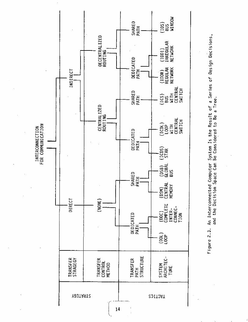
2.3 An Interconnected Computer System Is the Resultof a Series of Design Decisions, and the DecisionSpace Can Be Considered to Be a Tree 14
2.4 DDL (Loop) 16
2.5 DDC (Complete interconnection) 17
2.6 DSM (Multiprocessor) 18
2.7 DSB (Global bus) 19
2.8 ICDS (Star) 20
2.9 ICDL (Loop with central switch) 21
2.10 ICS (Bus with central switch) 22
2.11 IDDR (Regular network) 23
2.12 IDDI (Irregular network) 24
2.13 IDS (Bus Window) 25
2.14 The function of a path is to provide communicationthe path's structure is indicated by its topology.The function of an element is to perform certainoperations and the element's most importantstructural feature is its granularity 27
2.15 Important Aspects of Element Operation 29
2.16 Multiple-Processor Design-Space Parameters 31
2.17 Multiple-Processor Design-Space Parameters 33
2.18 Elements of the Proposed Design Methodology 34
IX

LIST OF FIGURES(Continued)
Page
2.19 Reliability modeling at the PMS level 42
2.20 DDC Architecture for Aircraft Electronics 44
3.1 Priority List Scheduling Algorithm 50
3.2 Example of the Construction of t and s 69
3.3 Cost Preserving Transformation of the OptimalAssignment by Step (1) 71
3.4 Assignment After Application of Step (1) andRenumbering 72
3.5 Cost Preserving Transformation of the OptimalAssignment by Step (2) 73
3.6 Final Assignment After Transformation by Steps(1) and (2). The Transformed Assignment CostsNo More Than the Optimal Assignment 74
3.7 q^(t) Cannot Have One Step 77
q*(t) Cannot Have Three or More Steps 78
3.8 Steps in the Design Process 85
3.9 Iterations for Improving Abstractions 87

LIST OF TABLES
TableNo. Title Page
1.1 Summary of System Characteristics 6
2.1 Aircraft Electronic Functions for All Flight Phases . . 36
2.2 Reliability Requirements 37
2.3 Computational Requirements 38
2.4 Reliability, Performance and Cost of GenericClasses of Multiprocessor Systems. . . 40
3.1 Processor Utilization 62
3.2 Processor Utilization and Memory 63

1.0 INTRODUCTION
In recent years, electronics in commercial transport aircraft have be-come increasingly sophisticated as the functions of flight control,
guidance, navigation, propulsion control and communication have steadilybeen enhanced through the use of programmed digital hardware. A
continuation of this trend is reflected in the desire to fully integrateaircraft electronic functions. This report is directed at the
identification of a methodology for the design of systems that fullyintegrate the aircraft electronic functions mentioned above.
System integration is measured by the ability of separate tasks toshare system resources and exchange information. Past aircraft electronicsystems had a low level of integration. A typical system as shown inFigure 1.1, had the following salient system characteristics:
• There was a proliferation of dedicated, independent processors.
f Each processor viewed itself as the center of the universe. Therewas no communication between processors.
• Tasks were rigidly segregated. For instance, flight control func-tions and navigation functions were performed by physically sepa-rate subsystems.
t Since processors did not communicate, algorithms and data struc-tures could not exploit concurrency.
• The lack of hardware redundancy made it necessary to use mechanicalbackup.
• Analog technology permeated the system.
Current aircraft electronic systems reflect an increase in integra-
tion, as typified by the aircraft electronics of the Boeing 757. A func-tional description of this system is illustrated in Figure 1.2. Character-
istics include:'
• Specialized processors are dedicated to specific tasks.
t Interprocessor communication is limited to a restricted subset ofprocessors.

PAST AIRCRAFT ELECTRONIC SYSTEM
VV COMMUNICATIONSV
_L
COCKPIT
V
oo
NAVIGATION
LANDING
SENSORS AUTOPILOT
ACTUATORS
DISPLAYS
Figure 1.1

CURRENT AIRCRAFT ELECTRONIC SYSTEM
Mode control panel
Intra-system communicalions—mostly data buses and discretes
B O E I N G 757
Figure 1.2
3 i

• Tasks are segregated. /
t Some algorithms cooperate to take advantage of concurrency. How-ever, the number of cooperating algorithms is still far belowpotential.
• The use of hardware redundancy is ad hoc rather than systematic.Mechanical backup is still necessary.
• Extensive analog technology is still present.
One can extrapolate the historical tendency of aircraft electronicstoward integrated systems. The functional elements of a postulated futuresystem are shown in Figure 1.3. Some of its characteristics are:
• Processors are general-purpose rather than specialized. This en-hances the modularity and flexibility of the system.
t There is full interprocessor communication. This permits increasedinformation utilization by processors. It also allows the systemto globally monitor itself.
• Tasks are fully integrated. Any processor can perform any task.This increases system flexibility and makes possible reconfigura-tion and graceful degradation.
• Full interprocessor communication, processor modularity and taskintegration make it possible to fully exploit the power of con-currency.
• A systematic use of hardware redundancy exists in order to achieveultrahigh reliability.
• The trend is toward fully digital processing elements.
A matrix comparing the characteristics of past, present and future
systems is shown in Table 1.1.The remainder of this report will consider the establishment of a
methodology to identify and design fault-tolerant integrated aircraft elec-tronic systems. This study proceeds by considering the design of the hard-ware for an integrated aircraft electronic system, and questions relating
to the programming and control of the system.

J F H T U R F INTEGRATED AIRCRAFT ELECTRONIC SYSTEM
I
COMMUNICATION
LINKS
PROCESSOR-MEMORY
PROCESSOR-MEMORY
PROCESSOR-MEMORY
PROCESSOR-MEMORY
PROCESSOR-MEMORY
PROCESSOR-MEMORY
PROCESSOR-MEMORY
PROCESSOR-MEMORY
PROCESSOR-MEMORY
PROCESSOR-MEMORY
Figure 1.3N;
5

00o
-I-Joo
i-O)
-(->On3S_(O£o
O)
S-tO
OO
O)
J3
0
0c:.coO)
1—
oO)i-i_3ud0
co
•1 —-4_>to1*4
•r—r—(Oo0
c0
.J3rO^_OJQ.OO
O)OC<o4.O)r^
01—4Ji —3fO
u_
£>•r-4_fO
r—~^
~UOs:
O)4_1OO
>^OO
enOr^toC
«£
~CJC
• i—r^CO
oo
N/ -£5 (/)
oo O) oon3 N O)
I— •!- 0•— O
JC <O S-O O Q.t3 ^3
UJ — 1 fO
•4-*C(Dt/)r*><
>^<^ n—rO
-o uQ^ *r—> C Q.O) "3 3
•r— f~ NXJ= O OO O) <O<: s: co
£1 0
i — O> 00n3 oo oo•i- O O)O Q. OO) i- OQ- 3 s_
00 Q- Ou
^>00ro0-
1
T3 "fO CD•i- -(-> Oi_ -r- i—o CD tO^> <r~ c~31 Q <
O
Q.0
S
0
0JS.J T3 oooo Q} oofO M O)
|— -r- 0r— O
O O Q-f& ^J
UJ — 1 to
00
00 4-»fO (O
1— i-0)
O) Q-E 00 O
oo o
•
O) +>^ 5o "O ^*>*~~
1C O 03T3 COd) "O fO •»—> 0) T3 C Q.O) 4-> C <T5 3•i- -r- 3 JC _i/:^: E "o o oO <r* O> O) ftj
«a: _ i a: s: OQ
00s-
1 0r— O! 00to oo oo•i- O O)O Q. OO) i- OQ. 3 S_
00 Q- D.
cO)00O)i-Q.
<O•4_>
•r—CD
•r—Q
r^toJ3O
r—CD
E
S- 0o M- -*:00 1_ 0000 O) fOO) Q- 1—o
>i 0 >> >>c s_ ITS c:<i Q- SI «C
0
4-> O) S-fO ^^ fO t^-S- .0 S- 0
Q, oo C ••— 00 j*O 00 O -Q -M 00o o E s- oi <e<_> a. <: =t oo i —
0)00
>^ja o >>•r- O
T3 -(-> • CQ^ 'O QJ *"O> E S T3O) O) T3 C
••--(-> a: 3_G 00 T3O >»4— O)<: oo o a:
oo
1 Oi — Q) oo<T5 00 OOS- O O>O) Q. Oc s_ oO) 3 S-
CD Q. Q.
Ol
31 '
31 1
2.0 DESIGN OF THE HARDWARE FOR AN INTEGRATED AIRCRAFT ELECTRONIC SYSTEM
In general, programmed systems such as integrated aircraft electronic
systems can be divided into two major components: hardware and software.The design of a system's software traditionally follows the design of itshardware, since the activity of programming a system depends upon the pre-existence of the system. In this chapter the design of the hardwarecomponent of the system is discussed.
The system hardware design will be discussed first in terms of a tax-onomy of systems that are appropriate for program-controlled aircraft elec-tronics. A taxonomy is a powerful tool in system design since it allowsone to systematically categorize a potentially unbounded number of possiblesystem designs. Having thus categorized the designs, one is in the posi-tion to determine which systems are suitable for the intended application.Thus, it is possible to select a specific system. After establishing the
taxonomy, a methodology for choosing a suitable hardware structure for thesystem will be considered. Having done this, the methodology will be sup-plied to select a candidate integrated avionic system.
2.1 A Taxonomy of Computing Systems Capable of ConcurrentInstruction Execution
The purpose of this section is to propose a taxonomy of computingsystems that are capable of concurrent instruction execution. Such systemsare often referred to as concurrent, parallel or multiprocessor systems.
This section effectively ignores nonconcurrent, nonparallel or uni-processor systems for several reasons. First, in the aircraft electronicssuite, a large number of functions must be simultaneously performed. This
suggests that a computing system that performs these functions must be ca-pable of simultaneous and independent instruction execution. It is unlike-ly that a nonconcurrent system could be time-shared by these functions in
any effective manner. Second, since avionics perform extremely criticalfunctions, there is a driving need to ensure the reliability of the system.Fault-tolerant methods are the proven approach to achieve high reliability.

These methods rely on hardware redundancy to tolerate faults in the system.Thus, system modules, whose function it is to interpret and execute programinstructions, are replicated. By virtue of this redundancy, such a systemis capable of independent, concurrent instruction execution. One can see,therefore, that a concurrent system is the only reasonable alternative forany candidate integrated avionic system. Thus, the taxonomy will dealexclusively with concurrent systems.
2.1.1 Motivations for the use of multiprocessor systems. - The powerof multiprocessor systems is derived from their ability to achieve algo-rithmic speedup over uniprocessor systems. A multiprocessor system isunderstood to be any programmed system of two or more processors capable ofindependent, simultaneous instruction execution and information exchangevia some interconnection mechanism (See ref. 30).
In addition to the high speed capability, there are many reasons (Seeref. 30) for employing multiprocessor systems in integrated flight elec-tronic systems. These reasons include:
Load sharing. In the event that one processor has a heavier load thanthe other processors in the system, some of its load can be redistrib-uted to the other processors.
Peak computing power. It is possible to devote the entire system to asingle task.
Performance/cost. There is an abundance of small processors with aninstructions/second/dol1ar ratio superior to that of large "superprocessors."
Graceful degradation. One can design multiprocessor systems with nocentral critical components. Failures may then be configured out ofthe system and the remaining processors may take up all or part of thefailed unit's load.
Modular growth. One can design systems in which processors, memoriesand I/O subsystems are added incrementally.
Functional specialization. One can add functionally specialized proc-essors to improve performance for a particular application.
8

2.1.2 Taxonomic framework. - The classical paradigm for taxonomies isthe Linnaean taxonomy that is used for biological classification. Twomajor principles of a taxonomic framework are illustrated by the Linnaeantaxonomy:
1) A good taxonomy is hierarchical. That is, the subject being tax-onomized can be partitioned from a very coarse level down to avery fine level. For instance, the Linnaean taxonomy dichotomizesall life into plant and animal kingdoms; animals are further di-vided into vertebrates and invertebrates, etc. This taxonomyforms an eight-level tree structure with gradations of resolutionranging from kingdoms (coarse) to species (fine).
2) A good taxonomy is based on the functional properties of the ob-jects being classified. For example, a taxonomy based solely on amachine's physical structure is unlikely to be very useful (Seeref. 8). Thus, a taxonomy of multiprocessor systems that inte-grates structural and functional system properties in its charac-terization of these systems should be considered.
A taxonomy of multiprocessor systems should embody these two important
principles.Although a taxonomy for multiprocessor systems is desired, in reality
very few multiprocessor systems have been designed. Even fewer systemshave been built and a mere handful of relatively unsophisticated multi-processor systems are commercially available. Given such a paucity ofpractical design experience in the field of multiprocessor systems, it isnecessary to consider a taxonomy for potential as well as actual systems.
Many decisions must be made when designing a multiprocessor system.The totality of these decisions will be referred to as the "multiprocessorsystem design space." Equivalently, the term "design space" will mean thecomplete collection of actual multiprocessor system designs.
2.1.3 Previous taxonomies of multiprocessor systems. - Several taxon-omies of the multiprocessor system design space exist. Four such taxon-
omies, Flynn's (See ref. 12), Anderson and Jensen's (See ref. 1), Davis,
Denny and Sutherland's (See ref. 8), and Siewiorek's (See ref. 30), arediscussed below.
2.1.3.1 Flynn's taxonomy: Flynn's taxonomy is a well-known taxonomythat is based on the multiplicity of data and instruction streams. There
are only four classes in this taxonomy, as shown in Figure 2.1. They areSISD, SIMD, MISD and MIMD, which stand for single instruction (stream),single data (stream); single instruction (stream), multiple data (stream);multiple instruction (stream), single data (stream); and multiple instruc-tion (stream), multiple data (stream), respectively. Models of each ofthese classes are shown in Figure 2.2.
Flynn's taxonomy certainly integrates both structural and functionalproperties of multiprocessor systems. His classification of these systemsis based on extremely important system features, viz., control and storagefeatures.
However, the taxonomy is not based upon a hierarchical organization.There is only one level of classification, which leaves much to be desiredwhen one is considering the design of a system. Essentially, the onlydesign parameters that can be controlled explicitly are the multiplicities
of the instruction stream or of the data stream. Clearly, much more is re-quired for a taxonomy of multiprocessor systems. A further drawback of
this taxonomy is that the resolution of its classes is far too coarse.There are only four basic classes in the design space and each class may
comprise an unmanageable number of system designs.One goal of a design methodology is the ability to choose a design
that will fit the intended system application. It is desirable that, oncethe functional and operational requirements of a system have been identi-fied, there will be a methodology that is capable of selecting suitable de-signs for the system. Flynn's taxonomy refers only to instruction and data
channels. It is doubtful that one can relate these two design parametersto the given requirements in a meaningful way. Certainly, nothing is known
in the general literature that indicates how to relate these elements.This taxonomy is, therefore, unsuitable for use in a design methodology forintegrated aircraft electronic systems.
10

Controlunit
Instruction stream Arithmeticprocessor
Data stream
a) Model of an SISO computer
Instruction stream
b) Model of an SIMD computer
Instruction stream 1
Instruction stream 2
Controlunit N
Instruction stream N
Data stream 1
Data stream 2
Data stream N
Data stream
c) Model of an MISD computer
Controlunit 1
Controlunit 2
Instruction stream 1
Instruction stream 2
Arithmeticprocessor 1
Arithmeticprocessor 2
Data stream 1
Data stream 2
Controlunit N
Instruction stream N Arithmeticprocessor N
Data stream N
d) Model of an MIMD computer
Figure 2.1. Models of Computer Systems.
11

SIMD MIMD
LDen.
SISD M I S D
INSTRUCTION STREAM
Figure.2.2. Flynn's Partitioning of the Design Space.
12

2.1.3.2 Anderson and Jensen's taxonomy: The taxonomy of Anderson andJensen is primarily directed toward the classification of multiprocessorsystem interconnection structures. This taxonomy assumes three primitivenotions—the processing element (PE), which is any unit that is able toexecute instructions, and the paths and switching elements, which make upthe interconnection structure. A path is a medium through which messagescan be transferred between other system elements, e.g., wires, radio,common-carrier links. A switching element is an entity that determines thepath that a message will take, e.g., elements for routing and dispatching.The taxonomy describes the possible configurations of the threearchitectural primitives: PE's, paths and switching elements.
This taxonomy, shown in Figure 2.3, is clearly hierarchically organ-ized. The premise of this organization is that the multiprocessor designspace is considered to be a tree. Designing a system is tantamount to mak-ing a series of design decisions. In the taxonomy of Anderson and Jensenthere are four basic design decisions to be made:
1) transfer strategy2) transfer control method3) transfer path structure4) system architecture
Decisions (1) and (2) are strategic decisions; i.e., they involvevery fundamental policy decisions. Such decisions usually have a far-reaching effect on the system's operational capabilities and may have asignificant impact on such important system features as performance, relia-bility, cost effectiveness and modularity. The first decision is whetherto use direct or indirect transmission of messages from a source to a des-tination. Indirect transmission is distinguished from direct transmissionby the presence of message-switching entities between sources and destina-tions. Units such as repeaters and temporary buffers do not constitute in-direct communication mechanisms; rather they are to be considered integralparts of the direct link. Nor do preprocessing or postprocessing deci-sions applied by source or destination elements to messages imply indirec-tion. In the event that an indirect transfer strategy has been chosen, the
13
zs°O I-H
1—• I—I— <C'00LU i—I
•z. •=>o 2:o s:o: oLU Oi—z ce1-1 Ou.
ons
o• 0)ocen•^</iO)Q
M-O
t/)OJ
•i—s_O)
OO(U(U&-
M- I—
° *-M^ <u3 COI/IOJ O
OC 4->
a
d) T3.c d)•M S- .
O)(/) X3
f—I T—
enE CO) O
•4-> O(/)>, O)
OO CQ
i_ CO) <O4J O3Q. O)E yo <oO 0.
00•oQJ C
-)-> O(_> -r-O) Wlc •>-c oO OJO QS-<D CD
4-> -CC -4->
H^
-oc c
«C 03
gure
2.3
designer must also decide whether the switching of messages is to be ef-fected by a sole entity (centralized routing of messages) or by severalentities (decentralized routing of messages).
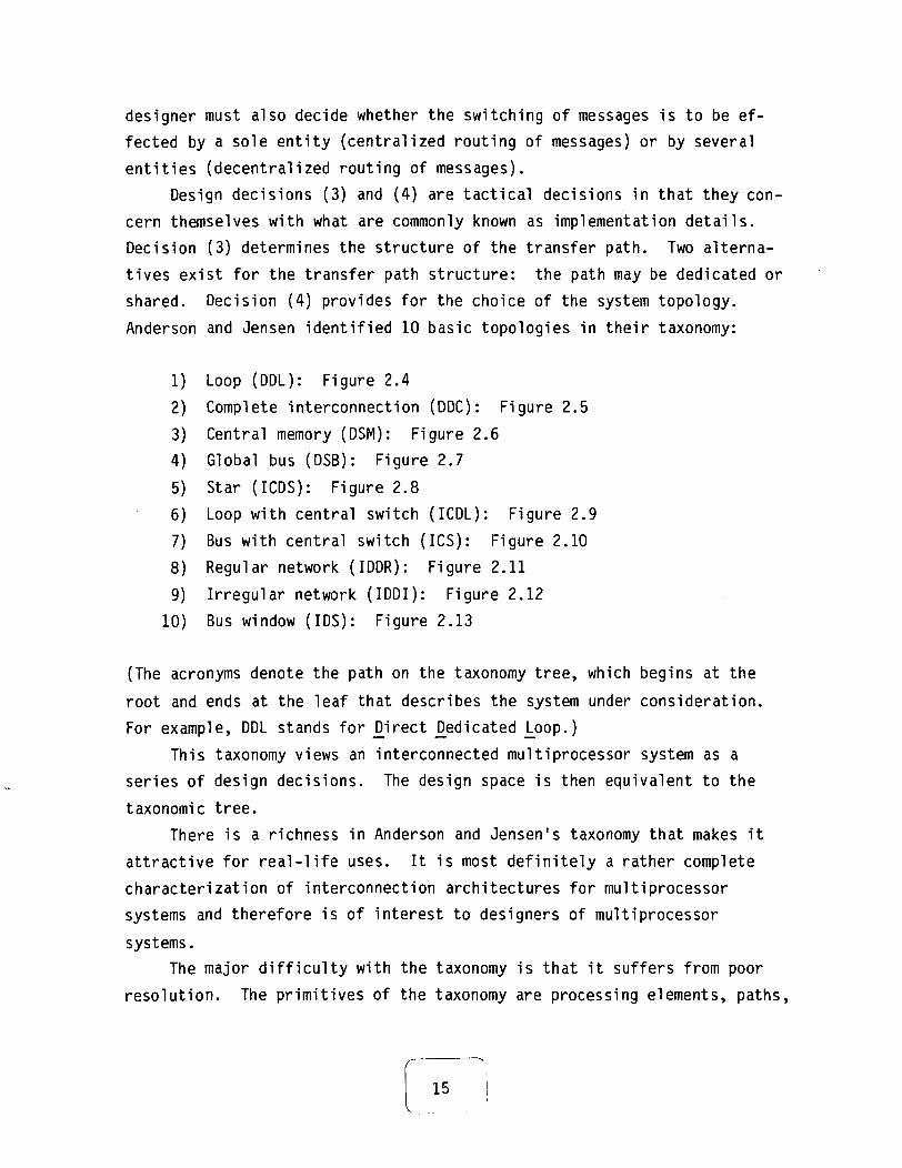
Design decisions (3) and (4) are tactical decisions in that they con-cern themselves with what are commonly known as implementation details.Decision (3) determines the structure of the transfer path. Two alterna-tives exist for the transfer path structure: the path may be dedicated orshared. Decision (4) provides for the choice of the system topology.Anderson and Jensen identified 10 basic topologies in their taxonomy:
1) Loop (DDL): Figure 2.4
2) Complete interconnection (DDC): Figure 2.5
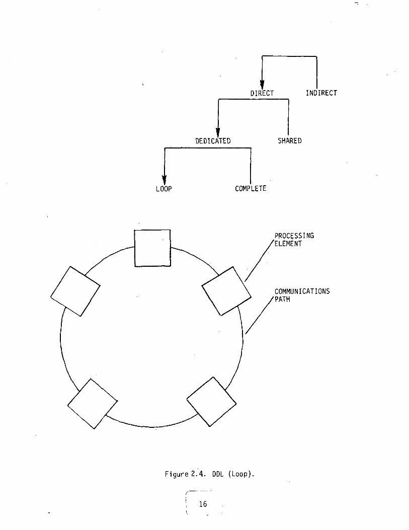
3) Central memory (DSM): Figure 2.64) Global bus (DSB): Figure 2.7
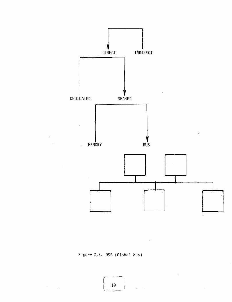
5) Star (ICDS): Figure 2.8
6) Loop with central switch (ICDL): Figure 2.9
7) Bus with central switch (ICS): Figure 2.108) Regular network (IDDR): Figure 2.11
9) Irregular network (IDDI): Figure 2.12
10) Bus window (IDS): Figure 2.13
(The acronyms denote the path on the taxonomy tree, which begins at the
root and ends at the leaf that describes the system under consideration.
For example, DDL stands for JJirect Predicated j_pop.)
This taxonomy views an interconnected multiprocessor system as aseries of design decisions. The design space is then equivalent to thetaxonomic tree.
There is a richness in Anderson and Jensen's taxonomy that makes itattractive for real-life uses. It is most definitely a rather completecharacterization of interconnection architectures for multiprocessorsystems and therefore is of interest to designers of multiprocessor
systems.The major difficulty with the taxonomy is that it suffers from poor
resolution. The primitives of the taxonomy are processing elements, paths,
15
DIRECT INDIRECT
DEDICATED SHARED
LOOP COMPLETE
PROCESSINGELEMENT
COMMUNICATIONSPATH
Figure 2.4. DDL (Loop).
16

DIRECT INDIRECT
DEDICATED SHARED
LOOP COMPLETE
Figure 2.5 DDC (Complete interconnection),
17

DIRECT INDIRECT
DEDICATED
MEMORY
SHARED
BUS
MEMORY
Figure 2.6, DSM (Multiprocessor)
18
IDIRECT INDIRECT
DEDICATED SHARED
MEMORY BUS
Figure 2.7. DSB (Global bus)
DIRECT INDIRECT
CENTRALIZED DECENTRALIZED
DEDICATED SHARED
STAR LOOP
Figure 2.8. ICDS (Star),
20

DIRECT INDIRECT
CENTRALIZED DECENTRALIZED
DEDICATED SHARED
STAR LOOP
Figure 2.9. ICDL (Loop with central switch).
21

DIRECT INDIRECT
CENTRALIZED DECENTRALIZED
DEDICATED SHARED
BUS
Figure 2.10.. ICS (Bus with central switch),
22

DIRECT INDIRECT
ICENTRALIZED DECENTRALIZED
DEDICATED SHARED
REGULAR IRREGULAR
Figure 2.1.1. I DDR (Regular network),
23

DIRECT INDIRECT
CENTRALIZED DECENTRALIZED
DEDICATED SHARED
REGULAR IRREGULAR
Figure 2.12.IDDI (Irregular network)
24

DIRECT INDIRECT
CENTRALIZED DECENTRALIZED
DEDICATED SHARED
Figure 2.13.IDS (Bus Window)
25
and switching elements. A designer would prefer a much finer resolution,
e.g., details of the memory system, bandwidth ratios, and I/O system struc-ture.
The next taxonomy attempts to reflect the multiprocessor design spaceat a higher resolution.
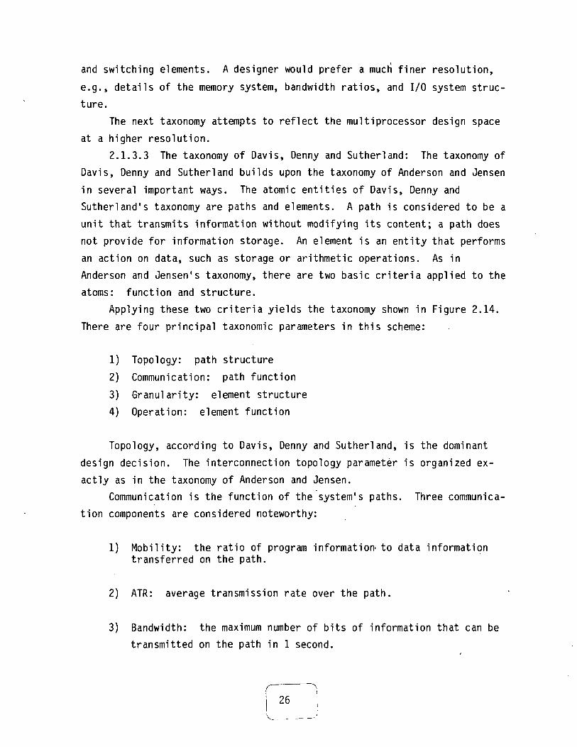
2.1.3.3 The taxonomy of Davis, Denny and Sutherland: The taxonomy ofDavis, Denny and Sutherland builds upon the taxonomy of Anderson and Jensen
in several important ways. The atomic entities of Davis, Denny andSutherland's taxonomy are paths and elements. A path is considered to be aunit that transmits information without modifying its content; a path doesnot provide for information storage. An element is an entity that performs
an action on data, such as storage or arithmetic operations. As inAnderson and Jensen's taxonomy, there are two basic criteria applied to theatoms: function and structure.
Applying these two criteria yields the taxonomy shown in Figure 2.14.There are four principal taxonomic parameters in this scheme:
1) Topology: path structure2) Communication: path function
3) Granularity: element structure4) Operation: element function
Topology, according to Davis, Denny and Sutherland, is the dominant
design decision. The interconnection topology parameter is organized ex-actly as in the taxonomy of Anderson and Jensen.
Communication is the function of the system's paths. Three communica-tion components are considered noteworthy:
1) Mobility: the ratio of program information' to data informationtransferred on the path.
2) ATR: average transmission rate over the path.
3) Bandwidth: the maximum number of bits of information that can betransmitted on the path in 1 second.
26

PATH ELEMENTS
STRUCTURE
FUNCTION
TOPOLOGY
COMMUNICATION
GRANULARITY
OPERATION
Figure 2.14. The function of a path is to provide communication andthe path's structure is indicated by its topology. Thefunction of an element is to perform certain operationsand the element's most important structural feature is itsgranularity.
27

Each of these three components may be quantified to a certain degree.Using a three-level quantification of each component, the communicationparameter can be expressed as a cross-product:
Communication =high bandwidthmedium bandwidthlow bandwidth
heavy mobilitymoderate mobilityslight mobility
high ATRmedium ATRlow ATR
The dimension or size of an element needs to be considered. For in-stance, one must be able to distinguish between a 16 x 16 array of LSI-ll'sand a 16 x 16 array of CRAY-l's. The size of the largest repeated elementis called the system's granularity. It will often suffice to discuss gran-ularity in terms of small, medium and large.
The element's operation is a functional description of the element.The dominant function of an element is the way it transforms input data tooutput data. An element is also categorized by the ratio of storage de-vices to combinational logic present in the element—this is called thememory-logic mix of the element. Other aspects of an element's operationare indicated in Figure 2.15.
2.1.3.4 Siewiorek's taxonomy: Siewiorek's taxonomy is concerned witha substantially greater number of design parameters than the previouslydiscussed taxonomies. This is appealing in that it makes it possible forthe designer of a multiprocessor system to consider a large number of tax-onomically di'stinct designs. Generally speaking, this taxonomy conveys agreat deal of information. It also treats aspects of multiprocessor systemdesign that are ignored by the other taxonomies.
Siewiorek concentrates on seven major design parameters:
1) Node types—processors, memories, switches and other devices.
2) Memory system—a decision parameter that considers the logicaladdress space and the physical organization of memory.
3) Memory switch—a decision parameter specifying the mechanism thatprovides system components access to shared memory.
4) Processor-memory data paths—a decision parameter that treatsproperties of data paths such as sharing and bandwidth.
28

co
s_CUO.O
CO)
O)
oCO
o0)0.
(O
oQ.
uri1
CM
0)S-3O)
29CD

5) I/O system—a decision parameter that deals with the logical andphysical structures of I/O.
6) Ratios--a decision parameter that determines the relationshipsthat other parameters should have to each other. Important ratiosinclude processor-memory and I/0-memory bandwidths.
7) Interprocessor communication—a decision parameter that includesdeciding how the hardware will handle interrupts and exceptions.
These decision parameters are further divided into subparameters,which allow the choice of a system to be made in an orderly and simplifiedmanner. For example, the task of selecting the appropriate memory systemis decomposed into selecting the logical and physical structures of thememory. Choosing the logical structure is further broken down into choos-ing among several memory-sharing methods (e.g., local, multiport simplex,shared-overlapped) and choosing among various alternatives for memory pro-tection (e.g., object-based, capability-based). The full taxonomy is dis-played in Figure 2.16.
2.1.4 A proposed taxonomy. - Each of the previously considered taxon-omies emphasizes certain system characteristics. Two of these—
Siewiorek's taxonomy and Anderson and Jensen's taxonomy--will greatlyinfluence a taxonomy for multiprocessor systems. Anderson and Jensen's
taxonomy does a particularly thorough job of classifying how multiprocessorsystems may be connected. Siewiorek's taxonomy has the advantage of
completeness and fineness of resolution—it is capable of examining systemsat a fine level of detail. Each of these features is desirable and will be
incorporated into the taxonomy for multiprocessor systems.The ingredient lacking in the previously discussed taxonomies is the
explicit consideration of reliability. This ingredient will be included inthe taxonomy for multiprocessor systems. Moreover, it will play a central
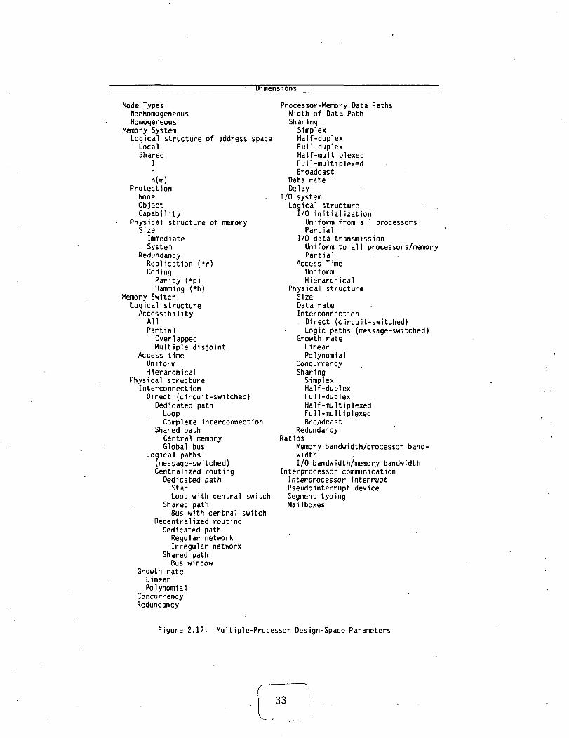
role in the design methodology, in support of which the taxonomy stands.The final taxonomy is illustrated in Figure 2.17.
30

Dimensions
Node TypesNonhomogeneousHomogeneous
Memory SystemLogical structure of address space
LocalShared
1nn(m)
ProtectionNoneObjectCapability
Physical structure of memorySize
ImmediateSystem
RedundancyReplication (*r)Coding
Parity (*p)Hamming (*h)
Memory SwitchLogical structure
AccessibilityAllPartial
OverlappedMultiple disjoint
Access timeUniformHierarchical
Physical structureInterconnectionDirect (circuit-switched)Logical paths(message-switched)
Growth rateLinearPolynomial
Concurrency
Processor-Memory Data PathsWidth of Data PathSharing
SimplexHalf-duplexFull-duplexHalf-multiplexedFull-multiplexedBroadcast
Data rateDelay
I/O systemLogical structure
I/O initializationUniform from all processorsPartial
I/O data transmissionUniform to all processors/memoryPartial
Access TimeUniformHierarchical
Physical structureSizeData rateInterconnection
Direct (circuit-switched)Logic paths (message-switched)
Growth rateLinearPolynomial
ConcurrencySharing
SimplexHalf-duplexFull-duplexHalf-multiplexedFull-multiplexedBroadcast
RatiosMemory bandwidth/processor band-widthI/O bandwidth/memory bandwidth
Interprocessor communicationInterprocessor interruptPseudointerrupt deviceSegment typingMailboxes
Figure 2.16. Multiple-Processor Design-Space Parameters
31
2.2 A Methodology for the Design of Multiprocessor Systems
The previous section was devoted to selecting a taxonomy that meets
instruction execution requirements. These requirements include the needfor a hierarchically organized taxonomy and the need for a taxonomy basedon the functional properties of the systems under study. The taxonomy formultiprocessor systems represents a merger of the taxonomies of Siewiorek
and of Anderson and Jensen.This taxonomy will serve as a framework for selecting a system design.
It views the multiprocessor design space as a tree structure with designdecisions to be made at each internal (nonleaf) node. A design methodologyshould provide designers with criteria for choosing which branch of thetaxonomy tree to take. At any given node in the tree decisions are madebased on the trade-offs in reliability, performance and cost. The inter-section of these choices is the subspace of feasible designs (see Figure2.18).
2.2.1 Functional requirements of the system. - Before one begins todesign a system, one must understand the top-level functions that the sys-tem will perform. This is a crucial activity which requires a seriouseffort. System functions may be described at several levels—from the top-
most level to a description of each software module. Typically, functionaldescriptions are in informal English prose, but it is also possible toemploy formal descriptions; in fact, formal functional specification makesit possible to apply various mathematical models in the verification or
validation of the system.A requirements specification should accompany the functional specifi-
cation. The requirements specification describes the computational (per-formance) and reliability required by each of the identified functions.
The aircraft electronics suite cleaves naturally into two components:a sensor-based (or data acquisition) system and a processor-based (or dataprocessing) system. The sensor-based system includes actuating functionsas well. The processor-based system performs the computations and arith-
metic operations necessary to aircraft electronics. The sensor-based
32
Dimensions
Node TypesNonhomogeneousHomogeneous
Memory SystemLogical structure of address space
LocalShared
1nn(m)
Protection"NoneObjectCapability
Physical structure of memorySize
ImmediateSystem
RedundancyReplication (*r)Coding
Parity (*p)Hamming (*h)
Memory SwitchLogical structure
AccessibilityAllPartial
OverlappedMultiple disjoint
Access timeUniformHierarchical
Physical structureInterconnectionDirect (circuit-switched)
Dedicated pathLoopComplete interconnection
Shared pathCentral memoryGlobal bus
Logical paths(message-switched)Centralized routingDedicated path
StarLoop with central switch
Shared pathBus with central switch
Decentralized routingDedicated path
Regular networkIrregular network
Shared pathBus window
Growth rateLinearPolynomial
ConcurrencyRedundancy
Processor-Memory Data PathsWidth of Data PathSharing
SimplexHalf-duplexFul1-duplexHalf-multiplexedFull-multiplexedBroadcast
Data rateDelay
I/O systemLogical structure
I/O initializationUniform from all processorsPartial
I/O data transmissionUniform to all processors/memoryPartial
Access TimeUniformHierarchical
Physical structureSizeData rateInterconnectionDirect (circuit-switched)Logic paths (message-switched)
Growth rateLinearPolynomial
ConcurrencySharing
SimplexHalf-duplexFull-duplexHalf-multiplexedFull-multiplexedBroadcast
RedundancyRatios
Memory bandwidth/processor band-widthI/O bandwidth/memory bandwidth
Interprocessor communicationInterprocessor interruptPseudointerrupt deviceSegment typingMailboxes
Figure 2.17. Multiple-Processor Design-Space Parameters
33

System FunctionalDescription andRequirements
Methodologyfor Design of
ReliableSystems
Methodology
for Design ofHigh-Performance
Systems
Methodology
for Design ofCost-Effective
Systems
Subspate ofFeasible Designs
Multiprocessor Design Space
Figure 2.18. Elements of the Proposed Design Methodology.
r34

system does signal processing, front-end processing and filtering, as well
as system I/O.Functions to be performed by the processor-based system are shown in
Table 2.1. The flight phases in which these functions are required arealso tabulated. Tables 2.2 and 2.3 indicate the reliability and computa-tional requirements for various functions. Computational requirements areused to estimate the processor power required to execute the functions;
reliability requirements are used to estimate the level of reliabilityappropriate to the processor-based system. As shown in the tables, air-craft electronic functions have high reliability and computational require-ments.
2.2.2 Measures for the evaluation of systems. - In this section a setof measures for evaluating multiprocessor systems are proposed and thenused in the design methodology. The significance of measures to the
methodology is that they allow system designs to be measured with respectto some desirable characteristic. One can then select those designs whosemeasures meet the postulated system requirements.
The proposed measures fall into three broad classes: reliability,performance, and cost.
Reliability measures• failure-effect: the susceptibility of a system to a single
failure• fai1ure-reconfiguration: the ability of a system to operate in
a degraded mode once a failure has occurredPerformance measures
t bottleneck: the tendency of a system's throughput to be limitedby lowered performance in a subsystem
• communication complexity: the totality of decisions made duringcommunications by source processes, destination processes orswitching entities

l/lQJ
.ea,
cC
O
co
co1-4->ua>
i,u
CJ
(U
O i.
OO I Q. Q_ O. C D C Q C Q D - I C O Q _ Q . t / ) t / > O O O O Q _ Q .
Q. Q_ Q_ o_ CO
o_ o_ co Q_ a_
10 10
O- O- f) I Q_ O_ O. -Q_ CO
Cs- oo —
4-> 4Jro ITS(j cn
01 o>I— 4JQ. "-
T3 OC •—
OS
(O UJ
l— CL 4J 4->•O O O ••- «-(O 4J 4-> 4-> (1J
<u•o
0)a)o.
a>o<o
TJ
» g
COg
s-'5
T3CO
<DE
5 o£ 4-> 4-> i-
•r- !_ 4->-M C O CC O CX O<u s: o. <-J3 E ^> <N
.Q . 4 - * ' —
( O ( O | —
O-OI-
36

tf>s_o
co
EOJ
oo.
cr0)
Of.
4-1 0)10 4-1a o
s-
•o oQJ -I—
OJ OJ O) OJ
PO CO CO CO IT)I I I I IOJ OJ OJ OJ ^ OJ OJ CO
c;o^juc
o1-cooOJ
5
«t
^o
co
l_O)
3
u.
6i-co
IOo
— 1
oIOu-O'c
4-1
-a o <uc •— "o
i— CL 4-10 0 - . -
3 3 4J
Co4-1IOcn
10s:
IO
S-<u
1— 1
UJ
0
Ol
"a.4-1
E
60
LU
Iano
<u
r—
<v<e
0
sLUs:o
_
co4JIOcn>10
IO4-1ieo
<t
«;4J
"-
CIOE
"ioXX
co4-1
14-*t/>UJ
o>T33
4->
4-*
(O eC4->
Q -0OJ
-M 0)^ Q.O) V)
U. «I
>.(tJ
Q. >>(/) <O
o 'o.u •»-.cQ- 4-»
CD 1—
O)uc
^^o
^£
cot/1
oCJ
^_J
<r•,
c
OO
(O
IOo
toCD
O
•oc3O
V-
^C'
«t
c
o
rtJ GO4-> 0nj >— *0 <
uo
-4->
c
c
£cnc
o•r-CO
§4-1t/)
t/1
O4J t-i- 4JO CCL Of> (j
CO <Uc
ll- 01_l UJ
104-1J= 4-1cn 10
cn
O •—
O) oM-IO >>t/1 4-1
<vO <4-4^ IO
IO OO 4-1
— 10S- Uu ••-
4-1
i— CQ) y
O *— */>•r— 10 QJ1/1 C Ut/i o> c:
•r- l"1 QJE 3
i— crc 10 a;•i- C I/I
o cOJ •<- OCn uIO I- OJZ 0) —O 0. E
o o4-1 CC i— OIO IO u<J "- O>
H ^ QJ•r- IO »—C 4J JD
•i- J3 S-
(/I
co
c co o <*-•i- i- O4-1 4-1U O (/»C C CO3 3 O
ui i/i in in t/itn t/i i/i V) t/i
<_> O t_>
37

(/I
Req
uire
men
t
1Cco
4->ro4^3Q.EOO
00
CM
CU
«->ro
1—
t/lC0
o
ct—4
•(—
oi-OJQ.
t/l•oS-
3^
>
O
Q.
C0
ro
Ol
S-CUQ.
<OCU
E
•u<Uto
OJ
mQ£
in oj o m o o or»- &i IO OJ LT> »-H inO O CM ro ojCM ^H r— ( f\J
CM ^o i— i in o r . mO O 0 O O O O
O 0 O 0 0 O 0
O VO CO ^" O f^- Oin r**. in - o *o <JDf— i oj oo oj in roi— 1 CM t— 1
IDOJ CO
S ^- ^- ^£) O CO O0 CO ^-CM
O O O O in O inoj m *± »o co oj
CM CM •— 1
g L o t n m o o o o o o o j o o o oo r o t — i i r > r o m « d - O ' - H * o o o o o
o o m « — ( P o m ^ - C M r o c M ^ t n r o o ^ o o
8 O O O O J O O O * - t C M O O O ' - H O Oo o o o o o o o c o o o o o o
o o o o o o o o o o o o o o o
O O O O O C M O O < — I O O O O O O
S o o o o v o o o r o o i n o o o oO O C M O ^ t f > O C J % C S J C M l D C O O J O
in IT) ^ - i— l rH OJ CM
Lfl LO O
O O O O O C M L O O ' — ' ^ " O O O O OO O O O O I O C M O i n m o o oC M O J C M O C M t — I t — 1 O J O J C M O O
in CM oj
CM in to
10 m in o ID I D C O O O O ^ ^ S - ^ O Oi— i f-H r-» m
VO OJ
ooin
•-H.— I
O
VD0UDro
8
roro
oi-
co
CUT33
4-1
«
(—
0
'CO
CU
3
U.
o
co(J•oroO
S-oroO
•DC
T3 O CUc r— -a
r— <-> 4^
o o ••-3 3 4->
CO
roOl
ro
,
1 *
OJ
»— t
sCU
"o.
3
08
LU
/•*•!
o:O
CU
^_
CU
ro00
S-o«t
o
-o1 *ro01
ro
ro
roO
=c
T?014->
Ll-
CroE
ro
O
ro
LU
CUT33
4_)
ro <f
ro »
CU4-> CUs. a.Ol en
LU «r
>^ro
O.to
O
U
.co.roS-(D
ra
Q.
Q
XCU
r—
UCro•oO
eC
cO1/1
oo
00CO
o*""*
c3OS-cs
0 S-
< 5•s *
§ 1o
o oro ro on4-> 4-1 Oro ro •— tO D <
i-O4-»• r—
Co
4-*CCU
S-
cnc
o.ciECU
oo
^_oa.o.300
CU14-_J
o1 *co
CUc
O)cLU
38
Cost measures
a cost-modularity: the incremental cost of adding an elementt place-modularity: the degree to which the location or function
of an added element is restricted• connection-flexibility: the ability to employ alternative top-
ologies, given a specific interconnection structure.
These measures are not intended to be quantitative and often takequalitative values (high, moderate, low) when applied to systems.
Table 2.4 shows how different generic families of the taxonomy varywith respect to the identified reliability, performance and cost measures.
2.2.3 Tools for the methodology. - The qualitative measures discussedabove are useful in selecting feasible designs. Once the feasible designsubspace has been isolated, however, more precision is desired in evaluat-ing the best design for this particular application. Simulation and ana-lytical tools are the time-proven means for the precise evaluation of agiven design. Some of these tools are discussed below.
2.2.3.1 Automatic generation of reliability functions for PMS struc-tures: Each of the various multiprocessor systems treated by the taxonomycan be expressed in PMS descriptions. PMS is a well-known hardware de-scription language (See ref. 3), the description of which is beyond thescope of this report. Once a set of feasible systems have been targeted,they may be translated into PMS descriptions.
The motive for describing the systems in PMS notation is the Advancedinteractive ymbolic ^valuation of Reliability (ADVISER) program (See ref.18). ADVISER is the result of a study to demonstrate the feasibility ofbuilding design tools that perform a significant portion of the reliabilityanalysis of systems. ADVISER attempts to relieve the designer of the bur-den of the traditionally complex, tedious and error-prone reliabilityanalysis of systems. The user of ADVISER essentially provides ADVISER witha PMS description of the system under examination and the failure rate de-scription of various PMS components. ADVISER ultimately produces symbolicreliability functions of the system. The scope of systems analyzable byADVISER is shown in Figure 2.19.
39

s-o
oi.a.
o>o
o<t-s_o>
IO
"oi
CO
01
l/>
t-
IO
£4J
o0
Mea
sure
sP
erfo
rman
ceas
ures
I
Re
liab
|\
Mea
sure
con
ne
ctio
nfl
ex
ibil
ity
X4-*
1 1-01 IOo •—<0 3
1 L_4J 10
O 3u-o
com
mun
icat
ion
com
ple
xity
bo
ttle
ne
cku
rati
on
cn
i*-
-re
co
10
u014-
<u1t-3
10
/
.c<J
s
LUCL.
JZu4-*
's
.cIOQ.
LUQ_
Ol.C S-U 34-» i —
'x'<oCO «*-
<Di-
.c •—10 10
CL. <t-
0)
3
UJ -i-Q_ IO
QJJC i.U 34J i—
a '«
(UL.3
JZ *—4-» •*-<O IOCL, t-
S-'3
LU i —
«
/oo
1
1
I- O<u o> cn
'
S- O<U o> cr
1- 0<u o> cn
3
loo
p b
an
dw
idth
,PE
1
ooCL
i.0oCL
•
i.O0CL
OOCt
§
'
'
•o0ocn
i
i.ooCL
i-O
R
•£O
none
ob
vio
us
'
0o
•oo0cn
1
•o0o
T30Ocn
OO
1
1
s- o01 O> cn
'
i. O01 O> cn
o>)4-> S-t- o> o o
0cn
o
mem
ory
band
wid
th
i
oo0.
-oo0cn
i
i.oo0.
T3OOcn
o
'
'
•ooocn
i
i-og.
•o0
I Ocn
low
to
mod
erat
ebu
s b
an
dw
idth
i
0oCL
i- 001 O> cn
'
i.0oQ.
i~ 0OJ O> cn
CO
o
i.0oCL
0
•ooocn
'
S-ooCL
oocn
mod
erat
e
JCu
X
ooQ.
IO
O4-> i.
O•a oO CL0cn
i.o0CL
i.ra
0
•o oo o0 0cn
QO
S-
IO<*-
•ooocn
oocn
i
•o0ocn
T3OOcn
mod
erat
elo
op
ba
nd
wid
th,
PE
, sw
itch
ing
0oCL
O0CL
0OCL
O0CL
S-o0CL
0OCL
g
t-oi.
•oo
•o0ocn
i
•oo0cn
•o0ocn
mod
erat
ebu
s b
an
dw
idth
,sw
itch
ing
O
§.
0oCL
•oO0cn
OOCL
ooCL
IO
I/Io
S-0oo.
i-og.
i.ooCL
i.0oCL
0oCL
OOCL
mod
erat
eno
ne o
bvi
ou
s
og.
0oCL
s.ooCL
4-> 11-
-o <uo -a <uO O 4->cn E 10
o4-> 1
-O 01o -a <uo o *->cn E *
o4-> 1
s--0 <Uo -o <uO O 4->cn E ia
ex.O
•aoocn
•a \0ocn
•ooocn
T3o0cn
-a0
• ocn
•oo0cn
cn
none
ob
vio
us
•o i-o o ••-O 4-» IOcn <*-
00--o 4-> 10cn t-
•o0ocn
?oi0 4-> 10cn 14-
T3 i.O O "-O 4-> IOcn V
•oOOcn
oo
•o0oCn
•oos,
T3O0cn
•aoocn
•ooocn "
•ooocn
mod
erat
ebu
s b
an
dw
idth
,sw
itch
ing
i.
IO
•oo0
us
i-IO
o0cn
LOo
40

A program such as ADVISER can then be used to further attenuate the
feasible design subspace. The output of ADVISER is simply used to concen-trate on those systems with estimated reliability ranges within the window
of postulated reliability requirements.2.2.3.2 Simulation to determine performance: A candidate system
should certainly be subject to scrutiny before plans to implement thesystem are pursued. In the absence of any physical system, simulationbecomes a necessity. Simulation is also a very cost-effective means forpredicting system behavior and fine-tuning design parameters. Simulationtechniques to deal with three performance issues—throughput, deadlock andbottleneck—will be considered below.
The Extendable Computer System Simulator II (ECSS II), a program basedon SIMSCRIPT (See ref. 19), is used principally for simulating computersystem behavior. It has the capability to model various system componentssuch as processors, memories, I/O and other devices, and queues as well asvarious attributes of these entities. It can also model certain eventsrelated to the entities' functions, e.g., arrival, processing and storage.
This tool is publicly available from the Models Directorate of FEDSIM andhas the promise of great usefulness in the proposed taxonomy.
Ramamoorthy (See ref. 26) has an approach for predicting maximumperformance of a system and for detecting the potential for deadlock in
systems. Both approaches are based, on concepts from the theory of Petrinets. In modeling systems with Petri nets the problem is that there is noeasy way to interpret the system as a Petri net; i.e., this is an art andnot a science. If this impediment can be removed, Ramamoorthy's techniqueswill indeed be attractive.
Han's (See ref. 16) approach to identifying system bottlenecks is also
based on Petri nets. The same considerations that apply to Ramamoorthy'swork also apply here. If the details of Petri net modeling can be worked
out, then bottleneck identification will be feasible.
2.3 A Strawman Fault-Tolerant Integrated Aircraft Electronic System
For the purposes of illustration and discussion a strawman system ispresented below. Examining Table 2.4 gives a rough estimate of the total
41

PMS Reliability Computation
Repairable
SystemsNonrepayable
Systems
RepairStrategies(no maintenance)
Periodic Maintenance
and Repair Strategies
Failure to
Exhaustion
Figure 2.19. Reliability modeling at the PMS level
42

figure of merit for each of the 10 different interconnection architectures.
If reliability, performance and cost are weighted as three, two and one,respectively, then a ranking of the different interconnections may be ob-tained. In calculating the figure of merit, "good" is interpreted asthree, "fair" is interpreted as two and "poor" is interpreted as one. Therelative ranking is as follows.
1) DDC
2) DSM3) IDDI
4) DSB
5) ICS
6) IDS
7) ICDS
8) DDL
9) IDDR
10) ICDL
The use of the DDC architecture, the highest ranking, will be consid-ered in a fault-tolerant integrated aircraft electronic system. The systemdesign will be divided into the design of the sensor-actuator subsystem andthe processor system. A complete interconnection structure can be immedi-ately eliminated from the sensor-actuator subsystem, since information ex-change between sensors and actuators will be limited to a few subsets ofthe entire subsystem. However, complete interconnection of sensor-actuators with processing elements will be included. Furthermore, allprocessors will be completely interconnected and fully replicated for thepurposes of fault-tolerance and reconfiguration. Processors will also havecomplete interfacing with the sensors and actuators. The strawman systemis depicted in Figure 2.20. '
43

Sensor-Actuator Subsystem
Interface betweensubsystems - fullinterconnection
between elements ofboth subsystems
Processor Subsystem
Figure 2.20. DDC Architecture for Aircraft Electronics.
44

3.0 ALGORITHMS AND CONTROL STRUCTURES FOR AN INTEGRATED AIRCRAFT
ELECTRONIC SYSTEM
In the previous chapter, the design of the hardware for an integratedaircraft electronic system was discussed. In this chapter, the softwareaspects of system design will be considered, first in terms of themanagement of system resources and then in terms of the role of softwaredesign in the overall system design.
3.1 Managing System Resources
3.1.1 Scheduling of real-time fault-tolerant systems. - In this sec-tion the general background material that is necessary for understandinghow systems are scheduled and how scheduling methods are evaluated is pro-vided, followed by the specific problem of scheduling tasks in aircraftelectronic systems.
3.1.1.1 General scheduling theory: Scheduling is a crucial aspect ofthe problem of efficiently managing the resources of a computing system.If a system has available a finite amount of certain resources (e.g. proc-essors, devices, memory) to be used by a group of competing consumers (gen-erally speaking, tasks or jobs), then it is imperative to schedule theseconsumers. The act of scheduling the consumers is essentially a directivewhich notifies the system when and for how long a consumer shall usespecific resources.
Scheduling is necessary from the point of view of making the systemwork: the tasks to be performed must be scheduled and dispatched (started)in some specific order and at certain points in time if the system is toeven begin performing its function. Hence, a mechanism for producing andinitiating schedules is inherently present in all operational systems.
The real payoff, however, stems from the fact that different schedulesmay have different overall system implications. One major system implica-tion is the cost of executing a set of tasks. In general, two differentschedules will have two different costs. Clearly, one wishes to choose theschedule with the smaller cost. Another important system implication in-volves the relative importance or criticality of the tasks. One would
45

like to be confident that the most critical tasks will always have enough
resources available to fully perform their functions. This could entailpreempting tasks of lesser criticality, but the system may nevertheless
function acceptably even when the least critical tasks are offered lessthan their requested complement of resources. A schedule controls thetasks' access to resources; therefore, scheduling plays a key role in theeffort to ensure that critical tasks are provided the resources they re-
quire (possibly at the expense of less critical tasks).The choice of the "right" scheduling strategy will thus yield a system
with desirable characteristics: reduced running costs, assurance thatcritical tasks will be performed, and efficient use of resources.
In a computing system dedicated to guidance and flight controls, taskswill have to be repeatedly executed in a real-time manner. More specifi-cally, the existence of some number of processing elements can be assumed.The number of processors may decrease as the result of hardware failures.The tasks will be ordered according to their relative importance to thegiven flight phase. These are the essential elements of the system that isto be scheduled.
Generally in scheduling multiprocessor systems, one begins with a set
of m (identical) processors
P - f P l . P2> ••" praf'
A task system for a set of processors P is a triple (T, <, M) where:
1) T = {Tj T2, .-..--,• T^J is a set'of tasks' to be executed.
2) < is an irreflexive partial ordering on T indicating the prece-dence constraints of the tasks; Ti < Tj means that T^ must
be completely executed before T..- can be started.J
3) M: T >-|x: x is a positive'real number} is a function speci-fying the execution time required by each task.
Note that a task has the same execution time for each processor.If one would like to schedule the tasks on various processors, given
such a task system, a list is created that tells, for each task, the time
46

at which it is to be started and the processor on which it is to run. Thisschedule must be consistent: two tasks cannot be scheduled to run on thesame processor at any given time. These notions are formalized by defininga schedule for a task system (T, <, M) on processor set P to be a function
S: jx: where x is a non-negative real number}—»- 2'
(2T is the set of all subsets of T). The function S must satisfy thefollowing properties:
1) |s(t) £ m for all t _> 0. No more than m processors are runningat any time.
2) There is a minimal real number w(S) such that for all t _>.S(t) = 0. w(S) is the total execution time for S.
3) U S(t) = T. All tasks get scheduled.0 <_ t <_ «(S)
4) Let t<.(T.) -- inf "t
be the starting time of task Tj.T.J « S(t) if and only if
W 1* IW +M(Ji)-
A task runs for only one uninterrupted time segment.5) If T. < T., then tc(t.) +M(T.) < tc(T,). A task may not be
I J - S I I — S J
started until its predecessors are completed.
Scheduling a task system on multiprocessors to minimize the schedule'stotal execution time (w(S), or simply w if no possibility of confusionexists) is thought to be an inherently difficult problem (i.e., the problemof determining an optimal schedule is NP-hard). This is highly unfortu-nate, as schedulers are generally required to make decisions in real-time.One is therefore forced to consider scheduling algorithms that do not giveoptimal schedules. These nonoptimal algorithms are sometimes referred toas "heuristic" algorithms. Heuristics are, strictly speaking, not algo-rithms but rather loosely applied approaches to the solution of a problem
47

(i.e., a "rule of thumb"); nonetheless, the oxymoronic phrase "heuristicalgorithm" will often be employed to refer to an algorithm that does not inall cases produce an optimal solution.
If one accepts the thesis that the general multiprocessor schedulingproblem is intractable, then one must resolve to live with lowered expecta-tions. There are basically two ways to deal with intractability. Theseare:
1) Design efficient algorithms that produce suboptimal solutions.2) Restrict the given problem so that one can design efficient algo-
rithms that still produce optimal solutions.Alternative (1) is essentially an attempt to discover algorithms whose exe-cutions require reasonable amounts of time and space and whose outputs aresuboptimal, yet acceptable. Alternative (2) attempts to discover nontrivi-al, useful subproblems of the original problem for which algorithms withreasonable time and space requirements can be designed. Furthermore, therestricted algorithm should produce optimal results.
It is necessary to digress momentarily in order to clarify what con-stitutes a reasonable algorithm or an acceptable solution. In the jargonof computer science a reasonable algorithm is one that requires space andtime that grow no faster than a polynomial function of the problem size.Even this is unrealistic since polynomials may grow very rapidly (e.g.,
10 * x ) . In practice it is common to expect a reasonable algorithm torun in quintic time and space. The other subtlety involves deciding whenan algorithm produces a "good" suboptimal solution. Usually, given analgorithm that is suboptimal, the question is posed: "Is there a guaranteethat this algorithm will never give a result that is 'x1 percent worse thanoptimal?" Given a heuristic algorithm HA for a problem P one can speak ofthe absolute performance ratio for an instance I of the problem. This isdefined to be HA(I)/OPTP(I), where OPTp(I) is the optimum for instanceI of problem P. In general, one hopes to find a constant upper (lower)bound on the absolute performance ratio for minimization (maximization)problems. It is desirable in practice to establish an upper bound of nomore than 2 or 3 (100 - 200% more than the optimum). A less desirable, butmore common, situation is when the upper bound is a function of the problemparameters rather than a constant.
48

In the face of intractability the two alternatives discussed above
have actually been employed by computer scientists.As an example of alternative (2), one could use a very simple algo-
rithm to schedule a task system on a set of processors. One such simplealgorithm is the priority list scheduling algorithm given in Figure 3.1. Aclassical result of Graham (See ref. 14) is the following.
Theorem 3.1: Let wg be the smallest possible total execution timefor a task system (T, <, M ) on a set of m identical processors P andcop|_ be the total execution time for (T, <, M) on P when scheduled by apriority list discipline. Then
Furthermore, this bound is tight; i.e., an infinite number of task systems
(Ti, <, ) exist such that
"PL
where upL is the total execution time of (T^, <, M) scheduled on P by
a priority list discipline.The above theorem is a guarantee that the priority list scheduling al-
gorithm of Figure 3.1 will always produce a schedule that is completed inless than twice the optimal completion time. Note also that the algorithmis a polynomial time algorithm (running in time proportional to mn). Thisis a premier example of a fast algorithm that gives reasonably good (but
suboptimal) schedules.3.1.1.2 Scheduling repeatedly requested tasks subject to hard real-
time deadlines: The scheduling problems discussed in the previous sectionseek to schedule tasks that are executed only once and are not subject toany deadlines. In a real-time environment, especially in control systemssuch as flight controls and guidance, the tasks will typically be repeated-ly requested and executed. Each task will have to be completed before itsnext request—this constitutes the task's inherent deadline.
The implicit assumptions in this application are:
49

Input
A set of n independent tasks with execution times mu[l..n] to be scheduled
on m processors.
Output
A schedule specified as
assign[l..n] - task i is assigned to processor assign[i]
start[l..n] - the task's start timefinish[l..n] - the task's finish time
Algorithm
0;1 to m do free[j] -* 0 od;1 to n
1;for j -« 1 to m
do if free[min] > free[j] then min-*—j fi od;assign[i] -^ min;
start[i] -* free[min];
free[min] ~* finish[i];
if omega < finish[i] then omega-* finish[i] fi
odend.
Figure 3.1. Priority List Scheduling Algorithm
50
1) The requests for each task consist of an infinite number of equal-ly spaced requests.
2) Each task must be completed before its next request.
3) The tasks are independent of each other.
4) Each task has a constant run-time.
5) The execution of a task can be divided into discrete chunks, i.e.,tasks can be scheduled preemptively.
First, in terms of how to schedule such a set of tasks on a single
processor, the fundamental question is: "How does one know when a set oftasks can be scheduled on a processor?" This question was answered by Liuand Layland (See ref. 22). If the utilization of a task is defined as itsrun-time divided by its request interval, then a set of tasks may be sched-
uled on a processor, provided that the sum of all task utilizations doesnot exceed certain scheduling constants. The scheduling constants are re-lated to the particular scheduling algorithms used. Liu and Layland stud-ied two algorithms. In the rate monotonic priority algorithm the highest
priorities are assigned to tasks with the highest utilizations; tasks arethen preemptively scheduled by using a standard priority algorithm. In the
deadline-driven algorithm, each task's priority at any given time is de-termined by the proximity of its deadline; tasks are continuously being
reprioritized and rescheduled (preemptively). Thus, according to Liu andLayland, a set of tasks may be preemptively scheduled on a processor byeither of the above algorithms as long as certain constraints are satisfiedby the set of tasks. The constraint is that the sum of the tasks' utiliza-tions shall not exceed certain scheduling constraints. For the rate mono-tonic priority algorithm and the deadline-driven algorithm, the scheduling
constants in this application are In 2 (approximately .69) and 1, respec-tively.
Dhall and Liu (See ref. 10) studied a generalization of the problemabove where multiprocessors are available. Their solution reduces the mul-tiprocessor problem to first allocating subsets of tasks to the processorsand then individually applying either the rate-monotonic priority algorithmor the deadline-driven algorithm individually to each processor and thetasks allocated to it. The problem of scheduling real-time fault-tolerant
51

systems then becomes one of allocating a set of replicated tasks to a col-
lection of processors.
3.1.2 Task allocation for the derivation of timely schedules. - Sev-eral classes of problems play key roles in the integration of fault-tolerant guidance and flight control systems. In the past, these problemswere not addressed in any systematic manner; system designers relied on in-tuition and ad hoc methods in solving these problems, or the problems were
completely ignored.Some specific classes of integration problems that warrant systematic
approaches are:- efficient resource allocation in fault-tolerant multiprocessor sy-
stems- reliable restructuring of control laws in the face of altered
flight requirements- use of parallelism in conventional control theory- methods for simplifying the programming and use of fault-tolerant
multiprocessor systems
- techniques for improving software reliability in fault-tolerantmultiprocessor systems
One very important topic in guidance and flight control systems is re-lated to two of these classes. This topic—the sizing, allocating, andscheduling of a system of processor-memories and tasks—involves the prob-lem classes, efficient resource allocation and simplification of program-ming.
Sizing, resource allocation and scheduling may be approached in twoways: statically or dynamically. The static discipline normally requiresoff-line precompilation of the allocation and schedule, relying heavily ontabular methods, thus requiring some form of involvement on the part of theprogrammer for table creation. The dynamic discipline frees the programmerfrom this onus and requires less memory.
An interesting problem addressed in the design of SIFT (See ref. 33)
is the allocation problem, which requires that tasks and processor-memoriesbe mutually allocated in such a way that processor-memory load is balanced.A special-purpose technique has been employed (See ref. 33) and the results
52

appear to be satisfactory. The results were obtained for SIFT with asmall, hypothesized task set for which strong assumptions about the proces-
sor and task characteristics were made. There is no indication that theallocation derived for SIFT could not be improved. The design of largefault-tolerant multiprocessor systems with static allocation will requirethat this problem be solved in a generic way. The initial objective is to
provide a general-purpose solution to the problem which will optimize theallocation with respect to selected target functions.
3.1.2.1 Mathematical formulation of the task allocation problem: Inconsidering a problem in which a set of tasks and a collection of process-
ors are given, the most general case is one in which all processors may bedifferent, although a uniform processor set is most likely to be encounter-ed in fault-tolerant systems. The characteristics of each processor, viz.,speed (in instructions per second) and memory capacity (in words or bytes)
are assumed to be known.Information is also available about the tasks, which are assumed to be
periodically executed. The information available on the tasks includesiteration rates (the number of times the task is requested per second), thenumber of instructions executed per iteration, and the amount of memory re-quired by the tasks (i.e., the space occupied by the program plus the maxi-mum size achieved by its activation records). Other information includes
the active and passive replication factors of the tasks: an actively rep-licated task is executed on each processor to which it is allocated, where-as a passively replicated task is not executed under'normal conditions.The passively replicated task resides in the memory of a processor and isexecuted only in the event that one of its active instances is unable to beexecuted. In that case, the passive task becomes active and the task sys-tem is reconfigured by allowing the formerly passive task to execute on itsassigned processor. Clearly, passive allocation is employed for the most
critical tasks.It is well known (See ref. 22) that periodic tasks may be well sched-
uled on a processor as long as the tasks' collective utilization of theprocessor is maintained below a certain threshold. For example, a set ofperiodic tasks may be scheduled on a processor using the rate-monotonic
53
priority algorithm or the deadline-driven algorithm, if the utilization ofthe processor is In 2 or 1, respectively.
The problem is essentially to assign the tasks to processors so thatno single processor is utilized much more than any other. For example, ifa two-processor system is considered and a set of five tasks are assigned,the tasks are T^, T2, T^, T^, Tg and the processors are P^ and P2. The
tasks have respective utilization factors of .5, .4, .3, .2, .2. If eachtask is to be actively replicated only once and no task is to be passively
replicated, there are 32 different assignments possible. Assigning Ti, T^to P and T2, T^, Tg to P2 achieves the optimum since both processors obtain
a utilization of .8, indicating that perfect balance in utilization hasbeen achieved.
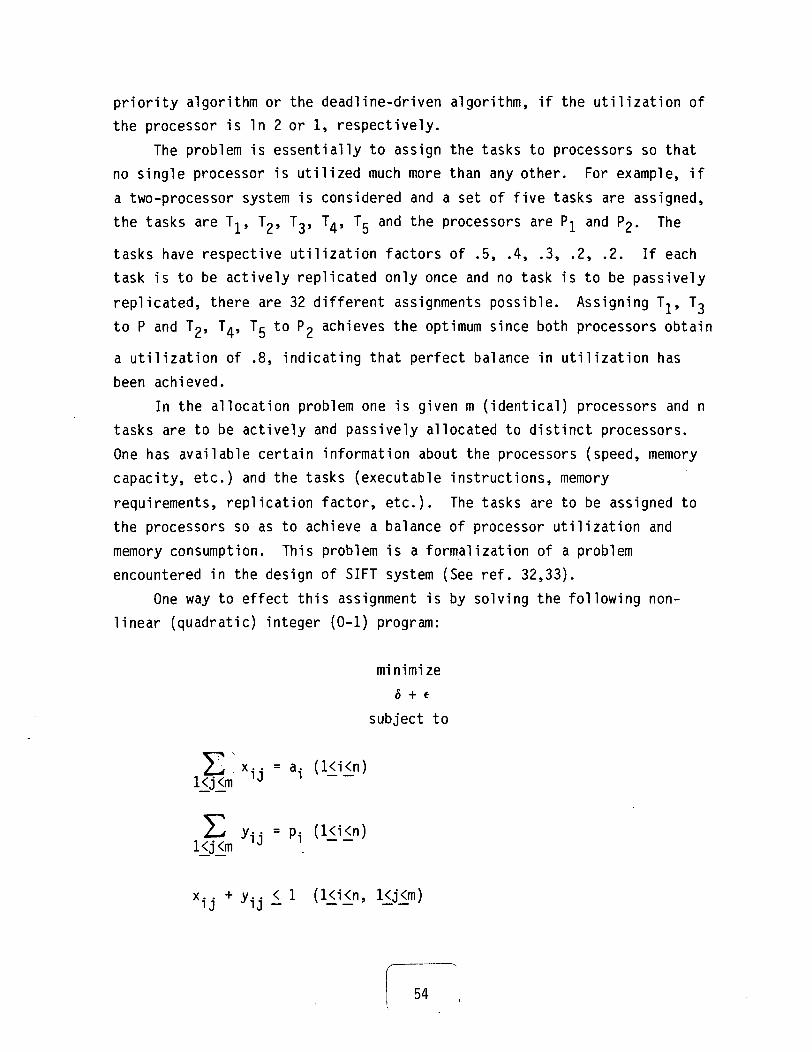
In the allocation problem one is given m (identical) processors and ntasks are to be actively and passively allocated to distinct processors.One has available certain information about the processors (speed, memorycapacity, etc.) and the tasks (executable instructions, memory
requirements, replication factor, etc.). The tasks are to be assigned tothe processors so as to achieve a balance of processor utilization andmemory consumption. This problem is a formalization of a problemencountered in the design of SIFT system (See ref. 32,33).
One way to effect this assignment is by solving the following non-linear (quadratic) integer (0-1) program:
minimize6 + e
subject to
y1n- = PKjXm IJ
U + y1d 11 (1111".
54

x . .U . < f.Ki<n 1J 1J ~ J
Ki<n
x..., y... *{0,1} (Ki<n, Kj<m)
The symbols are explained:
U.. = L/T.R. (KKn, KjXm) task i's utilization ofJ J processor j
V,- = E (x,-,- + y-iiJM,- (Kj<m) processor j's memory loading0 l<i<n 1J J
_ _ ^ - r\
6 = E ( E xiiUT,- - E E x.^-./m) variance in processorKj<m KKn J J Kl<m Kk<n ' utilization
« = E (V. - E V./m) variance in processor memory loadingKjXm J Kk<m
1 if task i is actively assignedto processor j
0 otherwise
1 if task i is passively assignedto processor j
0 otherwise
a. (Ki_<ri) = number of times task i is to be actively replicated
P-j (iXiXn) = number of times task i is to be passively replicated
L (Ki<n) = number of instructions to be executed by task iI __ —
per iteration
Kj<rn) =
55

I (ICKn) = iteration period for task i
R. (l<jXm) = speed (in instructions per second) of processor jJ
f. (l<jXm) = scheduling constant for processor j (e.g., In 2)J
M. (KiXn) = memory required by task i
C. (KjXm) = memory capacity of processor jJ
There are many possible reasons to achieve a balanced loading of theprocessors and memories:
1) The effective failure rate of a processor may be related to itsload (utilization). In a system with otherwise homogeneous processors onewill want to equalize their effective failure rates.
2) The time to reconfigure the tasks assigned to a processing unitupon its failure will certainly depend upon its loading. Since which unitwill fail first is not known ahead of time, the reconfiguration time isminimized by equal (or nearly equal) loading.
3) Since, in general, many tasks are assigned to a processor, queue-ing for its service will take place. It is a well known result of queueingtheory that the startup delay for tasks ("waiting time") is a highly non-linear function of server utilization. Clearly, one would not want any oneprocessor heavily utilized, thus creating nonacceptable startup delays fortasks assigned to it.
For convenience, the problem discussed above will be referred to asthe processor utilization and memory balancing problem (PUMBP). PUMBP re-quires the optimization of a nonlinear objective function with decisionvariables that take on zero-one values and are subject to linear con-straints. In practice, PUMBP may take up to 200 decision variables and 150constraining inequalities. There is a strong reason to believe that suchan instance of PUMBP would defy solution by traditional methods (e.g., im-plicit enumeration, branch and bound). For instance, all known algorithms
56
for the quadratic assignment problem blow up with about a dozen decision
variables.
One alternative is to try to reduce this computational burden. Tothis end, a variant of the PUMBP will be considered.
This new problem is motivated by the fact that in today's technology,memory is plentiful and inexpensive. In contrast, processor time is at a
premium. Therefore, in the new problem those decisions affecting memoryloading will be ignored and processor utilization will be the primary con-
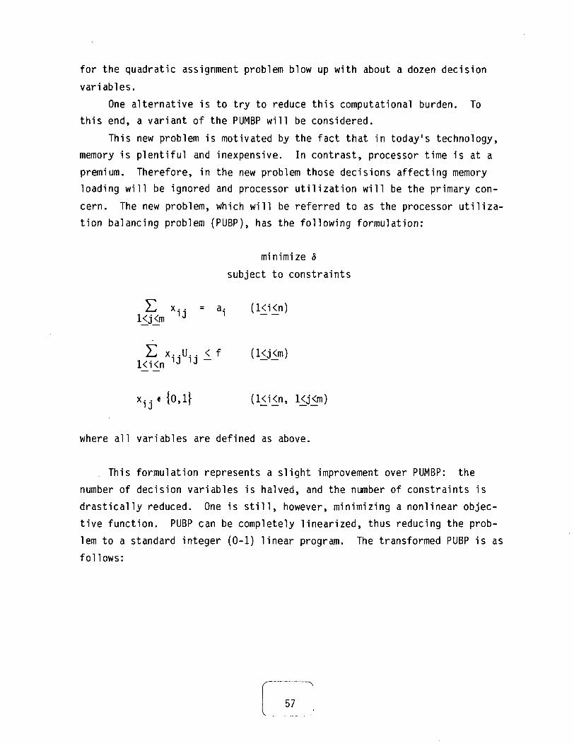
cern. The new problem, which will be referred to as the processor utilization balancing problem (PUBP), has the following formulation:
minimize 5
subject to constraints
- = a- (Ki<n)1J n
E x..U . <f (KjXm)Ki<n 1J 1J
1 .
where all variables are defined as above.
This formulation represents a slight improvement over PUMBP: the
number of decision variables is halved, and the number of constraints is
drastically reduced. One is still, however, minimizing a nonlinear objec-
tive function. PUBP can be completely linearized, thus reducing the prob-
lem to a standard integer (0-1) linear program. The transformed PUBP is as
follows:
57

minimize E( E x^ n - iD^ i - E2<j<m KiXn 1J"i 1J l<k<n
subject to the constraints
= a
E xnuu il i < n u U
xkiUkiKk<n kj kj
x, . e{0, l (Ki<n, Kj<m)' J
Observe that the objective function simplifies to
since the intermediate values of j mutually cancel each other. Thus, inthis second problem an attempt was made to minimize the (statistical) rangeof the processors' utilization factors, whereas in the first problem anattempt was made to minimize the variance of the processors' utilizationfactors. Both range and variance are measures of statistical dispersion,
although variance is generally considered the superior measure. Withstronger conditions on the problem structure, however, it may be possibleto find an assignment that minimizes variance by minimizing range, thelatter procedure being easier to perform.
Using well-known solution techniques for zero-one programming, it maybe possible to efficiently solve the above class of problems (See ref.5,20,28,31).
3.1.2.2 Heuristic approach to the task allocation problem: In their
pure forms PUMBP and PUBP seek to find optimal solutions. Solving theseproblems to optimal ity may not be possible in all cases without expending
58
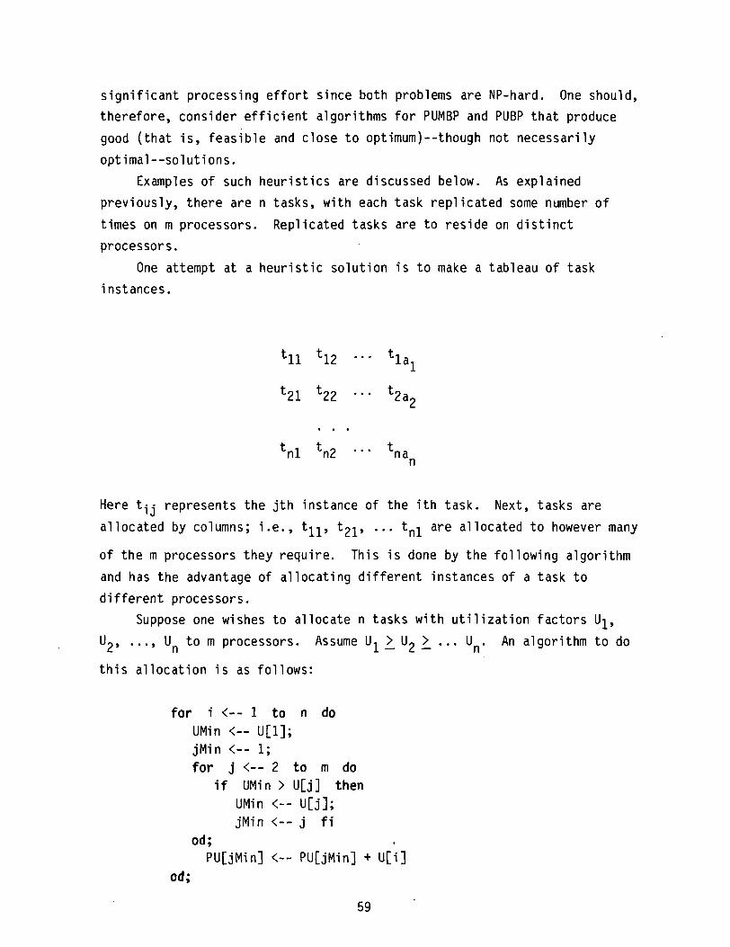
significant processing effort since both problems are NP-hard. One should,therefore, consider efficient algorithms for PUMBP and PUBP that producegood (that is, feasible and close to optimum)--though not necessarily
optimal—solutions.Examples of such heuristics are discussed below. As explained
previously, there are n tasks, with each task replicated some number oftimes on m processors. Replicated tasks are to reside on distinctprocessors.
One attempt at a heuristic solution is to make a tableau of taskinstances.
tll t!2 ••• tla1
t21 t22 ... t2a
Here t^,- represents the jth instance of the ith task. Next, tasks areallocated by columns; i.e., t^, t2}, ... tp^ are allocated to however many
of the m processors they require. This is done by the following algorithmand has the advantage of allocating different instances of a task todifferent processors.
Suppose one wishes to allocate n tasks with utilization factors Uj,Up, ..., U to m processors. Assume U, >_ U2 >_ ... U . An algorithm to do
this allocation is as follows:
for i <-- 1 to n doUMin <— U[l];jMin <— 1;for j <-- 2 to m do
if UMin > U[j] thenUMin <— U[j];jMin <-- j fi
od;PU[jMin] <-- PU[jMin] + U[1]
od;
59
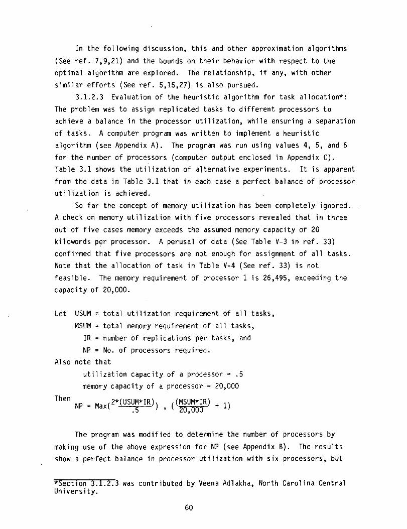
In the following discussion, this and other approximation algorithms
(See ref. 7,9,21) and the bounds on their behavior with respect to theoptimal algorithm are explored. The relationship, if any, with othersimilar efforts (See ref. 5,15,27) is also pursued.
3.1.2.3 Evaluation of the heuristic algorithm for task allocation*:The problem was to assign replicated tasks to different processors toachieve a balance in the processor utilization, while ensuring a separationof tasks. A computer program was written to implement a heuristicalgorithm (see Appendix A). The program was run using values 4, 5, and 6for the number of processors (computer output enclosed in Appendix C).Table 3.1 shows the utilization of alternative experiments. It is apparentfrom the data in Table 3.1 that in each case a perfect balance of processorutilization is achieved.
So far the concept of memory utilization has been completely ignored.A check on memory utilization with five processors revealed that in three
out of five cases memory exceeds the assumed memory capacity of 20kilowords per processor. A perusal of data (See Table V-3 in ref. 33)confirmed that five processors are not enough for assignment of all tasks.Note that the allocation of task in Table V-4 (See ref. 33) is not
feasible. The memory requirement of processor 1 is 26,495, exceeding thecapacity of 20,000.
Let USUM = total utilization requirement of all tasks,
MSUM = total memory requirement of all tasks,IR = number of replications per tasks, andNP = No. of processors required.
Also note thatutilization capacity of a processor = .5memory capacity of a processor = 20,000
Then MP = M,..,2*(USUM*IR),20,000
The program was modified to determine the number of processors by
making use of the above expression for NP (see Appendix B). The resultsshow a perfect balance in processor utilization with six processors, but
*Section 3.1.2.3 was contributed by Veena Adlakha, North Carolina CentralUniversity.
60

again memory exceeds the processor capacity of 20 kilowords in three cases
(see Appendix C).
The program was further modified to place a check on memory at each
step. To reiterate, the program arranges the processors in ascending order
in terms of accumulated processor utilization. Before going down the listand assigning replications of a task, the program checks the total memory,
if the current task is assigned to that processor. If the total memoryexceeds the memory capacity of 20,000, the possiblity of assigning the task
to the next processor is explored. Table 3.2 presents the results of thisexperiment (see Appendix C). It is clearly established that a balance in
both processor memory and processor utilization is achieved.3.1.2.4 Performance guarantees for a restricted task allocation
problem: In this case, the following problem is considered. There are mprocessors and n tasks. All processors are identical, and all tasks have
known utilizations ui (KKn). One desires to assign each task to twoseparate processors in such a way that the statistical variance of the
processors' utilization is minimized. (The utilization of a processor isdefined to be the sum of the utilizations of all tasks assigned to the
processor.) This subproblem of PUBP will be referred to as the BALANCE
problem.
The problem described above arises in connection with a real-lifeproblem in the design of fault-tolerant real-time computing systems. The
scenario is a fault-tolerant system in which two copies of a process areconcurrently executing on different processors. Thus a single faulty
processor may be identified by voting on the processors' results.*The problem can be made mathematically precise as follows:
1 \~^Minimize •=:/.(m L
subject to the constraints
„ :ij = 2 (KKn)j
x. . e {0,1} (KKn, KjXm)
* I he results presented are valid for processes with arbitrary replicationfactors, but the proofs are more complicated.
61

Table 3.1Processor Utilization
Number of ProcessorsProcessor 4 5 6
1 .420 .321 .268
2 .420 .322 .268
3 .420 .321 .268
4 .420 .322 .268
5 -- .322 .268
6 -- -- .268
62
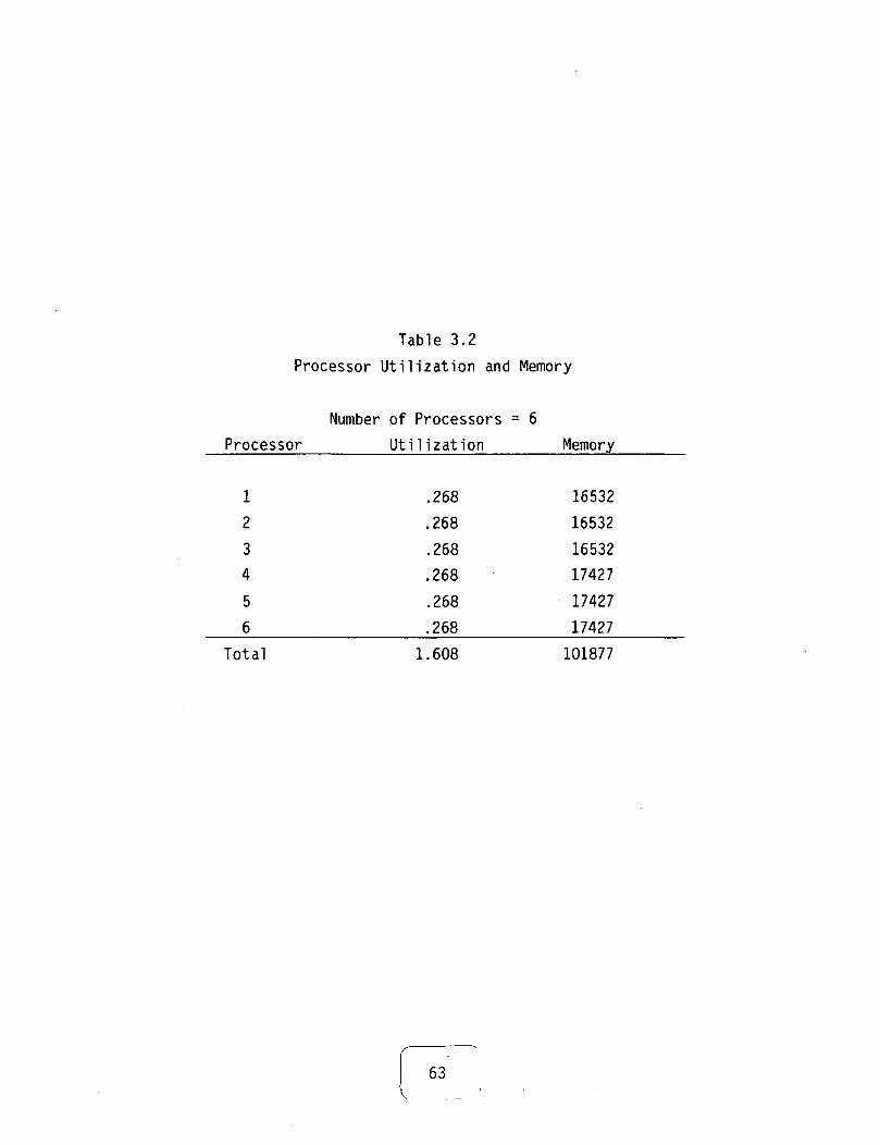
Table 3.2
Processor Utilization and Memory
ProcessorNumber of Processors = 6
Utilization Memory
1
2
34
5
6
Total
.268
.268
.268
.268
.268
.268
1.608
16532
16532
1653217427
17427
17427
101877
63
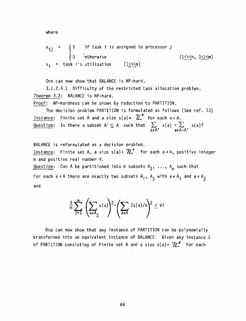
where
X.. = 1 if task i is assigned to processor j
0 -otherwise (ICKn, KjXm)u- = task i's utilization (Ki<n)
I """* ~~" *
One can now show that BALANCE is NP-hard.3.1.2.4.1 Difficulty of the restricted task allocation problem.
Theorem 3.2: BALANCE is NP-hard.Proof: NP-hardness can be shown by reduction to PARTITION.
The decision problem PARTITION is formulated as follows (See ref. 13)Instance: Finite set A and a size s(a)« 1L for each a « A.Question: Is there a subset A' c A such that £] s(a) = zL s(a)?
a«A' a«A-A'
BALANCE is reformulated as a decision problem.
Instance: Finite set A, a size s(a)« 7Z- for each a « A, positive integerm and positive real number V.Question: Can A be partitioned into m subsets A,, ..., A such that
for each a«A there are exactly two subsets A^ , A. with a « A., and a < A .
and
One can now show that any instance of PARTITION can be polynomiallytransformed into an equivalent instance of BALANCE. Given any instance Iof PARTITION consisting of finite set A and a size s(a)e 7// for each
64
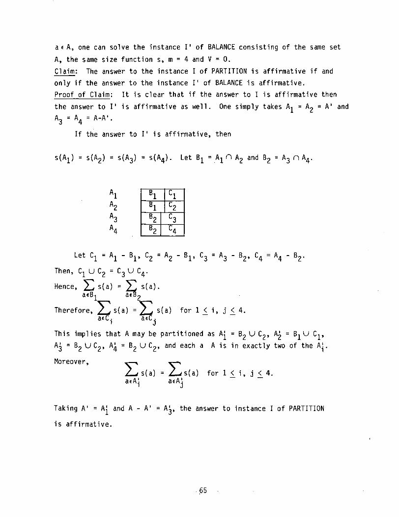
a « A , one can solve the instance I1 of BALANCE consisting of the same set
A, the same size function s, m = 4 and V = 0.
Claim: The answer to the instance I of PARTITION is affirmative if and
only if the answer to the instance I1 of BALANCE is affirmative.Proof of Claim: It is clear that if the answer to I is affirmative then
the answer to I' is affirmative as well. One simply takes A^ = A2 = A1 andA3 = A4 = A-A'.
If the answer to I1 is affirmative, then
s(A1) = s(A2) = s(A3) = s(A4). Let BI = t\± n A2 and B2 = A3 n A4.
Then, C, U C~ = C, U C,.J. L- O ^
"" -NHence, / s(a) = / J s(a).a«B^ a«B2
Therefore, / j s(a) = / ^ s(a) for 1 <_ i, j <_ 4.aeCi ae .
This implies that A may be partitioned as A| = B2 U C2, A2' = B^ U C^,
A^ = B2 U C2, A4 = B2 U C2, and each a A is in exactly two of the Ai
Moreover, - ^
2-^s(a) = 2-/s(a) f o r l < ^ i , j < 4 .
»jaeA'.'
Taking A1 = Aj^ and A - A1 = A3, the answer to instance I of PARTITION
is affirmative.
65

3.1.2.4.2. An approximation algorithm and its performance guarantee.The balance problem is NP-hard. Thus one should to consider approxi-
mation algorithms with efficient execution times. The following algorithmis one example. It will be referred to as algorithm "A".
0) i <-- 1.
1) Find the two least utilized processors (of lowest indices) andassign task i to them (twice).
2) i <— i + 1. If i > n then stop or else go to (1).
Here the assumption is that u^ >_ ,.. >^ un.
Definition 3.1: Let S be a set of numbers. Definenin S = min (S - {min S)). This is known as the "next minimum."N.B. nin T _< nin S, T _< S.
Lemma 3.1: Suppose that algorithm A is applied to tasks with utilizationsul 2l ••• >. un on m Processors. Let q-p ..., qm be the resulting processorutilizations. Then max (q.-l - nin {q-} < u,, where k is the last task
j J ~assigned by A to the maximally utilized processor.
Proof: Suppose that q, = max {q.} and one copy of task k is assigned toj J
processor 1, algorithm A assigns task k to the two least utilizedprocessors. Assume that task k was assigned to processors 1, I1. Let p,,
..., pm be the accumulated processor utilizations just immediately beforetask k was assigned to processors 1, 1' by algorithm A. Then
p-i + UK = q-i = max {q.l . Also, p-| _< nin (p.} , since processor 1 was oneJ J
of the two least utilized processors at the time task k was being assigned.
Moreover, p. <a. (l<j<m). Therefore p-, _< nin (p.K nin (q.) . Hence,J J i j J j Jrewriting p, as max (q.) - u. , results in max {q.}- u. <_ nin (q.) , and
1 j J j J K j J
the lemma is proved.
Definition 3.2: Let q = (qp ..., qm) and p = (pp ..., p ) be two sequences
66

such that q., p. _> oA ^q. =^ p. and max {q.} _< 2nin {q.} . DefineJ J £—J J ^^~ J -j J -j J
j j
K(m) = lubt^(q.)2/ V(P-i)2 >. Also define K = lub;{K(m)} .L*t J Z^ J mq>p * m
j J
Lemma 3.2: Suppose that there are n tasks with utilizations u,, ..., uwhich are to be legally (i.e., two copies of each task are assigned to dis-
tinct processors) assigned to m processors. Let q^, ..., q be the proces-sor utilizations resulting from algorithm A. Let qt, ..., q* be the
processor utilizations resulting from optimal algorithm 0. Then
Proof: Let q-, = max {q-}» and suppose that task k was the last taski
assigned by algorithm A to processor 1. Also assume that task k was
assigned (redundantly) to processor T. Let p^, ..., p be the processorutilizations immediately before task k was assigned. We have two cases.
Case 1: p-| ^ 0. Then 0 < p-| <_ p- > 0 (l<jXm, j ^ I 1), since proc-essors 1 and 1' were the two least utilized processors prior to the
assignment of task k. Thus p. > u,, (Kj<m, jVl'h since each of theseJ — *
processors had a task (of utilization at least u. ) already assigned to it-recall that p. > 0 (KjXm, j/11). Therefore nin {q.} >_ u, because
J •; J K '- -q. > p. and u, < min {q.} < nin {q.} (since u. < p- < q- for 1 < j < m,J ~ J K — • /11 j — • j K j j
J>"1 .')j"7T Clearly V^q • = V^q*- Hence, by Lemma 3.1,
max {q.} < nin {q.} + u, < 2nin {q.} .j J ~ j J k~ j J
Therefore,
67

Case 2: p, = 0. Then p. = 0 (j'2.1) and p. = u, (j<l) because q, = u. isI J J K I K
maximal. Find the smallest number t such that there is a processor s which
has at least two tasks assigned to it and max J q . l = q . For example seei~>t ' J > s
Figure 3.2. J-
There are two subcases of case 2.Subcase 2.1; No such t exists. Then all processors have l.ess,than:two tasks
assigned to them. In this case A has produced an optimal assignment and
Subcase 2.2; Such a t exists. Suppose task r was the last task assignedto processor s by algorithm A. Then, by Lemma 3.1,
max |q-l - nin J q. I < u . Also, u < nin jq. I . Hence,' J ' J ' ~ r r ~ ' -J '
max Jq, t nin jq. | + u < 2nin {q.}.j_>t J j>t J J2*
The next step is to perform a cost-preserving transformation on the\
optimal assignment.
Claim: The optimal assignment resulting in processor utilizations qt, ...,
q* can be transformed into an (not necessarily legal, i.e., two copies of a
task may be assigned to the same processor) assignment with processorutilizations qj, ..., q' such that
2 ~"V 2
J J J J
and
(1 < j < t).
68

123456789101112
t = 7 s = 9
Figure 3.2. Example of the construction of t and s,
69

Proof of Claim: The transformation is as follows:
1) Do until none of the tasks 1, 2, ..., p[• are co-assigned to
the same processor: If two of tasks 1, 2, ..., \—?r\ are co-assigned toa processor, then place the smaller task on the least utilized processor
that has assigned to it none of the tasks 1, 2 ~~2~ ' This step is
always possible if two of tasks 1, 2, ..., t-1 are co-assigned to a
processor. The transformation will never increase the cost of the assign-
ment. (See Figure 3.3.)2) Assume that now the processors have been renumbered so that task j
is assigned to processors 2j-l and 2j (1 <_ j _< |t/2j). (See Figure 3.4.)
Note that none of the tasks 1, 2, ..., —^— are assigned to processors
. , . , ft-llt, . . ., m, and if 1 , then tasks and J,2 are assigned
-1< i'2 <.to different processors. Now, if tasks i^ and i~ (1 <. ii _<
are assigned to processor j, (IXjXt), then find a minimally utilized
processor among t, ..., m (say j~). Then q'. < u. (by construction oft . • j2- T!t). Task \2 can be removed from processor j^ and assigned to processor
J2 with no cost increase. (See Figure 3.5.)
ft-flStep (1) can be applied until each of tasks 1, 2, ...,
assigned to a separate processor. Then step (2) can be applied until each
(instance) of tasks t-1 + 1, ..., n is assigned to one of the processors
t, ..., m. The ultimate assignment is as in Figure 3.6 (after renumber-
ing).
Let q']_, .., q'm denote the processor utilizations in thetransformed assignment. The transformed assignment has cost no more than
the optimal legal assignment; i .e. ,
In both the transformed assignment and the assignment resulting from
algorithm A, task i is assigned to processors 2i-l and 2i (1 j< i £ [t/2j ) .
Therefore, q, = q'. (l<j<t), andJ J
70

1 1 j-L < J2 < t contains no task 1, 2, ...,
transformed to ...
so cost doesnot increase
Figure 3.3. Cost-preserving transformation of the optimalassignment by step (1).
71

b«J
m
Figure 3.4. Assignment after applicationof step (1) and renumbering.
72

transformed to ...
\• • • \
so cost doesnot increase
Figure 3.5. Cost-preserving transformation of theoptimal assignment by step (2).
73

t-1
t
m
only tasksft-1/2] +1, ..., nare assigned to theseprocessors
Figure 3.6. Final assignment after transformation bysteps (1) and (2). The transformed assignmentcosts no more than the optimal assignment.
74
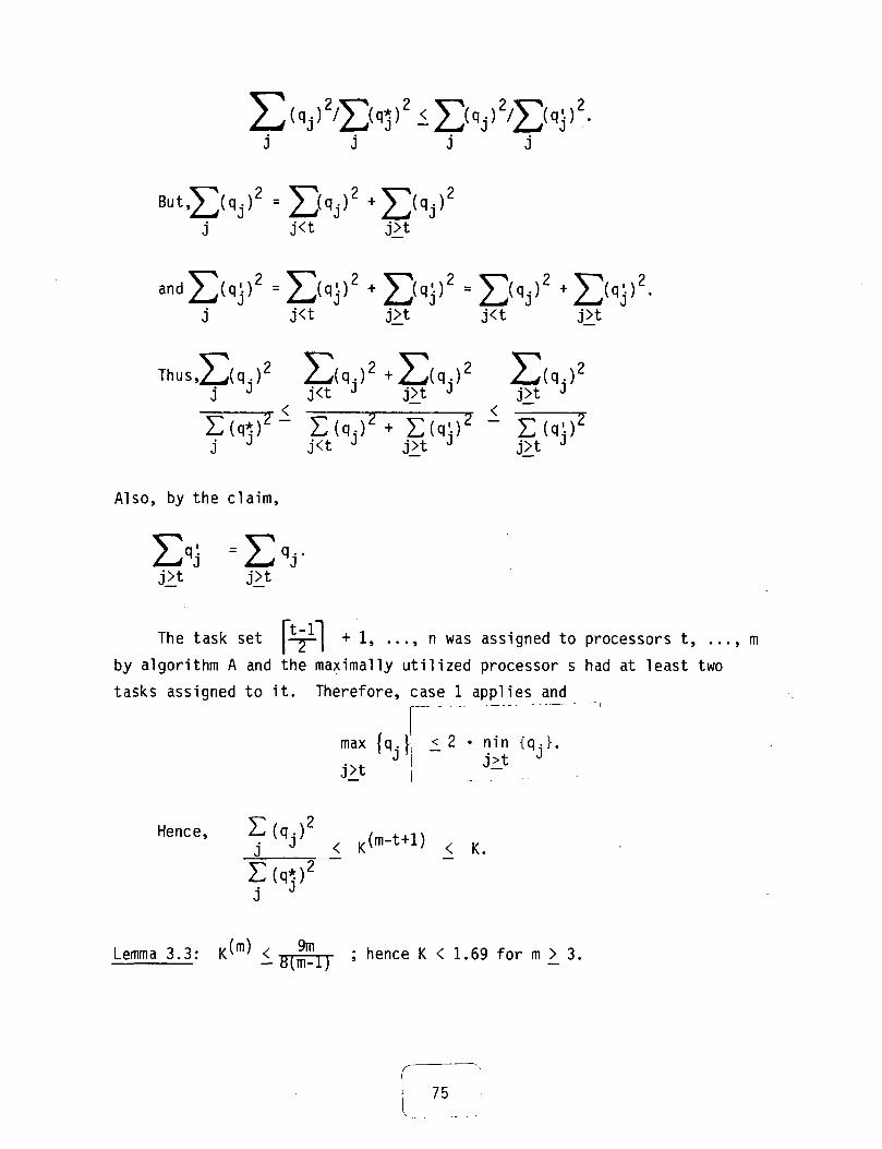
j<t JH
E(2(q,)jx
Also, by the claim,
The task set — i— +1, ..., n was assigned to processors t, . . . , mby algorithm A and the maximally utilized processor s had at least twotasks assigned to it. Therefore, case 1 applies and
max {q. |j £ 2 • nin {q,}.J ' J-*
Hence, (q,) (m_t+1)j J < Klm r L) < K.
Lemma 3.3: IOm' < „,-"",. ; hence K < 1.69 for m > 3.
75
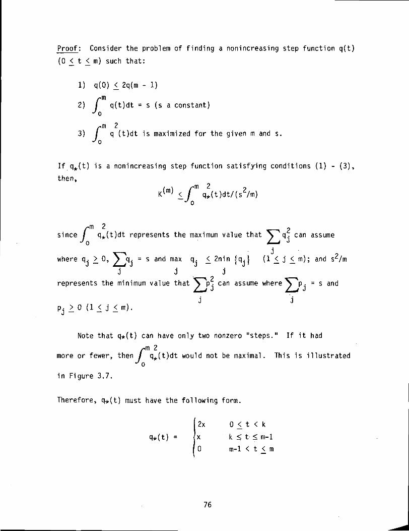
Proof: Consider the problem of finding a nonincreasing step function q(t)
(0 _< t <^ m) such that:
1) q(0) <
/
mq(t)dt = s (s a constant)
ify
3) / q (t)dt is maximized for the given m and s.J n
If q*(t) is a nonincreasing step function satisfying conditions (1) - (3),
then,/ \ /-
KimJ <J•m 2
o
/
m 2 ^ £q*(t)dt represents the maximum value that \ ^ q. can assume
/ j J
2c
•'o
V^ J' ' 9where q. >. 0, > q, = s and max q. _< 2nin |q. 1 (1 <_ j £ m); and s^/mJ A^^^ J J J
j J J• ^
represents the minimum value that \ ^p. can assume where \ Ap. = s and
p. >0 (1 < j < m ) .
Note that q*(t) can have only two nonzero "steps." If it had
/
m 2q..(t)dt would not be maximal. This is illustrated
u
in Figure 3.7.
Therefore, q*(t) must have the following form.
q*(t) =2x 0 _< t < k
x k < t < m-10 m-1 < t < m
76

q*(t)
one step
m-1
can be transformed to better
q**(t)
m-1
/•m p ^J q**(t)dt > J q*(t)dt
Figure 3.7. q*(t) cannot have one step.
77

q*(t)
three-or-more step
m-1
q* can be transformed to better
q**(t)
m-1
'PI 2l*(t)dt
Figure 3.7 (continued). q*(t) cannot have three or more steps.
78

Thus, s = 2xk + x(m - 1 - k) and k = s/x - m + 1. So
"2q*(t)dt = 4x2(s/x - m + 1) + x2(2m - s/x - 2)
= 3sx + 2x2 - 2mx2.
This attains a maximum of
w h e n x = 3 s
8m - 8 "'""' 4m - 4'
Hence, K^ < -| . -=r -r .— o m - i
For the PUBP the performance of approximation algorithms is compared
to optimal algorithms. Simply comparing the statistical variance is notsufficient since one should normally expect the variance allowances todiffer for differing task sets. Therefore a.measure akin.vto .thecoefficient of variation will be used. Given an approximate assignment
(x-jj) and an optimal assignment (x'jj) the relative costs arecompared as follows:
Theorem 3.1: Suppose that there are n tasks with utilizations u^, ...,
un which are to be legally (i.e., two copies of each task are assigned todistinct processors) assigned to m processors. Let q^, ..., qm be the
processor utilizations resulting from algorithm A. Let qj q* be the
79

VA =
processor utilizations resulting frpm optimal algorithm 0. Let
1 X~~* 2 // 2 X~^ \2= -—- > q. /(-:::- / u. \ denote the relative variation in processor
J *
utilization under the approximate assignment A. Let
VQ = -i- N A(q^) /( -_— \ ^ u. | denote the relative variation in
J ' iprocessor utilization under the optimal algorithm 0. Then
AdVA/VO< i <..*)^n- < 1.69 (m > 3)
Hence, the approximation algorithm is always less than 69% off optimum.
Proof: Note that VA/VQ = jf. I ']T(q*)2. '
j. / jBut for m = 2, algorithm A produces optimal assignments. Therefore, by
.3, VA/VQ 1 sfm IT < 1'69 for m 1 3» and VV0 = 1 for m = 2Lemma 3.
3.1.3 Task allocation for reliability maximization*. - A function
f(_x) of a vector argument _x = (x^, x2, ..., xn) is said to be symmetric iffor any permutation y_ = (y,, y^, ..., y ) of £» f(x_) = f(y.)« A function
f(_x_) is said to be concave if
Af(x_(1)) + (1 -x)f(_x(2)) <_f (\x.(1) + (1 - A)_x(2)).
Definition of a convex function is obtained by reversing the inequality
above. A set C of points is said to be convex if for
C,\x(1) + (l-X)x^2) «C for X> 0.— —
^Section 3.1.3 was contributed by Kishor Trivedi, Duke University.
80
Theorem 3.2: A symmetric concave function f(xj over a symmetric convexspace is maximized by equalizing all of its arguments.
Proof: Assume that there is a two-dimensional feasible space forconvenience, although the argument is easily generalized. The proofproceeds by contradiction.
Assume that the optimal point is (x,y) where x ^ y. Since thefeasible space is symmetric, then (y,x) is also in it. Furthermore, sincethe feasible space is convex, any point on the line joining the two points
is also feasible. In particular, (- i , -) is feasible. By symmetry of
f(_x), f(x,y) = f(y,x) is the maximal value, but by concavity of f,
> f(x.y) + lf(x,y) = f(x,y)
which implies that (-r^ r) is also an optimum.
Thus, if one assumes that the system reliability is a concave functionof detection latencies, for instance, then clearly it being symmetric, thereliability is maximized by equalizing detection latencies. Similarly,reliability is maximized by equalizing reconfiguration times and so on.
Given enough time, concavity of reliability may also be established.
3.2 Discussion of the Role of Software Design*
3.2.1 Introduction to classical engineering design methodology. -
This section discusses the elements of classical engineering designmethodology with particular reference to software engineering. It assumesa basic familiarity with the problems of software engineering.
*Section 3.2 was contributed by Thomas Alspaugh, Jr., IBM, Research
Triangle Park.
81

The term "methodology" is often considered a buzzword. According toWebster, a methodology is "a body of methods, rules, and postulates employ-ed by a discipline". Sage (See ref. 29) narrows it to "a set of tools, aset of proposed activities for problem solution, and a set of relationsamong the tools and activities". These are very broad, high-leveldefinitions; indeed, methodologies themselves are difficult to expressexcept in broad, high-level terms. They are so abstract that a trueunderstanding of them requires a consideration of the concrete applicationwhich inspired them.
Engineering solutions can be applied to a certain restricted class ofproblems that can be adequately expressed in explicit, concrete, andquantitative terms. Such solutions are characterized by predictablebehavior which can be quantified and verified. The creation of such solu-tions is constrained by the limited capacity to deal with complex ideas orconsider all the ramifications of complex interactions. The methodologydeals with these issues and problems.
Nearly everyone has had the experience of apprehending and solving asimple everyday engineering problem almost at one stroke, with no consciouseffort. The problem was apprehended intuitively, synthesis of the solutionoccurred unconsciously, and understanding of the situation was so intimatethat it was a foregone conclusion that the realization of the solutionwould meet the need completely. But most problems are not so tractable.The methodology helps one to solve problems by conscious effort whiletrying to attain the unity and integrity that characterize the correctintuitive solution.
3.2.2 The classical engineering design methodology. - The methodologyconsists of a number of components: abstraction, the "black box", specifi-cations and testing, the design process, iterative convergence, recursivedecomposition, documentation, and pilot operation. Each component is con-sidered below.
3.2.2.1 Abstraction: Abstraction is a powerful concept that perme-ates the engineering design methodology. The process of abstractionconsists of conceptually separating the important characteristics of a
82

situation or object from a mass of unimportant information. The character-istics that were abstracted form a model or abstraction that can stand forthe situation or object itself to a certain extent. This abstraction canbe studied and manipulated instead of the complex thing from which it wasabstracted, and if the abstracted characteristics are well chosen theresults are applicable to the thing itself. This is a powerful techniquefor dealing with complex things and ideas.
Three examples of the use of abstraction in the creation of engineer-ing solutions follow. In considering the problem, certain aspects of itwill be important and others less so. Also, it may be useful to considersome characteristics of the problem in terms of mathematics or some othermental model rather than in the terms of the problem itself, thus ignoringsome aspects of those characteristics. The solution itself will have manyproperties irrelevant to the problem it solves, or it may be only anapproximate solution, though close enough for practical purposes.
3.2.2.2 The black box: The concept of the black box is a particular-ly important example of abstraction. A black box is a system whose innerworkings are completely invisible. Its externally visible behavior can bedescribed completely and concisely. Its internal structure may be, andprobably is, much more complex, but this complexity need not be consideredin using the black box. An engineering solution that can be conceived ofas a black box is more useful than one that cannot. Such a system isallowed more flexibility in its internal workings, since only a smallsubset of its characteristics are constrained. It is easier to think aboutand use, since its behavior can be described more abstractly and moreconcisely. It is easier to reuse later in another problem, since it doesnot require a large investment of time to understand how it behaves.
3.2.2.3 Specifications and testing: The technique of specificationsand testing arises from the nature of engineering, which considers thingsin terms of quantifiable physical characteristics. Thus, an existing ordesired engineering solution can be adequately described in such terms. Anabstraction of a solution or a set of solutions can be so expressed; if theabstraction contains precisely the properties that a satisfactory solution
C83
must have, then its description constitutes the specifications for thesolution, the requirements which a solution must meet in order to besatisfactory. The properties of a candidate solution can be tested andcompared with the specifications to decide if the candidate is asatisfactory solution.
3.2.2.4 The design process: The design process is a sequence ofsteps whose goal is to develop a solution for a complex problem. Theprocess is arranged to encourage the same integrity that occurs in the case
of intuitive solutions to simple problems. The steps of the process aredepicted in Figure 3.8. They are:
1. Problem definition. The problem is explored and its importantcharacteristics are abstracted. No reference is made to possiblesolutions; the problem is considered in its own terms. Objectivesand criteria for solutions are developed and the worth of having asolution (or the cost of not having a solution) is estimated.
2. Requirements. The statement of the problem is recast in terms ofengineering. The requirements that a candidate solution will haveto meet in order to be acceptable are developed. Still noreference is made to specific solutions.
3. Design synthesis. A design for a system that will meet therequirements is synthesized.
4. Realization. The design is realized.
5. Design test. The realization of the design is tested to ensurethat it meets the requirements determined in the second step.
6. Requirements test. The realization of the design, which has nowJjeen established as an embodiment of the requirements, is tested"in the context of the problem to ensure that the requirements meetthe definition of the problem and that the definition of theproblem is accurate.
The integrity of the process is verified by the testing steps.Divergence can occur at each point at which a new abstraction is developed:
problem definition, establishment of requirements, design synthesis; and atthe point at which an abstraction is realized: design realization. The
process may be viewed as a chain of abstractions leading from the problemto its concrete solution. If each abstraction is accurate and well chosen
84
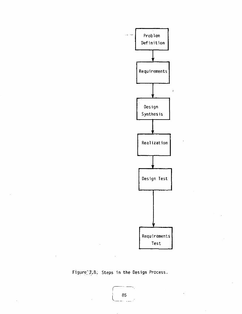
ProblemDefinition
Requirements
Design
Synthesis
i'.
Realization
Design Test
Requirements
Test
Fi;gure'i3.8. Steps in the Design Process,
85

and if the realization correctly reflects the final abstraction, then thesolution will necessarily meet the needs of the problem. The testingensures that each link in the chain is firmly joined to what comes before.
3.2.2.5 Iterative convergence: Iterative convergence refers to thetrial-and-error process by which the abstractions in the design process areimproved. The limitations of our mental capacity make it unlikely thatabstractions will be adequate from the start. The testing steps may revealfaulty abstractions and provide a means for pinpointing their shortcomings.The design sequence is then followed again, starting from the improved
abstraction (Figure 3.9).3.2.2.6 Recursive decomposition: Nearly all problems are too large
to solve as a whole. The required solution would be too complex to beadequately understood. In such cases the solution can be analyzed as thecombination of several black boxes, each of which is then considered as asubproblem. The subproblems are treated precisely as any other problemneeding an engineering solution; each subproblem is analyzed, requirementsare generated, and a subsolution is designed, realized, and tested. If
these subproblems are also too large, they can be similarly decomposed in arecursive manner until manageable problems are obtained. The solution tothe original problem is obtained by recursively assembling all thesubsolutions.
The correctness of the abstraction involved in the decomposition istested when the subsolutions have been implemented by combining them andtesting that the combination meets the requirements established for thesolution.
3.2.2.7 Documentation: Documentation is an important part of thecreation of an engineering solution in that it provides information needed
by the users and maintainers of the solution. Less obvious is its value tothe creators of the solution. The structure of the documentation directs
the thought of the writer, and if the structure of the documentation iswell chosen, the writer will be assisted in relating the important issues
of the solution. The act of writing itself forces the thorough consider-ation of what is being written, and questions that can be glossed over in
86
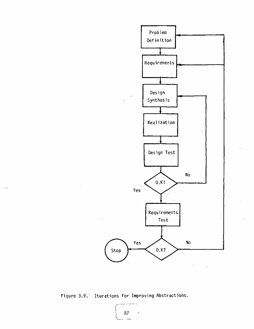
Problem
Definition
Requirements
Design
Synthesis
1Realization
Design Test
Yes
No
RequirementsTest
No
Figure 3.9. Iterations for Improving Abstractions.
87

one's mind become painfully obvious when they are put on paper. Brooks
(See ref. 4) also points out that the management of the creation of anengineering solution revolves around a relatively small body of informationconcerning the system, and the writing down and dissemination of thisinformation is a crucial part of the managing task.
3.2.2.8 Pilot operation: The term "pilot operation" refers to asmall-scale test solution used to gain knowledge and experience that willbe useful in the creation of a large and expensive solution. The pilotoperation risks a relatively small investment to reduce the risk that thelarge investment for the actual solution will be wasted. Pilot operationsare useful for solutions embodying ideas that have never been tested or
that have been tested only on a much smaller scale; large changes of scalechange the relative importance of the aspects of the problem and solutionwhich must be taken into account, thus possibly invalidating theabstractions that were appropriate on a small scale.
3.2.3 Software engineering. - Certain areas of the methodology pose
special problems or are of special interest in software engineering. Theyare described below, organized by the component of the methodology with
which they are concerned.3.2.3.1 Abstraction: In Brooks' phrase, programmers work with a very
tractable medium (See ref. 4). The flexibility inherent in programmingmeans that any program is the embodiment of a large number of implicit or
explicit decisions which together define the program. It is difficult toabstract from such a large number of decisions, particularly since they mayinteract in complex ways. Also, software deals with dynamic processesthat evolve over a period of time; such processes are more difficult tothink about than the more static relations that characterize other
engineering disciplines (See ref. 11).3.2.3.2 Black box: For these same reasons, black boxes are more of a
problem in software engineering. Problems with software engineering black
boxes are usually thought of as problems in the interface, which is themanifestation of the abstraction that describes the black box. Softwareblack boxes also are less easily portable because the inputs they requiremay be difficult to abstract and understand.
88

3.2.3.3 Specification and test: Software specifications commonlyspecify both too little, and in one sense, too much. The large number ofimportant decisions makes it difficult to cover all the important decisionswhen making specifications; this leads to the ad hoc making of designdecisions by the implementers, who usually have no overview of the solutionand cannot be relied upon to choose correctly. In another sense,specifications often specify too much, in that they unduly restrict theimplementation (See ref. 23).
3.2.3.4 The design process: Several parts of the design process areof particular concern.
When considering a problem to be solved by software, it is very tempt-ing to define the problem itself by specifying to some level of detail apossible solution. Most software engineers find it easier to think insoftware terms than in terms of a specific problem.
Two aspects of the process of synthesizing the design of a solutionare of special concern. First, it is very desirable but not easy for de-signs to reflect the natural structure of a solution. It is desirablebecause such designs are much easier to think about, but it is difficultbecause problems almost always have some aspects that are difficult toreconcile with the main characteristics. Second, solutions usually need tobe adapted to slightly different problems as time goes by, and it is desir-able to design a solution so it may be adapted easily.
Testing software is of limited value since tests can only show thepresence of errors, not their absence. The complexity of software solu-tions requires extensive tests to provide confidence that the software isreasonably free of errors. Formal proof is a tempting alternative, but ithas drawbacks also. The process of proving correctness is arduous, andalso it is all too easy to prove one thing while thinking one is provingsomething else.
3.2.3.5 Iterative convergence: The iterative process of testing,finding, and fixing problems in a software solution tends over time to makethe structure of the solution less orderly, particularly if the problemsshow up some length of time after the solution was tested and declaredaccurate. The temptation to attempt to repair the solution without takingthe time to understand it completely, together with the natural human
89
tendency to treat symptoms before the underlying problem is evident,combine to make the solution not fit its abstractions and behave in morecomplex, less predictable ways as it grows older.
3.2.3.6 Documentation: The complexity of software solutions makesthem more difficult to document. Because software is so flexible andtractable, any solution involves a large number of decisions. The amountof information that must be organized and recorded in the documentationmakes it likely that the organization of that information will not be verygood. Ideally, the documentation should be useful both as an introductionor overview for a neophyte and as a reference for a person who has at leastthe knowledge provided by the overview but not necessarily a thoroughunderstanding of the whole software system. In fact, this rarely occurs.
Parnas (See ref. 24) lists six important problems plaguing mostsoftware documentation.
1. It is obtuse in the assumptions made about the purposes andknowledge of the reader.
2. It is hard to use as a reference.
3. It is expensive to maintain.
4. It is repetitive and boring, and thus is not read attentively.
5. It uses inconsistent terminology.
6. It is written for people who know as much as the writers of thedocumentation.
The writers of most documentation try to make each piece of informa-tion understandable when looked up for reference by surrounding it with thebackground they believe it requires. This means that any particular factis likely to be recorded in many places throughout the documentation, andif the decision leading to that fact is changed a great deal of effort isrequired to revise the documentation. It also means that a person reading
the documentation will encounter many facts over and over again, probablyexpressed in exactly the same sentences and paragraphs.

3.2.4 Software engineering tools and techniques. - Certain tools and
techniques have been developed to aid in the creation of software engi-neering solutions.
3.2.4.1 A set of documents: Brooks (See ref. 4) presents a set ofdocuments intended to aid in the management of a software project. Theyconsist of: (1) the objectives—defining the problem, the goals, the
constraints and the priorities; (2) the specifications—consisting of theuser's manual for the system to be created, which he views as setting forththe requirements for the visible behavior of the system, and the internaldocumentation; (3) the schedule; (4) the budget; and (5) the space
allocation and organizational chart for the people working on the system.Parnas (See ref. 24) lists a set of documents useful in the creation
of a software system. They are: (1) the requirements for the solution;(2) secret test plans, to be concealed from the implementers of the
solution; (3) the software decomposition document; (4) the individualmodule interface documents; (5) the individual module design documents; (6)the uses/subsets document, setting forth the interdependences betweenmodules and the useful subsets of the whole system; and (7) the processstructure document, dealing with scheduling.
3.2.4.2 Formal languages: English prose is not well adapted for aprecise and unambiguous description of software systems. Many formallanguages have been developed for various aspects of software engineering,though none has been very widely used except in the specification ofprogramming languages. Two examples of formal languages which bear on thesoftware engineering design methodology are TRACES, which is used inwriting module specifications (See ref. 2), and SPECIAL, which is used inwriting more general specifications (See ref. 25).
3.2.4.3 Modularity and information hiding: The classical motivationbehind the use of black boxes is portability. Two more motivations formodularization are the splitting of the task into work assignments for asingle person or a small group so that a minimum of coordination and
communication between subtasks is needed, and the reduction of the inter-dependence of the decisions that together define the solution, so that atleast some decisions may be changed without reworking much of the solution
91
(See ref. 23). To achieve these goals, the system may be modularized usingParnas" principle of information hiding, so that every decision that islikely to change is hidden in an abstract module whose external behavioris not dependent, on the decision, and that in fact every module in thesystem depends not at all or as little as possible on the way anyparticular module is implemented.
3.2.4.4 Reference vs. statement in documentation: In computerlanguages an abstract name can be used to refer to a constant whose actualvalue is defined at precisely one place in a program. Documentationwritten analogously by using abstract names to refer to specific decisionswould be very simple to change; if the documentation was organized strictlyand simply, it would also be easy to use as a reference. Heninger et al.
(See ref. 17) have done precisely that in the complete rewriting of thevery large requirements document for the A-7 Operational Flight Program,and the result has been quite successful.
3.2.4.5 Simulation: Software engineering allows another kind ofdecomposition. A solution that would normally be a complex program runningon a simple machine can be broken down into a simpler program running on amore complex abstract machine, and a program, running on the simplemachine, which simulates the abstract machine. A well-chosen decompositionof this type can make a significant reduction in the effort required to
implement a solution.
92

4.0 CONCLUSIONS AND FURTHER WORK
This report has presented a methodology for the initial identification
and design of integrated aircraft electronic systems that are intended foruse in commercial aircraft.
The report presented a taxonomy of multiprocessor systems as a frame-work for understanding, discussing and characterizing systems. This taxon-
omy included the identification of major system design parameters. A meth-odology for estimating system behavior was also proposed. System behavior
is partially described in terms of the reliability, performance and cost ofa system. Measures for reliability, performance and cost were defined and
applied to the proposed taxonomy, and a strawman system was identified.The report also included a discussion of algorithms for and control of
fault-tolerant integrated aircraft electronic systems. Management of sys-tem resources, especially scheduling and task allocation were shown to beimportant to the reliability and performance of a fault-tolerant integratedaircraft electronic system. Formal analysis of scheduling and allocation
algorithms demonstrate the usefulness of approximation or heuristic algo-rithms. The role of software design methodologies was discussed in thecontext of integrated aircraft electronic system design.
4.1 Additional Tools Required
Various tools will aid the development of a methodology for designingfault-tolerant integrated aircraft electronic systems. Two classes of
tools are needed.
1) Tools to aid in the classification and description of multiproces-sor systems. This includes hardware description languages and de-sign capture (display) systems.
2) Tools to aid in system simulation and in the estimate of identi-fied system measures.
93

4.2 Techniques and Theoretical Work Needed
A fully integrated aircraft electronic system enhanced by fault-
tolerant hardware and software will represent one of the most complexsystems ever engineered. Large gaps still exist in our knowledge of
fault-tolerant systems and multiprocessor systems. These gaps cut acrossthe areas of hardware design and especially software design. Furthertheoretical work is suggested in the following areas:
1) Develop the theory of fault tolerance to the point where it can beextended to the design of sensor-actuator systems.
2) The study of multiprocessor systems is still in its infancy.Bring this field of study to the point of maturity. It isrecommended that particular emphasis be placed on how to makethese systems fault-tolerant and on how to efficiently manageresources and contain complexity.
3) There is a glaring need to be able to identify precisely thefunctional scope of a projected system. Even more critical is theneed to pair the functional elements of a projected system withreliability and performance. Once this has been done, there isthe need to translate the function specifications and requirementsinto an actual hardware-software system.
4) Each of the findings pertaining to (1) - (3) should be based onand substantiated by experimental data and actual experience.
4.3 Peer Review of Specific Systems
Perhaps the most effective way to design and evaluate systems is byexposing the system design to stone throwing at various points in thedesign of the system. Working groups, conferences and frequent publicationof one's efforts provide an ideal forum for such review.
94
REFERENCES
1. Anderson, G.A., and Jensen, E.D.: Computer InterconnectionStructures: Taxonomy, Characteristics and Examples, ACMComputing Surveys, v. 7, n. 4, December 1975.
2. Bartussek, W., and Parnas, D.L.: Using Traces to Write AbstractSpecifications for Software Modules, Technical Report TR77-012,University of North Carolina at Chapel Hill, December 1977.
3. Bell, C. 6., and Newell, A. Computer Structures: Readings andExamples, McGraw-Hill, New York, 1971.
4. Brooks, P.P., Jr.: The Mythical Man-Month, Reading, MA: Addison-Wesley Publishing Co., 1975.
5. Buckles, B., and Hardin, D.: Partitioning and Allocation of LogicalResources in a Distributed Computing Environment, Tutorial:Distributed System Design, IEEE, New York, 1979.
6. Byrne, J., and Proll, L.: Algorithm 341, Solution of Linear Programsin 0-1 Variables by Implicit Enumeration, CACM, v. 13, n. 4,April 1970.
7. Coffman, E.G., Jr.: Computer and Job Shop Scheduling Theory, JohnWiley & Sons, New York, 1976.
8. Davis, A.L., Denny, W.M., and Sutherland, L: A Characterization ofParallel Systems, Technical Report UUCS-80-108, Department ofComputer Science, University of Utah, August 1980.
9. Dhall, S.K.: Scheduling Periodic-Time-Critical Jobs on SingleProcessor and Multiprocessor Computing Systems, Ph.D.Dissertation, Dept. of Computer Science, University of Illinoisat Urbana-Champaign, 1977.
10. Dhall, Sudarshan K., and Liu, C.L.: On a Real-Time SchedulingProblem, Operations Research, v. 26, n. 1, January-February1978.
11. Dijkstra, E.: Go to Statement Considered Harmful, Communications ofthe ACM, v. 11, n. 3, pp. 147-148, March 1968.
12. Flynn, M.J.: Some Computer Organizations and Their Effectiveness,IEEE TC, v. C-21, n. 9, September 1972.
13. Garey, M.R., and Johnson, D.S.: Computers and Intractability, W.H.Freeman, San Fransisco, 1979.
14. Graham, R.L.: Bounds on Multiprocessing Timing Anomalies, SIAM J.Appl. Math, v. 17, n. 2, March 1969.
95
REFERENCES(Continued)
15. Gylys, V.B.,and Edwards, J.A.: Optimal Partitioning of Workload forDistributed Systems, Tutorial: Distributed System Design, IEEE,New York, 1979.
16. Han, Y.W.: Performance Evaluation of a Digital System, Using a PetriNet-like Approach, Proceedings of the National ElectronicsConference, v. 32, October 1978.
17. Heninger, K.L., Kallander, J.W., Parnas, D.L., and Shore, J.E.:Software Requirements for the A-7E Aircraft, Washington, D.C.:NRL Report 3876, Naval Research Laboratory, Nov. 27, 1978.
18. Kini, Vittal: Automatic Generation of Reliability Functions forProcessor-Memory-Switch Structures, Ph.D. Thesis, Carnegie-MellonUniversity, February 1981.
19. Kosy, Donald W.: The ECSS II Language for Simulating ComputerSystems, Rand, Santa Monica, Ca., December 1975.
20. Land, A., and Powell, S.: Computer Codes for Problems of IntegerProgramming, Annals of Discrete Mathematics, v. 5, 1979.
21. Lawler, E.L., and Martel, C.U.: Scheduling Periodically OccurringTasks on Multiple Processors, IPL, Feb. 1981.
22. Liu, C.L., and Layland, J.W.: Scheduling Algorithms for Multi-programming in a Hard-Real-Time Environment, JACM, v. 20, n. 1,January 1973.
23. Parnas, D.L.: On the Criteria to Be Used in Decomposing Systems intoModules, Communications of the ACM, v. 15, n. 12, pp. 1053-1058,Dec. 1972":
24. Parnas, D.L., Hester, S. D., and Utter, D. F., "Using Documentation asa Software Design Medium," BSTJ, v. 60, n. 8, Oct. 1981, pp.1941-1977.
25. Robinson, L.: The HDM Handbook: The Foundations of HDM, v. 1,Technical Report for NOSC Contract N00123-76-C-0195, June 1979.
26. Ramamoorthy, C.V.: The Design Methodology of Distributed ComputerSystems, NTIS Report AFOSR-TR-80-0542, June 1979.
27. Rao, G.S., Stone, H.S., and Hu, T.C.: Assignment of Tasks in aDistributed System with Limited Memory, IEEE TC. v. C-28, n. 4,April 1979.
96
REFERENCES(Continued)
28. Ross, G., and Soland, R.: Modeling Facility Location Problems asGeneralized Assignment Problems, Management Science, v. 24, n. 3,1977.
29. Sage, A.P.: A Case for a Standard for Systems EngineeringMethodology, IEEE Transactions on Systems, Man, and Cybernetics,v. SMC-7, n. 7, pp. 499-504, July 1977.
30. Siewiorek, D., Bell, C.G., and Newell, A.: Computer Structures:Principles and Examples, McGraw-Hill, New York, 1982.
31. Taha, H.: Integer Programming: Theory, Applications, andComputations.Academic Press, New York, 1975.
32. Wensley, J.H., et al.: SIFT: Design and Analysis of a Fault-TolerantComputer for Aircraft Control, IEEE Proceedings, v. 66, n. 10,October 1978.
33. Wensley, J.H., et al.: Design Study of Software-Implemented Fault-Tolerance (SIFT) Computer, Interim Technical Report for NASAContract NAS1-13792, June 1978.
97

Appendix A
The following is a listing
of the original heuristic algorithm
discussed in Section 3.1.2.3.

C THIS IS A PROGRAM FOR HEURISTIC APPROACH OF ALLCATING NT TASKSC WITH IR REPLICATIONS TO MP PROCESSORS SO THAT DIFFERENTC REPLICATIONS ARE ALLOCATED TO DISTINCT PROCESSORS ANDC PROCESSOR UTILIZATION IS BALANCEDC PU ARRAY KEEPS TRACK OF UTILIZATION OF PROCESSORSC IORDER KEEPS THE ORDER OF PROCESSOR UTILIZATION ARRAYC WHEN SORTED IN ASCENDING ORDER
REAL*4 U(40),PU(12)/12*0.0/,B(12)/12*0.O/INTEGER I ORDER(12)READ(1,801) IR,NT,MP
801 FORMAT(315)C IR=NUMBER OF REPLICATIONS PER TASKC NT=NUMBER OF TASKSC MP=NUMBER OF PROCESSORS
WRITE(3,901) NT,IR,MPMAX=NTN=0
10 READ(1,802) X802 FORMAT(F7.3)
IF (X.EQ.999.) GO TO 20N=N+1IF (N.LE.MAX) U(N)=XIF (N.LE.MAX) GO TO 10
N=MAX20 CALL MXSORT(U,N)
WRITE(3,905)WRITE(3,906)(U(I),I=1,N)
C ASSIGN REPLICATIONS TO PROCESSORSDO 60 I=1,NT
DO 40 L=1,MPB(L)=PU(L)
. IORDER(L)=L40 - CONTINUE
CALL MNSORT(B,IORDER,MP)DO 50 K=1,IR
PU(IORDER(K))=PU(IORDER(K))+U(I)50 CONTINUE
WRITE(3,903) IWRITE(3,907) (IORDER(K),K=1,IR)WRITE(3,908)WRITE(3,902) (PU(K),K=1,MP)
60 CONTINUE901 FORMAT (//,' NUMBER OF TASKS = »,14,//)
*' NUMBER OF REPLICATIONS PER TASKS = ',14,7,*' NUMBER OF PROCESSORS = »,I4,//)
902 FORMAT(5X,F6.4)903 FORMAT(/,' REPLICATIONS OF TASK1,13,' ARE ASSIGNED TO PROCESSORS')905 FORMATC SORTED DATA')906 FORMAT(4X,F7.3)907 FORMAT(4X,14)908 FORMAT(//,' TOTAL UTILIZATION OF PROCESSORS = ')
STOPEND
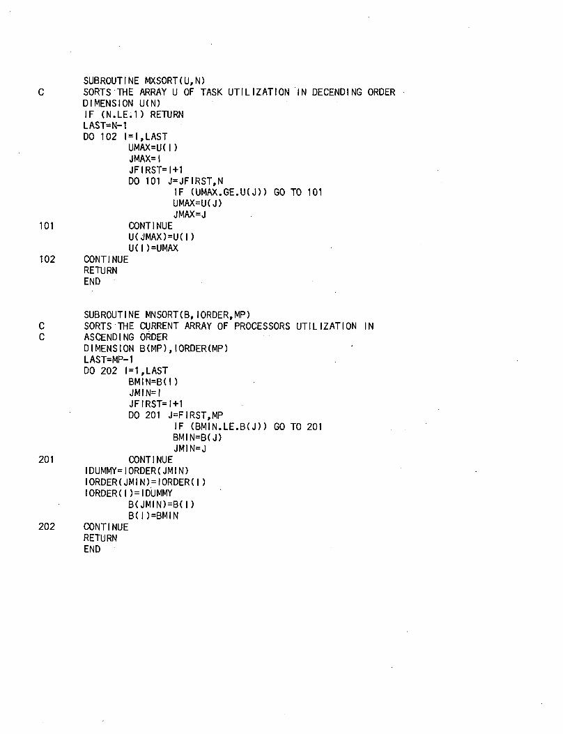
SUBROUTINE MXSORT(U,N)C SORTS THE ARRAY U OF TASK UTILIZATION IN DECENDIN6 ORDER
DIMENSION U(N)IF (N.LE.1) RETURNLAST=N-1DO 102 I=I,LAST
UMAX=U(I)JMAX=IJFIRST=I+1DO 101 J=JFIRST,N
IF (UMAX.GE.UU)> GO TO 101UMAX=U(J)JMAX=J
101 CONTINUEU(JMAX)=U(I)U(I)=UMAX
102 CONTINUERETURNEND
SUBROUTINE MNSORTCB,IORDER,MP)C SORTS THE CURRENT ARRAY OF PROCESSORS UTILIZATION INC ASCENDING ORDER
DIMENSION B(MP),IORDER(MP)LAST=MP-1DO 202 1=1,LAST
BMIN=B(I)JMIN=IJFIRST=I+1DO 201 J=FIRST,MP
IF (BMIN.LE.B(J)) GO TO 201BMIN=B(J)JMIN=J
201 CONTINUEIDUMMY=IORDER(JMIN)IORDER(JMIN)=IORDER(I)IORDER(I)=IDUMMY
B(JMIN)=B(I)B(I)=BMIN
202 CONTINUERETURNEND

Appendix B
The following is a listing
of the modified heuristic algorithmdiscussed in Section 3.1.2.3.

C THIS IS A PROGRAM FOR HEURISTIC APPROACH OF ALLCATING NT TASKSC WITH IR REPLICATIONS TO MP PROCESSORS SO THAT DIFFERENTC REPLICATIONS ARE ALLOCATED TO DISTINCT PROCESSORS ANDC PROCESSOR UTILIZATION IS BALANCEDC PU ARRAY KEEPS TRACK OF UTILIZATION OF PROCESSORSC MU ARRAY KEEPS TRACK OF MEMORY OF PROCESSORSC I ORDER KEEPS THE ORDER OF PROCESSOR UTILIZATION ARRAYC WHEN SORTED IN ASCENDING ORDERC JORDER KEEPS THE ORDER OF TASK UTILIZATION ARRAYC WHEN SORTED IN DESCENDING ORDERC IR=NUMBER OF REPLICATIONS PER TASKC NT=NUMBER OF TASKSC MP=NUMBER OF PROCESSORS
REALM U(40),PM(12)/12*0.0/REAL*4 USUM,UTOTALINTEGER M(40),PM(12)/12*0/INTEGER MSUM,MTOTALINTEGER IORDER(12),JORDER(40),KORDER(5)READ(1,801) IR,NTMAX=NTM=0
10 READ(1,802) X,MXIF (X.EQ.999.) GO TO 20N=N+1JORDER(N)=NIF (N.LE.MAX) U(N)=XIF (N.LE.MAX) M(N)=MXIF (N.LE.MAX) GO TO 10
20 USUM=0.0MSUM=0DO 15 1=1,NT
C ADD THE UTILIZATION AND MEMORY NEEDS OF ALL TASKSUSUM=USUM+U(I)MSUM=MSUM+M(I)
15 CONTINUEC CALCULATE THE NUMBER OF PROCESSORS NEEDEDC UTILIZATION CAPACITY OF A PROCESSOR =0.5C MEMORY CAPACITY OF A PROCESSOR = 20000
USUM=USUM*IRMSUM=MSUM*IRUSUM=USUM/(0.5)MSUM=(MSUM/20000)+1MP=(2*USUM)IF (MP,IT.MSUM) MP=MSUMWRITE(3,901) NT,IR,MPCALL MXSORT(U,N,JORDER)WRITE(3,905)WRITE(3,906)(U(I),J=1,N)
C ASSIGN I REPLICATIONS TO PROCESSORSDO 60 1=1,NT
DO 40 I=1,MPR(I)=PU(I)IORDER(I)=1
40 CONTINUE

CALL MASORKB, IORDER,MP)C II = NUMBER OF REPLICATIONS ASSIGNED SO FAR AT A GIVEN STEPC CHECK = 1 IF MAXIMUM UTILIZATION OR CAPACITY IS ACHIEVEDC KORDER KEEPS TRACK OF ORDER OF PROCESSORS TO WHICHC TASK REPLICATION ARE ASSIGNED AT A GIVEN STEP
11=0DO 50 K=1,MP
UTOTAL=PU(IORDER(K))+U( I)MTOTAL=PM(IORDER(K)+M(JORDER(I))IF ((UTOTAL.GT.(.345)).OR.(MTOTAL.GT.20000)) GO TO 50l l = l l + 1PU(IORDER(K))=UTOTALPM(IORDER(K))=MTOTALKORDER(II)=IORDER(K)IF (II.EQ.IR) GO TO 55
50 CONTINUE55 WRITE(3,903) I
WRITE(3,907) (KORDER(K),K=1,IR)WRITE(3,908)WRITE(3,902) (PU(K),K=1,MP)WRITE(3,909)WRITE(3,910) (PM(K),K=1,MP)
60 CONTINUE801 FORMAT(2I5)802 FORMAT(F7.3,I8)901 FORMAT (//.'NUMBER OF TASKS = !,I4,/,
*' NUMBER OF REPLICATIONS PER TASK = ',I4,/,*' NUMBER OF PROCESSORS = ',I4,//)
902 FORMAT(5X,F6.4)903 FORMAT(/,'REPLICATIONS OF TASK',13,' ARE ASSIGNED TO PROCESSORS')905 FORMATC SORTED DATA')906 FORMAT(4X,F7.3)907 FORMAT(4X,14)908 FORMAT(//,'TOTAL UTILIZATION OF PROCESSORS = ')909 FORMAT(//,'TOTAL MEMORY OF PROCESSORS = ')910 FORMAT(5X,16)
STOPEND
SUBROUTINE MXSORT(U,N,JORDER)C SORTS THE ARRAY U OF TASK UTILIZATION IN DECENDING ORDER
DIMENSION U(N),JORDER(N)IF (N.LE.1) RETURNLAST=N-1DO 102 1=1,LAST
UMAX=U(I)JMAX=IJFIRST=MDO 101 J=JFIRST,N
IF (UMAX.GE.U(J)) GO TO 101UMAX=U(J)JMAX=J
101 CONTINUE

JDUMMY=JORDER(JMAX)JORDER(JMAX)=JORDER(I)JORDER(I)=JDUMMY
U(JMAX)=U(I)U(I)=UMAX
102 CONTINUERETURNEND
SUBROUTINE MNSORT(B,IORDER,MP)C SORTS THE CURRENT ARRAY OF PROCESSORS UTILIZATION INC ASCENDING ORDER
DIMENSION B(MP),IORDER(MP)LAST=MPDO 202 I = 1,LAST
BM1N=B(J)JMIN=IJFIRST=MDO 201 J=JFIRST,MP
IF (BMIN.LE.B(J)) GO TO 201BMIN=B(J)JMIN=J
201 CONTINUEIDUMMY=IORDER(JMIN)IORDER(JMIN)=IORDER(I)IORDER(I)=IDUMMY
B(JMIN)=B(I)B(I)=BMIN
202 CONTINUERETURNEND
Appendix C
This appendix includes computer printoutsof the algorithms discussed inSections 3.1.2.2 and 3.1.2.3.

RUN #1

NUMBER OF TASKS = 23NUMBER OF REPLICATIONS PER TASK = 3NUNBER OF PROCESSORS = 4
SORTED DATA0.1190.0770.0690.0550.0340.0320.0280.0230.0210.0190.0140.0140.0090.0060.0040.0040.0020.0010.0010.0010.0010.0010.001
REPLICATIONS OF TASK 1 ARE ASSIGNED TO PROCESSORS123
TOTAL UTILIZATION OF PROCESSORS =0.11900.11900.11900.0
REPLICATIONS OF TASK 2 ARE ASSIGNED TO PROCESSORS423
TOTAL UTILIZATION OF PROCESSORS =0.11900.19600.19600.0770
REPLICATIONS OF TASK 3 ARE ASSIGNED TO PROCESSORS41

TOTAL UTILIZATION OF PROCESSORS =0.18800.19600.26500.1460
REPLICATIONS OF TASK 4 ARE ASSIGNED TO PROCESSORS412
TOTAL UTILIZATION OF PROCESSORS =0.24300.25100.26500.2010
REPLICATIONS OF TASK 5 ARE ASSIGNED TO PROCESSORS412
TOTAL UTILIZATION OF PROCESSORS =0.27700.28500.26500.2350
REPLICATIONS OF TASK 6 ARE ASSIGNED TO PROCESSORS431
TOTAL UTILIZATION OF PROCESSORS =0.30900.28500.29700.2670
REPLICATIONS OF TASK 7 ARE ASSIGNED TO PROCESSORS423
TOTAL UTILIZATIONS OF PROCESSORS =0.30900.31300.32500.2950
REPLICATIONS OF TASK 8 ARE ASSIGNED TO PROCESSORS4

12
TOTAL UTILIZATIONS OF PROCESSORS =. 0.3320
0.33600,32500.3180
REPLICATIONS OF TASK 9 ARE ASSIGNED TO PROCESSORS431
TOTAL UTILIZATION OF PROCESSORS =0.35300.33600.34600.3390
REPLICATIONS OF TASK 10 ARE ASSIGNED TO PROCESSORS243
TOTAL UTILIZATION OF PROCESSORS =0.35300.35500,36500.3580
REPLICATIONS OF TASK 11 ARE ASSIGNED TO PROCESSORS124
TOTAL UTILIZATION OF PROCESSRS =0.36700.36900,36500.3720
REPLICATIONS OF TASK 12 ARE ASSIGNED TO PROCESSORS312
TOTAL UTILIZATION OF PROCESSORS =0.38100.38300.37900,3720
REPLICATIONS OF TASK 13 ARE ASSIGNED TO PROCESSORS

431
TOTAL UTILIZATION OF PROCESSORS =0.39000.38300.30800.3810
REPLICATIONS OF TASK 14 ARE ASSIGNED TO PROCESSORS423
TOTAL UTILIZATION OF PROCESSORS =0.39000.38900.39400.3870
REPLICATIONS OF TASK 15 ARE ASSIGNED TO PROCESSORS-421
TOTAL UTILIZATION OF PROCESSORS =0.39400.39300.39400.3910
REPLICATIONS OF TASK 16 ARE ASSIGNED TO PROCESSORS421
TOTAL UTILIZATION OF PROCESSORS =0.39800.39700.39400.3950
REPLICATIONS OF TASK 17 ARE ASSIGNED TO PROCESSORS3 . . . . . .42
TOTAL UTILIZATION OF PROCESSORS =0.39800.39900.39600.3970
REPLICATIONS OF TASK 18 ARE ASSIGNED TO PROCESSORS
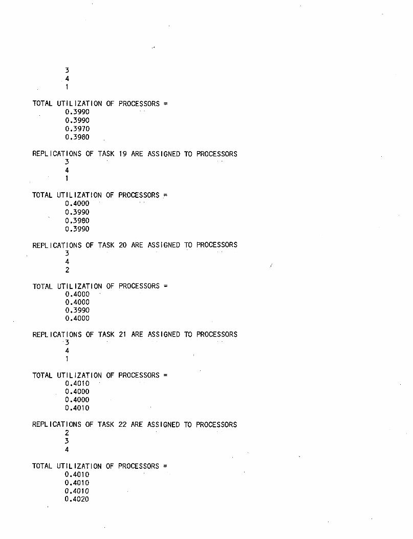
341
TOTAL UTILIZATION OF PROCESSORS =0.39900.39900.39700.3980
REPLICATIONS OF TASK 19 ARE ASSIGNED TO PROCESSORS341
TOTAL UTILIZATION OF PROCESSORS =0.40000.39900.39800.3990
REPLICATIONS OF TASK 20 ARE ASSIGNED TO PROCESSORS3 ' '42
TOTAL UTILIZATION OF PROCESSORS =0.40000.40000.39900.4000
REPLICATIONS OF TASK 21 ARE ASSIGNED TO PROCESSORS341
TOTAL UTILIZATION OF PROCESSORS =0.40100.40000.40000.4010
REPLICATIONS OF TASK 22 ARE ASSIGNED TO PROCESSORS234
TOTAL UTILIZATION OF PROCESSORS =0.40100.40100.40100.4020
REPLICATIONS OF TASK 23 ARE ASSIGNED TO PROCESSORS123
TOTAL UTILIZATION OF PROCESSORS =0.40200.40200.40200.4020

RUN #2

NUMBER OF TASKS = 23NUMBER OF REPLICATIONS PER TASK = 3NUMBER OF PROCESSORS = 5
SORTED DATA0.119
. 0.0770.0690.0550.0340.0320.0280.0230.0210.0190.0140.0140.0090.0060.0040.0040.0020.0010.0010.0010.0010.0010.001
REPLICATIONS OF TASK 1 ARE ASSIGNED TO PROCESSORS123
TOTAL UTILIZATION OF PROCESSORS =0.11900.11900.11900.00.0
REPLICATIONS OF TASK 2 ARE ASSIGNED TO PROCESSORS453
TOTAL UTILIZATION OF PROCESSORS =0.11900.11900.19600.07700.0770
REPLICATIONS OF TASK 3 ARE ASSIGNED TO PROCESSORS

451
TOTAL UTILIZATION OF PROCESSORS =0.18800.11900.19600.14600.1460
REPLICATIONS OF TASK 4 ARE ASSIGNED TO PROCESSORS245
TOTAL UTILIZATION OF PROCESSORS =0.18800.17400.19600.20100.2010
REPLICATIONS OF TASK 5 ARE ASSIGNED TO PROCESSORS213
TOTAL UTILIZATION OF PROCESSORS =0.22200.20800.23000.20100.2010
REPLICATIONS OF TASK 6 ARE ASSIGNED TO PROCESSORS452
TOTAL UTILIZATION OF PROCESSORS =0.22200.24000.23000.23300.2330
REPLICATIONS OF TASK 7 ARE ASSIGNED TO PROCESSORS134
TOTAL UTILIZATION OF PROCESSORS =0.2500

0.24000.25800.26100.2330
REPLICATIONS OF TASK 8 ARE ASSIGNED TO PROCESSORS521
TOTAL UTILIZATION OF PROCESSORS =0.27300.26300.25800.26100.2560
REPLICATIONS OF TASK 9 ARE ASSIGNED TO PROCESSORS534
TOTAL UTILIZATION OF PROCESSORS =0.27300.26300.27900.28200.2770
REPLICATIONS OF TASK 10 ARE ASSIGNED TO PROCESSORS215
TOTAL UTILIZATION OF PROCESSORS =0.29200.28200.27900.28200.2960
REPLICATIONS OF TASK 11 ARE ASSIGNED TO PROCESSORS324
TOTAL UTILIZATION OF PROCESSORS =0.29200.29600.29300.29600.2960
REPLICATIONS OF TASK 12 ARE ASSIGNED TO PROCESSORS

132
TOTAL UTILIZATION OF PROCESSORS =0.30600.31000.30700.29600.2960
REPLICATIONS OF TASK 13 ARE ASSIGNED TO PROCESSORS541
TOTAL UTILIZATION OF PROCESSORS =0.31500.31000.30700.30500.3050
REPLICATIONS OF TASK 14 ARE ASSIGNED TO PROCESSORS543
TOTAL UTILIZATION OF PROCESSORS =0.31500.31000.31300.31100.3110
REPLICATIONS OF TASK 15 ARE ASSIGNED TO PROCESSORS254
TOTAL UTILIZATION OF PROCESSORS =0.31500.31400.31300.31500.3150
REPLICATIONS OF TASK 16 ARE ASSIGNED TO PROCESSORS325
TOTAL UTILIZATION OF PROCESSORS =0.3150
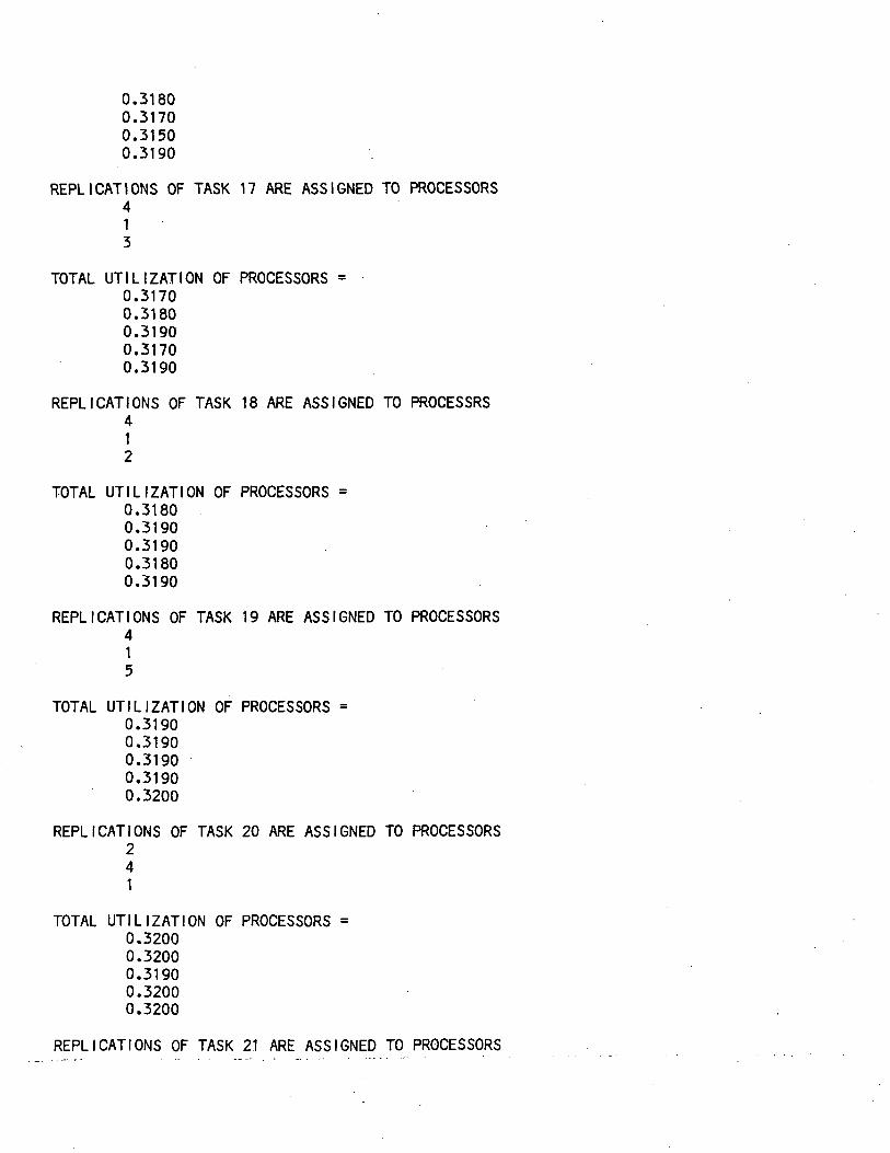
0.31800.31700.31500.3190
REPLICATIONS OF TASK 17 ARE ASSIGNED TO PROCESSORS413
TOTAL UTILIZATION OF PROCESSORS =0.31700.31800.31900.31700.3190
REPLICATIONS OF TASK 18 ARE ASSIGNED TO PROCESSRS412
TOTAL UTILIZATION OF PROCESSORS =0.31800.31900.31900.31800.3190
REPLICATIONS OF TASK 19 ARE ASSIGNED TO PROCESSORS415
TOTAL UTILIZATION OF PROCESSORS =0.31900.31900.31900.31900.3200
REPLICATIONS OF TASK 20 ARE ASSIGNED TO PROCESSORS241
TOTAL UTILIZATION OF PROCESSORS =0.32000.32000.31900.32000.3200
REPLICATIONS OF TASK 2.1 ARE ASSIGNED TO PROCESSORS
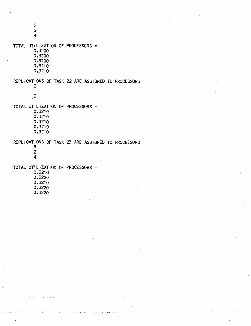
354
TOTAL UTILIZATION OF PROCESSORS =0.32000.32000.32000.32100.3210
REPLICATIONS OF TASK 22 ARE ASSIGNED TO PROCESSORS21,3
TOTAL UTILIZATION OF PROCESSORS =0.32100.32100.32100.32100.3210
REPLICATIONS OF TASK 23 ARE ASSIGNED TO PROCESSORS524
TOTAL UTILIZATION OF PROCESSORS =0.32100.32200.32100.32200.3220

RUN #3
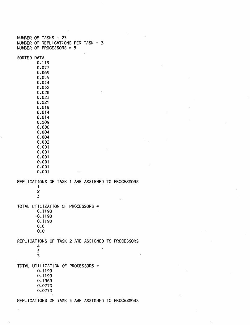
NUMBER OF TASKS = 23NUMBER OF REPLICATIONS PER TASK = 3NUMBER OF PROCESSORS = 5
SORTED DATA0.1190.0770.0690.0550.0340.0320.0280.0230.0210.0190.0140.0140.0090.0060.0040.0040.0020.0010.0010.0010.0010.0010.001
REPLICATIONS OF TASK 1 ARE ASSIGNED TO PROCESSORS123
TOTAL UTILIZATION OF PROCESSORS =0.11900.11900.11900.00.0
REPLICATIONS OF TASK 2 ARE ASSIGNED TO PROCESSORS453
TOTAL UTILIZATION OF PROCESSORS =0.11900.11900.19600.07700.0770
REPLICATIONS OF TASK 3 ARE ASSIGNED TO PROCESSORS

451
TOTAL UTILIZATION OF PROCESSORS =0.18800.11900.19600.14600.1460
REPLICATIONS OF TASK 4 ARE ASSIGNED TO PROCESSORS245
TOTAL UTILIZATION OF PROCESSORS =0.18800.17400.19600.20100.2010
REPLICATIONS OF TASK 5 ARE ASSIGNED TO PROCESSORS213
TOTAL UTILIZATION OF PROCESSORS =0.22200.20800.23000.20100.2010
REPLICATIONS OF TASK 6 ARE ASSIGNED TO PROCESSORS452
TOTAL UTILIZATION OF PROCESSORS =0.22200.2400 .0.23000.23300.2330
REPLICATIONS OF TASK 7 ARE ASSIGNED TO PROCESSORS134
TOTAL UTILIZATION OF PROCESSORS =0.2500

0.24000.25800.26100.2330
REPLICATIONS OF TASK 8 ARE ASSIGNED TO PROCESSORS521
TOTAL UTILIZATION OF PROCESSORS =0.27300.26300.25800.26100.2560
REPLICATIONS OF TASK 9 ARE ASSIGNED TO PROCESSORS534
TOTAL UTILIZATION OF PROCESSORS =0.27300.26300.27900.28200.2770
REPLICATIONS OF TASK 10 ARE ASSIGNED TO PROCESSORS215
TOTAL UTILIZATION OF PROCESSORS =0.29200.28200.27900.28200.2960
REPLICATIONS OF TASK 11 ARE ASSIGNED TO PROCESSORS324
TOTAL UTILIZATION OF PROCESSORS =0.29200.29600.29300.29600.2960
REPLICATIONS OF TASK 12 ARE ASSIGNED TO PROCESSORS

132
TOTAL UTILIZATION OF PROCESSORS =0.30600.31000.30700.29600.2960
REPLICATIONS OF TASK 13 ARE ASSIGNED TO PROCESSORS541
TOTAL UTILIZATION OF PROCESSORS =0.31500.31000.30700.30500.3050
REPLICATIONS OF TASK 14 ARE ASSIGNED TO PROCESSORS543
TOTAL UTILIZATION OF PROCESSORS =0.31500.31000.31300.31100.3110
REPLICATIONS OF TASK 15 ARE ASSIGNED TO PROCESSORS254
TOTAL UTILIZATION OF PROCESSORS =0.31500.31400.31300.31500.3150
REPLICATIONS OF TASK 16 ARE ASSIGNED TO PROCESSORS325
TOTAL UTILIZATION OF PROCESSORS =0.3150

0.31800.31700.31500.3190
REPLICATIONS OF TASK 17 ARE ASSIGNED TO PROCESSORS413
TOTAL UTILIZATION OF PROCESSORS =0.31700.31800.31900.31700.3190
REPLICATIONS OF TASK 18 ARE ASSIGNED TO PROCESSRS412
TOTAL UTILIZATION OF PROCESSORS =0.31800.31900.31900.31800.3190
REPLICATIONS OF TASK 19 ARE ASSIGNED TO PROCESSORS415
TOTAL UTILIZATION OF PROCESSORS =0.31900.31900.31900.31900.3200
REPLICATIONS OF TASK 20 ARE ASSIGNED TO PROCESSORS241
TOTAL UTILIZATION OF PROCESSORS =0.32000.32000.31900.32000.3200
REPLICATIONS OF TASK 21 ARE ASSIGNED TO PROCESSORS
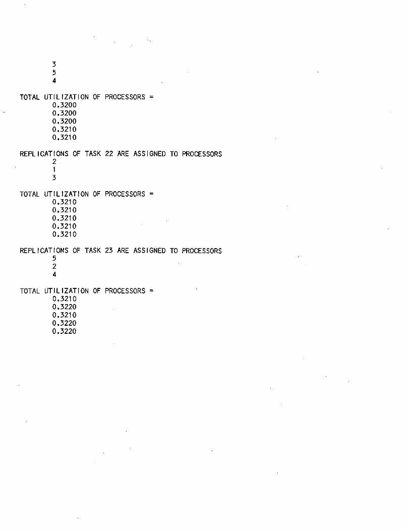
354
TOTAL UTILIZATION OF PROCESSORS =0.32000.32000.32000.32100.3210
REPLICATIONS OF TASK 22 ARE ASSIGNED TO PROCESSORS213
TOTAL UTILIZATION OF PROCESSORS =0.32100.32100.32100.32100.3210
REPLICATIONS OF TASK 23 ARE ASSIGNED TO PROCESSORS524
TOTAL UTILIZATION OF PROCESSORS =0.32100.32200.32100.32200.3220

RUN #4

NUMBER OF TASKS = 23NUMBER OF REPLICATIONS PER TASK = 3NUMBER OF PROCESSORS = 5
SORTED DATA0.1190.0770.0690.0590.0340.0320.0280.0230.0210.0190.0140.0140.0090.0060.0040.0040.0020.0010.0010.0010.0010.0010.001
REPLICATIONS OF TASK 1 ARE ASSIGNED TO PROCESSORS123
TOTAL UTILIZATION OF PROCESSORS =0.11900.11900.11900.00.0
TOTAL MEMORY OF PROCESSORS =150015001500
00
REPLICATIONS OF TASK 2 ARE ASSIGNED TO PROCESSORS453
TOTAL UTILIZATION OF PROCESSORS =

0.11900.11900.19600.07700.0770
TOTAL MEMORY OF PROCESSORS =15001500281013101310
REPLICATIONS OF TASK 3 ARE ASSIGNED TO PROCESSORS451
TOTAL UTILIZATION OF PROCESSRS =0.18000.11900.19600.14600.1460
TOTAL MEMORY OF PROCESSRS =15921500281014021402
REPLICATIONS OF TASK 4 ARE ASSIGNED TO PROCESSORS245
TOTAL UTILIZATION OF PROCESSORS =0.18800.17400.19600.20100.2010
TOTAL MEMORY OF PROCESSORS =
15922525281024272427
REPLICATIONS OF TASK 5 ARE ASSIGNED TO PROCESSORS2

13
TOTAL UTILIZATION OF PROCESSORS =0.22200.20800.28000.20100.2010
TOTAL MEMORY OF PROCESSORS =38424779506024272427
REPLICATIONS OF TASK 6 ARE ASSIGNED TO PROCESSORS452
TOTAL UTILIZATION OF PROCESSORS =0.22200.24000.23000.23300.2330
TOTAL MEMORY OF PROCESSORS =384211025506086778677
REPLICATIONS OF TASK 7 ARE ASSIGNED TO PROCESSORS134
TOTAL UTILIZATION OF PROCESSORS =0.25000.24000.25800.26100.2330
TOTAL MEMORY OF PROCESSORS =439211025561692278677

REPLICATIONS OF TASK 8 ARE ASSIGNED TO PROCESSORS521
TOTAL UTILIZATION OF PROCESSORS =0.27300.26300.25800.26100.2560
TOTAL MEMORY OF PROCESSORS =6467131005610922710752
REPLICATIONS OF TASK 9 ARE ASSIGNED TO PROCESSORS534
TOTAL UTILIZATION OF PROCESSORS =0.27300.26300.27900.28200.2770
TOTAL MEMORY OF PROCESSORS =64671310068101042711952
REPLICATIONS OF TASK 10 ARE ASSIGNED TO PROCESSORS215
TOTAL UTILIZATION OF PROCESSORS =0.29200.28200.27900.28200.2960
TOTAL MEMORY OF PROCESSORS =15807224406810

1042721292
REPLICATIONS OF TASK 11 ARE ASSIGNED TO PROCESSORS324
TOTAL UTILIZATION OF PROCESSORS =0.29200.29600.29300.29600.2960
TOTAL MEMORY OF PROCESSORS =158072250068761048721292
REPLICATIONS OF TASK 12 ARE ASSIGNED TO PROCESSORS132
TOTAL UTILIZATION OF PROCESSORS =0.30600.31000.30700.29600.2960
TOTAL MEMORY OF PROCESSORS =177072440087701048721292
REPLICATIONS OF TASK 13 ARE ASSIGNED TO PROCESSORS541
TOTAL UTILIZATION OF PROCESSORS =0.31500.31000.30760.30500.3050
TOTAL MEMORY OF PROCESSORS =

181372440087701091721722
REPLICATIONS OF TASK 14 ARE ASSIGNED TO PROCESSORS543
TOTAL UTILIZATION OF PROCESSORS =0.31500.31000.31300.31100.3110
TOTAL MEMORY OF PROCESSORS =181372440093881152722332
REPLICATIONS OF TASK 15 ARE ASSIGNED TO PROCESSORS254
TOTAL UTILIZATION OF PROCESSORS =0.31500.31400.31300.31500.3150
TOTAL MEMORY OF PROCESSORS =181372490593801203222837
REPLICATIONS OF TASK 16 ARE ASSIGNED TO PROCESSORS325
TOTAL UTILIZATION OF PROCESSORS =0.31500.31800.31700.3150

0.3190
TOTAL MEMORY OF PROCESSORS =181372520596801203223137
REPLICATIONS OF TASK 17 ARE ASSIGNED TO PROCESSORS413
TOTAL UTILIZATION OF PROCESSORS =0.31700.31800.31900.31700.3190
TOTAL MEMORY OF PROCESSORS =1943725205109801333223137
REPLICATIONS OF TASK 18 ARE ASSIGNED TO PROCESSORS412
TOTAL UTILIZATION OF PROCESSORS =0.31800.31900.31900.31900.31800.3190
TOTAL MEMORY OF PROCESSORS =1999925767109801389423137
REPLICATIONS OF TASK 19 ARE ASSIGNED TO PROCESSORS415
TOTAL UTILIZATION OF PROCESSORS =
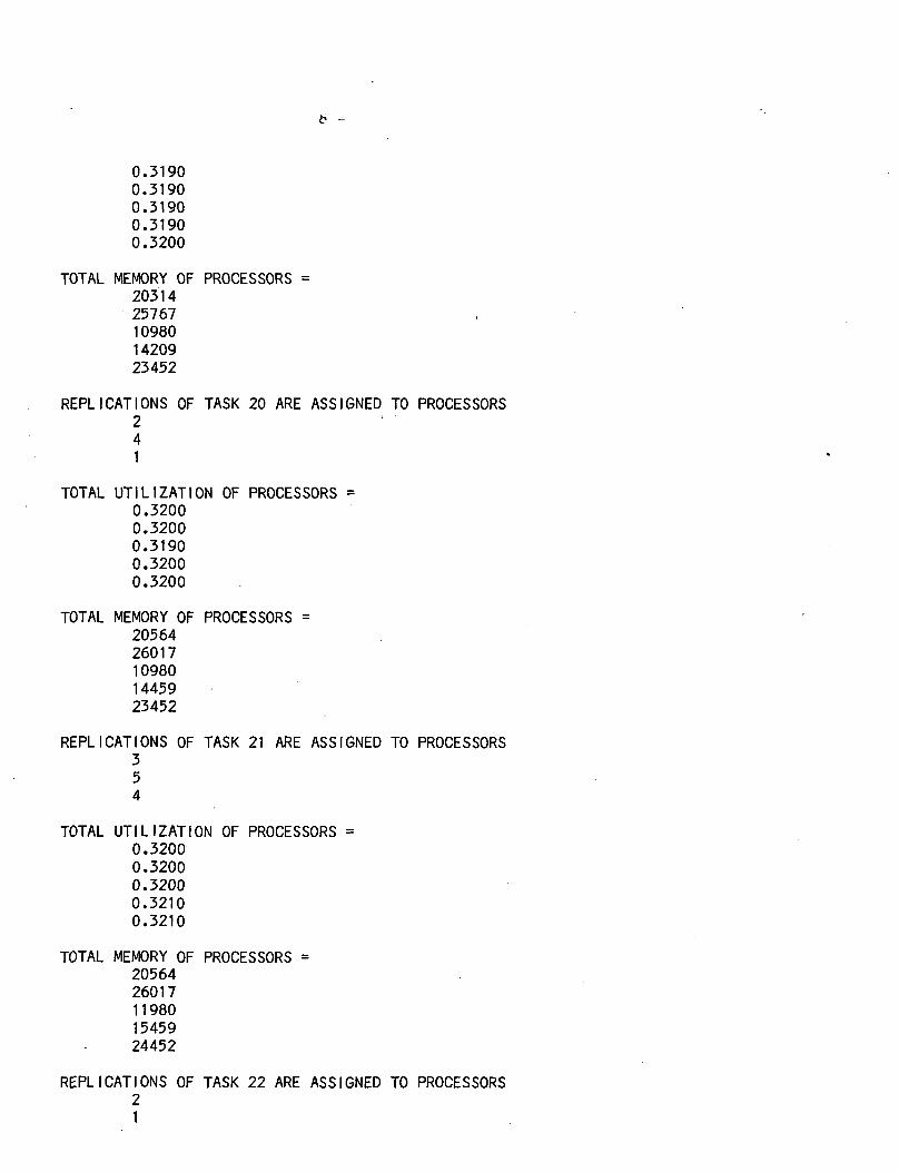
0.31900.31900.31900.31900.3200
TOTAL MEMORY OF PROCESSORS =2031425767109801420923452
REPLICATIONS OF TASK 20 ARE ASSIGNED TO PROCESSORS241
TOTAL UTILIZATION OF PROCESSORS =0.32000.32000.31900.32000.3200
TOTAL MEMORY OF PROCESSORS =2056426017109801445923452
REPLICATIONS OF TASK 21 ARE ASSIGNED TO PROCESSORS354
TOTAL UTILIZATION OF PROCESSORS =0.32000.32000.32000.32100.3210
TOTAL MEMORY OF PROCESSORS =2056426017119801545924452
REPLICATIONS OF TASK 22 ARE ASSIGNED TO PROCESSORS21

TOTAL UTILIZATION OF PROCESSORS =0.32100.32100.32100.32100.3210
TOTAL MEMORY OF PROCESSORS =2156427017129801545924452
REPLICATIONS OF TASK 23 ARE ASSIGNED TO PROCESSORS524
OF PROCESSORS =TOTAL UTILIZATION0.32100.32200.32100.32200.3220
TOTAL MEMORY OF PROCESSORS =2156427152129801559424587

RUN #5

NUMBER OF TASKS = 23NUMBER OF REPLICATIONS PER TASK = 3NUMBER OF PROCESSORS = 6
SORTED DATA0.1190.0770.0690.0550.0340.0320.0280.0230.0210.0190.0140.0140.0090.0060.0040.0040.0020.0010.0010.0010.0010.0010.001
REPLICATIONS OF TASK 1 ARE ASSIGNED TO PROCESSORS123
TOTAL UTILIZATION OF PROCESSORS =0.11900.11900.11900.00.00.0
TOTAL MEMORY OF PROCESSORS =150015001500
000
REPLICATIONS OF TASK 2 ARE ASSIGNED TO PROCESSORS456

TOTAL UTILIZATION OF PROCESSORS =0.11900.11900.11900.07700.07700.0770
TOTAL MEMORY OF PROCESSORS =150015001500131013101310
REPLICATIONS OF TASK 3 ARE ASSIGNED TO PROCESSORS456
TOTAL UTILIZATION OF PROCESSORS =0.11900.11900.11900.14600.14600.1460
TOTAL MEMORY OF PROCESSRS =150015001500140214021402
REPLICATIONS OF TASK 4 ARE ASSIGNED TO PROCESSORS123
TOTAL UTILIZATION OF PROCESSORS =0.17400.17400.17400.14600.14600.1460
TOTAL MEMORY OF PROCESSORS =252525252525
140214021402
REPLICATIONS OF TASK 5 ARE ASSIGNED TO PROCESSRS456
TOTAL UTILIZATION OF PROCESSORS =0.17400.17400.17400.18000.18000.1800
TOTAL MEMORY OF PROCESSORS =2525 <25252525365236523652
REPLICATIONS OF TASK 6 ARE ASSIGNED TO PROCESSORS123
TOTAL UTILIZATION OF PROCESSORS =0.20600.20600.20600.18000.18000.1800
TOTAL MEMORY OF PROCESSORS =877587758775365236523652
REPLICATIONS OF TASK 7 ARE ASSIGNED TO PROCESSORS456
TOTAL UTILIZATION OF PROCESSORS =0.20600.2060

0.20600.20800.20800.2080
TOTAL MEMORY OF PROCESSORS =877587758775420242024202
REPLICATIONS OF TASK 8 ARE ASSIGNED TO PROCESSORS123
TOTAL UTILIZATION OF PROCESSORS =0.22900.22900.22900.20800.20800.2080
TOTAL MEMORY OF PROCESSORS =108501085010850420242024202
REPLICATIONS OF TASK 9 ARE ASSIGNED TO PROCESSORS456
TOTAL UTILIZATION OF PROCESSORS =0.22900.22900.22900.22900.22900.2290
TOTAL MEMORY OF PROCESSORS =108501085010850540254025402

REPLICATIONS OF TASK 10 ARE ASSIGNED TO PROCESSORS123
TOTAL UTILIZATION OF PROCESSORS =0.24800.24800.24800.22900.22900.2290
TOTAL MEMORY OF PROCESSORS =201902019020190540254025402
REPLICATIONS OF TASK 11 ARE ASSIGNED TO PROCESSORS456
TOTAL UTILIZATION OF PROCESSORS =0.24800.24800.24800.24300.24300.2430
TOTAL MEMORY OF PROCESSORS =201902019020190546254625462
REPLICATIONS OF TASK 12 ARE ASSIGNED TO PROCESSORS456
TOTAL UTILIZATION OF PROCESSORS =0.24800.24800.24800.25700.25700.2570
TOTAL MEMORY OF PROCESSORS =201902019020190736273627362
REPLICATIONS OF TASK 13 ARE ASSIGNED TO PROCESSORS123
TOTAL UTILIZATION OF PROCESSORS =0.25700.25700.25700.25700.257.00.2570
TOTAL MEMORY OF PROCESSORS =206202062020620736273627362
REPLICATIONS OF TASK 14 ARE ASSIGNED TO PROCESSORS123
TOTAL UTILIZATION OF PROCESSORS =0.26300.26300.26300.25700.25700.2570
TOTAL MEMORY OF PROCESSORS =212302123021230736273627362
REPLICATIONS OF TASK 15 ARE ASSIGNED TO PROCESSORS456
TOTAL UTILIZATION OF PROCESSORS =0.26300.26300.26300.26100.26100.2610
TOTAL MEMORY OF PROCESSORS =212302123021230786778677867
REPLICATIONS OF TASK 16 ARE ASSIGNED TO PROCESSORS456
TOTAL UTILIZATION OF PROCESSORS =0.26300.26300.26300.26500.26500.265Q
TOTAL MEMORY OF PROCESSORS =212302123021230816781678167
REPLICATIONS OF TASK 17 ARE ASSIGNED TO PROCESSORS123
TOTAL UTILIZATION OF PROCESSORS =0.26500.26500.26500.26500.26500.2650
TOTAL MEMORY OF PROCESSORS =225302253022530

816781678167
REPLICATIONS OF TASK 18 ARE ASSIGNED TO PROCESSORS123
TOTAL UTILIZATION OF PROCESSORS =0.26600.26600.26600.26500.26500.2650
TOTAL MEMORY OF PROCESSORS =230922309223092816781678167
REPLICATIONS OF TASK 19 ARE ASSIGNED TO PROCESSORS4 .56
TOTAL UTILIZATION OF PROCESSORS =0.26600.26600.26600.26600.26600.2660
TOTAL MEMORY OF PROCESSORS =230922309223092848284828482
REPLICATIONS OF TASK 20 ARE ASSIGNED TO PROCESSORS123
TOTAL UTILIZATION OF PROCESSORS =0.26700.2670

0.26700.26600.26600.2660
TOTAL MEMORY OF PROCESSORS =233422334223342848284828482
REPLICATIONS OF TASK 21 ARE ASSIGNED TO PROCESSORS456
TOTAL UTILIZATION OF PROCESSORS =0.26700.26700.26700.26700.26700.2670
TOTAL MEMORY OF PROCESSORS =233422334223342948294829482
REPLICATIONS OF TASK 22 ARE ASSIGNED TO PROCESSORS123
TOTAL UTILIZATION OF PROCESSORS =0.26800.26800.26800.26700.26700.2670
TOTAL MEMORY OF PROCESSORS =243422434224342948294829482
REPLICATIONS OF TASK 23 ARE ASSIGNED TO PROCESSORS456
TOTAL UTILIZATION OF PROCESSORS =0.26800.26800.26800.26800.26800.2680
TOTAL MEMORY OF PROCESSORS =243422434224342961796179617

RUN #6

NUMBER OF TASKS = 23NUMBER OF REPLICATIONS PER TASK = 3NUMBER OF PROCESSORS = 6
SORTED DATA0.1190.0770.0690.0550.0340.0320.0280.0230.0210.0190.0140.0140.0090.0060.0040.0040.0020.0010.0010.0010.0010.0010.001
REPLICATIONS OF TASK 1 ARE ASSIGNED TO PROCESSORS123
TOTAL UTILIZATION OF PROCESSORS =0.11900.11900.11900.00.00.0
TOTAL MEMORY OF PROCESSORS =150015001500
000
REPLICATIONS OF TASK 2 ARE ASSIGNED TO PROCESSORS456

TOTAL UTILIZATION OF PROCESSORS =0.11900.11900.11900.07700.07700.0770
TOTAL MEMORY OF PROCESSORS =150015001500131013101310
REPLICATIONS OF TASK 3 ARE ASSIGNED TO PROCESSORS456
TOTAL UTILIZATION OF PROCESSORS =0.11900.11900.11900.14600.14600.1460
TOTAL MEMORY OF PROCESSORS =150015001500140214021402
REPLICATIONS OF TASK 4 ARE ASSIGNED TO PROCESSORS123
TOTAL UTILIZATION OF PROCESSORS =0.17400.17400.17400.14600.14600.1460
TOTAL MEMORY OF PROCESSORS =252525252525
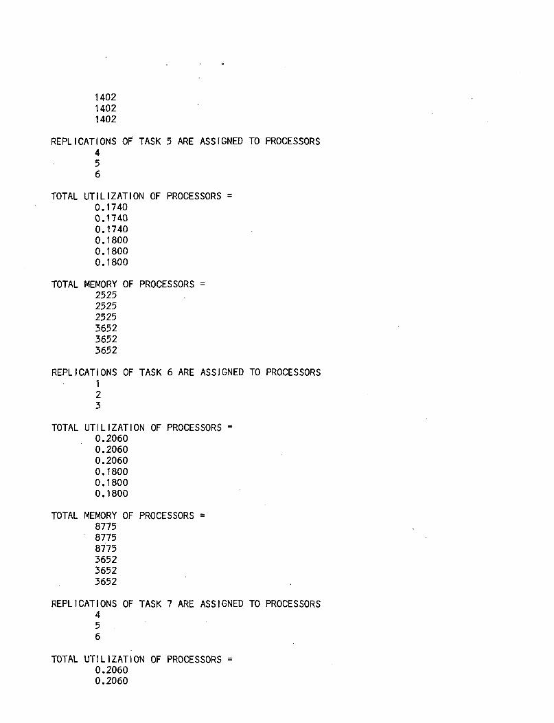
140214021402
REPLICATIONS OF TASK 5 ARE ASSIGNED TO PROCESSORS456
TOTAL UTILIZATION OF PROCESSORS =0.17400.17400.17400.18000.18000.1800
TOTAL MEMORY OF PROCESSORS =252525252525365236523652
REPLICATIONS OF TASK 6 ARE ASSIGNED TO PROCESSORS123
TOTAL UTILIZATION OF PROCESSORS =0.20600.20600.20600.18000.18000.1800
TOTAL MEMORY OF PROCESSORS =877587758775365236523652
REPLICATIONS OF TASK 7 ARE ASSIGNED TO PROCESSORS456
TOTAL UTILIZATION OF PROCESSORS =0.20600.2060

0.20600.20800.20800.2080
TOTAL MEMORY OF PROCESSORS =877587758775420242024202
REPLICATIONS OF TASK 8 ARE ASSIGNED TO PROCESSORS123
TOTAL UTILIZATION OF PROCESSORS =0.22900.22900.22900.20800.20800.2080
TOTAL MEMORY OF PROCESSORS =108501085010850420242024202
REPLICATIONS OF TASK 9 ARE ASSIGNED TO PROCESSORS456
TOTAL UTILIZATION OF PROCESSORS =0.22900.22900.22900.22900.22900.2290
TOTAL MEMORY OF PROCESSORS =108501085010850540254025402

REPLICATIONS OF TASK 10 ARE ASSIGNED TO PROCESSORS456
TOTAL UTILIZATION OF PROCESSORS =0.22900.22900.22900.24800.24800.2480
TOTAL MEMORY OF PROCESSORS =108501085010850147421474214742
REPLICATIONS OF TASK 11 ARE ASSIGNED TO PROCESSORS123
TOTAL UTILIZATION OF PROCESSORS =0.24300.24300.24300.24800.24800.2480
TOTAL MEMORY OF PROCESSORS =109101091010910147421474214742
REPLICATIONS OF TASK 12 ARE ASSIGNED TO PROCESSORS123
TOTAL UTILIZATION OF PROCESSORS =0.25700.25700.25700.24800.24800.2480

TOTAL MEMORY OF PROCESSORS =128101281012810147421474214742
REPLICATIONS OF TASK 13 ARE ASSIGNED TO PROCESSORS456
TOTAL UTILIZATION OF PROCESSORS =0.25700.25700.25700.25700.25700.2570
TOTAL MEMORY OF PROCESSORS =128101281012810151721517215172
REPLICATIONS OF TASK 14 ARE ASSIGNED TO PROCESSORS123
TOTAL UTILIZATION OF PROCESSORS =0.26300.26300.26300.25700.25700.2570
TOTAL MEMORY OF PROCESSORS =134201342013420151721517215172
REPLICATIONS OF TASK 15 ARE ASSIGNED TO .PROCESSORS456
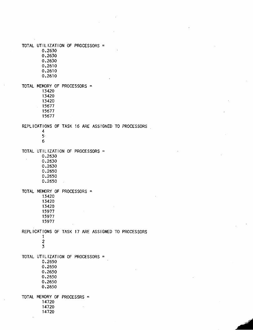
TOTAL UTILIZATION OF PROCESSORS =0.26300.26300.26300.26100.26100.2610
TOTAL MEMORY OF PROCESSORS =134201342013420156771567715677
REPLICATIONS OF TASK 16 ARE ASSIGNED TO PROCESSORS456
TOTAL UTILIZATION OF PROCESSORS =0.26300.26300.26300.26500.26500.2650
TOTAL MEMORY OF PROCESSORS =134201342013420159771597715977
REPLICATIONS OF TASK 17 ARE ASSIGNED TO PROCESSORS123
TOTAL UTILIZATION OF PROCESSORS =0.26500.26500.26500.26500.26500.2650
TOTAL MEMORY OF PROCESSRS =147201472014720
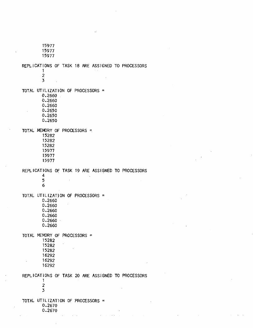
159771597715977
REPLICATIONS OF TASK 18 ARE ASSIGNED TO PROCESSORS123
TOTAL UTILIZATION OF PROCESSORS =0.26600.26600.26600.26500.26500.2650
TOTAL MEMORY OF PROCESSORS =152821528215282159771597715977
REPLICATIONS OF TASK 19 ARE ASSIGNED TO PROCESSORS4 .56
TOTAL UTILIZATION OF PROCESSORS =0.26600.26600.26600.26600.26600.2660
TOTAL MEMORY OF PROCESSORS =152821528215282162921629216292
REPLICATIONS OF TASK 20 ARE ASSIGNED TO PROCESSORS123
TOTAL UTILIZATION OF PROCESSORS =0.26700.2670
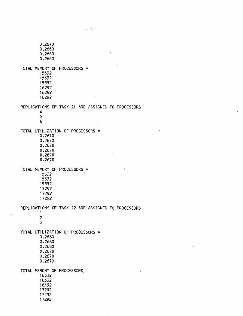
0.26700.26600.26600.2660
TOTAL MEMORY OF PROCESSORS =155321553215532162921629216292
REPLICATIONS OF TASK 21 ARE ASSIGNED TO PROCESSORS456
TOTAL UTILIZATION OF PROCESSORS =0.26700.26700.26700.26700.26700.2670
TOTAL MEMORY OF PROCESSORS =155321553215532172921729217292
REPLICATIONS OF TASK 22 ARE ASSIGNED TO PROCESSORS123
TOTAL UTILIZATION OF PROCESSORS =0.26800.26800.26800.26700.26700.2670
TOTAL MEMORY OF PROCESSORS =165321653216532172921729217292

REPLICATIONS OF TASK 23 ARE ASSIGNED TO PROCESSORS456
TOTAL UTILIZATION OF PROCESSORS =0.26800.26800.26800.26800.26800.2680
TOTAL MEMORY OF PROCESSORS =165321653216532174271742717427

1. Report No. . 2. Government Accession No.
1659264. Title and Subtitle
PROBLEMS RELATED TO THE INTEGRATION OFFAULT-TOLERANT AIRCRAFT ELECTRONIC SYSTEMS
7. Author(s) . . -
J. A. Bannister, K. Trivedi,V. Adlakha, and T. A. Alspaugh, Jr.
9. Performing Organization Name and Address
Systems and Measurements DivisionResearch Triangle InstituteP.O. Box 12194Research Triangle Park, NC 27709
12. Sponsoring Agency Name and Address
National Aeronautics and Space AdministrationWashington * DC 20546
3. Recipient's Catalog No.
5. Report DateJune 1982
6. Performing Organization Code
8. Performing Organization Report No.
505-34-43-0610. Work Unit No.
11. Contract or Grant No.
NAS1-1648913. Type of Report and Period Covered
Contractor Report14. Sponsoring Agency Code
15. Supplementary Notes
16. Abstract
This report explores several problems related to the design of integratedfault-tolerant aircraft electronic systems.
Problems related to the design of the hardware for an integrated aircraft electronicsystem are first considered. Taxonomies of concurrent systems are reviewed and anew taxonomy is proposed. An informal, methodology intended to identify feasibleregions of the taxonomic design space is described. Specific tools are recommendedfor use in the methodology. Based on the methodology, a preliminary "strawman"integrated .fault-tolerant aircraft electronic system is. proposed.
Next, problems related to the programming and control of integrated aircraftelectronic systems are discussed. Issues of system resource management, includingthe scheduling and allocation of real-time periodic tasks in a multiprocessorenvironment, are treated in detail. The role of software design in integratedfault-tolerant aircraft electronic systems is .discussed.
Conclusions and recommendations for.further work are included.
17. Key Words (Suggested by Author(s))
design methodology, fault- toleranceintegrated aircraft electronic systems,multiprocessor taxonomy, .real-timeperiodic scheduling, reliability, softwareengineering, task allocation
19. Security Classif. (of this report)
Unclassified
18. Distribution Statement
Unclassified - Unlimited
Subject Category 61
20. Security Classif. (of this page) 21. No. of Pages 22. Price"
Unclassified 168
N-305 For sale by the National Technical Information Service, Springfield, Virginia 22161