Embed Size (px)
Citation preview

Mathematical Geology, Vol. 22, No. 5, 1990
Problems in Space-Time Kriging of Geohydrological Data 1
Shahrokh Rouhani 2 and Donald E. Myers 3
Spatiotemporal variables constitute a large class of geohydrological phenomena. Estimation of these variables requires the extension of geostatistical tools into the space-time domain. Before applying these techniques to space-time data, a number of important problems must be addressed. These problems can be grouped into four general categories: (1) fundamental differences with respect to spatial problems, (2) data characteristics, (3) structural analysis including valid models, and (4) space-time kriging. Adequate consideration of these problems leads to more appropriate estimation techniques for spatiotemporal data.
KEY WORDS: geostatistics, geohydrology, kriging, spatiotemporal variables.
I N T R O D U C T I O N
There are many geohydrological variables that can be viewed as spatiotemporaI phenomena. For example, piezometric readings or monthly rainfall exhibit ran- dom aspects both with respect to time and to space. The estimation of such variables at unsampled spatial locations or unsampled times requires extending the usual geostatistical techniques into the space-time domain.
Despite the apparent straightforward appearance of such an extension, there are a number of theoretical and practical problems that must be resolved prior to the successful application of geostatistical methods. These problems seem to have received less than an adequate amount of attention. In part this is due to the traditional applications of geostatistics wherein only spatial or only temporal dependence, but not both, need be considered. In some instances the problems are avoided by removing one or the other forms of the dependence in some manner. Let y(x, t) be a variable of interest defined in a region of space and also in a domain of time; for example, y might be the infiltration rate at location
tManuscript received 29 August 1989; accepted 31 October 1989. 2School of Civil Engineering, Georgia Institute of Technology, Atlanta, Georgia 30332. 3Department of Mathematics, University of Arizona, Tucson, Arizona 85721.
611
0882-8121/90/0700-061 I $06.00/1 © 1990 International Association for Mathematical Geology

612 Rouhani and Myers
x and on day (or time) t. New variables can be defined in a number of ways, e.g.,
Zl(X)= fry(x,t)dt or z2(x)=(1/T) fry(x,t)dt (1)
Measuring time in days already suggests that the time dependence has been altered from instantaneous to the cumulative or average value for the day. This could be extended further to monthly or yearly averages, for sufficiently long periods the values might be treated as replications of the same variable in space. For a small number of intermediate-length time periods, the values might be treated as different variables. Examples of some of these approaches can be found in Delhomme (1978), Chua and Bras (1980), and Rouhani (1986) among others. Alternatively, the spatial dependence might be removed by using spatial averages, usually leading to the use of time-series methods.
w,( t ) = fAY(X,t) dx or w2(t) =(1/A) fAY(X,t) dx (2)
None of these approaches is completely satisfactory since there is some loss of information, in particular before using one of these, it should be determined whether the spatial or temporal dependence is dominant. Inadvertent removal of the dominant source of variability could result in a significant loss of infor- mation. If the temporal dependence is removed, then the phenomena is treated as static rather than as dynamic.
It would seem then that the best approach is to treat the variable of interest as is suggested by the notation y(x, t)--that is, time is treated as another di- mension. In general, the dependence of y on x is related to its dependence on t and conversely. There are only a few examples in print of attempts to model functions in this more general form. Bilonick (1985, 1987) used nested vario- grams to model and krige an atmospheric chemical deposition data set. Egbert and Lettenmaier (1986) used a similar approach for similar data. Rouhani and Hall (1989) used intrinsic random functions for space-time kriging of piezo- metric data. However, little attention has been given to the problems associated with treating time simply as another dimension.
FUNDAMENTAL DIFFERENCES
As noted by Joumel (1986, p. 120), there are major differences between spatial and temporal phenomena. In most cases the function or variable of in- terest is unique and the uncertainty or stochastic nature of the problem reflects a lack of knowledge about the values at unsampled locations or the functional

Space-Time Kriging of Geohydrological Data 613
form. While there may be some directional dependence (i.e., an anisotropy), there is in general no ordering, whereas for temporal phenomena there is always the notion of past, present, and future. Although spatial variables of interest are treated as realizations of a random function, i.e.,
= z ( x , , (3 )
where xi denotes a location in space and coj is the element of the underlying probability space or index on the realizations, this stochastic dependence is usually suppressed. [See, e.g., De Marsily and Ahmed (1987, p. 58) with re- spect to the modeling of transmissivity.]
This approach may not be fully satisfactory when time is treated as simply another dimension and the variable is considered a unique realization of a ran- dom function defined in space and time. For example, piezometric head might represent a unique realization for the past and present, but in the case of the future there is a truer stochastic dependence. For some variables this dilemma can be resolved by taking advantage of a periodicity in time, by considering the variable over multiple time periods which might be treated as multiple real- izations. The difficulty lies in determining the temporal extent of each realiza- tion, in particular these may not be of constant length. Because the spatial extent of the region of interest is always taken to be finite and generally is considered fixed, periodicities in space are not often modeled. For example Journel and Froideveaux (1982) concluded in one instance that there was very little im- provement in the estimator by modeling a spatial periodicity with a hole effect variogram. It seems less likely that modeling a temporal periodicity by using a hole-effect variogram would produce an improved estimator. A further compli- cation may occur if the time domain is segmented to generate multiple real- izations; these are often correlated and it becomes necessary to consider the multiple "realizations" as single realizations of several correlated random func- tions. The analysis in this case requires the use of cross-variograms and co- kriging.
The most important difference is not so much that between spatial and temporal problems, but rather that between spatiotemporal problems and either of the two simpler models. In the spatial context or in the temporal context one can construct a valid covariance or variogram easily (i.e., by starting with known valid models such as the spherical, exponential, Gaussian, etc.). Valid vario- grams are obtainable as positive linear combinations. In the case of co- variances, positive linear combinations and products are valid covariances. These constructions are in general not valid if combining a valid temporal model with a valid spatial model to produce a spatiotemporal model. This is essentially the same problem as attempting to construct a valid model in 2-space from models valid in 1-space. This will be discussed in greater detail in the section on Structural Analysis.

614 Rouhani and Myers
TYPICAL DATA CHARACTERISTICS
Normally, geohydrologic data, such as piezometric data, are composed of few scattered clusters of observation wells with long time series at each point. Similar configurations could also be found in precipitation or atmospheric chemical data sets. Such conditions are dictated by the economy of sampling and the accessibility of sampling sites. The main factor seems to be the rela- tively high cost of establishment of an observation station, which usually leads to more intense sampling at the already existing sites.
The above condition creates a situation wherein there is a disparity in the amount of information available in the spatial and temporal domains. This means that the data is usually dense in the temporal domain but sparse in the spatial domain. Such a circumstance often results in estimates of the spatial and tem- poral structures with quite different degrees of reliability and accuracy.
Geohydrological space-time data often exhibits another characteristic, that of periodicity in time and nonstationarity in space. The temporal periodicity is usually reflected in the mean, which can be modeled by a variety of functions, including diurnal and seasonal cycles with relatively stable periods but with varying amplitudes and phases. More specifically, periodic mean functions could be represented as sums of sines and cosines but with coefficients that are random variables. One of the difficulties in using such a representation is that of esti- mating the unknown parameters. Seguret (1989) has proposed a solution in the context of universal kriging.
Climatic Cycles represent a second type of temporal trend in that they are only quasiperiodic: not only will the periods vary but so will the amplitudes and phases. To adequately detect and model such trends, one must observe time series over a very long time. If the data is observed or analyzed by the use of moving windows, whose length is less than the approximate periods of the cycles, then the trend may simply appear as linear or quadratic. In such a case the quasiperiodic trend may not be distinguishable from a true nonperiodic trend. The latter are a third type of trend which may reflect long-term climatic or man- made changes.
In addition to nonstationarities with respect to time, often there are non- periodic spatial nonstationarities governed by geographical and topographical conditions. The modeling of these nonstationarities can give rise to a number of problems. Usually, the nonconstant drift, whether temporal or spatial, is modeled by a linear combination of basic functions. The basic functions are usually taken to be monomials in the position coordinates or sines and cosines ]i.e., the general class of polynomials as noted in Chauvet (1982)]. Omre (1987) has proposed the use of a much wider class of drift functions in the context of a Bayesian prior. In all such problems one is faced with the question of how to estimate/model the drift with first determining the variograms and how to es- timate/model the variogram without first determining the drift. As noted in

Space-Time Kriging of Geohydrological Data 615
Myers (1989), the partitioning of the random function into a random stationary part and a deterministic drift part is not unique, and consequently the variogram may be indeterminate. Obviously one cannot solve the kriging equations with- out knowing the order of the drift and the variogram. One way to resolve this conundrum is to use intrinsic random functions of order k and an automatic structure recognition as described by Delfiner (1976). That algorithm, however, is only directly applicable to drift functions that are monomials. On the other hand, if a moving neighborhood is used in the kriging, it may be possible to consider all components of the drift function as approximated by monomials as suggested by Rouhani and Hall (1989).
The nonstationarity is not always limited to the first moment. In many cases, even when local stationarity of mean can be assumed, strong differences in the variances are observed at different sites. For instance, the portions of an aquifer, which are in a closer hydraulic contact with surface waters, often ex- hibit a wider range of variation, when compared to the more confined zones.
The above conditions may require some modifications due to the usual stationarity requirements of geostatistical procedures. The typical practical rem- edies in the spatial context include removing of the outlier sites in the structural analysis, or dividing the data sets into more homogeneous subsets. The small size of a typical groundwater data set, specially in space, may prohibit such modifications.
STRUCTURAL ANALYSIS
As suggested above, the most reasonable method for extending into the spatiotemporal domain is to treat time as another dimension. There are two ways to utilize this extension to model variograms and covariances: (1) keep the spatial and temporal coordinates completely separate; and (2) introduce a distance into this higher dimensional space and treat geometric anisotropies in a manner analogous in Euclidean space (i.e., use an affine transformation to transform to an isotropic model). Components dependent on time or space co- ordinates only would correspond to zonal anisotropies. One must, of course, verify that the resulting model is valid and that the kriging system has a unique solution.
Perhaps the easiest way to extend from both domains to the spatiotemporat domain is to represent the random function as a simple construct of models in the separate domains. For example, suppose that Y(x, t) = Z ( x ) + U( t ) or Y(x, t) = Z ( x ) U ( t ) , where Z(x) , U(t ) are assumed to be independent or at least uncorrelated. Important special cases include those where one or the other of the two components is deterministic. In the case of the sum, this would correspond to a spatial random function with the drift dependent on time or conversely. In the case of a product, this would correspond to the sill of the

616 Rouhani and Myers
spatial variogram being time-dependent or the sill of the temporal variogram being spatially dependent. Several authors have used models corresponding to these constructions, e.g. ,
C(h, t) = Ct(t)Ch(h ) (4a)
(Rodriguez-Iturbe and Mejia, 1974),
T(h, t) = 3"0 + T,( t ) + 3"h(h) + 3'h,,([gh 2 + ?]0.5) (4b)
(Bilonick, 1987),
GC(h, t) = GCt(t) + GCh(h) (4c)
(Rouhani and Hall, 1989), where,
C = spatiotemporal covariance
C, = temporal covariance
Ce = spatial covariance
3' = spatiotemporal variogram
3'0 = nugget effect
3', = temporal variogram
3'h = spatial variogram
3'h,, = isotropic space-time variogram
GC = spatiotemporal generalized (polynomial) covariance
GC~ = temporal generalized covariance
GCh = spatial generalized covariance
g = geometric coefficient of anisotropy between space and time
h = space lag
t = time lag
An examination of the literature in (spatial) geostatistics suggests that geo- metric anisotropies are modeled occasionally, but it is much more common to use an isotropic model for several reasons: (1) there may be an insufficient number of sample locations in the various directions; (2) even with an adequate number of pairs for most lags, it may be that the directional variograms are more difficult to model than one isotropic variogram; (3) the geometric anisot- ropy only incorporates a change in the range; (4) anisotropies are sometimes indistinguishable from nonconstant drift; and (5) assumed or known properties

Space-Time Kriging of Geohydroiogical Data 617
of the phenomena are external from the variogram computations, which support or suggest isotropy. There are practically no examples in the literature for non- geometric anisotropic variograms. This suggests that such modeling, when ex- tended into the spatiotemporal domain, is much more difficult. The difficulty is exacerbated because the extent of sampling in the time domain is usually quite different from that in the spatial context. Drilling additional wells for making piezometric head readings is expensive, whereas making additional observa- tions over time is relatively inexpensive. Given that variogram modeling in the spatial context is partially subjective, the difficulty is substantially compounded when extended into the spatiotemporal domain. Some of these problems are shown in the following two examples.
Example 1
Several of the space-time variogram or covariance models cited above were constructed under the premise that a positive linear combination of variograms or covariances (and in the case of covariances, a product) is a valid model-- that is, if the components separately satisfy the appropriate positive definiteness condition, then the sum (or product) satisfies the same condition. Joumel and Myers (1989) have shown that this is generally not true when the components are functions of only a part of the components of the position vector. Specifi- cally, it is shown that if a sum of two components is considered, one a function of the horizontal distance only and the other a function of the vertical distance only, that the result is not a valid model in two-dimensional space. The follow- ing is a recasting of that example for the case of a two-dimensional space where one component is time.
Consider four points in (x, t) space (x in one-dimensional space) with coordinates as follows: Point 1:(0, 0), Point 2:(0, ~), Point 3:(c~, 0), Point 4 : (a , z) and a variogram model is constructed to represent a zonal anisotropy as follows:
v(h, t) : vh(h) + V,(t) (5t
Suppose that 7h(O) = O, 3,h(O~) = U, 7,(0) = O, %(~') = V, and consider the coefficient matrix for ordinary kriging when using these four data locations
m
0 u v u + v 1
u 0 u + v v t
v u + v 0 u 1
u + v v u 0 1
1 1 1 1 0
( 6 )

618 Rouhani and Myers
It is easily seen that this matrix is singular and hence the kriging system will not have a Unique solution. The specific cause of the singularity is that the constructed variogram (5) is not strictly conditionally positive-definite but rather only semi-definite. Note that very little was assumed about the variograms that are the subcomponents, and hence the counter-example is very general. In par- ticular the subcomponents might well be models that are valid in arbitrary di- mensions [i.e., the problem does not arise because of the difficulties associated with the counter-example given by Armstrong and Jabin (1981)]. They show that the "truncated" linear model (linear up to a range and then with a sill) is valid in one-dimensional space but not in higher-dimensional space. The zonal anisotropy in (5) is obtained by two transformations; the first maps the point (x, t) (in 2-space) onto the point x (in 1-space), whereas the second one maps the point (x, t) onto the point t. Neither of these transformations is one-to-one (i.e., they are not invertible). While the coefficient matrix will not fail to be invertible for all sample location patterns, it will fail for all patterns that are rectangles with sides parallel to the coordinate axes. One could also construct less obvious examples by rotating the axes.
Example 2
The use of positive linear combinations of valid generalized covariance functions, such as the third model in Eq. (4), causes another problem, concern- ing the family of admissible polynomial covariance functions. For instance, as suggested by Rouhani and Hall (1989), one can conduct separate automatic structural analysis in the two-dimensional space and the one-dimensional time, such that orders of the drifts can be determined. In the case of second-order space and time drifts, the monomials will include 1, x, y, x 2, y 2 t, and t 2. One can further estimate the parameters of the two generalized covariances, such that they be admissible in space and time, respectively. This approach, how- ever, is not equivalent to a three-dimensional process with second-order drift, because it ignores the composite space-time monomials, such as xt and yt. In other words, the three-dimensional intrinsic random function approach, as sug- gested by Matheron (1973), is modified by including only selected monomials in our estimation process. Consequently, the functional form of the admissible family of generalized covariance functions should be modified, too. This mod- ified form of the generalized covariances is rather complex and has not been determined yet (Matheron, 1979, p. 29). So, the linear combinations of two- dimensional space generalized covariances and one-dimensional temporal gen- eralized covariances may not constitute all the admissible functions. Alterna- tives for avoiding the difficulties listed above are discussed in the next section in the context of co-kriging.
Space-Time Kriging of Geohydrological Data 619
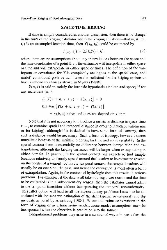
S P A C E - T I M E K R I G I N G
If time is simply considered as another dimension, then there is no change in the form of the kriging estimator nor in the kriging equations--that is, if (x0, to) is an unsampled location-time, then Y(xo, to) could be estimated by
Y(xo, to) = Z XiY(xi, ti) (7)
where there are no assumptions about any interrelations between the space and the time coordinates of a point (i.e., the estimator will interpolate in either space or time and will extrapolate in either space or time). The definition of the var- iogram or covariance for Y is completely analogous to the spatial case, and (strict) conditional positive definiteness is sufficient for the kriging system to have a unique solution as shown in Myers (1988b).
Y(x, t) is said to satisfy the intrinsic hypothesis (in time and space) if for any increment (h, t)
E [ Y ( x + h, + t) - r ( x , 7) ] : o
0.5 Var [Y(x + h, r + t) - Y(x, ~-)]
= "y(h, t) exists and does not depend on x or 7-
Note that it is not necessary to introduce a metric or distance in space-time (i.e., to combine spatial and temporal distance in order to introduce variograms or for kriging), although if it is desired to have some form of isotropy, then such a distance would be necessary. Such a form of isotropy, however, seems unrealistic because of the intrinsic ordering for time and nonreversibility. In the spatial context there is essentially no difference between interpolation and ex- trapolation, although the kriging variances will be larger when extrapolating in either domain. In general, in the spatial context one expects to find sample locations relatively uniformly spread around the location to be estimated (except on the border of a region), but in the temporal context the sample locations will usually be on one side, the past, and hence the estimation is most often a form of extrapolation. Again, in the context of hydrologic data this results in serious problems. For example, if the data is all taken during a wet season and the time to be estimated is in a subsequent dry season, then the estimator cannot adapt to the temporal transition without incorporating the temporal nonstationarity. This latter option will lead to all the indeterminacy problems known to be as- sociated with the separate estimation of the drift (spatial or temporal) and the residuals as noted by Armstrong (1984). Where the estimator is written in the form of kriging or as a time series model, some model assumptions must be incorporated when the objective is prediction into the future.
Computational problems may arise in a number of ways: in particular, the
620 Rouhani and Myers
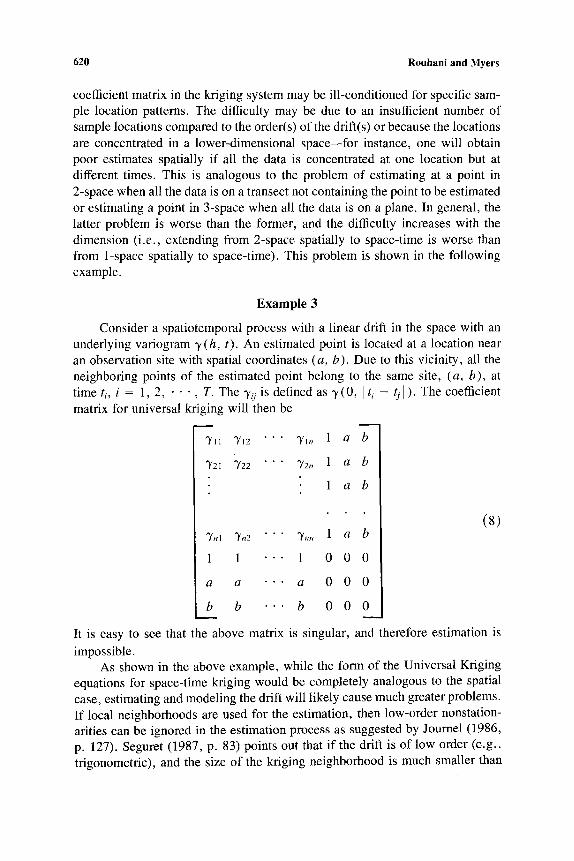
coefficient matrix in the kriging system may be ill-conditioned for specific sam- ple location patterns. The difficulty may be due to an insufficient number of sample locations compared to the order(s) of the drift(s) or because the locations are concentrated in a lower-dimensional space--for instance, one will obtain poor estimates spatially if all the data is concentrated at one location but at different times. This is analogous to the problem of estimating at a point in 2-space when all the data is on a transect not containing the point to be estimated or estimating a point in 3-space when all the data is on a plane. In general, the latter problem is worse than the former, and the difficulty increases with the dimension (i.e., extending from 2-space spatially to space-time is worse than from 1-space spatially to space-time). This problem is shown in the following example.
Example 3
Consider a spatiotemporal process with a linear drift in the space with an underlying variogram 3, (h, t). An estimated point is located at a location near an observation site with spatial coordinates (a, b). Due to this vicinity, all the neighboring points of the estimated point belong to the same site, (a, b), at time t i , i = 1, 2 , • • " , T . The ~/ij is defined as 3/(0, I t i - - t j l ) . The coefficient matrix for universal kriging will then be
~11 TI2 "°" "}/In 1 a b
"~2i '~22 " ' ' "~2n 1 a b
1 a b
3 ' n l " Y n 2 " " " 3 / n n
1 1 ' ' ' 1
a a • • • a
b b " . . b
l a b
0 0 0
0 0 0
(s)
0 0 0
It is easy to see that the above matrix is singular, and therefore estimation is
impossible. As shown in the above example, while the form of the Universal Kriging
equations for space-time kriging would be completely analogous to the spatial case, estimating and modeling the drift will likely cause much greater problems. If local neighborhoods are used for the estimation, then low-order nonstation- arities can be ignored in the estimation process as suggested by Journel (1986, p. 127). Seguret (1987, p. 83) points out that if the drift is of low order (e.g., trigonometric), and the size of the kriging neighborhood is much smaller than

Space-Time Kriging of Geohydrological Data 621
the "per iod" of the drift function, then the matrix will be ill-conditioned. Se- guret suggests including additional sample locations corresponding to large time lags, these improve the efficacy of the inversion methods but have little impact on the estimated value.
Special Cases
Suppose that data is known only for a finite number of times Ii, " • " , l T
and the objective is only to estimate at an unsampled location for one or more of these times then one solution is to define T spatial variables yl (x) = y ( x ,
tl ), • • •, y r (x) = y ( x , tr) and use co-kriging in either a full or undersampled form as described in Myers (1982, 1984, 1988a). In a similar fashion Solow and Gorelick (1986) and Rouhani and Wackernagel (1990) consider measure- ments at each site as realizations of separate random functions, which are cor- related with each other, such that for n measurement sites there will be n vari- ables Yl (t) = y ( x l , t ) , " • • , y n ( x , , t ) . Co-kriging of these variables allow forecasting and hindcasting in time, such as estimation of missing data. The above approaches will require the use of cross-variograms and hence the process is more complicated.
SUMMARY
The application of geostatistical techniques to space-time data raises basic problems. These occur because of fundamental differences between spatial and spatiotemporal processes, specific geohydrological data characteristics, a lack of adequate procedures for modeling variograms and covariances, and difficul- ties more directly related to the kriging. If the random function is assumed ergodic (at least with respect to time), then temporal periodicities can be used to interpret the data as multiple realizations, whereas spatial data must generally be interpreted as a sample from one realization. It has been seen that one of the most serious problems is that of constructing valid models in space-time, and that models constructed from valid models in lower-dimensional space gener- ally are not valid in the higher-dimensional space. Geohydrological data is usu- ally concentrated in time but sparse in space; this imbalance in information will lead to models or structures with significantly different levels of reliability in space and time. In some instances it may be better to utilize the greater avail- ability of temporal data to enhance the spatial modeling as in Switzer (1989). It has been shown that extending the kriging estimator to space-time is essen- tially the same as extending it from 1-space to 2-space, provided an adequate definition of positive definiteness is used and the problems associated with mod- eling variograms are overcome. Finally, the advantages and disadvantages of using co-kriging to extend from a spatial context to a spatial-temporal context are identified.

622 Rouhani and Myers
ACKNOWLEDGMENTS
The first author's work was supported by grant INT-8702264 from the National Science Foundation, and portions were completed while visiting at the Centre de G6ostatistique, Ecole des Mines de Paris, Fontainebleau.
Although the research described in this article and attributed to the second author has been funded wholly or in part by the U.S. Environmental Protection Agency through a Cooperative Research Agreement with the University of Ar- izona, it has not been subjected to Agency review and therefore does not reflect the views of the Agency and no official endorsement should be inferred.
REFERENCES
Armstrong, M., 1984, Problems with Universal Kriging: Math. Geol., v. 16, p. 101-108. Armstrong, M., and Jabin, R., 1981, Variogram Models Must Be Positive Definite: Math. Geol.,
v. 13, p. 455-460. Bilonick, R. A., 1985, The Space-Time Distribution of Sulfate Deposition in the Northeastern
United States: Atmospheric Environment, v. 19, p. 1829-1845. Bilonick, R. A., 1987, Monthly Hydrogen Ion Deposition Maps for the Northeastern U.S. from
July 1982 to September 1984: Consolidation Coal Co., Pittsburgh. Chauvet, P., 1982, Universal Kriging, C-96: Centre de Geostatistique, Fontainebleau. Chua, S. H., and Bras, R. L., 1980, Estimation of Stationary and Nonstationary Random Fields,
Kriging in the Analysis of Orographic Precipitation: Report no. 255: Ralph M. Parsons Lab., MIT, Cambridge, Massachusetts.
Delfiner, P., 1976, Linear Estimation of Nonstatiouary Spatial Phenomena, in Guarascio, M., et al., (Eds.): Advanced Geostatistics in the Mining Industry, D. Reidel Publishing, Dordrecht, p. 49-68.
Delhomme, J. P., 1978, Kriging in the Hydrosciences: Advances in Water Res., v. 1, p. 251- 266.
De Marsily, G., 1986, Quantitative Hydrogeology: Academic Press, Orlando, 440 p. De Marsily, G., and Ahmed, S., 1987, Application of Kriging Techniques in Groundwater Hy-
drology: J. Geological Soc. of India, v. 29, p. 57-82. Egbert, G. D., and Lettenmaier, D. P., 1986, Stochastic Modeling of the Space-Time Structure of
Atmospheric Chemical Deposition: Water Res. Research, v. 22, p. 165-179. Haslett, J. M., and Raferty, A. E., 1989, Space-Time Modelling with Long-Memory Dependence:
Assessing Ireland's Wind Power: Applied Statistica, v. 38, p. 1-50. Journel, A. G., 1986, Geostatistics, Models and Tools for the Earth Sciences: Math. Geol., v. 18,
p. 119-140. Journel, A. G., and Froideveaux, R., 1982, Anisotropic Hole Effect Modeling: Math. Geol., v.
12, p. 217-240. Journel, A. G., and Huijbregts, C., 1978, Mining Geostatistics: Academic Press, London, 600 p. Journel, A. G., and Myers, D. E., 1989, A Note on Zonal Anisotropies (submitted for publication). Matheron, G., 1971, The Theory of Regionalized Variables and Its Applications, No. 5: Centre
de Morphologie Mathematique, Fontainebleau, 2 l0 p. Matheron, G., 1973, The Intrinsic Random Functions and Their Applications: Adv. Appl. Prob.,
v. 5, p. 439-468. Matheron, G., 1979, Comment translater les catastrophes ou la structure des FAI generales,
N-617: Centre de Geostatistique, Fontainebleau. Myers, D. E., 1982, Matrix Formulation of Cokriging: Math. Geol., v. 14, p. 249-257.

Space-Time Kriging of Geohydrological Data 623
Myers, D. E., 1984, Cokriging: New Developments, in Verly, G., et al. (Eds.): Geostatisticsfor Natural Resource Characterization, D. Reidel, Dordrecht.
Myers, D. E., 1985, Cokriging: Methods and Alternatives, in Glaeser, P. (Ed.): The Role of Data in Scientific Progress, Elsevier Scientific Pub., New York.
Myers, D. E., 1988a, Multivariate Geostatistics for Environmental Monitoring: Sciences de la Terre, v. 27, p. 411-428.
Myers, D. E., 1988b, Interpolation with Positive Definite Functions: Sciences de la Terre, v. 28, p. 251-265.
Myers, D. E., 1989, To Be or Not to Be - - - Stationary? That Is the Question: Math. Geol., v. 21, p. 347-362.
Omre, H., 1987, Bayesian Kriging-Merging Observations and Qualified Guesses in Kriging: Math. Geol., v. 19, p. 25-40.
Rodriguez-Iturbe, I., and Mejia, J. M., 1974, The Design of Rainfall Networks in Time and Space: Water Res. Resources, v. 10, p. 713-728.
Rouhani, S., 1986, Comparative Study of Groundwater Mapping Techniques: J. Ground Water, v. 24, p. 207-216.
Rouhani, S., and Hall, T. J., 1989, Space-Time Kriging of Groundwater Data, in Armstrong, M. (Ed.): Geostatistics, Kluwer Academic Publishers, v. 2, p. 639-651.
Rouhani, S., and Wackernaget, H., 1990, Multivariate Geostatistical Approach to Space-Time Data Analysis: Water Res. Res. (in press).
Seguret, S., 19887, Magnetism, Filtrage des perturbations diurnes par krigeage universel trigo- nomoetrique, S-228/87/G: Centre de Geostatistique, Fontainebleau, 127 p.
Seguret, S. A., 1989, Filtering Periodic Notes by Using Trigonometric Kriging, in Armstrong, M. (Ed.): Geostatistics, Kluwer Academic Publishers, v. 1, p. 48t-492.
Solow, A. R., and S. M. Gorelick, 1986, Estimating Monthly Streamflow Values by Cokriging: Math. Geol. v. 18, p. 785-810.
Switzer, P., 1989, Nonstationary Spatial Covariances Estimated from Monitoring Data, in Arm- strong, M. (Ed.): Geostatistics, Kluwer Academic Publishers, v. 1, p. 127-138.