Embed Size (px)
Citation preview

Ficek
Zbigniew Ficek
Pro
ble
ms an
d S
olu
tion
s in Q
uan
tum
Ph
ysics
Problems and Solutions in
Quantum Physics
ISBN 978-981-4669-36-8V493
Readers studying the abstract field of quantum physics need to solve plenty of practical, especially quantitative, problems. This book contains tutorial problems with solutions for the textbook Quantum Physics for Beginners. It places emphasis on basic problems of quantum physics together with some instructive, simulating, and useful applications. A considerable range of complexity is presented by these problems, and not too many of them can be solved using formulas alone.
Zbigniew Ficek is professor of quantum optics and quantum information at the National Centre for Applied Physics, King Abdulaziz City for Science and Technology (KACST), Saudi Arabia. He received his PhD from Adam
Mickiewicz University, Poland, in 1985. Before KACST, he has held various positions at Adam Mickiewicz University; University of Queensland, Australia; and Queen’s University of Belfast, UK. He has also been an honorary adjunct professor in the Department of Physics, York University, Canada. He has authored or coauthored over 140 scientific papers and 2 research books and been an invited speaker at more than 25 conferences and talks. He is particularly well known for his contributions to the fields of multi-atom effects, spectroscopy with squeezed light, quantum interference, multichromatic spectroscopy, and entanglement.

Problems and Solutions in
Quantum Physics

This page intentionally left blankThis page intentionally left blank

Zbigniew Ficek
Problems and Solutions in
Quantum Physics
CRC PressTaylor & Francis Group6000 Broken Sound Parkway NW, Suite 300Boca Raton, FL 33487-2742
© 2016 by Taylor & Francis Group, LLCCRC Press is an imprint of Taylor & Francis Group, an Informa business
No claim to original U.S. Government worksVersion Date: 20160406
International Standard Book Number-13: 978-981-4669-37-5 (eBook - PDF)
This book contains information obtained from authentic and highly regarded sources. Reason-able efforts have been made to publish reliable data and information, but the author and publisher cannot assume responsibility for the validity of all materials or the consequences of their use. The authors and publishers have attempted to trace the copyright holders of all material reproduced in this publication and apologize to copyright holders if permission to publish in this form has not been obtained. If any copyright material has not been acknowledged please write and let us know so we may rectify in any future reprint.
Except as permitted under U.S. Copyright Law, no part of this book may be reprinted, reproduced, transmitted, or utilized in any form by any electronic, mechanical, or other means, now known or hereafter invented, including photocopying, microfilming, and recording, or in any information storage or retrieval system, without written permission from the publishers.
For permission to photocopy or use material electronically from this work, please access www.copyright.com (http://www.copyright.com/) or contact the Copyright Clearance Center, Inc. (CCC), 222 Rosewood Drive, Danvers, MA 01923, 978-750-8400. CCC is a not-for-profit organiza-tion that provides licenses and registration for a variety of users. For organizations that have been granted a photocopy license by the CCC, a separate system of payment has been arranged.
Trademark Notice: Product or corporate names may be trademarks or registered trademarks, and are used only for identification and explanation without intent to infringe.
Visit the Taylor & Francis Web site athttp://www.taylorandfrancis.com
and the CRC Press Web site athttp://www.crcpress.com
March 18, 2016 13:47 PSP Book - 9in x 6in Zbigniew-Ficek-tutsol
Preface
This book contains problems with solutions of a majority of
the tutorial problems given in the textbook Quantum Physics forBeginners. Not presented are solutions to only those problems
whose solutions the reader can find in the textbook. You should
read the text of a chapter before trying the tutorial problems in the
chapter. Solutions to the problems give the reader a self-check and
reassurance on the progress of learning.
Zbigniew FicekThe National Centre for Applied Physics
King Abdulaziz City for Science and TechnologyRiyadh, Saudi Arabia
Spring 2016

This page intentionally left blankThis page intentionally left blank
March 18, 2016 13:47 PSP Book - 9in x 6in Zbigniew-Ficek-tutsol
Chapter 1
Radiation (Light) is a Wave
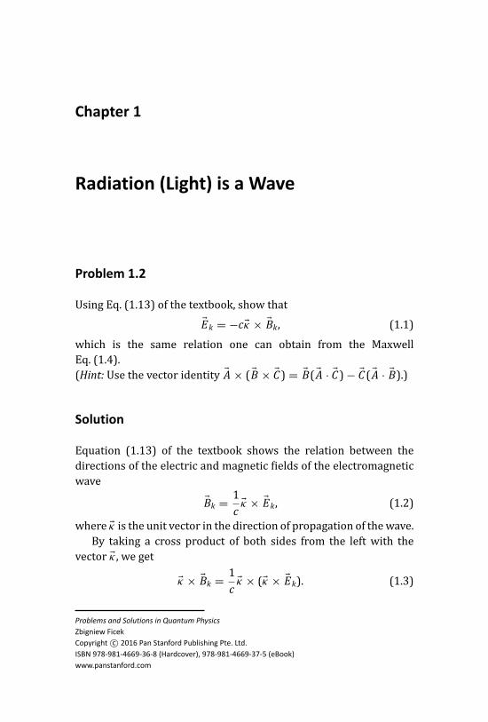
Problem 1.2
Using Eq. (1.13) of the textbook, show that
�Ek = −c�κ × �Bk, (1.1)
which is the same relation one can obtain from the Maxwell
Eq. (1.4).
(Hint: Use the vector identity �A × ( �B × �C ) = �B( �A · �C ) − �C ( �A · �B).)
Solution
Equation (1.13) of the textbook shows the relation between the
directions of the electric and magnetic fields of the electromagnetic
wave
�Bk = 1
c�κ × �Ek, (1.2)
where �κ is the unit vector in the direction of propagation of the wave.
By taking a cross product of both sides from the left with the
vector �κ , we get
�κ × �Bk = 1
c�κ × (�κ × �Ek). (1.3)
Problems and Solutions in Quantum PhysicsZbigniew FicekCopyright c© 2016 Pan Stanford Publishing Pte. Ltd.ISBN 978-981-4669-36-8 (Hardcover), 978-981-4669-37-5 (eBook)www.panstanford.com
March 18, 2016 13:47 PSP Book - 9in x 6in Zbigniew-Ficek-tutsol
2 Radiation (Light) is a Wave
Next, using the vector identity �A × ( �B × �C ) = �B( �A · �C ) − �C ( �A · �B),
we can write the right-hand side of the above equation as
1
c�κ × (�κ × �Ek) = 1
c
[�κ(�κ · �Ek) − �Ek(�κ · �κ)
]. (1.4)
Since �κ · �κ = 1 and the electric and magnetic fields are transverse
fields (�κ · �Ek = 0), we arrive at
�Ek = −c �κ × �Bk. (1.5)
This result for �Ek and that for �Bk, Eq. (1.2), show that both �Bk and�Ek of an electromagnetic wave are perpendicular to the direction of
propagation of the wave.
Problem 1.3
Show, using the divergence Maxwell equations, that the electromag-
netic waves in vacuum are transverse waves.
Solution
Consider an electromagnetic wave propagating in the z direction.
The wave is represented by the electric and magnetic fields of the
form
�E = �E0ei(ωt−kz),
�B = �B0ei(ωt−kz). (1.6)
The propagation of the wave is characterized by the frequency ω and
the wave number k.
When calculating divergences ∇ · �E and ∇ · �B , we get
∇ · �E = ∂ E x
∂x+ ∂ E y
∂y+ ∂ E z
∂z= 0 + 0 + ∂ E z
∂z,
∇ · �B = ∂ Bx
∂x+ ∂ By
∂y+ ∂ Bz
∂z= 0 + 0 + ∂ Bz
∂z. (1.7)
Since in vacuum ∇· �E = 0 and ∇· �B = 0 always in electromagnetism,
we have
∂ E z
∂z= 0 and
∂ Bz
∂z= 0. (1.8)
March 18, 2016 13:47 PSP Book - 9in x 6in Zbigniew-Ficek-tutsol
Radiation (Light) is a Wave 3
However, for the electric and magnetic fields of a plane wave,
∂ E z
∂z= −ikE z and
∂ Bz
∂z= −ikBz. (1.9)
Hence, the right-hand sides must be zero, which means that either
k = 0 or E z = 0 and Bz = 0, that both �E and �B are transverse to
the direction of propagation. Since k �= 0 for a propagating wave, the
wave is transverse in both �E and �B .
Problem 1.4
Calculate the energy of an electromagnetic wave propagating in one
dimension.
Solution
Consider a plane electromagnetic wave propagating in the zdirection in a vacuum with the electric field polarized in the xdirection:
�E = E0 sin(ωt − kz)i , (1.10)
where i is the unit vector in the x direction.
Having �E , we can calculate the magnetic field of the wave using
the Maxwell equation
∂ �B∂t
= −∇ × �E , (1.11)
and get
∂ �B∂t
= −∇ × �E = kE0 cos(ωt − kz) j . (1.12)
Integrating this equation, we find
�B = kE0
∫dt cos(ωt − kz) j = kE0
ωsin(ωt − kz) j . (1.13)
Since k/ω = 1/c, we finally obtain
�B = B0 sin(ωt − kz) j , (1.14)
where B0 = E0/c.
March 18, 2016 13:47 PSP Book - 9in x 6in Zbigniew-Ficek-tutsol
4 Radiation (Light) is a Wave
The energy of the electromagnetic field is determined by the
Poynting vector, defined as
�U = ε0c2 �E × �B = ε0c2 E0 B0 sin2(ωt − kz)k. (1.15)
Since B0 = E0/c, we have
�U = ε0cE 20 sin2(ωt − kz)k. (1.16)
Then, the average value 〈U 〉 of the magnitude of the Poynting vector
is
〈U 〉 = ε0cE 20〈sin2(ωt − kz)〉 = 1
2ε0cE 2
0 , (1.17)
where we have used the fact that 〈sin2(ωt − kz)〉 = 1/2.
March 18, 2016 13:47 PSP Book - 9in x 6in Zbigniew-Ficek-tutsol
Chapter 3
Blackbody Radiation
Problem 3.1
We have shown in Section 3.1 of the textbook that the number of
modes in the unit volume and the unit of frequency is
N = Nν = 1
Vd N(k)
dν= 8πν2
c3. (3.1)
In terms of the wavelength λ, we have shown that the number of
modes in the unit volume and the unit of wavelength is
N = Nλ = 8π
λ4. (3.2)
Explain, why it is not possible to obtain Nλ from Nν simply by using
the relation ν = c/λ.
Solution
The reason is that ν and λ are not linearly dependent on each other.
The frequency ν is inversely proportional to λ. Hence,
dν
dλ= − cλ2
. (3.3)
Problems and Solutions in Quantum PhysicsZbigniew FicekCopyright c© 2016 Pan Stanford Publishing Pte. Ltd.ISBN 978-981-4669-36-8 (Hardcover), 978-981-4669-37-5 (eBook)www.panstanford.com
March 18, 2016 13:47 PSP Book - 9in x 6in Zbigniew-Ficek-tutsol
6 Blackbody Radiation
Therefore, when going from the frequency space to the wavelength
space, we use the chain rule
1
Vd N(k)
dλ= 1
Vd N(k)
dν
dν
dλ= −8πν2
c2λ2. (3.4)
Then substituting ν = c/λ, we obtain
1
Vd N(k)
dλ= −8π
λ4. (3.5)
March 18, 2016 13:47 PSP Book - 9in x 6in Zbigniew-Ficek-tutsol
Chapter 4
Planck’s Quantum Hypothesis: Birth ofQuantum Theory
Problem 4.2
Using the Planck formula for Pn, show that
(a) The average number of photons is given by
〈n〉 = 1
ex − 1, (4.1)
where x = �ωkBT , and kB is the Boltzmann constant.
(b) Show that for large temperatures (T � 1), the average energy
is proportional to temperature, i.e., 〈E 〉 = kBT .
(c) Calculate 〈n2〉 and show that the ratio
α = 〈n2〉 − 〈n〉〈n〉2
= 2. (4.2)
Solution (a)
Using the Boltzmann formula for Pn and the definition of average,
we find
Problems and Solutions in Quantum PhysicsZbigniew FicekCopyright c© 2016 Pan Stanford Publishing Pte. Ltd.ISBN 978-981-4669-36-8 (Hardcover), 978-981-4669-37-5 (eBook)www.panstanford.com
March 18, 2016 13:47 PSP Book - 9in x 6in Zbigniew-Ficek-tutsol
8 Planck’s Quantum Hypothesis
〈n〉 =∞∑
n=0
nPn =∑∞
n=0 ne−nx∑∞n=0 e−nx
, (4.3)
where x = �ωkBT , and kB is the Boltzmann constant.
Since the ratio of successive terms in∑∞
n=0 e−nx is a constant,
e−(n+1)x
e−nx= e−x , (4.4)
the series∑∞
n=0 e−nx is a geometric series of the sum
∞∑n=0
e−nx = 1
1 − e−x. (4.5)
Hence
〈n〉 =∞∑
n=0
nPn = (1 − e−x) ∞∑
n=0
ne−nx . (4.6)
We can calculate the sum∑∞
n=0 ne−nx as follows. Denote
z =∞∑
n=0
e−nx = 1
1 − e−x. (4.7)
If we differentiate this expression with respect to x , we obtain
dzdx
= −∞∑
n=0
ne−nx = −e−x
(1 − e−x )2. (4.8)
Thus, we readily see that
∞∑n=0
ne−nx = e−x
(1 − e−x )2, (4.9)
and then
〈n〉 = (1 − e−x) ∞∑
n=0
ne−nx = (1 − e−x) e−x
(1 − e−x )2(4.10)
= e−x
1 − e−x= e−x ex
(1 − e−x )ex= 1
ex − 1. (4.11)
March 18, 2016 13:47 PSP Book - 9in x 6in Zbigniew-Ficek-tutsol
Planck’s Quantum Hypothesis 9
Solution (b)
Since En = n�ω, and using the solution to the part (a), we have
〈En〉 = 〈n〉�ω = �ω
ex − 1. (4.12)
For large temperatures T � 1, the parameter x 1, and then we
can expand the exponent ex into a Taylor series
ex ≈ 1 + x + . . . , (4.13)
from which we find that
ex − 1 ≈ x , (4.14)
which gives
〈En〉 = �ω
x= kBT . (4.15)
Thus, for large temperatures, the average energy of a quantum
radiation field agrees with that predicted by the Equipartition
theorem.
Solution (c)
From the definition of average and using the Boltzmann distribution
function, we find
〈n2〉 =∞∑
n=0
n2 Pn = (1 − e−x) ∞∑
n=0
n2e−nx , (4.16)
where, as before in (a), x = �ωkBT , and kB is the Boltzmann constant.
Since
dzdx
= −∞∑
n=0
ne−nx = −e−x
(1 − e−x )2, (4.17)
we take a derivative over x of both sides of the above equation and
obtain
d2zdx2
=∞∑
n=0
n2e−nx = e−x (1 + e−x )
(1 − e−x )3. (4.18)
March 18, 2016 13:47 PSP Book - 9in x 6in Zbigniew-Ficek-tutsol
10 Planck’s Quantum Hypothesis
Hence
〈n2〉 = e−x (1 + e−x )
(1 − e−x )2= e2x e−x (1 + e−x )
e2x (1 − e−x )2(4.19)
= (ex + 1)
(ex − 1)2. (4.20)
From the relation
〈n〉 = 1
ex − 1, (4.21)
we find that
ex = 1 + 1
〈n〉 , (4.22)
and after substituting this result into Eq. (4.20), we obtain
〈n2〉 = 2〈n〉 + 1
〈n〉 〈n〉2 = 〈n〉 + 2〈n〉2. (4.23)
Hence
α = 〈n2〉 − 〈n〉〈n〉2
= 〈n〉 + 2〈n〉2 − 〈n〉〈n〉2
= 2. (4.24)
The parameter α is known in statistical physics as a measure of
correlations (distribution) between photons in a radiation field. The
value α = 2 means that in a thermal field, the correlations between
photons are large. In other words, the photons group together (move
in large groups). This effect is often called photon bunching.
Problem 4.3
Suppose that photons in a radiation field have a Poisson distribution
defined as
Pn = 〈n〉n
n!e−〈n〉. (4.25)
Calculate the variance of the number of photons defined as σn =〈n2〉 − 〈n〉2 and show that the ratio α = 1.
March 18, 2016 13:47 PSP Book - 9in x 6in Zbigniew-Ficek-tutsol
Planck’s Quantum Hypothesis 11
Solution
With the Poisson distribution of photons
Pn = 〈n〉n
n!e−〈n〉, (4.26)
the average number of photons is given by
〈n〉 =∑
n
nPn =∑
n
n 〈n〉n
n!e−〈n〉
= 〈n〉 e−〈n〉 ∑n
〈n〉n−1
(n − 1)!= 〈n〉 , (4.27)
where we have used the fact that∑n
〈n〉n−1
(n − 1)!= e〈n〉, (4.28)
i.e., the above sum is a Taylor expansion of e〈n〉.Similarly, we can calculate 〈n2〉 as
〈n2〉 =∑
n
n2 Pn =∑
n
n2e−〈n〉 〈n〉n
n!= 〈n〉 e−〈n〉 ∑
n
n 〈n〉n−1
(n − 1)!. (4.29)
To proceed further with the sum over n, we change the variable by
substituting n − 1 = k and obtain
〈n2〉 = 〈n〉 e−〈n〉{∑
k
k 〈n〉k
k!+∑
k
〈n〉k
k!
}. (4.30)
The two sums over k are easy to evaluate, and finally we obtain
〈n2〉 = 〈n〉2 + 〈n〉 . (4.31)
Thus, the variance of photons in a field with the Poisson distribu-
tions is given by
σn = 〈n2〉 − 〈n〉2 = 〈n〉 , (4.32)
and then we readily find from the definition of α that
α = 1. (4.33)
The value of α = 1 means that photons in the field with Poisson
distribution are independent of each other. Such a field is called a
coherent field.
March 18, 2016 13:47 PSP Book - 9in x 6in Zbigniew-Ficek-tutsol
12 Planck’s Quantum Hypothesis
Problem 4.5
Show that at the wavelength λmax, the intensity I (λ) calculated from
Planck’s formula has its maximum
I (λmax) ≈ 170π(kBT )5
(hc)4, (4.34)
where kB is the Boltzmann constant.
Solution
Consider Planck’s formula in terms of wavelength
I (λ) = 8πhcλ5(
ehc/λkBT − 1) . (4.35)
Since Planck’s formula has its maximum at
λmax = hc4.9651kBT
, (4.36)
we find the maximum value of I (λmax) as
I (λmax) = 8πhc(hc)5
(4.9651kBT )5 1
e4.9651 − 1
= π(kBT )5
(hc)4
8 × (4.9651)5
e4.9651 − 1
≈ π(kBT )5
(hc)4170 = 170π(kBT )5
(hc)4. (4.37)
Problem 4.6
(a) Derive the Wien displacement law by solving the equation
d I (λ)/dλ = 0.
(Hint: Set hc/λkBT = x and show that d I/dx leads to the
equation e−x = 1 − 15
x . Then show that x = 4.956 is the
solution.)
(b) In part (a), we have obtained λmax by setting d I (λ)/dλ = 0.
Calculate νmax from the Planck formula by setting d I (ν)/dν = 0.
March 18, 2016 13:47 PSP Book - 9in x 6in Zbigniew-Ficek-tutsol
Planck’s Quantum Hypothesis 13
Is it possible to obtain νmax from λmax simply by using λmax =c/νmax? Note, νmax is the frequency at which the intensity of the
emitted radiation is maximal.
Solution (a)
In the Planck formula
I (λ) = 8πhcλ5(
ehc/λkBT − 1) , (4.38)
we substitute for
hcλkBT
= x , (4.39)
and obtain
I (x) = Ax5
(ex − 1), (4.40)
where
A = 8πhc(kBT )5
(hc)5(4.41)
is a constant independent of λ.
We find the maximum of I (x) by solving the equation
d I (x)
dx= 0. (4.42)
Thus
d I (x)
dx= A
5x4 (ex − 1) − x5ex
(ex − 1)2= A
x4 [5 (ex − 1) − xex ]
(ex − 1)2.
(4.43)
Hence
d I (x)
dx= 0 when x = 0 or 5 (ex − 1) − xex = 0.
(4.44)
The root x = 0 is unphysical as it would correspond to T → ∞, so
we will focus on the solution to the exponent-type equation, which
can be written as
e−x = 1 − 1
5x . (4.45)
March 18, 2016 13:47 PSP Book - 9in x 6in Zbigniew-Ficek-tutsol
14 Planck’s Quantum Hypothesis
This equation cannot be solved exactly. Therefore, we will apply an
approximate method.
One can see that there are two roots of the above equation: x = 0
(exact root) and an approximate root x ≈ 5 (as e−5 ≈ 0). The root
x = 0 is unphysical as it would correspond to T → ∞, so we will
focus on the root x ≈ 5.
How to estimate the exact root if we know an approximate root?
Let x0 be close to the exact root of F (x) and let x0 + x be the
exact root. Then, using a Taylor expansion, we can write
F (x0 + x) = F (x0) + F ′x = 0, (4.46)
where
F ′(x0) = d F (x)
dx|x=x0
. (4.47)
Hence, assuming that x0 is a root of the equation, the error in the
estimation of the exact root is equal to
x = − F (x0)
F ′(x0). (4.48)
Let
F (x) = 5 (ex − 1) − xex . (4.49)
Then
F ′(x) = 5ex − ex − xex = (4 − x)ex . (4.50)
Thus, for x ≡ x0 = 5:
F (5) = 5(
e5 − 1)− 5e5 = −5,
F ′(5) = −e5 = −148.41, (4.51)
from which we find the error in the estimation that x0 = 5 is the root
of the equation
x = − 5
e5= −0.0336. (4.52)
Take x = 4.9651. In this case
F (4.9651) = 0.002 , F ′(4.9651) = −138.32, (4.53)
which gives x = −0.00001.
Take x = 4.956. In this case
F (4.956) = 1.252, F ′(4.956) = −135.77, (4.54)
which gives x = −0.009.
Thus, x = 4.9651 is very close to the exact root of the equation.
Having the value of x at which I (λ) is maximal, we find from
hc/λkBT = x the Wien displacement law
λmaxT = hc4.9651kB
= constant. (4.55)
March 18, 2016 13:47 PSP Book - 9in x 6in Zbigniew-Ficek-tutsol
Planck’s Quantum Hypothesis 15
Solution (b)
Consider the energy density distribution in terms of frequency
I (ν) = N(ν)〈E 〉, (4.56)
where N(ν) = 8πν2/c3 is the number of modes per unit volume and
unit frequency (see Section 3.1 of the textbook for the derivation),
and 〈E 〉 is the average energy of a single mode.
Thus, using Planck’s quantum hypothesis, the energy density
distribution in terms of frequency can be written as
I (ν) = 8πν2
c3
hν
ehν/kBT − 1= 8πh
c3
ν3
ehν/kBT − 1. (4.57)
Substituting for hν/kBT = x , we can write the energy density
distribution as
I (ν) ≡ I (x) = 8πhc3
( kBTh x
)3
ex − 1= A
x3
ex − 1, (4.58)
where A = 8π(kBT )3/(c3h2).
We find the maximum of I (x) by solving the equation
d I (x)
dx= 0. (4.59)
Thus
d I (x)
dx= A
3x2 (ex − 1) − x3ex
(ex − 1)2= A
x2 [3 (ex − 1) − xex ]
(ex − 1)2. (4.60)
Hence
d I (x)
dx= 0 when 3 (ex − 1) − xex = 0. (4.61)
This equation cannot be solved exactly. Therefore, we will apply an
approximate method outlined in part (a).
One can see that there are two roots of the above equation: x = 0
(exact root) and an approximate root x ≈ 3 ( as e3 � 1). The root
x = 0 is unphysical as it would correspond to T → ∞, so we will
focus on the root x ≈ 3.
Let
F (x) = 3 (ex − 1) − xex . (4.62)
March 18, 2016 13:47 PSP Book - 9in x 6in Zbigniew-Ficek-tutsol
16 Planck’s Quantum Hypothesis
Then
F ′(x) = 3ex − ex − xex = (2 − x)ex . (4.63)
Thus, for x ≡ x0 = 3:
F (3) = 3(
e3 − 1)− 3e3 = −3,
F ′(3) = −e3 = −20.085, (4.64)
from which we find the error in the estimation that x0 = 3 is the root
of the equation
x = − −3
−e3= −0.15. (4.65)
Take x = 2.85. In this case
F (2.85) = −0.41, F ′(2.85) = −14.69, (4.66)
which gives x = −0.028.
Take x = 2.82. In this case
F (2.82) = 0.02, F ′(2.82) = −13.757, (4.67)
which gives x = −0.0014.
Thus, x = 2.82 is a better root.
Hence, for x = 2.82, the corresponding frequency is
νmax = kBTh
x = 2.82kB
hT . (4.68)
In the Tutorial Problem 4.6(a), we found that
λmax = hc4.9651kBT
. (4.69)
If we apply the relation λmax = c/νmax, we obtain for νmax
νmax = 4.9651kB
hT . (4.70)
This result differs from that in Eq. (4.68), and in this case, νmax is
larger than that calculated exactly.
The reason is that λ and ν are not linearly dependent quantities,
λ = c/ν, and then the densities of modes N(λ) and N(ν) are not
linear functions.
March 18, 2016 13:47 PSP Book - 9in x 6in Zbigniew-Ficek-tutsol
Planck’s Quantum Hypothesis 17
Problem 4.7
Derive the Stefan–Boltzmann law evaluating the integral in
Eq. (4.15) of the textbook.
Hint: It is convenient to evaluate the integral by introducing a
dimensionless variable
x = hcλkBT
. (4.71)
Solution
To actually evaluate Eq. (4.15), it is convenient to simplify Planck’s
formula
I (λ) = 8πhcλ5(
ehc/λkB T − 1) (4.72)
by introducing a dimensionless variable
x = hcλkBT
. (4.73)
When we change the variable in Planck’s formula from λ to x :
λ = hckBT
1
xso that dλ = − hc
kBT1
x2dx , (4.74)
we find that in terms of x , the total intensity I becomes
I = c4
∫ ∞
0
I (λ)dλ = c4
∫ ∞
0
dx8πhc(
hckBT
)5
x5
ex − 1
hckBT x2
=∫ ∞
0
dx2πhc2(
hckBT
)4
x3
ex − 1= 2πhc2
(kBThc
)4 ∫ ∞
0
dxx3
ex − 1.
(4.75)
Since ∫ ∞
0
x3dxex − 1
= π4
15, (4.76)
we finally obtain
I = 2πhc2
(kBThc
)4π4
15= σ T 4, (4.77)
March 18, 2016 13:47 PSP Book - 9in x 6in Zbigniew-Ficek-tutsol
18 Planck’s Quantum Hypothesis
where
σ = 2π5k4B
15h3c2= 5.67 × 10⁻⁸ [W/m2 · K4]. (4.78)
The constant σ determined from experimental results agrees
perfectly with the above value derived from Planck’s formula.
Problem 4.10
Consider Compton scattering.
(a) Show that E/E , the fractional change in photon energy in the
Compton effect, satisfies
EE
= hν ′
m0c2(1 − cos α) , (4.79)
where ν ′ is the frequency of the scattered photon and E =E − E ′.
(b) Show that the relation between the directions of motion of the
scattered photon and the recoil electron in Compton scattering
is
cotα
2=(
1 + hν
m0c2
)tan θ , (4.80)
where α is the angle of the scattered photon, θ is the angle of the
recoil electron, and ν is the frequency of the incident light.
Solution (a)
Use the Compton formula written in terms of the momenta of the
incident ( p) and scattered ( p′) photons
p − p′ = pp′
m0c(1 − cos α) . (4.81)
Since p = E/c, we can write the above formula in terms of the
energies of the incident (E ) and scattered (E ′) photons
E − E ′ = E E ′
m0c2(1 − cos α) . (4.82)
Introducing a notation E = E − E ′, and using E ′ = hν ′, we obtain
EE
= hν ′
m0c2(1 − cos α) . (4.83)
March 18, 2016 13:47 PSP Book - 9in x 6in Zbigniew-Ficek-tutsol
Planck’s Quantum Hypothesis 19
Solution (b)
As in Solution (a), consider the Compton formula in terms of the
momenta of the incident and scattered photons
p − p′ = pp′
m0c(1 − cos α) . (4.84)
We will express the momentum of the scattered photons, p′, in
terms of the momentum p of the incident photons using the
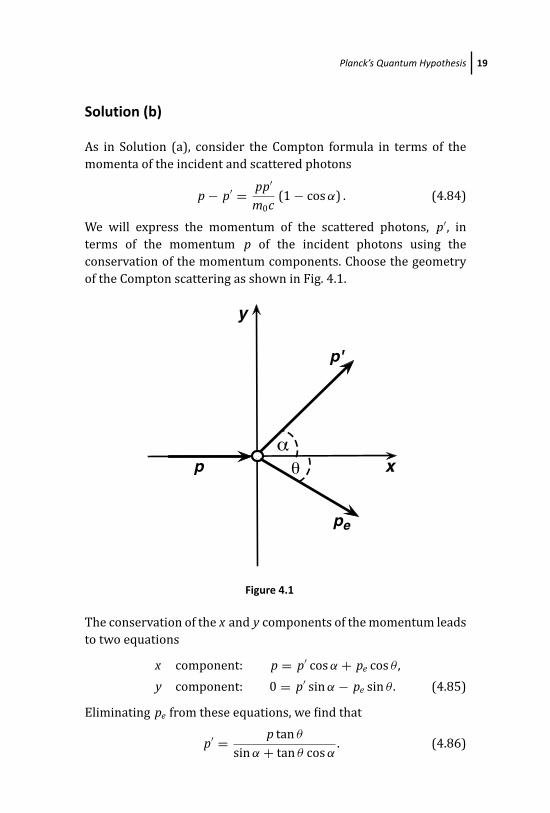
conservation of the momentum components. Choose the geometry
of the Compton scattering as shown in Fig. 4.1.
p
p'
pe
x
y
αθ
Figure 4.1
The conservation of the x and y components of the momentum leads
to two equations
x component: p = p′ cos α + pe cos θ ,
y component: 0 = p′ sin α − pe sin θ . (4.85)
Eliminating pe from these equations, we find that
p′ = p tan θ
sin α + tan θ cos α. (4.86)
March 18, 2016 13:47 PSP Book - 9in x 6in Zbigniew-Ficek-tutsol
20 Planck’s Quantum Hypothesis
Substituting this into Eq. (4.84), we obtain
p(
1 − tan θ
sin α + tan θ cos α
)= p2
m0ctan θ
(sin α + tan θ cos α)(1 − cos α) ,
(4.87)
which can be written as
sin α
1 − cos α=(
pm0c
+ 1
)tan θ . (4.88)
Since
sin α
1 − cos α= cot
α
2and p = E
c= hν
c, (4.89)
we finally obtain
cotα
2=(
1 + hν
m0c2
)tan θ . (4.90)
This formula shows that one can test the Compton effect by
measuring the angles α and θ instead of measuring the wavelength
λ′ of the scattered photons.
March 18, 2016 13:47 PSP Book - 9in x 6in Zbigniew-Ficek-tutsol
Chapter 5
Bohr Model
Problem 5.2
Suppose that the electron is a spherical shell of radius re and all the
electron’s charge is evenly distributed on the shell. Using the formula
for the energy of a charged shell, calculate the classical electron
radius. Compare the size of the electron with the size of an atomic
nucleus.
Solution
We know from classical electromagnetism that the energy of a
charged shell is
E = e2
4πε0re
. (5.1)
Since E = mc2, we find
re = e2
4πε0mc2= 2.82 × 10⁻¹⁵ m. (5.2)
This is the allowed classical electron radius. It is about the size of an
atomic nucleus. The size of the electron cannot be smaller than this;
otherwise, the electron’s mass would be larger.
Problems and Solutions in Quantum PhysicsZbigniew FicekCopyright c© 2016 Pan Stanford Publishing Pte. Ltd.ISBN 978-981-4669-36-8 (Hardcover), 978-981-4669-37-5 (eBook)www.panstanford.com
March 18, 2016 13:47 PSP Book - 9in x 6in Zbigniew-Ficek-tutsol
22 Bohr Model
However, according to experiments, the electron is smaller, and
yet its mass is not larger. Thus, classical electromagnetism must be
revised for elementary particles.
Problem 5.4
Show that in the Bohr atom model, the electron’s orbits in a
hydrogen-like atom are quantized with the radius r = n2ao/Z ,
where ao = 4πε0�2/me2 is the Bohr radius, n = 1, 2, . . . , and Z is
atomic number. Z = 1 refers to a hydrogen atom, Z = 2 to a helium
(He+) ion, and so on.
Solution
From the classical equation of motion for the electron in a hydrogen-
like atom (Coulomb force = centripetal force)
Z e2
4πε0r2= m
v2
r, (5.3)
we find the velocity of the electron
v =√
Z e2
4πε0mr. (5.4)
Bohr postulated that the angular momentum of the electron is
quantized with
L = n� , n = 1, 2, 3, . . .
(� = h
2π
). (5.5)
Since
L = mvr =√
Z me2r4πε0
, (5.6)
we obtain
Z me2r4πε0
= n2�
2, (5.7)
from which we find
r = n2 ao
Z, where ao = 4πε0�
2
me2. (5.8)
March 18, 2016 13:47 PSP Book - 9in x 6in Zbigniew-Ficek-tutsol
Bohr Model 23
Problem 5.5
The magnetic dipole moment �μ of a current loop is defined by �μ =I �S , where I is the current and �S = S�n is the area of the loop, with �n,
the unit vector, normal to the plane of the loop. A current loop may
be represented by a charge e rotating at constant speed in a circular
orbit. Use the classical model of the orbital motion of the electron
and Bohr’s quantization postulate to show that the magnetic dipole
moment of the loop is quantized such that
μ = n mB , n = 1, 2, 3, . . . , (5.9)
where mB = e�/2m is the Bohr magneton, and m is the mass of the
electron.
Solution
Denote the radius of the electron’s orbit by r and the linear velocity
of the electron by v = ωr , where ω is the angular velocity. Then the
period of revolution is
T = 2π
ω= 2πr
v. (5.10)
Hence, the current induced by the revolting electron is
I = eT
= ev2πr
. (5.11)
We know from electromagnetism that current produces a magnetic
field and a current loop closing some area creates a magnetic
moment. The magnetic moment is equal to the product of the area
of the plane loop and the magnitude of the circulating current:
�μ = I �S = I Sn, (5.12)
where S = πr2 is the area closed by the loop (the orbit of the
revolting electron), n is the unit vector perpendicular to the plane
of the loop and oriented along the direction set by the right-hand
rule.
Thus
�μ = ev2πr
πr2n = 1
2evrn. (5.13)
March 18, 2016 13:47 PSP Book - 9in x 6in Zbigniew-Ficek-tutsol
24 Bohr Model
From the definition of the angular momentum
�L = �p × �r = mvrn, (5.14)
where �p = m�v , we find that
�μ = 1
2evrn = e
2m�L. (5.15)
Since
L = n�, (5.16)
we find that
�μ = ne�
2mn = n mBn, (5.17)
where mB = e�/2m = 9.27 × 10⁻²⁴ [A·m2] is the Bohr magneton.
Problem 5.6
Consider an experiment. A student is at a distance of 10 m from a
light source whose power is P = 40 W.
(a) How many photons strike the student’s eye if the wavelength
of light is 589 nm (yellow light) and the radius of the pupil (a
variable aperture through which light enters the eye) is 2 mm.
(b) At what distance from the source, only one photon would strike
the student’s eye.
Solution (a)
The intensity of light at a distance of 10 m from the source is
I = P4πr2
= 40
4π(10)2= 0.032
[W
m2
]. (5.18)
Energy of a single photon of wavelength λ = 589 nm is
E = hν = hcλ
= 6.63 × 10−34 × 3 × 108
589 × 10−9= 0.034 × 10⁻¹⁷ [J] .
(5.19)
The rate at which energy is absorbed by the eye is given by
R = I A = 0.032 × π × (2 × 10⁻³)2 = 402.1 × 10⁻⁹
[J
s
], (5.20)
where A is the area of the pupil.
March 18, 2016 13:47 PSP Book - 9in x 6in Zbigniew-Ficek-tutsol
Bohr Model 25
Hence, we find that the number of photons striking the eye per
second is given by
n = RE
= 402.1 × 10⁻⁹
0.034 × 10−17= 11,826.5×108 ≈ 12×1011
[photons
s
].
(5.21)
Solution (b)
We have to find the distance at which the rate of absorption of light
per second is equal to the energy of a single photon, i.e.,
R = I A = E . (5.22)
Since I = P/(4πr2), we have
P A4πr2
= E , (5.23)
from which we find
r2 = P A4π E
. (5.24)
Hence
r =√
P A4π E
=√
40 × π × (2 × 10⁻³)2
4π × 0.034 × 10−17
=√
118 × 1012 ≈ 11 × 106 [m] = 11 × 103 [km]. (5.25)

This page intentionally left blankThis page intentionally left blank
March 18, 2016 13:47 PSP Book - 9in x 6in Zbigniew-Ficek-tutsol
Chapter 6
Duality of Light and Matter
Problem 6.3
Determine where a particle is most likely to be found whose wave
function is given by
� (x) = 1 + i x1 + i x2
. (6.1)
Solution
The probability density of finding the particle at a point x is given by
|� (x)|2 = � (x) �∗ (x) = 1 + i x1 + i x2
1 − i x1 − i x2
= 1 + x2
1 + x4. (6.2)
The particle is most likely to be found at points for which
d|�|2/dx = 0. Since
d |�|2
dx= 2x(1 + x4) − 4x3(1 + x2)
(1 + x4)2, (6.3)
we find that d|�|2/dx = 0 when
2x(1 + x4) − 4x3(1 + x2) = 0. (6.4)
Problems and Solutions in Quantum PhysicsZbigniew FicekCopyright c© 2016 Pan Stanford Publishing Pte. Ltd.ISBN 978-981-4669-36-8 (Hardcover), 978-981-4669-37-5 (eBook)www.panstanford.com
March 18, 2016 13:47 PSP Book - 9in x 6in Zbigniew-Ficek-tutsol
28 Duality of Light and Matter
This equation can be simplified to
x4 + 2x2 − 1 = 0, (6.5)
which, after substituting x2 = z, reduces to a quadratic equation
z2 + 2z − 1 = 0, (6.6)
whose the roots are
z1 = −1 +√
2 and z2 = −1 −√
2. (6.7)
Thus d|�|2/dx = 0 when
x21 = −1 +
√2 and x2
2 = −1 −√
2. (6.8)
Since x2 > 0, the only solution we can accept is
x1 = ±√
−1 +√
2. (6.9)
Problem 6.4
The wave function of a free particle at t = 0 is given by
�(x , 0) =⎧⎨⎩
0 x < −b,
A −b ≤ x ≤ 3b,
0 x > 3b.
(6.10)
(a) Using the fact that the probability is normalized to one, i.e.,∫ +∞
−∞|�(x , 0)|2dx = 1, (6.11)
find the constant A. (You can assume that A is real.)
(b) What is the probability of finding the particle within the
interval x ∈ [0, b] at time t = 0?
Solution (a)
The constant A is found from the normalization condition, which can
be written as
1 =∫ +∞
−∞|�|2dx =
∫ −b
−∞|�|2dx +
∫ 3b
−b|�|2dx +
∫ +∞
3b|�|2dx
= 0 +∫ 3b
−b|�|2dx + 0 = A2
∫ 3b
−bdx = 4bA2. (6.12)
March 18, 2016 13:47 PSP Book - 9in x 6in Zbigniew-Ficek-tutsol
Duality of Light and Matter 29
Hence
A = 1
2√
b. (6.13)
Solution (b)
The probability of finding the particle within the interval x ∈ [0, b]
at time t = 0 is given by∫ b
0
|�|2dx = A2
∫ b
0
dx = 1
4bb = 1
4. (6.14)
Problem 6.5
The state of a free particle at t = 0 confined between two walls
separated by a is described by the following wave function:
�(x , 0) = �max sin(nπ
ax)
, 0 ≤ x ≤ a,
�(x , 0) = 0, x > a, and x < 0. (6.15)
(a) Find the amplitude �max using the normalization condition.
(b) What is the probability density of finding the particle at x =0, a/2, and a. How does the result depend on n?
(c) Calculate the probability of finding the particle in the regionsa2
≤ x ≤ a and 3a4
≤ x ≤ a, for n = 1 and n = 2.
Solution (a)
From the normalization condition, we find
1 =∫ +∞
−∞|�|2dx =
∫ 0
−∞|�|2dx +
∫ a
0
|�|2dx +∫ +∞
a|�|2dx
= 0 +∫ a
0
|�|2dx + 0 = |�max|2
∫ a
0
sin2(nπ
ax)
dx
= 1
2|�max|2
∫ a
0
[1 − cos
(2nπ
ax)]
dx
= 1
2|�max|2
[x − a
2nπsin
(2nπ
ax)]a
0
= a2
|�max|2, (6.16)
March 18, 2016 13:47 PSP Book - 9in x 6in Zbigniew-Ficek-tutsol
30 Duality of Light and Matter
as sin (2nπ) = sin(0) = 0. Hence
|�max| =√
2
a. (6.17)
Solution (b)
From the definition of the probability density, Pd = |�(x)|2, we find
Pd = 2
asin2
(nπ
ax)
. (6.18)
Thus, at x = 0, the probability density Pd = 0 is independent of n.
Similarly, at x = a, the probability density Pd = 0 is independent
of n.
At x = a/2
Pd = 2
asin2
(nπ
a
). (6.19)
Hence, for odd n (n = 1, 3, 5, . . .), the probability density is
maximum (equal to 2/a), whereas for even n (n = 2, 4, 6, . . .), the
probability density Pd = 0.
Solution (c)
The probability of finding the particle in the region a2
≤ x ≤ a is
given by
P =∫ a
a/2
|�|2dx = |�max|2
∫ a
a/2
sin2(nπ
ax)
dx
= 1
2|�max|2
∫ a
a/2
[1 − cos
(2nπ
ax)]
dx
= 1
a
[x − a
2nπsin
(2nπ
ax)]a
a/2
= 1
2, (6.20)
for both n = 1 and n = 2, as sin (2nπ) = sin(nπ) = 0 for all n.
March 18, 2016 13:47 PSP Book - 9in x 6in Zbigniew-Ficek-tutsol
Duality of Light and Matter 31
Similarly as above, we find that the probability of finding the
particle in the region 3a4
≤ x ≤ a is given by
P =∫ a
3a/4
|�|2dx = |�max|2
∫ a
3a/4
sin2(nπ
ax)
dx
= 1
2|�max|2
∫ a
3a/4
[1 − cos
(2nπ
ax)]
dx
= 1
a
[x − a
2nπsin
(2nπ
ax)]a
3a/4
= 1
4+ 1
2nπsin
(3
2nπ
).
(6.21)
Now since sin(
32
nπ) = −1 for n = 1, and sin
(32
nπ) = 0 for n = 2,
we have the result
P = 1
4
(1 − 2
π
)for n = 1,
P = 1
4for n = 2. (6.22)
Problem 6.6
The time-independent wave function of a particle is given by
�(x) = Ae−|x|/σ , (6.23)
where A and σ are constants.
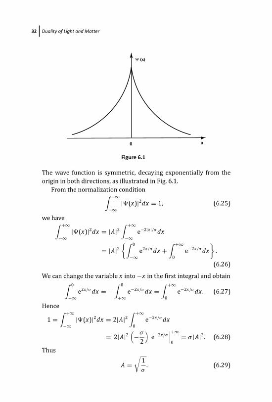
(a) Sketch this function and find A in terms of σ such that �(x) is
normalized.
(b) Find the probability that the particle will be found in the region
−σ ≤ x ≤ σ .
Solution (a)
The wave function �(x) can be written as
�(x) =⎧⎨⎩
Aex/σ for x < 0,
Ae−x/σ for x ≥ 0.
(6.24)
March 18, 2016 13:47 PSP Book - 9in x 6in Zbigniew-Ficek-tutsol
32 Duality of Light and Matter
x
Ψ (x)
0
Figure 6.1
The wave function is symmetric, decaying exponentially from the
origin in both directions, as illustrated in Fig. 6.1.
From the normalization condition∫ +∞
−∞|�(x)|2dx = 1, (6.25)
we have∫ +∞
−∞|�(x)|2dx = |A|2
∫ +∞
−∞e−2|x|/σ dx
= |A|2
{∫ 0
−∞e2x/σ dx +
∫ +∞
0
e−2x/σ dx}
.
(6.26)
We can change the variable x into −x in the first integral and obtain∫ 0
−∞e2x/σ dx = −
∫ 0
+∞e−2x/σ dx =
∫ +∞
0
e−2x/σ dx . (6.27)
Hence
1 =∫ +∞
−∞|�(x)|2dx = 2|A|2
∫ +∞
0
e−2x/σ dx
= 2|A|2(−σ
2
)e−2x/σ
∣∣∣+∞
0= σ |A|2. (6.28)
Thus
A =√
1
σ. (6.29)
March 18, 2016 13:47 PSP Book - 9in x 6in Zbigniew-Ficek-tutsol
Duality of Light and Matter 33
Solution (b)
The probability of finding the particle in the region −σ ≤ x ≤ σ is
P =∫ σ
−σ
|�(x)|2dx = |A|2
∫ σ
−σ
e−2|x|/σ dx
= |A|2
{∫ 0
−σ
e2x/σ dx +∫ σ
0
e−2x/σ dx}
= 2|A|2
∫ σ
0
e−2x/σ dx
= 2|A|2(−σ
2
)e−2x/σ
∣∣∣σ0
= − (e−2 − 1
) = 1 − e−2 = 0.856.
(6.30)
Thus, there is about a 86% chance that the particle will be found in
the region −σ ≤ x ≤ σ .
Problem 6.7
We have calculated the phase velocity u using the relativistic formula
for energy. Calculate the phase velocity for the non-relativistic case.
Does the relativistic result for u tends to the corresponding non-
relativistic result as the velocity of the particle becomes small
compared to the speed of light?
Solution
In the non-relativistic case, the energy of the particle is given by
E = p2
2m, (6.31)
where p is the momentum of the particle.
Since p = �k and E = �ω, we have
E = p2
2m= �
2
2mk2 = �ω. (6.32)
Thus, in the non-relativistic case
ω = �
2mk2. (6.33)
March 18, 2016 13:47 PSP Book - 9in x 6in Zbigniew-Ficek-tutsol
34 Duality of Light and Matter
With this relation between ω and k, we find that the phase velocity
is
u = ω
k= �
2mk, (6.34)
and the group velocity is
vg = dω
dk= �
mk = p
m= v . (6.35)
Therefore,
u = 1
2vg = 1
2v . (6.36)
In the relativistic case
u = c2
vg
= c2
v. (6.37)
Thus, the relativistic case does not tend to the non-relativistic case
when v c. Normally, a relativistic result in physics tends to
the corresponding non-relativistic result as the velocity involved
becomes small compared to the speed of light. This is clearly not the
case for the above two expressions for phase velocity. The reason is
that the expression for the relativistic energy
E 2 = p2c2 + (m0c2)2 (6.38)
includes the rest-mass term, m0c2, whereas the expression for the
non-relativistic energy E = p2/2m does not include the rest-mass
term.
Problem 6.8
We know that the group velocity vg of the wave packet of a particle
of mass m is equal to the velocity v of the particle. Show that the total
energy of the particle is E = �ω, the same which holds for photons.
Solution
From the definition of momentum
�p = m�v , (6.39)
March 18, 2016 13:47 PSP Book - 9in x 6in Zbigniew-Ficek-tutsol
Duality of Light and Matter 35
and the fact that the velocity of the particle �v = �vg and �p = ��k, we
have
m�vg = ��k. (6.40)
Using the definition of the group velocity, which in three dimensions
can be written as
�vg = ∇kω, (6.41)
where
∇kω = ∂ω
∂kx
�i + ∂ω
∂ky
�j + ∂ω
∂kz
�k (6.42)
is the gradient over the components of �k (kx , ky , kz), we have
m∇kω = ��k. (6.43)
Integrating this equation over k, we obtain
mω = �
2
(k2
x + k2y + k2
z
)+ C , (6.44)
where C is a constant.
Hence, multiplying both sides by � and dividing by m, we obtain
�ω = �2
2mk2 + A , (6.45)
where A = �C/m is a constant.
Since �2k2 = p2, we see that the right-hand side of the above
equation is the total energy E of the particle. Thus,
�ω = E , (6.46)
which is the same that holds for photons.
Problem 6.11
The time required for a wave packet to move the distance equal to
the width of the wave packet is t = x/vg, where x is the width
of the wave packet. Show that the time t and the uncertainty in the
energy of the particle satisfy the uncertainty relation
Et = h, (6.47)
where E = �ω.
March 18, 2016 13:47 PSP Book - 9in x 6in Zbigniew-Ficek-tutsol
36 Duality of Light and Matter
Solution
Since
x = vgt = ω
kt, (6.48)
we find that the uncertainty relation
xk = 2π, (6.49)
can be written as
xk = ω
ktk = ωt = 2π. (6.50)
Multiplying both sides of the above equation by �, we obtain
�ωt = 2π� = h. (6.51)
Since E = �ω, we finally obtain the energy and time uncertainty
relation
Et = h. (6.52)
In the above relation, E is the uncertainty in our knowledge of the
energy E of a system and t is the time interval characteristic of the
rate of changes in the system’s energy.
Problem 6.12
The amplitude A(k) of the wave function
�(x , t) =∫ +∞
−∞A(k)ei(kx−ωkt)dk (6.53)
is given by
A(k) =⎧⎨⎩
1 for k0 − 12k ≤ k ≤ k0 + 1
2k,
0 for k > k0 + 12k and k < k0 − 1
2k.
(6.54)
(a) Show that the wave function can be written as
�(x , t) = sin zz
k ei(k0 x−ω0t), (6.55)
where z = 12k(x − vgt).
(b) Sketch the function f (z) = sin z/z and find the width of the
main maximum of f (z).
(Hint: For f (z), one might define a suitable width as the spacing
between its first two zeros.)
March 18, 2016 13:47 PSP Book - 9in x 6in Zbigniew-Ficek-tutsol
Duality of Light and Matter 37
Solution (a)
With the shape of the amplitude A(k):
A(k) =⎧⎨⎩
1 for k0 − 12k ≤ k ≤ k0 + 1
2k,
0 for k > k0 + 12k, and k < k0 − 1
2k,
(6.56)
the wave packet has the form
�(x , t) =∫
kA(k)ei(kx−ωkt)dk =
∫ k0+ 12k
k0− 12k
ei(kx−ωkt)dk. (6.57)
Taking k = k0+β , and expanding ωk into a Taylor series about k = k0,
we get
ωk = ωk0+β = ω0 +(
dω
dβ
)k0
β + 1
2
(d2ω
dβ2
)k0
β2 + . . . , (6.58)
where ω0 = ωk0.
If we take only the first two terms of the series and substitute to
�(x , t), we obtain
�(x , t) = ei(k0 x−ω0t)
∫ 12k
− 12k
dβeiβ(x−vgt), (6.59)
where vg =(
dωdβ
)k0
is the group velocity of the packet.
Performing the integration, we obtain
�(x , t) = ei(k0 x−ω0t) eiβ(x−vgt)
i(x − vgt)
∣∣∣∣12k
− 12k
= ei(k0 x−ω0t)
[ei(x−vgt) 1
2k − e−i(x−vgt) 1
2k]
i(x − vgt)
= 2ei(k0 x−ω0t)
(x − vgt)sin
[1
2k(x − vgt)
]= sin z
zk ei(k0 x−ω0t),
(6.60)
where z = 12k(x − vgt).
March 18, 2016 13:47 PSP Book - 9in x 6in Zbigniew-Ficek-tutsol
38 Duality of Light and Matter
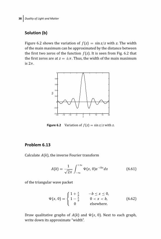
Solution (b)
Figure 6.2 shows the variation of f (z) = sin z/z with z. The width
of the main maximum can be approximated by the distance between
the first two zeros of the function f (z). It is seen from Fig. 6.2 that
the first zeros are at z = ±π . Thus, the width of the main maximum
is 2π .
−20 −15 −10 −5 0 5 10 15 20−0.4
−0.2
0
0.2
0.4
0.6
0.8
1
z
f(z)
Figure 6.2 Variation of f (z) = sin z/z with z.
Problem 6.13
Calculate A(k), the inverse Fourier transform
A(k) = 1√2π
∫ +∞
−∞�(x , 0)e−ikx dx (6.61)
of the triangular wave packet
�(x , 0) =⎧⎨⎩
1 + xb −b ≤ x ≤ 0,
1 − xb 0 < x < b,
0 elsewhere.
(6.62)
Draw qualitative graphs of A(k) and �(x , 0). Next to each graph,
write down its approximate “width”.
March 18, 2016 13:47 PSP Book - 9in x 6in Zbigniew-Ficek-tutsol
Duality of Light and Matter 39
Solution
With the wave packet of the form
�(x , 0) =⎧⎨⎩
1 + xb −b ≤ x ≤ 0,
1 − xb 0 < x < b,
0 elsewhere,
(6.63)
the amplitude A(k) takes the form
A(k) = 1√2π
∫ +∞
−∞�(x , 0)e−ikx dx
= 1√2π
∫ 0
−b
(1 + x
b
)e−ikx dx + 1√
2π
∫ b
0
(1 − x
b
)e−ikx dx .
(6.64)
We can change the variable x to −x in the first integral and obtain
A(k) = 1√2π
∫ b
0
(1 − x
b
) (eikx + e−ikx) dx
= 2√2π
∫ b
0
(1 − x
b
)cos(kx)dx . (6.65)
Performing the integration, we get
A(k) = 2√2π
1
k2b[1 − cos(kb)] , (6.66)
which can be simplified to
A(k) = 2√2π
1
k2b[1 − cos(kb)] = 4√
2π
1
k2bsin2
(1
2kb)
= 1√2π
b14
k2b2sin2
(1
2kb)
= b√2π
sin2(
12
kb)
(12
kb)2
= b√2π
[sin
(12
kb)
12
kb
]2
. (6.67)
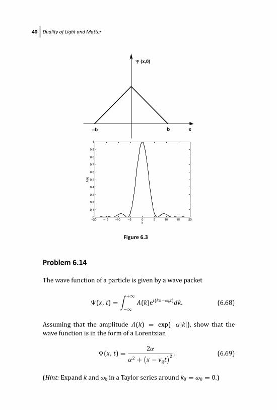
Figure 6.3 shows the wave packet �(x , 0) and the amplitude A(k)
for b = 1. The width of the wave packet is 2b, whereas the width of
the amplitude A(k) is 2π .
March 18, 2016 13:47 PSP Book - 9in x 6in Zbigniew-Ficek-tutsol
40 Duality of Light and Matter
x−b b
Ψ (x,0)
−20 −15 −10 −5 0 5 10 15 200
0.1
0.2
0.3
0.4
0.5
0.6
0.7
0.8
0.9
1
k
A(k
)
Figure 6.3
Problem 6.14
The wave function of a particle is given by a wave packet
�(x , t) =∫ +∞
−∞A(k)ei(kx−ωkt)dk. (6.68)
Assuming that the amplitude A(k) = exp(−α|k|), show that the
wave function is in the form of a Lorentzian
�(x , t) = 2α
α2 + (x − vgt
)2. (6.69)
(Hint: Expand k and ωk in a Taylor series around k0 = ω0 = 0.)
March 18, 2016 13:47 PSP Book - 9in x 6in Zbigniew-Ficek-tutsol
Duality of Light and Matter 41
Solution
Since A(k) = exp(−α|k|), the amplitude of the wave packet has the
explicit form
A(k) =⎧⎨⎩
eαk for k < 0,
e−αk for k ≥ 0.
(6.70)
Therefore, the wave function can be written as
�(x , t) =∫ +∞
−∞e−α|k|ei(kx−ωkt)dk
=∫ 0
−∞eαkei(kx−ωkt)dk +
∫ +∞
0
e−αkei(kx−ωkt)dk. (6.71)
Since ωk depends on k and the explicit dependence is unknown, we
may expand k and ωk in a Taylor series around k0 = ω0 = 0, i.e., we
can write
k ≈ k0 + β = β,
ωk ≈ ω0 + dωk
dkβ = vgβ, (6.72)
and obtain
�(x , t) =∫ 0
−∞eαβei(x−vgt)βdβ +
∫ +∞
0
e−αβei(x−vgt)βdβ . (6.73)
We can change the variable β to −β in the first integral and then
obtain
�(x , t) =∫ +∞
0
e−αβe−i(x−vgt)βdβ +∫ +∞
0
e−αβei(x−vgt)βdβ
=∫ +∞
0
e−αβ[e−i(x−vgt)β + ei(x−vgt)β
]dβ. (6.74)
Using Euler’s formula (e±i x = cos x ± i sin x) and performing the
integration, the above wave function simplifies to
�(x , t) = 2
∫ +∞
0
e−αβ cos[(x − vgt)β
]dβ
= 2e−αβ
α2 + (x − vgt)2
× {−α cos[(x − vgt)β
]+ (x − vgt) sin[(x − vgt)β
]}∣∣+∞0
= 2α
α2 + (x − vgt)2. (6.75)
March 18, 2016 13:47 PSP Book - 9in x 6in Zbigniew-Ficek-tutsol
42 Duality of Light and Matter
−20 −15 −10 −5 0 5 10 15 200
0.2
0.4
0.6
0.8
1
1.2
1.4
1.6
1.8
2
x
Ψ (
x,t)
t=0 t =x/vg
Figure 6.4
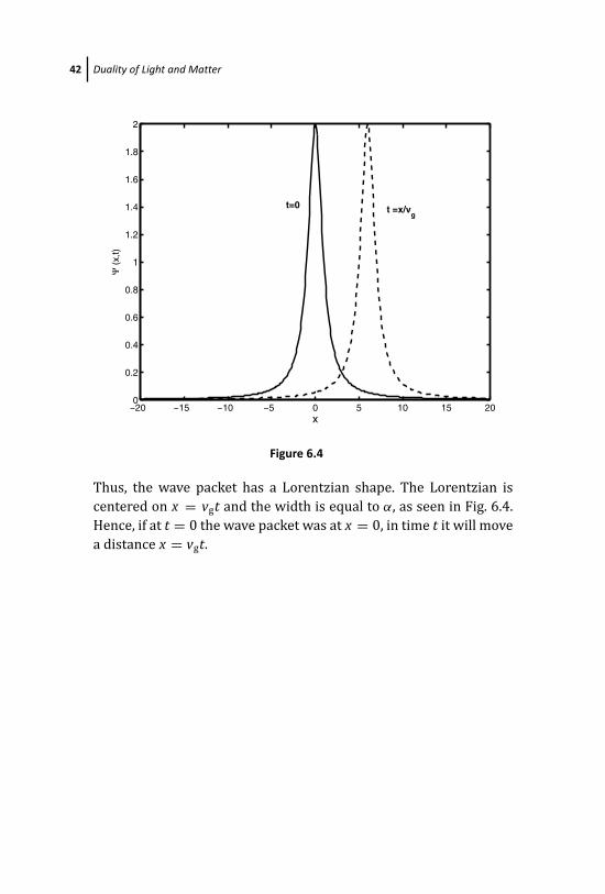
Thus, the wave packet has a Lorentzian shape. The Lorentzian is
centered on x = vgt and the width is equal to α, as seen in Fig. 6.4.
Hence, if at t = 0 the wave packet was at x = 0, in time t it will move
a distance x = vgt.
March 18, 2016 13:47 PSP Book - 9in x 6in Zbigniew-Ficek-tutsol
Chapter 7
Non-Relativistic Schrodinger Equation
Problem 7.1
Usually, we find the wave function by knowing the potential V (x).
Consider, however, an inverse problem where we know the wave
function and would like to determine the potential that leads to the
behavior described by the wave function.
Assume that a particle is confined within the region 0 ≤ x ≤ a,
and its wave function is
φ(x) = sin(πx
a
). (7.1)
Using the stationary Schrodinger equation, find the potential V (x)
confining the particle.
Solution
The Schrodinger equation involves the second-order derivative of
the wave function. Thus, finding the second-order derivatives of the
wave function
dφ(x)
dx= π
acos
(πxa
),
Problems and Solutions in Quantum PhysicsZbigniew FicekCopyright c© 2016 Pan Stanford Publishing Pte. Ltd.ISBN 978-981-4669-36-8 (Hardcover), 978-981-4669-37-5 (eBook)www.panstanford.com
March 18, 2016 13:47 PSP Book - 9in x 6in Zbigniew-Ficek-tutsol
44 Non-Relativistic Schrodinger Equation
d2φ(x)
dx2= −
(π
a
)2
sin(πx
a
), (7.2)
the stationary Schrodinger equation then takes the form
�2
2m
(π
a
)2
sin(πx
a
)+ V (x) sin
(πxa
)= E sin
(πxa
). (7.3)
We can write this expression as[�
2
2m
(π
a
)2
+ V (x) − E]
sin(πx
a
)= 0. (7.4)
This equation must be satisfied for all x within the region 0 ≤ x ≤ a,
which means that the expression in the squared brackets must be
zero, i.e.,
�2
2m
(π
a
)2
+ V (x) − E = 0. (7.5)
Note that the wave function is in the form of a sine function sin(kx),
which means that
k = π
a, (7.6)
so then
E = �2k2
2m= �
2π2
2ma2. (7.7)
Substituting this expression for E into Eq. (7.5), we easily find that
V (x) = 0. Thus, φ(x) is the wave function of a particle moving in the
potential V (x) = 0.
Problem 7.2
Another example of the inverse problem where we know the wave
function and would like to determine the potential that leads to the
behavior described by the wave function.
Consider the one-dimensional stationary wave function
φ(x) = A(
xx0
)n
e−x/x0 , (7.8)
where A, x0, and n are constants.
Using the stationary Schrodinger equation, find the potential
V (x) and the energy E for which this wave function is an
eigenfunction.
Assume that V (x) → 0 as x → ∞.
March 18, 2016 13:47 PSP Book - 9in x 6in Zbigniew-Ficek-tutsol
Non-Relativistic Schrodinger Equation 45
Solution
Consider a stationary one-dimensional Schrodinger equation(− �
2
2md2
dx2+ V (x)
)φ(x) = Eφ(x), (7.9)
which is the eigenvalue equation for the Hamiltonian of a particle of
mass m moving in the potential V (x).
Note that the equation involves the second-order derivative of
the wave function. Thus, we take derivatives of the wave function
dφ(x)
dx= A
nx0
(xx0
)n−1
e−x/x0 + A(
xx0
)n (−1
x0
)e−x/x0 , (7.10)
d2φ(x)
dx2= A
n(n − 1)
x20
(xx0
)n−2
e−x/x0
−2Anx2
0
(xx0
)n−1
e−x/x0 + A1
x20
(xx0
)n
e−x/x0
=[
n(n − 1)
x2− 2
nx x0
+ 1
x20
]φ(x). (7.11)
Substituting the above result into the Schrodinger equation, we find
that φ(x) is an eigenfunction with the eigenvalue E when
− �2
2m
[n(n − 1)
x2− 2
nx x0
+ 1
x20
]= E − V (x). (7.12)
As V (x) → 0 when x → ∞, we have
E = − �2
2mx20
, (7.13)
and hence
V (x) = �2
2m
[n(n − 1)
x2− 2n
x x0
]. (7.14)
A comment: The above potential is an example of an effective
potential for a hydrogen-like atom
V (x) = e2
r− l(l + 1)�2
2mr2, (7.15)
where the first term on the right-hand side is the Coulomb potential
and the second term is the so-called screening potential.
March 18, 2016 13:47 PSP Book - 9in x 6in Zbigniew-Ficek-tutsol
46 Non-Relativistic Schrodinger Equation
Problem 7.3
Consider the three-dimensional time-dependent Schrodinger equa-
tion of a particle of mass m moving with a potential V (�r , t):
i�∂�(�r , t)
∂t=(
− �2
2m∇2 + V (�r , t)
)�(�r , t). (7.16)
(a) Explain, what must be assumed about the form of the potential
energy to make the equation separable into a time-independent
Schrodinger equation and an equation for the time dependence
of the wave function.
(b) Using the condition stated in part (a), separate the time-
dependent Schrodinger equation into a time-independent
Schrodinger equation and an equation for the time-dependent
part of the wave function.
(c) Solve the equation for the time-dependent part of the wave
function and explain why the wave function of the separable
Schrodinger equation is a stationary state of the particle.
Solution (a)
The Hamiltonian of the particle involved in the Schrodinger equation
H (�r , t) = − �2
2m∇2 + V (�r , t), (7.17)
depends on the spatial variables through the kinetic and the
potential energies, and also on time but only through the potential
energy. If the potential energy is independent of time, then the
Hamiltonian depends solely on the spatial variables. In other words,
the Hamiltonian does not affect the time dependence of the wave
function of the particle. Therefore, the wave function �(�r , t) can be
written as a product of two parts, �(�r , t) = φ(�r) f (t), where φ(�r) is a
part of the wave function that depends solely on the spatial variables
and f (t) is a part that depends solely on time.
March 18, 2016 13:47 PSP Book - 9in x 6in Zbigniew-Ficek-tutsol
Non-Relativistic Schrodinger Equation 47
Solution (b)
If �(�r , t) = φ(�r) f (t), then the Schrodinger equation takes the form
i�φ(�r)∂ f (t)
∂t= f (t)
[− �
2
2m∇2 + V (�r)
]φ(�r), (7.18)
where we have used the fact that φ(�r) is a constant for the
differentiation over time and f (t) is a constant for the differentiation
over r . Equation (7.18) can be written as
i�1
f (t)
∂ f (t)
∂t= 1
φ(�r)
[− �
2
2m∇2 + V (�r)
]φ(�r), (7.19)
in which we see that both sides of the equation depend on different
(independent) variables. Thus, both sides must be equal to a
constant, say E :
i�1
f (t)
∂ f (t)
∂t= E ,
1
φ(�r)
[− �
2
2m∇2 + V (�r)
]φ(�r) = E . (7.20)
Thus, after the separation of the variables, we get two independent
ordinary differential equations
i�∂ f (t)
∂t= E f (t), (7.21)[
− �2
2m∇2 + V (�r)
]φ(�r) = Eφ(�r). (7.22)
Solution (c)
We can solve the time-dependent part, Eq. (7.21), using the method
of separate variables
d f (t)
f (t)= E
i�dt. (7.23)
Integrating both sides over time, we get
ln f (t) = −iE�
t, (7.24)
which gives
f (t) = f (0)e−i E�
t . (7.25)
March 18, 2016 13:47 PSP Book - 9in x 6in Zbigniew-Ficek-tutsol
48 Non-Relativistic Schrodinger Equation
The time-dependent part of the wave function varies in time as an
exponential function. Since the probability of finding the particle at
a point �r and at time t is given by the square of the absolute value of
the wave function, we have
| f (t)|2 = | f (0)|2. (7.26)
Clearly, the probability is independent of time. In other words, the
probability is constant in time. In physics, quantities that do not
change in time are called stationary in time. Thus, the wave function
of the separable Schrodinger equation is a stationary state of the
particle.
Problem 7.4
Consider the wave function
�(x , t) = (Aeikx + Be−ikx) eiωt . (7.27)
(a) Find the probability current corresponding to this wave
function.
(b) How would you interpret the physical meaning of the parame-
ters A and B?
Solution (a)
The probability current is defined by
�J = �
2im(�∗∇� − �∇�∗) . (7.28)
Since the wave function describes a particle moving in one
dimension, the x direction, the probability current for the one-
dimensional case simplifies to
�J = �
2im
(�∗ d�
dx− �
d�∗
dx
)i , (7.29)
where i is the unit vector in the x direction.
March 18, 2016 13:47 PSP Book - 9in x 6in Zbigniew-Ficek-tutsol
Non-Relativistic Schrodinger Equation 49
If we take the derivative
d�(x , t)
dx= ik
(Aeikx − Be−ikx) eiωt ,
d�∗(x , t)
dx= −ik
(A∗e−ikx − B∗eikx) e−iωt , (7.30)
we get for the probability current
�J = �km
[(A∗e−ikx + B∗eikx) (Aeikx − Be−ikx)
+ (Aeikx + Be−ikx) (A∗e−ikx − B∗eikx)] i
= �km
(|A|2 − |B|2)
i . (7.31)
Solution (b)
The probability current
�J = �km
(|A|2 − |B|2)
i (7.32)
is a superposition of two currents of particles of mass m moving
in opposite directions. Thus, it can be written as the sum of two
currents
�J = �J + + �J −, (7.33)
where
�J + = �km
|A|2 i (7.34)
is a current propagating to the right, in the +x direction, and
�J − = −�km
|B|2 i (7.35)
is a current propagating to the left, in the −x direction.
Hence, A can be interpreted as the amplitude of the probability
current propagating in the +x direction, and B can be interpreted as
the amplitude of the current propagating in the −x direction.

This page intentionally left blankThis page intentionally left blank
March 18, 2016 13:47 PSP Book - 9in x 6in Zbigniew-Ficek-tutsol
Chapter 8
Applications of Schrodinger Equation:Potential (Quantum) Wells
Problem 8.2
Solve the stationary Schrodinger equation for a particle not bounded
by any potential and show that its total energy E is not quantized.
Solution
When V (x) = 0, i.e., when the particle is not bounded by any
potential we can rearrange the Schrodinger equation to the form
d2φ(x)
dx2= −2m
�2Eφ(x) = −k2φ(x), (8.1)
which is a second-order differential equation with a constant
positive coefficient k2 = 2mE/�2.
The solution to Eq. (8.1) is either a sine or cosine function, which
in general can be written in terms of complex exponentials, such as
φ(x) = Aeikx + Be−ikx , (8.2)
where A and B are constants. Since there are no potentials that could
bound the particle, the solution (8.2) is valid for all x and there are
Problems and Solutions in Quantum PhysicsZbigniew FicekCopyright c© 2016 Pan Stanford Publishing Pte. Ltd.ISBN 978-981-4669-36-8 (Hardcover), 978-981-4669-37-5 (eBook)www.panstanford.com
March 18, 2016 13:47 PSP Book - 9in x 6in Zbigniew-Ficek-tutsol
52 Applications of Schrodinger Equation
no restrictions on k. If there are no restrictions on k, it means that
there are no restrictions on E = �2k2/2m. Thus, for the particle
moving in an unbounded area where the potential V (x) = 0, there
are no restrictions on k, which means that there are no restrictions
on the energy E of the particle. Hence, E can have any value ranging
from zero to +∞ (continuous spectrum).
Problem 8.3
Solve the Schrodinger equation with appropriate boundary condi-
tions for an infinite square well with the width of the well a centered
at a/2, i.e.,
V (x) = 0 for 0 ≤ x ≤ a ,
V (x) = ∞ for x < 0 and x > a. (8.3)
Check that the allowed energies are consistent with those derived
in the chapter for an infinite well of width a centered at the origin.
Confirm that the wave function φn(x) can be obtained from those
found in the chapter if one uses the substitution x → x + a/2.
Solution
In the regions x < 0 and x > a, the potential is infinite. Therefore,
in those regions, the wave function is equal to zero. Since the wave
function must be continuous at x = 0 and x = a, we have φ(x) = 0
at these points.
In the region 0 ≤ x ≤ a, the wave function is of the form
φ(x) = Aeikx + Be−ikx . (8.4)
Thus, at x = 0, the wave function φ(x) = 0 when
A + B = 0. (8.5)
At x = a, the wave function φ(x) = 0 when
Aeika + Be−ika = 0. (8.6)
From Eq. (8.5), we find
B = −A , (8.7)
March 18, 2016 13:47 PSP Book - 9in x 6in Zbigniew-Ficek-tutsol
Applications of Schrodinger Equation 53
whereas from Eq. (8.6), we find
B = −Ae2ika . (8.8)
We have obtained two different solutions for the coefficient B . We
cannot accept these two different solutions, as one of the conditions
imposed on the wave function says that the wave function must be
a single-value function. Therefore, we have to find a condition under
which the two solutions (8.7) and (8.8) are equal. It is easy to see
that the two solutions for B will be equal if
e−2ika = 1, (8.9)
which will be satisfied when
e−2ika = cos(2ka) − i sin(2ka) = 1, (8.10)
or when
sin(2ka) = 0 and cos(2ka) = 1, (8.11)
i.e., when
k = nπ
a, with n = 0, 1, 2, . . . . (8.12)
Since k2 = 2mE/�2, we get for the energy
En = �2
2mk2 = n2 π2
�2
2ma2. (8.13)
Comparing Eq. (8.13) with Eq. (8.21) of the textbook, we see that
the expressions for the energy of the particle inside the well are the
same, i.e., the energy, independent of the choice of the coordinates.
Substituting either Eq. (8.7) or (8.8) into the general solution to
the wave function, Eq. (8.4), we find the wave function of the particle
inside the well
φn(x) = A sin(nπx
a
), with n = 1, 2, 3, . . . , (8.14)
where the coefficient A is found from the normalization condition∫ +∞
−∞dx|φn(x)|2 = |A|2
∫ +∞
−∞dx sin2
(nπxa
)= 1. (8.15)
Performing integration with the wave function φn(x) given by
Eq. (8.14), we find A = √2/a.
Comparing the solution to the wave function, Eq. (8.14), with the
solution (8.22) of the textbook, we see that the wave function (8.14)
can be obtained from that of the textbook by simply substituting in
Eq. (8.22), x → x + a/2.
March 18, 2016 13:47 PSP Book - 9in x 6in Zbigniew-Ficek-tutsol
54 Applications of Schrodinger Equation
Problem 8.4
Show that as n → ∞, the probability of finding a particle between xand x + x inside an infinite potential well is independent of x ,
which is the classical expectation. This result is an example of the
correspondence principle that quantum theory should give the same
results as classical physics in the limit of large quantum numbers.
Solution
The probability of finding a particle between x and x + x is given
by
P = |φn(x)|2x . (8.16)
For a particle inside an infinite potential well, the wave function is
given by Eq. (8.14), so the probability is
P = 2
asin2
(nπxa
)x = 1
a
[1 − cos
(2nπx
a
)]x . (8.17)
When n → ∞, cos (2nπx/a) → 0, and then
P → 1
ax . (8.18)
Clearly, the probability is independent of x . In other words, the
probability is the same for any region x inside the well.
Problem 8.5
As we have already learned, the exclusion of E = 0 as a possible
value for the energy of the particle and the limitation of E to
a discrete set of definite values are examples of quantum effects
that have no counterpart in classical physics, where all energies,
including zero, are presumed possible.
Why we do not observe these quantum effects in everyday life?
March 18, 2016 13:47 PSP Book - 9in x 6in Zbigniew-Ficek-tutsol
Applications of Schrodinger Equation 55
Solution
We may answer this question by looking at the expression for the
energy of a particle inside a potential well given by
En = n2 π2�
2
2ma2, (8.19)
where m is the mass of the particle and a is the width (size) of the
well.
The energy difference between two neighbouring states, say nand n − 1, is
En − En−1 = (2n − 1)π2
�2
2ma2. (8.20)
In order to distinguish the energy states, the difference between
the energies of two neighbouring states should be large. It should
be larger than the uncertainty of the energy of the particle. We see
from the above expression that the energy difference is inversely
proportional to the mass of the particle and the size of the well.
These two parameters should be very small to have the energy
difference large. Such small values can be achieved with small
particles, such as electrons, and with structures of nano-sizes. Such
objects are called microscopic objects. In everyday life, we deal with
visible (macroscopic) objects, whose masses and sizes are very large
compared to the mass and size of the electron. For a macroscopic
object bounded in a well, the difference between the energies of the
energy states is negligibly small so that a continuous rather than a
discrete energy spectrum is observed.
Problem 8.6
What length scale is required to observe discrete (quantized)
energies of an electron confined in an infinite potential well?
Calculate the width of the potential well in which a low-energy
electron, being in the energy state n = 2, emits a visible light of
wavelength λ = 700 nm (red) when making a transition to its
ground state n = 1. Compare the length scale (width) to the size
of an atom ∼ 0.1 nm.
March 18, 2016 13:47 PSP Book - 9in x 6in Zbigniew-Ficek-tutsol
56 Applications of Schrodinger Equation
Solution
An electron inside an infinite potential well can have energies
En = n2 π2�
2
2ma2, (8.21)
where m is the mass of the electron and a is the width of the well.
The energy difference between n = 2 and n = 1 is equal to
E2 − E1 = �ω, (8.22)
where ω is the angular frequency of light emitted. Since ω = 2πc/λ,
where λ is the wavelength of the emitted light, we get
E2 − E1 = 3π2�
2
2ma2= �
2πcλ
, (8.23)
from which we find
a =(
3π�λ
4mc
) 12
. (8.24)
Substituting the values of the parameters
m = 9.11 × 10⁻³¹ kg, c = 3 × 10⁸ m/s,
� = 1.055 × 10⁻³⁴ J.s, λ = 700 nm = 700 × 10−9 m, (8.25)
we find
a = 0.8 × 10⁻⁹ m = 0.8 nm. (8.26)
The size of the well is about eight times the size of an atom.
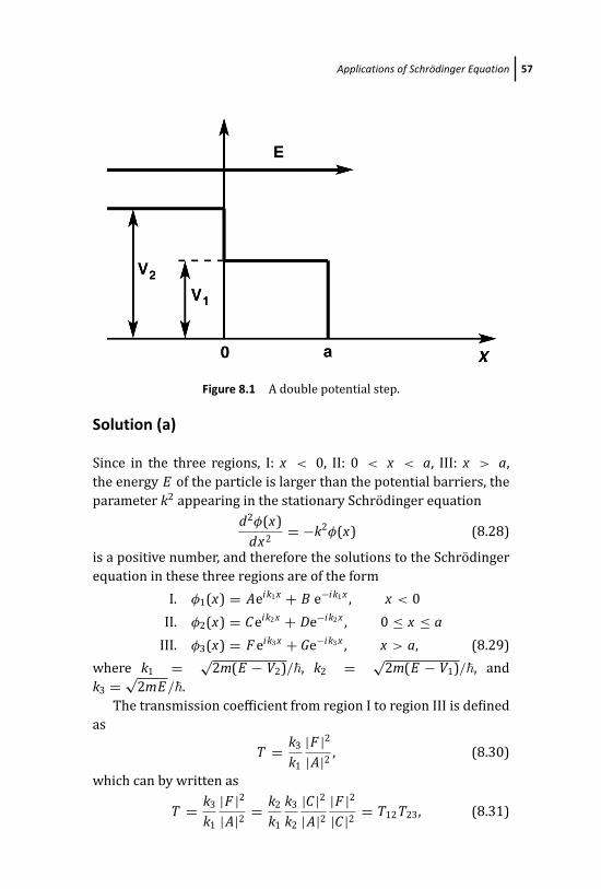
Problem 8.7
Particles of mass m and energy E moving in one dimension from −xto +x encounter a double potential step, as shown in Fig. 8.1, where
V1 = π2�
2
8ma2, E = 2V1, V1 < V2 < E . (8.27)
(a) Find the transmission coefficient T .
(b) Find the value of V2 at which T is maximum.
March 18, 2016 13:47 PSP Book - 9in x 6in Zbigniew-Ficek-tutsol
Applications of Schrodinger Equation 57
Figure 8.1 A double potential step.
Solution (a)
Since in the three regions, I: x < 0, II: 0 < x < a, III: x > a,
the energy E of the particle is larger than the potential barriers, the
parameter k2 appearing in the stationary Schrodinger equation
d2φ(x)
dx2= −k2φ(x) (8.28)
is a positive number, and therefore the solutions to the Schrodinger
equation in these three regions are of the form
I. φ1(x) = Aeik1 x + B e−ik1 x , x < 0
II. φ2(x) = C eik2 x + De−ik2 x , 0 ≤ x ≤ a
III. φ3(x) = F eik3 x + Ge−ik3 x , x > a, (8.29)
where k1 = √2m(E − V2)/�, k2 = √
2m(E − V1)/�, and
k3 = √2mE/�.
The transmission coefficient from region I to region III is defined
as
T = k3
k1
|F |2
|A|2, (8.30)
which can by written as
T = k3
k1
|F |2
|A|2= k2
k1
k3
k2
|C |2
|A|2
|F |2
|C |2= T12T23, (8.31)
March 18, 2016 13:47 PSP Book - 9in x 6in Zbigniew-Ficek-tutsol
58 Applications of Schrodinger Equation
where
T12 = k2
k1
|C |2
|A|2(8.32)
is the transmission coefficient from region I to region II, and
T23 = k3
k2
|F |2
|C |2(8.33)
is the transmission coefficient from region II to region III.
We find the ratios |C |2
|A|2 and |F |2
|C |2 from the continuity conditions for
the wave function and the first-order derivative at x = 0 and x = a.
Since we expect that the particle transmitted to region III will move
to the right (to the positive x), with no particle traveling to the left,
we put G = 0 in the wave function in region III.
The continuity conditions for the wave function and the first-
order derivative at x = 0 are
A + B = C + D, (8.34)
ik1 A − ik1 B = ik2C − ik2 D. (8.35)
The continuity conditions at x = a are
C eik2a + De−ik2a = F eik3a , (8.36)
ik2C eik2a − ik2 De−ik2a = ik3 F eik3a . (8.37)
The set of coupled equations (8.34) and (8.35) can be written
as
A + B = C + D, (8.38)
A − B = α(C − D), (8.39)
while Eqs. (8.36) and (8.37) can be written as
C eik2a + De−ik2a = F eik3a , (8.40)
C eik2a − De−ik2a = β F eik3a , (8.41)
where α = k2/k1 and β = k3/k2.
First, we will find from Eqs. (8.40) and (8.41) the constants C and
D in terms of F , which will give us the required ratio |F |2/|C |2.
By adding Eqs. (8.40) and (8.41), we obtain
2C eik2a = (1 + β)F eik3a , (8.42)
March 18, 2016 13:47 PSP Book - 9in x 6in Zbigniew-Ficek-tutsol
Applications of Schrodinger Equation 59
from which, we find
C = 1
2(1 + β)F ei(k3−k2)a . (8.43)
Similarly, by subtracting Eqs. (8.40) and (8.41), we obtain
2De−ik2a = (1 − β)F eik3a , (8.44)
from which, we find
D = 1
2(1 − β)F ei(k3+k2)a . (8.45)
Thus, we find from Eq. (8.43) that
FC
= 2
(1 + β)e−i(k3−k2)a , (8.46)
from which we obtain
|F |2
|C |2= 4
(1 + β)2. (8.47)
Now, we will find the ratio |C |2
|A|2 . By adding Eqs. (8.38) and (8.39), we
obtain
2A = (1 + α)C + (1 − α)D, (8.48)
and substituting for D from Eq. (8.45), we find
2A = (1 + α)C + 1
2(1 − α)(1 − β)F ei(k3+k2)a
= (1 + α)C + 1
2(1 − α)(1 − β)ei(k3+k2)a 2C
(1 + β)e−i(k3−k2)a
=[
(1 + α) + (1 − α)(1 − β)
(1 + β)e2ik2a
]C . (8.49)
Thus,
CA
= 2(1 + β)[(1 + α)(1 + β) + (1 − α)(1 − β)e2ik2a
] . (8.50)
However,
2k2a = 2
√2m�2
(E − V1)a = 2
√2m�2
V1a = 2
√2m�2
π2�2
8ma2a = π.
(8.51)
Hence
e2ik2a = eiπ = −1, (8.52)
March 18, 2016 13:47 PSP Book - 9in x 6in Zbigniew-Ficek-tutsol
60 Applications of Schrodinger Equation
and thenCA
= 2(1 + β)[(1 + α)(1 + β) + (1 − α)(1 − β)e2ik2a
]= 2(1 + β)
[(1 + α)(1 + β) − (1 − α)(1 − β)]
= (1 + β)
(α + β). (8.53)
Thus
|C |2
|A|2= (1 + β)2
(α + β)2. (8.54)
With the solutions (8.47) and (8.54), we find the transmission
coefficients
T12 = k2
k1
|C |2
|A|2= α
(1 + β)2
(α + β)2,
T23 = k3
k2
|F |2
|C |2= β
4
(1 + β)2, (8.55)
which lead to the total transmission coefficient
T = T12T23 = 4αβ
(α + β)2. (8.56)
Solution (b)
It is easy to see from the above equation that the transmission
coefficient is maximum, T = 1, when α = β , i.e., when
k2
k1
= k3
k2
, (8.57)
from which we find that T = 1 when
k22 = k1k3 . (8.58)
Substituting the explicit forms of k1, k2, and k3, we obtain
2m�2
(E − V1) = 2m�2
√E (E − V2) (8.59)
from which, we get
(E − V1) =√
E (E − V2). (8.60)
Since E = 2V1, we find from the above equation
V1 =√
2V1 (2V1 − V2) ⇒ V2 = 3
2V1. (8.61)
March 18, 2016 13:47 PSP Book - 9in x 6in Zbigniew-Ficek-tutsol
Applications of Schrodinger Equation 61
Problem 8.8
Show that the particle probability current density �J is zero in region
I, and deduce that R = 1, T = 0. This is the case of total reflection;
the particle coming toward the barrier will eventually be found
moving back. “Eventually”, because the reversal of direction is not
sudden. Quantum barriers are “spongy” in the sense the quantum
particle may penetrate them in a way that classical particles may not.
Solution
The probability current is defined as
�J = �
2im
(φ∗ dφ
dx− φ
dφ∗
dx
). (8.62)
In region I, the wave function of the particles is
φ1(x) = C ek1 x . (8.63)
Hence
dφ1
dx= k1C ek1 x . (8.64)
and then
φ∗1
dφ1
dx= k1|C |2e2k1 x . (8.65)
By taking the complex conjugate of the above equation, we obtain
φ1
dφ∗1
dx= k1|C |2e2k1 x . (8.66)
Therefore, we see that
φ∗1
dφ1
dx− φ1
dφ∗1
dx= 0. (8.67)
Thus
J 1 = �
2im
(φ∗
1
dφ1
dx− φ1
dφ∗1
dx
)= 0, (8.68)
i.e., in region I, the probability current is zero.
Consider now the wave function of the particle in region II
φ2(x) = Aeik2 x + Be−ik2 x . (8.69)
March 18, 2016 13:47 PSP Book - 9in x 6in Zbigniew-Ficek-tutsol
62 Applications of Schrodinger Equation
The first term on the right-hand side of this equation describes
particles moving to the right, away from the barrier between regions
I and II, whereas the second term describes particles moving to the
left, toward the barrier between I and II. Therefore, the amplitude Bcan be treated as an amplitude of particles incident on the barrier,
while A can be treated as an amplitude of particles reflected from
the barrier. Thus, we may introduce a reflection coefficient
R = |A|2
|B|2. (8.70)
Using the expression for the relation between A and B , Eq. (8.97) of
the textbook
A = (iβ + 1)
(iβ − 1)Beiak2 , (8.71)
we readily find that
R = |A|2
|B|2= |(iβ + 1)|2
|(iβ − 1)|2= (iβ + 1)(−iβ + 1)
(iβ − 1)(−iβ − 1)
= (iβ + 1)(iβ − 1)
(iβ − 1)(iβ + 1)= 1. (8.72)
The reflection coefficient R = 1 even if the particles can penetrate
the barrier.
Problem 8.9
Recall the case of E > V0, discussed briefly in Section 8.3.1 of the
textbook.
(a) Evaluate the transmission coefficient from region I to region III.
(b) Under which condition, the transmission coefficient becomes
unity (T = 1)?
March 18, 2016 13:47 PSP Book - 9in x 6in Zbigniew-Ficek-tutsol
Applications of Schrodinger Equation 63
Solution (a)
The general solution to the Schrodinger equation for the wave
function of the particle with energy E > V0 is of the form
I. φ1(x) = C eik1 x + De−ik1 x , x < −a2
II. φ2(x) = Aeik2 x + Be−ik2 x , −a2
≤ x ≤ a2
III. φ3(x) = F eik1 x , x >a2
. (8.73)
The transmission coefficient from region I to region III is given by
the ratio T = |F |2/|C |2. Thus, we will try to find the coefficient Fin terms of C using the properties of the wave function: φ(x) and
the first-order derivative dφ(x)/dx must be finite and continuous
everywhere, in particular, at the boundaries x = −a/2 and x = a/2.
The first-order derivatives of the wave function in different
regions are
I.dφ1
dx= ik1C eik1 x − ik1 De−ik1 x ,
II.dφ2
dx= ik2 Aeik2 x − ik2 Be−ik2 x ,
III.dφ3
dx= ik1 F eik1 x . (8.74)
From the continuity of the wave function and the first derivatives at
x = −a/2, we get
C e− 12
iak1 + De12
iak1 = Ae−i 12
ak2 + Bei 12
ak2 ,
ik1C e− 12
iak1 − ik1 De12
iak1 = ik2 Ae−i 12
ak2 − ik2 Bei 12
ak2 , (8.75)
which can be written as
C e− 12
iak1 + De12
iak1 = Ae−i 12
ak2 + Bei 12
ak2 ,
C e− 12
iak1 − De12
iak1 = β Ae−i 12
ak2 − β Bei 12
ak2 , (8.76)
where β = k2/k1.
By adding the two equations in (8.76), we get C in terms of A and
B:
2C e− 12
iak1 = (β + 1)Ae−i 12
ak2 + (1 − β)Bei 12
ak2 , (8.77)
March 18, 2016 13:47 PSP Book - 9in x 6in Zbigniew-Ficek-tutsol
64 Applications of Schrodinger Equation
From the continuity of the wave function and the first derivatives at
x = a/2, we get
F e12
iak1 = Aei 12
ak2 + Be−i 12
ak2 ,
ik1 F e12
iak1 = ik2 Aei 12
ak2 − ik2 Be−i 12
ak2 , (8.78)
which can be written as
F e12
iak1 = Aei 12
ak2 + Be−i 12
ak2 ,
F e12
iak1 = β Aei 12
ak2 − β Be−i 12
ak2 . (8.79)
Since the left-hand sides of the above equations are equal, we
get
Aei 12
ak2 + Be−i 12
ak2 = β Aei 12
ak2 − β Be−i 12
ak2 , (8.80)
from which we find B in terms of A as
B = (β − 1)
(β + 1)Aeiak2 . (8.81)
Substituting Eq. (8.81) in either of the expressions in (8.79), we get
F in terms of A:
F = Auei 12
a(k2−k1), (8.82)
where u = 2β/(β + 1).
Substituting Eq. (8.81) into Eq. (8.77), we get C in terms of A:
C = 1
2Ae
12
ia(k1+k2)
[(β + 1)e−iak2 − (1 − β)2
(β + 1)eiak2
]. (8.83)
For the transmission coefficient, we need |F |2 and |C |2. From
Eq. (8.82), we have
|F |2 = |A|2u2, (8.84)
and from Eq. (8.83), we have
|C |2 = 1
4|A|2
{4u2 + 2(β − 1)2 [1 − cos(2ak2)]
}. (8.85)
Thus, the transmission coefficient is of the form
T = |F |2
|C |2= 4u2
4u2 + 2(β − 1)2 [1 − cos(2ak2)]. (8.86)
Note that in general T < 1, showing that even when E > V0, not all
particles can be transmitted to region III, a part of the particles can
be reflected back to region I.
March 18, 2016 13:47 PSP Book - 9in x 6in Zbigniew-Ficek-tutsol
Applications of Schrodinger Equation 65
Solution (b)
Lets look more closely at the expression for the transmission
coefficient derived in part (a):
T = 4u2
4u2 + 2(β − 1)2 [1 − cos(2ak2)]. (8.87)
It is easily seen that there are two different conditions for T = 1. The
first one is a trivial, β = 1 or equivalently k1 = k2, and corresponds
to the situation of V0 = 0, i.e., there is no potential barrier. The
second condition is more interesting and corresponds to
cos(2ak2) = 1, (8.88)
which happens when
2ak2 = 2πn, n = 0, 1, 2, . . . (8.89)
or when the energy of the particle satisfies the conditions
E = n2 π2�
2
2ma2. (8.90)
Thus, for some discrete energies E > V0, the transmission coefficient
from region I to region III equals T = 1, independent of the value of
V0.
Problem 8.10
A rectangular potential well is bounded by a wall of infinite high on
one side and a wall of high V0 on the other, as shown in Figure 8.2.
The well has a width a, and a particle located inside the well has
energy E < V0.
(a) Find the wave function of the particle inside the well.
(b) Show that the energy of the particle is quantized.
(c) Discuss the dependence of the number of energy levels inside
the well on V0.
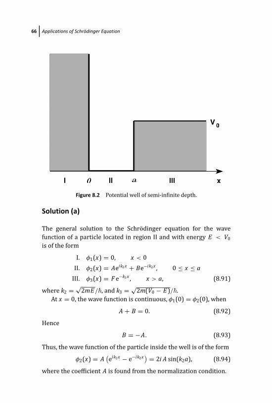
March 18, 2016 13:47 PSP Book - 9in x 6in Zbigniew-Ficek-tutsol
66 Applications of Schrodinger Equation
Figure 8.2 Potential well of semi-infinite depth.
Solution (a)
The general solution to the Schrodinger equation for the wave
function of a particle located in region II and with energy E < V0
is of the form
I. φ1(x) = 0, x < 0
II. φ2(x) = Aeik2 x + Be−ik2 x , 0 ≤ x ≤ a
III. φ3(x) = F e−k3 x , x > a, (8.91)
where k2 = √2mE/�, and k3 = √
2m(V0 − E )/�.
At x = 0, the wave function is continuous, φ1(0) = φ2(0), when
A + B = 0. (8.92)
Hence
B = −A . (8.93)
Thus, the wave function of the particle inside the well is of the form
φ2(x) = A(
eik2 x − e−ik2 x) = 2i A sin(k2a), (8.94)
where the coefficient A is found from the normalization condition.
March 18, 2016 13:47 PSP Book - 9in x 6in Zbigniew-Ficek-tutsol
Applications of Schrodinger Equation 67
Solution (b)
Consider the continuity conditions for the wave function and the
first-order derivatives at x = a:
φ2(a) = φ3(a),
dφ2(x)
dx
∣∣∣∣x=a
= dφ3(x)
dx
∣∣∣∣x=a
. (8.95)
The above continuity conditions lead to two equations for F :
F e−k3a = Aeik2a + Be−ik2a ,
−k3 F e−k3a = ik2 Aeik2a − ik2 Be−ik2a , (8.96)
which, after substituting B = −A, take the form
F e−k3a = Aeik2a − Ae−ik2a ,
F e−k3a = −iβ(
Aeik2a + Ae−ik2a) , (8.97)
where β = k2/k3.
Since eik2a − e−ik2a = 2i sin(k2a) and eik2a + e−ik2a = 2 cos(k2a),
the above equations can be simplified to
F e−k3a = 2i A sin(k2a),
F e−k3a = −2iβ A cos(k2a). (8.98)
Thus, we have two different solutions to F . However, we cannot
accept both the solutions as it would mean that there are two
different probabilities of finding the particle at a point x inside
region III. Therefore, we have to find under which circumstances
these two solutions are equal.
It is easily seen from Eq. (8.98) that the two solutions to F will be
equal when
sin(k2a) = −β cos(k2a), (8.99)
which can be written as
tan(k2a) = −β = −k2
k3
. (8.100)
Introduce a notation
ak2 =√
2ma2 E�2
= ε,
ak3 =√
2ma2(V0 − E )
�2=√
2ma2V0
�2− 2ma2 E
�2=√
η2 − ε2,
(8.101)
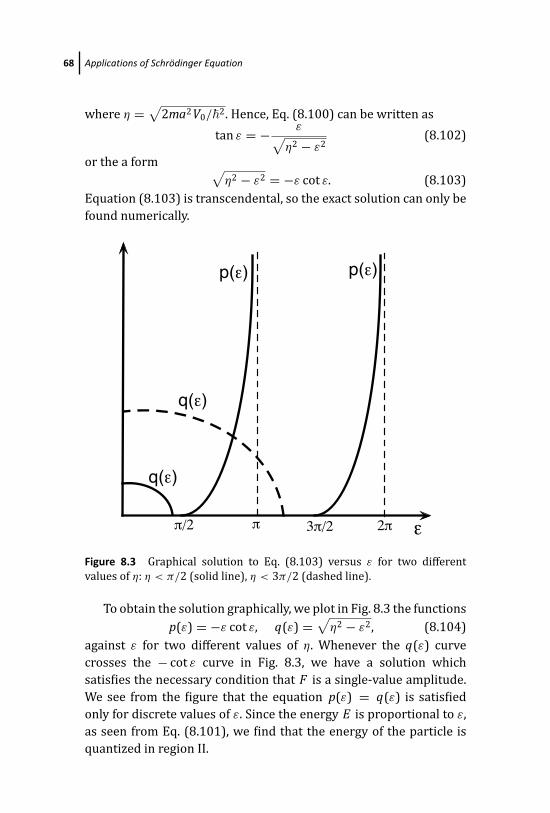
March 18, 2016 13:47 PSP Book - 9in x 6in Zbigniew-Ficek-tutsol
68 Applications of Schrodinger Equation
where η =√
2ma2V0/�2. Hence, Eq. (8.100) can be written as
tan ε = − ε√η2 − ε2
(8.102)
or the a form √η2 − ε2 = −ε cot ε. (8.103)
Equation (8.103) is transcendental, so the exact solution can only be
found numerically.
ε
p(ε) p(ε)
q(ε)
q(ε)
π/2 π 2π3π/2
Figure 8.3 Graphical solution to Eq. (8.103) versus ε for two different
values of η: η < π/2 (solid line), η < 3π/2 (dashed line).
To obtain the solution graphically, we plot in Fig. 8.3 the functions
p(ε) = −ε cot ε, q(ε) =√
η2 − ε2, (8.104)
against ε for two different values of η. Whenever the q(ε) curve
crosses the − cot ε curve in Fig. 8.3, we have a solution which
satisfies the necessary condition that F is a single-value amplitude.
We see from the figure that the equation p(ε) = q(ε) is satisfied
only for discrete values of ε. Since the energy E is proportional to ε,
as seen from Eq. (8.101), we find that the energy of the particle is
quantized in region II.
March 18, 2016 13:47 PSP Book - 9in x 6in Zbigniew-Ficek-tutsol
Applications of Schrodinger Equation 69
Solution (c)
It is easily seen from Fig. 8.3 that the number of crossing points of
q(ε) with p(ε) depends on the value of η. Note that the number of
crossings corresponds to a number of energy states fitted into the
well, region II. Thus, there is no crossing point when η < π/2. When
η < 3π/2 there is one crossing point, for η < 5π/2 there are two
crossing points, and so on.
It is interesting to note that there is a possibility of no energy
state allowed inside the well. Since, η =√
2ma2V0/�2, we see that
for
V0 <π2
�2
8ma2, (8.105)
there is no energy state allowed inside the well.
Problem 8.15
Particles of mass m and energy E < V0 moving in one dimension
from −x to +x encounter a non-symmetric barrier, as shown in
Fig. 8.4.
(a) Find the transmission coefficient T .
(b) Show that in the limit of a → 0, the transmission coefficient
reduces to that of the step potential.
(c) Does the transmission coefficient depend on the direction of
propagation of the particles?
Solution (a)
Since in regions I: x < −a and III: x > a, the energy E of the particle
is larger than the potential barriers, the parameter k2 appearing
in the stationary Schrodinger equation is a positive number, and
therefore the solutions to the Schrodinger equation in regions I and
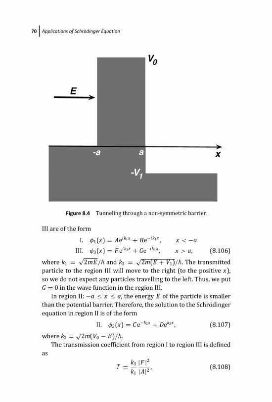
March 18, 2016 13:47 PSP Book - 9in x 6in Zbigniew-Ficek-tutsol
70 Applications of Schrodinger Equation
x
V0
E
-a
-V1
a
Figure 8.4 Tunneling through a non-symmetric barrier.
III are of the form
I. φ1(x) = Aeik1 x + Be−ik1 x , x < −a
III. φ3(x) = F eik3 x + Ge−ik3 x , x > a, (8.106)
where k1 = √2mE/� and k3 = √
2m(E + V1)/�. The transmitted
particle to the region III will move to the right (to the positive x),
so we do not expect any particles travelling to the left. Thus, we put
G = 0 in the wave function in the region III.
In region II: −a ≤ x ≤ a, the energy E of the particle is smaller
than the potential barrier. Therefore, the solution to the Schrodinger
equation in region II is of the form
II. φ2(x) = C e−k2 x + Dek2 x , (8.107)
where k2 = √2m(V0 − E )/�.
The transmission coefficient from region I to region III is defined
as
T = k3
k1
|F |2
|A|2, (8.108)
March 18, 2016 13:47 PSP Book - 9in x 6in Zbigniew-Ficek-tutsol
Applications of Schrodinger Equation 71
where the ratio |F |2/|A|2 is found from the continuity conditions
for the wave function and its first-order derivatives at x = −a and
x = a.
The continuity conditions at x = −a are
Ae−ik1a + Beik2a = C ek2a + De−k2a ,
ik1 Ae−ik1a − ik1 Beik1a = −k2C ek2a + k2 De−k2a . (8.109)
The above set of coupled equations, can be written as
Ae−ik1a + Beik2a = C ek2a + De−k2a , (8.110)
Ae−ik1a − Beik1a = iβC ek2a − iβ De−k2a . (8.111)
where β = k2/k1.
The continuity conditions at x = a are
C e−k2a + Dek2a = F eik3a ,
−k2C e−k2a + k2 Dek2a = ik3 F eik3a , (8.112)
which we can write as
C e−k2a + Dek2a = F eik3a , (8.113)
−C e−k2a + Dek2a = iγ F eik3a , (8.114)
where γ = k3/k2.
By adding Eqs. (8.110) and (8.111), we obtain
2Ae−ik1a = uC ek2a + u∗ De−k2a , (8.115)
where u = 1 + iβ and u∗ = 1 − iβ .
By adding and subtracting Eqs. (8.113) and (8.114), we find the
coefficients D and C in terms of F :
2Dek2a = wF eik3a , (8.116)
2C e−k2a = w∗ F eik3a , (8.117)
where w = 1 + iγ and w∗ = 1 − iγ .
Substituting Eqs. (8.116) and (8.117) into Eq. (8.115), we obtain
A in terms of F :
4Ae−ik1a = ue2k2aw∗ F eik3a + u∗e−2k2awF eik3a , (8.118)
from which we find
4Ae−i(k1+k3)a = F[uw∗e2k2a + u∗we−2k2a] . (8.119)
March 18, 2016 13:47 PSP Book - 9in x 6in Zbigniew-Ficek-tutsol
72 Applications of Schrodinger Equation
Thus|F |2
|A|2= 16
|uw∗e2k2a + u∗we−2k2a|2. (8.120)
Let us simplify the denominator on the right-hand side of the above
equation. It can be written as
|uw∗ e2k2a + u∗we−2k2a|2
= (uw∗e2k2a + u∗we−2k2a)(u∗we2k2a + uw∗e−2k2a)
= |u|2|w|2e4k2a + (u2w∗2 + u∗2w2) + |u|2|w|2e−4k2a
= |u|2|w|2(e4k2a + e−4k2a) + (u2w∗2 + u∗2w2)
= 2|u|2|w|2 cosh(4k2a) + (uw∗)2 + (u∗w)2. (8.121)
Since cosh(4k2a) = 1 + 2 sinh2(2k2a), we obtain
|F |2
|A|2= 16
(uw∗ + u∗w)2 + 4|u|2|w|2 sinh2(2k2a), (8.122)
and then the transmission coefficient can be written as
T = k3
k1
|F |2
|A|2= P
1 + Q sinh2(2k2a), (8.123)
where
P = k3
k1
16
(uw∗ + u∗w)2, (8.124)
Q = 4|u|2|w|2
(uw∗ + u∗w)2. (8.125)
In terms of the constants k1, k2, and k3, the coefficients P and Q are
P = k3
k1
16
(uw∗ + u∗w)2= k3
k1
16
4(1 + βγ )2= 4k3k1
(k1 + k3)2. (8.126)
and
Q = 4|u|2|w|2
(uw∗ + u∗w)2= 4(1 + β2)(1 + γ 2)
4(1 + βγ )2= (k1 + k2)2(k2 + k3)2
k22(k1 + k3)2
.
(8.127)
Solution (b)
In the limit of a → 0, the function sinh2(2k2a) → 0, and then the
transmission coefficient reduces to T = P , i.e.,
T = 4k3k1
(k1 + k3)2. (8.128)
This is precisely the result obtained for the step potential. For details
see Section 8.2 of the textbook Eq. (8.75), page 126.
March 18, 2016 13:47 PSP Book - 9in x 6in Zbigniew-Ficek-tutsol
Applications of Schrodinger Equation 73
Solution (c)
No, in terms of the constants k, the change in the direction of
propagation is equivalent to exchange k3 ↔ k1. We see from the
above that in this case, the coefficients P and Q remain the same.
This is an important result. Even though the barrier and energy
structure do not appear symmetrical, the barrier is a linear,
passive structure. Therefore, the transmission should be the same
regardless of the direction from which one approaches the barrier.

This page intentionally left blankThis page intentionally left blank
March 18, 2016 13:47 PSP Book - 9in x 6in Zbigniew-Ficek-tutsol
Chapter 9
Multidimensional Quantum Wells
Problem 9.1
This problem illustrates why the tunneling (flow) of an electron
between different quantum dots is possible only for specific
(discrete) energies of the electron.
Consider a simplified situation, a one-dimensional system of
quantum wells, as shown in Fig. 9.1. The well represents a quantum
dot. Show, using the method we learned in the previous chapter on
applications of the Schrodinger equation, that an electron of energy
E < V0 and being in region I can tunnel through the quantum well
(region II) to region III only if E is equal to the energy of one of the
discrete energy levels inside the well.
Solution
In fact, we can distinguish here five different regions for the wave
functions. The general solution to the Schrodinger equation for the
wave function of a particle in region I traveling to the right and with
Problems and Solutions in Quantum PhysicsZbigniew FicekCopyright c© 2016 Pan Stanford Publishing Pte. Ltd.ISBN 978-981-4669-36-8 (Hardcover), 978-981-4669-37-5 (eBook)www.panstanford.com
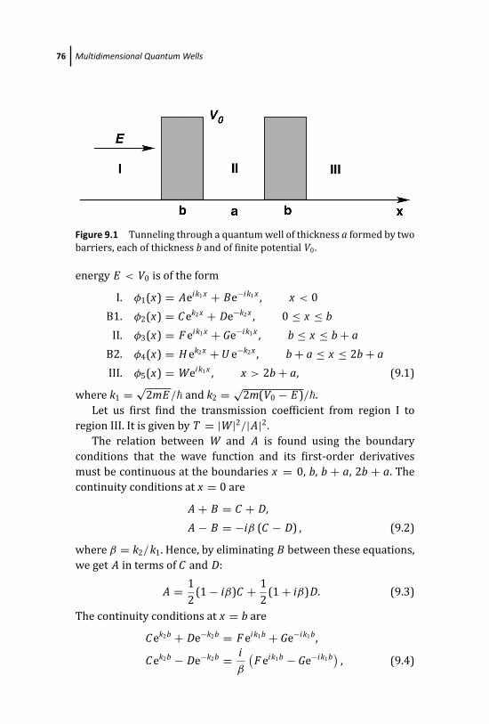
March 18, 2016 13:47 PSP Book - 9in x 6in Zbigniew-Ficek-tutsol
76 Multidimensional Quantum Wells
Figure 9.1 Tunneling through a quantum well of thickness a formed by two
barriers, each of thickness b and of finite potential V0.
energy E < V0 is of the form
I. φ1(x) = Aeik1 x + Be−ik1 x , x < 0
B1. φ2(x) = C ek2 x + De−k2 x , 0 ≤ x ≤ b
II. φ3(x) = F eik1 x + Ge−ik1 x , b ≤ x ≤ b + a
B2. φ4(x) = H ek2 x + U e−k2 x , b + a ≤ x ≤ 2b + a
III. φ5(x) = Weik1 x , x > 2b + a, (9.1)
where k1 = √2mE/� and k2 = √
2m(V0 − E )/�.
Let us first find the transmission coefficient from region I to
region III. It is given by T = |W|2/|A|2.
The relation between W and A is found using the boundary
conditions that the wave function and its first-order derivatives
must be continuous at the boundaries x = 0, b, b + a, 2b + a. The
continuity conditions at x = 0 are
A + B = C + D,
A − B = −iβ (C − D) , (9.2)
where β = k2/k1. Hence, by eliminating B between these equations,
we get A in terms of C and D:
A = 1
2(1 − iβ)C + 1
2(1 + iβ)D. (9.3)
The continuity conditions at x = b are
C ek2b + De−k2b = F eik1b + Ge−ik1b,
C ek2b − De−k2b = iβ
(F eik1b − Ge−ik1b) , (9.4)
March 18, 2016 13:47 PSP Book - 9in x 6in Zbigniew-Ficek-tutsol
Multidimensional Quantum Wells 77
from which we find C and D in terms of F and G
2C ek2b =(
1 + iβ
)F eik1b +
(1 − i
β
)Ge−ik1b,
2De−k2b =(
1 − iβ
)F eik1b +
(1 + i
β
)Ge−ik1b. (9.5)
Hence
C = i2β
[(1 − iβ) F eik1b − (1 + iβ) Ge−ik1b] e−k2b,
D = − i2β
[(1 + iβ) F eik1b − (1 − iβ) Ge−ik1b] ek2b. (9.6)
Substituting into Eq. (9.3), we get A in terms of F and G:
A = − i2β
{[(1 − β2
)sinh(k2b) + 2iβ cosh(k2b)
]F eik1b
− (1 + β2
)sinh(k2b)Ge−ik1b} , (9.7)
where we have used the relations
cosh α = 1
2
(eα + e−α
), sinh α = 1
2
(eα − e−α
), α = k2b.
(9.8)
The continuity conditions at x = b + a are
F eik1(b+a) + Ge−ik1(b+a) = H ek2(b+a) + U e−k2(b+a),
F eik1(b+a) − Ge−ik1(b+a) = −iβ(
H ek2(b+a) − U e−k2(b+a))
, (9.9)
which give
F eik1b = 1
2
[(1 − iβ) H ek2(b+a) + (1 + iβ) U e−k2(b+a)
]e−ik1a ,
Ge−ik1b = 1
2
[(1 + iβ) H ek2(b+a) + (1 − iβ) U e−k2(b+a)
]eik1a . (9.10)
The continuity conditions at x = 2b + a are
H ek2(2b+a) + U e−k2(2b+a) = Weik1(2b+a),
H ek2(2b+a) − U e−k2(2b+a) = iβ
Weik1(2b+a), (9.11)
from which we find H and U in terms of W:
H ek2(b+a) = i2β
(1 − iβ) Weik1(2b+a)−k2b,
U e−k2(b+a) = − i2β
(1 + iβ) Weik1(2b+a)+k2b, (9.12)
March 18, 2016 13:47 PSP Book - 9in x 6in Zbigniew-Ficek-tutsol
78 Multidimensional Quantum Wells
Substituting Eq. (9.12) into Eq. (9.10), we get
F eik1b = − i2β
[(1 − β2
)sinh(k2b) + 2iβ cosh(k2b)
]We2ik1b,
Ge−ik1b = − i2β
(1 + β2
)sinh(k2b)We2ik1(a+b). (9.13)
Substituting Eq. (9.13) into Eq. (9.7), we get A in terms of W:
A = − 1
4β2
[(1 − β2
)sinh(k2b) + 2iβ cosh(k2b)
]2We2ik1b
+ 1
4β2
(1 + β2
)2sinh2(k2b)We2ik1(a+b), (9.14)
which can be written as
4β2 Ae−2ik1b
W= − [(
1 − β2)
sinh(k2b) + 2iβ cosh(k2b)]2
+ (1 + β2
)2sinh2(k2b)e2ik1a
= 4β2
[cosh(k2b) + i
(β2 − 1
)2β
sinh(k2b)
]2
+4β2
(1 + β2
2β
)2
sinh2(k2b)e2ik1a . (9.15)
Hence, the ratio W/A required for the transmission coefficient is of
the form
WA
= e−2ik1b
(cosh α + iγ sinh α)2 + η2e2iu sinh2 α, (9.16)
where for clarity of expression, we have introduced the notations
α = k2b, u = k1a, γ = β2 − 1
2β, η = β2 + 1
2β. (9.17)
Since the denominator in Eq. (9.16) is the sum of squares of two
terms, we may use the relation a2 + b2 = (a + ib)(a − ib) and write
the ratio W/A as
WA
= e−2ik1b[cosh α + i(γ + ηeiu) sinh α
] [cosh α + i(γ − ηeiu) sinh α
] .
(9.18)
It is not difficult to show that the ratio is maximum when eiu = ±1.
This happens when
u = k1a = nπ, n = 0, 1, 2, . . . (9.19)
March 18, 2016 13:47 PSP Book - 9in x 6in Zbigniew-Ficek-tutsol
Multidimensional Quantum Wells 79
Since k1 = √2mE/�, we have evidence that the condition (9.19)
corresponds to discrete energy levels of the well:
k1a = nπ ⇒√
2mE�2
a = nπ ⇒ E = n2 π2�
2
2ma2. (9.20)
Thus, under the condition that the energy of the electron corre-
sponds to the energy levels of the well, the transmission through the
well is maximum with the transmission rate
|T |2 = 1[cosh2 α + (γ + η)2 sinh2 α
][cosh2 α + (γ − η)2 sinh2 α
]= 1
1 + η2 sinh2(2α), (9.21)
where we have used the relation cosh2 α = 1 + sinh2 α.
Problem 9.2
Find the number of wave functions (energy states) of a particle in a
quantum well of sides of equal lengths corresponding to energy
E = 9π2�
2
2ma2, (9.22)
i.e., for the combination of n1, n2, and n3 whose squares sum to 9.
Solution
To obtain the number of wave functions, we need to find the number
of different trios of integers (n1, n2, n3) whose squares sum to 9:
n21 + n2
2 + n23 = 9. (9.23)
This can be obtained from
n1 n2 n3
2 2 1
2 1 2
1 2 2 (9.24)
Thus, there are three wave functions corresponding to the energy
(9.22).
March 18, 2016 13:47 PSP Book - 9in x 6in Zbigniew-Ficek-tutsol
80 Multidimensional Quantum Wells
Problem 9.3
Find all energy states of a particle confined inside a three-
dimensional box with energies
E = 15π2
�2
2ma2. (9.25)
Indicate the degeneracy of each energy level.
Solution
The energy states are characterized by a trio of integers n1, n2, n3
whose sum of squares does not exceed 15.
E = (n21 + n2
2 + n23)E0 ≤ 15E0, (9.26)
where E0 = π2�
2/(2ma2).
The number of energy states, their energies, and their degen-
eracy are obtained with the following combinations of the integer
numbers. Note that ni cannot exceed 3 to have the sum of squares
not exceeding 15. The energy levels of the corresponding energies
are
E/E0 n1 n2 n3 Degeneracy
3 1 1 1 1
6 2 1 1 3
9 2 2 1 3
11 3 1 1 3
12 2 2 2 1
14 3 2 1 6 (9.27)
Thus, there are six energy states whose energies do not exceed
E = 15E0. Each energy state is characterized by a trio of integers,
which may be rearranged to give another state of the same energy.
For example, the trio (1, 1, 1) cannot be rearranged, so the lowest
energy state of energy E = 3E0 is a singlet. The trio (2, 1, 1) can be
rearranged to (1, 2, 1) and (1, 1, 2), so the state of energy E = 6E0
is a triplet.
March 18, 2016 13:47 PSP Book - 9in x 6in Zbigniew-Ficek-tutsol
Chapter 10
Linear Operators and Their Algebra
Problem 10.2
Let A, B , C be arbitrary linear operators. Prove that
(a)[
A B , C] = [
A, C]
B + A[
B , C]
,
(b)[
A,[
B , C]]+ [
B ,[C , A
]]+ [C ,[
A, B]] = 0 .
Solution (a)
The left-hand side of the relation can be written as
[A B , C
] = A BC − C A B . (10.1)
Consider now the right-hand side of the relation
[A, C
]B + A
[B , C
] = ( AC − C A)B + A(BC − C B)
= AC B − C A B + A BC − AC B
= A BC − C A B = L, (10.2)
as required.
Problems and Solutions in Quantum PhysicsZbigniew FicekCopyright c© 2016 Pan Stanford Publishing Pte. Ltd.ISBN 978-981-4669-36-8 (Hardcover), 978-981-4669-37-5 (eBook)www.panstanford.com
March 18, 2016 13:47 PSP Book - 9in x 6in Zbigniew-Ficek-tutsol
82 Linear Operators and Their Algebra
Solution (b)
Consider each of the commutators separately
(i)[
A,[
B , C]] = [
A, (BC − C B)] = A(BC − C B) − (BC − C B) A
= A BC − AC B − BC A + C B A.
(10.3)
(ii)[
B ,[C , A
]] = [B , (C A − AC )
] = B(C A − AC ) − (C A − AC )B
= BC A − B AC − C A B + AC B .
(10.4)
(iii)[C ,[
A, B]] = [
C , ( A B − B A)]= C ( A B − C A) − ( A B − B A)C
= C A B − C B A − A BC + B AC .
(10.5)
It is easy to see that the sum (i) + (ii) + (iii) = 0, as required.
Problem 10.3
Let [A, B
] = i�C and[
B , C] = i� A. (10.6)
Show that
B(
C + i A) = (
C + i A) (
B + �)
,
B(
C − i A) = (
C − i A) (
B − �)
. (10.7)
Solution
Since[
A, B] = i�C and
[B , C
] = i� A, we have
B(C + i A) = BC + i B A = i� A + C B + i( A B − i�C )
= (C + i A)B + �(C + i A) = (C + i A)(B + �),
(10.8)
as required.
March 18, 2016 13:47 PSP Book - 9in x 6in Zbigniew-Ficek-tutsol
Linear Operators and Their Algebra 83
Similarly
B(C − i A) = BC − i B A = i� A + C B − i( A B − i�C )
= (C − i A)B − �(C − i A) = (C − i A)(B − �),
(10.9)
as required.
These two relations show that[B , (C ± i A)
] = ±�(C ± i A). (10.10)
Problem 10.4
Show that
e A Be− A = B + 1
1!
[A, B
]+ 1
2!
[A,[
A, B]]+ 1
3!
[A,[
A,[
A, B]]]+ . . .
(10.11)
This formula shows that the calculation of complicated exponential-
type operator functions can be simplified to the calculation of a
series of commutators.
Solution
Expanding the exponents into the Taylor series
e± A = 1 ± 1
1!A + 1
2!A2 ± 1
3!A3 + . . . , (10.12)
we obtain
e A Be− A =(
1 + 1
1!A + 1
2!A2 + 1
3!A3 + . . .
)
B(
1 − 1
1!A + 1
2!A2 − 1
3!A3 + . . .
)
=(
B + 1
1!A B + 1
2!A2 B + 1
3!A3 B + . . .
)(
1 − 1
1!A + 1
2!A2 − 1
3!A3 + . . .
)
= B − B A + 1
2B A2 − 1
3!B A3 + . . . + A B − A B A + 1
2A B A2 + . . .
March 18, 2016 13:47 PSP Book - 9in x 6in Zbigniew-Ficek-tutsol
84 Linear Operators and Their Algebra
+1
2A2 B − 1
2A2 B A + 1
3!A3 B + . . .
= B + [A, B
]+ 1
2
(A2 B + B A2 − 2 A B A
)+ 1
3!
(A3 B − B A3 + 3 A B A2 − 3 A2 B A
)+ . . .
= B + [A, B
]+ 1
2
[A(
A B − B A)− (
A B − B A)
A]
+ 1
3!
[A(
A2 B + B A2)− (
A2 B + B A2)
A + 2 A B A2 − 2 A2 B A]
= B + [A, B
]+ 1
2
[A,[
A, B]]+ 1
3!
[A,[
A,[
A, B]]]+ . . .
= B + 1
1!
[A, B
]+ 1
2!
[A,[
A, B]]+ 1
3!
[A,[
A,[
A, B]]]+ . . .
(10.13)
Problem 10.5
Consider two arbitrary operators A and B . If A commutes with their
commutator[
A, B]:
(a) Prove that for a positive integer n
[An, B
] = nAn−1[
A, B]
. (10.14)
(b) Apply the commutation relation (a) to the special case of
A = x , B = px , and show that
[ f (x), px ] = i�d fdx
, (10.15)
assuming that f (x) can be expanded in a power series of the
operator x .
March 18, 2016 13:47 PSP Book - 9in x 6in Zbigniew-Ficek-tutsol
Linear Operators and Their Algebra 85
Solution (a)
We will prove this relation by induction. First, we check if this
relation is true for n = 1[A1, B
] = A0[
A, B] = [
A, B]
. (10.16)
Assume that the relation is true for n = k. We will prove that the
relation is true for n = k + 1, i.e.,[Ak+1, B
] = (k + 1) Ak [ A, B]
. (10.17)
Consider the left-hand side of the relation. Since
A[
A, B] = [
A, B]
A, (10.18)
we obtain
L = [Ak+1, B
]= Ak+1 B − B Ak+1 = Ak( A B − B A) + Ak B A − B Ak+1
= Ak [ A, B]+ ( Ak B − B Ak) A = Ak [ A, B
]+ [Ak, B
]A
= Ak [ A, B]+ kAk−1
[A, B
]A
= Ak [ A, B]+ kAk [ A, B
] = (k + 1) Ak [ A, B] = R , as required.
(10.19)
Solution (b)
Expanding f (x) into the Taylor series
f (x) =∑
n
1
n!
(dn fdxn
)x=0
xn, (10.20)
we obtain
[ f (x), px ] =∑
n
1
n!
(dn fdxn
)x=0
[xn, px ] . (10.21)
Now, applying the commutation relation from (a), we find∑n
1
n!
(dn fdxn
)x=0
[xn, px ] =∑
n
1
n!
(dn fdxn
)x=0
nxn−1 [x , px ] .
(10.22)
Since
[x , px ] = i�, (10.23)
March 18, 2016 13:47 PSP Book - 9in x 6in Zbigniew-Ficek-tutsol
86 Linear Operators and Their Algebra
we obtain∑n
1
n!
(dn fdxn
)x=0
nxn−1 [x , px ] =∑
n
1
n!
(dn fdxn
)x=0
nxn−1i�
= i�d
dx
(∑n
1
n!
(dn−1 fdxn−1
)x=0
nxn−1
)
= i�d
dx
(∑n
1
(n − 1)!
(dn−1 fdxn−1
)x=0
xn−1
). (10.24)
By substituting n − 1 = k, we get
i�d
dx
(∑n
1
(n − 1)!
(dn−1 fdxn−1
)x=0
xn−1
)
= i�d
dx
(∑k
1
k!
(dk fdxk
)x=0
xk
)= i�
d fdx
. (10.25)
Problem 10.7
Determine if the function φ = eax sin x , where a is a real constant, is
an eigenfunction of the operator d/dx and d2/dx2. If it is, determine
any eigenvalue.
Solution
The function φ is an eigenfunction of an operator A if
Aφ = αφ , (10.26)
where α is an eigenvalue.
We wish to find if the function φ is an eigenfunction of the
operators d/dx and d2/dx2.
Calculate
dφ
dxand
d2φ
dx2. (10.27)
Since
dφ
dx= aeax sin x + eax cos x = aφ + eax cos x , (10.28)
March 18, 2016 13:47 PSP Book - 9in x 6in Zbigniew-Ficek-tutsol
Linear Operators and Their Algebra 87
we see that
dφ
dx�= αφ for all a. (10.29)
From this result we see that φ is not an eigenfunction of the operator
d/dx .
Consider now the operator d2/dx2. Since
d2φ
dx2= a2eax sin x + aeax cos x + aeax cos x − eax sin x
= (a2 − 1)φ + 2aeax cos x , (10.30)
we can identify that for a = 0, φ is an eigenfunction of d2/dx2 with
an eigenvalue α = −1.
Problem 10.9
Calculate the expectation value of the x coordinate of a particle in
the energy state En of a one-dimensional box.
Solution
The expectation value of x is
〈x〉 =∫
φ∗(x)xφ(x)dx , (10.31)
where φ(x) is the wave function of the particle.
Since
φ(x) = φn(x) =√
2
asin
(nπ
ax)
, for 0 ≤ x ≤ a, (10.32)
March 18, 2016 13:47 PSP Book - 9in x 6in Zbigniew-Ficek-tutsol
88 Linear Operators and Their Algebra
and φ(x) is zero for x < 0 and x > a, we obtain
〈x〉 =∫
φ∗(x)xφ(x)dx = 2
a
∫ a
0
dx x sin2(nπ
ax)
= 1
a
∫ a
0
dx x[
1 − cos
(2nπ
ax)]
= 1
a
∫ a
0
dx[
x − x cos
(2nπ
ax)]
= 1
a
∫ a
0
dx x − 1
a
∫ a
0
dx x cos
(2nπ
ax)
= 1
a1
2x2
∣∣∣∣a
0
− 1
a
{− a2
(2nπ)2
[cos
(2nπ
ax)
+ 2nπxa
sin
(2nπ
ax)]a
0
}.
(10.33)
Since cos(2nπ) = cos 0 = 1 and sin(2nπ) = sin 0 = 0, it follows
that
〈x〉 = 1
2a, (10.34)
independent of n. Physically, this value results from the fact that the
wave function of the particle is symmetric about x = a/2 for all n.
Note, the expectation value is not equal to the most probable value,
which is given by |φ(x)|2.
Problem 10.11
For a particle in an infinite square well potential represented by
the position x and momentum px operators, check the uncertainty
principle xpx ≥ �/2 for n = 1, where x =√
〈x2〉 − 〈x〉2 and
px = √〈 p2x 〉 − 〈 px〉2.
Solution
For n = 1 the wave function of the particle in the infinite square well
potential is given by
φ1(x) =√
2
ae
ika2 sin
[π
a
(x − a
2
)], (10.35)
March 18, 2016 13:47 PSP Book - 9in x 6in Zbigniew-Ficek-tutsol
Linear Operators and Their Algebra 89
which can be written as
φ1(x) =√
2
ae
ika2 cos
(π
ax)
. (10.36)
First, calculate the average 〈x〉. From the definition of the expecta-
tion value (average), we have
〈x〉 =∫
φ∗1(x)xφ1(x)dx = 2
a
∫ a/2
−a/2
dx x cos2(π
ax)
. (10.37)
The integral is zero, as the function under the integral is an odd
function and the integral is taken over a range that is centered about
the origin. Thus, 〈x〉 = 0.
We now calculate 〈x2〉. From the definition of the expectation
value, we get
〈x2〉 =∫
φ∗1(x)x2φ1(x)dx = 2
a
∫ a/2
−a/2
dx x2 cos2(π
ax)
= 4
a
∫ a/2
0
dx x2 cos2(π
ax)
= 2
a
∫ a/2
0
dx x2
[1 + cos
(2π
ax)]
= 2
a
[∫ a/2
0
dx x2 +∫ a/2
0
dx x2 cos
(2π
ax)]
. (10.38)
In the second integral, we replace 2αx by z, where α = π/a, and then
integrating by parts, we obtain
〈x2〉 = 2
a
[∫ a/2
0
dx x2 + 1
8α3
∫ π
0
dz z2 cos z]
= 2
a
[x3
3
∣∣∣∣a/2
0
+ 1
8α3
(2z cos z + (z2 − 2) sin z
)∣∣π0
]
= 2
a
[a3
24+ 1
8α3(−2π)
]= 2
a
(a3
24− π
4
a3
π3
)= a2
2π2
(π2
6− 1
).
(10.39)
Hence, the variance x is
x =√
〈x2〉 − 〈x〉2 = a2π
√2
(π2
6− 1
). (10.40)
Calculate now 〈 px〉. Since
px = −i�d
dx, (10.41)
March 18, 2016 13:47 PSP Book - 9in x 6in Zbigniew-Ficek-tutsol
90 Linear Operators and Their Algebra
and
pxφ1(x) = −i�dφ1(x)
dx= −i�
√2
ae
ika2 α cos(αx), (10.42)
we obtain
〈 px〉 =∫
φ∗1(x) pxφ1(x)dx = −i�
2
a
∫ a/2
−a/2
dx cos αx (−α sin αx)
= 1
2i�α
∫ a/2
−a/2
dx sin(2αx). (10.43)
Since the function under the integral is an odd function and the
integral is taken over a range which is centered about the origin, the
integral is zero. Thus,
〈 px〉 = 0. (10.44)
Calculate 〈 p2x 〉:
〈 p2x 〉 =
∫φ∗
1(x) p2x φ1(x)dx = −�
2 2
a
∫ a/2
−a/2
dx cos(αx)d2
dx2cos(αx)
= �2α2 2
a
∫ a/2
−a/2
dx cos2(αx). (10.45)
However,∫ a/2
−a/2
dx cos2(αx) = 1
2
∫ a/2
−a/2
dx [1 + cos(2αx)] = a2
, (10.46)
and therefore
〈 p2x 〉 = �
2α2. (10.47)
Hence
px = α� = π�
a. (10.48)
Combining this result with that for x gives
xpx = a2π
√2
(π2
6− 1
)π�
a= �
2
√2
(π2
6− 1
). (10.49)
But, since √2
(π2
6− 1
)> 1, (10.50)
it follows that
xpx >�
2, (10.51)
i.e., the uncertainty principle is satisfied.
March 18, 2016 13:47 PSP Book - 9in x 6in Zbigniew-Ficek-tutsol
Linear Operators and Their Algebra 91
Problem 10.12
The expectation value of an arbitrary operator A in the state φ(x) is
given by
〈 A〉 =∫
φ∗(x) Aφ(x)dx . (10.52)
(a) Calculate expectation values (i) 〈x px〉, (i i) 〈 px x〉, and
(i i i) (〈x px〉 + 〈 px x〉)/2 of the product of position (x = x) and
momentum ( px = −i� ddx ) operators of a particle represented
by the wave function
φ(x) =√
2
asin
(πxa
), (10.53)
where 0 ≤ x ≤ a.
(b) The operators x and px are Hermitian. Which of the products
(i) x px , (i i) px x , and (i i i) (x px + px x)/2 are Hermitian?
(c) Explain, which of the results of (a) are acceptable as the
expectation values of physical quantities.
Solution (a)
(i) Consider the expectation value of x px in the state φ(x):
〈x px〉 =∫
φ∗(x)x pxφ(x)dx
= −i�2
a
∫ a
0
dx sin(πx
a
)x
ddx
sin(πx
a
)
= −i2π�
a2
∫ a
0
dx sin(πx
a
)x cos
(πxa
)
= −iπ�
a2
∫ a
0
dx x sin
(2πx
a
). (10.54)
By making the substitution α = 2πx/a, the previous integral
then becomes
〈x px〉 = −iπ�
a2
∫ a
0
dx x sin
(2πx
a
)= −i
�
4π
∫ 2π
0
dα α sin α.
(10.55)
March 18, 2016 13:47 PSP Book - 9in x 6in Zbigniew-Ficek-tutsol
92 Linear Operators and Their Algebra
The integration over α is readily performed by parts to give
〈x px〉 = −i�
4π
[−α cos α|2π
0 +∫ 2π
0
dα cos α
]
= −i�
4π
[−2π + sin α|2π0
] = 1
2i�. (10.56)
The expectation value of x px is a complex number. It means that
x px is not, Hermitian operator. We will show it more explicitly
in part (b).
(ii) Calculate now the expectation value of px x in the state φ(x).
Calculations similar to those performed in (i) give
〈 px x〉 =∫
φ∗(x) px xφ(x)dx = −i�2
a
∫ a
0
dx sin(πx
a
) ddx
[x sin
(πxa
)]
= −i2�
a
∫ a
0
dx sin(πx
a
) [sin
(πxa
)+ π
ax cos
(πxa
)]
= −i2�
a
∫ a
0
dx sin2(πx
a
)− i
2π�
a2
∫ a
0
dx x sin(πx
a
)cos
(πxa
)
= −i2�
a
∫ a
0
dx sin2(πx
a
)− i
π�
a2
∫ a
0
dx x sin
(2πx
a
)
= −i�
a
∫ a
0
dx[
1 − cos
(2πx
a
)]− i
π�
a2
∫ a
0
dx x sin
(2πx
a
)
= −i� + 1
2i� = −1
2i�.
(10.57)
(iii) Since the expectation value is additive, tht expectation value of
(x px + px x)/2 is obtained simply by adding the results (i) and
(ii):⟨1
2(x px + px x)
⟩= 1
2(〈x px〉 + 〈 px x〉) = 1
2
(1
2i� − 1
2i�)
= 0.
(10.58)
Solution (b)
From the definition, an operator A is Hermitian if A† = A.
(i) Consider a Hermitian conjugate of x px . Since x and px are
Hermitian operators and they do not commute, we get
(x px )† = p†x x† = px x �= x px . (10.59)
March 18, 2016 13:47 PSP Book - 9in x 6in Zbigniew-Ficek-tutsol
Linear Operators and Their Algebra 93
Hence, x px is not Hermitian. It is interesting that a product of
two Hermitian operators does not have to be Hermitian.
(ii) Consider px x . A Hermitian conjugate of px x is
( px x)† = x† p†x = x px �= px x . (10.60)
Hence, px x is not Hermitian.
(iii) Taking a Hermitian conjugate of (x px + px x)/2 and using the
results of (i) and (ii), we find
[(x px + px x)/2]† = (p†
x x† + x† p†x
)/2 = ( px x + x px )/2
= (x px + px x)/2. (10.61)
Hence, (x px + px x)/2 is Hermitian.
Solution (c)
Physical quantities are represented by Hermitian operators. Hence,
only (iii) 〈(x px + px x)/2〉 is acceptable as the expectation value of a
physical quantity.

This page intentionally left blankThis page intentionally left blank
March 18, 2016 13:47 PSP Book - 9in x 6in Zbigniew-Ficek-tutsol
Chapter 11
Dirac Bra-Ket Notation
Problem 11.1
Useful application of the completeness relation
As we have mentioned in the chapter, the completeness relation
is very useful in calculations involving operators and state vectors.
Consider the following example.
Let Ail and Bl j be matrix elements of two arbitrary operators Aand B in a basis of orthonormal vectors. Show, using the complete-
ness relation, that matrix elements of the product operator A B in
the same orthonormal basis can be found from the multiplication of
the matrix elements Ail and Bl j as
(A B
)i j =
n∑l=1
Ail Bl j . (11.1)
Solution
The completeness relation for a set of orthonormal states |φi 〉n∑
i=1
|φi 〉〈φi | = 1, (11.2)
Problems and Solutions in Quantum PhysicsZbigniew FicekCopyright c© 2016 Pan Stanford Publishing Pte. Ltd.ISBN 978-981-4669-36-8 (Hardcover), 978-981-4669-37-5 (eBook)www.panstanford.com
March 18, 2016 13:47 PSP Book - 9in x 6in Zbigniew-Ficek-tutsol
96 Dirac Bra-Ket Notation
can be used to represent an arbitrary operator in terms of the
orthonormal states. Consider an operator C , which is a product of
two operators A and B:
C = A B . (11.3)
Multiplying the operator C by the unity given by Eq. (11.2) both on
the right and the left, we then obtain the operator in terms of the
projection operators |φi 〉〈φi | as
C =(∑
i
|φi 〉〈φi |)
C
⎛⎝∑
j
|φ j 〉〈φ j |⎞⎠
=∑i, j
〈φi |C |φ j 〉|φi 〉〈φ j | =∑i, j
ci j |φi 〉〈φ j |, (11.4)
where ci j = 〈φi |C |φ j 〉 are matrix elements of the operator C in
the basis of the states |φi 〉. Since C = A B , we can write ci j =〈φi | A B|φ j 〉 ≡ (
A B)
i j .
Applying the completeness relation in between the operators Aand B , we get
(A B
)i j = 〈φi | A B|φ j 〉 = 〈φi | A
(∑l
|φl〉〈φl |)
B|φ j 〉
=n∑
l=1
〈φi | A|φl〉〈φl |B|φ j 〉 =n∑
l=1
Ail Bl j . (11.5)
Thus, matrix elements of the product operator A B in an orthonor-
mal basis are equal to the product of the matrix elements Ail and Bl j
of the operators A and B represented in the same basis.
Problem 11.2
Eigenvalues of the projection operator
Show that the eigenvalues of the projection operator Pnn are 0 or 1.
March 18, 2016 13:47 PSP Book - 9in x 6in Zbigniew-Ficek-tutsol
Dirac Bra-Ket Notation 97
Solution
Suppose that a state |m〉 is an eigenstate of the projection operator
with an eigenvalue α:
Pnn|m〉 = α|m〉. (11.6)
Since Pnn = |n〉〈n|, we have
Pnn|m〉 = |n〉〈n|m〉 = |n〉δnm = α|m〉. (11.7)
Multiplying both sides from the left by 〈m|, we get
〈m|n〉δnm = δ2nm = α. (11.8)
For n = m, δnm = 1, whereas for n �= m, δnm = 0. Thus, α = 0, 1.
Problem 11.3
Sum of two diagonal projection operators
Let Pnn and Pmm be diagonal projection operators. Show that the sum
Pnn+ Pmm is a diagonal projection operator if and only if Pnn Pmm = 0.
Solution
A diagonal projection operator has the property P 2kk = Pkk. Suppose
that Pkk = Pnn + Pmm. Then
P 2kk = (Pnn+Pmm)(Pnn+Pmm) = Pnn Pnn+Pnn Pmm+Pmm Pnn+Pmm Pmm.
(11.9)
Since Pnn Pnn = Pnn and Pmm Pmm = Pmm, we have
P 2kk = Pnn + Pnn Pmm + Pmm Pnn + Pmm. (11.10)
Hence, P 2kk = Pkk only if Pnn Pmm = 0.

This page intentionally left blankThis page intentionally left blank
March 18, 2016 13:47 PSP Book - 9in x 6in Zbigniew-Ficek-tutsol
Chapter 12
Matrix Representations
Problem 12.1
Eigenvalues and eigenvectors of Hermitian operators.
(a) Consider two Hermitian operators A and B that have the same
complete set of eigenfunctions φn. Show that the operators
commute.
(b) Suppose two Hermitian operators have the matrix representa-
tion:
A =⎡⎣a 0 0
0 −a 0
0 0 −a
⎤⎦ , B =
⎡⎣ b 0 0
0 0 ib0 −ib 0
⎤⎦ , (12.1)
where a and b are real numbers.
(i) Calculate the eigenvalues of A and B .
(ii) Show that A and B commute.
(iii) Determine a complete set of common eigenfunctions.
Problems and Solutions in Quantum PhysicsZbigniew FicekCopyright c© 2016 Pan Stanford Publishing Pte. Ltd.ISBN 978-981-4669-36-8 (Hardcover), 978-981-4669-37-5 (eBook)www.panstanford.com
March 18, 2016 13:47 PSP Book - 9in x 6in Zbigniew-Ficek-tutsol
100 Matrix Representations
Solution (a)
Assume that φn are eigenfunctions of A with corresponding eigen-
values αn, and eigenfunctions of B with corresponding eigenvalues
βn. Then
A Bφn = A (βnφn) = βn Aφn = βnαnφn. (12.2)
Similarly
B Aφn = B (αnφn) = αn Bφn = αnβnφn. (12.3)
Hence
A Bφn − B Aφn = [A, B
]φn = (βnαn − αnβn) φn = 0. (12.4)
Consequently,[
A, B] = 0.
Solution (b)
(i) Consider an eigenvalue equation for A:⎛⎝a 0 0
0 −a 0
0 0 −a
⎞⎠⎛⎝ c1
c2
c3
⎞⎠ = λ
⎛⎝ c1
c2
c3
⎞⎠ , (12.5)
which can be written as⎛⎝a − λ 0 0
0 −a − λ 0
0 0 −a − λ
⎞⎠⎛⎝ c1
c2
c3
⎞⎠ = 0. (12.6)
This equation has nonzero solutions when the determinant of the
matrix is zero, i.e., when∣∣∣∣∣∣a − λ 0 0
0 −a − λ 0
0 0 −a − λ
∣∣∣∣∣∣ = 0. (12.7)
From this we find a cubic equation
(λ − a)(λ + a)2 = 0. (12.8)
The roots of the cubic equation are
λ1 = a, λ2 = −a, λ3 = −a. (12.9)
March 18, 2016 13:47 PSP Book - 9in x 6in Zbigniew-Ficek-tutsol
Matrix Representations 101
Thus, the eigenvalues of the matrix A are λ1 = a and λ2, 3 = −a.
Note that the eigenvalues λ2 and λ3 are degenerated.
Consider now an eigenvalue equation for B:⎛⎝ b 0 0
0 0 ib0 −ib 0
⎞⎠⎛⎝ c1
c2
c3
⎞⎠ = λ
⎛⎝ c1
c2
c3
⎞⎠ . (12.10)
The equation can be written as⎛⎝b − λ 0 0
0 −λ ib0 −ib −λ
⎞⎠⎛⎝ c1
c2
c3
⎞⎠ = 0. (12.11)
This equation has nonzero solutions when the determinant of the
matrix is zero, i.e., when∣∣∣∣∣∣b − λ 0 0
0 −λ ib0 −ib −λ
∣∣∣∣∣∣ = 0. (12.12)
From this we find a cubic equation
(λ2 − b2)(λ − b) = 0. (12.13)
The roots of the cubic equation are
λ1 = b, λ2 = −b, λ3 = b. (12.14)
Thus, the eigenvalues of the matrix B are λ1, 3 = b and λ2 =−b. Similar to the operator A, two eigenvalues λ1 and λ2 are
degenerated.
(ii) Consider the commutator [ A, B] = A B − B A. First, we calculate
A B and find
A B =⎛⎝a 0 0
0 −a 0
0 0 −a
⎞⎠⎛⎝ b 0 0
0 0 ib0 −ib 0
⎞⎠ =
⎛⎝ab 0 0
0 0 −iab0 iab 0
⎞⎠ . (12.15)
Next, we calculate B A and find
B A =⎛⎝ b 0 0
0 0 ib0 −ib 0
⎞⎠⎛⎝a 0 0
0 −a 0
0 0 −a
⎞⎠ =
⎛⎝ab 0 0
0 0 −iab0 iab 0
⎞⎠ . (12.16)
Hence A B = B A. Thus, A and B commute.
March 18, 2016 13:47 PSP Book - 9in x 6in Zbigniew-Ficek-tutsol
102 Matrix Representations
(iii) Since the operators A and B commute, they have common
eigenfunctions. Therefore, it is enough to find the eigenfunctions of
either A or B . Lets find the eigenfunctions of A.
Notice that the matrix A is diagonal. This means that the basis
states φ1, φ2, φ3 are eigenstates (eigenfunctions) of the operator A.
We have showed in (ii) that the operators A and B commute,
so they have common eigenfunctions. It means that φ1, φ2, φ3 are
also the eigenfunctions of the operator B . One could question this
statement: Matrix B is not diagonal: then how could φ1, φ2, φ3 be
the eigenstates of matrix B?
The answer is in the fact that matrix B has two degenerate
eigenvalues λ2 = λ3 = b. If two eigenfunctions φ2 and φ3 of an
operator B are degenerated, then not only φ2 and φ3 are the
eigenfunctions of B , but also any linear combination of φ2 and φ3
is an eigenfunction of B . To prove this let us consider the eigenvalue
equation for matrix B:⎛⎝ b 0 0
0 0 ib0 −ib 0
⎞⎠⎛⎝ c1
c2
c3
⎞⎠ = λ
⎛⎝ c1
c2
c3
⎞⎠ . (12.17)
For λ = b, the eigenvalue equation is of the form⎛⎝ b 0 0
0 0 ib0 −ib 0
⎞⎠⎛⎝ c1
c2
c3
⎞⎠ = b
⎛⎝ c1
c2
c3
⎞⎠ . (12.18)
from which we find that
bc1 = bc1 and ibc3 = bc2. (12.19)
This means that φ1 is an eigenfunction of B with the eigenvalue b,
and a linear superposition
φb = ic3φ2 + c3φ3, (12.20)
is also an eigenfunction of the operator B with the eigenvalue b.
From the normalization condition, we find that c3 = 1/√
2, and
then the normalized eigenfunction φb is of the form
φb = 1√2
(iφ2 + φ3) . (12.21)
This clearly shows that in the case of degenerate eigenvalues of an
operator, not only φ1, φ2, . . . are eigenfunctions of the operator, but
an arbitrary combination of φ1, φ2, . . . is also an eigenfunction of the
operator.
March 18, 2016 13:47 PSP Book - 9in x 6in Zbigniew-Ficek-tutsol
Matrix Representations 103
Problem 12.2
The Rabi problem illustrates what are the energy states of an atomdriven by an external coherent (laser) field.
A laser field of frequency ωL drives a transition in an atom between
two atomic energy states |1〉 and |2〉. The states are separated by
the frequency ω0. The Hamiltonian of the system in the bases of the
atomic states is given by the matrix
H = �
(− 12 �
� 12
), (12.22)
where = ωL − ω0 is the detuning of the laser frequency from
the atomic transition frequency, and � is the Rabi frequency that
describes the strength of the laser field acting on the atom.
Find the energies and energy states of the system, the so-called
dressed states, which are, respectively, eigenvalues and eigenvectors
of the Hamiltonian H .
Solution
In general, the energy state of the system is a linear superposition of
the energy states |1〉 and |2〉:
|�〉 = c1|1〉 + c2|2〉, (12.23)
where c1 and c2 are unknown amplitudes, which are to be
determined solving an eigenvalue equation for the Hamiltonian H .
The eigenvalue equation for H is(− 12 �
� 12
)(c1
c2
)= λ
(c1
c2
), (12.24)
which can be written as(− 12 − λ �
� 12 − λ
)(c1
c2
)= 0. (12.25)
This equation has nonzero solutions when the determinant of the
matrix is zero, i.e., when∣∣∣∣− 12 − λ �
� 12 − λ
∣∣∣∣ = 0. (12.26)
March 18, 2016 13:47 PSP Book - 9in x 6in Zbigniew-Ficek-tutsol
104 Matrix Representations
From this we find a quadratic equation
λ2 − 1
42 − �2 = 0, (12.27)
whose roots are
λ1, 2 = ±√
1
42 + �2 ≡ ±�. (12.28)
The eigenvalues λ1, 2 of the Hamiltonian are the energies of the
system.
In order to find the energy states of the system, we have to
find the eigenvectors of the Hamiltonian corresponding to the two
eigenvalues, λ1 = � and λ2 = −�.
For λ1 = �, the eigenvalue equation is of the form(− 12 �
� 12
)(c1
c2
)= �
(c1
c2
), (12.29)
from which we find an equation relating the coefficients c1 and c2:
−1
2c1 + �c2 = �c1. (12.30)
From this relation, we find
c1 = �
� + 12
c2. (12.31)
Thus, the energy state of the system corresponding to the energy
λ1 = � is
|�1〉 = �
� + 12
c2|1〉 + c2|2〉. (12.32)
The undetermined coefficient c2 is found from the normalization
condition 〈�1|�1〉 = 1, which gives
c2 =√
� + 12
2�. (12.33)
Hence, the state |�1〉 takes the form
|�1〉 = �
� + 12
√� + 1
2
2�|1〉 +
√� + 1
2
2�|2〉
=√
�2
2�(� + 12)
|1〉 +√
� + 12
2�|2〉
=√
�2 − 142
2�(� + 12)
|1〉 +√
� + 12
2�|2〉
=√
� − 12
2�|1〉 +
√� + 1
2
2�|2〉. (12.34)
March 18, 2016 13:47 PSP Book - 9in x 6in Zbigniew-Ficek-tutsol
Matrix Representations 105
Similarly, for λ1 = −�, the eigenvalue equation is of the form(− 12 �
� 12
)(c1
c2
)= −�
(c1
c2
), (12.35)
from which we find an equation relating the coefficients c1 and c2:
−1
2c1 + �c2 = −�c1, (12.36)
From this relation, we find
c1 = −�
� − 12
c2. (12.37)
Thus, the energy state of the system corresponding to the energy
λ1 = −� is
|�2〉 = −�
� − 12
c2|1〉 + c2|2〉. (12.38)
From the normalization condition, 〈�2|�2〉 = 1, we readily find
c2 =√
� − 12
2�. (12.39)
Hence, the state |�2〉 takes the form
|�2〉 = −�
� − 12
√� − 1
2
2�|1〉 +
√� − 1
2
2�|2〉
= −√
�2
2�(� − 12)
|1〉 +√
� − 12
2�|2〉
= −√
�2 − 142
2�(� − 12)
|1〉 +√
� − 12
2�|2〉
= −√
� + 12
2�|1〉 +
√� − 1
2
2�|2〉. (12.40)
It is easy to check that the energy states |�1〉 and |�2〉 are
orthogonal, i.e., 〈�1|�2〉 = 0.
The energy states are linear superpositions of the atomic states.
The superpositions are induced by the laser field forcing the electron
to jump between the atomic states |1〉 and |2〉. It is often said that the
superpositions result from “dressing” the atom in the laser field. For
this reason, the states are called in the literature as dressed states of
the two-level system.

This page intentionally left blankThis page intentionally left blank
March 18, 2016 13:47 PSP Book - 9in x 6in Zbigniew-Ficek-tutsol
Chapter 13
Spin Operators and Pauli Matrices
Problem 13.1
Calculate the square ( �A · �S)2 of the scalar product of an arbitrary
vector �A and of the spin vector �S = Sx�i + Sy�j + Sz�k.
Solution
In the cartesian coordinates, �A = Ax�i + Ay�j + Az�k. Hence, the dot
product between �A and �S is
�A · �S = Ax Sx + Ay Sy + AzSz. (13.1)
Squaring �A · �S , we obtain(�A · �S
)2
= (Ax Sx + Ay Sy + AzSz
) (Ax Sx + Ay Sy + AzSz
)= A2
x S2x + Ax Ay Sx Sy + Ax AzSx Sz
+Ay Ax Sy Sx + A2y S2
y + Ay AzSy Sz
+Az Ax SzSx + Az Ay SzSy + A2z S2
z
= A2x S2
x + A2y S2
y + A2z S2
z + Ax Ay[Sx , Sy]++Ax Az[Sx , Sz]+ + Ay Az[Sy , Sz]+. (13.2)
Problems and Solutions in Quantum PhysicsZbigniew FicekCopyright c© 2016 Pan Stanford Publishing Pte. Ltd.ISBN 978-981-4669-36-8 (Hardcover), 978-981-4669-37-5 (eBook)www.panstanford.com
March 18, 2016 13:47 PSP Book - 9in x 6in Zbigniew-Ficek-tutsol
108 Spin Operators and Pauli Matrices
Since the components of the spin anticommute, i.e.,
[Sx , Sy]+ = [Sx , Sz]+ = [Sy , Sz]+ = 0 (13.3)
and
S2x = S2
y = S2z = 1
4�
2, (13.4)
we finally get(�A · �S
)2
= 1
4�
2(
A2x + A2
y + A2z
) = 1
4�
2| �A|2 = |�S|2| �A|2. (13.5)
Thus, ( �A · �S)2 is equal to the product of the squares of the vector �Aand the spin vector �S .
Problem 13.2
Calculate the squares of the spin components σ 2x , σ 2
y , and σ 2z , and
verify if the squares of the spin components can be simultaneously
measured with the same precision.
Solution
Calculate σ 2x :
σ 2x = σx σx =
(0 1
1 0
)(0 1
1 0
)=(
1 0
0 1
)= 1. (13.6)
Similarly
σ 2y = σyσy =
(0 −ii 0
)(0 −ii 0
)=(
1 0
0 1
)= 1, (13.7)
and
σ 2z = σzσz =
(1 0
0 −1
)(1 0
0 −1
)=(
1 0
0 1
)= 1. (13.8)
The squares of the spin components are unit operators. Hence,
they commute with each other. Therefore, the squares of the
spin components can be simultaneously measured with the same
precision.
March 18, 2016 13:47 PSP Book - 9in x 6in Zbigniew-Ficek-tutsol
Spin Operators and Pauli Matrices 109
Problem 13.3
Matrix representation of spin operators
The operators σx , σy , and σz representing the components of the
electron spin, can � be written in terms of the spin raising and spin
lowering operators σ+ and σ− as
σx = σ+ + σ−,
σy = (σ+ − σ−) / i,
σz = σ+σ− − σ−σ+. (13.9)
Let |1〉 and |2〉 the two eigenstates of the electron spin with
the eigenvalues −�/2 and +�/2, respectively, as determined in
the Stern–Gerlach experiment. The raising and lowering operators
satisfy the following relations:
σ+|1〉 = |2〉 , σ−|1〉 = 0,
σ+|2〉 = 0 , σ−|2〉 = |1〉. (13.10)
Using these relations, find the matrix representations (the Pauli
matrices) of the operators σx , σy , and σz in the basis of the states |1〉and |2〉.
Solution
Find first the matrix representation of σx . In the basis of the states
|2〉 and |1〉, the operator σx has a matrix representation of the form
σx =( 〈2|σx |2〉 〈2|σx |1〉
〈1|σx |2〉 〈1|σx |1〉)
. (13.11)
The matrix elements are
〈1|σx |1〉 = 〈1| (σ+ + σ−) |1〉 = 〈1|2〉 + 〈1|0 = 0 + 0 = 0,
〈1|σx |2〉 = 〈1| (σ+ + σ−) |2〉 = 〈1|0 + 〈1|1〉 = 0 + 1 = 1,
〈2|σx |1〉 = 〈2| (σ+ + σ−) |1〉 = 〈2|2〉 + 〈2|0 = 1 + 0 = 1,
〈2|σx |2〉 = 〈2| (σ+ + σ−) |2〉 = 〈2|0 + 〈2|1〉 = 0 + 0 = 0,
(13.12)
March 18, 2016 13:47 PSP Book - 9in x 6in Zbigniew-Ficek-tutsol
110 Spin Operators and Pauli Matrices
and then the matrix (13.11) takes the form
σx =(
0 1
1 0
). (13.13)
Similarly, in the basis of the states |2〉 and |1〉, the operator σy has a
matrix representation of the form
σy =( 〈2|σy|2〉 〈2|σy|1〉
〈1|σy|2〉 〈1|σy|1〉)
. (13.14)
Since
〈1|σy|1〉 = 〈1| (σ+ − σ−) / i |1〉 = (〈1|2〉 − 〈1|0)/ i = 0,
〈1|σy|2〉 = 〈1| (σ+ − σ−) / i |2〉 = (〈1|0 − 〈1|1〉)/ i = i,
〈2|σy|1〉 = 〈2| (σ+ − σ−) / i |1〉 = (〈2|2〉 − 〈2|0)/ i = −i,
〈2|σy|2〉 = 〈2| (σ+ − σ−) / i |2〉 = (〈2|0 − 〈2|1〉)/ i = 0, (13.15)
the matrix (13.14) takes the form
σy =(
0 −ii 0
). (13.16)
Finally, in the basis of the states |2〉 and |1〉, the operator σz has a
matrix representation of the form
σz =( 〈2|σz|2〉 〈2|σz|1〉
〈1|σz|2〉 〈1|σz|1〉)
. (13.17)
Since
〈1|σz|1〉 = 〈1| (σ+σ− − σ−σ+) |1〉 = 〈1|0 − 〈1|1〉 = −1,
〈1|σz|2〉 = 〈1| (σ+σ− − σ−σ+) |2〉 = 〈1|2〉 − 〈1|0 = 0,
〈2|σz|1〉 = 〈2| (σ+σ− − σ−σ+) |1〉 = 〈2|0 − 〈2||1〉 = 0,
〈2|σz|2〉 = 〈2| (σ+σ− − σ−σ+) |2〉 = 〈2|2〉 − 〈2|0 = 1, (13.18)
the matrix (13.17) takes the form
σz =(
1 0
0 −1
). (13.19)
March 18, 2016 13:47 PSP Book - 9in x 6in Zbigniew-Ficek-tutsol
Spin Operators and Pauli Matrices 111
Problem 13.4
Properties of the Pauli matrices
Consider the Pauli matrices representing the spin operators σx , σy ,
and σz in the basis of the states |1〉 and |2〉.
(a) Prove that the operators σx , σy , σz are Hermitian. This result
is what the student could expect as the operators represent a
physical (measurable) quantity, the electron spin.
(b) Show that each of the operators σx , σy , σz has eigenvalues
+1, −1. Determine the normalized eigenvectors of each. Are |1〉and |2〉 the eigenvectors of any of the matrices?
(c) Show that the operators σx , σy , σz obey the commutation
relations [σx , σy
] = 2i σz,
[σz, σx ] = 2i σy ,[σy , σz
] = 2i σx . (13.20)
If you recall the Heisenberg uncertainty relation, you will
conclude immediately that these commutation relations show
that the three components of the spin cannot be measured
simultaneously with the same precision.
(d) Calculate anticommutators[σx , σy
]+ , [σz, σx ]+ ,
[σy , σz
]+.
(e) Show that σ 2x = σ 2
y = σ 2z = 1. This result is a confirmation of the
conservation of the total spin of the system that the magnitude
of the total spin vector is constant.
(f) Write the operators σx , σy , and σz in terms of the projection
operators Pi j = |i〉〈 j |, (i, j = 1, 2).
Solution (a)
An operator (matrix) A is Hermitian if
〈φi | A|φ j 〉 = 〈φ j | A|φi 〉∗. (13.21)
It is easy to see that for all the matrices
〈φi |σn|φ j 〉 = 〈φ j |σn|φi 〉∗ , i, j = 1, 2, (13.22)
where n = x , y, z. Thus, the matrices σx , σy , σz are Hermitian.
March 18, 2016 13:47 PSP Book - 9in x 6in Zbigniew-Ficek-tutsol
112 Spin Operators and Pauli Matrices
Solution (b)
Consider an eigenvalue equation for σx :(0 1
1 0
)(c1
c2
)= λ
(c1
c2
), (13.23)
which can be written as(−λ 1
1 −λ)(
c1
c2
)= 0. (13.24)
This equation has nonzero solutions when the determinant of the
matrix is zero, i.e., when ∣∣∣∣−λ 1
1 −λ∣∣∣∣ = 0. (13.25)
From this we find a quadratic equation
λ2 − 1 = 0, (13.26)
whose solutions are
λ = ±1. (13.27)
Thus, the eigenvalues of the matrix σx are +1 and −1.
Now, we will find eigenvectors corresponding to the eigenvalues
λ = ±1.
For λ = 1, the eigenvalue equation is of the form(0 1
1 0
)(c1
c2
)=(
c1
c2
), (13.28)
from which we find
c1 = c2. (13.29)
Thus, the eigenvector of the matrix σx corresponding to the
eigenvalue +1 is of the form
|�x〉+1 = c1 (|φ1〉 + |φ2〉) . (13.30)
We find the coefficient c1 from the normalization condition
1 = +1〈 �x |�x〉+1 = (〈φ1| + 〈φ2|) c∗1c1 (|φ1〉 + |φ2〉)
= |c1|2 (〈φ1|φ1〉 + 〈φ1|φ2〉 + 〈φ2|φ1〉 + 〈φ2|φ2〉)
= |c1|2 (1 + 0 + 0 + 1) = 2|c1|2. (13.31)
March 18, 2016 13:47 PSP Book - 9in x 6in Zbigniew-Ficek-tutsol
Spin Operators and Pauli Matrices 113
Hence
c1 = 1√2
, (13.32)
and then the normalized eigenvector of σx corresponding to the
eigenvalue +1 is of the form
|�x〉+1 = 1√2
(|φ1〉 + |φ2〉) . (13.33)
Similarly, for λ = −1, the eigenvalue equation is of the form(0 1
1 0
)(c1
c2
)= −
(c1
c2
), (13.34)
from which we find that
c2 = −c1. (13.35)
Thus, the eigenvector of the matrix σx corresponding to the
eigenvalue −1 is of the form
|�x〉−1 = c1 (|φ1〉 − |φ2〉) . (13.36)
As usual, we find the coefficient c1 from the normalization condition
1 = −1〈 �x |�x〉−1 = (〈φ1| − 〈φ2|) c∗1c1 (|φ1〉 − |φ2〉)
= |c1|2 (〈φ1|φ1〉 − 〈φ1|φ2〉 − 〈φ2|φ1〉 + 〈φ2|φ2〉)
= |c1|2 (1 − 0 − 0 + 1) = 2|c1|2. (13.37)
Hence
c1 = 1√2
, (13.38)
and then the normalized eigenvector of σx corresponding to the
eigenvalue −1 is of the form
|�x〉−1 = 1√2
(|φ1〉 − |φ2〉) . (13.39)
In summary, the normalized eigenvectors of σx written in terms of
the orthonormal vectors |φ1〉 and |φ2〉 are of the form
|�x〉+1 = 1√2
(|φ1〉 + |φ2〉) ,
|�x〉−1 = 1√2
(|φ1〉 − |φ2〉) . (13.40)
Consider now the matrix σy .
March 18, 2016 13:47 PSP Book - 9in x 6in Zbigniew-Ficek-tutsol
114 Spin Operators and Pauli Matrices
The eigenvalue equation for σy is of the form(0 −ii 0
)(c1
c2
)= λ
(c1
c2
), (13.41)
which can be written as(−λ −ii −λ
)(c1
c2
)= 0. (13.42)
This equation has nonzero solutions when the determinant of the
matrix is zero, i.e., when ∣∣∣∣−λ −ii −λ
∣∣∣∣ = 0. (13.43)
From this we find that the determinant is equal to a quadratic
equation
λ2 − 1 = 0, (13.44)
whose solutions are
λ = ±1. (13.45)
Thus, the eigenvalues of the matrix σy are +1 and −1.
Now, we will find eigenvectors corresponding to the eigenvalues
λ = ±1.
For λ = 1, the eigenvalue equation is of the form(0 −ii 0
)(c1
c2
)=(
c1
c2
), (13.46)
from which we find
c1 = −ic2. (13.47)
Thus, the eigenvector of the matrix σy corresponding to the
eigenvalue +1 is of the form
|�y〉+1 = c1 (|φ1〉 + i |φ2〉) . (13.48)
As usual, we find the coefficient c1 from the normalization condition
1 = +1〈 �y|�y〉+1 = (〈φ1| − i〈φ2|) c∗1c1 (|φ1〉 + i |φ2〉)
= |c1|2 (〈φ1|φ1〉 + i〈φ1|φ2〉 − i〈φ2|φ1〉 + 〈φ2|φ2〉)
= |c1|2 (1 + i0 − i0 + 1) = 2|c1|2. (13.49)
March 18, 2016 13:47 PSP Book - 9in x 6in Zbigniew-Ficek-tutsol
Spin Operators and Pauli Matrices 115
Hence
c1 = 1√2
, (13.50)
and then the normalized eigenvector of σy corresponding to the
eigenvalue +1 is of the form
|�y〉+1 = 1√2
(|φ1〉 + i |φ2〉) . (13.51)
Similarly, for λ = −1, the eigenvalue equation is of the form(0 −ii 0
)(c1
c2
)= −
(c1
c2
), (13.52)
from which we find
c2 = −ic1. (13.53)
Thus, the eigenvector of the matrix σy corresponding to the
eigenvalue −1 is of the form
|�y〉−1 = c1 (|φ1〉 − i |φ2〉) . (13.54)
As usual, we find the coefficient c1 from the normalization condition
1 = −1〈 �y|�y〉−1 = (〈φ1| + i〈φ2|) c∗1c1 (|φ1〉 − i |φ2〉)
= |c1|2 (〈φ1|φ1〉 − i〈φ1|φ2〉 + i〈φ2|φ1〉 + 〈φ2|φ2〉)
= |c1|2 (1 + i0 − i0 + 1) = 2|c1|2. (13.55)
Hence
c1 = 1√2
, (13.56)
and then the normalized eigenvector of σy corresponding to the
eigenvalue −1 is of the form
|�y〉−1 = 1√2
(|φ1〉 − i |φ2〉) . (13.57)
In summary, the normalized eigenvectors of σy written in terms of
the orthonormal vectors |φ1〉 and |φ2〉 are of the form
|�y〉+1 = 1√2
(|φ1〉 + i |φ2〉) ,
|�y〉−1 = 1√2
(|φ1〉 − i |φ2〉) . (13.58)
Finally, consider the matrix σz.
It is easily to see that the matrix σz is diagonal. Thus, the basis
vectors |φ1〉 and |φ2〉 are the eigenvectors of σz. Since
〈φ1|σz|φ1〉 = 1 and 〈φ2|σz|φ2〉 = −1, (13.59)
we see that |φ1〉 is an eigenvector of σz with eigenvalue +1, and |φ2〉is an eigenvector of σz with eigenvalue −1.
March 18, 2016 13:47 PSP Book - 9in x 6in Zbigniew-Ficek-tutsol
116 Spin Operators and Pauli Matrices
Solution (c)
Consider the commutator[σx , σy
]:
[σx , σy
] = σx σy − σyσx
=(
0 1
1 0
)(0 −ii 0
)−(
0 −ii 0
)(0 1
1 0
)
=(
i 0
0 −i
)−(−i 0
0 i
)=(
2i 0
0 −2i
)
= 2i(
1 0
0 −1
)= 2i σz. (13.60)
Similarly,
[σz, σx ] = σzσx − σx σz
=(
1 0
0 −1
)(0 1
1 0
)−(
0 1
1 0
)(1 0
0 −1
)
=(
0 1
−1 0
)−(
0 −1
1 0
)=(
0 2
−2 0
)
= 2i(
0 −ii 0
)= 2i σy , (13.61)
and
[σy , σz
] = σyσz − σzσy
=(
0 −ii 0
)(1 0
0 −1
)−(
1 0
0 −1
)(0 −ii 0
)
=(
0 ii 0
)−(
0 −i−i 0
)=(
0 2i2i 0
)
= 2i(
0 1
1 0
)= 2i σx . (13.62)
March 18, 2016 13:47 PSP Book - 9in x 6in Zbigniew-Ficek-tutsol
Spin Operators and Pauli Matrices 117
Solution (d)
Consider the anticommutator[σx , σy
]+:[
σx , σy]+ = σx σy + σyσx
=(
0 1
1 0
)(0 −ii 0
)+(
0 −ii 0
)(0 1
1 0
)
=(
i 0
0 −i
)+(−i 0
0 i
)=(
0 0
0 0
)= 0 . (13.63)
Similarly,
[σz, σx ]+ = σzσx + σx σz
=(
1 0
0 −1
)(0 1
1 0
)+(
0 1
1 0
)(1 0
0 −1
)
=(
0 1
−1 0
)+(
0 −1
1 0
)=(
0 0
0 0
)= 0, (13.64)
and[σy , σz
]+ = σyσz + σzσy
=(
0 −ii 0
)(1 0
0 −1
)+(
1 0
0 −1
)(0 −ii 0
)
=(
0 ii 0
)+(
0 −i−i 0
)=(
0 0
0 0
)= 0. (13.65)
Hence, [σx , σy
]+ = [σz, σx ]+ = [
σy , σz]+ = 0. (13.66)
Solution (e)
Consider σ 2x :
σ 2x = σx σx =
(0 1
1 0
)(0 1
1 0
)=(
1 0
0 1
)= 1. (13.67)
Similarly,
σ 2y = σyσy =
(0 −ii 0
)(0 −ii 0
)=(
1 0
0 1
)= 1, (13.68)
March 18, 2016 13:47 PSP Book - 9in x 6in Zbigniew-Ficek-tutsol
118 Spin Operators and Pauli Matrices
and
σ 2z = σzσz =
(1 0
0 −1
)(1 0
0 −1
)=(
1 0
0 1
)= 1. (13.69)
Hence,
σ 2x = σ 2
y = σ 2z = 1. (13.70)
Solution (f)
As we have shown in lecture, an arbitrary operator A can be written
in terms of the projector operators as
A =∑n, m
Amn|m〉〈n| =∑n, m
Amn Pmn. (13.71)
Thus, in the basis of the two orthonormal states |1〉, |2〉, the operator
σx can be written as
σx =2∑
n, m=1
σ xmn|m〉〈n| = σ x
11|1〉〈1| + σ x12|1〉〈2| + σ x
21|2〉〈1| + σ x22|2〉〈2|.(13.72)
Since
σ x11 = 〈1|σx |1〉 = 0, σ x
22 = 〈2|σx |2〉 = 0
σ x12 = 〈1|σx |2〉 = 1, σ x
21 = 〈2|σx |1〉 = 1, (13.73)
we find
σx = |1〉〈2| + |2〉〈1|. (13.74)
Following the same procedure, we find that the operator σy can be
written as
σy =2∑
n, m=1
σ ymn|m〉〈n| = σ
y11|1〉〈1| + σ
y12|1〉〈2| + σ
y21|2〉〈1| + σ
y22|2〉〈2|.(13.75)
Since
σy
11 = 〈1|σy|1〉 = 0, σy
22 = 〈2|σy|2〉 = 0
σy
12 = 〈1|σy|2〉 = −i, σy
21 = 〈2|σy|1〉 = i, (13.76)
March 18, 2016 13:47 PSP Book - 9in x 6in Zbigniew-Ficek-tutsol
Spin Operators and Pauli Matrices 119
we find
σy = −i (|1〉〈2| − |2〉〈1|) . (13.77)
Similarly, the operator σz can be written as
σz =2∑
n, m=1
σ zmn|m〉〈n| = σ z
11|1〉〈1| + σ z12|1〉〈2| + σ z
21|2〉〈1| + σ z22|2〉〈2|.(13.78)
Since
σ z11 = 〈1|σz|1〉 = 1, σ z
22 = 〈2|σz|2〉 = −1
σ z12 = 〈1|σz|2〉 = 0, σ z
21 = 〈2|σz|1〉 = 0, (13.79)
we find that
σz = |1〉〈1| − |2〉〈2|. (13.80)

This page intentionally left blankThis page intentionally left blank
March 18, 2016 13:47 PSP Book - 9in x 6in Zbigniew-Ficek-tutsol
Chapter 14
Quantum Dynamics and Pictures
Problem 14.1
Consider a two-level atom of energy states |1〉 and |2〉 driven by a
laser field. The atom can be represented as a spin- 12
particle and the
laser field can be treated as a classical field. The Hamiltonian of the
system is given by
H = 1
2�ω0σz − 1
2i��
(σ+e−iωLt − σ−eiωLt) , (14.1)
where � is the Rabi frequency of the laser field, ω0 is the atomic
transition frequency, ωL is the laser frequency, and σz, σ+ and σ−
are the spin operators defined as
σz = |2〉〈2| − |1〉〈1|, σ+ = |2〉〈1|, σ− = |1〉〈2|. (14.2)
(a) Calculate the equation of motion for σ−.
(b) The equation of motion derived in (a) contains a time-
dependent coefficient. Find a unitary operator that transforms
σ− into ˆσ− whose equation of motion is free from time-
dependent coefficients.
Problems and Solutions in Quantum PhysicsZbigniew FicekCopyright c© 2016 Pan Stanford Publishing Pte. Ltd.ISBN 978-981-4669-36-8 (Hardcover), 978-981-4669-37-5 (eBook)www.panstanford.com
March 18, 2016 13:47 PSP Book - 9in x 6in Zbigniew-Ficek-tutsol
122 Quantum Dynamics and Pictures
Solution (a)
The equation of motion for an operator is found using the
Heisenberg equation of motion. For the operator σ−, the equation
of motion is given by
ddt
σ− = i�
[H , σ−] . (14.3)
Evaluating the commutator [H , σ−], we get
[H , σ−] = 1
2�ω0
[σz, σ−]− 1
2i��
[(σ+e−iωLt − σ−eiωLt) , σ−] .
(14.4)
Since[σz, σ−] = −2σ−,
[σ+, σ−] = σz,
[σ−, σ−] = 0, (14.5)
we get
[H , σ−] = −�ω0σ
− − 1
2i��σze−iωLt . (14.6)
Hence, the equation of motion for the operator σ− is of the form
ddt
σ− = −iω0σ− + 1
2�e−iωLtσz. (14.7)
The equation of motion is a differential equation with a time-
dependent coefficient �e−iωLt . It makes the equation difficult to
solve. It can be simplified to a differential equation with time-
independent coefficients by making a unitary transformation of the
operators.
Solution (b)
The time-dependent coefficient in Eq. (14.7) oscillates with fre-
quency ωL. Therefore, the unitary operator that transforms the
equation to an equation with time-independent coefficients should
involve the frequency ωL. Moreover, it should involve an operator
of the system whose commutator with σ− is equal to σ−. A unitary
operator that satisfies those requirements is of the form
U (t) = e12
iωLσzt . (14.8)
March 18, 2016 13:47 PSP Book - 9in x 6in Zbigniew-Ficek-tutsol
Quantum Dynamics and Pictures 123
Introducing a new “transformed” operator ˆσ− = U †(t)σ−U (t), we
find that the unitary operator U (t) transforms σ− into
ˆσ− = U †(t)σ−U (t)=(
1 − 1
2iωLσzt + . . .
)σ−
(1 + 1
2iωLσzt + . . .
)
=(
σ− − 1
2iωLσzσ
−t + . . .
)(1 + 1
2iωLσzt + . . .
)
= σ− + 1
2iωLtσ−σz − 1
2iωLtσzσ
− + . . .
= σ− − 1
2iωLt
[σz, σ−]+ . . . = σ− + iωLtσ− + . . .
= σ− (1 + iωLt + . . .) = σ−eiωLt . (14.9)
Hence, the equation of motion for ˆσ− is of the form
ddt
ˆσ− = ddt
(σ−eiωLt) =
(ddt
σ−)
e−iωLt + σ−(
ddt
eiωLt)
=(
−iω0σ− + 1
2�σze−iωLt
)eiωLt + iωLσ
−eiωLt
= −i (ω0 − ωL) σ−eiωLt + 1
2�σz = −i ˆσ− + 1
2�σz,
(14.10)
where = ω0 −ωL. The equation of motion for the transformed op-
erator is a differential equation with time-independent coefficients.
Problem 14.2
The Hamiltonian of the two-level atom interacting with a classical
laser field can be written as
H = H0 + V (t), (14.11)
where
H0 = 1
2�ω0σz
V (t) = −1
2i��
(σ+e−iωLt − σ−eiωLt) . (14.12)
(a) Transform V (t) into the interaction picture to find VI =U †
0 V (t)U 0.
(b) Find the equation of motion for σ− in the interaction picture, i.e.,
find the equation of motion for σ−I (t) = U †
I σ−U I .
March 18, 2016 13:47 PSP Book - 9in x 6in Zbigniew-Ficek-tutsol
124 Quantum Dynamics and Pictures
Solution (a)
With the Hamiltonian (14.11), the unitary operator U 0(t, t0), defined
as
U 0(t, t0) = e− i�
H0(t−t0), (14.13)
takes the form
U 0(t) = e− 12
iω0σzt , (14.14)
where for simplicity, we have assumed that the initial time t0 = 0.
Hence,
VI = U †0 V (t)U 0 = e
12
iω0σzt V (t)e− 12
iω0σzt
=(
1 + 1
2iω0σzt + . . .
)V (t)
(1 − 1
2iω0σzt + . . .
)
=(
V (t) + 1
2iω0tσzV (t) + . . .
)(1 − 1
2iω0σzt + . . .
)
= V (t) + 1
2iω0tσzV (t) − 1
2iω0tV (t)σz + . . .
= V (t) + 1
2iω0t
[σz, V (t)
]+ . . . (14.15)
Calculate the commutator [σz, V (t)]:
[σz, V (t)
] = −1
2i��
[σz,
(σ+e−iωLt − σ−eiωLt)]
= −1
2i��
[σz, σ+] e−iωLt + 1
2i��
[σz, σ−] eiωLt .
(14.16)
Since
[σz, σ+] = 2σ+,
[σz, σ−] = −2σ−, (14.17)
we get
[σz, V (t)
] = −i��σ+e−iωLt − i��σ−eiωLt , (14.18)
March 18, 2016 13:47 PSP Book - 9in x 6in Zbigniew-Ficek-tutsol
Quantum Dynamics and Pictures 125
and then
VI = V (t) + 1
2iω0t
(−i��σ+e−iωLt − i��σ−eiωLt)+ . . .
= −1
2i��
(σ+e−iωLt − σ−eiωLt)
+iω0t(
−1
2i��σ+e−iωLt − 1
2i��σ−eiωLt
)+ . . .
= −1
2i��σ+e−iωLt (1 + iω0t + . . .)
+1
2i��σ−eiωLt (1 − iω0t + . . .)
= −1
2i��σ+e−iωLteiω0t + 1
2i��σ−eiωLte−iω0t
= −1
2i��
(σ+eit − σ−e−it) . (14.19)
Solution (b)
The unitary operator U I (t, t0) involves a time-independent Hamil-
tonian V . Therefore, we first transform V (t) into a time-independent
form. Referring to part (a) of this tutorial problem, one can readily
notice that the transformation could be done with a unitary operator
of the form
U 0(t) = e− 12
iωLσzt , (14.20)
which is of the form of the unitary operator (14.14) with ω0 replaced
by ωL. Then, following the same way as in part (a) of the problem, one
can easily show that
V = U †0 (t)V (t)U 0(t) = −1
2i��
(σ+ − σ−) . (14.21)
We can now define the unitary operator in the interaction picture
U I (t) = ei�
V t = e12�(σ+−σ−)t = e
12
i�σy t , (14.22)
where σy = (σ+ − σ−)/ i .
The equation of motion for σ− is
ddt
σ− = −iσ− + 1
2�σz. (14.23)
March 18, 2016 13:47 PSP Book - 9in x 6in Zbigniew-Ficek-tutsol
126 Quantum Dynamics and Pictures
Hence
ddt
σ−I (t) = d
dt
(U †
I σ−U I
)=(
ddt
U †I
)σ−U I + U †
I
(ddt
σ−)
U I + U †I σ−
(ddt
U I
).
(14.24)
Since
ddt
U †I = −1
2i�σyU †
I andddt
U I = 1
2i�σyU I , (14.25)
we get
ddt
σ−I (t) = −1
2i�U †
I
[σy , σ−] U I + U †
I
(−iσ− + 1
2�σz
)U I
= −1
2�U †
I σzU I − iσ−I + 1
2�U †
I σzU I = −iσ−I .
(14.26)
March 18, 2016 13:47 PSP Book - 9in x 6in Zbigniew-Ficek-tutsol
Chapter 15
Quantum Harmonic Oscillator
Problem 15.1
Use the operator approach developed in Chapter 15 of textbook to
prove that the nth harmonic oscillator energy eigenfunction obeys
the following uncertainty relation
δxδp = �
2(2n + 1) , (15.1)
where δx =√
〈x2〉 − 〈x〉2 and δpx = √〈 p2x 〉 − 〈 px〉2 are fluctuations
of the position and momentum operators, respectively.
Solution
From the description of the position and momentum operators in
terms of the annihilation and creation operators
x = 1
2
√2�
mω
(a + a†) , p = −i
√mω�
2
(a − a†) , (15.2)
we have for the average value of the position operator in the nth
energy state
〈x〉 = 〈φn|x|φn〉 = A(〈φn|a|φn〉 + 〈φn|a†|φn〉
), (15.3)
Problems and Solutions in Quantum PhysicsZbigniew FicekCopyright c© 2016 Pan Stanford Publishing Pte. Ltd.ISBN 978-981-4669-36-8 (Hardcover), 978-981-4669-37-5 (eBook)www.panstanford.com
March 18, 2016 13:47 PSP Book - 9in x 6in Zbigniew-Ficek-tutsol
128 Quantum Harmonic Oscillator
where for simplicity, we have introduced a notation
A = 1
2
√2�
mω. (15.4)
However,
a|φn〉 = √n|φn−1〉, a†|φn〉 = √
n + 1|φn+1〉, (15.5)
and since 〈φn|φn±1〉 = 0, we obtain
〈x〉 = A(√
n〈φn|φn−1〉 + √n + 1〈φn|φn+1〉
)= 0. (15.6)
In the same way, it is easily shown that
〈 p〉 = B(√
n〈φn|φn−1〉 − √n + 1〈φn|φn+1〉
)= 0, (15.7)
where
B = −i
√mω�
2. (15.8)
Next, we calculate 〈x2〉:
〈x2〉 = 〈φn|x2|φn〉 = A2〈φn|(
a + a†) (a + a†) |φn〉= A2〈φn|aa + a†a + aa† + a†a†|φn〉. (15.9)
However,
aa|φn〉 =√
n(n − 1)|φn−2〉,
a†a|φn〉 = n|φn〉,
aa†|φn〉 = (n + 1)|φn〉,
a†a†|φn〉 =√
(n + 1)(n + 2)|φn+2〉. (15.10)
Thus, we obtain
〈x2〉 = A2(√
n(n − 1)〈φn|φn−2〉 + n〈φn|φn〉 + (n + 1)〈φn|φn〉
+√
(n + 1)(n + 2)〈φn|φn+2〉)
. (15.11)
Since 〈φn|φn〉 = 1 and 〈φn|φn±2〉 = 0, we finally obtain
〈x2〉 = A2(2n + 1) = 1
2
�
mω(2n + 1). (15.12)
March 18, 2016 13:47 PSP Book - 9in x 6in Zbigniew-Ficek-tutsol
Quantum Harmonic Oscillator 129
Similarly for 〈 p2〉〈 p2〉 = 〈φn| p2|φn〉 = B2〈φn|
(a − a†) (a − a†) |φn〉
= B2〈φn|aa − a†a − aa† + a†a†|φn〉= B2
(√n(n − 1)〈φn|φn−2〉 − n〈φn|φn〉 − (n + 1)〈φn|φn〉
+√
(n + 1)(n + 2)〈φn|φn+2〉)
= −B2(2n + 1)
= −(
−i
√mω�
2
)2
(2n + 1) = mω�
2(2n + 1). (15.13)
Hence
δxδp =√
1
2
�
mω
√mω�
2(2n + 1) =
√�2
4(2n + 1) = �
2(2n + 1).
(15.14)
Problem 15.2
Given that a|n〉 = √n|n − 1〉, show that n must be a positive integer.
Solution
Let a|n〉 ≡ |�〉. Since the scalar product 〈�|�〉 ≥ 0, we have
〈�|�〉 = 〈n − 1|a†a|n − 1〉 = n〈n − 1|n − 1〉 = n ≥ 0. (15.15)
Clearly, n is a positive integer.
Problem 15.3
(a) Using the commutation relation for the position x and momen-
tum p ≡ px operators
[x , p] = i�, (15.16)
show that the annihilation and creation operators a and a† of
a one-dimensional Harmonic oscillator satisfy the commutation
relation [a, a†] = 1. (15.17)
March 18, 2016 13:47 PSP Book - 9in x 6in Zbigniew-Ficek-tutsol
130 Quantum Harmonic Oscillator
(b) Show that the Hamiltonian of the harmonic oscillator
H = 1
2mp2 + 1
2mω2 x2 (15.18)
can be written as
H = �ω
(a†a + 1
2
). (15.19)
(c) Calculate the value of the uncertainty product xp for a one-
dimensional harmonic oscillator in the ground state |φ0〉, where
x =√
〈x2〉 − 〈x〉2 and p =√
〈 p2〉 − 〈 p〉2.
Solution (a)
Since
a =√
mω
2�x + i
1√2m�ω
p = αx + iβ p, (15.20)
and the adjoint of this operator
a† =√
mω
2�x − i
1√2m�ω
p = αx − iβ p, (15.21)
where
α =√
mω
2�, β = 1√
2m�ω, (15.22)
we have[a, a†] = aa† − a†a = (αx + iβ p) (αx − iβ p)
− (αx − iβ p) (αx + iβ p)
= α2 x2 − iαβ x p + iαβ px + β2 p2 − α2 x2
−iαβ x p + iαβ px − β2 p2
= −2iαβ x p + 2iαβ px = −2iαβ (x p − px) = −2iαβ [x , p]
= −2iαβ (i�) = 2αβ� = 2�
√mω
2�
1√2m�ω
= 1. (15.23)
March 18, 2016 13:47 PSP Book - 9in x 6in Zbigniew-Ficek-tutsol
Quantum Harmonic Oscillator 131
Solution (b)
Since
x = 1
2
√2�
mω
(a + a†) ,
p = −i
√mω�
2
(a − a†) , (15.24)
and
H = 1
2mp2 + 1
2mω2 x2, (15.25)
we find
H = − 1
2mmω�
2
(a − a†)2 + 1
2mω2 1
4
2�
mω
(a + a†)2
= −1
4�ω
[(a − a†)2 − (
a + a†)2]
= −1
4�ω
(a2 − aa† − a†a + a†2 − a2 − aa† − a†a − a†2
)= 1
2�ω
(aa† + a†a
). (15.26)
From the commutation relation[a, a†] = 1, we get
H = 1
2�ω
(aa† + a†a
) = 1
2�ω
(a†a + 1 + a†a
) = �ω
(a†a + 1
2
).
(15.27)
Solution (c)
Since
x = 1
2
√2�
mω
(a + a†) ,
p = −i
√mω�
2
(a − a†) , (15.28)
we have
〈x〉 = 〈φ0|x|φ0〉 = 1
2
√2�
mω
(〈φ0|a|φ0〉 + 〈φ0|a†|φ0〉)
. (15.29)
March 18, 2016 13:47 PSP Book - 9in x 6in Zbigniew-Ficek-tutsol
132 Quantum Harmonic Oscillator
However,
a|φ0〉 = 0,
a†|φ0〉 = |φ1〉, (15.30)
and since 〈φ0|φ1〉 = 0, we obtain
〈x〉 = 1
2
√2�
mω(〈φ0|0 + 〈φ0|φ1〉) = 0. (15.31)
Similarly
〈 p〉 = 0. (15.32)
Next, we calculate 〈x2〉 and 〈 p2〉:
〈x2〉 = 〈φ0|x2|φ0〉 = A2〈φ0|(
a + a†) (a + a†) |φ0〉= A2〈φ0|aa + a†a + aa† + a†a†|φ0〉, (15.33)
where
A = 1
2
√2�
mω. (15.34)
However,
aa|φ0〉 = 0,
a†a|φ0〉 = 0,
aa†|φ0〉 = |φ0〉,
a†a†|φ0〉 =√
2|φ2〉. (15.35)
Thus, we obtain
〈x2〉 = A2(
0 + 0 + 〈φ0|φ0〉 +√
2〈φ0|φ2〉)
. (15.36)
Since 〈φ0|φ0〉 = 1 and 〈φ0|φ2〉 = 0, we finally obtain
〈x2〉 = A2 = 1
2
�
mω. (15.37)
Similarly,
〈 p2〉 = 〈φ0| p2|φ0〉 = B2〈φ0|(
a − a†) (a − a†) |φ0〉= B2〈φ0|aa − a†a − aa† + a†a†|φ0〉
= B2 (0 − 0 − 1 + 0) = −(
−i
√mω�
2
)2
= mω�
2. (15.38)
Hence,
xp =√
1
2
�
mω
√mω�
2=√
�2
4= �
2. (15.39)
March 18, 2016 13:47 PSP Book - 9in x 6in Zbigniew-Ficek-tutsol
Quantum Harmonic Oscillator 133
Problem 15.4
Prove, by induction, the following commutation relation:[a,(
a†)n]
= n(
a†)n−1. (15.40)
Solution
For n = 1, [a, a†] = 1. (15.41)
Assume that the commutator is true for n = k:[a,(
a†)k]
= k(
a†)k−1. (15.42)
We will show that the commutator is true for n = k + 1, i.e.,[a,(
a†)k+1]
= (k + 1)(
a†)k. (15.43)
Consider the left-hand side of the above equation:
L =[
a,(
a†)k+1]
= a(
a†)k+1 − (a†)k+1
a = a(
a†)ka† − (
a†)k+1a
= (a†)k
aa† + k(
a†)k−1a† − (
a†)k+1a
= (a†)k (
1 + a†a)+ k
(a†)k−1
a† − (a†)k+1
a
= (a†)k + k
(a†)k = (k + 1)
(a†)k = R . (15.44)
Problem 15.5
Generation of an nth wave function from the ground state wavefunction
Using the normalized energy eigenfunctions of the Harmonic
oscillator
|φn〉 = 1√n!
(a†)n |φ0〉 , (15.45)
show that
a† |φn〉 = √n + 1 |φn+1〉 ,
a |φn〉 = √n |φn−1〉 . (15.46)
March 18, 2016 13:47 PSP Book - 9in x 6in Zbigniew-Ficek-tutsol
134 Quantum Harmonic Oscillator
Solution
Since
|φ1〉 = a† |φ0〉 , (15.47)
we have
|φ2〉 = 1√2
(a†)2 |φ0〉 = 1√
2a† |φ1〉 . (15.48)
Hence,
a† |φ1〉 =√
2 |φ2〉 . (15.49)
Next
|φ3〉 = 1√3!
(a†)3 |φ0〉 =
√2√3!
a† |φ2〉 = 1√3
a† |φ2〉 . (15.50)
Thus,
a† |φ2〉 =√
3 |φ3〉 . (15.51)
Hence, we see from above that for an arbitrary n,
a† |φn〉 = √n + 1 |φn+1〉 . (15.52)
Consider now the action of the annihilation operator on the wave
function |φn〉. Since
a|φ0〉 = 0, (15.53)
we get
a |φ1〉 = aa† |φ0〉 = (1 + a†a
) |φ0〉 = |φ0〉 . (15.54)
Thus,
a |φ1〉 = |φ0〉 . (15.55)
Similarly,
a |φ2〉 = 1√2
aa† |φ1〉 = 1√2
(1 + a†a
) |φ1〉
= 1√2
(|φ1〉 + a† |φ0〉) = 1√
2(|φ1〉 + |φ1〉) =
√2 |φ1〉 .
(15.56)
March 18, 2016 13:47 PSP Book - 9in x 6in Zbigniew-Ficek-tutsol
Quantum Harmonic Oscillator 135
Thus,
a |φ2〉 =√
2 |φ1〉 , (15.57)
and in general
a |φn〉 = √n |φn−1〉 . (15.58)
Problem 15.6
Matrix representation of the annihilation and creation operators
Write the matrix representations of the operators a and a† in the
basis of the energy eigenstates |φn〉, and using this representation,
verify the commutation relation[a, a†] = 1, where 1 is the unit
matrix.
Solution
Using the results of the Tutorial Problem 15.3, we can write the
operators a and a† in the basis of the energy eigenstates |φn〉 as
a =
⎛⎜⎜⎜⎜⎜⎜⎜⎝
0√
1 0 . . .
0 0√
2 0 . .
0 0 0√
3 0 .
. . . . . .
. . . . . .
. . . . . .
⎞⎟⎟⎟⎟⎟⎟⎟⎠
, (15.59)
and similarly
a† =
⎛⎜⎜⎜⎜⎜⎜⎜⎝
0 . . . . .√1 0 . . . .
0√
2 0 . . .
0 0√
3 0 . .
. . . . . .
. . . . . .
⎞⎟⎟⎟⎟⎟⎟⎟⎠
. (15.60)
March 18, 2016 13:47 PSP Book - 9in x 6in Zbigniew-Ficek-tutsol
136 Quantum Harmonic Oscillator
Hence
aa† =
⎛⎜⎜⎜⎜⎜⎜⎜⎝
0√
1 0 . . .
0 0√
2 0 . .
0 0 0√
3 0 .
. . . . . .
. . . . . .
. . . . . .
⎞⎟⎟⎟⎟⎟⎟⎟⎠
⎛⎜⎜⎜⎜⎜⎜⎜⎝
0 . . . . .√1 0 . . . .
0√
2 0 . . .
0 0√
3 0 . .
. . . . . .
. . . . . .
⎞⎟⎟⎟⎟⎟⎟⎟⎠
=
⎛⎜⎜⎜⎜⎜⎜⎜⎝
1 0 . . . .
0 2 0 . . .
0 0 3 0 . .
. . . . . .
. . . . . .
. . . . . .
⎞⎟⎟⎟⎟⎟⎟⎟⎠
. (15.61)
Similarly,
a†a =
⎛⎜⎜⎜⎜⎜⎜⎜⎝
0 . . . . .√1 0 . . . .
0√
2 0 . . .
0 0√
3 0 . .
. . . . . .
. . . . . .
⎞⎟⎟⎟⎟⎟⎟⎟⎠
⎛⎜⎜⎜⎜⎜⎜⎜⎝
0√
1 0 . . .
0 0√
2 0 . .
0 0 0√
3 0 .
. . . . . .
. . . . . .
. . . . . .
⎞⎟⎟⎟⎟⎟⎟⎟⎠
=
⎛⎜⎜⎜⎜⎜⎜⎜⎝
0 0 . . . .
0 1 0 . . .
0 0 2 0 . .
. . . . . .
. . . . . .
. . . . . .
⎞⎟⎟⎟⎟⎟⎟⎟⎠
. (15.62)
Thus,
[a, a†] = aa† − a†a =
⎛⎜⎜⎜⎜⎜⎜⎜⎝
1 0 . . . .
0 1 0 . . .
0 0 1 0 . .
. . . . . .
. . . . . .
. . . . . .
⎞⎟⎟⎟⎟⎟⎟⎟⎠
= 1. (15.63)
March 18, 2016 13:47 PSP Book - 9in x 6in Zbigniew-Ficek-tutsol
Quantum Harmonic Oscillator 137
Problem 15.7
Introducing a dimensionless parameter ξ = √mω�
x ,
(a) Show that the operators a and a† can be written as
a = 1√2
(ξ + ∂
∂ξ
),
a† = 1√2
(ξ − ∂
∂ξ
). (15.64)
(b) Show that the time-independent Schrodinger equation becomes
∂2φ
∂ξ2+(
2E�ω
− ξ2
)φ = 0. (15.65)
(c) Show that the wave function φ1(x) of the n = 1 energy state can
be written as
φ1(x) = 2ξ A1e−ξ2/2. (15.66)
(d) Find the normalization constant A1.
(e) Using (a) as the representation of the operators a and a†, verify
the commutation relation[a, a†] = 1.
Solution (a)
Using the relations
a =√
mω
2�x + i
1√2m�ω
p,
a† =√
mω
2�x − i
1√2m�ω
p, (15.67)
and the fact that
ξ =√
mω
�x , (15.68)
and that
p = −i�∂
∂x= −i�
∂
∂ξ
∂ξ
∂x= −i�
√mω
�
∂
∂ξ, (15.69)
we obtain
a = 1√2
ξ + �1√2
√mω
m�2ω
∂
∂ξ= 1√
2
(ξ + ∂
∂ξ
). (15.70)
Similarly, we can show that
a† = 1√2
(ξ − ∂
∂ξ
). (15.71)
March 18, 2016 13:47 PSP Book - 9in x 6in Zbigniew-Ficek-tutsol
138 Quantum Harmonic Oscillator
Solution (b)
We start from the time-independent Schrodinger equation
H φ = Eφ , (15.72)
where
H = �ω
(a†a + 1
2
). (15.73)
Using the results from part (a)
a = 1√2
(ξ + ∂
∂ξ
),
a† = 1√2
(ξ − ∂
∂ξ
), (15.74)
we have
a†aφ = 1
2
(ξ − ∂
∂ξ
)(ξ + ∂
∂ξ
)φ = 1
2
(ξ − ∂
∂ξ
)(ξφ + ∂φ
∂ξ
)
= 1
2
(ξ2φ + ξ
∂φ
∂ξ− ∂
∂ξ(ξφ) − ∂2φ
∂ξ2
)
= 1
2
(ξ2φ + ξ
∂φ
∂ξ− φ − ξ
∂φ
∂ξ− ∂2φ
∂ξ2
)
= 1
2
(ξ2φ − φ − ∂2φ
∂ξ2
). (15.75)
Hence, the time-independent Schrodinger can be written as
H φ − Eφ = 1
2�ω
(ξ2φ − φ − ∂2φ
∂ξ2+ φ
)− Eφ = 0, (15.76)
which can be rewritten as
∂2φ
∂ξ2− ξ2φ + 2E
�ωφ = 0, (15.77)
and finally
∂2φ
∂ξ2+(
2E�ω
− ξ2
)φ = 0. (15.78)
March 18, 2016 13:47 PSP Book - 9in x 6in Zbigniew-Ficek-tutsol
Quantum Harmonic Oscillator 139
Solution (c)
The wave function φ1(x) is of the form (see Section 15.1 of the
textbook, Eq. (15.41)):
φ1(x) =√
2
√mω
�xφ0(x). (15.79)
Since
ξ =√
mω
�x and φ0(x) = φ0(0)e− mω
2�x2
, (15.80)
we have
φ1(x) =√
2φ0(0)ξe−ξ2/2 = 2A1ξe−ξ2/2, (15.81)
where
A1 = 1√2
φ0(0). (15.82)
Solution (d)
From the normalization condition∫ +∞
−∞|φ1(x)|2 dx = 1, (15.83)
and from part (c), we have
4|A1|2
∫ +∞
−∞ξ2e−ξ2
dx = 1. (15.84)
However,
dx =√
�
mωdξ , (15.85)
so we have the normalization condition of the form
4
√�
mω|A1|2
∫ +∞
−∞ξ2e−ξ2
dξ = 1. (15.86)
Since ∫ +∞
−∞ξ2e−ξ2
dξ = 1
2
√π , (15.87)
we have
4
√�
mω|A1|2 1
2
√π = 1, (15.88)
from which we find
|A1| = 1√2
(mω
π�
) 14
. (15.89)
March 18, 2016 13:47 PSP Book - 9in x 6in Zbigniew-Ficek-tutsol
140 Quantum Harmonic Oscillator
Solution (e)
Consider the action of the commutator on a wave function φ:
[a, a†]φ . (15.90)
From the definition of the commutator and part (a), we have
(aa† − a†a
)φ = 1
2
[(ξ + ∂
∂ξ
)(ξ − ∂
∂ξ
)−(
ξ − ∂
∂ξ
)(ξ + ∂
∂ξ
)]φ
= 1
2
[(ξ + ∂
∂ξ
)(ξφ − ∂φ
∂ξ
)
−(
ξ − ∂
∂ξ
)(ξφ + ∂φ
∂ξ
)]
= 1
2
[ξ2φ − ξ
∂φ
∂ξ+ ∂
∂ξ(ξφ) − ∂2φ
∂ξ2
−ξ2φ − ξ∂φ
∂ξ+ ∂
∂ξ(ξφ) + ∂2φ
∂ξ2
]
= 1
2
[−2ξ
∂φ
∂ξ+ 2ξ
∂φ
∂ξ+ 2φ
]= φ . (15.91)
Hence
[a, a†] = 1. (15.92)
Problem 15.8
Calculate the expectation value 〈x〉 and the variance (fluctuations)
σ = 〈x2〉 − 〈x〉2 of the position operator of a one-dimensional
harmonic oscillator being in the ground state φ0(x), using
(a) Integral definition of the average.
(b) Dirac notation, which allows to express x in terms of a, a†, and
to apply the result of the Tutorial Problem 15.5.
(c) Show that the average values of the kinetic and potential
energies of a one-dimensional harmonic oscillator in an energy
eigenstate |φn〉 are equal.
March 18, 2016 13:47 PSP Book - 9in x 6in Zbigniew-Ficek-tutsol
Quantum Harmonic Oscillator 141
Solution (a)
The wave function of the position operator of a one-dimensional
harmonic oscillator being in the ground state is of the form
φ0(x) = Ae−βx2
, (15.93)
where
β = mω
2�and A =
(mω
π�
) 14 =
(2β
π
) 14
. (15.94)
Thus, the expectation value of the position operator is
〈x〉 =∫ +∞
−∞φ∗
0(x)xφ0(x) dx = |A|2
∫ +∞
−∞xe−2βx2
dx = 0, (15.95)
since the function under the integral is an odd function.
Calculate now 〈x2〉. From the definition of the expectation value,
we have
〈x2〉 =∫ +∞
−∞φ∗
0(x)x2φ0(x) dx = |A|2
∫ +∞
−∞x2e−2βx2
dx . (15.96)
Since ∫ +∞
−∞x2e−2βx2
dx = 1
4β
√π
2β, (15.97)
we have for the variance
σ = 〈x2〉 − 〈x〉2 = |A|2 1
4β
√π
2β− 0 =
(2β
π
) 12 1
4β
√π
2β= 1
4β.
(15.98)
Solution (b)
Using the representation of x in terms of a, a†, we have
x = 1
2√
β
(a + a†) . (15.99)
Hence, we can write the expectation value of x as
〈x〉 = 1
2√
β〈φ0|a + a†|φ0〉 = 1
2√
β
(〈φ0|a|φ0〉 + 〈φ0|a†|φ0〉)
.
(15.100)
March 18, 2016 13:47 PSP Book - 9in x 6in Zbigniew-Ficek-tutsol
142 Quantum Harmonic Oscillator
Since
a|φ0〉 = 0 , a†|φ0〉 = |φ1〉, and 〈φ0|φ1〉 = 0, (15.101)
we have for the expectation value
〈x〉 = 0. (15.102)
Calculate now 〈x2〉:
〈x2〉 = 1
4β〈φ0|(a + a†)(a + a†)|φ0〉
= 1
4β
(〈φ0|aa|φ0〉 + 〈φ0|aa†|φ0〉
+ 〈φ0|a†a|φ0〉 + 〈φ0|a†a†|φ0〉)
. (15.103)
Since
aa|φ0〉 = 0,
a†a|φ0〉 = 0,
aa†|φ0〉 = a|φ1〉 = |φ0〉,
a†a†|φ0〉 =√
2|φ2〉, (15.104)
and 〈φ0|φ2〉 = 0, we obtain
〈x2〉 = 1
4β. (15.105)
Hence, the variance is
σ = 〈x2〉 − 〈x〉2 = 1
4β, (15.106)
which is the same value as predicted in part (a).
Solution (c)
The kinetic and potential energies of the harmonic oscillator are
defined as
Ek = 1
2mp2 , V = 1
2mω2 x2. (15.107)
Consider first the kinetic energy. Since
p = −i
√mω�
2
(a − a†) , (15.108)
March 18, 2016 13:47 PSP Book - 9in x 6in Zbigniew-Ficek-tutsol
Quantum Harmonic Oscillator 143
we have
p2 = −mω�
2
(a − a†) (a − a†) . (15.109)
Hence,
〈Ek〉 = 〈φn|Ek|φn〉= −1
4�ω
(〈φn|aa|φn〉 − 〈φn|aa†|φn〉− 〈φn|a†a|φn〉 + 〈φn|a†a†|φn〉
). (15.110)
Since
aa|φn〉 =√
n(n − 1)|φn−2〉,
a†a|φn〉 = n|φn〉,
aa†|φn〉 = (n + 1)|φn〉,
a†a†|φn〉 =√
(n + 1)(n + 2)|φn+2〉, (15.111)
and 〈φn|φm〉 = δnm, we obtain
〈Ek〉=−1
4�ω[0 − (n + 1) − n + 0]= 1
4�ω(2n + 1) = 1
2�ω
(n + 1
2
).
(15.112)
Consider now the expectation value of the potential energy. Since
x = 1
2
√2�
mω
(a + a†) , (15.113)
we have
〈V 〉 = 〈φn|V |φn〉 = 1
2mω2 2�
4mω〈φn|
(a + a†)2 |φn〉
= 1
4�ω
(〈φn|aa|φn〉 + 〈φn|aa†|φn〉+ 〈φn|a†a|φn〉 + 〈φn|a†a†|φn〉
). (15.114)
Hence,
〈V 〉 = 1
4�ω[0 + (n + 1) + n + 0] = 1
4�ω(2n + 1) = 1
2�ω
(n + 1
2
).
(15.115)
Thus,
〈Ek〉 = 〈V 〉. (15.116)
March 18, 2016 13:47 PSP Book - 9in x 6in Zbigniew-Ficek-tutsol
144 Quantum Harmonic Oscillator
Problem 15.9
Show that the non-zero minimum energy of the quantum harmonic
oscillator, E ≥ �ω/2, is the consequence of the uncertainty relation
between the position and momentum operators of the oscillator.
(Hint: Use the uncertainty relation for the position and momentum
operators in the state n = 0 and plug it into the average energy of
the oscillator. Then, find the minimum of the energy with respect to
δx .)
Solution
Take the square of the uncertainty relation for δx and δp in the state
n = 0:
δx2δp2 ≥ �2
4, (15.117)
and the expression for the average energy of the harmonic oscillator
〈E 〉 = 1
2m〈 p2〉 + 1
2mω2〈x2〉. (15.118)
Since 〈x〉 = 0 and 〈 p〉 = 0, we have δx2 = 〈x2〉 and δp2 = 〈 p2〉, so
that we can write
〈E 〉 = 1
2mδp2 + 1
2mω2δx2. (15.119)
From this expression, we have
δp2 = 2m〈E 〉 − m2ω2δx2, (15.120)
and substituting it into Eq. (15.117), we get
δx2(
2m〈E 〉 − m2ω2δx2) ≥ �
2
4. (15.121)
From this, we find
〈E 〉 ≥ �2
8mδx2+ 1
2mω2δx2. (15.122)
Since
δx2 = 1
2
�
mω, (15.123)
March 18, 2016 13:47 PSP Book - 9in x 6in Zbigniew-Ficek-tutsol
Quantum Harmonic Oscillator 145
we have
〈E 〉 ≥ �ω
4+ �ω
4= �ω
2. (15.124)
Thus, starting from the uncertainty relation for the position and
momentum operators of the quantum harmonic oscillator, the
minimum energy of the oscillator is �ω/2.

This page intentionally left blankThis page intentionally left blank
March 18, 2016 13:47 PSP Book - 9in x 6in Zbigniew-Ficek-tutsol
Chapter 16
Quantum Theory of Hydrogen Atom
Problem 16.2
The normalized wave function of the ground state of a hydrogen-like
atom with nuclear charge Z e has the form
|�〉 = Ae−βr , (16.1)
where A and β are real constants, and r is the distance between the
electron and the nucleus. The Hamiltonian of the atom is given by
H = − �2
2m∇2 − Z e2
4πε0
1
r. (16.2)
Show that
(a) A2 = β3/π .
(b) β = Z /ao, where ao is the Bohr radius.
(c) The energy of the electron is E = −Z 2 E0, where E0 =e2/(8πε0ao).
(d) The expectation values of the potential and kinetic energies are
2E and −E , respectively.
Problems and Solutions in Quantum PhysicsZbigniew FicekCopyright c© 2016 Pan Stanford Publishing Pte. Ltd.ISBN 978-981-4669-36-8 (Hardcover), 978-981-4669-37-5 (eBook)www.panstanford.com
March 18, 2016 13:47 PSP Book - 9in x 6in Zbigniew-Ficek-tutsol
148 Quantum Theory of Hydrogen Atom
Solution (a)
The constant A is found from the normalization condition
1 = 〈�|�〉 ≡∫
|�|2dV = 4π A2
∫ ∞
0
r2e−2βr dr
= 4π A2 2
(2β)3= π A2
β3. (16.3)
Hence, A2 = β3/π .
Solution (b)
We find β from the condition that the wave function |�〉 is a solution
to the stationary Schrodinger equation for a hydrogen-like atom
− �2
2m∇2|�〉 + V (r)|�〉 = E |�〉. (16.4)
We see that we have to evaluate ∇2|�〉. Since the wave function is
given in the spherical coordinates, we have
∇2|�〉 = A2∇2e−βr = A2
(∂2
∂r2+ 2
r∂
∂r
)e−βr
= A2
(β2 − 2β
r
)e−βr =
(β2 − 2β
r
)|�〉. (16.5)
Hence, the Schrodinger equation (16.4) takes the form[− �
2
2m
(β2 − 2β
r
)+ V (r) − E
]|�〉 = 0, (16.6)
which after substituting, the explicit form of V (x) reduces to[− �
2
2m
(β2 − 2β
r
)− α
r− E
]|�〉 = 0, (16.7)
where α = Z e2/(4πε0).
Since |�〉 is different from zero, the left-hand side of Eq. (16.7)
will be zero only if
− �2
2m
(β2 − 2β
r
)− α
r− E = 0. (16.8)
We know that the energy E of the electron in a given energy state
of the hydrogen atom is a constant independent of r . Therefore, the
March 18, 2016 13:47 PSP Book - 9in x 6in Zbigniew-Ficek-tutsol
Quantum Theory of Hydrogen Atom 149
terms dependent on r in Eq. (16.8) must add to zero. This happens
when
�2β
m− α = 0, (16.9)
which gives
β = m�2
α = m�2
Z e2
4πε0
= Zao
. (16.10)
Solution (c)
Since the terms dependent on r in Eq. (16.8) are equal to zero, we
have
E = − �2
2mβ2 = −Z 2 me4
2�2(4πε0)2= −Z 2 E0, (16.11)
where E0 = e2/(8πε0ao).
Solution (d)
The expectation value of the potential energy is
〈V (r)〉 =∫
�∗V (r)�dV = −4π A2α
∫ ∞
0
re−2βr dr
= −4αβ3 1
(2β)2= −αβ = −�
2
mβ2 = 2E . (16.12)
The expectation value of the kinetic energy is
〈Ek〉 =∫
�∗ Ek�dV = −4π A2 �2
2m
∫ ∞
0
r2e−βr∇2e−βr dr
= −4π A2 �2
2m
∫ ∞
0
r2e−βr(
β2 − 2β
r
)e−βr
= −4π A2 �2
2m
[β2
∫ ∞
0
r2e−2βr dr − 2β
∫ ∞
0
re−2βr dr]
= −4π A2 �2
2m
[β2 2
(2β)3− 2β
1
(2β)2
]
= −2β3 �2
m
(1
4β− 1
2β
)= 1
2β2 �
2
m= �
2
2mβ2 = −E . (16.13)
March 18, 2016 13:47 PSP Book - 9in x 6in Zbigniew-Ficek-tutsol
150 Quantum Theory of Hydrogen Atom
We see that
〈Ek〉 = −1
2〈V (r)〉. (16.14)
This result is a special case of the virial theorem, which states that
for a system in a stationary state in a potential V (r) proportional to
rn,
〈Ek〉 = n2
〈V (r)〉. (16.15)
Thus, for the electron in a hydrogen-like atom, the potential is
inversely proportional to r (n = −1), which gives the result in
Eq. (16.14). The virial theorem holds also in classical physics, and
as we know from classical mechanics, the result (16.14) applies, e.g.,
to a satellite orbiting the Earth.
Problem 16.3
Consider the angular momentum operator �L = �r × �p. Show that
(a) The operator �L is Hermitian.
(Hint: Show that the components Lx , Ly , Lz are Hermitian).
(b) The components of �L (Lx , Ly , Lz) do not commute.
(c) The square of the angular momentum �L2
commutes with each of
the components Lx , Ly , Lz.
(d) In the spherical coordinates, the components and the square of
the angular momentum can be expressed as
Lx = −i�(
− sin φ∂
∂θ− cos φ cos θ
sin θ
∂
∂φ
),
Ly = −i�(
cos φ∂
∂θ− sin φ cos θ
sin θ
∂
∂φ
),
Lz = −i�∂
∂φ,
L2 = −�2
[1
sin2 θ
∂2
∂φ2+ 1
sin θ
∂
∂θ
(sin θ
∂
∂θ
)]. (16.16)
March 18, 2016 13:47 PSP Book - 9in x 6in Zbigniew-Ficek-tutsol
Quantum Theory of Hydrogen Atom 151
Solution (a)
The operator �L is Hermitian if the components Lx , Ly , Lz are
Hermitian, i.e., if
L†x = Lx , L†y = Ly , L†z = Lz. (16.17)
First, we find the components Lx , Ly , Lz in terms of the position
and momentum operators, which are Hermitian. Since the angular
momentum operator can be written as
�L = �Lx�i + �Ly�j + �Lz�k = �r × �p= (
y pz − z py)�i + (z px − x pz) �j + (
x py − y px) �k, (16.18)
we find that
Lx = (y pz − z py
), Ly = (z px − x pz) , Lz = (
x py − y px)
.
(16.19)
Consider Lx :
L†x = (y pz − z py
)† = (y pz)† − (z py
)† = p†z y† − p†
y z† = pz y − py z.
(16.20)
Since
[y, pz] = [z, py
] = 0, (16.21)
we find that
L†x = pz y − py z = y pz − z py = Lx . (16.22)
Similarly, we can show that L†y = Ly and L†z = Lz. Hence, �L is
Hermitian.
Solution (b)
Consider a commutator [Lx , Ly
]. (16.23)
Using the expressions (16.19), we obtain[Lx , Ly
] = (y pz − z py
)(z px − x pz) − (z px − x pz)
(y pz − z py
)= y pzz px − y pzx pz − z py z px + z py x pz
−z px y pz + z px z py + x pz y pz − x pzz py . (16.24)
March 18, 2016 13:47 PSP Book - 9in x 6in Zbigniew-Ficek-tutsol
152 Quantum Theory of Hydrogen Atom
Since
[y, pz] = [z, py
] = [x , pz] = [z, px ] = 0, (16.25)
we have
y pzx pz = x pz y pz and z py z px = z px z py . (16.26)
Thus, [Lx , Ly
] = y pzz px + z py x pz − z px y pz − x pzz py . (16.27)
Since [z, pz] = i�, we can replace pzz by z pz − i� and obtain[Lx , Ly
] = y(z pz − i�) px + z py x pz − z px y pz − x(z pz − i�) py
= i�(
x py − y px) = i�Lz. (16.28)
Consequently, [Lx , Ly
] = i�Lz. (16.29)
Similarly, we can show that[Ly , Lz
] = i�Lx and[
Lz, Lx] = i�Ly . (16.30)
Solution (c)
Since
L2 = L2x + L2
y + L2z , (16.31)
we find that[L2, Lx
] = [L2
x , Lx]+ [
L2y , Lx
]+ [L2
z , Lx] = [
L2y , Lx
]+ [L2
z , Lx]
.
(16.32)
Thus, [L2, Lx
] = L2y Lx − Lx L2
y + L2z Lx − Lx L2
z . (16.33)
Using the commutation relations of (b), we then find[L2, Lx
] = L2y Lx − Lx L2
y + L2z Lx − Lx L2
z
= Ly(
Lx Ly − i�Lz)− Lx L2
y + Lz(
Lx Lz + i�Ly)− Lx L2
z
= (Ly Lx )Ly − i�Ly Lz − Lx L2y + (Lz Lx )Lz − Lx L2
z
= (Lx Ly − i�Lz
)Ly − i�Ly Lz − Lx L2
y + (Lx Lz + i�Ly
)Lz
+i�Lz Ly − Lx L2z
= 0. (16.34)
Similarly, we can show that[L2, Ly
] = [L2, Lz
] = 0. (16.35)
March 18, 2016 13:47 PSP Book - 9in x 6in Zbigniew-Ficek-tutsol
Quantum Theory of Hydrogen Atom 153
Solution (d)
In spherical coordinates
x = r sin θ cos φ ,
y = r sin θ sin φ ,
z = r cos θ , (16.36)
and r =√
x2 + y2 + z2.
Consider Lx , which in cartesian coordinates can be written as
Lx = (y pz − z py
) = −i�(
y∂
∂z− z
∂
∂y
). (16.37)
Using the chain rule, we can express the derivatives in terms of the
spherical components as∂
∂z= ∂
∂r∂r∂z
+ ∂
∂θ
∂θ
∂z+ ∂
∂φ
∂φ
∂z,
∂
∂y= ∂
∂r∂r∂y
+ ∂
∂θ
∂θ
∂y+ ∂
∂φ
∂φ
∂y. (16.38)
Since
r =√
x2 + y2 + z2, θ = arccoszr
, φ = arctanyx
, (16.39)
we find that∂r∂z
= zr
= cos θ ,∂θ
∂z= −
√x2 + y2
r= −1
rsin θ ,
∂φ
∂z= 0,
∂r∂y
= yr
= sin θ sin φ ,∂θ
∂y= yz√
r2 − z2= 1
rcos θ sin φ ,
∂φ
∂y= x
x2 + y2= 1
rcos φ
sin θ,
∂r∂x
= xr
= sin θ cos φ ,∂θ
∂x= xz√
r2 − z2= 1
rcos θ cos φ ,
∂φ
∂x= − y
x2 + y2= −1
rsin φ
sin θ. (16.40)
Consequently,
Lx/(−i�) = y∂
∂z− z
∂
∂y= r sin θ sin φ
(cos θ
∂
∂r− 1
rsin θ
∂
∂θ
)
− r cos θ
(sin θ sin φ
∂
∂r+ 1
rcos θ sin φ
∂
∂θ+ 1
rcos φ
sin θ
∂
∂φ
)
= − (sin2 θ + cos2 θ
)sin φ
∂
∂θ− cos θ cos φ
sin θ
∂
∂φ
= − sin φ∂
∂θ− cos θ cos φ
sin θ
∂
∂φ. (16.41)
March 18, 2016 13:47 PSP Book - 9in x 6in Zbigniew-Ficek-tutsol
154 Quantum Theory of Hydrogen Atom
Similarly,
Ly/(−i�) = z∂
∂x− x
∂
∂z
= r cos θ
(sin θ cos φ
∂
∂r+ 1
rcos θ cos φ
∂
∂θ− 1
rsin φ
sin θ
∂
∂φ
)
−r sin θ cos φ
(cos θ
∂
∂r− 1
rsin θ
∂
∂θ
)
= (sin2 θ + cos2 θ
)cos φ
∂
∂θ− cos θ sin φ
sin θ
∂
∂φ
= cos φ∂
∂θ− cos θ sin φ
sin θ
∂
∂φ, (16.42)
and
Lz/(−i�) = x∂
∂y− y
∂
∂x
= r sin θ cos φ
(sin θ sin φ
∂
∂r+ 1
rcos θ sin φ
∂
∂θ+ 1
rcos φ
sin θ
∂
∂φ
)
−r sin θ sin φ
(sin θ cos φ
∂
∂r+ 1
rcos θ cos φ
∂
∂θ− 1
rsin φ
sin θ
∂
∂φ
)
= (sin2 φ + cos2 φ
) ∂
∂φ= ∂
∂φ.
(16.43)
Having the angular momentum components Lx , Ly , and Lz in the
spherical coordinates, we can find L2 in the spherical coordinates:
L2 = L2x + L2
y + L2z . (16.44)
Calculate L2x :
L2x/(−�
2) =(
− sin φ∂
∂θ− cos θ cos φ
sin θ
∂
∂φ
)
×(
− sin φ∂
∂θ− cos θ cos φ
sin θ
∂
∂φ
)
= sin2 φ∂2
∂θ2+ sin φ cos φ
∂
∂θ
cos θ
sin θ
∂
∂φ
+cos θ cos φ
sin θ
∂
∂φsin φ
∂
∂θ+ cos2 θ cos φ
sin2 θ
∂
∂φcos φ
∂
∂φ.
(16.45)
March 18, 2016 13:47 PSP Book - 9in x 6in Zbigniew-Ficek-tutsol
Quantum Theory of Hydrogen Atom 155
Next we calculate L2y:
L2y/(−�
2) =(
cos φ∂
∂θ− cos θ sin φ
sin θ
∂
∂φ
)
×(
cos φ∂
∂θ− cos θ sin φ
sin θ
∂
∂φ
)
= cos2 φ∂2
∂θ2− sin φ cos φ
∂
∂θ
cos θ
sin θ
∂
∂φ
−cos θ sin φ
sin θ
∂
∂φcos φ
∂
∂θ+ cos2 θ sin φ
sin2 θ
∂
∂φsin φ
∂
∂φ,
(16.46)
and L2z :
L2x/(−�
2) = ∂2
∂φ2. (16.47)
Hence,
L2/(−�2) = L2
x/(−�2) + L2
y/(−�2) + L2
z/(−�2)
= (sin2 φ + cos2 φ
) ∂2
∂θ2
+cos θ
sin θ
(cos φ
∂
∂φsin φ
∂
∂θ− sin φ
∂
∂φcos φ
∂
∂θ
)
+cos2 θ
sin2 θ
(cos φ
∂
∂φcos φ
∂
∂φ+ sin φ
∂
∂φsin φ
∂
∂φ
)+ ∂2
∂φ2
= ∂2
∂θ2+ cos θ
sin θ
∂
∂θ+ cos2 θ
sin2 θ
∂2
∂φ2+ ∂2
∂φ2
=(
cos2 θ
sin2 θ+ 1
)∂2
∂φ2+ 1
sin θ
∂
∂θ
(sin θ
∂
∂θ
)
= 1
sin2 θ
∂2
∂φ2+ 1
sin θ
∂
∂θ
(sin θ
∂
∂θ
). (16.48)
Problem 16.4
Particle in a potential of central symmetry
March 18, 2016 13:47 PSP Book - 9in x 6in Zbigniew-Ficek-tutsol
156 Quantum Theory of Hydrogen Atom
A particle of mass m moves in a potential of central symmetry,
i.e., V (x , y, z) = V (r). The energy of the particle is given by the
Hamiltonian
H = − �2
2m∇2 + V (r). (16.49)
Show that H commutes with the angular momentum �L of the
particle.
Solution
The angular momentum of the particle can be written as
�L = Lx�i + Ly�j + Lz�k, (16.50)
and then the commutator splits into three commutators
[H , �L
]= [
H , Lx]�i + [
H , Ly] �j + [
H , Lz] �k. (16.51)
Thus, H commutes with �L when H commutes with the components
Lx , Ly , and Lz.
Consider the commutator[
H , Lx], which can be written as the
sum of two commutators
[H , Lx
] =[− �
2
2m∇2 + V (r), Lx
]=[− �
2
2m∇2, Lx
]+ [
V (r), Lx]
.
(16.52)
First, we consider the commutator:
[− �
2
2m∇2, Lx
]= − �
2
2m
[∇2, Lx]
. (16.53)
Since
Lx = −i�(
y∂
∂z− z
∂
∂y
), (16.54)
March 18, 2016 13:47 PSP Book - 9in x 6in Zbigniew-Ficek-tutsol
Quantum Theory of Hydrogen Atom 157
we find[− �
2
2m∇2, Lx
]= − �
2
2m
[∇2, Lx
]= i
�3
2m
[∇2,
(y
∂
∂z− z
∂
∂y
)]
= i�
3
2m
[∇2
(y
∂
∂z− z
∂
∂y
)−(
y∂
∂z− z
∂
∂y
)∇2
]
= i�
3
2m
[(∂2
∂x2+ ∂2
∂y2+ ∂2
∂z2
)(y
∂
∂z− z
∂
∂y
)
−(
y∂
∂z− z
∂
∂y
)(∂2
∂x2+ ∂2
∂y2+ ∂2
∂z2
)]
= i�
3
2m
[y
∂2
∂x2
∂
∂z− z
∂2
∂x2
∂
∂y+ y
∂2
∂y2
∂
∂z− z
∂3
∂y3+ y
∂3
∂z3
−z∂2
∂z2
∂
∂y− y
∂
∂z∂2
∂x2− y
∂
∂z∂2
∂y2− y
∂3
∂z3+ z
∂
∂y∂2
∂x2
+z∂3
∂y3+ z
∂
∂y∂2
∂z2
]
= i�
3
2m
[y(
∂2
∂x2
∂
∂z− ∂
∂z∂2
∂x2
)+ z
(∂
∂y∂2
∂x2− ∂2
∂x2
∂
∂y
)
+y(
∂2
∂y2
∂
∂z− ∂
∂z∂2
∂y2
)−z
(∂2
∂z2
∂
∂y− ∂
∂y∂2
∂z2
)].
(16.55)
Since ∂/∂x , ∂/∂y, and ∂/∂z commute with each other, we obtain[− �
2
2m∇2, Lx
]= 0. (16.56)
Similarly, we can show that[− �
2
2m∇2, Ly
]=[− �
2
2m∇2, Lz
]= 0. (16.57)
Consider now the commutator involving the potential energy[V (r), Lx
] = −i�[
V (r),
(y
∂
∂z− z
∂
∂y
)]
= −i�[
V (r)
(y
∂
∂z− z
∂
∂y
)−(
y∂
∂z− z
∂
∂y
)V (r)
]
= −i�[
V y∂
∂z− V z
∂
∂y− y
∂V∂z
+ z∂V∂y
− yV∂
∂z+ zV
∂
∂y
]
= −i�(
z∂V∂y
− y∂V∂z
). (16.58)
March 18, 2016 13:47 PSP Book - 9in x 6in Zbigniew-Ficek-tutsol
158 Quantum Theory of Hydrogen Atom
Since V (r) depends only on r , we have(z∂V∂y
− y∂V∂z
)= z
∂V∂r
∂r∂y
− y∂V∂r
∂r∂z
. (16.59)
If r is the position of an arbitrary point in the x , y, z coordinates, we
have
r =√
x2 + y2 + z2, (16.60)
and then
∂r∂y
= yr
,∂r∂z
= zr
. (16.61)
Hence,
z∂V∂r
∂r∂y
− y∂V∂r
∂r∂z
= ∂V∂r
(z
yr
− yzr
)= 0. (16.62)
Thus, [V (r), Lx
] = 0. (16.63)
Similarly, we can show that[V (r), Ly
] = [V (r), Ly
] = 0. (16.64)
In summary, since[− �
2
2m∇2, Lx
]=[− �
2
2m∇2, Ly
]=[− �
2
2m∇2, Lz
]= 0,
[V (r), Lx
] = [V (r), Ly
] = [V (r), Lz
] = 0, (16.65)
we have [H , �L
]= 0. (16.66)
Problem 16.6
Transition dipole moments
The electron in a hydrogen atom can be in two states of the form
�1(r) =√
2Ne−r/ao ,
�2(r) = N4ao
re−r/(2ao) cos θ , (16.67)
March 18, 2016 13:47 PSP Book - 9in x 6in Zbigniew-Ficek-tutsol
Quantum Theory of Hydrogen Atom 159
where r = (x2 + y2 + z2)12 , cos θ = z/r , N = 1/
√2πa3
o , and ao is the
Bohr radius. Using the spherical coordinates, in which
x = r sin θ cos φ ,
y = r sin θ sin φ ,
z = r cos θ , (16.68)
and ∫dV =
∫ ∞
0
∫ π
0
∫ 2π
0
r2 sin θdrdθdφ , (16.69)
(a) show that the functions �1(r), �2(r) are orthogonal.
(b) Calculate the matrix element (�1(r), �r�2(r)) of the position
operator �r between the states �1(r) and �2(r).
(The matrix element is related to the atomic electric dipole
moment between the states �1(r) and �2(r), defined as
(�1(r), �μ�2(r)) = e(�1(r), �r�2(r)).)
(c) Show that the average values of the kinetic and potential
energies in the state �1(r) satisfy the relation 〈Ek〉 = − 12〈V 〉.
Solution (a)
Two functions are orthogonal when the scalar product
(�1(r), �2(r)) =∫
�∗1 (r)�2(r)dV = 0. (16.70)
Calculate the integral∫�∗
1 (r)�2(r)dV =√
2N2
4ao
∫r cos θ e−3r/2ao dV
=√
2N2
4ao
∫ ∞
0
∫ π
0
∫ 2π
0
r3 sin θ cos θ e−3r/2ao drdθdφ
= 2π√
2N2
4ao
∫ ∞
0
∫ π
0
r3 sin θ cos θ e−3r/2ao drdθ .
(16.71)
Consider the integral over θ :∫ π
0
sin θ cos θ dθ . (16.72)
March 18, 2016 13:47 PSP Book - 9in x 6in Zbigniew-Ficek-tutsol
160 Quantum Theory of Hydrogen Atom
Let sin θ = x . Then, cos θdθ = dx and the integral takes the form∫ π
0
sin θ cos θ dθ =∫ 0
0
xdx = 0. (16.73)
Thus, the functions �1(r), �2(r) are orthogonal.
Solution (b)
From the definition of the matrix element, we have(�1(r), �r �2(r)
)=∫
�∗1 (r)�r �2(r)dV
= �i∫
�∗1 (r)x�2(r)dV + �j
∫�∗
1 (r)y�2(r)dV
+�k∫
�∗1 (r)z�2(r)dV . (16.74)
In spherical coordinates, and substituting the explicit forms of the
functions �1(r), �2(r), the integrals take the form(�1(r), �r �2(r)
)
= �i√
2N2
4ao
∫ ∞
0
∫ π
0
∫ 2π
0
r4 sin2 θ cos θ cos φ e−3r/2ao drdθdφ
+�j√
2N2
4ao
∫ ∞
0
∫ π
0
∫ 2π
0
r4 sin2 θ cos θ sin φ e−3r/2ao drdθdφ
+�k√
2N2
4ao
∫ ∞
0
∫ π
0
∫ 2π
0
r4 sinθ cos2θ e−3r/2ao drdθdφ . (16.75)
Since ∫ 2π
0
sin φdφ =∫ 2π
0
cos φdφ = 0, (16.76)
the x and y components of the matrix element are zero. Hence(�1(r), �r �2(r)
)= �k
√2N2
4ao
∫ ∞
0
∫ π
0
∫ 2π
0
r4 sin θ cos2 θ e−3r/2ao drdθdφ
= �k 2π√
2N2
4ao
∫ ∞
0
∫ π
0
r4 sin θ cos2 θ e−3r/2ao drdθ
= �k 2π√
2N2
4ao
∫ ∞
0
r4 e−3r/2ao dr∫ π
0
sin θ cos2 θdθ .
(16.77)
We will calculate separately the integrals over r and θ .
March 18, 2016 13:47 PSP Book - 9in x 6in Zbigniew-Ficek-tutsol
Quantum Theory of Hydrogen Atom 161
Let cos θ = x . Then, − sin θdθ = dx , and the integral over θ gives∫ π
0
cos2 θ sin θdθ =∫ 1
−1
x2dx = 1
3x3
∣∣∣∣1
−1
= 2
3. (16.78)
Thus, (�1(r), �r �2(r)
)= �k π
√2N2
3ao
∫ ∞
0
r4 e−3r/2ao dr. (16.79)
The remaining integral over r is easily evaluated, e.g., by parts, and
gives ∫ ∞
0
r4 e−βr dr = 4!
β5, (16.80)
where β = 3/2ao. Hence, substituting for N = 1/√
2πa3o , we get(
�1(r), �r �2(r))
= �kπ√
2N2
3ao
4!
β5= �kπ
√2N2
3ao
24a5o × 32
243
= 128√
2ao
243�k. (16.81)
Solution (c)
The function �1(r) can be written as
�1(r) = Ae−αr , (16.82)
where A = √2N and α = 1/ao.
Consider the kinetic energy
Ek = 1
2mp2 = − �
2
2m∇2, (16.83)
where
∇2 ≡ ∂2
∂x2+ ∂2
∂y2+ ∂2
∂z2. (16.84)
Hence, the average kinetic energy in the state �1(r) is
〈Ek〉 =∫
�∗1 (r)Ek�1(r)dV = − �
2
2mA2
∫dV e−αr∇2e−αr
= − �2
2mA2
∫ ∞
0
∫ π
0
∫ 2π
0
drdθdφ r2 sin θ e−αr∇2e−αr
= −4π�2
2mA2
∫ ∞
0
dr r2e−αr∇2e−αr . (16.85)
March 18, 2016 13:47 PSP Book - 9in x 6in Zbigniew-Ficek-tutsol
162 Quantum Theory of Hydrogen Atom
First, calculate ∇2e−αr :∂
∂xe−αr = −αx
re−αr ,
∂2
∂x2e−αr = −α
∂
∂x
( xr
e−αr)
= −α
(y2 + z2
r3− αx2
r2
)e−αr .
(16.86)
Similarly,
∂2
∂y2e−αr = −α
(x2 + z2
r3− αy2
r2
)e−αr ,
∂2
∂z2e−αr = −α
(x2 + y2
r3− αz2
r2
)e−αr . (16.87)
Thus,
∇2e−αr = ∂2
∂x2e−αr + ∂2
∂y2e−αr + ∂2
∂z2e−αr
= −2α
re−αr + α2 e−αr . (16.88)
Hence, the average kinetic energy is
〈Ek〉 = −2π�2
mA2
[−2α
∫ ∞
0
dr re−2αr + α2
∫ ∞
0
drr2e−2αr]
= −2π�2
mA2
[−2α
1
4α2+ α2 2
8α3
]= �
2 A2π
2mα. (16.89)
Since A2 = 1/(πa3o ) and α = 1/ao, we get
〈Ek〉 = �2 A2π
2mα= �
2π
2m1
πa3o
ao = �2
2ma2o
. (16.90)
Consider now the potential energy defined as
V = − e2
4πε0
1
r= −η
r, (16.91)
where η = e2/(4πε0).
The average potential energy in the state �1(r) is given by
〈V 〉 =∫
�∗1 (r)V �1(r)dV = −ηA2
∫dV e−αr 1
re−αr
= −4πηA2
∫ ∞
0
dr r e−2αr = −4πηA2 1
4α2
= −πη1
πa3o
a2o = − η
a0
. (16.92)
March 18, 2016 13:47 PSP Book - 9in x 6in Zbigniew-Ficek-tutsol
Quantum Theory of Hydrogen Atom 163
Since
η = e2
4πε0
and ao = 4πε0�2
me2, (16.93)
we finally obtain
〈V 〉 = − η
a0
= − e2
4πε0
1
a2o
ao = − e2
4πε0
1
a2o
4πε0�2
me2= − �
2
ma2o
.
(16.94)
We have found 〈V 〉 calculating the average value from the definition
of the quantum expectation (average) value. However, there is a
much quicker way to find 〈V 〉, simply by using the relation
〈V 〉 = 〈E 〉 − 〈Ek〉 = E − 〈Ek〉, (16.95)
where
E = − 1
4πε0
e2
2ao= − 1
4πε0
e2
2a2o
ao = − 1
4πε0
e2
2a2o
4πε0�2
me2= − �
2
2ma2o
(16.96)
is the total energy of the electron in the state �1(r). Thus,
〈V 〉 = E − 〈Ek〉 = − �2
2ma2o
− �2
2ma2o
= − �2
ma2o
. (16.97)
Hence,
〈V 〉 = −2〈Ek〉 i.e., 〈Ek〉 = −1
2〈V 〉. (16.98)
Problem 16.7
The wave functions of the electron in the states n = 1 and n = 2,
l = 1, m = 0 of the hydrogen atom are
�100 = 1√πa3
o
e−r/ao ,
�210 = 1√32πa3
o
rao
e−r/(2ao) cos θ , (16.99)
where ao is the Bohr radius.
(a) Calculate the standard deviation σ 2 = 〈r2〉−〈r〉2 of the position
of the electron in these two states to determine in which of these
states, the electron is more stable in the position.
March 18, 2016 13:47 PSP Book - 9in x 6in Zbigniew-Ficek-tutsol
164 Quantum Theory of Hydrogen Atom
(b) The electron is found in the state
� =√
8
πa3o
e−2r/ao . (16.100)
Determine what is the probability that the state � is the ground
state (n = 1) of the hydrogen atom.
Solution (a)
Calculate first the standard deviation in the state �100. From the
definition of expectation value, we find
〈r〉 =∫
�∗100r�100dV = 4π
πa3o
∫ ∞
0
dr r3e−2r/ao = 4
a3o
3a4o
8= 3
2ao,
〈r2〉 =∫
�∗100r2�100dV = 4π
πa3o
∫ ∞
0
dr r4e−2r/ao = 4
a3o
3a5o
4= 3a2
o .
(16.101)
Thus, the standard deviation in the state �100 is
σ 2100 = 〈r2〉 − 〈r〉2 = 3a2
o − 9
4a2
o = 3
4a2
o . (16.102)
In the case of the state �210, the average values 〈r〉 and 〈r2〉 are given
by the following double integrals:
〈r〉 =∫
�∗210r�210dV = 2π
∫ ∞
0
dr∫ π
0
dθ sin θ�∗210r3�210,
〈r2〉 =∫
�∗210r2�210dV = 2π
∫ ∞
0
dr∫ π
0
dθ sin θ�∗210r4�210.
(16.103)
Substituting the explicit form of �210, we get for 〈r〉
〈r〉 = 2π
∫ ∞
0
dr∫ π
0
dθ sin θ�∗210r3�210
= 2π
32πa5o
∫ ∞
0
dr∫ π
0
dθ cos2 θ sin θ r5e−r/a0
= 1
16a5o
∫ ∞
0
drr5e−r/a0
∫ π
0
dθ cos2 θ sin θ . (16.104)
March 18, 2016 13:47 PSP Book - 9in x 6in Zbigniew-Ficek-tutsol
Quantum Theory of Hydrogen Atom 165
Since ∫ π
0
dθ cos2 θ sin θ =∫ 1
−1
x2dx = 2
3, (16.105)
and ∫ ∞
0
drr5e−r/a0 = 120a6o , (16.106)
we have
〈r〉 = 1
16a5o
2
3120a6
o = 5ao. (16.107)
Similarly, for 〈r2〉, we get
〈r2〉 = 2π
∫ ∞
0
dr∫ π
0
dθ sin θ�∗210r4�210
= 2π
32πa5o
∫ ∞
0
dr∫ π
0
dθ cos2 θ sin θ r6e−r/a0
= 1
16a5o
∫ ∞
0
drr6e−r/a0
∫ π
0
dθ cos2 θ sin θ
= 1
16a5o
2
3
∫ ∞
0
drr6e−r/a0 = 1
24a5o
720a7o = 30a2
o .
(16.108)
Hence, the standard deviation in the state �210 is
σ 2210 = 30a2
o − 25a2o = 5a2
o . (16.109)
Since σ 2100 < σ 2
210, the electron is more stable in the state �100 than
in the state �210.
Solution (b)
The probability is determined by the scalar product of the state
� and the state �100. In other words, the probability tells us to
what extent the state � overlaps with the state �100. In the modern
terminology, it is called fidelity.
From the definition of the scalar product of two states, we have
in the spherical coordinates
March 18, 2016 13:47 PSP Book - 9in x 6in Zbigniew-Ficek-tutsol
166 Quantum Theory of Hydrogen Atom
(�, �100) = 4π
∫ ∞
0
drr2�∗�100 = 8√
2π
πa3o
∫ ∞
0
dr r2e−3r/ao
= 8√
2
a3o
2a3o
27= 16
√2
27≈ 0.84. (16.110)
Thus, with probability P = 0.84, the state � can be considered the
ground state of the hydrogen atom.
March 18, 2016 13:47 PSP Book - 9in x 6in Zbigniew-Ficek-tutsol
Chapter 17
Quantum Theory of Two CoupledParticles
Problem 17.1
Suppose that a particle of mass m can rotate around a fixed point A,
such that r = constant and θ = π/2 = constant.
(a) Show that the motion of the particle is quantized.
(b) Show that the only acceptable solutions to the wave function
of the particle are those corresponding to positive energies
(E > 0) of the particle.
Solution (a)
Consider the rotation in spherical coordinates. Since r and θ are
constant, the rotation depends only on the azimuthal angle φ. In this
case, the Schrodinger equation simplifies to
− �2
2mr2
∂2�
∂φ2= E�, (17.1)
Problems and Solutions in Quantum PhysicsZbigniew FicekCopyright c© 2016 Pan Stanford Publishing Pte. Ltd.ISBN 978-981-4669-36-8 (Hardcover), 978-981-4669-37-5 (eBook)www.panstanford.com
March 18, 2016 13:47 PSP Book - 9in x 6in Zbigniew-Ficek-tutsol
168 Quantum Theory of Two Coupled Particles
which can be written as
∂2�
∂φ2= −2mr2 E
�2�. (17.2)
We see that the wave function of the rotating mass satisfies a simple
differential equation of harmonic motion
∂2�
∂φ2= −β2�, (17.3)
whose solution is
�(φ) = Aeiβφ , (17.4)
where A is a constant and β2 = 2mr2 E�2 .
Since in rotation �(φ) = �(φ + 2π), we find that this is satisfied
when
e2π iβ = 1, (17.5)
i.e., when β is an integer (β = 0, ±1, ±2, . . .).
Hence, β2 is not an arbitrary number but an integer. This shows
that the energy in the rotation is quantized.
Solution (b)
For E < 0, the Schrodinger equation takes the form
∂2�
∂φ2= 2mr2|E |
�2� = β2� β2 > 0. (17.6)
The solution to the above differential equation is of the form
�(φ) = Aeβφ + Be−βφ . (17.7)
This is a damped function that does not describe rotation. Thus, it is
not an acceptable solution to the wave function of the rotating mass.
For E > 0, the Schrodinger equation is of the form
∂2�
∂φ2= −2mr2 E
�2� = −β2� β2 > 0. (17.8)
The solution to the above differential equation is of the form
�(φ) = Aeiβφ , (17.9)
which describes rotation. Thus, it is an acceptable solution to the
wave function of the rotating mass.
March 18, 2016 13:47 PSP Book - 9in x 6in Zbigniew-Ficek-tutsol
Chapter 18
Time-Independent Perturbation Theory
Problem 18.1
In an orthonormal basis, a linear operator A is represented by the
matrix
A =(
2λ 1 + λ1 + λ λ
), (18.1)
where λ is a small real parameter (λ 1). The operator A can be
written as the sum of two operators, A = A0 + λV , where
A0 =(
0 1
1 0
), V =
(2 1
1 1
). (18.2)
Using the first-order perturbation theory, find the eigenvalues and
eigenvectors of A in terms of the eigenvalues and eigenvectors of
A0.
Notice that A0 is of the same form as the x-component of the
electron spin, σx .
Solution
The unperturbed states are the eigenstates of the operator A0.
Since A0 = σx , the unperturbed eigenstates and the corresponding
Problems and Solutions in Quantum PhysicsZbigniew FicekCopyright c© 2016 Pan Stanford Publishing Pte. Ltd.ISBN 978-981-4669-36-8 (Hardcover), 978-981-4669-37-5 (eBook)www.panstanford.com
March 18, 2016 13:47 PSP Book - 9in x 6in Zbigniew-Ficek-tutsol
170 Time-Independent Perturbation Theory
eigenvalues are (for details see Tutorial Problem 13.4)
|φ(0)1 〉 = 1√
2
(1
1
), E (0)
1 = 1.
|φ(0)2 〉 = 1√
2
(1
−1
), E (0)
2 = −1. (18.3)
The first-order correction to the eigenvalue E (0)1 is equal to the
expectation value of V in the state |φ(0)1 〉. Hence,
E (1)1 = 〈φ(0)
1 |V |φ(0)1 〉 = 1
2(1 1)
(2 1
1 1
)(1
1
)
= 1
2(1 1)
(3
2
)= 1
2(3 + 2) = 5
2. (18.4)
Similarly, the first-order correction to the eigenvalue E (0)2 is
E (1)2 = 〈φ(0)
2 |V |φ(0)2 〉 = 1
2(1 − 1)
(2 1
1 1
)(1
−1
)
= 1
2(1 − 1)
(1
0
)= 1
2. (18.5)
Thus, the eigenvalues of A to the first order in λ are
E1 = E (0)1 + λE (1)
1 = 1 + 5
2λ,
E2 = E (0)2 + λE (1)
2 = −1 + 1
2λ. (18.6)
Calculate now the first-order corrections to the eigenvectors.
The first-order correction to the eigenvector |φ(0)1 〉 is
|φ(1)1 〉 = 〈φ(0)
2 |V |φ(0)1 〉
E (0)1 − E (0)
2
|φ(0)2 〉 =
12
(1 − 1)
(2 1
1 1
)(1
1
)1 − (−1)
|φ(0)2 〉
=12
(1 − 1)
(3
2
)2
|φ(0)2 〉 = 1
4(3 − 2) |φ(0)
2 〉 = 1
4|φ(0)
2 〉.
(18.7)
March 18, 2016 13:47 PSP Book - 9in x 6in Zbigniew-Ficek-tutsol
Time-Independent Perturbation Theory 171
Similarly, the first-order correction to the eigenvector |φ(0)2 〉 is
|φ(1)2 〉 = 〈φ(0)
1 |V |φ(0)2 〉
E (0)2 − E (0)
1
|φ(0)1 〉 =
12
(1 1)
(2 1
1 1
)(1
−1
)(−1) − 1
|φ(0)1 〉
=12
(1 1)
(1
0
)−2
|φ(0)1 〉 = −1
4|φ(0)
1 〉. (18.8)
Thus, the eigenvectors of A to the first order in λ are
|φ1〉 = |φ(0)1 〉 + λ|φ(1)
1 〉 = |φ(0)1 〉 + 1
4λ|φ(0)
2 〉,
|φ2〉 = |φ(0)2 〉 + λ|φ(1)
2 〉 = |φ(0)2 〉 − 1
4λ|φ(0)
1 〉. (18.9)

This page intentionally left blankThis page intentionally left blank
March 18, 2016 13:47 PSP Book - 9in x 6in Zbigniew-Ficek-tutsol
Chapter 19
Time-Dependent Perturbation Theory
Problem 19.1
Consider a two-level atom represented by the spin operators σ±, σz,
interacting with a one-dimensional harmonic oscillator, represented
by the creation and annihilation operators a† and a. The Hamiltonian
of the system is given by
H = 1
2�ω0σz + �ω0
(a†a + 1
2
)− 1
2i�g
(σ+a − σ−a†) . (19.1)
The Hamiltonian can be written as
H = H0 + V , (19.2)
where
H0 = 1
2�ω0σz + �ω0
(a†a + 1
2
),
V = −1
2i�g
(σ+a − σ−a†) . (19.3)
The eigenstates of H0 are product states
|φn〉 = |n〉|1〉, |φn−1〉 = |n − 1〉|2〉, (19.4)
where |n〉 is the photon number state of the harmonic oscillator and
|1〉, |2〉 are the energy states of the atom.
Problems and Solutions in Quantum PhysicsZbigniew FicekCopyright c© 2016 Pan Stanford Publishing Pte. Ltd.ISBN 978-981-4669-36-8 (Hardcover), 978-981-4669-37-5 (eBook)www.panstanford.com
March 18, 2016 13:47 PSP Book - 9in x 6in Zbigniew-Ficek-tutsol
174 Time-Dependent Perturbation Theory
(a) Write the state vector of the system in terms of the eigenstates
of H0.
(b) Assume that initially at t = 0, the system was in the state |φn〉.
Find the probability, using the time-dependent perturbation
theory, that after a time t, the system can be found in the state
|φn−1〉.
Solution (a)
The state vector of the system is given by
|�(t)〉 =∑
m
cm(t)e− i�
Emt|φm〉, m = n, n − 1, (19.5)
where Em is the energy of the state |φm〉. The energy of the state |φn〉is
En = 〈φn|H0|φn〉 = 1
2�ω0〈1|σz|1〉 + �ω0〈n|
(a†a + 1
2
)|n〉
= −1
2�ω0 + n�ω0 + 1
2�ω0 = n�ω0. (19.6)
The energy of the state |φn−1〉 is
En−1 = 〈φn−1|H0|φn−1〉= 1
2�ω0〈2|σz|2〉 + �ω0〈n − 1|
(a†a + 1
2
)|n − 1〉
= 1
2�ω0 + (n − 1)�ω0 + 1
2�ω0 = n�ω0. (19.7)
Thus, En = En−1, i.e., the states |φn〉 and |φn−1〉 are degenerate.
Hence, the state vector of the system is of the form
|�(t)〉 =∑
m
cm(t)e−inω0t|φm〉, m = n, n − 1. (19.8)
The unknown coefficients cm(t) can be determined using the time-
dependent perturbation theory. We shall limit our calculations to the
first-order corrections.
Since the interaction Hamiltonian V is independent of time, and
assuming that c(0)n (t) = c(0)
n (0), the first-order corrections to the
amplitudes cm(t) are
c(1)m (t) = − Vmkc(0)
n (0)
Em − Ek
(eiωmkt − 1
). (19.9)
March 18, 2016 13:47 PSP Book - 9in x 6in Zbigniew-Ficek-tutsol
Time-Dependent Perturbation Theory 175
Hence, the first-order correction to cn(t) is
c(1)n (t) = − Vn, n−1c(0)
n−1(0)
En − En−1
(eiωn, n−1t − 1
). (19.10)
Since En = En−1 = n�ω0, we get using the Taylor expansion
c(1)n (t)=− Vn, n−1c(0)
n−1(0)
�ωn, n−1
(1+iωn, n−1t + . . . − 1)=− i�
c(0)n−1(0)Vn, n−1t.
(19.11)
The explicit value of the matrix element Vn, n−1 is
Vn, n−1 = 〈φn|V |φn−1〉= −1
2i�g〈1|〈n|σ+a|2〉|n − 1〉 + 1
2i�g〈1|〈n|σ−a†|2〉|n − 1〉
= 0 + 1
2i�g
√n = 1
2i�g
√n, (19.12)
where we have used the results
〈1|σ+|2〉 = 0, 〈1|σ−|2〉 = 1, 〈n|a|n − 1〉 = 0, 〈n|a†|n − 1〉 = √n.
(19.13)
Thus,
c(1)n (t) = 1
2c(0)
n−1(0)g√
nt. (19.14)
Consider now the first-order correction to cn−1(t), which is given by
c(1)n−1(t) = − Vn−1, nc(0)
n (0)
En−1 − En
(eiωn−1, nt − 1
)= − Vn−1, nc(0)
n (0)
�ωn−1, n(1 + iωn−1, nt + . . . − 1)
= − i�
c(0)n (0)Vn−1, nt. (19.15)
Calculating the value of the matrix element Vn−1, n, we get
Vn−1, n = 〈φn−1|V |φn〉= −1
2i�g〈2|〈n − 1|σ+a|1〉|n〉 + 1
2i�g〈2|〈n − 1|σ−a†|1〉|n〉
= −1
2i�g
√n + 0 = −1
2i�g
√n. (19.16)
Thus,
c(1)n−1(t) = −1
2c(0)
n (0)g√
nt. (19.17)
March 18, 2016 13:47 PSP Book - 9in x 6in Zbigniew-Ficek-tutsol
176 Time-Dependent Perturbation Theory
Hence, in the first order, the coefficients cn(t) and cn−1(t) are
cn(t) = cn(0) + 1
2cn−1(0)g
√nt,
cn−1(t) = cn−1(0) − 1
2cn(0)g
√nt. (19.18)
Thus, the state vector of the system, in the first order of the
interaction, is of the form
|�(t)〉=(
cn(0)+ 1
2cn−1(0)g
√nt)|φn〉+
(cn−1(0)− 1
2cn(0)g
√nt)|φn−1〉.
(19.19)
Solution (b)
The probability of a transition that after time t the system, initially
at t = 0 in the state φn, will be found in the state φn−1 is given by the
absolute square of the amplitude c(1)n−1(t):
Pn→n−1(t) = |c(1)n−1(t)|2 =
∣∣∣∣ Vn−1, n
En−1 − En
(eiωn−1, nt − 1
)∣∣∣∣2
. (19.20)
Since ∣∣eiωn−1, nt − 1∣∣2 = 4 sin2
(1
2ωn−1, nt
), (19.21)
and
En−1 − En = �ωn−1, n, (19.22)
the transition probability simplifies to
Pn→n−1(t) = |Vn−1, n|2t2
�2
sin2(
12ωn−1, nt
)(
12ωn−1, nt
)2. (19.23)
Since the states φn and φn−1 are degenerate in energy, i.e., ωn−1, n = 0,
the function sin2 x/x2 = 1, and then
Pn→n−1(t) = |Vn−1, n|2t2
�2= 1
4g2nt2. (19.24)
The probability is proportional to the strength of the interaction,
g2, number of photons in the field, n, and the square of interaction
time, t2. Since |Vn−1, n|2 = |Vn, n−1|2, we see that the probability of
transitions between the two states is the same in either direction.
March 18, 2016 13:47 PSP Book - 9in x 6in Zbigniew-Ficek-tutsol
Chapter 20
Relativistic Schrodinger Equation
Problem 20.1
Show that the Klein–Gordon equation for a free particle is invariant
under the Lorentz transformation. The Lorentz transformation is
given by
x ′ = γ (x − βct),
y′ = y,
z′ = z,
ct′ = γ (ct − βx), (20.1)
where γ = (1 − β2
)−1/2is the Lorentz factor, β = u/c, and u is the
velocity an observed moves.
Solution
In order to show that the Klein–Gordon equation for a free particle is
invariant under the Lorentz transformation, we have to demonstrate
that the equation has the same form in both (t, x , y, z) and
(t′, x ′, y′, z′) coordinates.
Problems and Solutions in Quantum PhysicsZbigniew FicekCopyright c© 2016 Pan Stanford Publishing Pte. Ltd.ISBN 978-981-4669-36-8 (Hardcover), 978-981-4669-37-5 (eBook)www.panstanford.com
March 18, 2016 13:47 PSP Book - 9in x 6in Zbigniew-Ficek-tutsol
178 Relativistic Schrodinger Equation
Let us start from the Klein–Gordon equation in the (t, x , y, z)
coordinates (� + m2c2
�2
)� = 0. (20.2)
and using the Lorentz transformation (20.1), we shall demonstrate
that in the (t′, x ′, y′, z′) coordinates it has the form(�′ + m2c2
�2
)� = 0. (20.3)
We see that to demonstrate the invariance of the Klein–Gordon
equation under the Lorentz transformation, it is enough to show that
�� = �′� .
Since
�� = 1
c2
∂2�
∂t2− ∇2� = ∂2�
∂(ct)2− ∂2�
∂x2− ∂2�
∂y2− ∂2�
∂z2, (20.4)
we have to find how in the above equation, the second-order
derivatives given in the (t, x , y, z) coordinates transform to those in
the (t′, x ′, y′, z′) coordinates.
Consider the first-order derivative over time. Since ct is a
function of ct′ and x ′, we apply the chain rule and obtain
∂�
∂(ct)= ∂�
∂(ct′)∂(ct′)∂(ct)
+ ∂�
∂x ′∂x ′
∂(ct). (20.5)
From Eq. (20.1), we have
∂(ct′)∂(ct)
= γ ,∂x ′
∂(ct)= −βγ . (20.6)
Hence,
∂�
∂(ct)= γ
∂�
∂(ct′)− βγ
∂�
∂x ′ . (20.7)
Then the second-order derivative over time is
∂2�
∂(ct)2= ∂
∂(ct)
∂�
∂(ct)=(
γ∂
∂(ct′)− βγ
∂
∂x ′
)(γ
∂�
∂(ct′)− βγ
∂�
∂x ′
)
= γ 2
[∂2�
∂(ct′)2− β
∂2�
∂(ct′)∂x ′ − β∂2�
∂x ′∂(ct′)+ β2 ∂2�
∂x ′ 2
].
(20.8)
March 18, 2016 13:47 PSP Book - 9in x 6in Zbigniew-Ficek-tutsol
Relativistic Schrodinger Equation 179
Consider now the first-order derivative over x :
∂�
∂x= ∂�
∂x ′∂x ′
∂x+ ∂�
∂(ct′)∂(ct′)∂x
. (20.9)
Since
∂(ct′)∂x
= −βγ ,∂x ′
∂x= γ , (20.10)
we get
∂�
∂x= γ
∂�
∂x ′ − βγ∂�
∂(ct′). (20.11)
Then, the second-order derivative over x is
∂2�
∂x2= ∂
∂x∂�
∂x=(
γ∂
∂x ′ − βγ∂
∂(ct′)
)(γ
∂�
∂x ′ − βγ∂�
∂(ct′)
)
= γ 2
[∂2�
∂x ′ 2− β
∂2�
∂x ′∂(ct′)− β
∂2�
∂(ct′)∂x ′ + β2 ∂2�
∂(ct′)2
].
(20.12)
Since y′ = y and z′ = z, the second-order derivatives over y and zare
∂2�
∂y2= ∂2�
∂y′ 2,
∂2�
∂z2= ∂2�
∂z′ 2. (20.13)
Collecting the results (20.8), (20.12), and (20.13), we get
�� = ∂2�
∂(ct)2− ∂2�
∂x2− ∂2�
∂y2− ∂2�
∂z2
= γ 2
[∂2�
∂(ct′)2− β
∂2�
∂(ct′)∂x ′ − β∂2�
∂x ′∂(ct′)+ β2 ∂2�
∂x ′ 2
]
−γ 2
[∂2�
∂x ′ 2− β
∂2�
∂x ′∂(ct′)− β
∂2�
∂(ct′)∂x ′ + β2 ∂2�
∂(ct′)2
]− ∂2�
∂y′ 2
−∂2�
∂z′ 2= γ 2(1 − β2)
∂2�
∂(ct′)2− γ 2(1 − β2)
∂2�
∂x ′ 2− ∂2�
∂y′ 2
−∂2�
∂z′ 2. (20.14)
However, γ 2(1 − β2) = 1. Therefore
�� = ∂2�
∂(ct′)2− ∂2�
∂x ′ 2− ∂2�
∂y′ 2− ∂2�
∂z′ 2= �′�. (20.15)
This shows that the Klein–Gordon equation has the same form in
both coordinates. In other words, the Klein–Gordon equation is
invariant under the Lorentz transformation.
March 18, 2016 13:47 PSP Book - 9in x 6in Zbigniew-Ficek-tutsol
180 Relativistic Schrodinger Equation
Problem 20.2
Act on the Dirac equation(E − c�α · �p − βmc2
)� = 0 (20.16)
with the operator
E + c�α · �p + βmc2 (20.17)
to find under which conditions the Dirac equation satisfies the
relativistic energy relation
E 2 = c2 p2 + m2c4. (20.18)
Here, �α = αx i +αy j +αzk is a three-dimensional Hermitian operator
and β is a one-dimensional Hermitian operator. The operator β does
not commute with any of the components of �α.
Solution
This tutorial problem follows closely the derivation of the Dirac
equation presented in the textbook. We particularly feel that the
derivation should be discussed in details especially that the Dirac
equation is not usually introduced at the basic level of quantum
mechanics, but at the advanced level. We adopt here a simple
vectorial formalism and show that the basic concepts of the
relativistic Schrodinger equation can be easily understood in terms
of the vector analysis and matrix multiplication.
Let us act on the equation(E − c�α · �p − βmc2
)� = 0 (20.19)
from the left with the operator
E + c�α · �p + βmc2. (20.20)
We then have(E − c�α · �p − βmc2
) (E + c�α · �p + βmc2
)� = 0. (20.21)
One might worry why the quantities E − c�α · �p − βmc2 and E +c�α · �p +βmc2 are called operators if they involve scalars and vectors
only. The reason is that �α is a three-dimensional (vector) matrix and
March 18, 2016 13:47 PSP Book - 9in x 6in Zbigniew-Ficek-tutsol
Relativistic Schrodinger Equation 181
as such �α can be treated as the matrix representation of an operator
α.
Performing the multiplication of the terms in Eq. (20.21), we get{E 2 − c2 (�α · �p )2 − mc3 [(�α · �p) β + β (�α · �p)] − β2m2c4
}� = 0.
(20.22)
The scalar product �α · �p, appearing in the above expression, can be
written in terms of components
�α · �p = αx px + αy py + αz pz. (20.23)
Squaring this expression gives
(�α · �p )2 = (αx px + αy py + αz pz
) (αx px + αy py + αz pz
)= α2
x p2x + α2
y p2y + α2
z p2z + (
αxαy + αyαx)
px py
+ (αyαz + αzαy
)py pz + (αzαx + αxαz) pz px . (20.24)
Using the results of Eqs. (20.23) and (20.24) in Eq. (20.22) yields{E 2 − c2
[α2
x p2x + α2
y p2y + α2
z p2z + (
αxαy + αyαx)
px py
+ (αyαz + αzαy
)py pz + (αzαx + αxαz) pz px
]−mc3
[(αxβ + βαx ) px + (
αyβ + βαy)
py + (αzβ + βαz) pz]
−β2m2c4}
� = 0. (20.25)
We require this equation to be equal to(E 2 − c2 p2 − m2c4
)� = 0. (20.26)
Comparing terms in Eqs. (20.25) and (20.26), we find the following.
Since
p2 = p2x + p2
y + p2z , (20.27)
we see that the second term in Eq. (20.25), that multiplied by c2, will
be equal to p2 if
α2x = α2
y = α2z = 1, (20.28)
and (αxαy + αyαx
) = [αx , αy]+ = 0,(αyαz + αzαy
) = [αy , αz]+ = 0,
(αzαx + αxαz) = [αz, αx ]+ = 0. (20.29)
March 18, 2016 13:47 PSP Book - 9in x 6in Zbigniew-Ficek-tutsol
182 Relativistic Schrodinger Equation
The third term in Eq. (20.25), that multiplied by mc3, is absent in
Eq. (20.26). Therefore,
αxβ + βαx = 0,
αyβ + βαy = 0,
αzβ + βαz = 0. (20.30)
Finally, comparing the fourth term in Eq. (20.25) with Eq. (20.26),
we see that
β2 = 1. (20.31)
Thus, the Dirac equation satisfies the relativistic energy relation
under the condition that the four relations (20.28)–(20.31) are
simultaneously satisfied. Under these conditions, the Dirac equation
can be treated as the relativistic form of the Schrodinger equation.
March 18, 2016 13:47 PSP Book - 9in x 6in Zbigniew-Ficek-tutsol
Chapter 21
Systems of Identical Particles
Problem 21.1
Consider a system of three identical and independent particles.
(a) What would be the level of degeneracy if particle 1 of energy
n1 = 2 would be distinguished from the other two particles?
(b) What would be the level of degeneracy if the distinguished
particle has energy n1 = 1?
Solution (a)
If a single excitation is present in the system of three identical
particles, there are three combinations possible of which of the
particles is excited, (n1 = 2, n2 = 1, n3 = 1), (n1 = 1, n2 = 2, n3 =1), and (n1 = 1, n2 = 1, n3 = 2). Thus, for three identical particles,
the degeneracy of the single excitation level is three. If the excited
particle is distinguished from the other two particles, then there is
only one combination possible (n1 = 2, n2 = 1, n3 = 1). Hence, in
this case, the level of degeneracy is one.
Problems and Solutions in Quantum PhysicsZbigniew FicekCopyright c© 2016 Pan Stanford Publishing Pte. Ltd.ISBN 978-981-4669-36-8 (Hardcover), 978-981-4669-37-5 (eBook)www.panstanford.com
March 18, 2016 13:47 PSP Book - 9in x 6in Zbigniew-Ficek-tutsol
184 Systems of Identical Particles
Solution (b)
If the distinguished particle is in its ground state (n1 = 1), the level
of degeneracy would be two, as there are two possible combinations
of n2 and n3 with the single excitation: (n1 = 1, n2 = 2, n3 = 1) and
(n1 = 1, n2 = 1, n3 = 2).
Problem 21.2
Two identical particles of mass m are in the one-dimensional infinite
potential well of dimension a. The energy of each particle is given by
Ei = n2iπ2
�2
2ma2= n2
i E0. (21.1)
(a) What are the values of the four lowest energies of the system?
(b) What is the degeneracy of each level.
Solution (a)
The total energy of the two particles is
E = E1 + E2 = (n21 + n2
2)π2
�2
2ma2= (n2
1 + n22)E0. (21.2)
Hence
E/E0 = (n21 + n2
2) (21.3)
determines the energies of the system.
The first lowest energy level is for n1 = n2 = 1 at which E/E0 =2. The second lowest energy level is for either (n1 = 2, n2 = 1) or
(n1 = 1, n2 = 2) and the energy of this level is E/E0 = 5. The third
lowest energy level is for n1 = n2 = 2 at which E/E0 = 8. The fourth
lowest energy level is for either (n1 = 3, n2 = 1) or (n1 = 1, n2 = 3)
and the energy of this level is E/E0 = 10.
March 18, 2016 13:47 PSP Book - 9in x 6in Zbigniew-Ficek-tutsol
Systems of Identical Particles 185
Solution (b)
For n1 = n2 = 1, there is only one wave function �11, so the
degeneracy of the first lowest level is one. There are two sets of n’s
numbers (n1 = 2, n2 = 1) or (n1 = 1, n2 = 2), which determine
the second lowest energy level. The wave functions corresponding
to those combinations are �21 and �12. Therefore, the degeneracy of
this level is two. There is only one set of numbers n1 = n2 = 2, which
determines the third lowest energy level. Therefore, the degeneracy
of the level is one. For the fourth lowest energy level, there are two
sets of numbers (n1 = 3, n2 = 1) or (n1 = 1, n2 = 3). Thus,
there are two wave functions �31 and �13 corresponding to those
combinations. Therefore, the degeneracy of the fourth lowest energy
level is two.
Problem 21.3
Redistribution of particles over a finite number of states
(a) Assume we have n identical particles that can occupy g identical
states. The number of possible distributions, if particles were
bosons, is given by the number of possible permutations
t = (n + g − 1)!
n!(g − 1)!. (21.4)
For example, n = 2 and g = 3 give t = 6. However, this is
true only for identical bosons. What would be the number of
possible redistributions if the particles were fermions or were
distinguishable?
(b) Find the number of allowed redistributions if the particles were:
(i) Identical bosons.
(ii) Identical fermions.
(iii) Non-identical fermions.
(iv) Non-identical bosons.
Ilustrate this with the example of n = 2 independent particles
that can be redistributed over five different states.
March 18, 2016 13:47 PSP Book - 9in x 6in Zbigniew-Ficek-tutsol
186 Systems of Identical Particles
Solution (a)
Since two fermions cannot occupy the same state, only three
redistributions are possible: (1, 1, 0), (1, 0, 1), (0, 1, 1).
If the two particles are distinguishable, then each has three
available states and then the total number of redistributions is
3 × 3 = 9.
Solution (b)
(i) According to Eq. (21.4), for n = 2 identical bosons, there are
t = 15 allowed distributions over g = 5 states. The allowed
distributions are
11000 01010 20000
10100 01001 02000
10010 00110 00200
10001 00101 00020
01100 00011 00002 (21.5)
where, e.g., 11000 represents the system state in which each
of the first and second states contains one particle, while the
remaining states contain none.
There are 15 possible distributions of which 10 have the two
particles in different states and 5 have the two particles in the
same state.
(ii) Two identical fermions cannot occupy the same state. There-
fore, the five-system states in the right column of Eq. (21.5)
are not allowed. Thus, there are 10 allowed system states for
identical fermions.
(iii) For two non-identical fermions, each of the states with two
particles in different states, left and middle columns, is doubly
degenerated. Therefore, there are 20 allowed system states for
non-identical fermions.
(iv) For two non-identical bosons, each of the states with two
particles in different states is doubly degenerated. The right
column is also allowed for non-identical bosons, so there are
25 allowed system states for non-identical bosons.

Ficek
Zbigniew Ficek
Pro
ble
ms an
d S
olu
tion
s in Q
uan
tum
Ph
ysics
Problems and Solutions in
Quantum Physics
ISBN 978-981-4669-36-8V493
Readers studying the abstract field of quantum physics need to solve plenty of practical, especially quantitative, problems. This book contains tutorial problems with solutions for the textbook Quantum Physics for Beginners. It places emphasis on basic problems of quantum physics together with some instructive, simulating, and useful applications. A considerable range of complexity is presented by these problems, and not too many of them can be solved using formulas alone.
Zbigniew Ficek is professor of quantum optics and quantum information at the National Centre for Applied Physics, King Abdulaziz City for Science and Technology (KACST), Saudi Arabia. He received his PhD from Adam
Mickiewicz University, Poland, in 1985. Before KACST, he has held various positions at Adam Mickiewicz University; University of Queensland, Australia; and Queen’s University of Belfast, UK. He has also been an honorary adjunct professor in the Department of Physics, York University, Canada. He has authored or coauthored over 140 scientific papers and 2 research books and been an invited speaker at more than 25 conferences and talks. He is particularly well known for his contributions to the fields of multi-atom effects, spectroscopy with squeezed light, quantum interference, multichromatic spectroscopy, and entanglement.