P r o b l e m solving a n d s e a r c h

C h a p t e r 3

Chapter 3 1

(AdaptedfromStuartRussel,DanKlein,andothers.Thanks!)

Chapter 3 2

Out l i ne

♦ Problem-solving agents

♦ Problem types

♦ Problem formulation

♦ Example problems

♦ Basic search algorithms (the meat, 90%)

Chapter 3 3

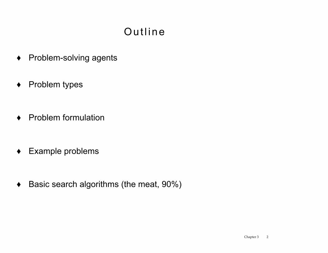
Prob lem-so lv ing agen ts

Simplified form of general agent:

function Simple-Problem-Solving-Agent( percept) returns an action static: seq, an action sequence, initially empty

state, some description of the current world state goal, a goal, initially null problem, a problem formulation

state← Update-State(state,percept) if seqis empty then

goal← Formulate-Goal(state) problem← Formulate-Problem(state,goal) seq← Search( problem)

ac0on← Recommendation(seq,state) seq← Remainder(seq,state) return ac0on

Note: this is offline problem solving; solution executed “eyes closed.” Online problem solving different: uncertainty, incomplete knowledge, etc

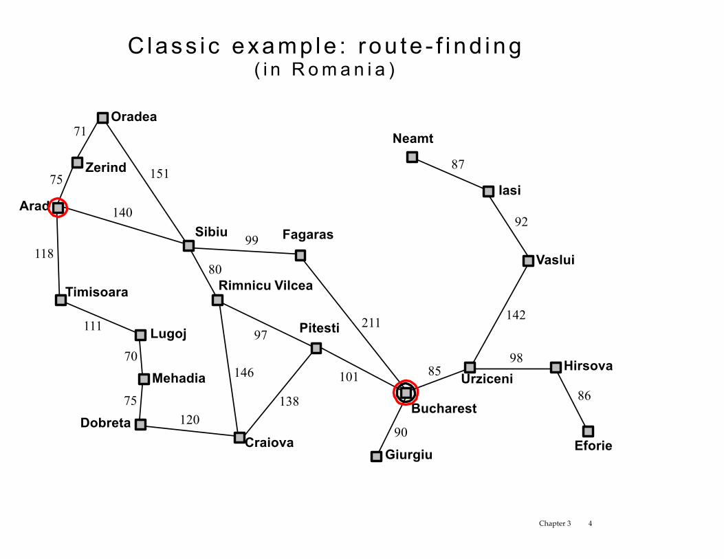
Class i c examp le : rou te - f i nd ing ( i n R o m a n i a )

Urziceni Hirsova

Eforie

Neamt Oradea

Zerind

Arad

Timisoara

Lugoj

Mehadia

Dobreta Craiova

Sibiu Fagaras

Pitesti

Vaslui

Iasi

Bucharest

71

75

118

111

70

75 120

151

140

99

80 Rimnicu Vilcea

97

101

211

138

146 85

90

Giurgiu

98

142

92

87

86

Chapter 3 4

Chapter 3 6

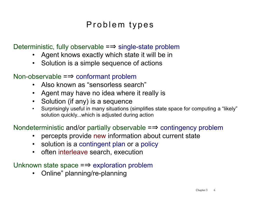
P r o b l e m t ypes

Deterministic, fully observable =⇒ single-state problem •  Agent knows exactly which state it will be in •  Solution is a simple sequence of actions

Non-observable =⇒ conformant problem •  Also known as “sensorless search” •  Agent may have no idea where it really is •  Solution (if any) is a sequence •  Surprisingly useful in many situations (simplifies state space for computing a “likely”

solution quickly...which is adjusted during action

Nondeterministic and/or partially observable =⇒ contingency problem •  percepts provide new information about current state •  solution is a contingent plan or a policy •  often interleave search, execution

Unknown state space =⇒ exploration problem •  Online” planning/re-planning

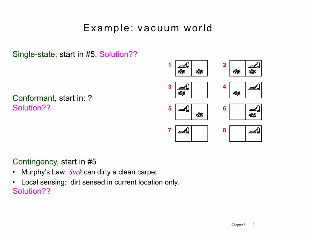
Examp le : v a c u u m wor ld

Single-state, start in #5. Solution??

Conformant, start in: ? Solution??

Contingency, start in #5 •  Murphy’s Law: Suck can dirty a clean carpet •  Local sensing: dirt sensed in current location only. Solution??

1 2

3 4

5 6

7 8

Chapter 3 7

Chapter 3 8

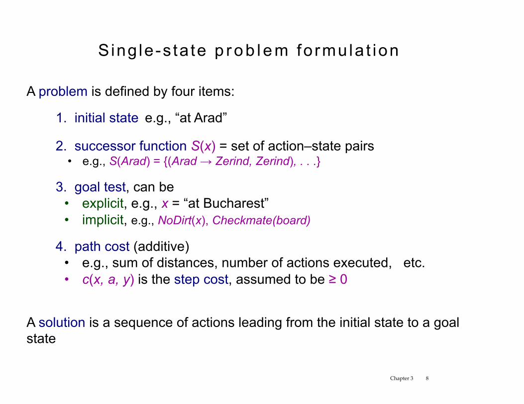
Sing le-s ta te p r o b l e m fo rmu la t ion

A problem is defined by four items:

1. initial state e.g., “at Arad”

2. successor function S(x) = set of action–state pairs •  e.g., S(Arad) = {(Arad → Zerind, Zerind), . . .}

3. goal test, can be •  explicit, e.g., x = “at Bucharest” •  implicit, e.g., NoDirt(x), Checkmate(board)

4. path cost (additive) •  e.g., sum of distances, number of actions executed, etc. •  c(x, a, y) is the step cost, assumed to be ≥ 0

A solution is a sequence of actions leading from the initial state to a goal state

Chapter 3 9

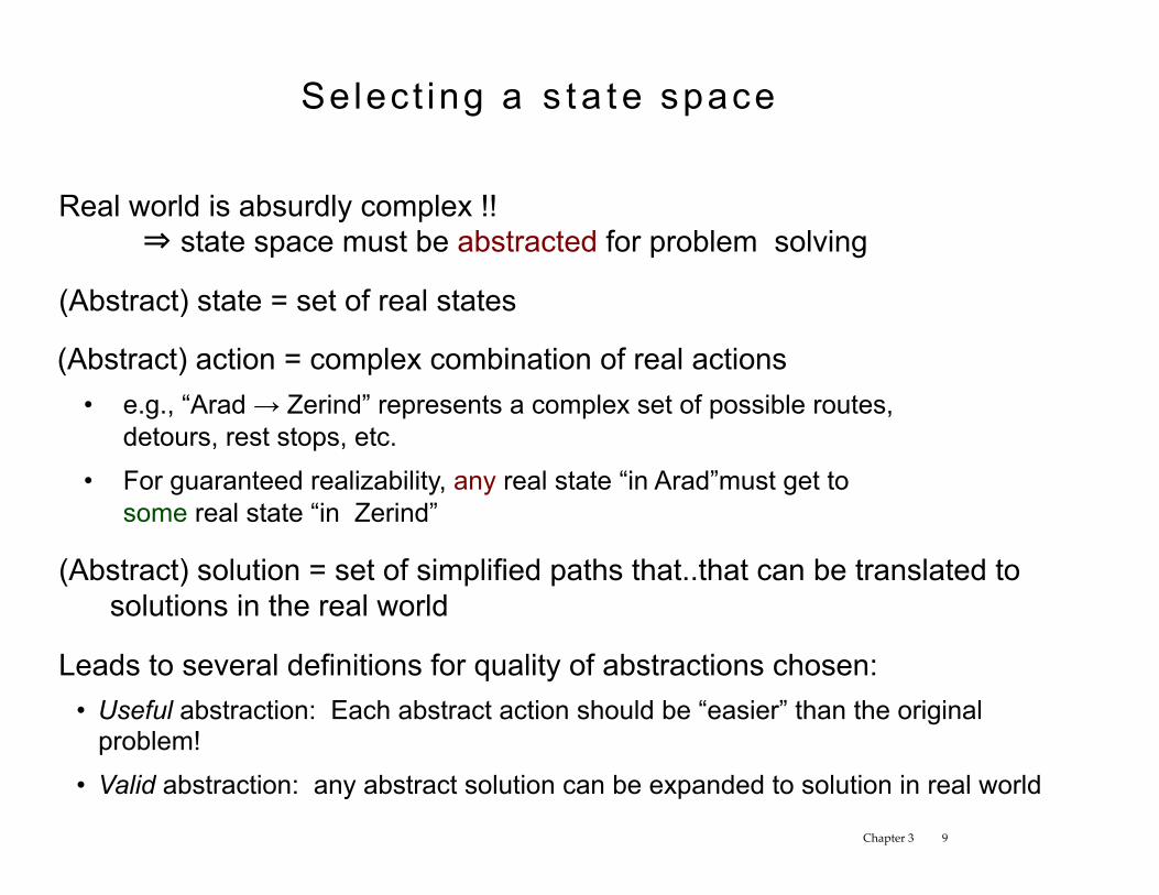
Select ing a s t a te space

Real world is absurdly complex !! ⇒ state space must be abstracted for problem solving

(Abstract) state = set of real states

(Abstract) action = complex combination of real actions •  e.g., “Arad → Zerind” represents a complex set of possible routes,

detours, rest stops, etc. •  For guaranteed realizability, any real state “in Arad”must get to

some real state “in Zerind”

(Abstract) solution = set of simplified paths that..that can be translated to solutions in the real world

Leads to several definitions for quality of abstractions chosen: •  Useful abstraction: Each abstract action should be “easier” than the original

problem!

•  Valid abstraction: any abstract solution can be expanded to solution in real world

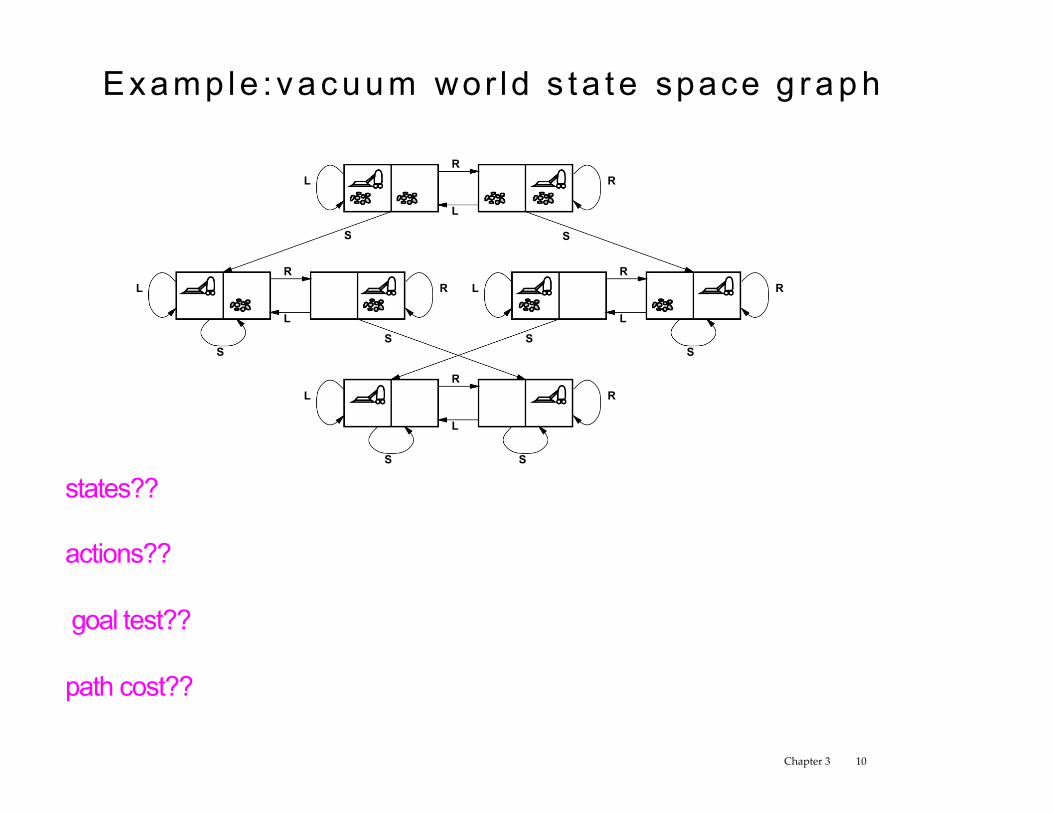
Examp le :v a c u u m wor ld s t a te space g r a p h

R

L

S S

S S

R

L

R

L

R

L

S

S S

S

L

L

L L R

R

R

R

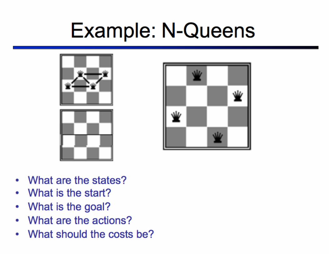
states?? actions?? goal test?? path cost??

Chapter 3 10

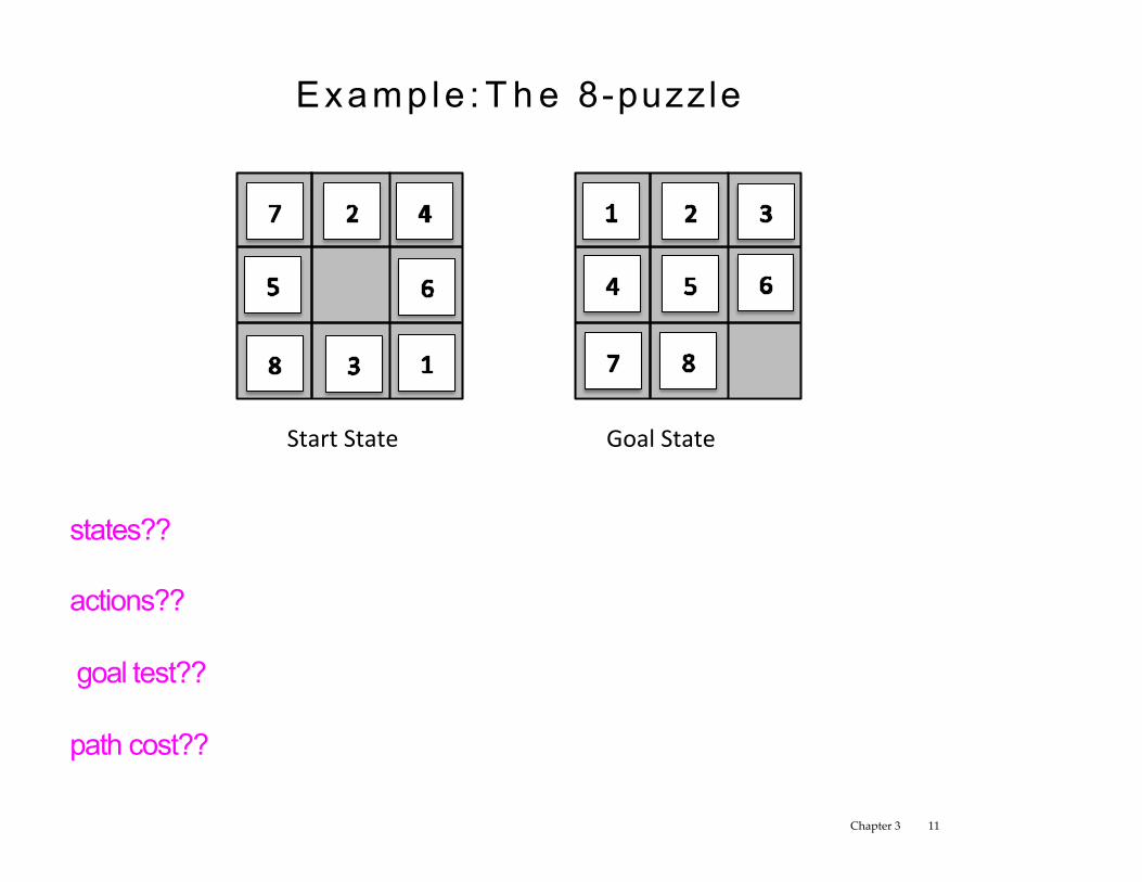
Examp le : T h e 8-puzzle

Chapter 3 11

StartState GoalState

states?? actions?? goal test?? path cost??

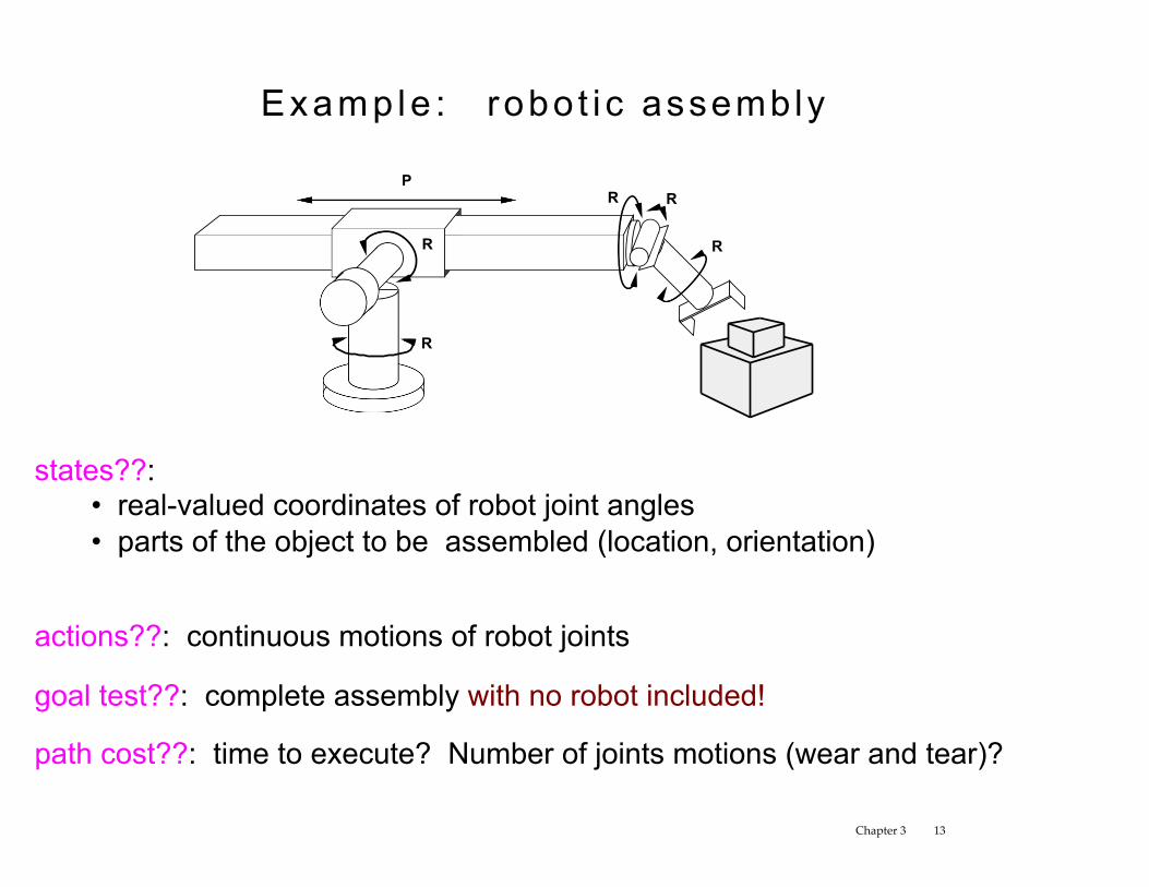
Examp le : robo t i c assembly

R

R R P

R R

states??: •  real-valued coordinates of robot joint angles •  parts of the object to be assembled (location, orientation)

actions??: continuous motions of robot joints

goal test??: complete assembly with no robot included!

path cost??: time to execute? Number of joints motions (wear and tear)?

Chapter 3 13

Chapter 3 14

Tree search a lgo r i thms

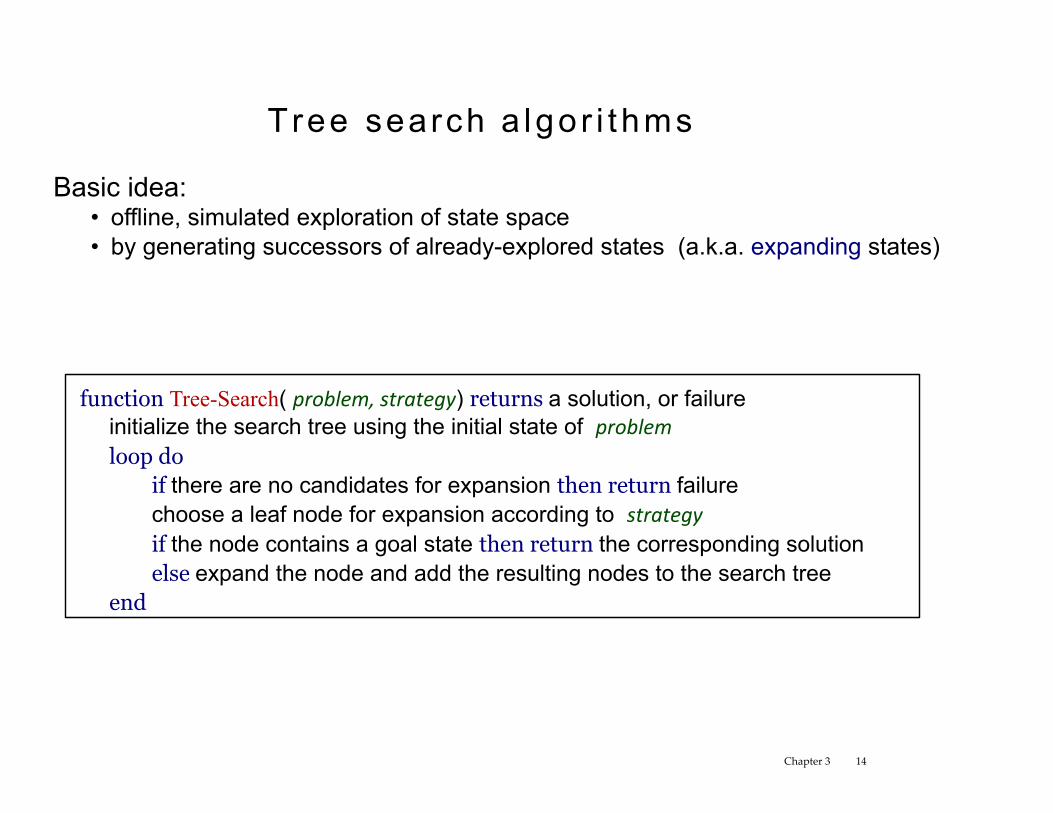
Basic idea: •  offline, simulated exploration of state space •  by generating successors of already-explored states (a.k.a. expanding states)

function Tree-Search( problem,strategy) returns a solution, or failure initialize the search tree using the initial state of problemloop do

if there are no candidates for expansion then return failure choose a leaf node for expansion according to strategyif the node contains a goal state then return the corresponding solution else expand the node and add the resulting nodes to the search tree

end

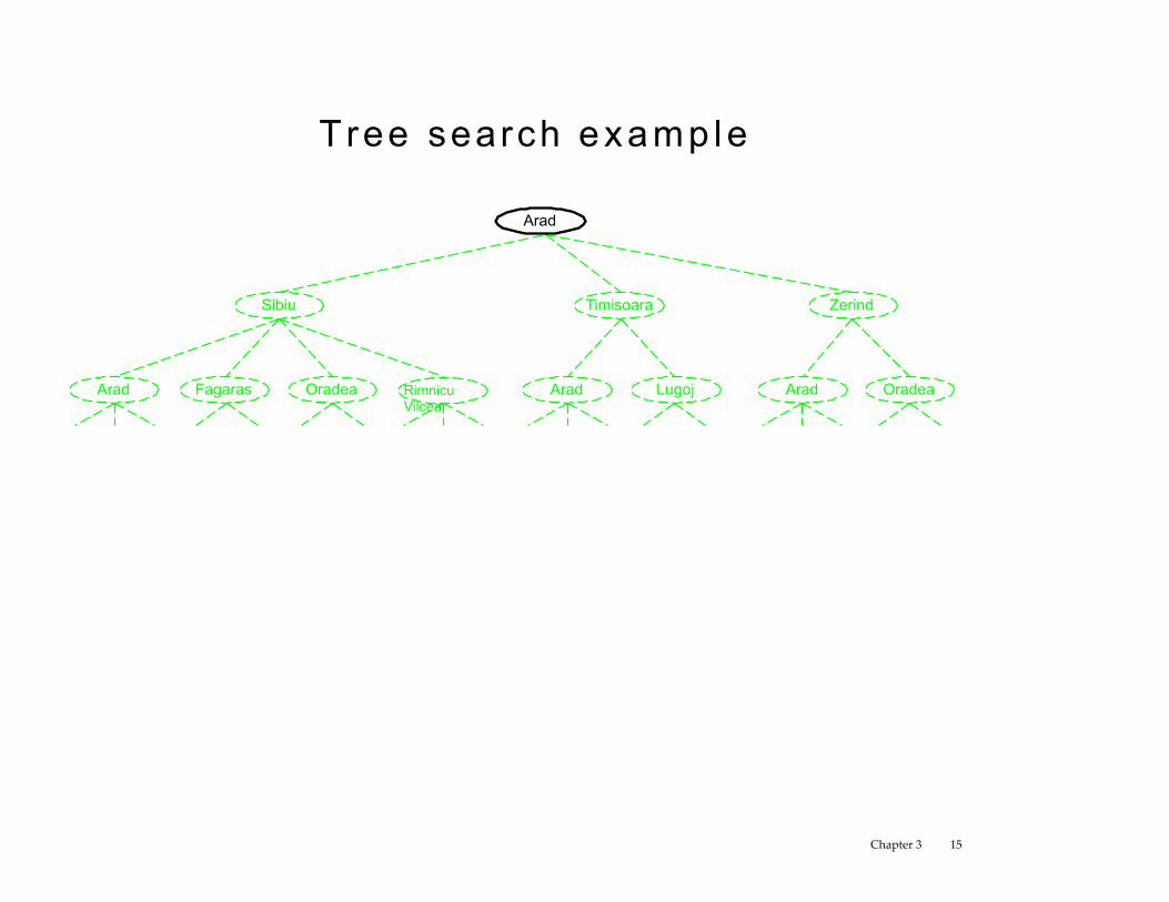
Tree search examp le

Rimnicu Vilcea

Lugoj

Zerind Sibiu

Arad Fagaras Oradea

Timisoara

Arad Arad Oradea

Arad

Chapter 3 15

Concep ts : s ta tes vs. nodes

1

2 3

4 5

6

7

8 1

2 3

4 5

6

7

8

State Node depth = 6

g(x) = 6

state

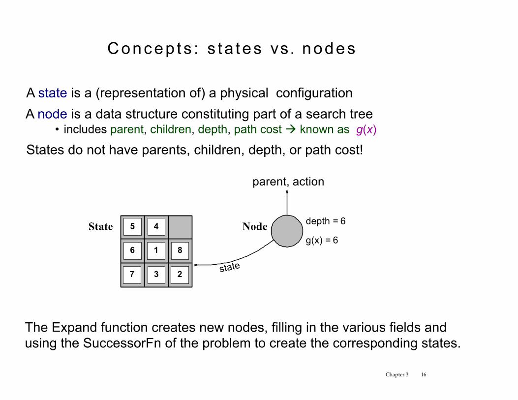
A state is a (representation of) a physical configuration A node is a data structure constituting part of a search tree

•  includes parent, children, depth, path cost à known as g(x)

States do not have parents, children, depth, or path cost!

Chapter 3 16

The Expand function creates new nodes, filling in the various fields and using the SuccessorFn of the problem to create the corresponding states.

parent, action

Imp lemen ta t i on : genera l t r ee search

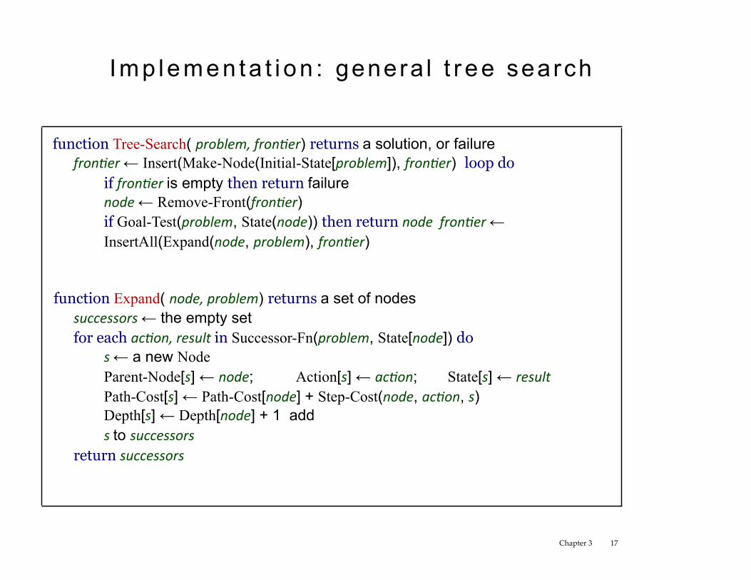
function Tree-Search( problem,fron0er) returns a solution, or failure fron0er← Insert(Make-Node(Initial-State[problem]), fron0er) loop do

if fron0eris empty then return failure node← Remove-Front(fron0er) if Goal-Test(problem, State(node)) then return nodefron0er← InsertAll(Expand(node, problem), fron0er)

function Expand( node,problem) returns a set of nodes

successors← the empty set for each ac0on,resultin Successor-Fn(problem, State[node]) do

s← a new Node Parent-Node[s] ← node; Action[s] ← ac0on; State[s] ← resultPath-Cost[s] ← Path-Cost[node] + Step-Cost(node, ac0on, s) Depth[s] ← Depth[node] + 1 add sto successors

return successors

Chapter 3 17

Chapter 3 18

G r a p h search

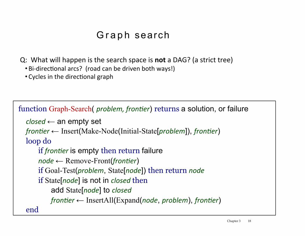
function Graph-Search( problem,fron0er) returns a solution, or failure closed← an empty set fron0er← Insert(Make-Node(Initial-State[problem]), fron0er) loop do

if fron0eris empty then return failure node← Remove-Front(fron0er) if Goal-Test(problem, State[node]) then return nodeif State[node] is not in closedthen

add State[node] to closedfron0er← InsertAll(Expand(node, problem), fron0er)

end

Q:WhatwillhappenisthesearchspaceisnotaDAG?(astricttree)• Bi-direcFonalarcs?(roadcanbedrivenbothways!)• CyclesinthedirecFonalgraph

STOP FOR TODAY!

Chapter 3 20

Search s t ra teg ies

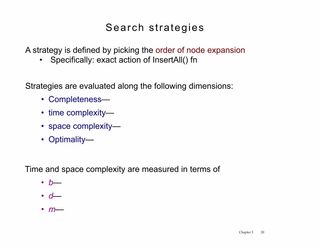
A strategy is defined by picking the order of node expansion •  Specifically: exact action of InsertAll() fn

Strategies are evaluated along the following dimensions: •  Completeness— •  time complexity— •  space complexity— •  Optimality—

Time and space complexity are measured in terms of •  b— •  d— •  m—

Chapter 3 21

Un in fo rmed search s t ra teg ies

Uninformed strategies use only the information available in the problem definition:

•  Breadth-first search

•  Uniform-cost search

•  Depth-first search

•  Depth-limited search

•  Iterative deepening search

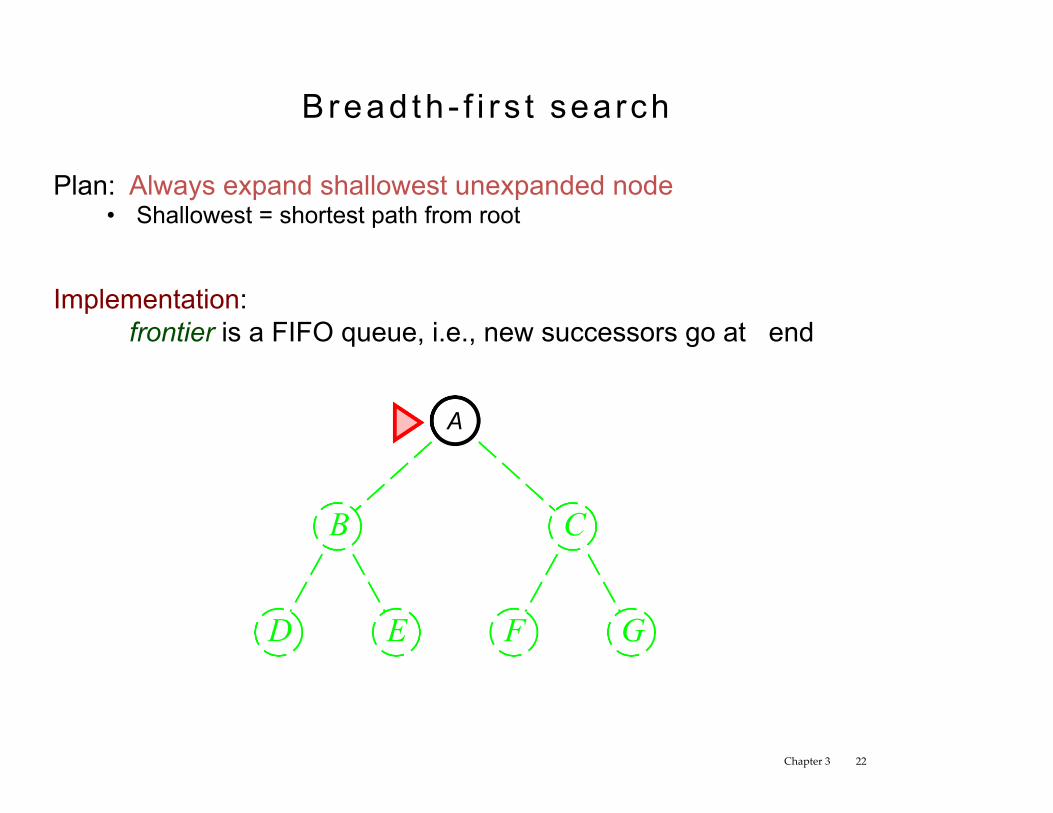
Bread th - f i r s t search

Plan: Always expand shallowest unexpanded node •  Shallowest = shortest path from root

Implementation: frontier is a FIFO queue, i.e., new successors go at end

Chapter 3 22

B C

D E F G

A

P r o p e r t i e s of b read th - f i r s t search

Complete??

Time??

Space??

Optimal??

Chapter 3 23

Uni fo rm-cos t search

Plan: Expand least-cost unexpanded node •  “least cost” = Having the lowest path cost •  Equivalent to breadth-first if step costs all equal

Implementation: frontier = queue ordered by path cost, lowest first

Complete??

Time?? Space?? Optimal??

Chapter 3 24

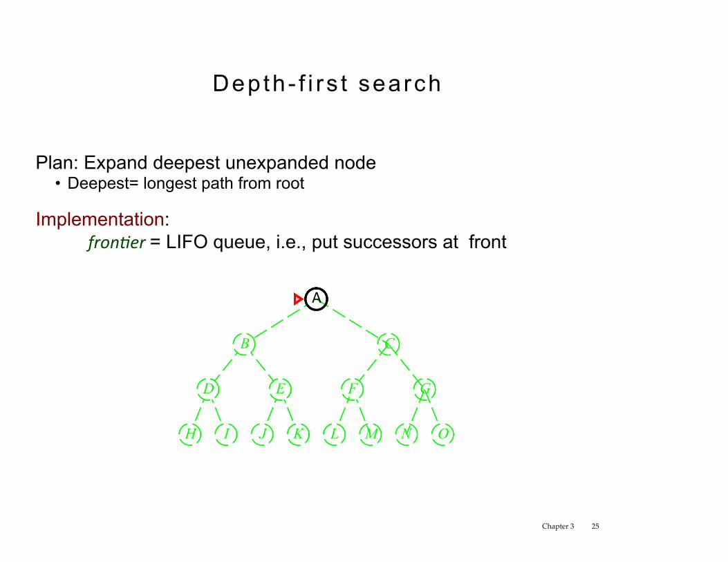
Depth- f i r s t search

Plan: Expand deepest unexpanded node •  Deepest= longest path from root

Implementation: fron0er= LIFO queue, i.e., put successors at front

Chapter 3 25

B C

D E F G

H I J K L M N O

A

P r o p e r t i e s of dep th - f i r s t search

Complete??

Time??

Space??

Optimal??

Chapter 3 26

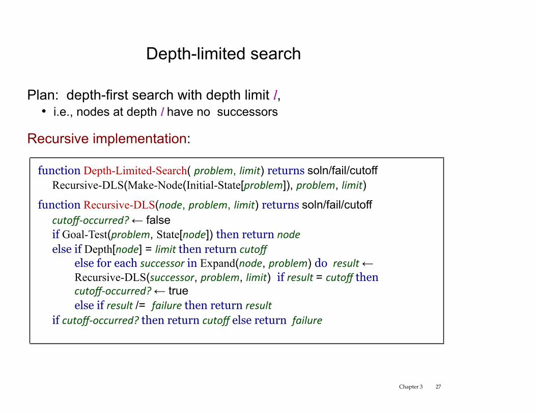
Depth-limited search

Plan: depth-first search with depth limit l, •  i.e., nodes at depth l have no successors

Recursive implementation:

function Depth-Limited-Search( problem, limit) returns soln/fail/cutoff Recursive-DLS(Make-Node(Initial-State[problem]), problem, limit)

function Recursive-DLS(node, problem, limit) returns soln/fail/cutoff cutoff-occurred?← false if Goal-Test(problem, State[node]) then return nodeelse if Depth[node] = limitthen return cutoff

else for each successorin Expand(node, problem) do result← Recursive-DLS(successor, problem, limit) if result= cutoffthen cutoff-occurred?← true else if result/= failurethen return result

if cutoff-occurred?then return cutoffelse return failure

Chapter 3 27

Chapter 3 28

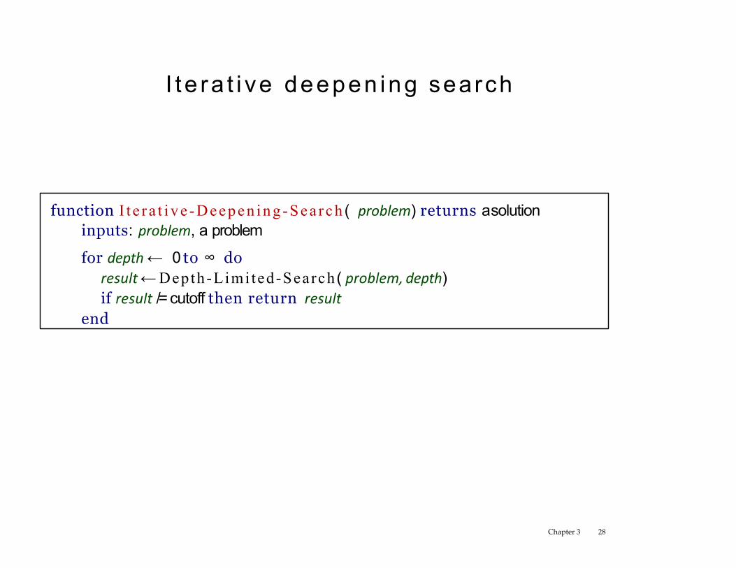
I t e ra t i ve deepen ing search

function I t e r a t i ve -Deepen ing -Sea rch ( problem) returns a solution inputs: problem, a problem

for depth← 0 to ∞ do result← Depth-Limi ted-Search ( problem,depth) if result/= cutoff then return result

end

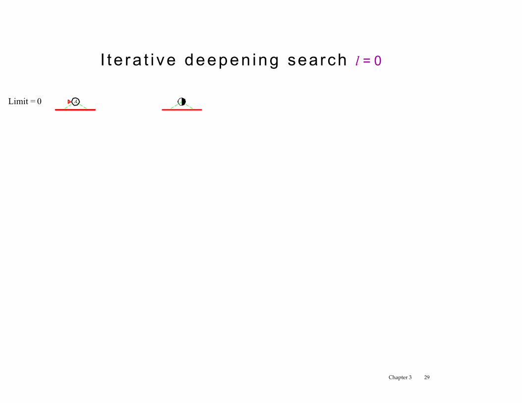
I t e ra t i ve deepen ing search l = 0

Limit = 0 A

Chapter 3 29

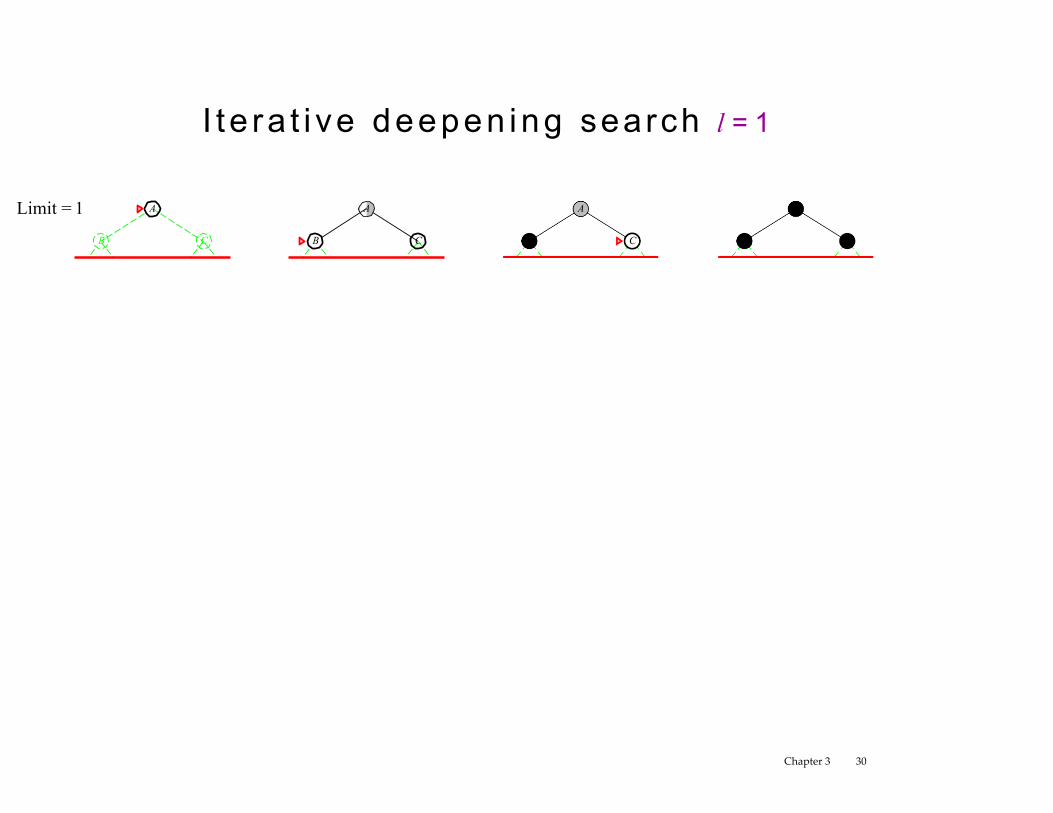
I t e ra t i ve deepen ing search l = 1

Limit = 1 A

B C

A

B C

A

Chapter 3 30

C

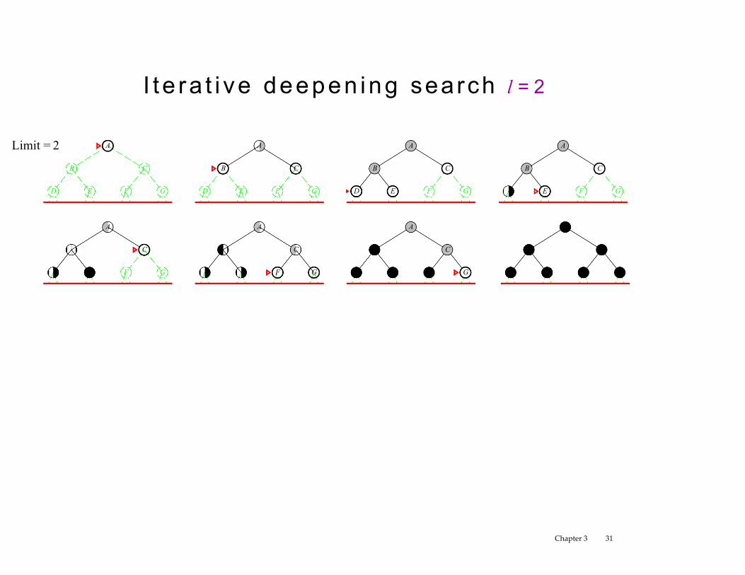
I t e ra t i ve deepen ing search l = 2

Limit = 2 A

Chapter 3 31

B C

D E F G

A

B C

E F G

A

B C

D E F G

A

B C

D E F G

A

C

F G

A

C

G

A

C

F G

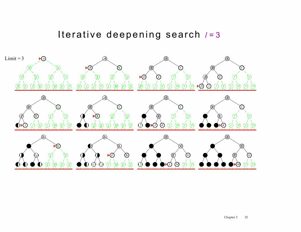
I t e ra t i ve deepen ing search l = 3

Limit = 3

A

C

F G

M N O

A

C

F G

L M N O

A

C

F G

L M N O

A

C

F G

L M N O

A

B C

E F G

K L M N O

A

B C

E F G

J K L M N O

A

B C

E F G

J K L M N O

A

B C

D E F G

I J K L M N O

A

B C

D E F G

H I J K L M N O

A

B C

D E F G

H I J K L M N O

A

B C

D E F G

H J K L M N O I

A

Chapter 3 32

B C

D E F G

H I J K L M N O

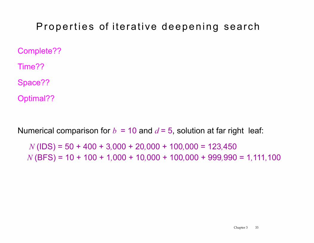
P r o p e r t i e s of i te ra t i ve deepen ing search

Complete??

Time??

Space??

Optimal??

Numerical comparison for b = 10 and d = 5, solution at far right leaf:

N (IDS) = 50 + 400 + 3,000 + 20,000 + 100,000 = 123,450 N (BFS) = 10 + 100 + 1,000 + 10,000 + 100,000 + 999,990 = 1,111,100

Chapter 3 33

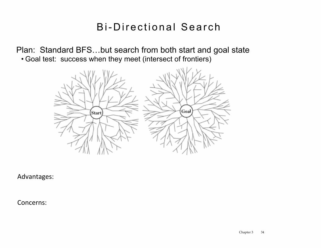
B i - D i r e c t i o n a l S e a r c h

Plan: Standard BFS…but search from both start and goal state • Goal test: success when they meet (intersect of frontiers)

Chapter 3 34

Advantages:

Concerns:

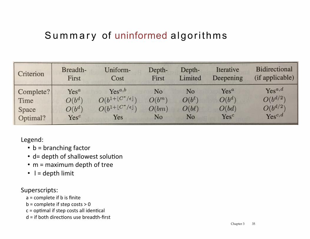
S u m m a r y of uninformed a lgo r i thms

Chapter 3 35

Legend:•  b=branchingfactor•  d=depthofshallowestsoluFon•  m=maximumdepthoftree•  l=depthlimit

Superscripts:a=completeifbisfiniteb=completeifstepcosts>0c=opFmalifstepcostsallidenFcald=ifbothdirecFonsusebreadth-first