Problem Solving and Search in Artificial Intelligence

Local Search, Stochastic Hill Climbing, Simulated Annealing

Nysret MusliuDatabase and Artificial Intelligence GroupInstitut für Informationssysteme, TU-Wien

Local Search1. Pick a solution from the search space and evaluate

its merit. Define this as current solution2. Apply a transformation to the current solution to

generate a new solution and evaluate its merit3. If the new solution is better than the current

solution then exchange it with the current solution 4. Repeat steps 2 and three until no transformation in

the given set improves the current solution

Local search for SATGSAT algorithm is based on flip of variable that results in the largest decrease number of unsatisfied clauses

Procedure GSATbegin

for i=1 step 1 until MAX-TRIES dobegin

T<- a randomly generated truth assignmentfor j=1 step 1 until MAX-FLIPS do

if T satisfies the formula then return(T)else make a flip of variable in T that results in the

largest decrease in the number of unsatisfied clauses endreturn(“no satisfying assignment found“)

end

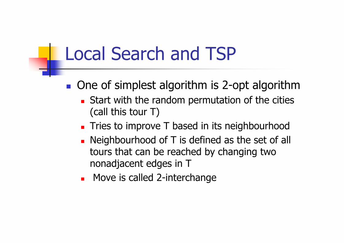
Local Search and TSP

One of simplest algorithm is 2-opt algorithmStart with the random permutation of the cities (call this tour T)Tries to improve T based in its neighbourhoodNeighbourhood of T is defined as the set of all tours that can be reached by changing two nonadjacent edges in TMove is called 2-interchange

Local Search and TSP2-interchange move

2-Opt Algorithm

A new tour T‘after the 2-interchange move replaces T if it is betterIf non of the tours in neighbourhood is better than the tour T the algorithm terminatesThe algorithm should be started from several random permutations2-opt algorithm can be extended to k-opt algorithm

Lin-Kernighan Algorithm

Refines the k-opt strategy by allowing k to vary from one iteration to anotherIt favors the largest improvement in neighbourhood, not the first improvement like in k-opt Generates near optimal solutions for TSPswith up to million citiesNeeds under one hour on a modern workstation

Greedy Algorithms

Simple algorithmsAssigns the values for all decisions variables one by one and at every step makes the best available decisionHeuristic provides the best possible move at each stepDo not always return the optimum solution

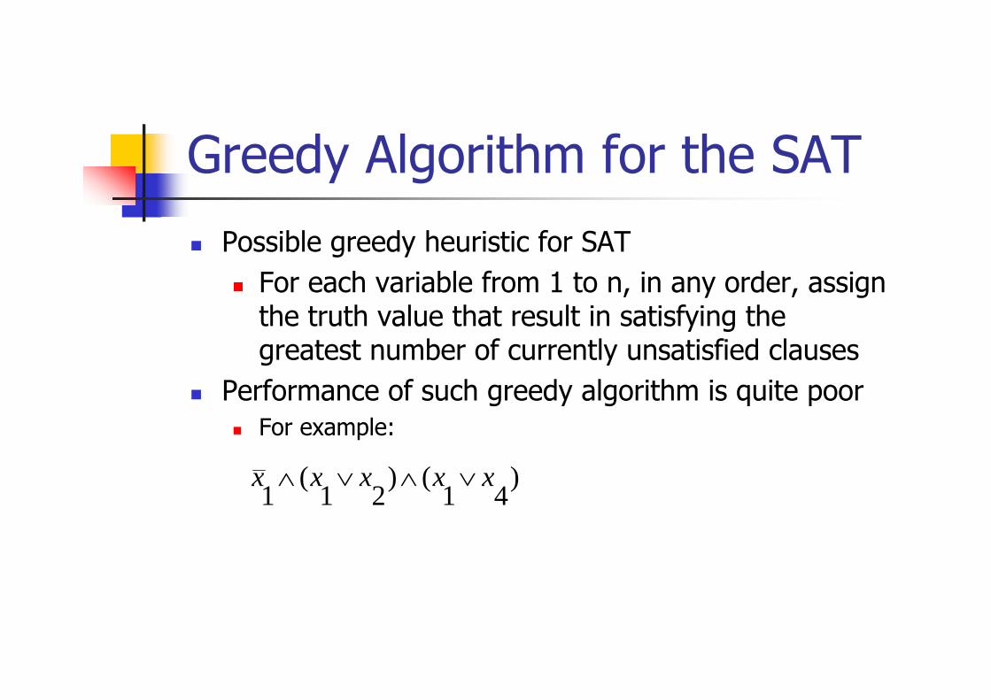
Greedy Algorithm for the SATPossible greedy heuristic for SAT

For each variable from 1 to n, in any order, assign the truth value that result in satisfying the greatest number of currently unsatisfied clauses

Performance of such greedy algorithm is quite poorFor example:

)41

()21

(1

xxxxx ∨∧∨∧

Greedy Algorithm for the SAT

Possible improve of previous greedy algorithm

Sort all variables on basis of their frequency, from the smallest to the largestFor each variable in order, assign a value that would satisfy the greatest number of currently unsatisfied clauses

Further improves to the greedy algorithm can be doneThere is no good greedy algorithm for the SAT

Greedy Algorithm for the TSP

Nearest neighbourhood heuristicStart from random cityProceed to the nearest unvisited cityContinue with step 2 until every city has been visited

The tour with this algorithms can be far from perfect

Greedy Algorithm for the TSPFor example with this heuristic if we start from A the following tour will be generated: A-B-C-D-A (cost=33)There exist much better tour A-C-B-D-A (cost=19)

D

A C

B

5

4

2

3

7

23

Local search

+: Ease of implementation+: Guarantee of local optimality usually in small computational time+: No need for exact model of the problem-: Poor quality of solution due to getting stuck in poor local optima

Modern Heuristics (Metaheuristics)

These algorithms guide an underlying heuristic/local search to escape from being trapped in a local optima and to explore better areas of the solution spaceExamples:

Single solution approaches: Simulated Annealing, TabuSearch, etc.Population based approaches: Genetic algorithm, Memeticalgorithm, ACO, etc.

+: Able to cope with inaccuracies of data and model, large sizes of the problem and real-time problem solving+: Including mechanisms to escape from local optima of their embedded local search algorithms+: Ease of implementation+: No need for exact model of the problem-: Usually no guarantee of optimality

Elements of Local Search•Representation of the solution

• Evaluation function

• Neighbourhood function: to define solutions which can be considered close to a given solution. For example:

• For optimisation of real-valued functions in elementary calculus, for a current solution x0, neighbourhood is defined as an interval (x0 –r, x0+r)

• In clustering problem, all the solutions which can be derived from a given solution by moving one customer from one cluster to another

Elements of Local SearchThe larger the neighbourhood, the harder it is to explore and the better the quality of its local optimumFinding an efficient neighbourhood:

balance between the quality of the solution and the complexity of the search

Neighbourhood search strategyrandomsystematic search

Acceptance criterion: first improvementbest improvement, best of non-improving solutions, random criteria

Hill Climbing Algorithm

1. Pick a random point in the search space2. Consider all the neighbours of the current state3. Choose the neighbour with the best quality and

move to that state4. Repeat 2 through 4 until all the neighbouring

states are of lower quality5. Return the current state as the solution state

The Problem with Hill ClimbingGets stuck at local minimaPossible solutions:

Try several runs, starting at different positions

Increase the size of the neighbourhood (e.g. in TSP try 3-opt rather than 2-opt)

Stochastic Hill-ClimbingOnly one solution from neighbourhood is selectedThis solution will be accepted for the next iteration

with some probability, which depends from the difference between current solution and selected solution

Stochastic Hill-ClimbingProcedure stochastic hill-climberbegin

t=0select a current string vc at randomevaluate vc

repeatselect the string vn from the neighborhood of vc

select vn with probabilityt=t+1until t=MAX

end

T)eval(v)eval(v nc

e−

+1

1

Stochastic Hill Climbing

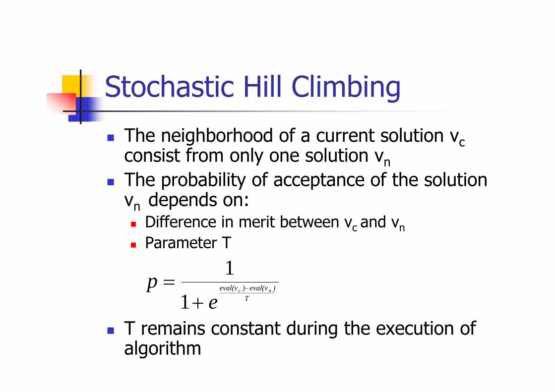
The neighborhood of a current solution vcconsist from only one solution vn

The probability of acceptance of the solution vn depends on:

Difference in merit between vc and vn

Parameter T

T remains constant during the execution of algorithm

T)eval(v)eval(v nc

ep −

+=

11

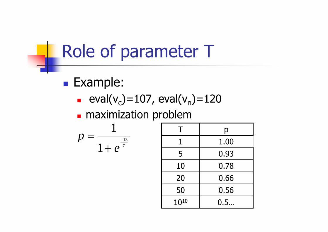
Role of parameter T

Example:eval(vc)=107, eval(vn)=120maximization problem

Tep 13

11

−

+=

0.5…1010

0.5650

0.6620

0.7810

0.935

1.001

pT

Role of parameter T

Example:eval(vc)=107, eval(vn)=120Maximization problem

Tep 13

11

−

+=

0.5…1010

0.5650

0.6620

0.7810

0.935

1.001

pT

The greater the parameter T, the smaller the importance of the relative merit of the competing points vc and vn

Role of parameter T

If T is huge -> search becomes randomT is very small -> stochastic hill-climber reverts into ordinary hill climber

Tep 13

11

−

+=

0.5…1010

0.5650

0.6620

0.7810

0.935

1.001

pT

The greater the parameter T, the smaller the importance of the relative merit of the competing points vc and vn

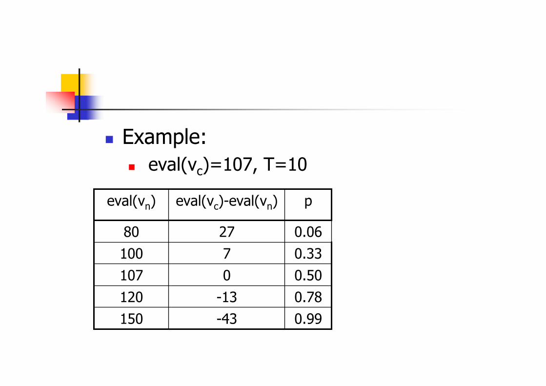
Example:eval(vc)=107, T=10

15012010710080

eval(vn)

-43-130727

eval(vc)-eval(vn)

0.990.780.500.330.06

p

Example:eval(vc)=107, T=10

15012010710080

eval(vn)

-43-130727

eval(vc)-eval(vn)

0.990.780.500.330.06

pIf eval(vc)=eval(vn), the probability of acceptance is 0.5

Simulated Annealing

Changes the parameter T during the searchStarts with high value for T – random search The value of T gradually decreasesTo the end T is very small and the SA behaves like an ordinary Hill-climber

Simulated Annealing

Is based on the analogy from the thermodynamicsTo grow a crystal, the row material is heated to a molten stateThe temperature of the crystal melt is reduced until the crystal structure is frozen inCooling should not be done two quickly, otherwise some irregularities are locked in the crystal structure

Simulated AnnealingProzedure simulated annealingbegin

t=0Intialize Tselect a current string vc at randomevaluate vcrepeatrepeat

select a new point vn in the neighborhood of vc

if eval(vc) < eval(vn) then vc =vn

else if then vc=vnuntil (termination-condition)T=g(T,t)t=t+1until (halting-criterion)

end

T)ceval(v)neval(v

erandom−

<)1,0[

SA – problem specific questions

What is a solution?What are the neighbors of a solution?What is a cost of a solutionHow do we determine the initial solution

SA – specific questions

How do we determine the intial“temperature” T”How do we determine the cooling ration g(T,t)?How do we determine the termination condition?How do we determine the halting criterion?

STEP 1: T=Tmaxselect vc at random

STEP 2: pick a point vn from the neighborhood of vc

if eval(vn) is better than the val(vc)then select it (vc=vn)else select it with probability

repeat this step kT times

STEP 3: set T=rTif

then goto STEP 2else goto STEP 1

Teval

eΔ−

minTT ≥

Simulated Annealing for SAT problemProcedure SA-SATbegin

tries=0repeat

v <- random truth assignmentj=0repeat

If v satisfies the clauses then return v

for k=1 to the number of variables do begin

compute the increase (decreases) δ in the number of clauses made true if vk was flippedflip variable vk with the probabilityv <- new assignment if the flip is made

endj=j+1

untiltries=tries+1

until tries=MAX-TRIESend

jreTT −=max

1)1( −−

+ Teδ

minTT ≤

SA for SAT

r represents a decay rate for the temperatureSpears (1996) used

Tmax=0.03 and Tmin=0.01 r depend on the number of variables and number of tries

SA-SAT appeared to satisfy at least as many formulas as GSAT, with less workAdvantage of SA-SAT came from its backward moves

Other application of SA

Traveling Salesman ProblemVLSI designProduction schedulingTimetabling problemsImage processing…

ReferencesZ. Michalewicz and D. B. Fogel. How to Solve It: Modern Heuristics

Chapters 3 (sec. 3.2), 4 (sec. 4.1) , 5 (sec. 5.1)

Other papersSimulated annealing for hard satisfiability problems : W.M. Spears

Optimization by Simulated Annealing: An Experimental Evaluation; Part I, Graph PartitioningDS Johnson, CR Aragon, LA McGeoch, C Schevon