Problem set 2 - Welcome to the Chair in Macroeconomics! 1 Problem 1 (differential equations) 2 Problem 2 (the Solow growth model in discrete time) 3 Problem 3 (the CES production function)

Problem set 2Long run macroeconomic growth

Markus Roth

Chair for MacroeconomicsJohannes Gutenberg Universität Mainz

December 3, 2010

Markus Roth (Advanced Macroeconomics) Problem set 2 December 3, 2010 1 / 38

Contents

1 Problem 1 (differential equations)

2 Problem 2 (the Solow growth model in discrete time)

3 Problem 3 (the CES production function)


Problem 1 (differential equations)

Contents






Differential equations

• In this problem we only consider linear differential equations.

• Unlike nonlinear differential equations, we are able to solve themanalytically.

• In addition we focus on the simplified case where the coefficientsare constant.

• Consider the following homogenous linear differential equation

xt = axt.

• The term “homogenous” indicates that this differential equation isa special case of

xt = axt + b

where b = 0.



Homogenous differential equation

• We can rewrite the equation as follows

xtxt

= a.

• From this representation we find that a is the growth rate of thevariable xt in continuous time.

• For interpretation as a growth rate think of the left hand side as

xtxt

= lim∆→0

xt+∆ − xtxt

.

• The solution to this differential equation is

xt = eatx0,

where x0 is some initial condition of xt which is known.

• We can easily verify that this is indeed the solution by taking thefirst derivative with respect to time.



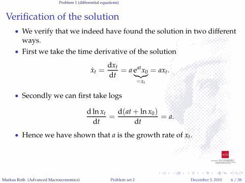
Verification of the solution

• We verify that we indeed have found the solution in two differentways.

• First we take the time derivative of the solution

xt =dxtdt

= a eatx0︸︷︷︸

=xt

= axt.

• Secondly we can first take logs

d ln xtdt

=d(at+ ln x0)

dt= a.

• Hence we have shown that a is the growth rate of xt.



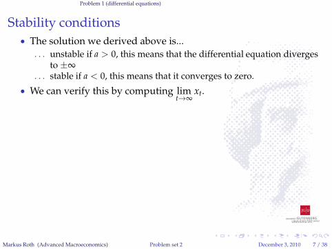
Stability conditions

• The solution we derived above is...

. . . unstable if a > 0, this means that the differential equation divergesto ±∞

. . . stable if a < 0, this means that it converges to zero.

• We can verify this by computing limt→∞

xt.



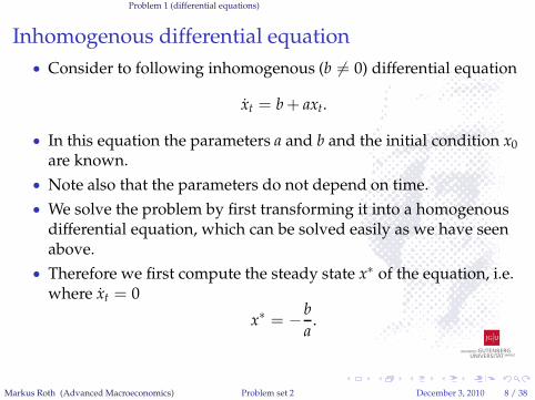
Inhomogenous differential equation

• Consider to following inhomogenous (b 6= 0) differential equation

xt = b+ axt.

• In this equation the parameters a and b and the initial condition x0are known.

• Note also that the parameters do not depend on time.

• We solve the problem by first transforming it into a homogenousdifferential equation, which can be solved easily as we have seenabove.

• Therefore we first compute the steady state x∗ of the equation, i.e.where xt = 0

x∗ = −b

a.



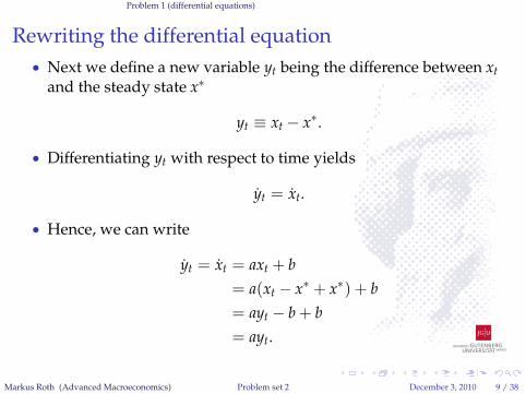
Rewriting the differential equation

• Next we define a new variable yt being the difference between xtand the steady state x∗

yt ≡ xt − x∗.

• Differentiating yt with respect to time yields

yt = xt.

• Hence, we can write

yt = xt = axt + b

= a(xt − x∗ + x∗) + b

= ayt − b+ b

= ayt.



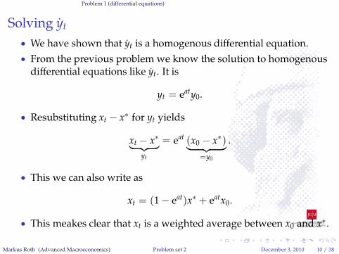
Solving yt• We have shown that yt is a homogenous differential equation.

• From the previous problem we know the solution to homogenousdifferential equations like yt. It is

yt = eaty0.

• Resubstituting xt − x∗ for yt yields

xt − x∗︸︷︷︸

yt

= eat (x0 − x∗)︸︷︷︸

=y0

.

• This we can also write as

xt = (1− eat)x∗ + eatx0.

• This meakes clear that xt is a weighted average between x0 and x∗.



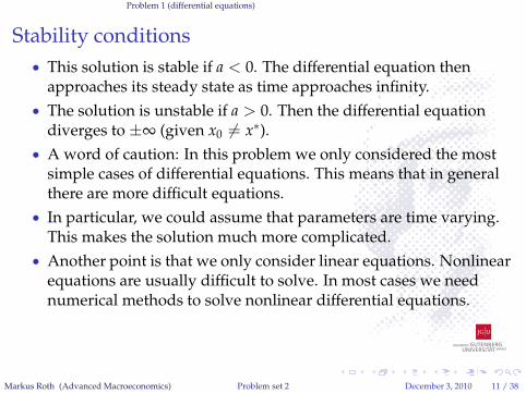
Stability conditions

• This solution is stable if a < 0. The differential equation thenapproaches its steady state as time approaches infinity.

• The solution is unstable if a > 0. Then the differential equationdiverges to ±∞ (given x0 6= x∗).

• A word of caution: In this problem we only considered the mostsimple cases of differential equations. This means that in generalthere are more difficult equations.

• In particular, we could assume that parameters are time varying.This makes the solution much more complicated.

• Another point is that we only consider linear equations. Nonlinearequations are usually difficult to solve. In most cases we neednumerical methods to solve nonlinear differential equations.


Problem 2 (the Solow growth model in discrete time)

Contents






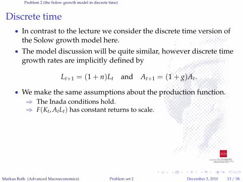
Discrete time

• In contrast to the lecture we consider the discrete time version ofthe Solow growth model here.

• The model discussion will be quite similar, however discrete timegrowth rates are implicitly defined by

Lt+1 = (1+ n)Lt and At+1 = (1+ g)At.

• We make the same assumptions about the production function.

⇒ The Inada conditions hold.⇒ F(Kt,AtLt) has constant returns to scale.



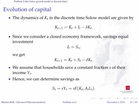
Evolution of capital

• The dynamics of Kt in the discrete time Solow model are given by

Kt+1 = Kt + It − δKt.

• Since we consider a closed economy framework, savings equalinvestment

It = St,

we getKt+1 = Kt + St − δKt.

• We assume that households save a constant fraction s of theirincome Yt.

• Hence, we can determine savings as

St = sYt = sF(Kt,AtLt).



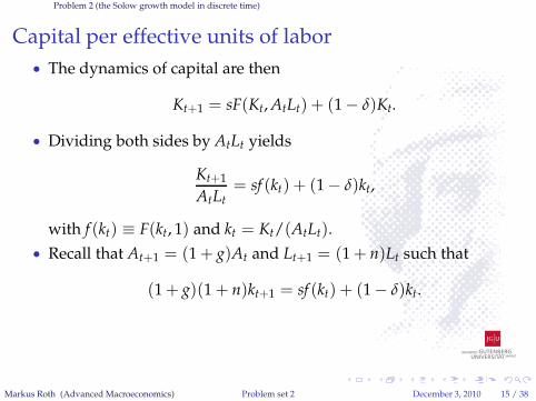
Capital per effective units of labor

• The dynamics of capital are then

Kt+1 = sF(Kt,AtLt) + (1− δ)Kt.

• Dividing both sides by AtLt yields

Kt+1

AtLt= sf (kt) + (1− δ)kt,

with f (kt) ≡ F(kt, 1) and kt = Kt/(AtLt).

• Recall that At+1 = (1+ g)At and Lt+1 = (1+ n)Lt such that

(1+ g)(1+ n)kt+1 = sf (kt) + (1− δ)kt.



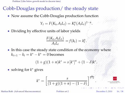
Cobb-Douglas production/ the steady state

• Now assume the Cobb-Douglas production function

Yt = F(Kt,AtLt) = Kαt (AtLt)

1−α.

• Dividing by effective units of labor yields

F(Kt,AtLt)

AtLt= f (kt) = kα

t .

• In this case the steady state condition of the economy wherekt+1 − kt = k∗ − k∗ = 0 becomes

(1+ g)(1+ n)k∗ = s [k∗]α + (1− δ)k∗.

• solving for k∗ gives

k∗ =

[s

(1+ g)(1+ n)− (1− δ)

] 11−α

.



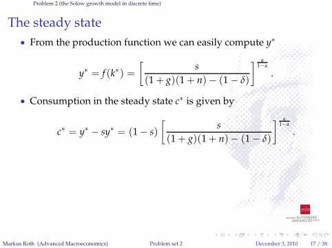
The steady state

• From the production function we can easily compute y∗

y∗ = f (k∗) =

[s

(1+ g)(1+ n)− (1− δ)

] α

1−α

.

• Consumption in the steady state c∗ is given by

c∗ = y∗ − sy∗ = (1− s)

[s

(1+ g)(1+ n)− (1− δ)

] α

1−α

.



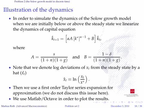
Illustration of the dynamics

• In order to simulate the dynamics of the Solow growth modelwhen we are initially below or above the steady state we linearizethe dynamics of capital equation

kt+1 =[

αA [k∗]α−1 + B]

kt,

where

A =s

(1+ n)(1+ g)and B =

1− δ

(1+ n)(1+ g).

• Note that we denote log deviations of xt from the steady state by ahat (xt)

xt ≡ ln( xtx∗

)

.

• Then we use a first order Taylor series expansion forapproximation (we do not discuss this issue here).

• We use Matlab/Octave in order to plot the results.



-0.5

-0.4

-0.3

-0.2

-0.1

0

0 20 40 60 80 100

khat

Time

khat

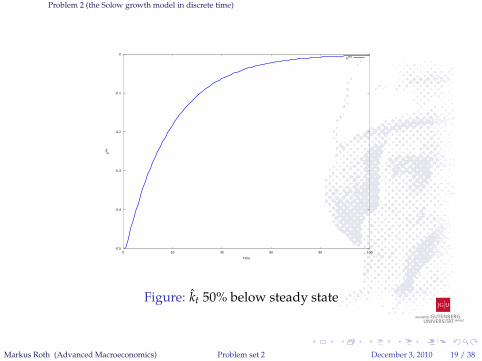
Figure: kt 50% below steady state



0

0.1

0.2

0.3

0.4

0.5

0 20 40 60 80 100

khat

Time

khat

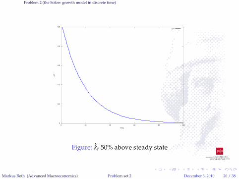
Figure: kt 50% above steady state



-0.8

-0.6

-0.4

-0.2

0

0.2

0.4

0.6

0.8

0 20 40 60 80 100

khat

Time

khatlow

khathigh

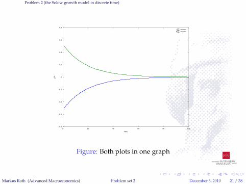
Figure: Both plots in one graph



The golden rule level savings rate s∗

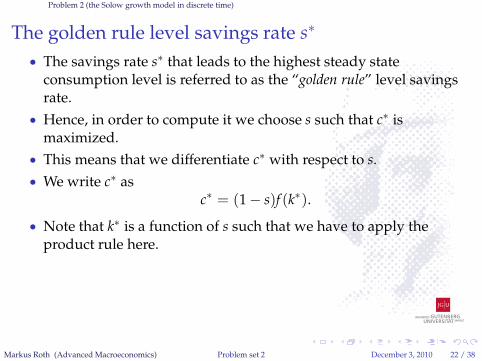
• The savings rate s∗ that leads to the highest steady stateconsumption level is referred to as the “golden rule” level savingsrate.

• Hence, in order to compute it we choose s such that c∗ ismaximized.

• This means that we differentiate c∗ with respect to s.

• We write c∗ asc∗ = (1− s)f (k∗).

• Note that k∗ is a function of s such that we have to apply theproduct rule here.



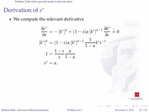
Derivation of s∗

• We compute the relevant derivative

∂c∗

∂s= − [k∗]α + (1− s)α [k∗]α−1 ∂k∗

∂s

!= 0

[k∗]α = (1− s)α [k∗]α−1 1

1− αk∗s−1

1 =1− s

s

α

1− α

s∗ = α.


Problem 3 (the CES production function)

Contents






The CES production function

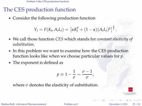
• Consider the following production function

Yt = F(Kt,AtLt) =[αK

pt + (1− α)(AtLt)

p] 1p .

• We call those function CESwhich stands for constant elasticity ofsubstitution.

• In this problem we want to examine how the CES productionfunction looks like when we choose particular values for p.

• The exponent is defined as

p ≡ 1−1

σ=

σ − 1

σ,

where σ denotes the elasticity of substitution.



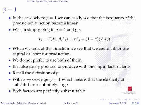
p = 1

• In the case where p = 1 we can easily see that the isoquants of theproduction function become linear.

• We can simply plug in p = 1 and get

Yt = F(Kt,AtLt) = αKt + (1− α)(AtLt).

• When we look at this function we see that we could either usecapital or labor for production.

• We do not prefer to use both of them.

• It is also easily possible to produce with one input factor alone.

• Recall the definition of p.

• With σ → ∞ we get p = 1 which means that the elasticity ofsubstitution is infinitely large.

• Both factors are perfectly substitutable.



0

1

2

3

4

5

0

1

2

3

4

50

1

2

3

4

5

F(K,L)

K

L

F(K,L)

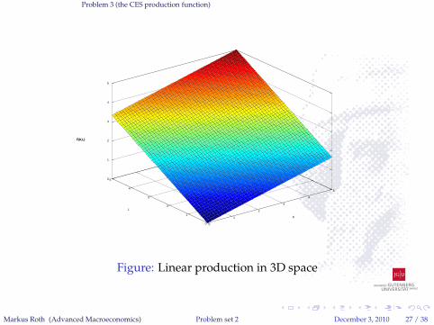
Figure: Linear production in 3D space



0

1

2

3

4

5

0 1 2 3 4 5

L

K

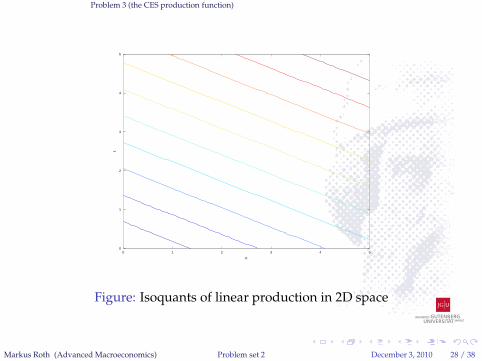
Figure: Isoquants of linear production in 2D space



p → 0

• The analysis for p → 0 is more complicated.

• We cannot set p = 0, hence we need another method to computethe resulting production function.

• We rewrite the function in logarithms first

lnYt =ln

[αK

pt + (1− α)(AtLt)p

]

p.

• Then we compute the limit limp→0 and we recognize that thenominator and the denominator approach zero.

• Since nominator and denominator approach zero we are able touse the rule of L‘Hospital.

• This rule says that provided the limit of the nominator anddenominator separately tend to zero we can compute the limit ofthe function by computing the limit of the derivatives ofnominator and denominator.



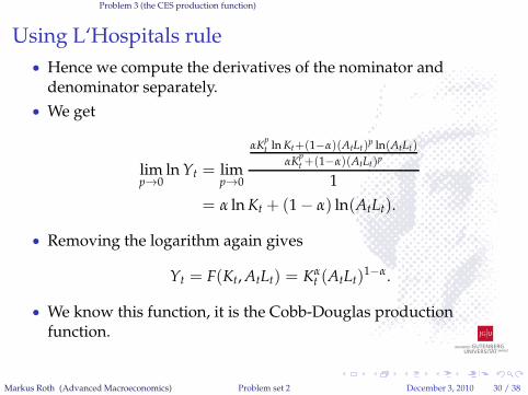
Using L‘Hospitals rule

• Hence we compute the derivatives of the nominator anddenominator separately.

• We get

limp→0

lnYt = limp→0

αKpt lnKt+(1−α)(AtLt)

p ln(AtLt)

αKpt +(1−α)(AtLt)p

1

= α lnKt + (1− α) ln(AtLt).

• Removing the logarithm again gives

Yt = F(Kt,AtLt) = Kαt (AtLt)

1−α.

• We know this function, it is the Cobb-Douglas productionfunction.



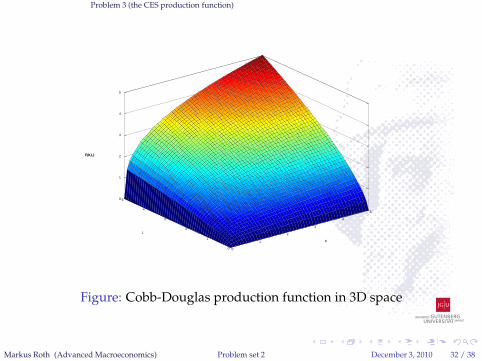
Cobb-Douglas production

• Different to the linear case before we prefer to use bothproduction inputs.

• However we can use more of one and less of the other input.

• Hence, both factor inputs are substitutable but to an intermediateextent.


• With p → 0 we have σ → 1 which means that the elasticity ofsubstitution is equal to one.



0

1

2

3

4

5

0

1

2

3

4

50

1

2

3

4

5

F(K,L)

K

L

F(K,L)

Figure: Cobb-Douglas production function in 3D space



0

1

2

3

4

5

0 1 2 3 4 5

L

K

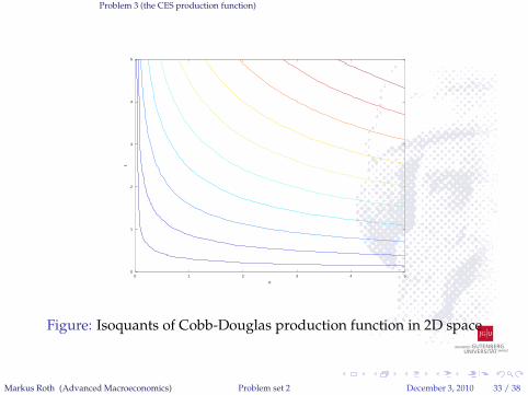
Figure: Isoquants of Cobb-Douglas production function in 2D space



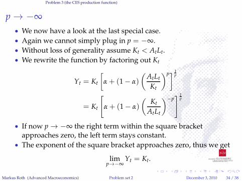
p → −∞

• We now have a look at the last special case.

• Again we cannot simply plug in p = −∞.

• Without loss of generality assume Kt < AtLt.

• We rewrite the function by factoring out Kt

Yt = Kt

[

α + (1− α)

(AtLtKt

)p]1p

= Kt

[

α + (1− α)

(Kt

AtLt

)−p] 1

p

• If now p → −∞ the right term within the square bracketapproaches zero, the left term stays constant.

• The exponent of the square bracket approaches zero, thus we get

limp→−∞

Yt = Kt.



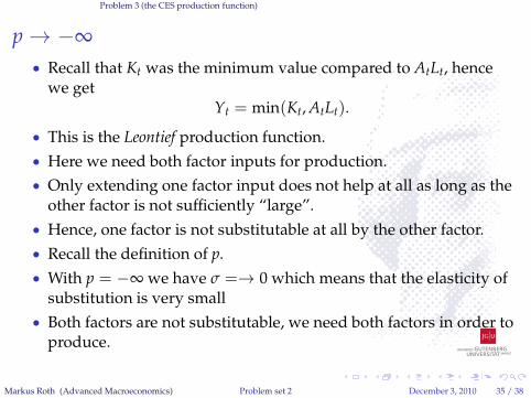
p → −∞

• Recall that Kt was the minimum value compared to AtLt, hencewe get

Yt = min(Kt,AtLt).

• This is the Leontief production function.

• Here we need both factor inputs for production.

• Only extending one factor input does not help at all as long as theother factor is not sufficiently “large”.

• Hence, one factor is not substitutable at all by the other factor.


• With p = −∞ we have σ =→ 0 which means that the elasticity ofsubstitution is very small

• Both factors are not substitutable, we need both factors in order toproduce.



0

1

2

3

4

5

0

1

2

3

4

50

1

2

3

4

5

F(K,L)

K

L

F(K,L)

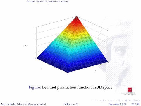
Figure: Leontief production function in 3D space



0

1

2

3

4

5

0 1 2 3 4 5

L

K

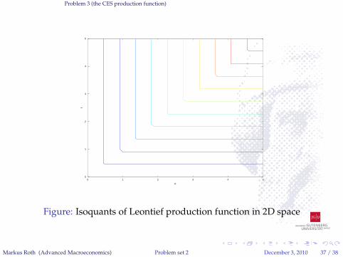
Figure: Isoquants of Leontief production function in 2D space


References

References

La Grandville, O. D. (2009).Economic Growth: A Unified Approach.Cambridge University Press.

Romer, D. (2005).Advanced macroeconomics.Mcgraw-Hill Higher Education, 3. ed. edition.

Wickens, M. (2008).Macroeconomic Theory: A Dynamic General Equilibrium Approach.Princeton University Press.


Documents

Problem set 2 - Welcome to the Chair in Macroeconomics! 1 Problem 1 (differential equations) 2 Problem 2 (the Solow growth model in discrete time) 3 Problem 3 (the CES production function)